Report # MATC-MST: 120 Final Report - Mid-America...

®

The contents of this report reflect the views of the authors, who are responsible for the facts and the accuracy of the information presented herein. This document is disseminated under the sponsorship of the Department of Transportation

University Transportation Centers Program, in the interest of information exchange. The U.S. Government assumes no liability for the contents or use thereof.

A Framework for the Nationwide Multimode Transportation Demand Analysis

Report # MATC-MST: 120 Final Report

Hojong Baik, Ph.D.Assistant ProfessorDepartment of Civil, Architectural and Environmental EngineeringMissouri University of Science and Technology

Yuepeng CuiTao Li

2011

A Cooperative Research Project sponsored by the U.S. Department of Transportation Research and Innovative Technology Administration

A Framework for the Nationwide Multimode Transportation Demand Analysis

Hojong Baik

Assistant Professor

Civil, Arch & Environ Engineering Department

Missouri University of Science and Technology

Yuepeng Cui

Graduate Student



Tao Li

Graduate Student



A Report on Research Sponsored By

Mid-America Transportation Center

University of Nebraska-Lincoln

September, 2010

ii

Technical Report Documentation Page

1. Report No.

25-1121-0001-120

2. Government Accession No.

3. Recipient's Catalog No.

4. Title and Subtitle

A Framework for the Nationwide Multimode Transportation Demand

Analysis

5. Report Date

September, 2010

6. Performing Organization Code

7. Author(s) Dr. Hojong Baik, Yuepeng Cui, and Tao Li

8. Performing Organization Report No.

25-1121-0001-120

9. Performing Organization Name and Address

Mid-America Transportation Center

2200 Vine St.

PO Box 830851

Lincoln, NE 68583-0851

10. Work Unit No. (TRAIS)

11. Contract or Grant No.

12. Sponsoring Agency Name and Address

USDOT RITA

1200 New Jersey Avenue, SE

Washington, DC 20590

13. Type of Report and Period Covered

Draft Report,

14. Sponsoring Agency Code

MATC TRB RiP No. 17128

15. Supplementary Notes

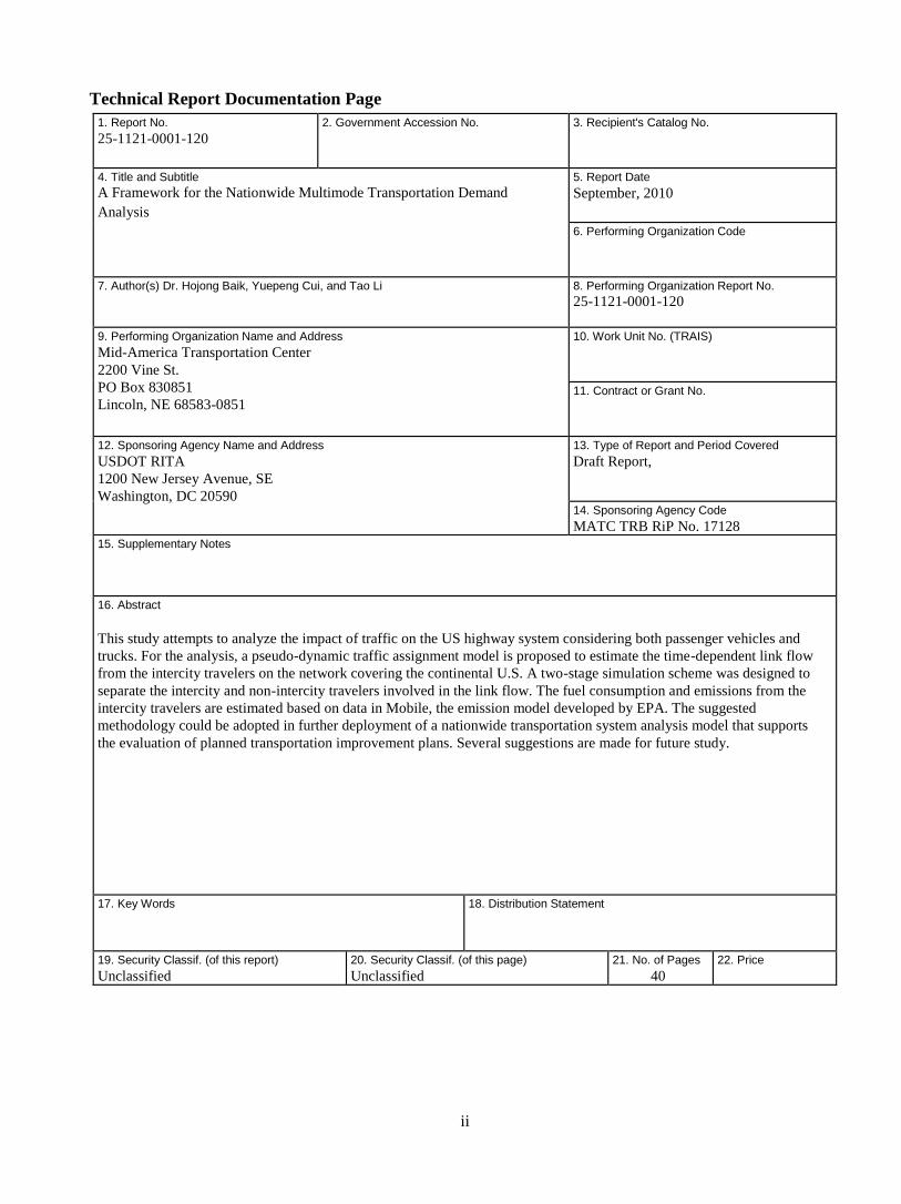
16. Abstract

This study attempts to analyze the impact of traffic on the US highway system considering both passenger vehicles and

trucks. For the analysis, a pseudo-dynamic traffic assignment model is proposed to estimate the time-dependent link flow

from the intercity travelers on the network covering the continental U.S. A two-stage simulation scheme was designed to

separate the intercity and non-intercity travelers involved in the link flow. The fuel consumption and emissions from the

intercity travelers are estimated based on data in Mobile, the emission model developed by EPA. The suggested

methodology could be adopted in further deployment of a nationwide transportation system analysis model that supports

the evaluation of planned transportation improvement plans. Several suggestions are made for future study.

17. Key Words

18. Distribution Statement

19. Security Classif. (of this report)

Unclassified

20. Security Classif. (of this page)

Unclassified

21. No. of Pages

40

22. Price

iii

Table of Contents

CHAPTER 1 INTRODUCTION ................................................................................................... 1

CHAPTER 2 METHODOLOGY ................................................................................................. 5

2.1 Computation Issues and Simulation Assumptions ............................................ 5

2.2 Simulation Model .............................................................................................. 6

2.3 Shortest Path Algorithm .................................................................................... 8

CHAPTER 3 INPUT DATA ....................................................................................................... 9

3.1 Network.............................................................................................................. 9

3.2 Link Performance Function ............................................................................. 15

3.3 Time-Dependent Intercity Traveler Origin-Destination Demand ................... 18

3.4 Time-Dependent Link Flow ............................................................................ 19

3.5 Fuel Consumption and Emission Rates ........................................................... 21

CHAPTER 4 SIMULATION AND RESULTS .............................................................................. 23

CHAPTER 5 CONCLUSIONS AND RECOMMENDATIONS FOR FUTURE RESEARCH .................. 38

REFERENCES ....................................................................................................................... 39

iv

List of Figures

Figure 2.1 Example on How to Calculate the Vehicle Distribution in the Queue ............... 6

Figure 2.2 Flow Chart of the Pseudo-Dynamic Traffic Assignment ................................... 7

Figure 3.1 The US Highway Network and County Centroid ............................................ 14

Figure 3.2 Percentage of Departure During a Typical Day ............................................... 19

Figure 3.3 Daily Distribution of Vehicles by Vehicle Type .............................................. 20

Figure 3.4 Relationship between Emission Rate and Speed for Freeway and Arterial ..... 22

Figure 4.1 Flow Chart of the Simulation Procedure .......................................................... 24

Figure 4.2 Locations of the Selected Roads ...................................................................... 25

Figure 4.3 Direction A of Road 144891 (Rural Freeway) ................................................. 27

Figure 4.4 Direction B of Road 144891 (Rural Freeway) ................................................. 28

Figure 4.5 Direction A of Road 12494 (Urban Freeway) .................................................. 28

Figure 4.6 Direction B of Road 12494 (Urban Freeway) .................................................. 29

Figure 4.7 Direction A of Road 7807 (Rural Arterial) ...................................................... 30

Figure 4.8 Direction B of Road 7807 (Rural Arterial) ...................................................... 30

Figure 4.9 Direction A of Road 12417 (Urban Arterial) ................................................... 31

Figure 4.10 Direction B of Road 12417 (Urban Arterial) ................................................. 31

Figure 4.11 Direction A of Road 181719 (Rural Local) ................................................... 32

Figure 4.12 Direction B of Road 181719 (Rural Local) .................................................... 32

Figure 4.13 Direction A of Road 24194 (Urban Local) .................................................... 33

Figure 4.14 Direction B of Road 24194 (Urban Local)…………………………………..33

Figure 4.15 Total Volume of Intercity Travelers and All Travelers from

0:00 AM to 6:00 AM ............................................................................................ 34


6:00 AM to 12:00 PM ............................................................................................ 35


12:00 PM to 6:00 PM ........................................................................................... 35

v


6:00 PM to 0:00 AM ............................................................................................. 36

Figure 4.19 Total CO2 Emissions from Intercity Travelers Every 6 Hours ..................... 37

vi

List of Tables

Table 3.1 Description of RUCODE ............................................................................................. .. 10

Table 3.2 Description of Functional Class .................................................................................. .. 10

Table 3.3 Directional Roadways by Functional Class and State ................................................. .. 11

Table 3.4 Selection of J Value ....................................................................................................... 17

Table 3.5 Assignment of Speed Limit and Signals per mile ......................................................... 18

Table 3.6 Passenger Car Equivalence (PCE) Factors by Vehicle Type ........................................ 20

Table 3.7 Roadway Types in Mobile-6 and FAF2 ....................................................................... . 22

Table 4.1 Information on the Selected Roads ................................................................................ 26

vii

Acknowledgements

This report is based on research sponsored by the Mid-America Transportation Center (MATC),

Missouri DOT (MoDOT), and the Federal Highway Administration (FHWA) of the US Department of

Transportation (USDOT). The research was performed at Missouri University of Science and Technology

and the contents of this paper reflect the views of the authors, who are responsible for the facts and the

accuracy of the data presented herein. The contents do not necessarily reflect the official views or policies

of MATC, MoDOT or FHWA. The authors gratefully acknowledge the thoughts and comments provided

by Jeff Viken and Samuel Dollyhigh, at NASA Langley Research center, and Dr. Antonio Trani and

Nicolas Hinze at Virginia Tech during the development of this paper.

viii

Abstract

This study attempts to analyze the impact of traffic on the US highway system considering both

passenger vehicles and trucks. For the analysis, a pseudo-dynamic traffic assignment model is proposed

to estimate the time-dependent link flow from the intercity travelers on the network covering the

continental U.S. A two-stage simulation scheme was designed to separate the intercity and non-intercity

travelers involved in the link flow. The fuel consumption and emissions from the intercity travelers are

estimated based on data in Mobile, the emission model developed by EPA. The suggested methodology

could be adopted in further deployment of a nationwide transportation system analysis model that

supports the evaluation of planned transportation improvement plans. Several suggestions are made for

future study.

1

Chapter 1 Introduction

The number of intercity travelers has been increasing during recent years and this poses a serious

challenge for the current nationwide highway transportation system. In order for transportation planners

and engineers to create efficient modes of transportation, an accurate prediction of the impact of the

intercity travel demand is essential in evaluating or expanding the current transportation system network.

When considering management strategies, the intercity transportation providers, such as Amtrak and

airliners, are particularly interested in long distance traveler demand in association with the travel cost

and travel time experienced by the travelers. For the environmentalist, the amount of pollution generated

by automobiles is of great concern. Cars typically consume more fuel and thus create more emissions per

capita when compared with other long distance public transportation modes, such as trains and planes.

Moreover, the negative effects of those travelers on the transportation system and environment provide

significant incentives for the government to invest funding sources in the infrastructure system or other

alternatives. One of the most important estimates measuring those effects is the traffic pattern of intercity

travelers, for example, how those travelers will be distributed throughout the network.

The primary tool for projecting these estimates of the traffic pattern of intercity travelers has long

been the Static Traffic Assignment (STA). During recent decades, research efforts have focused on

solving the STA problem. According to the assumptions on travelers’ route choice behavior, the solution

methods can be classified into the following four types. The first type is the All or Nothing (AON) traffic

assignment, which assumes that every traveler has perfect information about link travel impedance.

Therefore, the traveler chooses the route with the least travel impedance without considering the effect of

other travelers’ choices. As a result, all origin-destination (OD) demand will use the route with the least

travel impedance connecting the OD pair and no travelers will use any the other connecting routes. The

second type is the User Equilibrium (1) assignment, which assumes that travelers have perfect network

information and consider other travelers when making choices. A User Equilibrium (UE) state is reached

when no traveler can reduce his travel impedance by unilaterally changing his route. In addition, for all

2

the routes connecting the same OD pair, those having non-zero traveler flow will have the same travel

impedance and this impedance is the smallest for this OD pair. The third type is the System Optimal (SO)

traffic assignment, which assumes that travelers choose their routes in such a way that the total travel

time in the network is minimized. This situation cannot exist in reality because under the SO state,

travelers can reduce their travel impedance by unilaterally changing their routes. Usually, it serves as a

yardstick by which the performance of different flow patterns can be measured. The last type is the

Stochastic User Equilibrium (SUE) traffic assignment, which considers the travelers’ preference and

perception errors with a certain probability density function. In SUE assignment, travelers choose the

routes with minimum perceived travel impedance. A SUE is reached when no travelers can reduce his

perceived travel impedance by unilaterally changing his route.

The four types of STA do provide important benefits in transportation planning, but there are

significant drawbacks. In STA, the dynamic features of traffic demand and network conditions are

ignored. As is easily observed, traffic flows are not necessarily uniformly distributed, but fluctuate over

time, especially during the rush hour. It is logical that congestion and delays may occur at different

locations at different time. For example, according to traffic flow data, drivers may experience more

delays from 7:00 AM to 8:30 AM on suburban roads, and from 7:00 AM to 9:30 AM on highways than

any other time period. This shortcoming of STA makes it an inadequate tool to model intercity traffic

assignment. STA may significantly underestimate the congestion effects caused by temporary intercity

demand exceeding the capacity as STA relies on the uniformly distributed average intercity demand,

which may turn out to be far less than the capacity. Furthermore, STA cannot capture the speed variance

of intercity drivers resulting from the dynamics of local traffic. Intercity travelers have to share roads with

local drivers, thus the local dynamic traffic conditions will have a significant influence on the speed of

intercity travelers. For instance, the intercity travelers may be slowed down by the local stop-and-go type

of traffic during the peak hours. Speed variance is a very crucial factor that influences emissions and fuel

consumption. Unfortunately, this effect cannot be appropriately captured by the STA methods. In fact,

3

emissions and fuel consumption is potentially underestimated by STAP methods. The third issue is that

some intercity travelers choose their departure time or even part of their routes to avoid expected

congestions at certain time periods. In STA methods, the drivers’ dynamic choice behaviors cannot be

accounted for since no such information can be provided on time-variant traffic condition.

Due to the shortcomings of STA, it was necessary to develop other approaches for transportation

planning and management. Dynamic Traffic Assignment (DTA) provides an effective way to estimate the

time-dependent traffic flow and speed variance in the network. Besides the time-dependent OD demand,

one of the major differences between STA and DTA concerns link travel impedance. In STA, it is

assumed the instantaneous link travel impedance measured at the moment when the travelers choose their

routes is the travel impedance they will experience in the network. It is also assumed that travelers will

contribute to the flows of all the links that are on the selected routes. In DTA, as travelers move along

their routes, new travelers will keep entering the network and share the same roadways. Travelers’

experienced travel impedance may be different from the instantaneous travel impedance estimated when

entering the network because those who enter afterwards may have more significant impact on link travel

impedance. Moreover, at each moment, each traveler can contribute to the flow of only one link on his

route. If all of the time-dependent OD information is available over the entire period of study, then the

concepts for the STA can be generalized to the time-dependent case (2). The route travel impedance is

computed based on the time-dependent link impedance instead of the instantaneous link impedance. This

general overview served to provide some insight to the advantages of DTA models before examining

DTA in more detail.

DTA models are typically classified into two categories: mathematical and simulation based.

Peeta and Ziliaskopoulos (3) and Peeta (4) provide an excellent review of the two approaches.

Mathematical approaches can be further divided into three sub-categories: mathematical programming

models as proposed by Janson (6), Smith (7), and Ziliaskopoulos (8); optimal control theory based

formulations designed in Friesz, et al (9); and variational inequality methods introduced in Boyce, et al

4

(10), Lee (11), Ran, et al (12), and Ran et al (13). Most mathematical formulations are a generalization of

their equivalent static formulations and suffer from two main disadvantages. First, they may not be able

to adequately capture the realities due to over simplifications of networks’ topology and driver behaviors.

Second, they are generally difficult to solve mathematically and tend to be intractable for large size

networks.

Simulation based approaches overcome these disadvantages and have been incorporated in

solution algorithms to be used directly for a solution. For example, DYNASMART is incorporated as a

simulator in the solution algorithms proposed by Peeta and Mahmassani (2); Mahmassani, et al (14);

Peeta and Mahmassani (15); and Ziliaskopoulos, et al (16). DYNAMIT is also utilized as part of the DTA

system intended for generating real-time prediction-based guidance information by Ben-Akiva, et al (17).

Although simulation models can’t provide the analytical insight and guarantee the uniqueness and

convergence of the solution, they have been considered an efficient way to reduce the mathematical

complexity, as well as computational time. In this study, a simulation method is developed and adopted

for the DTA. The goal of this study is to propose a pseudo-dynamic traffic assignment (PDTA), which

can give a fair estimation of the time-dependent traffic flow pattern, emissions, and fuel consumption

resulting from the intercity demand for the continental U.S. transportation network.

The report is organized as follows: the methodology is given in chapter 2, input data is presented in

chapter 3, simulation results and analysis are shown in chapter 4, and the conclusions and recommended

future work are discussed in chapter 5.

5

Chapter 2 Methodology

2.1 Computation Issues and Simulation Assumptions

In order to further understand the concerns we wish to address, we present the computational

difficulties involved in the PDTA simulation model. Firstly, inter-city traffic assignment at the national

level involves a large-scale network with great variation in traffic conditions. In the simulation model,

vehicle interactions at the microscopic level, such as first in, first out (FIFO) and delay holding, have to

be considered. For a small or even medium network, it is possible to incorporate the microscopic vehicle

interactions but it is impractical for the network scale of our study. Secondly, travelers may stay in the

network for a relatively long period before reaching destinations which would require excessive

computational efforts and memory to trace. Thirdly, travelers with different preferences and trip purposes

may react differently given the same traffic situation. As a result, a large amount of computation time has

to be spent on deciding their shortest routes. To simplify the computational complexity, the following

assumptions are made: 1) Travelers are assumed to be homogeneous in terms of information availability,

the type of information, and their reaction to the information; 2) Travelers are assumed to have no

information about the time-dependent OD demand. Thus, they have no information about the routes

travel impedance from the time-dependent link impedance. However, they do have some static link

information, such as speed limit and local traffic conditions estimated when they depart. They will choose

the shortest routes based on this instantaneous traffic condition; 3) The route travel impedance of

travelers entering the network is assumed not to be affected by those who enter the network afterwards.

This means that travelers choose their routes based on the travel impedance estimated at the moment they

enter the network. Furthermore, the route travel impedance they will experience is assumed to be the

same as the impedance at the moment when they made the decision; 4) The microscopic-level vehicle

interactions are not considered. Instead, the macroscopic relationship between speed and flow is applied

to estimate the delays on each link.

6

2.2 Simulation Model

Our simulation is macro-level and based on the supposition that at each time interval, an OD

demand is generated and travelers choose their shortest routes based on the current local traffic flow. All

of the travelers of an OD pair departing at time interval k are assumed to stay together in a queue on their

route (note that based on the aforementioned assumptions 1 and 2, they will stay on the same route with

the least instantaneous travel impedance estimated when entering the network). The queue will never

break but it can be expanded or squeezed based on the traffic conditions. At each time interval, only the

position of the first and last vehicle in the queue is updated and the length of queue is computed as the

distance between the two vehicles. Such scheme has been successively applied to estimate the assignment

matrix for Kalman Filter (18). The vehicle distribution among the links that form the queue depends on

the links’ travel time. The queue contributes to the flow of the links it covers at each time interval. Figure

2.1 illustrates the calculation of vehicle distribution; where N is the number of vehicles in the queue, T is

the travel time from the tail to the head of the queue, T1 represents the time needed for the tail to reach

node B, T2 is the travel time from node B to C, T3 means the travel time needed to travel from node C to

the head. Figure 2.2 presents the flow chart of the pseudo-dynamic traffic assignment scheme. The

simulation procedure in its entirety can be found in chapter 4.

Figure 2.1 Example on How to Calculate the Vehicle Distribution in the Queue

7

Figure 2.2 Flow Chart of the Pseudo-Dynamic Traffic Assignment

8

2.3 Shortest Path Algorithm

The algorithm utilized in our study is known as the label−correcting method. It finds the shortest

path from a given origin to all other nodes in the network. A detail description of the algorithm is

presented in Sheffi’s research (19). The shortest path algorithm is implemented using parallel computing

toolbox available in Matlab.

9

Chapter 3 Input Data

3.1 Network

The Freight Analysis Framework-2 (FAF2) network originally prepared for analyzing freight

movement by truck encompasses the highway system in the continental US and Alaska (Alaska not

included in this study). The network data contains information about the length, direction, capacity,

Annual Average Daily Traffic (AADT), and AADTT (Annual Average Daily Truck Traffic) on each link

of roadways. While FAF2 provides AADT and AADTT in both directions for bi-directional roadways,

the capacity is given for one direction on multilane facilities and for both directions on 2-or 3-lane

facilities. Note that FAF2 data only contains information about whether the road is bi-directional or not,

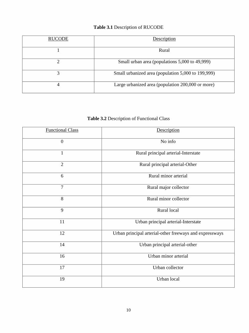
no further details are given. Each roadway link is assigned to a RUCODE) and a Functional Class

(FClass) denoting its location and the functional type, respectively. The corresponding descriptions are

given in tables 3.1 and 3.2. Table 3.3 summarizes the distribution of directional roadways by FClass and

state.

The number of lanes is inevitable information in characterizing the link performance function,

namely speed-volume (or speed-delay) relationship. However, it should be pointed out that the number of

lanes on each roadway is not provided in FAF2. In order to overcome this practical impediment, the

directional capacity is estimated by assuming the capacity of roads with functional class 1, 2, 11, and 12

are given in one direction, and the others in both directions. Some pre-processing effort is also applied to

the original network, for instance fixing the link connectivity and missing data. So as to represent an

aggregate of trip origins and destinations, a total of 3,625 traffic nodes (3,076 county centroids plus 549

airports) were added to the original network, as well as 3,625 bi-direction connectors that connect the

traffic nodes to the highway network. It is assumed that the connectors have an infinite capacity with

zeros travel impedance. The highway network and traffic nodes are illustrated in figure 3.1.

10

Table 3.1 Description of RUCODE

RUCODE Description

1 Rural

2 Small urban area (populations 5,000 to 49,999)

3 Small urbanized area (population 5,000 to 199,999)

4 Large urbanized area (population 200,000 or more)

Table 3.2 Description of Functional Class

Functional Class Description

0 No info

1 Rural principal arterial-Interstate

2 Rural principal arterial-Other

6 Rural minor arterial

7 Rural major collector

8 Rural minor collector

9 Rural local

11 Urban principal arterial-Interstate

12 Urban principal arterial-other freeways and expressways

14 Urban principal arterial-other

16 Urban minor arterial

17 Urban collector

19 Urban local

Table 3.3 Directional Roadways by Functional Class and State

FClass/

State AL AK AZ AR CA CO CT DE DC FL GA HI ID IL IN IA KS

1 122 82 138 76 274 142 18 0 0 220 244 0 74 324 162 120 108

2 446 54 142 480 717 346 44 90 0 908 1022 70 218 710 398 826 662

6 792 52 160 604 1274 468 194 78 0 788 1998 90 158 1125 458 752 756

7 10 4 10 4 16 4 0 0 0 2 20 0 0 0 6 6 0

8 0 0 0 0 0 2 0 0 0 0 0 0 0 0 0 0 0

9 0 0 0 2 0 0 0 0 0 0 2 0 0 0 0 2 0

11 206 54 158 188 1535 206 282 46 38 386 368 68 75 638 280 134 200

12 22 0 166 90 1876 224 326 20 50 355 124 30 0 74 122 0 142

14 801 80 1222 774 10571 1162 930 286 352 2688 2284 230 498 3016 1515 794 885

16 24 20 28 8 209 42 8 4 4 254 63 2 0 181 0 44 2

17 0 2 8 0 42 12 2 0 0 20 18 2 12 110 0 4 4

19 0 0 0 0 0 0 0 0 0 12 4 0 0 41 0 10 0

Noninfo 460 390 315 386 436 249 502 78 56 748 1361 278 218 352 290 314 302

Missing 0 0 0 0 0 0 0 0 0 0 0 0 0 0 0 0 0

Total 2883 738 2347 2612 16950 2857 2306 602 500 6381 7508 770 1253 6571 3231 3006 3061

11

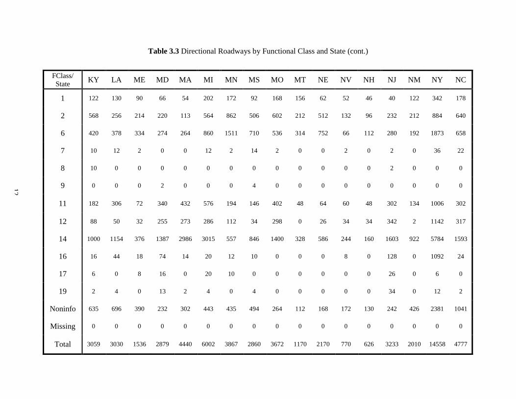
Table 3.3 Directional Roadways by Functional Class and State (cont.)

FClass/

State KY LA ME MD MA MI MN MS MO MT NE NV NH NJ NM NY NC

1 122 130 90 66 54 202 172 92 168 156 62 52 46 40 122 342 178

2 568 256 214 220 113 564 862 506 602 212 512 132 96 232 212 884 640

6 420 378 334 274 264 860 1511 710 536 314 752 66 112 280 192 1873 658

7 10 12 2 0 0 12 2 14 2 0 0 2 0 2 0 36 22

8 10 0 0 0 0 0 0 0 0 0 0 0 0 2 0 0 0

9 0 0 0 2 0 0 0 4 0 0 0 0 0 0 0 0 0

11 182 306 72 340 432 576 194 146 402 48 64 60 48 302 134 1006 302

12 88 50 32 255 273 286 112 34 298 0 26 34 34 342 2 1142 317

14 1000 1154 376 1387 2986 3015 557 846 1400 328 586 244 160 1603 922 5784 1593

16 16 44 18 74 14 20 12 10 0 0 0 8 0 128 0 1092 24

17 6 0 8 16 0 20 10 0 0 0 0 0 0 26 0 6 0

19 2 4 0 13 2 4 0 4 0 0 0 0 0 34 0 12 2

Noninfo 635 696 390 232 302 443 435 494 264 112 168 172 130 242 426 2381 1041

Missing 0 0 0 0 0 0 0 0 0 0 0 0 0 0 0 0 0

Total 3059 3030 1536 2879 4440 6002 3867 2860 3672 1170 2170 770 626 3233 2010 14558 4777

12

Table 3.3 Directional Roadways by Functional Class and State (cont.)

FClass/

State ND OH OK OR PA RI SC SD TN TX UT VT VA WA WV WI WY Missing

1 88 200 142 120 336 8 206 122 132 408 116 76 208 118 96 176 116 0

2 554 746 380 356 958 42 438 428 428 1132 122 94 446 415 284 1002 234 2

6 332 674 458 390 1694 42 956 514 660 1440 218 180 852 352 362 1136 146 2

7 0 20 4 4 4 0 0 0 2 30 0 0 2 4 0 0 0 0

8 0 0 0 0 0 0 0 0 0 2 0 0 0 0 0 0 0 0

9 0 0 0 8 0 0 0 0 0 0 0 0 0 0 0 0 0 0

11 48 801 234 196 490 86 136 54 328 1200 148 34 378 364 106 196 72 0

12 0 556 158 80 524 92 60 0 112 1195 10 34 258 521 36 253 2 0

14 192 2805 910 1198 3768 602 708 298 1266 6162 257 126 1212 2554 388 1849 190 0

16 0 57 94 60 38 2 0 0 34 165 2 0 42 63 0 12 0 0

17 0 26 0 30 43 2 0 0 10 82 0 0 2 10 0 4 0 0

19 0 48 0 24 0 0 0 0 6 0 0 0 0 0 0 0 0 0

Non-

info 178 571 478 302 629 44 270 98 330 1742 190 168 616 855 234 520 238 2

Missing 0 0 0 0 0 0 0 0 0 0 0 0 0 0 0 0 0 20

Total 1392 6504 2858 2768 8484 920 2774 1514 3298 13560 1063 712 4016 5256 1506 5148 998 26

13

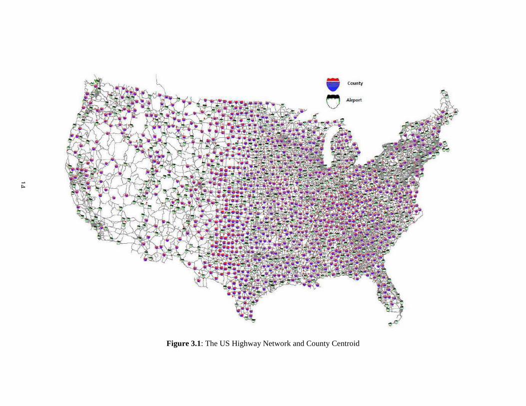
Figure 3.1: The US Highway Network and County Centroid

14

15

3.2 Link Performance Function

Link performance function plays a key role in the traffic assignment. It provides a

measurement of the link travel impedance, for instance travel time or travel time reliability.

Among various types of functions, the Bureau of Public Roads (BPR) function is widely adopted

by the planners. The function is given as by:

TT = FFT × (1 + α (V /C)β) (3.1)

where, TT is the link travel time, FFT is the link free flow travel time, α > 0 and β > 0 are

parameters to be calibrated (typically α = 0.15, β = 4.0), V is the link volume, and C is the

link capacity.

Note that BPR function is convex and derivable in terms of V, which ensures certain

desirable properties, such as uniqueness of any optimization problem using the function,

resulting in computational simplicity. However, FAF2 data set contains no information about the

parameters α and β for each link.

Another way for estimating the link travel time is to use a heuristic equation derived from

the observational data. The following equation is the one that the Highway Capacity Manual

(HCM) (21) offers based on the traffic data collected for years:

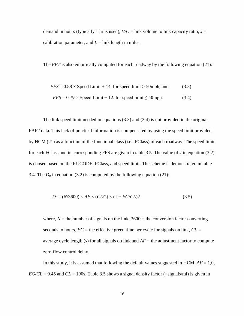
𝑇𝑇=𝐹𝐹𝑇+𝐷0+ 0.25×𝑇×[ 𝑉𝐶−1 + 𝑉𝐶−1 2+16×𝐽×𝑉/𝐶×𝐿2𝑇2 (3.2)

where, TT = the travel time in hours, FFT = the free flow travel time in hours, D0 = zero

flow control delay at signalized intersections in hours, T = the expected duration of

16

demand in hours (typically 1 hr is used), V/C = link volume to link capacity ratio, J =

calibration parameter, and L = link length in miles.

The FFT is also empirically computed for each roadway by the following equation (21):

FFS = 0.88 × Speed Limit + 14, for speed limit > 50mph, and (3.3)

FFS = 0.79 × Speed Limit + 12, for speed limit ≤ 50mph. (3.4)

The link speed limit needed in equations (3.3) and (3.4) is not provided in the original

FAF2 data. This lack of practical information is compensated by using the speed limit provided

by HCM (21) as a function of the functional class (i.e., FClass) of each roadway. The speed limit

for each FClass and its corresponding FFS are given in table 3.5. The value of J in equation (3.2)

is chosen based on the RUCODE, FClass, and speed limit. The scheme is demonstrated in table

3.4. The D0 in equation (3.2) is computed by the following equation (21):

D0 = (N/3600) × AF × (CL/2) × (1 − EG/CL)2 (3.5)

where, N = the number of signals on the link, 3600 = the conversion factor converting

seconds to hours, EG = the effective green time per cycle for signals on link, CL =

average cycle length (s) for all signals on link and AF = the adjustment factor to compute

zero-flow control delay.

In this study, it is assumed that following the default values suggested in HCM, AF = 1,0,

EG/CL = 0.45 and CL = 100s. Table 3.5 shows a signal density factor (=signals/mi) is given in

17

HCM as a function of FClass. Then, the N of each road in equation (3.5) is calculated by

multiplying its signal density by road length.

Table 3.4 Selection of J Value

RUCODE Type Functional Classification Free Flow Speed (mph) J

1 -- 70.1-85.0 2.69E-05

65.1-70.0 2.10-O5

60.1-65.0 1.48E-05

55.1-60.0 8.65E-06

>55.0 3.31E-06

2 -- 55.1-80.0 2.30E-06

50.1-55.0 2.03E-06

45.1-50.0 1.63E-06

>45.0 2.52E-06

3 -- 63.1-80.0 6.91E-05

56.1-63.0 0.000114

50.1-56.0 0.000202

44.1-50.0 0.000400

>44.0 0.000929

4 14 -- 0.000468

16 0.000502

17 0.004550

19 0.013700

18

Table 3.5 Assignment of Speed Limit and Signals per mile

Functional

Class

Assigned

Speed Limit

(mph)

Free Flow Speed

(mphr)

Signals

per Mile

0 55 62.4 0.6

1 70 75.6 0.0

2 65 71.2 0.2

6 55 62.4 0.6

7 55 62.4 0.6

8 45 47.6 0.6

9 35 39.7 1.9

11 65 71.2 0.0

12 65 71.2 0.2

14 55 62.4 0.6

16 45 47.5 0.6

17 35 39.7 1.9

19 30 35.7 3.1

3.3 Time-Dependent Intercity Traveler Origin-Destination Demand

Defining intercity trips as those that travel longer than 100 miles of one-way distance, an

existing travel demand model named Transportation Systems Analysis Mode (TSAM) estimates

the static intercity travel demand by trip purpose (i.e., business and non-business trips) at the

county level. Its development was based on the concept of the traditional four-step transportation

demand modeling process and TSAM essentially involves a series of sub-models that are

calibrated using travel survey data combined with socio-economic and demographic data [22].

By using average party sizes for each trip purpose collected from the survey data, the traveler

OD tables are converted to the passenger-car OD tables. The resulting static passenger-car OD

tables are then converted to the time-dependent passenger-car demand using the percentage of

departures for every 30-minute interval estimated from Jin and Horowitx (20). Figure 3.2 shows

the distribution of the departures in every 30 minute interval.

19

Figure 3.2 Percentage of Departure During a Typical Day

3.4 Time-Dependent Link Flow

The time-dependent link flow is estimated from the AADT and AADTT in FAF2 data.

The hourly distribution of passenger cars and trucks during one typical day is estimated using the

traffic sensor data collected by Missouri Department of Transportation (MoDOT) using the

Remote Traffic Microwave Sensor (RTMS) system installed on roadways around the St. Louis

area. The sensor data contains complete one-year traffic counts of vehicles summarized in hourly

traffic volume. In the data, vehicles are classified into four classes: class 1 is passenger-car, and

classes 2-4 are different types of trucks. The distribution of traffic counts by vehicle class during

a typical day is presented in figure 3.3. The AADTT on each link is split into different types of

trucks for vehicle classes 2, 3, and 4.The number of trucks is then converted to equivalent

20

passenger-cars using Passenger-Car Equivalence (PCE) since V/C in eq. (3.2) is given in

passenger-car. The PCE conversion factors for each vehicle class are given in table 3.6.

Table 3.6 Passenger Car Equivalence (PCE) Factors by Vehicle Type

Class 1 Class 2 Class 3 Class 4

PCE 1.0 1.2 1.5 2.5

Figure 3.3 Daily Distribution of Vehicles by Vehicle Type

It should be noted that the time-dependent traveler passenger-car (vehicle class 1) flow

on roadways is composed of two different types of travelers: time-dependent inter-city and local

or intra-city travelers. Note that the number of passenger cars by local travelers will serve as

21

input preloaded on the network before assigning the intercity demand. However, no information

of the local travelers is available in FAF2. To separate the time-dependent local traveler flow

from the total passenger car flows on each link, a two-stage simulation scheme is utilized in our

study. The detailed procedure will be discussed in the following section.

3.5 Fuel Consumption and Emission Rates

The inputs for the fuel consumption and emission are inferred from Mobile-6 developed

by the Environmental Protection Agency (EPA). Mobile-6 is a computer program that estimates

the emission rates (grams/mi) by considering various local factors, such as vehicle mix, speed,

temperature, and so on. For computational simplicity, it is assumed that most passenger cars are

light duty gasoline vehicles (LDGV) whose fuel consumption is, on average, about 23.9 mpg

obtained from Mobile-6. Four kinds of emission are investigated in our study: CO2, THC (Total

hydrocarbon), CO, and NOx. The emission rate of CO2 is a given constant (371.2 gram/mi) in

Mobile-6, whereas the emission rates of the other three components are functions of road type

and average speed. In Mobile-6, three major road types are considered: freeway, arterial, and

local roadway. Each roadway link in FAF2 is classified into one of the three road types defined

in Mobile-6 according to its FClass in FAF2. The matching table used in the classification

procedure is shown in table 3.7. Figure 3.4 shows the relationship between the emission rates and

speed interpolated from Mobile-6 outputs for the freeway and arterial roadways. For the roads

with local type, the following fixed emission rates are applied: 2.196 (gram/mi) for THC, 1.124

(gram/mi) for Nox, and 12.84(gram/mi) for CO.

22

Table 3.7 Roadway Types in Mobile-6 and FAF2

Freeway Arterial Local

FClass in FAF2 1, 2, 11, 12 6, 7, 14, 16 8, 9, 17, 19, and others

Figure 3.4 Relationship between Emission Rate and Speed for Freeway and Arterial

23

Chapter 4 Simulation and Results

In the simulation, the travel time is assumed to be the travel impedance. As mentioned in

chapter 3, a two-stage simulation scheme is used to estimate the time-dependent local traveler

flow, which is described below.

Stage 1: Load the time-dependent link flow estimated from AADT and AADTT as the time-

dependent local traveler flow. Do the pseudo-DTA to get the time-dependent intercity flow.

Compute the time-dependent local traveler flow by subtracting this flow from the time-

dependent flow.

Stage 2:

Step 1. Load the new time-dependent non-intercity flow and do the pseudo-DTA to get the time-

dependent intercity flow.

Step 2. Calculate the new time-dependent non-intercity flow and check the termination

condition, if it is met, then stop; otherwise go back to step 1.

The whole simulation procedure is illustrated in figure 4.1. Six bi-direction roads were

picked for analysis. Table 4.1 presents the detailed information about those roads, and their

locations are given in figure 4.2. Based on Tables 3.2 and 3.7, the first and second roads are a

rural and urban freeway respectively, the third and fourth are a rural and urban arterial

respectively, and the fifth and sixth are local roadways. Since no detail is given about the

directions of bi-direction roads, the two directions of those roads are called directions A and B

arbitrarily.

24

Figure 4.1 Flow Chart of the Simulation Procedure

Figure 4.2 Locations of the Selected Roads

25

26

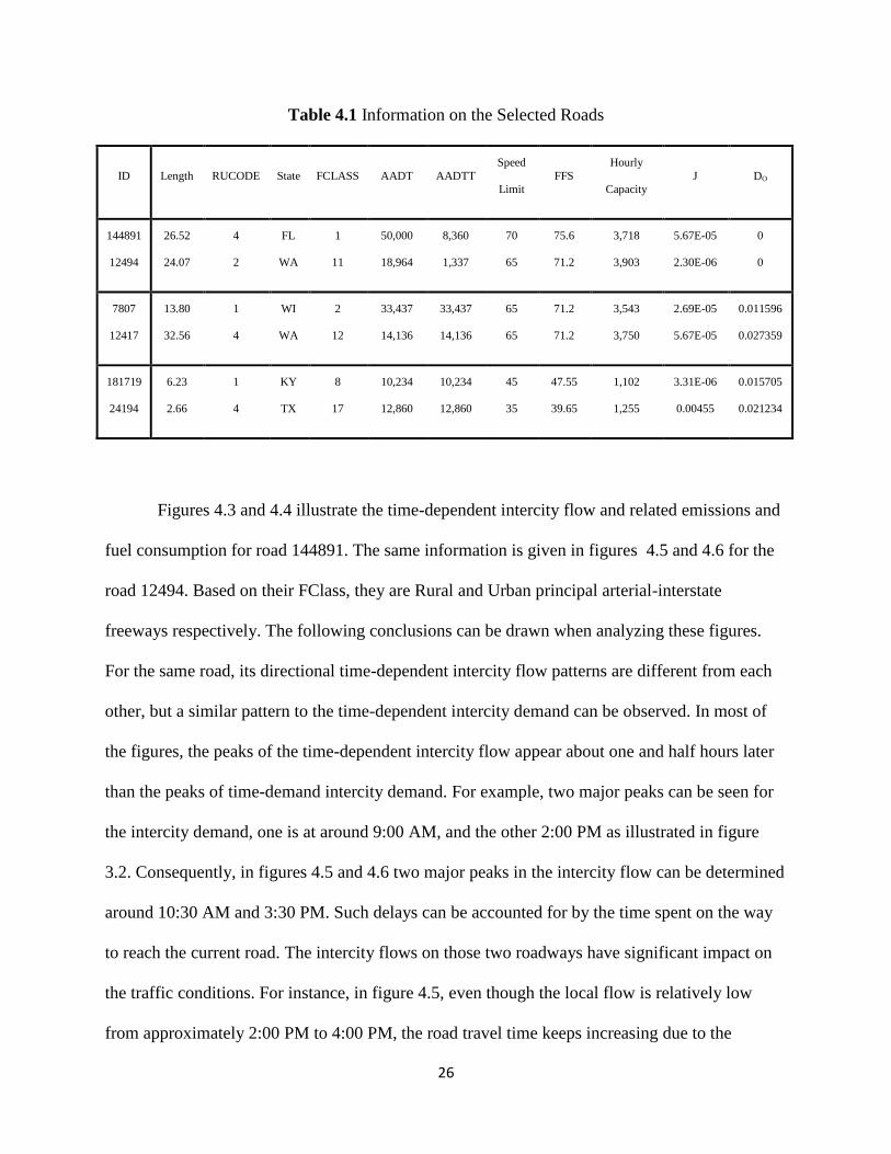
Table 4.1 Information on the Selected Roads

ID Length RUCODE State FCLASS AADT AADTT

Speed

Limit FFS

Hourly

Capacity J DO

144891

12494

26.52

24.07

4

2

FL

WA

1

11

50,000

18,964

8,360

1,337

70

65

75.6

71.2

3,718

3,903

5.67E-05

2.30E-06

0

0

7807

12417

13.80

32.56

1

4

WI

WA

2

12

33,437

14,136

33,437

14,136

65

65

71.2

71.2

3,543

3,750

2.69E-05

5.67E-05

0.011596

0.027359

181719

24194

6.23

2.66

1

4

KY

TX

8

17

10,234

12,860

10,234

12,860

45

35

47.55

39.65

1,102

1,255

3.31E-06

0.00455

0.015705

0.021234

Figures 4.3 and 4.4 illustrate the time-dependent intercity flow and related emissions and

fuel consumption for road 144891. The same information is given in figures 4.5 and 4.6 for the

road 12494. Based on their FClass, they are Rural and Urban principal arterial-interstate

freeways respectively. The following conclusions can be drawn when analyzing these figures.

For the same road, its directional time-dependent intercity flow patterns are different from each

other, but a similar pattern to the time-dependent intercity demand can be observed. In most of

the figures, the peaks of the time-dependent intercity flow appear about one and half hours later

than the peaks of time-demand intercity demand. For example, two major peaks can be seen for

the intercity demand, one is at around 9:00 AM, and the other 2:00 PM as illustrated in figure

3.2. Consequently, in figures 4.5 and 4.6 two major peaks in the intercity flow can be determined

around 10:30 AM and 3:30 PM. Such delays can be accounted for by the time spent on the way

to reach the current road. The intercity flows on those two roadways have significant impact on

the traffic conditions. For instance, in figure 4.5, even though the local flow is relatively low

from approximately 2:00 PM to 4:00 PM, the road travel time keeps increasing due to the

27

significant increase in the intercity flow during this period. A similar situation is demonstrated in

figures 4.3 and 4.6. Since both of the roads are classified as freeways, the emissions of THC,

CO, and NOx are functions of speed only. Note that the speeds on both roads are greater than 60

mph, and as shown in figure 3.4, the emission rates (gram/mi) are almost constants for the three

emissions in this case. Moreover, the emission of CO2 is assumed to be constant (371.2

gram/mi) too. Therefore, the total emission rates (v-gram/h) are functions of VMT rate (v-mi/h).

This also can be observed from the similarity of the dynamic patterns between VMT rates and

emission rates.

Figure 4.3 Direction A of Road 144891 (Rural Freeway)

28

Figure 4.4 Direction B of Road 144891 (Rural Freeway)

Figure 4.5 Direction A of Road 12494 (Urban Freeway)

29

Figure 4.6 Direction B of Road 12494 (Urban Freeway)

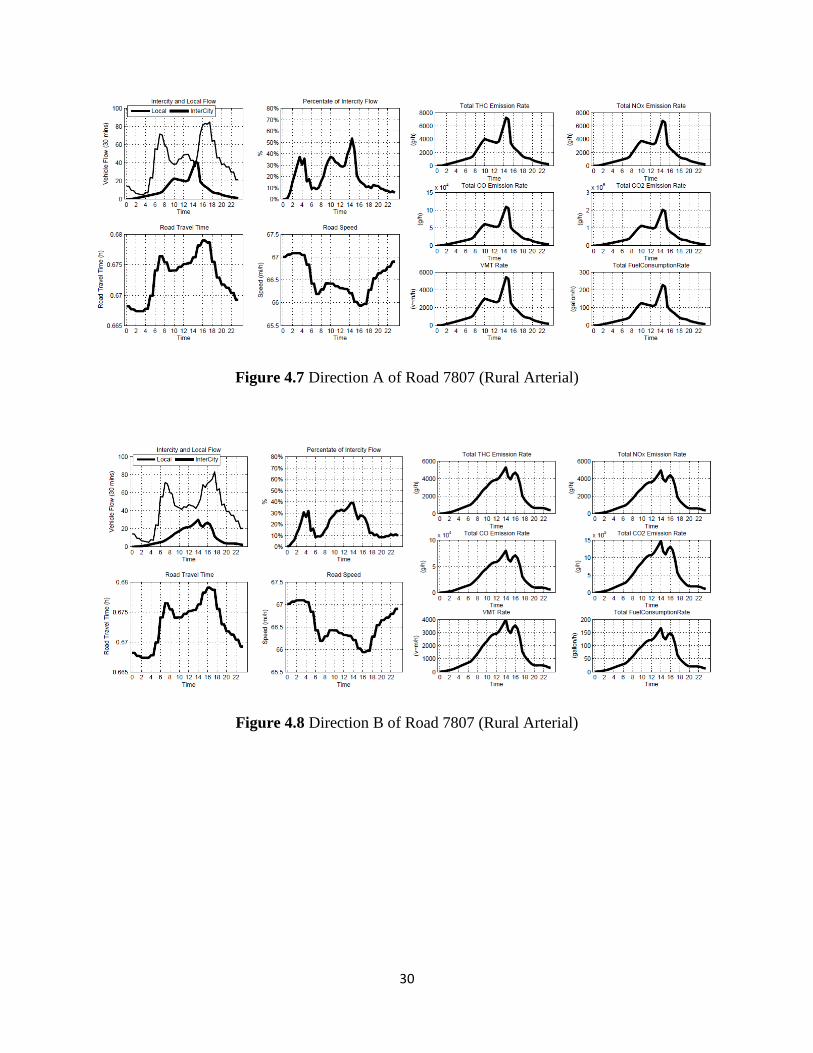
The third (7807) and fourth (12417) roads are classified as rural and urban arterial,

respectively. Their time-dependent road flows and emission rates are illustrated in figures 4.7,

4.8, 4.9, and 4.10,. Two differences can be observed when compared to the two roads (144891

and 12494) previously discussed. First, the occurrences of intercity flow peaks are very close to

those of intercity demand. This is an indication that there may be trip origins around the roads.

Second, there is a smaller percentage of intercity vehicles than found on roads 144891 and

12494, which complies with the reasonable notion that intercity travelers are more willing to take

the freeways which are generally faster than the arterial roads. Similarly, the emissions and fuel

consumptions are dominated by the VMT rate because of the relatively high speed on roads

144891 and 12494.

30

Figure 4.7 Direction A of Road 7807 (Rural Arterial)

Figure 4.8 Direction B of Road 7807 (Rural Arterial)

31

Figure 4.9 Direction A of Road 12417 (Urban Arterial)

Figure 4.10 Direction B of Road 12417 (Urban Arterial)

The last two roads 181719 (urban collector) and 24194 (rural minor collector), are

classified as local in table 3.4. Figures 4.11 and 4.12 present the time-dependent intercity and

local flows and figures 4.13 and 4.14 offer the corresponding emissions and fuel consumption

rates. Relatively small amount of intercity flow can be seen and they have little influence on the

32

traffic condition in those cases. Roads of this kind are not preferred by the intercity travelers

because of their low capacities and low speed limits. The patterns of total emission rates are

similar to that of total VMT rates since the emission rates are constants for the roads of local

type.

Figure 4.11 Direction A of Road 181719 (Rural Local)

Figure 4.12 Direction B of Road 181719 (Rural Local)

33

Figure 4.13 Direction A of Road 24194 (Urban Local)

Figure 4.14 Direction B of Road 24194 (Urban Local)

Figures 4.15, 4.16, 4.17, and 4.18 illustrate the intercity vehicles and total vehicles on the

roads with FClass 1, 2, 11, and 12 every 6 hours. Relatively fewer vehicles can be observed from

0:00 AM to 6:00 AM and 6:00 PM to 0:00 AM on the map for both groups which fulfills

common sense expectations that a relatively small number of travelers will be on the road during

34

those time periods. Meanwhile, a large number of vehicles are on the road from 6:00 AM to

12:00 PM and 12:00 PM to 6:00 PM. Observable differences exist in the intercity vehicle volume

for those two time periods. The volume from 12:00 PM to 6:00 PM is greater than from 6:00 AM

to 12:00 PM because the largest peak in the departure for the intercity travelers happens in the

afternoon. Note that the intercity vehicle volume from 0:00 AM to 6:00 AM is smaller than the

one during 6:00 PM to 0:00 AM even though a higher percentage of departures occur during the

former time period. This is because some of the intercity travelers that departed in the afternoon

or even morning may still be in the network in the evening, which contributes to the intercity

volume during this time period. The total vehicle volume within those two intervals of 6 hours

exhibits a very similar pattern because of the relatively symmetric movement of morning and

afternoon local traffic. However, due to the intercity flows, the total vehicles volume in the

afternoon on certain roads is higher than the volume in the morning.

Figure 4.15 Total Volume of Intercity Travelers and All Travelers from 0:00 AM to 6:00 AM

35

Figure 4.16 Total Volume of Intercity Travelers and All Travelers from 6:00 AM to 12:00 PM

Figure 4.17 Total Volume of Intercity Travelers and All Travelers from 12:00 PM to 6:00 PM

36

Figure 4.18 Total Volume of Intercity Travelers and All Travelers from 6:00 PM to 0:00 AM

37

Figure 4.19 shows the CO2 emissions from the intercity link flows on roads with FClass

1, 2, 11, and 12 every 6 hours. Clearly, the CO2 emissions from 12:00 AM to 6:00 PM is the

highest followed by the CO2 emissions during 6:00 AM to 12:00 AM.

Figure 4.19 Total CO2 Emissions from Intercity Travelers Every 6 Hours

38

Chapter 5 Conclusions and Recommendations for Future Research

In this report, a Pseudo-DTA simulation model is proposed to estimate the time-

dependent intercity flow from the intercity demand across the whole U.S. Also, the fuel

consumption and emission rates are estimated based on the simulation results and data from

EPA’s Mobile-6. Results analysis shows that our simulations model gives a reasonable

estimation of time-dependent intercity flow in an efficient way. However, the following issues

deserve further investigation in the future to improve our method.

First, the US territories span six time zones; therefore, the time-dependent intercity

demand of each OD pair and non-intercity traffic flow on each road should be estimated

according to its local time instead of under the same time horizon.

Secondly, more detailed data on the FAF2 network is expected from the Highway

Performance Monitoring System (HPMS). The road capacity, speed limit, and other related

parameters should be estimated or calculated in a more accurate way.

Thirdly, the traffic counts data used to estimate the time-dependent link flow were

collected from the St. Louis area only, which may not be representative. The use of a more

general traffic counts data set should be considered.

Fourthly, since the time-dependent local flow is known a priori, a dynamic shortest path

algorithm may be considered, which is more reasonable than the one we are currently using.

Lastly, the AADTT in FAF2 includes intercity truck flows, and those trucks are

converted to passenger car unit to be treated as non-intercity flows. Our model may be improved

to better estimate the time-dependent intercity truck and passenger car flow and their related fuel

consumption and emissions.

39

References

1. Wardrop J.G. 1952. Some theoretical aspects of road traffic research. In Proceeding of the

Institution of Civil EngineersII, 325-378.

2. Peeta, S. and H. S. Mahmassni. 1995. System optimal and user equilibrium time-dependent

traffic assignment in congested networks. Annals of Operations Research 60:81−113.

3. Peeta, S. 1994. System optimal dynamic traffic assignment in congested networks with

advanced information systems. PhD diss., University of Texas at Austin.

4. Peeta, S., and A. Ziliaskopoulos. 2002. Fundamentals of dynamic traffic assignment: The past,

the present and the future. Networks and Spatial Economics 1:201-230.

5. Mahmassani, H.S., S. Peeta, T. Hu and A. Ziliaskopoulos. 1993. Dynamic traffic assignment

with multiple user classes for real-time ATIS/ATMS applications. In Proceedings of the

ATMS Conference on Management of Large Urban Traffic Systems, St.Petersburg,

Florida.

6. Janson, B. N. 1991. Dynamic traffic assignment for urban networks. Transportation Research

Part B: Methodological 25B:143-161.

7. Smith, M.J. 1991. A new dynamic traffic model and the existence and calculation of dynamic

user equilibria on congested capacity-constrained road networks. Paper presented at the

71st Annual Meeting of TRB, Washington DC.

8. Ziliaskopoulos, A. K. 2000. A linear programming model for the single destination system

optimum dynamic traffic assignment problem. Transportation Science, 34:37-49.

9. Friesz, T. L., F. J. Luque, R. L. Tobin, and B. W. Wie. 1989. Dynamic network traffic

assignment considered as a continuous time optimal control problem. Operations

Research, 37: 893-901.

10. Boyce, D. E. D.H. Lee, and B. N. Janson. 1996. A variational inequality model of an ideal

dynamic user-optimal route choice problem. Paper presented at the 4th Meeting of the

EURO Working Group on Transportation, Newcastle, U.K.

11. Lee, D. H. 1996. Formulation and solution of a dynamic user−optimal route choice model on

a large−scale traffic network. PhD Diss., Univerisity of Illinois at Chicago.

12. Ran, B., D. H. Lee, and M.S.I. Shin. 2002. Dynamic traffic assignment with rolling horizon

implementation. Journal of Transportation Engineering, 128: 314-322.

13. Ran, B., D. H. Lee, and M.S.I. Shin. 2002. New algorithm for a multiclass dynamic traffic

assignment model. Journal of Transportation Engineering, 128: 323-335.

40

14. Mahmassani, H. S., S. Peeta, T.Y. Hu, and A. Ziliaskopoulos. 1993. Dynamic traffic

assignment with multiple user classes for real−time ATIS/ATMS applications,

Proceedings of the Advanced Traffic Management Conference, 91-114. Federal Highway

Administration, U.S. Department of Transportation, Washington, D.C.

15. S. Peeta and H.S. Mahmassani. 1995. Multiple user classes real-time traffic assignment for

on-line operations: A rolling horzion solution framework. Transportation Research, 3C:

83-98.

16. Ziliaskopoulos, A.K., S.T. Waller, Y. Li, and M. Byram. 2004. Large-scale dynamic traffic

assignment: Implementation issues and computational analysis. Journal of

Transportation Engineering, 130: 585-593.

17. Ben-Akiva, M., M. Bierlaire, J. Bottom, H. N. Koutsopoulos, and R. G. Mishalani. 1997.

Development of a route guidance generation system for real-time application. Proc., 8th

Int. Federation of Automatic Control Symposium on Transportation Systems, Chania,

Greece.

18. Ashok, K. 1996. Estimation and Prediction of Time-Dependent Origin-Destination Flows.

PhD Diss., MIT.

19. Sheffi, Y. 1985. Urban Transportation Networks: Equilibrium Analysis with Mathematical

Programming Methods. Englewood Cliffs, NJ: Prentice-Hall, Inc.

20. Jin, X. and A. Horowitz. 2008. Time-of-Day choice modeling for long-distance trips.

Transportation Research Record, 2076: 200-208.

21. Highway Capacity Manual 2000. Transportation Research Board Special Report 209.

22. Hojong Baik, Antonio A. Trani, Nicolas Hinze, Howard Swingle, Senanu Ashiabor, and

Anand Seshadri. 2008. Forecasting Model for Automobile, Commercial Airline, and Air

Taxi Demand in the United States. Transportation Research Record, 2052: 9-20.

Report # MATC-MST: 120 Final Report - Mid-America...

Documents

Transcript of Report # MATC-MST: 120 Final Report - Mid-America...