Standard Form 298 (Rev 8/98) Prescribed by ANSI Std. Z39.18

Final Report

W911NF-13-1-0128

62864-MA-REP.1

601-979-0549

a. REPORT

14. ABSTRACT

16. SECURITY CLASSIFICATION OF:

1. REPORT DATE (DD-MM-YYYY)

4. TITLE AND SUBTITLE

13. SUPPLEMENTARY NOTES

12. DISTRIBUTION AVAILIBILITY STATEMENT

6. AUTHORS

7. PERFORMING ORGANIZATION NAMES AND ADDRESSES

15. SUBJECT TERMS

b. ABSTRACT

2. REPORT TYPE

17. LIMITATION OF ABSTRACT

15. NUMBER OF PAGES

5d. PROJECT NUMBER

5e. TASK NUMBER

5f. WORK UNIT NUMBER

5c. PROGRAM ELEMENT NUMBER

5b. GRANT NUMBER

5a. CONTRACT NUMBER

Form Approved OMB NO. 0704-0188

3. DATES COVERED (From - To)-

Approved for Public Release; Distribution Unlimited

UU UU UU UU

23-08-2016 24-Apr-2013 23-Apr-2016

Final Report: Efficient Multiscale Computation with Improved Momentum Flux Coupling via Operator-Splitting and Probabilistic Uncertainty Quantification

Because of the significantly increased computational burden and difficulties with vertically-refined grids in very shallow water, essentially all surges modeling in applications has utilized depth-averaged models to specify coastal surges, even in cases where accuracy is absolutely critical. Although several studies have examined cases in areas with complicated bathymetry, no one has conduction detailed analyses of the suitability of depth-averaged models for typical open-coast areas, which often tend to be relatively slowly varying spatially.

The views, opinions and/or findings contained in this report are those of the author(s) and should not contrued as an official Department of the Army position, policy or decision, unless so designated by other documentation.

9. SPONSORING/MONITORING AGENCY NAME(S) AND ADDRESS(ES)

U.S. Army Research Office P.O. Box 12211 Research Triangle Park, NC 27709-2211

Storm surge, multiscale, Disaster management

REPORT DOCUMENTATION PAGE

11. SPONSOR/MONITOR'S REPORT NUMBER(S)

10. SPONSOR/MONITOR'S ACRONYM(S) ARO

8. PERFORMING ORGANIZATION REPORT NUMBER

19a. NAME OF RESPONSIBLE PERSON

19b. TELEPHONE NUMBERHimangshu Das

Himangshu Das, Donald Resio

206022

c. THIS PAGE

The public reporting burden for this collection of information is estimated to average 1 hour per response, including the time for reviewing instructions, searching existing data sources, gathering and maintaining the data needed, and completing and reviewing the collection of information. Send comments regarding this burden estimate or any other aspect of this collection of information, including suggesstions for reducing this burden, to Washington Headquarters Services, Directorate for Information Operations and Reports, 1215 Jefferson Davis Highway, Suite 1204, Arlington VA, 22202-4302. Respondents should be aware that notwithstanding any other provision of law, no person shall be subject to any oenalty for failing to comply with a collection of information if it does not display a currently valid OMB control number.PLEASE DO NOT RETURN YOUR FORM TO THE ABOVE ADDRESS.

Jackson State University1400 John R. Lynch Street

Jackson, MS 39217 -0002

ABSTRACT

Number of Papers published in peer-reviewed journals:

Number of Papers published in non peer-reviewed journals:

Final Report: Efficient Multiscale Computation with Improved Momentum Flux Coupling via Operator-Splitting and Probabilistic Uncertainty Quantification

Report Title

Because of the significantly increased computational burden and difficulties with vertically-refined grids in very shallow water, essentially all surges modeling in applications has utilized depth-averaged models to specify coastal surges, even in cases where accuracy is absolutely critical. Although several studies have examined cases in areas with complicated bathymetry, no one has conduction detailed analyses of the suitability of depth-averaged models for typical open-coast areas, which often tend to be relatively slowly varying spatially. Our work here should be recognized as a step toward an eventually more- universal applicability; however, as our point of departure, we will focus on situations which represent the most significant risks in most coastal areas along the Gulf and Atlantic coasts of the United States. The propagation of the coastal surges inland, interacting with inland hydrologic flows represents the dominant flood-producing hazard in these areas. It is likely that our work can be extended and the work here should be considered as a starting point for such generalization.

(a) Papers published in peer-reviewed journals (N/A for none)

Enter List of papers submitted or published that acknowledge ARO support from the start of the project to the date of this printing. List the papers, including journal references, in the following categories:

(b) Papers published in non-peer-reviewed journals (N/A for none)

1. Xuesheng Qian, Himangshu Das, Flow Structure of Submarine Debris Flow, Coastal Sediment '15, San Deigo, CA, May 11-15, 2015 2. Robert W. Whalin, Himangshu S. Das, Thomas W. Richardson, Donald L. Hendon, Nakarsha Bester and Chris Herron, Ike Dike: A Concept to Protect Galveston Island and Houston Metropolitan Area from Devastating Hurricane Surges, Southeastern Symposium for Contemporary Engineering Topics and University of New Orleans-Engineering Forum, Sept. 19, 2014

(c) Presentations

Received Paper

TOTAL:

Received Paper

TOTAL:

Number of Non Peer-Reviewed Conference Proceeding publications (other than abstracts):

Peer-Reviewed Conference Proceeding publications (other than abstracts):

Number of Peer-Reviewed Conference Proceeding publications (other than abstracts):

Books

Number of Manuscripts:

2.00Number of Presentations:

Non Peer-Reviewed Conference Proceeding publications (other than abstracts):

(d) Manuscripts

Received Paper

TOTAL:

Received Paper

TOTAL:

Received Paper

TOTAL:

Received Book

TOTAL:

Patents Submitted

Patents Awarded

Awards

Graduate Students

Names of Post Doctorates

Names of Faculty Supported

In Fall 2014, Dr. Das received the “Public Servant of the Year” award for Excellence in Service. In 2013, Dr. Das received CSET award for Innovation. In 2013, Dr. Resio received the International Coastal Engineering Award from the American Society of Civil Engineers (ASCE).

Received Book Chapter

TOTAL:

PERCENT_SUPPORTEDNAME

FTE Equivalent:

Total Number:

DisciplineXuesheng 1.00Neha Sinha 1.00

2.00

2

PERCENT_SUPPORTEDNAME

FTE Equivalent:

Total Number:

PERCENT_SUPPORTEDNAME

FTE Equivalent:

Total Number:

National Academy MemberDolald Resio 0.10Himangshu Das 0.25

0.35

2

Sub Contractors (DD882)

Names of Under Graduate students supported

Names of Personnel receiving masters degrees

Names of personnel receiving PHDs

Names of other research staff

Inventions (DD882)

Number of graduating undergraduates who achieved a 3.5 GPA to 4.0 (4.0 max scale):Number of graduating undergraduates funded by a DoD funded Center of Excellence grant for

Education, Research and Engineering:The number of undergraduates funded by your agreement who graduated during this period and intend to work

for the Department of DefenseThe number of undergraduates funded by your agreement who graduated during this period and will receive

scholarships or fellowships for further studies in science, mathematics, engineering or technology fields:

Student MetricsThis section only applies to graduating undergraduates supported by this agreement in this reporting period

The number of undergraduates funded by this agreement who graduated during this period:

0.00

0.00

0.00

0.00

0.00

0.00

0.00

The number of undergraduates funded by this agreement who graduated during this period with a degree in science, mathematics, engineering, or technology fields:

The number of undergraduates funded by your agreement who graduated during this period and will continue to pursue a graduate or Ph.D. degree in science, mathematics, engineering, or technology fields:......

......

......

......

......

PERCENT_SUPPORTEDNAME

FTE Equivalent:

Total Number:

NAME

Total Number:

Donald HendonAndrew HookerChris HeronFatimata Diop

4

NAME

Total Number:

PERCENT_SUPPORTEDNAME

FTE Equivalent:

Total Number:

......

......

Scientific Progress

See Attachment

Technology Transfer

Army Research Office Agreement W911NF-13-1-0128

EFFICIENT MULTISCALE COMPUTATION WITH

IMPROVED MOMENTUM FLUX COUPLING VIA

OPERATOR-SPLITTING AND PROBABILISTIC

UNCERTAINTY QUANTIFICATION

Final Report

Period: 08/01/2013 – 04/30/2016

Submitted by:

Himangshu S. Das

Jackson State University, Jackson, MS

&

Don Resio

University of North Florida, Jacksonville, FL

SUMMARY

1.1 Significant Accomplishments

Since we have been working on this project for about three years, significant

accomplishments are:

(i) Five students (Andrew Hooker, Fatimata Diop, Nakarsha Bester, Donald

Hendon and Chris Heron) partially supported through this grant graduated

with MS degree in Civil and Environmental Engineering from Jackson State

University. Fatimata Diop is currently working at USACE ERDC, Vicksburg

while pursuing Ph.D. at Jackson State University. Mr. Hendon is a bridge

engineer at Mississippi Department of Transportation.

(ii) Three students are fully supported by this grant. Ms. Neha Sinha is a MS

Degree pursuing student at Jackson State University working on uncertainty

modeling. She is expected to graduate in December 2016. Under the new

Ph.D. program in Engineering at Jackson State University, since Fall 2014,

another student (Mr. Xuesheng Qian) was hired to work on mathematical

modeling of storm surge. Mr. Qian is our first Ph.D student in engineering at

Jackson State University who has been supported by this grant. He is expected

to graduate in 2017. Also Ms. Amanda Tritinger is pursuing Ph.D. at

University of North Florida under Dr. Donald Resio’s supervision.

(iii) Ongoing collaborations with Engineer Research and Development Center

(ERDC), Vicksburg to conduct joint projects and use the DOD high

performance super-computing facility to conduct storm surge simulations.

Under this collaboration, we had been working on a joint project titled “Surge

Protection for the City of Galveston: Advancing the Ike Dike Concept” Total

funded amount: $193,000, Duration 1.5 years (Feb 2013- June 2014). Dr.

Resio provided independent UNF funding ($40,000) to two students (two

years funding for an MS candidate and one-year funding for a PhD candidate)

for one year, so far, to work with him on this effort. The M.S. candidate

(Carolina Burnette) graduated in July and was hired this summer by the

USACE Jacksonville District. The PhD candidate (Amanda Tritinger) was an

intern at USACE ERDC this summer and has been invited to work with them

again next summer. Ms Tritinger’s PhD topic is the development of a

stochastic matrix approach to the 3-D problem described in our report.

Additional funds for leveraging this work include funding by the Office of

Naval Research (ONR: $210,000) to develop improved estimates of radiation

stresses for coupled wave-surge modeling improved coupling between

hydrologic and open-coast models by the Department of Homeland Security

(DHS $210,000). Dr. Das received $80,000 from National Institute of

Health (NIH) to explore impact of storm surge and climate on public health

along the coast of Mississippi.

(iv) Publications:

1. Vulnerability of Coastal Communities from Storm Surge and Flood Disasters,

Jejal Bathi and Himangshu Das, Int. J. Environ. Res. Public Health 2016, 13, 239;

doi:10.3390/ijerph13020239

2. Himangshu S. Das, 2013, Efficient Simulations of Operational Risk in Coastal

Environments (eSORCE), International Journal of Engineering Research and

Technology (IJERT), Vol. 2, Issue 9

3. Xuesheng Qian, Himangshu Das, Flow Structure of Submarine Debris Flow,

Coastal Sediment '15, San Deigo, CA, May 11-15, 2015

4. Robert W. Whalin, Himangshu S. Das, Thomas W. Richardson, Donald L.

Hendon, Nakarsha Bester and Chris Herron, Ike Dike: A Concept to Protect

Galveston Island and Houston Metropolitan Area from Devastating Hurricane

Surges, Southeastern Symposium for Contemporary Engineering Topics and

University of New Orleans-Engineering Forum, Sept. 19, 2014

(v) Awards:

In Fall 2014, Dr. Das received the “Public Servant of the Year” award

for Excellence in Service. In 2013, Dr. Das received CSET award for

Innovation. In 2013, Dr. Resio received the International Coastal Engineering

Award from the American Society of Civil Engineers (ASCE).

2.0 Summary of Work:

2.1: Mathematical Decomposition of Multi Scale Processes

Typically, orthogonal functions are used to decompose motions when they are

known to provide an either an improved basis for solving the equations or reduce the

number of degrees of freedom in the equations which need to be solved. In the case of

three-dimensional flows in coastal areas, the motions tend to be represented in terms of

two orthogonal horizontal axes and a third vertical axis. The addition of a vertical axis is

usually accomplished in models by partitioning the vertical dimension into layers or

levels within the water column. However, models based on layers, such as the Regional

Ocean Model and the Princeton Ocean Model, are difficult to scale in the vertical in very

shallow water, particularly in areas with flooding and drying; and models using fixed

levels within the water column created difficulties in the representation of the upper

boundary.

Because of the significantly increased computational burden and difficulties with

vertically-refined grids in very shallow water, essentially all surges modeling in

applications has utilized depth-averaged models to specify coastal surges, even in cases

where accuracy is absolutely critical. Although several studies have examined cases in

areas with complicated bathymetry, no one has conduction detailed analyses of the

suitability of depth-averaged models for typical open-coast areas, which often tend to be

relatively slowly varying spatially.

Our work here should be recognized as a step toward an eventually more-

universal applicability; however, as our point of departure, we will focus on situations

which represent the most significant risks in most coastal areas along the Gulf and

Atlantic coasts of the United States. The propagation of the coastal surges inland,

interacting with inland hydrologic flows represents the dominant flood-producing

hazard in these areas. It is likely that our work can be extended and the work here

should be

considered as a starting point for such generalization. This piece of work carried out at

University of North Florida (UNF) is detailed in Appendix A.

2.2: Characterization of Vertical Flow Structure

To further explore the vertical flows in sediment rich high energy environment, a

two dimensional biphasic (i.e., sediment and water) numerical model has been developed

using CFD software ANSYS FLUENT. Model results were compared with experimental

results and found to match notably with them. To understand the characteristics of the

vertical flow structure, varying percentages of sediment concentration have been used.

Altogether, thirty runs were made by varying the sediment concentrations and advection

characteristics. Distinct flow characteristics were observed at the vertical direction, which

demonstrate the entrainment processes at its top and lubricating behavior beneath the

head. This is illustrated in Appendix B. It is expected that the mathematical

decomposition of multiscale process (Appendix A) and enhanced understanding of

vertical flow structure (Appendix B) can be extended to more complex geometries with

some modifications to account for the nesting of smaller scales.

2.2: Parameterization of Meteorological Forcing with Uncertainty

It is recognized that the accuracy of storm surge results highly depends on the

accurate representation of the meteorological forcing such as, landfall location, pressure

field, and size of the storm which have inherent uncertainties due to the randomness in

driving atmospheric forecast conditions at the sea surface, which also vary substantially

due to the meteorological condition. A neural network model was developed to estimate

Central Pressure (CP) and Radius to Maximum Wind (RMax) for an approaching

landfall. Estimation of these important parameters starting 2-3 days ahead of landfall can

benefit us in two ways: first of all, these estimated parameters can be directly feed into

any circulation model (ADCIRC for example) to calculate operational storm surge in real

time and secondly (probably most importantly) these estimated parameters along with

other advisory data available from National Hurricane Center NHC (e.g., forecasted

track, current Cp and wind speed) will guide to select a group of synthetic storms that

closely matches with the approaching storm. Details of the work are illustrated in

Appendix C.

2.3: Development and Application of a Simulation Driven Decision Making

Framework (SiDMAF)

The objective was to demonstrate the application of a simulation driven decision

making framework in decision making. Standardizing and archiving pre-computed

simulations results in the SiDMAF Tool were completed. Developed tool was validated

with observed High Water Marks (HWM) from historical hurricanes such as hurricanes

Katrina, Camille, Betsy and Gustav which made landfall in the Gulf coast. It was found

that modeled results using the SiDMAF Tool were well compared with the observed High

Water Marks. For visualization, the pre-computed maximum surge elevation raster data

of the matching storm can be displayed on the map. The toolbox then conducts spatial

analysis using this surge elevation data with other GIS data including road, population,

important facilities and infrastructure, etc. With this information, hazard areas can be

identified. This allows decision makers or emergency management teams to respond very

quickly under circumstances which may change dynamically. Appendix D summarizes

the work.

Appendix A (UNF Contribution)

Decomposition of Vertical Current Structure in Multi-scale Applications

1. Introduction

Typically, orthogonal functions are used to decompose motions when they are known to

provide an either an improved basis for solving the equations or reduce the number of degrees of

freedom in the equations which need to be solved. In the case of three-dimensional flows in

coastal areas, the motions tend to be represented in terms of two orthogonal horizontal axes and a

third vertical axis. The addition of a vertical axis is usually accomplished in models by

partitioning the vertical dimension into layers or levels within the water column. However,

models based on layers, such as the Regional Ocean Model and the Princeton Ocean Model, are

difficult to scale in the vertical in very shallow water, particularly in areas with flooding and

drying; and models using fixed levels within the water column created difficulties in the

representation of the upper boundary.

Because of the significantly increased computational burden and difficulties with

vertically-refined grids in very shallow water, essentially all surge modeling in applications has

utilized depth-averaged models to specify coastal surges, even in cases where accuracy is

absolutely critical. Although several studies have examined cases in areas with complicated

bathymetry (for example:Peng et al., 2005 and Weisberg and Zheng, 2008), no one has

conduction detailed analyses of the suitability of depth-averaged models for typical open-coast

areas, which often tend to be relatively slowly varying spatially.

It is straightforward to show that wind input and Coriolis acceleration represent the total

momentum vector for a frictionless surface in a steady state situation; however, when the entire

water column is not in a steady state, transients can occur related to gradients in the rate of

vertical momentum transfer. In shallow water, the wind fields are assumed to vary sufficiently

slowly that the steady state can be assumed at all times; however, two asymptotic cases exist in

which depth-integrated equations can be shown to misrepresent surges at the coast. A third

factor, which involves a more subtle but possibly important aspect of these equations between

the two asymptotes will be examined subsequently. In this project we are investigating the

possibility of an innovative approach to overcome these difficulties. This approach attempts to

decompose the vertical structure using Empirical Orthogonal Functions (EOFs) to retain a good

approximation to the vertically-refined velocity structure in conjunction with the typical depth-

averaged equations of motion for long waves in shallow water.

Our work here should be recognized as a step toward an eventually more-universal

applicability; however, as our point of departure, we will focus on situations which represent the

most significant risks in most coastal areas along the Gulf and Atlantic coasts of the United

States. The propagation of the coastal surges inland, interacting with inland hydrologic flows

represent the dominant flood-producing hazard in these areas. It is likely that our work can be

extended and the work here should be considered as a starting point for such generalization. In

particular, the extension to more complex geometries should be able to utilize the same

decomposition with some modifications to account for the nesting of smaller scales.

2. Two Asymptotic Situations in which Depth-Integrated Equations Deviate from

Physically Expected Flows in Coastal Areas

2.1 Prediction of forerunners generated by tropical cyclones

One problem facing surge forecasters is providing a good estimate of when surge levels

surpass certain critical thresholds known to affect the ability to evacuate areas or to conduct

needed pre-storm preparations. It is well known that when large water bodies contain regions of

very sharp gradients the fluxes of momentum are suppressed and oceanic motions become

layered. In most areas of the Atlantic and Gulf of Mexico, typical mixed layer depths (MLDs)

are in the range of 15 – 25 meters, in most months during hurricane season. When a hurricane is

approaching land, such as the approach of Hurricane Ike to the Texas coast in 2007, the water

level can become significantly elevated days before landfall. Such a rise in water in advance of a

hurricane’s arrival is termed a forerunner.

In Ike, the forerunner reached 3 meters 12 to 24 hours before landfall (Kennedy et al.,

2011). If we simplify the situation to an idealized case of winds parallel to the coast, which was

the situation in Hurricane Ike for several days before landfall, we can see that the depth-

integrated momentum component toward the shore will be driven primarily by Ekman pumping,

as noted by Kennedy et al. (2011). If we further simplify by assuming that the wind field remains

offshore for sufficient time that it can be regarded as stationary relative to the current toward the

coast, the arrival time of the forerunner will depend directly on the distance between the region

of high winds and the speed of the current toward the coast. In this region of the Gulf of Mexico,

we will assume a depth of 2000 m for 100km followed by a continental shelf of average depth

100 m for a distance of 50 km. If a depth integrated model is used, the speed will be 100 times

slower than a current over its depth than the corresponding current in a 20m MDL. Currents in

the order of 1 m/sec can be generated by peripheral winds in a hurricane in the 20-m layer, while

the currents in the depth-averaged model driven by the same winds would be only 1 cm/sec. In

this case the forerunner would reach the coast in a little over a day for the MDL while only the

locally generated (i.e. the surge generated by Ekman pumping when the storm was almost at the

coast) would be significant in the depth-averaged model. Although a depth-averaged model can

be tuned to exacerbate the locally-generated Ekman pumping, such a tuning would likely

produce problems with surge estimates when applied in different situations and/or areas.

2.2 Wind- and wave-forced motions adjacent to a coast

It is well recognized that depth-integrated models have substantial difficulties when used

to simulate flows near a boundary. In nature, fluids which are forced by winds and radiation

stresses transfers directed toward the coast at the surface and near surface characteristically

exhibit a two-layer flow with motions directed toward the boundary from some mid-level

upward and away from the boundary beneath that point. This has long been known to make

depth-integrated models ineffective for moving surface floating material (barges, oil slicks,

pollutants, etc.) into the boundary. Once the gradient in surface height balances the forcing

toward the coast only motions along the boundary can exist.

This problem is not only important in the case of material transport but also can play an

important role in the contributions of waves to surges at the coast. Presently, surges are

significantly underestimated in situations dominated by wave setup. An excellent example of this

is the performance of the coupled ADCIRC-SWAN model in hindcasts of the so-called “Perfect

Storm” in late October 1990. Records on the east end of Long Island show that actual surge

levels were over 1.5 meters and coincided with a time of light offshore winds. The coupled

ADCIRC-SWAN model produced less than 0.25 m for this case. As will be shown in a later

section here, a significant part of this problem is likely related to the improper specification of

bottom friction.

3. Methodology for Decomposition of Vertical Currents

Our basic hypothesis is that natural vertical variations of currents in open-coast areas are

expected to follow typical patterns of self-similarity found in most turbulent fluxes, with the

added complication of near-boundary effects. The first step in our study was a lengthy search for

appropriate long-term deployments of systems which provided vertically resolved currents. We

were fortunate in that we were able to find and access several long-term deployments in depths

in the range of 8 – 10 meters off the coast of Florida (Figure 1). Work conducted by Carolina

Burnette as part of her Masters’ Thesis (Burnette, 2016), funded independently by UNF, was

able to contribute a great deal to the interpretation and detailed data processing of this current

information. Figure 2 from her thesis shows the current vectors in the uppermost layer of the

profile resolved by the ADCP used in this collection. Figures 3-6 show the average longshore

profiles for March, June September and November, which shows that seasonal current variations

exist in this area. Figures 7 and 8 show the average annual profiles for the longshore and cross-

shore velocity components, respectively. The shape of the longshore profiles suggests that both

tides, which are expected to be relatively uniform with depth, and longshore winds, which are

expected to exhibit relatively strong velocity gradients, contribute significantly to these current

profiles.

Eigenfunctions of the covariance matrix, often referred to as Empirical Orthogonal

Functions (EOFs), have shown to be an effective means to reduce the dimensionality of natural

systems to the set of vectors which explain the maximum amount of variance with the fewest

possible terms. In this case the covariance matrix is formed from the time series of longshore and

cross-shore current components. This gives us two sets of spatially orthogonal EOFs that we

analyze separately.

Table 1 shows the results of these analyses. As can be seen here, the first EOF in the

longshore direction consistently explains over 99% of the total variance in the longshore

direction and the first two EOFs in the cross-shore direction consistently explains over 99% of

the total variance in the cross-shore direction. Figure 9 shows the shapes of EOF1 for both the

longshore and the cross-shore components for all years. The consistency among the shapes from

year-to-year suggests that these functions are physically based, and this suggestion is supported

by the interpretation of these shapes in terms of a depth-constrained Ekman spiral. Figures 10

and 11 for the components of EOF 1 and EOF 2 also appear to have a physical interpretation that

is very consistent with the theoretically expected rotation of the current vector with depth.

4. The Scales of Decompositions Relevant to Open-Coast Models

4.1 The General Case of Surge Generation in Offshore Areas

The fact that many years of data can be well-represented by a small number of EOFs

supports the argument that, at least in open-coast areas, in may be possible to utilize the EOFs, or

perhaps theoretical turbulent closure models which agree with these shapes to be used to enable

an accurate representation of the three-dimensional current structure in these areas within a

depth-integrated model. An important remaining question is the relaxation time required to attain

a “quasi-equilibrium” vertical structure. In most areas the primary depth range for surge

generation in is less than about 30 meters. For example, in a wind blowing toward the coast,

neglecting Coriolis acceleration for the moment and neglecting wave-induced radiation stresses,

the linearized slope of the water surge is given by (Resio and Westerink, 2008)

1. 2

Dc Ru

x gh

where

is the water surface level, is the onshore direction, is the coefficient of drag, is the ratio

of air density to water density, is the onshore wind speed, is gravity, and is water d

Dx c R

u g h

epth.

For a wind speed of 50 m/sec and a depth of 30 meters, the slope is about64 10 , so in

100 km the surface would rise by only 0.4 m. Additionally, typical Mixed Layer Depths along

the Gulf of Mexico and Atlantic coasts are less than 30 meters, so the part of the water column

that would respond to the forcing would depend on the MLD and the rate of deepening of this

layer during the storm. This means that the relaxation rate is limited to current profile responses

in depth of 20-30 meters. As shown in observations (Murray, 1975), in depths such as these,

current profiles tend to follow a parameterized form, consistent with maintaining a consistent

equilibrium with wind forcing. This same consideration is likely the reason for the small number

of EOFs required to represent the preponderance of the variance in the current profiles along the

Florida coast.

4.2 The Case of Wave and Wind Driven Motions Close to the Coast

An experiment conducted at the Field Research Facility in Duck, North Carolina provides

a different scale of motions with a different dominant process, wave breaking. This extremely

turbulent and hostile region creates very strong forcing near the coast and can contribute very

substantially to enhanced surge levels, wave runup, overtopping, breaching of protective

levees/dunes and damages along the coast. This data was made available to UNF by the

Engineering Research Development Center, since the UNF Principal Investigator directed the

field effort throughout its duration.

Although there are many days of observations, we will concentrate our analyses on the

set of analyses from a single event. Since this data is in raw form and relatively unedited, it

required a major effort to extract usable information for our project. As can be seen in Figure 12,

the Sensor Insertion System used in this set of experiments was a unique piece of equipment

designed specifically to be able to take measurements on the up-current side of the pier at a

distance that should have eliminated essentially all of the “pier effects” on waves and longshore

current, since these tend to occur downstream from the pier. Figure 13 shows the location of the

experiment and Figure 14 shows the set of instruments deployed from the SIS. Miller (1999)

provides additional details on the instrumentation and the information collected.

Significant wave heights in the range of 3 – 4 meters in a nominal depth of about 8

meters are typical for storm conditions produced by northeasters along the Outer Banks.

Combined wind and wave forcing consistently generated currents in excess of 0.5 m/sec toward

the coast in the top layer of water and a return flow beneath the top layer of up to 0.4 m/sec. The

overall net transport fluctuated due to both infragravity waves and sampling deviations; however,

the currents averaged to a depth integrated mean current near zero. On one hand this might seem

to confirm the appropriateness of depth-integrated models in this situation; however, the bottom

friction is directed toward the coast, so it must be added to the force balance. Simplifying this to

be a quasi-steady-state situation during each measurement cycle, we obtain a slope equation

represented by

2. 2 2 2 2 2 2( ) ( 2 )D s B B D s B B Bc R u u c u c R u uu u c u

x gh gh

where

is the velocity of the mean current at the surface

is the velocity of the mean current at the top of the bottom boundary layer, and

is the coefficient of friction for the near-bottom curre

s

B

B

u

u

c nts.

A scale analysis of terms is helpful at this point, so given that Dc R is approximately equal

to62 10 , Bc is about

21.0 10 , 40

s

uu (given that the wind speed was approximately 20

m/sec), and 50

B

uu , we can rewrite equation 2 as

2 2 2 2 6 2 2 2 2 6 2( 2 ) 2 10 ( 0.04 0.02 ) 4 10D s B B Bc R u uu u c u u u u u

x gh gh

which reduces to 6 2 2 2 2 6 2

02 10 ( 0.04 0.02 ) 4 103

u u u u

x gh gh

where 0 is the initial wind stress toward the coast, so this is clearly not a term that can be

neglected in shallow water; and since this zone of return flow is expected to extend over the

entire region with onshore winds, it deserves additional attention.

5. Methodology for Including Three-Dimensional Current Structure into Depth-Averaged

Models

Experiments with relaxation rates of various flows in coastal water has shown that most

situations driven by synoptic-scale wind systems can be successfully modeled using a stochastic

approach in which the initial state variable is a function of 8 properties (the x and y components

of EOFs 1 and 2) of the flow field at a given horizontal location. Time-dependent simulations

using a number of different turbulent closure schemes have shown that at least two approaches (k

and k-ε) appear suitable for applications in shallow coastal areas (Figures 15 and 16).

Simulations can be executed for a set of discretized values of the 8 parameters used to

characterize the initial state plus additional discretized parameters used to characterize other

forcing and site characteristics (depth, wind speed and directions, wave radiation stress, bottom

characteristics, etc.). In this context, the stochastic matrix will be referenced by the 8 initial

values plus x-y momentum flux inputs, the depth, the simulation time increment and the bottom

friction coefficient. Using inherent symmetries will reduce the number of combinations required

for this referencing considerably. For example wind and wave directions are symmetric around

the local cross-shore direction and solutions with respect to depth are expected to exhibit self-

similarity. Also wind-speed and direction characteristics are expected to be very smoothly

varying, which should allow accurate interpolations over relatively large increments. Utilizing

such symmetries and interpolation concepts is expected to reduce the storage requirements for

the stochastic matrix to the neighborhood of 500 MB.

The potential value of this methodology to improve open-coast water levels could prove

to be very important in many areas of the United States. Today’s depth-integrated approaches

are very well established but depend heavily on local calibration to achieve reasonable accuracy;

and in cases where calibration involves storms with forerunners, this can create significant

problems in this calibration when applied to storms approaching from different directions.

Likewise, assuming that the direction of the bottom friction force is aligned with the average

direction is very crude at best, particularly near boundaries where the overall velocity toward the

coast is constrained to approach zero. This methodology described here, based on using a

stochastic third dimension may be extendable to many water bodies, even some with relatively

complex geometries such as the Chesapeake Bay or San Francisco Bay; however, the potential

scaling for its applicability in these area has not been addressed to date.

REFERENCES:

Burnette, C., 2016: Analysis of a Long-Term Record of Nearshore Currents and Implications in

Littoral Transport Processes, MS Thesis in College of Computing, Engineering and

Construction, Summer 2016, 78 p.

Kennedy, A.B., Gravois, U., Zachry, B.C., Westerink, J.J., Hope, M.E., Dietrich, J.C., Powell,

M.D., Cox, A.T., Luettich, R.A., and R.G. Dean, 2011: Origin of the Hurricane Ike forerunner

surge, Geophys. Res. Let., 38, L08608.

Miller, H.C., 1999: Field measurements of longshore sediment transport during storms, Coastal

Engineering 36. 301–321.

Murray, S.P., 1975: Trajectories and speeds of wind driven currents near the coast, J. Phys.

Oceanogr., 5, 347 – 360.

Peng, M. C., L. Xie, and L. J. Pietrafesa (2006), A numerical study on hurricane-induced storm

surge and inundation in Charleston Harbor South Carolina, J. Geophys. Res., 111, C08017,

doi:10.1029/2004JC002755

Resio, D.T. and J.J. Westerink, 2008. “Hurricanes and the Physics of Surges,” Physics Today,

61, 9, 33-38.

Weisberg, R.H. and L. Zheng, 2008: Hurricane storm surge simulations comparing three-

dimensional with two-dimensional formulations based on an Ivan-like storm over the Tampa

Bay, Florida region, J. Geophys. Res., 113, C12001, doi:10.1029/2008JC005115, 2008.

Table 1. Eigenvalues, percentage variance and cumulative variance for Cross-shore and

Longshore currents 2002 – 2011.

Figure 1. Primary data collection areas used in this report.

Figure 2. Typical time series of velocities in the upper layer of the depth normalized water.

Figure 3. Average longshore current for each year in the data collection in March.

Figure 4. Average longshore current for each year in the data collection.

Figure 5. Average longshore current for each year in the data collection for September.

Figure 6. Average longshore current for each year in the data collection for November.

Figure 7. Average annual longshore current for each year in the data collection.

Figure 8. Average annual cross-shore current for each year in the data collection.

Figure 9. First EOFs of longshore (designated by ending letter L) and cross-shore (designated by

ending letter C) for all years in collection.

Figure 10. Unit weighting on EOF 1 for both the longshore and cross-shore components of

motion, showing that the motions resemble an Ekman spiral constrained by depth.

Figure 11. Similar to Figure 10 but for component shapes of EOF 2.

Figure 12. The Sensor Insertion System (SIS) during the STORM experiment.

Figure 13. Site location for nearshore storm experiment.

Figure 14. Sensor set deployed from SIS.

Figure 15. Steady-state solution using k-scaling for wind only (dashed line) and wind plus waves

(solid line) on a steep beach with 1:10 slope and 20 m/sec winds and incident significant wave

height of 6 meters.

Figure 16. One-minute snapshots of solutions from zero-velocity initial state using k-scaling for

constant wind and waves impacting a beach with 1:100 slope, 3.0 meter significant wave height

and 15 m/sec wind speed.

Appendix B Characterization of Vertical Flow Structure

1. Introduction

Sediment rich flows are fast, episodic, gravity driven near bottom flows that represent

one of the most prominent processes of sediment transport from shallow water into the deep

ocean over long distances (Middleton and Hampton 1976). Once these flows are initiated, they

move downslope, usually at speeds of 10’s of meters per second, on scales ranging from less

than a kilometer to very long distances. They even have the potential to severely damage fixed

platforms, submarine pipelines, cables, and other sea floor installations (Norem et al., 1990).

In spite of the increased viscous drag and reduced effective gravity due to buoyancy,

these flows are associated with significantly higher velocities making them difficult to measure,

understand, and simulate. Although their distinct characteristics are manifested by the rough

and blocky appearances of most deposits, their flow characteristics are poorly understood. The

purpose of this study is to study the characteristic flow structure of these flow using numerical

methods that involves the combination of water and fraction of sediments. Understanding the

structure of flow is vital to understand the vertical mixing process and its far travelling transport

phenomena and associated geohazard.

2. Numerical Model

2.1 General Description

A two dimensional Eulerian biphasic (i.e., sediment and water) numerical model has been

developed using the CFD software ANSYS FLUENT to simulate the flow. Within the solution,

a single pressure is shared by all phases, and equations for the conservation of mass,

momentum, and energy are solved separately for each phase. Several interphase drag functions

and k-ε turbulence models are available. Herein, the realizable per phase turbulence model,

which is the appropriate choice when the turbulence transfer among the phases plays a

dominant role, was applied by solving a set of transport equations for each phase. The Morsi-

Alexander exchange coefficient model, which is the most complete by adjusting the function

definition frequently over a large range of Reynolds numbers, was employed to consider the

interphase interaction. The near-wall modeling approach, which is reliable for flows with low

Reynolds number and high viscosity, was adopted as the wall boundary treatment method.

2.2 Physical Domain

The domain consists of a 7.0m long flume, which has an inclination of 4 degree making

with the horizontal plane. The upstream depth of the flume is 0.45m, and downstream water

depth is 0.94m. An inlet with its height of 0.075m was set at the upstream bottom boundary to

release the sediment. A pipeline with outside diameter of 0.024m has been placed at a distance

of 3.5m downslope from the inlet to its centroid. The pipe was also elevated by a clearance of

0.024m from the flume bed. Figure 1 shows the computation domain and mesh.

2.3 Meshing and Boundary Conditions

The meshing was performed using the Gambit module. The thickness of the boundary

layer, which is uniformly divided into 5 layers, was set to be 0.002m on the flume bed and

0.001m on the pipe surface. As the sediment rich flow mainly flows on the flume bottom, the

large domain can thus be divided into two connected parts with fine grids for the bottom zone

and coarse one for the top region. Therefore, both more accurate solutions in the main region of

the moving flow and more efficient computations for the whole domain can be achieved.

Specifically, for the bottom domain, the grid spacing on edges was set as 0.005m and on pipe

surface as 0.001m; for the top part and domain-splitting interface, the spacing is 0.01m;

consequently, the whole computational domain was paved with a total number of 187,513

triangle elements. In this modeling exercise, the time step was set as 0.005s.

The pipe and flume bed surfaces were defined as the no-slip boundaries with equivalent

sand roughness of 0.0000015m (Crowe et al., 2001) and 0.0005m (Zakeri et al., 2009),

respectively. Both the top of the domain and the upstream wall above the inlet were set as free-

slip wall boundary conditions. The inlet and outlet boundary conditions were specified with

velocity inlet and free outflow. At the inlet, various constant velocity values (i.e., 0.5-1.0 m/s)

under different scenarios were set normal to the boundary. The turbulent kinetic energy and

turbulent dissipation rate at the inlet boundary were respectively estimated as (Fukushima and

Watanabe, 1990)

2

0.1in ink u

3/2 3/410 /in in ink C h

where kin, uin, εin, hin are the turbulent kinetic energy, averaged velocity, turbulent dissipation

rate, and current thickness at the inlet, respectively. κ = 0.41 is the von Karman constant, and Cμ

= 0.09 is the constant.

2.4 Material Properties

Different percentages of clay (10 to 30%) and sand (35 to 55%) have been used to

represent various flow concentrations (Table 1). Dynamic viscosity of the flow was calculated

by the Power-law rheological model, which was experimentally determined as (Zakeri et al.

2008)

napp K

where τ is the shear stress, μapp is the apparent viscosity, K is the flow consistency index, n is the

flow behavior index, and γ is the shear rate, which is defined as

U

D

where U∞ is the approaching head velocity, D is the diameter of the pipe.

3. Vertical Profile Monitoring

Previous studies have demonstrated that the approaching flow head velocities measured

at an upstream point situated between 5 and 10 times the pipe diameter is an appropriate

approximation for the free field stream velocity (Zakeri et al. 2009). In order to obtain the free

upstream flow velocity and its vertical distribution, a vertical section #1 with 30 monitoring

points equally arranged from the flume bottom to its top was placed at the upstream location

with a distance of 6 times the pipe diameter from the pipeline centroid. To capture the

immediate moment when the flow impacting on the pipe, another vertical section #2 was

established through the centroid of the pipe with a total of 36 monitoring points, among which 7

monitoring points were placed between the pipe and flume bed to acquire more accurate data

beneath the pipe. Every monitoring point is able to record time-series physical quantities such

as velocity components and volume fractions during the simulation.

4. Model Verification

A total number of 30 runs with varying sediment concentrations and inlet velocities have

been performed in an attempt to determine the non-Newtonian Reynolds number and the drag

coefficient impacting on the pipeline. The non-Newtonian Reynolds number is obtained from

2

Renon Newtonian

U

where ρ is the flow density. The drag coefficient is determined by

21

2

D

D

FC

U A

where FD is the drag force and A is the projected area perpendicular to the flow direction.

Selecting a flow event with 15% clay and 1.0m/s inlet velocity as a typical representation

for all the other cases, its velocity profiles for the #1 monitoring section at the corresponding

time before (t=4.73s) and after (t=4.75s) the flow impacting on the pipe is displayed in Fig.2.

The solid line pertains to the head velocity profile prior to the impact and the dashed one

displays the profile shortly after the impingement. In this case, the upstream approaching flow

velocity was adopted as the average velocity magnitude of 0.73m/s at the pipe location, which

has an elevation of 0.024m from the flume bottom. Therefore, the shear rate is 30.4s-1

; the shear

stress is 38.3 Pa; the non-Newtonian Reynolds number is 23.4; and the drag coefficient can be

output by the model as its peak value of 1.3. Similarly, for each case, we can obtain its non-

Newtonian Reynolds number and the corresponding drag coefficient, and finally establish a

quantitative relationship between these two important parameters. The quantitative relationship

between the non-Newtonian Reynolds number and the drag coefficient established from the

modelling results were compared with previously conducted experiment (Zakeri et al., 2008). As

displayed in Fig. 3, we find that the model results generally matches the experimental solution,

which lay a good foundation for further predicting the sediment transport phenomena and flow

structure characteristics.

5. Results and Analysis

5.1 Velocity Structure of Flow

Fig. 4a shows the velocity structures for the case with 10% clay content and 0.5m/s inlet

velocity at t=6.0 and 12.0s in the #1 monitoring section. For t=6.0s, the flow head is just passing

#1 monitoring section, and at t=12.0s, the flow body reaches a quasi-equilibrium state. From the

head velocity profile, we can observe an abrupt jump of velocity from 0.08 to 0.8m/s for two

sequential monitoring points at the bottom, while the water depth only changes from 0.0 to

0.00236m. The gradient of the velocity at this location therefore is 305.1s-1

; from the body

velocity profile, we can observe a gradual change of velocity near the bottom. As water depth

for two sequential monitoring points at this boundary changing from 0.0 to 0.00236m, the

velocity varies from 0.02 to 0.36m/s. Thus, the gradient of the velocity at this location is 144.1s-

1, which sharply reduces by 52.8% compared with the value at the head.

The explanation for the significant differences of the near bed velocity profiles between

the head and body can be introduced from Fig. 5. In Fig.5a, we can find the significant thin film

of water layer beneath the head, which is termed as the hydroplaning phenomenon (Mohrig et

al., 1998, 1999). In Fig. 5b, the body part is filled with sediment, where the vertical velocity

profile near the bottom is directly controlled by the frictional stress coming from the flume bed.

As a consequence, the corresponding velocity profile should take on a gradual variation trend

from the bed. While for the head part, the thin water film exists beneath the head, and it serves

as a lubricating layer between the head and the flume bottom to avoid the direct contact of each

other. This separation from the flume bottom avoids the violent frictional stress from the bed,

and just a slight shear stress from the top of the water film acts on the bottom of the head.

Therefore, its velocity profile possesses a significant jump near the bottom bed.

In addition, three distinct layers can be obviously observed from Fig.4a, i.e. the shear

layer, the plug layer, and the mixture layer. The shear layer where shear stress exceeds the yield

stress is significant in the bottom part of the body. Above the shear layer is the plug layer,

where flow uniformly travels forward. The mixture layer is located at the top of these two

layers. In this zone, the velocity at the head and body will gradually decrease due to the shear

stress from the overhead water body, and turbulence will occur because of the relative

movement and material mixture between the flow and ambient water. Since the body comes to a

quasi-equilibrium state which means less turbulence induced there, from Fig. 4a and Fig. 5b, we

cannot see the negative velocity during the interface of water and flow. On the contrary, we can

obviously observe the negative flow at the head from Fig. 4a and Fig. 5a. The fast downslope

movement leads to enough pressure on the head, which is an essential to lifting the head for the

generation of hydroplaning. More pressure impacting on the head thereby contributes to more

violent turbulence on the interface of the head and ambient water. And these enough

turbulences trigger the negative velocity distribution around the interface of flow and its

surrounding water.

Similar phenomena can also be observed from Fig. 4b and Fig. 6, which are the results

for the case with 30% clay content and 1.0m/s inlet velocity. A summary of the velocity

variations near the bottom boundary for these two cases are displayed in Table 2. In spite of the

remarkable similarities between these two cases, they still present some particular distinctions.

Since the drop of the gradient velocity (85.3%) in Fig 4b is larger than that (52.8%) in Fig. 4a,

we can further get the information that the hydroplaning effect on the bottom part of the

velocity profile for flow which are associated with larger fractions of clay materials tend to be

more significant compared to those with moderate clay contents. Besides, the plug zone in Fig.

4b is more obvious than that in Fig. 4a, which denotes that the flow associated with larger

fractions of clay materials tend to be more accessible to form the plug zone than those with

moderate clay contents. Furthermore, we also find that the negative velocity for 10% clay

content flow is more significant than that for 30% clay content, which conveys the information

that the flow associated with moderate clay material tend to be more sensitive to the

surrounding turbulence to form negative velocity than those with larger fractions of clay.

5.2 Downslope Movement of Flow

Fig.7 (a) shows the s downslope propagation of 10% clay case. With different inlet

velocities (0.5-1.0 m/s), at t=3, 6, and 9s, the downslope propagation speed of the with 1.0m/s

triggering velocity shows the fastest, while that with 0.5m/s inlet velocity is the slowest. And

the remaining cases with inlet velocities of 0.6-0.9m/s place their corresponding head locations

between cases with inlet velocities of 0.5 and 1.0 m/s. Another extreme situation with the flow

of 30% clay material in our simulation is provided in Fig. 7 (b), which displays the same result

as provided in Fig. 7(a). And similar results can also be attained for all the remaining cases with

different clay contents. To sum up, with a certain flow rheology property, and keeping the

triggering velocity changed, we can find that the larger the inlet velocity, the faster the flow

propagates downslope.

Fig.8 (a) shows the downslope propagation case with 0.5m/s inlet velocity. With varying

percentages of clay (10 to 30%) and sand (35 to 55%) by mass, at t=3, 6, and 9s, the downslope

propagation of the with 10% clay content shows the fastest, while that with 30% clay material

moves the slowest. And the remaining cases with clay content of 15-25% place their

corresponding head locations between cases with clay content of 10 and 30%. Another extreme

situation with 1m/s inlet velocity in our simulation is provided in Fig. 8 (b), which displays the

same result as provided in Fig. 8 (a). And similar results can also be attained for all the

remaining cases with different inlet velocities. To conclude, with a certain inlet velocity, and

keeping the flow rheology property changed, we can find that the flows which are associated

with larger fractions of clay materials tend to move downslope slower compared to those with

moderate clay contents.

REFERENCES:

Bea, R. G., (1971). “How sea floor slides affect offshore structures,” Oil & Gas Journal, 69, 88

91.

Crowe, C.T., Elger, D.F., and Roberson, J.A., (2001). “Engineering fluid mechanics,” Wiley,

New York.

Fukushima, Y., and Watanabe, M., (1990). “Numerical simulation of density underflow by the

k–ε turbulence model,” Proceedings of Hydraulic Engineering, 34, 187–192.

Heezen, B. C., and Ewing, M., (1952). “Turbidity currents and submarine slumps, and the 1929

Grand Banks earthquake,” American Journal of Science, 250, 849-873.

Imran, J., Harff, P., and Parker, G., (2001). “A numerical model of submarine debris flow with

graphical user interface,” Computer & Geosciences, 27, 717-729.

Laberg, J. S., and Vorren, T. O., (1995). “Late Weichselian submarine debris flow deposits on

the Bear Island Trough Mouth Fan,” Marine Geology, 127, 45-72.

Middleton, G. V., and Hampton, M. A., (1976). “Subaqueous sediment transport and deposition

by sediment gravity flows” In: Marine Sediment Transport and Environmental Management,

Stanley, D. J. and Swift, D. J. P., (eds.), John Wiley & Sons, 197-218.

Mohrig, D., Whipple, K. X., Hondzo, M., Ellis, C., and Parker, G., (1998). “Hydroplaning of

subaqueous debris flow,” Geol. Soc. Am. Bull, 110(3), 387-394.

Mohrig, D., Elverhoi, A., and Parker, G., (1999). “Experiments on the relative mobility of

muddy subaqueous and subaerial debris flows, and their capacity to remobilize antecedent

deposits,” Marine Geology, 154, 117-129.

Norem, H., Locat, J., and Schieldrop, B., (1990). “An approach to the physics and the modeling

of submarine flowslides,” Marine Geotechnology, 9(2), 93-111.

Zakeri, A., HØeg, K., and Nadim, F., (2009). “Submarine debris flow impact on pipelines- Part

II: Numerical analysis,” Coastal Engineering, 56, 1-10.

Zakeri, A., HØeg, K., and Nadim, F., (2008). “Submarine debris flow impact on pipelines- Part

I: Experimental investigation,” Coastal Engineering, 55, 1209-1218.

Table 1. Flow composition and rheological properties*

Clay,

%

Water,

%

Sand,

%

Density,

kg/m3

Power-law

Model

10 35 55 1681.0 0.14010.3

15 35 50 1685.7 0.12525.0

20 35 45 1687.7 0.12050.0

25 35 40 1689.6 0.11091.5

30 35 35 1691.6 0.125118

* This data are modified from Zakeri et al. 2008, in which the

percentages of clay, water, and sand are measured by mass.

Table 2. Velocity variations near the bottom boundary

Scenario 10% clay+0.5m/s inlet velocity 30% clay+1.0m/s inlet velocity

Location head body head body

Depth, m 0.0-0.00236 0.0-0.00236 0.0-0.00236 0.0-0.00236

Velocity, m/s 0.08-0.80 0.02-0.36 0.06-0.74 0.0 to 0.1

Gradient, s-1

305.1 144.1 288.1 42.4

Reduction, % 52.8 85.3

Figure 1. (a) The computational domain and (b) mesh with structure

Figure 2. Velocity profiles for the #1 monitoring section before and after the flow impacting on

the pipe (15% clay and 1.0m/s inlet velocity)

Figure 3. Comparison of relationship between the non-Newtonian Reynolds number and drag

coefficient among experimental and numerical results

Figure 4. Velocity profiles for the #1 monitoring section (a) at t=6.0 and 12.0s for the case with

10% clay and 0.5m/s inlet velocity, and (b) at t=7.0 and 16.5s with 30% clay and 1.0m/s inlet

velocity

Figure 5. Concentration contour and velocity field of (a) head and (b) body for the case with

10% clay and 0.5m/s inlet velocity

Figure 6. Concentration contour and velocity field of (a) head and (b) body for the case

Figure 7. Downslope movements of flow with certain rheology properties (a) 10% clay (b) 30% clay and

various inlet velocities.

Figure 8. Downslope movements of flow with certain inlet velocities (a) 0.5m/s (b) 1m/s and various

rheology properties.

Appendix C

Estimation of Hurricane Parameters with Uncertainty

1. Introduction

When a tropical storm occurs at North Atlantic Ocean, National Hurricane Center (NHC)

provides two different data sets: ATCF’s best track dataset (BTK) and ATCF’s forecasted storm

track dataset (AFST). The BTK contains the current and previous storm information including

maximum wind speed (Vmax), central pressure (CP), and radius of maximum wind (RMW)

speed along storm tracks (latitude and longitude) in every 6 hrs interval. The AFST dataset

provides forecasted storm tracks with Vmax for 3, 12, 24, 36, 48, 72, 96, and 120 hours ahead

but doesn’t contain CP and RMW, which are key climatic parameters with translation speed to

estimate the hurricane risk (Vickery et al., 2009).

Hurricane intensity (or CP) is generally modeled as a function of the relative intensity

and thermodynamic and atmospheric environmental variables including sea surface temperature,

tropopause temperature, and vertical wind shear (Vickery et al., 2009). Several models have been

used today to forecast the hurricane intensity. Most of these models are based on regression and

probabilistic methods, which include SHIFOR (Jarvinen & Neumann, 1979), GFDL (Kurihara et

al., 1998) and SHIPS (DeMaria & Kaplan, 1994; DeMaria & Kaplan, 1999; DeMaria et al.,

2005). Law & Hobgood (2007) suggested that different models should be used to consider

different hurricane intensity and different stages during a hurricane life cycle rather than using

one regression model for a particular forecast interval. They presented a new statistical model to

consider multiple regression equations to forecast future 24-h wind speed and central pressure

changes. Su et al. (2010) developed a data mining model to forecast hurricane intensities using a

generic algorithm (GA). It showed that the model gives better prediction than that of SHIPS

within 72 hours.

The RMW is theologically independent of the relative of pressure and hurricane shape so

that it could not be determined by hurricane’s intensity and shape (Mouton et al., 2005).

However, RMW is an important parameter for hurricane risk prediction, particularly for storm

surge and wave modeling (Mouton et al., 2005; Vickery & Wadhera, 2008; Vickery et al., 2009).

In order to estimate the RMW, several studies have been conducted. Willoughby et al. (2006)

developed a linear regression model expressed as a function of the Vmax and latitude. Vickery &

Wadhera (2008) developed two statistical models for the Gulf of Mexico and Atlantic Ocean

hurricanes, respectively, which are a function of hurricane intensity and latitude. Some studies

showed the estimation of RMW via satellite data analysis (Hsu & Babin, 2005; Lajoie & Walsh,

2008).

Conventionally, researchers have employed traditional methods such as regression

analyses and probabilistic models. However, conventional statistic models generally have

inherent limitations as following. First, the expertise has to specify the functional form relating

the independent and dependent variables to make the necessary data transformations. Second,

outliers can lead to biased estimates of model parameter. Finally, statistical models may not

capture well nonlinear behaviors (Hill et al., 1996).

In order to overcome the inherent limitations and uncertainties of the statistic models, the

neural networks have been introduced in various areas dealing with time series forecasting.

Using neural network has several advantages. First, field recoded data can be directly used

without simplification because neural networks are less sensitive to the error term assumptions

and can tolerate noise (Masters, 1993), chaotic components. Second, it can simulate nonlinear

behaviors. Third, it can execute parallel computations (Kerh & Lee, 2006).

In water resources field, many studies have demonstrated that neural networks can

replace or supplement the conventional methods to forecast the river discharges/stages at a

specific downstream station using river upstream information and other physiographical factors

to affect river discharges (Thirumalaiah & Deo, 1998; Campolo et al., 1999; Liong et al., 2000;

Kerh & Lee, 2006; Othman & Naseri, 2011).

The neural networks have been also applied to fields related to hurricanes and storm

surge forecasting. Johnson & Lin (1996) applied the back-propagation neural network to forecast

hurricane tracks using meteorological data for the North Atlantic Ocean Basin. They

demonstrated that their neural network model has better forecasting capability than the ARIMA

model. Baik & Paek (2000) also applied the neural network to forecast typhoon intensity in the

western North Pacific and showed that the network has a better capability than multiple linear

regression models in the intensity prediction. Some neural networks have been developed to

forecast the storm surge height at specific stations (Deo & Naidu, 1998; Deo et al., 2001; Tsai et

al., 2002; Chang & Chien, 2006).

In this study, a neural network model has been developed and applied to forecast CP and

RMW on the base of NHC’s official advisory data (BTK & AFST). The network was trained and

verified based on the historical dataset collected from National Hurricane Center (NHC). The

successful application of the neural network provides a low-cost tool to estimate storm

parameters on base of current hurricane forecasting advisory dataset.

2. Neural Network Model and Data

2.1 Neural Network

Typical neural networks using back-propagation algorithm, which is known as common

method for training multilayered feedforward networks, is consisted of three layers: an input

layer, a hidden layer, and an output layer (Figure 1). The input layer is the layer of neurons

receiving inputs directly from outside the network and the number of nodes (or neurons) in the

layer is determined by the number of input. The input layer distributes the values to each of the

nodes in the hidden layer, which is located between input and output layers. Arriving at a node in

the hidden layer, the value from each input neuron is multiplied by a weight, and the weighted

values are added together. The weighted sum is fed into a transfer function, which outputs a

value. In general, an increasing the number of the hidden layers affects the complexity of the

network and decreases the learning accuracy (Othman and Naseri, 2011). Theoretically, a single

hidden layer is enough for most forecasting problem (Cybenko, 1989; Hornik et al., 1989; Tang

et al., 1991).

The transfer function scales the output of the each layer. The transfer function used in the

back-propagation networks is usually expressed by sigmoid function as following:

xexf

1

1)(

There are various types of transfer function such as hyperbolic tangent and linear

function. The selection of transfer function is dependent on characteristics of output. These

outputs from hidden layer are distributed to the output layer. Then each value passed from

hidden layer to output layer is multiplied by a weight, and the weighted values are added

together. The weighted sum is fed into a transfer function, which results in an output of the

network.

For neural network training, the network needs target data, which are used to determine

errors of the output from the network training. An error generated from the output propagates

backward to the input layer via the hidden layer to minimize the error as modifying neuron

connection weights and thresholds. To calculate and adjust the weights of the network,

Levenberg-Marquadt back-propagation algorithm is used. To evaluate the results of neural

network, the root mean square error (RMSE) and coefficient of determination (R2) are used.

2.2 Data used

For neural network’s training and verification, the historical best track data from 2001 to

2008 were collected from National Hurricane Center (ftp://ftp.nhc.noaa.gov/atcf/archive/).

During this period, total 130 tropical storms were issued in North Atlantic Ocean, 63 tropical

storms of them were strengthened to hurricanes. Figure 2 and 3 show relationships among wind,

CP, and RMW. RMW shows the large variance over 980 mb of CP, ranging from 10 to 250 nm

(Figure 2), whereas CP shows relatively narrow variance with high R2 (Figure 3).

According to Saffir-Simpson Hurricane Wind Scale

(http://www.nhc.noaa.gov/sshws.shtml), National Hurricane Center (NHC) defines the

hurricane as a tropical storm having over 64 knots of Vmax and below 987 mb of CP. Our

interest is also limited to hurricanes influencing on coastal zones between Louisiana and

Alabama, USA. Thus, the best track data were re-sampled to consider changes in characteristic

of storm parameters inside the Gulf of Mexico. In addition, the data were filtered out below 64

knots in Vmax, over 990 mb in CP, and over 75 nm in RMW. Total 14 hurricanes for this study

were selected (Figure 4). The major hurricanes namely, Dennis, Katrina, Rita, Gustav, and Ike

are included in this re-sampled data. In case of Ivan (2004), the hurricane data were not

considered for this data set because of no RMW data.

In this study, we developed two forecasting models for CP and RMW of storm using (1)

short time series data and (2) long time series data, relatively. Each forecasting model is consists

of two neural network models for CP and RMW, respectively.

In the development of neural network model, it is very important to select input variables

as predictors that significantly influence on outputs. In this study, the five storm parameters were

chosen: storm’s location (latitude and longitude), Vmax, CP, and RMW. These storm parameters

have been used as input variables of previous regression models for CP (DeMaria & Kaplan,

1994; DeMaria & Kaplan, 1999; DeMaria et al., 2005; Law & Hobgood, 2007) and RMW

(Willoughby et al., 2006; Vickery & Wadhera, 2008). It is also easily acquired from the NHC’s

ftp site.

In case of the forecasting model using short time series data (Model-A), the neural

network input data for prediction of CP in future (+ 6 hrs) is composed of storm’s location

(latitude and longitude), Vmax, CP and RMW at current time (0 hr) and storm’s forecasted

location and Vmax at + 6 hrs from AFST data. The network for RMW at + 6 hrs uses the

forecasted CP at +6 hrs with other data used for CP forecasting in the previous step. Therefore,

The first neural network model to forecast a CP (NN-A1) consists of 8 nodes in the input layer,

20 nodes in the hidden layer, and one node in the output layer (I8H20O1). The second neural

network model (NN-A2), which estimates the RMW via the estimated CP from NN-A1, has 9

nodes including the forecasted Cp in the input layer, and 20 nodes in the hidden layer and one

node in the output layer (I9H20O1).

In case of the forecasting model using long time series data (Model-B), the neural

network model uses storm information not only at current (0 hr) and + 6 hrs, but also at 6 hrs

before (- 6 hrs). The first neural network model to forecast changes in CP (NN-B1) consists of 13

nodes in the input layer, 20 nodes in the hidden layer, and one node in the output layer

(I13H20O1). 13 nodes in the input layer consist of storm’s location, Vmax, CP and RMW at - 6

hours before and current time (0 hr), respectively, and storm’s location and Vmax at + 6 hrs from

the AFST data. The second neural network model (NN-B2) estimates the RMW via the

estimated CP and 13 nodes used for NN-B1. Thus, the NN-B2 model has 14 nodes in the input

layer, and 20 nodes in the hidden layer and one node in the output layer (I14H20O1). Table 1

shows a list of storm parameters used for each neural network model. For the network’s training,

validation, and testing, total 182 sample dataset and target data for each neural network’s training

were prepared from the best track data.

3. Results

3.1 Neural Network Training and Verification

For the neural network training and verification, in total 182 dataset, 128 dataset were

used for the network training, 27 dataset for the validation, and 27 dataset for the testing. The

estimated CP and RMW values for all dataset were compared with target data using R2 and

RMSE. Table 2 shows that the training, validation, and testing results for each model (Model-A

and B). It shows that RMSE values are very small compared to the magnitude of Cp (900 - 1000

mb) and RMW (5 – 80 nmi). The values of R2 in most cases is greater than 0.9, which indicates

vary satisfactory model performance. According to these results, the prediction ability of the

models is very good. The results also confirm that the storm parameters given as input data are

sufficient to capture the changes in CP and RMW in the Gulf of Mexico. Figure 5 and 6 show the

comparison between estimated and observed Cp and RMW for all data including model training,

validation, and test.

Even though both models showed a good forecasting capability on given information, a

comparison between Model-A and Model-B shows that the Model-B can do better prediction

than Model-A. It suggests an importance of input data in the neural network because only

difference between them is that Model-B considers more storm parameters than Model-A. Using

only current time information to forecast future values is too a stringent requirement for the

model and is not sufficient to recognize a storm’ pattern. In real, the time series forecasting

problem in neural networks typically uses the past observation time series data as input data to

discover the underlying pattern (Zhang et al., 1998). It looks that the more input data could lead

more accurate forecasting results, but it might increase the complexity in a calculation process,

resulting in more computational time (Kerh & Lee, 2006). In present study, we used the Model-B

to develop the forecasting model for storm parameters in the Gulf of Mexico.

3.2 Application of Neural Network

In order to forecast multiple time steps, the method using feedforward and recurrent

neural networks was used in this study. That is, the neural network designed for single step

forecasting was applied iteratively to use estimated new information. For example, first, the

neural network NN-B1 forecast the CP (+ 6 hrs) at a given time step (0 hr), and the neural

network NN-B2 estimates the RMW at + 6 hrs using newly estimated Cp. After forecasting Cp

and RMW, the current predicted output for a given time is used as inputs for computing the time

series at the next time step, and all other input data are shifted back 6 hrs. This process is

repeated as many time steps ahead as needed.

To test the neural networks for multiple time steps, four historical hurricanes which

influenced on the Gulf Coastal areas were chosen: Dennis (2005), Katrina (2005), Rita (2005),

and Gustav (2008). Each hurricane’s track is shown in Figure 7. From the best track data of each

hurricane, input data of neural networks for CP and RMW were re-constructed and the

forecasted outputs were compared with observed ones.

Figure 8 shows the Vmax variation during Hurricane Dennis and time series data

comparison between observed and forecasted CP and RMW. The forecasting was conducted

from 7/7/2005 00:00 to 7/11/2005 00:00. During this period, Vmax was about 130 kn at 7/8/2005

12:00 and the maximum wind had dropped by 45 kn after the landfall (Figure 8a). On the base of

input data, the neural network forecasted the CP and RMW in every 6 hours interval. Even

though the storm information for Hurricane Dennis were included in data for the neural network

training, the forecasted CP values shows surprisingly a good agreement in terms of the

magnitude and phase of central pressure (Figure 8b). The R2 and RMSE are 0.95 and 3.66.

Figure 8c shows comparison results between observed and forecasted RMW. The maximum

difference between them was 10 nm after landfall. In general, forecasted RMWs followed a trend

of observed RMW change in time. The R2 and RMSE for RMW are 0.46 and 3.34.

For Hurricane Katrina, Rita, and Gustav, forecasted outputs were compared with

observed data for CP and RMW (Figure 9 to 11). In case of CP, forecasted results for all

hurricanes show a good agreement with observed ones like Hurricane Dennis. For RMW

forecasting, they show some discrepancies between forecasted and observed ones but most errors

are below 5 nm except 10 nm at 8/27/2005 18:00 during hurricane Katrina. Forecasted RMWs

also followed well a trend of observed RMW change in time.

As mentioned earlier, these good forecasted results might be highly related to data sets

prepared for neural network training. In order to avoid this weakness, hurricanes since 2008 were

searched and Hurricane Ida was chosen although there were no major hurricanes which made a

landfall on the Gulf Coast areas. Hurricane Ida was formed November 4, 2009 in Atlantic Ocean

and made a landfall on Nicaragua coast. After this landfall, Hurricane Ida weakened and became

an extratropical cyclone in the northern Gulf of Mexico (Figure 7).

Figure 12 shows Vmax during Hurricane Ida and time series data comparison between

observed and forecasted CP and RMW. The forecasting was conducted from 11/8/2009 00:00 to

11/10/2009 06:00. During this period, Vmax was 90 kn at 1/9/2005 00:00 (Figure 12a). The

comparison results between observed and forecasted CP were shown in Figure 12b. In general,

forecasted CP values are smaller than observed data but the forecasted values followed well a

changing pattern of observed CP. The maximum difference is about 10 mb after Hurricane Ida

transformed to a tropical storm. The R2 and RMSE are 0.39 and 11.03. Figure 12c shows

comparison results between observed and forecasted RMW. The maximum difference between

them was about 13 nm. The forecasted RMWs relatively showed a poor agreement with

observed ones in terms of magnitude and phase. The R2 and RMSE for RMW are 0.04 and 6.30.

These poor forecasted results for Hurricane Ida might be related to the data set for the

network training because the network was designed for hurricanes not tropical storms in the Gulf

of Mexico. Even though Hurricane Ida had shown hurricane’s characteristics before entering the

Gulf of Mexico, Hurricane Ida after entering the Gulf of Mexico had become weak and was

changed to the tropical storm. In real, the discrepancy between observed and forecasted became

bigger after passing 11/9/09 00:00, when Hurricane Ida begun to lose her hurricane intensity, and

the phase difference of RMW also occurred after hurricane transformed to the tropical storm

since 11/9/09 12:00.

Based on the forecasting results presented in this study, the neural network model

provided a low-cost tool to forecast storm parameters from current hurricane forecasting

advisory dataset. This network model can also help improving storm surge forecasting systems’

accuracy. Current real-time storm surge forecasting systems using NHC’s advisory data use the

Holland model to generate a wind field. In order to calculate the wind field, the Holland model

needs several input data such as storm track, Vmax, CP, and RMW or Wind radii in four (NE,

SE, SW, NW) quadrants. However, NHC’s advisory data doesn’t provide CP and RMW values

at each forecasted storm locations, and thus many storm surge forecasting models have used

temporally and spatially same CP and/or RMW along forecasted storm tracks (Mattocks et al.,

2006). Therefore, applying time varying CP and/or RMW values may allowed more realistic

storm surge estimation results.

REFERENCES: Baik, J.-J. and J.-S. Paek, 2000, A Neural Network Model for Predicting Typhoon Intensity. Journal of the Meteorological Society of Japan, 78(6):857-869.

Campolo, M., P. Andreussi, and A. Soldati, 1999, River flood forecasting with a neural network

model. Water Resources Research, 35(4):1191-1197.

DeMaria, M. and J. Kaplan, 1994, A statistical hurricane intensity prediction scheme (ships) for

the atlantic basin, Weather and Forecasting, 9:209–220.

DeMaria, M. and J. Kaplan, 1999, An Updated Statistical Hurricane Intensity Prediction Scheme

(SHIPS) for the Atlantic and Eastern North Pacific Basins, Weather and Forecasting, 14:326-

337.

DeMaria, M., M. Mainelli, L.K. Shay, J.A. Knaff, and J. Kaplan, 2005, Further Improvements to

the Statistical Hurricane Intensity Prediction Scheme (SHIPS), Weather and Forecasting, 20:531-

543. Deo, M.C. and C.S. Naidu, 1998, Real time wave forecasting using neural networks. Ocean Engineering, 26:191-203. Deo, M.C., A. Jha, A.S. Chaphekar and K. Ravikant, 2001, Neural networks for wave

forecasting. Ocean Engineering, 28:889–898.

Heaton, J., 2008, Introduction to neural network for JAVA (2nd edition). Heaton Research, Inc.,

pp162-163.

Hill, T., M. O’Connor, and W. Remus, 1996, Neural Network Models for Time Series Forecasts.

Management Science, 42(7):1082-1092.

Hsu, S. A., and A. Babin, 2005: Estimating the radius of maximum wind via satellite during

Hurricane Lili (2002) over the Gulf of Mexico. National Weather Association Electronic Journal,

2005-EJ3, [Available online at http://www.nwas.org/ej/hsu/hsu_babin_2005.pdf.]. Jarvinen, B.R. and C.J. Neumann, 1979, Statistical forecasts of tropical cyclone intensity, NOAA

Technical Memorandum NWS NHC – 10, 22pp. Johnson, G.P. and F.C. Lin, 1996, Hurricane tracking via backpropagation neural network.

Neural Networks, Proceedings of IEEE International Conference, 2:1103–1106.

Kerh, T. and C.S. Lee, 2006, Neural networks forecasting of flood discharge at an unmeasured

station using river upstream information. Advances in Engineering Software, 37:533-543.

Kurihara, Y., R.E. Tuleya, and M.A. Bender, 1998, The GFDL Hurricane Prediction System and

its performance in the 1995 hurricane Season, Monthly Weather Review, 126:1306-1322. Law, K.T. and J.S. Hobgood, 2007, A statistical model to forecast short-term Atlantic hurricane intensity. American Meteorological Society, 22:967-980.

Lajoie, F. and K. Walsh, 2008, A Technique to Determine the Radius of Maximum Wind of a

Tropical Cyclone. Weather and Forecasting, 23:1007–1015.

Liong, S., W.H. Lim, and G.N. Paudyal, 2000, River stage forecasting in Bangladesh: Neural

network approach. Journal of Computing in Civil Engineering, 14:1-8. Mattocks, C., C. Forbes, and L. Ran, 2006. Design and implementation of a real-time storm surge and flood forecasting capability for the State of North Carolina. UNC-CEP Technical Report, 21 pp.

Mouton F., O. Nordbeck, and P. Peduzzi, 2005, Cyclone Database Manager, United Nations

Environment Programme (UNEP), Division of Early Warning and Assessment (DEWA), Global

Resource Information Database (GRID).

Othman, F., and M. Naseri, 2011, Reservoir inflow forecasting using artificial neural network.

International Journal of the Physical Sciences, 6(3): 434-440.

Su, Y., S. Chelluboina, M. Hahsler, and M.H. Dunham, 2010, A New Data Mining Model for

Hurricane Intensity Prediction, Second IEEE ICDM Workshop on Knowledge Discovery from

Climate Data: Prediction, Extremes, and Impacts, Proceedings of the 2010 IEEE International

Conference on Data Mining Workshops, pp 98-105.

Thirumalaiah, K. and M.C. Deo, 1998, River stage forecasting using artificial neural networks.

Journal of Hydrologic Engineering, 3:26-32. Tsai, C.-P., C. Lin, and J.-N. Shen, 2002, Neural network for wave forecasting among multi- stations. Ocean Engineering, 29:1683-1695. Vickery, P. and D. Wadhera, 2008, Statistical models of Holland pressure profile parameter and radius to maximum winds of hurricanes from flight-level pressure and H*Wind data. Journal of Applied Meteorology and Climatology, 47:2497-2517. Vickery, P., D. Wadhera, L.A. Twisdale Jr., and F.M. Lavelle, 2009, U.S. hurricane wind speed

risk and uncertainty. Journal of Structural Engineering, 135(3):301-320. Willoughby, H.E., R.W.R. Darling, and M.E. Rahn, 2006, Parametric representation of the primary hurricane vortex. Part II: A new family of sectionally continuous profiles. Monthly Weather Review, 134:1102-1120. Zhang, G., B.E. Patuwo, and M.Y. Hu, 1998, Forecasting with artificial neural networks: The state of the art. International Journal of Forecasting, 14:35-62.

Table 1. Input variables used as predictors of each neural network for forecasting CP and RMW.

Model Neural

Network

6 hrs before

(- 6 hrs)

Current time

(0 hrs)

6 hrs after

(+ 6 hrs)

Forecasted

(+ 6 hrs)

Model-A

NN-A1 Data are not

required

Lat., Long,

Vmax, CP,

RMW

Lat., Long,

Vmax CP

NN -A2 Data are not

required

Lat., Long,

Vmax, CP,

RMW

Lat., Long,

Vmax, CP RMW

Model-B

NN -B1

Lat., Long,

Vmax, CP,

RMW

Lat., Long,

Vmax, CP,

RMW

Lat., Long,

Vmax CP

NN -B2

Lat., Long,

Vmax, CP,

RMW

Lat., Long,

Vmax, CP,

RMW

Lat., Long,

Vmax, CP RMW

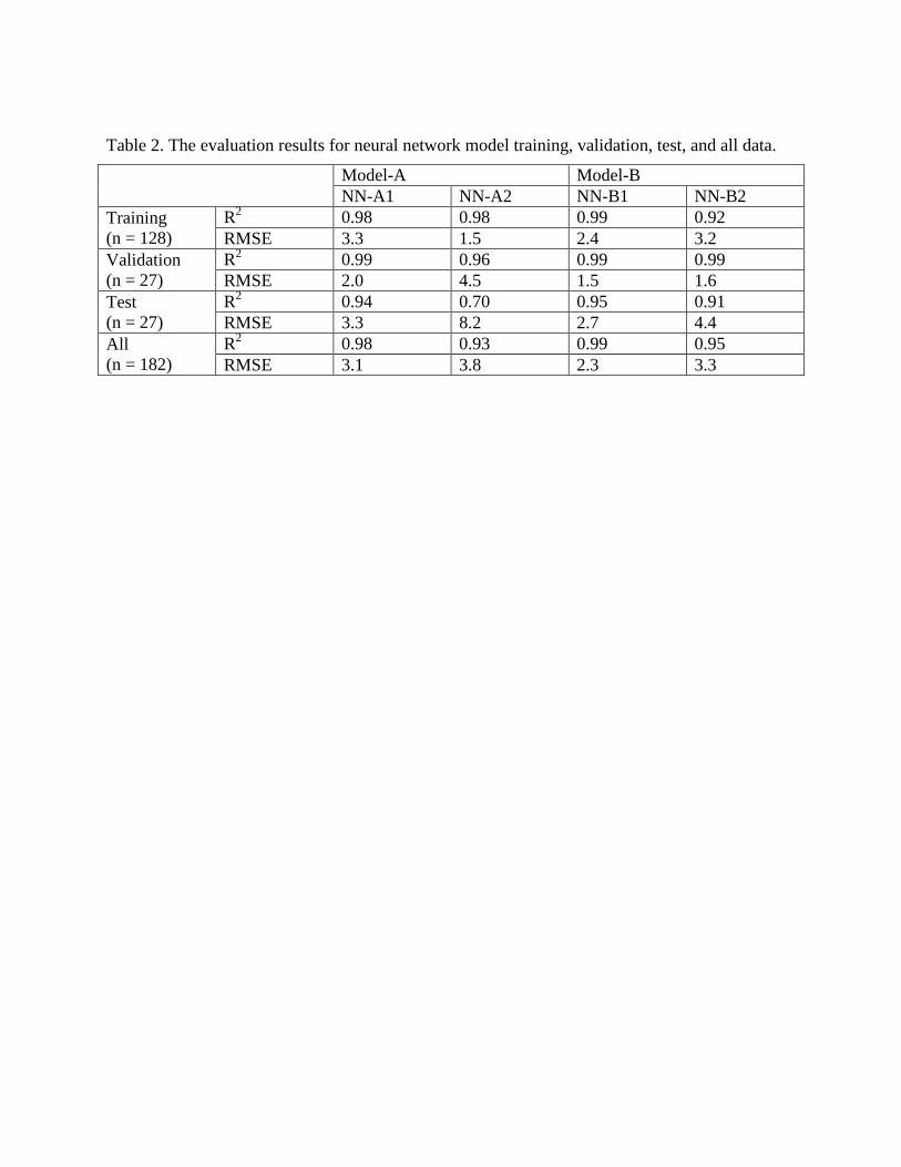
Table 2. The evaluation results for neural network model training, validation, test, and all data.

Model-A Model-B

NN-A1 NN-A2 NN-B1 NN-B2

Training

(n = 128)

R2 0.98 0.98 0.99 0.92

RMSE 3.3 1.5 2.4 3.2

Validation

(n = 27)

R2 0.99 0.96 0.99 0.99

RMSE 2.0 4.5 1.5 1.6

Test

(n = 27)

R2 0.94 0.70 0.95 0.91

RMSE 3.3 8.2 2.7 4.4

All

(n = 182)

R2 0.98 0.93 0.99 0.95

RMSE 3.1 3.8 2.3 3.3

Figure 1. Typical neural network model (INHNO1) for forecasting time series.

Figure 2. Relationship between maximum wind speeds and central pressures in the North Atlantic Ocean.

Figure 3. Relationship between central pressures and radius of maximum wind speed in the North Atlantic Ocean.

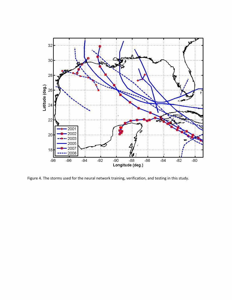
Figure 4. The storms used for the neural network training, verification, and testing in this study.

Figure 5. The comparison between observed and forecasted data of CP and RMW for Model-A.

Figure 6. The comparison between observed and forecasted data of CP and RMW for Model-B.

Figure 7. The hurricanes tracks considered for multiple time step forecasting.

Figure 8. The comparison between observed and forecasted CP and RMW for Hurricane Dennis.

The forecasting was conducted from 7/7/2005 00:00 to 7/11/2005 00:00. The green vertical line

indicates the hurricane’s landfall time.

Figure 9. The comparison between observed and forecasted CP and RMW for Hurricane Katrina.

The forecasting was conducted from 8/26/2005 00:00 to 8/29/2005 18:00. The green vertical line

indicates the hurricane’s landfall time.

Figure 10. The comparison between observed and forecasted CP and RMW for Hurricane Rita.

The forecasting was conducted from 9/20/2005 12:00 to 9/24/2005 12:00. The green vertical line

indicates the hurricane’s landfall time.

Figure 11. The comparison between observed and forecasted CP and RMW for Hurricane

Gustav. The forecasting was conducted from 8/28/2008 18:00 to 9/1/2008 18:00. The green

vertical line indicates the hurricane’s landfall time.

Figure 12. The comparison between observed and forecasted CP and RMW for Hurricane Ida.

The forecasting was conducted from 11/7/2009 18:00 to 11/10/2009 06:00. The green vertical

line indicates the hurricane’s landfall time. The Downward-pointing triangle indicates the

tropical storm stage of Hurricane Ida.

Appendix D

Development and Application of a Simulation Driven

Decision Making Framework (SiDMAF)

1. Introduction

The United States Gulf of Mexico coast ranging from Texas to Florida is vulnerable to

frequent hurricane activities. From 1715 to 1985, approximately forty hurricanes struck in that

region. Over the years, these hurricanes greatly affected the inhabitants surrounding the coast and

resulted in millions of dollars in property damage and hundreds of deaths. Among them, the most

severe hurricanes were the Galveston Hurricane of 1900, the 1935 hurricane that destroyed the

Florida Keys, Hurricane Camille in 1969 and most recently, hurricane Katrina in 2005 which

devastated the Mississippi coast. On the Mississippi coast, Katrina brought about an extreme

surge with maximum elevations on the order of 8-9 meters (Niedoroda et al. 2010).

The devastation of Hurricanes Katrina and Rita in 2005 focused new attention on

predicting storm surges and assessing risks. It is a common practice to use an integrated, coupled

forecasting system for tides, winds and waves to forecast storm surge. Various storm surge

models (i.e., SLOSH, CH3D-SSMS, ADCIRC) have been developed and used in real-time for

estimating storm surge from an approaching hurricane. Even with the advent of super computing

resources, the applications of process based and coupled simulations are often constrained by the

fact that execution of such numerical models is complex and often time consuming.

Once a hurricane is developed in the Atlantic or Pacific oceans, the United States

National Hurricane Center (NHC) releases hurricane advisory data every 6 hours. When a new

hurricane advisory is released, decision makers and emergency managers need crucial

information such as extent and timing of storm surge with sufficient accuracy ahead of the actual

event. In recent years, several techniques have been used to provide such crucial information.

One of the techniques is to run a storm surge model such as ADCIRC using hundreds of

computers (or CPUs) in parallel and use a hotstart concept where the model simulation starts

from the nowcast point representing current conditions (Fleming et al. 2007). Other forecasting

systems use simple equations to reduce computational time for preparing the input data. For

example, using the synthetic asymmetric vortex and wind forcing model (Holland model;

Holland 1980) allows the surge forecasting model to use surface wind and pressure data without

waiting several hours to get these wind data from the National Center for Environmental

Prediction (NCEP) model (Mattocks & Forbes 2008). Even with such various efforts, it can take

hours to forecast storm surge in real time once a hurricane advisory is issued from NHC.

To address these limitations, we have developed and verified an alternative, efficient and

robust data mining technique to forecast storm surge and assess risk in coastal areas. The

developed Simulation Driven Decision Making Framework (SiDMAF) can be used to predict the

extent of storm surge (e.g., maximum surge elevation, inundation area, surface wind and wave

field) and related risk due to coastal inundation. With the help of this tool, decision makers and

emergency managers can quickly assess the impact of an approaching hurricane and make

objective decisions by evaluating what-if-scenarios quickly following each NHC advisory and

starting two to three days ahead of landfall.

2. Background Data

In 2004, the Federal Emergency Management Agency (FEMA) Region Six (FEMA-R6)

initiated a program to update the flood insurance rate maps for the state of Mississippi. Hurricane

Katrina contributed important new data in the area of local climatology and high quality

observations of flood elevation data. FEMA-R6 assigned the task of restudying the Mississippi

coastal areas to a team led by the URS Corporation, and directed it to work closely with related

efforts of the U.S. Army Corps of Engineers (Corps) already underway in the region (Resio et al.

2007; Niedoroda et al. 2010). In the FEMA-R6 study, the historical hurricanes in Gulf of Mexico

were characterized by storm frequency of occurrence, landfall track azimuth (Theta), central

pressure deficit (dp), pressure scale radius (Rp), forward speed (Vf) of the storm and landfall

position. Based on these hurricane characteristics, an optimum sampling method was developed

using Joint Probability Methods (JPM) to find a set of hypothetical synthetic storms to represent

the full range of conditions contained in the historic storm population. Each of the synthetic

storms was then offset by a distance of one radius to maximum wind from the landfall location,

creating multiple offset synthetic tracks that covered the entire length of the Mississippi coast.

Table 1 shows the synthetic storm parameters used in FEMA-R6 study. In the FEMA-R6 study,

228 synthetic storms represented by a unique combination of track, intensity, forward speed,

storm size and radial wind profile decay were considered. A similar approach was also used by

the USACE to develop flood frequency for Eastern Louisiana. USACE developed 47 synthetic

storms which were representative to the coast of Eastern Louisiana. Each of the synthetic storms

was simulated using the Planetary Boundary Layer Model (TC-96) to simulate the translating

wind and pressure fields of hurricanes (Thompson and Cardone 1996); the WAM ocean wave

model (Uniwave 3G) for deep-water waves; the SWAN model (ver. 40.51) for storm waves

approaching the coast (Rogers et al. 2002); and the ADvanced CIRCulation Model (ADCIRC)

for simulations of the storm surge (Westerink and Luettich 1991). All model results of the

combined 275 synthetic storms were then archived as part of the present study. Figure 1 shows

the track distribution of the 275 synthetic storms which made landfall close to the Mississippi

coast.

3. Methodology

The archived 275 high resolution ADCIRC simulations were organized in a central

database in an effort to assess future risks. These were done through an efficient data mining

technique. A Graphical User Interface (GUI) was also developed. The GUI named as SiDMAF

operates in real time and is also capable to validate observed storm surges from historical

hurricanes. For validation, the tool compares simulation results with observed High Water Marks

(HWM) from historical hurricanes (e.g., Camille and Katrina) that made landfall in the Gulf of

Mexico and close to the Mississippi coast. In real time, the SiDMAF tool automatically extracts

hurricane information (e.g., current location, central pressure and radius to maximum wind) from

the NHC website and identifies best matching synthetic storms by establishing a correlation

between the approaching hurricane and synthetic storms within the database.

In the GUI, model validations are achieved by extracting key parameters of the

representative historical hurricanes located in the Best Track information at the NHC website and

then comparing those parameters with the synthetic storms archived in the database. During this

process, three main parameters are compared which are: 1) Landfall location (SLF), 2) Central

pressure (Cp) and 3) Radius to maximum wind (Rmax). The Cp and Rmax parameters are compared

at an offshore location which corresponds to the storm position at a time 8 hours ahead of the

landfall (Niedoroda et al. 2010). With these three major storm parameters, and by comparing

available HWMs associated with the representative historical storms and ADCIRC simulation

results within the database, the toolbox then extracts the best matching synthetic storm. Example

results are demonstrated in the following section.

In real time, the tool operates sequentially. At first, the GUI collects current hurricane

information by accessing the Automated Tropical Cyclone Forecast (ATCF) database provided

by the National Hurricane Center (NHC). Since 2008, the NHC website has been providing real

time GIS coverage of the forecast advisory such as five day hurricane cone. This GIS data from

NHC are utilized by the GUI. The ATCF site also provides possible hurricane tracks and with

maximum sustained wind speed at specific intervals (typically every 6 hours) starting 5 to 7 days

ahead of the landfall. In our approach, the real time GIS data from NHC is used to determine the

projected landfall location (SLF) and the characteristic forward speed (SFS), and storm track

(STRK) of the approaching hurricane. The central pressure (Cp) and radius to maximum wind

(Rmax) values at the current location are also extracted from the NHC official forecast site

(ftp//:ftp.nhc.noaa.gov/atcf/afst/). Normally, the NHC releases real time data, such as position,

Cp, and Rmax as well as the STRK with cone of uncertainty of an approaching hurricane developed

in the Northern Atlantic Basin starting 5 to 7 days ahead of the landfall. The forward speed (SFS)

is estimated by using the information available for the forecasted hurricane track. The evolution

and development of the forecasted track from the NHC along with the information of key

parameters allow the SiDMAF GUI to compare with the characteristics of the synthetic storm

parameters archived in the database. The GUI then identifies a group of storms that best matches

with the track distribution and characteristics of the approaching hurricane. The toolbox uses a

weight based Storm Similarity Index (SSI) to identify the best matching synthetic storm by

correlating hurricane characteristic parameters at a current hurricane position and estimated

landfall location with the characteristics of the synthetic storms within the underlying database.

The SSI ranges from 0 to 1 and is calculated by the following:

SSI = ( a·HLF + b·HCp + c·HRmax + d·HFS ) ·HTRK

where, HLF = parameter indicating landfall similarity (0 to 1); HCp = central pressure similarity (0

to 1); HRmax = pressure scale radius similarity (0 to 1); HFS = storm forwarding speed similarity

(0 to 1); HTRK = storm track similarity (0 or 1), which indicates the similarity for forward

direction of a hurricane. Here, a, b, c, and d = weighting factor whose summation is one. In the

present toolbox, fixed values of a, b, c and d were used which were 0.4, 0.3, 0.2 and 0.1

respectively. These values were optimized for coastal Mississippi.

The simulation process starts with calculating SSI values by correlating current hurricane

position, Cp and Rmax values along with the forecasted track and landfall location (SLF) with the

characteristics of the synthetic storms. Based on the SSI, the toolbox then identifies a group of

storms that closely matches with the characteristics of the approaching hurricane and then

displays ADCIRC simulation results (e.g., maximum surge elevation and hydrographs at specific

locations) in Google Earth environment. This is a very fast process, taking only about 2 to 3

minutes on a regular PC to forecast high resolution storm surge once an advisory is issued by the

NHC. As mentioned earlier, NHC advisories are issued every 6 hours (ftp.nhc.noaa.gov) starting

6-7 days ahead of the projected landfall. However, the current GUI can only be used once the

hurricane enters the Gulf of Mexico and can be operational typically 2-3 days ahead of the

landfall. Once an advisory is issued at the NHC, the SiDMAF GUI operates in an autonomous

mode extracting key data from the advisory, and then comparing those with the synthetic storms

in the database and then displaying key results such as extent and height of storm surge with

hydrographs in Google Earth. The operation repeats itself once a new advisory is issued at the

NHC website.

4. Results

4.1 Model Validation

For validation, model results were compared with the observed High Water Marks

(HWMs) from historical hurricanes including hurricanes Camille (1969) and Katrina (2005).

These were selected as they made landfall close to Mississippi coast. As mentioned earlier, three

parameters (i.e., SLF, Cp, and Rmax) were used as input to the GUI. These three input parameters

were extracted from the Best Track Information available at the NHC archived database. The

toolbox was able to quickly identify the best matching synthetic storms, which was JOS6016D

for hurricane Camille and JOS6018D for hurricane Katrina stored in the database. Table 2 shows

the input parameters to the GUI and results of the matching synthetic storms for hurricane

Camille and Katrina. Figure 3 shows the tracks for Hurricane Camille and Katrina with the best

matching synthetic storms. The comparison of observed HWMs and model simulation results are

also shown in Figure 3.

The comparison results with observed HWMs show that the SiDMAF performs

satisfactorily in hindcasting historical storms. The correlation between observed and modeled

high water marks were reasonable (R2 =0.81 for both Katrina and Camille).

4.2 Model Application

To demonstrate how the SiDMAF toolbox performs in real time, advisory data issued

during hurricane Gustav (August 29-31, 2008) were used. Two advisory data sets (al072008-

5day-020A, and al072008-5day-027A; herein, referred as advisory numbers 20 and 27) were

chosen. Each data set had the projected hurricane track along with current storm location, Cp and

Rmax values. Figure 4 shows the NHC forecasted Hurricane Gustav tracks and cone of

uncertainty for advisory numbers 20 and 27. Figure 4 also shows the best matching synthetic

storms with highest Storm Similarity Index (SSI) values. It can be seen that for the NHC

advisory number 20, synthetic storm JOS6003A had the highest SSI (0.84), whereas, for the

advisory number 27, the SSI was updated and synthetic storm JOS6001A was found to be the

best matching synthetic storm for the current Hurricane Gustav. Table 3 summarizes the results

identifying the group of storms with high SSI values for these two advisories. Note that, due to

significant changes in the Cp values from advisory number 20 to 27 (980 mb reduced to 958 mb),

a new set of synthetic storms were identified by the SiDMAF toolbox. For validation, the model

results for advisory number 27 data were then compared with the observed HWMs (Figure 5). In

general, the model surge elevations extracted from JOS6001A storm are in a reasonable

agreement with the observed HWM(s). The lower correlation results for Gustav might occur for

two reasons, (1) hurricane Gustav made landfall in the Louisiana coast and (2) the current

database of the SiDMAF is impaired with a storm population that concentrates only on the

Mississippi coast. Nevertheless, even with the limitations of the current database, the application

of the Toolbox is promising. Figure 6 shows the forecasting results for Advisory number 27

displayed on the Google Earth.

5. Interactive Vulnerability Mapping with SiDMAF

An efficient method of estimating storm surge using data mining has been developed. The

SiDMAF GUI operates on a regular PC and takes less than 5 minutes to predict high resolution

local storm surge once advisory data are available at the NHC website. The GUI has been

successfully validated against historical hurricanes Camille and Katrina. Also the GUI has been

demonstrated in real time for hurricane Gustav in order to identify the best matching synthetic

storms which make the approach very efficient and robust. The developed toolbox was then used

to identify hotspots in real time by incorporating socioeconomic determinants. Normalized Z-

scores of aggregate vulnerably values are used to identify tracts by vulnerability groups (Very

Low, Low, Intermediate, High, Very High). Final vulnerability score for each tract has been

calculated as an average of the two vulnerability values (Socioeconomic and storm surge). It is

user specific to choose Z-Score ranges to categories census tracts into individual vulnerability

groups, which makes it easy to re-group the tracts into vulnerability groups depending on the

desires. For Z-scores distribution illustrated in Figure 7, tracts with Z-score ≥1.5 and 0.5 < Z-

score < 1.5 are assigned very high and high vulnerability, respectively, while all other tracts are

intermediate to very low vulnerability. Use of Z-scores approach can help determine how close

or far (standard deviations) a selected tract’s vulnerability is distributed compared to the mean

vulnerability of tracts. For example, if Z-score of a tract is -2.0, it indicates that the particular

tract has 2 standard deviations lower vulnerability than the mean vulnerability of tracts in the

study area. Same ranges of Z-scores showed in Figure 7 are used to assign tracts into

vulnerability groups for the study area of coastal MS.

In SiDMAF, an aggregate value of vulnerability for each census block has been

calculated as an average of standardized indicators values normalized between zero and one.

Final vulnerability score for each tract was calculated as average of two vulnerability values

(Socioeconomic and climatological). A thematic vulnerability map illustrating vulnerability of

census tracts is shown in Figure 8. The interpretation of the thematic map is that, during a flood

event, a red or dark brown‐colored census tract would place it at higher risk than the tracts with

light colors. In this particular case, there are 7 census tracts found to be very highly vulnerable

(Z-score ≥1.5), whereas, 20 tracts are found to be highly vulnerable (0.5 ≤ Z-score < 1.5). The

majority of tracts (32) are in the intermediate vulnerability group (-0.5 ≤ Z-score > 0.5), 16 tracts

are in low vulnerability group (-1.5 ≤ Z-score < -0.5) and 16 tracts are in very low vulnerability

group (Z-score < -1.5).

REFERENCES:

Fleming, J.G., C.W. Fulcher, R.A. Luettich, B.D. Estrade, G.D. Allen, and H.S. Winer (2007),

“A real time storm surge forecasting system using ADCIRC”. Estuarine and Coastal Modeling

Congress 2007, 893-912.

Holland, G.J (1980), “An analytic model of the wind and pressure profiles in hurricanes”,

Monthly Weather Review, 108(8):1212-1218.

Mattocks, C. and C. Forbes (2008), “A real-time, event-triggered storm surge forecasting system

for the state of North Carolina”, Ocean Modeling, 25:95-119.

Niedoroda, A.W., D.T.Resio, G.R.Toro, D.Divoky, H.S.Das, and C.W.Reed (2010), “The role of

wave set-up during extreme storms”, Ocean Engineering, 37: 82–90.

Resio, D.T., S.J. Boc, L. Borgman, V. Cardone, A. Cox, W.R. Dally, R.G. Dean, D. Divoky, E.

Hirsh, J.L. Irish, D. Levinson, A. Niedoroda, M.D. Powell, J.J. Ratcliff, V.Stutts, J. Suhada, G.R.

Toro, and P.J. Vickery (2007), “White Paper on Estimating Hurricane Inundation Probabilities”,

Consulting Report prepared by USACE for FEMA.

Rogers, W.E., J.M. Kaihatu, H.A. H. Petit, N. Booij, and L.H. Holthuijsen (2002), “Diffusion

reduction in a arbitrary scale third generation wind wave model”, Ocean Engineering, 29:1357-

1390.

Thompson, E.F. and V.J. Cardone (1996), “Practical modeling of hurricane surface wind fields”,

Journal of Waterway, Port, Coastal, and Ocean Engineering, 122(4):195-205.

Westerink, J.J. and R.A. Luettich (1991), “Tide and storm surge predictions in the Gulf of

Mexico using model ADCIRC-2D”, Report to the U.S. Army Engineer Waterways Experiment

Station, July, 1991.

Table 1. Synthetic storm parameters used in FEMA-R6 study

Storm ID dp (mb) Rp (nmi) Vf (m/s) Theta (deg.)

JOS6001 66.69 18.61 6.047 -38.91

JOS6002 57.17 29.82 6.047 -13.49

JOS6003 49.72 22.93 6.047 -38.92

JOS6004 57.17 10.83 6.047 -13.49

JOS6005 27.17 20.77 6.047 56.66

JOS6006 92.95 14.7 5.943 -12.81

JOS6007 78.59 30.8 6.014 -12.82

JOS6008 78.59 16.56 4.349 47.33

JOS6009 78.59 8.904 6.014 -12.82

JOS6010 78.59 16.56 14.54 -12.86

JOS6011 70.02 17.98 5.943 -12.82

JOS6012 78.59 16.56 4.346 -71.04

JOS6013 128.7 11.66 5.943 -12.81

JOS6014 103.7 25.3 6.014 -12.82

JOS6015 103.7 13.6 4.349 47.33

JOS6016 103.7 7.313 6.014 -12.82

JOS6017 103.7 13.6 14.54 -12.86

JOS6018 94.47 14.53 5.943 -12.82

JOS6019 103.7 13.6 4.346 -71.04

Table 2. Input values of hurricane parameters (landfall location and Cp and Rmax for Hurricane

Camille and Katrina and result of the best matching synthetic storms.

Input Parameters Results

Name Landfall

(lat/lon, o)

Cp

(mb)

Rmax

(nm) Name

Landfall

(lat/lon, o)

Cp

(mb)

Rmax

(nm)

Camille 30.3/-89.2 905 8 JOS6016D 30.1/-89.4 909 7.3

Katrina 29.3/-89.6 905 20 JOS6018D 29.9/-89.4 910 14.5

Table 3. Advisory forecast data from Hurricane Gustav. These data were used in the SiDMAF

GUI in forecasting mode.

Advisory Number al072008_5day_020A al072008_5day_027A

Date 08/30/00:00 08/31/12:00

Location (Lat/Long; o) 19.3/-80.0 29.1/-90.4

Current Cp (mb) 980 958

Current Rmax (nm) 20 15

Landfall Location

(Lat/Long; o)

29.1/-91.0 29.1/-90.4

Results

Synthetic Storm SSI Synthetic Storm SSI

JOS6003A

JOS6001A

JOS6011A

CAT2008A

JOS6003B

CAT2008B

0.84

0.80

0.78

0.77

0.75

0.71

JOS6001A

CAT2008A

JOS6001B

CAT2008B

JOS6004A

CAT2008C

0.82

0.78

0.73

0.72

0.71

0.63

Figure 1. The combined track distribution in FEMA-R6 and USACE studies

(a) Hurricane Camille (b) Hurricane Katrina

Figure 3. Track of Hurricane Camille and Katrina and the best matching synthetic storms

(JOS6016D for Camille and JOS6018D for Katrina).The symbols show the HWM locations and

their comparison with simulated results. Green dots show that the errors between observed and

simulated HWM are less than 1 ft.

(a) Advisory Number 20 and synthetic storm tracks

(b) Advisory Number 27 and synthetic storm tracks

Figure 4. Forecasted Hurricane Gustav tracks (Advisory Number 20 and 27) and synthetic storm

tracks having the high SSI values. (a) for Gustav Advisory 20 and (b) for Gustav Advisory 27.

The blue dots (o) indicate the current hurricane location and the Green line shows the cone of

uncertainty.

Figure 5. Track of Hurricane Gustav (in Red) and the best matching synthetic storm JOS6001A

(in Blue). Green dots show the observed HWMs with errors less than 1 ft.

Figure 6. The forecasting results of Advisory number 27 displayed on the Google Earth. The

color contour indicates the storm surge elevation; Green squares (■) on the map indicates the

stations showing hydrographs (eg., the white box shows a hydrograph at Mississippi River at

Head of Passes)

Figure 7. Use of Z-Scores to Determine Vulnerability

Figure 8. Illustration of Vulnerability of Tracts Developed using Normalized Z-Score

Approach