Design, modeling, simulation and control ofhuman inspired robotic arm

Yao Wang

Abstract

In the traditional industrial robotic field, the mechanical andcontrol systems are usually designed for certain functions. They areplanned to efficiently complete one or several specific tasks, such asgrasping, cutting and assembling. However, it is difficult to extendfunctions based on the industrial robotic hardware platform. Also,the broader applications of robot in the real world involve interactionwith humans. Inspired from human shoulder and arm, we propose asix-degree of freedom robotic arm system. On the basis of the me-chanical design inspired from human arm, it is possible to complete avariety of tasks only changing the control methods rather than hard-ware system. As a demonstration, the system is applied to completethree different family tasks: cutting food, cooking and cleaning thefloor.

1 Introduction

With the development of robotic technology, robots are not only required tocomplete work in industry, but also in family. However, the core concept ofindustry task and family work are quite different. While the industry robotscould efficiently complete a single type of work and repeat hundreds of timesin one day, the family robots are required to do different kinds of work, suchas cleaning floor, cutting food and cooking, for once or twice in one day.As a result, the ability diversity is vital for family robots. Until now, themainstream of family robots on the market is still designed with industrialconcept. IRobot owns the products of vacuum cleaning robot ’Roomba’, floorwashing robot ’Scooba’, pool cleaning robot ’Mirra’, etc. All these products

1

Figure 1: Free Body Diagram.

are single function family robots. Therefore, new kinds of robots for familyenvironment have to be developed.

We are developing a humanoid robotic arm. The robotic arm is com-posed of shoulder, elbow, wrist and manipulator and is expected to completedifferent family work with different control methods. In other words. thisrobotic arm is a hardware platform, which is software-scalable for differentfunctions.

2 Design

Arm is one of the most flexible parts of our body. To design and build ahumanoid robotic arm with thinking in engineering, it is necessary to simplifythe complex biomechanical model of human arm to a more feasible one. Thefree body diagram is show in Fig. 1. Fig. 1 shows that the human armmodel here is simplified as a 6 degrees of freedom mechanical system. First,the shoulder part is capable of rotating around the three axes in the Cartesianspace, which contains three degrees of freedom. Second, the elbow indicatesone degree of freedom. Third, the forearm could rotate around the axis

2

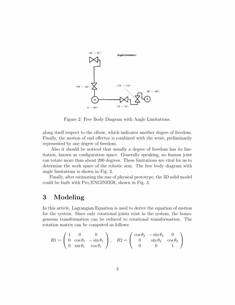
Figure 2: Free Body Diagram with Angle Limitations.

along itself respect to the elbow, which indicates another degree of freedom.Finally, the motion of end effector is combined with the wrist, preliminarilyrepresented by one degree of freedom.

Also it should be noticed that usually a degree of freedom has its lim-itation, known as configuration space. Generally speaking, no human jointcan rotate more than about 200 degrees. These limitations are vital for us todetermine the work space of the robotic arm. The free body diagram withangle limitations is shown in Fig. 2.

Finally, after estimating the size of physical prototype, the 3D solid modelcould be built with Pro/ENGINEER, shown in Fig. 3.

3 Modeling

In this article, Lagrangian Equation is used to derive the equation of motionfor the system. Since only rotational joints exist in the system, the homo-geneous transformation can be reduced to rotational transformation. Therotation matrix can be computed as follows:

R1 =

1 0 00 cos θ1 − sin θ10 sin θ1 cos θ1

, R2 =

cos θ2 − sin θ2 00 sin θ2 cos θ20 0 1

3

Figure 3: 3D Solid Model.

4

R3 =

cos θ3 0 sin θ30 1 0

− sin θ3 0 cos θ3

, R4 =

cos θ4 − sin θ4 00 sin θ4 cos θ40 0 1

R5 =

cos θ5 0 sin θ50 1 0

− sin θ5 0 cos θ5

, R6 =

cos θ6 − sin θ6 00 sin θ6 cos θ60 0 1

define i =

100

, j =

010

, k =

001

, Φ =

000

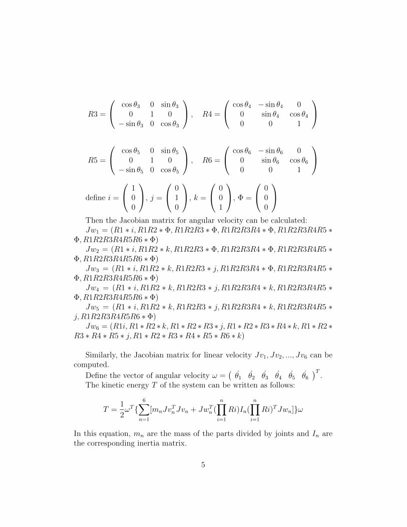
Then the Jacobian matrix for angular velocity can be calculated:Jw1 = (R1 ∗ i, R1R2 ∗ Φ, R1R2R3 ∗ Φ, R1R2R3R4 ∗ Φ, R1R2R3R4R5 ∗

Φ, R1R2R3R4R5R6 ∗ Φ)Jw2 = (R1 ∗ i, R1R2 ∗ k,R1R2R3 ∗ Φ, R1R2R3R4 ∗ Φ, R1R2R3R4R5 ∗

Φ, R1R2R3R4R5R6 ∗ Φ)Jw3 = (R1 ∗ i, R1R2 ∗ k,R1R2R3 ∗ j, R1R2R3R4 ∗ Φ, R1R2R3R4R5 ∗

Φ, R1R2R3R4R5R6 ∗ Φ)Jw4 = (R1 ∗ i, R1R2 ∗ k,R1R2R3 ∗ j, R1R2R3R4 ∗ k,R1R2R3R4R5 ∗

Φ, R1R2R3R4R5R6 ∗ Φ)Jw5 = (R1 ∗ i, R1R2 ∗ k,R1R2R3 ∗ j, R1R2R3R4 ∗ k,R1R2R3R4R5 ∗

j, R1R2R3R4R5R6 ∗ Φ)Jw6 = (R1i, R1 ∗R2 ∗ k,R1 ∗R2 ∗R3 ∗ j, R1 ∗R2 ∗R3 ∗R4 ∗ k,R1 ∗R2 ∗

R3 ∗R4 ∗R5 ∗ j, R1 ∗R2 ∗R3 ∗R4 ∗R5 ∗R6 ∗ k)

Similarly, the Jacobian matrix for linear velocity Jv1, Jv2, ..., Jv6 can becomputed.

Define the vector of angular velocity ω =(θ1 θ2 θ3 θ4 θ5 θ6

)T.

The kinetic energy T of the system can be written as follows:

T =1

2ωT{

6∑n=1

[mnJvTnJvn + JwTn (

n∏i=1

Ri)In(n∏i=1

Ri)TJwn]}ω

In this equation, mn are the mass of the parts divided by joints and In arethe corresponding inertia matrix.

5

Then the potential energy could be computed as:

V =(

0 −1 0)∗

6∑n=1

(mnpn) ∗ g

In this formula, pn is the mass center of different parts and g is theacceleration of gravity.

The motion of equation can be got by substituting T and V into La-grangian equation:

d

dt(∂L

∂θi)− ∂L

∂θi= τ

In this equation, L = T − V , τ is the generalized force.Finally, the motion of equation can be written as following format:

M(θ)θ + C(θ, θ)θ +N(θ, θ) = τ

4 Simulation

In this article, ADAMS is selected as the simulation environment. ADAMSprovides several numerical methods for simulation. Here the default integra-tor GSTIFF is chosen. It is a stiffly stable, multi-step, variable order andvariable step integrator and is fast and accurate for computing displacementsfor a wide range of motion analysis problems. As a backward difference for-mulation, the general form of GSTIFF could be written as follows:

yn+1 =k∑

1=1

αiyn−i+1 + hβ0y′

n+1

In the simulation, the order of the integrator is up to five. Then the formu-lations are shown as follows:

1storder : yn+1 = yn + hy′n+1

2ndorder : yn+1 = 43yn − 1

3yn−1 + 2

3hy

′n+1

3rdorder : yn+1 = 1811yn − 9

11yn−1 + 2

11yn−2 + 6

11hy

′n+1

4thorder : yn+1 = 4825yn − 36

25yn−1 + 16

25yn−2 − 3

25yn−3 + 12

25hy

′n+1

5thorder : yn+1 = 300137yn− 300

137yn−1+ 200

137yn−2− 75

137yn−3+ 12

137yn−4+ 60

137hy

′n+1

Test single joint input in ADMAS and apply a harmonic excitation onthe first joint, the response is shown in Fig. 4 to Fig. 9:

6

Figure 4:

Figure 5:

Figure 6:

7

Figure 7:

Figure 8:

Figure 9:

8

5 Control Design

5.1 Motion Planning

Some family tasks, such as mopping the floor and cooking, share some com-mon features. In the process of completing these tasks, several joints ofhuman’s arm sustain fixed angles and other joints move in periodic style,such as harmonic motion. These features are basis for more complex trajec-tory in the future application. Here the motion planning of mopping floor isexecuted as an example.

Through examining the actual gesture of human when mopping the floor,the third and fifth joints are set to sustain fix angles in the mopping process.Define θi, ωi and βi as the rotation angle, angular velocity and angular accel-eration of each joint.(i = 1, 2, ..., 6) Then the parameters of fixed joints canbe written as follows:

θ3 = 0; ω3 = 0; β3 = 0.

θ5 =π

2; ω5 = 0; β5 = 0.

Through geometric analysis, parameters of the first, second, fourth andsixth joints can be determined. The geometric relation of θ2 and θ4 is shownin Fig. 10

The range of θ4 is from 0◦ to 114.55◦, then it can be defined as follows:

θ1 =π

4+

π

12cos(

π

2t)

In the Fig. 10, length of AB and BC are the length of forearm and arm.They are determined by the design parameters. The length of AC here canbe computed as follows:

|AC| = (|AB|+ |BC|)2 cos θ1

As a result, θ2 can be calculated from the following equation:

sin(θ4 − θ2)|BC|

=sin θ2|AB|

Similarly, the following equation can be used to obtain θ1 if θ2 is known:

9

Figure 10: Geometric Analysis.

{|AC| = (|AB|+|BC|)

2 cos θ1, ;

sin(θ4|AC| = sin θ2

|AB| , .

Finally, θ6 can be derived from θ1:

θ6 =π

2− θ1

Additionally, the angular velocities and angular accelerations can be com-puted from the angle function:

ωi =dθidt

βi =dωidt

(i = 1, 2, ..., 6)

As a result, the motion trajectory of the robotic arm can be completelydetermined for the task of mopping floor.

Although the trajectory design for the working process has been com-pleted, the motion planning problem can be more complicated if the initialcondition is taken into consideration. Assume that the robotic arm is at restinitially.(The angles, angular velocities and angular accelerations are all zero)However, the initial conditions of the working trajectory is not all-zero. In

10

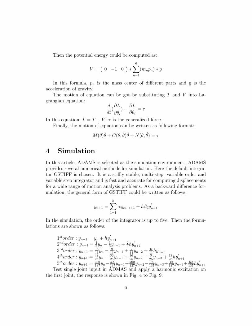
other words, there would be some ”step stage” for several kinetic parametersof system. The total function of these parameters versus time is discontin-uous at initial time, which affects the response and produces overshoots oroscillations. Since the robotics arm would work in the family environment,the ”extra action” is not expected for safety of human. To eliminate these”extra actions”, it is necessary to find the kinetic parameters of which theinitial conditions are not satisfied with the function value of working trajec-tory at time zero. To solve this problem, an extra stage of ”lift” is designed,to set the initial conditions of certain joints to the desired values over twoseconds. Then the angle functions of all the joints can be written as follows:

θ1 = − π

12t3 +

π

4t2; θ2 = 0;

θ3 = 0; θ4 = 0;

θ5 = −π8t3 +

3π

8t2; θ2 =

π

24t3 − π

8t2;

Then the whole motion planning is finished.

5.2 Trajectory Tracking

5.2.1 Computed Torque Method

The dynamics of the robotic arm can be expressed in the following form:

M(θ)θ + C(θ, θ)θ +N(θ, θ) = τ

Given a desired joint trajectory θd(·), assume that the model is preciseand initial conditions are exactly the same:

θ(0) = θd(0); θ(0) = θd(0)

The control torque can be chosen as follows:

τ = M(θd)θd + C(θd, θd)θd +N(θd, θd)

Since θ and θd have the same initial conditions and satisfies the samedifferential equation, then from the uniqueness of differential equation it canbe shown that θ(t) = θd(t) for all t ≥ 0).

11

This is an open-loop control law and the robustness cannot be ensured.Here a state feedback is added into the control law:

τ = M(θd)θd + C(θd, θd)θd +N(θd, θd)− F (Kve+Kpe)

In this equation, Kp and Kv are proportional and derivative coefficient ma-trices. They are both constant matrices. F is a time-varying matrix to dedetermined. However, the motion equation of the system should be linearizedaround the designed trajectory before the specific structures and values ofmatrices Kp, Kv and F can be determined. It is assumed that the error be-tween actual motion and desired trajectory is small enough throughout thewhole process of movement. Then the nolinear parts in the equation can belinearized as follows:

M(θ) = M(θd); C(θ, θ) = C(θd, θd); N(θ, θ) = N(θd, θd)

It follows that:

M(θd)e+ [C(θd, θd) + FKv]e+ FKpe = 0

Then the robotic arm model is converted to a linear time-varying system,Since the initial conditions are ensured that e(0) = e(0) = 0, the objectiveis to make the system internally stable through selecting appropriate F , Kp

and Kv, to guarantee that e(t) = e(t) = 0 for all t ≥ 0.From the linear control theory, it is known that a time-varying equation

is asymptotically stable if

‖Φ(t, t0)‖ −→ 0 as t −→∞

for all t, t0 with t ≥ t0. Φ(t, t0) is the transition matrix.One procedure of selecting the matrices F , Kp and Kv is as follows:(1) Write the matrix F to be a diagonal matrix with the diagonal elements

as the diagonal elements of the matrix M(θd).(2)Select appropriate constant diagonal matrices Kp and Kv to make the

system track the desired trajectory.(3)Adjust Kp and Kv to eliminate the oscillation and errors.Through this design procedure, some tasks and applications which don’t

require to move very fast can be completed. The simulation result of atrajectory concerning harmonic motion is shown in Fig. 11.

12

Figure 11: Simulation Result.

13

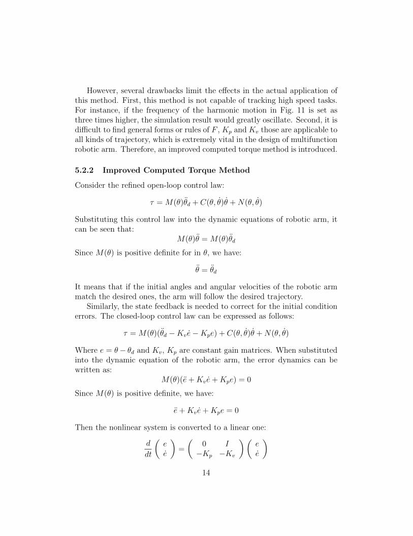
However, several drawbacks limit the effects in the actual application ofthis method. First, this method is not capable of tracking high speed tasks.For instance, if the frequency of the harmonic motion in Fig. 11 is set asthree times higher, the simulation result would greatly oscillate. Second, it isdifficult to find general forms or rules of F , Kp and Kv those are applicable toall kinds of trajectory, which is extremely vital in the design of multifunctionrobotic arm. Therefore, an improved computed torque method is introduced.

5.2.2 Improved Computed Torque Method

Consider the refined open-loop control law:

τ = M(θ)θd + C(θ, θ)θ +N(θ, θ)

Substituting this control law into the dynamic equations of robotic arm, itcan be seen that:

M(θ)θ = M(θ)θd

Since M(θ) is positive definite for in θ, we have:

θ = θd

It means that if the initial angles and angular velocities of the robotic armmatch the desired ones, the arm will follow the desired trajectory.

Similarly, the state feedback is needed to correct for the initial conditionerrors. The closed-loop control law can be expressed as follows:

τ = M(θ)(θd −Kve−Kpe) + C(θ, θ)θ +N(θ, θ)

Where e = θ− θd and Kv, Kp are constant gain matrices. When substitutedinto the dynamic equation of the robotic arm, the error dynamics can bewritten as:

M(θ)(e+Kve+Kpe) = 0

Since M(θ) is positive definite, we have:

e+Kve+Kpe = 0

Then the nonlinear system is converted to a linear one:

d

dt

(ee

)=

(0 I−Kp −Kv

)(ee

)14

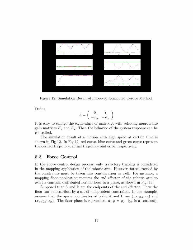
Figure 12: Simulation Result of Improved Computed Torque Method.

Define

A =

(0 I−Kp −Kv

)It is easy to change the eigenvalues of matrix A with selecting appropriategain matrices Kv and Kp. Then the behavior of the system response can becontrolled.

The simulation result of a motion with high speed at certain time isshown in Fig 12. In Fig 12, red curve, blue curve and green curve representthe desired trajectory, actual trajectory and error, respectively.

5.3 Force Control

In the above control design process, only trajectory tracking is consideredin the mopping application of the robotic arm. However, forces exerted bythe constraints must be taken into consideration as well. For instance, amopping floor application requires the end effector of the robotic arm toexert a constant distributed normal force to a plane, as shown in Fig. 13.

Supposed that A and B are the endpoints of the end effector. Then thefloor can be described by a set of independent constraints. In our example,assume that the space coordinates of point A and B are (xA, yA, zA) and(xB, yB, zB). The floor plane is represented as y = y0. (y0 is a constant).

15

Figure 13: Mopping Floor.

Then the surface constraints can be written as:{h1(θ1, θ2, ..., θ6) = yA(θ1, θ2, ..., θ6)− y0 = 0h2(θ1, θ2, ..., θ6) = yB(θ1, θ2, ..., θ6)− y0 = 0

Now the floor surface is represented as the function h of the generalizedcoordinates θ1, θ2, ..., θ6. Hence, the normal vectors to this surface are givenby the span of the gradients of ∇h. As a result, any torques with the form

τN =∑

λj∇hj

correspond to normal forces applied against the floor surface. If the friction isnot taken into consideration, the work done by these torques can be computedas follows:

τN · θ =∑

λj∇hj · θ =∑

λj(∂hj∂θ

θ)

=∑

λjdh

dt= 0

It means that the normal forces have no effect on the motion of the roboticarm. In the previous trajectory tracking parts, the computed torque τ has beattained to follow the desired motion. Now if we consider the force control,the complete control law is given by:

τc = τ + τN

Since the torques τN do not affect the trajectory tracking part, their functionis to exert desired forces to the floor surface.

16

6 Summary

In this article, modeling of the robotic arm is completed with Lagrangianmethod. Then the simulation of the system motion is base on the GS-TIFF numerical method. In the control design method, the computed torquemethod is first used for trajectory tracking. However, due to the limitation ofapplication in the high speed motion, the improved torque method is intro-duced for the position control. Finally, the basic force control is introducedto deal with the environmental forces. In the future work, control strategiesfor the system with the actuators, such as motors and sensors, should bedeveloped for the actual application. Also the physical prototype would bebuilt in the future.

References

[1] M. Tomsic N. Klopcar and J. Lenarcic. A kinematic model of the shoul-der complex to evaluate the arm-reachable workspace. Journal of Biome-chanics, 40:86–91, 2007.

[2] Goran Sigholm Christian Hogfors and Peter Herberts. Biomechanicalmodel of the human shoulder-i. elements. Journal of Biomechanics,20:157–166, 1987.

[3] Mahmoud A. Moustafa Khaled T. Mohamed, Shihab S. Asfour andHasan A. Elgamal. A computerized dynamic biomechanical model ofthe human shoulder complex. Computers ind. Engng, 31:503–506, 1996.

[4] Walter Maurel and Daniel Thalmann. Human shoulder modeling in-cluding scapulo-thoracic constraint and joint sinus cones. Computersand Graphics, 24:203–218, 2000.

[5] H. Bao and P.Y. Willems. On the kinematic modelling and the pa-rameter estimation of the human shoulder. Journal of Biomechanics,32:943–950, 1999.

[6] DAN KARLSSON and BO PETERSO. Towards a model for force pre-dictions in the human shoulder. Journal of Biomechanics, 25:189–199,1992.

17

[7] Guangpin He Xiguang Huang and Duanling Li. Kinematics analysisof a parallel robotic manipulator. Applied Mechanics and Materials,29–32:956–960, 2010.

[8] Xiaoping Su Dan Zhang, Jijie Qian and Zhen Gao. Design, analysis andfabrication of a novel three degrees of freedom parallel robotic manipu-lator with decoupled motions. Int J Mech Mater, 9:199–212, 2013.

[9] Anjan Kumar Swain and Alan S. Morris. A united dynamic model for-mulation for robotic manipulator systems. Journal of Robotic Systems,20:601–620, 2003.

[10] Thomas R. Kane and David A. Levinson. DYNAMICS: Theory andApplications. McGraw-Hill Book Company, 1985.

[11] Seth Hutchinson Mark W. Spong and Mathukumalli Vidyasagar. RobotModeling and Control. Wiley, 2005.

[12] Zexiang Li Richard M. Murray and S. Shankar Sastry. A MathematicalIntroduction to Robotic Manipulation. CRC Press, 1994.

[13] Kemin Zhou. ESSENTIALS OF ROBUST CONTROL. PRENTICEHALL, 1999.

18

Appendix

Name Quantity Website Cost($

)

Twin Geared

Motor- Tamiya

70097

3 http://www.robotmarketplace.com/products/0-70097.htm

l

35.1

Kitbots 1000

RPM Gearmotor

3 http://www.robotmarketplace.com/products/KB-1000RP

M.html

48

Pololu Dual DC

Motor Driver 1A,

4.5V-13.5V-

TB6612FNG

3 http://www.robotshop.com/en/pololu-dual-dc-motor-driv

er-1a-4-5v-3-5v-tb6612fng.html

14.85

Arduino Due

32bit ARM

Microcontroller

1 http://banebots.com/pc/WHB-HM-HS6-S4/T82H-SS42 49.95

AS Series 360°

3.3 to 5 V SMT

Programmable

Magnetic Rotary

Encoder -

SSOP-16

6 http://www.futureelectronics.com/en/technologies/semic

onductors/analog/sensors/gyro-angular-rate/Pages/36503

14-AS5045-ASST.aspx?IM=0

36.42

BMI055 Series

3.6 V 5 mA Small

Veratile 6 DoF

Sensor Module -

6 http://www.futureelectronics.com/en/Technologies/Produ

ct.aspx?ProductID=BMI0550273141134BOSCH7035254&I

M=0

20

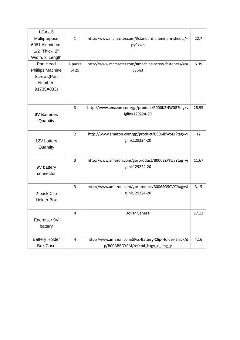
LGA-16

Multipurpose

6061 Aluminum,

1/2" Thick, 2"

Width, 3' Length

1 http://www.mcmaster.com/#standard-aluminum-sheets/=

py9kwq

22.7

Pan Head

Phillips Machine

Screws(Part

Number:

91735A833)

1 packs

of 25

http://www.mcmaster.com/#machine-screw-fasteners/=m

c86h3

6.39

9V Batteries

Quantity

3 http://www.amazon.com/gp/product/B000K2NW08?tag=v

iglink129224-20

28.95

12V battery

Quantity

2 http://www.amazon.com/gp/product/B006IBWSLY?tag=vi

glink129224-20

12

9V battery

connector

3 http://www.amazon.com/gp/product/B0002ZPFU8?tag=vi

glink129224-20

11.67

2-pack Clip

Holder Box

3 http://www.amazon.com/gp/product/B006SQ50VY?tag=vi

glink129224-20

3.15

Energizer 9V

battery

4 Dollar General 17.12

Battery Holder

Box Case

4 http://www.amazon.com/5Pcs-Battery-Clip-Holder-Black/d

p/B00ABRQYPM/ref=pd_bxgy_e_img_y

4.16