Report 08-01 Temblor Pisco Peru
159
-
Upload
drsalgadouagro -
Category
Documents
-
view
4 -
download
0
description
Reporte de daños por el sismo de Perú del2007
Transcript of Report 08-01 Temblor Pisco Peru


The Pisco-Chincha Earthquake of August 15, 2007 Seismological, Geotechnical, and Structural Assessments
Amr S. Elnashai Jorge Alva-Hurtado
Omar Pineda Oh Sung Kwon
Luis Moran-Yanez Guillermo Huaco
Gregory Pluta
Mid-America Earthquake Center
MAE Center Report 08-01 Civil and Environmental Engineering Department November 2008 University of Illinois at Urbana – Champaign Urbana, Illinois 61801, UNITED STATES +1 217 244 6302, [email protected]
Epicenter(13.32° S 76.51° W)
Lima (150 km)
ICA (115 km)
Pisco (51 km)
Chincha Alta(42 km)
50 km
100 km
150 km
Tampo de Mora (37 km)

1
EXECUTIVE SUMMARY
On August 15, 2007, a strong earthquake of magnitude 8.0 ± 0.1 hit the coastal region of Central Peru, causing considerable loss of life and livelihood. The earthquake was attributed to the highly active source created by the subduction of the Nazca oceanic plate underneath the South American continental plate. The earthquake mechanism was complex with two major ruptures ~60 seconds apart. The earthquake caused about 600 deaths with several hundreds of injuries, destroyed over 50,000 buildings and damaged over 20,000. Extensive soil liquefaction was observed in the coastal planes where houses, utility and communication networks suffered extensive damage due to large permanent ground deformation. Major landslides and evidence of liquefaction were observed in the affected region. On the whole, soil effects and geotechnical consequences were a major feature of this earthquake and lead to extensive damage to foundations, sub-surface and surface structures. Analysis of the strong-motion and its correlation with the seismological characteristics of the earthquake shows that the damage was compounded by the long duration of shaking which resulted from the complex rupture process that lead to a shaking duration of over 120 seconds. Detailed analysis of attenuation characteristics and available strong-motion models shows considerable variation. The attenuation investigation presented in the report emphasizes the case for specific and rigorous studies for regions such as the subduction of Nazca-South America where earthquakes of complex mechanisms may occur. Such earthquakes may not be on the subduction surface, but may originate from the overriding plate. Analysis of the available strong-motion records indicate that higher-than-usual ductility demands were imposed on the exposed civil engineering works, and that the high demand was in a relatively wide range of periods, especially in the East-West direction. Moreover, energy flux analysis of the records indicate a level of energy release many times that from comparable-size earthquakes that have caused substantial damage in recent years. The majority of structural failures were in clay and brick masonry structures. However, several reinforced concrete structures also suffered major damage or collapse, often due to soft storey effects and lack of vertical continuity. The lack of ductile detailing was clear and repetitive even in modern construction. As noted above, in many cases the damage was a consequence of large differential settlement and foundation failure. In conclusion the Pisco-Chincha earthquake occurred in a region of known high seismicity that has been hit many times in the past several hundred years. It has however caused extensive damage that has revealed the critical importance of foundation design to resist large differential settlements in regions of liquefaction susceptibility. The earthquake also underlines the importance of city planning to avoid building in areas susceptible to liquefaction. The extensive damage inflicted on masonry structures emphasizes the case for retrofitting of unreinforced masonry in regions of high seismicity, whilst the damage to RC structures reiterates the known requirements for continuity and uniformity in the lateral force resisting system, and ductile detailing.

2
TABLE OF CONTENTS
EXECUTIVE SUMMARY ................................................................................................................................... 1
LIST OF FIGURES ............................................................................................................................................... 4
LIST OF TABLES ................................................................................................................................................. 7
1 OVERVIEW ................................................................................................................................................. 8 1.1 MACRO-SEISMIC DATA ......................................................................................................................... 8 1.2 DAMAGE AND CASUALTIES DATA ......................................................................................................... 8 1.3 FIELD MISSION ITINERARY .................................................................................................................... 9
2 ENGINEERING SEISMOLOGY ............................................................................................................. 11 2.1 LOCAL GEOLOGY AND TECTONICS ...................................................................................................... 11 2.2 BRIEF HISTORY OF EARTHQUAKES IN THE REGION ............................................................................. 13 2.3 THE PISCO-CHINCHA EARTHQUAKE .................................................................................................... 18
2.3.1 General Information and Rupture Models ..................................................................................... 18 2.3.2 Comparison of Resulting Intensity with Previous Earthquakes ..................................................... 19
3 GROUND MOTION ESTIMATION IN CENTRAL PERU .................................................................. 20 3.1 GROUND MOTION MODELS ................................................................................................................. 20
3.1.1 Information from Seismic Stations ................................................................................................ 20 3.1.2 Estimation of Peak Ground Acceleration with the NGA-CB Model ............................................. 21 3.1.3 Comparison of Computed and Recorded PGA Values .................................................................. 26
3.2 GROUND MOTION MAPS FOR CENTRAL PERU ..................................................................................... 33 3.3 DISCUSSION AND CONCLUSIONS .......................................................................................................... 47
4 STRONG-MOTION DATA ANALYSIS ................................................................................................. 48 4.1 STRONG-MOTION STATIONS AND RECORDS ......................................................................................... 48 4.2 ELASTIC AND INELASTIC SPECTRA ...................................................................................................... 49 4.3 ENERGY FLUX AND INTENSITY MEASURES ......................................................................................... 51 4.4 SELECTION OF ADDITIONAL RECORDS FOR ANALYSIS ........................................................................ 53
5 GEOTECHNICAL ASPECTS .................................................................................................................. 56 5.1 GEOLOGY AND SITE CONDITIONS ........................................................................................................ 56
5.1.1 Geology of Cañete, Jahuay, Chincha and Tambo de Mora ............................................................ 56 5.1.2 Geology of the Huamani Bridge, Pisco, Paracas and Ica ............................................................... 57
5.2 DAMAGE TO FOUNDATIONS ................................................................................................................. 61 5.3 FREE FIELD LIQUEFACTION EFFECTS ................................................................................................... 64
6 STRUCTURAL ENGINEERING ASPECTS .......................................................................................... 69 6.1 REGIONAL DAMAGE DESCRIPTION AND STATISTICS ........................................................................... 69
6.1.1 Pisco ............................................................................................................................................... 69 6.1.2 Tambo de Mora and Chincha Alta ................................................................................................. 83 6.1.3 Ica .................................................................................................................................................. 87
6.2 EFFECT ON LIFE LINES ........................................................................................................................ 90 6.2.1 Damaged Electricity Poles ............................................................................................................. 90 6.2.2 Road Failure ................................................................................................................................... 93 6.2.3 Bridge Failure ................................................................................................................................ 95
6.3 REINFORCED CONCRETE STRUCTURES ................................................................................................ 96 6.3.1 Introduction .................................................................................................................................... 96 6.3.2 Description of Materials, Construction and Systems ..................................................................... 96 6.3.3 Observed Damage Patterns and Implications ................................................................................. 96 6.3.4 Peruvian Code NTE E.030 ........................................................................................................... 105
7 CASE STUDY: ICA UNIVERSITY BUILDING ANALYSIS ............................................................. 106

3
7.1 LOCATION AND RECORDED GROUND MOTION .................................................................................. 106 7.2 CONFIGURATION OF THE REFERENCE BUILDING ............................................................................... 107 7.3 OBSERVED DAMAGE AND CAUSES .................................................................................................... 109
7.3.1 Short Column Effects due to Infill Walls ..................................................................................... 110 7.3.2 Inappropriate Stirrups .................................................................................................................. 111 7.3.3 Overload on the Second Floor ..................................................................................................... 113
7.4 BACK ANALYSIS OF THE REFERENCE STRUCTURE ............................................................................. 114 7.4.1 Analytical Model ......................................................................................................................... 114 7.4.2 Pushover Analysis ........................................................................................................................ 120 7.4.3 Inelastic Response History Analyses ........................................................................................... 121
7.5 CONCLUDING OBSERVATIONS FROM THE ANALYSIS ......................................................................... 123
8 SUMMARY AND RECOMMENDATIONS ......................................................................................... 125 8.1 SUMMARY OF OBSERVATIONS AND LESSONS LEARNED ...................................................................... 125 8.2 RECOMMENDATIONS ......................................................................................................................... 127
8.2.1 Hazard .......................................................................................................................................... 127 8.2.2 Planning for Risk Management .................................................................................................... 127 8.2.3 Design and Construction .............................................................................................................. 127 8.2.4 Legislation ................................................................................................................................... 128
9 ACKNOWLEDGEMENTS ..................................................................................................................... 129
10 REFERENCES ......................................................................................................................................... 130
APPENDIX A ..................................................................................................................................................... 133 A.1 FIELD MISSION MEMBERS AND SPECIALIZATION ...................................................................................... 133 A.2 PERUVIAN HOST ORGANIZATIONS ............................................................................................................ 133 A.3 ITINERARY AND ROUTE ............................................................................................................................. 134
APPENDIX B ..................................................................................................................................................... 136 B.1 RECORDED GROUND MOTIONS AND RESPONSE SPECTRA ............................................................................ 136

4
LIST OF FIGURES FIGURE 1.1 EPICENTER OF THE PISCO-CHINCHA EARTHQUAKE AND AFFECTED CITIES ............................................ 8 FIGURE 1.2 GPS TRAVEL LOG OF THE ENTIRE SITE VISIT ........................................................................................ 10 FIGURE 2.1 CONSTITUENTS OF SUBDUCTION REGIONS ARE DEPICTED .................................................................... 11 FIGURE 2.2 MACRO-TECTONICS OF PERU .............................................................................................................. 12 FIGURE 2.3 SEISMICITY MAP (JANUARY 1900 – JUNE 2001) .................................................................................. 15 FIGURE 2.4 SUPERFICIAL SEISMICITY OF PERU (JANUARY 1900 – JUNE 2001) ....................................................... 16 FIGURE 2.5 SUPERFICIAL INTERMEDIATE SEISMICITY FOR PERU (JANUARY 1900 – JUNE 2001) ............................ 17 FIGURE 2.6 FAULT PLANE SOLUTION AND AFTERSHOCK DISTRIBUTION ................................................................. 19 FIGURE 3.1 FAULT PLANE – PROFILE VIEW ............................................................................................................. 22 FIGURE 3.2 VARIABILITY OF PGA WITH RESPECT TO VS30 AND Z2.5 FOR ICA ......................................................... 25 FIGURE 3.3 VARIABILITY OF PGA WITH RESPECT TO VS30 AND Z2.5 FOR LIMA CITY .............................................. 26 FIGURE 3.4 MAP OF ESTIMATED PGA FOR ROCK SITES (NGA-CB PARAMETER A1110) ........................................... 28 FIGURE 3.5 PGA MAP FOR SITE CLASS B (VS30=1070 M/S) .................................................................................... 29 FIGURE 3.6 PGA MAP FOR SITE CLASS C (VS30=525 M/S) ...................................................................................... 30 FIGURE 3.7 PGA MAP FOR SITE CLASS D (VS30=255 M/S) ..................................................................................... 31 FIGURE 3.8 PGA MAP FOR SITE CLASS E (VS30=150 M/S) ...................................................................................... 32 FIGURE 3.9 MAP FOR ROCK (VS30=1110 M/S) – NGA-CB VARIABLE A1110 ............................................................ 34 FIGURE 3.10 PGA MAP FOR SITE CLASS B (VS30=1070 M/S) AND Z2.5=0.5 KM ...................................................... 35 FIGURE 3.11 PGA MAP FOR SITE CLASS B (VS30=1070 M/S) AND Z2.5=2.0 KM ...................................................... 36 FIGURE 3.12 PGA MAP FOR SITE CLASS B (VS30=1070 M/S) AND Z2.5=3.5 KM ...................................................... 37 FIGURE 3.13 PGA MAP FOR SITE CLASS C (VS30=525 M/S) AND Z2.5=0.5 KM ........................................................ 38 FIGURE 3.14 PGA MAP FOR SITE CLASS C (VS30=525 M/S) AND Z2.5=2.0 KM ........................................................ 39 FIGURE 3.15 PGA MAP FOR SITE CLASS C (VS30=525 M/S) AND Z2.5=3.5 KM ........................................................ 40 FIGURE 3.16 PGA MAP FOR SITE CLASS D (VS30=255 M/S) AND Z2.5=0.5 KM ........................................................ 41 FIGURE 3.17 PGA MAP FOR SITE CLASS D (VS30=255 M/S) AND Z2.5=2.0 KM ........................................................ 42 FIGURE 3.18 PGA MAP FOR SITE CLASS D (VS30=255 M/S) AND Z2.5=3.5 KM ........................................................ 43 FIGURE 3.19 PGA MAP FOR SITE CLASS E (VS30=150 M/S) AND Z2.5=0.5 KM ......................................................... 44 FIGURE 3.20 PGA MAP FOR SITE CLASS E (VS30=150 M/S) AND Z2.5=2.0 KM ......................................................... 45 FIGURE 3.21 PGA MAP FOR SITE CLASS E (VS30=150 M/S) AND Z2.5=3.5 KM ......................................................... 46 FIGURE 4.1 RECORDED ACCELERATIONS FROM ICA2 STATION.............................................................................. 49 FIGURE 4.2 RESPONSE SPECTRUM OF RECORDED ACCELERATIONS AT ICA2 STATION ........................................... 50 FIGURE 4.3 ENERGY FLUX OF PISCO-CHINCHA EARTHQUAKE IN COMPARISON WITH OTHER EVENTS .................... 53 FIGURE 4.4 HORIZONTAL PGA-DISTANCE RELATIONSHIP OF SELECTED GROUND MOTION .................................... 54 FIGURE 4.5 VERTICAL PGA-DISTANCE RELATIONSHIP OF SELECTED GROUND MOTION ........................................ 54 FIGURE 5.1 GEOLOGY OF CAÑETE AND CHINCHA (INGEMMET, 1994) ................................................................... 59 FIGURE 5.2 GEOLOGY OF PISCO AND PARACAS (INGEMMET, 1994) ....................................................................... 60 FIGURE 5.3 HOUSE DAMAGE CAUSED BY THE SETTLEMENT OF FOUNDATIONS. ALFONSO UGARTE STREET IN
TAMBO DE MORA DISTRICT ............................................................................................................... 61 FIGURE 5.4 DAMAGE IN THE NATIONAL PENITENTIARY INSTITUTE OF CHINCHA ORIGINATED BY LATERAL
DISPLACEMENTS AND FOUNDATION SETTLEMENTS ............................................................................. 62 FIGURE 5.5 DAMAGE IN STRUCTURE FOUNDATIONS IN PISCO ................................................................................ 63 FIGURE 5.6 TOPPLING OF POLES ALONG THE PAN-AMERICAN HIGHWAY CAUSED BY GROUND FAILURES ............. 63 FIGURE 5.7 DAMAGE IN LAS LAGUNAS AT 70.5 KM ALONG THE PAN-AMERICAN SOUTH HIGHWAY ..................... 64 FIGURE 5.8 SOIL DISPLACEMENT IN THE JAHUAY IN THE 188 KM OF THE SPA HIGHWAY CAUSED BY LIQUEFACTION
IN THE SLOPE FOOT ............................................................................................................................. 65 FIGURE 5.9 LATERAL GROUND DISPLACEMENT DUE TO SOIL LIQUEFACTION ......................................................... 66 FIGURE 5.10 DAMAGE AT THE 191 KM MARK OF THE S PA HIGHWAY DUE TO LATERAL DISPLACEMENT .............. 66 FIGURE 5.11 DAMAGE IN SEWER DUE TO LATERAL DISPLACEMENT ....................................................................... 66 FIGURE 5.12 CRACKS IN THE SPA HIGHWAY CAUSED BY GROUND LIQUEFACTION IN SAN CLEMENTE ................. 67 FIGURE 5.13 SOIL LIQUEFACTION OBSERVED IN THE HUAMANÍ BRIDGE AREA IN THE 229 KM OF THE SPA
HIGHWAY ........................................................................................................................................... 67 FIGURE 5.14 DAMAGE IN THE SAN MARTÍN PORT CAUSED BY LIQUEFACTION....................................................... 68 FIGURE 5.15 CRACKS IN DEFENSORES DEL MORRO AVENUE IN LOS PANTANOS DE VILLA ................................... 68

5
FIGURE 6.1 MICRO-ZONATION OF PISCO (MURRUGARRA ET AL., 1999) ................................................................. 69 FIGURE 6.2 LOCATIONS OF STRUCTURES IN FIGURE 6.3 TO 6.26 ............................................................................ 70 FIGURE 6.3 RESIDENTIAL BUILDING MADE OF REINFORCED ADOBE-1 .................................................................... 71 FIGURE 6.4 RESIDENTIAL BUILDING MADE OF REINFORCED ADOBE-2 .................................................................... 71 FIGURE 6.5 ADOBE WALL SUPPORTING ROOF ......................................................................................................... 72 FIGURE 6.6 TYPICAL LAYOUT OF REINFORCEMENT AND ADOBE OF RESIDENTIAL BUILDING .................................. 72 FIGURE 6.7 COLLAPSED MASONRY STRUCTURE-1 .................................................................................................. 73 FIGURE 6.8 COLLAPSED MASONRY STRUCTURE-2 .................................................................................................. 73 FIGURE 6.9 COLLAPSED MASONRY STRUCTURE-3 .................................................................................................. 74 FIGURE 6.10 COLLAPSED MASONRY STRUCTURE-4 ................................................................................................ 74 FIGURE 6.11 COLLAPSED MASONRY STRUCTURE-5 ................................................................................................ 75 FIGURE 6.12 COLLAPSED MASONRY STRUCTURE WITH RC COLUMNS-6 ................................................................ 75 FIGURE 6.13 SOFT STORY COLLAPSE OF RC STRUCTURE-1 .................................................................................... 76 FIGURE 6.14 SOFT STORY COLLAPSE OF RC STRUCTURE-2 .................................................................................... 76 FIGURE 6.15 SOFT STORY COLLAPSE OF RC STRUCTURE-3 .................................................................................... 77 FIGURE 6.16 SOFT STORY COLLAPSE OF RC STRUCTURE-3 .................................................................................... 77 FIGURE 6.17 SHEAR FAILURE OF BEAM-COLUMN CONNECTION.............................................................................. 78 FIGURE 6.18 SHEAR FAILURE OF BEAM-COLUMN CONNECTION CLOSE-UP ............................................................. 78 FIGURE 6.19 SHEAR FAILURE OF COLUMN ............................................................................................................. 79 FIGURE 6.20 FAILURE DUE TO SHORT COLUMN EFFECT FROM MASONRY INFILL WALL .......................................... 79 FIGURE 6.21 NEW WING OF THE SAN JUAN DE DIOS HOSPITAL IN CHINCHA .......................................................... 80 FIGURE 6.22 UNDAMAGED EDUCATION BUILDING ................................................................................................. 80 FIGURE 6.23 UNDAMAGED RESIDENTIAL BUILDING ............................................................................................... 81 FIGURE 6.24 UNDAMAGED BUILDING .................................................................................................................... 81 FIGURE 6.25 BUILDINGS WITH WATERMARKS FROM TSUNAMI-1 ........................................................................... 82 FIGURE 6.26 BUILDINGS WITH WATERMARKS FROM TSUNAMI-2 ........................................................................... 82 FIGURE 6.27 LOCATIONS OF PICTURES SHOWN IN FIGURES 6.28 TO 6.31 IN TAMBO DE MORA .............................. 83 FIGURE 6.28 AN AREA WHERE MOST BUILDINGS WERE DAMAGED DUE TO LIQUEFACTION .................................... 84 FIGURE 6.29 MASONRY BUILDING THAT SUNK 3 FEET DUE TO LIQUEFACTION ....................................................... 84 FIGURE 6.30 UPHEAVAL OF FLOOR SLABS ............................................................................................................. 85 FIGURE 6.31 A CHAIR PARTIALLY BURIED IN LIQUEFIED SOIL ................................................................................ 85 FIGURE 6.32 DAMAGED HOSPITAL BUILDING IN CHINCHA-ALTA .......................................................................... 86 FIGURE 6.33 DAMAGED INFILL WALLS OF A BUILDING AT THE NATIONAL UNIVERSITY OF ICA ............................. 87 FIGURE 6.34 SHEAR FAILURE OF A COLUMN AT THE NATIONAL UNIVERSITY OF ICA ............................................. 88 FIGURE 6.35 FAILURE OF COLUMNS OF A BUILDING AT THE NATIONAL UNIVERSITY OF ICA ................................. 88 FIGURE 6.36 COLLAPSE OF MASSIVE MASONRY CHURCH BUILDING ....................................................................... 89 FIGURE 6.37 DEBRIS FROM COLLAPSED OF MASONRY RESIDENTIAL BUILDINGS .................................................... 89 FIGURE 6.38 COLLAPSE OF POWER TRANSMISSION STRUCTURE - STRUCTURAL FAILURE ....................................... 90 FIGURE 6.39 COLLAPSE OF POWER TRANSMISSION STRUCTURE - FOUNDATION FAILURE ....................................... 91 FIGURE 6.40 TILTING POWER TRANSMISSION LINES - FOUNDATION FAILURE ......................................................... 91 FIGURE 6.41 COLLAPSE OF POWER TRANSMISSION LINES ...................................................................................... 92 FIGURE 6.42 COLLAPSE OF POWER TRANSMISSION LINES ...................................................................................... 92 FIGURE 6.43 SLOPE FAILURE AND DAMAGE TO HIGHWAY ...................................................................................... 93 FIGURE 6.44 ROAD FAILURE FROM LATERAL SPREADING PERPENDICULAR TO THE ROAD ...................................... 93 FIGURE 6.45 ROAD FAILURE FROM LATERAL SPREADING PARALLEL TO THE ROAD ................................................ 94 FIGURE 6.46 ROAD FAILURE FROM SLOPE FAILURE ................................................................................................ 94 FIGURE 6.47 ABUTMENT AND EMBANKMENT FAILURE .......................................................................................... 95 FIGURE 6.48 DAMAGE TO SHEAR KEY OF A BRIDGE ............................................................................................... 95 FIGURE 6.49 SHORT COLUMN FAILURE AT OFFICE BUILDING IN PISCO ................................................................... 97 FIGURE 6.50 DETAIL OF A FAILURE IN A COLUMN OF A BUILDING AT THE NATIONAL UNIVERSITY OF ICA............ 97 FIGURE 6.51 COLLAPSE OF HOUSING UNIT IN PISCO DUE TO SOFT STORY PROBLEMS ............................................. 98 FIGURE 6.52 FAILURE OF A THREE-FLOOR BUILDING IN CHINCHA ALTA DUE TO INTERMEDIATE SOFT STORY ...... 98 FIGURE 6.53 COLLAPSE OF BUILDING AT PISCO PLAYA ......................................................................................... 99 FIGURE 6.54 VIEW OF INNER COLUMNS OF COLLAPSED BUILDING AT PISCO PLAYA ............................................ 100 FIGURE 6.55 OUT-OF-PLANE FAILURE OF INFILL WALLS IN ICA ............................................................................ 101 FIGURE 6.56 FALLING OF INFILL WALLS OF HOUSING UNIT IN PISCO. ................................................................... 102

6
FIGURE 6.57 TILTED INFILL WALL AT THE NATIONAL UNIVERSITY OF ICA .......................................................... 102 FIGURE 6.58 COLLAPSE OF AN EXTENSION FROM THE TOP FLOOR OF A BUILDING IN PISCO ................................. 103 FIGURE 6.59 ADDED ELEMENT ABOUT TO FALL DOWN FROM THE TOP FLOOR OF A BUILDING IN PISCO. ............. 104 FIGURE 6.60 COLLAPSED BUILDINGS DUE TO SLOPE INSTABILITY ........................................................................ 105 FIGURE 7.1 LOCATION OF THE REFERENCE STRUCTURE ....................................................................................... 106 FIGURE 7.2 ICA2 STATION WITH ANALOG ACCELEROMETER ............................................................................... 107 FIGURE 7.3 PLAN OF THE REFERENCE BUILDING .................................................................................................. 108 FIGURE 7.4 ELEVATION THE WEST AND NORTH FACE OF THE BUILDING ............................................................... 109 FIGURE 7.5 COLUMN DAMAGES DUE TO INFILL WALL RESTRAINT - CONTD. ......................................................... 110 FIGURE 7.6 COLUMN DAMAGE DUE TO INFILL WALL RESTRAINT ......................................................................... 111 FIGURE 7.7 STIRRUPS OF DAMAGED COLUMNS .................................................................................................... 112 FIGURE 7.8 OVERLOADED SPAN OF THE BUILDING ............................................................................................... 113 FIGURE 7.9 ANALYTICAL MODEL OF A REFERENCE FRAME .................................................................................. 114 FIGURE 7.10 SECTION DIMENSIONS OF COLUMNS ................................................................................................ 115 FIGURE 7.11 SECTION DIMENSIONS OF BEAMS ..................................................................................................... 116 FIGURE 7.12 INFILL MASONRY WALLS AND THE EQUIVALENT DIAGONAL STRUT PARAMETERS ........................... 117 FIGURE 7.13 DIAGONAL MASONRY WALLS AND THE EQUIVALENT DIAGONAL STRUT PARAMETERS .................... 119 FIGURE 7.14 BASE SHEAR - ROOF DISPLACEMENT FROM PUSHOVER ANALYSIS .................................................... 121 FIGURE 7.15 FAILURE MODE OF FRAMES FROM PUSHOVER ANALYSIS .................................................................. 121 FIGURE 7.16 INTERSTORY DRIFTS FROM NONLINEAR RESPONSE HISTORY ANALYSIS ........................................... 123
7
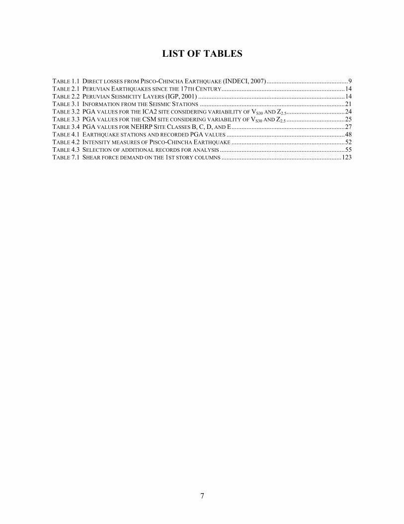
LIST OF TABLES TABLE 1.1 DIRECT LOSSES FROM PISCO-CHINCHA EARTHQUAKE (INDECI, 2007) ................................................. 9 TABLE 2.1 PERUVIAN EARTHQUAKES SINCE THE 17TH CENTURY .......................................................................... 14 TABLE 2.2 PERUVIAN SEISMICITY LAYERS (IGP, 2001) ........................................................................................ 14 TABLE 3.1 INFORMATION FROM THE SEISMIC STATIONS ....................................................................................... 21 TABLE 3.2 PGA VALUES FOR THE ICA2 SITE CONSIDERING VARIABILITY OF VS30 AND Z2.5 ................................... 24 TABLE 3.3 PGA VALUES FOR THE CSM SITE CONSIDERING VARIABILITY OF VS30 AND Z2.5 ................................... 25 TABLE 3.4 PGA VALUES FOR NEHRP SITE CLASSES B, C, D, AND E .................................................................... 27 TABLE 4.1 EARTHQUAKE STATIONS AND RECORDED PGA VALUES ....................................................................... 48 TABLE 4.2 INTENSITY MEASURES OF PISCO-CHINCHA EARTHQUAKE .................................................................... 52 TABLE 4.3 SELECTION OF ADDITIONAL RECORDS FOR ANALYSIS ........................................................................... 55 TABLE 7.1 SHEAR FORCE DEMAND ON THE 1ST STORY COLUMNS ........................................................................ 123

8
1 Overview
1.1 Macro-Seismic Data On August 15, 2007, at 6:40 p.m. local time (UTC/GMT: 11:40 p.m.), a strong offshore earthquake hit the coast of Central Peru. The epicenter was located 40 km WNW of the city of Chincha, 105 km NW of the city of Ica, and 150 km SSE of Lima, the capital of Peru (Figure 1.1). The coordinates of the epicenter are 13.354ºS, 76.509ºW according to the United States Geological Survey (USGS, 2008). The USGS estimated that the moment magnitude of this event was M=8.0 ± 0.1, and the hypocenter depth was between 26 km and 39 km.
Epicenter(13.32° S 76.51° W)
Lima (150 km)
ICA (115 km)
Pisco (51 km)
Chincha Alta(42 km)
50 km
100 km
150 km
Tambo de Mora (37 km)
Figure 1.1 Epicenter of the Pisco-Chincha Earthquake and affected cities
1.2 Damage and Casualties Data The cities of Pisco, Ica and Chincha Alta in the Ica Region were most affected, whilst the earthquake was also felt in the capital, Lima. Masonry structures are the most common single-family housing construction both in urban and rural areas of Peru in the last 45 years (Loaiza and Blondet, 2002). Masonry buildings in Peru consist of load bearing unreinforced masonry walls made of clay brick units, confined by cast-in-place reinforced concrete tie columns and beams. The majority of the deaths were caused by collapse of these masonry residential buildings. In addition, several masonry and adobe churches partially collapsed. In the seashore town closest to the epicenter, Tambo de Mora, many buildings were damaged due to differential settlement as a consequence of massive liquefaction of supporting soil. A highway

9
running from Lima to Pisco was damaged by landslides as well as lateral spreading. Facilities for utility networks, such as communication towers and electric poles, were damaged from both strong shaking and foundation failure. The Peruvian National Institute for Civil Defense (INDECI, 2007) reported that the death toll as of September 3, 2007 was 519 (Table 1.1). Close to 55,000 residential buildings collapsed and 21,000 were damaged. Many educational facilities and health centers were also adversely affected. Most of the deaths and damage were concentrated in the Ica region, which includes Chincha Alta, Pisco, and Ica. Among the total number of deaths from this earthquake, 66% were in Pisco. There were larger numbers of destroyed buildings in Chincha than Pisco, but the death toll was lower in Chincha as many buildings were damaged by liquefaction not by brittle collapse. Such a slow failure mode allowed residents to escape from buildings. In comparison with the number of damaged and destroyed residential masonry structures, engineered structures survived the earthquake relatively well, except for some reinforced concrete buildings. Damage to bridges was also not significant in number but substantial in terms of effect on transportation flow through the Pan-American Highway.
Table 1.1 Direct losses from Pisco-Chincha Earthquake (INDECI, 2007) People Housing Affected
bridges
Educational facility Health center
Injured Death Affected Destroyed Affected Destroyed Affected Destroyed
1,844 519 20,958 54,926 3 511 73 111 11
1.3 Field Mission Itinerary The MAE Center field reconnaissance team visited the most severely damaged areas in Peru. Peruvian researchers joined the MAE Center team and continued to contribute to the work after the mission. The MAE Center and Peruvian team spent six days in Peru for field work and for meetings with researchers in CISMID (Peru Japan Center for Seismological Investigations and Disaster Mitigation) and the Faculty of Civil Engineering at the National University of Engineering of Peru. The field mission details, composition of the team and areas of expertise are provided in Appendix A. Figure 1.2 shows the travel route of the team as recorded by the GPS travel log. Detailed GPS travel logs in each city are provided in Appendix A. The subsequent chapters of this report provide more detailed information on the performance of the built infrastructure and geotechnical observation of the earthquake.

10
Figure 1.2 GPS travel log of the entire site visit

11
2 Engineering Seismology
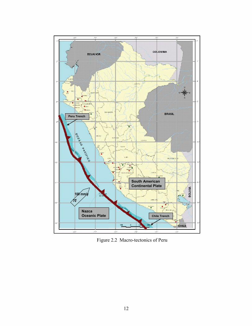
2.1 Local Geology and Tectonics The seismicity of Peru is dominated by the convergence of the Nazca oceanic plate and the western continental border of the South American plates (Barazangi and Isacks, 1976; Leffler et al., 1997). The components of plate subduction regions are depicted in Figure 2.1. The convergence of the two plates occurs by the subduction of the Nazca plate beneath the South American plate. An interesting feature of the regime is that the angle of dip is approximately 30 degrees in the southern segment, and changes to a much shallower, almost horizontal segment (<10 degrees) further north, thus tending towards an almost compressional regime (Tavera and Buforn, 2001). To accommodate the large difference in the dip angle, it is postulated that there is a major tear in the Nazca plate (Barazangi and Isacks, 1976). Further details of the layered seismicity are presented in Section 2.2. The subduction region is manifested in part by the offshore Peru-Chile trench. Figure 2.2 depicts the macro-tectonic setting of Peru. The main subduction mechanism has been associated with historical and contemporary earthquakes as discussed in the subsequent sections. The main mechanism of subduction results in high bending and friction stresses in the overriding South American plate that lead to seismicity observed inland in the Western Cordillera. The highly stressed subducting Nazca plate is also responsible for damaging earthquakes which are of shallow depth in the offshore and coastal segments. Both consequential intraplate mechanisms have resulted in significant seismic activity (Tavera et al., 2006).
Figure 2.1 Constituents of subduction regions are depicted
12
Figure 2.2 Macro-tectonics of Peru
NazcaOceanic Plate
South American Continental Plate
70- 100 mm/y
Peru Trench
Chile Trench
NazcaOceanic Plate
South American Continental Plate
70- 100 mm/y
Peru Trench
Chile Trench

13
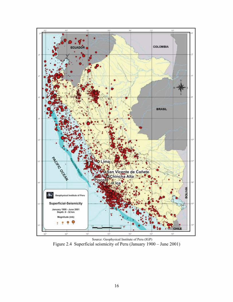
2.2 Brief History of Earthquakes in the Region A study of hypocenters of Peruvian earthquakes (Barazangi and Isacks, 1976) concluded that subduction of the Nazca plate beneath the South American plane fully explains the seismic activity in Peru. There are five segments of inclined seismic zones. The inclination in each zone is fairly uniform. The segment under northern and central Peru and that under central Chile have a very shallow dip of about 10o, whilst the segments under southern Ecuador, southern Peru and northern Chile have steeper dip angles of 20o-30o. There are interesting implications for this observation with regard to the distribution of earthquakes over depth in the subduction region. If the shallow dipping segments are in contact with the continental (South American) plate, then the thickness of the latter is less than 130 km, contrary to reports preceding Barazangi and Isacks (1976), where it was postulated that the South American plate is 300 km thick. In addition to seismic activity on the inclined subduction surfaces, there is considerable seismicity in the upper 50 km of the overriding plate. Finally, the aforementioned researchers report that there is a seismic gap between depths of 320 and 525 km. Table 2.1 lists the known earthquake activity in Peru and neighboring regions from the 17th century to the present time. Twenty-four damaging earthquakes were registered since 1900. Thus, it is speculated that there had been many unregistered earthquakes before 1900. The most deadly earthquake in Peru's history before 1900 struck Lima on October 1746. At least 5,000 people were killed, many of them when a seismic seawave (tsunami) swept the coast. On May 31, 1970 an earthquake and its aftershocks killed more than 66,000, and caused widespread landslides (USGS, 2007). As alluded to above, seismic activity on the Pacific Coast of South America is observed from the ground surface to a depth of about 700 km. Geophysical investigations have identified six layers of seismic activity (IGP, 2001) related to the energy released by earthquakes Table 2.2. The layers are: Superficial, for depths within 0-32 km; Intermediate-Superficial, 33-70 km; Intermediate, 71-150 km; Intermediate-Deep, 151-300 km; Mid-Deep, 301-540 km; and Deep, 541-667 km. According to several sources the Pisco-Chincha earthquake nucleated at a depth in the range between 26 and 39 km. This range falls in the boundary between the Superficial and Intermediate-Superficial seismicity layers +/- 6 km. The Superficial Seismicity zone comprises earthquakes at depths down to 32 km in a complex seismo-tectonic environment characterized by collision and re-accommodation events in the surface contact of the Nazca and South America plates, as described in Section 2.1. Almost 30% of the energy released by earthquakes in the period 1900-2001 was generated in this layer of seismicity. The Superficial-Intermediate Seismicity (SIS) zone of the Nazca fault system is characterized by a high concentration of earthquakes and consists of re-accommodation and subduction of seismic plates. The complex seismo-tectonic environment produces an elastic-plastic behavior of the crust material. This zone released about 43% of the earthquake-related energy in the period 1900-2001. The superficial and intermediate-superficial seismicity layers are important to understand the seismicity of Peru since over 70% of the energy released by all earthquakes and over 50% of the energy from major earthquakes (Mb>6) are released in these two zones. The Peruvian historical seismicity for earthquakes generated from all layers can be observed in Figure 2.3; the historical superficial and intermediate-superficial seismicity earthquake epicenters are shown in Figure 2.4 and Figure 2.5, respectively.

14
Table 2.1 Peruvian Earthquakes since the 17th Century Date Location Magnitude Fatalities
1619 02 14 Trujillo, Peru M 7.7 350 1664 05 12 Ica, Peru M 7.3 400 1687 10 20 Lima, Peru M 8.5 600 1746 10 28 Lima, Peru N/A 5,000 1821 07 10 Camana, Peru M 8.2 162 1868 08 13 Arica, Peru (now Chile) M 9.0 25,000 1908 12 12 Offshore Central Peru M 8.2 N/A 1913 11 04 Abancay, Peru N/A 150 1940 05 24 Callao, Peru M 8.2 249 1942 08 24 Offshore Central Peru M 8.2 30 1943 01 30 Yanaoca, Peru N/A 200 1946 11 10 Ancash, Peru M 7.3 1,400 1947 11 01 Satipo, Peru M 7.3 233 1948 05 11 Moquegua, Peru M 7.4 70 1950 05 21 Cusco, Peru M 6.0 83 1953 12 12 Tumbes, Peru M 7.4 7 1958 01 15 Arequipa, Peru M 7.3 28 1960 01 13 Arequipa, Peru M 7.5 57 1966 10 17 Near the Coast of Peru M 8.1 125 1968 06 19 Moyobamba, Peru M 6.9 46 1969 10 01 Comas region, Peru M 6.4 136 1970 05 31 Chimbote, Peru M 7.9 66,000 1974 10 03 Offshore Central Peru M 8.1 2001 06 23 Near the Coast of Peru M 8.4 138 2001 07 07 Near the Coast of Peru M 7.6 1 2002 10 12 Peru, Brazil border region M 6.9 2005 09 26 Northern Peru M 7.5 5 2006 10 20 Offshore Central Peru M 6.7 2007 08 15 Offshore Central Peru M 8.0 519 2007 11 16 Peru-Ecuador border M 6.8
Table 2.2 Peruvian Seismicity Layers (IGP, 2001)
Seismicity Depth (km)
% EQ % EQ (mb>6) Seismic Environment
Superficial 0-32 29.5 18.08 Collision and re-accommodation
Intermediate-Superficial 33-70 43.05 37.35 Re-accommodation and subduction
Intermediate 71-150 18.16 20.48 Subduction
Intermediate-Deep 151-300 8.93 8.43 Subduction
Mid-Deep 301-540 0.05 0.00 Subduction
Deep 541-667 0.31 15.66 Subduction

15
Source: Geophysical Institute of Peru (IGP)
Figure 2.3 Seismicity map (January 1900 – June 2001)
16
Source: Geophysical Institute of Peru (IGP)
Figure 2.4 Superficial seismicity of Peru (January 1900 – June 2001)

17
Source: Geophysical Institute of Peru (IGP)
Figure 2.5 Superficial intermediate seismicity for Peru (January 1900 – June 2001)

18
2.3 The Pisco-Chincha Earthquake
2.3.1 General Information and Rupture Models Several sources of information were consulted on the Pisco-Chincha earthquake. These are (i) the USGS report, which provides general information on the event; (ii) the teleseismic analysis reports posted by Konca, Vallée, and Yagi (all 2007), where three different rupture models were proposed and (iii) a comprehensive report published by the Geological Institute of Peru (IGP). Only a brief description of each document is presented hereafter. According to USGS, the earthquake hit on August 15th, 2007, at 6:40 p.m. local time (UTC/GMT: 11:40 p.m.), with an epicenter that is located 40 km WNW of Chincha City, 105 km NW of Ica City, and 150 km SSE of Lima City. The approximate coordinates of 13.354º S, 76.509º W were given. The estimated moment magnitude for this event was M=8.0, and the hypocenter depth H was 39 km. The model proposed by Konca (2007) is based on 18 P-wave and 19 SH-wave teleseismic records and indicates that the moment magnitude is also 8.0. The epicenter is given as 13.354º S, 76.509º W (adopted from the USGS report), and the hypocenter depth is 39 km. The rupture process is characterized by variable slip angle, an azimuth of the rupture plane of 324º, and a dip angle of 27º. The estimated rupture velocity is 1.5 km/s. The model of Vallée (2007) on the other hand, based on 15 P-wave teleseismic records, estimates moment magnitude of M=7.9, azimuth of 318º, dip angle of 20º, and variable slip angle. The source characterization consists of two rupture processes or zones of maximum displacement (asperities) separated by 60 seconds, with rupture velocity of 1.3 km/s. The third model summarized here is that of Yagi (2007), based on the analysis of 15 P-wave teleseismic records, proposes a moment magnitude of 8.1, azimuth of 320º, dip angle of 18º, and variable slip angle. The source model describes two rupture processes with total rupture duration of 180 seconds and average rupture velocity 1.75 km/sec. The Geophysical Institute of Peru reported that the Pisco-Chincha earthquake nucleated 74 km East of Pisco City with approximate epicenter coordinates 13.49ºS, 76.85ºW. The estimated hypocenter depth is 26 km. The fault plane solution proposed by Harvard and verified by the IGP (2001), shows an inverse mechanism with nodal planes almost horizontal and vertical; both oriented NNW-SSE (Figure 2.6). From the characteristics of the subduction process, the almost horizontal plane is the fault surface, which is characterized by an average dip angle of 14º. The Pisco-Chincha earthquake rupture process, located in the inter-plate contact surface of the Nazca and South American Plates, is complex and includes two ruptures; the second was stronger than the first. From an aftershock analysis undertaken by Tavera et al. (2007), three epicenter clouds where identified, referred to as G1, G2, and G3 in Figure 2.6. According to the authors, the aftershock distribution confirms the complexity of the rupture process. The arrow indicates the rupture propagation through the fault plane. The aftershock distribution delimits the fault plane proposed by the authors, which is consistent with the models of Vallée (2007) and Yagi (2007). The dimensions of the proposed fault rupture are 160 km x 125 km.

19
Figure 2.6 Fault plane solution and aftershock distribution
2.3.2 Comparison of Resulting Intensity with Previous Earthquakes The cities most affected by the earthquake were Pisco with an estimated Modified Mercalli Intensity (MMI) of VIII, followed by Chincha VII, Ica VI and Lima V. Old records of earthquakes affecting these cities describe impacts similar to those observed after the Pisco-Chincha earthquake. Extracts from reports on earthquakes in the 17th and 18th centuries are replicated below. In these events, the moment magnitude M was estimated employing macro-seismic data (IGP, 2001). On May 12, 1664, in Ica City, a 7.37 magnitude earthquake generated an intensity of X leaving 400 dead. The report describes the earthquake as follow: The ground was broken in many places. Water poured out of some wells of the city. Many huge tree roots were pulled out of the ground. On October 20, 1687, in Cañete City (Lima), a magnitude 9 earthquake with an intensity of IX left 100 casualties in Lima, 500 in Callao and surrounding places. The earthquake was described in an old report as follows: The noise was high. There were ‘Waves’ in the ground. Large cracks for many kilometers between Ica and Cañete. The city was very affected. A tidal wave destroyed the Pisco Port. On February 10, 1716, in Pisco City (Ica), an earthquake of magnitude 8.64 earthquake, with an intensity of IX, caused extensive damage in the city. Locals described the events as follows: The ground opened up; it ejected streams of dust and water with a terrible noise. All the houses were destroyed. The descriptions above are in line with the observations of the MAE Center reconnaissance mission and indicate that the effects of historical and contemporary earthquakes in Central Peru are rather similar.

20
3 Ground Motion Estimation in Central Peru
3.1 Ground Motion Models A ground motion model is a function that relates a ground intensity parameter (e.g. peak ground acceleration, velocity or displacement, spectral acceleration, velocity or displacement) with the distance between the seismic source (e.g. epicenter, fault line, fault plane, etc.) and the analysis site. In this report, the Pisco-Chincha earthquake scenario is analyzed using one of the most recent and comprehensive attenuation models, described below. It is noted and emphasized that the strong-ground motion model used hereafter is not for subduction regions. However, reliable subduction attenuation models are not available, and the earthquake source is complex enough to warrant a study based on the most recent and widely accepted attenuation model available. Reasonable assumptions are used to substitute for parameters that are either not available, or are specific to shallow crustal earthquakes for which the model was intended. A recent study on attenuation relationships for shallow crustal regions is the Next Generation Attenuation (NGA) Empirical Ground Motion Model, in which Campbell and Bozorgnia (2006) propose a trilinear quadratic functional form to estimate peak ground acceleration (PGA), peak ground velocity (PGV), peak ground displacement (PGD), and response spectral acceleration (SA) at periods ranging from 0.01 to 10.0 seconds. This model involves the following parameters: moment magnitude, closest distance to rupture, buried reverse faulting, normal faulting, sediment depth (both shallow and basin effects), hanging-wall effects, average shear-wave velocity in the top 30 m, and nonlinear soil response as a function of shear-wave velocity and rock PGA. Currently, the NGA model is believed to be the most comprehensive ad reliable because it includes parameters that are not considered in other proposals. Though this model was created to predict ground motion in the western USA, its use has been extended to other shallow crustal regions. An analysis carried out by Campbell and Bozorgnia (2006) and Stafford et al. (2008) show that the NGA-CB model can be used in Europe, for example. The MAE Center team has therefore decided to attempt a comparison between the model predictions and observed strong-motion from the current earthquake, in spite of the difference in source mechanisms. From reports on the 2007 earthquake, the seismic source parameters were defined (Section 3.3.1) to be employed in the attenuation analysis (Section 3.3.2), using reasonable assumptions where information was incomplete. The recorded PGA values from 13 stations (Section 3.3.1) were compared with the PGA values from the NGA-CB model (Section 3.3.3). The earthquake scenario defined in this section is further employed in the generation of the ground shaking maps presented in Section 3.4. 3.1.1 Information from Seismic Stations In order to compare the attenuation model results with recorded peak ground acceleration values, an extensive search of ground motion information for the Pisco-Chincha earthquake was carried out. Peak ground acceleration values for 13 stations managed by four organizations (IGP, CISMID, SEDAPAL, and PUCP) were collected and shown in Table 3.1.

21
Table 3.1 Information from the Seismic Stations Station Code
Station Name Organization Location Latitude Longitude Elevation PGA (g)
(º South) (º West) AMSL (m) NS EW
ANC ANCON IGP Ancón Observatory - IGP, Lima 11.5900 76.1500 46 0.056 0.060
CAL CAL-CISMID CISMID DHN, Callao 12.0600 77.1500 36 0.103 0.098
CIP CIP-CISMID CISMID San Isidro, Lima 12.0920 77.0490 NA 0.060 0.056
CSM CSM-CISMID CISMID CISMD-FIC-UNI, Lima 12.0133 77.0502 130 0.046 0.075
EST1 ESTANQUE-1 SEDAPAL Lima 12.0330 76.9750 279 0.051 0.056
EST2 ESTANQUE-2 SEDAPAL Lima 12.0350 76.9720 276 0.013 0.021
ICA2 UNSLG CISMID Ica, Ica 14.0887 75.7321 409 0.341 0.278
LMO LA MOLINA IGP UNA, La Molina, Lima 12.0850 76.9480 260 0.022 0.026
MAY MAYORAZGO IGP IGP, Mayorazgo, Lima 12.0550 76.9440 315 0.061 0.056
MOL LA MOLINA CISMID La Molina, Lima 12.1000 76.8900 145 0.070 0.080
NNA ÑAÑA IGP ÑAÑA, Lima 11.9870 76.8390 575 0.019 0.023
PAR PARCONA IGP Parcona Locality, Ica 14.0420 75.6990 555 0.464 0.498
PUCP U. CATOLICA PUCP Lima 12.0706 77.0798 NA 0.061 0.068
Acronyms
IGP: Geophysical Institute of Peru
CISMID: Peruvian-Japanese Center for Earthquake Engineering and Disaster Mitigation, Faculty of Civil Engineering (FIC) of the National University of Engineering (UNI)
UNA: National Agricultural University, La Molina, Peru
DHN: Directorate of Hydrography and Navigation - Peru
3.1.2 Estimation of Peak Ground Acceleration with the NGA-CB Model The expression for the estimation of PGA by the NGA model comprises six parameters that represent the effects of: magnitude ( magf ), distance to the seismic source ( disf ), fault type ( fltf ), hanging walls ( hngf ), shallow site response ( sitef ), and deep site response ( sedf ). ln mag dis flt hng site sedPGA f f f f f f (3.1)
Magnitude term, fmag, depends only on the magnitude of the event; for magnitudes higher than 6.5, it can be computed with Eq. (3.2), where the constants C0, C1, C2, and C3 have values -1.715, 0.5, -0.53, and -0.262, respectively. The magnitude used for the Pisco-Chincha earthquake attenuation analysis is M=8.0 (USGS, 2007). However, considering the reports summarized in Section 3.3.1, M could range between 7.9 and 8.1. For the generation of the PGA maps shown in Section 3.3.3, fmag is equal to 0.567.
0 1 2 3( 5.5) ( 6.5)magf C C M C M C M (3.2)
The distance term, disf , depends of the moment magnitude M and the closest distance to the coseismic rupture plane, RUPR , in km, Eq. (3.3). The constants 4C , 5C , and 6C have values -2.118, 0.17, and 5.6, respectively. The parameter disf was computed for each point of the grid used for the generation of the ground motion maps shown in Section 3.3.3.

22
2 24 5 6lndis RUPf C C M R C (3.3)
In the NGA-CB model, the faulty type term, fltf , is the variable that represents the fault type, Eq. (3.4). For the case of the Pisco-Chincha earthquake: 0NMF since it was not a normal faulting process. Therefore the second term of the right side of Eq. (3.4) is zero. Since the earthquake is a reverse faulting event, 1.0RVF . The constants 7C and 8C , have values 0.28 and -0.12, respectively. The parameter ,flt Zf is a term that depends of the depth to the top of the coseismic rupture plane TORZ : if 1TORZ , ,flt Z TORf Z ; and if 1TORZ , , 1flt Zf . TORZ is a seismic parameter that is not explicitly defined in the earthquake fault model (Tavera et al., 2007b); however, an additional analysis (shown below) indicates that TORZ could range between 4 and 5 km. Therefore in this case, , 1flt Zf and 7 0.28fltf C .
7 , 8flt RV flt Z NMf C F f C F (3.4)
TORZ is the depth to the top of the coseismic rupture plane. Considering that the subduction fault plane (Tavera et al., 2007b) has a constant dip angle 14º and the extension of the subduction plane maintains the same angle searching the surface in the Peru-Chile trench, the estimated average value for TORZ is 4.45 km.
Figure 3.1 Fault plane – profile view
The NGA model considers that the hanging-wall effect depends of four parameters, Eq. (3.5): fhng,R, which is in terms of the distances to the rupture plane – RUPR and JBR –; ,hng Mf , a magnitude-dependent term; ,hng Zf , which depends of the already defined parameter TORZ ; and
,hngf , a factor that depends of the dip angle . In Eq. (3.5), 9 0.49C .
9 , , , ,hng hng R hng M hng Z hngf C f f f f (3.5)
The definition of the four factors of Eq. (3.5) for the case of the Pisco-Chincha earthquake is described as follow. ,hng Rf is defined by Eq. (3.6), being JBR the closest distance to the surface projection of the coseismic rupture plane (in km). The second part of Eq. (3.6) is only valid for 1TORZ . , 1hng Mf since 6.5M ; and , 1hngf since 70 . ,hng Zf , defined by Eq. (3.7) and valid only for 0 20TORZ , is equal to 0.778.

23
,
1 0
0JB
hng RRUP JB RUP JB
Rf
R R R R
(3.6)
, 20 / 20hng Z TORf Z (3.7)
The shallow site response term, sitef , depends on the average shear-wave velocity in the top 30 m of the site profile 30SV (m/s) and the value of PGA with 30 1100 m/sSV 1110A . The constants 10C , 2k , c , and n , have values 1.058, -1.186, 1.88, and 1.18, respectively. For the computation of the ground shaking maps (Section 3.3.3), the 30SV values used in the analyses are 150, 255, 525, and 1070 m/s, which correspond to the NEHRP site classes B, C, D, and E, respectively. Since there is no information of 1110A for the large region covered by the ground shaking maps, the method employed in this report to estimate this parameter is that suggested by the authors of the NGA formulations (Campbell and Bozorgnia, 2007). It consists of the estimation of 1110A using sitef for 110030 SV in Eq (3.1).
30 3010 2 1110 1110 30
3010 2 30
3010 2 30
ln ln ln 865865 865
ln 865 1100865
ln 11001110
n
S SS
Ssite S
SS
V VC k A c A c V
Vf C k n V
VC k n V
(3.8)
The deep site response term, sedf , depends of the depth to the 2.5 km/s shear-wave velocity horizon (sediment depth) 2.5Z , in km, according to Eq. (3.9). The constants 11C , 12C , and 3k , have values 0.04, 0.61, and 1.839, respectively. Since 2.5Z is unknown for the large extent of the ground shaking maps of Section 3.3.3, those maps where computed with 2.5 2.0Z , a default value suggested by Campbell and Bozorgnia (2007). In other words, those maps do not include the effects of sediment depth in the ground shaking estimation. In order to investigate the impact of other values of 2.5Z , a sensitivity analysis for sites located in Lima and Ica is presented below.
2.5
11 2.5 2.5
2.5
0.25 30.7512 3 2.5
1 1
0 1 3
1 3
sed
Z
C Z Z
f Z
C k e e Z
(3.9)
The estimation of 30SV and 2.5Z requires the assessment of shear-wave velocity profiles for the sites of interest. Central Peru is vast and maps of those parameters are not available. In order to address this lack of information, a sensitivity analysis is presented to study the impact of the variability of 30SV and 2.5Z on PGA. Two locations, Lima and Ica Cities were chosen for the analysis. For Ica City, the location of the ICA2 Station was taken as a reference site.

24
For the case of Lima City, the chosen station was CSM. The range of values for 30SV is 150 to 1070 m/s, and for 2.5Z the range is 0.5 to 4.5 km. 3.1.2.1 Sensitivity Analysis for Ica City (ICA2 Station Site) For the sensitivity analysis in Ica City the distances JBR and RUPR are necessary. The source mechanism employed in the attenuation analysis (Figure 3.1) shows that Ica City is over the seismic fault plane, which indicates that 0 kmJBR . In other hand, the shortest distance from ICA2 station to the fault plane is 31.36 kmRUPR . In the NGA model, variations in 30SV and 2.5Z (Table 3.2 and Figure 3.2) do not give a constant patter of variation for the site classes. For instance, for Site Class E ( 30 150 m/sSV and 2.50.5 4.5 kmZ ), PGA shows two peaks at 2.5 1 kmZ ( 0.494 gPGA ) and
2.5 3.5 kmZ ( 0.479 gPGA ). For Site Classes B, C and E, peaks at those 2.5Z values (1 and 3.5 km) are not observed. Another case is for 2.5 0.5 kmZ and 30150 1070 m/sSV , a peak is observed for 30 180 m/sSV ( 0.445 gPGA ). For the other Site Classes (i.e., B, D, and E) there are no peaks at the value of 30 180 m/sSV .
Table 3.2 PGA values for the ICA2 site considering variability of VS30 and Z2.5 NEHRP Site
Class VS30 (m/s)
Z2.5 (km)
0.5 1 1.5 – 3 3.5 4 4.5
B 1070 0.226 0.230 0.230 0.245 0.259 0.272 BC 760 0.254 0.259 0.259 0.274 0.288 0.301 C 525 0.291 0.294 0.294 0.303 0.313 0.322
CD 360 0.335 0.334 0.334 0.333 0.333 0.335 D 255 0.384 0.376 0.376 0.356 0.344 0.337
DE 180 0.445 0.423 0.423 0.373 0.344 0.325 E 150 0.230 0.494 0.451 0.479 0.400 0.355

25
Figure 3.2 Variability of PGA with respect to VS30 and Z2.5 for Ica
3.1.2.2 Sensitivity Analysis for Lima (ICA2 Station Site)
The sensitivity analysis developed for Lima followed the same procedure used for Ica. The distances to the fault plane, employed in the attenuation analysis, are Rjb = 123.63 km and RRUP = 128.39 km. By analyzing the results from the sensitivity analysis (Table 3.3 and Figure 3.3), it is concluded that similar trends exist between the two cases studied in terms of variation of PGA. On the other hand, the PGA values for Lima are much lower than for Ica.
Table 3.3 PGA values for the CSM site considering variability of VS30 and Z2.5 NEHRP
Site Class VS30 (m/s)
Z2.5 (km) 0.5 1 1.5 – 3 3.5 4 4.5
B 1070 0.054 0.055 0.055 0.059 0.062 0.065 BC 760 0.061 0.062 0.062 0.066 0.069 0.072 C 525 0.070 0.071 0.071 0.073 0.075 0.077
CD 360 0.081 0.080 0.080 0.080 0.080 0.081 D 255 0.092 0.090 0.090 0.086 0.083 0.081
DE 180 0.107 0.102 0.102 0.090 0.083 0.078 E 150 0.086 0.119 0.108 0.115 0.096 0.086

26
Figure 3.3 Variability of PGA with respect to VS30 and Z2.5 for Lima City
3.1.3 Comparison of Computed and Recorded PGA Values Following the procedure described in Section 3.3.2, the PGA values for the available 13 stations were computed, for 30SV values corresponding to the site classes B, C, D, and E
(Table 3.4). The epistemic uncertainty in the estimation of PGA was computed with a model proposed by the USGS for use in the 2007 update of the National Seismic Hazard Maps (NSHMP, 2007), which is described by Eq. (3.10). ln PGA is an incremental value of median PGA intended to represent approximately one standard deviation ( ) of the epistemic
probability ground motion distribution. The values recommended for ln PGA (Campbell and Bozorgnia, 2007) for events with moment magnitude 7.0M with the characteristics
10 kmRUPR , ln 0.4PGA ; for 10 30 kmRUPR , ln 0.36PGA ; and for 30 kmRUPR , ln 0.31PGA . In Table 3.4, PGA and PGA represent the lower and upper bounds
of the PGA estimation accounting for the epistemic uncertainty.
ln ln lnuncPGA PGA PGA (3.10)

27
Table 3.4 PGA values for NEHRP Site Classes B, C, D, and E
Station PGA
(Station) NEHRP* A1110 (g)
NEHRP Site Classes
E (VS30=150 m/s) D (VS30=255 m/s) C (VS30=525 m/s) B (VS30=1070 m/s)
PGA -
PGA PGA +
PGA-
PGA PGA+
PGA-
PGA PGA +
PGA -
PGA PGA+
ANC 0.060 C 0.046 0.056 0.076 0.104 0.051 0.070 0.095 0.043 0.058 0.079 0.034 0.047 0.064
CAL 0.103 E 0.054 0.064 0.087 0.119 0.059 0.081 0.110 0.050 0.068 0.093 0.040 0.055 0.075
CIP 0.060 B 0.057 0.067 0.091 0.124 0.062 0.085 0.116 0.053 0.072 0.098 0.043 0.058 0.079
CSM 0.075 C, D 0.055 0.064 0.088 0.120 0.060 0.082 0.111 0.050 0.069 0.094 0.041 0.055 0.076
EST1 0.056 B 0.057 0.066 0.090 0.123 0.062 0.084 0.115 0.052 0.071 0.097 0.042 0.058 0.078
EST2 0.021 - 0.057 0.066 0.091 0.123 0.062 0.084 0.115 0.052 0.071 0.097 0.042 0.058 0.079
ICA2 0.341 C, D 0.228 0.170 0.232 0.317 0.193 0.264 0.359 0.195 0.266 0.363 0.169 0.230 0.314
LMO 0.026 - 0.059 0.068 0.093 0.127 0.064 0.087 0.119 0.054 0.074 0.101 0.044 0.060 0.082
MAY 0.061 B 0.058 0.068 0.092 0.126 0.063 0.086 0.117 0.054 0.073 0.100 0.043 0.059 0.080
MOL 0.080 C 0.061 0.070 0.096 0.130 0.066 0.090 0.122 0.056 0.076 0.104 0.045 0.062 0.084
NNA 0.023 - 0.058 0.067 0.091 0.124 0.062 0.085 0.116 0.053 0.072 0.098 0.043 0.058 0.079
PAR 0.498 C, D 0.221 0.168 0.228 0.311 0.189 0.257 0.351 0.190 0.258 0.352 0.164 0.223 0.304
PUCP 0.068 C 0.056 0.065 0.089 0.122 0.061 0.083 0.113 0.052 0.070 0.096 0.042 0.057 0.077
* NEHRP site class with the closest PGA mean value to the recorded PGA (station). The computed PGA values are based on a scenario with Z2.5=2.0 km; other Z2.5 values produce different results.
In Table 3.4, NEHRP* indicates the site class, defined according to the NEHRP provisions (BSSC, 2004). It is important to mention that sediment effects are not included in the analysis since the value employed for the estimation of PGA is 2.5 2.0 kmZ . If the site sediment layers are associated with 2.5Z values lower than 1.0 km or higher than 3.0 km, NEHRP* could not point towards an appropriate site class. Comments are given in the station-by-station analysis with regard to site class, and the availability or otherwise of information on site soil condition. 3.1.3.1 Ground Motion Analysis for Stations EST2, LMO, and NNA
EST2, LMO, and NNA stations recorded very low PGA values in comparison to other stations located in Lima City. The recorded PGA values of 0.021g for EST2, 0.026g for LMO, and 0.023g for NNA, are far from the estimated ground motion for rock sites, represented through the parameter A1110, which is the lowest possible PGA from the NGA. In Figure 3.4, it is observed that the NGA model predicts higher PGA values (A1110) for the mentioned stations; i.e., 0.058g for EST2, 0.06g for LMO, and 0.058g for NNA. The difference between the recorded and estimated PGA values confirms one of the features of the NGA model, as stated by the authors. The prediction of ground motion for very hard soils (e.g. NEHRP site class A) is inaccurate. Bernal and Tavera (2007b) state that these stations, EST2, LMO, and NNA, recorded very low PGA values since they are located on very hard rock sites at the hills

28
of Lima City in the Localities of Santa Anita (EST2 station), La Molina (LMO station), and Ñaña (NNA).
Figure 3.4 Map of estimated PGA for rock sites (NGA-CB parameter A1110)
3.1.3.2 Ground Motion Analysis for Stations CIP, EST1, and MAY
The comparison between the recorded PGA values at stations CIP (0.06g), EST1 (0.056g), and MAY (0.061g), and the mean PGA values obtained from the NGA attenuation analysis; Table 3.4 shows that, ignoring sediment effects (e.g. 2.5 2.0 kmZ ), those stations could be
located on sites with NEHRP class B (Figure 3.5). However, according to Bernal and Tavera (2007b), those stations are not located on rock (site class B), but rather on alluvial gravel soils (stations CIP and EST1), and sand-lime soils (station MAY). It is important to note that the site class analysis described above does not consider the epistemic uncertainty in the PGA

29
estimation. It is possible that the site class for stations CIP, EST1 and MAY is C; for the three cases, the recorded PGA value falls in the upper and lower PGA bounds indicated in Table 3.4. For station CIP, the recorded PGA value of 0.06g falls in the range 0.053g to 0.098g (site class C); for station EST1, 0.056g falls in the range 0.052g-0.097g; and for station MAY, 0.061g falls in the range 0.054g-0.1g. Another plausible explanation for the low PGA values in the stations investigated above could be the effect of smaller depth sediment layers (Z2.5 < 1.0 km), which could slightly reduce the estimated PGA value. For instance, for CIP station, the mean PGA value for site class C is 0.072g for Z2.5 < 2.0 km. However, for Z2.5 < 0.2 km, the PGA value for the same site class is reduced to 0.0697g.
Figure 3.5 PGA map for Site Class B (VS30=1070 m/s)

30
3.1.3.3 Ground Motion Analysis for Station ANC
The predicted mean PGA value for site class C is 0.058g, for the ANC station (Figure 3.6), is very close to the recorded PGA value at that station (0.06g). According to Bernal and Tavera (2007b), this station is located on alluvial gravel soils, which could be characterized by site classes C, D, or E, depending on the 30SV values for this site. Additional site analyses are required to determine which site class better represents the location of this recording station.
Figure 3.6 PGA map for Site Class C (VS30=525 m/s)

31
3.1.3.4 Ground Motion Analysis for Stations CSM, MOL, and PUCP
The stations CSM, MOL, and PUCP are located in the Districts of Rimac, La Molina, and San Miguel in Lima, respectively. The stations PUCP and CSM are located on alluvial gravel soils, and the MOL station is on sand-lime soils. During the Pisco-Chincha earthquake, the recorded PGA values for those stations were: for CSM, 0.075g; for MOL, 0.08g; and for PUCP, 0.068g. The analytically-predicted PGA values for site class C are closer to the recorded PGA values in those stations (Table 3.4 and Figure 3.6). For the case of the CSM station, the PGA values for site class D are equally close to the recorded PGA value than the values for the site class C. The predicted site class could be either C or D (Figure 3.6 and Figure 3.7). Site specific analyses are required to better classify the sites where the mentioned stations are located. The predicted values are however reasonable.
Figure 3.7 PGA map for Site Class D (VS30=255 m/s)

32
3.1.3.5 Ground Motion Analysis for Stations ICA2 and PAR
From the set of 13 seismic stations, the ICA2 and PAR stations recorded the highest PGA values. ICA2 station, located at the southern part of Ica, lays on silty-sand soils (Bernal and Tavera, 2007a). ICA2 recorded a PGA value of 0.341g, a value much higher than those recorded at the Lima stations. From the attenuation analysis, the estimated NEHRP* site classes (Table 3.4), which mean PGA value are closer to the recorded PGA value, are C and D (Figure 3.7). The recorded value in ICA2 of 0.341g falls into the range for site class C (0.195g-0.363g), and for site class D (0.193g-0.359g). In the PAR station, the recorded PGA value of 0.498g falls out of the ranges for site classes C and D possibly due to the amplification caused by the superficial layer of lime-sand soil (Bernal and Tavera, 2007a). Further work, which is beyond the scope of this report, is required to definitively determine the site class.
Figure 3.8 PGA map for Site Class E (VS30=150 m/s)

33
3.1.3.6 Ground Motion Analysis for Stations CAL
The PGA value recorded at the CAL station of 0.103 g is the highest PGA value recorded in Lima. The particular soft soil layers, characterized by very low shear wave velocities, between 40-120 m/s (Bernal and Tavera, 2007b), amplified ground motion. The NEHRP* site class for CAL station is E (Figure 3.8), which seems consistent with the characteristics of the soils at the station site. The recorded PGA falls in the range of PGAs for site class E (0.064g-0.119g) and for site class D (0.059g-0.11g).
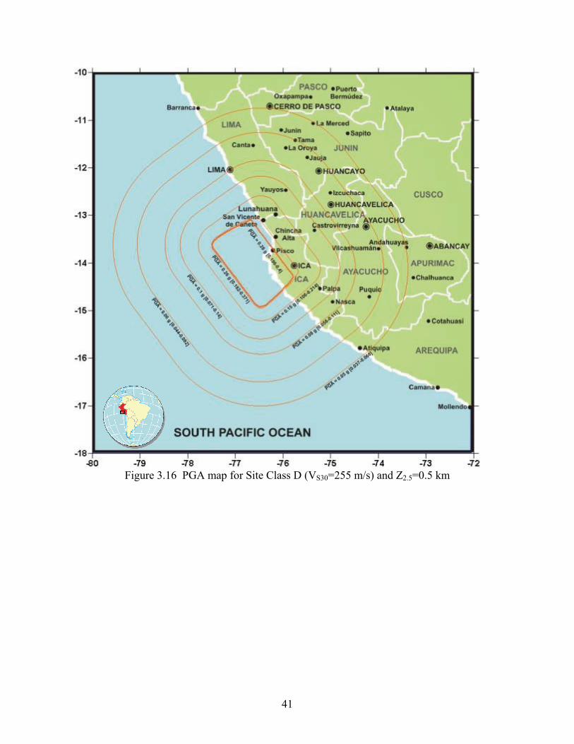
3.2 Ground Motion Maps for Central Peru The above brief study of the applicability of the NGA strong-motion model, which was developed with no subduction records, to the Pisco-Chincha earthquake indicates that reasonable agreement exists between predictions and observations in most cases. It may therefore be of interest to generate ground motion maps for this earthquake that are useful for engineering purposes. For the computation of such ground motion maps a coordinate grid (81x81 points and cell size of 11,1 x 11,1 km²), for latitudes between -72º and -80º, and longitudes between -10º and 18º, was used to compute PGA employing Eq. (3.1) to (3.9). For the generation of the contour lines an interpolation method type point Kriging was used (Isaaks and Srivastava, 1989).
The NGA ground motion parameter – A1110 – was computed for Central Peru by using Eq. (3.8), for VS30 = 1100 m/s, and Eq. (3.1). The A1110 map (Figure 3.9) shows the predicted PGA values on rock and is used for the computation of the ground motion maps for NEHRP site classes B to E, shown in Figure 3.5 to Figure 3.21. The estimated A1110 values for important cities can be obtained from Figure 3.9. By computing the PGAs for NEHRP site classes B to E, and for three sediment depths Z2.5= 0.5, 2.5, and 3.5 km (Figure 3.10 to Figure 3.21), it is observed that major changes in PGA are found for site classes B and C, for VS30 values of 255 and 150 m/s, respectively. In general, the lower the VS30, the higher is the variability in PGA. The same tendency is observed in the sensitivity analysis for Ica and Lima (Figure 3.2).

34
Figure 3.9 Map for rock (VS30=1110 m/s) – NGA-CB Variable A1110

35
Figure 3.10 PGA map for Site Class B (VS30=1070 m/s) and Z2.5=0.5 km

36
Figure 3.11 PGA map for Site Class B (VS30=1070 m/s) and Z2.5=2.0 km

37
Figure 3.12 PGA map for Site Class B (VS30=1070 m/s) and Z2.5=3.5 km

38
Figure 3.13 PGA map for Site Class C (VS30=525 m/s) and Z2.5=0.5 km

39
Figure 3.14 PGA map for Site Class C (VS30=525 m/s) and Z2.5=2.0 km

40
Figure 3.15 PGA map for Site Class C (VS30=525 m/s) and Z2.5=3.5 km
41
Figure 3.16 PGA map for Site Class D (VS30=255 m/s) and Z2.5=0.5 km

42
Figure 3.17 PGA map for Site Class D (VS30=255 m/s) and Z2.5=2.0 km

43
Figure 3.18 PGA map for Site Class D (VS30=255 m/s) and Z2.5=3.5 km

44
Figure 3.19 PGA map for Site Class E (VS30=150 m/s) and Z2.5=0.5 km

45
Figure 3.20 PGA map for Site Class E (VS30=150 m/s) and Z2.5=2.0 km

46
Figure 3.21 PGA map for Site Class E (VS30=150 m/s) and Z2.5=3.5 km

47
3.3 Discussion and Conclusions The main objective of Chapter 3 is to present plausible ground motion maps for Central Peru based on the characteristics of the 2007 Pisco-Chincha earthquake. Towards this objective, the most recent, comprehensive and accepted ground motion attenuation model proposed by Campbell and Bozorgnia (2007) is employed, notwithstanding that the relationships are not intended for subduction regimes. Fault plane solutions for the Nazca and South-America subduction regime, based on technical reports of the Pisco-Chincha earthquake, were used in making assumptions suitable for the use of the selected ground motion model. Due to the lack of shear-wave velocity profile information for the 13 seismic stations, for which peak ground accelerations were available, two of the NGA parameters could not be directly evaluated for the attenuation analysis. These two parameters are 30SV , the average shear-wave velocity in the top 30 m of the site profile, and 2.5Z , the depth to the 2.5 km/s shear-wave velocity horizon (sediment depth). In order to address the lack of information on these parameters, PGA prediction sensitivity analyses for two sites located in Lima and Ica were undertaken. The PGA estimation showed higher variability in soft soils than in hard soils, as expected. For example, it was observed that for 30SV values lower than 255 m/s (site classes D and E), PGA varies significantly for 2.50.5 4.5 kmZ . Comparison between predictions and observations shows that good agreement exists in many cases, and the observations are within the range of variability obtained from the predictive equations. In other cases, assumptions were necessary with regard to the soil class, in addition to the site characterization parameters mentioned above. Further site specific studies are required if better constrained values of peak ground parameters are to be obtained from the attenuation models. On the whole, the investigation presented in this chapter indicate that the NGA strong-motion model results in reasonable estimates of ground motion, even though it was not derived for subduction mechanisms. The ground motion maps for Central Peru proposed in this report can be used to estimate peak ground accelerations in important sites (e.g. towns and major cities) in Central Peru for the Pisco-Chincha earthquake. More reliable estimates of the ground shaking due to this earthquake would be obtained if the same exercise presented above is repeated after deriving accurate soil characterization maps for the region. Moreover, the uncertainty in the model, alluded to above, should also be taken into account when selecting design PGAs. Apart from the significant assumption of using a non-subduction attenuation model to evaluate strong-ground motion associated with a subduction region, another limitation was the NGA constraint for ground motion at very hard soils (NEHRP site class A). As a consequence, the recorded PGA values at three hard-rock stations, all of them located in Lima, could not be reliably compared with estimated PGA values.

48
4 Strong-motion Data Analysis
4.1 Strong-motion Stations and Records The Pisco-Chincha earthquake was recorded by several stations in Peru, as described above. Emphasis is placed in this chapter on the time series, as opposed to the peak ground parameters addressed in Section 3. The organizations operating seismographs are listed at the bottom of Table 4.1. A total of 16 ground motion stations in Peru recorded the earthquake. During and after field investigations, recorded ground motions from nine stations were obtained. The remaining records were not released to the MAE Center reconnaissance team. Table 4.1 lists the earthquake stations where ground motions were recorded. Most stations were located in Lima and Ica. The PGA values in Lima vary from 0.013g to 0.117g with an average of 0.057g. A maximum PGA of 0.50g was recorded at PAR station in Ica with an epicentral distance of 116 km. Most available ground motions were not baseline corrected. Before processing ground motions for response spectra, baselines were corrected with linear polynomials implemented in the ground motion processing software SeismoSignal Ver 3.2.0.
Table 4.1 Earthquake stations and recorded PGA values Station code
Station name Location LAT, S LON,
W Epicentral Dist., km
Organization PGA, CM/SEC2
V N E
EST2 Estanque-2 Lima 12.035 76.972 155 Sedapal 11.76 12.74 20.58
LMO La Molina Lima 12.085 76.948 149 IGP 14.18 21.17 25.31
NNA ÑAÑA Lima 11.987 76.839 156 IGP 21.60 18.70 22.10
ANC Ancon Lima 11.590 76.150 200 IGP 27.80 54.70 58.40
EST1 Estanque-1 Lima 12.033 76.975 155 Sedapal 30.38 49.98 54.88
MAY Mayorazgo Lima 12.055 76.944 152 IGP 31.22 59.77 55.00
CAL Hidrografía Callao 12.060 77.150 160 CISMID 31.63 101.00 95.76
CSM Jorge Alva-
Hurtado Lima 12.013 77.050 160 CISMID 32.90 45.10 73.90
CIP San Isidro Lima 12.090 77.049 152 CISMID 33.05 58.77 54.66
CER Ceresis Lima N/A N/A N/A Ceresis,
IGP 37.36 57.96 58.67
PUCP U. Catolica Lima 12.073 77.079 155 Ceresis 39.69 59.58 67.03
MOL La Molina Lima 12.100 76.890 145 CISMID 57.09 69.05 78.73
RIN Rinconada Lima N/A N/A N/A Ceresis,
IGP 57.72 115.20 111.37
ANR Asamblea Nac. De Rectores Lima N/A N/A N/A
Ceresis, IGP
73.53 65.38 85.26
ICA2 UNSLG Ica 14.089 75.732 117 CISMID 192.20 334.10 272.20
PAR Parcona Ica 14.042 75.699 116 IGP 301.10 455.00 488.00
Note CERESIS: Seismological Regional Center for South America SEDAPAL: Lima Water Company IGP: Geophysical Institute of Peru CISMID: Peruvian-Japanese Center for Earthquake Engineering and Disaster Mitigation of the National University of Engineering of Peru
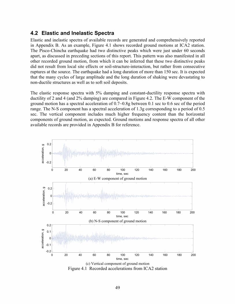
49
4.2 Elastic and Inelastic Spectra Elastic and inelastic spectra of available records are generated and comprehensively reported in Appendix B. As an example, Figure 4.1 shows recorded ground motions at ICA2 station. The Pisco-Chincha earthquake had two distinctive peaks which were just under 60 seconds apart, as discussed in preceding sections of this report. This pattern was also manifested in all other recorded ground motion, from which it can be inferred that these two distinctive peaks did not result from local site effects or soil-structure-interaction, but rather from consecutive ruptures at the source. The earthquake had a long duration of more than 150 sec. It is expected that the many cycles of large amplitude and the long duration of shaking were devastating to non-ductile structures as well as to soft soil deposits. The elastic response spectra with 5% damping and constant-ductility response spectra with ductility of 2 and 4 (and 2% damping) are compared in Figure 4.2. The E-W component of the ground motion has a spectral acceleration of 0.7~0.8g between 0.1 sec to 0.6 sec of the period range. The N-S component has a spectral acceleration of 1.3g corresponding to a period of 0.5 sec. The vertical component includes much higher frequency content than the horizontal components of ground motion, as expected. Ground motions and response spectra of all other available records are provided in Appendix B for reference.
0 20 40 60 80 100 120 140 160 180 200
-0.2
0
0.2
time, sec
acce
lera
tion,
g
(a) E-W component of ground motion
0 20 40 60 80 100 120 140 160 180 200
-0.2
0
0.2
time, sec
acce
lera
tion,
g
(b) N-S component of ground motion
0 20 40 60 80 100 120 140 160 180 200-0.2
-0.1
0
0.1
0.2
time, sec
acce
lera
tion,
g
(c) Vertical component of ground motion
Figure 4.1 Recorded accelerations from ICA2 station

50
0 0.5 1 1.5 2 2.5 30
0.5
1
1.5
Period, sec
Spe
ctra
l acc
eler
atio
n, g
Elastic, =5%
Ductility=2, =2%
Ductility=4, =2%
(a) Elastic and inelastic spectra of E-W component
0 0.5 1 1.5 2 2.5 30
0.5
1
1.5
Period, sec
Spe
ctra
l acc
eler
atio
n, g
Elastic, =5%
Ductility=2, =2%
Ductility=4, =2%
(b) Elastic and inelastic spectra of N-S component
0 0.5 1 1.5 2 2.5 30
0.5
1
1.5
Period, sec
Spe
ctra
l acc
eler
atio
n, g
Elastic, =5%
Ductility=2, =2%
Ductility=4, =2%
(c) Elastic and inelastic spectra of vertical component
Figure 4.2 Response spectrum of recorded accelerations at ICA2 station

51
4.3 Energy Flux and Intensity Measures Various parameters may be used to characterize recorded ground motion. Peak values in the time domain, such as PGA, PGV, and PGD, are the most frequently used parameters to define the intensity of ground motions. But these values miss many other important features of ground motion. Inelastic response of structures can be affected by ground motion parameters such as frequency content, duration, number of large amplitude cycles, energy flux, amongst others. This section presents some important intensity measures which characterize the recorded ground motions and allude to their potential to cause damage. It is noted that the method adopted for baseline correction significantly affects the velocity and the displacement time-histories. Hence, the following parameters may not be directly comparable to the parameters of ground motions processed with a different baseline correction method.
Peak ground acceleration, max | ( ) |PGA a t (4.1) Peak ground velocity, max | ( ) |PGV v t (4.2) Peak ground displacement, max | ( ) |PGD d t (4.3)
Root-mean-square of acceleration, 2
0
1( )
rt
rmsr
a a t dtt
(4.4)
Root-mean-square of velocity, 2
0
1( )
rt
rmsr
v v t dtt
(4.5)
Root-mean-square of displacement, 2
0
1( )
rt
rmsr
d d t dtt
(4.6)
Peak velocity-acceleration ratio, max max/ /v a PGV PGA (4.7)
Arias intensity, 2
0( )
2aI a t dtg
(4.8)
Specific energy density, 2
0( )
rtSED v t dt (4.9)
where ( )a t , ( )v t , ( )d t , and rt are recorded acceleration, velocity, displacement, and total
duration of record, respectively. The evaluated intensity measures are presented in Table 4.2. As a reference, the parameters of other earthquake ground motions from comparable previous damaging earthquakes are also presented. For comparison with the largest record from the Pisco-Chincha Earthquake (ICA2 station with PGA of 0.341g) earthquake stations which recorded ground motions with PGA of around 0.3g from other earthquakes are selected. Figure 4.3 compares energy flux of the Pisco-Chincha Earthquake with other events. Due to the prolonged ground motion duration, it is clear that the Pisco-Chincha record has a much larger energy flux than other earthquake records with similar PGA levels.

52
Table 4.2 Intensity measures of Pisco-Chincha Earthquake
Earthquake Station Comp. PGA, gPGV,
cm/secPGD, cm
Vmax
/Amax, sec
RMS Acc, g
RMS Vel,
cm/sec
RMS Disp, cm
Ia m/sec
SED, m2/sec
Pisco-Chincha, 2007
ANR
L 0.067 5.72 8.25 0.088 0.013 1.061 4.91 0.400 184
T 0.087 9.21 10.46 0.108 0.014 1.284 5.62 0.465 270
V 0.075 6.41 24.86 0.087 0.010 1.000 12.81 0.238 164
CAL
E 0.103 13.28 9.60 0.132 0.012 1.736 3.57 0.570 753
N 0.098 11.44 18.44 0.120 0.013 1.782 10.43 0.598 794
V 0.032 4.76 7.12 0.151 0.005 0.750 1.29 0.095 141
CER
L 0.059 5.81 7.86 0.100 0.010 1.026 2.52 0.235 173
T 0.060 7.69 29.22 0.131 0.010 1.254 14.12 0.234 259
V 0.038 4.99 18.76 0.134 0.007 0.953 8.70 0.121 149
CIP
E 0.056 9.49 8.56 0.174 0.007 0.932 4.25 0.180 217
N 0.060 4.82 6.84 0.082 0.006 0.644 2.48 0.148 104
V 0.034 4.59 6.69 0.139 0.005 0.664 2.52 0.078 110
CSM
E 0.075 7.38 9.10 0.100 0.009 0.725 3.45 0.331 131
N 0.048 3.26 6.21 0.070 0.008 0.510 2.43 0.215 65
V 0.034 3.80 9.16 0.116 0.005 0.554 4.74 0.079 77
ICA2
E 0.278 39.30 48.97 0.144 0.030 5.375 27.12 3.041 6300
N 0.341 63.57 33.19 0.190 0.033 7.743 9.30 3.698 13074
V 0.196 15.68 22.50 0.082 0.021 2.720 11.18 1.500 1613
MOL
E 0.080 6.28 7.47 0.080 0.011 0.722 2.09 0.440 130
N 0.070 4.10 4.54 0.059 0.010 0.535 1.63 0.365 71
V 0.058 3.40 6.01 0.060 0.008 0.547 1.52 0.250 75
PUCP
L 0.069 8.60 19.50 0.128 0.009 1.310 12.04 0.227 291
T 0.061 5.00 20.52 0.084 0.009 1.041 13.18 0.201 184
V 0.059 3.91 33.77 0.068 0.008 0.656 17.62 0.270 108
RIN
L 0.117 4.74 23.41 0.041 0.015 0.758 11.72 0.834 144
T 0.114 7.26 12.38 0.065 0.016 0.957 4.63 1.009 229
V 0.059 3.91 33.77 0.068 0.008 0.656 17.62 0.270 108
LomaPrieta, 1989 Gilroy Array #2 0 0.367 32.90 7.18 0.091 0.044 4.679 1.46 1.197 875
Northridge, 1994 Beverly Hills V 0.327 16.82 2.56 0.053 0.054 3.722 0.64 1.349 415
Kobe, 1995 Kakogawa 90 0.345 27.65 9.60 0.082 0.052 6.299 2.28 1.687 1625
Kocaeli, 1999 Duzce 180 0.312 58.83 44.09 0.192 0.051 16.433 15.46 1.085 7339

53
0
2000
4000
6000
8000
10000
12000
14000
0 20 40 60 80 100 120 140time, sec
Sp
ec
ific
En
erg
y D
en
sit
y,
cm
2/s
ec
Loma Prieta, 1989
Northridge, 1994
Kocaeli, 1999
Kobe, 1995
Pisco-Chincha, 2007
Figure 4.3 Energy flux of Pisco-Chincha earthquake in comparison with other events
4.4 Selection of Additional Records for Analysis It is essential for engineers to have a suite of ground motions to evaluate structural performance for a particular earthquake. Even though the Pisco-Chincha earthquake was recorded at several strong-motion stations as in Table 4.1, there are few records (probably one single record) of engineering usefulness that have been released for general use. The epicentral distance of the strong motion stations ranged from 116 km to 200 km. Most of the stations are located in Lima, too far from the source to generate useful records. To augment the recorded ground motions, a suite of ground motions recorded from during other earthquakes are selected. The ground motions are carefully chosen with the following criteria:
Fits a well-established attenuation model that shows reasonable correlation with the recorded motion
Recorded on stiff-to-rock soil condition Generated by earthquakes of moment magnitude of 4.0 or higher
Whereas Chapter 3 utilizes the NGA relationship, it was decided here to use the widely used attenuation model of Ambraseys et al. (2005a and 2005b). Figure 4.4 compares the PGA of horizontal acceleration of selected ground motions with the selected attenuation model. Figure 4.5 compares the vertical component of the acceleration. The selected ground motions and corresponding earthquake events and ground motion stations are summarized in Table 4.3. This suite of ground motion acceleration records is recommended for use in back-analysis of the performance of structures in the Pisco-Chincha earthquake, if the need arises.
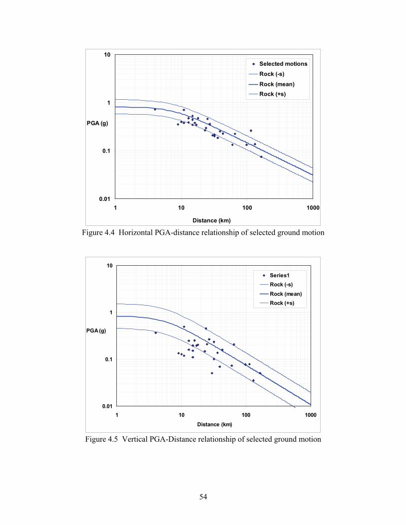
54
0.01
0.1
1
10
1 10 100 1000
Distance (km)
PGA (g)
Selected motions
Rock (-s)
Rock (mean)
Rock (+s)
Figure 4.4 Horizontal PGA-distance relationship of selected ground motion
0.01
0.1
1
10
1 10 100 1000
Distance (km)
PGA (g)
Series1
Rock (-s)
Rock (mean)
Rock (+s)
Figure 4.5 Vertical PGA-Distance relationship of selected ground motion

55
Tab
le 4
.3 S
elec
tion
of
addi
tion
al r
ecor
ds f
or a
naly
sis
Ear
thq
uak
e
Dat
e a
nd
Tim
e (U
TC
)S
tati
on
S
oil
con
dit
ion
Ep
ic.
D
ist.
[km
]P
GA
, H
. [g
]P
GA
, H
. [g
]P
GA
, V
. [g
]
afte
rsho
ck o
f Fri
uli e
arth
quak
e,Ita
ly
9/15
/197
63:
15:1
9B
RE
(B
regi
nj-F
abr
ika
IGLI
,Slo
ven
ia)
stiff
soi
l 18
0.
474
0.50
50.
204
afte
rsho
ck o
f Fri
uli e
arth
quak
e,Ita
ly
9/15
/197
69:
21:1
9F
OG
(F
org
aria
-Cor
nio,
Italy
)
stiff
soi
l 17
0.
346
0.33
60.
196
afte
rsho
ck o
f Mo
nten
egro
ear
thq
uak
e,Y
ugos
lavi
a 5/
24/1
979
17:2
3:18
BA
R (
Bar
-Sku
pstin
a O
pstin
e,Y
ugo
slav
ia)
st
iff s
oil
32
0.20
20.
270
0.10
1
afte
rsho
ck o
f Ra
cha
eart
hqua
ke,G
eorg
ia
5/3/
1991
20:1
9:39
SA
MB
(A
mbr
ola
uri,G
eorg
ia)
so
ft so
il 9
0.35
20.
509
0.13
6
afte
rsho
ck o
f Um
bro-
Ma
rchi
gian
a ea
rthq
uake
,Ital
y 4/
3/19
987:
26:0
0N
CR
(N
ocer
a U
mbr
a,Ita
ly)
rock
10
0.
398
0.28
20.
127
afte
rsho
ck o
f Um
bro-
Ma
rchi
gian
a ea
rthq
uake
,Ital
y 10
/6/1
997
23:2
4:00
NC
R (
Noc
era
Um
bra,
Italy
)
rock
11
0.
377
0.30
90.
119
afte
rsho
ck o
f Um
bro-
Ma
rchi
gian
a ea
rthq
uake
,Ital
y 10
/11/
1997
3:20
:56
NC
R (
Noc
era
Um
bra,
Italy
)
rock
15
0.
438
0.35
40.
196
afte
rsho
ck o
f Um
bro-
Ma
rchi
gian
a ea
rthq
uake
,Ital
y
10/1
6/19
9712
:00:
31C
LC (
Col
fiorit
o-C
aser
met
te,It
aly)
so
ft so
il 4
0.71
30.
385
0.36
5
Arp
iola
,Ital
y
3/22
/198
40:
16:2
4T
RG
(T
regn
ago,
Ital
y)
rock
16
4 0.
074
0.12
20.
051
Ath
ens,
Gre
ece
9/
7/19
9911
:56:
50A
TH
3 (A
then
s 3
(Kal
lithe
a D
istr
ict)
,Gre
ece)
ro
ck
23
0.26
50.
307
0.14
8
Cam
pano
Luc
ano,
Italy
11
/23/
1980
18:3
4:52
BR
N (
Brie
nza,
Italy
)
st
iff s
oil
43
0.22
70.
174
0.15
9
Cam
pano
Luc
ano,
Italy
11
/23/
1980
18:3
4:52
ST
R (
Stu
rno,
Italy
)
rock
32
0.
216
0.32
30.
235
Den
izli,
Tur
key
8/
19/1
976
1:12
:40
DN
Z (
Den
izli-
Bay
indi
rlik
ve Is
kan
Mud
urlu
gu,T
urke
y)st
iff s
oil
15
0.34
50.
261
0.15
4
Erz
inca
n,T
urke
y 3/
13/1
992
17:1
8:40
ER
C (
Erz
inca
n-M
eteo
rolo
gij M
udur
lugu
,Tu
rke
y)
stiff
soi
l 13
0.
389
0.51
30.
248
Friu
li,Ita
ly
5/
6/19
7620
:00:
13T
LM1
(Tol
mez
zo-D
iga
Am
bies
ta,It
aly)
ro
ck
27
0.35
70.
316
0.26
7
Ioni
an,G
reec
e
11
/4/1
973
15:5
2:12
LEF
(Le
fkad
a-O
TE
Bui
ldin
g,G
ree
ce)
soft
soil
15
0.52
50.
255
0.11
2
Koc
aeli,
Tur
key
8/17
/199
90:
01:4
0A
TS
(A
mba
rli-T
erm
ik S
antr
ali,T
urke
y)
rock
11
4 0.
263
0.17
60.
079
Lazi
o A
bruz
zo,It
aly
5/7/
1984
17:4
9:43
SC
F (
Sca
fa,It
aly)
ro
ck
60
0.13
20.
126
0.07
4
Man
jil,Ir
an
6/20
/199
021
:00:
08A
BH
(A
bhar
,Ira
n)
so
ft so
il 98
0.
132
0.20
90.
077
Man
jil,Ir
an
6/20
/199
021
:00:
08T
ON
(T
one
kabu
n,Ir
an)
so
ft so
il 13
1 0.
137
0.08
90.
036
Mon
tene
gro,
Yug
osla
via
4/
15/1
979
6:19
:41
BA
R (
Bar
-Sku
pstin
a O
pstin
e,Y
ugo
slav
ia)
st
iff s
oil
16
0.37
50.
363
0.25
3
Mon
tene
gro,
Yug
osla
via
4/
15/1
979
6:19
:41
HR
Z (
Her
ceg
No
vi-O
.S. D
. Pav
icic
,Yug
osla
via)
ro
ck
65
0.22
40.
256
0.20
9
Mon
tene
gro,
Yug
osla
via
4/
15/1
979
6:19
:41
PE
TO
(P
etro
vac-
Hot
el O
liva,
Yug
osl
avia
)
stiff
soi
l 25
0.
454
0.30
60.
213
Mon
tene
gro,
Yug
osla
via
4/
15/1
979
6:19
:41
ULO
(U
lcin
j-Hot
el O
limpi
c,Y
ugos
lavi
a)
stiff
soi
l 24
0.
294
0.24
10.
458
Sic
ilia-
Orie
ntal
e,It
aly
12
/13/
1990
0:24
:48
CA
T (
Cat
ania
-Pia
na,It
aly)
soft
soil
39
0.25
30.
182
0.07
0
Spi
tak,
Arm
enia
12
/7/1
988
7:41
:24
GU
K (
Guk
asia
n,A
rmen
ia)
so
ft so
il 36
0.
183
0.18
30.
138
Um
bria
,Ital
y
4/29
/198
45:
02:5
9N
CR
(N
ocer
a U
mbr
a,Ita
ly)
ro
ck
30
0.20
90.
160
0.05
1
Um
bro-
Mar
chig
iano
,Ital
y 9/
26/1
997
0:33
:16
NC
R (
Noc
era
Um
bra,
Italy
)
rock
13
0.
470
0.34
90.
162
Um
bro-
Mar
chig
iano
,Ital
y
9/26
/199
79:
40:3
0N
CR
(N
ocer
a U
mbr
a,Ita
ly)
ro
ck
11
0.71
20.
760
0.49
9

56
5 Geotechnical Aspects
5.1 Geology and Site Conditions
5.1.1 Geology of Cañete, Jahuay, Chincha and Tambo de Mora The zone of San Vicente de Cañete is located on an alluvial deposit of the recent Quaternary, flanked on the north and south by elevations that conform to part of the Cañete Formation of the Pleistocene and the Paracas Formation of the Tertiary Period of the Eocene. At the north part of Cañete City, in the zone of San Luis, some monzodiorite outcrops that belong to the batholithic of the coast can be observed. In Jahuay Beach, which is located between San Vicente de Cañete and Chincha, two predominant formations can be observed from Punta Iguana to La Perla Beach. These formations are the Cañete Formation that can be observed at the left side of the road and marine deposits at the right side of the road going southward from Lima City.
5.1.1.1 The Cañete Formation
This is a continental-origin formation composed by old alluvial accumulations derived from alluvial cones that have formed consolidated polimitic conglomerates of rounded to sub-rounded gravels, with lenticular intercalation of sand with varied granulometry, which can show crossed stratigrafy. The described litology changes southward because in the coast cliffs in Northern Jahuay an intercalation of sandy and lime conglomerates, along with sediments, can be observed. By contrast, in the cliffs of the Jahuay area and the Topará ravine the sequence is basically constituted by fine to coarse grayish sand, in sub-horizontal layers with thickness from 20 cm to 2 m with several pebble beds. Clay-lime lenses of 30 cm to 1 m are also intercalated. Toward the end of the sequence some yellowish cream lime clayish layers can be found, alternating with fine to coarse sand in continuous and lensy layers. Some of the layers have cross stratification where the layer thickness is estimated between 90 and 100 m.
5.1.1.2 Sea Deposits On numerous beaches at the seaboard of the study area can be found small, stepped terraces that can reach heights of 8 m above the mean sea level. These are covered inland by alluvial deposits, or are related to scarps. Chincha City is located on alluvial deposits (Qr-al) that consist of river accumulations of loose materials or poorly consolidated materials of heterogeneous and heterometric nature, conformed by blocks, pebbles and sub-rounded gravels, covered by a sand-slime matrix deposited during the Holocene. In the Chincha area has been identified sedimentary, igneous and metamorphic rocks, which range in age from the Jurassic-Cretaceous to the Recent Quaternary. A formation that can be distinguished in close zones to the city is the Topará Formation, belonging to the Quaternary-Pleistocene.

57
5.1.1.3 The Topará Formation
The outcrops of this formation are situated on the beachfront from the Topará ravine to the localities of Chincha Alta. Lithologically, this formation consist of thin clay layers with intercalations of friable sandstone with almost-horizontal crossed stratigrafy. The deposits of the Topará Formation have originated residual clay-sandy soils, with variable depth and permeability. The geology of Tambo de Mora City is defined by deposits of the recent Quaternary conformed by alluvial deposits. North of Tambo de Mora, the Formation Cañete can be seen, and in the south are the terraces produced by the Chico River. They run from the heights, crossing hills like the Mirador and Bolsa, which are monzogranitic outcrops from the batholithic of the coast. 5.1.2 Geology of the Huamani Bridge, Pisco, Paracas and Ica In these zones can be seen stratigraphic units that belong to the Cenozoic age of the Recent Quaternary, formed by sea deposits, alluvial, eluvial and eolic. Additionally, in surrounding zones, stratigraphic units from the Upper Tertiary represented by the Formation Pisco and the Lower Tertiary represented by the Formation Paracas, are observed.
5.1.2.1 The Pisco Formation
This formation is described as a white lithological sequence comprised by diatomites, with intercalations of sandstone tuffs and lutite, which flourishes from the Pisco River to the surrounding communities of Camaná. The study area is exposed from Caucato Hill, from the north of the bridge on the Pisco River to the southern limit of the Ica quadrangle. This unit flourishes as the shape of a layer that gets wider southward, where it occupies almost all the width of the Ica quadrangle. In the right riverside of the Pisco River, a 500-meter-width section of white diatomites appears; this sequence apparently belongs to The Cañete Formation. In this sector, the Pisco Formation sections show a marked monotony consisting primarily of very pure white diatomites that appear tuff-like and intercalate with thin layers of grayish white sandy tuffs.
5.1.2.2 Alluvial and Eluvial Deposits These kinds of deposits consist of the clastic deposits transported by water and accumulated mainly in the ravines or from the Andine foothills. These deposits form the wide alluvial plain terrains typical of the coastal plains. The accumulated deposits in the ravine bottoms, composed of thick conglomerates intercalated with sand, lime and clay, are well exposed in the cut of the rivers and at the terrace feet. In the tributary ravines, where the drainage is cyclic, and sometimes undertaken in a violent way, the deposits are constituted by the material carried, which is primarily represented by mudstones that contain rock fragments of several sizes.

58
5.1.2.3 Eolian Materials
In the seashore of the study area some deposits accumulated by wind are widely distributed. The oldest ones form an extensive, thin sand coat that is not wider than 1.0 m in the most cumulated areas. Sands are composed of coarse grains with a dark gray color due to its high content of ferromagnesians. These deposits generally display a wavy surface, like ripple marks. The finest white sand coats, composed of a majority of quartz, show a great mobility and are distributed widely in invading dark sand zones.
5.1.2.4 Sea Deposits In the seacoast of the study area some early sea quaternary deposits are exposed. Their distribution is mainly restrained to zones located in the internal ends of the bays that are not favorable for the accumulation of materials.

59
Figure 5.1 Geology of Cañete and Chincha (Ingemmet, 1994)

60
Figure 5.2 Geology of Pisco and Paracas (Ingemmet, 1994)

61
5.2 Damage to Foundations It was observed that in some zones foundations and structures were severely affected due to ground settlement and liquefaction, which caused the reduction of soil bearing capacity and lateral displacement. The greatest foundation damage was observed in the Tambo de Mora District, where some houses collapsed due to soil liquefaction. This District is located in the Province of Chincha on alluvial and sea deposits. The water table in the zone is high (0.5 to 1.0 m), reaching in some places the ground level, as it is observed in Figure 5.3. A large amount of damage was observed on Alfonso Ugarte Street. There, the houses suffered settlements up to 0.90 m and the rise of the internal floors due to the ejection of water and sand originated by soil liquefaction. In this zone, large cracks were observed, and were extended on houses and roads. Local residents declared that in some cases the water ejection reached more than 1.0 m above ground level.
a) Settlement of 1.0 m in a house b) Rise of internal floors caused by the ejection of
water and sand
c) Cracks and settlement in a house
d) Settlement of houses. Detail of the water table level
after the earthquake. Figure 5.3 House damage caused by the settlement of foundations. Alfonso Ugarte Street in
Tambo de Mora District
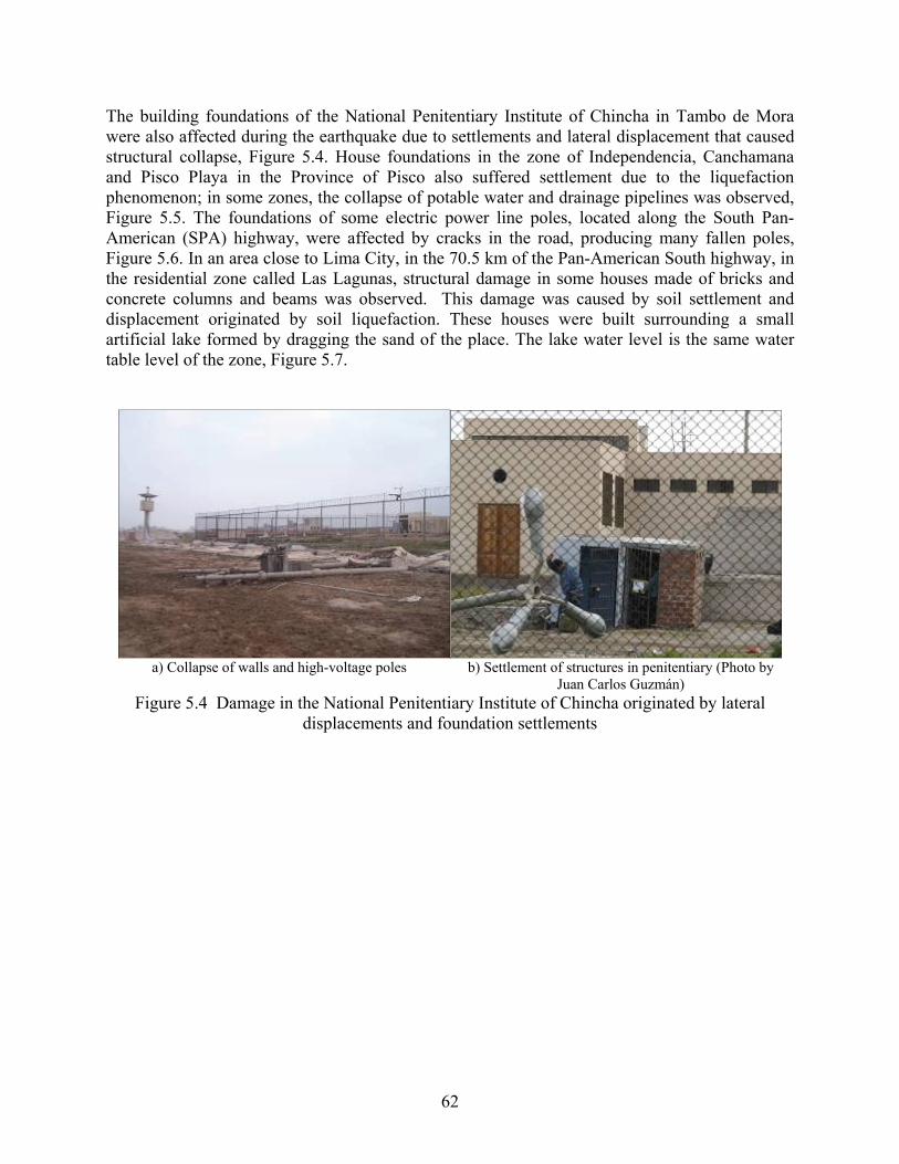
62
The building foundations of the National Penitentiary Institute of Chincha in Tambo de Mora were also affected during the earthquake due to settlements and lateral displacement that caused structural collapse, Figure 5.4. House foundations in the zone of Independencia, Canchamana and Pisco Playa in the Province of Pisco also suffered settlement due to the liquefaction phenomenon; in some zones, the collapse of potable water and drainage pipelines was observed, Figure 5.5. The foundations of some electric power line poles, located along the South Pan-American (SPA) highway, were affected by cracks in the road, producing many fallen poles, Figure 5.6. In an area close to Lima City, in the 70.5 km of the Pan-American South highway, in the residential zone called Las Lagunas, structural damage in some houses made of bricks and concrete columns and beams was observed. This damage was caused by soil settlement and displacement originated by soil liquefaction. These houses were built surrounding a small artificial lake formed by dragging the sand of the place. The lake water level is the same water table level of the zone, Figure 5.7.
a) Collapse of walls and high-voltage poles
b) Settlement of structures in penitentiary (Photo by
Juan Carlos Guzmán) Figure 5.4 Damage in the National Penitentiary Institute of Chincha originated by lateral
displacements and foundation settlements

63
a) Structural settlement in Pisco Playa
b) Leaning electricity poles in Pisco Playa
c) Damage in Malecón Miranda
d) Settlements and damage in the drainage were
observed in San Juan de Dios Street. Figure 5.5 Damage in structure foundations in Pisco
a) Fall of poles in the 78 km of the South Pan-
American Highway b) Fall of poles in the 218 km caused by liquefaction
Figure 5.6 Toppling of poles along the Pan-American Highway caused by ground failures
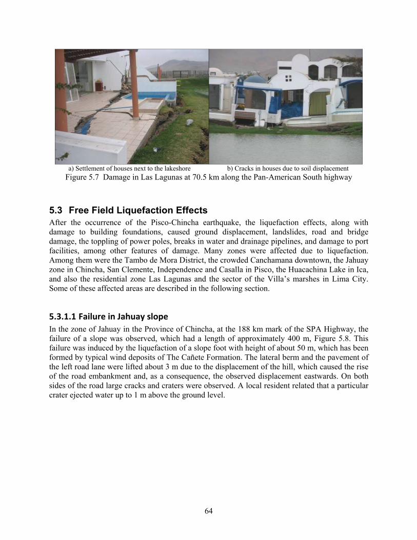
64
a) Settlement of houses next to the lakeshore b) Cracks in houses due to soil displacement
Figure 5.7 Damage in Las Lagunas at 70.5 km along the Pan-American South highway
5.3 Free Field Liquefaction Effects After the occurrence of the Pisco-Chincha earthquake, the liquefaction effects, along with damage to building foundations, caused ground displacement, landslides, road and bridge damage, the toppling of power poles, breaks in water and drainage pipelines, and damage to port facilities, among other features of damage. Many zones were affected due to liquefaction. Among them were the Tambo de Mora District, the crowded Canchamana downtown, the Jahuay zone in Chincha, San Clemente, Independence and Casalla in Pisco, the Huacachina Lake in Ica, and also the residential zone Las Lagunas and the sector of the Villa’s marshes in Lima City. Some of these affected areas are described in the following section.
5.3.1.1 Failure in Jahuay slope In the zone of Jahuay in the Province of Chincha, at the 188 km mark of the SPA Highway, the failure of a slope was observed, which had a length of approximately 400 m, Figure 5.8. This failure was induced by the liquefaction of a slope foot with height of about 50 m, which has been formed by typical wind deposits of The Cañete Formation. The lateral berm and the pavement of the left road lane were lifted about 3 m due to the displacement of the hill, which caused the rise of the road embankment and, as a consequence, the observed displacement eastwards. On both sides of the road large cracks and craters were observed. A local resident related that a particular crater ejected water up to 1 m above the ground level.

65
a) Embankment displacement of about 400 m b) Lifting of berm and left lane of road
c) Displacement of road eastward d) Cracks produced in the zone
Figure 5.8 Soil displacement in the Jahuay in the 188 km of the SPA Highway caused by liquefaction in the slope foot
5.3.1.2 Lateral Ground Displacement in Canchamana
In the crowded Canchamana downtown, located 2.5 km northward from Tambo de Mora in Chincha, some cases of massive lateral ground displacement were observed, caused by the liquefaction of the seacoast terrace, Figure 5.9. The displaced area presumably has a width of 1.0 km and length of more than 3.0 km. In a local road, between Canchamana and Victoria, a maximum vertical displacement of 3.0 m was observed. In the same zone, ground cracks were observed parallel to the seacoast with widths of up to 1.0 m; in some cracks evidence of water and sand ejection was clear, Figure 5.10. Due to the extension of the lateral displacements in the zone of Canchamana, caused by soil liquefaction, the 8-meter-height embankment of the 91 km SPA Highway suffered settlements, affecting concrete sewers located in the zone, Figure 5.11. Evidence of water and sand ejections as well as cracks close to the embankment base were found.

66
a) Soil cracks due to lateral displacement b) Large vertical displacement in the affected zone
Figure 5.9 Lateral ground displacement due to soil liquefaction
a) Settlement in the left road lane b) Evidence of ejection of water and sand close to the
embankment base Figure 5.10 Damage at the 191 km mark of the S PA Highway due to lateral displacement
a) View of a concrete sewer under the embankment b) Damage in a sewer due to lateral displacement
Figure 5.11 Damage in sewer due to lateral displacement
3.0 m
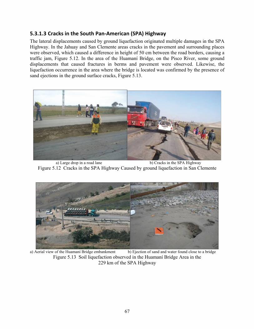
67
5.3.1.3 Cracks in the South Pan‐American (SPA) Highway
The lateral displacements caused by ground liquefaction originated multiple damages in the SPA Highway. In the Jahuay and San Clemente areas cracks in the pavement and surrounding places were observed, which caused a difference in height of 50 cm between the road borders, causing a traffic jam, Figure 5.12. In the area of the Huamaní Bridge, on the Pisco River, some ground displacements that caused fractures in berms and pavement were observed. Likewise, the liquefaction occurrence in the area where the bridge is located was confirmed by the presence of sand ejections in the ground surface cracks, Figure 5.13.
a) Large drop in a road lane b) Cracks in the SPA Highway
Figure 5.12 Cracks in the SPA Highway Caused by ground liquefaction in San Clemente
a) Aerial view of the Huamaní Bridge embankment b) Ejection of sand and water found close to a bridge
Figure 5.13 Soil liquefaction observed in the Huamaní Bridge Area in the 229 km of the SPA Highway

68
5.3.1.4 Damage in San Martín Port
San Martín Port, which is located in Punta Pejerrey, Paracas, was affected by ground liquefaction. This was evidenced with lateral displacements that caused cracks with widths of about 25 cm, the formation of sand volcanoes, and vertical displacement of about 80 cm. The most affected places were those where the port facilities are located, in areas near to the sea.
a) Structural collapse due to ground cracks in areas
gained to the sea b) Vertical displacement of 80
cm Figure 5.14 Damage in the San Martín Port caused by liquefaction
5.3.1.5 Damage in Lima City
Close to Lima City, in the zone of Los Pantanos de Villa in Chorrillos District, cracks that caused leaning in poles and ground settlement were observed.
a) Ground displacement due to soil liquefaction b) Cracks in the pavement and berm of the highway
Figure 5.15 Cracks in Defensores del Morro Avenue in Los Pantanos de Villa

69
6 Structural Engineering Aspects
6.1 Regional Damage Description and Statistics
6.1.1 Pisco Pisco is a seashore city located 51 km in the south east direction from the epicenter. The death toll in Pisco was 338, which represents 65% of the total casualties from the Pisco-Chincha earthquake. A large number of residential buildings were damaged (6,022) or collapsed (10,131). The damage to the city mostly resulted from collapse of masonry structures due to prolonged strong ground shaking. Ground motions in Pisco were not recorded, as earthquake stations were not available in the city. From the hazard analysis in Chapter 3, it is expected that the city may have suffered earthquake ground motion with PGA of about 0.25g, with an exceptionally long duration of 120-150 seconds. Flood marks from a tsunami wave were observed during the field investigation. No evidence of widespread liquefaction was recorded. Site characteristics of Pisco were thoroughly studied prior to the Pisco-Chincha Earthquake by Peruvian researchers, as alluded to in Chapter 5 above. Based on many geotechnical tests and borehole data, the city was divided into four zones (Figure 6.1). The site investigation team visited parts of Zone III and Zone IV in Figure 6.1. From the widespread of earthquake damage in the city, it was anticipated that Zone I and II also suffered similar damage to that presented in the following sub-sections.
Figure 6.1 Micro-zonation of Pisco (Murrugarra et al., 1999)

70
The majority of residential buildings were made of adobe reinforced with natural fibers (thin wood splinters), plain masonry structure with cement bricks, masonry structure with RC confinement, or occasionally RC frame structure. Most of the masonry or adobe structures have either collapsed or were heavily damaged. Many reinforced concrete structures were also damaged. Some of the RC structures were remarkably intact. In the following, representative pictures of damaged structures are presented with brief comments. The locations of the place where the pictures are taken are given in Figure 6.2. Masonry structures are not covered in the report.
Fig 6.13, 5.14Fig 6.4
Fig 6.25
Fig 6.26
Fig 6.21, 5.23Fig 6.22
Fig 6.24 Fig 6.20
Fig 6.17, 5.18
Fig 6.15, 5.16
Fig 6.9
Fig 6.8
Fig 6.7
Fig 6.6
Fig 6.3
Figure 6.2 Locations of structures in Figure 6.3 to 6.26

71
6.1.1.1 Adobe Structures The majority of damaged and collapsed structures were made of adobe or masonry. Several residential structures were built in two stories with adobe. When adobe is used, natural fibers, such as thin wooden sticks, are used to reinforce adobe wall, Figure 6.6.
Figure 6.3 Residential building made of reinforced adobe-1
Figure 6.4 Residential building made of reinforced adobe-2
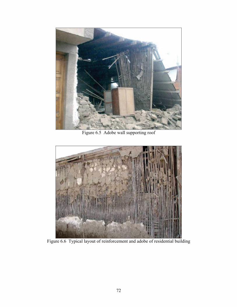
72
Figure 6.5 Adobe wall supporting roof
Figure 6.6 Typical layout of reinforcement and adobe of residential building

73
6.1.1.2 Masonry Structures
Masonry was used for both residential and many of non-residential buildings. Non-residential buildings, Figure 6.7 and Figure 6.8, were typically constructed with thick masonry walls. Even in these buildings no or very little reinforcements were used. Figure 6.12 shows a building which had soft 1st story. Both 1st and 2nd stories were built with masonry without reinforcement.
Figure 6.7 Collapsed masonry structure-1
Figure 6.8 Collapsed masonry structure-2
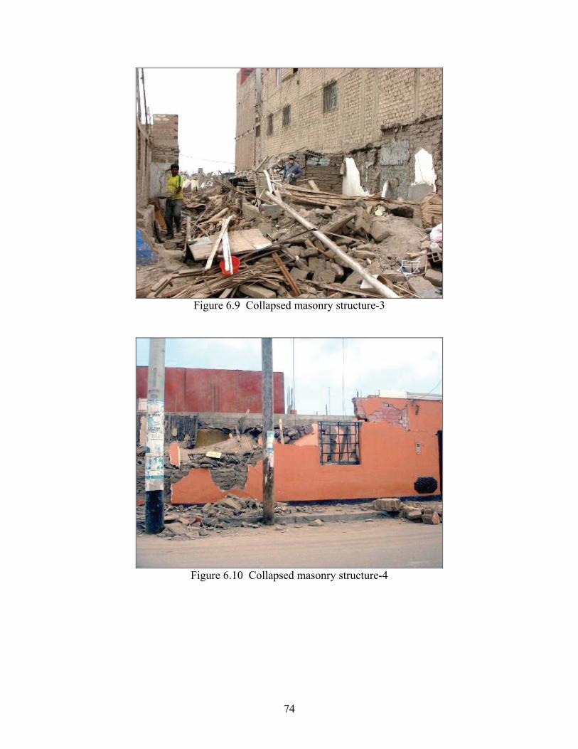
74
Figure 6.9 Collapsed masonry structure-3
Figure 6.10 Collapsed masonry structure-4

75
Figure 6.11 Collapsed masonry structure-5
Figure 6.12 Collapsed masonry structure with RC columns-6

76
6.1.1.3 Reinforced Concrete Structures In Figure 6.13, the first story was used as a parking lot. In comparison with the massive second and third stories, first story was very weak. This picture shows the typical failure mode of a building with soft story. Figure 6.14 shows columns and cars crushed by the weight of the building.
Figure 6.13 Soft story collapse of RC structure-1
Figure 6.14 Soft story collapse of RC structure-2

77
Figure 6.15 and Figure 6.17 show a reinforced concrete building used as a hotel. It can be observed that the first story of the building was completely collapsed. May of beams and columns on 2nd and 3rd stories were damaged. In general, integrity of structural elements was not good.
Figure 6.15 Soft story collapse of RC structure-3
Figure 6.16 Soft story collapse of RC structure-3

78
Figure 6.17 and Figure 6.18 show a building used as a part of hospital facility. The frame of the building was made with reinforced concrete. Note that the beam-column connections show shear failure mode.
Figure 6.17 Shear failure of beam-column connection
Figure 6.18 Shear failure of beam-column connection close-up

79
Figure 6.19 shows a reinforced column failed by shear. The column is constrained by masonry infill walls in perpendicular direction. Shear cracks were developed from masonry wall which led to shear failure of columns.
Figure 6.19 Shear failure of column
Figure 6.20 Failure due to short column effect from masonry infill wall

80
6.1.1.4 Structures with Minor Damage
In the devastated city, a few well designed structures suffered very minor damage. Most of these structures were public structures such as schools or ministry buildings.
Figure 6.21 New wing of the San Juan de Dios Hospital in Chincha
Figure 6.22 Undamaged education building

81
Figure 6.23 Undamaged residential building
Figure 6.24 Undamaged building
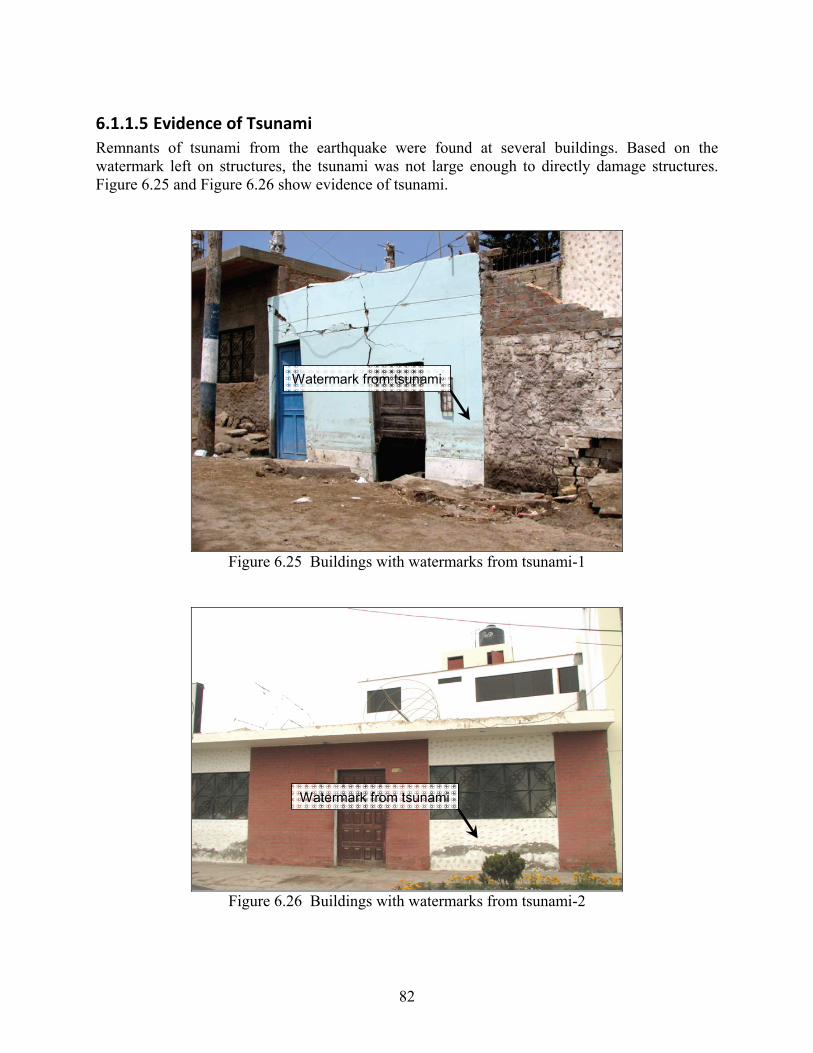
82
6.1.1.5 Evidence of Tsunami
Remnants of tsunami from the earthquake were found at several buildings. Based on the watermark left on structures, the tsunami was not large enough to directly damage structures. Figure 6.25 and Figure 6.26 show evidence of tsunami.
Watermark from tsunami
Figure 6.25 Buildings with watermarks from tsunami-1
Watermark from tsunami
Figure 6.26 Buildings with watermarks from tsunami-2

83
6.1.2 Tambo de Mora and Chincha Alta Chincha region, which includes Tambo de Mora and Chincha-Alta, is close to the epicenter. The epicentral distances of the two cities are about 37 km and 41 km, respectively (Figure 1.1). A total of 99 lives were lost from the Chincha region. The number of destroyed residential buildings was 20,653; the highest in Peru. Many educational facilities were damaged. The seashore of the Chincha region was heavily affected by liquefaction as described in some detail in Chapter 5. Many buildings sunk a few feet into liquefied soil. Electricity poles were severely tilted or completely toppled as foundations sunk into the supporting soil, which has liquefied. Many sand blow craters were observed in the field. Large lateral spreading was also observed after movements of surface soil. The ground motions in Tambo de Mora were not recorded as earthquake stations were not available in the town. From the hazard analysis in Chapter 3, it is expected that the PGA might have been 0.28g, with a very long duration. Figure 6.27 presents the location of the damaged structures in Figure 6.28 to Figure 6.31. In the following, damaged buildings of Tambo de Mora and Chincha-Alta are presented. Some of these buildings have been mentioned in Chapter 5 also, from a foundation viewpoint.
Fig 6.28
Fig 6.29
Fig 6.30
Fig 6.31
Zone with severe liquefaction damage
Figure 6.27 Locations of pictures shown in Figures 6.28 to 6.31 in Tambo de Mora

84
Figure 6.28 An area where most buildings were damaged due to liquefaction
Settlement to liquefied soil, about 3 feet
Figure 6.29 Masonry building that sunk 3 feet due to liquefaction
Heavily cracked floor slabs were observed in many buildings. Building walls sunk into liquefied soil. The slabs were not strong enough to resist the differential pressure. Liquefied soil left water marks on the wall, Figure 6.30. Even chairs sunk into the ground when the soil was liquefied, Figure 6.31.

85
Figure 6.30 Upheaval of floor slabs
` Figure 6.31 A chair partially buried in liquefied soil

86
Figure 6.32 Damaged hospital building in Chincha-Alta

87
6.1.3 Ica Ica is located 115 km from the epicenter in a southeast direction (Figure 1.1). The number of destroyed residential buildings in Ica is 13,813, which is the second largest from this earthquake after Pisco. Seventy-three people perished from the earthquake. The MAE Center field investigation team visited the National University in Ica to have a closer look at heavily damaged RC structures. The damage to the RC buildings at National University in Ica was caused by several factors such as short column effects from infill walls, inadequate column stirrup, and overloading. These damages will be covered more in detail in Chapter 7. In the following, some representative pictures of damaged structures are presented. In Figure 6.33, the masonry infill walls were heavily cracked after the earthquake. In other buildings, the infill walls were almost intact while columns were damaged or totally crushed. Figure 6.34 shows interior view of the damaged building in Figure 6.33 where a column is damaged by shear. In Figure 6.35 columns of the building completely lost their load carrying capacity. This building is analyzed in Chapter 7.
Figure 6.33 Damaged infill walls of a building at the National University of Ica
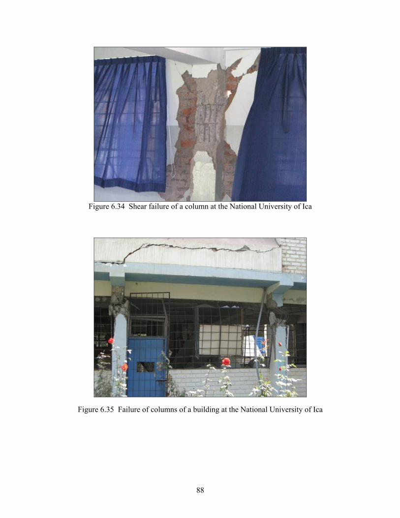
88
Figure 6.34 Shear failure of a column at the National University of Ica
Figure 6.35 Failure of columns of a building at the National University of Ica

89
Figure 6.36 Collapse of massive masonry church building
Figure 6.37 Debris from collapsed of masonry residential buildings
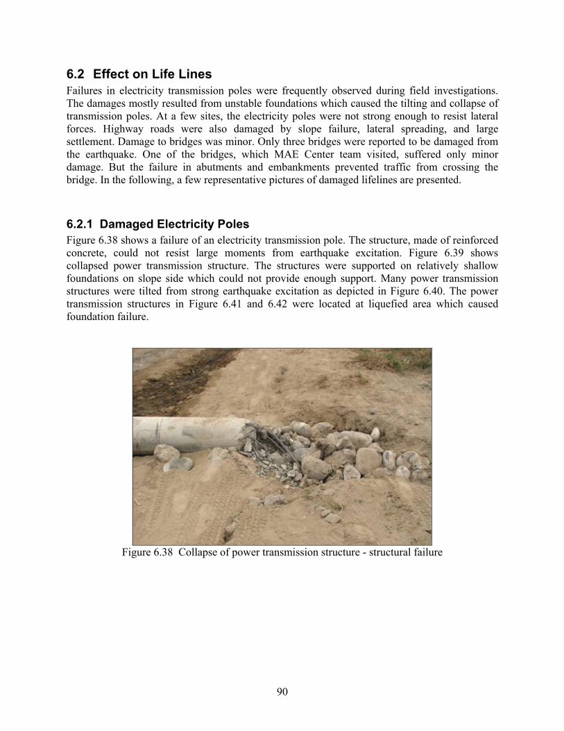
90
6.2 Effect on Life Lines Failures in electricity transmission poles were frequently observed during field investigations. The damages mostly resulted from unstable foundations which caused the tilting and collapse of transmission poles. At a few sites, the electricity poles were not strong enough to resist lateral forces. Highway roads were also damaged by slope failure, lateral spreading, and large settlement. Damage to bridges was minor. Only three bridges were reported to be damaged from the earthquake. One of the bridges, which MAE Center team visited, suffered only minor damage. But the failure in abutments and embankments prevented traffic from crossing the bridge. In the following, a few representative pictures of damaged lifelines are presented.
6.2.1 Damaged Electricity Poles Figure 6.38 shows a failure of an electricity transmission pole. The structure, made of reinforced concrete, could not resist large moments from earthquake excitation. Figure 6.39 shows collapsed power transmission structure. The structures were supported on relatively shallow foundations on slope side which could not provide enough support. Many power transmission structures were tilted from strong earthquake excitation as depicted in Figure 6.40. The power transmission structures in Figure 6.41 and 6.42 were located at liquefied area which caused foundation failure.
Figure 6.38 Collapse of power transmission structure - structural failure
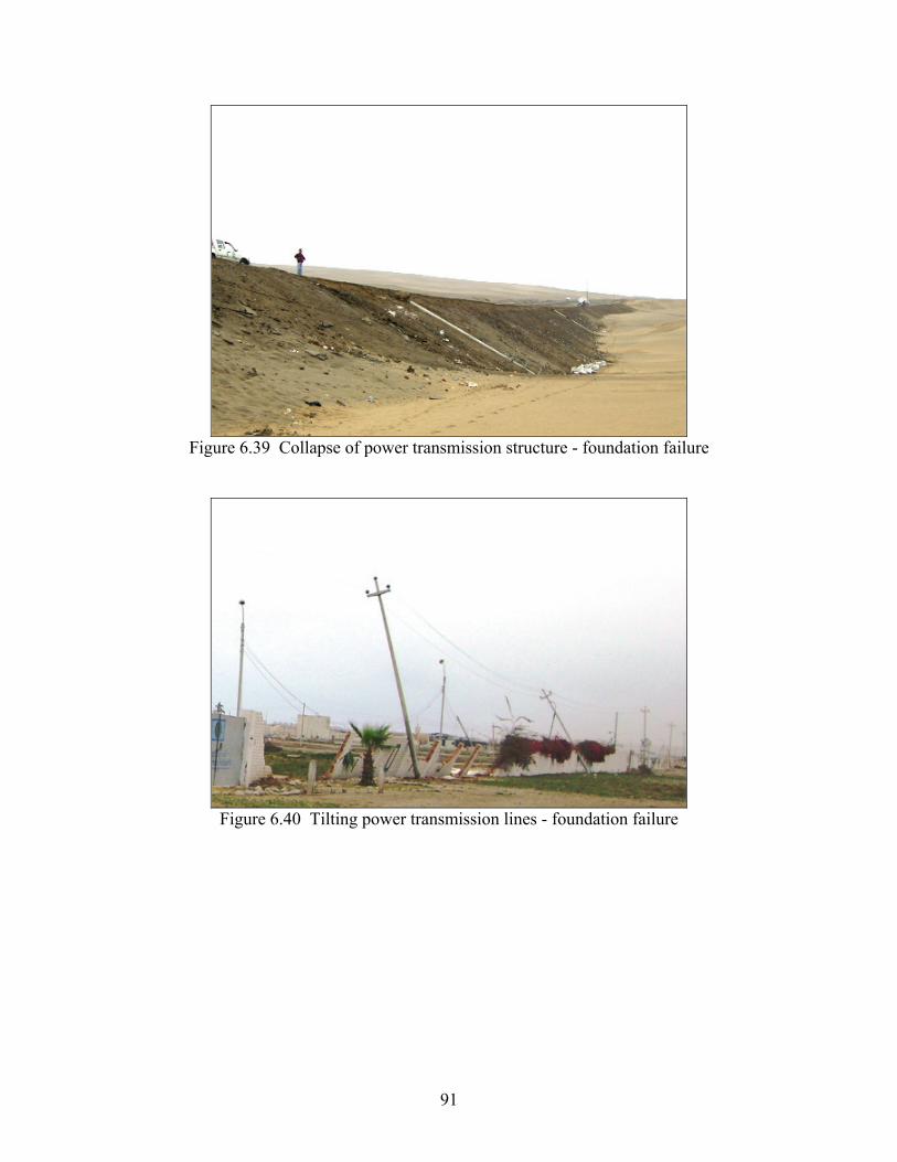
91
Figure 6.39 Collapse of power transmission structure - foundation failure
Figure 6.40 Tilting power transmission lines - foundation failure

92
Figure 6.41 Collapse of power transmission lines
Figure 6.42 Collapse of power transmission lines

93
6.2.2 Road Failure It was reported that several road segments were not functional due to slope failure, lateral spreading, and large settlement. When the field investigation team was visiting the site two weeks after the earthquake, most roads were temporarily fixed allowing traffics. Figure 6.43 to 6.46 shows typical failure mode of roads from the Pisco-Chincha Earthquake. Note that pictures in Figure 6.43 to 6.46 were taken by researchers in CISMID before the arrival of MAE Center field investigation team.
Figure 6.43 Slope failure and damage to highway
Figure 6.44 Road failure from lateral spreading perpendicular to the road

94
Figure 6.45 Road failure from lateral spreading parallel to the road
Figure 6.46 Road failure from slope failure

95
6.2.3 Bridge Failure Embankments and abutment at both ends of bridge in Figure 6.47 were damaged from the earthquake. Due to the failure of fills at approach embankments, there was large gap between bridge abutment and connecting road. Superstructure of the bridge was almost intact. The substructure of the bridge consists of large pier with shear keys which were damaged from the earthquake, Figure 6.48.
Figure 6.47 Abutment and embankment failure
Figure 6.48 Damage to shear key of a bridge
96
6.3 Reinforced Concrete Structures
6.3.1 Introduction The most severely damaged areas during the Pisco-Chincha Earthquake were the cities of Ica, Pisco and Chincha, located in the Ica Region. During the MAE Center field mission, different structural problems were observed. Many non-engineered as well as some engineered structures suffered devastating damage. The majority of the structures in these cities are one or two-story residential buildings, three to five story apartments, public and commercial buildings, schools and hospitals. The observed damages in these structures were due to several causes, which will be briefly introduced in the following.
6.3.2 Description of Materials, Construction and Systems The use of Reinforced Concrete (RC) to build small houses is not common in Peru, due to its high costs compared to other construction materials. Most residential buildings are built economically with adobe masonry or with brick masonry with small RC bracing elements for the middle and upper classes. Thus, building materials are related to economic class levels in Peru. RC structures in Peru are used for medium to high rise buildings, mainly due to its relative cost in comparison with steel structure. The low cost of RC structures in Peru can be attributed to several reasons: cheap workmanship, the use of easily acquired stones and sand as ingredients, and the use of country-wide industrial materials like cement and steel bars. Taking into account the high resistance of RC structures against earthquake, if designed and constructed properly, compared to other low cost construction materials, like masonry or wood, it is natural that RC is used for medium to high importance structures.
6.3.3 Observed Damage Patterns and Implications
6.3.3.1 Short‐Column Failure Mode
This failure mode, also called captive-column or captured-column, is very common in RC frames with infill walls. This failure happens when an infill wall is extended into a frame from the floor level up to another level to form a window, leaving a short free space in the top portion. The column in such a structure is partially restricted by the wall. This shortened column develops large shear force which may exceed the shear capacity of the column, resulting in failure. There were several buildings in the visited cities that showed this type of failure. The problem is well known but is often ignored in practice. In some cases, the infill walls are separated from the column to allow flexure of columns. But insufficient gaps produced the same consequences. An office building from a factory in Pisco showed extensive problems for this type of failure (Figure 6.49), and three buildings at the National University of Ica suffered severe damage due to different reasons, one of them being the short-column effect, Figure 6.50.

97
Figure 6.49 Short column failure at office building in Pisco
Figure 6.50 Detail of a failure in a column of a building
at the National University of Ica
6.3.3.2 Soft Story In some cases, architectural considerations lead to the discontinuity of walls in certain floors, forming the so-called “soft story”, which causes one story to be weaker than the others due to a reduction in stiffness. This normally happens at the ground floor of commercial buildings or residential buildings, where no walls are built, but only columns, in order to have openings for exhibition or parking places. Several buildings in Peru were collapsed due to soft story. Figure 6.51 is presented as an example of the consequences of the “soft story” irregularity in a family

98
house in Pisco. This house failed as consequence of inappropriate structural design, which consists of a rigid block in the second floor and a weak ground floor. In another case, observed in Chincha Alta (Figure 6.52), an intermediate level is affected by a soft story producing extensive damage in a three-story building.
Figure 6.51 Collapse of housing unit in Pisco due to soft story problems
Figure 6.52 Failure of a three-floor building in Chincha Alta
due to intermediate soft story

99
6.3.3.3 Irregularities – Eccentricities In Pisco Playa Town, a four-story building collapsed due to poor structural design. The architectural distribution in this case presented a combination of frames in the two facades and frames with infill walls in the property limits. The asymmetric distribution caused an excessive eccentricity between the center of mass and the center of stiffness, producing high shear forces at the ground floor resistant elements by torsion. The walls attached to the RC frames at the limits of the property increased the stiffness of these frames, developing large torsional moment (Figure 6.53 to Figure 6.54). Columns were failed due to large shear forces originated by the torsion of the building.
Figure 6.53 Collapse of building at Pisco Playa

100
Figure 6.54 View of inner columns of collapsed building at Pisco Playa

101
6.3.3.4 Infill Wall Failure
Infill walls, usually located between RC columns and beams, can suffer out-of-plane overturn due to inertial forces during an earthquake. Because infill walls are non-load-bearing elements, they tend to be thin and cannot rely on the additional shear strength that accompanies vertical compressive loads. If infill walls are not properly restrained in out-of-plane direction, walls can collapse during strong ground shaking, producing damages to inhabitants and properties. If walls on the façade of a structure collapse, the consequences could be deadly to pedestrians. Figure 6.55 through Figure 6.57 shows several RC buildings with infill wall failure.
Figure 6.55 Out-of-plane failure of infill walls in Ica

102
Figure 6.56 Falling of infill walls of housing unit in Pisco.
Figure 6.57 Tilted infill wall at the National University of Ica

103
6.3.3.5 Extension of Existing Buildings by Additional Floors During an earthquake, upper floors experience larger displacement and acceleration than lower floors. It is common in practice to build additional floors at a later stage on top of existing buildings. When these elements are not designed and constructed properly without strengthening their supporting components, their collapse can be devastating. Figure 6.58 shows the remains of an add-on element that fell from the top floor of the building. The extensive damage that this element inflicted on people and property outside of the building is clear. Medium-height buildings tend to have additional elements in the upper part, mainly for water tanks. Figure 6.59 shows the status of an added element near collapse, as an example of a dangerous result of poor engineering and construction detail.
Figure 6.58 Collapse of an extension from the top floor of a building in Pisco

104
Figure 6.59 Added element about to fall down from the top floor
of a building in Pisco.
6.3.3.6 Residential Buildings on Slopes On the route from Lima to Pisco on South Pan-American Highway, there is a residential complex which was developed on sand slope (Figure 6.60). These housing units, which belong to wealthy residents, are used mainly during the summer season. The soil conditions are not suitable for this type of structure because it is a steep slope of uncompacted sand, which does not offer good stability. Some of these structures collapsed during the Pisco-Chincha earthquake.

105
Figure 6.60 Collapsed buildings due to slope instability
6.3.4 Peruvian Code NTE E.030 In 1997, a new version of the Peruvian Seismic Resistant and Design Code NTE.030 was approved, which replaced the first version approved in 1977. This new version introduced a number of important changes which, according to the perception of the Specialized Technical Committee, have helped to reduce the damage to buildings—such as the damage observed in the earthquake of Atico, in June 2001. In 2003, the code was revised with minor changes. In the revised version, lateral displacement limit under earthquake load is reduced to control building damage. During the Pisco Earthquake, it was shown that the buildings designed and constructed according to the current Seismic Code behaved very well. This demonstrates that proper application of the Seismic Code and good engineering practices are required to ensure safety of structures. The Embassy Hotel in Pisco Playa was an RC building designed and built without engineering considerations. This building did not meet the code requirements, nor did it follow good constructive practices, and consequently it collapsed (Figure 6.15). On the opposite side, housing units, schools and Hospitals buildings, properly designed and constructed following the Peruvian Seismic Code, exhibited good seismic behavior during the Pisco earthquake. These cases show that the current Code can provide safety design provisions for buildings (Figure 6.21 to Figure 6.23).

106
7 Case study: Ica University Building Analysis
7.1 Location and Recorded Ground Motion The reference structure is located at Ica, Peru, 117 km from the epicenter of Pisco-Chincha Earthquake, Figure 7.1. In Ica, many residential structures constructed with adobe and masonry were heavily damaged. Most engineered structures survived the earthquake without significant damages. However some of the engineered structures, including the one investigated in this study, suffered significant damages. The building in this study was selected as it was an engineered structure and heavily damaged during the earthquake. Furthermore, recorded ground motions were available from a nearby ground motion station (ICA2) 0.5 km away from the building. Hence the observed structural damage can be understood through a nonlinear response history analysis with the actual input ground motion.
Epicenter
Ica
117 km
GM Station, ICA2
Reference Structure
0.5 km
Figure 7.1 Location of the reference structure
An analog accelerometer was used to record the motion and was on the first floor of a two story building similar to the reference structure, Figure 7.2. As the accelerometer was not installed on bedrock, it was anticipated that the recorded ground motions might include vibration components resulting from soil-structure interaction. Hence in the analysis in this study, soil structure interaction is not explicitly accounted as it is implicitly considered by applying recorded ground motion at the first floor of the similar building.

107
Figure 7.2 ICA2 station with analog accelerometer
7.2 Configuration of the Reference Building The reference building was used as a class room and a chemistry lab. The building was a two story reinforced concrete structure and consisted of 12 bays in EW direction and 3 bays in NS direction, Figure 7.3. The building was constructed as two independent modules separated at the center of EW direction. Two modules had completely independent gravity load carrying system by separation of slabs and beams at the interface of two modules. Stair wall was also an independent module. Spans of each bay were 4.2 m x 8.0 m. At the east and west face of the building, additional columns (CW21~23 and CE21~23) were constructed on the first floor to support gravity loads of full-height infill walls on the second floor, Figure 7.3(a). Figure 7.4 illustrates the west and north face elevation of the building. Exterior walls facing east and west were story-high infill walls, Figure 7.4(a). Partial height infill walls were placed between most columns in north and south face of the building, Figure 7.4(b). Most of them had openings for windows. Some of the infill walls had openings used for entrances. Infill walls were made of clay bricks with 175 mm thickness. The second floor slabs were extended as cantilevers. Cladding was constructed on top of the cantilevered slabs to expand usable floor area. Story heights for the both floors were 4.1 m. Column dimension of the building were 350 mm x 550 mm for all columns except intermediate columns in west and east face. Eight #5 (diameter = 15.8 mm) longitudinal reinforcement bars were used for exterior columns and four #5 bars were used for interior columns. Minimal amount of stirrups were used in columns; only one #3 (diameter = 9.52 mm) stirrup was used at the end of column and thin smooth wires with 5 mm diameter were used to hold longitudinal rebars in place. Beams were 350 mm x 650 mm including slab of 250 mm thickness. Rebars of beams and slabs could not be measured as those were not damaged from the earthquake.

108
Built condition
CW21, CW22, CW23, CE21, CE22, CE23: 350x480All other columns: 350x550
Ext. columns: 8 #5 longitudinal rebars (d=15.8 mm)Int. columns: 4 #5 longitudinal rebars (d=15.8mm)Stirrups: 1 #3 at the end of column
NN
Elevation 2Elevation 2
Ele
vatio
n 1
Ele
vatio
n 1
Analytical representation in Section 8.
4000
4000
3750
3750
4000
4000
4200 4200 4200 4200 4200 4200 4200 4200 4200 4200 4200 4200
CW01 CW02 CW03 CW04 CW05 CW06 CW07
CW21
CW08 CW09 CW10 CW11 CW12 CW13 CW14CE15 CE16 CE17 CE18 CE19 CE20
CW22
CW15 CW16 CW17 CW18 CW19 CW20
CW23
CE07 CE09 CE10 CE11 CE12 CE13 CE14
CE23
CE21
CE01 CE02 CE03 CE04 CE05 CE06 CE07
CE22
(a) 1st story floor plan
(b) 2nd story floor plan
Figure 7.3 Plan of the reference building
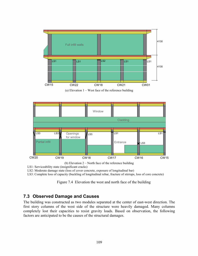
109
LS2LS1 LS1LS1 LS1
CW01CW18CW15 CW22 CW21
Full infill walls
4130
4130
(a) Elevation 1 – West face of the reference building
CW15CW16CW17CW18CW19CW20
Partial infill
Openings for window
Entrance
Cladding
Window
LS3
LS1LS3LS3LS3 LS1
(b) Elevation 2 – North face of the reference building
LS1: Serviceability state (insignificant cracks) LS2: Moderate damage state (loss of cover concrete, exposure of longitudinal bar) LS3: Complete loss of capacity (buckling of longitudinal rebar, fracture of stirrups, loss of core concrete)
Figure 7.4 Elevation the west and north face of the building
7.3 Observed Damage and Causes The building was constructed as two modules separated at the center of east-west direction. The first story columns of the west side of the structure were heavily damaged. Many columns completely lost their capacities to resist gravity loads. Based on observation, the following factors are anticipated to be the causes of the structural damages.

110
7.3.1 Short Column Effects due to Infill Walls Partial infill walls were constructed between columns in EW direction. Some of the infill walls experienced minor cracks and crushing at the corners. But most infill walls remained intact. The damage pattern of columns showed that the infill walls shortened effective length of columns. The shortened columns reduce structural periods, which in general increase seismic force demand. In addition, the shortened columns are subject to non-ductile shear failure rather than ductile flexural failure. Figure 7.5 shows examples of the column failure from the earthquake. It can be noted from Figure 7.5 (a) that the cover concrete has completely fallen off, core concrete is crushed, and longitudinal rebars are buckled. The damage pattern also shows that it failed due to flexure-axial interaction. On the other hand, Figure 7.5 (b) shows a shear failure of a column. The left side of the column is in contact with a higher infill wall than the right side of the column, significantly restricting flexural deformation toward the left. The difference in the height of infill walls forces non-symmetric deformation capacity of the column. Hence, shear cracks were developed in one direction. It can be easily noted from the marked damage patterns in Figure 7.4 that columns with less restraint from infill walls, CW15 and CW17, suffered less damage than columns with larger restraint. Additional pictures of failed columns are presented in Figure 7.5 (c)-(f).
(a) Moment-axial interaction failure, CW16 (b) Shear failure, CW18
Figure 7.5 Column damages due to infill wall restraint - contd.

111
(c) Shear failure, CW03 (d) Shear failure, CE19
(e) Shear failure, CW11 (f) Shear failure, CW06
Figure 7.6 Column damage due to infill wall restraint
7.3.2 Inappropriate Stirrups Damaged columns exposed diameters and a number of longitudinal bars as well as those of stirrups. Figure 7.7 shows a close-up view of the damaged columns, which revealed stirrups and longitudinal reinforcements. It can be clearly seen that in most columns, smooth wires with diameters of 5 mm or less were used instead of regular deformed reinforcements. The

112
longitudinal bars buckled as the weak stirrups couldn’t provide enough confinement. In addition, the number of stirrups was not large enough to provide resistance to shear force demand. The combination of increased shear force demand from column shortening with reduced shear capacity and ductility from inappropriate stirrups are the most likely cause of the column failures.
Wire ►
(a) Column, CW06 (b) Column, CW16
(c) Column, CW19 (d) Column, CW05
Figure 7.7 Stirrups of damaged columns

113
7.3.3 Overload on the Second Floor The columns in the west module were much more severely damaged than those in the right module, even though the layout of columns and beams were almost identical. Columns CW04, CW05, CW06, and CW07 in particular were severely damaged and shortened due to loss of core concrete, Figure 7.8. A closer look at the plans of the second floor and load carrying system revealed that the columns of the west module might have been overloaded in comparison with those of the right module. The west and east face of the building had intermediate columns between major columns to support the gravity load of full infill walls on the second floor, Figure 7.4 (a). Hence, it is expected that if there is significant dead load equivalent to the infill wall of full story height, the dead load should be distributed to additional columns. From observation of the building, however, it was found that the span surrounded by columns, CW06, CW07, CW14, and CW13, was heavily overloaded with partition walls as shown in Figure 7.4 (b). In addition, there was fairly high cladding on the canopy of the overloaded span, Figure 7.8. These gravity loads seem to be larger than the full-height infill walls on the east and west face. Hence the columns of this span may have carried larger gravity loads than design loads. Crushing and shortening of the columns of this span might have redistributed gravity loads over other columns resulting in subsequent failure of columns.
Figure 7.8 Overloaded span of the building

114
7.4 Back Analysis of the Reference Structure Nonlinear analyses of the damaged structure are presented in this section. The columns and beams of the structure are modeled with fiber based section elements in Zeus-NL (Elnashai et al., 2002). Infill walls are modeled as diagonal struts whose hysteretic properties are determined based on methods in literatures. The followings are assumed in the analytical model of the structure.
Infill walls do not carry vertical loads. This assumption is adopted as infill walls were constructed after frames were constructed. In addition, most of the infill walls of the building had openings for windows, which did not allow transfer of gravity loads from beams to infill walls.
Infill walls can be represented by diagonal struts with horizontal resistance. The two modules of the building vibrate independently. Hence only west part of the
building is modeled.
Nonlinear response history analyses are conducted to evaluate the shear force demand on the 1st story columns of the building. Effects of infill walls are also studied by comparison of analytical results of a frame without infill walls. The following analyses are conducted in this study.
Pushover analysis o Building with as-is condition o Building without infill walls
Nonlinear response history analysis o Building with as-is condition o Building without infill walls
In the following section, details of analytical models and results are presented.
7.4.1 Analytical Model
7.4.1.1 Reference Frame
The shaded frame on the west module of the building in Figure 7.3 (a) is modeled for numerical analyses. The analytical model has six bays and two stories, Figure 7.9. Infill walls are modeled as diagonal struts whose hysteretic properties will be introduced in the later part of this section.
CW01 CW02 CW03 CW04 CW05 CW06 CW07
Fiber section columns and beams
Rigid struts with hysteretic springs at the end
Figure 7.9 Analytical model of a reference frame

115
7.4.1.2 Material Properties
The material properties of the concrete and steel reinforcements were not able to be obtained from the field investigation. Thus the strengths of concrete and steel reinforcements are assumed based on typical material properties. Concrete ultimate strength is assumed to be 27 MPa and steel yield strength is assumed to be 410 MPa.
7.4.1.3 Beam and Column Sections
Dimensions of column and beam sections were obtained from the field investigation. The diameters and number of longitudinal and transverse reinforcements of columns were measured from field and are as shown in Figure 7.10.
All longitudinal rebars: #5 (d=15.8mm)
All stirrups: d=5 mm @350mm
Section C1 Section C2 Section C3
Section C1: CW21, CW22, CW23, CE21, CE22, CE23 Section C2: CW01~08, CW14~20, CE01~08, CE14~20 Section C3: CW09~13, CE09~13
Figure 7.10 Section dimensions of columns
Sections of beams are modeled as T-beams to account for the effect of slabs. The effective flange width is assumed to be the smallest of 1/4 of beam length (2000 mm), 16 times the slab thickness (4000 mm), and a clear distance from web to adjacent web (4200 mm) as proposed in concrete design code, ACI 2002. The reinforcements of beams were not able to be observed from field investigation as none of them were exposed after the earthquake. Thus the reinforcements are determined from design of the T-beam under gravity load. It can be easily noted that the section size of beam is substantially larger than that of columns. Figure 7.11 illustrates layout of reinforcements at the ends of beams.

116
All longitudinal rebars: 3#5 (d=15.8mm) at top2#5 at bottom
All stirrups: #3 (d=10 mm) @300mm
Figure 7.11 Section dimensions of beams
7.4.1.4 Infill Walls
Masonry walls can be modeled with two diagonal compression struts, Madan, 1997. The strengths of the struts are determined based on the possible failure modes of infill walls. There are several potential failure modes for infill masonry walls (Paulay and Pristley, 1992) including:
Sliding shear failure of masonry walls, Compression failure of diagonal strut, Diagonal tensile cracking, and Tension failure mode (flexural).
Among the above failure modes, the first and the second failure modes are most common. In this study shear strengths for the first and the second modes are evaluated for each infill wall, and the minimum of the two is considered to be the ultimate strength of infill walls. Compression strength of masonry prism is a key parameter in the estimation of the properties of the diagonal struts. Paulay and Pristley (1992) proposed an equation for the estimation of the compression strength of masonry prism.
' ' '
'
' '
cb tb j
m y
u tb cb
f f ff f
U f f
(7.1)
where = / 4.1j h h = height of the masonry unit j = thickness of mortar
uU = 1.5, stress nonuniformity coefficient '
tbf = tension strength of brick, 0.1 'cbf
'cbf = compression strength of brick,
'jf = mortar compression strength

117
The above equation needs material parameters of brick and mortar, both of which are not available for the reference building. Loaiza and Blondet (2002) report that the strength of masonry prism of typical masonry walls in Peru is 13~16 MN/m2. In this study, it is assumed that the compression strength of masonry prism is 14.5 MN/m2. Shear strength for sliding shear failure mode can be defined as below, following Mohr-Coulomb failure criteria:
f o N (7.2)
where o = cohesive capacity of the mortar beds
= sliding friction coefficient along the bed joint
N = vertical compression stress in the infill wall
In terms of force,
f o mV tl N (7.3)
where t = infill wall thickness ml = length of infill panel, Figure 7.12
N = vertical load in infill walls. As there is no external load, N can be approximated as vertical component of the diagonal compression force, sincR
cos sinc o m cR tl R (7.4)
or, 1 tan
o mf
tlV
(7.5)
Typical ranges for these parameters are 0.1 1.5o MPa and 0.3 1.2 , Mostafaei and Kabeyasawa (2004). For evaluation analysis purposes, it may be assumed that
'0.04 0.04(14.5) 0.58o mf MPa (Paulay and Pristley, 1992).
Figure 7.12 Infill masonry walls and the equivalent diagonal strut parameters Mostafaei and Kabeyasawa (2004)
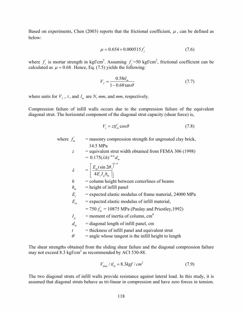
118
Based on experiments, Chen (2003) reports that the frictional coefficient, , can be defined as below:
'0.654 0.000515 jf (7.6)
where '
jf is mortar strength in kgf/cm2. Assuming 'jf =50 kgf/cm2, frictional coefficient can be
calculated as 0.68 . Hence, Eq. (7.5) yields the following:
0.58
1 0.68 tanm
f
tlV
(7.7)
where units for fV , t , and ml are N, mm, and mm, respectively.
Compression failure of infill walls occurs due to the compression failure of the equivalent diagonal strut. The horizontal component of the diagonal strut capacity (shear force) is,
' cosc mV ztf (7.8)
where '
mf = masonry compression strength for ungrouted clay brick,
14.5 MPa z = equivalent strut width obtained from FEMA 306 (1998)
= 0.40.175( ) mh d
=
1/ 4
sin 2
4m
c g m
E t
E I h
h = column height between centerlines of beams mh = height of infill panel
cE = expected elastic modulus of frame material, 24000 MPa
mE = expected elastic modulus of infill material,
= 750 'mf = 10875 MPa (Paulay and Priestley,1992)
gI = moment of inertia of column, cm4
md = diagonal length of infill panel, cm
t = thickness of infill panel and equivalent strut = angle whose tangent is the infill height to length The shear strengths obtained from the sliding shear failure and the diagonal compression failure may not exceed 8.3 kgf/cm2 as recommended by ACI 530-88.
2
max / 8.3 /mV tl kgf cm (7.9)
The two diagonal struts of infill walls provide resistance against lateral load. In this study, it is assumed that diagonal struts behave as tri-linear in compression and have zero forces in tension.

119
Ideally, the resistance of the infill walls after failure should be smaller than maximum resistance, strength and stiffness degradation may occur for repeated cycles, and sliding may happen. As the field observation showed that infill walls rarely damaged, tri-linear hysteretic curves are adopted for infill walls’ hysteretic model.
U
V
Uy Um
Vy
Vm
Compression
Tension
K0
αK0
Figure 7.13 Diagonal masonry walls and the equivalent diagonal strut parameters
The tri-linear displacement-force envelope consists of parameters such as Vy, Vm, Uy, and Um. The maximum displacement at the maximum lateral force is estimated by Eq. (7.10), Madan (1997).
'
cosm m
m
dU
(7.10)
where '
m is the masonry compression strain at the maximum compression stress, here ' 0.0018m and md is the diagonal strut length. The maximum drift limitation of 0.8% is
applied for the /m mU h ratio, which is implied from the experimental results, Mehrabi et al. (1996) and Chen (2003).The initial stiffness oK is estimated as following, Mandal et al. (1997):
0 2( / )m mK V U (7.11)
where mV is the maximum strength determined from Eq. (7.7), (7.8), and (7.9). The post yield stiffness ratio, , is assumed as 0.2. The parameters, yU and yV , can be estimated from geometry.
7.4.1.5 Gravity Loads and Mass
The gravity load is estimated from the dimension of slabs, beams, and infill walls as below.
Density of concrete 2400 kg/m3 Element Mass per unit length or area Slab Thickness: 0.25m 600 kg/m2 Beam (without slab) area: 0.14 m2 336 kg/m Infill wall Thickness: 0.175 m Height (partial): 1.32 m 554.4 kg/m Height (partial): 2.28 m 958 kg/m

120
Height (full): 3.48 m 1462 kg/m Cladding Section area: 0.3 m2 720 kg/m Column Area (350x480) 0.168 m2 403 kg/m Area (350x550) 0.193 m2 463 kg/m
Total mass of the structure is 212 tons. The mass is lumped at beam and column joints on the first and second floor.
7.4.1.6 Damping
Damping ratio for reinforced concrete structures is commonly taken as 5% of critical damping for elastic analysis. When a structure behaves in a nonlinear range, the hysteretic behavior of materials dissipates energy. Thus, assuming the same amount of damping for elastic and inelastic systems is not reasonable (Kwon and Elnashai, 2006). In the response history analysis of the reference building, 2% of damping at the fundamental period of the structure is assumed.
7.4.2 Pushover Analysis Pushover analyses of two frames, with infill wall and without infill wall, are conducted. Figure 7.14 shows the pushover curves of the two frames. The frame with infill wall has larger stiffness and strength. A peak base shear coefficient of 0.38 is obtained at the roof displacement of 171 mm. Most of the roof drift is developed from deformation of the second floor, Figure 7.15. The base shear coefficient of the frame without infill wall is 0.27 at roof displacement of 97 mm where large deformation occurs at the first floor. Deformed shapes and pushover curves show that the frame with infill wall is stronger and that damage is concentrated on the second floor. This analytical result from pushover analysis does not coincide with the observed failure modes from the field investigation. The main source of discrepancy is that shear deformation and shear failure of frame members are not accounted for in the analytical model. To overcome the limitation, shear capacity of columns are compared with the shear demand on the columns in the response history analysis. This approach is approximate in a sense that the shear deformation and failure are not incorporated into analysis procedure. But this approximation at least can indicate relative values of seismic demand and capacity between frame with infill walls and without infill walls.

121
0
100
200
300
400
500
600
700
800
900
0 20 40 60 80 100
Roof drift, mm
Bas
e sh
ear,
kN
w/ infill wall
w/o infill wall
0.10
0.20
0.30
0.40
0.35
0.25
0.15
0.05
Base sh
ear coefficien
t
Figure 7.14 Base shear - roof displacement from pushover analysis
(a) Frame with infill wall
(b) Frame without infill wall
Figure 7.15 Failure mode of frames from pushover analysis
7.4.3 Inelastic Response History Analyses The fundamental periods of the two frames are 0.26 sec and 0.37 sec from eigen value analysis. Nonlinear response history analyses are conducted with infill walls and without infill walls. The E-W component of the recorded ground motion at ICA2 station (Figure 4.1 (a)), is applied to the frame. The ground motion is not scaled. The frame without infill wall experiences much larger interstory drift at the first floor than the

122
interstory drift of frame with infill wall, Figure 7.16. On the second floor, the interstory drift of frame with infill wall is larger than that of frame without infill wall. This observation is close to the failure modes from pushover analysis in Figure 7.15. Shear force demands on the first story columns are compared in Table 7.1. Note that shear force demands on the frame with infill wall is up to 50% higher than the demands on the frame without infill wall. The shear capacity of the column can be calculated as below, following ACI design guidelines. In the shear capacity calculation, the contribution of stirrups is ignored as the stirrups are very widely spaced and smooth wires with diameters of 5 mm or less are used in the construction. Shear capacity provided by concrete for the Column CW06 is
'2 12000
uc c w
g
NV f b d
A
(7.12)
Where, 404uN kN , axial load on the column
20.193gA m , gross section of column
2/ 634.9 / 92.08u gN A kN m psi .
2 1 92.08 / 2000 3916 (21.65)(11.8) 33446 149cV lb kN
The shear force demand of frame with infill wall in Table 7.1 is very close to or larger than shear capacity of the column. On the contrary, the shear force demand of frame without infill wall is much smaller than the shear force capacity.
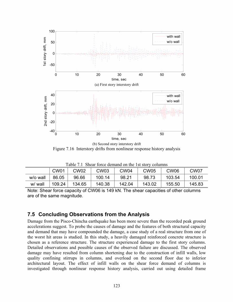
123
0 10 20 30 40 50 60
-50
0
50
100
time, sec
1st
stor
y dr
ift,
mm
with wall
w/o wall
(a) First story interstory drift
0 10 20 30 40 50 60-40
-20
0
20
40
time, sec
2nd
stor
y dr
ift,
mm
with wall
w/o wall
(b) Second story interstory drift
Figure 7.16 Interstory drifts from nonlinear response history analysis
Table 7.1 Shear force demand on the 1st story columns
CW01 CW02 CW03 CW04 CW05 CW06 CW07
w/o wall 86.05 96.66 100.14 98.21 98.73 103.54 100.01
w/ wall 109.24 134.65 140.38 142.04 143.02 155.50 145.83
Note: Shear force capacity of CW06 is 149 kN. The shear capacities of other columns are of the same magnitude.
7.5 Concluding Observations from the Analysis Damage from the Pisco-Chincha earthquake has been more severe than the recorded peak ground accelerations suggest. To probe the causes of damage and the features of both structural capacity and demand that may have compounded the damage, a case study of a real structure from one of the worst hit areas is studied. In this study, a heavily damaged reinforced concrete structure is chosen as a reference structure. The structure experienced damage to the first story columns. Detailed observations and possible causes of the observed failure are discussed. The observed damage may have resulted from column shortening due to the construction of infill walls, low quality confining stirrups in columns, and overload on the second floor due to inferior architectural layout. The effect of infill walls on the shear force demand of columns is investigated through nonlinear response history analysis, carried out using detailed frame
124
analysis procedure using recorded ground motion at a nearby station. The results clearly show that the shear force demand on a frame with an infill wall is much higher than the demand on a frame without infill walls. In addition, the shear force demand on a frame with an infill wall is close to or larger than the shear force capacity approximately calculated with ACI design guideline. The study employs investigation tools, from modeling assumptions to strong-motion selection, that are of general applicability to the forensic study of damaged structures in earthquake regions.

125
8 Summary and Recommendations
8.1 Summary of observations and lessons learned Conclusions have been drawn in the various chapters above on engineering seismology, geotechnical and structural earthquake engineering. Here, a summary of the main conclusions is reiterated in order that important lessons from this earthquake are learned, towards the objective of reducing the impact of future earthquakes in Peru and elsewhere. The earthquake occurred in an area that is very well studied and largely understood, along an
identified seismic gap of about 150 km parallel to the coast of central Peru. The magnitude of the earthquake is similar to previous confirmed earthquakes in the subduction region defined by the under-thrusting oceanic Nazca plate and the overriding South American continental plate.
There were two main events with origin time about 60 seconds apart; the second event seems to be somewhat stronger than the first rupture.
Aftershock activities are clustered in three regions indicating that this earthquake resulted from a multiple and complex rupture process.
The strong-motion available to the reconnaissance team, largely peak ground parameters from 16 stations and one high quality record from the ICA2 station in the City of Ica, indicate exceptionally high energy release.
The one strong-motion record analyzed has some interesting features in terms of duration, energy flux and RMS of acceleration, velocity and displacement.
The record was compared with records from Loma Prieta (USA, 1989), Northridge (USA, 1994), Hyogo-ken Nanbu (Japan, 1995) and Kocaeli (Turkey, 1999) with the same pga. The Pisco-Chincha earthquake record from ICA2 station has over twice the Arias Intensity, 8 to 30 times the energy flux, 2-4 times the duration and more than double the RMS of ground motion parameters. The only exception is the Kocaeli (Duzce) record which exhibits similar trends but still falls short on all comparison parameters.
The above comparison indicates that the shaking imposed on structures in the coastal region of central Peru was significantly more intense than that of many or most of the recent earthquakes.
The elastic and inelastic spectra of the record indicate that the E-W component had a much wider frequency content corresponding to high amplifications, whilst the N-S component had higher amplification, but in a relatively narrower frequency range. The average amplification for both is about 2.5-2.7 in the E-W direction (almost normal to the fault), and up to 4.0-4.2 in the N-S direction (parallel to the fault). The E-W amplification is normal, while the N-S amplification is more about 80% higher than the average amplification observed in many earthquake records.
Out of the 16 sets of peak ground parameters, 10 gave an E-W component higher than the N-S, 2 gave equal values and 4 gave lower values. It may be concluded that the E-W component has probably inflicted more damage than the N-S component, due to its higher values and wider frequency content.
Detailed comparison between the available values of peak ground parameters and calculations from the most recent and widely accepted attenuation relationships yielded a mixture of results. In some cases, very good correlation was observed. In others, the attenuation relationship over-estimated the observed ground acceleration by large margins.

126
On the whole, the attenuation relationship gave reasonable results, even though the model was derived without consideration of subduction regimes.
Geotechnical effects were overwhelming in this earthquake. A very substantial percentage of structurally damaged and collapsed buildings are a direct consequence of geotechnical, not structural, effects.
Liquefaction, both under structures and free-field, has occurred en masse. Several sand boils were observed by the reconnaissance team, some of several meters diameters.
Extensive liquefaction in Tambo de Mora caused heavy damage and collapse of almost every building in two streets, both parallel to the sea shore.
The resort of Las Lagunas near Lima has been hit hard with tens of luxurious villas sinking into the ground. This observation serves as a reminder of the perils of building on soft ground close to natural or artificial lakes that reduce the lateral ground pressure that would have otherwise reduced lateral spreading.
Few transportation structures and facilities have suffered damage. However, those hardest hit, albeit few, are critical components of the transportation system. The damage to the Huamani Bridge and several sectors of the Pan-American Highway crippled the road communication between Lima and the hardest hit areas for some days.
Extensive damage was inflicted on a small number of road segments of the Pan-American Highway, mainly due to lateral spreading and other forms of permanent ground displacement.
The Port at San Martin was damaged extensively due to settlement and large permanent ground deformation.
The electricity transmission network was one of the hardest, if not the hardest, hit utility. Many tens of electricity transmission poles failed, almost exclusively due to soil and foundation failure, not due to structural vibrations.
Masonry structures behaved on the whole very poorly. Hundreds of cases of corner collapse, diagonal cracking and shear failure at doors and openings were observed.
Use of confined masonry was scarce. Where used, confined masonry behaved well. Well designed reinforced concrete structures, the dominant construction type in recent years
in Peru, behaved very well. Countless cases were noted of severe damage and collapse of RC structures due to the often-
observed features of soft storey, unconfined columns, weak beam-column connections, short column, discontinuous load path and inferior architectural design that imposes severely varying demands on adjacent structural members.
Most of the lessons learned from this earthquake are a repeat of lessons that should have been learned from previous earthquakes, both in Peru and worldwide. It is emphasized herein that structures, their foundations and the soil surrounding these foundations are a single interacting system and should be designed and constructed as such. Perfectly adequate structures were severely damaged or collapsed because of soil and/or foundation failure in this earthquake. The challenge that leads to such failures is the inter-disciplinary dialogue that is required across groups who are yet to establish a common vocabulary. Perhaps this is the most significant, albeit repeated, lesson from the Pisco-Chincha earthquake.

127
8.2 Recommendations The Pisco-Chincha earthquake hit an area that has exhibited one of the highest seismic activities worldwide. It would have been expected that the region is significantly more prepared than has been observed by the MAE Center reconnaissance team. Economic constraints and other social and political considerations remain somewhat of an obstacle in the way of preparing for the next earthquake, which is an inevitable occurrence. Below are some general and specific recommendations that the MAE Center and its partners puts forward for consideration by the relevant authorities in Peru.
8.2.1 Hazard It is of utmost importance for Peru and the earthquake engineering community worldwide
that the instrumentation program is expanded and accelerated. It is a historically lost opportunity to gather records from the hardest hit locations, where no recording stations existed, for scientific investigation and better understanding of one of the most seismically active regions in the world.
It should be mandatory that agencies operating strong-motion networks release without restriction all recorded ground motion, otherwise international interest drops, and the rare opportunity to pool expertise to understand the earthquake and its effects is lost.
Immediate launch of extensive efforts to increase substantially the bore hole investigation activities at important sites, such as strong-motion stations, critical facilities, important arterial structures and power plants, in order to aid in developing ground motion models as mentioned below.
Mandatory requirement for instrumenting all new projects with a minimum of sensing stations for the collection of vital response data.
Development of a micro-zonation program for areas of special soil conditions such as the entire sea shore region, the terraced planes to its east and areas surrounding rivers and lakes further inland.
Extensive work on developing ground motion models that are particular to Peru with an emphasis on site response and soil effects.
8.2.2 Planning for Risk Management Launching of data collection effort for all assets exposed to earthquakes and development of
an extensive program for GIS inventory collection and archival. Drawing a regional assessment, mitigation, response and recovery needs. Development or adoption of a loss assessment software tool that is used in regional and
national scenario loss assessments for the purposes of planning of response, determination of required mitigation measures, stockpiling of required equipment and recruitment of necessary personnel, and articulating a detailed response and recovery plan of action.
8.2.3 Design and Construction Development of simple deemed-to-satisfy rules that are pictorially-based, without equations,
for simple structures in rural regions, including provisions for foundation reinforcement and tying.

128
Implementation of hierarchical, self-monitored, strict construction authorization procedures. This should include continuous control of all construction and concurrent penalties on defaulting, non-conforming and random housing.
Development of codes for seismic resistance of infrastructure and lifeline systems.
8.2.4 Legislation Backing up all the above by rigorous legislative structures and clear frameworks for
adherence and continuous monitoring. Legislating for a complete and comprehensive framework of emergency management
professionals at the local, regional and national levels, and a clear reporting mechanism, alongside a tiered emergency preparedness plan.
Establishing a ‘Disaster Fund’ that is used to provide regional emergency relief, and funded by a modest tax on new projects. Such funds have precedence and experience should be gained from other countries on this issue.
The above list is not comprehensive and is subject to further refinement and articulation as more information becomes available and the needs are better defined.

129
9 Acknowledgements The field mission was sponsored by the Mid-America Earthquake Center. The MAE Center is an Engineering Research Center funded by the National Science Foundation under cooperative agreement reference EEC 97-01785. CISMID (Center for Peruvian-Japanese Seismic Research and Disaster Mitigation), represented by Professor Carlos Zavala, and the Faculty of Civil Engineering at the National University of Engineering of Peru, represented by Professor Jorge Alva-Hurtado, provided logistical support and valuable information throughout the mission.

130
10 References ACI (2002). Building code requirements for structural concrete and commentary (318-02).
American Concrete Institute, Detroit, Michigan.
ACI/ASCE (1988). Building Code Requirements for Masonry Structures (ACI-530-88/ASCE 5-88) and Specifications for Concrete Institute and American Society of Civil Engineers, Detroit.
Ambraseys, N. N., Douglas, J., Sarma, S.K., and Smit, P. M., (2005a). “Equation for the Estimation of strong Ground Motions from Shallow Crustal Earthquakes Using Data from Europe and the Middle East: Horizontal Peak Ground Acceleration and Spectral Acceleration”, Bulletin of Earthquake Engineering, 3:1-53.
Ambraseys, N. N., Douglas, J., Sarma, S.K., and Smit, P. M., (2005b). “Equations for the Estimation of Strong Ground Motions from Shallow Crustal Earthquakes Using Data from Europe and the Middle East: Vertical Peak Ground Acceleration and Spectral Acceleration”, Bulletin of Earthquake Engineering, 3:55-73.
Barazangi, M. and Isacks, B.L., (1976). “Spatial distribution of earthquakes and subduction of the Nazca plate beneath South America”, Geology, 4:686-692.
Bernal, I, and Tavera, H. (2007a) Peak ground accelerations recorded at Ica District: The 2007 Pisco Earthquake, Geophysical Institute of Peru, Special Volume: The Pisco Earthquake of August 15, 2007. In Spanish.
Bernal, I., and Tavera, H. (2007b) Peak ground accelerations recorded at Lima City: The 2007 Pisco Earthquake, Geophysical Institute of Peru, Special Volume: The Pisco Earthquake of August 15, 2007. In Spanish.
BSSC (2004) NEHRP recommended provisions for new buildings and other structures (FEMA 450), 2003 Edition, Report prepared for the Federal Emergency Management Agency (FEMA). Washington, D.C.
Campbell, K. and Bozorgnia, Y. (2006) “Next Generation Attenuation (NGA-CB) Empirical Ground Motion Models: Can They be Used in Europe?, First European Conference on Earthquake Engineering and Seismology, Geneva, Switzerland, 3-8 September 2006. Paper Number: 458.
Campbell, K. and Bozorgnia, Y. (2007) Campbell-Bozorgnia NGA-CB Empirical Ground Motion Model for the Average Horizontal Component of PGA, PGV, PGD and SA at Selected Spectral Periods Ranging from 0.01–10.0 Seconds, PEER-Lifelines Next Generation Attenuation of Ground Motion (NGA-CB) Project.
Chen, Y. (2003). Seismic Evaluation of RC Buildings Infilled with Brick Walls. PhD thesis, National Cheng-Kung Univ., Tainan, Taiwan, in Chinese.
Dorbath, (1996). “Velocity structure of the Andes of Central Peru from locally recorded earthquakes,” Geophysical Research Letters, 23(2):205-208.
The Dynamic Earth. (2007, May 5). In United States Geological Survey, from http://pubs.usgs.gov/publications/text/Vigil.html.
Elnashai, A.S., Papanikolaou, V. and Lee, D. H. (2002). Zeus-NL - A System for Inelastic Analysis of Structures.

131
IGP (2001), Seismic Map of Peruvian Seismicity, Atlas of Peruvian Natural Hazards, Geophysical Institute of Peru. In Spanish.
IGP (2007). Registros De Aceleración Para Sismos Sensibles En Lima 2007. (2007, Nov 2). In Instituto Geofísico del Perú, from http://khatati.igp.gob.pe/Webs/cns06/reg_acelerac/ reg_acel_lima2007.htm.
INDECI, National Institute for Civil Defense (2007). Current Situation – Ica and South of Lima, released on 03/09/2007.
Ingemmet (1994). Estudio Geovolcánico e Inventario Sistemático de Manifestaciones Geotermales del Lote Tutupaca, Instituto Geológico Minero y Metalúrgico y ELECTROPERU, Lima, Peru.
Isaaks, E. H., and R. M. Srivastava. 1989. An introduction to applied geostatistics. Oxford University Press, New York. 561pp.
Konca, O. (2007) Slip History Database of Global Large Earthquakes, California Institute of Technology. http://www.tectonics.caltech.edu/slip_history/index.html.
Kwon, O. and Elnashai, A. S. (2006). “The effect of material and ground motion uncertainty on the seismic vulnerability curves of a RC structure,” Engineering Structures, 28(2):289-303.
Loaiza, C. and Blondet, M. (2002). World Housing Encyclopedia Report, Country: Peru, Earthquake Engineering Research Institute.
Leffler, L., Stein, S., Mao, A., Dixon, T., Ellis, M. A., Ocola, L., and Selwyn Sacks, I., (1997). ”Constraints on present-day shortening rate across eastern Andes from GPS data”, Geophysical Research letters, 24:1031-1034.
Loaiza, C. and Blondet, M. (2002). World Housing Encyclopedia Report. Country: Peru. Earthquake Engineering Research Institute.
Madan A, Reinhorn A.M., Mandar J.B., and Valles R.E. (1997). Modeling of masonry infill panels for structural analysis, Journal of Structural Engineering ASCE 123(10): 1295-1302.
Mehrabi, A. B., Shing, P. B., Schuller, M. P., and Noland, J. L. (1996). "Performance of masonry-infilled reinforced concrete frames under in-plane lateral load." Journal of Structural Engineering, 122(3):228-237.
Mostafaei, H., and Kabeyasawa, T. (2004). "Effect of Infill Masonry Walls on the Seismic Response of Reinforced Concrete Buildings Subjected to the 2003 Bam Earthquake Strong Motion: A Case Study of Bam Telephone Center." Bulletin of Earthquake Research Institue, University of Tokyo, 79:133-156.
Murrugarra , D. P., López, D. V., and Alva-Hurtado, J. E. (1999). “Microzonificación Geotécnica De Pisco,” 12th National Congress of Civil Engineering, Huanuco, Peru.
Nazca Plate. (2007, December 6). In Wikipedia, the Free Encyclopedia. Retrieved 22:47, December 11, 2007, from http://en.wikipedia.org/w/index.php?title=Nazca_Plate&oldid =176230785.
NSHMP (2007) Preliminary documentation for the 2007 update of the United States national seismic hazard maps, Draft open-file report prepared by the national seismic hazard mapping project.

132
Paulay, T., and Priestley, M.J.N. (1992). Seismic Design of Reinforced Concrete and Masonry Buildings, John Wiley & Sons, Inc.
United States Geological Survey (2008). Peru Earthquake Information. http://earthquake.usgs.gov/eqcenter/eqinthenews/2007/us2007gbcv/. Page accessed on March 1, 2008.
United States Geological Survey (2007). Peru Earthquake Information. http://earthquake.usgs.gov/regional/world/?region=Peru. Page accessed on October 1, 2007.
SeismoSignal Ver 3.2.0
http://www.seismosoft.com
Stafford, P., Strasser, F., and Bommer, J. (2008). “An evaluation of the applicability of the NGA models to ground-motion prediction in the Euro-Mediterranean region,” Bulletin of Earthquake Engineering, 6(2):149-177.
Tavera, H. (2007) Chronicle of an Announced Earthquake for the Southern Region of Central Peru, Geophysical Institute of Peru, Special Volume: The Pisco Earthquake of August 15, 2007. In Spanish.
Tavera, H., Buforn, E., (2001). “Source Mechanism of Earthquake in Peru” Journal of Seismology, 5(4):519-540.
Tavera, H., Fernandez, E., Bernal, I., Antayhua, Y., Agilero, C., Rodriguez, H., Vilcapoma, L., Zamudico, Y., Portugal, D., Inza, A., Carpio, J., Ccallo, F. and Valdivia, I., (2006). “The Southern Region of the Peru Earthquake of June 23rd, 2001,” Journal of Seismology, 10(2):171-195.
Tavera, H., Salas, H., Rodríguez, S., Perez-Pacheco, I., Parillo, R., Millones, J., Jiménez, C., and Arredondo, L. (2007) “Space distribution of the Pisco Earthquake aftershocks: Preliminary results,” Special Volume: The Pisco Earthquake of August 15, 2007, Geophysical Institute of Peru, In Spanish.
Vallée, M. (Géosciences Azur, IRD, Nice, France, [email protected]), Julien Vergoz and Jocelyn Guilbert (LDG, DASE/CEA, Paris, France) http://www-geoazur.unice.fr/ SEISME/PERU150807/note1.html. In Spanish.
Yagi (2007) August 16 Off Peru Giant Earthquake, Tsukuba University, http://www.geo.tsukuba.ac.jp/press_HP/yagi/EQ/20070816/. In Japanese.

133
Appendix A
A.1 Field Mission Members and Specialization MAE Center Team Name Affiliation Technical Role Prof. Amr S. Elnashai
Director, Mid-America Earthquake Center, University of Illinois at Urbana-Champaign
Team Leader Structural engineering and strong-motion
Dr. Oh-Sung Kwon Post-doctoral researcher, Mid-America Earthquake Center
Structural earthquake engineering Ground motion processing Detailed back-analysis
Dr. Omar Pineda Post-doctoral researcher, Mid-America Earthquake Center
Earthquake hazard analysis Documentation and reporting coordinator
Mr. Gregory Pluta NEES Facility Manager, University of Illinois
Base station support and technical report editor
Peruvian Team Name Affiliation Technical Role Prof. Jorge Alva-Hurtado
Dean of the Faculty of Civil Engineering, National University of Engineering of Peru, Lima
Team Leader Geotechnical engineering and geology
Dr. Luis Moran Yañez
Faculty of Civil Engineering, National University of Piura
Structural engineering Communications coordinator in
Guillermo Huaco Research Assistant CISMID Structural engineering Communications coordinator in
A.2 Peruvian Host Organizations CISMID, Center Peruvian-Japanese of Seismic Research and Disaster Mitigation (Centro Peruano-Japonés de Investigaciones Sísmicas y Mitigación de Desastres) Av. Tupac Amaru Nº 1150, Sector T, Puerta 7 Lima 25 - PERÚ Apartado Postal 31-250, Lima 31 Telefax (51-1)482-0777 481-0170 Universidad Nacional de Ingeniería College of Civil Engineering, Avenida Tupac Amaru Nro 210 El Rimac, Lima PE-LIMA025 Central Telefonica: (51-1)481-1070
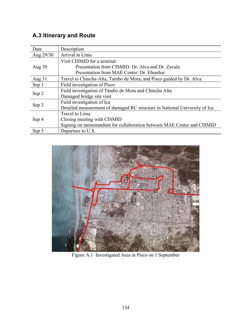
134
A.3 Itinerary and Route Date Description Aug 29/30 Arrival in Lima
Aug 30 Visit CISMID for a seminar Presentation from CISMID: Dr. Alva and Dr. Zavala Presentation from MAE Center: Dr. Elnashai
Aug 31 Travel to Chincha-Alta, Tambo de Mora, and Pisco guided by Dr. Alva Sep 1 Field investigation of Pisco
Sep 2 Field investigation of Tambo de Mora and Chincha Alta Damaged bridge site visit
Sep 3 Field investigation of Ica Detailed measurement of damaged RC structure in National University of Ica
Sep 4 Travel to Lima Closing meeting with CISMID Signing on memorandum for collaboration between MAE Center and CISMID
Sep 5 Departure to U.S.
Figure A.1 Investigated Area in Pisco on 1 September

135
Tampo de Mora
Chincha Alta
Figure A.2 Investigated Area in Tambo de Mora and Chincha Alta on 2 September
Figure A.3 Investigated Area in Ica on 3 September

136
Appendix B
B.1 Recorded ground motions and response spectra Station code : ICA2 Station name : Laboratorio de Mecánica de Suelos de la Universidad Nacional San Luis Gonzaga de Ica Latitude : -14.0887 Longitude : -75.7321 Organization : Ceresis, IGP Epicentral distance : 117 km
0 20 40 60 80 100 120 140 160 180 200
-0.2
0
0.2
time, sec
acce
lera
tion,
g
ICA2E.dat
0 20 40 60 80 100 120 140 160 180 200
-0.2
0
0.2
time, sec
acce
lera
tion,
g
ICA2N.dat
0 20 40 60 80 100 120 140 160 180 200-0.2
-0.1
0
0.1
0.2
time, sec
acce
lera
tion,
g
ICA2V
.dat

137
0 0.5 1 1.5 2 2.5 30
0.5
1
1.5
Period, sec
Spe
ctra
l acc
eler
atio
n, g
ICA2E.dat
Elastic, =5%
Ductility=2, =2%
Ductility=4, =2%
0 0.5 1 1.5 2 2.5 30
0.5
1
1.5
Period, sec
Spe
ctra
l acc
eler
atio
n, g
ICA2N.dat
Elastic, =5%
Ductility=2, =2%
Ductility=4, =2%
0 0.5 1 1.5 2 2.5 30
0.5
1
1.5
Period, sec
Spe
ctra
l acc
eler
atio
n, g
ICA2V
.dat
Elastic, =5%
Ductility=2, =2%
Ductility=4, =2%

138
Station code : ANR Station name : Asamblea Nac. De Rectores Latitude : N/A Longitude : N/A Organization : Ceresis, IGP Epicentral distance : Approximately 150 km
0 20 40 60 80 100 120 140 160 180 200
-0.05
0
0.05
time, sec
acce
lera
tion,
g
ANRL.dat
0 20 40 60 80 100 120 140 160 180 200
-0.05
0
0.05
time, sec
acce
lera
tion,
g
ANRT.dat
0 20 40 60 80 100 120 140 160 180 200
-0.05
0
0.05
time, sec
acce
lera
tion,
g
ANRV
.dat

139
0 0.5 1 1.5 2 2.5 30
0.05
0.1
0.15
0.2
0.25
0.3
0.35
0.4
Period, sec
Spe
ctra
l acc
eler
atio
n, g
ANRL.dat
Elastic, =5%
Ductility=2, =2%
Ductility=4, =2%
0 0.5 1 1.5 2 2.5 30
0.05
0.1
0.15
0.2
0.25
0.3
0.35
0.4
Period, sec
Spe
ctra
l acc
eler
atio
n, g
ANRT.dat
Elastic, =5%
Ductility=2, =2%
Ductility=4, =2%
0 0.5 1 1.5 2 2.5 30
0.05
0.1
0.15
0.2
0.25
0.3
0.35
0.4
Period, sec
Spe
ctra
l acc
eler
atio
n, g
ANRV
.dat
Elastic, =5%
Ductility=2, =2%
Ductility=4, =2%

140
Station code : CAL Station name : Dirección de Hidrografía y Navegación-Marina de Guerra del Perú Latitude (°) : -12.06 Longitude (°) : -77.15 Organization : CISMID Epicentral distance : 160 km
0 20 40 60 80 100 120 140 160 180 200
-0.1
-0.05
0
0.05
0.1
time, sec
acce
lera
tion,
g
CALE.dat
0 20 40 60 80 100 120 140 160 180 200-0.1
-0.05
0
0.05
0.1
time, sec
acce
lera
tion,
g
CALN.dat
0 20 40 60 80 100 120 140 160 180 200
-0.02
0
0.02
time, sec
acce
lera
tion,
g
CALV
.dat

141
0 0.5 1 1.5 2 2.5 30
0.05
0.1
0.15
0.2
0.25
0.3
0.35
0.4
Period, sec
Spe
ctra
l acc
eler
atio
n, g
CALE.dat
Elastic, =5%
Ductility=2, =2%
Ductility=4, =2%
0 0.5 1 1.5 2 2.5 30
0.05
0.1
0.15
0.2
0.25
0.3
0.35
0.4
Period, sec
Spe
ctra
l acc
eler
atio
n, g
CALN.dat
Elastic, =5%
Ductility=2, =2%
Ductility=4, =2%
0 0.5 1 1.5 2 2.5 30
0.05
0.1
0.15
0.2
0.25
0.3
0.35
0.4
Period, sec
Spe
ctra
l acc
eler
atio
n, g
CALV
.dat
Elastic, =5%
Ductility=2, =2%
Ductility=4, =2%

142
Station code : CER Station name : Ceresis Latitude (°) : N/A Longitude (°) : N/A Organization : Ceresis, IGP Epicentral distance : N/A
0 20 40 60 80 100 120 140 160 180 200
-0.05
0
0.05
time, sec
acce
lera
tion,
g
CERL.dat
0 20 40 60 80 100 120 140 160 180 200
-0.05
0
0.05
time, sec
acce
lera
tion,
g
CERT.dat
0 20 40 60 80 100 120 140 160 180 200-0.04
-0.02
0
0.02
0.04
time, sec
acce
lera
tion,
g
CERV
.dat
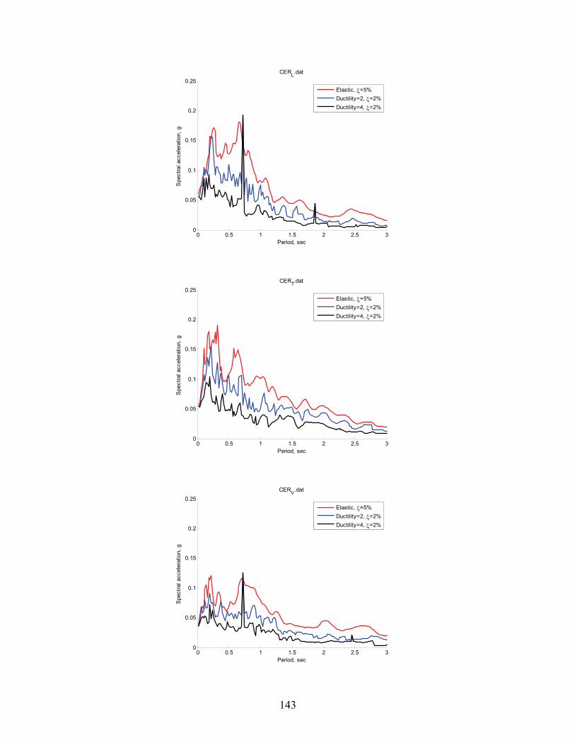
143
0 0.5 1 1.5 2 2.5 30
0.05
0.1
0.15
0.2
0.25
Period, sec
Spe
ctra
l acc
eler
atio
n, g
CERL.dat
Elastic, =5%
Ductility=2, =2%
Ductility=4, =2%
0 0.5 1 1.5 2 2.5 30
0.05
0.1
0.15
0.2
0.25
Period, sec
Spe
ctra
l acc
eler
atio
n, g
CERT.dat
Elastic, =5%
Ductility=2, =2%
Ductility=4, =2%
0 0.5 1 1.5 2 2.5 30
0.05
0.1
0.15
0.2
0.25
Period, sec
Spe
ctra
l acc
eler
atio
n, g
CERV
.dat
Elastic, =5%
Ductility=2, =2%
Ductility=4, =2%

144
Station code : CIP Station name : Consejo Departamental de Ica - CIP Latitude (°) : -14.18525 Longitude (°) : -75.7299 Organization : CISMID Epicentral distance : 152 km
0 20 40 60 80 100 120 140 160 180 200
-0.05
0
0.05
time, sec
acce
lera
tion,
g
CIPE.dat
0 20 40 60 80 100 120 140 160 180 200
-0.05
0
0.05
time, sec
acce
lera
tion,
g
CIPN.dat
0 20 40 60 80 100 120 140 160 180 200
-0.02
0
0.02
time, sec
acce
lera
tion,
g
CIPV
.dat

145
0 0.5 1 1.5 2 2.5 30
0.05
0.1
0.15
0.2
0.25
Period, sec
Spe
ctra
l acc
eler
atio
n, g
CIPE.dat
Elastic, =5%
Ductility=2, =2%
Ductility=4, =2%
0 0.5 1 1.5 2 2.5 30
0.05
0.1
0.15
0.2
0.25
Period, sec
Spe
ctra
l acc
eler
atio
n, g
CIPN.dat
Elastic, =5%
Ductility=2, =2%
Ductility=4, =2%
0 0.5 1 1.5 2 2.5 30
0.05
0.1
0.15
0.2
0.25
Period, sec
Spe
ctra
l acc
eler
atio
n, g
CIPV
.dat
Elastic, =5%
Ductility=2, =2%
Ductility=4, =2%
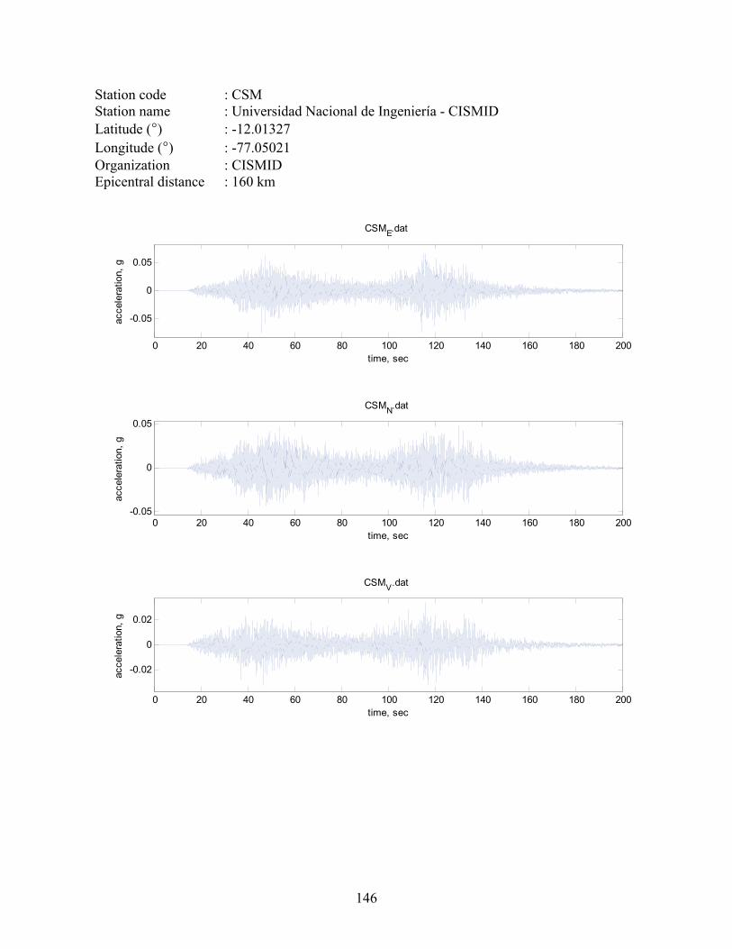
146
Station code : CSM Station name : Universidad Nacional de Ingeniería - CISMID Latitude (°) : -12.01327 Longitude (°) : -77.05021 Organization : CISMID Epicentral distance : 160 km
0 20 40 60 80 100 120 140 160 180 200
-0.05
0
0.05
time, sec
acce
lera
tion,
g
CSME.dat
0 20 40 60 80 100 120 140 160 180 200-0.05
0
0.05
time, sec
acce
lera
tion,
g
CSMN.dat
0 20 40 60 80 100 120 140 160 180 200
-0.02
0
0.02
time, sec
acce
lera
tion,
g
CSMV
.dat

147
0 0.5 1 1.5 2 2.5 30
0.05
0.1
0.15
0.2
0.25
Period, sec
Spe
ctra
l acc
eler
atio
n, g
CSME.dat
Elastic, =5%
Ductility=2, =2%
Ductility=4, =2%
0 0.5 1 1.5 2 2.5 30
0.05
0.1
0.15
0.2
0.25
Period, sec
Spe
ctra
l acc
eler
atio
n, g
CSMN.dat
Elastic, =5%
Ductility=2, =2%
Ductility=4, =2%
0 0.5 1 1.5 2 2.5 30
0.05
0.1
0.15
0.2
0.25
Period, sec
Spe
ctra
l acc
eler
atio
n, g
CSMV
.dat
Elastic, =5%
Ductility=2, =2%
Ductility=4, =2%
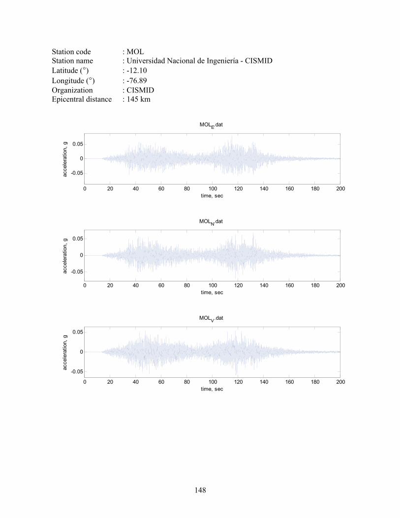
148
Station code : MOL Station name : Universidad Nacional de Ingeniería - CISMID Latitude (°) : -12.10 Longitude (°) : -76.89 Organization : CISMID Epicentral distance : 145 km
0 20 40 60 80 100 120 140 160 180 200
-0.05
0
0.05
time, sec
acce
lera
tion,
g
MOLE.dat
0 20 40 60 80 100 120 140 160 180 200
-0.05
0
0.05
time, sec
acce
lera
tion,
g
MOLN.dat
0 20 40 60 80 100 120 140 160 180 200
-0.05
0
0.05
time, sec
acce
lera
tion,
g
MOLV
.dat

149
0 0.5 1 1.5 2 2.5 30
0.05
0.1
0.15
0.2
0.25
0.3
0.35
0.4
Period, sec
Spe
ctra
l acc
eler
atio
n, g
MOLE.dat
Elastic, =5%
Ductility=2, =2%
Ductility=4, =2%
0 0.5 1 1.5 2 2.5 30
0.05
0.1
0.15
0.2
0.25
0.3
0.35
0.4
Period, sec
Spe
ctra
l acc
eler
atio
n, g
MOLN.dat
Elastic, =5%
Ductility=2, =2%
Ductility=4, =2%
0 0.5 1 1.5 2 2.5 30
0.05
0.1
0.15
0.2
0.25
0.3
0.35
0.4
Period, sec
Spe
ctra
l acc
eler
atio
n, g
MOLV
.dat
Elastic, =5%
Ductility=2, =2%
Ductility=4, =2%
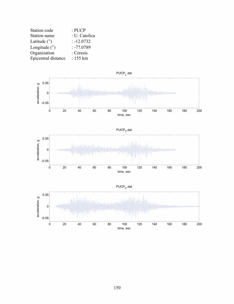
150
Station code : PUCP Station name : U. Catolica Latitude (°) : -12.0732 Longitude (°) : -77.0789 Organization : Ceresis Epicentral distance : 155 km
0 20 40 60 80 100 120 140 160 180 200
-0.05
0
0.05
time, sec
acce
lera
tion,
g
PUCPL.dat
0 20 40 60 80 100 120 140 160 180 200
-0.05
0
0.05
time, sec
acce
lera
tion,
g
PUCPT.dat
0 20 40 60 80 100 120 140 160 180 200
-0.05
0
0.05
time, sec
acce
lera
tion,
g
PUCPV
.dat

151
0 0.5 1 1.5 2 2.5 30
0.05
0.1
0.15
0.2
0.25
Period, sec
Spe
ctra
l acc
eler
atio
n, g
PUCPL.dat
Elastic, =5%
Ductility=2, =2%
Ductility=4, =2%
0 0.5 1 1.5 2 2.5 30
0.05
0.1
0.15
0.2
0.25
Period, sec
Spe
ctra
l acc
eler
atio
n, g
PUCPT.dat
Elastic, =5%
Ductility=2, =2%
Ductility=4, =2%
0 0.5 1 1.5 2 2.5 30
0.05
0.1
0.15
0.2
0.25
Period, sec
Spe
ctra
l acc
eler
atio
n, g
PUCPV
.dat
Elastic, =5%
Ductility=2, =2%
Ductility=4, =2%

152
Station code : RIN Station name : Rinconada Latitude (°) : N/A Longitude (°) : N/A Organization : Ceresis, IGP Epicentral distance : Approximately 150 km
0 20 40 60 80 100 120 140 160 180 200
-0.1
-0.05
0
0.05
0.1
time, sec
acce
lera
tion,
g
RINL.dat
0 20 40 60 80 100 120 140 160 180 200
-0.1
-0.05
0
0.05
0.1
time, sec
acce
lera
tion,
g
RINT.dat
0 20 40 60 80 100 120 140 160 180 200
-0.05
0
0.05
time, sec
acce
lera
tion,
g
RINV
.dat

153
0 0.5 1 1.5 2 2.5 30
0.1
0.2
0.3
0.4
0.5
Period, sec
Spe
ctra
l acc
eler
atio
n, g
RINL.dat
Elastic, =5%
Ductility=2, =2%
Ductility=4, =2%
0 0.5 1 1.5 2 2.5 30
0.1
0.2
0.3
0.4
0.5
Period, sec
Spe
ctra
l acc
eler
atio
n, g
RINT.dat
Elastic, =5%
Ductility=2, =2%
Ductility=4, =2%
0 0.5 1 1.5 2 2.5 30
0.1
0.2
0.3
0.4
0.5
Period, sec
Spe
ctra
l acc
eler
atio
n, g
RINV
.dat
Elastic, =5%
Ductility=2, =2%
Ductility=4, =2%

154
Station code : ANC Station name : Ancón Latitude (°) : -11.59 Longitude (°) : -76.15 Organization : IGP Epicentral distance : 200 km Comment : Digital forms of records are not released. Reference is made to IGP (2007) for original image.

155
Station code : MAY Station name : Mayorazgo Latitude (°) : -12.055 Longitude (°) : -76.944 Organization : IGP Epicentral distance : 152 km Comment : Digital forms of records are not released. Reference is made to IGP (2007) for original image.
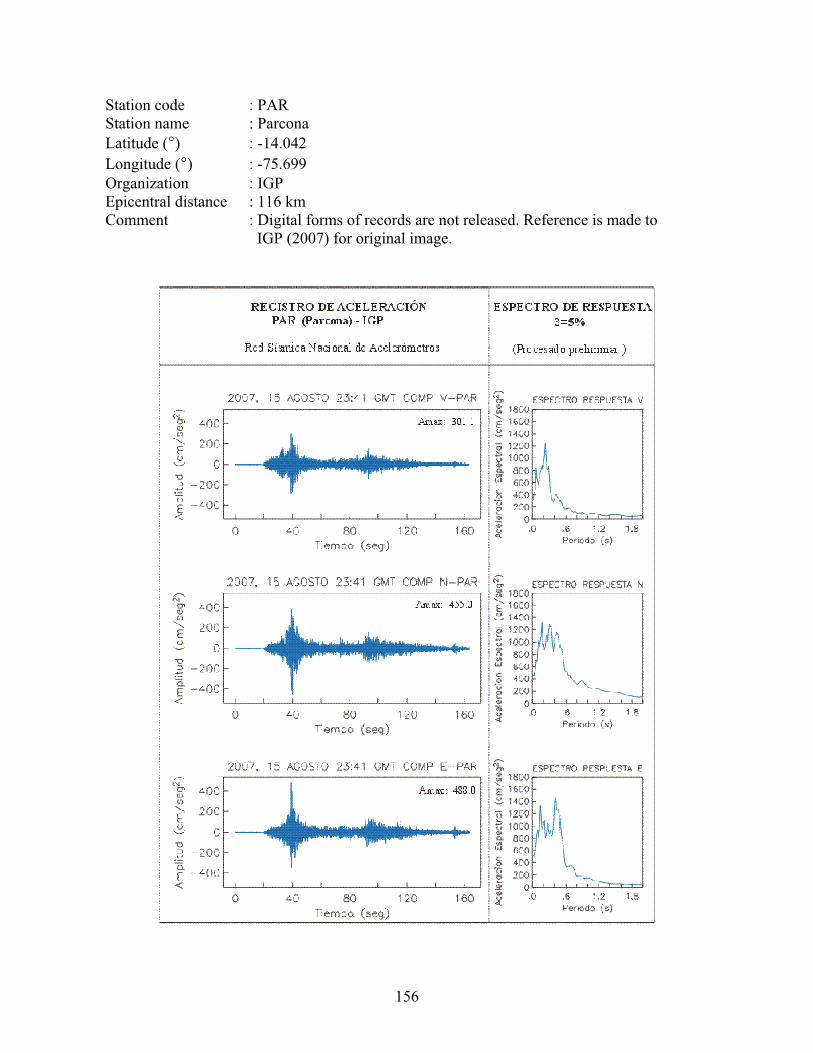
156
Station code : PAR Station name : Parcona Latitude (°) : -14.042 Longitude (°) : -75.699 Organization : IGP Epicentral distance : 116 km Comment : Digital forms of records are not released. Reference is made to IGP (2007) for original image.

The coastal region of Central Peru was hit by a major offshore earthquake of magnitude 8.0 ±0.1 on 15 August 2007; the event is hereafter referred to as the Pisco-Chincha earthquake. TheMid-America Earthquake Center dispatched a field reconnaissance team to the affected areal th t k l t Th MAE C t t j i d b t f U i id dless than two weeks later. The MAE Center team was joined by experts from UniversidadNacional de Ingeniería and Centro Peruano-Japonés de Investigaciones Sísmicas y Mitigaciónde Desastres. The combined team spent one week in the field, followed by many months ofback-analysis and detailed investigation of the collected information. This report summarizesthe work of the team on the historical earthquake catalogue of Peru, and the attribution ofeach major earthquake to the complex and multiple inclinations subduction regimecontrolling the seismicity of the coastal Peruvian planes. It includes an in-depth study of theattenuation of ground motion and application of a modern and well-verified strong-motionmodel to the derivation of hazard maps for the region. The available acceleration records areextensively analyzed and elastic and inelastic spectra derived, and compared to earthquakesof similar magnitude. A set of records are selected from the international data bank torepresent the hazard from the Pisco-Chincha earthquakes in regions where no records areavailable. Significant effort is allocated in the report to the geological and geotechnicalsettings as well as observations of damage to foundation, slumping and soil liquefaction. Astructure in the university of Ica complex that was damaged by the earthquake is modeledand back-analyzed using an actual record from the Pisco-Chincha earthquake. The failuremode is identified and attributed to layout and design deficiencies. Comments on thestructural performance of all types of buildings and bridges are made. The report concludeswith a summary of the findings, and recommendations covering hazard, risk management,design and construction, and legislation.
The Mid-America Earthquake Center is a National Science Foundation Engineering ResearchCenter, funded under cooperative agreement reference EEC 97-01785
Director: Amr S. ElnashaiManaging Director: Timothy A. Gress


![Final Pisco Peru Grupo 5[2]](https://static.fdocuments.us/doc/165x107/577d24dc1a28ab4e1e9d94d1/final-pisco-peru-grupo-52.jpg)