Repeated Measures ANOVA - Stony Brookzhu/ams394/RepeatedMeasuresANOVA.pdf · The One-way ANOVA we...
90
Repeated Measures ANOVA Prof. Wei Zhu Department of Applied Mathematics & Statistics Stony Brook University
-
Upload
duongkhuong -
Category
Documents
-
view
236 -
download
0
Transcript of Repeated Measures ANOVA - Stony Brookzhu/ams394/RepeatedMeasuresANOVA.pdf · The One-way ANOVA we...

Repeated Measures ANOVA
Prof. Wei Zhu
Department of Applied Mathematics & Statistics
Stony Brook University
2
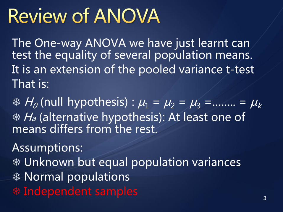
The One-way ANOVA we have just learnt can test the equality of several population means. It is an extension of the pooled variance t-test That is:
H0 (null hypothesis) : µ1 = µ2 = µ3 =…….. = µk
Ha (alternative hypothesis): At least one of means differs from the rest.
Assumptions: Unknown but equal population variances Normal populations Independent samples
3
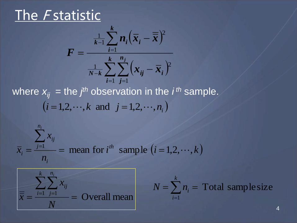
The F statistic
k
i
n
j
iijkN
k
i
iik
j
xx
xxn
F
1 1
21
1
2
11
where xij = the jth observation in the i th sample.
injki ,,2,1 and ,,2,1
kiin
x
x th
i
n
j
ij
i
i
,,2,1 sample for mean 1
size sample Total 1
k
i
inNmean Overall
1 1
N
x
x
k
i
n
j
ij
i
4
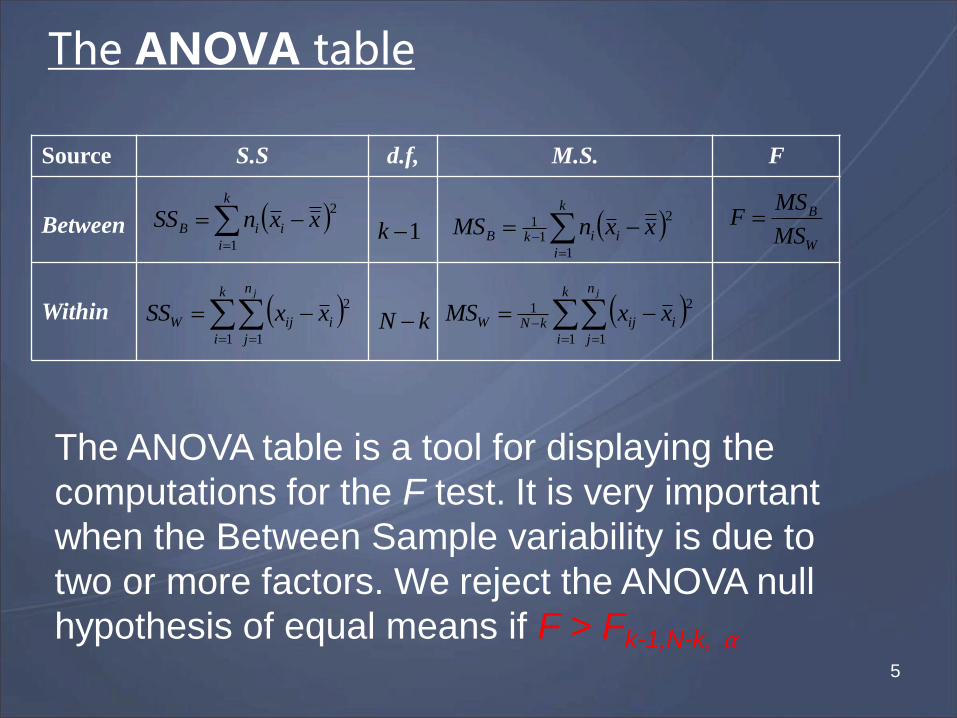
The ANOVA table
k
i
iiB xxnSS1
2
W
B
MS
MSF
k
i
iikB xxnMS1
2
11
k
i
n
j
iijW
j
xxSS1 1
2
k
i
n
j
iijkNW
j
xxMS1 1
21
1k
kN
Source S.S d.f, M.S. F
Between
Within
The ANOVA table is a tool for displaying the
computations for the F test. It is very important
when the Between Sample variability is due to
two or more factors. We reject the ANOVA null
hypothesis of equal means if F > Fk-1,N-k, α
5
The most distinct disadvantage to the analysis of variance (ANOVA) method is that it requires three assumptions to be made:
☼ The samples must be independent to each other.
☼ All variances from each data group, though unknown, must be equal.The normality assumption.
Limitations of the one-way ANOVA:
6

7
☼ A repeated measures design is one in which at least one of the factors consists of repeated measurements on the same subjects or experimental units, under different conditions and/or at different time points.
8
A repeated measures design often involves measuring subjects at different points in time – or subjects measured under different experimental conditions
It can be viewed as an extension of the paired-samples t-test (which involved only two related measures)
Thus, the measures—unlike in the “regular” ANOVA—are correlated, that is, the observations are not independent
9
Example: Data collected in a sequence of (often) evenly spaced points in time – this is usually referred to as the ‘longitudinal data’
Example: Different treatments are assigned to the each experimental unit
10
By collecting data from the same participants under repeated conditions, the individual differences can be eliminated or reduced as a source of between group differences.
Also, the sample size is not divided between conditions or groups and thus inferential testing becomes more powerful.
This design also proves to be economical when sample members are difficult to recruit.
11
12
As with any ANOVA, repeated measures ANOVA tests
the equality of means. However, repeated measures
ANOVA is used when all members of a random sample
are measured under a number of different conditions or
at different time points.
As the sample is exposed to each condition, the
measurement of the dependent variable is repeated.
Using a standard ANOVA in this case is not
appropriate because it fails to model the correlation
between the repeated measures: the data violate the
ANOVA assumption of independence. 13
The simplest example of a repeated measures design is a paired samples t-test: Each subject is measured twice, for example, time 1 and time 2, on the same variable; or, each pair of matched participants are assigned to two treatment levels. If we observe participants at more than two time-points, then we need to conduct a repeated measures ANOVA.
14
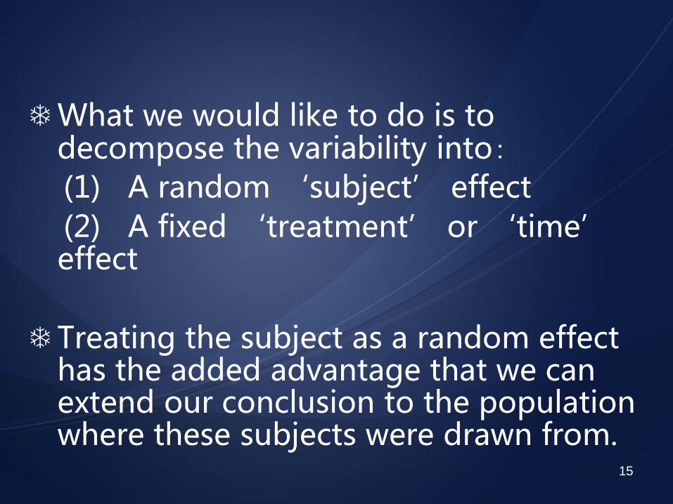
What we would like to do is to decompose the variability into:
(1) A random ‘subject’ effect (2) A fixed ‘treatment’ or ‘time’
effect Treating the subject as a random effect
has the added advantage that we can extend our conclusion to the population where these subjects were drawn from.
15
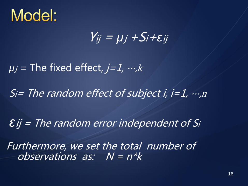
Yij = μ j +Si+εij μ j = The fixed effect, j=1, ⋯,k Si= The random effect of subject i, i=1, ⋯,n
εij = The random error independent of Si
Furthermore, we set the total number of observations as: N = n*k
16
17 17
18
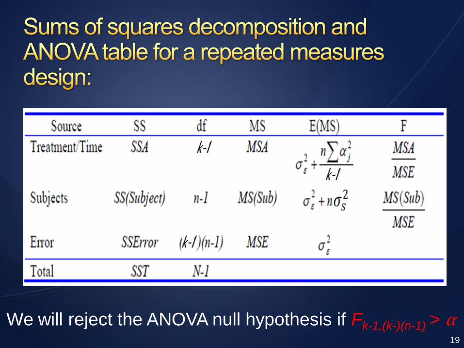
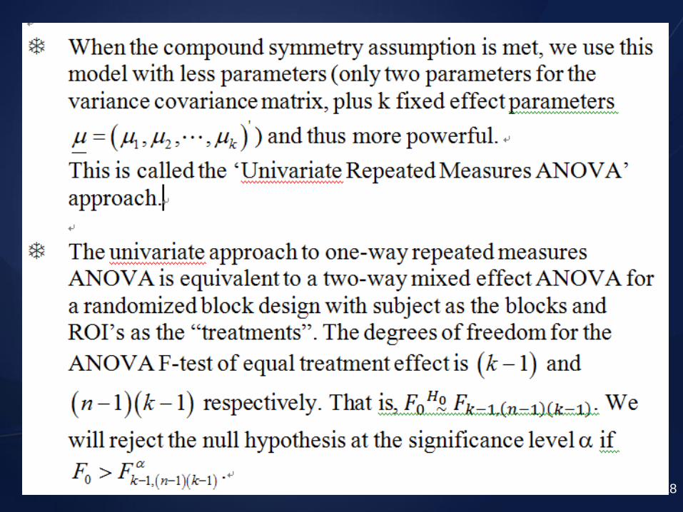
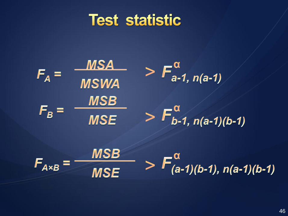
We will reject the ANOVA null hypothesis if Fk-1,(k-)(n-1) > α 19
20
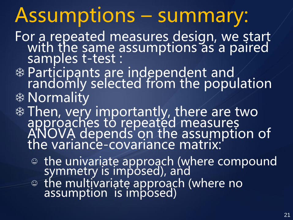
Assumptions – summary:
For a repeated measures design, we start with the same assumptions as a paired samples t-test :
Participants are independent and randomly selected from the population
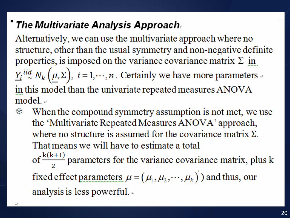
Normality Then, very importantly, there are two
approaches to repeated measures ANOVA depends on the assumption of the variance-covariance matrix:
☺ the univariate approach (where compound symmetry is imposed), and
☺ the multivariate approach (where no assumption is imposed)
21
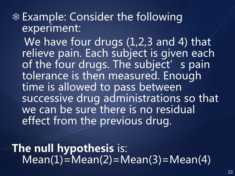
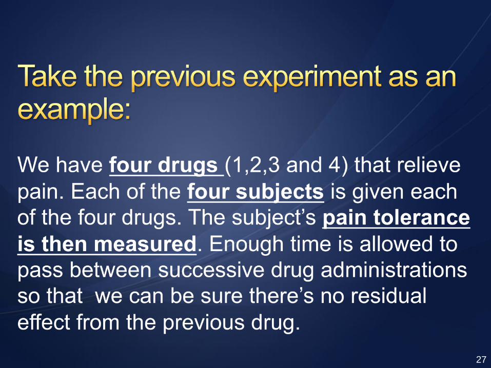
Example: Consider the following experiment:
We have four drugs (1,2,3 and 4) that relieve pain. Each subject is given each of the four drugs. The subject’s pain tolerance is then measured. Enough time is allowed to pass between successive drug administrations so that we can be sure there is no residual effect from the previous drug.
The null hypothesis is:
Mean(1)=Mean(2)=Mean(3)=Mean(4) 22
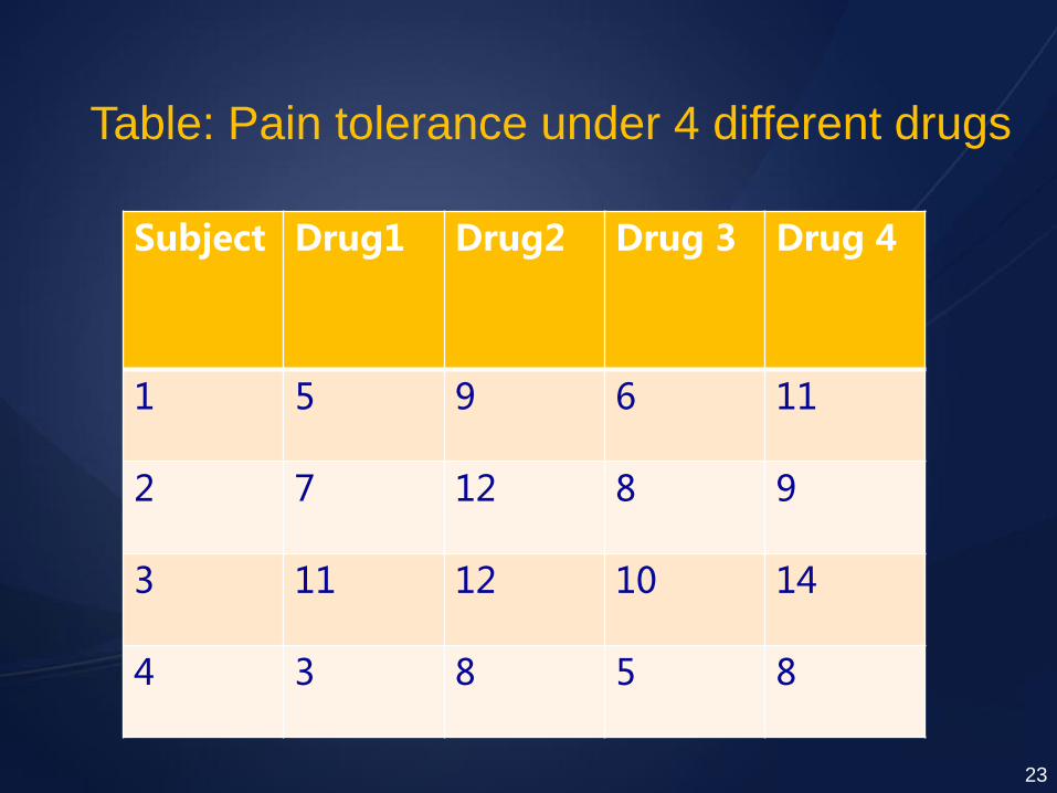
Subject Drug1 Drug2 Drug 3 Drug 4
1 5 9 6 11
2 7 12 8 9
3 11 12 10 14
4 3 8 5 8
Table: Pain tolerance under 4 different drugs
23
In the one-way analysis of variance without a repeated measure, we would have each subject receive only one of the four drugs. In this design, each subjects is measured under each of the drug conditions. This has several important advantages as enumerated before.
24
Each subject acts as his own control. i.e. : drugs effects are calculated by recording deviations between each drug score and the average drug score for each subject.
The normal subject-to-subject variation can thus be removed from the error sum of squares.
25
26
27
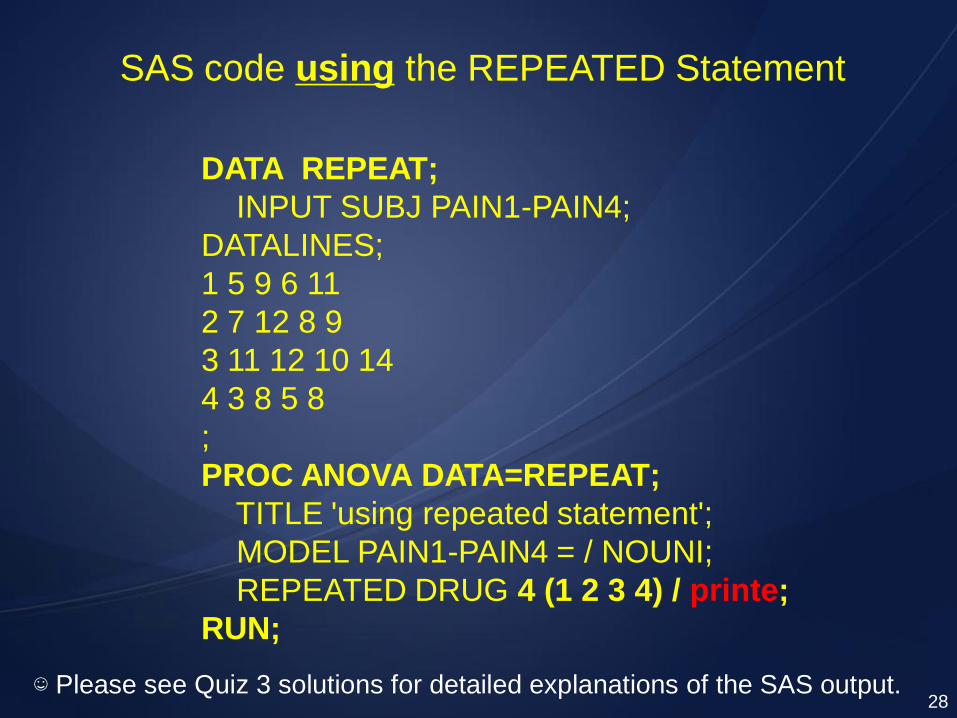
SAS code using the REPEATED Statement
DATA REPEAT;
INPUT SUBJ PAIN1-PAIN4;
DATALINES;
1 5 9 6 11
2 7 12 8 9
3 11 12 10 14
4 3 8 5 8
;
PROC ANOVA DATA=REPEAT;
TITLE 'using repeated statement';
MODEL PAIN1-PAIN4 = / NOUNI;
REPEATED DRUG 4 (1 2 3 4) / printe;
RUN;
28 ☺ Please see Quiz 3 solutions for detailed explanations of the SAS output.
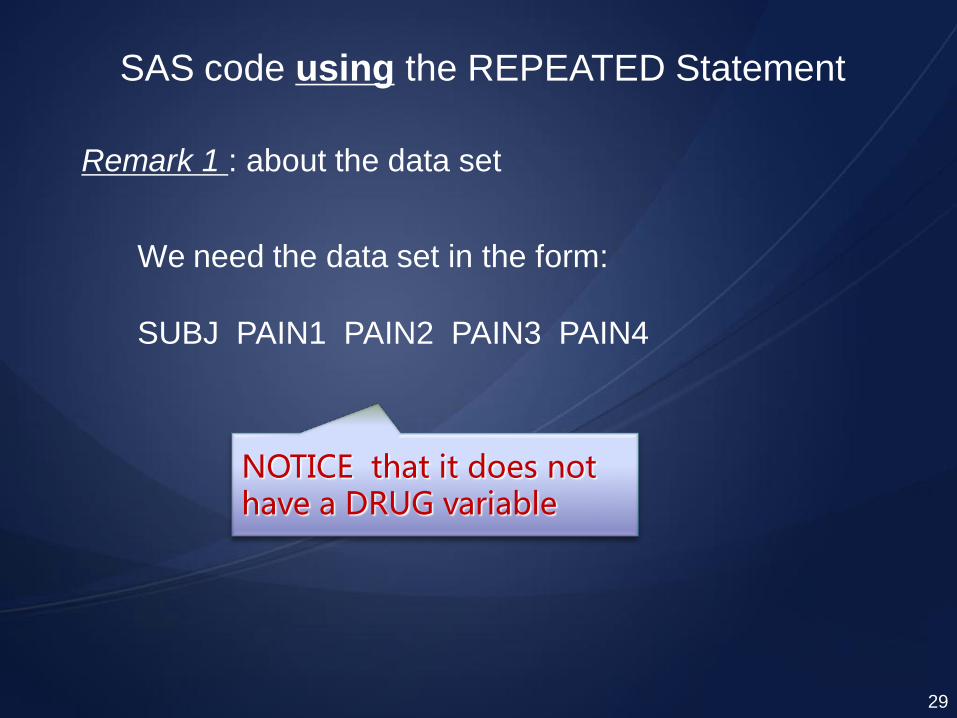
SAS code using the REPEATED Statement
Remark 1 : about the data set
We need the data set in the form:
SUBJ PAIN1 PAIN2 PAIN3 PAIN4
NOTICE that it does not have a DRUG variable
29
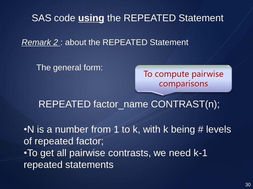
SAS code using the REPEATED Statement
Remark 2 : about the REPEATED Statement
The general form:
REPEATED factor_name CONTRAST(n);
To compute pairwise comparisons
•N is a number from 1 to k, with k being # levels
of repeated factor;
•To get all pairwise contrasts, we need k-1
repeated statements
30
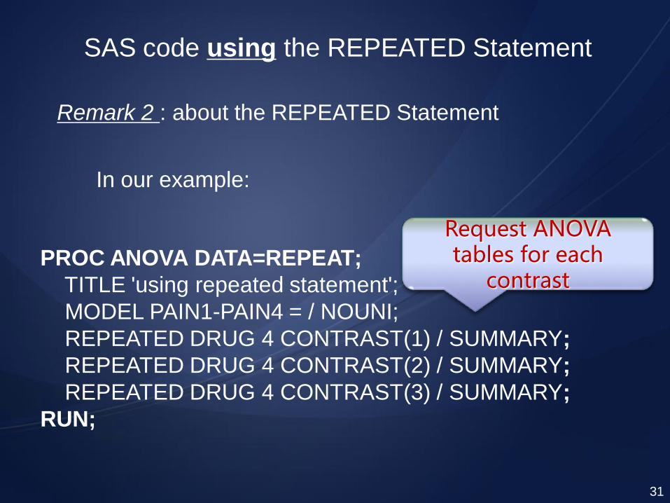
SAS code using the REPEATED Statement
Remark 2 : about the REPEATED Statement
In our example:
PROC ANOVA DATA=REPEAT;
TITLE 'using repeated statement';
MODEL PAIN1-PAIN4 = / NOUNI;
REPEATED DRUG 4 CONTRAST(1) / SUMMARY;
REPEATED DRUG 4 CONTRAST(2) / SUMMARY;
REPEATED DRUG 4 CONTRAST(3) / SUMMARY;
RUN;
Request ANOVA tables for each
contrast
31
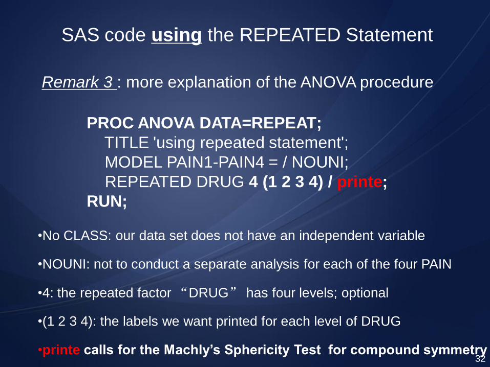
SAS code using the REPEATED Statement
Remark 3 : more explanation of the ANOVA procedure
PROC ANOVA DATA=REPEAT;
TITLE 'using repeated statement';
MODEL PAIN1-PAIN4 = / NOUNI;
REPEATED DRUG 4 (1 2 3 4) / printe;
RUN;
•No CLASS: our data set does not have an independent variable
•NOUNI: not to conduct a separate analysis for each of the four PAIN
•4: the repeated factor “DRUG” has four levels; optional
•(1 2 3 4): the labels we want printed for each level of DRUG
•printe calls for the Machly’s Sphericity Test for compound symmetry 32
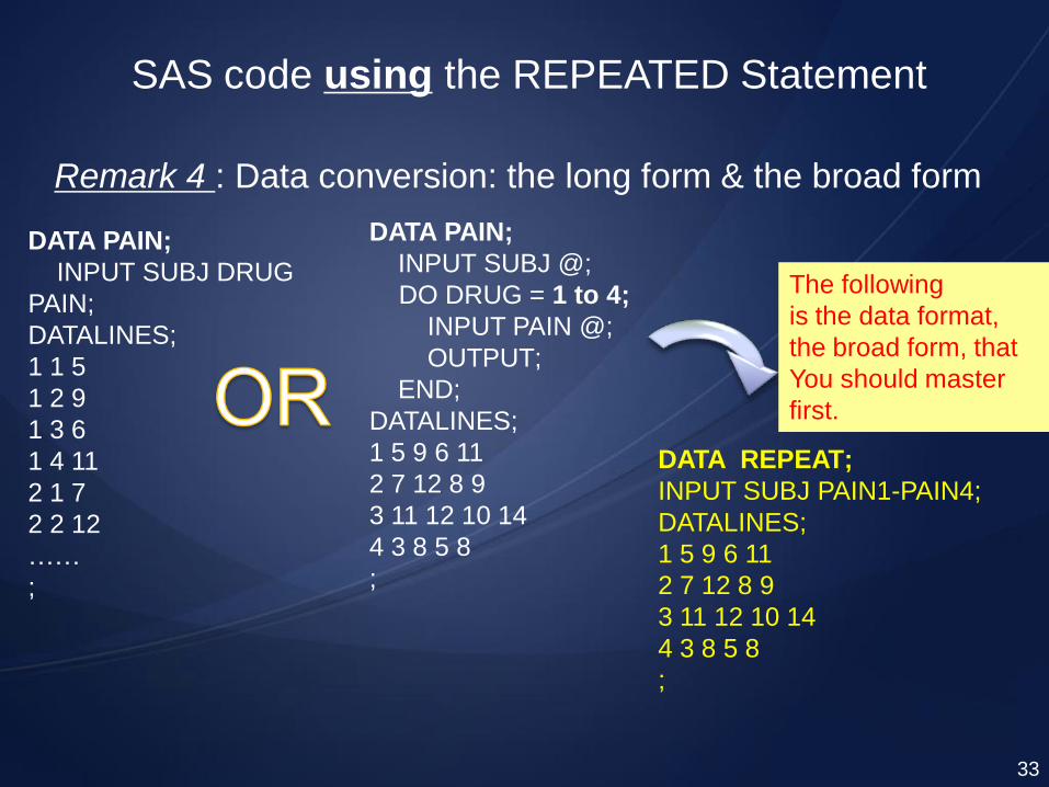
SAS code using the REPEATED Statement
Remark 4 : Data conversion: the long form & the broad form
DATA PAIN;
INPUT SUBJ DRUG
PAIN;
DATALINES;
1 1 5
1 2 9
1 3 6
1 4 11
2 1 7
2 2 12
……
;
DATA PAIN;
INPUT SUBJ @;
DO DRUG = 1 to 4;
INPUT PAIN @;
OUTPUT;
END;
DATALINES;
1 5 9 6 11
2 7 12 8 9
3 11 12 10 14
4 3 8 5 8
;
DATA REPEAT;
INPUT SUBJ PAIN1-PAIN4;
DATALINES;
1 5 9 6 11
2 7 12 8 9
3 11 12 10 14
4 3 8 5 8
;
The following
is the data format,
the broad form, that
You should master
first.
33
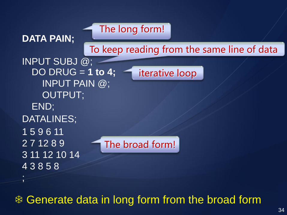
Generate data in long form from the broad form
DATA PAIN;
INPUT SUBJ @;
DATALINES;
DO DRUG = 1 to 4;
INPUT PAIN @;
OUTPUT;
END;
iterative loop
To keep reading from the same line of data
1 5 9 6 11
2 7 12 8 9
3 11 12 10 14
4 3 8 5 8
;
The broad form!
The long form!
34
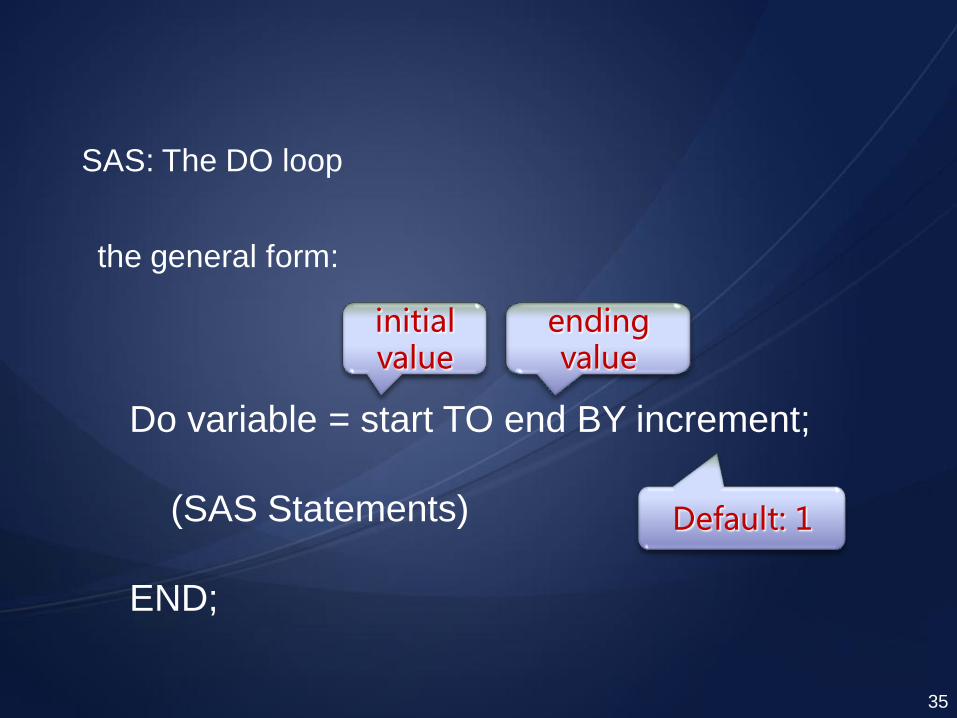
SAS: The DO loop
the general form:
Do variable = start TO end BY increment;
(SAS Statements)
END;
initial value
ending value
Default: 1
35
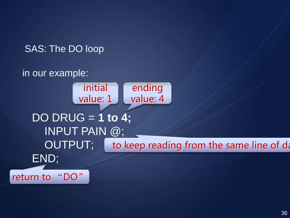
in our example:
initial value: 1
ending value: 4
DO DRUG = 1 to 4;
INPUT PAIN @;
OUTPUT;
END;
to keep reading from the same line of data
return to “DO”
SAS: The DO loop
36
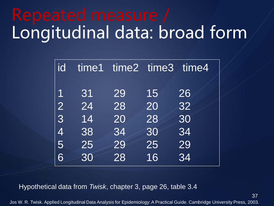
Repeated measure / Longitudinal data: broad form
37
id time1 time2 time3 time4
1 31 29 15 26
2 24 28 20 32
3 14 20 28 30
4 38 34 30 34
5 25 29 25 29
6 30 28 16 34
Hypothetical data from Twisk, chapter 3, page 26, table 3.4
Jos W. R. Twisk. Applied Longitudinal Data Analysis for Epidemiology: A Practical Guide. Cambridge University Press, 2003.
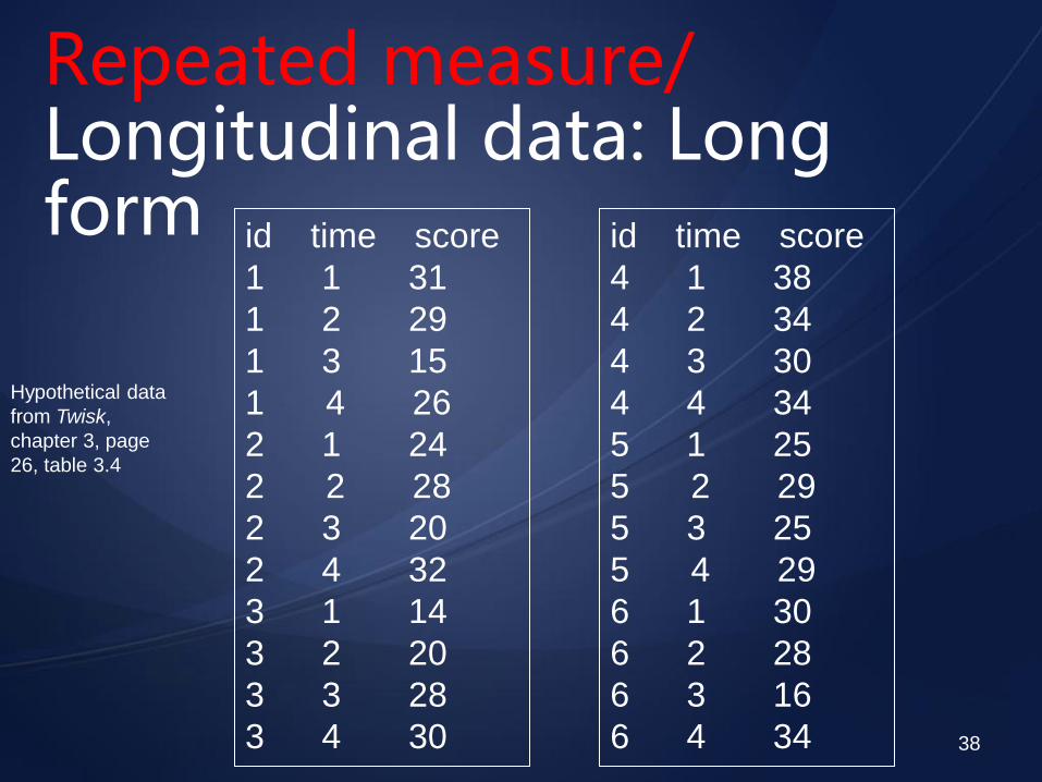
Repeated measure/ Longitudinal data: Long form
38
Hypothetical data
from Twisk,
chapter 3, page
26, table 3.4
id time score
1 1 31
1 2 29
1 3 15
1 4 26
2 1 24
2 2 28
2 3 20
2 4 32
3 1 14
3 2 20
3 3 28
3 4 30
id time score
4 1 38
4 2 34
4 3 30
4 4 34
5 1 25
5 2 29
5 3 25
5 4 29
6 1 30
6 2 28
6 3 16
6 4 34
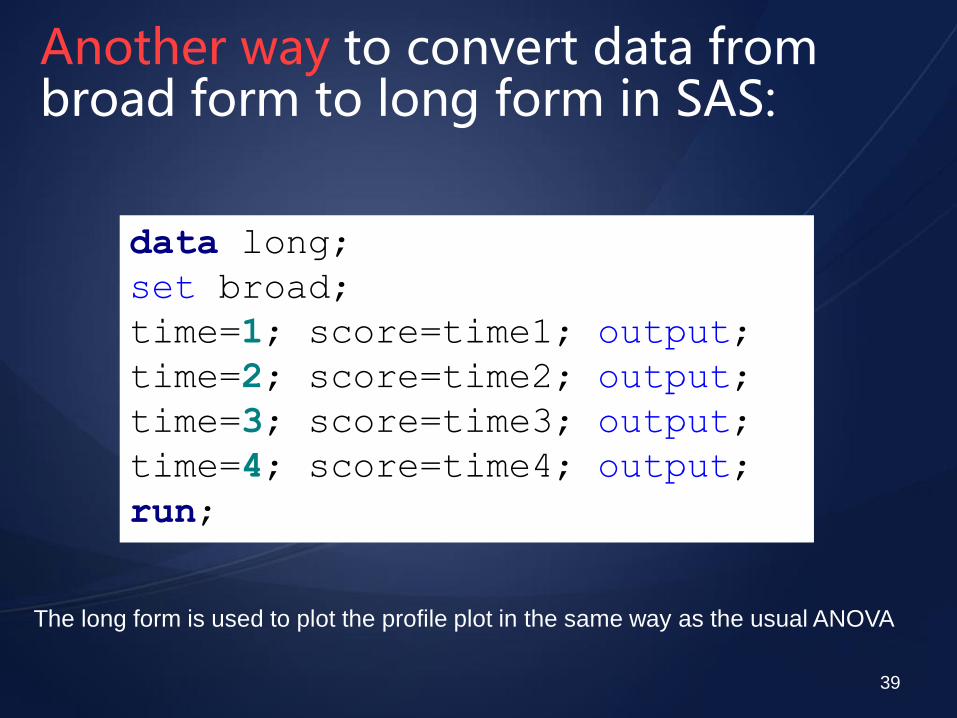
Another way to convert data from broad form to long form in SAS:
39
data long;
set broad;
time=1; score=time1; output;
time=2; score=time2; output;
time=3; score=time3; output;
time=4; score=time4; output;
run;
The long form is used to plot the profile plot in the same way as the usual ANOVA

40
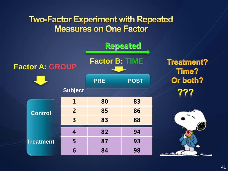
1 80 83
2 85 86
3 83 88
4 82 94
5 87 93
6 84 98
Subject
Control
Treatment
PRE POST
Factor B: TIME Factor A: GROUP
Repeated
41
42
43
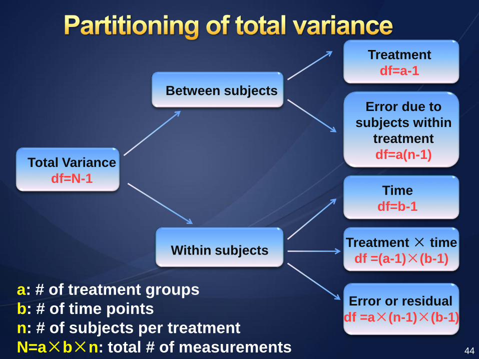
Total Variance
df=N-1
Between subjects
Within subjects
Treatment
df=a-1
Error due to
subjects within
treatment
df=a(n-1)
Time
df=b-1
Treatment × time
df =(a-1)×(b-1)
Error or residual
df =a×(n-1)×(b-1)
a: # of treatment groups
b: # of time points
n: # of subjects per treatment
N=a×b×n: total # of measurements 44
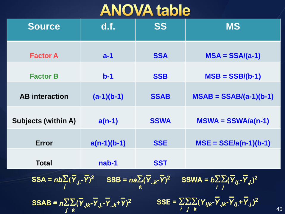
Source d.f. SS MS
Factor A
a-1
SSA
MSA = SSA/(a-1)
Factor B
b-1
SSB
MSB = SSB/(b-1)
AB interaction
(a-1)(b-1)
SSAB
MSAB = SSAB/(a-1)(b-1)
Subjects (within A)
a(n-1)
SSWA
MSWA = SSWA/a(n-1)
Error
a(n-1)(b-1)
SSE
MSE = SSE/a(n-1)(b-1)
Total
nab-1
SST
45
46
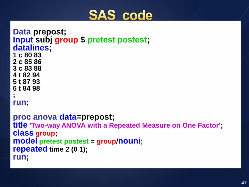
Data prepost; Input subj group $ pretest postest; datalines; 1 c 80 83 2 c 85 86 3 c 83 88 4 t 82 94 5 t 87 93 6 t 84 98 ; run; proc anova data=prepost; title 'Two-way ANOVA with a Repeated Measure on One Factor'; class group; model pretest postest = group/nouni; repeated time 2 (0 1); run;
47
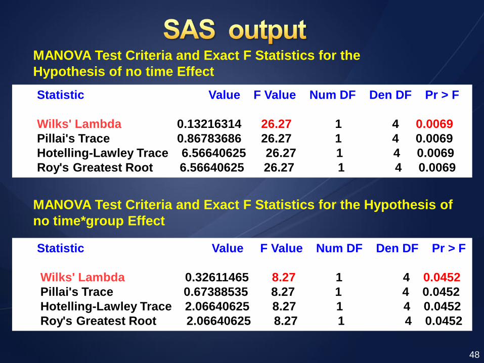
Statistic Value F Value Num DF Den DF Pr > F
Wilks' Lambda 0.13216314 26.27 1 4 0.0069
Pillai's Trace 0.86783686 26.27 1 4 0.0069
Hotelling-Lawley Trace 6.56640625 26.27 1 4 0.0069
Roy's Greatest Root 6.56640625 26.27 1 4 0.0069
MANOVA Test Criteria and Exact F Statistics for the
Hypothesis of no time Effect
MANOVA Test Criteria and Exact F Statistics for the Hypothesis of
no time*group Effect
Statistic Value F Value Num DF Den DF Pr > F
Wilks' Lambda 0.32611465 8.27 1 4 0.0452
Pillai's Trace 0.67388535 8.27 1 4 0.0452
Hotelling-Lawley Trace 2.06640625 8.27 1 4 0.0452
Roy's Greatest Root 2.06640625 8.27 1 4 0.0452
48
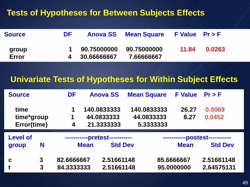
Tests of Hypotheses for Between Subjects Effects
Source DF Anova SS Mean Square F Value Pr > F
group 1 90.75000000 90.75000000 11.84 0.0263
Error 4 30.66666667 7.66666667
Univariate Tests of Hypotheses for Within Subject Effects
Source DF Anova SS Mean Square F Value Pr > F
time 1 140.0833333 140.0833333 26.27 0.0069
time*group 1 44.0833333 44.0833333 8.27 0.0452
Error(time) 4 21.3333333 5.3333333
Level of -----------pretest----------- -----------postest-----------
group N Mean Std Dev Mean Std Dev
c 3 82.6666667 2.51661148 85.6666667 2.51661148
t 3 84.3333333 2.51661148 95.0000000 2.64575131
49
Another Example
50
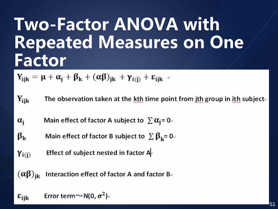
Two-Factor ANOVA with Repeated Measures on One Factor
51
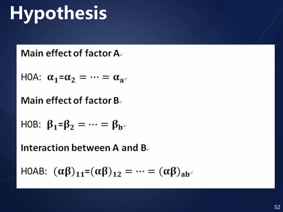
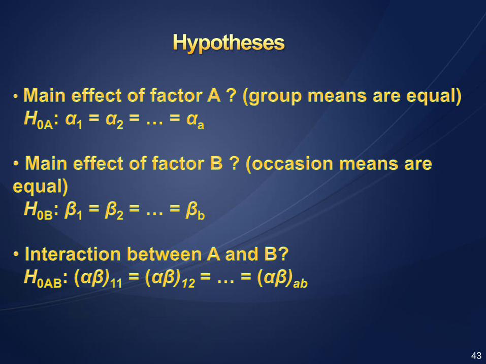
Hypothesis
52
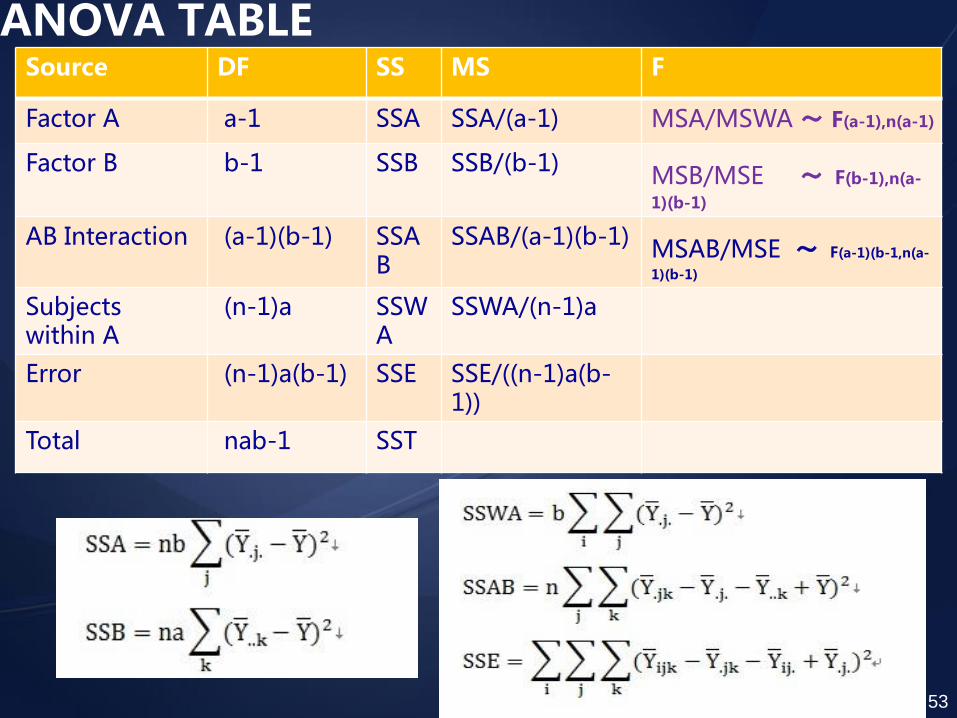
ANOVA TABLE Source DF SS MS F
Factor A a-1 SSA SSA/(a-1) MSA/MSWA ~ F(a-1),n(a-1)
Factor B b-1 SSB SSB/(b-1) MSB/MSE ~ F(b-1),n(a-
1)(b-1)
AB Interaction (a-1)(b-1) SSAB
SSAB/(a-1)(b-1) MSAB/MSE ~ F(a-1)(b-1,n(a-
1)(b-1)
Subjects within A
(n-1)a SSWA
SSWA/(n-1)a
Error (n-1)a(b-1) SSE SSE/((n-1)a(b-1))
Total nab-1 SST
53
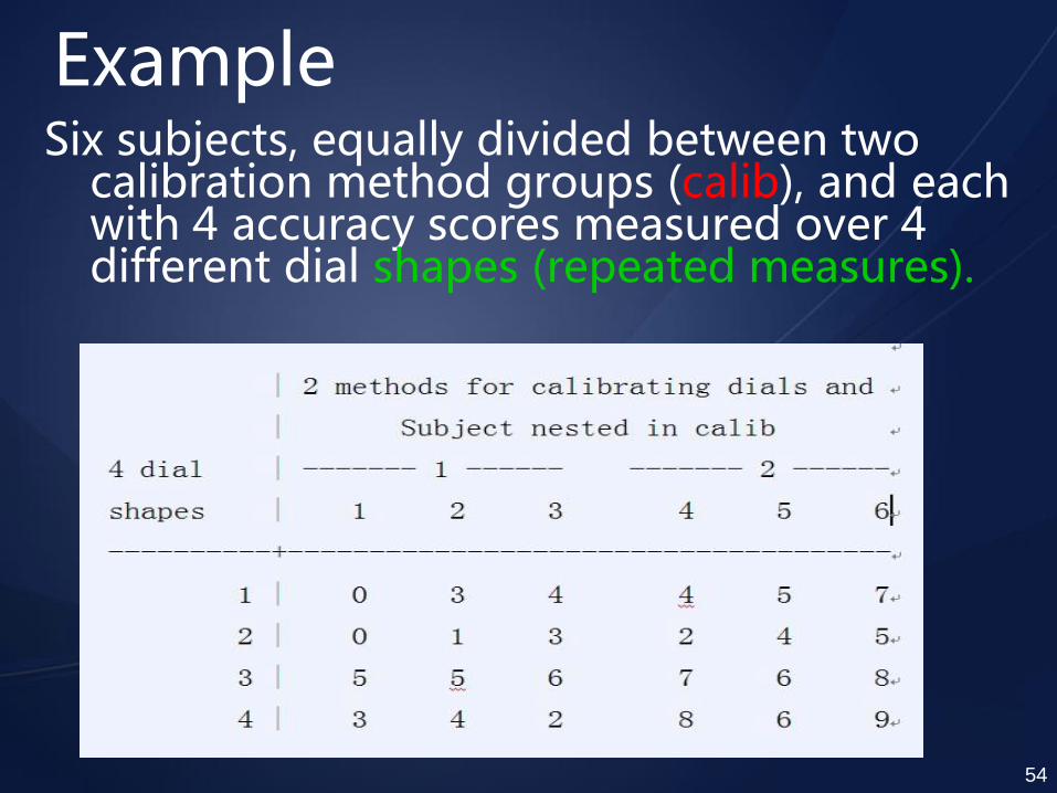
Example Six subjects, equally divided between two
calibration method groups (calib), and each with 4 accuracy scores measured over 4 different dial shapes (repeated measures).
54
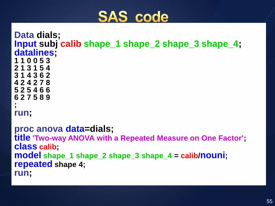
Data dials; Input subj calib shape_1 shape_2 shape_3 shape_4; datalines; 1 1 0 0 5 3 2 1 3 1 5 4 3 1 4 3 6 2 4 2 4 2 7 8 5 2 5 4 6 6 6 2 7 5 8 9 ; run; proc anova data=dials; title 'Two-way ANOVA with a Repeated Measure on One Factor'; class calib; model shape_1 shape_2 shape_3 shape_4 = calib/nouni; repeated shape 4; run;
55
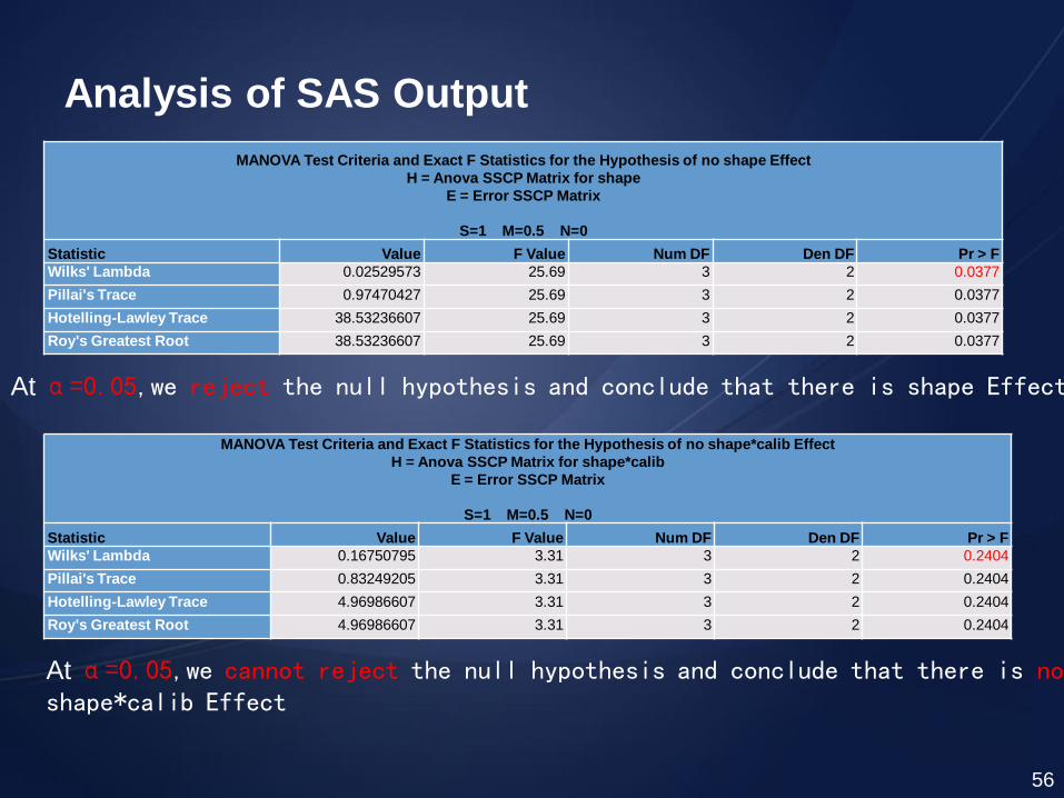
MANOVA Test Criteria and Exact F Statistics for the Hypothesis of no shape Effect
H = Anova SSCP Matrix for shape
E = Error SSCP Matrix
S=1 M=0.5 N=0
Statistic Value F Value Num DF Den DF Pr > F
Wilks' Lambda 0.02529573 25.69 3 2 0.0377
Pillai's Trace 0.97470427 25.69 3 2 0.0377
Hotelling-Lawley Trace 38.53236607 25.69 3 2 0.0377
Roy's Greatest Root 38.53236607 25.69 3 2 0.0377
MANOVA Test Criteria and Exact F Statistics for the Hypothesis of no shape*calib Effect
H = Anova SSCP Matrix for shape*calib
E = Error SSCP Matrix
S=1 M=0.5 N=0
Statistic Value F Value Num DF Den DF Pr > F
Wilks' Lambda 0.16750795 3.31 3 2 0.2404
Pillai's Trace 0.83249205 3.31 3 2 0.2404
Hotelling-Lawley Trace 4.96986607 3.31 3 2 0.2404
Roy's Greatest Root 4.96986607 3.31 3 2 0.2404
At α=0.05,we reject the null hypothesis and conclude that there is shape Effect
At α=0.05,we cannot reject the null hypothesis and conclude that there is no shape*calib Effect
Analysis of SAS Output
56
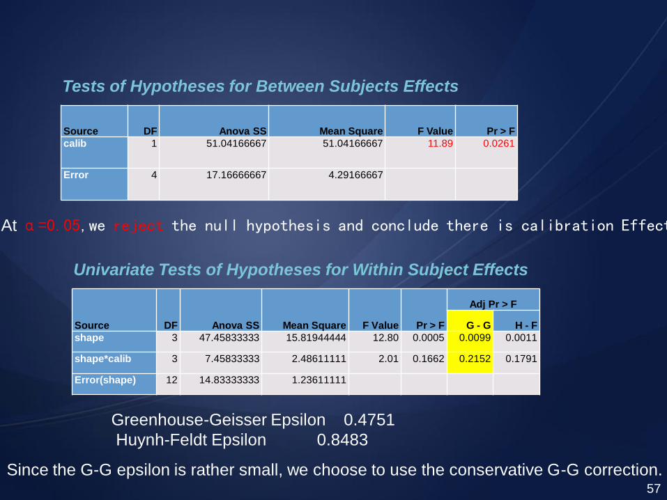
Source DF Anova SS Mean Square F Value Pr > F
calib 1 51.04166667 51.04166667 11.89 0.0261
Error 4 17.16666667 4.29166667
Source DF Anova SS Mean Square F Value Pr > F
Adj Pr > F
G - G H - F
shape 3 47.45833333 15.81944444 12.80 0.0005 0.0099 0.0011
shape*calib 3 7.45833333 2.48611111 2.01 0.1662 0.2152 0.1791
Error(shape) 12 14.83333333 1.23611111
Univariate Tests of Hypotheses for Within Subject Effects
Tests of Hypotheses for Between Subjects Effects
57
At α=0.05,we reject the null hypothesis and conclude there is calibration Effect
Greenhouse-Geisser Epsilon 0.4751
Huynh-Feldt Epsilon 0.8483
Since the G-G epsilon is rather small, we choose to use the conservative G-G correction.
58
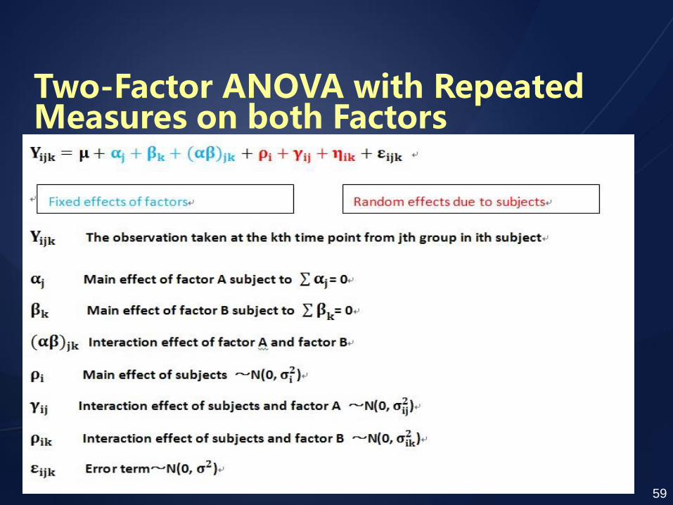
Two-Factor ANOVA with Repeated Measures on both Factors
59
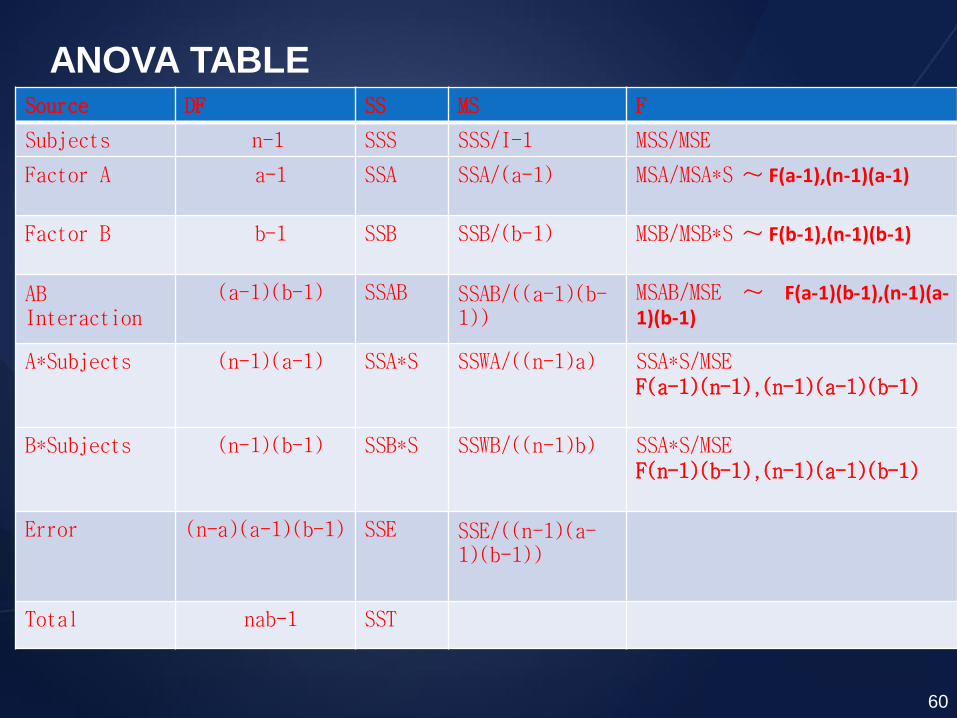
Source DF SS MS F
Subjects n-1 SSS SSS/I-1 MSS/MSE
Factor A a-1 SSA SSA/(a-1) MSA/MSA*S ~ F(a-1),(n-1)(a-1)
Factor B b-1 SSB SSB/(b-1) MSB/MSB*S ~ F(b-1),(n-1)(b-1)
AB Interaction
(a-1)(b-1) SSAB SSAB/((a-1)(b-1))
MSAB/MSE ~ F(a-1)(b-1),(n-1)(a-1)(b-1)
A*Subjects (n-1)(a-1) SSA*S SSWA/((n-1)a) SSA*S/MSE F(a-1)(n-1),(n-1)(a-1)(b-1)
B*Subjects (n-1)(b-1) SSB*S SSWB/((n-1)b) SSA*S/MSE F(n-1)(b-1),(n-1)(a-1)(b-1)
Error (n-a)(a-1)(b-1) SSE SSE/((n-1)(a-1)(b-1))
Total nab-1 SST
ANOVA TABLE
60
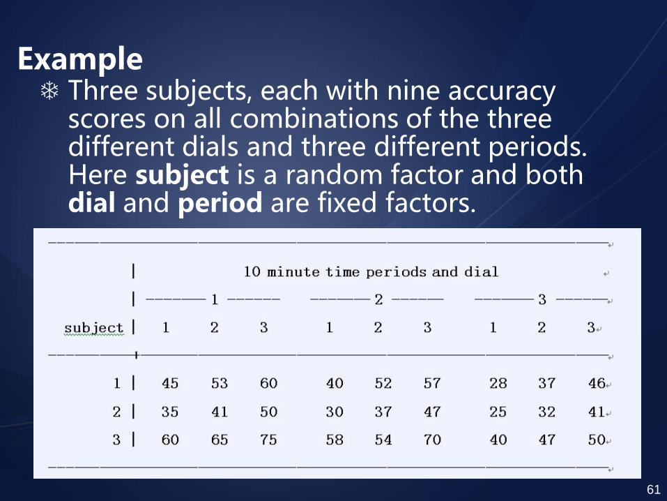
Example Three subjects, each with nine accuracy
scores on all combinations of the three different dials and three different periods. Here subject is a random factor and both dial and period are fixed factors.
61
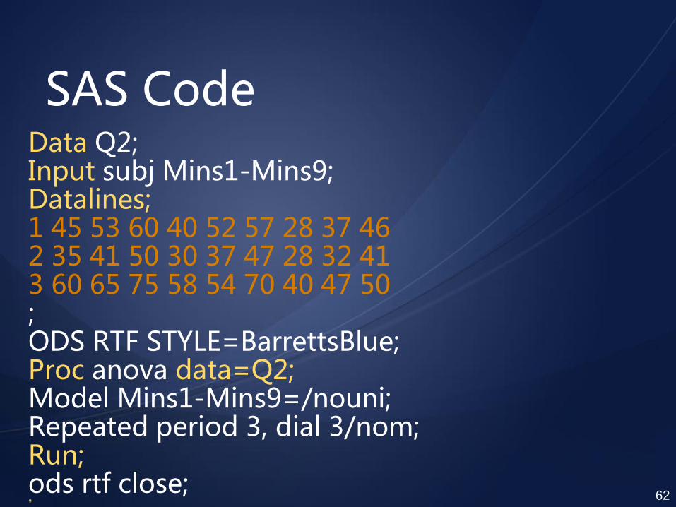
SAS Code Data Q2; Input subj Mins1-Mins9; Datalines; 1 45 53 60 40 52 57 28 37 46 2 35 41 50 30 37 47 28 32 41 3 60 65 75 58 54 70 40 47 50 ; ODS RTF STYLE=BarrettsBlue; Proc anova data=Q2; Model Mins1-Mins9=/nouni; Repeated period 3, dial 3/nom; Run; ods rtf close;
62
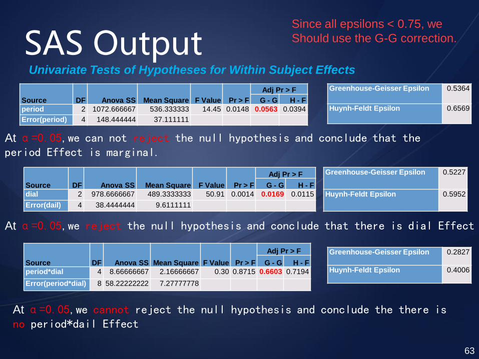
SAS Output
Source DF Anova SS Mean Square F Value Pr > F
Adj Pr > F
G - G H - F
period 2 1072.666667 536.333333 14.45 0.0148 0.0563 0.0394
Error(period) 4 148.444444 37.111111
Greenhouse-Geisser Epsilon 0.5364
Huynh-Feldt Epsilon 0.6569
Source DF Anova SS Mean Square F Value Pr > F
Adj Pr > F
G - G H - F
dial 2 978.6666667 489.3333333 50.91 0.0014 0.0169 0.0115
Error(dail) 4 38.4444444 9.6111111
Greenhouse-Geisser Epsilon 0.5227
Huynh-Feldt Epsilon 0.5952
Source DF Anova SS Mean Square F Value Pr > F
Adj Pr > F
G - G H - F
period*dial 4 8.66666667 2.16666667 0.30 0.8715 0.6603 0.7194
Error(period*dial) 8 58.22222222 7.27777778
Greenhouse-Geisser Epsilon 0.2827
Huynh-Feldt Epsilon 0.4006
Univariate Tests of Hypotheses for Within Subject Effects
At α=0.05,we cannot reject the null hypothesis and conclude the there is no period*dail Effect
At α=0.05,we reject the null hypothesis and conclude that there is dial Effect
At α=0.05,we can not reject the null hypothesis and conclude that the period Effect is marginal.
63
Since all epsilons < 0.75, we
Should use the G-G correction.
Another Example
64
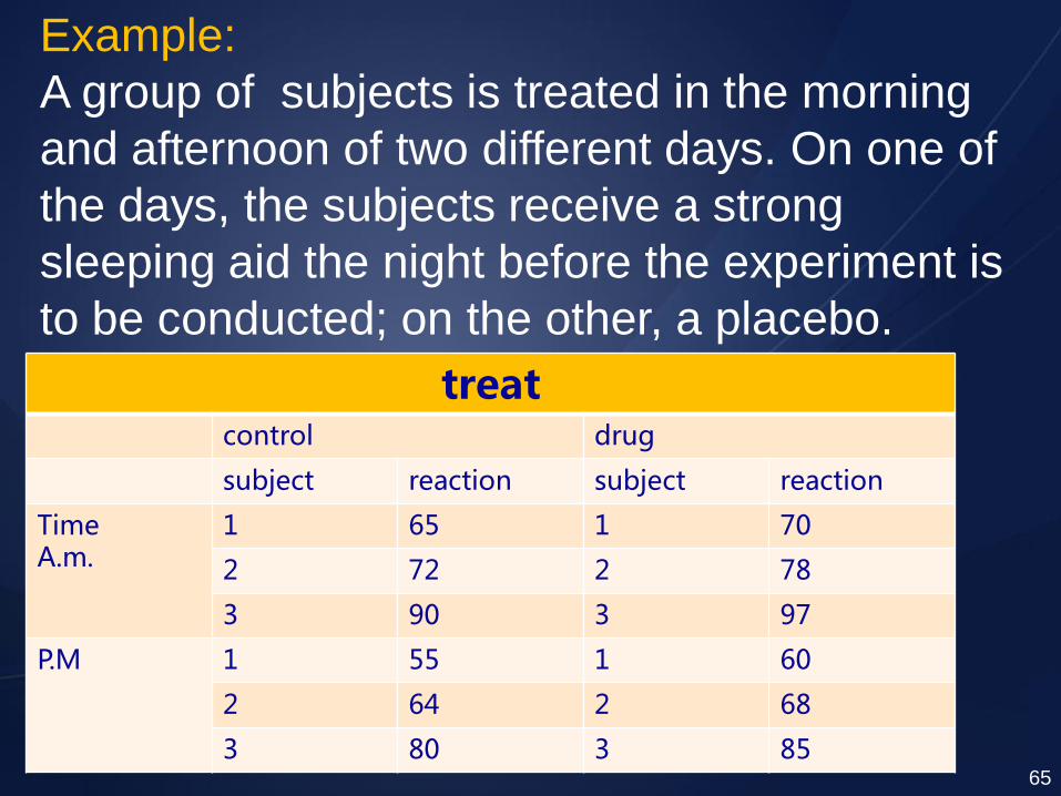
Example:
A group of subjects is treated in the morning
and afternoon of two different days. On one of
the days, the subjects receive a strong
sleeping aid the night before the experiment is
to be conducted; on the other, a placebo. treat
control drug
subject reaction subject reaction
Time A.m.
1 65 1 70
2 72 2 78
3 90 3 97
P.M 1 55 1 60
2 64 2 68
3 80 3 85 65
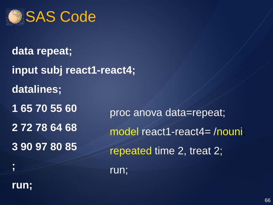
data repeat;
input subj react1-react4;
datalines;
1 65 70 55 60
2 72 78 64 68
3 90 97 80 85
;
run;
SAS Code
proc anova data=repeat;
model react1-react4= /nouni;
repeated time 2, treat 2;
run;
66
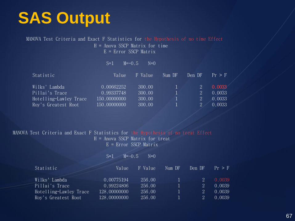
SAS Output
67
MANOVA Test Criteria and Exact F Statistics for the Hypothesis of no time Effect H = Anova SSCP Matrix for time E = Error SSCP Matrix S=1 M=-0.5 N=0 Statistic Value F Value Num DF Den DF Pr > F Wilks' Lambda 0.00662252 300.00 1 2 0.0033 Pillai's Trace 0.99337748 300.00 1 2 0.0033 Hotelling-Lawley Trace 150.00000000 300.00 1 2 0.0033 Roy's Greatest Root 150.00000000 300.00 1 2 0.0033
MANOVA Test Criteria and Exact F Statistics for the Hypothesis of no treat Effect H = Anova SSCP Matrix for treat E = Error SSCP Matrix S=1 M=-0.5 N=0 Statistic Value F Value Num DF Den DF Pr > F Wilks' Lambda 0.00775194 256.00 1 2 0.0039 Pillai's Trace 0.99224806 256.00 1 2 0.0039 Hotelling-Lawley Trace 128.00000000 256.00 1 2 0.0039 Roy's Greatest Root 128.00000000 256.00 1 2 0.0039
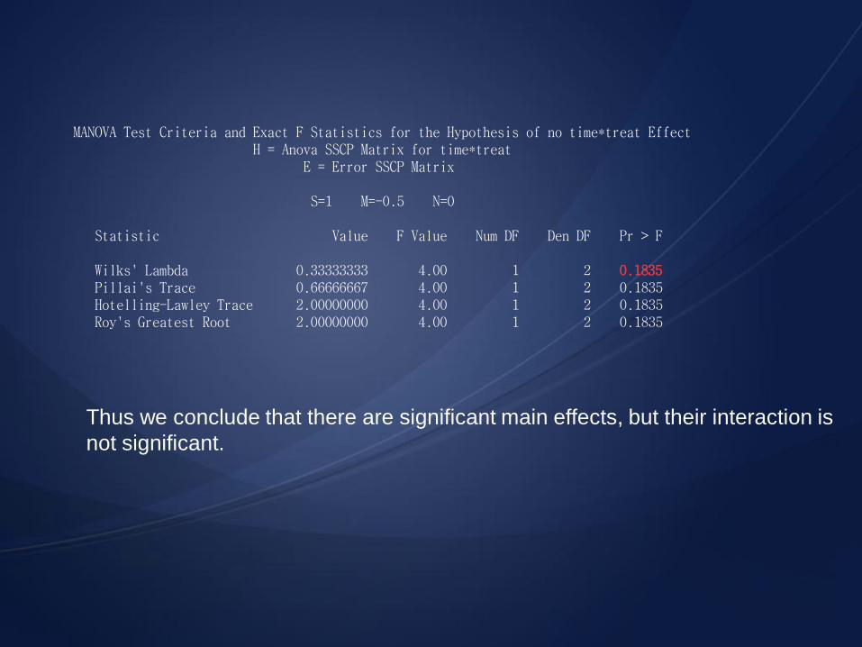
MANOVA Test Criteria and Exact F Statistics for the Hypothesis of no time*treat Effect H = Anova SSCP Matrix for time*treat E = Error SSCP Matrix S=1 M=-0.5 N=0 Statistic Value F Value Num DF Den DF Pr > F Wilks' Lambda 0.33333333 4.00 1 2 0.1835 Pillai's Trace 0.66666667 4.00 1 2 0.1835 Hotelling-Lawley Trace 2.00000000 4.00 1 2 0.1835 Roy's Greatest Root 2.00000000 4.00 1 2 0.1835
Thus we conclude that there are significant main effects, but their interaction is
not significant.

Interpretation According to the observed p-values, except
for the interactions, we can reject the
hypotheses that time and treat are not
significantly different.
The drug increase reaction time
Reaction time is longer in the morning
compared to the afternoon
The interaction of treat and time is not
significant
69
70
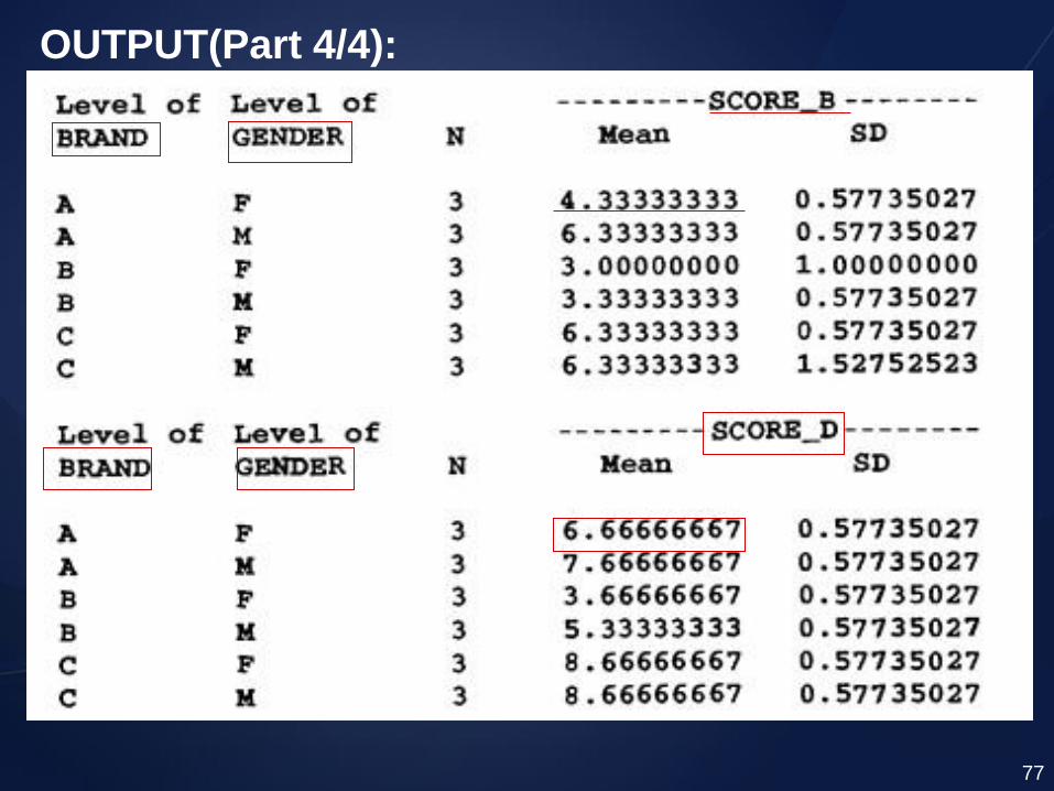
Consider a marketing experiment: Male and female subjects are offered one of three different brands of coffee.
Each brand is tasted twice; once after breakfast, the other time after dinner.
The preference of each brand is
measured on a scale from 1 to 10
(1=lowest, 10=highest). 71
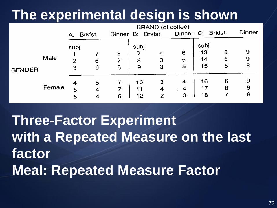
The experimental design is shown
below:
Three-Factor Experiment
with a Repeated Measure on the last
factor
Meal: Repeated Measure Factor
72
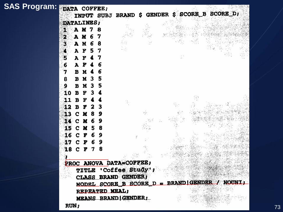
SAS Program:
73
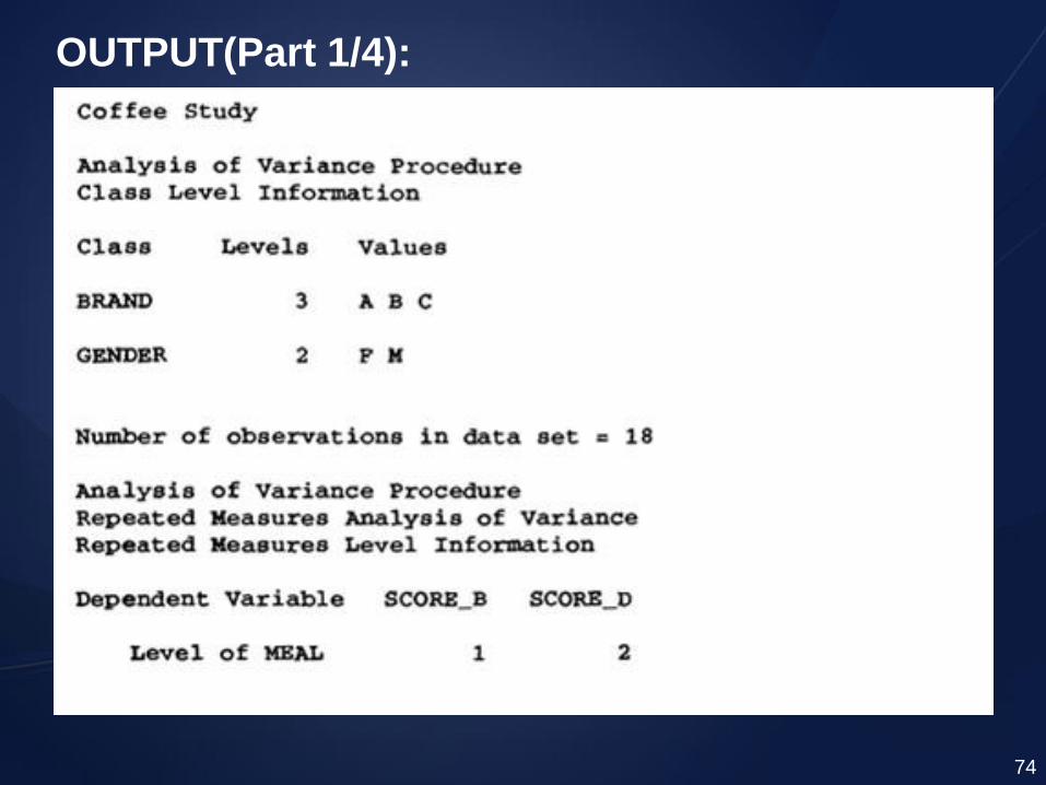
OUTPUT(Part 1/4):
74
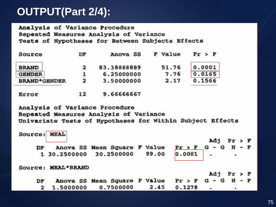
OUTPUT(Part 2/4):
75
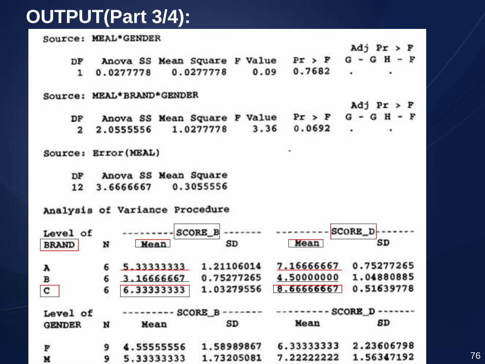
OUTPUT(Part 3/4):
76
OUTPUT(Part 4/4):
77
78
79
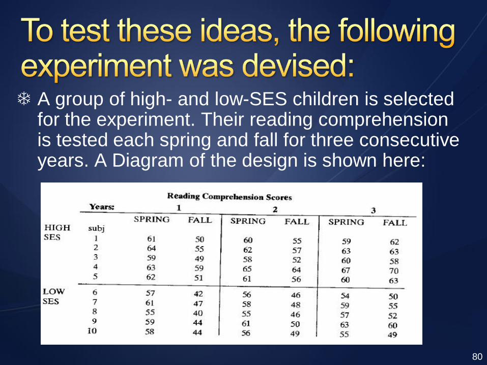
A group of high- and low-SES children is selected for the experiment. Their reading comprehension is tested each spring and fall for three consecutive years. A Diagram of the design is shown here:
80
81
Notice that each subject is measured every spring and fall of each year so that the variables SEASON and YEAR are both repeated measures factors.
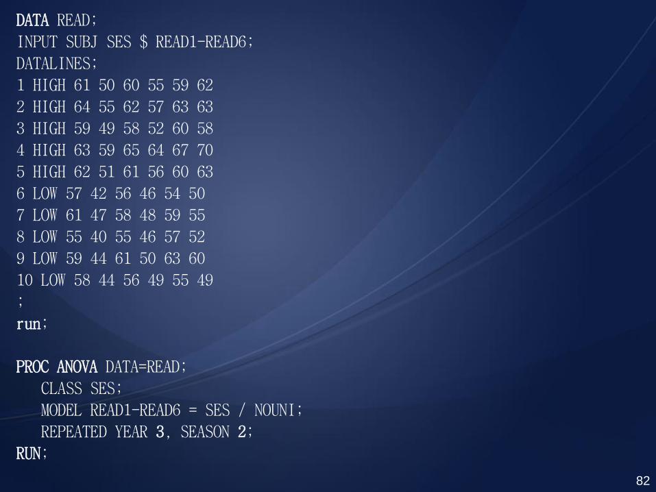
DATA READ;
INPUT SUBJ SES $ READ1-READ6;
DATALINES;
1 HIGH 61 50 60 55 59 62
2 HIGH 64 55 62 57 63 63
3 HIGH 59 49 58 52 60 58
4 HIGH 63 59 65 64 67 70
5 HIGH 62 51 61 56 60 63
6 LOW 57 42 56 46 54 50
7 LOW 61 47 58 48 59 55
8 LOW 55 40 55 46 57 52
9 LOW 59 44 61 50 63 60
10 LOW 58 44 56 49 55 49
;
run;
PROC ANOVA DATA=READ;
CLASS SES;
MODEL READ1-READ6 = SES / NOUNI;
REPEATED YEAR 3, SEASON 2;
RUN;
82
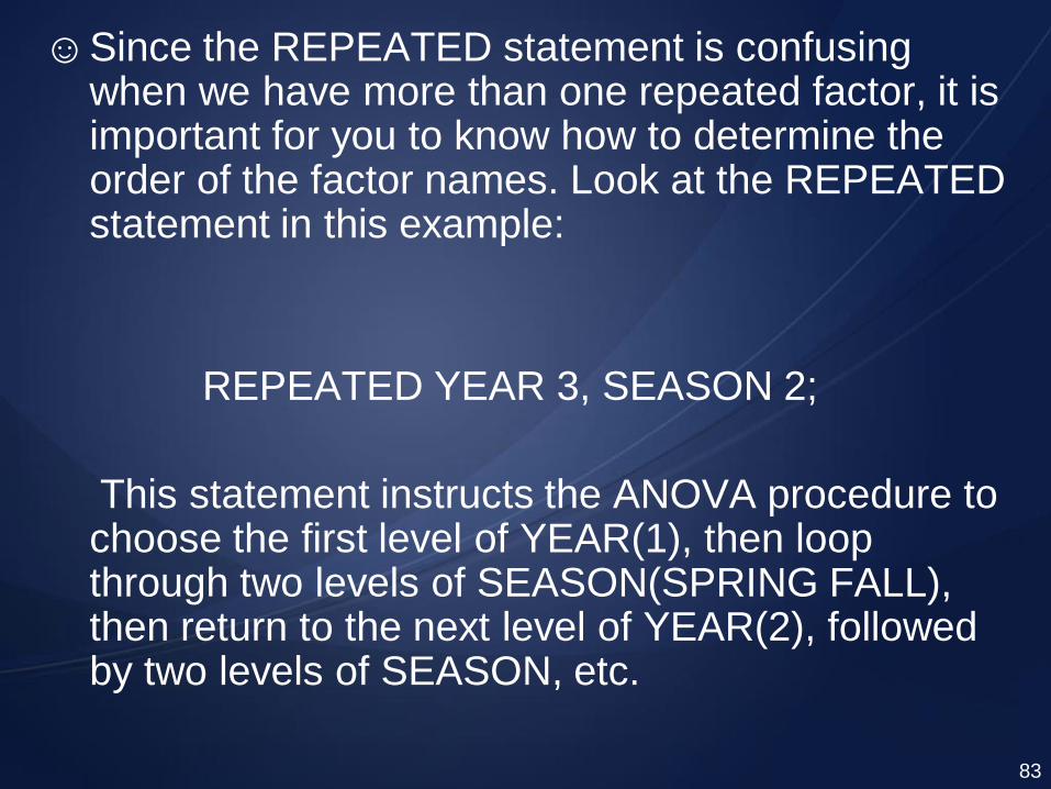
☺Since the REPEATED statement is confusing when we have more than one repeated factor, it is important for you to know how to determine the order of the factor names. Look at the REPEATED statement in this example:
REPEATED YEAR 3, SEASON 2;
This statement instructs the ANOVA procedure to choose the first level of YEAR(1), then loop through two levels of SEASON(SPRING FALL), then return to the next level of YEAR(2), followed by two levels of SEASON, etc.
83
84
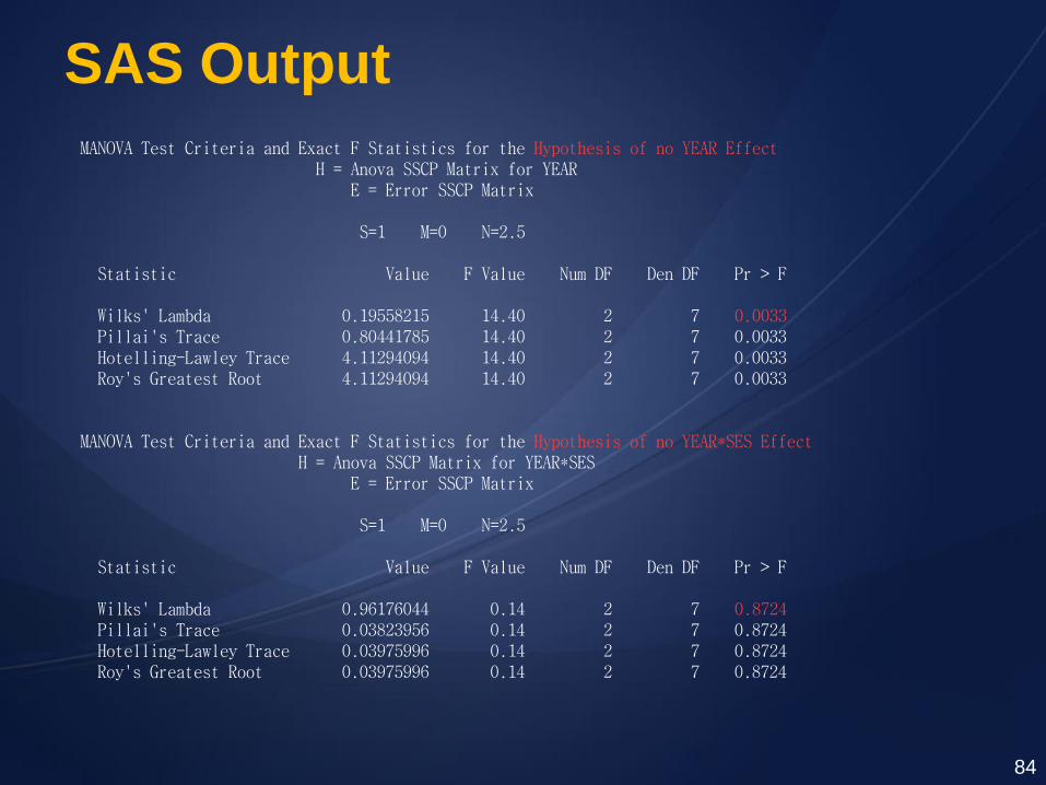
SAS Output
MANOVA Test Criteria and Exact F Statistics for the Hypothesis of no YEAR Effect H = Anova SSCP Matrix for YEAR E = Error SSCP Matrix S=1 M=0 N=2.5 Statistic Value F Value Num DF Den DF Pr > F Wilks' Lambda 0.19558215 14.40 2 7 0.0033 Pillai's Trace 0.80441785 14.40 2 7 0.0033 Hotelling-Lawley Trace 4.11294094 14.40 2 7 0.0033 Roy's Greatest Root 4.11294094 14.40 2 7 0.0033 MANOVA Test Criteria and Exact F Statistics for the Hypothesis of no YEAR*SES Effect H = Anova SSCP Matrix for YEAR*SES E = Error SSCP Matrix S=1 M=0 N=2.5 Statistic Value F Value Num DF Den DF Pr > F Wilks' Lambda 0.96176044 0.14 2 7 0.8724 Pillai's Trace 0.03823956 0.14 2 7 0.8724 Hotelling-Lawley Trace 0.03975996 0.14 2 7 0.8724 Roy's Greatest Root 0.03975996 0.14 2 7 0.8724
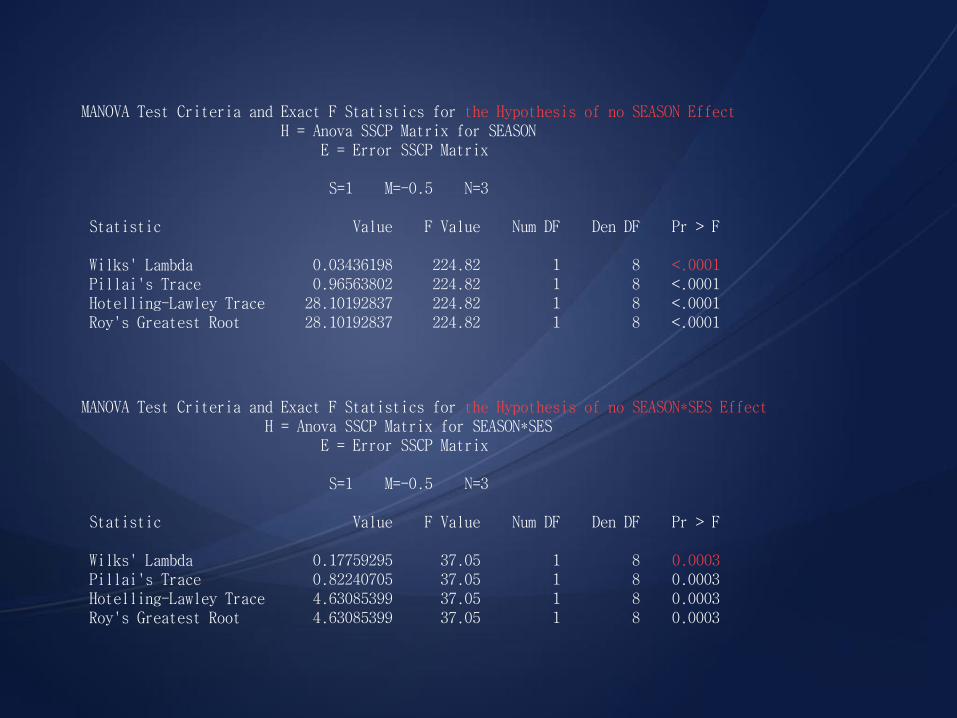
MANOVA Test Criteria and Exact F Statistics for the Hypothesis of no SEASON Effect H = Anova SSCP Matrix for SEASON E = Error SSCP Matrix S=1 M=-0.5 N=3 Statistic Value F Value Num DF Den DF Pr > F Wilks' Lambda 0.03436198 224.82 1 8 <.0001 Pillai's Trace 0.96563802 224.82 1 8 <.0001 Hotelling-Lawley Trace 28.10192837 224.82 1 8 <.0001 Roy's Greatest Root 28.10192837 224.82 1 8 <.0001
MANOVA Test Criteria and Exact F Statistics for the Hypothesis of no SEASON*SES Effect H = Anova SSCP Matrix for SEASON*SES E = Error SSCP Matrix S=1 M=-0.5 N=3 Statistic Value F Value Num DF Den DF Pr > F Wilks' Lambda 0.17759295 37.05 1 8 0.0003 Pillai's Trace 0.82240705 37.05 1 8 0.0003 Hotelling-Lawley Trace 4.63085399 37.05 1 8 0.0003 Roy's Greatest Root 4.63085399 37.05 1 8 0.0003
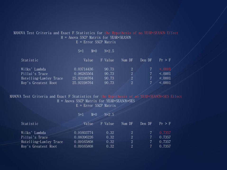
MANOVA Test Criteria and Exact F Statistics for the Hypothesis of no YEAR*SEASON Effect H = Anova SSCP Matrix for YEAR*SEASON E = Error SSCP Matrix S=1 M=0 N=2.5 Statistic Value F Value Num DF Den DF Pr > F Wilks' Lambda 0.03714436 90.73 2 7 <.0001 Pillai's Trace 0.96285564 90.73 2 7 <.0001 Hotelling-Lawley Trace 25.92198764 90.73 2 7 <.0001 Roy's Greatest Root 25.92198764 90.73 2 7 <.0001 MANOVA Test Criteria and Exact F Statistics for the Hypothesis of no YEAR*SEASON*SES Effect H = Anova SSCP Matrix for YEAR*SEASON*SES E = Error SSCP Matrix S=1 M=0 N=2.5 Statistic Value F Value Num DF Den DF Pr > F Wilks' Lambda 0.91603774 0.32 2 7 0.7357 Pillai's Trace 0.08396226 0.32 2 7 0.7357 Hotelling-Lawley Trace 0.09165808 0.32 2 7 0.7357 Roy's Greatest Root 0.09165808 0.32 2 7 0.7357
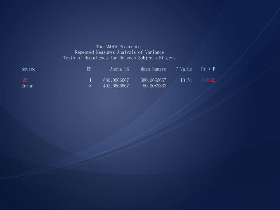
The ANOVA Procedure Repeated Measures Analysis of Variance Tests of Hypotheses for Between Subjects Effects Source DF Anova SS Mean Square F Value Pr > F SES 1 680.0666667 680.0666667 13.54 0.0062 Error 8 401.6666667 50.2083333
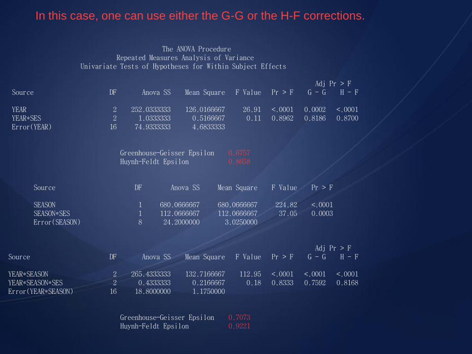
The ANOVA Procedure Repeated Measures Analysis of Variance Univariate Tests of Hypotheses for Within Subject Effects Adj Pr > F Source DF Anova SS Mean Square F Value Pr > F G - G H - F YEAR 2 252.0333333 126.0166667 26.91 <.0001 0.0002 <.0001 YEAR*SES 2 1.0333333 0.5166667 0.11 0.8962 0.8186 0.8700 Error(YEAR) 16 74.9333333 4.6833333 Greenhouse-Geisser Epsilon 0.6757 Huynh-Feldt Epsilon 0.8658 Source DF Anova SS Mean Square F Value Pr > F SEASON 1 680.0666667 680.0666667 224.82 <.0001 SEASON*SES 1 112.0666667 112.0666667 37.05 0.0003 Error(SEASON) 8 24.2000000 3.0250000 Adj Pr > F Source DF Anova SS Mean Square F Value Pr > F G - G H - F YEAR*SEASON 2 265.4333333 132.7166667 112.95 <.0001 <.0001 <.0001 YEAR*SEASON*SES 2 0.4333333 0.2166667 0.18 0.8333 0.7592 0.8168 Error(YEAR*SEASON) 16 18.8000000 1.1750000 Greenhouse-Geisser Epsilon 0.7073 Huynh-Feldt Epsilon 0.9221
In this case, one can use either the G-G or the H-F corrections.
We can use other SAS procedures
such as:
“Proc GLM”
“Proc Mixed”
Alternative SAS Procedures
for Repeated Measures ANOVA
89

My thanks go to:
My students!
Cody & Smith & their little SAS
book where several examples were
selected from.
Acknowledgement
90