Renormalization Group in perturbation theory and Callan...

Renormalization Group in perturbation theoryand Callan Symanzik eq.

Zhiguang Xiao

April 15, 2018

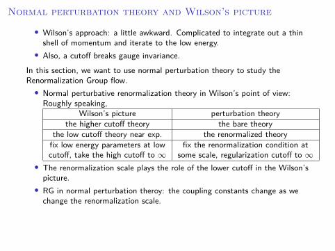
Normal perturbation theory and Wilson’s picture

• Wilson’s approach: a little awkward. Complicated to integrate out a thinshell of momentum and iterate to the low energy.

• Also, a cutoff breaks gauge invariance.In this section, we want to use normal perturbation theory to study theRenormalization Group flow.• Normal perturbative renormalization theory in Wilson’s point of view:

Roughly speaking,Wilson’s picture perturbation theory

the higher cutoff theory the bare theorythe low cutoff theory near exp. the renormalized theory

fix low energy parameters at low fix the renormalization condition atcutoff, take the high cutoff to ∞ some scale, regularization cutoff to ∞

• The renormalization scale plays the role of the lower cutoff in the Wilson’spicture.

• RG in normal perturbation theroy: the coupling constants change as wechange the renormalization scale.

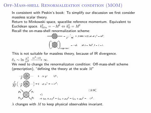
Off-Mass-shell Renormalization condition (MOM)In consistent with Peskin’s book: To simplify our discussion we first considermassless scalar theory.Return to Minkowski space, spacelike reference momentum. Equivalent toEuclidean space. k2

Min = −M2 ⇔ k2E = M2

Recall the on-mass-shell renormalization scheme:

This is not suitable for massless theory, because of IR divergence.δλ ∼ ln Λ2

m2m2→0−−−−→ ∞.

We need to change the renormalizaton condition: Off-mass-shell scheme(prescription), “defining the theory at the scale M”

λ changes with M to keep physical observables invariant.

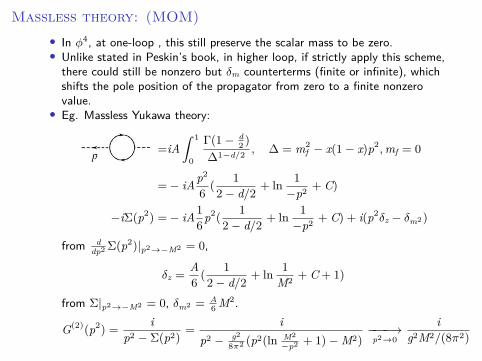
Massless theory: (MOM)• In ϕ4, at one-loop , this still preserve the scalar mass to be zero.• Unlike stated in Peskin’s book, in higher loop, if strictly apply this scheme,

there could still be nonzero but δm counterterms (finite or infinite), whichshifts the pole position of the propagator from zero to a finite nonzerovalue.

• Eg. Massless Yukawa theory:

=iA∫ 1

0

Γ(1 − d2 )

∆1−d/2 , ∆ = m2f − x(1 − x)p2,mf = 0

=− iAp2

6 (1

2 − d/2 + ln1

−p2 + C)

−iΣ(p2) =− iA16p2(

12 − d/2 + ln

1−p2 + C) + i(p2δz − δm2)

from ddp2 Σ(p2)|p2→−M2 = 0,

δz =A6 (

12 − d/2 + ln

1M2 + C + 1)

from Σ|p2→−M2 = 0, δm2 = A6 M2.

G(2)(p2) =i

p2 − Σ(p2)=

ip2 − g2

8π2 (p2(ln M2−p2 + 1)− M2)

−−−−→p2→0

ig2M2/(8π2)

• As is stated in Peskin’s book, “ the contribution to δm and δZ becometangled up with one another. Then it is awkward to define the masslesslimit.”

• If we still want p2 = 0 to be the physical pole, we can change the first twocondition:Σ(p2) = 0 at p2 = 0; 1

p2 Σ(p2) = 0 , at p2 = −M2.Then δm2 = 0 in the renormalized Lagrangian. Bare mass =0. This alsohappens in the massless ϕ4 theory.

• We impose the scalar mass to be zero by renormalization condition forsimiplicity. No dimensionful parameters in the Lagrangian.

• In dimensional regularizaton: no explicit quardratic divergence at d = 4:The integral:∫

ddk(2π)d

1p2 − m2 ∼ Γ(1 − d/2)

(m2)1−d/2m→0 first−−−−−−→

d→40

But at d = 2, it has a pole — the property of 4d quadratic divergence indimensional regularization. If we only consider d = 4, just set it to zero.The IR divergence and the UV divergence cancel.

• Another way:∫dDq

(−q2)α=i πD/2

Γ(D/2)

∫ ∞

0dQ2(Q2)D/2−α−1, (Wick rotation)

=i πD/2

Γ(D/2)

(∫ Λ

0dQ2(Q2)DIR/2−α−1 +

∫ ∞

Λ

dQ2(Q2)DUV/2−α−1)

=i πD/2

Γ(D/2)

(ΛDIR−2α

DIR2 − α

− ΛDUV−2α

DUV2 − α

), DIR > 2α,DUV < 2α

Analytically continue DIR and DUV to any dimension, then forDIR = DUV, the two terms cancel.

MOM

• In dimensional regularization, the 2/ϵ correspond to the log Λ2/M2 + Cdivergence in cutoff regulariztion. If we are only interested in the divergentpart, only replace 2/ϵ→ log Λ2/M2 + C, to emphasise the physical role ofthe cutoff.

• The second renormalization condition implies:

⟨Ω|ϕ(p)ϕ(−p)|Ω⟩ → ip2 =

i−M2 , at p2 → −M2

ϕ is not the physical field in the on-mass-shell renormalization scheme.The field in this offshell scheme is related with the bare fields byϕ = Z−1/2ϕ0. And we have

⟨Ω|ϕ0(p)ϕ0(−p)|Ω⟩ → iZp2 → iZ

−M2 at p2 = −M2.

Z is not the residue at the physical pole p2 = 0 of the bare two pointfunction.

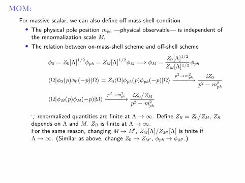
MOM:For massive scalar, we can also define off mass-shell condition• The physical pole position mph —physical observable— is independent of

the renormalization scale M.• The relation between on-mass-shell scheme and off-shell scheme

ϕ0 = Z0[Λ]1/2ϕph = ZM[Λ]1/2ϕM =⇒ ϕM =

Z0[Λ]1/2

ZM[Λ]1/2 ϕph

⟨Ω|ϕ0(p)ϕ0(−p)|Ω⟩ = Z0⟨Ω|ϕph(p)ϕph(−p)|Ω⟩p2→m2

ph−−−−−→ iZ0

p2 − m2ph

⟨Ω|ϕM(p)ϕM(−p)|Ω⟩p2→m2

ph−−−−−→ iZ0/ZM

p2 − m2ph

∵ renormalized quantities are finite at Λ → ∞. Define ZR = Z0/ZM, ZRdepends on Λ and M. ZR is finite at Λ → ∞.For the same reason, changing M → M′, ZM[Λ]/ZM′ [Λ] is finite ifΛ → ∞. (Similar as above, change Z0 → ZM′ , ϕph → ϕM′ .)

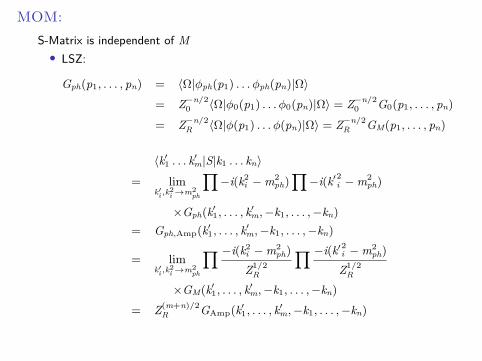
MOM:S-Matrix is independent of M• LSZ:

Gph(p1, . . . , pn) = ⟨Ω|ϕph(p1) . . . ϕph(pn)|Ω⟩= Z−n/2

0 ⟨Ω|ϕ0(p1) . . . ϕ0(pn)|Ω⟩ = Z−n/20 G0(p1, . . . , pn)

= Z−n/2R ⟨Ω|ϕ(p1) . . . ϕ(pn)|Ω⟩ = Z−n/2

R GM(p1, . . . , pn)

⟨k′1 . . . k′m|S|k1 . . . kn⟩

= limk′i ,k

2i →m2

ph

∏−i(k2

i − m2ph)∏

−i(k′2i − m2ph)

×Gph(k′1, . . . , k′m,−k1, . . . ,−kn)

= Gph,Amp(k′1, . . . , k′m,−k1, . . . ,−kn)

= limk′i ,k

2i →m2

ph

∏ −i(k2i − m2

ph)

Z1/2R

∏ −i(k′2i − m2ph)

Z1/2R

×GM(k′1, . . . , k′m,−k1, . . . ,−kn)

= Z(m+n)/2R GAmp(k′1, . . . , k′m,−k1, . . . ,−kn)

Changing renormalization scheme or renormalization scale

• In general, changing renormalization scheme or renormalization scale→ finite shifts of the renormalized parameters, λ, m2.

• The renormalization conditions:how the bare quantities → renormalized quantities + counterterms.

• Bare quantites: depends on cutoff Λ or ϵ, independent of therenormalization scale M.

• Changing the renormalization conditions: for eg. changing M or changingscheme, will change the relation between renormalized quantites and barequantites,As a result, Z relating bare and renormalized quantities, depends on Mand renormaliztion scheme.

• Renormalized Green’s functions also change with M — Callan-Symanzikequation.

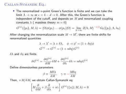
Callan-Symanzik Eq.:• The renormalized n-point Green’s function is finite and we can take the

limit Λ → ∞ or ϵ = 4 − d → 0. After this, the Green’s function isindependent of the cutoff, and depends on M and renormalized couplingconstants λ ( massless theory m = 0)G(n)(pi,M, λ) = ⟨Ω|ϕ(p1) . . . ϕ(pn)|Ω⟩ = lim

Λ→∞Z(Λ,M)−n/2G0(pi,Λ, λ0)

After changing the renormalization scale M → M′, there are finite shifts forrenormalized quantities

λ→ λ′ = λ+ δλ, ϕ→ ϕ′ = (1 + δη)ϕ

G(n) → G(n) = (1 + nδη)G(n)

δλ and δη are finite.

δG(n) =∂G(n)

∂M δM +∂G(n)

∂λδλ = nδηG(n)

Define dimensionless parameters

β ≡ Mδλ

δM , γ ≡ −Mδη

δMThen, ×M/δM, we obtain Callan-Symanzik eq:[

M ∂

∂M + β∂

∂λ+ nγ

]G(n)(xi;M, λ) = 0

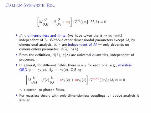
Callan-Symanzik Eq.:

[M ∂

∂M + β∂

∂λ+ nγ

]G(n)(xi;M, λ) = 0

• β, γ dimensionless and finite, (we have taken the Λ → ∞ limit)independent of Λ. Without other dimensionful parameters except M, bydimensional analysis, β, γ are independent of M — only depends ondimensionless parameter: β(λ), γ(λ).

• From the definition, β(λ), γ(λ) are universal quantities, independent ofprocesses.

• In general, for different fields, there is a γ for each one. e.g., masslessQED ψ — γ2(e), Aµ — γ3(e), C-S eq:[

M ∂

∂M + β(e) ∂∂λ

+ nγ2(e) + mγ3(e)]

G(n,m)(xi;M, e) = 0

n, electron; m photon fields.• For massless theory with only dimensionless couplings, all above analysis is

similar.

Callan-Symanzik Eq.:Calculation of β and γ

Calculation of β, γ:Use C-S eq on conveniently chosen Green’s function whichcan be calculated perturbatively.e.g. one-loop β, γ in ϕ4 theory: we use the C-S eq on 2-point and 4-pointGreen’s function.

G(4)(pi;M, λ) =

(1)O(λ) (2)O(λ2) (3)O(λ2)

G(2)(p2;M, λ) =

(1′)O(1) (2′)O(λ1) (3′)O(λ1) (4′)O(λ2)

[M ∂

∂M︸︷︷︸on(3)∼O(λ2)

+ β∂

∂λ︸︷︷︸on(1)∼O(λ2)

+ 4γ︸︷︷︸on(1)∼O(λ3)

]G(4)(pi;M, λ) = 0

[M ∂

∂M + β∂

∂λ+ 2γ

]G(2)(p2;M, λ) = 0


Counting order: β(λ), γ(λ) : in ϕ4 theory, changing M, λ = λ′ + O(λ′2),ϕ = ϕ′(1 + O(λ′2)). β ∼ O(λ2), γ ∼ O(λ2).• One-loop, G(2), the two O(λ) terms ((2’) and (3’)) cancel. O(λ)

counterterm has no M dependence. The leading correction withcounterterms (M dependence) appears in O(λ2). Also these terms in theexternal leges of G(4) cancel.

• Look at one-loop G(4): ∂∂M acts on the counterterm ∼ O(λ2). γ act on

the leading order O(λ): ∼ O(λ3). β ∂∂λ

acts on O(λ): ∼ O(λ2), only thefirst two terms contribute to the leading order O(λ2).[

M ∂

∂M + β∂

∂λ

]G(4)(pi;M, λ) = 0

• look at G(2): ∂∂M acts on leading nonvarnishing counterterm at 2-loop

∼ O(λ2). β ∂∂λ

act on leading nonvarnishing counterterm at 2-loop O(λ2)∼ O(λ3). Nonzero leading γ terms— act on the leading tree level O(1).So the leading nonzero order is O(λ2) at two-loop, only the first and thethird terms contribute. So to one-loop O(λ) order γ is zero:γ = 0 + O(λ2) [

M ∂

∂M + 2γ]

G(2)(p2;M, λ) = 0


Calculate the β(λ) at one-loop:

G(4) =[−iλ+ (−iλ)2[iV(s) + iV(t) + iV(u)]− iδλ

] 4∏i=1

ip2

i

Renormalization condition: G(4) = −iλ at s = t = u = −M2, to one-loopO(λ2)

δλ = −λ23V(−M2) =3λ2

2(4π)d/2

∫ 1

0dx Γ(2 − d/2)

(x(1 − x)M2)2−d/2

=32

λ2

(4π)2

[ 12 − d/2 − logM2

︸︷︷︸log Λ2

M2

+ finite terms︸︷︷︸independent of M

]

From C-S eq:[M ∂

∂M + β ∂∂λ

]G(4)(pi;M, λ) = 0

β∂

∂λ(−iλ) = −M ∂

∂M (−iδλ) ⇒ β(λ) =3λ2

(4π)2 + O(λ3)

β = the coefficient before log Λ/M, determined by infinite term, at leadingorder, in massless theory.


For general renormalizable massless theory, to Leading nonzero order :

G(2)(p2;M, g) = ( loop diagrams) + . . .

=i

p2 +i

p2 (A logΛ2

−p2 + finite) + ip2 (ip

2δZ)i

p2 + . . .

The loop diagrams come with an −ip2 cancel one i/p2. A, dimensionlessconstant. Renormalization condition ⇒ δZ = A log Λ2

M2 +finite .[M ∂

∂M + β∂

∂g + 2γ]

G(2)(p2;M, g) = 0

To lowest order, M dependence only comes from δZ, (higher order there couldbe δg). β (at least O(g2)) terms act on loop contributions ∼ at least one orderhigher than the first term. So[

M ∂

∂M + 2γ]

G(2)(p2;M, g) = 0 ⇒ γ =12M ∂

∂MδZ = −A

At one-loop, γ only needs the coefficient before log Λ, the infinite term in thecounterterm. We do not need to be precise in the calculation, and only thecoefficient before the log Λ is ok. (Massless theory).

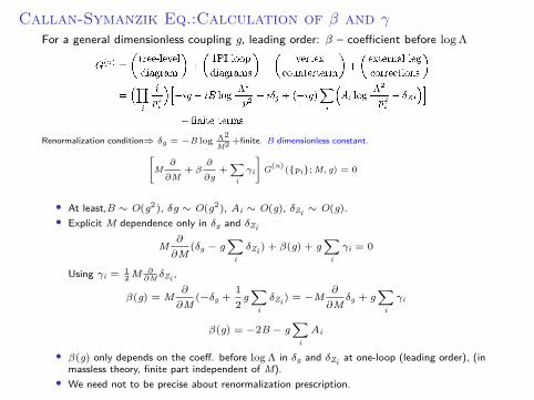
Callan-Symanzik Eq.:Calculation of β and γFor a general dimensionless coupling g, leading order: β – coefficient before log Λ

Renormalization condition⇒ δg = −B log Λ2M2 +finite. B dimensionless constant.[

M∂

∂M+ β

∂

∂g+

∑i

γi

]G(n)

(pi; M, g) = 0

• At least,B ∼ O(g2), δg ∼ O(g2), Ai ∼ O(g), δZi ∼ O(g).• Explicit M dependence only in δg and δZi

M∂

∂M(δg − g

∑i

δZi ) + β(g) + g∑

iγi = 0

Using γi =12 M ∂

∂M δZi ,

β(g) = M∂

∂M(−δg +

12

g∑

iδZi ) = −M

∂

∂Mδg + g

∑i

γi

β(g) = −2B − g∑

iAi

• β(g) only depends on the coeff. before log Λ in δg and δZi at one-loop (leading order), (inmassless theory, finite part independent of M).

• We need not to be precise about renormalization prescription.


Massless QED. ψ— γ2(e), Aµ—γ3(e).From chapt. 10.3,

L = −14 (F

µν)2 + iψ∂/ψ − eψA/ψ − 14δ3(Fµν)2 + iψδ2∂/ψ − eδ1ψA/ψ

δ2 = δ1 = −e2

(4π)d/2Γ(2 − d/2)(M2)2−d/2 + finite = −

e2

(4π)2

( 2ϵ

− ln M2+ finite

)

δ3 = −e2

(4π)d/243

Γ(2 − d/2)(M2)2−d/2 + finite = −

e2

(4π)d/243

( 2ϵ

− ln M2+ finite

)

C-S eq discussion, A little different: photon propagator(Feynman gauge):Dµν(q) = D(q)Pµν + −i

q2qµqν

q2 ; Pµν = gµν − qµqνq2 .

the last term depends on gauge, will drop out in gauge inv. observables. Weproject all external photon to transverse components D(q).

[M

∂

∂M+ β

∂

∂e+ 2γ3

]D(q2

; M, e) = 0 ⇒ γ3 =12

M∂

∂Mδ3 =

e2

12π2 ;

[M

∂

∂M+ β

∂

∂e+ 2γ2

]∆(q2

; M, e) = 0 ⇒ γ2 =12

M∂

∂Mδ2 =

e2

(4π)2 ;

[M

∂

∂M+ β

∂

∂e+ 2γ2 + γ3

]G(2,1)

µ = 0 ⇒ β(e) = M∂

∂M(−eδ1 + eδ2 +

12

eδ3) = eγ3 =e3

12π2

G(2,1)µ : Two fermion one photon Green’s function, projected to the transverse

part of the photon.

Callan-Symanzik Eq.:Meaning of β and γ

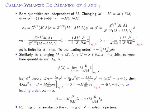
• Bare quantities are independent of M. Changing M → M′ = M + δM,ϕ→ ϕ′ = (1 + δη)ϕ, γ = −Mδη/δM:

ϕ0 = Z1/2(M,Λ)ϕ = Z′1/2(M + δM,Λ)ϕ′ ⇒ ϕ′ =

Z1/2(M,Λ)

Z′1/2(M + δM,Λ)ϕ

δη =Z1/2(M,Λ)

Z′1/2(M + δM,Λ)−1 = −1

2δMZ

∂

∂MZ∣∣∣∣λ0,Λ

⇒ γ = limΛ→∞

12

MZ

∂

∂MZ∣∣∣∣λ0,Λ

δη is finite for Λ → ∞. To the leading order, γ = 12 M ∂

∂MδZ• Simliarly, β: changing M → M′, λ→ λ′ = λ+ δλ, a finite shift, to keep

bare quantities inv. λ0, Λ.

β(λ) = limΛ→∞

M ∂

∂Mλ

∣∣∣∣λ0,Λ

Eg. ϕ4 theory: LB ∼ λ04! ϕ

40 = λ0

4! Z2ϕ4 = λ+δλ4! ϕ4 ⇒ λ0Z2 = λ+ δλ then

4λ0Z2γ = β + M ∂∂Mδλ

∣∣∣λ0,Λ

⇒ β = −M ∂∂Mδλ

∣∣∣λ0,Λ

+ 4(λ+ δλ)γ. toleading order, λ0 → λ,

β = −M ∂

∂Mδλ + 2λM ∂

∂MδZ

• Running of λ: similar to the running of λ′ in wilson’s picture.

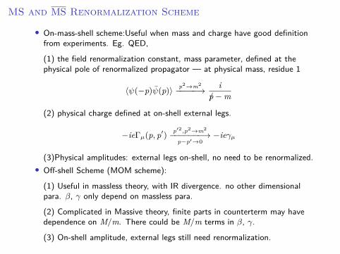
MS and MS Renormalization Scheme

• On-mass-shell scheme:Useful when mass and charge have good definitionfrom experiments. Eg. QED,

(1) the field renormalization constant, mass parameter, defined at thephysical pole of renormalized propagator — at physical mass, residue 1

⟨ψ(−p)ψ(p)⟩ p2→m2−−−−−→ i

p/− m

(2) physical charge defined at on-shell external legs.

−ieΓµ(p, p′)p′2,p2→m2−−−−−−−→

p−p′→0−ieγµ

(3)Physical amplitudes: external legs on-shell, no need to be renormalized.• Off-shell Scheme (MOM scheme):

(1) Useful in massless theory, with IR divergence. no other dimensionalpara. β, γ only depend on massless para.

(2) Complicated in Massive theory, finite parts in counterterm may havedependence on M/m. There could be M/m terms in β, γ.

(3) On-shell amplitude, external legs still need renormalization.

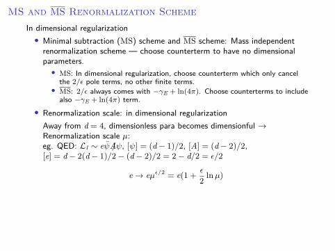
MS and MS Renormalization SchemeIn dimensional regularization• Minimal subtraction (MS) scheme and MS scheme: Mass independent

renormalization scheme — choose counterterm to have no dimensionalparameters.

• MS: In dimensional regularization, choose counterterm which only cancelthe 2/ϵ pole terms, no other finite terms.

• MS: 2/ϵ always comes with −γE + ln(4π). Choose counterterms to includealso −γE + ln(4π) term.

• Renormalization scale: in dimensional regularizationAway from d = 4, dimensionless para becomes dimensionful →Renormalization scale µ:eg. QED: LI ∼ eψA/ψ, [ψ] = (d − 1)/2, [A] = (d − 2)/2,[e] = d − 2(d − 1)/2 − (d − 2)/2 = 2 − d/2 = ϵ/2

e → eµϵ/2 = e(1 +ϵ

2 lnµ)

MS and MS Renormalization Schemee.g. QED.

−iΣ(p) =− i e2µϵΓ(2 − d/2)(4π)d/2 (−p/+ 4m) + finite + i(δ2p/− δm)

=− i e2

(4π)2

(2ϵ+ ln(4π)− γE + lnµ2

)(−p/+ 4m) + finite + i(δ2p/− δm)

MS δ2 = − e2

(4π)22ϵ, δm = − e2m

(4π)28ϵ

MS δ2 = − e2

(4π)2

(2ϵ− γE + ln(4π)

), δm = − e2m

(4π2)

(2ϵ− γE + ln(4π)

)Another formulation of MS: absorbing −γE + ln(4π) into µ2:e2 → e2(4π)−ϵ/2 expγEϵ/2µϵ = e2(1 + ϵ lnµ− ϵ

2 ln(4π) + ϵ2γE)

δ2 = − e2

(4π)22ϵ, δm = − e2m

(4π)28ϵ

Since there is no dimensionful parameter in the counterterms, it is convenientto discuss RG of massive theory using MS and MS scheme.

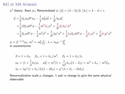
RG in MS Schemeϕ4 theory: Bare ϕ0; Renormalized ϕ; [ϕ] = (d − 2)/2; [λ0] = 4 − d = ϵ.

L =12∂µϕ0∂

µϕ0 − 12m2

0ϕ20 +

14!λ0ϕ

40

=12Z∂µϕ∂µϕ− 1

2m2Zmϕ2 +

14!Z4λµ

ϵϕ4

=12∂µϕ∂

µϕ− 12m2ϕ2 +

14!λµ

ϵϕ4 +12δZ∂µϕ∂

µϕ− 12δmϕ

2 +14!δλµ

ϵϕ4

ϕ = Z−1/2ϕ0, m2 = m20

ZZm

, λ = λ0µ−ϵ Z2

Z4in counterterms:

Z = 1 + δZ, Zm = 1 + δm/m2, Z4 = 1 + δλ/λ,

ϕ0 = (1 +12δZ)ϕ, m2

0 = m2(1 +1

m2 δm)(1 − δZ) = m2 + δm − m2δZ,

λ0 = λµϵ(1 + δλ/λ)(1 − 2δZ) = µϵ(λ+ δλ − 2λδZ)

Renormalization scale µ changes, λ and m change to give the same physicalobservable.

RG in MS Scheme

• In MS scheme, Z, Zm, Z4 depend on µ implicitly through λ, not explicitly.• Renormalized 1PI or connected n-point Green’s function:

Γ(n)(pi, λ,m, µ, ϵ) = Zn/2(λ, ϵ)Γ(n)0 (pi, λ0,m0, ϵ)

ϵ→0−−−→ finite

l.h.s :(1) renormalized, finite in ϵ→ 0 limit, expanded w.r.t ϵ, positive powers.(2) Explicitly depends on µ.r.h.s.:(1) Z depends on µ implicitly through λ, not explicitly.(2) Γ0: no dependence on µ.(3) Z has 1/ϵ pole which should cancel with poles in Γ0.

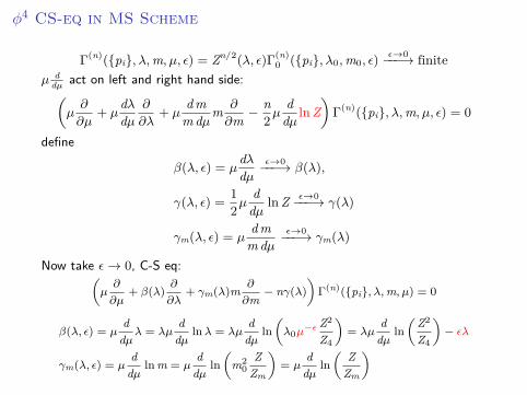
ϕ4 CS-eq in MS Scheme

Γ(n)(pi, λ,m, µ, ϵ) = Zn/2(λ, ϵ)Γ(n)0 (pi, λ0,m0, ϵ)

ϵ→0−−−→ finiteµ d

dµ act on left and right hand side:(µ∂

∂µ+ µ

dλdµ

∂

∂λ+ µ

d mm dµm ∂

∂m − n2µ

ddµ lnZ

)Γ(n)(pi, λ,m, µ, ϵ) = 0

define

β(λ, ϵ) = µdλdµ

ϵ→0−−−→ β(λ),

γ(λ, ϵ) =12µ

ddµ lnZ ϵ→0−−−→ γ(λ)

γm(λ, ϵ) = µd m

m dµϵ→0−−−→ γm(λ)

Now take ϵ→ 0, C-S eq:(µ∂

∂µ+ β(λ)

∂

∂λ+ γm(λ)m ∂

∂m− nγ(λ)

)Γ(n)(pi, λ,m, µ) = 0

β(λ, ϵ) = µd

dµλ = λµ

ddµ

lnλ = λµd

dµln

(λ0µ

−ϵ Z2

Z4

)= λµ

ddµ

ln

(Z2

Z4

)− ϵλ

γm(λ, ϵ) = µd

dµlnm = µ

ddµ

ln

(m2

0Z

Zm

)= µ

ddµ

ln

(Z

Zm

)

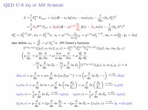
QED C-S eq in MS Scheme

L =14

Fµν0 F0,µν + ψ0(i∂/− e0A0/)ψ0 − m0ψ0ψ0 −

12ξ0

(∂µAµ0 )

2

=14

Z3FµνFµν + Z2ψ(i∂/− eµϵ/2 Z1Z2

A/)ψ − Zmmψψ −12ξ

(∂µAµ)2

Aµ0 = Z1/2

3 Aµ, ψ0 = Z1/22 ψ, e0 = µϵ/2e Z1

Z2Z1/23

= µϵ/2eZ−1/23 , m0 = m Zm

Z2, ξ0 = Z3ξ

also define α0 =e2

04π = µϵZ−1

3 α. 1PI Green’s function:Γ(n2,n3)(pi, α,m, ξ, µ, ϵ) = Zn2/2

2 Zn3/23 Γ

(n2,n3)0 (pi, α0,m0, ξ0, ϵ)(

µ∂

∂µ+ µ

dαdµ

∂

∂α+ µ

d mm dµ

m ∂

∂m+ µ

dξdµ

∂

∂ξ

−n22µ

ddµ

lnZ2 −n32µ

ddµ

lnZ3

)Γ(n2,n3)(pi, α,m, ξ, µ, ϵ) = 0

β(α, ϵ) = µd

dµα = µα

ddµ

ln(α0Z3µ

−ϵ)= α

(µ

ddµ

lnZ3 − ϵ

)ϵ→0−−−→ β(α)

γm(α, ϵ) = µd

dµlnm = µ

ddµ

ln

(m0

Z2Zm

)= µ

ddµ

ln

(Z2Zm

)ϵ→0−−−→ γm(α)

γ3(α, ϵ) =12µ

ddµ

lnZ3ϵ→0−−−→ γ3(α); γ2(α, ϵ) =

12µ

ddµ

lnZ2ϵ→0−−−→ γ2(α);

βξ(α, ϵ) = µd

dµξ = ξµ

ddµ

lnξ0Z3

= −ξµd

dµlnZ3 = ξγ3(α, ϵ)

ϵ→0−−−→ βξ = ξγ3(α)

QED C-S eq in MS Scheme

(µ∂

∂µ+ µ

dαdµ

∂

∂α+ µ

d mm dµm ∂

∂m + µdξdµ

∂

∂ξ

−n2

2 µd

dµ lnZ2 − n3

2 µd

dµ lnZ3

)Γ(n2,n3)(pi, α,m, ξ, µ, ϵ) = 0

take ϵ→ 0, C-S Eq.:(µ∂

∂µ+ β

∂

∂α+ βξ

∂

∂ξ+ γmm ∂

∂m − n2γ2 − n3γ3

)Γ(n2,m3)(pi, α,m, ξ, µ) = 0

In MS scheme, Z’s are independent of ξ. β, γ, independent of ξ.

Remarks:

• We can do the same thing on any kind of Green’s function (QED externallegs projected to transverse), only the relations between bare andrenormalized ones are different.

• Also on any observable, which have no bare correspondence, onlyindependent of µ.

µd

dµO =

(µ∂

∂µ+ β(λ)

∂

∂λ+ γm(λ)m ∂

∂m

)O = 0

• MS is similar to MS scheme.

Calculation of β and γ in MS schemeConsider a general coupling constant: λ = λ0µ

−ϵZ−1λ .

In ϕ4, λ = λ0µ−ϵ Z2

Z4⇒ Zλ = Z4/Z2;

in QED, λ = α, α0 =e2

04π = µϵZ−1

3 α, ⇒ Zλ =Z2

1Z3Z2

2

β(λ, ϵ) = µd

dµλ = λµ

ddµ

ln(λ0µ−ϵZ−1

λ ) = −λµd

dµlnZλ − ϵλ = −λβ(λ, ϵ)

1Zλ

ddλ

Zλ − ϵλ

In perturbation theory, MS scheme, (∵ limϵ→0 β(λ, ϵ) = β(λ))Zλ = [1 +

∑ν>0

aν(λ)ϵν

], ai =∑

j≥1 aijλj, β(λ, ϵ) = β(λ) +

∑ν≥1 βνϵ

ν

β(λ, ϵ)︸︷︷︸β(λ)+β1ϵ+...

(Zλ︸︷︷︸

1+ a1ϵ

+...

+λd

dλZλ︸︷︷︸λ

a′1ϵ

+...

)+ ϵλZλ︸︷︷︸

ϵλ(1+ a1ϵ

+... )

= 0

• counting the ϵ order O(ϵn>1) = 0:

β(λ, ϵ) =− ϵλZλ

/(Zλ + λ

ddλZλ

)= −ϵλ(1 +

a1

ϵ+ . . . )

/(1 +

a1 + λa′1

ϵ+ . . . )

=− ϵλ(1 +a1

ϵ+ . . . )(1 − a1 + λa′

1ϵ

+ . . . )

β(λ, ϵ) = −ϵλ+ β(λ),

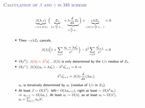
Calculation of β and γ in MS scheme

β(λ, ϵ)︸︷︷︸−ϵλ+β(λ)

(Zλ︸︷︷︸

1+ a1ϵ

+...

+λd

dλZλ︸︷︷︸λ

a′1ϵ

+...

)+ ϵλZλ︸︷︷︸

ϵλ(1+ a1ϵ

+... )

= 0

• Then −ϵλZλ cancels.

β(λ)(

1 +∑ν≥1

aν + λa′ν

ϵν

)− λ2∑

ν≥0

a′ν+1ϵν

= 0

• O(ϵ0): β(λ) = λ2a′1 , β(λ) is only determined by the 1/ϵ residue of Zλ.

• O(ϵν): β(λ)(aν + λa′ν)− λ2a′

ν+1 = 0 ⇒

λ2a′ν+1 = β(λ)

ddλ (λaν).

aν is iteratively determined by a1 (residue of 1/ϵ in Zλ).• At least β ∼ O(λ2). left∼ O(λaν+1), right at least ∼ O(λ2aν)

⇒ aν+1 ∼ O(λaν). At least a1 ∼ O(λ), so at least ai ∼ O(λi),ai =

∑j≥i aijλ

j.


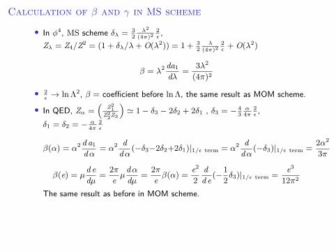
• In ϕ4, MS scheme δλ = 32

λ2

(4π)22ϵ,

Zλ = Z4/Z2 = (1 + δλ/λ+ O(λ2)) = 1 + 32

λ(4π)2

2ϵ+ O(λ2)

β = λ2 da1

dλ =3λ2

(4π)2

• 2ϵ→ lnΛ2, β = coefficient before lnΛ, the same result as MOM scheme.

• In QED, Zα =(

Z21

Z22Z3

)≃ 1 − δ3 − 2δ2 + 2δ1 , δ3 = − 4

3α

4π2ϵ,

δ1 = δ2 = − α4π

2ϵ

β(α) = α2 d a1

dα = α2 ddα (−δ3−2δ2+2δ1)|1/ϵ term = α2 d

dα (−δ3)|1/ϵ term =2α2

3π

β(e) = µd edµ =

2πe µ

dαdµ =

2πe β(α) =

e2

2dd e (−

12δ3)|1/ϵ term =

e3

12π2

The same result as before in MOM scheme.

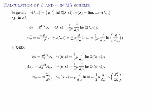
Calculation of β and γ in MS schemeIn general, γ(λ, ϵ) = 1

2µd

d µln(Z(λ, ϵ)). γ(λ) = limϵ→0 γ(λ, ϵ)

eg. in ϕ4,

ϕ0 = Z1/2ϕ, γ(λ, ϵ) =12µ

ddµ ln(Z(λ, ϵ));

m20 = m2 Zm

Z , γm(λ, ϵ) =12µ

ddµ lnm =

12µ

ddµ ln

(Z

Zm

);

in QED:

ψ0 = Z1/22 ψ, γ2(α, ϵ) =

12µ

ddµ ln(Z2(α, ϵ));

A0,µ = Z1/23 Aµ, γ3(α, ϵ) =

12µ

ddµ ln(Z3(α, ϵ));

m0 = mZm

Z2, γm(α, ϵ) = µ

ddµ lnm =

12µ

ddµ ln

(Z2

2Z2m

);

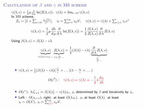
Calculation of β and γ in MS schemeγ(λ, ϵ) = 1

2µd

d µln(Z(λ, ϵ)). γ(λ) = limϵ→0 γ(λ, ϵ)

In MS scheme,Zλ = [1 +

∑ν>0

zν(λ)ϵν

], zi =∑∞

j=1 zijλj, γ(λ, ϵ) = γ(λ) +

∑ν≥1 γνϵ

ν

γ(λ, ϵ) =12µ

dλdµ

∂

∂ λln(Z(λ, ϵ)) = 1

2β(λ, ϵ)

Z(λ, ϵ)∂

∂ λZ(λ, ϵ)

Using β(λ, ϵ) = β(λ)− ϵλ

γ(λ, ϵ)︸︷︷︸γ(λ)+γ1ϵ...

Z(λ, ϵ)︸︷︷︸1+ z1

ϵ...

=12 (β(λ)− ϵλ)

∂

∂ λZ(λ, ϵ)︸︷︷︸z′1ϵ...

• γ(λ, ϵ) = 12 (β(λ)− ϵλ)(

z′1ϵ+ . . . )(1 − z1

ϵ+ . . . )

O(ϵ0) : γ(λ, ϵ) = γ(λ) = −12λ

dz1

dλ

• O(ϵν): λz′ν+1 = β(λ)z′ν − γ(λ)zν , zν determined by β and iteratively by z1.• Left : O(zν+1); right: at least O(λzν). z1 at least O(λ). at least

zi ∼ O(λi), zi =∑∞

j≥i zijλj.


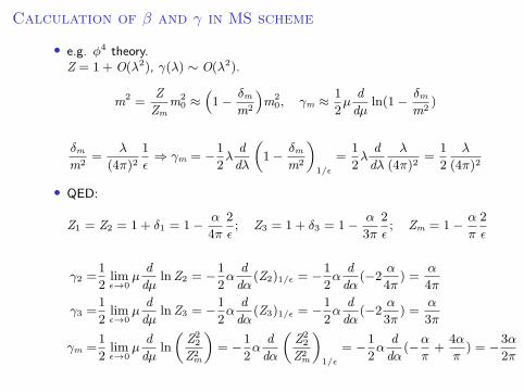
• e.g. ϕ4 theory.Z = 1 + O(λ2), γ(λ) ∼ O(λ2).

m2 =Z

Zmm2

0 ≈(

1 − δm

m2

)m2

0, γm ≈ 12µ

ddµ ln(1 − δm

m2 )

δm

m2 =λ

(4π)21ϵ⇒ γm = −1

2λd

dλ

(1 − δm

m2

)1/ϵ

=12λ

ddλ

λ

(4π)2 =12

λ

(4π)2

• QED:

Z1 = Z2 = 1 + δ1 = 1 − α

4π2ϵ; Z3 = 1 + δ3 = 1 − α

3π2ϵ; Zm = 1 − α

π

2ϵ

γ2 =12 lim

ϵ→0µ

ddµ lnZ2 = −1

2αd

dα (Z2)1/ϵ = −12α

ddα (−2 α4π ) =

α

4π

γ3 =12 lim

ϵ→0µ

ddµ lnZ3 = −1

2αd

dα (Z3)1/ϵ = −12α

ddα (−2 α3π ) =

α

3π

γm =12 lim

ϵ→0µ

ddµ ln

(Z2

2Z2m

)= −1

2αd

dα

(Z2

2Z2m

)1/ϵ

= −12α

ddα (−α

π+

4απ

) = −3α2π

Calculation of β and γ in MS schemeRemark:The mass independence of MS scheme has a shortcoming. It does not takeinto account of the decoupling of very massive particle.

If there is a very heavy particle in the theory and our exprimental energy scaleis less than the large mass, the massive particle is decoupled. At energy belowthe massive threshold we should not take into account of the contribution ofthis heavy particle in the loop.

More precise way is to use effective field method, integrate out the heavyparticle, and the heavy particle information is hidden in the coupling constant.(see e.g. Burgess hep-th/0701053)

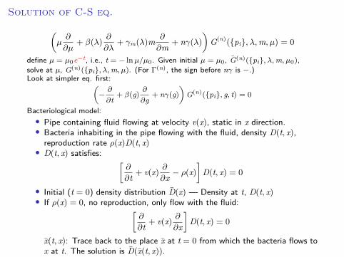
Solution of C-S eq.(µ∂

∂µ+ β(λ)

∂

∂λ+ γm(λ)m ∂

∂m + nγ(λ))

G(n)(pi, λ,m, µ) = 0

define µ = µ0e−t, i.e., t = − lnµ/µ0. Given initial µ = µ0, G(n)(pi, λ,m, µ0),solve at µ, G(n)(pi, λ,m, µ). (For Γ(n), the sign before nγ is −.)Look at simpler eq. first:(

−∂

∂t+ β(g) ∂

∂g+ nγ(g)

)G(n)(pi, g, t) = 0

Bacteriological model:• Pipe containing fluid flowing at velocity v(x), static in x direction.• Bacteria inhabiting in the pipe flowing with the fluid, density D(t, x),

reproduction rate ρ(x)D(t, x)• D(t, x) satisfies: [

∂

∂t + v(x) ∂∂x − ρ(x)

]D(t, x) = 0

• Initial (t = 0) density distribution D(x) — Density at t, D(t, x)• If ρ(x) = 0, no reproduction, only flow with the fluid:[

∂

∂t + v(x) ∂∂x

]D(t, x) = 0

x(t, x): Trace back to the place x at t = 0 from which the bacteria flows tox at t. The solution is D(x(t, x)).

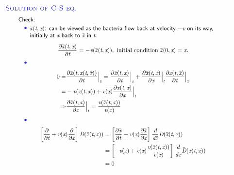
Solution of C-S eq.Check:• x(t, x): can be viewed as the bacteria flow back at velocity −v on its way,

initially at x back to x in t.

∂x(t, x)∂t = −v(x(t, x)), initial condition x(0, x) = x.

•

0 =∂x(t, x(t, x))

∂t

∣∣∣x=∂x(t, x)∂t

∣∣∣x+∂x(t, x)∂x

∣∣∣t

∂x(t, x)∂t

∣∣∣x

=− v(x(t, x)) + v(x)∂x(t, x)∂x

∣∣∣t

⇒∂x(t, x)∂x

∣∣∣t=

v(x(t, x))v(x)

• [∂

∂t + v(x) ∂∂x

]D(x(t, x)) =

[∂x∂t + v(x)∂x

∂x

]ddx D(x(t, x))

=

[−v(x) + v(x)v(x(t, x))

v(x)

]ddx D(x(t, x))

= 0

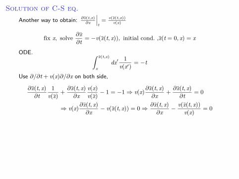
Solution of C-S eq.Another way to obtain: ∂x(t,x)

∂x

∣∣∣t= v(x(t,x))

v(x)

fix x, solve ∂x∂t = −v(x(t, x)), initial cond. ,x(t = 0, x) = x

ODE. ∫ x(t,x)

xdx′ 1

v(x′) = −t

Use ∂/∂t + v(x)∂/∂x on both side,

∂x(t, x)∂t

1v(x) +

∂x(t, x)∂x

v(x)v(x) − 1 = −1 ⇒ v(x)∂x(t, x)

∂x +∂x(t, x)∂t = 0

⇒ v(x)∂x(t, x)∂x − v(x(t, x)) = 0 ⇒ ∂x(t, x)

∂x − v(x(t, x))v(x) = 0

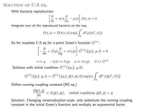
Solution of C-S eq.With bacteria reproduction:[

∂

∂t+ v(x) ∂

∂x− ρ(x)

]D(t, x) = 0

Integrate over all the reproduced bacteria on the way.

D(t, x) = D(x(t, x)) exp∫ t

0dt′ρ(x(t′, x))

So for massless C-S eq for n-point Green’s function G(n):[− ∂

∂t + β(g) ∂∂g + nγ(g)

]G(n)(pi, g, t) = 0

x ↔ g, −v(x) ↔ β(g), ρ↔ nγ(g), D ↔ G(n)

Solution with initial condition G(n)(pi, g, 0)

G(n)(pi, g, t) = G(n)(pi, g(t, g), 0) expn∫ t

0dt′γ(g(t′, β))

Define running coupling constant:(RG eq.)∂g(t, g)∂t = β(g(t, g)), initial condition g(0, g) = g

Solution: Changing renormalization scale, only substitute the running couplingconstant in the initial Green’s function and multiply an exponential factor.

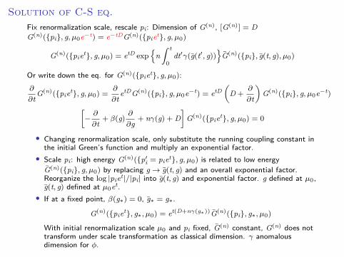
Solution of C-S eq.Fix renormalization scale, rescale pi: Dimension of G(n), [G(n)] = DG(n)(pi, g, µ0e−t) = e−tDG(n)(piet, g, µ0)

G(n)(piet, g, µ0) = etD exp

n∫ t

0dt′γ(g(t′, g))

G(n)(pi, g(t, g), µ0)

Or write down the eq. for G(n)(piet, g, µ0):∂

∂tG(n)(piet, g, µ0) =

∂

∂tetDG(n)(pi, g, µ0e−t) = etD

(D +

∂

∂t

)G(n)(pi, g, µ0e−t)

[−∂

∂t+ β(g) ∂

∂g+ nγ(g) + D

]G(n)(piet, g, µ0) = 0

• Changing renormalization scale, only substitute the running coupling constant inthe initial Green’s function and multiply an exponential factor.

• Scale pi: high energy G(n)(p′i = piet, g, µ0) is related to low energy

G(n)(pi, g, µ0) by replacing g → g(t, g) and an overall exponential factor.Reorganize the log |piet|/|pi| into g(t, g) and exponential factor. g defined at µ0,g(t, g) defined at µ0et.

• If at a fixed point, β(g∗) = 0, g∗ = g∗.

G(n)(piet, g∗, µ0) = et(D+nγ(g∗))G(n)(pi, g∗, µ0)

With initial renormalization scale µ0 and pi fixed, G(n) constant, G(n) does nottransform under scale transformation as classical dimension. γ anomalousdimension for ϕ.

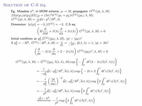
Solution of C-S eq.Eg. Massless ϕ4, in MOM scheme, µ→ M, propagator G(2)(|p|, λ,M).⟨Ω|ϕ(p1)ϕ(p2)|Ω⟩|M = (2π)4δ(4)(p1 + p2)G(2)(|p1|, λ,M);G(2)(|p|, λ,M) = i

p2 G(−p2/M2, λ)

Dimension: [ϕ(p)] = −3, [G(2)] = −2. C-S eq:(M ∂

∂M+ β(λ)

∂

∂λ+ 2γ(λ)

)G(2)(|p|, λ,M) = 0

Initial condition at p20,G(2)(|p0|, λ,M), |p| = |p0|et

if p20 = −M2, G(2)(−M2, λ,M) = i

p20= i

−M2 , G(1, λ) = 1; |p| = Met(∂

∂t− β(λ)

∂

∂λ+ 2 − 2γ(λ)

)G(2)(|p0|et, λ,M) = 0

G(2)(|p|, λ,M) = G(2)(|p0|, λ(t, λ),M) exp

−∫ t

0dt′(2 − 2γ(λ(t′, λ)))

=

i−p2

0G(−p2

0/M2, λ(t, λ)) exp− 2t + 2

∫ t

0dt′γ(λ(t′, λ))

= −

ip2

0

(|p||p0|

)−2G(−p2

0/M2, λ(t, λ)) exp

2∫ t


= −

ip2 G(−p2

0/M2, λ(t, λ)) exp

2∫ t


p2

0=−M2======== −

ip2 exp

2∫ t


Solution of C-S eq.

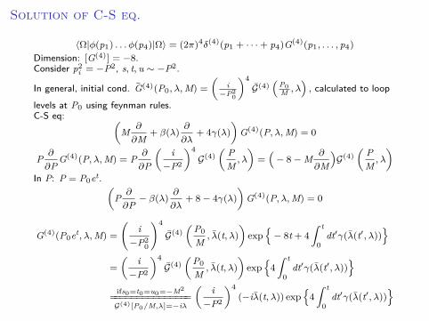
⟨Ω|ϕ(p1) . . . ϕ(p4)|Ω⟩ = (2π)4δ(4)(p1 + · · ·+ p4)G(4)(p1, . . . , p4)

Dimension: [G(4)] = −8.Consider p2

i = −P2, s, t, u ∼ −P2.

In general, initial cond. G(4)(P0, λ,M) =

(i

−P20

)4G(4)

(P0M , λ

), calculated to loop

levels at P0 using feynman rules.C-S eq: (

M ∂

∂M+ β(λ)

∂

∂λ+ 4γ(λ)

)G(4)(P, λ,M) = 0

P ∂

∂PG(4)(P, λ,M) = P ∂

∂P

(i

−P2

)4G(4)

(PM, λ

)=(− 8 − M ∂

∂M

)G(4)

(PM, λ

)In P: P = P0et. (

P ∂

∂P− β(λ)

∂

∂λ+ 8 − 4γ(λ)

)G(4)(P, λ,M) = 0

G(4)(P0et, λ,M) =

(i

−P20

)4

G(4)(

P0M, λ(t, λ)

)exp

− 8t + 4

∫ t


=

(i

−P2

)4G(4)

(P0M, λ(t, λ)

)exp

4∫ t


ifs0=t0=u0=−M2

===============G(4)[P0/M,λ]=−iλ

(i

−P2

)4(−iλ(t, λ)) exp

4∫ t


Solution of C-S eq.

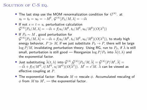
• The last step use the MOM renormalization condition for G(4). ats0 = t0 = u0 = −M2, G(4)[P0/M, λ] = −iλ

• If not s = t = u, perturbative calculationG(4)[P0/M, λ] = −iλ+ f(s0/M2, t0/M2, u0/M2)(O(λ2))

• If P0 ∼ M , good perturbation forG(4)[P0/M, λ] = −iλ+ f(s0/M2, t0/M2, u0/M2)(O(λ2)), to study highenergy behavior, P ≫ M, if we just substitute P0 → P, there will be largelogP/M, invalidating perturbation theory. Using RG, run to P0, if λ is stillsmall, perturbation is still good — Reorganize logP/P0 into λ(t, λ) andthe exponential factor.

• Just substituting λ(t, λ) into G(4),G(4)[P0/M, λ] = G(4)[P/M′, λ] =−iλ+ f(s/M′2, t/M′2, u/M′2)(O(λ2)). M′ = etM. λ can be viewed aseffective coupling at P.

• The exponential factor: Rescale M ⇒ rescale ϕ. Accumulated rescaling ofϕ from M to M′, — the exponential factor.

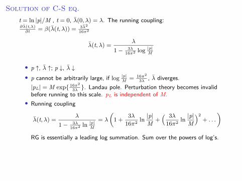
Solution of C-S eq.t = ln |p|/M , t = 0, λ(0, λ) = λ. The running coupling:∂λ(t,λ)

∂t = β(λ(t, λ)) = 3λ2

16π2

λ(t, λ) = λ

1 − 3λ16π2 log |p|

M

• p ↑, λ ↑; p ↓, λ ↓• p cannot be arbitrarily large, if log |p|

M = 16π2

3λ , λ diverges.|pL| = M exp 16π2

3λ . Landau pole. Perturbation theory becomes invalidbefore running to this scale. pL is independent of M.

• Running coupling

λ(t, λ) = λ

1 − 3λ16π2 ln |p|

M

= λ

(1 +

3λ16π2 ln

|p|M +

( 3λ16π2 ln

|p|M

)2+ . . .

)RG is essentially a leading log summation. Sum over the powers of log’s.

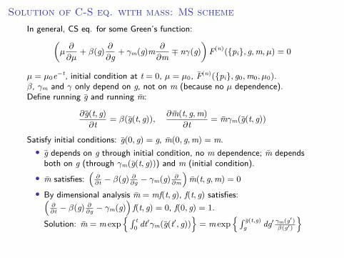
Solution of C-S eq. with mass: MS schemeIn general, CS eq. for some Green’s function:(

µ∂

∂µ+ β(g) ∂

∂g + γm(g)m ∂

∂m ∓ nγ(g))

F(n)(pi, g,m, µ) = 0

µ = µ0e−t, initial condition at t = 0, µ = µ0, F(n)(pi, g0,m0, µ0).β, γm and γ only depend on g, not on m (because no µ dependence).Define running g and running m:

∂g(t, g)∂t = β(g(t, g)), ∂m(t, g,m)

∂t = mγm(g(t, g))

Satisfy initial conditions: g(0, g) = g, m(0, g,m) = m.• g depends on g through initial condition, no m dependence; m depends

both on g (through γm(g(t, g))) and m (initial condition).• m satisfies:

(∂∂t − β(g) ∂

∂g − γm(g) ∂∂m

)m(t, g,m) = 0

• By dimensional analysis m = mf(t, g), f(t, g) satisfies:(∂∂t − β(g) ∂

∂g − γm(g))

f(t, g) = 0, f(0, g) = 1.

Solution: m = m exp∫ t

0 dt′γm(g(t′, g))= m exp

∫ g(t,g)g dg′ γm(g′)

β(g′)

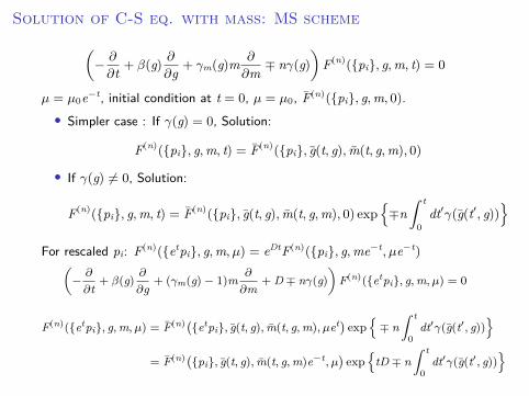
Solution of C-S eq. with mass: MS scheme(− ∂

∂t + β(g) ∂∂g + γm(g)m ∂

∂m ∓ nγ(g))

F(n)(pi, g,m, t) = 0

µ = µ0e−t, initial condition at t = 0, µ = µ0, F(n)(pi, g,m, 0).• Simpler case : If γ(g) = 0, Solution:

F(n)(pi, g,m, t) = F(n)(pi, g(t, g), m(t, g,m), 0)

• If γ(g) = 0, Solution:

F(n)(pi, g,m, t) = F(n)(pi, g(t, g), m(t, g,m), 0) exp∓n∫ t


For rescaled pi: F(n)(etpi, g,m, µ) = eDtF(n)(pi, g,me−t, µe−t)(

−∂

∂t+ β(g) ∂

∂g+ (γm(g)− 1)m ∂

∂m+ D ∓ nγ(g)

)F(n)(etpi, g,m, µ) = 0

F(n)(etpi, g,m, µ) = F(n)(etpi, g(t, g), m(t, g,m), µet) exp∓ n∫ t


= F(n)(pi, g(t, g), m(t, g,m)e−t, µ

)exp

tD ∓ n

∫ t


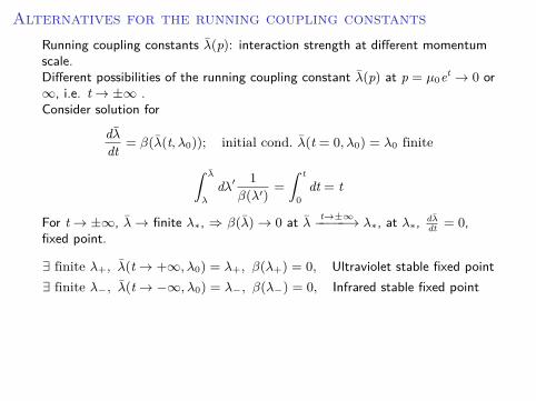
Alternatives for the running coupling constantsRunning coupling constants λ(p): interaction strength at different momentumscale.Different possibilities of the running coupling constant λ(p) at p = µ0et → 0 or∞, i.e. t → ±∞ .Consider solution for

dλdt = β(λ(t, λ0)); initial cond. λ(t = 0, λ0) = λ0 finite

∫ λ

λ

dλ′ 1β(λ′)

=

∫ t

0dt = t

For t → ±∞, λ→ finite λ∗, ⇒ β(λ) → 0 at λ t→±∞−−−−−→ λ∗, at λ∗, dλdt = 0,

fixed point.

∃ finite λ+, λ(t → +∞, λ0) = λ+, β(λ+) = 0, Ultraviolet stable fixed point∃ finite λ−, λ(t → −∞, λ0) = λ−, β(λ−) = 0, Infrared stable fixed point

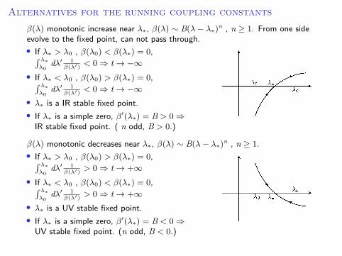
Alternatives for the running coupling constantsβ(λ) monotonic increase near λ∗, β(λ) ∼ B(λ− λ∗)

n , n ≥ 1. From one sideevolve to the fixed point, can not pass through.• If λ∗ > λ0 , β(λ0) < β(λ∗) = 0,∫ λ∗

λ0dλ′ 1

β(λ′) < 0 ⇒ t → −∞• If λ∗ < λ0 , β(λ0) > β(λ∗) = 0,∫ λ∗

λ0dλ′ 1

β(λ′) < 0 ⇒ t → −∞• λ∗ is a IR stable fixed point.• If λ∗ is a simple zero, β′(λ∗) = B > 0 ⇒

IR stable fixed point. ( n odd, B > 0.)

β(λ) monotonic decreases near λ∗, β(λ) ∼ B(λ− λ∗)n , n ≥ 1.

• If λ∗ > λ0 , β(λ0) > β(λ∗) = 0,∫ λ∗λ0

dλ′ 1β(λ′) > 0 ⇒ t → +∞

• If λ∗ < λ0 , β(λ0) < β(λ∗) = 0,∫ λ∗λ0

dλ′ 1β(λ′) > 0 ⇒ t → +∞

• λ∗ is a UV stable fixed point.• If λ∗ is a simple zero, β′(λ∗) = B < 0 ⇒

UV stable fixed point. (n odd, B < 0.)

Alternatives for the running coupling constantsFor a single coupling theory, λ∗ = 0 is always a fixed point.

• If λ = 0 is an IR stable fixed point — IR free theory.β(λ) > 0 at λ > 0 near zero. Perturbation valid nearλ = 0 at low energy scale.

• Possibility for λ away from λ∗ = 0, |p| ↑: λ larger,perturbation invalid,(1) New UV-fixed point developed. At this UV-fixedpoint, rescale momemtum p = p0et:G(n)(piet, λ∗, µ0) = et(D+nγ(λ∗))G(n)(pi, λ∗, µ0)

γ(λ∗) anomalous dimension.

eg : G(2)(p) ∼(

1p2

)1−γ(λ∗)

(2) No new fixed point.(a) λ→ ∞ as |p| → ∞.(b) λ→ ∞ at finite |p|.

∫∞λ0

dλ 1β(λ)

= tc finite.There should be a cut-off Λ, where new physics enters.

ϕ4, β(λ) = 3λ2

(4π)2 , IR-free, λ(p) = λ

1− 3λ16π2 log p

M, L.P. p = M exp 16π2

3λ .

QED β(e) = e3

12π2 , IR-free e2(p) = e2

1− e26π2 log(p/M)

, L.P. p = M exp 6πe2

Alternatives for the running coupling constants

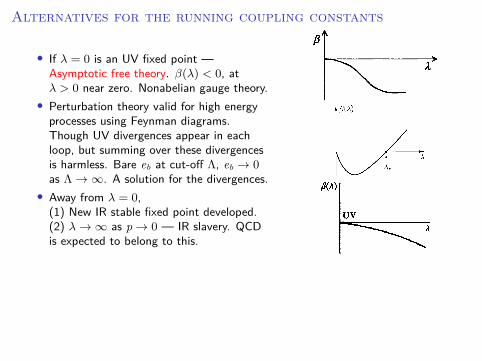
• If λ = 0 is an UV fixed point —Asymptotic free theory. β(λ) < 0, atλ > 0 near zero. Nonabelian gauge theory.

• Perturbation theory valid for high energyprocesses using Feynman diagrams.Though UV divergences appear in eachloop, but summing over these divergencesis harmless. Bare eb at cut-off Λ, eb → 0as Λ → ∞. A solution for the divergences.

• Away from λ = 0,(1) New IR stable fixed point developed.(2) λ→ ∞ as p → 0 — IR slavery. QCDis expected to belong to this.

Alternatives for the running coupling constantsLast case: β(λ) = 0 for any λ.• λ does not run with momentum scale. Bare λ is the renormalized one and

finite.• Field could still have infinite renormalization constant. Anomalous

dimension could still be nonzero.• S-matrix is automatically finite. — finite Quantum field theory.— N = 4

susy theory.

Renormalization Group in perturbation theory and Callan...

Documents

Transcript of Renormalization Group in perturbation theory and Callan...