Refining the clustering coefficient for analysis of …¬ning the clustering coefficient for...
8
ORIGINAL ARTICLE Refining the clustering coefficient for analysis of social and neural network data Roger Vargas 1 • Frank Garcea 2,3 • Bradford Z. Mahon 2,3,4 • Darren A. Narayan 5,6 Received: 16 February 2016 / Revised: 27 June 2016 / Accepted: 1 July 2016 Ó Springer-Verlag Wien 2016 Abstract In this paper we show how a deeper analysis of the clustering coefficient in a network can be used to assess functional connections in the human brain. Our metric of edge clustering centrality considers the frequency at which an edge appears across all local subgraphs that are induced by each vertex and its neighbors. This analysis is tied to a problem from structural graph theory in which we seek the largest subgraph that is a Cartesian product of two complete bipartite graphs K 1;m and K 1;1 . We investigate this property and compare it to other known edge centrality metrics. Finally, we apply the property of clustering centrality to an analysis of functional MRI data obtained, while healthy participants pantomimed object use or identified objects. Keywords Edge clustering centrality Functional MRI data Tool viewing Tool pantomiming Mathematics Subject Classification 05C12 90B18 1 Introduction In a social network, certain individuals are well connected and are more central to the network than others. Various centrality metrics have been investigated including betweenness centrality, closeness centrality, degree cen- trality, and eigenvalue centrality (Borgatti et al. 2013; Pavlopoulos et al. 2011). All of these metrics are linked to the same goal—finding a vertex (or vertices) that are most central within a network. However, one can also seek the edge (or edges) with the greatest centrality. This idea has been the topic of studies involving edge betweenness cen- trality (Girvan and Newman 2002; Newman 2010). The edge betweenness centrality of an edge e is the number of shortest paths between two vertices u and v that contain e, divided by the number of shortest paths between two ver- tices u and v, summed over all pairs of distinct vertices u and v. Another metric for assessing edge centrality is spanning edge centrality where the centrality of an edge is measured by the ratio of spanning trees that contain it. In this paper we introduce a new property, edge clustering centrality, which measures the centrality of edges in a network. A property that has been ubiquitous in social network literature has been the clustering coefficient (Holland and Leinhardt 1971; Watts and Strogatz 1998). For this property we consider the number of existing friendships in each per- son’s network (including themselves) compared to the total number of possible friendships within this local network. Then these quantities are averaged over all friends. This value is known as the clustering coefficient. In a sense, the clustering coefficient measures how closely knit a commu- nity network is. A deeper analysis of the clustering coeffi- cient can be conducted so that we can see which pair is most central to the network, that is, how many people know both people in a particular relationship? This has appeared in the & Darren A. Narayan [email protected] 1 Mathematics and Statistics, Williams College, Williamstown, USA 2 Department of Brain and Cognitive Sciences, University of Rochester, Rochester, USA 3 Center for Visual Science, University of Rochester, Rochester, USA 4 Department of Neurosurgery, University of Rochester, Medical Center, Rochester, USA 5 School of Mathematical Sciences, Rochester Institute of Technology, Rochester, NY, USA 6 Rochester Center for Brain Imaging, University of Rochester, Rochester, USA 123 Soc. Netw. Anal. Min. (2016)6:49 DOI 10.1007/s13278-016-0361-x
Transcript of Refining the clustering coefficient for analysis of …¬ning the clustering coefficient for...
ORIGINAL ARTICLE
Refining the clustering coefficient for analysis of social and neuralnetwork data
Roger Vargas1 • Frank Garcea2,3 • Bradford Z. Mahon2,3,4 • Darren A. Narayan5,6
Received: 16 February 2016 / Revised: 27 June 2016 / Accepted: 1 July 2016
� Springer-Verlag Wien 2016
Abstract In this paper we show how a deeper analysis of the
clustering coefficient in a network can be used to assess
functional connections in the human brain. Our metric of
edge clustering centrality considers the frequency at which
an edge appears across all local subgraphs that are induced by
each vertex and its neighbors. This analysis is tied to a
problem from structural graph theory in which we seek the
largest subgraph that is a Cartesian product of two complete
bipartite graphs K1;m and K1;1. We investigate this property
and compare it to other known edge centrality metrics.
Finally, we apply the property of clustering centrality to an
analysis of functional MRI data obtained, while healthy
participants pantomimed object use or identified objects.
Keywords Edge clustering centrality � Functional MRI
data � Tool viewing � Tool pantomiming
Mathematics Subject Classification 05C12 � 90B18
1 Introduction
In a social network, certain individuals are well connected
and are more central to the network than others. Various
centrality metrics have been investigated including
betweenness centrality, closeness centrality, degree cen-
trality, and eigenvalue centrality (Borgatti et al. 2013;
Pavlopoulos et al. 2011). All of these metrics are linked to
the same goal—finding a vertex (or vertices) that are most
central within a network. However, one can also seek the
edge (or edges) with the greatest centrality. This idea has
been the topic of studies involving edge betweenness cen-
trality (Girvan and Newman 2002; Newman 2010). The
edge betweenness centrality of an edge e is the number of
shortest paths between two vertices u and v that contain e,
divided by the number of shortest paths between two ver-
tices u and v, summed over all pairs of distinct vertices u and
v. Another metric for assessing edge centrality is spanning
edge centrality where the centrality of an edge is measured
by the ratio of spanning trees that contain it. In this paper we
introduce a new property, edge clustering centrality, which
measures the centrality of edges in a network.
A property that has been ubiquitous in social network
literature has been the clustering coefficient (Holland and
Leinhardt 1971; Watts and Strogatz 1998). For this property
we consider the number of existing friendships in each per-
son’s network (including themselves) compared to the total
number of possible friendships within this local network.
Then these quantities are averaged over all friends. This
value is known as the clustering coefficient. In a sense, the
clustering coefficient measures how closely knit a commu-
nity network is. A deeper analysis of the clustering coeffi-
cient can be conducted so that we can see which pair is most
central to the network, that is, how many people know both
people in a particular relationship? This has appeared in the
& Darren A. Narayan
1 Mathematics and Statistics, Williams College, Williamstown,
USA
2 Department of Brain and Cognitive Sciences, University of
Rochester, Rochester, USA
3 Center for Visual Science, University of Rochester,
Rochester, USA
4 Department of Neurosurgery, University of Rochester,
Medical Center, Rochester, USA
5 School of Mathematical Sciences, Rochester Institute of
Technology, Rochester, NY, USA
6 Rochester Center for Brain Imaging, University of Rochester,
Rochester, USA
123
Soc. Netw. Anal. Min. (2016) 6:49
DOI 10.1007/s13278-016-0361-x
social media, as noted in a New York Times article by Alex
Williams (www.nytimes.com/2014/08/14/fashion/power-
couples-on-twitter-and-instagram.html?_r=0), where celeb-
rity couples have been ‘‘leveraging their influence on social
media to frame themselves as a public unit, a powerfully
synchronous commodity.’’ As part of our analysis, we will
investigate the prominence of the influence of a pair in a
social network.
A classic example is at a wedding, where guests know
either the bride or the groom, and a large number of people
know both. In all likelihood, the wedding couple has the
most central relationship in the network (see Fig. 1).
We will call this type of analysis ‘‘clustering centrality’’
which is closely related to the clustering coefficient.
We begin by reviewing the property of the clustering
coefficient. The clustering coefficient (closed version) is
defined to be
CCðGÞ ¼ 1
n
Xi
2 EðGiÞj jVðGiÞj j � VðGiÞj j � 1ð Þ
where each local subgraph Gi is the subgraph which
includes the vertex i and all of its neighbors. The vertex
and edge sets of Gi will be denoted VðGiÞ and EðGiÞrespectively.
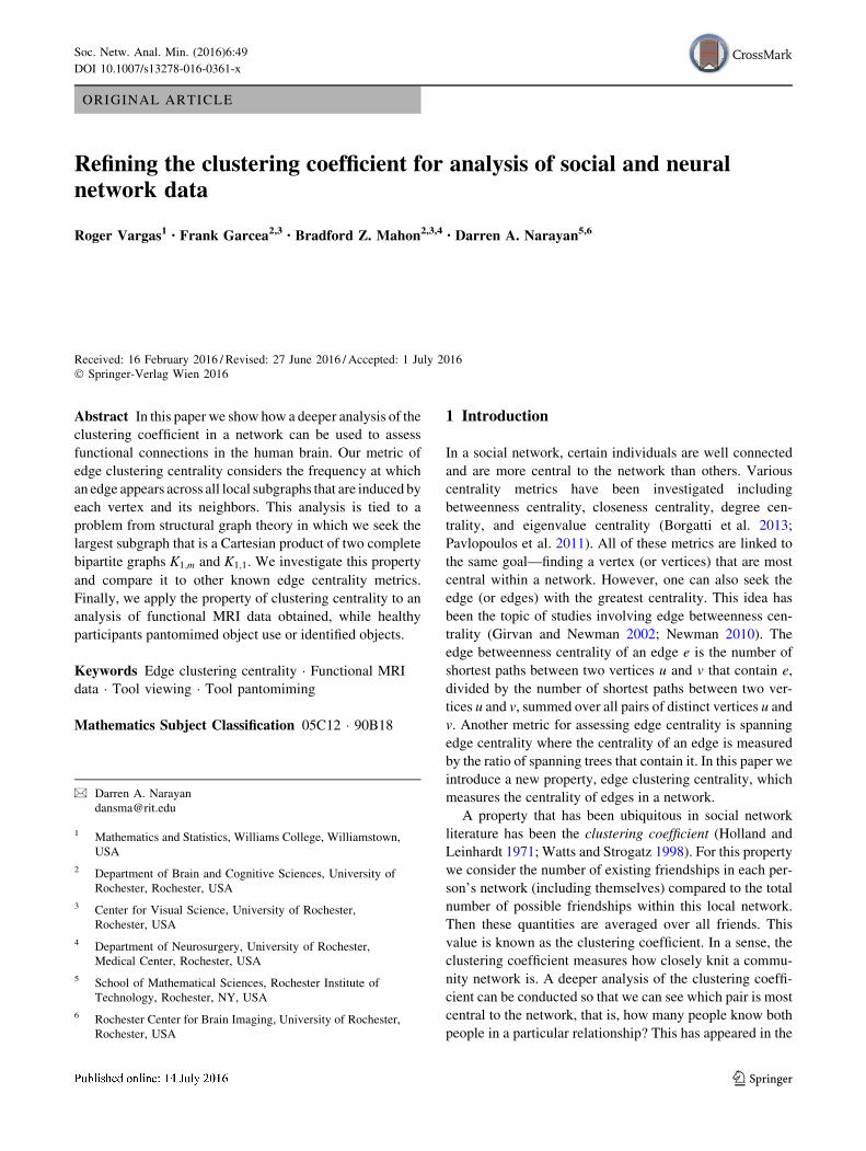
We consider the following example (Fig. 2).
The local subgraphs are as follows (Fig. 3).
For each of the cases, we calculate the number of edges in
the local subgraph compared to the number of possible
edges: GA : 3=3, GB : 8=10, GC : 6=6, GD : 6=6, and
GE : 8=10. The closed clustering coefficient is the average of
these fractions: CCðGÞ ¼ 151þ 0:8þ 1þ 1þ 0:8ð Þ ¼ 0:92.
This high value indicates that the graph is highly connected;
however, this single number does not capture some of the
finer aspects of this network.
By seeking edges that appear in multiple local sub-
graphs, we can identify edges that are more important to
the network as a whole. We start by combining all of the
local subgraphs (counting multiplicities) into a single graph
TG. The result is shown in Fig. 4.
This idea forms the cases for a new measure which we
will call edge clustering centrality. The edge clustering
centrality of an edge is CcentðeÞ ¼X
ifiðeÞ where fiðeÞ ¼ 1
if e 2 E Gið Þ and fiðeÞ ¼ 0 if e 62 E Gið Þ and Gi is the closed
Fig. 1 A wedding network with darker edges showing people
connected to both the bride and groom
Fig. 2 A graph with 5 vertices
and 8 edges
Fig. 3 The local subgraphs of G
Fig. 4 Combination of local
subgraphs
49 Page 2 of 8 Soc. Netw. Anal. Min. (2016) 6:49
123
neighborhood of vertex i. In our example, CcentðEBÞ ¼ 5,
CcentðBCÞ ¼ CcentðBDÞ ¼ CcentðCDÞ ¼ CcentðCEÞ ¼CcentðDEÞ ¼ 4, and CcentðAEÞ ¼ CcentðABÞ ¼ 3. Since EB
has the highest clustering centrality, it can be considered
more important to the network’s connectivity, whereas
edges AB and AE can be considered of lesser importance.
In this paper we will explore the property of clustering
centrality. We first show it can be formulated as a problem
in structural graph theory. Next we show how it differs
from other centrality metrics, and finally we apply it to a
real-world problem involving the analysis of functional
connectivity of the human brain.
2 Edge clustering centrality
Computing the frequencies that edges appear across all
local subgraphs is straightforward. The problem of finding
the edge with the greatest frequency can be linked to a
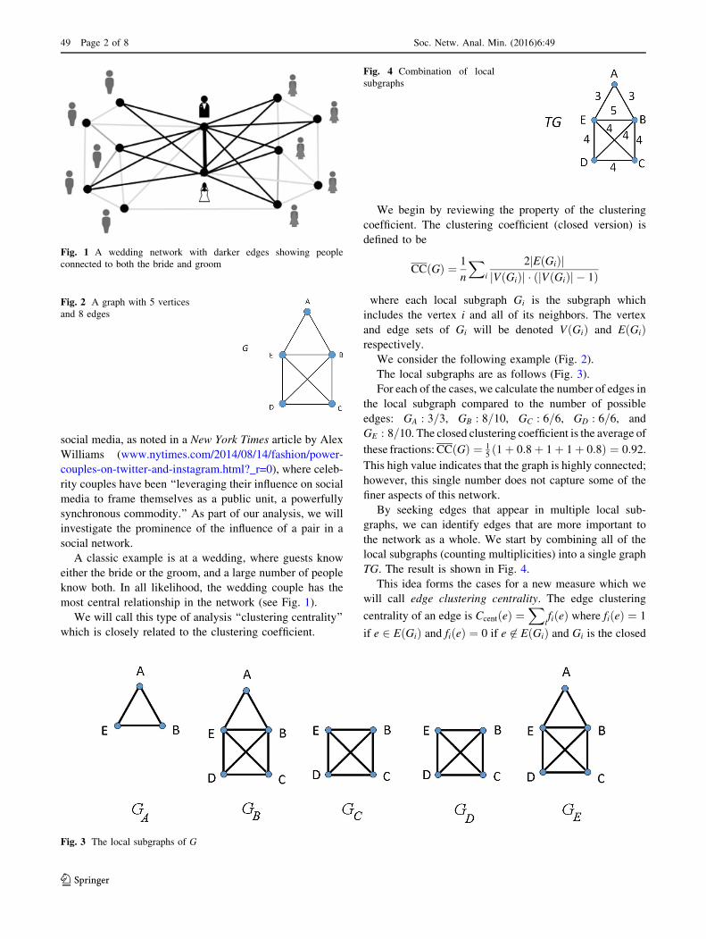
problem in extremal graph theory. The graph shown in
Fig. 5 is an example of a Cartesian Product of two com-
plete bipartite graphs K1;m and K1;1 and is known as a book
graph Bm (with K1;1 serving as the ‘‘spine’’) (Sun 1994;
Liang 1997; Barioli 1998; Shi and Song 2007) and has
been a focus of studies in Graph Ramsey Theory
(Radziszowski et al. 2014). In our analysis, we will search
for the maximum sized book graph H found in a graph
G. The spine of the graph H will have the highest edge
clustering centrality of any edge in G.
We note that the edge clustering centrality of an edge e
in a graph G can be computed simply by counting the
number of triangles in G containing e—a computation for
which efficient algorithms exist. Looking back to the
wedding example in Fig. 1, the darker edges correspond to
the book graph B6.
2.1 Comparison with other edge centrality
properties
We next show that edge clustering centrality differs from
other known edge centrality metrics, including edge
betweenness centrality, j-path centrality, and spanning
edge centrality. The most well-known edge centrality
property is edge betweenness centrality introduced by
Freeman (1977) and later used in modularity algorithms by
Girvan and Newman (2002) and Newman (2010).
Definition 1 The edge betweenness centrality of an edge
e, denoted bc(e), measures the frequency at which e
appears on a shortest path between two distinct vertices x
and y. Let rxy be the number of shortest paths between
distinct vertices x and y, and let rxyðeÞ be the number of
shortest paths between x and y that contain e. Then bcðeÞ ¼X
x;y
rxyðeÞrxy
(for all distinct vertices x, and y).
Edge clustering centrality works especially well in
dense graphs; however, sparse graphs may have edges
that are not contained in any triangles and thus these
edges will have an edge clustering centrality of zero.
Hence, for sparse graphs such as paths or cycles, edge
betweenness centrality would be preferable to use. How-
ever, this may not be true for dense graphs. We will show
in the next example if the graph contains a book graph as
a subgraph, edge clustering centrality can give a better
measure of edge centrality.
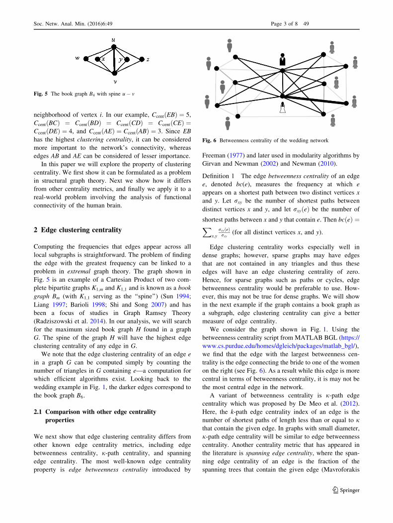
We consider the graph shown in Fig. 1. Using the
betweenness centrality script from MATLAB BGL (https://
www.cs.purdue.edu/homes/dgleich/packages/matlab_bgl/),
we find that the edge with the largest betweenness cen-
trality is the edge connecting the bride to one of the women
on the right (see Fig. 6). As a result while this edge is more
central in terms of betweenness centrality, it is may not be
the most central edge in the network.
A variant of betweenness centrality is j-path edge
centrality which was proposed by De Meo et al. (2012).
Here, the k-path edge centrality index of an edge is the
number of shortest paths of length less than or equal to jthat contain the given edge. In graphs with small diameter,
j-path edge centrality will be similar to edge betweenness
centrality. Another centrality metric that has appeared in
the literature is spanning edge centrality, where the span-
ning edge centrality of an edge is the fraction of the
spanning trees that contain the given edge (Mavroforakis
Fig. 5 The book graph B4 with spine u� v
Fig. 6 Betweenness centrality of the wedding network
Soc. Netw. Anal. Min. (2016) 6:49 Page 3 of 8 49
123
et al. 2015). However this metric is only applicable for
graphs that are connected. Furthermore, there can be con-
cerns if a graph contains a pendant edge (an edge incident
to a vertex with degree one). A pendant edge will typically
not be central to the graph, but it will have a high spanning
edge centrality (consistent with any cut-edge) since it will
appear in every spanning tree.
3 A real-world application
We will use centrality metrics from graph theory to model
brain connectivity. In our graph model, the vertices cor-
respond to physical regions of the brain [Regions of
Interest (ROIs)], and the undirected edges correspond to a
correlation in the functional activation profiles associated
with the two vertices. Functional Magnetic Resonance data
(fMRI) consist of a time course of Blood Oxygenated
Level Dependent (BOLD) contrast (activation) for every
voxel in space. Hence, an undirected edge is present in two
regions of the brain if there is a strong correlation between
the time series of BOLD signals between the respective
regions.
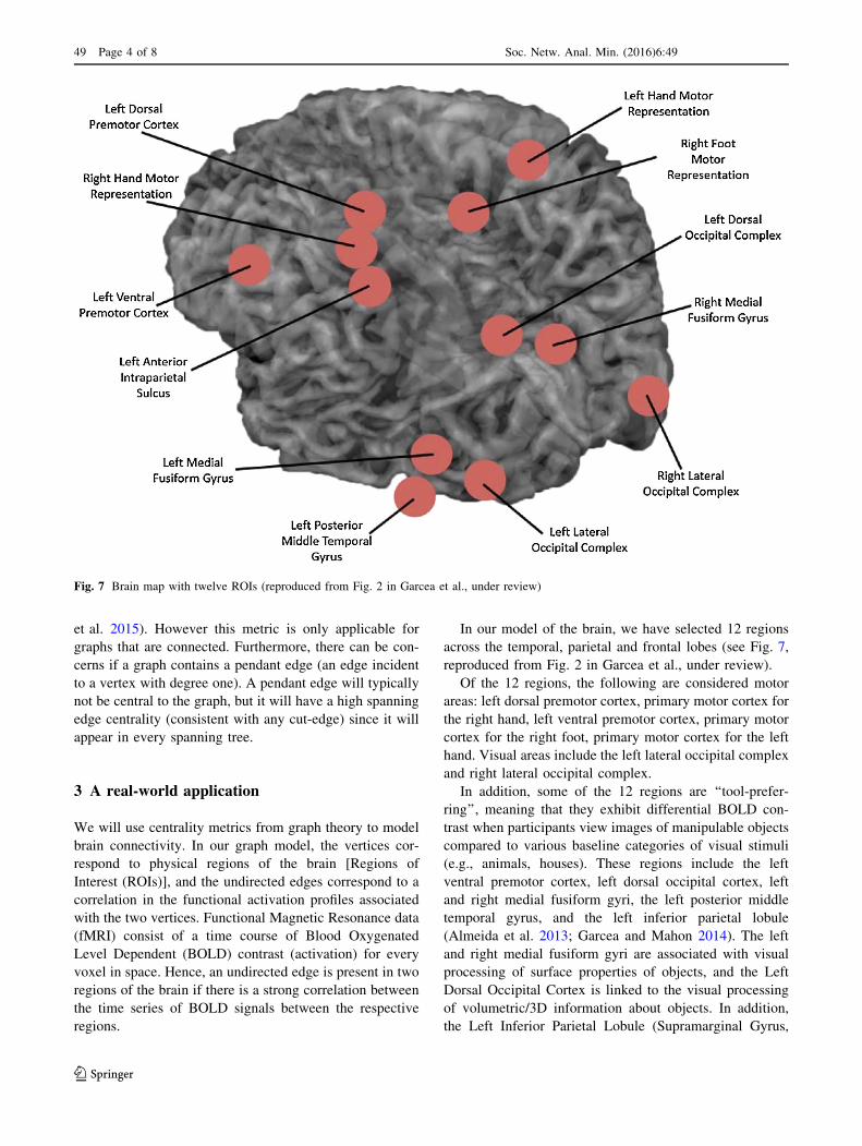
In our model of the brain, we have selected 12 regions
across the temporal, parietal and frontal lobes (see Fig. 7,
reproduced from Fig. 2 in Garcea et al., under review).
Of the 12 regions, the following are considered motor
areas: left dorsal premotor cortex, primary motor cortex for
the right hand, left ventral premotor cortex, primary motor
cortex for the right foot, primary motor cortex for the left
hand. Visual areas include the left lateral occipital complex
and right lateral occipital complex.
In addition, some of the 12 regions are ‘‘tool-prefer-
ring’’, meaning that they exhibit differential BOLD con-
trast when participants view images of manipulable objects
compared to various baseline categories of visual stimuli
(e.g., animals, houses). These regions include the left
ventral premotor cortex, left dorsal occipital cortex, left
and right medial fusiform gyri, the left posterior middle
temporal gyrus, and the left inferior parietal lobule
(Almeida et al. 2013; Garcea and Mahon 2014). The left
and right medial fusiform gyri are associated with visual
processing of surface properties of objects, and the Left
Dorsal Occipital Cortex is linked to the visual processing
of volumetric/3D information about objects. In addition,
the Left Inferior Parietal Lobule (Supramarginal Gyrus,
Fig. 7 Brain map with twelve ROIs (reproduced from Fig. 2 in Garcea et al., under review)
49 Page 4 of 8 Soc. Netw. Anal. Min. (2016) 6:49
123
Anterior Intraparietal Sulcus) is a region that is important
for representing manipulation knowledge (i.e., the knowl-
edge of how to correctly grasp and manipulate an object).
The dataset used in this paper was collected at the
Rochester Center for Brain Imaging (University of
Rochester) with 12 healthy, right-handed individuals (for
full details of the experimental paradigm, MRI acquisition,
preprocessing, and analysis, see Garcea et al., under
review). Data were collected in two different tasks in
which participants were shown images of various tools:
hammer, scissors, screwdriver, knife, pliers, and cork-
screw. In one task, participants were asked to pantomime
the use of a presented object with their right hand during
the fMRI, while during the second task participants were
asked to and identify the images.
We looked at correlations in BOLD time series between
each pair of 12 different regions. A two tailed t test was
performed, and statistically significant values (at t[ 2:75 )
were selected. For each pair of regions, the temporal corre-
lations in BOLD time series were computed separately for
the task in which participants were pantomiming the object
use and identifying the objects. The data consisted of two
12� 12 correlation matrices for each subjects (one matrix
for pantomiming and one for viewing). These matrices were
subtracted from one another to create two matrices, one
where pantomiming was greater than visual, and a second
where the visual was larger than pantomiming.
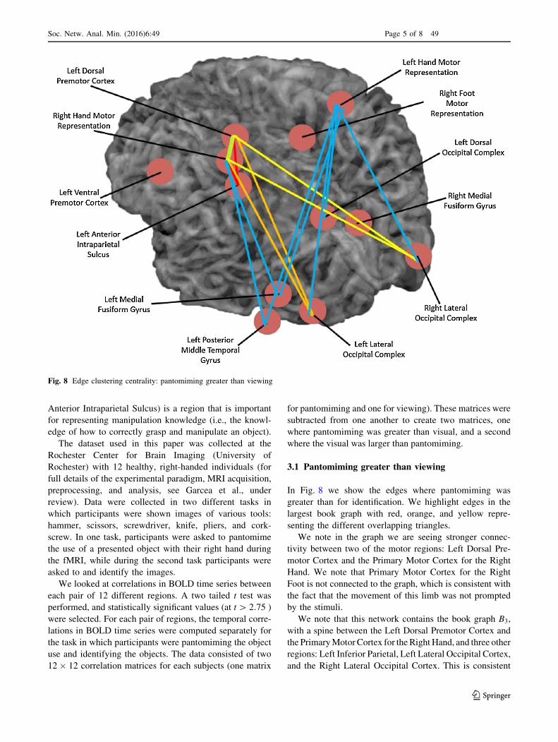
3.1 Pantomiming greater than viewing
In Fig. 8 we show the edges where pantomiming was
greater than for identification. We highlight edges in the
largest book graph with red, orange, and yellow repre-
senting the different overlapping triangles.
We note in the graph we are seeing stronger connec-
tivity between two of the motor regions: Left Dorsal Pre-
motor Cortex and the Primary Motor Cortex for the Right
Hand. We note that Primary Motor Cortex for the Right
Foot is not connected to the graph, which is consistent with
the fact that the movement of this limb was not prompted
by the stimuli.
We note that this network contains the book graph B3,
with a spine between the Left Dorsal Premotor Cortex and
the PrimaryMotor Cortex for the Right Hand, and three other
regions: Left Inferior Parietal, Left Lateral Occipital Cortex,
and the Right Lateral Occipital Cortex. This is consistent
Fig. 8 Edge clustering centrality: pantomiming greater than viewing
Soc. Netw. Anal. Min. (2016) 6:49 Page 5 of 8 49
123
with neurological expectations as these three ’are involved in
accessing object-directed manipulation knowledge from the
visual structure of objects (for details and discussion, see
Garcea et al., under review). Furthermore, the result that the
Left Dorsal Premotor Cortex is on the spine of the graph is
consistent with the fact that both of this motor region is part
of the tool network (Garcea and Mahon 2014). Although the
Left and Right Lateral Occipital Cortex regions are associ-
ated with visual object recognition, there is connectivity
between each of them and the motor regions on the book
spine. The reason for this is that in order to pantomime a tool,
there has to be a connection among visual regions first (as the
subject recognizes the tool) and then a connection between
motor regions as the tool is manipulated (Almeida et al.
2013; Mahon et al. 2013).
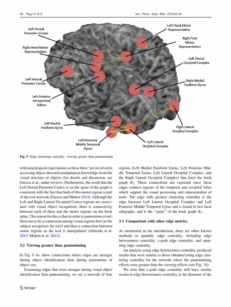
3.2 Viewing greater than pantomiming
In Fig. 9 we show connections where edges are stronger
during object identification then during pantomime of
object use.
Examining edges that were stronger during visual object
identification than pantomiming, we see a network of four
regions (Left Medial Fusiform Gyrus, Left Posterior Mid-
dle Temporal Gyrus, Left Lateral Occipital Complex, and
the Right Lateral Occipital Complex) that form the book
graph B2. These connections are expected since these
edges connect regions of the temporal and occipital lobes
which support the visual processing and representation of
tools. The edge with greatest clustering centrality is the
edge between Left Lateral Occipital Complex and Left
Posterior Middle Temporal Gyrus and is found in two local
subgraphs, and is the ‘‘spine’’ of the book graph B2.
3.3 Comparison with other edge metrics
As mentioned in the introduction, there are other known
methods to quantify edge centrality, including edge
betweenness centrality, j-path edge centrality, and span-
ning edge centrality.
An analysis using edge betweenness centrality produced
results that were similar to those obtained using edge clus-
tering centrality for the network where the pantomiming
effects were greater than the viewing effects (see Fig. 10).
We note that j-path edge centrality will have similar
results to edge betweenness centrality as the diameter of the
Fig. 9 Edge clustering centrality: viewing greater than pantomiming
49 Page 6 of 8 Soc. Netw. Anal. Min. (2016) 6:49
123
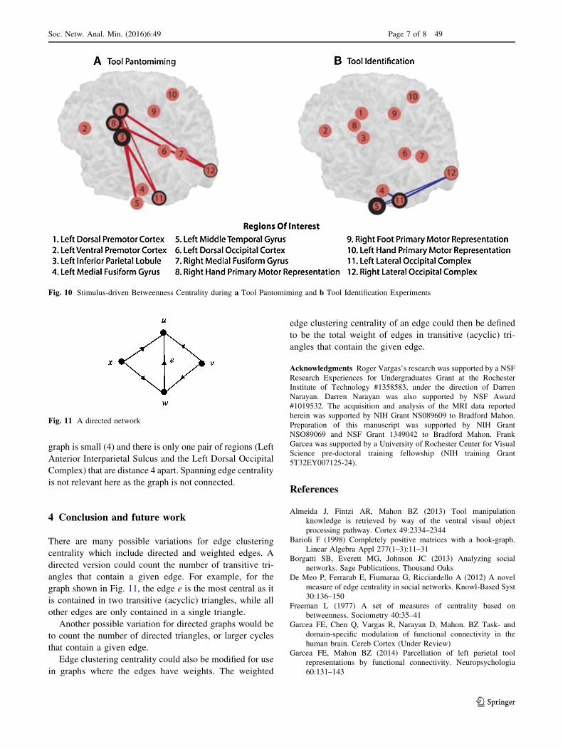
graph is small (4) and there is only one pair of regions (Left
Anterior Interparietal Sulcus and the Left Dorsal Occipital
Complex) that are distance 4 apart. Spanning edge centrality
is not relevant here as the graph is not connected.
4 Conclusion and future work
There are many possible variations for edge clustering
centrality which include directed and weighted edges. A
directed version could count the number of transitive tri-
angles that contain a given edge. For example, for the
graph shown in Fig. 11, the edge e is the most central as it
is contained in two transitive (acyclic) triangles, while all
other edges are only contained in a single triangle.
Another possible variation for directed graphs would be
to count the number of directed triangles, or larger cycles
that contain a given edge.
Edge clustering centrality could also be modified for use
in graphs where the edges have weights. The weighted
edge clustering centrality of an edge could then be defined
to be the total weight of edges in transitive (acyclic) tri-
angles that contain the given edge.
Acknowledgments Roger Vargas’s research was supported by a NSF
Research Experiences for Undergraduates Grant at the Rochester
Institute of Technology #1358583, under the direction of Darren
Narayan. Darren Narayan was also supported by NSF Award
#1019532. The acquisition and analysis of the MRI data reported
herein was supported by NIH Grant NS089609 to Bradford Mahon.
Preparation of this manuscript was supported by NIH Grant
NSO89069 and NSF Grant 1349042 to Bradford Mahon. Frank
Garcea was supported by a University of Rochester Center for Visual
Science pre-doctoral training fellowship (NIH training Grant
5T32EY007125-24).
References
Almeida J, Fintzi AR, Mahon BZ (2013) Tool manipulation
knowledge is retrieved by way of the ventral visual object
processing pathway. Cortex 49:2334–2344
Barioli F (1998) Completely positive matrices with a book-graph.
Linear Algebra Appl 277(1–3):11–31
Borgatti SB, Everett MG, Johnson JC (2013) Analyzing social
networks. Sage Publications, Thousand Oaks
De Meo P, Ferrarab E, Fiumaraa G, Ricciardello A (2012) A novel
measure of edge centrality in social networks. Knowl-Based Syst
30:136–150
Freeman L (1977) A set of measures of centrality based on
betweenness. Sociometry 40:35–41
Garcea FE, Chen Q, Vargas R, Narayan D, Mahon. BZ Task- and
domain-specific modulation of functional connectivity in the
human brain. Cereb Cortex (Under Review)
Garcea FE, Mahon BZ (2014) Parcellation of left parietal tool
representations by functional connectivity. Neuropsychologia
60:131–143
Fig. 10 Stimulus-driven Betweenness Centrality during a Tool Pantomiming and b Tool Identification Experiments
Fig. 11 A directed network
Soc. Netw. Anal. Min. (2016) 6:49 Page 7 of 8 49
123
Girvan M, Newman MEJ (2002) Community structure in social and
biological networks. Proc Natl Acad Sci USA 99:7821–7826
Holland PW, Leinhardt S (1971) Transitivity in structural models of
small groups. Comp Group Stud 2:107–124
Liang Z (1997) The harmoniousness of book graph Stð4k þ 1Þ � P2.
Southeast Asian Bull Math 21(2):181–184
Mahon BZ, Kumar N, Almeida J (2013) Spatial frequency tuning
reveals interactions between the dorsal and ventral visual
systems. J Cogn Neurosci 25:862–871
Mavroforakis C, Garcia-Lebron R, Koutis I, Terzi E (2015) Spanning
edge centrality: large-scale computation and applications, ACM
978-1-4503-3469-3/15/05. doi:10.1145/2736277.2741125
MatlabBGL. https://www.cs.purdue.edu/homes/dgleich/packages/
matlab_bgl/
Newman MEJ (2010) Networks: an introduction. Oxford University
Press, Oxford
Pavlopoulos GA, Secrier M, Moschopoulos CN, Soldatos TG,
Kossida S, Aerts J, Schneider R, Bagos PG (2011) Using graph
theory to analyze biological networks. BioData Min 4:10. doi:10.
1186/1756-0381-4-10
Radziszowski S (2014) Small Ramsey numbers, Dynamic Survey
#DS1. Electron J Comb
Shi L, Song Z (2007) Upper bounds on the spectral radius of book-
free and/or K2, l-free graphs. Linear Algebra Appl 420:526–529
Sun RG (1994) Harmonious and sequential labelings of the book
graphs Bm. (Chinese). Gaoxiao Yingyong Shuxue Xuebao Ser A
9(3):335–337
The Power of Two; Power Couples on Twitter and Instagram. www.
nytimes.com/2014/08/14/fashion/power-couples-on-twitter-and-
instagram.html?_r=0
Watts DJ, Strogatz SH (1998) Collective dynamics of ‘small-world’
networks. Nature 393(6684):440–442
49 Page 8 of 8 Soc. Netw. Anal. Min. (2016) 6:49
123