PNNL-20754

Prepared for the U.S. Department of Energy under Contract DE-AC05-76RL01830

Renewable Energy Requirements for Future Building Codes: Energy Generation and Economic Analysis BJ Russo MR Weimar HE Dillon September 2011

PNNL-20754

Renewable Energy Requirements for Future Building Codes: Energy Generation and Economic Analysis BJ Russo MR Weimer HE Dillon September 2011 Prepared for the U.S. Department of Energy under Contract DE-AC05-76RL01830 Pacific Northwest National Laboratory Richland, Washington 99352

iii

v

Summary

As the model energy codes are improved to reach efficiency levels 50 percent greater than current codes, installation of on-site renewable energy generation is likely to become a code requirement. This requirement will be needed because traditional mechanisms for code improvement, including the building envelope, mechanical systems, and lighting, have been maximized at the most cost-effective limit. Research has been conducted to determine the mechanism for implementing this requirement (Kaufman 2011). Kaufmann et al. determined that the most appropriate way to structure an on-site renewable requirement for commercial buildings is to define the requirement in terms of an installed power density per unit of roof area. This provides a mechanism that is suitable for the installation of photovoltaic (PV) systems on future buildings to offset electricity and reduce the total building energy load. Kaufmann et al. suggested that an appropriate maximum for the requirement in the commercial sector would be 4 W/ft2 of roof area or 0.5 W/ft2 of conditioned floor area. This research expands on the work of Kaufman to develop possible requirements levels for residential buildings and refines the estimates from Kaufman. A simple economic analysis has been performed to determine reasonable cost effectiveness for future PV requirements. Section 1 of the report provides background and a summary of prior work. Section 2 provides an overview of the simulation methodology applied in this work. Section 3 provides results for the PV array modeling efforts, with detailed results shown in Appendix A. Section 4 gives the details used for the economic analysis and summarizes the conclusions. Several important conclusions are possible based on this analysis work:

• It is reasonable to consider a higher on-site renewable generation requirement for commercial buildings than that proposed by Kaufman et al. (Kaufman 2011). This analysis indicates 6 watts/sf as a nationwide average, with possible exceptions for specific building types.

• The on-site renewable generation requirement for residential buildings should be 4 watts/sf based on a national average.

• The breakeven cost of electricity produced by a commercial PV array is $0.20-0.22/kWh using a 3% IRR.

• The breakeven cost of electricity produced by a residential PV array is $0.29/kWh using a 3% IRR.

vii

Acronyms and Abbreviations

AEO Annual Energy Outlook ANSI American National Standards Institute ASHRAE American Society of Heating, Refrigerating and Air-Conditioning Engineers DOE Department of Energy EIA Energy Information Administration HVAC Heating, Ventilation and Air Conditioning ICC International Code Council IECC International Energy Conservation Code PNNL Pacific Northwest National Laboratory PV Photovoltaic REC Renewable Energy Credit

ix

Contents

Summary .............................................................................................................................................. v  Acronyms and Abbreviations ........................................................................................................... vii  1.0   Background .............................................................................................................................. 1.1  2.0   Optimization Methodology ...................................................................................................... 2.2  3.0   Photovoltaic Array Modeling Results ...................................................................................... 3.6  4.0   Economic Analysis ................................................................................................................... 4.9  5.0   Conclusions and Recommendations ...................................................................................... 5.14  6.0   References .............................................................................................................................. 6.15  Appendix A: Detailed Results of PV Array Installed Capacity Scenarios ..................................... 6.16  

1.1

1.0 Background

Current model energy codes like the International Energy Conservation Code (IECC) and ASHRAE Standard 90.1 do not have prescriptive requirements for onsite renewable energy systems. Recently, some codes and standards have included requirements for onsite renewable energy generation systems. ASHRAE Standard 189.1, Standard for the Design of High-Performance Green Buildings, the city of Seattle, Washington, and the IGCC (International Green Construction Code) all represent examples of this process as it develops in the energy codes. The existing codes are discussed in more detail in other technical reports including Kaufmann et al (Kaufmann 2011) and Dillon et al (Dillon 2011). Research has been conducted to determine the mechanism for implementing a future renewable energy generation requirement (Kaufman 2011). Kaufmann et al. determined that the most appropriate way to structure an on-site renewable requirement for commercial buildings is to define the requirement in terms of an installed power density per unit of roof area. This provides a mechanism that is suitable for the installation of photovoltaic (PV) systems on future buildings to offset electricity and reduce the total building energy load. Kaufmann et al. suggested that an appropriate maximum for the requirement in the commercial sector would be 4 W/ft2 of roof area or 0.5 W/ft2 of conditioned floor area. As with all code requirements, there must be an alternative compliance path for buildings that may not reasonably meet the renewables requirement. This might include conditions like shading (which makes rooftop PV arrays less effective), unusual architecture, undesirable roof pitch, unsuitable building orientation, or other issues. The methodology for determining alternative compliance paths based on Renewable Energy Credits (RECs) was developed by Dillon et al (Dillon 2011). Kaufmann did not consider the most appropriate level of renewable energy generation for the residential market, and did not optimize the results developed for the commercial market. In addition to this analytical need, an economic analysis of the requirement is needed to provide a basis for cost effective energy code development. This work provides the next iteration of the preliminary calculations from Kaufman et al. The following items are addressed:

• Further optimization of the Kaufman analysis for commercial buildings with additional technical detail.

• Initial determination of the most appropriate requirement level for residential buildings. • Economic analysis of the possible renewable energy generation requirement if onsite PV arrays

are used for compliance.

2.2

2.0 Optimization Methodology

Integration of renewable energy requirements into building codes can be challenging given the nation’s wide range of building types, renewable resource availability, and the volume of buildings available for integrated renewable energy systems. In this high-level analysis, the potential for renewable energy development at commercial and residential buildings was estimated by modeling the performance of roof-mounted photovoltaic (PV) arrays with Canada’s Natural Resource RETScreen program. Table 1 documents the details of the modules and arrays modeled in this analysis. These parameters were selected as they represent a typical system available on the market.

Table 1: PV Module Details

Characteristic Module Polycrystalline silicon Module Efficiency 13% Temperature Coefficient 0.4%/°C Dimensions 3.3 x 4.9 x 0.16 ft Module Wattage 200 watts

To perform this analysis, the output of arrays installed on the IECC prototype residence (DOE 2011) and the 16 ASHREA 90.1 prototype commercial buildings were modeled. PV array performance was modeled assuming flush mounting on a flat roof (i.e., 0° tilt) modules as this is common practice for commercial building roofs with PV arrays.1 Prototype buildings for the fast food restaurant, sit-down restaurant, and small office have tilted roofs and thus only the south-facing, tilted roof portion was assumed to be available for an array. Additionally, the IECC prototype home features a hip roof; therefore, it was assumed that only the south-facing portion would be available for array siting. Lastly, it was assumed that in the case of buildings with pitched roofs, the roof exposure suitable for an array was oriented to face south. Most commercial building roofs are populated with structures and features such as penthouses, rooftop HVAC equipment, vents, parapet walls, etc. These structures limit the amount of roof area available for an array. During the installation of an array, open area must also be preserved to maintain access corridors and pathways for the purposes of building and equipment maintenance (e.g., HVAC units, PV modules and wiring, etc.) and for fire suppression efforts in the case of a fire. Consequently, it was assumed that 50% of the roof area would be available for an array in the case of commercial buildings. Residential homes typically have far fewer roof penetrations and structures and therefore it was assumed that 70% of the suitable roof area would be available for an array. Table 2 provides the relevant details of these prototype buildings.

1 Tilted arrays are also installed on flat roofs, although in these cases the module tilt is either relatively minor or notable amounts of space must be preserved between module strings to avoid self-shading.

2.3

Table 2: Prototype Building Details

Building Building Type

Interior Area

sf

Site Energy

Use Intensity, kWh/sf2

Site Energy

Use, kWh3

Total Roof Space,

sf

Roof Pitch,

degrees

High rise Apartment Commercial 75,966 13 979,586 8,436 0.0 Hospital Commercial 241,411 55 13,195,003 40,250 0.0 Large Hotel Commercial 122,072 61 7,459,261 15,904 0.0 Large Office Commercial 498,403 13 6,704,501 38,400 0.0 Medium Office Commercial 53,606 14 743,105 17,876 0.0 Midrise Apartment Commercial 30,386 13 387,382 8,436 0.0 Outpatient Health Care Commercial 40,931 44 1,813,750 14,319 0.0

Primary School Commercial 73,932 20 1,512,379 73,440 0.0 Retail Stripmall Commercial 22,488 22 496,939 22,500 0.0 Secondary School Commercial 210,810 21 4,349,473 130,944 0.0 Small Hotel Commercial 43,180 20 875,710 10,800 0.0 Stand-alone Retail Commercial 24,683 21 515,061 24,742 0.0 Fast Food Restaurant Commercial 2,496 164 408,159 1,250 18.4

Sit Down Restaurant Commercial 5,498 114 626,355 2,738 18.4

Small Office Commercial 5,498 12 64,456 2,753 18.4 Residential Home Residential 2,400 11 26,620 1,389 16.7

As previously stated, PV array performance was modeled with RETScreen. PV array output was normalized to a kilowatt-hour per square foot performance that could then be extrapolated to the available open roof area. To estimate the performance of the arrays across the United States, six cities were selected from those used in the ASHREA 90.1-2004 code development effort as representative cities spanning the typical insolation range of the continental U.S. These cities are selected based on their location within the major climate zones in the US. However, these climate zones are primarily defined by heating degree days, cooling degree days, and typical precipitation/moisture patterns, and not by insolation levels (for instance, despite being located in climate zone five, Boise receives more insolation than any other location within climate zone five aside from El Paso). Therefore, it was not necessary to determine a representative city for all climate zones. Figure 1 provides a map of the insolation levels in the US. Table 3 documents the selected cities.

2 For the residential building, this value reflects an average value weighted by building starts across all climate zones and HVAC and domestic water heating technology combinations from the 2006 IECC. 3 For the residential building, this value reflects an average value weighted by building starts across all climate zones and HVAC and domestic water heating technology combinations from the 2006 IECC.

2.4

Figure 1. Insolation for Flat-Plate Collectors at Latitude Tilt. In other words, a flat collector (rather than a curved concentrating collector) tilted at each site’s latitude (NREL 2011)

Table 3: PV Module Details City Climate Zone Latitude and Longitude Annual Horizontal Insolation, kWh/m2/day

El Paso 3 31.8, -106.4 5.33

Memphis 3 35.1, -90.0 4.24

Baltimore 3 39.3, -76.6 3.70

Salem 4 44.9, -123.0 3.73

Boise 5 43.6, -116.2 4.45

Burlington 6 44.8, -73.2 3.49

After modeling the arrays’ performance, the arrays’ energy production was evaluated against the buildings’ gross energy consumption. The maximum install density potential was determined by modeling an array that occupies the maximum amount of available roof space. If this resulted in an array that produces more energy than is consumed by a building, the array was limited in scale to produce no more than 100% of a building’s total energy demand. However, this limit was only required in a small number of cases for buildings in sunny areas with large roofs and a low energy use intensity (EUI). Additional runs were conducted to explore the effect of limiting the array’s scale to meet a smaller fraction of a building’s total energy load.

2.5

This analysis assumed that all installed arrays are capable of participating in a net metering program. Net metering programs allow excess electricity to be exported to the local grid when the array is producing more electricity than a building requires. In the case of residential buildings, likely periods of excess production are during the weekday daytimes when the building may be largely unoccupied. For commercial buildings, excess may occur during weekends if the building is unoccupied. In both building types, an array may produce excess electricity during particularly sunny days when array output is maximized. In locations where net metering is unavailable or when governmentally established net metering limits have been met (e.g., a net metering fraction to be no larger than 10% of a utility’s aggregated capacity or sales), excess generation will need to be shunted or portions of the array will need to be brought off-line. Under these conditions, excess generation or potential generation cannot be counted towards reducing a building’s gross energy demand. As a result, it may be challenging for buildings in these circumstances to employ on-site renewable energy generation as a means to reduce their total energy demand or meet a code requiring on-site renewable energy generation. This issue may require additional analysis prior to code language development.

3.6

3.0  Photovoltaic Array Modeling Results

System electrical and economic performance was analyzed to help establish physical and economic bounds for building-integrated renewable energy systems during building code development.

Table 4 documents the performance of the arrays at the six selected cities and three prototype building rooftop types. Specifically, the table documents the capacity factor and electricity production per installed kilowatt of each PV array. The capacity factor is a measure of the productivity of a kilowatt of a power system; a system that is available all hours and days of the year (i.e., 8,760 hours per year) has a capacity factor of 100%. As shown in Table 4:

• Cities located in more southerly and arid locations have superior PV array performance over cites located in northerly and cloudy locations.

• Arrays on tilted rooftops are more optimally oriented to capture insolation and thus have better capacity factors.

• The average system performance across the six locations on each roof type (weighted by building starts) is provided. Building starts data was obtained from the “An Estimate of Residential Energy Savings from IECC Change Proposals Recommended for Approval at the ICC’s Fall, 2009, Initial Action Hearings” 2010 report (Taylor 2010).

Table 4: PV Array Performance by Location and Roof Type

City

Capacity Factors PV Array Electricity Production, kWhac per Installed kW

Flat Roof Tilted Roof

(18.4°)

Residential Hip Roof

(16.7°) Flat Roof

Tilted Roof

(18.4°)

Residential Hip Roof

(16.7°) El Paso 14.3% 15.4% 15.3% 1,857 2,006 1,997

Memphis 16.9% 18.7% 18.6% 1,489 1,594 1,594

Baltimore 14.6% 16.2% 16.1% 1,253 1,349 1,340

Salem 21.2% 22.9% 22.8% 1,253 1,367 1,358

Boise 17.0% 18.2% 18.2% 1,480 1,638 1,629

Burlington 14.3% 15.6% 15.5% 1,279 1,419 1,410 Average Performance (weighted by building starts)

16.5% 17.9% 17.8% 1,448 1,564 1,558

Table 5 documents the PV array maximum install density in watts per square foot of total roof area. Appendix A presents this information in greater detail and documents the array capacity in kilowatts, the array output in kilowatt-hours, and the percent of the total building energy load displaced by solar electricity. To further explore the impact of install density relative to the total building energy consumption, three different scenarios were considered:

3.7

• Scenario 1: arrays were sized to occupy 100% of the roof space, provided an array’s output does not exceed 100% of a building’s total energy load. If an array’s output exceeds the total energy load, the array was sized to meet 100% of the building’s annual energy load.

• Scenario 2: arrays were sized to meet 50% of a building’s annual energy load. If the load cannot be met with the available roof space, arrays were sized to occupy 100% of the available roof space.

• Scenario 3: arrays were sized to meet 10% of a building’s annual energy load. If the load cannot be met with the available roof space, arrays were sized to occupy 100% of the available roof space.

Table 5: PV Array Install Density (W/sf) by Building Type and Location* Building Type HA HO LH LO MO MA OP PS RF RS SS SR SH SO SA W RH

Scenario 1: Arrays Sized to Meet 100% Energy Load if Roof Space is Available (w/sf) El Paso 6.3 6.3 6.3 6.3 6.3 6.3 6.3 6.3 3.3 6.3 6.3 4.2 6.3 4.2 6.3 4.6 4.0 Boise 6.3 6.3 6.3 6.3 6.3 6.3 6.3 6.3 3.3 6.3 6.3 4.2 6.3 4.2 6.3 5.4 4.0 Memphis 6.3 6.3 6.3 6.3 6.3 6.3 6.3 6.3 3.3 6.3 6.3 4.2 6.3 4.2 6.3 5.7 4.0 Salem 6.3 6.3 6.3 6.3 6.3 6.3 6.3 6.3 3.3 6.3 6.3 4.2 6.3 4.2 6.3 6.3 4.0 Baltimore 6.3 6.3 6.3 6.3 6.3 6.3 6.3 6.3 3.3 6.3 6.3 4.2 6.3 4.2 6.3 6.3 4.0 Burlington 6.3 6.3 6.3 6.3 6.3 6.3 6.3 6.3 3.3 6.3 6.3 4.2 6.3 4.2 6.3 6.3 4.0

Scenario 2: Arrays Sized to Meet 50% Energy Load if Roof Space is Available (w/sf) El Paso 6.3 6.3 6.3 6.3 6.3 6.3 6.3 5.9 3.3 6.3 6.3 4.2 6.3 4.2 6.0 2.3 3.8 Boise 6.3 6.3 6.3 6.3 6.3 6.3 6.3 6.3 3.3 6.3 6.3 4.2 6.3 4.2 6.3 2.7 4.0 Memphis 6.3 6.3 6.3 6.3 6.3 6.3 6.3 6.3 3.3 6.3 6.3 4.2 6.3 4.2 6.3 2.9 4.0 Salem 6.3 6.3 6.3 6.3 6.3 6.3 6.3 6.3 3.3 6.3 6.3 4.2 6.3 4.2 6.3 3.2 4.0 Baltimore 6.3 6.3 6.3 6.3 6.3 6.3 6.3 6.3 3.3 6.3 6.3 4.2 6.3 4.2 6.3 3.2 4.0 Burlington 6.3 6.3 6.3 6.3 6.3 6.3 6.3 6.3 3.3 6.3 6.3 4.2 6.3 4.2 6.3 3.3 4.0

Scenario 3: Arrays Sized to Meet 10% Energy Load if Roof Space is Available (w/sf) El Paso 6.3 6.3 6.3 6.3 2.4 2.6 6.3 1.2 3.3 1.3 1.9 4.2 4.7 1.2 1.2 0.5 0.8 Boise 6.3 6.3 6.3 6.3 2.8 3.1 6.3 1.4 3.3 1.5 2.2 4.2 5.4 1.4 1.4 0.5 1.2 Memphis 6.3 6.3 6.3 6.3 3.0 3.3 6.3 1.5 3.3 1.6 2.4 4.2 5.8 1.5 1.5 0.6 1.0 Salem 6.3 6.3 6.3 6.3 3.3 3.6 6.3 1.6 3.3 1.7 2.6 4.2 6.3 1.6 1.6 0.6 1.3 Baltimore 6.3 6.3 6.3 6.3 3.3 3.7 6.3 1.7 3.3 1.8 2.7 4.2 6.3 1.7 1.7 0.6 1.5 Burlington 6.3 6.3 6.3 6.3 3.4 3.8 6.3 1.7 3.3 1.8 2.8 4.2 6.3 1.7 1.7 0.7 2.5 *HA = Highrise Apartments, HO = Hospital, LH = Large Hotel, LO = Large Office, MO = Medium Office, MA = Midrise Apartments, OP =Outpatient Healthcare, PS = Primary School, RF = Restaurant Fast Food, RS = Retail Stripmall, SS = Secondary School, SR = Sit Down Restaurant, SH = Small Hotel, SO = Small Office, SA = Stand Alone Retail, W = Warehouse, RH = Residential Home

In Scenario 1, the typical install densities for most commercial buildings ranged from a low of 4.6 W/sf in the case of a warehouse located in El Paso to a high of 6.3 watts/sf for most other locations and building types. In this analysis, 6.3 watts/sf is the maximum possible install

3.8

density and it represents the case where 100% of the available roof space4 is used for an array. Install densities less than 6.3 watts/sf occur in situations where 100% of the building energy load can be met with an array without using the entire available roof space. Therefore, when the array capacity is normalized over the entire roof area, the effective installed density drops to a value lower than the maximum of 6.3 watts/sf. This result indicates that it may be reasonable to increase the prescriptive onsite energy generation requirement for commercial buildings proposed by Kaufman et al to 6 watts/sf for a nationwide average, with possible exceptions for specific building types.

In the case of the prototype buildings for the fast food restaurant, the sit-down restaurant, and the small office, the maximum install density is dependent on the amount of the tilted roof facing south. Therefore, all of these prototype buildings have maximum install densities lower than 6.3 watts/sf. For similar reasons, the maximum install density for the residential homes is 4.0 watts/sf.

In Scenarios 2 and 3, the PV arrays are sized to meet 50% and 10% of the total building energy load, respectively. The maximum PV array install density remains largely unchanged between Scenarios 1 and 2 because the amount of energy produced by the arrays covering the entire available roof area is small relative to the total building load. In other words, the entire available roof area can be covered by an array, and the array cannot produce electricity equivalent to 50% of the total building energy load. However, the Scenario 2 results for the warehouse and the El Paso residential home do vary when compared to the results of Scenario 1. This is because warehouses have low EUIs and El Paso receives high amounts of insolation. In Scenario 3, arrays are sized to attempt to meet 10% of a building’s total energy load, and recommended install densities range from 6.3 watts/sf to less than 1.0 watts/sf. In cases where 6.3 watts/sf is recommended, the prototype buildings typically have small roof to interior floor area (e.g. high rise apartments) ratios, high EUIs (e.g., fast food restaurants), or both (e.g., hospitals). However, the analysis suggests that many building types are capable of producing at least 10% of their total energy load via PV arrays.

The specific percentage of a building’s energy demand that can be met by developing all of the suitable roof area with an array is documented in Appendix A under “Scenario 1 details.”

4 After accounting for the 50% roof area availability factor noted in the methodology.

4.9

4.0 Economic Analysis

An economic analysis was conducted to evaluate future financial performance of the prototype PV arrays. Table 6 documents the financial assumptions made for this economic analysis.

• The inflation rate, interest rate, and discount rate are provided by the National Institute of Standards and Technology (NIST) most recent edition of its Energy Price Indices and Discount Factors for Life-Cycle Cost Analysis report (NIST 2010).

• The Federal Tax Rate is assumed to be the Federal corporate tax rate. The state income tax rate, state sales tax, and property tax rate are typical rates across the nation.

• For simplicity, it was assumed that the systems would be eligible for the Federal Energy Tax Credit, but state- and utility-specific incentives were not considered.

Table 6: Economic, Financial, and System Cost Assumptions

Parameter Assumed Value Economic and Tax Factors Inflation Rate 0.9% Interest Rate 10.0% Real Discount Rate 3.0% Federal Depreciation Rate MACRS Federal Tax Rate 35% State Income Tax Rate 6% State Sales Tax Rate 6% Property Tax Rate 1% Incentives Federal Energy Tax Credit 30% PV Array Capital and Operating Costs Capital Cost (commercial buildings) $5,000/kW Capital Cost (residential buildings) $7,000/kW Fixed O&M Cost $20/kW Variable O&M Cost $0.00/kWh

Different PV array capital costs were assumed for commercial and residential buildings. Most commercial buildings can host arrays in excess of 50 to 100 kW and are therefore capable of purchase and installation economies of scale that reduce the installed cost. However, residential homes are generally limited to arrays on the scale of 5 kW or less; at this scale, PV systems become more costly, and therefore the residential system has a higher install cost than the commercial system. PV array costs were based off analysis of the California Government’s California Solar Initiative (CSI) database, which includes tens of thousands of installed systems (CSI 2011). The fixed operations and maintenance (O&M) cost was assumed to be $20/kW, and

4.10

the variable O&M cost is $0.00/kWh since PV systems typically do not incur O&M costs based upon their electricity production.

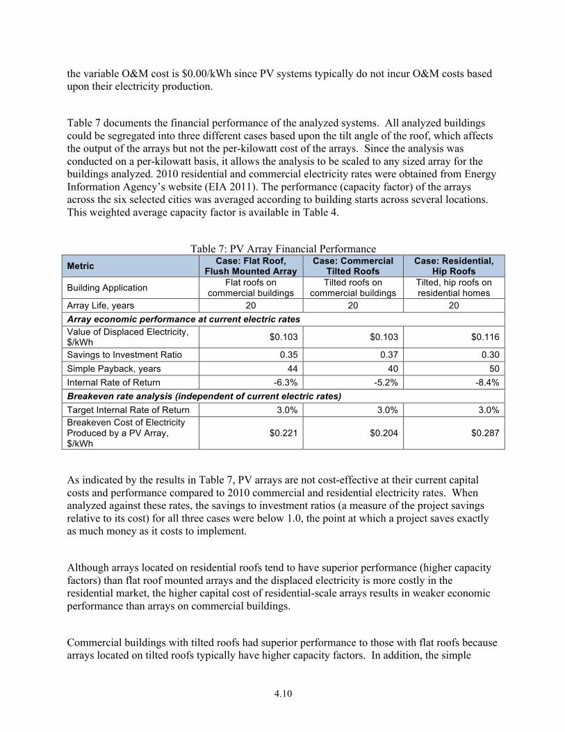
Table 7 documents the financial performance of the analyzed systems. All analyzed buildings could be segregated into three different cases based upon the tilt angle of the roof, which affects the output of the arrays but not the per-kilowatt cost of the arrays. Since the analysis was conducted on a per-kilowatt basis, it allows the analysis to be scaled to any sized array for the buildings analyzed. 2010 residential and commercial electricity rates were obtained from Energy Information Agency’s website (EIA 2011). The performance (capacity factor) of the arrays across the six selected cities was averaged according to building starts across several locations. This weighted average capacity factor is available in Table 4.

Table 7: PV Array Financial Performance Metric Case: Flat Roof,

Flush Mounted Array Case: Commercial

Tilted Roofs Case: Residential,

Hip Roofs

Building Application Flat roofs on commercial buildings

Tilted roofs on commercial buildings

Tilted, hip roofs on residential homes

Array Life, years 20 20 20 Array economic performance at current electric rates Value of Displaced Electricity, $/kWh $0.103 $0.103 $0.116

Savings to Investment Ratio 0.35 0.37 0.30 Simple Payback, years 44 40 50 Internal Rate of Return -6.3% -5.2% -8.4% Breakeven rate analysis (independent of current electric rates) Target Internal Rate of Return 3.0% 3.0% 3.0% Breakeven Cost of Electricity Produced by a PV Array, $/kWh

$0.221 $0.204 $0.287

As indicated by the results in Table 7, PV arrays are not cost-effective at their current capital costs and performance compared to 2010 commercial and residential electricity rates. When analyzed against these rates, the savings to investment ratios (a measure of the project savings relative to its cost) for all three cases were below 1.0, the point at which a project saves exactly as much money as it costs to implement.

Although arrays located on residential roofs tend to have superior performance (higher capacity factors) than flat roof mounted arrays and the displaced electricity is more costly in the residential market, the higher capital cost of residential-scale arrays results in weaker economic performance than arrays on commercial buildings.

Commercial buildings with tilted roofs had superior performance to those with flat roofs because arrays located on tilted roofs typically have higher capacity factors. In addition, the simple

4.11

paybacks are 40 and 50 years for tilted commercial roofs and residential roofs, respectively. This range is well in excess of typical array lifetimes. In addition, the internal rate of return (IRR) for all cases was negative, which indicates that the projects are not cost-effective.

Independent of the 2010 electric rates, a breakeven rate analysis was performed to determine the value of the produced electricity. This electric rate can then be compared to retail electric rates to help gauge if the array is cost-effective. A cost-effective PV array project was defined as having an IRR of at least 3.0%.5 At a 3.0% IRR, the analyzed arrays produced electricity ranging between $0.204/kWh to $0.287/kWh with residential homes producing the most expensive energy and commercial buildings with tilted roofs producing the least costly electricity. Again, arrays located on tilted commercial roofs outperformed those on flat roofs due to the higher capacity factor. At the calculated range, PV arrays cannot compete with grid electricity and will not likely do so for a number of years. However, as more states adopt new renewable portfolio standards (RPSs) requiring renewable energy and specifically solar energy, refine existing RPSs to be more stringent, and as PV module prices decrease and utility electricity prices increase, PV arrays will become more cost-effective and may become an economic option to consider when establishing building energy codes. In some cases, they already are.

PV arrays are currently being developed across the nation. Generally, these arrays are developed under a narrow set of circumstances. First, small- and medium-scale arrays are typically constructed to serve remote, off-grid areas where arrays are a more cost-effective option than new distribution lines. Second, PV arrays are constructed in states with RPSs, and in particular, states with RPSs that:

• Require a certain level of solar energy system development, which is often called a “carve-out” (e.g., Pennsylvania’s RPS requires 0.5% of electricity sold to be sourced from a PV array),

• Require a certain fraction of distributed generation development, a condition that most PV arrays satisfy (e.g., Colorado requires 3.0% of electricity sold to be from distributed systems),

• Require that some or all of the electricity generation is sited in-state or from the local region,

• Limit certain forms of renewable energy development (e.g., Texas has established a goal for non-wind renewable systems),

• Provide a multiplier for solar systems (e.g., Oregon allows energy sourced from a PV array to count as double credit towards meeting RPS mandates),

5 A 0.0% IRR target was not used since most arrays development will require some financing and loan arraignments and since bank account and other low risk deposit options offer interests rates greater than 0.0%. 3.0% was assumed to be a standard interest rate, and therefore reasonable IRR target.

4.12

• Establish suitable non-compliance/alternative compliance fees or fines for not meeting RPS mandates (e.g., a $0.30 charge for every kWh of renewable electricity a utility fails to procure), or

• Combinations of the above listed approaches (e.g., Nevada has both a solar requirement and multipliers for PV systems).

Since states with RPSs require a certain level of renewable energy development, that development may occur at an economic loss in order to meet compliance mandates. Nevertheless, renewable energy developers will naturally seek the most cost-effective renewable energy solution even when all options have suboptimal returns on investment.

If the state RPS does not establish a suitably high non- or alternative-compliance penalty for utilities that do not meet the renewable energy mandate(s), utilities may opt to pay the fee or fine instead of meeting the mandates. For instance, the New Jersey RPS penalty for not meeting the RPS’s solar energy carve-out is $0.658/kWh in 2012, a penalty that is generally more costly than procuring solar electricity. Because of this and the strict limits regarding the siting of eligible solar power plants, solar development in New Jersey is highly active. However, Illinois, a state that also has a solar carve-out, allows up to 50% of a utility’s renewable energy requirement to be satisfied via an alternative compliance payment that requires utilities to pay between $0.00021 and $.000764 for each kilowatt-hour of electricity6 not sourced from an eligible renewable energy system. Since Illinois’s RPS does not vary the alternative compliance payment by source (i.e., the per kilowatt-hour penalty for not satisfying the solar carve-out and the general renewable energy mandate is identical), utilities tend to use the payment to avoid satisfying the more expensive solar carve-out. Illinois utilities are allowed to meet their solar and general renewable energy requirements from renewable energy systems sited over a wide area of the central and eastern United States. Consequently, Illinois does not have an active solar development industry.

Another core aspect of RPSs is that the requirements are dominantly utility requirements to develop and/or procure renewable energy and are not strictly connected to the construction of commercial or residential buildings. To allow non-utility owners of PV arrays or other renewable systems to leverage the RPS requirements to improve renewable energy system economics, system owners must be able to sell their renewable electricity to the utility. Another option is to sell the renewable “attributes” of that electricity without transmitting the electricity itself to the utility. The renewable attribute of a unit of renewable electricity is frequently called a renewable energy credit (REC), and it is typically sold in kilowatt-hour or megawatt-hour blocks. The relationship of RECs to possible energy code requirements are outlined in Dillon et al (Dillon 2011).

Most state RPSs specify that utilities must procure RECs from REC vendors or utility-owned renewable power systems to satisfy an RPS (as opposed to directly purchasing and reselling renewable electricity). This ability to sell RECs to utilities can enable commercial and 6 The range reflects different alternative compliance penalties for different utility service areas.

4.13

residential renewable energy systems to leverage an additional revenue stream in certain circumstances. For instance, in Maryland, another state with an RPS with a solar carve-out, residential and commercial buildings with PV arrays can sell solar RECs (the specific type of REC needed to meet the solar carve-out) for approximately $0.30/kWh in 2011. This revenue stream can then help PV arrays become cost-effective. Then building owners can purchase low-cost RECs available on the national market to replace the solar REC and thus satisfy a building code renewable energy requirement.7 This arrangement is called a REC swap because specialty, non-commodity RECs can be sold to specific customers with specific requirements (i.e., a utility regulated by an RPS), and low-cost commodity RECs can be purchased to replace the high value RECs.

Table 7 provides the REC prices required to result to break even in PV array development. Under the assumptions stated in Tables 6 and 7, solar RECs would need to annually sell for between $0.101 and $0.171 per kilowatt-hour for the array project to have a 3% IRR. This price range is relatively high when compared to wholesale RECs. However, in certain states and markets, solar RECs may be valued at or in excess of this range. Dillon et al. contains a more detailed summary of current REC prices (Dillon 2011)

Ultimately, although REC sales can be used to improve PV and renewable energy system economics, these transactions are highly localized to specific states with specific RPS conditions. Consequently, these opportunities are challenging to incorporate into a high-level, national analysis. Furthermore, the introduction of renewable energy system requirements into building codes may have unforeseen effects on local and state REC markets. These effects should be considered when performing more rigorous assessments.

7 Note, this option may not be completely available to the utility because the RPS language may establish geographic restrictions on REC or solar REC procurement. However, building owners are not bound by the same limits.

5.14

5.0 Conclusions and Recommendations

This analysis work has presented energy and economic analysis for future energy code requirements of renewable energy generation. Several important conclusions are possible based on this analysis work:

• It is reasonable to consider a higher on-site renewable generation requirement for commercial buildings than that proposed by Kaufman et al. The present analysis indicates 6 watts/sf as a nationwide average, with possible exceptions for specific building types.

• The on-site renewable generation requirement for residential buildings should be 4 watts/sf.

• PV is not currently economic compared to the average commercial or residential electricity rates. However, site-specific requirements and the ability to trade RECs may result in economic systems in some locations. Future requirements and incentives may result in more favorable economic conditions in the future.

The PV array analysis by location and building type shows the most variation in install density by building type. PV performance and therefore economics varies by location and roof type. It may be important to structure the code requirement based on building type. A more detailed analysis with additional locations might confirm if a national average requirement level is appropriate or if specific climate zones should have lower prescriptive levels. The economic analysis has been done at a national average level. A more meaningful analysis might be performed for each of the cities or climate zones of interest with region-specific electricity rate information.    

6.15

 6.0 References

California Solar Initiative (CSI). Accessed June 2011 at http://www.gosolarcalifornia.org/csi/index.php. Dillon, H.E., Antonopoulos, C.A., Solana, A.E., Russo, B.J. 2011. Renewable Energy Requirements for Future Building Codes: Options for Compliance. Pacific Northwest National Laboratory, Richland WA: PNNL-20727. Energy Information Agency (EIA), Department of Energy. Accessed August 2011. http://www.eia.gov/cneaf/electricity/epm/table5_3.html Kaufman, J.R., Hand, J.R., Halverson, M. 2011. Integrating Renewable Energy Requirements Into Building Energy Codes. Pacific Northwest National Laboratory, Richland WA: PNNL-20442. NREL. 2011. Insolation for Flat-Plate Collectors at Latitude Tilt Map. Accessed August 22, 2011 at http://www.nrel.gov/gis/images/map_pv_national_hi-­‐res.jpg    National Institute of Standards and Technology (NIST). Energy Price Indices and Discount Factors for Life-Cycle Cost Analysis. May 2010. Accessed August 2011 at http://www1.eere.energy.gov/femp/pdfs/ashb10.pdf. Taylor, Z.T., Lucas, R. 2010. An Estimate of Residential Energy Savings From IECC Change Proposals Recommended for Approval at the ICC’s Fall, 2009, Initial Action Hearings. Pacific Northwest National Laboratory, Richland WA: PNNL-19367. U.S. Department of Energy (DOE). Energy Efficiency and Renewable Energy. 2011. Request for Information on Cost Effective Residential Energy Codes. Accessed July 20, 2011 at http://www.gpo.gov/fdsys/pkg/FR-2011-09-13/pdf/2011-23236.pdf

6.16

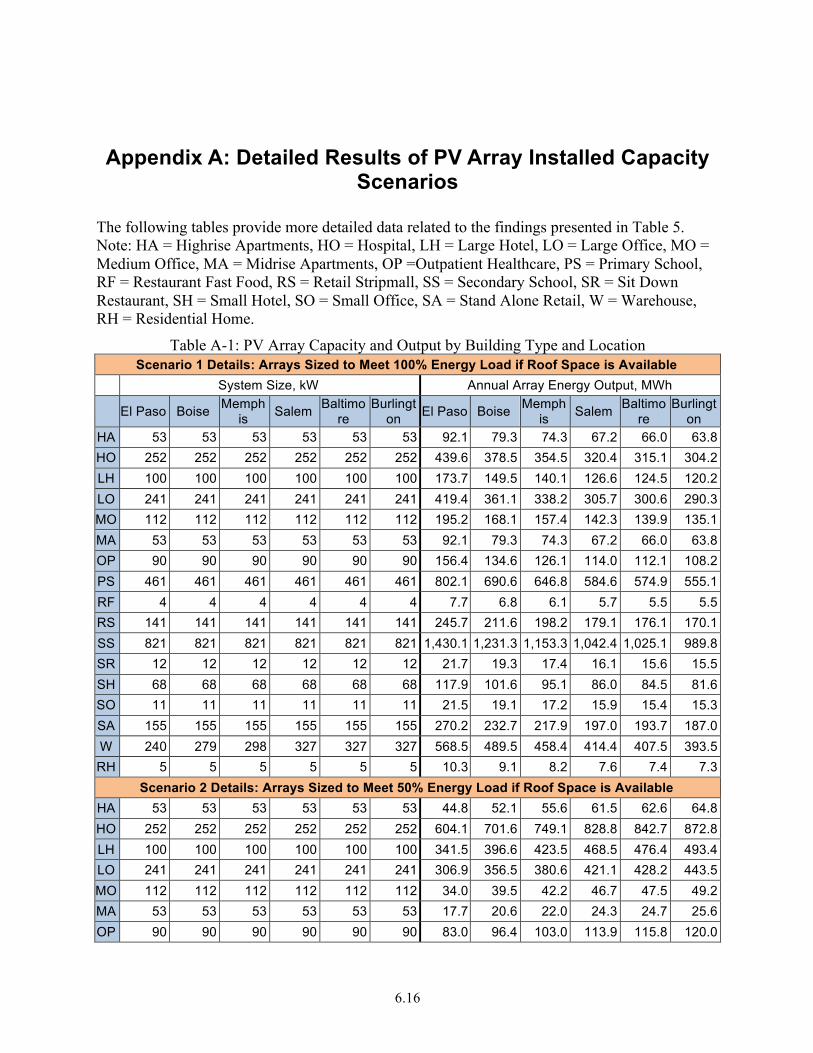
Appendix A: Detailed Results of PV Array Installed Capacity Scenarios

The following tables provide more detailed data related to the findings presented in Table 5. Note: HA = Highrise Apartments, HO = Hospital, LH = Large Hotel, LO = Large Office, MO = Medium Office, MA = Midrise Apartments, OP =Outpatient Healthcare, PS = Primary School, RF = Restaurant Fast Food, RS = Retail Stripmall, SS = Secondary School, SR = Sit Down Restaurant, SH = Small Hotel, SO = Small Office, SA = Stand Alone Retail, W = Warehouse, RH = Residential Home.

Table A-1: PV Array Capacity and Output by Building Type and Location Scenario 1 Details: Arrays Sized to Meet 100% Energy Load if Roof Space is Available

System Size, kW Annual Array Energy Output, MWh

El Paso Boise Memphis Salem Baltimo

re Burlingt

on El Paso Boise Memphis Salem Baltimo

re Burlingt

on HA 53 53 53 53 53 53 92.1 79.3 74.3 67.2 66.0 63.8 HO 252 252 252 252 252 252 439.6 378.5 354.5 320.4 315.1 304.2 LH 100 100 100 100 100 100 173.7 149.5 140.1 126.6 124.5 120.2 LO 241 241 241 241 241 241 419.4 361.1 338.2 305.7 300.6 290.3 MO 112 112 112 112 112 112 195.2 168.1 157.4 142.3 139.9 135.1 MA 53 53 53 53 53 53 92.1 79.3 74.3 67.2 66.0 63.8 OP 90 90 90 90 90 90 156.4 134.6 126.1 114.0 112.1 108.2 PS 461 461 461 461 461 461 802.1 690.6 646.8 584.6 574.9 555.1 RF 4 4 4 4 4 4 7.7 6.8 6.1 5.7 5.5 5.5 RS 141 141 141 141 141 141 245.7 211.6 198.2 179.1 176.1 170.1 SS 821 821 821 821 821 821 1,430.1 1,231.3 1,153.3 1,042.4 1,025.1 989.8 SR 12 12 12 12 12 12 21.7 19.3 17.4 16.1 15.6 15.5 SH 68 68 68 68 68 68 117.9 101.6 95.1 86.0 84.5 81.6 SO 11 11 11 11 11 11 21.5 19.1 17.2 15.9 15.4 15.3 SA 155 155 155 155 155 155 270.2 232.7 217.9 197.0 193.7 187.0 W 240 279 298 327 327 327 568.5 489.5 458.4 414.4 407.5 393.5 RH 5 5 5 5 5 5 10.3 9.1 8.2 7.6 7.4 7.3

Scenario 2 Details: Arrays Sized to Meet 50% Energy Load if Roof Space is Available HA 53 53 53 53 53 53 44.8 52.1 55.6 61.5 62.6 64.8 HO 252 252 252 252 252 252 604.1 701.6 749.1 828.8 842.7 872.8 LH 100 100 100 100 100 100 341.5 396.6 423.5 468.5 476.4 493.4 LO 241 241 241 241 241 241 306.9 356.5 380.6 421.1 428.2 443.5 MO 112 112 112 112 112 112 34.0 39.5 42.2 46.7 47.5 49.2 MA 53 53 53 53 53 53 17.7 20.6 22.0 24.3 24.7 25.6 OP 90 90 90 90 90 90 83.0 96.4 103.0 113.9 115.8 120.0

6.17

PS 434 461 461 461 461 461 69.2 80.4 85.9 95.0 96.6 100.0 RF 4 4 4 4 4 4 17.3 19.5 21.6 23.3 24.2 24.3 RS 141 141 141 141 141 141 22.8 26.4 28.2 31.2 31.7 32.9 SS 821 821 821 821 821 821 199.1 231.3 246.9 273.2 277.8 287.7 SR 12 12 12 12 12 12 26.5 29.9 33.2 35.8 37.1 37.3 SH 68 68 68 68 68 68 40.1 46.6 49.7 55.0 55.9 57.9 SO 11 11 11 11 11 11 2.7 3.1 3.4 3.7 3.8 3.8 SA 148 155 155 155 155 155 23.6 27.4 29.2 32.4 32.9 34.1 W 120 139 149 165 167 173 19.1 22.2 23.7 26.3 26.7 27.6 RH 5 5 5 5 5 5 9.9 8.2 7.4 7.6 9.1 7.3

Scenario 2 Details: Arrays Sized to Meet 10% Energy Load if Roof Space is Available HA 53 53 53 53 53 53 9.0 10.4 11.1 12.3 12.5 13.0 HO 252 252 252 252 252 252 120.8 140.3 149.8 165.8 168.5 174.6 LH 100 100 100 100 100 100 68.3 79.3 84.7 93.7 95.3 98.7 LO 241 241 241 241 241 241 61.4 71.3 76.1 84.2 85.6 88.7 MO 43 50 53 59 60 62 6.8 7.9 8.4 9.3 9.5 9.8 MA 22 26 28 31 31 32 3.5 4.1 4.4 4.9 4.9 5.1 OP 90 90 90 90 90 90 16.6 19.3 20.6 22.8 23.2 24.0 PS 87 101 108 119 121 126 13.8 16.1 17.2 19.0 19.3 20.0 RF 4 4 4 4 4 4 3.5 3.9 4.3 4.7 4.8 4.9 RS 29 33 35 39 40 41 4.6 5.3 5.6 6.2 6.3 6.6 SS 250 290 310 343 349 361 39.8 46.3 49.4 54.6 55.6 57.5 SR 12 12 12 12 12 12 5.3 6.0 6.6 7.2 7.4 7.5 SH 50 58 62 68 68 68 8.0 9.3 9.9 11.0 11.2 11.6 SO 3 4 4 5 5 5 0.5 0.6 0.7 0.7 0.8 0.8 SA 30 34 37 41 41 43 4.7 5.5 5.8 6.5 6.6 6.8 W 24 28 30 33 33 35 3.8 4.4 4.7 5.3 5.3 5.5 RH 1 2 1 2 2 3 2.0 2.0 2.9 2.4 2.9 4.6

6.18

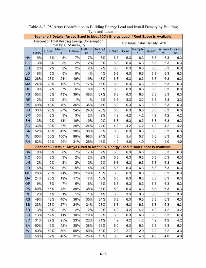
Table A-2: PV Array Contribution to Building Energy Load and Install Density by Building Type and Location

Scenario 1 Details: Arrays Sized to Meet 100% Energy Load if Roof Space is Available

Percent of Total Building Energy Consumption

met by a PV Array, % PV Array Install Density, W/sf

El

Paso Boise Memphis Salem Baltimo

re Burlingt

on El Paso Boise Memphis Salem Baltimo

re Burlingt

on HA 9% 8% 8% 7% 7% 7% 6.3 6.3 6.3 6.3 6.3 6.3 HO 3% 3% 3% 2% 2% 2% 6.3 6.3 6.3 6.3 6.3 6.3 LH 2% 2% 2% 2% 2% 2% 6.3 6.3 6.3 6.3 6.3 6.3 LO 6% 5% 5% 5% 4% 4% 6.3 6.3 6.3 6.3 6.3 6.3 MO 26% 23% 21% 19% 19% 18% 6.3 6.3 6.3 6.3 6.3 6.3 MA 24% 20% 19% 17% 17% 16% 6.3 6.3 6.3 6.3 6.3 6.3 OP 9% 7% 7% 6% 6% 6% 6.3 6.3 6.3 6.3 6.3 6.3 PS 53% 46% 43% 39% 38% 37% 6.3 6.3 6.3 6.3 6.3 6.3 RF 2% 2% 2% 1% 1% 1% 3.3 3.3 3.3 3.3 3.3 3.3 RS 49% 43% 40% 36% 35% 34% 6.3 6.3 6.3 6.3 6.3 6.3 SS 33% 28% 27% 24% 24% 23% 6.3 6.3 6.3 6.3 6.3 6.3 SR 3% 3% 3% 3% 2% 2% 4.2 4.2 4.2 4.2 4.2 4.2 SH 13% 12% 11% 10% 10% 9% 6.3 6.3 6.3 6.3 6.3 6.3 SO 33% 30% 27% 25% 24% 24% 4.2 4.2 4.2 4.2 4.2 4.2 SA 52% 45% 42% 38% 38% 36% 6.3 6.3 6.3 6.3 6.3 6.3 W 100% 100% 100% 99% 98% 94% 4.6 5.4 5.7 6.3 6.3 6.3 RH 52% 32% 40% 31% 26% 16% 4.0 4.0 4.0 4.0 4.0 4.0

Scenario 2 Details: Arrays Sized to Meet 50% Energy Load if Roof Space is Available HA 9% 8% 8% 7% 7% 7% 6.3 6.3 6.3 6.3 6.3 6.3 HO 3% 3% 3% 2% 2% 2% 6.3 6.3 6.3 6.3 6.3 6.3 LH 2% 2% 2% 2% 2% 2% 6.3 6.3 6.3 6.3 6.3 6.3 LO 6% 5% 5% 5% 4% 4% 6.3 6.3 6.3 6.3 6.3 6.3 MO 26% 23% 21% 19% 19% 18% 6.3 6.3 6.3 6.3 6.3 6.3 MA 24% 20% 19% 17% 17% 16% 6.3 6.3 6.3 6.3 6.3 6.3 OP 9% 7% 7% 6% 6% 6% 6.3 6.3 6.3 6.3 6.3 6.3 PS 50% 46% 43% 39% 38% 37% 5.9 6.3 6.3 6.3 6.3 6.3 RF 2% 1% 1% 1% 1% 1% 3.3 3.3 3.3 3.3 3.3 3.3 RS 49% 43% 40% 36% 35% 34% 6.3 6.3 6.3 6.3 6.3 6.3 SS 33% 28% 27% 24% 24% 23% 6.3 6.3 6.3 6.3 6.3 6.3 SR 3% 3% 3% 2% 2% 2% 4.2 4.2 4.2 4.2 4.2 4.2 SH 13% 12% 11% 10% 10% 9% 6.3 6.3 6.3 6.3 6.3 6.3 SO 31% 27% 25% 23% 22% 21% 4.2 4.2 4.2 4.2 4.2 4.2 SA 50% 45% 42% 38% 38% 36% 6.0 6.3 6.3 6.3 6.3 6.3 W 50% 50% 50% 50% 50% 50% 2.3 2.7 2.9 3.2 3.2 3.3 RH 50% 32% 40% 31% 26% 16% 3.8 4.0 4.0 4.0 4.0 4.0

6.19

Scenario 2 Details: Arrays Sized to Meet 10% Energy Load if Roof Space is Available HA 9% 8% 8% 7% 7% 7% 6.3 6.3 6.3 6.3 6.3 6.3 HO 3% 3% 3% 2% 2% 2% 6.3 6.3 6.3 6.3 6.3 6.3 LH 2% 2% 2% 2% 2% 2% 6.3 6.3 6.3 6.3 6.3 6.3 LO 6% 5% 5% 5% 4% 4% 6.3 6.3 6.3 6.3 6.3 6.3 MO 10% 10% 10% 10% 10% 10% 2.4 2.8 3.0 3.3 3.3 3.4 MA 10% 10% 10% 10% 10% 10% 2.6 3.1 3.3 3.6 3.7 3.8 OP 9% 7% 7% 6% 6% 6% 6.3 6.3 6.3 6.3 6.3 6.3 PS 10% 10% 10% 10% 10% 10% 1.2 1.4 1.5 1.6 1.7 1.7 RF 2% 1% 1% 1% 1% 1% 3.3 3.3 3.3 3.3 3.3 3.3 RS 10% 10% 10% 10% 10% 10% 1.3 1.5 1.6 1.7 1.8 1.8 SS 10% 10% 10% 10% 10% 10% 1.9 2.2 2.4 2.6 2.7 2.8 SR 3% 3% 3% 2% 2% 2% 4.2 4.2 4.2 4.2 4.2 4.2 SH 10% 10% 10% 10% 10% 9% 4.7 5.4 5.8 6.3 6.3 6.3 SO 9% 9% 9% 9% 9% 9% 1.2 1.4 1.6 1.7 1.7 1.7 SA 10% 10% 10% 10% 10% 10% 1.2 1.4 1.5 1.6 1.7 1.7 W 10% 10% 10% 10% 10% 10% 0.5 0.5 0.6 0.6 0.6 0.7 RH 10% 10% 10% 10% 10% 10% 0.8 1.2 1.0 1.3 1.5 2.5