Rendering of 3D Scalar and Vector Fields at LLNL

Roger Crawfis, Nelson Max, Barry Becker, Brian Cabral

Lawrence Livermore National LaboratoryP.O. Box 808

Livermore, CA 94551

Abstract

Simulation of complex 3-dimensional phenomena generateaizta sets which are hard to comprehend using conventional2-dimensionally oriented visualization tools. One way toovercome this limitation is to employ various volumevisualization techniques. While early volume visualizationtechniques worked well on simple scalar volumes theyfailed to exploit frame bufler hardware capabilities andhandle higher order data such as vector jields, Work atLawrence Livermore National Laboratory has centered ondeveloping new techniques and extending existingtechniques. This paper describes the various algorithmsdeveloped for volume rendering, and presents new melhodsof examining vector fields in a volumetric fashion.

Introduction

Computer simulations dealing with theatmosphere, the ocean, hydrodynamics, electro-magnetic, structural response, andenvironmental clean up, generate very large andcomplex data sets consisting of not only severalscalar variables, but also vector and tensorquantities. Understanding an individual scalarfield from a three-dimensional simulation is oftendifficult with current visualization tools.Understanding 3D vector fields and complexrelationships is even more arduous. In order tounderstand the tens of gigabytes of data beinggenerated from today’s supercomputers, bettervisualization techniques and tools are needed.Better visualization tools are even more urgent aswe progress to massively parallel architecturesand larger more complex problems.

Volume rendering allows us to examine asubstantial amount of a single 3D scalar field at asingle time step. Research into visualizing 3Dscalar fields has progressed over the past fewyears from iso-contour surfaces, to direct volumerendering of regularly gridded data, and thenirregularly structured data, but all methodsoperate on a single scalar field. A minor amountof effort ‘has been placed on understanding theinteractions between several scalar fields. Even

@ 1993 ACM 0-8186-4340-4/930011 $1.50

less effortunderstanding

has been directed towardsvector or tensor fields. Correcting

these deficiencies has been the thrust of OU;research. This paper describes the variousalgorithms developed for volume rendering, andpresents new methods of examining vector fieldsin a volumetric fashion.

Volume Rendering

The rendering of three-dimensional scalar fieldshas received much attention over the past severalyears. There are three common ways to visualizea scalar function in a volume (1) interactivelymove a color coded 2D slice through the volume[Nielson90], (2) draw contour surfaces[Lorensen87], or (3) integrate a continuos volumedensity along viewing rays [Max90]. The secondmethod is a generalization of plotting contourlines in 2D. The other methods generalize thecolor coding of a 2D scalar field, although the 3Dcolor field can only be viewed in either 2D slicesor projections. The first two methods aregenerally termed indirect volume rendering, whilethe third method is termed direct v 01 u merendering, or simply volume rendering. Theseterms imply the basic architecture of thetechniques: indirect volume rendering convertsthe 3D field into geometric surface primitiveswhich are then rendered to form an image, whiledirect volume rendering converts the field directlyinto the image. Henceforth, we will use the termvolume rendering to refer strictly to direct volumerendering.

There has been much research on volumerendering algorithms over the past few years,leading to several competing algorithms. Fourcommon approaches to volume rendering are (1)ray tracing, (2) analytical scan conversion, (3)hardware compositing, and (4) splatting. Variousadvantages/disadvantages exist with each of these

algorithms. Many flavors of each of thesealgorithms also exist. We have implemented aversion of each of these and extended them to

Pertiswn to copy without fee all or pal of Ibis material is granted,

provided that the copies are not made or distributed for dirw+ commercialadvantage, the ACM copyright ndice and the title of the publication and

570h date appear, and notice is given that copying is by pxmission cf tbeAwxiation for Computing Machinev. To copy dher.vi=, m 10republish,requires a fee andkx specific permission.

examine vector fields rather than or in addition toa single scalar field.

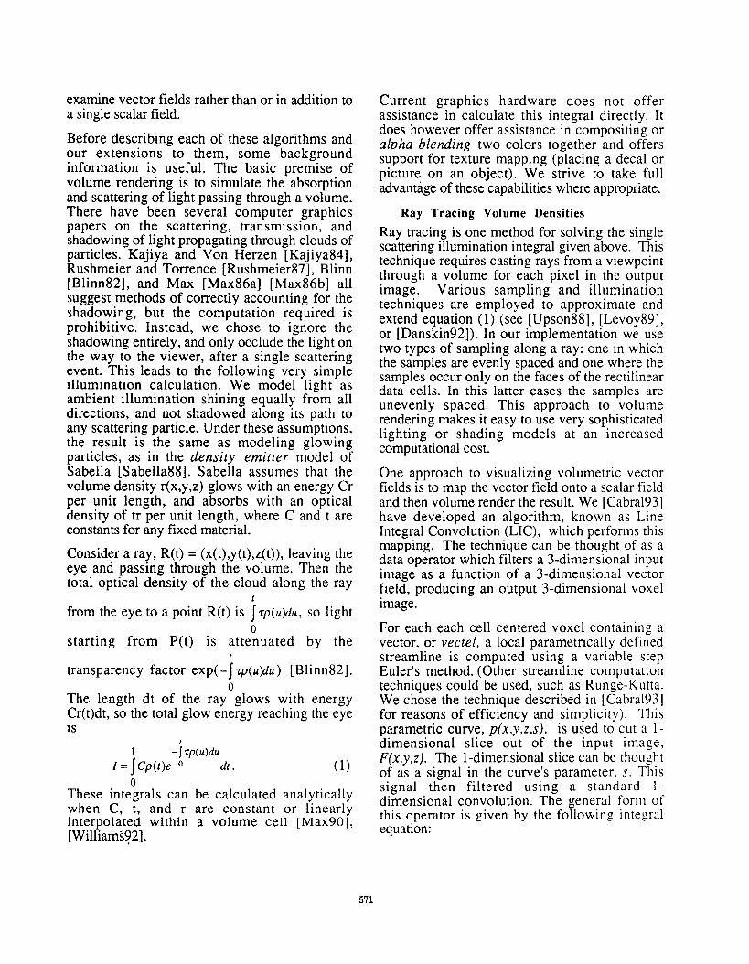
Before describing each of these algorithms andour extensions to them, some backgroundinformation is useful. The basic premise ofvolume rendering is to simulate the absorptionand scattering of light passing through a volume.There have been several computer graphicspapers on the scattering, transmission, andshadowing of light propagating through clouds ofparticles. Kajiya and Von Herzen [Kajiya84],Rushmeier and Torrence [Rushmeier87], Blinn[Blinn82], and Max [Max86a] [Max86b] allsuggest methods of correctly accounting for theshadowing, but the computation required isprohibitive. Instead, we chose to ignore theshadowing entirely, and only occlude the light onthe way to the viewer, after a single scatteringevent. This leads to the following very simpleillumination calculation. We model light asambient illumination shining equally from alldirections, and not shadowed along its path toany scattering particle. Under these assumptions,the result is the same as modeling glowingparticles, as in the density emitter model ofSabella [Sabella88]. Sabella assumes that thevolume density r(x,y,z) glows with an energy Crper unit length, and absorbs with an opticaldensity of tr per unit length, where C and t areconstants for any fixed material.

Consider a ray, R(t) = (x(t),y(t),z(t)), leaving theeye and passing through the volume. Then thetotal optical density of the cloud along the ray

from the eye to a point R(t) is ~zp(u)du, so light

starting from P(t) is atte~uated by the

transparency factor exp( -~ zp(u)du ) [Blinn82].o

The length dt of the ray glows with energyCr(t)dt, so the total glow energy reaching the eyeis

1 +p(u)du

I = ~Cp(f)e 0 dt . (1)

These inte&als can be calculated analyticallywhen C, t, and r are constant or linearlyinterpolated within a volume cell [Ivlax90],

[Williams92].

Current graphics hardware does not offerassistance in calculate this integral directly. Itdoes however offer assistance in compositing oralpha-blending two colors together and offerssupport for texture mapping (placing a decal orpicture on an object). We strive to take fulladvantage of these capabilities where appropriate.

Ray Tracing Volume Densities

Ray tracing is one method for solving the single

scattering illumination integral given above. Thistechnique requires casting rays from a viewpointthrough a volume for each pixel in the outputimage, Various sampling and illuminationtechniques are employed to approximate andextend equation (1) (see [Upson88], [Levoy89],or [Danskin92] ). In our implementation we usetwo types of sampling along a ray: one in whichthe samples are evenly spaced and one where thesamples occur only on the faces of the rectilineardata cells. In this latter cases the samples areunevenly spaced. This approach to volumerendering makes it easy to use very sophisticatedlighting or shading models at an increasedcomputational cost.

One approach to visualizing volumetric vectorfields is to map the vector field onto a scalar fieldand then volume render the result. We [Cabra193]have developed an algorithm, known as LineIntegral Convolution (LIC), which performs thismapping. The technique can be thought of as adata operator which filters a 3-dimensional inputimage as a function of a 3-dimensional vectorfield, producing an output 3-dimensional voxelimage.

For each each cell centered voxel containing avector, or vectel, a local parametrically definedstreamline is computed using a variable stepEuler’s method. (Other streamline computationtechniques could be used, such as Runge-Kutta.We chose the technique described in [Cabra193]for reasons of efficiency and simplicity). Thisparametric curve, p(x,y,z,s), is used to cut a 1-dimensional slice out of the input image,F(x,y,z). The l-dimensional slice can be thoughtof as a signal in the curve’s parameter, .s. Thissignal then filtered using a standard 1-dimensional convolution. The general form ofthis operator is given by the following integralequation:

571

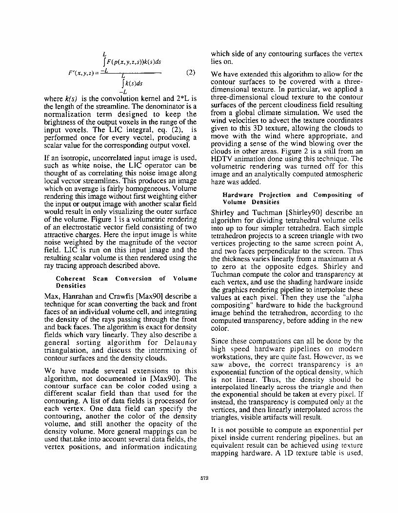
L

p(P(x,Y,z,s))wfs

F’(x,y,z) = -L ~ (2)

~k(s)ds

-Lwhere k(s) is the convolution kernel and 2*L isthe length of the streamline. The denominator is anormalization term designed to keep thebrightness of the output voxels in the range of theinput voxels. The LIC integral, eq. (2), isperformed once for every vectel, producing ascalar value for the corresponding output voxel.

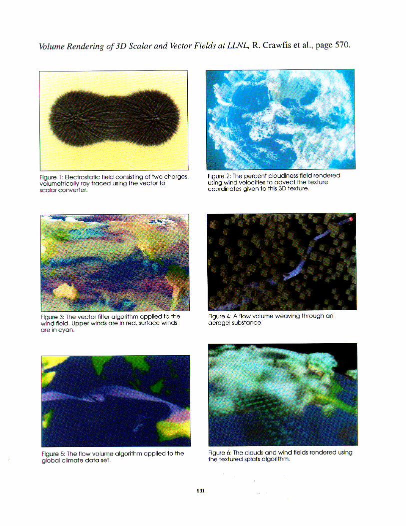
If an isotropic, uncorrelated input image is used,such as white noise, the LIC operator can bethought of as correlating this noise image alonglocal vector streamlines. This produces an imagewhich on average is fairly homogeneous. Volumerendering this image without first weighting eitherthe input or output image with another scalar fieldwould result in only visualizing the outer surfaceof the volume. Figure 1 is a volumetric renderingof an electrostatic vector field consisting of twoattractive charges. Here the input image is whitenoise weighted by the magnitude of the vectorfield. LIC is run on this input image and theresulting scalar volume is then rendered using theray tracing approach described above.

Coherent Scan Conversion of VolumeDensities

Max, Hanrahan and Crawfis [Max90] describe atechnique for scan converting the back and frontfaces of an individual volume cell, and integratingthe density of the rays passing through the frontand back faces. The algorithm ‘is exact for densityfields which vary linearly. They also describe ageneral sorting algorithm for Delaunaytriangulation, and discuss the intermixing ofcontour surfaces and the density clouds.

We have made several extensions to thisalgorithm, not documented in [Max90]. Thecontour surface can be color coded using a

different scalar field than that used for thecontouring. A list of data fields is processed foreach vertex. One data field can specify thecontouring, another the color of the densityvolume, and still another the opacity of thedensity volume. More general mappings can beused that.mke into account several data fields, thevertex positions, and information indicating

which side of any contouring surfaces the vertexlies on.

We have extended this algorithm to allow for thecontour surfaces to be covered with a three-dimensional texture. In particular, we applied athree-dimensional cloud texture to the contoursurfaces of the percent cloudiness field resultingfrom a global climate simulation. We used thewind velocities to advect the texture coordinatesgiven to this 3D texture, allowing the clouds tomove with the wind where appropriate, andproviding a sense of the wind blowing over theclouds in other areas. Figure 2 is a still from anHDTV animation done using this technique. Thevolumetric rendering was turned off for thisimage and an analytically computed atmospherichaze was added.

Hardware Projection and Compositing ofVolume Densities

Shirley and Tuchman [Shirley90] describe analgorithm for dividing tetrahedral volume cellsinto up to four simpler tetrahedral. Each simpletetrahedron projects to a screen triangle with twovertices projecting to the same screen point A,and two faces perpendicular to the screen. Thusthe thickness varies linearly from a maximum at Ato zero at the opposite edges. Shirley andTuchman compute the color and transparency ateach vertex, and use the shading hardware insidethe graphics rendering pipeline to interpolate thesevalues at each pixel. Then they use the “alphacompositing” hardware to hide the backgroundimage behind the tetrahedron, according to thecomputed transparency, before adding in the newcolor.

Since these computations can all be done by thehigh speed hardware pipelines on modernworkstations, they are quite fast. However, as wesaw above, the correct transparency is anexponential function of the optical density, whichis not linear. Thus, the density should beinterpolated linearly across the mangle and then

the exponential should be taken at every pixel. Ifinstead, the transparency is computed only at thevertices, and then linearly interpolated across thetriangles, visible artifacts will result.

It is not possible to compute an exponential perpixel inside current rendering pipelines, but anequivalent result can be achieved using texturemapping hardware. A ID texture table is used,

572

which is addressed by the optical density, andreturns the transparency. The texture coordinate isthen specified as the optical density at eachvertex, and will be interpolated across the mangleby the shading hardware, before being used as atexture address. This gives an accuratetransparency for every pixel, and eliminates theartifacts.

We use this algorithm for a new vectorvisualization technique which we call flowvolumes [Max93b]. We have extended theconcept of stream lines or flow ribbons to theirvolume equivalent. A seed polygon is placed intothe flow field under user control. This polygonacts as a smoke generator. As the vector fieldpasses through the polygon, smoke is propagatedforward, sweeping out a volume (Figure 5)which is subdivided into tetrahedral, Compressionand expansion of the volume due to the ilow canbe taken into account by adjusting the opacitybased on the tetrahedron’s volume. As the flowvolume expands, we employ an adaptive meshrefinement technique to ensure the curvature ofthe resulting volume is accurate. The complextopology of the flow volume would require ageneral sorting method to yield a valid back-to-front sort. However, for this application, we canrequire that the smoke or dye be a constant colorthroughout the volume. It can then be shown[Max93b] that the resulting integration of thevolume density is independent of the order thevolume cells are processed. Thus, no sorting isrequired. Since we are only rendering the smoke,and not an entire volume, and using the hardwarefor the rendering, we have achieved real-timeinteraction. We have also added additionalfeatures that allow the user to watch moving puffsof smoke, control the time propagation of thesmoke, and combine opaque geometry with thesmoke. Figure 4 shows an aerogel simulation,where the tiny cubes are the zones containing theaerogel, and the blue smoke represents a flowthrough the aerogel.

Hardware Splatting of Volume Densities

Westover [Westover89] used an idea calledsplatting, where each voxel is treated as a singlesampling point and a continuos 3D signal isreconstructed. The contribution of each voxelpoint to the volume density is then determined byits reconstruction kernel, and these arecomposite into the image independently in back-

to-front order. Westover [Westover90] later usedan accumulation buffer to reconstruct an entiresheet’s contribution before it is composite intothe image. Since the individual splats overlap,this avoids problems in the sorting, however, amuch more noticeable change in the volumedensity occurs when the arrangement into sheetsmust change.

Laur and Hanrahan [Laur91] extended thesplatting technique to handle hierarchicalrepresentations of the sampled data field. Theyalso approximated the gaussian used in thereconstruction by a small polygonal mesh andutilized the graphics hardware to render the splat.This allowed for a quick coarse representation ofthe data that evolved into a more accuraterepresentation adaptively. The Explorer productfrom SGI uses a variant of this technique withoutthe adaptive refinement.

In reconstructing the 3D signal, a gaussianfunction is usually used. An unattractive propertyof this is its infinite extent. Every splattheoretically contributes to the entire volumedensity. Some finite extent is usually chosen andthe splat is either abruptly cut-off or forced tozero. Max [Max92] uses an optimal quadraticfunction with a limited extent for thereconstruction of 2D signals. We [Crawfis93]have extended this for a cubic function for thereconstruction of 3D signals, which is optimal forall viewing angles. Using this function as ahardware texture map on a simple square splatgives a more accurate rendering of the volumedensity, and for large problems consisting ofmany small splats is actually faster than using thepolygonal mesh of [Laur9 1]. We have added thisto the Explorer system.

We [Crawfis92] developed a methodology forintegrating a vector representation into the scalarsplat. This algorithm however uses a samplingand reconstruction approach (which we called afilter) and does not make use of the graphicshardware. Figure 3. illustrates this technique forthe wind field of a global climate simulation. We[Crawfis93] have now merged this concept withvolume rendering via splatting by extending thetexture splats above to include an anisotropicrepresentation of the vector field. The splat is notonly oriented perpendicular to the viewing

direction, but also rotated to align the texture with

the projected vector direction. A table of textures

573

with different vector lengths is used toforeshorten the vector as its direction becomesparallel to the viewing direction. By using theappropriate controls of the texture mappinghardware, the volume density can be representedusing one color scheme, and the vector fieldrepresented using another. Figure 6 shows thepercent cloudiness field and the wind velocitiesfor the global climate simulation. By cyclingthrough a sequence of textures with changingdisplacements, we can make the textures move inthe flow specified by the vector field.

Sorting

The scan conversion, hardware projection, andsplatting methods of volume rendering all requirea back to front sort of the volume cells. Forrectangular lattices, the location of the viewpointwithin the data volume (or of its projection onto aface or edge of the data volume) can easily beused to specify a sorting order. This sortingmethod extends recursively to octree or otherrectilinear adaptive mesh refinements. For a moregeneral mesh of convex data without holes,sorting can be done using a topological sort[Knuth73] [Max90] on a directed graphrepresenting cell adjacency (with the direction ofan edge specifying which of the two adjunct cellsis in front). This sort may detect cycles, but it canbe proved that cycles do not occur for Delaunaytriangulations. [Edelsbrunner89], [Max90], or forthe particular geometries which occur in ourclimate simulations [Max93a]. We are alsoworking on a version of the Newell, Newell, andSancha sort [Newel172] applied to volume cellsinstead of to polygons. This algorithm will splitoffending cells when cycles are detected. It alsodoes not require the adjacency information, whichmay not be available in certain situations (forexample, finite element simulations with slidinginterfaces), and can deal with non convexvolumes with holes. Williams [Williams91 ] alsogeneralizes the directed graph method to non-convex data volumes, but his method is notguaranteed to be correct.

Conclusions

We have explored the use of volume renderingfor scientific visualization and extended thealgorithms for representing vector field data aswell as scalar field data. The algorithms cover awide gamut of techniques, from the veryinteractive flow volume generator for studying

specific areas, to the ray-traced vector volumesand vector splatting techniques for representingglobal views of the vector field. These algorithmsare a necessary step towards better visualizationtechniques for large data sets produced fromcomplex three-dimensional simulations onsupercomputers and massively parallel machines.

This paper has given a broad overview of ourwork. More details can be found in thereferences: [Max90], [Crawfis91 ], [Crawfis92],[Max92], [Cabra193], [Crawfis93], [Max93a],and [Max93b]. These papers also give other newmaterial on the usage of volume rendering andour extensions to vector field rendering.

Future Work

Most of the extensions mentioned here are in theirearly development. Much work is still needed inapplying them to various application data andmaking refinements. In particular, the properchoice of textures for the textured isocontour andthe vector splatting techniques is an open area ofresearch. Better subdivision and splittingalgorithms are needed for the flow volumealgorithm. We have also developed the basicframework for multivariate representations, buthave only tried it out for very simple mappings.More complex mappings (presumably applicationspecific) need to be studied, and a more efficientand flexible framework put into place.

Acknowledgments

The authors are indebted to the many people whoprovided the data used in the visualization in thispaper. Tony Ladd and Elaine Chandler providedthe aerogel data. The climate data is courtesy ofJerry Potter, the Program for Climate ModelDiagnosis and Intercomparison at Livermore, andthe European Centre for Medium-range WeatherForecasts. The authors would like to thank ChuckGrant for many helpful comments. This workwas performed under the auspices of the USDepartment of Energy by Lawrence LivermoreNational Laboratory under contract number W-7405 -ENG-48, with specific support from aninternal (LDRD) research grant.

References

[Blinn82] Blinn, James, Light Reflection Functions for

Simulation of Clouds and Dusty Surfaces.

Computer Graphics Vol. 16 No. 3 (Siggraph ’82)

pp. 21-29.

574

[Cabra193] Cabral, Brian and Casey Leedom, Imaging Vector

Fields Using Line Integral Convolution,

[Crawfis91] Crawfis, Roger and Michael Allison. A ScientificVisualization Synthesizer. In Proceedings

Visualization ’91. Gregory Nielson and Larry

Rosenblum eds., IEEE Los Akunitos, CA, pp.262-267.

[Craw fis92] Crawfis, Roger and Nelson Max, Direct VolumeVisualization of Three-Dimensional Vector

Fields. Proceedings of the 1992 Workshop onVolume Visualization (October 1992), ACMSIGGRAPH New York. pp. 55-60.

[Crawfis93] Crawfis, Roger and Nelson Max, Texture Splats

for 3D Vector and Scalar Field Visualization. In

Proceedings Visualization ’93 (October 1993),IEEE Los Alarnitos, CA, pp. 261-266

[Danskin92] Danskin, John and Pat Hanrahan, Fas rAlgorithms for Volume Ray Tracing. Proceedingsof the 1992 Workshop on Volume Visualization(October 1992), ACM SIGGRAPH New York. pp.

91-98.

[Edelsbrunner89 ]Edelsbrunner, Herbert An Acyclicity

Theorem in Cell Complexes in d Dimensions.Proceedings of the ACM Symposium onComputational Geometry (1989) pp. 145-151.

[Kajiya84] Kajiya, James T. and Brain P. Von Herzen,. Ray

Tracing Volume Densities.. Computer GraphicsVol. 18 No. 3 (SIGGRAPH ’84) pp. 165174.

[Knuth73] Knuth, Donald E. The Ar/ of Computer

Programming Volume 1: FundamentalAlgorithms. 2nd Edition. Addison-WesleyReading, MA (1973).

[Laur91] Laur, David and Pat Hanrahan, HierarchicalSplatting: A Progressive Refinement Algorithm

for Volume Rendering. Computer Graphics Vol.25 No. 4 (July 1991, SIGGRAPH ’91) pp. 285-288.

Levoy89] Levoy, Marc. Design for a Real-Time High-

Quality Volume Rendering Workstation. In

Proceedings of the Chapel Hill Workshop onVolume Visualization, pp. 85-92.

Loreensen87] Lorensen, William E. and Harvey E. Cline, AHigh Resolution 3D Surface Construction

Algorithm. Computer Graphics Vol. 21 No. 4

(SIGGRAPH ’87) pp. 163-169.

[Max86a] Max, Nelson, Light Diffusion through Clouds

and Haze. Computer Vision, Graphics, and ImageProcessing Vol. 33 (March 1986) pp. 280-292.

[Max86b] Max, Nelson, Atmospheric Illumination andShadows. Computer Graphics Vol. 20 No. 4(Siggraph ’86) pp. 117-124.

[Max90] Max, Nelson, Pat Hanrahan, and Roger Crawfis,Area and Volume Coherence for EfficientVisualization of 3D Scalar Functions. Computer

Graphics Vol. 24 No. 5 (November 1990, Specialissue on San Diego Workshop on VolumeVisualization) pp. 27-33.

[Max92] Max, Nelson, Roger Crawfis, and Dean Williams,Visualizing Wind Velocities by Advecting Cloud

Textures. Proceedings Visualization ’92, IEEE

Los Alarnitos, CA. pp. 179-184.

[Max93a] Max, Nelson, Barry Becker, and Roger Crawfis,Volume and Vector Field Visualization forClimate Modelling. IEEE Computer Graphics andApplications, (July 1993) pp. 34-40.

[Max93b] Max, Nelson, Barry Becker, and Roger Crawfis,

F1OW Volumes for Interactive Vector Field

Visualization. In Proceedings Visualization ’93(October 1993), IEEE Los Alarnitos, CA, pp. 19-

24.

[Newel172] Newell, M. E., R. G. Newell, and T. L. Sancha, A

solution to the Hidden Surface Problem.Proceedings of the ACM National Conference1972, pp. 443-450.

[Nielson90] Nielson, G. and B. Harnann, Techniques forthe Interactive Visualization of Volumetric Data,In Proceedings Visualization ’90, IEEE Los

ALamitos, CA pp. 45-60.

[Rushmeier87] Rushmeier, Holly E. and Kemeth E. Torrance

The Zonal Method for Calculating LightIntensities in the Presence of a ParticipatwrgMedium Computer Graphics Vol. 21 No. 4

(SIGGRAPH ’87) pp. 293302.

[Sabella88] Sabella, Paolo. A Rendering Algorithm forVisualizing 3D Scalar Fields. Computer GraphicsVol. 22 No. 4 (SIGGRAPH ’88) pp. 51-58.

[Shirley90] Shirley, Peter, and Allan Tuchman, A PoiygonalApproximation to Direct Scalar Volume

Rendering. Computer Graphics Vol. 24 No. 5

(November 1990, Special issue on San DiegoWorkshop on Volume Visualization) pp. 63-70.

[Upson88] Upson, Craig and Michael Keeler, VBUFFER:Visibile Volume Rendering, Computer Graphics

Vol. 22 No. 4 (July 1988, SIGGRAPH ’88) pp.

59-64.

[Westover89] Westover, Lee. lnreractive Volume

Rendering. In Proceedings of the Chapel HillWorkshop on Volume Visualization, May 1989,

pp. 9-16.

[Westover90] Westover, Lee. Footprint devaluation forVolume Rendering, Computer Graphics Vol. 24

No. 4 (SIGGRAPH ’90) pp. 367-376.

[Williams91] Williams, Peter L., Visibill[y Ordering

Meshed Polyhedra ACM Transactions onGraphics Vol. 11 No. 2 (April 1992) pp. 103-

126.

[Williams92] Williams, Peter, and Nelson Max, A Volume

Density Opiical Model. Proceedings of the 1992Workshop on Volume Visualization, ACM, NewYork, pp. 61-68.

575