


Rendering equation - Carnegie Mellon University
174
Participating media 15-468, 15-668, 15-868 Physics-based Rendering Spring 2022, Lecture 12 http://graphics.cs.cmu.edu/courses/15-468 1
Transcript of Rendering equation - Carnegie Mellon University

Participating media
15-468, 15-668, 15-868Physics-based RenderingSpring 2022, Lecture 12http://graphics.cs.cmu.edu/courses/15-468
1

Course announcements
• Take-home quiz 5 posted, due Tuesday 3/2 at 23:59.
• Programming assignment 3 posted, due Friday 3/11 at 23:59.- How many of you have looked at/started/finished it?- Any questions?
• Suggest topics for third reading group this Friday, 3/4.
2

Overview of today’s lecture
• Participating media.
• Scattering material characterization.
• Volume rendering equation.
• Ray marching.
• Volumetric path tracing.
• Delta tracking.
3

Slide credits
Most of these slides were directly adapted from:
• Wojciech Jarosz (Dartmouth).
4

Clouds & Crepuscular rays
http://mev.fopf.mipt.ru
6

Fire
7

Underwater
8
source: dailypictures.info

Antelope Canyon, Az.
11
Wojciech Jarosz

Aerial (Atmospheric) Perspective
12
Wikipedia
Wojciech Jarosz
Henrik Wann Jensen

Leonardo da Vinci (1480)
13
Thus, if one is to be five times as distant, make it five times bluer.
—Treatise on Painting, Leonardo Da Vinci, pp 295, circa 1480.

Nebula
14T.A.Rector (NOAO/AURA/NSF) and the Hubble Heritage Team (STScI/AURA/NASA)

Emission
15
http://wikipedia.org

Absorption
16
http://commons.wikimedia.org

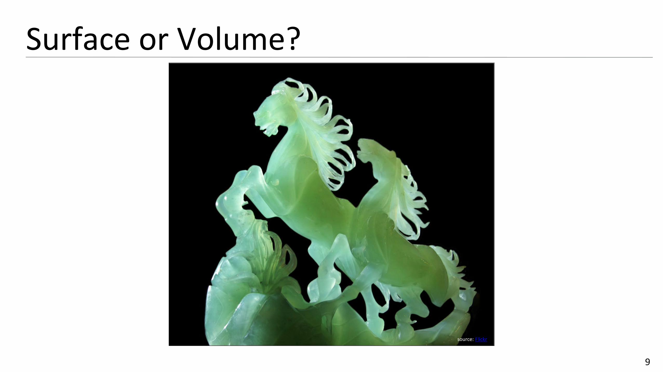
Scattering
17
http://coclouds.com

Defining Participating MediaTypically, we do not model particles of a medium explicitly (wouldn’t fit in memory, completely impractical to ray trace)
The properties are described statistically using various coefficients and densities- Conceptually similar idea as microfacet models
18

Defining Participating MediaHomogeneous:- Infinite or bounded by a surface or simple shape
19

Defining Participating MediaHeterogeneous (spatially varying coefficients):- Procedurally, e.g., using a noise function
- Simulation + volume discretization, e.g., a voxel grid
20

RadianceThe main quantity we are interested in for rendering is radiance
Previously: radiance remains constant along rays between surfaces
21

RadianceThe main quantity we are interested in for rendering is radiance
Now: radiance may change along rays between surfaces
22

Participating Media
23

Differential Beam
24
How much light is lost/gained along the differential beamdue to interactions of light with the medium?
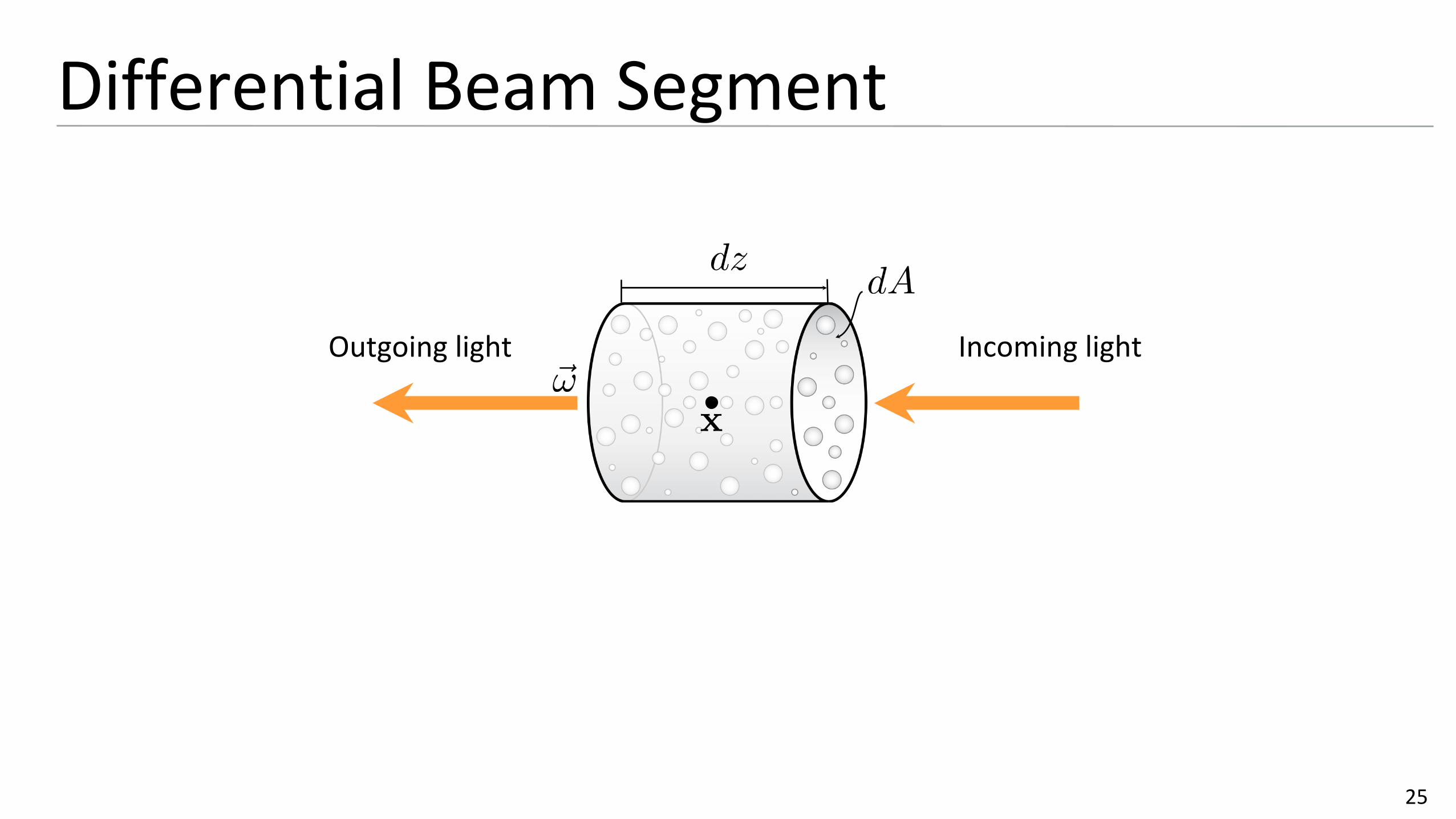
Differential Beam Segment
25
Incoming lightOutgoing light

Absorption
26
: absorption coefficient

Out-scattering
27
: scattering coefficient

In-scattering
28
: scattering coefficient
: in-scattered radiance

Emission
29
: emitted radiance
: absorption coefficient*Sometimes modeled without the absorption coefficient justby specifying a “source” term
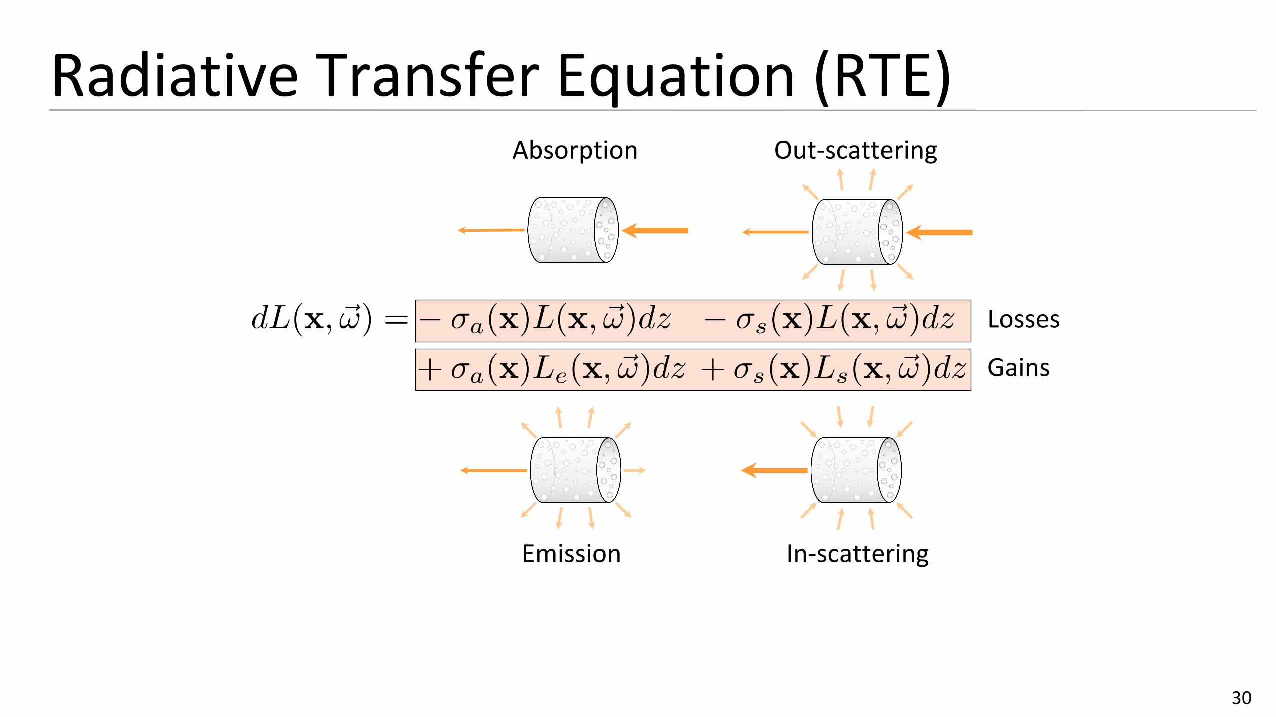
Gains
Losses
Radiative Transfer Equation (RTE)
30
Emission In-scattering
Out-scatteringAbsorption

Losses (Extinction)
31
: extinction coefficient: total loss of light per unit distance
Absorption Out-scattering
What about a beam with a finite length?

Extinction Along a Finite Beam
32
// Integrate along beam from 0 to z
// Exponentiate
// Assume constant 𝜎𝜎𝑡𝑡(𝐱𝐱), reorganize

Beer-Lambert Law
Radiance at distance z
Radiance at the beginningof the beam
Expresses the remaining radiance after traveling a finite distance through a medium with constant extinction coefficient
The fraction is referred to as the transmittance
Think of this as fractional visibility between points

distance
TransmittanceHomogeneous volume:
Heterogeneous volume (spatially varying 𝜎𝜎𝑡𝑡):
34
Optical thickness
5

TransmittanceHomogeneous volume:
Heterogeneous volume (spatially varying 𝜎𝜎𝑡𝑡):
Transmittance is multiplicative:
35
Optical thickness

Radiative Transfer Equation (RTE)
36
Emission In-scattering
Out-scatteringAbsorption

Volume Rendering Equation
37
Reduced (background) surface radiance

Volume Rendering Equation
38
Accumulated emitted radiance

Volume Rendering Equation
39
Accumulated in-scattered radiance

Volume Rendering Equation
40
Accumulated in-scattered radiance

Volume Rendering Equation
41

Scattering in Media

Phase Function 𝑓𝑓𝑝𝑝Describes distribution of scattered light
Analog of BRDF but for scattering in media
Integrates to unity (unlike BRDF)
43
*We will use the same convention that phase function direction vectors always point away from theshading point x. Many publications, however, use a different convention for phase functions, in whichdirection vectors “follow” the light, i.e. one direction points towards x and the other away from x. Whenreading papers, be sure to clarify the meaning of the vectors to avoid misinterpretation.
Why do we have this property?

Isotropic ScatteringUniform scattering, analogous to Lambertian BRDF
44
Where does this value come from?

Anisotropic ScatteringQuantifying anisotropy (𝑔𝑔, “average cosine”):
where:
𝑔𝑔 = 0 : isotropic scattering (on average)𝑔𝑔 > 0 : forward scattering𝑔𝑔 < 0 : backward scattering
45

Henyey-Greenstein Phase FunctionAnisotropic scattering
46

Henyey-Greenstein Phase FunctionAnisotropic scattering
47

Henyey-Greenstein Phase Function
48
Linear plot Log plot

Henyey-Greenstein Phase FunctionEmpirical phase function
Introduced for intergalactic dust
Very popular in graphics and other fields
49

Schlick’s Phase FunctionEmpirical phase function
Faster approximation of HG
50

Schlick’s Phase FunctionEmpirical phase function
Faster approximation of HG
51
HGSchlick

Lorenz-Mie ScatteringIf the diameter of scatterers is on the order of light wavelength, we cannot neglect the wave nature of light
Solution to Maxwell’s equations for scattering from any spherical dielectric particle
Explains many phenomena
Complicated:- Solution is an infinite analytic series
52

Lorenz-Mie Phase Function
53
Line
ar p
lots
Log plots
Sphere diameter Sphere diameter Sphere diameter
Data obtained from http://www.philiplaven.com/mieplot.htm

Rainbows
54

Murky atmosphereHazy atmosphere
Lorenz-Mie Approximations
55

Lorenz-Mie Approximations
56
Hazy atmosphere Murky atmosphere
johnib.wordpress.com srollinson.blogspot.com

Rayleigh ScatteringApproximation of Lorenz-Mie for tiny scatterers that are typically smaller than 1/10th the wavelength of visible light
Used for atmospheric scattering, gasses, transparent solids
Highly wavelength dependent
57

Rayleigh Phase Function
58
Scattering at right angles is half as likely as scattering forward or backward

Rayleigh Scattering
59
Wavelength
Index of refraction
Diameter of scatterersDensity of scatterers

Rayleigh Scattering
60

Examples
61
Dana Stephenson/Getty Images

Examples
62
Steam Smoke
Forward scattering Backward scattering

Examples
63
Isotropic scattering

Examples
64
Forward scattering

Atmosphere
Why is the Sky Blue?
65
Earth

Atmosphere
Why is the Sunset Red?
66
Earth

Rayleigh Scattering
67

Media Properties (Recap)Given:- Absorption coefficient
- Scattering coefficient
- Phase function
Derived:- Extinction coefficient
- Albedo
- Mean-free path
- Transmittance
68

Homogeneous Isotropic MediumGiven:- Absorption coefficient
- Scattering coefficient
- Phase function
Derived:- Extinction coefficient
- Albedo
- Mean-free path
- Transmittance
69

Crepuscular Rays
71
source: wikipedia

Anti-Crepuscular Rays
72
source: wikipedia

Crepuscular rays from space
73
source: wikipedia

Solving the Volume Rendering Equation

Complexity Progressionhomogeneous vs. heterogeneous
scattering- none
- fake ambient
- single
- multiple
75

Accumulated in-scattered radiance
Attenuated background radiance
Accumulated emitted radiance
Volume Rendering Equation
76

Attenuated background radiance
Purely absorbing media

Homogeneous medium
Participating Media
80

Homogeneous Ambient MediaAssume in-scattered radiance is an ambient constant:
82

Homogeneous Ambient MediaAssume in-scattered radiance is an ambient constant:
83
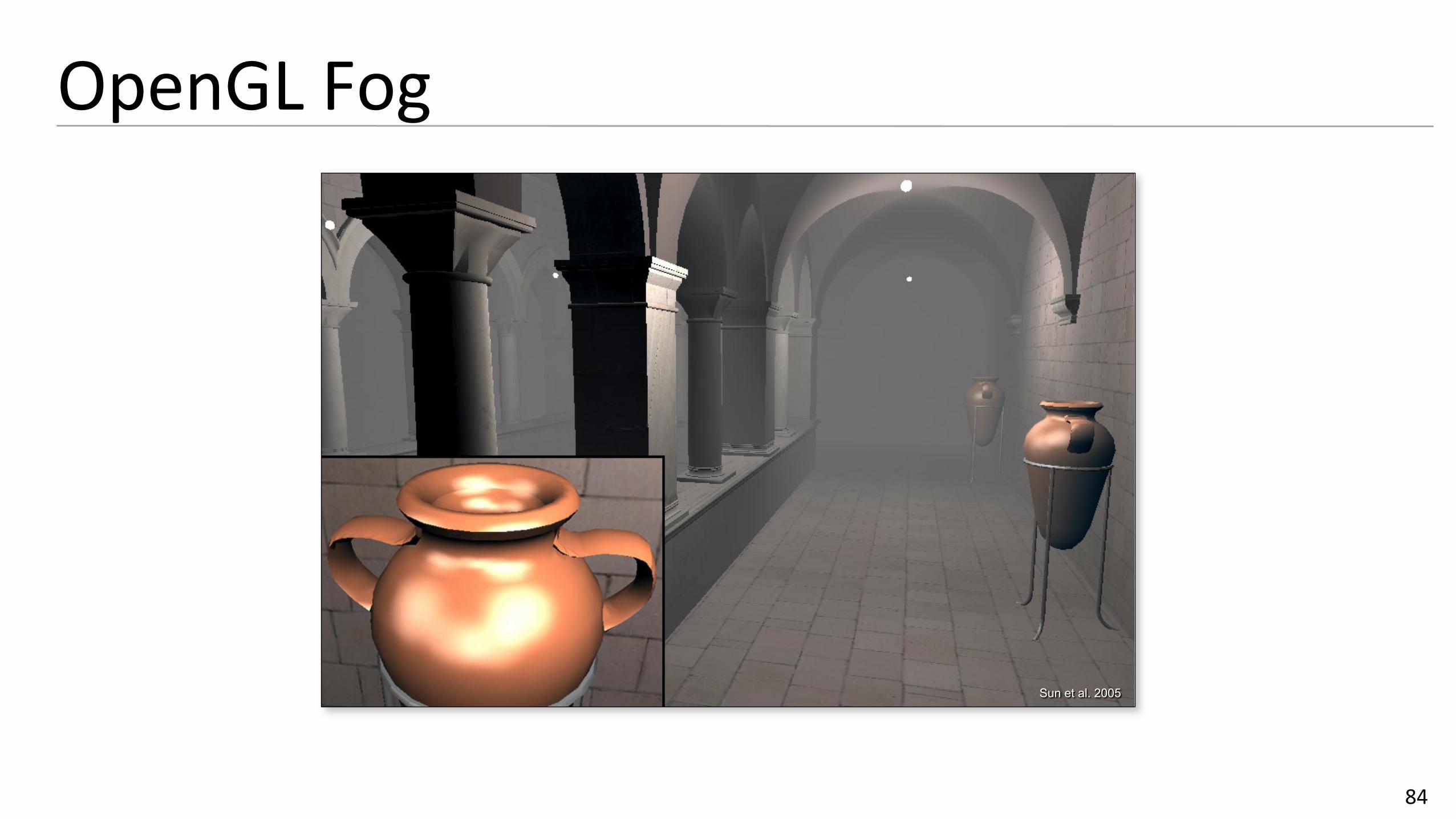
OpenGL Fog
84
Sun et al. 2005

OpenGL Clear Day
85
Sun et al. 2005

Fog
86

Volume Rendering Equation
93
Accumulated in-scattered radiance

In-scattered Radiance
Single scattering- 𝐿𝐿𝑖𝑖 arrives directly from a light source (direct illum.)
i.e.:
Multiple scattering- 𝐿𝐿𝑖𝑖 arrives through multiple bounces (indirect illum.)
94
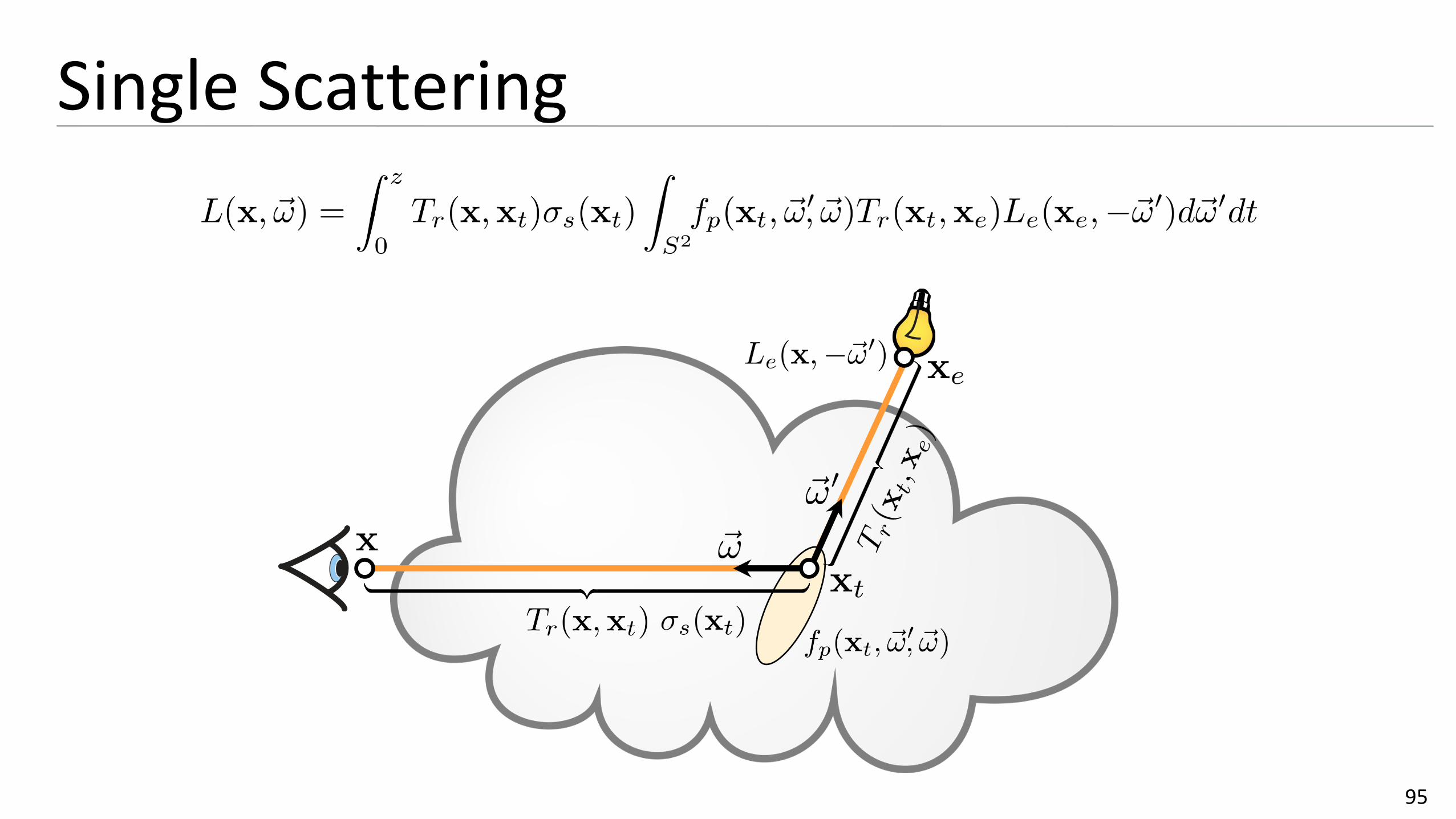
Single Scattering
95
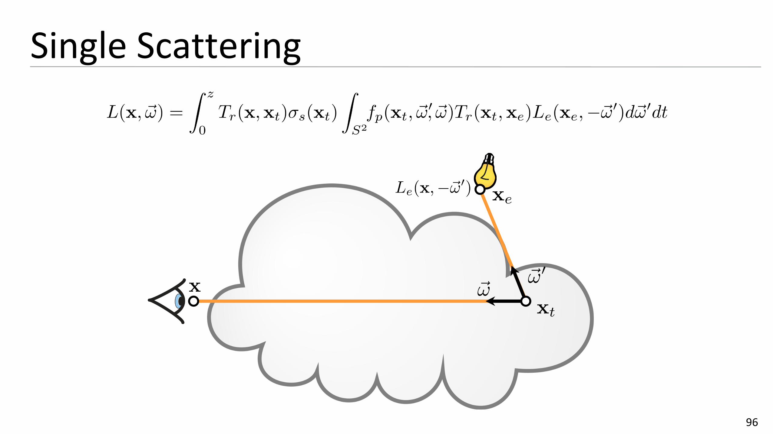
Single Scattering
96

Single Scattering
97

Single Scattering
98

Single Scattering
(Semi-)analytic solutions:- Sun et al. [2005]
- Pegoraro et al. [2009, 2010]
Numerical solutions:- Ray-marching
- Equiangular sampling
99

Analytic Single Scattering
Assumptions:- Homogeneous medium
- Point or spot light
- Relatively simple phase function
- No occlusion
100

OpenGL Fog
101
Sun et al. 2005

Analytic Single Scattering
102
Sun et al. 2005

Analytic Single Scattering
104
Pegoraro et al. 2010Pegoraro et al. 2009

Analytic Single Scattering
107
No shadows, implementation nightmare, computationally intensive...Let’s try brute force!

Ray-Marching
108
Approximate with Riemann sum

Ray-Marching
109

Ray-Marching
110

Ray-Marching
111
Homogeneous volume:

Ray-Marching
112
Heterogeneous volume:
Assume constant extinctionalong each segment
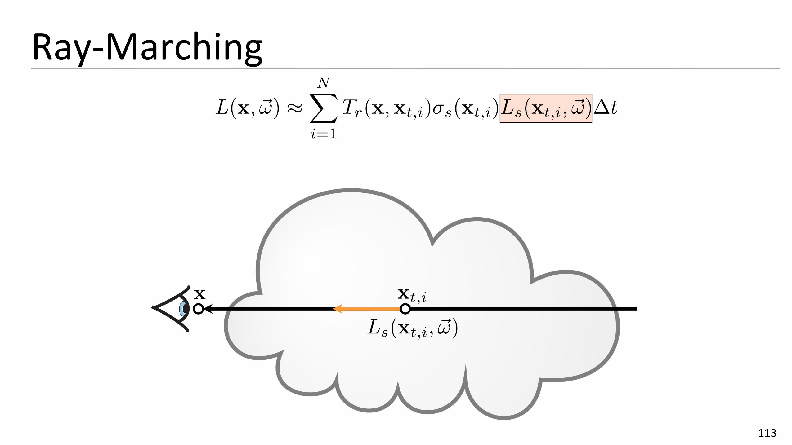
Ray-Marching
113

Ray-Marching
114

Ray-Marching
115
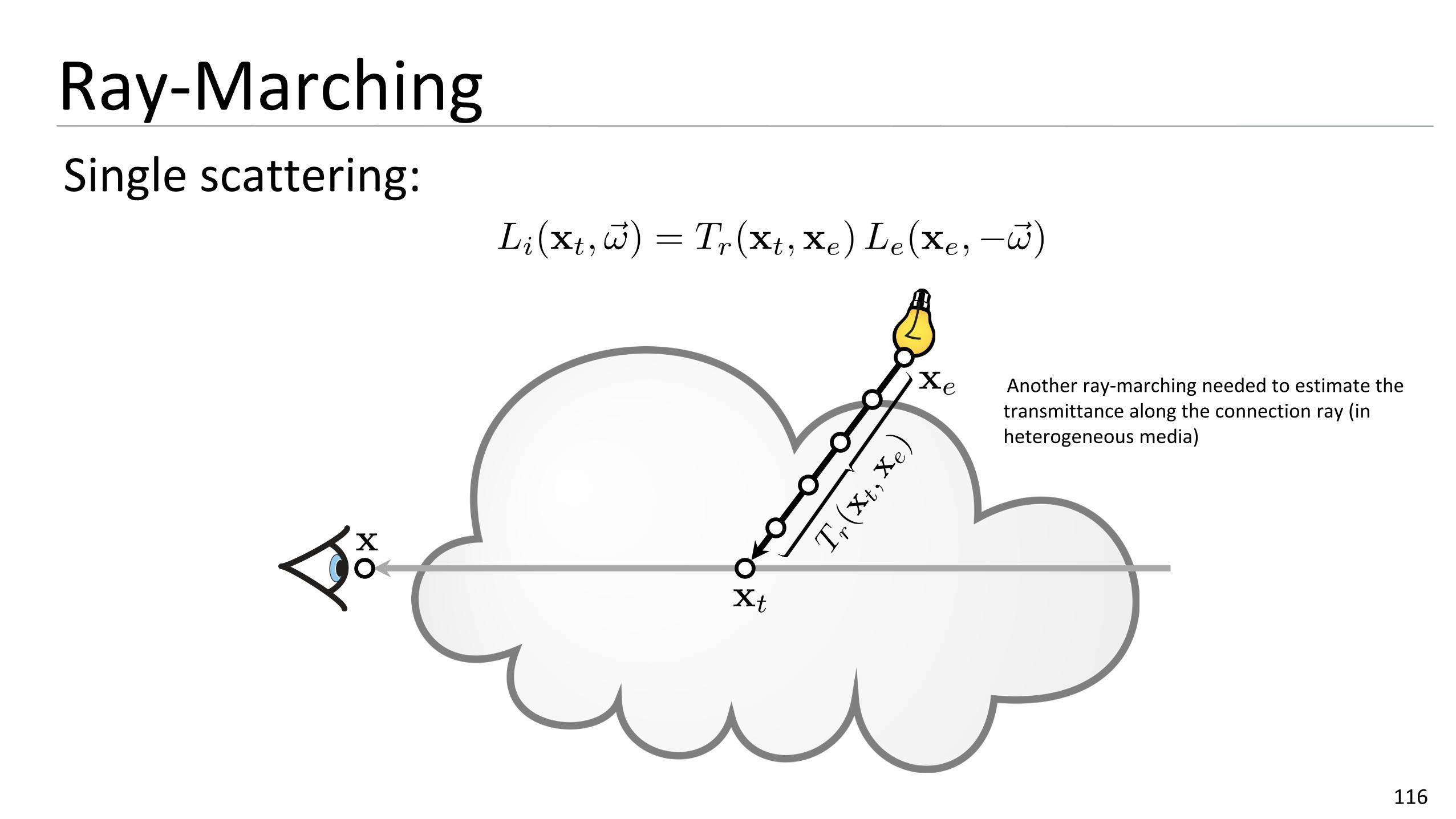
Ray-MarchingSingle scattering:
116
Another ray-marching needed to estimate the transmittance along the connection ray (in heterogeneous media)

Ray-Marching in Heterogeneous MediaMarching towards the light source- Connections are expensive, many, and uniformly distributed along
the primary ray
117

Piece-wise approximation of
Decoupled Transmittance and In-scattering1. Ray-march and cache transmittance- Choose step-size w.r.t. frequency content to accurately capture
variations
118

Decoupled Transmittance and In-scattering2. Estimate in-scattering using MC integration
- Distribute samples ∝ (part of) the integrand
119

Decoupled Transmittance and In-scattering2. Estimate in-scattering using MC integration
- Distribute samples ∝ (part of) the integrand
120

Decoupled Transmittance and In-scattering2. Estimate in-scattering using MC integration
- Distribute samples ∝ (part of) the integrand
: distance to light
121

Decoupled Transmittance and In-scattering2. Estimate in-scattering using MC integration
- Distribute samples ∝ (part of) the integrand
122
: distance to light

Decoupled Transmittance and In-scattering2. Estimate in-scattering using MC integration
- Distribute samples ∝ (part of) the integrand
123
: distance to light

Decoupled Transmittance and In-scattering2. Estimate in-scattering using MC integration
- Distribute samples ∝ (part of) the integrand
Equi-angularsampling
[Kulla and Fajardo 2012]
124
: distance to light

Decoupled Transmittance and In-scattering
125
Ray-marching Equiangular sampling
Images courtesy of Kulla and Fajardo

Multiple BouncesSame concept as in recursive Monte Carlo ray tracing, but taking into account volumetric scattering
Exponential growth:
126
...

Visual Break
127
Single scattering Multiple scattering

Volumetric Path Tracing

Volumetric Path TracingMotivation:- Same as with standard path tracing: avoid the exponential growth
Paths can:- Reflect/refract off surfaces
- Scatter inside a volume
129

Accumulated in-scattered radiance
Attenuated background radiance
Accumulated emitted radiance
Volume Rendering Equation
130

Attenuated background radiance
Accumulated emitted + in-scattered radiance
Volume Rendering Equation
131

Volume Rendering Equation
132

1-Sample Monte Carlo Estimator
133
- probability density of distance t
- probability of exceeding distance z
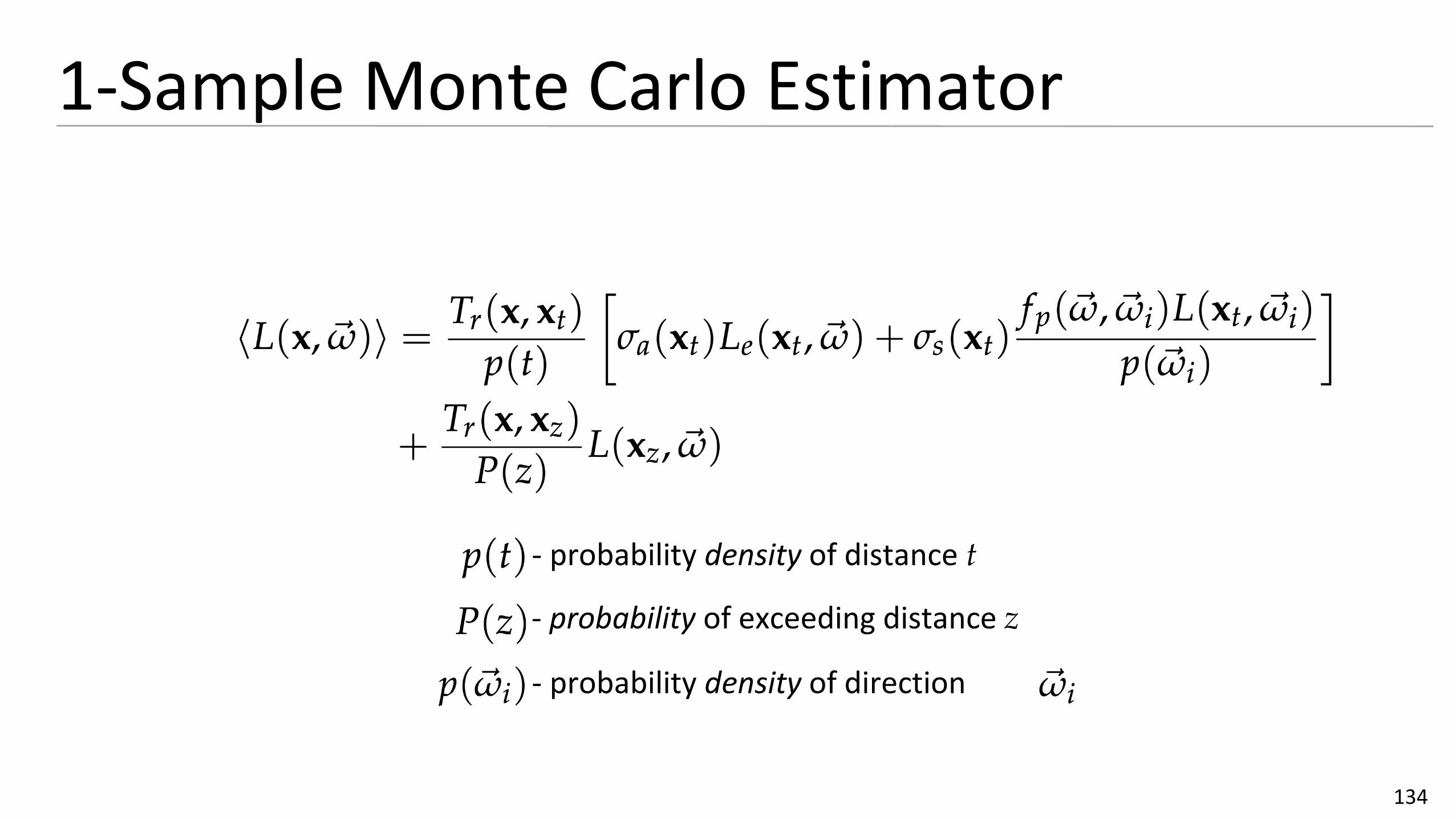
1-Sample Monte Carlo Estimator
134
- probability density of distance t
- probability of exceeding distance z
- probability density of direction
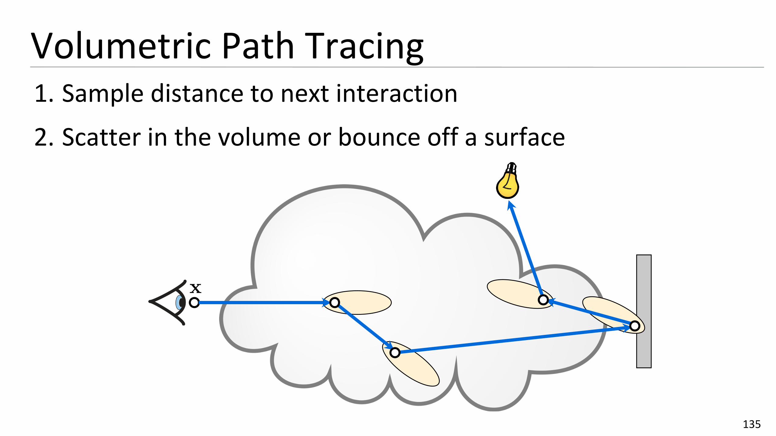
Volumetric Path Tracing1. Sample distance to next interaction
2. Scatter in the volume or bounce off a surface
135

Volumetric Path Tracing with NEE
136

Sampling the Phase FunctionIsotropic:- Uniform sphere sampling
Henyey-Greenstein:- Using the inversion method we can derive
- PDF is the value of the HG phase function
137

Free-path SamplingFree-path (or free-flight distance):- Distance to the next interaction within the medium
- Dense media (e.g. milk): short mean-free path
- Thin media (e.g. atmosphere): long mean-free path
Ideally, we want to sample proportional to (part of) integrand, e.g. transmittance:
138
simplified notation for brevity

Free-path SamplingHomogeneous media: - PDF:
- CDF:
- Inverted CDF:
139

Free-path SamplingHomogeneous media:
Recipe:- Generate random number
- Sample distance
- Compute PDF
140

Free-path SamplingHomogeneous media:
Recipe:- Generate random number
- Sample distance
- Compute PDF
141
Surface hit before reaching
Note: This is now a probability, not a probability density!

Volumetric PT for Homogeneous VolumesColor vPT(x, ω)tmax = nearestSurface(x, ω)t = -log(1 - randf()) / σt // Sample free pathif t < tmax: // Volume interactionx += t * ωpdf_t = σt * exp(-σt * t)(ω’, pdf_ω’) = samplePF(ω)return Tr(t) / pdf_t * (σa * Le(x, ω) + σs * PF(ω, ω’) * vPT(x, ω’) / pdf_ω’)else: // Surface interactionx += tmax * ωPr_tmax = exp(-σt * tmax)(ω’, pdf_ω’) = sampleBRDF(n, ω)return Tr(tmax) / Pr_tmax * (Le(x, ω) + BRDF(ω, ω’) * vPT(x, ω’) / pdf_ω’)
142

Volumetric PT for Homogeneous VolumesColor vPT(x, ω)tmax = nearestSurface(x, ω)t = -log(1 - randf()) / σt // Sample free pathif t < tmax: // Volume interactionx += t * ωpdf_t = σt * exp(-σt * t)(ω’, pdf_ω’) = samplePF(ω)// Note: transmittance and PF cancel out with PDFs except for a constant factor 1/σtreturn Tr(t) / pdf_t * (σa * Le(x, ω) + σs * PF(ω, ω’) * vPT(x, ω’) / pdf_ω’)else: // Surface interactionx += tmax * ωPr_tmax = exp(-σt * tmax)(ω’, pdf_ω’) = sampleBRDF(n, ω)// Note: transmittance and prob of sampling the distance cancel outreturn Tr(tmax) / Pr_tmax * (Le(x, ω) + BRDF(ω, ω’) * vPT(x, ω’) / pdf_ω’)
143

Volumetric PT for Homogeneous VolumesColor vPT(x, ω)tmax = nearestSurface(x, ω)t = -log(1 - randf()) / σt // Sample free pathif t < tmax: // Volume interactionx += t * ωpdf_t = σt * exp(-σt * t)(ω’, pdf_ω’) = samplePF(ω)// Note: transmittance and PF cancel out with PDFs except for a constant factor 1/σtreturn σa/σt * Le(x, ω) + σs/σt * vPT(x, ω’)else: // Surface interactionx += tmax * ωPr_tmax = exp(-σt * tmax)(ω’, pdf_ω’) = sampleBRDF(n, ω)// Note: transmittance and prob of sampling the distance cancel outreturn Le(x, ω) + BRDF(ω, ω’) * vPT(x, ω’) / pdf_ω’
144

What about heterogeneous media?
145

Free-path SamplingHeterogeneous media: - Closed-form solutions exist only for simple media
• e.g. linearly or exponentially varying extinction
- Other solutions:
• Regular tracking (3D DDA)
• Ray marching
• Delta tracking
146

Free-path SamplingHow to sample the flight distance to the next interaction?
147
Random variable representing flight distance
CDF
Partition of unity
Recipe for generating samples

Free-path Sampling
148
Probability density function (PDF)
Inverted cumulative distr. function (CDF-1)Approaches for finding t:1) ANALYTIC (closed-form CDF-1)2) SEMI-ANALYTIC (regular tracking)3) APPROXIMATE (ray marching)
Solve for t
Cumulative distribution function (CDF)

For piecewise-simple (e.g. piecewise-constant), summation replaces integration
Regular Tracking (Semi-Analytic)
149
(Hierarchical) voxel grid
Start
SampledcollisionLHS=RHS
LHS > RHS

Find the collision distance approximately
Ray Marching
151
(Hierarchical) voxel grid
Start
SampledcollisionLHS=RHS
LHS > RHSConstant step

Find the collision distance approximately
Ray Marching
152
General volume
Constant step
Start
SampledcollisionLHS=RHS
LHS > RHS

Find the collision distance approximately
Ray Marching
153
General volume
Ignored thin features = bias
Start
Constant step
SampledcollisionLHS=RHS
LHS > RHS

Free-path Sampling
156
‣ Efficient & simple, limited to few volumes
‣ Iterative, inefficient if free paths cross many boundaries
‣ Iterative, inaccurate (or inefficient) for media with high frequencies
‣ Simple volumes(e.g. homogeneous)
‣ Piecewise-simple volumes
‣ Any volume
‣ Unbiased ‣ Unbiased ‣ Biased
ANALYTIC CDF-1 REGULAR TRACKING RAY MARCHING
Common approach: sample optical thickness, find corresponding distance

Delta Tracking(a.k.a. Woodcock tracking, pseudo scattering, hole tracking, null-collision method,…)

Delta tracking ideaAdd FICTITIOUS MATTER to homogenize medium
- albedo: 𝛼𝛼(𝐱𝐱) = 1
- phase function: 𝑓𝑓𝑝𝑝(𝜔𝜔
,𝜔𝜔 ′) = 𝛿𝛿(𝜔𝜔
− 𝜔𝜔
′)
159
Fictitious particle
Incidentlight
Outgoinglight
Presence of fictitious matterdoes not impact light transport

Homogenization
160
Volume bounds
Real particle

Volume bounds
Homogenization
161
Fictitious particle
Real particle

Volume bounds
Homogenization
162
Fictitious particle
Real particle

Volume bounds
Homogenization
163
Fictitious particle
Real particle

Volume bounds
Homogenization
164
Fictitious particle
Real particle

Volume bounds
Homogenization
165
Fictitious particle
Real particle

Volume bounds
Homogenization
166
Fictitious particle
Real particle

Volume bounds
Homogenization
167
Fictitious particle
Real particle

Volume bounds
Homogenization
168
Fictitious particle
Real particle

Volume bounds
Homogenization
169
Fictitious particle
Real particle

Volume bounds
Homogenization
170
Fictitious particle
Real particle

Homogenization
171
Volume bounds
Real particle

Stochastic Sampling
172
Volume bounds
Real medium

Stochastic Sampling
173
Volume bounds
Real medium
Majorant
Fictitious medium

Stochastic Sampling
DistanceEx
tinct
ion
Tentativecollision
Majorant

Stochastic Sampling
175
DistanceEx
tinct
ion
Tentativecollision
Majorant
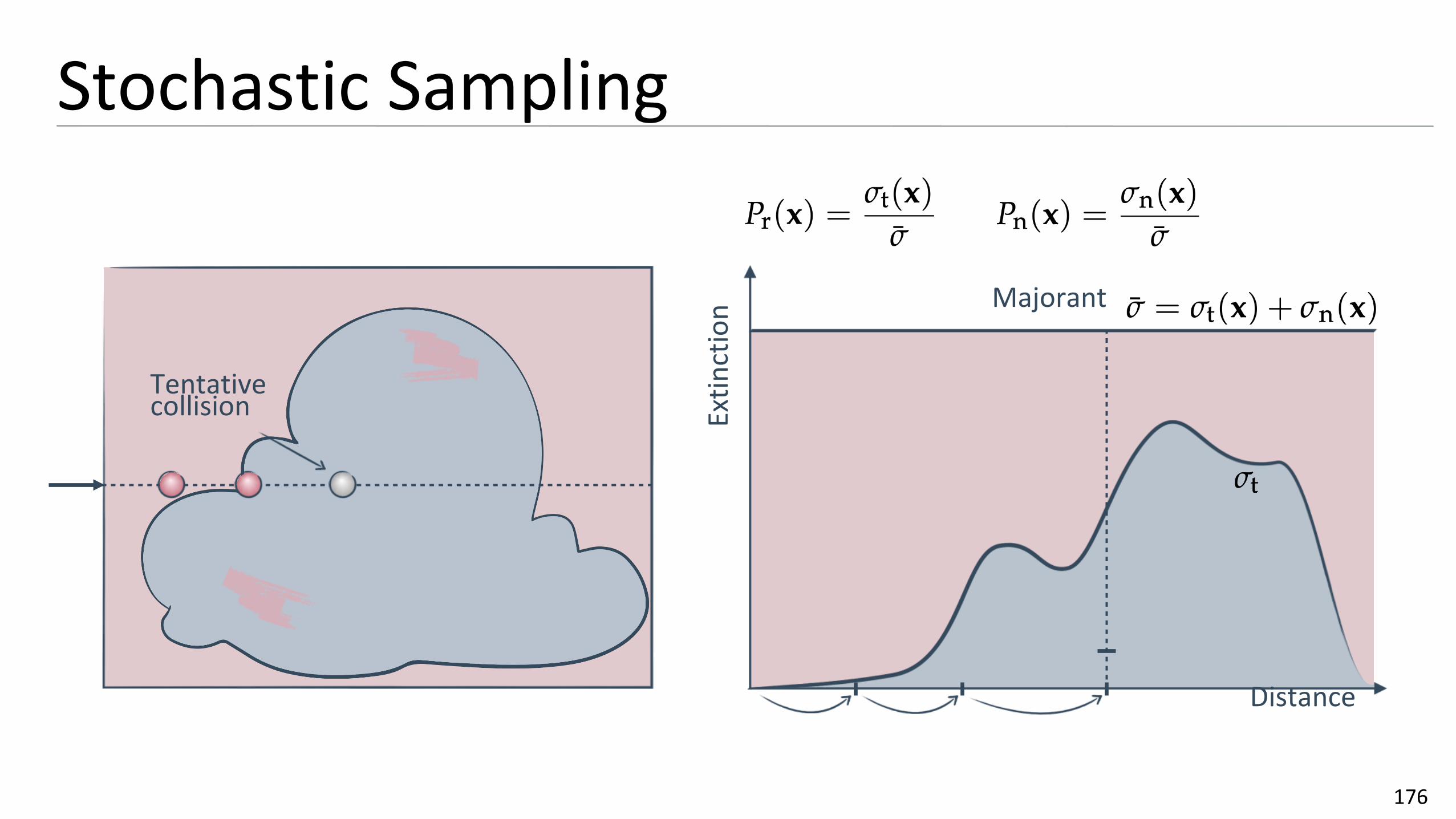
Stochastic Sampling
176
DistanceEx
tinct
ion
Tentativecollision
Majorant

Stochastic Sampling
177
DistanceEx
tinct
ion
Realcollision
Sampled free path
Majorant

Impact of Majorant
178
DistanceEx
tinct
ion
Sampled free path
Majorant

Impact of Majorant
179
DistanceEx
tinct
ion
Tight majorant = GOOD(few rejected collisions)
Sampled free path
Majorant

Impact of Majorant
180
Distance
Loose majorant = BAD(many expensive rejected collisions)
Sampled free pathEx
tinct
ion
Majorant

Delta Trackingvoid preprocess()
majorant = findMaximumExtinction()
void sampleFreePath(x, ω)
t = 0
do:
// Sample distance to next tentative collision
t += -ln(1 - randf()) / majorant
// Compute probability of a real collision
Pr = getExtinction(x + t*ω) / majorant
while Pr < randf()
return t
181

Delta Tracking SummaryUnbiased, see [Coleman 68] for a proof
182

Delta Tracking SummaryUnbiased, see [Coleman 68] for a proof
Majorant extinction- defines the combined homogeneous volume
- must bound the real extinction
- loose majorants lead to many fictitious collisions
183