Rendering Aurora

Tao, Dutaodu@stanford.edu

Wenlong, Luwenlongl@stanford.edu

June 11, 2014

1 Introduction

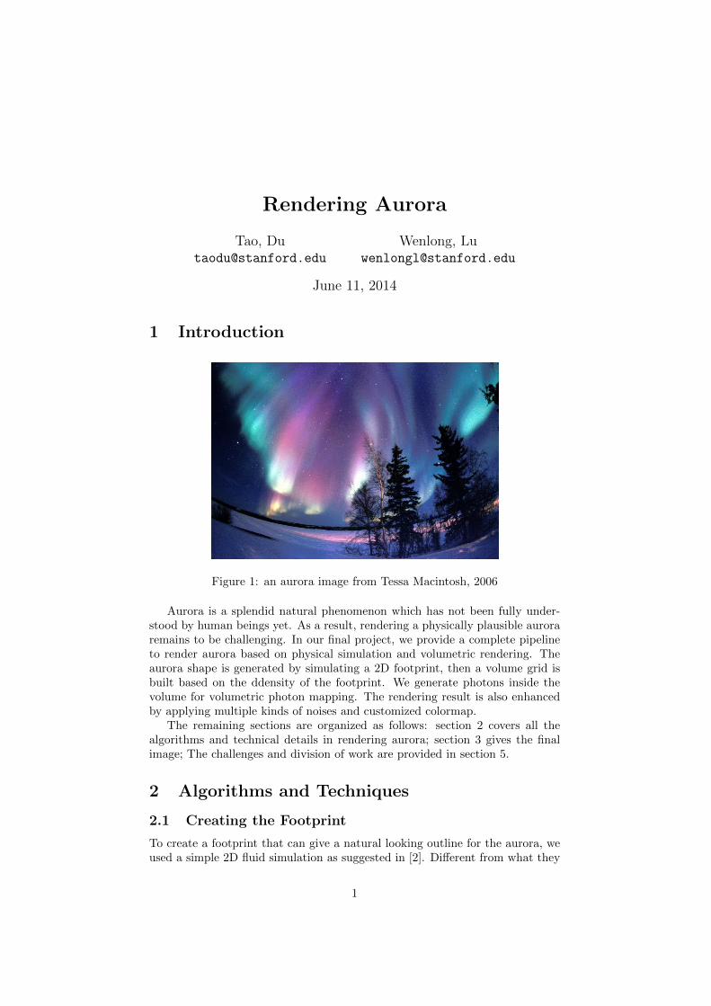
Figure 1: an aurora image from Tessa Macintosh, 2006

Aurora is a splendid natural phenomenon which has not been fully under-stood by human beings yet. As a result, rendering a physically plausible auroraremains to be challenging. In our final project, we provide a complete pipelineto render aurora based on physical simulation and volumetric rendering. Theaurora shape is generated by simulating a 2D footprint, then a volume grid isbuilt based on the ddensity of the footprint. We generate photons inside thevolume for volumetric photon mapping. The rendering result is also enhancedby applying multiple kinds of noises and customized colormap.

The remaining sections are organized as follows: section 2 covers all thealgorithms and technical details in rendering aurora; section 3 gives the finalimage; The challenges and division of work are provided in section 5.

2 Algorithms and Techniques

2.1 Creating the Footprint

To create a footprint that can give a natural looking outline for the aurora, weused a simple 2D fluid simulation as suggested in [2]. Different from what they

1

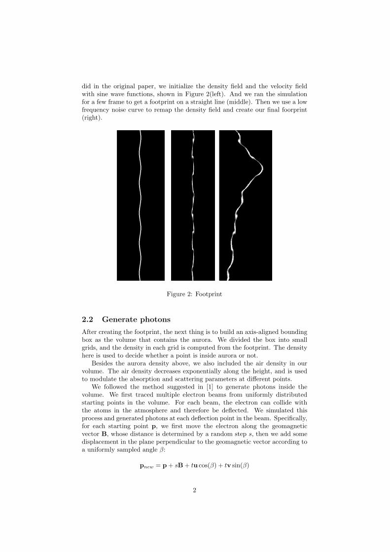
did in the original paper, we initialize the density field and the velocity fieldwith sine wave functions, shown in Figure 2(left). And we ran the simulationfor a few frame to get a footprint on a straight line (middle). Then we use a lowfrequency noise curve to remap the density field and create our final foorprint(right).

Figure 2: Footprint

2.2 Generate photons

After creating the footprint, the next thing is to build an axis-aligned boundingbox as the volume that contains the aurora. We divided the box into smallgrids, and the density in each grid is computed from the footprint. The densityhere is used to decide whether a point is inside aurora or not.

Besides the aurora density above, we also included the air density in ourvolume. The air density decreases exponentially along the height, and is usedto modulate the absorption and scattering parameters at different points.

We followed the method suggested in [1] to generate photons inside thevolume. We first traced multiple electron beams from uniformly distributedstarting points in the volume. For each beam, the electron can collide withthe atoms in the atmosphere and therefore be deflected. We simulated thisprocess and generated photons at each deflection point in the beam. Specifically,for each starting point p, we first move the electron along the geomagneticvector B, whose distance is determined by a random step s, then we add somedisplacement in the plane perpendicular to the geomagnetic vector according toa uniformly sampled angle β:

pnew = p + sB + tu cos(β) + tv sin(β)

2

where u, v and B form a Cartesian coordinate system. The parameter tdetermines how much the electron deviates from the geomagnetic vector. Wecompute t by sampling in the angle α between pnew − p and B:

tanα =t

s

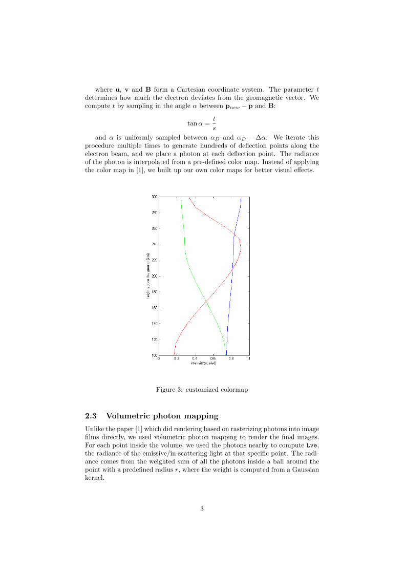
and α is uniformly sampled between αD and αD − ∆α. We iterate thisprocedure multiple times to generate hundreds of deflection points along theelectron beam, and we place a photon at each deflection point. The radianceof the photon is interpolated from a pre-defined color map. Instead of applyingthe color map in [1], we built up our own color maps for better visual effects.

Figure 3: customized colormap

2.3 Volumetric photon mapping

Unlike the paper [1] which did rendering based on rasterizing photons into imagefilms directly, we used volumetric photon mapping to render the final images.For each point inside the volume, we used the photons nearby to compute Lve,the radiance of the emissive/in-scattering light at that specific point. The radi-ance comes from the weighted sum of all the photons inside a ball around thepoint with a predefined radius r, where the weight is computed from a Gaussiankernel.

3

Both photon generating and volumetric photon mapping are implemented ina custom class AuroraDensity, which is inherited from VolumeRegion in pbrt.

2.4 Adding Noise

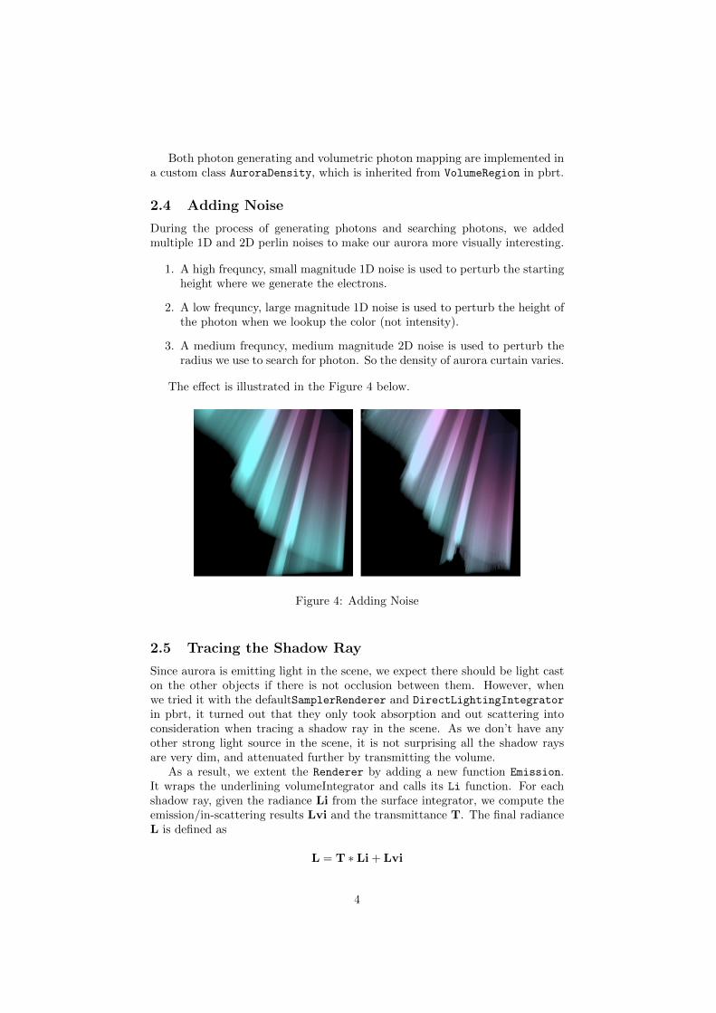
During the process of generating photons and searching photons, we addedmultiple 1D and 2D perlin noises to make our aurora more visually interesting.

1. A high frequncy, small magnitude 1D noise is used to perturb the startingheight where we generate the electrons.

2. A low frequncy, large magnitude 1D noise is used to perturb the height ofthe photon when we lookup the color (not intensity).

3. A medium frequncy, medium magnitude 2D noise is used to perturb theradius we use to search for photon. So the density of aurora curtain varies.

The effect is illustrated in the Figure 4 below.

Figure 4: Adding Noise

2.5 Tracing the Shadow Ray

Since aurora is emitting light in the scene, we expect there should be light caston the other objects if there is not occlusion between them. However, whenwe tried it with the defaultSamplerRenderer and DirectLightingIntegrator

in pbrt, it turned out that they only took absorption and out scattering intoconsideration when tracing a shadow ray in the scene. As we don’t have anyother strong light source in the scene, it is not surprising all the shadow raysare very dim, and attenuated further by transmitting the volume.

As a result, we extent the Renderer by adding a new function Emission.It wraps the underlining volumeIntegrator and calls its Li function. For eachshadow ray, given the radiance Li from the surface integrator, we compute theemission/in-scattering results Lvi and the transmittance T. The final radianceL is defined as

L = T ∗ Li + Lvi

4

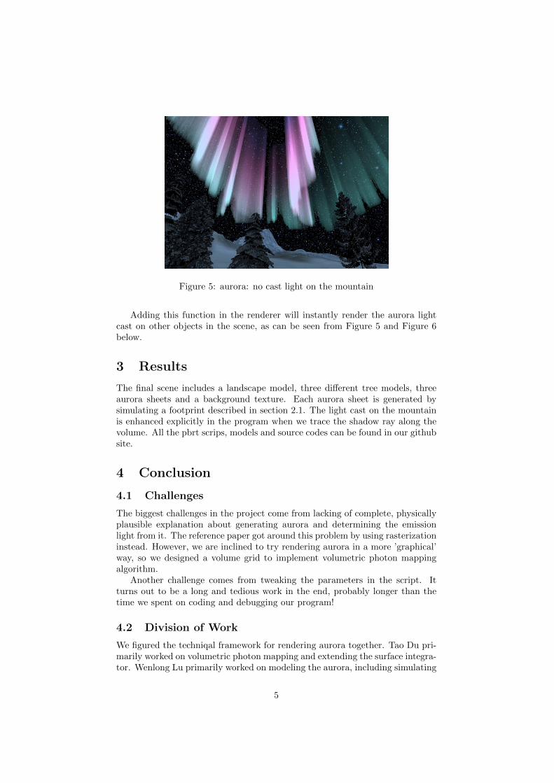
Figure 5: aurora: no cast light on the mountain

Adding this function in the renderer will instantly render the aurora lightcast on other objects in the scene, as can be seen from Figure 5 and Figure 6below.

3 Results

The final scene includes a landscape model, three different tree models, threeaurora sheets and a background texture. Each aurora sheet is generated bysimulating a footprint described in section 2.1. The light cast on the mountainis enhanced explicitly in the program when we trace the shadow ray along thevolume. All the pbrt scrips, models and source codes can be found in our githubsite.

4 Conclusion

4.1 Challenges

The biggest challenges in the project come from lacking of complete, physicallyplausible explanation about generating aurora and determining the emissionlight from it. The reference paper got around this problem by using rasterizationinstead. However, we are inclined to try rendering aurora in a more ’graphical’way, so we designed a volume grid to implement volumetric photon mappingalgorithm.

Another challenge comes from tweaking the parameters in the script. Itturns out to be a long and tedious work in the end, probably longer than thetime we spent on coding and debugging our program!

4.2 Division of Work

We figured the techniqal framework for rendering aurora together. Tao Du pri-marily worked on volumetric photon mapping and extending the surface integra-tor. Wenlong Lu primarily worked on modeling the aurora, including simulating

5

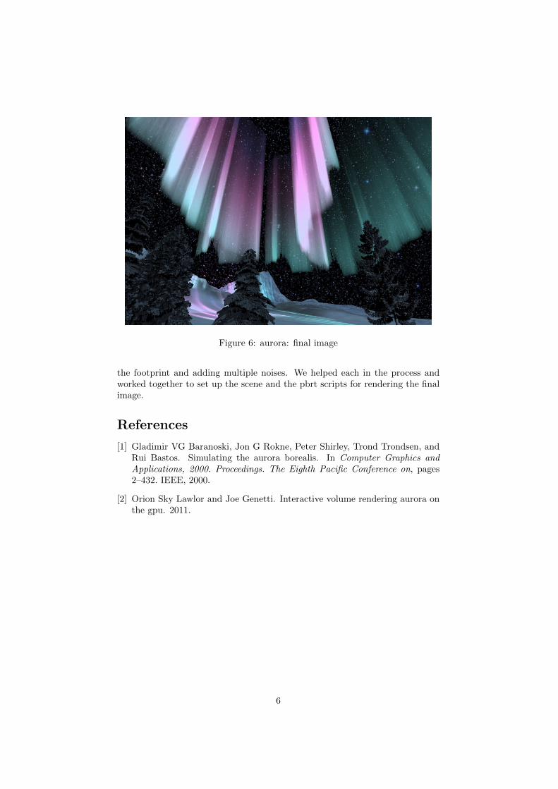
Figure 6: aurora: final image

the footprint and adding multiple noises. We helped each in the process andworked together to set up the scene and the pbrt scripts for rendering the finalimage.

References

[1] Gladimir VG Baranoski, Jon G Rokne, Peter Shirley, Trond Trondsen, andRui Bastos. Simulating the aurora borealis. In Computer Graphics andApplications, 2000. Proceedings. The Eighth Pacific Conference on, pages2–432. IEEE, 2000.

[2] Orion Sky Lawlor and Joe Genetti. Interactive volume rendering aurora onthe gpu. 2011.

6