Renato Bichara Vieira Thermography Applied to the … Bichara Vieira Thermography Applied to the...
139
Renato Bichara Vieira Thermography Applied to the Study of Fatigue in Polycarbonate Dissertação de Mestrado Thesis presented to the Programa de Pós-Graduação em Engenharia Mecânica of the Departamento de Engenharia Mecânica do Centro Técnico Científico da PUC-Rio, as partial fulfillment of the requirements for the degree of Mestre. Advisor: Prof. José Luiz de França Freire Rio de Janeiro April 2016
Transcript of Renato Bichara Vieira Thermography Applied to the … Bichara Vieira Thermography Applied to the...
Renato Bichara Vieira
Thermography Applied to the Study of
Fatigue in Polycarbonate
Dissertação de Mestrado
Thesis presented to the Programa de Pós-Graduação em Engenharia Mecânica of the Departamento de Engenharia Mecânica do Centro Técnico Científico da PUC-Rio, as partial fulfillment of the requirements for the degree of Mestre.
Advisor: Prof. José Luiz de França Freire
Rio de Janeiro April 2016
DBD
PUC-Rio - Certificação Digital Nº 1412756/CA

Renato Bichara Vieira
Thermography Applied to the Study of
Fatigue in Polycarbonate
Thesis presented to the Programa de Pós-Graduação em Engenharia Mecânica of the Departamento de Engenharia Mecânica do Centro Técnico Científico da PUC-Rio, as partial fulfillment of the requirements for the degree of Mestre.
Prof. José Luiz de França Freire Advisor
Departamento de Engenharia Mecânica – PUC-Rio
Prof. Jaime Tupiassú Pinho de Castro Departamento de Engenharia Mecânica – PUC-Rio
Prof. Sergio Damasceno Soares
Centro de Pesquisas da PETROBRAS - CENPES
Prof. Arthur Martins Barbosa Braga Departamento de Engenharia Mecânica – PUC-Rio
Prof. Marcio da Silveira Carvalho Coordenador Setorial do Centro Técnico Científico – PUC-Rio
Rio de Janeiro, Abril, 2016
DBD
PUC-Rio - Certificação Digital Nº 1412756/CA
All rights reserved.
Renato Bichara Vieira
Graduated in mechanical engineering in 2013 at the Pontifical
Catholic University of Rio de Janeiro. Worked since then in the
area of experimental stress analysis, specifically with the
various applications of thermography.
Ficha Catalográfica
Vieira, Renato Bichara
Thermography applied to the study of fatigue in
polycarbonate. / Renato Bichara Vieira; orientador: José Luiz
de França Freire. – 2016.
139 f. : il.(color.) ; 30 cm
Dissertação (mestrado)-Pontifícia Universidade Católica do Rio de Janeiro, Departamento de Engenharia Mecânica, 2016.
Inclui Bibliografia
1. Engenharia mecânica – Teses. 2. Termografia
Infravermelha. 3. Fadiga. 4. Policarbonato. 5. Análise
Termoelástica de Tensões. 6. Método Termográfico. 7. Fator
de Concentração de Tensões. 8. Limite de Fadiga. 9. Curva
de Wöhler. 10. Fator de Intensidade de Tensões. 11. Lei de
Paris. I. Freire, José Luiz de França. II. Pontifícia
Universidade Católica do Rio de Janeiro. Departamento de
Engenharia Mecânica. III. Título.
CDD: 621
DBD
PUC-Rio - Certificação Digital Nº 1412756/CA

Acknowledgments
I would like to thank my advisor Professor José Luiz de França Freire for all his
teachings, not only academic, but for all the life lessons as well.
I have to thank CNPq (Conselho Nacional de Desenvolvimento Científico e
Tecnológico) and FAPERJ (Fundação de Amparo à Pesquisa do Estado do Rio
de Janeiro) for their financial support, through the scholarships I was awarded.
I want to thank my family, especially my mother Thais and my father Ronaldo, for
all the unconditional support, love and help they provided me. They are my
inspiration and my reference.
Furthermore, I would like to thank my laboratory colleagues Felipe, Jesus, Jorge,
Marco and Vitor for making the process less straining. A special thanks goes to
Giancarlo, for the indispensable help during most of the experiments.
I have to thank ITUC, in special Adrian and Ana Rosa, for the support during some
of the experiments and for letting me use their equipment.
Finally, I like to give a big thanks to my friends, who helped me indirectly in the
process of getting my master’s degree. They are one major pillar on which I support
my life. Each one of them know who they are.
DBD
PUC-Rio - Certificação Digital Nº 1412756/CA
Abstract
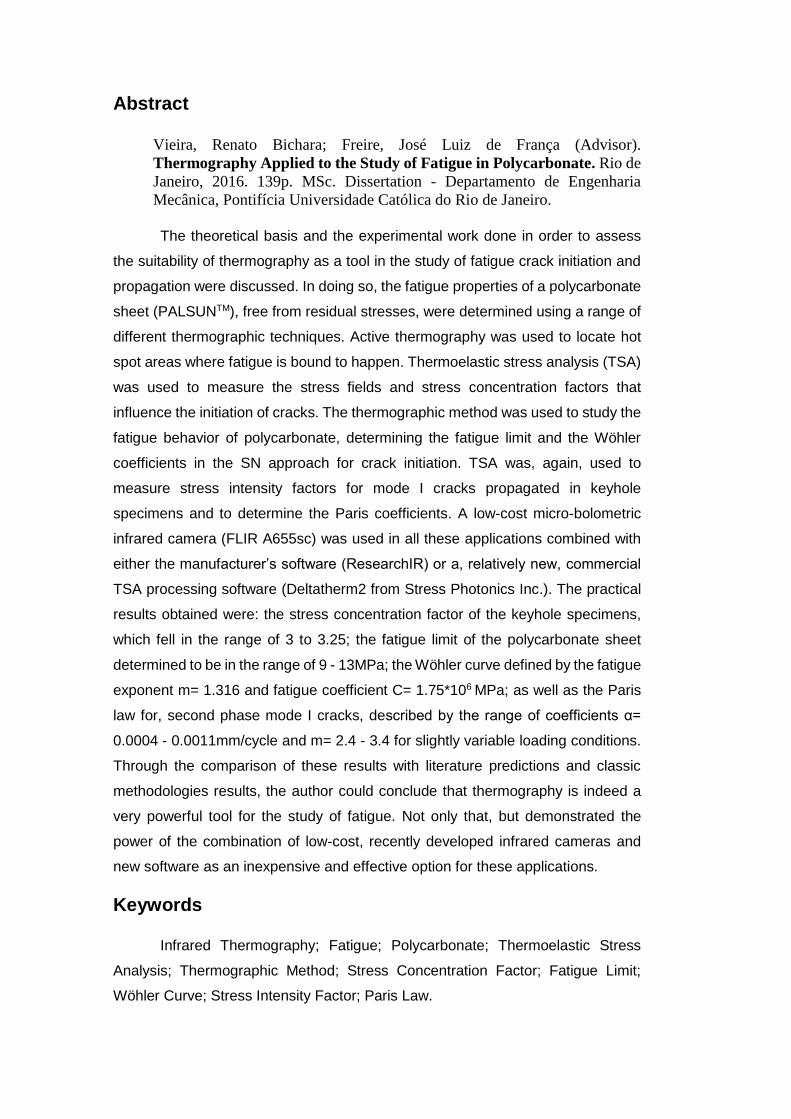
Vieira, Renato Bichara; Freire, José Luiz de França (Advisor).
Thermography Applied to the Study of Fatigue in Polycarbonate. Rio de
Janeiro, 2016. 139p. MSc. Dissertation - Departamento de Engenharia
Mecânica, Pontifícia Universidade Católica do Rio de Janeiro.
The theoretical basis and the experimental work done in order to assess
the suitability of thermography as a tool in the study of fatigue crack initiation and
propagation were discussed. In doing so, the fatigue properties of a polycarbonate
sheet (PALSUNTM), free from residual stresses, were determined using a range of
different thermographic techniques. Active thermography was used to locate hot
spot areas where fatigue is bound to happen. Thermoelastic stress analysis (TSA)
was used to measure the stress fields and stress concentration factors that
influence the initiation of cracks. The thermographic method was used to study the
fatigue behavior of polycarbonate, determining the fatigue limit and the Wöhler
coefficients in the SN approach for crack initiation. TSA was, again, used to
measure stress intensity factors for mode I cracks propagated in keyhole
specimens and to determine the Paris coefficients. A low-cost micro-bolometric
infrared camera (FLIR A655sc) was used in all these applications combined with
either the manufacturer’s software (ResearchIR) or a, relatively new, commercial
TSA processing software (Deltatherm2 from Stress Photonics Inc.). The practical
results obtained were: the stress concentration factor of the keyhole specimens,
which fell in the range of 3 to 3.25; the fatigue limit of the polycarbonate sheet
determined to be in the range of 9 - 13MPa; the Wöhler curve defined by the fatigue
exponent m= 1.316 and fatigue coefficient C= 1.75*106 MPa; as well as the Paris
law for, second phase mode I cracks, described by the range of coefficients α=
0.0004 - 0.0011mm/cycle and m= 2.4 - 3.4 for slightly variable loading conditions.
Through the comparison of these results with literature predictions and classic
methodologies results, the author could conclude that thermography is indeed a
very powerful tool for the study of fatigue. Not only that, but demonstrated the
power of the combination of low-cost, recently developed infrared cameras and
new software as an inexpensive and effective option for these applications.
Keywords
Infrared Thermography; Fatigue; Polycarbonate; Thermoelastic Stress
Analysis; Thermographic Method; Stress Concentration Factor; Fatigue Limit;
Wöhler Curve; Stress Intensity Factor; Paris Law.
DBD
PUC-Rio - Certificação Digital Nº 1412756/CA
Resumo
Vieira, Renato Bichara; Freire, José Luiz de França (Orientador).
Termografia Aplicada ao Estudo de Fadiga em Policarbonato. Rio de
Janeiro, 2016. 139p. Dissertação de Mestrado - Departamento de Engenharia
Mecânica, Pontifícia Universidade Católica do Rio de Janeiro.
As bases teóricas e o trabalho experimental desenvolvido na validação da
termografia como ferramenta de estudo de iniciação e propagação de trincas por
fadiga foram descritas. As propriedades de fadiga de uma placa de policarbonato
(PALSUNTM) isenta de tensões residuais foram determinadas usando-se
diferentes técnicas termográficas. A termografia ativa foi usada na localização de
pontos críticos onde o mecanismo de fadiga estará presente. A análise
termográfica de tensões (TSA) foi usada para medir os campos de tensão e fatores
de concentração de tensão que influenciam o surgimento de trincas. O método
termográfico foi usado na determinação do limite de fadiga e dos coeficientes da
curva de Wöhler no método SN de projeto contra iniciação de trincas. A TSA foi,
novamente, usada para determinação de fatores de intensidade de tensão e na
determinação dos coeficientes da lei de Paris. Em todos os experimentos, uma
câmera infravermelha micro bolométrica de baixo custo (FLIR A655sc) foi usada
em conjunto com o software da FLIR (ResearchIR) ou com um novo software
comercial de processamento de dados de TSA (Deltatherm2 da Stress Photonics
Inc.). Os resultados obtidos foram: o fator de concentração de tensão do espécime
tipo keyhole na faixa de 3 a 3.25; o limite de fadiga determinado na faixa 9 -13MPa;
a curva de Wöhler, definida pelo expoente de fadiga m= 1.316 e o coeficiente de
fadiga C= 1.75*106MPa; os coeficientes da lei de Paris para a fase 2 de trincas
propagadas em modo I, nas faixas α= 0.0004 - 0.0011mm/ciclo e m= 2.4 - 3.4 para
pequenas variações nas condições de carregamento. Com a comparação desses
resultados à literatura e com resultados obtidos mediante uso de métodos
clássicos, o autor pôde concluir que a termografia é uma técnica muito poderosa
no estudo de fadiga. Não só isso, mas demonstou a possibilidade do uso de novas
tecnologias, mais baratas, para câmeras infravermelhas de baixo custo em
combinação com novas soluções de software para realização desses estudos.
Palavras chaves
Termografia Infravermelha; Fadiga; Policarbonato; Análise Termoelástica
de Tensões; Método Termográfico; Fator de Concentração de Tensões; Limite de
Fadiga; Curva de Wöhler; Fator de Intensidade de Tensões; Lei de Paris.
DBD
PUC-Rio - Certificação Digital Nº 1412756/CA

Contents
1 Introduction 16
2 Thermography 19
2.1 Introduction 19
2.2 Infrared Thermography 20
2.2.1 Principles 20
2.2.2 Infrared Sensors 24
2.3 Active Thermography 26
2.4 Passive Thermography and Thermoelastic Stress Analysis (TSA) 26
2.4.1 Physics of TSA, the Thermoelastic Effect 27
2.4.2 Calibration and Practical Application of TSA 28
2.4.3 Data Acquisition and Interpretation 29
2.4.4 ‘DeltaTherm 2’ Software Peculiarities 30
2.4.5 Applications of TSA – Bibliographical Review 31
3 Brief Fatigue and Polycarbonate (PC) Review 32
3.1 Review of Basic Fatigue Concepts 32
3.1.1 Fatigue Crack Initiation and the Wohler curve 32
3.1.2 Stress Concentration 33
3.1.3 The Mean Stress Effect 34
3.1.4 Fatigue Crack Growth and Linear Elastic Fracture Mechanics 36
3.2 Polycarbonate Properties 40
3.2.1 Polycarbonate in Infrared Thermography 41
3.2.2 Polycarbonate in Fatigue Studies 41
4 Pre-Experimental Work 48
4.1 Introduction 48
4.2 The Specimens 48
4.2.1 Loading Cautions 49
4.2.2 Specimen Preparation 49
4.3 Cyclic Loading Machine 51
4.4 General Experimental Procedures and Cautions 52
4.4.1 Machine Cautions 52
4.4.2 Infrared Camera Cautions 53
5 Thermography Applied to Fatigue Crack Initiation 55
5.1 Locating Critical Points 55
5.2 Determining Stress Concentration Factors 56
DBD
PUC-Rio - Certificação Digital Nº 1412756/CA

5.2.1 Approach 1 – Simple Extrapolation of Line Data 56
5.2.2 Approach 2 – Stress Function and Principal Stresses Separation 61
5.3 Measuring Fatigue Limit Using Thermography 64
5.4 Determination of the Fatigue Curve Using Thermography 68
5.4.1 Φ Determination 70
5.4.2 SN curve determination 71
5.4.3 SN curve verification 74
6 Thermography Applied to Fatigue Crack Growth 76
6.1 Measuring Stress Intensity Factors Using TSA 76
6.1.1 The SIF Calculation Algorithm 76
6.1.2 Algorithm Inputs 77
6.1.3 Crack Tip Position Estimation and Point Coordinates Assignment 78
6.1.4 Model Validity Limits Verification 80
6.1.5 Error Function Construction and Minimization 81
6.1.6 SIF Calculation and Actual Crack Tip Location 83
6.2 Algorithm verification and Use 84
6.2.1 Numerically Generated TSA Data 84
6.2.2 SIF Measurements 85
6.3 Measuring the Crack Growth Rate 86
6.3.1 Crack Tip Accuracy of the Algorithm 86
6.3.2 da/dN Straight from Temperature Rise 88
6.4 Measuring da/dN vs ΔKI Curves 90
7 Final Considerations and Conclusions 96
7.1 Final Considerations 96
7.2 Conclusions 100
8 Bibliography 101
Appendix 1 Simple Test on Defect Location by Active Thermography 107
Appendix 2 Simple Test on Monitoring Cracks in Welded Joints 110
Appendix 3 PALSUNTM Polycarbonate Datasheet and Tensile Tests 113
Appendix 4 Measuring the Keyhole Kt with DIC and Photoelasticity 116
Appendix 5 Finite Elements Analysis of the Keyhole Specimen 121
Appendix 6 Photos of the Specimens 125
DBD
PUC-Rio - Certificação Digital Nº 1412756/CA
List of Figures
Figure 1.1: Diagram showing how thermography techniques
are divided. 16
Figure 1.2: Evolution of citations of Photoelasticity, TSA and
DIC found by google. 17
Figure 1.3: Summary of fatigue studies throughout this work. 17
Figure 2.1: My family as seen through a thermal camera. 19
Figure 2.2: Plot of Planck’s Law. 21
Figure 2.3: Atmosphere transmittance and atmospheric
windows [2]. 23
Figure 2.4: Cross section view of a microbolometer. 25
Figure 2.5: Camera FLIR A655sc, used in most of this work. 26
Figure 2.6: Typical TSA test procedure, adapted from [17]. 29
Figure 2.7: a) Magnitude and b) Phase maps of a TSA test
of a c) Notched aluminum plate, [17]. 30
Figure 2.8: Screenshot of the DeltaTherm 2 interface. 31
Figure 3.1: Typical SN curve, using Juvinall’s estimations for
steel (SR=1000MPa). 32
Figure 3.2: Concept of force lines. 33
Figure 3.3: Schematic Goodman’s curve. 35
Figure 3.4: Crack opening modes. 37
Figure 3.5: Schematic da/dN curve. 39
Figure 3.6: Paris law curves showing temperature effect,
adapted from [52]. 42
Figure 3.7: da/dN vs ΔK curves for three different thicknesses,
adapted from [54]. 43
Figure 3.8: Map of crack initiation mechanism, adapted from [58]. 45
Figure 3.9: SN curves for virgin and pre-stressed polycarbonate
specimens, adapted from [60]. 45
Figure 3.10: a) SN curve for polycarbonate specimens;
b) Damage Curve, adapted from [61]. 46
Figure 3.11: a) isothermal; b) non-isothermal fatigue curves for
polycarbonate, adapted from [62]. 46
Figure 3.12: Measured and predicted SN curves for polycarbonate,
adapted from [63]. 47
Figure 4.1: Dimensions of the constant radius specimens. 48
DBD
PUC-Rio - Certificação Digital Nº 1412756/CA
Figure 4.2: Dimensions of the Keyhole specimens. 49
Figure 4.3: Constant radius specimen mounted with custom grips. 49
Figure 4.4: a)Specimen before annealing. b)After annealing. 50
Figure 4.5: Photo of the pneumatic loading machine setup. 51
Figure 4.6: Screenshot of the program controlling the
pneumatic machine. 52
Figure 5.1: Cracked T-shaped specimen and critical points,
adapted from [17]. 55
Figure 5.2: a)TSA magnitude map and b)critical line plot for
CR specimen under Δσ=8.18MPa. 56
Figure 5.3: Calibration Stress vs TSA magnitude graph for
5 different Δσ. 57
Figure 5.4: a)TSA magnitude map; b)TSA phase map of a
keyhole specimen. 57
Figure 5.5: Magnitude line data for the keyhole specimen. 58
Figure 5.6: Phase line data for the keyhole specimen. 58
Figure 5.7: Magnitude data corrected by phase angle. 59
Figure 5.8: Treated TSA data points for keyhole specimen. 59
Figure 5.9: Normalized stress vs distance from notch plot
for keyhole. 60
Figure 5.10: Curve-fitted TSA data for keyhole specimen. 60
Figure 5.11: Area, in gray, for stress function fitting. 61
Figure 5.12: Fitted σθ field. 62
Figure 5.13: Fitted stress components for line ahead of notch. 63
Figure 5.14: TSA, DIC and Photoelasticity results for the line
ahead of notch. 64
Figure 5.15: T vs N curve for cyclic load above the fatigue limit,
adapted from [69]. 65
Figure 5.16: Loading steps for fatigue limit evaluation. 66
Figure 5.17: T(n) vs cycles points for 4 different load levels. 66
Figure 5.18: Thermographic image at the 7th load level. 67
Figure 5.19: T(N) vs σa eq for polycarbonate. 68
Figure 5.20: Illustration of the testing procedure for Risitano
method, adapted from [69]. 70
Figure 5.21: T(n) vs cycles graph for Φ measurement
(~25000cycles = approximately 1.5h test). 71
DBD
PUC-Rio - Certificação Digital Nº 1412756/CA
Figure 5.22: T(n) vs cycles graph of first specimen for SN curve
determination. 72
Figure 5.23: T(n) vs cycles graphs of second specimen for SN curve
determination. 73
Figure 5.24: SN curve measured via thermography. 74
Figure 5.25: SN curve with all data points. 74
Figure 6.1: Flowchart of the SIF calculation algorithm. 77
Figure 6.2: a)The magnitude map around a crack and
b)Typical y vs 1/S2 plot. 79
Figure 6.3: a)The phase map around a crack and
b)Typical phase vs x plot. 79
Figure 6.4: a)The radial direction where the curves are plotted
and b)Typical 1/S2 vs r plot 81
Figure 6.5: a)Illustration of Nelder-mead method for x ϵ R2. 82
Figure 6.6: a)Numerically generated TSA data for crack tip
at (-3,-1) and b)Calculated model for estimated crack tip at (-3,0). 84
Figure 6.7: Selected data points for SIF calculation of a 14.1mm
crack. 85
Figure 6.8: ΔKI/ΔP vs a plot for all experimental techniques
and FEM 86
Figure 6.9: Determined by TSA (red) and measured with photos
(green) cracks. 87
Figure 6.10: Position of 11 points along the crack path. 88
Figure 6.11: ΔT vs N plot for 11 points along crack path (left)
and integration areas for curves 3, 6 and 10 (rigth). 89
Figure 6.12: Comparison between ΔT/ΔP and da/dN. 90
Figure 6.13: da/dN (photos and TSA algorithm) vs ΔKI (TSA algorithm)
plot for first experiment. 91
Figure 6.14: da/dN (TSA algorithm) vs ΔKI (TSA algorithm and FEA)
plot for second experiment. 93
Figure 6.15: da/dN (temperature and photos) vs ΔKI (FEA)
plot for third experiment. 94
Figure 6.16: Plot of all da/dN results and references. 94
Figure A1.1: a)Composite and b)steel specimens for defect
detection experiment. 107
DBD
PUC-Rio - Certificação Digital Nº 1412756/CA

Figure A1.2: a)Thermographic image and b)Temperature profile for the
composite specimen. 108
Figure A1.3: a)Thermographic image and b)temporal plot of the
steel specimen. 109
Figure A2.1: Welded Joint, steel specimen. 110
Figure A2.2: Development of stresses on welded specimen’s surface. 110
Figure A2.3: Horizontal position of maximum stress region
throughout the cycles. 111
Figure A2.4: TSA vs cycles curves for the maximum stress points. 112
Figure A2.5: Damage for all points along the horizontal critical line. 112
Figure A3.1: PALSUN Datasheet. 113
Figure A3.2: Tensile specimen dimensions. 114
Figure A3.3: Stress vs displacement plots for a)CR and
b)Parallel tensile specimens. 114
Figure A3.4: Stress vs Strain curve for the tensile specimen. 115
Figure A4.1: Series of Photoelastic photos. 116
Figure A4.2: Normalized resulting photoelastic line data
ahead of the notch. 117
Figure A4.3: DIC pattern. 118
Figure A4.4: DIC principal strain field result. 119
Figure A4.5: DIC stress results ahead of the notch. 119
Figure A4.6: DIC fitted principal stress ahead of the notch. 120
Figure A5.1: Meshed symmetric model for FEA of the
keyhole specimen. 121
Figure A5.2: FEA resulting σy map for the keyhole specimen. 121
Figure A5.3: Kt vs thickness plot for the keyhole specimen. 122
Figure A5.4: Meshed model for SIF evaluation of the
keyhole specimen. 122
Figure A5.5: FEA resulting σy map for cracked (a=10mm)
keyhole specimen. 123
Figure A5.6: KI/P vs thickness plot for the cracked a=10mm)
keyhole specimen. 123
Figure A5.7: KI/P vs a plot for the keyhole specimen. 124
DBD
PUC-Rio - Certificação Digital Nº 1412756/CA

Figure A6.1: Fracture surface of CR tensile specimen
after tensile test. 126
Figure A6.2: Fracture surface of tensile specimen
after tensile test. 126
Figure A6.3: Fracture surface of CR tensile specimen
after fatigue testing. 127
Figure A6.4: Fracture surface of CR tensile specimen
after fatigue testing. 127
Figure A6.5: Fracture surface of CR tensile specimen
after fatigue bending testing. 128
Figure A6.6: Fracture surface of CR tensile specimen
after fatigue testing. 128
Figure A6.7: Fracture surface of Keyhole specimen
after fatigue testing Part 1. 129
Figure A6.8: Fracture surface of Keyhole specimen
after fatigue testing Part 2. 129
Figure A6.9: Fracture surface of Keyhole specimen
after fatigue testing Part 3. 130
Figure A6.10: Fracture surface of Keyhole specimen
after fatigue testing. 130
Figure A6.11: Fatigue crack propagated in a Keyhole specimen. 131
Figure A6.12: Fatigue crack propagated in a Keyhole specimen
(Tip detail). 131
Figure A6.13: Fatigue crack propagated in a Keyhole specimen. 132
Figure A6.14: Fatigue crack propagated in a Keyhole specimen
(Tip detail). 132
Figure A6.15: Fatigue crack propagated in a Keyhole specimen. 133
Figure A6.16: Fatigue crack propagated in a Keyhole specimen
(Tip detail). 133
Figure A6.17: Fatigue crack propagated in a Keyhole specimen. 134
Figure A6.18: Fatigue crack propagated in a Keyhole specimen
(Tip detail). 134
Figure A6.19: Fatigue crack propagated in a Keyhole specimen. 135
Figure A6.20: Fatigue crack propagated in a Keyhole specimen
(Tip detail). 135
DBD
PUC-Rio - Certificação Digital Nº 1412756/CA

Figure A6.21: Fretting damage and crack initiation in a
CR tensile specimen. 136
Figure A6.22: Fretting damage and crack initiation in a
CR tensile specimen. 136
Figure A6.23: Fretting crack in a CR tensile specimen (front view). 137
Figure A6.24: Fretting crack in a CR tensile specimen (oblique view). 137
Figure A6.25: Fretting fracture surface. 138
Figure A6.26: Fretting fracture surface (zoom). 138
Figure A6.27: Fretting fracture surface (initiation detail). 139
DBD
PUC-Rio - Certificação Digital Nº 1412756/CA

List of Tables
Table 2.1: Emissivity of some materials and paints. 23
Table 3.1: Average vaues of some polycarbonate properties. 40
Table 3.2: Reported values of Paris coefficients at various
temperatures, adapted from [52]. 42
Table 3.3: Paris coefficients reported for different
stress ratios and thicknesses, adapted from [55]. 44
Table 4.1: Temperatures and times of the adapted annealing
heat treatment. 50
Table 5.1: Results for the Kt of the keyhole specimen. 64
Table 5.2: Summarized results for the fatigue limit test. 67
Table 5.3: Results of first specimen for SN curve determination. 72
Table 5.4: Results of second specimen for SN curve determination. 73
Table 6.1: Results for the SIF measurement using TSA,
DIC and FEM. 85
Table 6.2: Results for crack tip position and crack length. 87
Table 6.3: Damage parameter result for 11 points along crack path. 89
Table 6.4: Results for the first crack propagation da/dN test. 91
Table 6.5: Results for the second crack propagation da/dN test. 92
Table 6.6: Results for the third crack propagation da/dN test. 93
Table A4.1: Fringe distance from notch tip. 116
DBD
PUC-Rio - Certificação Digital Nº 1412756/CA
16
1
Introduction
Thermography is a research field, which consists in using infrared radiation
in order to measure the temperature map of a surface using infrared radiation.
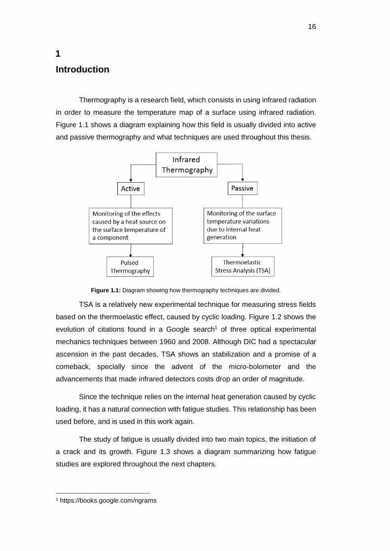
Figure 1.1 shows a diagram explaining how this field is usually divided into active
and passive thermography and what techniques are used throughout this thesis.
Figure 1.1: Diagram showing how thermography techniques are divided.
TSA is a relatively new experimental technique for measuring stress fields
based on the thermoelastic effect, caused by cyclic loading. Figure 1.2 shows the
evolution of citations found in a Google search1 of three optical experimental
mechanics techniques between 1960 and 2008. Although DIC had a spectacular
ascension in the past decades, TSA shows an stabilization and a promise of a
comeback, specially since the advent of the micro-bolometer and the
advancements that made infrared detectors costs drop an order of magnitude.
Since the technique relies on the internal heat generation caused by cyclic
loading, it has a natural connection with fatigue studies. This relationship has been
used before, and is used in this work again.
The study of fatigue is usually divided into two main topics, the initiation of
a crack and its growth. Figure 1.3 shows a diagram summarizing how fatigue
studies are explored throughout the next chapters.
1 https://books.google.com/ngrams
DBD
PUC-Rio - Certificação Digital Nº 1412756/CA

17
Figure 1.2: Evolution of citations of Photoelasticity, TSA and DIC found by google.
Figure 1.3: Summary of fatigue studies throughout this work.
The main objective of this work can be simply put as the assessment of the
suitability of thermography, and the use of an inexpensive equipment combined
with a new processing software, for the study of the fatigue behavior of
polycarbonate. In order to accomplish that, a series of experiments was conducted
and divided into 6 chapters and 5 appendixes summarized below.
Chapter 2 presents a review of thermography theory and experimental
applications, from active to passive thermography passing through the workings of
typical detectors and specifics of the equipment used in the tests described later.
Chapter 3 briefly reviews simple fatigue concepts and presents a
bibliographical review of the results found for polycarbonate. The importance of
this material and its fatigue properties are discussed as well.
DBD
PUC-Rio - Certificação Digital Nº 1412756/CA

18
Chapter 4 summarizes the experimental procedures and cautions related
to the load-testing machine and to the infrared camera used in this investigation. It
also shows the specimens used and the preparations needed.
Chapter 5 starts reporting the experimental phase of the work, discussing
the use of thermography for the study of fatigue crack initiation. From hotspot
detection all the way to acquiring SN data and fatigue properties of the material,
such as the fatigue limit.
Chapter 6 continues reporting the experimental work, stepping into the
fatigue crack growth study. It presents the development of an algorithm for stress
intensity range measurement as well as the application of thermography in
measuring crack growth fatigue curves for polycarbonate.
Finally, Chapter 7 summarizes all the conclusions made throughout the
previous chapters and evaluates the suitability of the procedures used in the study
of the fatigue behavior of polycarbonate.
Six Appendixes are located at the end of the text, showing experiments on
defect location, crack growth monitoring, material characterization of the
polycarbonate sheet, measurement of stress concentration factors using digital
image correlation (DIC) and photoelasticity, finite elements analysis of the
specimen used for fatigue crack propagation studies and the final appendix
showing photos of all specimens (fractured and not-fractured).
DBD
PUC-Rio - Certificação Digital Nº 1412756/CA

19
2
Thermography
2.1
Introduction
Thermography is a specific area of study within the large field of
temperature measurements. It consists of using thermal cameras in order to
measure the temperature distribution of an object’s surface. In general, it can be
split into two different types of experiments, active and passive thermography,
which will be explained in further subchapters.
The images generated in thermography, usually called thermograms, use
pseudo-color techniques to display the temperature variations. This way, a color is
attributed to each temperature level, continuously or discretely, making it much
easier for humans to notice the intensity variations. Figure 2.1 was taken at the
Deutsche Museum in Munich, and shows my family. It is easy to see the areas
where the temperature is higher, because of the colors assigned.
Figure 2.1: My family as seen through a thermal camera.
In order to know the exact values, in degrees, a scale is required to correlate each
one of the colors to a specific temperature level. In the picture above, the scale is
missing.
DBD
PUC-Rio - Certificação Digital Nº 1412756/CA

20
The most common type of thermal camera uses infrared radiation levels to
infer the temperature of a surface. Because of that, this work focuses on the use
of infrared thermography.
2.2
Infrared Thermography
William Herschel’s first observations of the infrared (IR) spectrum, in 1800,
measured the “power” of the heat radiation of the below-red wavelengths of the
electromagnetic spectrum. He concluded that the invisible portion of light carried
more “power” than the visible. Because of that, infrared radiation became the most
common and efficient way of measuring temperature in no-contact applications [1].
2.2.1
Principles
Any object with temperature above 0K will emit radiation. For temperatures
below 773K, this radiation will lie completely within the IR wavelengths (900 –
14000nm). In addition to emitting radiation, a body will react to it in three different
ways, depending on its properties. It will absorb, reflect and transmit portions of
the radiation. This behavior originates the Total Radiation Law, which can be
written as: [2]
𝟏 = 𝛼 + 𝜌 + 𝜏 ( 2.1 )
where α, ρ and τ are the coefficients that describe the object’s incident energy
absorption, reflection and transmission respectively.
Each object will have a different set of coefficients depending on it’s
properties, for example, a perfect blackbody would have ρ=τ=0 and α=1, since, by
definition, it absorbs all the incident radiation.
The concept of a blackbody, that is a perfect absorber and emitter of radiant
energy, comes from Kirchhoff’ s Law of thermal radiation, which states that the
emissivity (ε) of a body is equal to its absorptivity (α):
𝛼 = 휀 ( 2.2 )
Using equation 2.2 into equation 2.1, and assuming a perfect blackbody
(τ=ρ=0), we have:
휀𝑏𝑏 = 1 ( 2.3 )
where the subscript bb indicates a blackbody. From this, the concept of emissivity
for an object that is not a perfect blackbody can be written:
DBD
PUC-Rio - Certificação Digital Nº 1412756/CA

21
휀 =𝛷𝑜𝑏𝑗
𝛷𝑏𝑏⁄
( 2.4 )
where, Φobj and Φbb are the total radiant energy emitted by a real object and by a
blackbody at the same temperature, respectively.
Planck’s Law describes the energy radiated by a blackbody as a function
of its temperature and of the wavelength of emission.
𝛷𝑏𝑏(𝜆, 𝑇) =𝐶1
𝜆5(exp(𝐶2
𝜆𝑇⁄ ) − 1)
( 2.5 )
with,
𝐶1 = 2𝜋𝑐2ℎ ( 2.6 )
𝐶2 =𝑐ℎ
𝑘
( 2.7 )
where, C1 is the first constant of radiation, C2 is the second constant of radiation, λ
is the wavelength of the emission, T is the temperature of the blackbody, c is the
speed of light in the medium, h is the Planck’s constant (~6.626 × 10⁻³⁴ m2 kg s-1)
and k is the Boltzmann constant (~1.381 × 10⁻²³ m2 kg s-2 K-1).
Figure 2.2, below, shows the plot of Plank’s Law for various temperature
levels:
Figure 2.2: Plot of Planck’s Law.
1000ºC
800ºC
600ºC
400ºC
200ºC
DBD
PUC-Rio - Certificação Digital Nº 1412756/CA
22
Integrating the Plank’s law, the result describes the total energy radiated by
a blackbody as a function of its temperature:
𝛷𝑏𝑏 = ∫𝛷𝑏𝑏(𝜆, 𝑇)
𝜆
= 𝐵𝑇4 ( 2.8 )
where, B is the Stefan-Boltzmann constant (5.670 × 10⁻⁸ W m−2 K−4) and T is the
blackbody’s temperature.
Using equations 2.4 and 2.8 it is easy to determine the total energy emitted
by an object:
𝛷𝑜𝑏𝑗 = 휀𝐵𝑇4 ( 2.9 )
where 0< ε <1 is the object’s emissivity.
In reality, emissivity is a function of the wavelength of emission ε(λ).
Because of that, equation 2.9 actually describes the total energy radiated by a
theoretical object, called grey-body.
The definition of a grey-body is a body that emits radiation in constant
proportion to the corresponding blackbody. For reasons still to be discussed,
infrared thermography uses only small windows of wavelength to measure
temperature, and because of that, the approximation of real life objects as grey-
bodies is acceptable [2].
Between the surface which the temperature is being measured and the
infrared sensor usually is the atmosphere. Earth’s atmosphere itself interacts with
radiation like any other object. It can absorb, transmit and reflect the energy.
Because of that, the total radiation that reaches the sensor is the sum of three
portions:
𝛷𝑠𝑒𝑛𝑠𝑜𝑟 = 𝜏𝑎𝑡𝑚𝛷𝑜𝑏𝑗 +𝜌𝑜𝑏𝑗𝜏𝑎𝑡𝑚𝛷𝑎𝑚𝑏 +휀𝑎𝑡𝑚𝛷𝑎𝑡𝑚 ( 2.10 )
(1) (2) (3)
where:
(1) The energy radiated by the object Φobj after being attenuated by the
atmosphere’s transmittance τatm.
(2) The energy radiated by the ambient Φamb after being reflected by the object
ρobj and then attenuated by the atmosphere’s transmittance τatm.
(3) The energy radiated by the atmosphere itself.
DBD
PUC-Rio - Certificação Digital Nº 1412756/CA
23
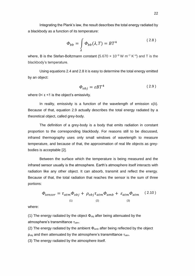
Assuming that the object is opaque to infrared wavelength (τobj=0) and that
the atmosphere does not reflect radiation (ρatm=0), equation 2.10 is rewritten, by
using the Total Radiation Law (Equation 2.1):
𝛷𝑠𝑒𝑛𝑠𝑜𝑟 = 𝜏𝑎𝑡𝑚𝛷𝑜𝑏𝑗 + (1 − 휀𝑜𝑏𝑗)𝜏𝑎𝑡𝑚𝛷𝑎𝑚𝑏 + (1 − 𝜏𝑎𝑡𝑚)𝛷𝑎𝑡𝑚 ( 2.11 )
(1) (2) (3)
The conclusions from equation 2.11 are that maximizing the atmosphere’s
transmittance and the object’s emissivity are the key to amplifying the portion of
the energy that reaches the sensor that is radiated by the object, while reducing
the noise. In order to do that, infrared sensors use so-called “atmospheric
windows”, specific wavelength intervals that are almost not absorbed by Earth’s
atmosphere. Figure 2.3 shows the infrared atmospheric transmittance and the two
typical “windows” used by commercial sensors (3-5μm and 8-14μm):
Figure 2.3: Atmosphere transmittance and atmospheric windows [2].
Table 2.1 shows the emissivity of typical material and paints that are
typically used to maximize the surface’s emissivity:
Aluminum Polished 0.04-0.05
Oxidized 0.10-0.31
Anodized 0.55-0.72
Steel Polished 0.07-0.09
Oxidized 0.79
Paint Matt Black lacquer 0.97
White enamel 0.92
oil 0.89-0.97
PVC 0.91-0.93
Insulating Tape Black 0.97
Table 2.1: Emissivity of some materials and paints.
DBD
PUC-Rio - Certificação Digital Nº 1412756/CA

24
2.2.2
Infrared Sensors
Infrared sensors can be divided into two categories: Cooled detectors and
Uncooled detectors. Both have advantages and disadvantages that are discussed
below [2]:
Cooled detectors
Also known as quantum or photon detectors, this kind of infrared sensor
uses the same principle of most common digital cameras, the only difference being
the constituent materials. Basically, when a photon of a specific wavelength range
hits the semiconductor it is absorbed, causing an electron of an atom to jump to a
higher energy state. What is then measured is the change in conductivity caused
by this phenomenon.
Because of how they work, and the high sensitivity of the process, the
quantum detectors must be cooled to very low temperatures, typically around the
60-100K range. This need causes these sensors to be very expensive not only to
produce but to operate as well, since the cooling process in very energy-intensive
and time-consuming.
Although much more expensive, the photon detectors have higher
sensitivity and accuracy, because of that, they can achieve much higher resolution
cameras. Another advantage is the possibility of using both atmospheric windows
(3-5 and 8-14μm), depending on the constitution and construction of the sensor.
Until recently, photon detectors were the only viable choice for practical
thermography applications. Reference [3] presents a comprehensive guide to
photon detectors.
Uncooled detectors
This kind of sensor works based on a simpler principle. It absorbs the
infrared radiation causing its temperature to rise, this rise in temperature then
causes a change in an electrical property, such as resistance, which is then read
by a proper circuit. Because of how it works, it is sometimes called thermal
detector.
Exactly because it depends on a change in its temperature, the thermal
detector does not need to be cooled down. Because of that, its cost is an order of
magnitude lower than the cooled ones, both to produce and to operate.
DBD
PUC-Rio - Certificação Digital Nº 1412756/CA
25
The main disadvantages of the uncooled detectors are the lower sensitivity
and the restriction to the higher wavelength atmospheric window (8-14μm). It was
not until recent advancements that these sensors became viable for practical
thermography.
The American astronomer Samuel Pierpont Langley discovered, in 1878,
the main type of thermal detector, the bolometer [4]. By the late 70’s,
microbolometers were developed by Honeywell for the US Department of Defense,
being declassified in 1992 when a series of manufacturers started producing and
developing cameras with microbolometer arrays. From then on, thermal detectors
would start to see more use in scientific applications [5].
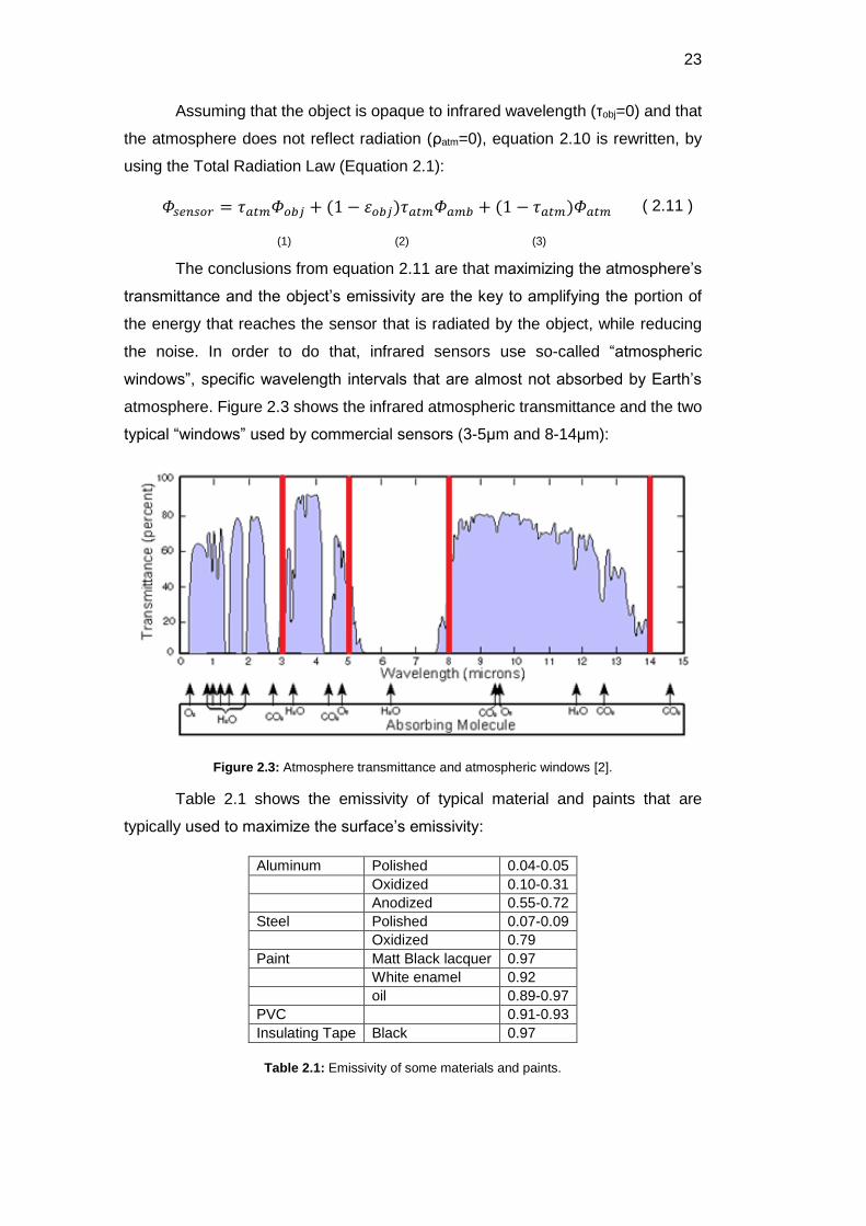
Figure 2.4 shows a scheme of a microbolometer making it easier to
understand how it works.
Figure 2.4: Cross section view of a microbolometer.
Because of the principle on which the bolometer is based, it has an intrinsic
disadvantage. When compared to cooled detectors, they present a rather slow
thermal time constant, proportional to the time required for the mass of the
absorber to reach a stable temperature. This time is reported to be of the order of
40-50ms, which results in a maximum frame rate of about 25Hz. For applications
where the temperature transient is much faster than this, quantum detectors must
be used to read accurate temperature values [6].
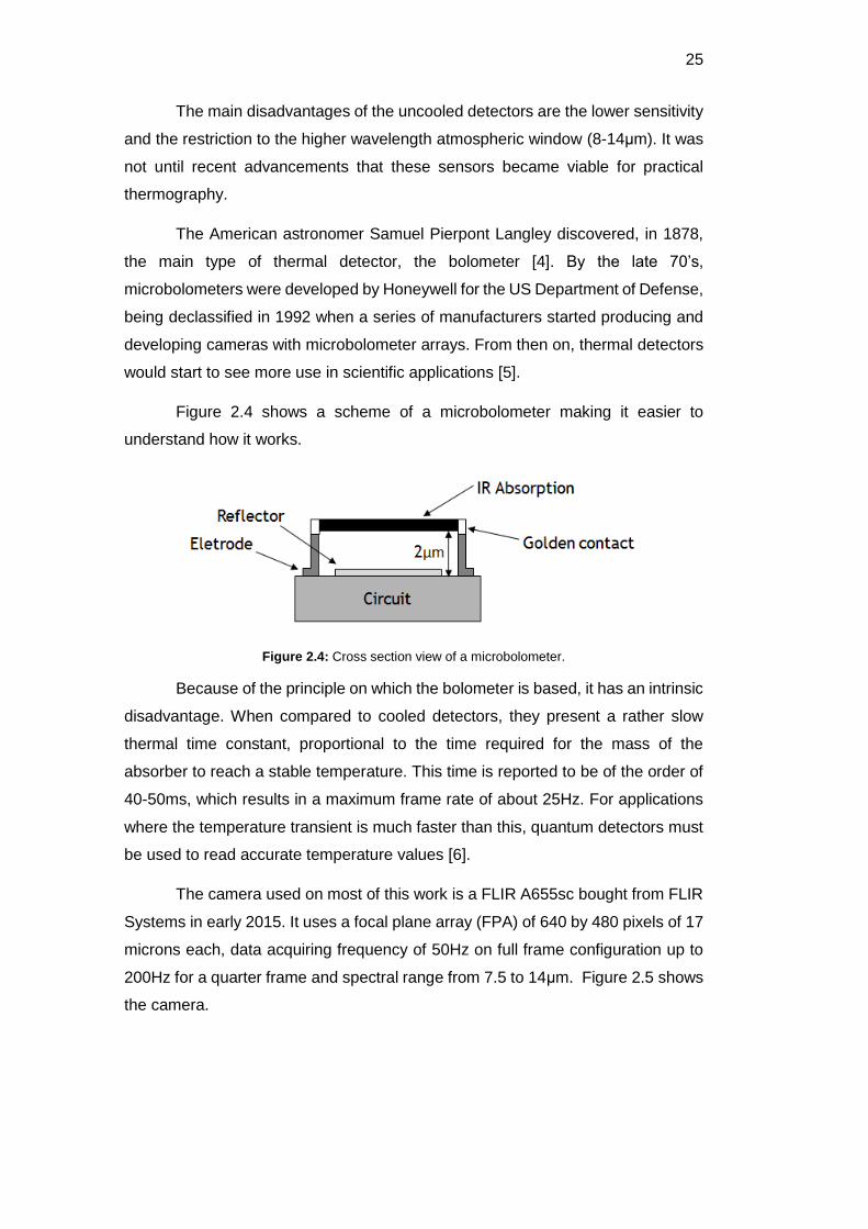
The camera used on most of this work is a FLIR A655sc bought from FLIR
Systems in early 2015. It uses a focal plane array (FPA) of 640 by 480 pixels of 17
microns each, data acquiring frequency of 50Hz on full frame configuration up to
200Hz for a quarter frame and spectral range from 7.5 to 14μm. Figure 2.5 shows
the camera.
DBD
PUC-Rio - Certificação Digital Nº 1412756/CA

26
Figure 2.5: Camera FLIR A655sc, used in most of this work.
It can switch between two different temperature ranges (-40 – 150ºC and
100 – 650ºC) with a <30mK sensitivity in both of them.
2.3
Active Thermography
Active thermography consists of measuring the effects of a heat source on
an object. Usually measuring differences on the rates of heating or decaying, it can
be used to detect features that do not generate heat by themselves. One use,
outside the engineering research field, are the active night-vision goggles, that
combine infrared illuminators with detectors and make it possible to see a
monochromatic view of a low light ambient.
In mechanical engineering, the most common use of active thermography
is the detection of defects in structures. Ibarra-Castanedo [7], presents a great
discussion about this use of thermography, emphasizing the use of pulsed
thermography. This technique, as well as pulsed-phase and lock-in thermography,
have been used many times to locate defects and predict their sizes and depths
[7]-[11].
Appendix 1 describes a simple test on defect location using pulsed
thermography that was developed during the experimental phase of the present
work.
2.4
Passive Thermography and Thermoelastic Stress Analysis (TSA)
While active thermography requires a heat source, passive thermography,
as the name suggests, does not. It relies on temperature variations already existent
in the analyzed object, usually caused by heat generation within it.
DBD
PUC-Rio - Certificação Digital Nº 1412756/CA

27
Passive thermography has many applications in various fields of study.
Some examples are: Passive night-vision, for defense and surveillance, for
electronic components monitoring and for medical examinations [12]. A very recent
application that was employed in many airports worldwide was to examine
passengers for fever during the 2009 swine flu (H1N1 Influenza) pandemic.
In the experimental mechanics field, maybe the most used passive
thermography technique, and main focus of the present work, is the so-called
Thermoelastic Stress Analysis (TSA) technique.
2.4.1
Physics of TSA, the Thermoelastic Effect
Towards the end of the 19th century, William Thomson (Lord Kelvin)
documented the thermoelastic effect for the first time [13].
He discovered that when a solid materials is subjected to tensile stress its
temperature rises slightly and when a compressive stress is applied, the
temperature drops in the same proportion.
In reality, the change in temperature caused by the thermoelastic effect is
proportional to the sum of the principal stresses acting in the body. The following
equation describes this phenomenon:
𝛥𝑇 =−𝛼𝑇𝑜𝜌𝑐𝑝
(∆𝜎1 + ∆𝜎2) ( 2.12 )
where, α is the linear thermal expansion coefficient, T0 is a reference temperature,
ρ is the density of the material, cp is the specific heat at constant pressure and σ1
and σ2 are the principal stresses.
A simplified deduction of equation 2.12 is shown herein, while the complete
thermodynamics arguments for it can be found in the literature [14].
A small change in temperature in a body depends on its stress state, the
strains that are being applied and the heat exchange profile (conduction) within the
solid [15].
�̇� =𝑇0𝜌𝐶𝜀
∂𝜎𝑖𝑗∂T
휀�̇�𝑗 +�̇�
𝜌𝐶𝜀
( 2.13 )
where, T0 is a reference temperature, ρ is the density of the material, Cε is the
specific heat at constant strain, σij is the stress tensor, ε̇ij is the rate of change in
the strain tensor and Q̇ is the rate of heat production per unit volume.
DBD
PUC-Rio - Certificação Digital Nº 1412756/CA

28
In TSA, the standard approach is to apply a cyclic load to the specimen at
a frequency in which no heat conduction takes place, making it possible to neglect
the second term of equation 2.13. Because of that, it is safe to say that the sensor
will only be measuring the surface temperature variation, and the stress-strain-
temperature relationship for an isotropic material in plane stress conditions have
to be used.
𝜎𝑖𝑗 = 2𝜇휀𝑖𝑗 +(𝜆휀𝑘𝑘 − 𝛽𝛿𝑇)𝛿𝑖𝑗 ( 2.14 )
where δij is the Kronecker delta and
𝜇 =𝐸
2(1 + 𝜈)𝜆 =
𝜈𝐸
(1 + 𝜈)(1 − 2𝜈)𝛽 = (3𝜆 + 2𝜇)𝛼
( 2.15 )
where, ν is the Poisson’s coefficient, E is the Young’s modulus and α is the linear
thermal expansion coefficient.
Deriving equation 2.14 with respect to T, and assuming that the linear
constants do not vary with temperature:
∂𝜎𝑖𝑗∂T
= −𝛽𝛿𝑖𝑗 ( 2.16 )
Then, substituting equation 2.16 into equation 2.13:
�̇� = −𝑇0𝛽
𝜌𝐶𝜀휀�̇�𝑘
( 2.17 )
Using equations 2.14 and 2.15:
�̇� = −𝛼 [𝑇0𝜌𝐶𝜀
+1 − 2𝜈
3𝛼2𝐸] �̇�𝑘𝑘
( 2.18 )
Knowing that Cε can be written as a function of Cp:
𝐶𝜀 = 𝐶𝑃 −3𝐸𝛼𝑇0
𝜌(1 − 2𝜈)
( 2.19 )
Plugging equation 2.19 into equation 2.18 and integrating it, the result is
equation 2.12.
2.4.2
Calibration and Practical Application of TSA
As discussed before, for the application of TSA, infrared cameras,
governed by equation 2.9, are used. Deriving equation 2.9:
DBD
PUC-Rio - Certificação Digital Nº 1412756/CA

29
𝛥𝛷𝑜𝑏𝑗 = 4휀𝐵𝑇3𝛥𝑇 ( 2.20 )
Plugging equation 2.19 into equation 2.20 and rearranging it results in:
∆𝜎1 + ∆𝜎2 = −𝛥𝛷𝑜𝑏𝑗
4휀𝐵𝑇3𝜌𝑐𝑝𝛼𝑇𝑜
( 2.21 )
Considering the response S from the detector as being proportional to ΔΦobj
by a gain Z (property of the sensor):
𝑆 =−4𝑍휀𝐵𝑇3𝛼𝑇𝑜
𝜌𝑐𝑝(∆𝜎1 + ∆𝜎2)
( 2.22 )
Finally, in practical uses of the TSA technique, measuring all the material
and sensor properties is not needed. The typical application uses a simple
calibration process that consists of using an object with a known stress state (Δσ1
+ Δσ2), like a simple tensile specimen, to determine a coefficient A that is used as
described [16]:
𝐴𝑆 = (∆𝜎1 + ∆𝜎2) ( 2.23 )
2.4.3
Data Acquisition and Interpretation
As stated before, typical TSA applications require a cyclic loading, and by
combining the thermographic signal and the load signal in what is called a lock-in
process, the magnitude and signal of the first invariant of the stress tensor can be
determined [15]. Figure 2.6 shows, schematically, a typical TSA test.
Figure 2.6: Typical TSA test procedure, adapted from [17].
From the infrared camera signal and through equation 2.23, the magnitude
of the stress invariant is determined. By correlating both signals, the phase map is
DBD
PUC-Rio - Certificação Digital Nº 1412756/CA
30
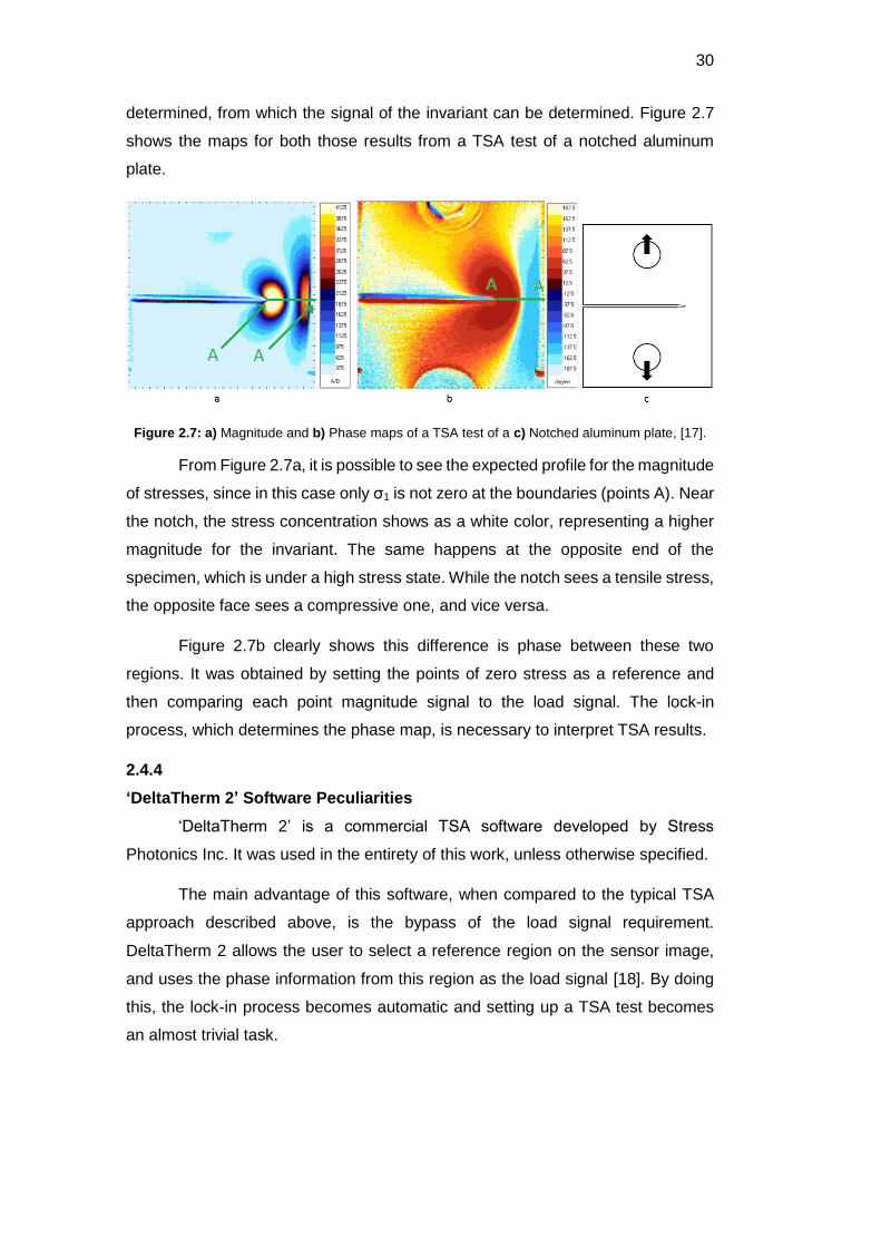
determined, from which the signal of the invariant can be determined. Figure 2.7
shows the maps for both those results from a TSA test of a notched aluminum
plate.
Figure 2.7: a) Magnitude and b) Phase maps of a TSA test of a c) Notched aluminum plate, [17].
From Figure 2.7a, it is possible to see the expected profile for the magnitude
of stresses, since in this case only σ1 is not zero at the boundaries (points A). Near
the notch, the stress concentration shows as a white color, representing a higher
magnitude for the invariant. The same happens at the opposite end of the
specimen, which is under a high stress state. While the notch sees a tensile stress,
the opposite face sees a compressive one, and vice versa.
Figure 2.7b clearly shows this difference is phase between these two
regions. It was obtained by setting the points of zero stress as a reference and
then comparing each point magnitude signal to the load signal. The lock-in
process, which determines the phase map, is necessary to interpret TSA results.
2.4.4
‘DeltaTherm 2’ Software Peculiarities
‘DeltaTherm 2’ is a commercial TSA software developed by Stress
Photonics Inc. It was used in the entirety of this work, unless otherwise specified.
The main advantage of this software, when compared to the typical TSA
approach described above, is the bypass of the load signal requirement.
DeltaTherm 2 allows the user to select a reference region on the sensor image,
and uses the phase information from this region as the load signal [18]. By doing
this, the lock-in process becomes automatic and setting up a TSA test becomes
an almost trivial task.
DBD
PUC-Rio - Certificação Digital Nº 1412756/CA
31
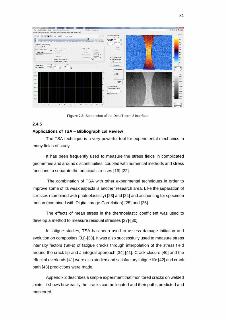
Figure 2.8: Screenshot of the DeltaTherm 2 interface.
2.4.5
Applications of TSA – Bibliographical Review
The TSA technique is a very powerful tool for experimental mechanics in
many fields of study.
It has been frequently used to measure the stress fields in complicated
geometries and around discontinuities, coupled with numerical methods and stress
functions to separate the principal stresses [19]-[22].
The combination of TSA with other experimental techniques in order to
improve some of its weak aspects is another research area. Like the separation of
stresses (combined with photoelasticity) [23] and [24] and accounting for specimen
motion (combined with Digital Image Correlation) [25] and [26].
The effects of mean stress in the thermoelastic coefficient was used to
develop a method to measure residual stresses [27]-[30].
In fatigue studies, TSA has been used to assess damage initiation and
evolution on composites [31]-[33]. It was also successfully used to measure stress
intensity factors (SIFs) of fatigue cracks through interpolation of the stress field
around the crack tip and J-integral approach [34]-[41]. Crack closure [40] and the
effect of overloads [41] were also studied and satisfactory fatigue life [42] and crack
path [43] predictions were made.
Appendix 2 describes a simple experiment that monitored cracks on welded
joints. It shows how easily the cracks can be located and their paths predicted and
monitored.
DBD
PUC-Rio - Certificação Digital Nº 1412756/CA

32
3
Brief Fatigue and Polycarbonate (PC) Review
3.1
Review of Basic Fatigue Concepts
The study of fatigue is usually divided in two main fields. Crack initiation and
crack growth. Basic concepts of both fields, which are used throughout this work,
are reviewed in this section.
3.1.1
Fatigue Crack Initiation and the Wohler curve
The most used approach for fatigue dimensioning is the so-called Wöhler
method (or SN method). Simply put, this approach uses the correlation between
the amplitude of the cyclic stresses acting at a critical point and the number of
loading cycles necessary for a fatigue crack to initiate. The SN curve (Wöhler
curve) is the plot of this correlation, and can be used to predict the number of cycles
a specimen at a given alternate stress level can sustain before failing. The most
common equation used to adjust data in the Wöhler curve is the parabolic
relationship that linearizes the data in a log-log plot [44].
𝑁𝑆𝑚 = 𝐶 ( 3.1 )
where N is the number of cycles until failure, S is the stress amplitude (S=σa=Δσ/2),
m and C are material constants known as fatigue exponent and fatigue coefficient,
respectively. Figure 3.1 shows a typical SN curve, using Juvinall’s estimations for
a carbon steel with ultimate strength of 1000MPa in rotating bending test [44].
Figure 3.1: Typical SN curve, using Juvinall’s estimations for steel (SR=1000MPa).
DBD
PUC-Rio - Certificação Digital Nº 1412756/CA
33
In practice, although very useful, approximations like the ones made by
Juvinall [44] can produce non-conservative predictions. Because of that, measured
SN curves are very important, as they are capable of characterizing the fatigue
behavior of a specific material.
Each point of the curve represents one specimen that was cyclic loaded
until failure, and very high number of cycles are needed for the lower stress points.
In addition, because fatigue is a naturally statistical problem, the data usually
presents high dispersion, especially for the lower stress points. It is easy to see
why measuring SN curves is very time consuming. There are some proposed
methods to accelerate this process. One of these, called the Risitano method,
which uses thermography to determine the Wöhler curve, is used to measure the
SN curve of polycarbonate further on.
From what has been said about the SN method, it is clear that stress
analysis plays a huge role in this approach, since it is very important to know the
actual stresses acting at the critical point of a component in order to determine it’s
fatigue life even when having access to a measured SN curve. Two aspects of
stress analysis, that are going to be used in later chapters, are discussed next.
3.1.2
Stress Concentration
Geometrical discontinuities usually cause a phenomenon called stress
concentration. The concept of force lines is very useful in understanding why that
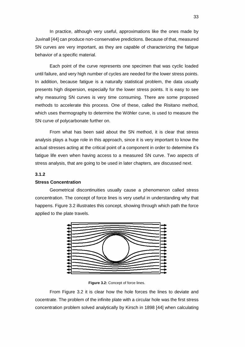
happens. Figure 3.2 illustrates this concept, showing through which path the force
applied to the plate travels.
Figure 3.2: Concept of force lines.
From Figure 3.2 it is clear how the hole forces the lines to deviate and
cocentrate. The problem of the infinite plate with a circular hole was the first stress
concentration problem solved analytically by Kirsch in 1898 [44] when calculating
DBD
PUC-Rio - Certificação Digital Nº 1412756/CA

34
the circumferential stresses around the hole boundary. He arrived at the following
expression.
𝜎𝜃(𝑟, 𝜃) =𝜎𝑛2[(1 +
𝑅2
𝑟2) − (1 +
3𝑅4
𝑟4) 𝑐𝑜𝑠2𝜃]
( 3.2 )
where, σθ(r,θ) is the circumferential stress as a function of r (the distance from the
center of the hole) and θ (the angle with the direction of the stress applied to the
plate), σn is the nominal stress applied to the plate and R is the radius of the hole.
When r=R and θ=±π/2, the circumferential stress assumes its maximum
value. σmax= 3σn. The concept of stress concentration factor (Kt) is defined as.
𝐾𝑡 =𝜎𝑚𝑎𝑥
𝜎𝑛= 3(𝑓𝑜𝑟𝐾𝑖𝑟𝑠𝑐ℎ′𝑠𝑝𝑟𝑜𝑏𝑙𝑒𝑚)
( 3.3 )
The implications of this phenomenon are that even if the hole will not
change the nominal stresses applied to the plate, the real stress acting at the
critical point of the component is 3 times higher. Stress concentration regions, the
so-called hot spots, are where fatigue cracks initiate and cause fatigue failure.
Thermoelasticity is a very powerful tool in measuring stress concentrations,
since it provides a full-field stress map of the specimen surface, and because
stress concentrations usually happens at free surfaces, one of the principal
stresses is always zero, making the TSA data a direct measurement of the
maximum circumferential stress. TSA, in conjunction with photoelasticity and
Digital Image Correlation techniques, was used to measure stress concentration
factors of aluminum u-notch and polycarbonate keyhole specimens by the author
in [45] and [46].
3.1.3
The Mean Stress Effect
Generally, two driving forces, maximum stress and stress range, govern
fatigue effects. The usual way to consider both when predicting the fatigue life of a
component is to use a constant life diagram to determine the equivalent completely
alternating stress, that would result in the same life as the real stress acting on the
specimen [44].
The most used model of a constant life diagram is the Goodman’s rule. It
linearly correlates the alternating stress (σa) and the mean stress (σm) with the
following equation.
DBD
PUC-Rio - Certificação Digital Nº 1412756/CA

35
𝜎𝑎𝑆𝐹(𝑁)
+𝜎𝑚𝑆𝑅
= 1 ( 3.4 )
where SF(N) is the fatigue strength for a specific number of cycles and SR is the
ultimate tensile strength.
If SF is taken at a number of cycles high enough to be considered infinite
life, SF will be the fatigue limit of the material, and the Goodman curve plotted in
Figure 3.3 determines the points which will eventually fail (above the curve) and
the point which will not (below the curve).
Figure 3.3: Schematic Goodman’s curve.
Rearranging Equation 3.5 the equivalent alternating stress (σa-eq) is
determined as:
𝜎𝑎−𝑒𝑞 =𝜎𝑎
1 −𝜎𝑚𝑆𝑅
( 3.5 )
This rule is a complementation to the Wöhler curve. Since the SN approach
usually reports data using completely alternating stresses, the Goodman’s
relationship is needed in order to compare real problems to it [44].
Similar rules exist in order to accomplish the same task, some of them are
the Gerber’s rule, Soderberg’s rule and the Elliptical rule. Nonetheless, it has been
DBD
PUC-Rio - Certificação Digital Nº 1412756/CA

36
shown that the Goodman formula describes the effect of mean stress in polymers
quite well, hence why it is used here [47].
3.1.4
Fatigue Crack Growth and Linear Elastic Fracture Mechanics
Basic Linear Elastic Fracture Mechanics
After a crack has initiated at the critical point of a component under cyclic
loading, it will grow until it reaches a critical point resulting in terminal failure.
Fatigue crack growth is a wide field of study, but here only a basic review is
presented using the approach of linear elastic fracture mechanics.
The difficulty of determining fatigue life after a crack has initiated arises
from the predictions of the Inglis solution to the stress concentration factor of an
elliptical hole on an infinite plate:
𝐾𝑇 = 1 + 2√𝑎
𝜌
( 3.6 )
where a is half the major axis of the ellipse and ρ is the radius of its tip.
A crack is then modeled as an elliptical hole of radius zero (ρ → 0), and the
stress concentration factor goes to infinity (KT → ∞). Then, the prediction is that the
stress at the tip of a crack is always singular and infinite. The singularity of stress
is not useful in practice, because it cannot be compared to a resistance in order to
determine if a component will or will not fail.
That being said, real life components do resist stress even when cracked,
so a model to describe their behavior was created. Williams and Irwin developed
the linear elastic fracture mechanics concepts simultaneously in 1957 [48],
although they took different paths (chose different stress functions), they arrived at
the same result.
The idea behind linear elastic fracture mechanics is to use the stress field
around a crack tip in order to describe the behavior of the cracked body. In order
to do that, Williams used a stress function based on infinite series of sines and
cosines [48].
𝜑(𝑟, 𝜃) = 𝑟2𝑓(𝑟, 𝜃) + 𝑔(𝑟, 𝜃) ( 3.7 )
with
DBD
PUC-Rio - Certificação Digital Nº 1412756/CA

37
𝑓(𝑟, 𝜃) =∑𝑟𝑛[𝐴𝑛 cos(𝑛𝜃) + 𝐶𝑛sin(𝑛𝜃)]
𝑛
𝑔(𝑟, 𝜃) =∑𝑟𝑛+2{𝐵𝑛 cos[(𝑛 + 2)𝜃]+𝐷𝑛sin[(𝑛 + 2)𝜃]}
𝑛
( 3.8 )
where φ is the stress function, r and θ are the coordinates of the polar system with
origin at the crack tip, An, Bn, Cn and Dn are the coefficients of the function that
adjusts the stress field.
There are three possible crack-opening modes, all illustrated by Figure 3.4.
This work will focus only on mode I crack opening, since it is usually the most
critical and important one.
Figure 3.4: Crack opening modes.
For mode I, the stresses are symmetrical with respect to the crack plane.
Thus, the sine terms are all zero. The stress function becomes:
𝜑𝐼(𝑟, 𝜃) =∑𝑟𝑛+2{𝐴𝑛 cos(𝑛𝜃) + 𝐵𝑛cos[(𝑛 + 2)𝜃]}
𝑛
( 3.9 )
and the stress components can be determined:
𝜎𝜃 =𝜕2𝜑
𝜕𝑟2
𝜎𝑟 =1
𝑟
𝜕𝜑
𝜕𝑟+
1
𝑟2𝜕2𝜑
𝜕𝜃2
𝜎𝑟𝜃 = −𝜕
𝜕𝑟(1
𝑟
𝜕𝜑
𝜕𝜃)
( 3.10 )
DBD
PUC-Rio - Certificação Digital Nº 1412756/CA

38
Then, by applying the boundary conditions of the free surfaces of the crack
(σθ(±π)=σrσ(±π)=0), the resulting stress field (near field around a crack tip), in
Cartesian coordinates, comes to be:
𝜎𝑥 =𝐾𝐼
√2𝜋𝑟cos(
𝜃
2) [1 − 𝑠𝑖𝑛 (
𝜃
2) 𝑠𝑖𝑛 (
3𝜃
2)]
𝜎𝑦 =𝐾𝐼
√2𝜋𝑟cos(
𝜃
2) [1 + 𝑠𝑖𝑛 (
𝜃
2) 𝑠𝑖𝑛 (
3𝜃
2)]
𝜎𝑥𝑦 =𝐾𝐼
√2𝜋𝑟cos(
𝜃
2) 𝑠𝑖𝑛 (
𝜃
2) 𝑐𝑜𝑠 (
3𝜃
2)
( 3.11 )
where the KI term is the stress intensity factor for mode I. In order to describe the
stress field farther from the crack tip, more terms are required, as seen later on.
Irwin, on the other hand, used a complex Westergaard stress function to
describe the stress field around the crack tip. The stress function is:
𝜑(𝑧) = 𝑅𝑒(�̿�) + 𝑦𝐼𝑚(�̅�)𝑍 =𝑑�̅�
𝑑𝑧�̅� =
𝑑�̿�
𝑑𝑧 ( 3.12 )
where Z is an analytical complex function Z(z)= f(x,y) + ig(x,y), z is the complex
coordinate x =x + iy, and x and y are the Cartesian coordinates.
The near stress field is then defined, using equation 3.10:
𝜎𝑥 = 𝑅𝑒𝑍 − 𝑦𝐼𝑚𝑍′
𝜎𝑦 = 𝑅𝑒𝑍 + 𝑦𝑍′
𝜎𝑥𝑦 = −𝑦𝑅𝑒𝑍′
( 3.13 )
For the mode one crack in an infinite plate the following complex function Z
satisfies all boundary conditions and, if inserted in equation 3.13, yields the same
result of equation 3.11.
𝑍 =𝑧𝜎
√(𝑧2 − 𝑎2) ( 3.14 )
where a is half the size of the crack and σ is the nominal stress.
With the Westergaard approach, the problem is to find the appropriate
complex function, which satisfies the boundary conditions and yields the correct
results. This approach is used later when measuring stress intensity factors
through TSA. Instead of a complex function, a complex series expansion was used
to fit the data from TSA.
DBD
PUC-Rio - Certificação Digital Nº 1412756/CA

39
Application to Fatigue Crack Growth
In 1961, Paris, Gomez and Anderson reported their findings that the stress
intensity factor range (ΔK) controlled the fatigue crack growth rate (da/dN) [48].
The so-called da/dN vs ΔK curve, depicted in Figure 3.5, is a plot of the crack
growth rate versus the stress intensity factor, and it usually assumes an S shape.
Figure 3.5: Schematic da/dN curve.
The three phases shown in Figure 3.5 can be explained by the micro-
mechanisms that govern the fatigue crack growth.
The first phase, characterized by discontinuous crack growth is very
dependent on mean stress, crack opening load and the material properties. The
lower limit of ΔK (ΔKth), the threshold below which there is no crack growth, is a
property that depends on the stress ratio R= σmin / σmax.
The second phase, and focus of this and most other works on fatigue crack
growth, is the phase where the crack spends most of its life. This phase is most
often described by the famous Paris‘ law, which is a power law that fits the data
points as a line in a log-log plot:
𝑑𝑎𝑑𝑁⁄ = 𝛼(𝛥𝐾)𝑚 ( 3.15 )
Many other models exist, that consider multiple effects, such as the effect
of R, of the crack closure and even sequence effects that can predict accelerations
and retardations on crack growth [48].
The third phase, is the fastest phase, in which the crack growth rate is
affected by fracture parameters such as the specimen thickness and the mean
load. The highest value of stress intensity factor that can be tolerated by the crack
is known as the fracture toughness KC and is a function of the specimen thickness,
DBD
PUC-Rio - Certificação Digital Nº 1412756/CA

40
reaching its lowest value, known as KIC a material property, when the specimen is
thick enough so that the stress state approximates the plane-strain condition.
The Paris law will be used in later chapters when the fatigue crack growth
rate of cracked polycarbonate specimens will be measured via TSA. The hybrid
thermographic technique used is capable of single handedly and automatically
measure the data points for the da/dN vs ΔK curve.
3.2
Polycarbonate Properties
Polycarbonates (PCs) are polymers containing carbonate groups (-O-
(C=O)-O-). They are usually very well balanced materials having relatively high
temperature resistance, high ductility and high mechanical and impact strengths.
Because of that, it is usually considered an engineering plastic and has a multitude
of noble applications. It is used in the construction industry as transparent roofs
and dome lights. The electronics industry uses it as a high temperature resistant
electrical insulator. In the automotive and aircraft industries PC is laminated to
make bullet-proof “glass”, and is used from car headlights all the way to F-22
cockpit canopies.
As an engineering plastic, PC is often used in relatively high stress
applications, couple that with the ease of manufacturing complicated geometries
with high stress concentration factors. Then, considering that cyclic loading is
bound to happen, in most of these applications, studying the fatigue properties of
such a material becomes of utmost importance.
Polycarbonate is a thermoplastic that, as stated before, has very well
balanced properties. Table 3.1 shows a list of some of these properties at room
temperature [49] and [50]. Other properties are presented in Appendix 3.
Property Value Unit
Density 1150 kg/m³
Young's Modulus 2300 MPa
Poisson's Coefficient 0.39
Yield Strength 65 MPa
Nominal Tensile Stress at Rupture 60 MPa
Fracture Toughness (KIc) 3 MPa m1/2
Glass Transition Temperature 420 K
Melting Temperature 573 K
Infrared Emissivity 0.9
Table 3.1: Average vaues of some polycarbonate properties.
DBD
PUC-Rio - Certificação Digital Nº 1412756/CA
41
Polycarbonate is a thermoplastic engineering polymer and can sustain high
amounts of plastic strain before cracking or breaking. Because of that, sometimes,
it can be formed at room temperature, making theses manufacturing processes
much easier and cheaper.
3.2.1
Polycarbonate in Infrared Thermography
As seen in Table 3.1, polycarbonate has a high infrared emissivity, making
it a good choice for infrared applications. It is almost opaque to infrared radiation,
absorbing and emitting most of it. Because of that, it does not need a black
painting, as most metallic objects do, in order to be analyzed through
thermography.
Not only it is opaque to the infrared spectrum, it is a very good transmitter
in the visible spectrum. That makes polycarbonate an interesting choice for
combining thermoelasticity and photoelasticity [24].
3.2.2
Polycarbonate in Fatigue Studies
Fatigue Crack Growth
As stated before, it is very important to study the fatigue behavior of
polycarbonate. Many studies have been conducted, but the field is still considered
a complex one.
Hertzberg et al. [51] conducted fatigue crack propagation experiments in
many different polymeric materials. Their findings for polycarbonate established
that the use of classical fracture mechanics concepts, such as the stress intensity
factor (SIF) and the Paris Law, was appropriate. Not only that, they investigated
the effect of test frequency, finding that higher frequencies resulted in higher crack
growth rates (da/dN) for the same SIF range (ΔK).
Gerberich et al. [52] corroborated by Hertzberg et al. [53], tested the effects
of temperature in crack growth for polycarbonate specimens. Again, confirming the
linear relationship between Log(ΔK) and Log(da/dN) and the validity of fracture
mechanics concepts. Their results showed a strange behavior. The crack
propagation velocities for equal ΔK levels seemed to have a shifting point at around
-50oC, which would be the point of minimum toughness. Figure 3.6 shows their
results.
DBD
PUC-Rio - Certificação Digital Nº 1412756/CA

42
Figure 3.6: Paris law curves showing temperature effect, adapted from [52].
They explained that change in crack growth ratio by a measurable change
in fracture toughness (KIc), which, in return, was explained by secondary energy
losses due to the rising temperature at the crack tip.
Figure 3.6 also shows a dependency of the slope of the curve on the test
temperature. The reported coefficients of the Paris curve, Equation 3.1, are listed
in Table 3.2.
Temperature (ºC) α (mm/cycle) m Temperature (ºC) α (mm/cycle) m
-172 5.2E-06 6.5 -21 2.5E-05 8.6
-150 1.9E-06 8.4 0 9.4E-06 7.5
-125 1.6E-06 10 25 2.7E-04 3.9
-100 1.8E-05 7.2 40 2.4E-04 3.2
-75 8.8E-06 9.8 50 1.1E-04 4.1
-50 2.9E-05 10.7 100 1.4E-03 1.2
Table 3.2: Reported values of Paris coefficients at various temperatures, adapted from [52].
Ward et al. [54] studied the effect of specimen thickness in crack growth
rates of polycarbonate specimens. They tested 3, 6 and 9mm thick specimens and
DBD
PUC-Rio - Certificação Digital Nº 1412756/CA

43
reported a decrease in fatigue strength with an increase is thickness. Figure 3.7
shows the reported da/dN vs ΔK curves.
Figure 3.7: da/dN vs ΔK curves for three different thicknesses, adapted from [54].
Pruitt et al. [55] also explored the effects of specimen thickness, as well as
the effects of stress ratio (R = σmin /σmax) on the fatigue behavior of polycarbonate.
They corroborated the results from [54] of a decrease in toughness with an
increase in thickness.
They also reported a counterintuitive result about the stress ratio effect.
Their findings show an increase in toughness with an increase in stress ratio. Table
3.3 shows the reported values for the Paris coefficients.
DBD
PUC-Rio - Certificação Digital Nº 1412756/CA
44
R Thickness (mm) Frequency (Hz) α m 0.1 2.2 5 (Sine) 5.55E-04 2.87 0.2 2.2 5 (Sine) 5.60E-04 2.88 0.3 2.2 5 (Sine) 7.00E-04 5.20 0.4 2.2 5 (Sine) 2.80E-04 3.60 0.5 2.2 5 (Sine) 4.00E-05 2.70 0.1 2.2 3 (Square) 4.40E-05 2.80 0.1 5.6 3 (Square) 1.70E-04 2.60
Table 3.3: Paris coefficients reported for different stress ratios and thicknesses, adapted from [55].
Both [54] and [55] attribute their findings to the competing yielding
mechanisms of polycarbonate, shear banding and crazing.
In thicker specimens, near plane-strain state, the crazing mechanism is
dominant, while in thinner, near plane-stress state, the shear banding mechanisms
prevails. They supposed that the shear bands could shield the crack tip from the
full stress intensity, and by doing that increase the fatigue strength. The same is
valid for the effect of R, the higher stress ratios presented crazing dominant
yielding, while shear banding prevailed in the lower stress ratios.
Moet et al. [56] further investigated the effect of yielding mechanisms on
fatigue crack growth in polycarbonate. The authors used Crack Layer theory (CL)
to successfully predict crack growth rates. Patterson et al. [57] used this known
effect to validate their proposed new model of near crack tip stress fields. The
predicted values for ΔK coincided with values obtained using advanced optic and
photoelastic experimental techniques.
Fatigue Crack Initiation
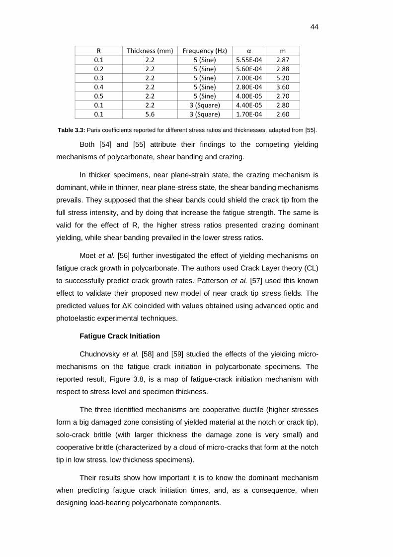
Chudnovsky et al. [58] and [59] studied the effects of the yielding micro-
mechanisms on the fatigue crack initiation in polycarbonate specimens. The
reported result, Figure 3.8, is a map of fatigue-crack initiation mechanism with
respect to stress level and specimen thickness.
The three identified mechanisms are cooperative ductile (higher stresses
form a big damaged zone consisting of yielded material at the notch or crack tip),
solo-crack brittle (with larger thickness the damage zone is very small) and
cooperative brittle (characterized by a cloud of micro-cracks that form at the notch
tip in low stress, low thickness specimens).
Their results show how important it is to know the dominant mechanism
when predicting fatigue crack initiation times, and, as a consequence, when
designing load-bearing polycarbonate components.
DBD
PUC-Rio - Certificação Digital Nº 1412756/CA
45
Figure 3.8: Map of crack initiation mechanism, adapted from [58].
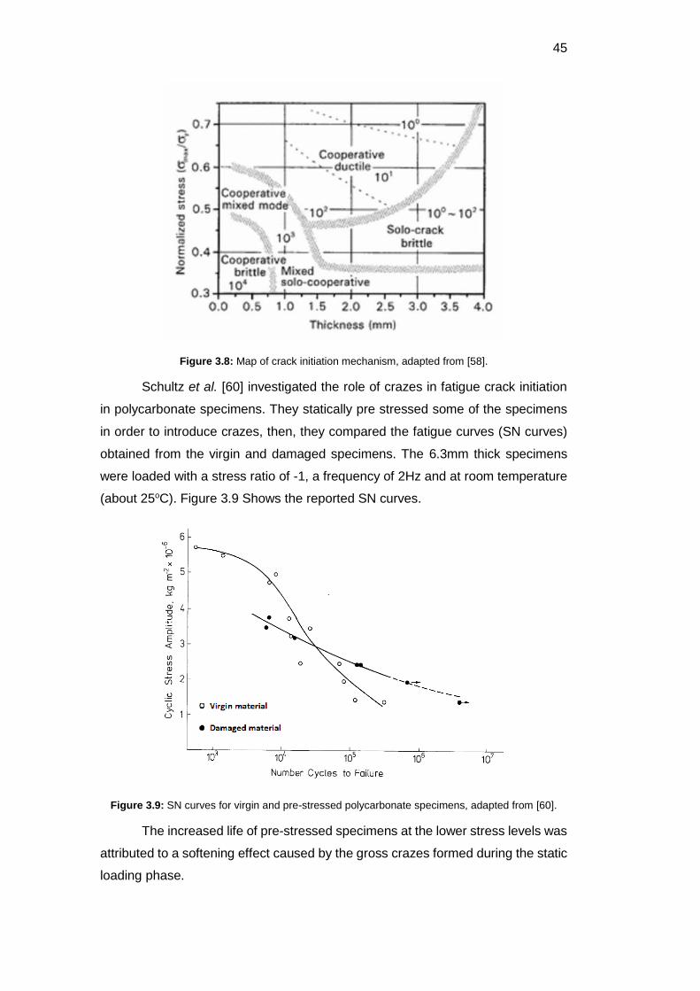
Schultz et al. [60] investigated the role of crazes in fatigue crack initiation
in polycarbonate specimens. They statically pre stressed some of the specimens
in order to introduce crazes, then, they compared the fatigue curves (SN curves)
obtained from the virgin and damaged specimens. The 6.3mm thick specimens
were loaded with a stress ratio of -1, a frequency of 2Hz and at room temperature
(about 25oC). Figure 3.9 Shows the reported SN curves.
Figure 3.9: SN curves for virgin and pre-stressed polycarbonate specimens, adapted from [60].
The increased life of pre-stressed specimens at the lower stress levels was
attributed to a softening effect caused by the gross crazes formed during the static
loading phase.
DBD
PUC-Rio - Certificação Digital Nº 1412756/CA

46
Chen et al. [61] also studied fatigue crack initiation in polycarbonate. They
used a damage model based on the fracture strain (εf) to predict the residual life of
6.3mm thick fatigue damaged specimens. The tests had a stress ratio of 0.1, at a
constant crosshead speed of 12.7mm/min and at room temperature. Figure 3.10(a)
shows their reported SN curve and Figure 3.10(b) shows the predicted damage
curve.
Figure 3.10: a) SN curve for polycarbonate specimens; b) Damage Curve, adapted from [61].
Meijer et al. [62] studied the differences between thermal and mechanical
failure of polycarbonate subjected to fatigue. In order to do that, they tested two
sets of specimens. The first set had isothermal conditions maintained through
water cooling, while the second set did not. Figure 3.11(a) shows the reported
results for isothermal fatigue and Figure 3.11(b) shows the results for non-
isothermal fatigue.
Figure 3.11: a) isothermal; b) non-isothermal fatigue curves for polycarbonate, adapted from [62].
DBD
PUC-Rio - Certificação Digital Nº 1412756/CA
47
At higher stress levels the temperature rises too much, and ductile failure
is caused by dissipative heat, at lower stress levels heat does not factor in the
failure process.
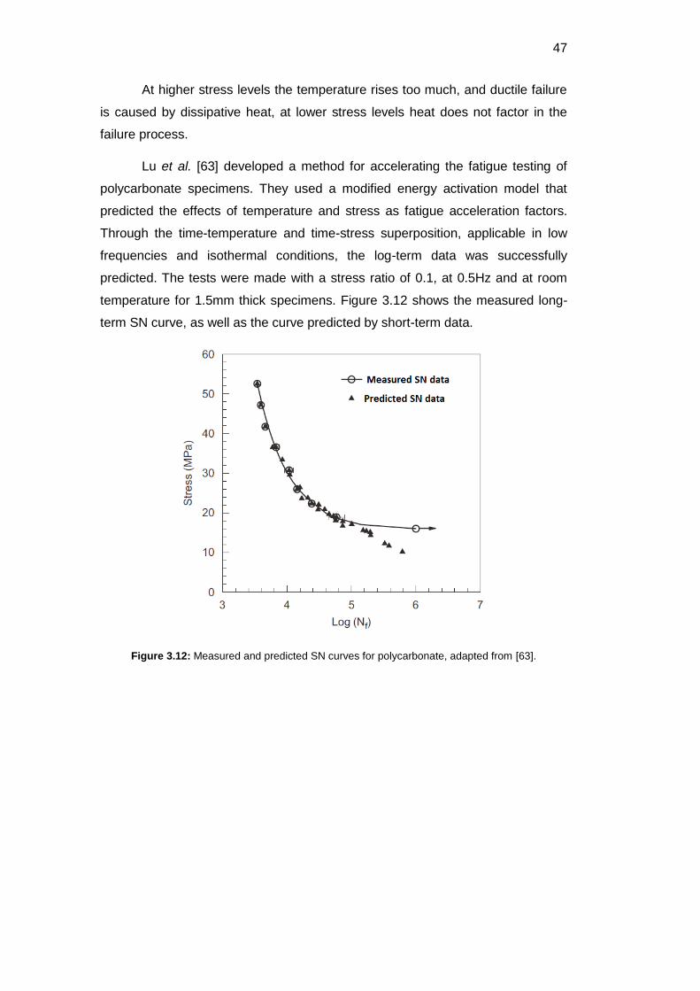
Lu et al. [63] developed a method for accelerating the fatigue testing of
polycarbonate specimens. They used a modified energy activation model that
predicted the effects of temperature and stress as fatigue acceleration factors.
Through the time-temperature and time-stress superposition, applicable in low
frequencies and isothermal conditions, the log-term data was successfully
predicted. The tests were made with a stress ratio of 0.1, at 0.5Hz and at room
temperature for 1.5mm thick specimens. Figure 3.12 shows the measured long-
term SN curve, as well as the curve predicted by short-term data.
Figure 3.12: Measured and predicted SN curves for polycarbonate, adapted from [63].
DBD
PUC-Rio - Certificação Digital Nº 1412756/CA

48
4
Pre-Experimental Work
4.1
Introduction
In this chapter, all the pre-experimental details are discussed. Such as,
specimen types, dimensions and preparation, loading machine and general
experimental procedures and cautions. Specific procedures are presented in
subsequent chapters, when needed.
4.2
The Specimens
Two types of specimens were used in the experiments described from here
on. The choice of the specimen types was made based on characteristics that
made possible the study of many fields at once.
The first type of specimen is the classic constant radius (CR tensile
specimen) (adapted from ASTM E466 - Standard Practice for Conducting Force
Controlled Constant Amplitude Axial Fatigue Tests of Metallic Materials). It consist
of a tensile specimen in which the gauge section is machined with a constant
radius, so that the middle cross-section is the critical one and a symmetry plane as
well. Figure 4.1 shows the dimensions of the specimens, machined from a 3.9mm
thick plate.
Figure 4.1: Dimensions of the constant radius specimens.
The second type of specimen is the keyhole, developed by SAE in the late
70’s. This specimen has a well documented stress concentration factor, similar to
typical components, it has a minimum of critical machining dimensions, and
permits studies of both crack initiation and propagation [64]. Figure 4.2 shows the
dimensions of the specimens, machined from a 3.9mm thick plate.
The stress concentration factor of the keyhole notch was firstly estimated
by that of a circular hole in an infinite plate Kt=3, since it was designed to simulate
this geometry. The Kt for the dimensions described in Figure 4.2 is calculated via
finite elements method and experimental techniques, as shown later.
DBD
PUC-Rio - Certificação Digital Nº 1412756/CA

49
Figure 4.2: Dimensions of the Keyhole specimens.
4.2.1
Loading Cautions
For the constant radius specimens, because of the holes made to fix the
specimen to the cyclic loading machine, the middle cross section no longer was
the critical section and fatigue cracks were initiating at the loading hole. To
remediate this problem, a custom grip was designed, which was able to transmit
the load to the specimen by friction, and consequently avoid the stress
concentration. Figure 4.3 shows a photo of a specimen mounted with the grips.
Figure 4.3: Constant radius specimen mounted with custom grips.
The loading of the keyhole specimens presented no problem, since the
stress concentration guaranteed that fatigue cracks initiated at the notch.
4.2.2
Specimen Preparation
As stated in chapter 2, polycarbonate is a very good choice for
thermography applications, since its infrared emissivity is naturally high. Because
of that, painting the specimens black was unnecessary and not much preparation
should be necessary.
The polycarbonate plate, from where all specimens were machined, was
bought from PALRAM Inc., it is called PALSUNTM and is designed to be used as
DBD
PUC-Rio - Certificação Digital Nº 1412756/CA

50
transparent roofs. They are extruded and rolled, having UV protection applied to
one side of the plate. The main material properties can be found on Appendix 3.
The UV protection, as expect, does not interfere with the infrared
measurements. This was tested by simply inverting the specimens, pointing the
camera to both sides and comparing the readings.
Thus, the only unknown property of the plate was the residual stresses
present due to the production process. The easiest way to circumvent this problem
was to submit the specimens to an annealing heat treatment, eliminating not only
the unknown pre-existing residual stresses, but the ones added in the machining
process as well. Figure 4.4 shows the isochromatic fringe patterns of an unloaded
specimen, (a) before annealing and (b) after annealing, in a photoelastic
transmission polariscope.
Figure 4.4: a)Specimen before annealing. b)After annealing.
The adapted annealing process consisted of a simplified version of what is
described in [65]. Basically, heating the specimen above its glass transition, at a
constant rate, keeping it at a constant temperature for a extended period of time,
and then cooling it slowly at a constant rate2. Table 4.1 show the temperatures and
times of the annealing heat treatment.
Process Temperatures (oC) Time (Hours)
Constant rate heating 25-160 4
Constant temperature 160 6
Constant rate cooling 160-25 4
Table 4.1: Temperatures and times of the adapted annealing heat treatment.
2 The annealing heat treatment was made in an electric circulation oven from Photolastic inc. coupled with a cam control unit from Partlow corp. (40-230ºC), which followed the temperatures described above, and a mercury-in-glass thermometer that was used to calibrate the temperature of the oven.
DBD
PUC-Rio - Certificação Digital Nº 1412756/CA

51
The specimens were covered in talcum powder, acting as a lubricant and
permitting free two-dimensional movement of the specimen between two glass
plates, which prevented non-uniform deformation. After annealing, the dimensions
of the specimens changed (about 1.7-2.0% in the preferential direction of the plate,
along the length of the CR specimen), because of the stress relief. The dimensions
reported before, in Figure 4.1 and Figure 4.2, were measured after annealing.
4.3
Cyclic Loading Machine
In order to study fatigue behavior, cyclic loading must be used. In the
present work, a pneumatic loading machine developed by [66] was used.
The machine, equipped with a servo valve3 controlled via a simple
computer program, applied a cyclic load with fixed frequency of 5Hz. The
magnitude of the load was controlled through three valves that regulated the
pressure of air entering the pneumatic muscle and how easily the air was expelled
after each cycle. A load cell4, connected in series with the specimen, was
responsible for feeding the load response to the program. Figure 4.5 shows a photo
of the setup with a CR tensile specimen mounted on the grips, while Figure 4.6
shows a screenshot of the controlling program.
Figure 4.5: Photo of the pneumatic loading machine setup.
3 Servo-valve – FESTO MHE4-MS1H-3/2G-1/4 (-0.9 – 8bar) 4 Load cell – MK Controle e Instrumentação Ltda. CSR-500 (5kN)
DBD
PUC-Rio - Certificação Digital Nº 1412756/CA
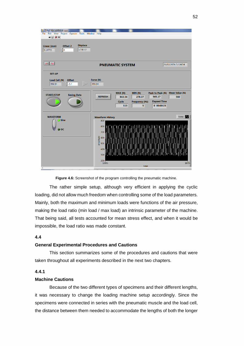
52
Figure 4.6: Screenshot of the program controlling the pneumatic machine.
The rather simple setup, although very efficient in applying the cyclic
loading, did not allow much freedom when controlling some of the load parameters.
Mainly, both the maximum and minimum loads were functions of the air pressure,
making the load ratio (min load / max load) an intrinsic parameter of the machine.
That being said, all tests accounted for mean stress effect, and when it would be
impossible, the load ratio was made constant.
4.4
General Experimental Procedures and Cautions
This section summarizes some of the procedures and cautions that were
taken throughout all experiments described in the next two chapters.
4.4.1
Machine Cautions
Because of the two different types of specimens and their different lengths,
it was necessary to change the loading machine setup accordingly. Since the
specimens were connected in series with the pneumatic muscle and the load cell,
the distance between them needed to accommodate the lengths of both the longer
DBD
PUC-Rio - Certificação Digital Nº 1412756/CA

53
CR tensile specimen and the shorter keyhole specimens. In order to do that, two
different length screws were used to connect the lower grip to the loading cell (as
can be seen in Figure 4.5).
Because of the differing lengths of these screws, their weights were
obviously different, and since the loading cell is connected at the bottom of the
setup, the load offset had to be set for each specimen. The load measurements
discounted the weight of the setup.
Another caution concerned the machine’s grips that had a fixed spacing,
which was different from the thickness of the polycarbonate specimens. That
generated a problem of misalignment of the specimens, resulting in bending
stresses. In the case of the CR tensile specimen this problem was circumvented
by the use of the custom grips (as discussed before). For the keyhole specimens,
spacers were added between the machine’s grips and the specimens, in order to
properly align them.
Lastly, because of the in-series setup of the machine, and the nature of the
pneumatic muscle, the load applied to the specimen was a function of the
specimen’s stiffness. The problem is that a direct correlation between air pressure
and load was not possible for all the experiments as a whole, but only for each
specific situation separately. For the CR tensile specimens where cracks were not
an issue and the stiffness was constant throughout the test, that was not much of
a problem. On the other hand, for the crack propagation tests using the keyhole
specimens, the air pressure needed to be constantly monitored and adjusted by
hand, in order to keep the desired load levels.
4.4.2
Infrared Camera Cautions
While using the infrared camera for either active or passive thermography
applications, there are some cautions to be taken. The cautions described here
are specific for the non-cooled, micro bolometer camera FLIR A655sc.
Firstly, when turning on the camera before each test, it is recommended to
wait some time until the camera itself reaches an equilibrium temperature. Around
10 to 15 minutes should be enough, and after that period of time the measurements
can be made for very long time. The camera has been used for over 8 hours
straight and measurements remained constant.
DBD
PUC-Rio - Certificação Digital Nº 1412756/CA

54
Another important aspect of the camera, specifically because of the
workings of the focal plane array, it has a high non-uniform response to radiation,
that means, each pixel is responding differently to the same level of infrared
radiation. The A655sc has an automatic non-uniformity correction (NUC)
procedure, which lowers a plate with very high emissivity in front of the detectors
and uses the data collected from it, at two different temperatures, to assign a gain
and an offset value to each pixel.
The manufacturer of the camera (FLIR Inc.) advises the use of this NUC
procedure every 15 to 30 minutes to guarantee the precision of the measurements.
The problem is that doing it in the middle of a test can throw off one’s results,
because the gain will change and early results will not be comparable to later ones,
since the value of these gains cannot be easily obtained. The advice from the TSA
software (Stress Photonics Inc.), which was followed and approved by this work,
is to turn off the automatic NUC procedure and run it manually before each test.
Additionally, although no effort to explain why it happens is made here, the author
of this work found out that after using the camera for more than 30 minutes or so
the NUC procedure barely changed the gains and offsets.
Lastly, a comment about the very high sensitivity of the camera and some
effects that arise from it that may not be obvious. Anything with temperature above
0K emits infrared radiation. Because of that, almost everything around a lab
environment can interfere in one’s results. Things like laptops, power supplies,
people walking around the lab and even the camera itself can emit considerable
amounts of radiation that may be reflected by the target and back to the detector.
This should not be a problem when making TSA measurements, because it uses
only temperature variations, but it certainly can be a huge problem when measuring
actual temperature values in active thermography, for example.
In order to minimize this problem, two cautions are advised. Placing the
camera right in front of a wall so that nothing is actually happening behind it, while
protecting the target and the surrounding area that is in front of the camera with
some kind of infrared opaque material, wood, cloth and styrofoam have been
successfully used for this purpose. Avoiding the camera’s own reflection can be
tricky, but can usually be accomplished by pointing the camera at the target at an
angle.
DBD
PUC-Rio - Certificação Digital Nº 1412756/CA

55
5
Thermography Applied to Fatigue Crack Initiation
This chapter is divided in four main parts concerning fatigue crack initiation
studies. Firstly, it discusses how to use thermography to locate critical points in a
component, then, an in-depth discussion on how to measure stress concentration
factors using TSA is made. Determination of fatigue limit is discussed next, laying
the theoretical ground for complete SN curve measurements through pure
thermography.
5.1
Locating Critical Points
In order to locate critical points, where fatigue is most likely to happen, there
are two possible approaches. The active thermography approach (exemplified in
Appendix 1) and the passive thermography approach, through TSA.
Considering that in most applications the critical point is located at a free
surface of the component, one of the principal stress components is equal to 0
(e.g. σ2=0) and the TSA data can be easily converted in the actual stress acting at
each point of the free surface. Then, the highest stress point, also the one with
highest TSA magnitude, is obviously the critical one. Difficulties may arise when a
more complicated stress field is present and the critical point might not be on a free
surface. In that case, some stress separation technique must be used, be it
numerical or experimental, in order to obtain the actual values of σ1 and σ2. Then,
a criterion such as Tresca’s or Mises’ should be used to combine these
components and determine which point is the critical one. Some of these
techniques are discussed in the next section. Figure 5.1 shows how easily the
critical points can be located in a cracked T-shaped specimen under cyclic loading
using TSA [17].
Figure 5.1: Cracked T-shaped specimen and critical points, adapted from [17].
DBD
PUC-Rio - Certificação Digital Nº 1412756/CA
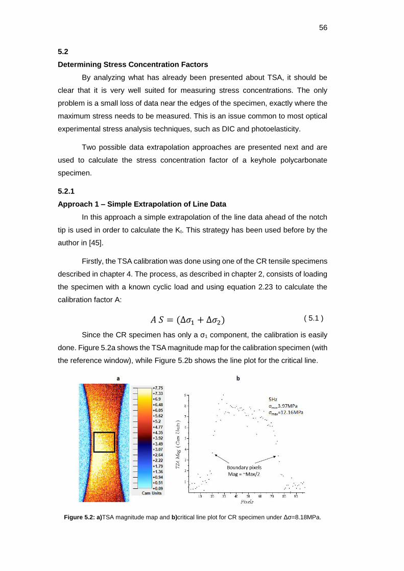
56
5.2
Determining Stress Concentration Factors
By analyzing what has already been presented about TSA, it should be
clear that it is very well suited for measuring stress concentrations. The only
problem is a small loss of data near the edges of the specimen, exactly where the
maximum stress needs to be measured. This is an issue common to most optical
experimental stress analysis techniques, such as DIC and photoelasticity.
Two possible data extrapolation approaches are presented next and are
used to calculate the stress concentration factor of a keyhole polycarbonate
specimen.
5.2.1
Approach 1 – Simple Extrapolation of Line Data
In this approach a simple extrapolation of the line data ahead of the notch
tip is used in order to calculate the Kt. This strategy has been used before by the
author in [45].
Firstly, the TSA calibration was done using one of the CR tensile specimens
described in chapter 4. The process, as described in chapter 2, consists of loading
the specimen with a known cyclic load and using equation 2.23 to calculate the
calibration factor A:
𝐴𝑆 = (∆𝜎1 + ∆𝜎2) ( 5.1 )
Since the CR specimen has only a σ1 component, the calibration is easily
done. Figure 5.2a shows the TSA magnitude map for the calibration specimen (with
the reference window), while Figure 5.2b shows the line plot for the critical line.
Figure 5.2: a)TSA magnitude map and b)critical line plot for CR specimen under Δσ=8.18MPa.
DBD
PUC-Rio - Certificação Digital Nº 1412756/CA
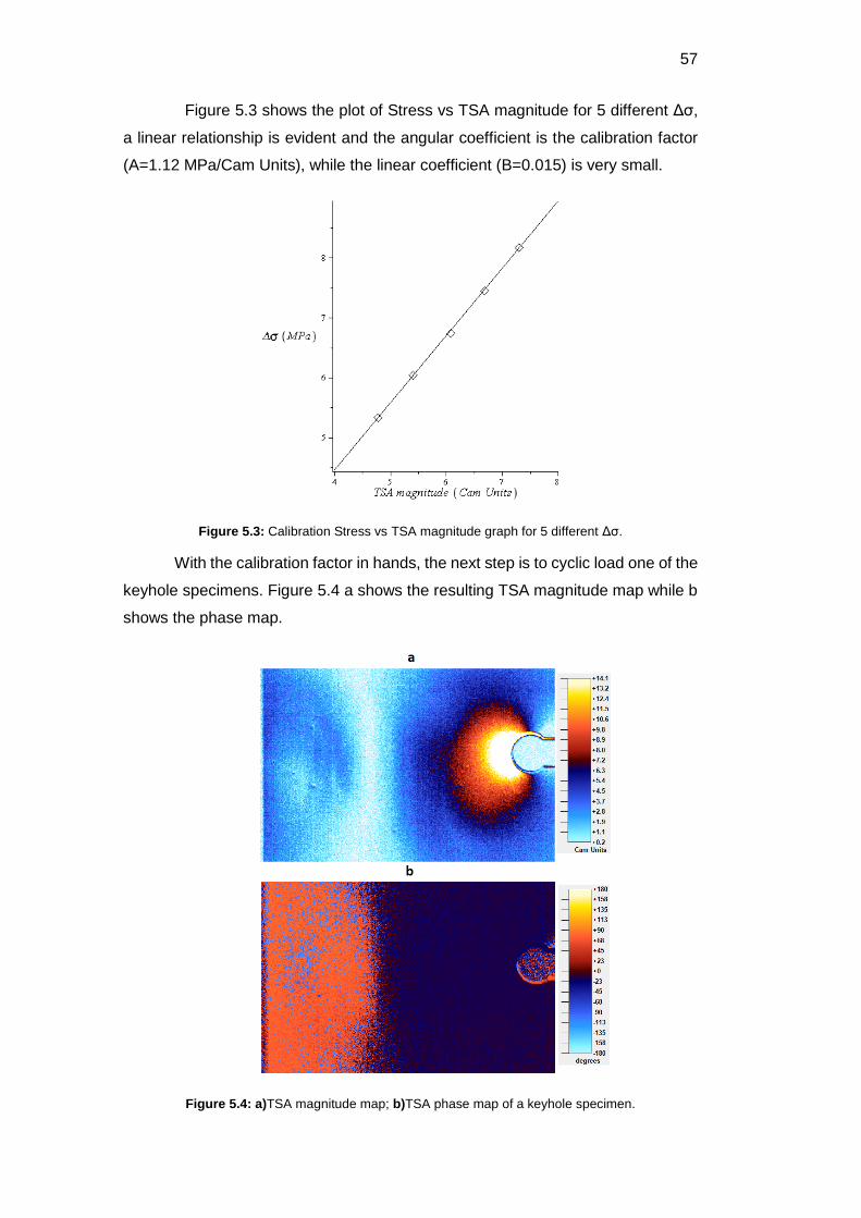
57
Figure 5.3 shows the plot of Stress vs TSA magnitude for 5 different Δσ,
a linear relationship is evident and the angular coefficient is the calibration factor
(A=1.12 MPa/Cam Units), while the linear coefficient (B=0.015) is very small.
Figure 5.3: Calibration Stress vs TSA magnitude graph for 5 different Δσ.
With the calibration factor in hands, the next step is to cyclic load one of the
keyhole specimens. Figure 5.4 a shows the resulting TSA magnitude map while b
shows the phase map.
Figure 5.4: a)TSA magnitude map; b)TSA phase map of a keyhole specimen.
DBD
PUC-Rio - Certificação Digital Nº 1412756/CA
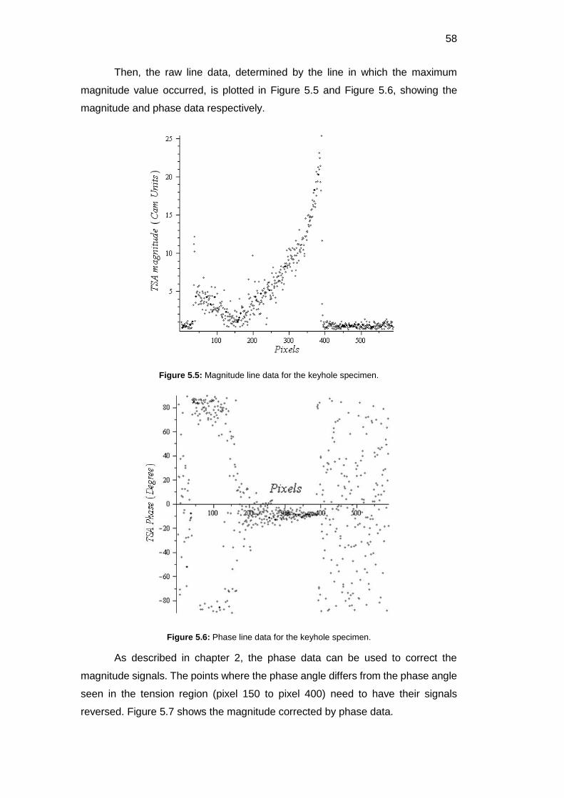
58
Then, the raw line data, determined by the line in which the maximum
magnitude value occurred, is plotted in Figure 5.5 and Figure 5.6, showing the
magnitude and phase data respectively.
Figure 5.5: Magnitude line data for the keyhole specimen.
Figure 5.6: Phase line data for the keyhole specimen.
As described in chapter 2, the phase data can be used to correct the
magnitude signals. The points where the phase angle differs from the phase angle
seen in the tension region (pixel 150 to pixel 400) need to have their signals
reversed. Figure 5.7 shows the magnitude corrected by phase data.
DBD
PUC-Rio - Certificação Digital Nº 1412756/CA

59
Figure 5.7: Magnitude data corrected by phase angle.
By excluding the points that are not part of the specimen’s surface, and
inverting the pixel numbers so that the pixel 0 is the one at the notch tip, the graph
in Figure 5.8 is the result.
Figure 5.8: Treated TSA data points for keyhole specimen.
The next step is to apply both the stress calibration of TSA and the length
scale. The length scale is simply determined by measuring the length of the section
ahead of the notch (60.5mm) and dividing it by the number of pixels in Figure 5.8
(353 pixels), giving a length scale of 0.1714 mm/pixel. Figure 5.9 shows the
normalized stress vs distance from notch plot, with ΔP=420N (the cyclic load) and
R=4.3mm (the radius of the notch).
DBD
PUC-Rio - Certificação Digital Nº 1412756/CA

60
Figure 5.9: Normalized stress vs distance from notch plot for keyhole.
Figure 5.10 shows the resulting extrapolation using the data points from
pixel 1 to pixel 100 to fit a curve following equation 5.2 5
𝛥𝜎
𝛥𝑃=
𝐶0
(1 + 𝑥/𝑅)ℎ+ 𝐶1 + 𝐶2(1 + 𝑥/𝑅)
( 5.2 )
where the coefficients C0, C1 and C2, as well as the exponent h are fitting
parameters to be determined via the minimum squared error method.
Figure 5.10: Curve-fitted TSA data for keyhole specimen.
5 This equation was chosen because of the expected 1/xh dependency of the stresses. The other terms were added in order to fit the data farther from the notch tip.
DBD
PUC-Rio - Certificação Digital Nº 1412756/CA

61
From the fitted curve, the maximum stress at the notch tip can be
determined and used to calculate the stress concentration factor. The maximum
stress was (Δσ/ΔP)max= 0.0864, and the nominal stress was calculated as the sum
of the tensile and bending stresses via equation 5.3
(𝛥𝜎
𝛥𝑃)𝑛𝑜𝑚
=1
𝑡𝑏+1(𝐵 − 𝐻𝑏 −
𝑏2) (
𝑏2)
𝑡𝑏3
12
= 0.0292
( 5.3 )
where t is the specimen thickness (3.9mm), b is the length of the section ahead of
the notch (60.5mm), B is the total width (116mm) and Hb is the horizontal distance
of the loading pin to the border (26.25mm). Then, (with a fitting exponent h of
~0.65) the resulting Kt is:
𝐾𝑡 = (𝛥𝜎
𝛥𝑃)𝑚𝑎𝑥
(𝛥𝜎
𝛥𝑃)𝑛𝑜𝑚
⁄ = 2.95 ( 5.4 )
5.2.2
Approach 2 – Stress Function and Principal Stresses Separation
In order to obtain better results and showcase the power of hybrid TSA, this
approach uses an Airy’s stress function to fit the TSA data in an area around the
notch. By doing this, the stress components are determined and the Kt calculated.
Instead of collecting the data only from the line ahead of the notch tip, the
procedure now collects data from the whole area show in Figure 5.11, measuring
315 pixels long and 127 pixels wide, leaving a minimum of 6 pixels between
collected data and the borders of the specimen6.
Figure 5.11: Area, in gray, for stress function fitting.
The stress function used to fit the data was adapted from [19] and is
reproduced in equation 5.5 below:
6 The dimensions are given in pixels because in each experiment the distance from the camera to the specimen is different. The algorithms only translate the lengths to mm at the end of computations.
DBD
PUC-Rio - Certificação Digital Nº 1412756/CA

62
𝛷 = 𝑏0 ln(𝑟) + 𝑐0𝑟2 + (
𝑐′1𝑟+ 𝑑′1𝑟
3) cos(𝜃)
+∑[(𝑎′𝑛𝑟𝑛 + 𝑏′𝑛𝑟
𝑛+2 + 𝑐′𝑛𝑟−𝑛 + 𝑑′𝑛𝑟
2−𝑛)cos(𝑛𝜃)]
𝑁
𝑛=2
( 5.5 )
where b0, c0, c’1, d’1, a’n, b’n, c’n and d’n are the fitting coefficients that are later
determined via least mean squares method, r and θ are the polar coordinates of
each point with respect to the origin at the center of the notch. N is one fourth of
the number of terms minus 4 terms (b0, c0, c’1, d’1).
Then, using equation 3.10, repeated here as equation 5.6, the stress
components can be determined for all points of the specimen.
𝜎𝜃 =𝜕2𝛷
𝜕𝑟2
𝜎𝑟 =1
𝑟
𝜕𝛷
𝜕𝑟+
1
𝑟2𝜕2𝛷
𝜕𝜃2
𝜎𝑟𝜃 = −𝜕
𝜕𝑟(1
𝑟
𝜕𝛷
𝜕𝜃)
( 5.6 )
For the results shown, 84 terms (N=20) were used in the fitting of 31328
experimental data points and 30060 boundary condition points evenly distributed
as σr=σrθ=0 at the notch border, σx=σxy=0 at the back free surface and σy=σxy=0 at
both the slit’s free surfaces . Figure 5.12 shows the tangential stress (σθ)
distribution.
Figure 5.12: Fitted σθ field.
DBD
PUC-Rio - Certificação Digital Nº 1412756/CA
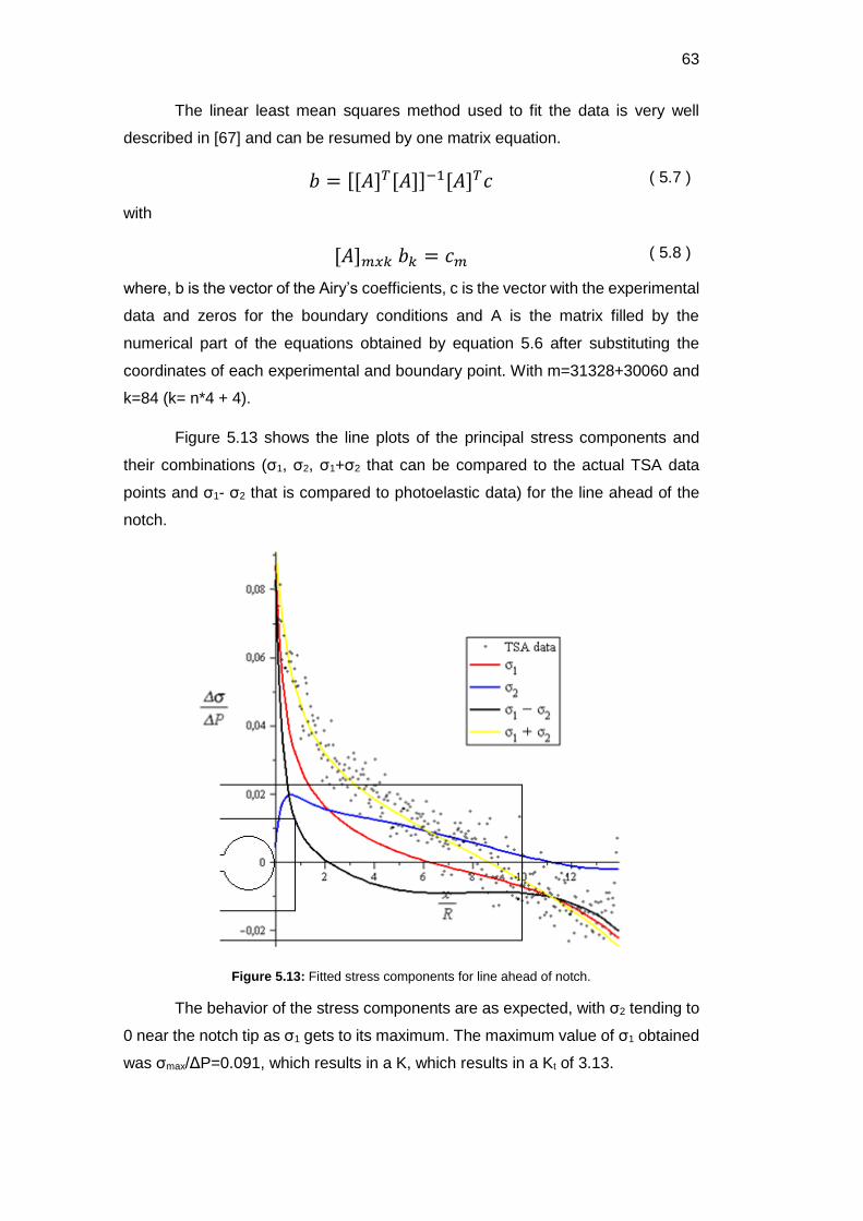
63
The linear least mean squares method used to fit the data is very well
described in [67] and can be resumed by one matrix equation.
𝑏 = [[𝐴]𝑇[𝐴]]−1[𝐴]𝑇𝑐 ( 5.7 )
with
[𝐴]𝑚𝑥𝑘 𝑏𝑘 = 𝑐𝑚 ( 5.8 )
where, b is the vector of the Airy’s coefficients, c is the vector with the experimental
data and zeros for the boundary conditions and A is the matrix filled by the
numerical part of the equations obtained by equation 5.6 after substituting the
coordinates of each experimental and boundary point. With m=31328+30060 and
k=84 (k= n*4 + 4).
Figure 5.13 shows the line plots of the principal stress components and
their combinations (σ1, σ2, σ1+σ2 that can be compared to the actual TSA data
points and σ1- σ2 that is compared to photoelastic data) for the line ahead of the
notch.
Figure 5.13: Fitted stress components for line ahead of notch.
The behavior of the stress components are as expected, with σ2 tending to
0 near the notch tip as σ1 gets to its maximum. The maximum value of σ1 obtained
was σmax/ΔP=0.091, which results in a K, which results in a Kt of 3.13.
DBD
PUC-Rio - Certificação Digital Nº 1412756/CA

64
For verification purposes, the stress concentration factor was measured via
DIC and Photoelasticity, as well as calculated through the finite elements method.
The procedures are described in Appendix 4 and Appendix 5. Table 5.1 shows the
results obtained.
TSA ap1 TSA ap2 DIC Photoelasticity FEM Literature [64]
Kt 2.95 3.13 3.27 3.25 3.02 3 - 3.25
Table 5.1: Results for the Kt of the keyhole specimen.
Finally, Figure 5.14 shows the line plots ahead of the notch, obtained by
the TSA approach 2, DIC and Photoelasticity measurements.
Figure 5.14: TSA, DIC and Photoelasticity results for the line ahead of notch.
5.3
Measuring Fatigue Limit Using Thermography
As pointed before, measuring the fatigue limit of a material in the traditional
way takes a very long time. Risitano et al. [68] proposed a methodology for the
rapid determination of this property using thermography.
The idea behind the method is based on the reported rise in temperature of
a specimen cyclic loaded above the fatigue limit. This temperature rise is usually
explained by a combination of the thermoelastic effect and internal damping within
the elastic field.
DBD
PUC-Rio - Certificação Digital Nº 1412756/CA

65
When a specimen is cyclic loaded, the temperature (T) vs number of cycles
(N) curve is similar to the one show in Figure 5.15 [69].
Figure 5.15: T vs N curve for cyclic load above the fatigue limit, adapted from [69].
The curve clearly shows three phases. Phase 1, where the temperature
rises, and in this region, the rate of heating is higher for higher stresses. Phase 2,
where the temperature stabilizes. The stabilization temperature is higher for higher
stresses. Finally, phase 3, where the temperature rapidly rises again, and final
failure is imminent.
The idea is to measure the stabilization temperature of several different
stress levels, from lower to higher, in a single specimen. Then, subtract the initial
temperature of the specimen and use an unloaded specimen placed by its side as
the ambient temperature reference and use equation 5.9 to calculate the data
points for each stress level.
𝑇(𝑛) = (𝑇𝑚𝑎𝑥(𝑛) − 𝑇𝑎𝑚𝑏(𝑛)) − ((𝑇𝑚𝑎𝑥(1) − 𝑇𝑎𝑚𝑏(1))) ( 5.9 )
where T(n) is the temperature elevation at the cycle n, Tmax(n) is the maximum
temperature of the observed area on the surface of the loaded specimen at cycle
n, Tamb(n) is the temperature of the surface of the reference specimen at cycle n,
Tmax(1) and Tamb(1) are the maximum and reference temperatures at the first cycle.
The CR tensile specimen is cyclic loaded in a stair case pattern, as shown
in Figure 5.16. Because of the loading machine limitations, described in chapter 4,
the mean load was not constant, and the Goodman’s relationship was used to
account for that. Figure 5.17 shows the T(n) vs n curve for the first, fifth, seventh
and ninth stress levels, while Figure 5.18 shows two thermographic images
obtained before loading and during the 7th load level.
DBD
PUC-Rio - Certificação Digital Nº 1412756/CA

66
Figure 5.16: Loading steps for fatigue limit evaluation.
Figure 5.17: T(n) vs cycles points for 4 different load levels.
DBD
PUC-Rio - Certificação Digital Nº 1412756/CA
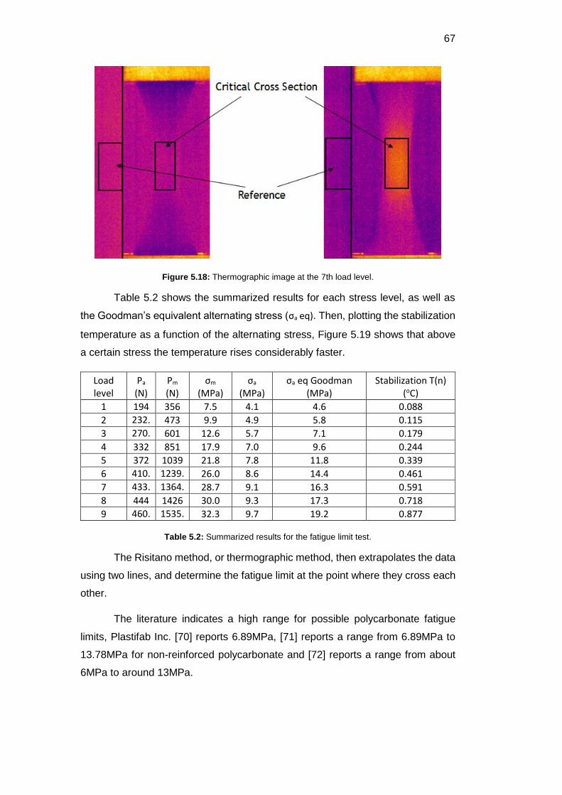
67
Figure 5.18: Thermographic image at the 7th load level.
Table 5.2 shows the summarized results for each stress level, as well as
the Goodman’s equivalent alternating stress (σa eq). Then, plotting the stabilization
temperature as a function of the alternating stress, Figure 5.19 shows that above
a certain stress the temperature rises considerably faster.
Load level
Pa (N)
Pm (N)
σm (MPa)
σa (MPa)
σa eq Goodman (MPa)
Stabilization T(n) (oC)
1 194 356 7.5 4.1 4.6 0.088
2 232.5
473 9.9 4.9 5.8 0.115
3 270.5
601 12.6 5.7 7.1 0.179
4 332 851 17.9 7.0 9.6 0.244
5 372 1039 21.8 7.8 11.8 0.339
6 410.5
1239.5
26.0 8.6 14.4 0.461
7 433.5
1364.5
28.7 9.1 16.3 0.591
8 444 1426 30.0 9.3 17.3 0.718
9 460.5
1535.5
32.3 9.7 19.2 0.877
Table 5.2: Summarized results for the fatigue limit test.
The Risitano method, or thermographic method, then extrapolates the data
using two lines, and determine the fatigue limit at the point where they cross each
other.
The literature indicates a high range for possible polycarbonate fatigue
limits, Plastifab Inc. [70] reports 6.89MPa, [71] reports a range from 6.89MPa to
13.78MPa for non-reinforced polycarbonate and [72] reports a range from about
6MPa to around 13MPa.
DBD
PUC-Rio - Certificação Digital Nº 1412756/CA

68
Figure 5.19: T(N) vs σa eq for polycarbonate.
The resulting fatigue limit is σ0= 13.8MPa. Although this result agrees with
what was found in the literature, it is in the high-end of the possible spectrum, and
the author believes that it should not be the case7. Errors of about ±15% have been
reported in the application of the thermographic method [68], which would give a
possible range of fatigue limit for polycarbonate from 11.7MPa to 15.9MPa :
𝜎0 = 13.8 ± 15% ( 5.10 )
5.4
Determination of the Fatigue Curve Using Thermography
Risitano et al. [69] proposed a method, based on the methodology to
measure the fatigue limit, to determine the whole fatigue curve of a material using
thermography. This method, once again, is much faster than the traditional method
to bring up this data, and needs theoretically only one specimen. In practice, three
specimens is the recommended minimum.
The main idea behind this method is an energy approach to damage
𝐸𝑐 = ∫ 𝐸𝑝
𝑁𝑓
0
𝑑𝑁
( 5.11 )
7 If instead of using Goodman’s model, the Gerber’s model for equivalent stress was used, the resulting fatigue limit would be 9.6MPa. Nonetheless, the Goodman’s equation is used throughout this work since it is more oftenly used in the polycarbonate literature.
DBD
PUC-Rio - Certificação Digital Nº 1412756/CA

69
where, Ec is the amount of micro-plastic deformation energy to failure per unit
volume, a material property, Nf is the number of cycles to failure and Ep is the
energy due to yielding per unit volume per cycle.
The argument of energy equilibrium is then used,
𝐸𝑤 = 𝐸𝑖 + 𝑄 ( 5.12 )
balancing the work done over the system by the loading (Ew), the stored internal
energy (Ei) and the energy converted into heat (Q). Assuming Ei to be small
compared to Q, and using Risitano’s results, which have shown Ew to be
proportional to Ep, the authors of [69] proposed
𝐸𝑐 = ∫ 𝑑𝑄
𝑇𝑓
0
( 5.13 )
For small temperature variations (under 100K, implies small loading
frequencies), the heat transferred from the specimen to the environment can be
considered proportional to the temperature difference T(n). Because of that, Q can
be evaluated through a parameter Φ, which is the integral of the T vs N curve of
Figure 5.15.
𝑄𝛼𝛷𝛼𝐸𝑐 ( 5.14 )
with
𝛷 = ∫ 𝑇(𝑛)𝑑𝑁
𝑁𝑓
0
( 5.15 )
or, approximately, the sum of the areas below the curve, neglecting phase 3, which
is normally very fast.
𝛷 =𝑇2𝑁𝑠
2+ 𝑇2(𝑁𝑓 −𝑁𝑠) = 𝑐𝑜𝑛𝑠𝑡𝑎𝑛𝑡
( 5.16 )
where T2 is the stabilization temperature, Ns is the number of cycles until the
temperature stabilizes and Nf is the number of cycles to failure.
In practice, Φ is used as a (material property) critical value that would take
a specimen to fatigue failure, and measurements of T2 and Ns at various stress
levels for a single specimen could yield the whole fatigue curve.
DBD
PUC-Rio - Certificação Digital Nº 1412756/CA

70
Figure 5.20 illustrates how the measurements process takes place, and
makes the method easy to grasp.
Figure 5.20: Illustration of the testing procedure for Risitano method, adapted from [69].
The specimen is loaded in a stair case mode, with various stress levels (σi),
for each one of those a Ns i is measured as indicated in Figure 5.20
𝑁𝑠𝑖 =𝛥𝑁𝑖 𝑇𝑖
𝑇𝑖 − 𝑇𝑖−1 ( 5.17 )
where ΔNi and Ti are the number of cycles from the start of a stress level until
stabilization and the stabilization temperature for each level, respectively.
For each σi, with the respective Ti and Ns i, assuming Φ has been previously
measured, equation 5.16 can be used to determine Nf I (doing T2=Ti and Ns=Ns i),
and each pair (Nf i , σi) is a point in the fatigue SN curve of the material.
Theoretically, Φ could be measured within the same specimen, if it was
taken to failure it would only require integrating the curve shown in Figure 5.20. In
this work, the value of Φ was measured with a CR tensile specimen loaded with a
constant cyclic stress level until failure, and two subsequent specimens were used
to gather data points for the fatigue curve.
5.4.1
Φ Determination
In order to determine Φ, a fatigue test with constant loading range was
conducted. The thermographic image obtained in the test is similar to that of Figure
5.18. The procedure follows the one described for fatigue limit calculation, the only
difference being that the load was kept constant at Pm=1637N and Pa=477N, which
DBD
PUC-Rio - Certificação Digital Nº 1412756/CA

71
results in a Goodman equivalent stress of 21.25MPa, and a measured total life (Nf)
of 24250 cycles.
Figure 5.21 shows the T(n) vs cycles graph obtained from the test, and the
three phases described before are clearly seen.
Figure 5.21: T(n) vs cycles graph for Φ measurement (~25000cycles = approximately 1.5h test).
The stabilization time (Ns) was determined visually as 1500 cycles, the
stabilization temperature (T2) was taken as the mean value of T(n) after the first
1500 cycles which resulted in 1.23ºC. Then, using equation 5.16, the value of Φ is
28905 ºC cycles.
5.4.2
SN curve determination
Having determined the value of Φ, the determination of the SN curve
through equations 5.16 and 5.17 requires a specimen to be cyclic loaded in a
staircase mode.
Table 5.3 shows the loading conditions, the visually determined Ti’s and
ΔNi’s, as well as the resulting Goodman‘s equivalent stress, Ns i‘s and Nf i’s for the
first specimen, which was loaded until failure in one go.
Figure 5.22 shows the T(n) vs cycles graph, the horizontal lines define the
value of Ti for each stress level. The integration of all points gives a Φ value of
26560, close to the calculated before, demonstrating that the procedure could be
done with a single specimen.
DBD
PUC-Rio - Certificação Digital Nº 1412756/CA

72
Pa
(N) Pm (N)
σa
(MPa)
σm
(MPa)
σa eq Goodman
(MPa)
Ti (oC)
ΔNi (cycles)
Ns i (cycles)
Nf i (cycles)
405 1161 8.51 24.39 13.62 0.59 1125 1125 49637
430.5 1310.5 9.04 27.53 15.69 0.69 975 6550 45045
451.5 1447.5 9.49 30.41 17.83 0.99 1725 5799 32245
473.5 1591.5 9.95 33.44 20.49 1.02 1125 29538 42997
498 1758 10.46 36.93 24.23 1.34 1375 5873 24556
508 1832 10.67 38.49 26.17 1.39 950 25376 33498
512 1875 10.76 39.39 27.30 1.44 1000 27207 33649
532.5 2021.5 11.19 42.47 32.28 1.76 750 4205 18573
550 2174 11.56 45.67 38.87 2.18 575 2949 14734
560.5 2276.5 11.78 47.83 44.57 2.49 500 4004 13606
567.5 2367.5 11.92 49.74 50.79 2.90 250 1787 10875
Table 5.3: Results of first specimen for SN curve determination.
Figure 5.22: T(n) vs cycles graph of first specimen for SN curve determination.
With the second specimen a different approach was used. Instead of
loading the specimen until failure in one go, two loading procedures were used in
two different tests, in order to study the effect of pre-existing damage on the
specimen.
Table 5.4 and Figure 5.23 show the results for both tests.
The integration of all points results in a Φ value of 25430, again close to the
originally calculated.
DBD
PUC-Rio - Certificação Digital Nº 1412756/CA

73
Test 1
Pa
(N) Pm (N)
σa
(MPa)
σm
(MPa)
σa eq Goodman
(MPa)
Ti (oC)
ΔNi (cycles)
Ns i (cycles)
Nf i (cycles)
439.5 1364.5 9.23 28.67 16.52 0.71 1100 1100 42233
468 1547 9.83 32.50 19.67 0.95 750 2938 32512
496.5 1760.5 10.43 36.99 24.20 1.25 700 2936 25111
518.5 1922.5 10.89 40.39 28.77 1.60 750 3406 20139
534.5 2046.5 11.23 43.00 33.17 1.90 625 3965 17512
543.5 2138.5 11.42 44.93 36.98 2.08 300 3619 16052
556.5 2260.5 11.69 47.49 43.41 2.44 300 2024 13144
Test 2
Pa
(N) Pm (N)
σa
(MPa)
σm
(MPa)
σa eq Goodman
(MPa)
Ti (oC)
ΔNi (cycles)
Ns i (cycles)
Nf i (cycles)
428.5 1311.5 9.00 27.55 15.63 0.73 1375 1375 41282
472.5 1594.5 9.93 33.50 20.48 1.05 625 2029 29107
503.5 1803.5 10.58 37.89 25.36 1.41 575 2246 22023
527 1987 11.07 41.75 30.95 1.74 400 2124 18027
535 2064 11.24 43.36 33.77 1.97 225 1959 15996
550 2193 11.56 46.07 39.69 2.28 150 1099 13517
Table 5.4: Results of second specimen for SN curve determination.
Figure 5.23: T(n) vs cycles graphs of second specimen for SN curve determination.
By taking all the (Nf I, σa eq) pairs, the resulting SN graph is shown in Figure
5.24 below. The points are plotted in a log-log scale and are fitted by a parabolic
relationship like equation 3.1. The resulting equation is:
𝑁𝑆1.316 = 1.75 ∗ 106 ( 5.18 )
where N is the number of cycles and S is the Goodman equivalent stress.
DBD
PUC-Rio - Certificação Digital Nº 1412756/CA

74
Figure 5.24: SN curve measured via thermography.
5.4.3
SN curve verification
In order to verify the validity of the obtained SN curve, traditional method
points are added to the graph, as well as literature results described in Chapter 2.
Figure 5.25 shows the resulting plot with all the data.
Figure 5.25: SN curve with all data points.
DBD
PUC-Rio - Certificação Digital Nº 1412756/CA

75
The traditional method points consist of 3 CR tensile specimens
(21.25MPa, 10.54MPa and 9.21MPa) and 3 keyhole specimens (13.64MPa,
16.09MPa and 17.31MPa) that had cracks initiated with constant load parameters.
Using Goodman’s relationship to calculate the equivalent alternating stress and
counting the cycles to failure (for the CR tensile specimens) or until a visible crack
was detected (for the keyhole specimens), each specimen represents a single
point in the graph.
The points signaled as 1 and 2 call for special explanations. Point 1 was
loaded with an equivalent stress (10.54MPa) lower than what was measured as
the fatigue limit, but it still broke at about 55700 cycles. Point 2 was loaded with a
slightly lower equivalent stress (9.21MPa) and did not fail up to 680000 cycles. The
fact that the test frequency was kept at 5Hz made going any longer than this a
counter-productive choice.
The reference results, taken from literature, are shown as solid symbols on
the plot. The results show decent similarity. The differences can be explained by
test parameters such as load ratio, thickness, frequency and the material
properties. It is very hard to compare the results effectively, since yield strength
values were not reported, Chen did not report the loading frequency, Schultz had
varying frequencies and the thicknesses are not equal. Nonetheless, the
counterintuitive result reported by [54] and [55], about the stress ratio effect seems
to be in effect here as well (See page 39).
DBD
PUC-Rio - Certificação Digital Nº 1412756/CA

76
6
Thermography Applied to Fatigue Crack Growth
This chapter is divided into two main parts concerning fatigue crack growth.
The measurement of stress intensity factors (SIF’s) using TSA is addressed first.
Two similar algorithms, one with a linear and the other with a non-linear approach,
are presented as an automatic KI measuring technique. Then, using the non-linear
algorithm, the da/dN curve is single handedly determined through TSA.
Before measuring a crack’s SIF, it is necessary to find the crack and locate
its tip. Appendix 2 shows a brief experiment on that, and highlights how easy it is
to follow the propagating crack tip, by looking for the points with higher stresses.
6.1
Measuring Stress Intensity Factors Using TSA
Many authors have used TSA to measure SIF’s, and used varied numerical
and experimental approaches. Stanley and Chan [73] used the first two terms of
the Westergaard’s stress function to fit the thermoelastic data around cracks in
mode I and II. Stanley and Dulieu-Smith [74] based their approach on the cardioid
format of the isopachic fringes around a crack tip. Lesniak et al. [75] used Williams’
stress field equations to fit the data using the least squares method (LSM). Lin et
al. [37] approached the problem using the J-integral formulation in the data fitting
process. Tomlinson et al. [35] developed a technique based on Muskhelishvili’s
stress field equations and a multipoint-over-deterministic method (MPODM). Díaz
et al. [76] and [77] proposed a methodology for finding the crack tip position by
looking at thermoelastic data, and then fitting the data using a non-linear approach
in order to measure SIF’s of propagating cracks. Marsavina et al. [40] used TSA to
investigate crack closure during fatigue. Tomlinson and Olden [34] presented a
broad review on the use of TSA in fracture mechanics and fatigue cracks.
The present work falls in line with these previous authors and attempts to
develop an automated technique that can be used with a non-expensive infrared
camera in combination with DeltaTherm2 software, as described in chapter 2.
6.1.1
The SIF Calculation Algorithm
Figure 6.1 shows a flowchart of the SIF calculation algorithm. The following
sections describe each step.
DBD
PUC-Rio - Certificação Digital Nº 1412756/CA
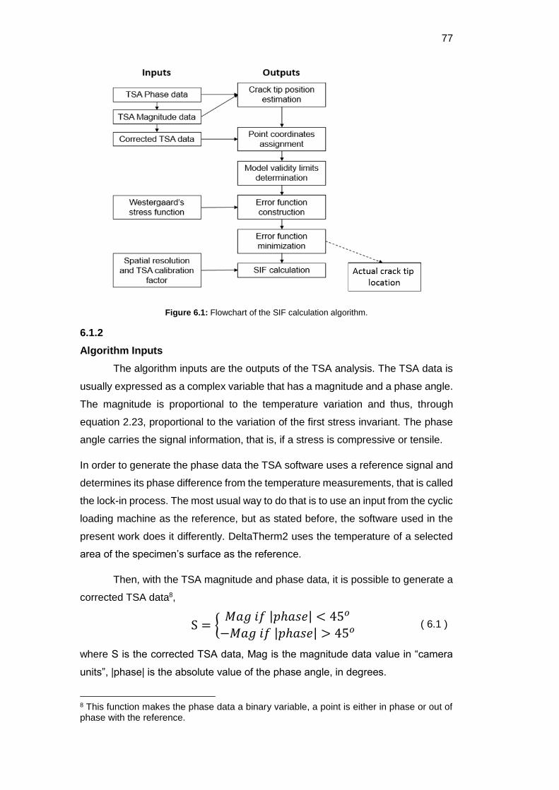
77
Figure 6.1: Flowchart of the SIF calculation algorithm.
6.1.2
Algorithm Inputs
The algorithm inputs are the outputs of the TSA analysis. The TSA data is
usually expressed as a complex variable that has a magnitude and a phase angle.
The magnitude is proportional to the temperature variation and thus, through
equation 2.23, proportional to the variation of the first stress invariant. The phase
angle carries the signal information, that is, if a stress is compressive or tensile.
In order to generate the phase data the TSA software uses a reference signal and
determines its phase difference from the temperature measurements, that is called
the lock-in process. The most usual way to do that is to use an input from the cyclic
loading machine as the reference, but as stated before, the software used in the
present work does it differently. DeltaTherm2 uses the temperature of a selected
area of the specimen’s surface as the reference.
Then, with the TSA magnitude and phase data, it is possible to generate a
corrected TSA data8,
S = {𝑀𝑎𝑔𝑖𝑓|𝑝ℎ𝑎𝑠𝑒| < 45𝑜
−𝑀𝑎𝑔𝑖𝑓|𝑝ℎ𝑎𝑠𝑒| > 45𝑜 ( 6.1 )
where S is the corrected TSA data, Mag is the magnitude data value in “camera
units”, |phase| is the absolute value of the phase angle, in degrees.
8 This function makes the phase data a binary variable, a point is either in phase or out of phase with the reference.
DBD
PUC-Rio - Certificação Digital Nº 1412756/CA
78
Other input needed is the mathematical model used. In this case, a
Westergaard’s stress function (We) was used to describe the stress field around
the crack tip [67],
𝑊𝑒(𝑥, 𝑦) = 𝜎1 + 𝜎2 = 2[𝑅𝑒(𝑍) + 𝑅𝑒(𝑌)] ( 6.2 )
with,
Z = ∑[𝐴𝑛𝑧𝑛−0.5]
𝑁
𝑛=0
𝑌 = ∑[𝐵𝑚𝑧𝑚]
𝑀
𝑚=0
( 6.3 )
where N and M determine the number of coefficients to be used, An and Bm are the
data fitting coefficients and z is the complex variable of the point coordinates
𝑧 = (𝑥 − 𝑥𝑜) + 𝑖(𝑦 − 𝑦𝑜) ( 6.4 )
being x and y the horizontal and vertical coordinates of a point (placing the origin
at the estimated crack tip location and the x axis along the crack propagation
direction). i= √-1, and xo and yo the horizontal and vertical errors of the estimated
crack tip location, which are solved for only when applying the non-linear method;
for the linear method they are set to 0.
The last inputs needed are the spatial resolution (SR) and the TSA
calibration factor (A). The spatial resolution is simply determined via a known
dimension in the specimen,
𝑆𝑅 = 𝑊
𝑝⁄ ( 6.5 )
where SR is the spatial resolution in mm/pixel, W is a known dimension of the
specimen in mm (e.g. width) and p is the number of pixels the dimension measures
on the thermographic image. The TSA calibration process is discussed in chapter
2 and the experiment presented in chapter 5.
6.1.3
Crack Tip Position Estimation and Point Coordinates Assignment
This work uses an specially improved and automated version of the
methodology proposed in [76] to estimate the position of the crack tip.
Firstly, the image needs to be positioned so that the crack is horizontal.
Then, using the TSA magnitude map, the vertical position of the crack tip (Yo’) is
DBD
PUC-Rio - Certificação Digital Nº 1412756/CA

79
estimated by plotting y vs 1/S2 curves for each vertical line in the image
(perpendicular to the crack). The resulting graphs, for the lines ahead of the crack
tip, have a clear minimum value. The mean value of y where this minimum value
occurs for all the vertical lines is equal to Yo’. Figure 6.2a shows the magnitude
map around a crack, while Figure 6.2b shows a typical y vs 1/S2 plot.
Figure 6.2: a)The magnitude map around a crack and b)Typical y vs 1/S2 plot.
The horizontal position of the crack tip (Xo’) is estimated through what is
called the phase shift. Due to the plasticity near the crack tip, the adiabatic
conditions required by TSA are lost. This can be seen as an abrupt change in
phase angle right in front of the crack tip. In the horizontal phase vs x curve at Yo’,
the position where this abrupt change occurs is equal to Xo’. Figure 6.3a shows the
phase map around a crack and Figure 6.3b shows a typical phase vs x plot.
Figure 6.3: a)The phase map around a crack and b)Typical phase vs x plot.
DBD
PUC-Rio - Certificação Digital Nº 1412756/CA

80
Having the values of Xo’ and Yo’, the coordinates assignment step is simple,
each point of the image gets assigned to an x and a y value, which are the
horizontal and vertical distances from the estimated crack tip, respectively.
6.1.4
Model Validity Limits Verification
The points used for the data fitting process must be in accordance with the
mathematical model. In [77], the authors concluded that the model predicts a linear
behavior of 1/S2 with respect to the distance from the crack tip. They proposed that
only the points of Figure 6.2b that presented a linear behavior should be used in
the data fitting process.
The methodology used in the present work uses the same argument, but
instead of using the vertical line plots, it uses plots of 1/S2 vs r, where r is the radial
distance from the estimated crack tip. With r and θ, the polar coordinates centered
at Xo’ and Yo’, and θ=0 for the horizontal line ahead of the crack, 1/S2 vs r curves
are plotted for each 1 degree increment of θ between -120o and +120o. Figure 6.4a
shows the radial direction from where the curves are plotted and Figure 6.4b shows
an example of one of these plots.
The loss of linearity near the crack tip is explained by non-adiabatic
conditions that interfere with the TSA results. For the region far away from the
crack tip, two possible explanations exist, or a combination of both. The higher
noise in TSA data due to smaller stresses and consequent smaller temperature
variation, and the complexity of the actual stress field far from the crack that
requires not only the SIF term, but also more terms of the stress function to be
accurately predicted. Reasonable values of N and M are from 0 to about 6 (2-14
terms).
For each of the 1/S2 vs r plots, rmin, rmax values are determined using two
margins of tolerance of non-linearity that are manually adjusted to fit the data. The
author supposes that the rmin margin should be related to the loading level and that
the rmax margin could be related to the overall noise levels of the data. No attempts
were made to automate the optimization process of these margins.
The values Rmin (and Rmax), below (and above) which no data points are
collected, are defined as the mean value of all the rmin (and rmax).
DBD
PUC-Rio - Certificação Digital Nº 1412756/CA

81
Figure 6.4: a)The radial direction where the curves are plotted and b)Typical 1/S2 vs r plot
6.1.5
Error Function Construction and Minimization
After determining which data points can be fitted by the model, an error
function (e) is constructed:
𝑒 = ∑ [𝑆 −𝑊𝑒(𝑥, 𝑦)]2
𝐷𝑎𝑡𝑎𝑝𝑜𝑖𝑛𝑡𝑠
( 6.6 )
where e is the error function to be minimized, S is the TSA signal of the point and
We(x,y) is defined by equation 6.2.
The minimization process uses, for the linear approach, a LSM algorithm
(identical to the one described in chapter 5, during Kt calculation) and, for the non-
linear approach, a Downhill Simplex method (Nelder-Mead) [78].
The Nelder-Mead method can be understood geometrically and following
Figure 6.5a (for x ϵ R2) and the procedure below, Figure 6.5b shows a detailed
step-by-step explanation of the first panel in Figure 6.5a.
1- In order to minimize the function f(x) where x ϵ Rn are the current test points x1, x2... xn+1, and should be ordered so that f(x1) ≤ f(x2)… ≤ f(xn+1), being x1 the best point so far and f(xn+1) the worst.
2- Calculate the centroid xo of all points except xn+1.
3- Compute the reflected point as xr = xo + (xo – xn+1) If f(x1) ≤ f(xr) ≤ f(xn) then replace xn+1 with xr and return to step 1. Else go to step 4.
4- If f(xr) < f(x1) then compute the expanded point as xe = xr + (xr - xo) If f(xe) < f(xr) then replace xn+1 with xe and return to step 1. Else replace xn+1 with xr and return to step 1.
DBD
PUC-Rio - Certificação Digital Nº 1412756/CA

82
Else go to step 5.
5- Compute the two contracted points xc1,c2 = xo ± 0.5(xn+1 - xo) Choose the smallest between xc1 and xc2 as xc If f(xc) < f(xn+1) then replace xn+1 with xc and return to step 1. Else go to step 6.
6- Replace all points except x1 with xi = x1 + 0.5(xi – x1) and go to step 1.
Figure 6.5: a)Illustration of Nelder-mead method for x ϵ R2.
DBD
PUC-Rio - Certificação Digital Nº 1412756/CA
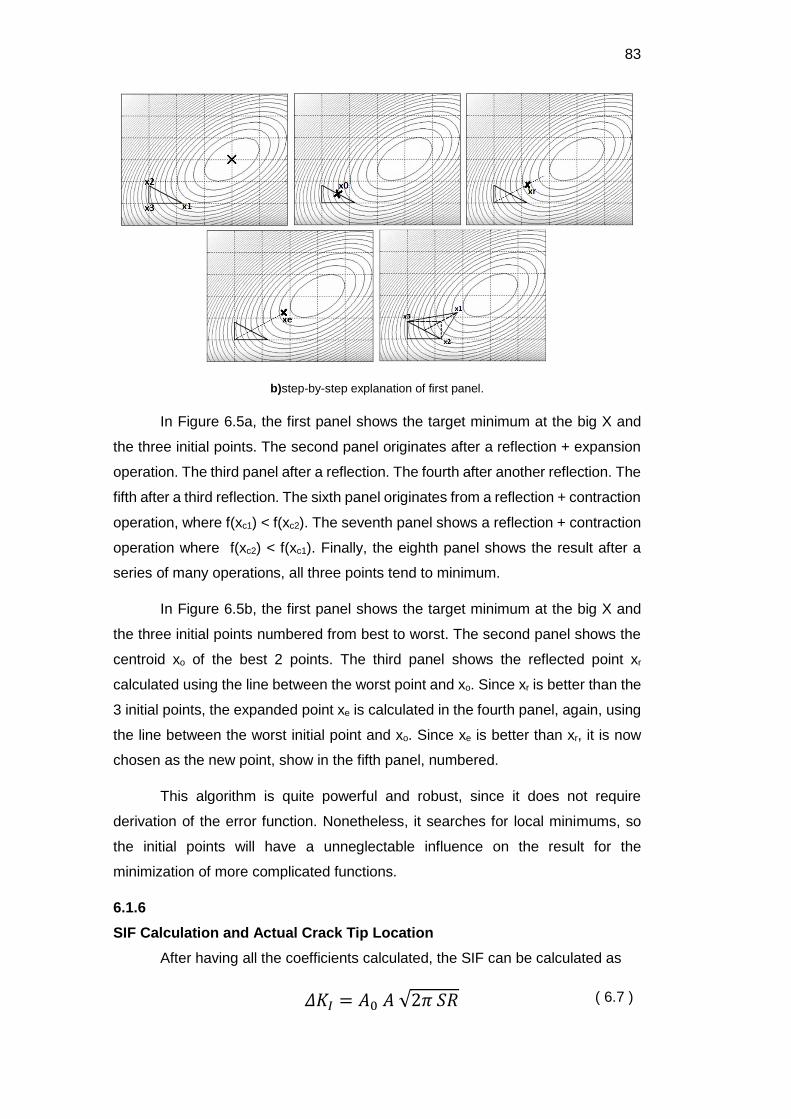
83
b)step-by-step explanation of first panel.
In Figure 6.5a, the first panel shows the target minimum at the big X and
the three initial points. The second panel originates after a reflection + expansion
operation. The third panel after a reflection. The fourth after another reflection. The
fifth after a third reflection. The sixth panel originates from a reflection + contraction
operation, where f(xc1) < f(xc2). The seventh panel shows a reflection + contraction
operation where f(xc2) < f(xc1). Finally, the eighth panel shows the result after a
series of many operations, all three points tend to minimum.
In Figure 6.5b, the first panel shows the target minimum at the big X and
the three initial points numbered from best to worst. The second panel shows the
centroid xo of the best 2 points. The third panel shows the reflected point xr
calculated using the line between the worst point and xo. Since xr is better than the
3 initial points, the expanded point xe is calculated in the fourth panel, again, using
the line between the worst initial point and xo. Since xe is better than xr, it is now
chosen as the new point, show in the fifth panel, numbered.
This algorithm is quite powerful and robust, since it does not require
derivation of the error function. Nonetheless, it searches for local minimums, so
the initial points will have a unneglectable influence on the result for the
minimization of more complicated functions.
6.1.6
SIF Calculation and Actual Crack Tip Location
After having all the coefficients calculated, the SIF can be calculated as
𝛥𝐾𝐼 = 𝐴0𝐴√2𝜋𝑆𝑅 ( 6.7 )
DBD
PUC-Rio - Certificação Digital Nº 1412756/CA

84
where ΔKI is the mode I SIF range in MPa√m, A0 is the first coefficient as described
in equation 6.2, A is the TSA calibration factor and SR is the spatial resolution.
In the non-linear approach, the values of xo and yo, as seen in equation 6.4,
are determined as well and the real location of the crack tip can be determined
𝑋𝑜 = 𝑋𝑜′ − 𝑥𝑜
𝑌𝑜 = 𝑌𝑜′ − 𝑦𝑜
( 6.8 )
where Xo and Yo give the calculated actual position of the crack tip.
6.2
Algorithm verification and Use
6.2.1
Numerically Generated TSA Data
Firstly, the algorithm is tested using an emulation of TSA data. Figure 6.6a
shows the numerically generated data and Figure 6.6b shows the fitted model for
the crack tip estimation at (-3,0) relatively to the actual position.
Figure 6.6: a)Numerically generated TSA data for crack tip at (-3,-1) and b)Calculated model for
estimated crack tip at (-3,0).
For the linear approach, where the crack tip location is not determined, the
final result of ΔKI was heavily dependent on the crack tip horizontal position
estimation (Xo’), presenting errors of 10% for just 1 pixel inaccuracy in the
estimation. For the vertical direction, the dependence was much smaller, a 1 pixel
inaccuracy in Yo’ resulted in an error of 0.4% for ΔKI.
The non-linear approach, on the other hand gave on-point results for ΔKI
even for crack-tip initial estimation coordinate (Xo’ and Yo’) errors of 20+ pixels in
the horizontal and vertical directions.
DBD
PUC-Rio - Certificação Digital Nº 1412756/CA

85
6.2.2
SIF Measurements
After this validation of the methodology, the algorithm was put to test on
several crack lengths (a) for the specimen shown in Figure 6.2a, Figure 6.3a and
Figure 6.4a.
The analyses were made using N=M=3, as described in equation 6.3, and
800 data points uniformly spaced between the Rmin and Rmax limiting circles. Figure
6.7 shows the selected data points for the specimen with a 14.1mm crack.
Table 6.1 shows the results for both the linear and non-linear approaches,
as well as for results determined with Digital Image Correlation (DIC) technique,
as developed by [79], and finite elements method (FEM) for the ΔKI as shown in
Appendix 5. Figure 6.8 shows the ΔKI/ΔP vs a plot. Caution was taken in order to
guarantee that the crack was completely opened, using high enough loads.
Figure 6.7: Selected data points for SIF calculation of a 14.1mm crack.
a
(mm)
ΔP
(N)
ΔKI/ΔP
TSA Linear
(10-3 MPa/N √m)
ΔKI/ΔP
TSA Non-linear
(10-3 MPa/N √m)
ΔKI/ΔP
DIC
(10-3 MPa/N √m)
ΔKI/ΔP
FEM
(10-3 MPa/N √m)
4.7 194 5.98 5.46 5.93 4.99 7.4 196 6.63 6.22 6.71 5.55 10 175 7.02
6.51 7.30 6.10 11.9 161 7.76 7.14 7.57 6.66 14.1 153 9.15 8.04 8.81 7.59 15.9 150 9.80 8.80 9.25 8.64 18.4 145 11.72 10.76 10.96 10.67 20.7 137 14.38 13.43 13.40 13.28
Table 6.1: Results for the SIF measurement using TSA, DIC and FEM.
DBD
PUC-Rio - Certificação Digital Nº 1412756/CA
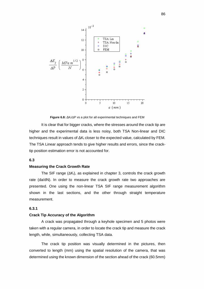
86
Figure 6.8: ΔKI/ΔP vs a plot for all experimental techniques and FEM
It is clear that for bigger cracks, where the stresses around the crack tip are
higher and the experimental data is less noisy, both TSA Non-linear and DIC
techniques result in values of ΔKI closer to the expected value, calculated by FEM.
The TSA Linear approach tends to give higher results and errors, since the crack-
tip position estimation error is not accounted for.
6.3
Measuring the Crack Growth Rate
The SIF range (ΔKI), as explained in chapter 3, controls the crack growth
rate (da/dN). In order to measure the crack growth rate two approaches are
presented. One using the non-linear TSA SIF range measurement algorithm
shown in the last sections, and the other through straight temperature
measurement.
6.3.1
Crack Tip Accuracy of the Algorithm
A crack was propagated through a keyhole specimen and 5 photos were
taken with a regular camera, in order to locate the crack tip and measure the crack
length, while, simultaneously, collecting TSA data.
The crack tip position was visually determined in the pictures, then
converted to length (mm) using the spatial resolution of the camera, that was
determined using the known dimension of the section ahead of the crack (60.5mm)
DBD
PUC-Rio - Certificação Digital Nº 1412756/CA

87
and its size in pixels in each picture. The non-linear algorithm was used to locate
the position in pixels, that was converted to length (mm) using the spatial resolution
of the infrared camera, determined in the same way.
The results are shown in Table 6.2 while Figure 6.9 shows the determined
(red) and measured (green) positions of the crack tip. The pixel values are
measured relative to the opposite border.
Measured
Crack Length
(mm)
Measured Crack
Tip position
(infrared Pixel)
Algorithm Crack
Tip Position
(infrared Pixel)
Algorithm
Crack Length
(mm)
Error
(mm)
4.5 261 265 3.7 0.7
8.3 268 273 7.3 1.0
11.1 278 281 10.5 0.6
13.0 292 293 12.8 0.2
14.4 311 313 14.0 0.4
Table 6.2: Results for crack tip position and crack length.
Figure 6.9: Determined by TSA (red) and measured with photos (green) cracks.
DBD
PUC-Rio - Certificação Digital Nº 1412756/CA

88
The results show that the algorithm can find the crack tip location with an
accuracy of about 1mm for smaller cracks, and that this error tends to diminish for
longer cracks9. Such decent measurements and knowledge of the number of
cycles between each crack length result makes da/dN values determination
possible, which could be plotted and fitted by Paris’ law.
6.3.2
da/dN Straight from Temperature Rise
The other approach to determine the crack growth rate involves measuring
the temperature in a way similar to what was done in chapter 5. That is, measuring
the temperature around the propagating crack and of a reference specimen,
simultaneously, and computing the difference between them (ΔT).
This method was discovered during an experiment that meant to investigate
crack propagation through a damage parameter like Φ (the Risitano’s material
property) as described in chapter 5.
During the propagation of another crack, the infrared camera made a video
by capturing 1 frame for each 4 seconds period. The resulting video shows the
crack propagating and the maximum ΔT rising, as expected. Since the load range
was kept constant, the stresses got higher with the increase in crack length, which
then causes a rise in temperature.
After the video was recorded, 11 points where the crack tip eventually
passed through were selected, Figure 6.10 shows these points before and after
the crack propagation.
Figure 6.10: Position of 11 points along the crack path.
9 The crack propagation front is not a straight line, it usually assumes a parabolic format. Photos of the cracks and fractures are show in Appendix 6.
DBD
PUC-Rio - Certificação Digital Nº 1412756/CA
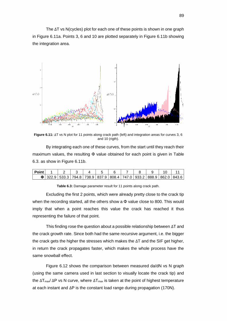
89
The ΔT vs N(cycles) plot for each one of these points is shown in one graph
in Figure 6.11a. Points 3, 6 and 10 are plotted separately in Figure 6.11b showing
the integration area.
Figure 6.11: ΔT vs N plot for 11 points along crack path (left) and integration areas for curves 3, 6
and 10 (rigth).
By integrating each one of these curves, from the start until they reach their
maximum values, the resulting Φ value obtained for each point is given in Table
6.3. as show in Figure 6.11b.
Point 1 2 3 4 5 6 7 8 9 10 11
Φ 322.9 533.3 794.8 738.9 837.9 808.4 747.0 933.2 888.9 862.0 843.6
Table 6.3: Damage parameter result for 11 points along crack path.
Excluding the first 2 points, which were already pretty close to the crack tip
when the recording started, all the others show a Φ value close to 800. This would
imply that when a point reaches this value the crack has reached it thus
representing the failure of that point.
This finding rose the question about a possible relationship between ΔT and
the crack growth rate. Since both had the same recursive argument, i.e. the bigger
the crack gets the higher the stresses which makes the ΔT and the SIF get higher,
in return the crack propagates faster, which makes the whole process have the
same snowball effect.
Figure 6.12 shows the comparison between measured da/dN vs N graph
(using the same camera used in last section to visually locate the crack tip) and
the ΔTmax/ ΔP vs N curve, where ΔTmax is taken at the point of highest temperature
at each instant and ΔP is the constant load range during propagation (170N).
DBD
PUC-Rio - Certificação Digital Nº 1412756/CA
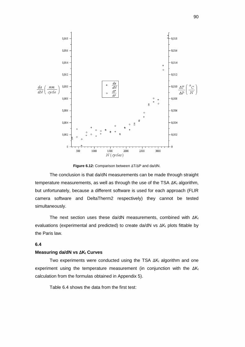
90
Figure 6.12: Comparison between ΔT/ΔP and da/dN.
The conclusion is that da/dN measurements can be made through straight
temperature measurements, as well as through the use of the TSA ΔKI algorithm,
but unfortunately, because a different software is used for each approach (FLIR
camera software and DeltaTherm2 respectively) they cannot be tested
simultaneously.
The next section uses these da/dN measurements, combined with ΔKI
evaluations (experimental and predicted) to create da/dN vs ΔKI plots fittable by
the Paris law.
6.4
Measuring da/dN vs ΔKI Curves
Two experiments were conducted using the TSA ΔKI algorithm and one
experiment using the temperature measurement (in conjunction with the ΔKI
calculation from the formulas obtained in Appendix 5).
Table 6.4 shows the data from the first test:
DBD
PUC-Rio - Certificação Digital Nº 1412756/CA
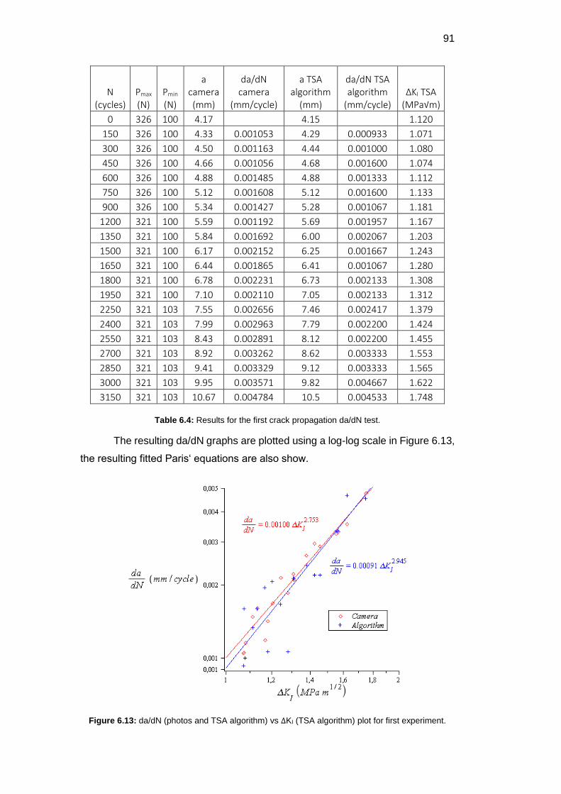
91
N (cycles)
Pmax (N)
Pmin (N)
a camera (mm)
da/dN camera
(mm/cycle)
a TSA algorithm
(mm)
da/dN TSA algorithm
(mm/cycle) ΔKI TSA (MPa√m)
0 326 100 4.17 4.15 1.120
150 326 100 4.33 0.001053 4.29 0.000933 1.071
300 326 100 4.50 0.001163 4.44 0.001000 1.080
450 326 100 4.66 0.001056 4.68 0.001600 1.074
600 326 100 4.88 0.001485 4.88 0.001333 1.112
750 326 100 5.12 0.001608 5.12 0.001600 1.133
900 326 100 5.34 0.001427 5.28 0.001067 1.181
1200 321 100 5.59 0.001192 5.69 0.001957 1.167
1350 321 100 5.84 0.001692 6.00 0.002067 1.203
1500 321 100 6.17 0.002152 6.25 0.001667 1.243
1650 321 100 6.44 0.001865 6.41 0.001067 1.280
1800 321 100 6.78 0.002231 6.73 0.002133 1.308
1950 321 100 7.10 0.002110 7.05 0.002133 1.312
2250 321 103 7.55 0.002656 7.46 0.002417 1.379
2400 321 103 7.99 0.002963 7.79 0.002200 1.424
2550 321 103 8.43 0.002891 8.12 0.002200 1.455
2700 321 103 8.92 0.003262 8.62 0.003333 1.553
2850 321 103 9.41 0.003329 9.12 0.003333 1.565
3000 321 103 9.95 0.003571 9.82 0.004667 1.622
3150 321 103 10.67 0.004784 10.5 0.004533 1.748
Table 6.4: Results for the first crack propagation da/dN test.
The resulting da/dN graphs are plotted using a log-log scale in Figure 6.13,
the resulting fitted Paris‘ equations are also show.
Figure 6.13: da/dN (photos and TSA algorithm) vs ΔKI (TSA algorithm) plot for first experiment.
DBD
PUC-Rio - Certificação Digital Nº 1412756/CA

92
They show good agreement, showing that TSA can single-handedly
measure a da/dN curve.
The second experiment compared the results obtained by the TSA
algorithm and FEM for the ΔKI while the da/dN was measured using the camera
method. Again, the data is listed in Table 6.5.
The objective this time was to investigate if crack closure was affecting the
measurement. In order to do that, the minimum load (and the maximum load, for
reasons described in chapter 4) was lowered. Doing this permits the crack to close,
and should make the effective ΔK different from the one predicted by FEM.
Figure 6.14 shows the da/dN vs ΔKI plots for the TSA algorithm and FEM
results. If left untouched (ΔKI TSA 1), the algorithm finds values of ΔKI
systematically lower than the ones predicted by FEM. On the other hand, if special
care is taken so that the algorithm uses only data far enough (twice the value of
Rmin) from the crack tip (ΔKI TSA 2), the results are almost identical.
N (cycles)
Pmax (N)
Pmin (N)
a (mm)
da/dN (mm/cycle)
ΔKI TSA1 (MPa√m)
ΔKI FEM (MPa√m)
ΔKI TSA2 (MPa√m)
15051 223 61 10.4 0.000302 0.940 1.004 1.05
20211 221 62 12.5 0.000407 1.030 1.093 1.165
24930 222 65 14.5 0.000424 1.110 1.224 1.268
28798 222 63 16.6 0.000603 1.260 1.416 1.421
30695 223 58 18.6 0.001054 1.364 1.652 1.679
31907 222 58 20.6 0.00165 1.678 1.959 1.958
32464 223 63 22.6 0.003591 1.881 2.353 2.384
32830 218 65 24.6 0.005464 2.068 2.813 2.783
32980 216 60 26.6 0.013333 2.790 3.435 3.522
Table 6.5: Results for the second crack propagation da/dN test.
These results suggest that the TSA algorithm is actually measuring the
effective SIF. Since the values found were lower than the predicted ones, part of
the applied load is supposedly being used to open the crack. Nonetheless, taking
data points far from the crack tip seem to nullify this effect.
DBD
PUC-Rio - Certificação Digital Nº 1412756/CA
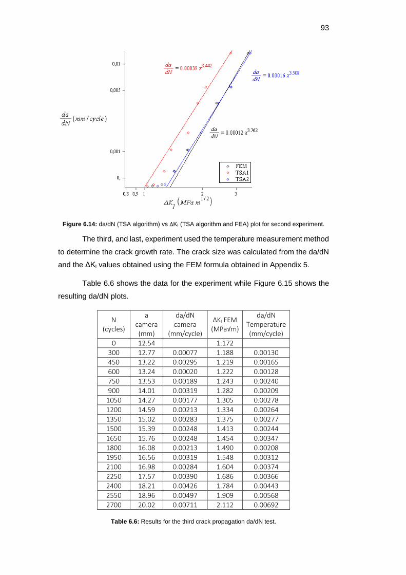
93
Figure 6.14: da/dN (TSA algorithm) vs ΔKI (TSA algorithm and FEA) plot for second experiment.
The third, and last, experiment used the temperature measurement method
to determine the crack growth rate. The crack size was calculated from the da/dN
and the ΔKI values obtained using the FEM formula obtained in Appendix 5.
Table 6.6 shows the data for the experiment while Figure 6.15 shows the
resulting da/dN plots.
N (cycles)
a camera (mm)
da/dN camera
(mm/cycle)
ΔKI FEM (MPa√m)
da/dN Temperature (mm/cycle)
0 12.54 1.172
300 12.77 0.00077 1.188 0.00130
450 13.22 0.00295 1.219 0.00165
600 13.24 0.00020 1.222 0.00128
750 13.53 0.00189 1.243 0.00240
900 14.01 0.00319 1.282 0.00209
1050 14.27 0.00177 1.305 0.00278
1200 14.59 0.00213 1.334 0.00264
1350 15.02 0.00283 1.375 0.00277
1500 15.39 0.00248 1.413 0.00244
1650 15.76 0.00248 1.454 0.00347
1800 16.08 0.00213 1.490 0.00208
1950 16.56 0.00319 1.548 0.00312
2100 16.98 0.00284 1.604 0.00374
2250 17.57 0.00390 1.686 0.00366
2400 18.21 0.00426 1.784 0.00443
2550 18.96 0.00497 1.909 0.00568
2700 20.02 0.00711 2.112 0.00692
Table 6.6: Results for the third crack propagation da/dN test.
DBD
PUC-Rio - Certificação Digital Nº 1412756/CA

94
Figure 6.15: da/dN (temperature and photos) vs ΔKI (FEA) plot for third experiment.
Again, the results show good agreement, proving the validity of both
methods for measuring the crack growth rate.
Finally, all results are plotted, together with reference results described in
chapter 3, in one single graph in Figure 6.16.
Figure 6.16: Plot of all da/dN results and references.
DBD
PUC-Rio - Certificação Digital Nº 1412756/CA

95
Reasonable agreement is seen throughout all results and between them
and the references. Nonetheless, the observed differences are attributed to the
lack of mean load control, for reasons explained in chapter 4, and to variations in
the test temperature between 20ºC and almost 40ºC, since, during summer in Rio
the temperature can get really high. As shown by many authors and discussed in
chapter 3, these variations can cause changes in both the slope and intercept of
the Paris curve.
DBD
PUC-Rio - Certificação Digital Nº 1412756/CA
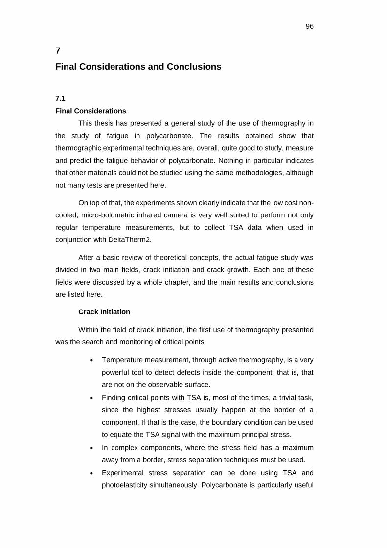
96
7
Final Considerations and Conclusions
7.1
Final Considerations
This thesis has presented a general study of the use of thermography in
the study of fatigue in polycarbonate. The results obtained show that
thermographic experimental techniques are, overall, quite good to study, measure
and predict the fatigue behavior of polycarbonate. Nothing in particular indicates
that other materials could not be studied using the same methodologies, although
not many tests are presented here.
On top of that, the experiments shown clearly indicate that the low cost non-
cooled, micro-bolometric infrared camera is very well suited to perform not only
regular temperature measurements, but to collect TSA data when used in
conjunction with DeltaTherm2.
After a basic review of theoretical concepts, the actual fatigue study was
divided in two main fields, crack initiation and crack growth. Each one of these
fields were discussed by a whole chapter, and the main results and conclusions
are listed here.
Crack Initiation
Within the field of crack initiation, the first use of thermography presented
was the search and monitoring of critical points.
Temperature measurement, through active thermography, is a very
powerful tool to detect defects inside the component, that is, that
are not on the observable surface.
Finding critical points with TSA is, most of the times, a trivial task,
since the highest stresses usually happen at the border of a
component. If that is the case, the boundary condition can be used
to equate the TSA signal with the maximum principal stress.
In complex components, where the stress field has a maximum
away from a border, stress separation techniques must be used.
Experimental stress separation can be done using TSA and
photoelasticity simultaneously. Polycarbonate is particularly useful
DBD
PUC-Rio - Certificação Digital Nº 1412756/CA

97
in this approach, since it can be used as a coating for both
techniques.
Analytical stress functions are often used as a way to numerically
separate the stresses in what is called a hybrid TSA technique.
Then, the stress concentration problem is attacked using TSA.
The stress concentration factor of a SAE keyhole specimen is
experimentally determined using TSA. Two approaches were used,
a simpler one, that utilize the boundary condition argument, and a
more complex one that used the stress function approach.
The simpler method used a simple equation to extrapolate the
experimental data, and achieved acceptable results for Kt by doing
so.
The second method separated the principal stresses using a Airy’s
stress function approach. The whole stress field was determined for
all components. Again, the results obtained were good.
The TSA results were compared to DIC, photoelasticity and FEM
results. All of them shown good agreement with the literature
predicted value.
After the stresses acting on the specimen have been fully determined, the
actual fatigue properties are determined with the use of thermography.
The fatigue limit of polycarbonate is measured through the
thermographic method (Risitano’s method), which is based on an
energy approach to fatigue damage.
The material presents different thermal behavior when cyclically
loaded below and above a certain stress level. This stress level is
supposed to be the fatigue limit.
The results obtained using this method are similar to those found on
the literature for polycarbonate, although they fell on the high end of
the range, which was not expected.
More test could be done to make a better estimation of the fatigue
limit.
Later, an experiment had a specimen failing by fatigue under
loading range lower than what was measured as the fatigue limit.
The next, and final, step of the crack initiation study is to determine the SN
curve of the material.
DBD
PUC-Rio - Certificação Digital Nº 1412756/CA

98
The thermographic method is once again used to accomplish this
task. Based on the same energy approach to fatigue damage.
This time, a parameter Φ is used as a material property, which
indicates that a critical damage level has been reached and failure
is eminent.
With this approach, the fatigue curve is, theoretically, measured
using a single specimen, in a very short time.
The results found show good agreement with the literature curves
for polycarbonate, although some variables could not be controlled
or compared.
Parameters such as the mean stress, frequency and thickness
effect were all constant throughout the study.
Crack Growth
After a crack has initiated in a component, the study of its propagation under
cyclic loading is presented. Thermography once again is used, and the first step is
to apply TSA to fracture mechanics.
An algorithm was developed to measure mode I stress intensity
factors using TSA and Westergaard’s stress function for the stress
field near the tip of a fatigue crack. Two approaches were used, a
linear and a non-linear one.
The algorithm has a routine to make an initial crack tip position
estimation. This estimation is needed in both approaches.
The linear approach is very sensitive to initial crack tip location
estimation while the non-linear approach uses the crack tip position
as an adjustable variable, resulting in a powerful tool for finding the
actual tip of the crack.
The algorithm selects data points to be fitted using a linearity
argument, which certifies that the points can be modelled by the
Westergaard‘s equations.
The results obtained for ΔKI were verified using simulated TSA data,
FEM analysis, as well as other experimental technique (DIC).
The results shown very good agreement with the predicted and
measured values.
DBD
PUC-Rio - Certificação Digital Nº 1412756/CA

99
The next step on the way to determining the crack growth behavior of
polycarbonate was to measure crack growth rates. Once again, thermography was
used to accomplish the task.
Two approaches were used to measured crack growth rate. The first
used the non-linear SIF measurement algorithm, while the second
used temperature measurements.
When using the algorithm to follow the crack tip throughout its
propagation, the results were very good. The reference
measurements were made using a regular digital camera, which
took photos simultaneously to the TSA data collection, and posterior
visual determination of the crack tip position.
The second method was found during tests that explored a possible
damage approach to fatigue crack propagation, based on the
parameter proposed by Risitano.
The findings show that the rise in temperature provoked by the
fatigue damage is proportional to the crack growth rate.
Both approaches had great results, and could locate the actual
crack tip location with high accuracy.
Finally, the crack growth rate vs SIF curves could be measured.
Three tests were conducted, two of them used the algorithm and
the third used the temperature method combined with the FEM
result.
The results obtained for all tests showed good agreement between
themselves and in comparison to literature results.
The effect of crack closure was observed in the second test, which
demonstrated that the algorithm measures the effective SIF range
through TSA data.
Eventual variations on the results are attributed to mean stress
and temperature differences.
Overall, the results were good, highlighting the power of thermography as
a tool for fatigue studies. On top of that, the inexpensive setup used in this work
proved to be just as reliable for this type of studies as the more common, more
expensive equipment.
DBD
PUC-Rio - Certificação Digital Nº 1412756/CA

100
7.2
Conclusions
For fatigue crack initiation, the thermographic method produced great
results when it comes to fatigue limit and fatigue curve measurements. The
greatest feature of the method is the capability to reduce the time needed for such
tests to a fraction of the traditional methods.
In the study of fatigue crack growth, thermographic stress analysis,
combined with numerical approaches, was proven to be particularly useful, both in
measuring stress concentrations and stress intensity factors. With some tweaking,
the algorithms presented could be used to make these measurements in real time.
Special attention is draw to two points: the possibilities opened by the
thermographic approach to fatigue damage, i.e. a point-by-point evaluation of the
Φ integral during fatigue crack propagation, and to the relationship between the
crack propagation rate and the temperature change ahead of the crack (See Figure
6.12 on page 86).
Overall, infrared thermography is a great tool for fatigue studies and,
through temperature measurements, permits the observation of a somewhat
unexplored aspect of the problem, from which new models as well as new testing
routines can be devised.
DBD
PUC-Rio - Certificação Digital Nº 1412756/CA

101
8
Bibliography
[1]W. Herschel, “Experiments on the refrangibility of the visible rays of the sun”,
Philosophical Transactions of the Royal Society of London, vol. 90, pp. 284–292, 1800.
[2]Flir, “The ultimate infrared handbook for R&D professionals”. FLIR AB, Boston.
Available for free at www.flir.com.
[3]M. Razeghi, “Current status and future trends of infrared detectors”, Opto-
Electronics Review, vol. 6, no. 3, pp. 155–194, 1998.
[4]S. P. Langley, “The bolometer”, in Vallegheny Observatory, The Society Gregory,
New York, NY, USA, 1880.
[5]Corsi, Carlo. “Infrared A Key Technology for Security Systems”, Advances in
Optical Technologies, 2012 (2012) 1-15.
[6]Overstreet R., “Notes on using Microbolometers at hogh frame rates”, FLIR
systems, April 2013, Rev3.
[7]Ibarra-Castanedo C. “Quantitative Subsurface Defect Evaluation by Pulsed Phase
Thermography: Depth Retrieval with the Phase” PhD thesis, Universite Laval, 2005.
[8]K. Chatterjee, S. Tuli, S. Pickering, and D. Almond. “A comparison of the pulsed,
lock-in and frequency modulated thermography nondestructive evaluation
techniques” NDT&E International, 44:655–667, 2011.
[9]Y.Y. Hung, Y.S. Chen, S.P. Ng, L. Liu, Y.H. Huang, B.L. Luk, R.W.L. Ip, C.M.L. Wu
and P.S. Chung. “Review and comparison of sherography and active thermography
for nondestructive evaluation” Materials Science and Engineering R., 64:73–112,
2009.
[10]Sun, J.G., “Analysis of pulsed thermography methods for defect depth
prediction” Journal of Heat Transfer, 128, p. 329-338, 2006.
[11]Avdelidis, N.P., Ibarra-Castanedo, C., Maldague, X., Marioli-Riga, N.P., and Almond,
D.P., “A thermographic comparison study for the assessment of composite
patches” Infrared Physics and Technology, 45: p. 291-299, 2004.
[12]Maldague X. P. V., Jones T. S., Kaplan H., Marinetti S. and Prystay M. "Chapter 2:
Fundamentals of Infrared and Thermal Testing: Part 1. Principles of Infrared and
Thermal Testing" in Nondestructive Handbook, Infrared and Thermal Testing, Volume
DBD
PUC-Rio - Certificação Digital Nº 1412756/CA

102
3, X. Maldague technical ed., P. O. Moore ed., 3rd edition, Columbus, Ohio, ASNT Press,
2001.
[13]Thomson, W. (Lord Kelvin), "On the Dynamical Theory of Heat", Transaction of the
Royal Society of Edinbourgh, vol.20, pp. 261-283, 1853.
[14]Barber J. R., “Elasticity”, Solid Mechanics and its Applications Vol. 172, Chapter 14,
p. 219-225, 2010.
[15] Dulieu-Barton, J.M., "Introduction to thermoelastic stress analysis", Strain, pp.
35-39, May, 1999.
[16]Dulieu-Smith, S.M., "Alternative calibration techniques for quantitative
thermoelastic stress analysis", Strain , pp. 9-16, February, 1995.
[17]Freire J.L.F., Waugh R.C., Fruehmann R., Dulieu-Barton J.M., “Using
Thermoelastic Stress Analysis to Detect Damaged and Hot Spot Areas in
Structural Components”, In: Proc. Of the XXXII Congresso Nacional de Ensaios Não
Destrutivos e Inspeção (CONAEND), São Paulo, ABENDI, 2014.
[18]Stress Photonics Inc., “DeltaTherm 2 Manual“, v6, January, 2016.
[19]Khaja A.A., Rowlands R.E., “Experimentally determined stresses at geometric
discontinuities using simple stress functions”, Journal of Engineering Mechanics,
Vol. 141, 11, 2015.
[20]Kurunthottikkal Philip S., Rowlands R.E., “Hybrid full-field stress analysis of
loaded perforated asymmetrical plate”, Proceedings of the 2015 Annual Conference
on Experimental and Applied Mechanics, Vol.9, pp. 235-241, 2016.
[21]Samad W.A., Rowlands R.E., “On improving thermoelastic stress analysis data
near edges of discontinuities”, Proceedings of the 2014 Annual Conference on
Experimental and Applied Mechanics, Vol. 6, pp. 157-162, 2015.
[22]Lin S.J., Samad W.A., Khaja A.A., Rowlands R.E., “Hybrid thermoelastic stress
analysis”, Experimental Mechanics, 55, pp. 653-665, 2015.
[23]Barone, S., Patterson, E.A., "Full-field separation of principal stresses by
combined Thermo- and Photoelasticity", Experimental Mechanics, Vol. 36 (4), pp.
318-324, 1996.
[24]Barone, S., Patterson, E. A., "The development of simultaneous thermo- and
photo-elasticity for principal stress analyses", Strain, pp. 57-65, May 1999.
[25]Wang W., Fruehmann R.K., Dulieu-Barton J.M., “Application of Digital Image
Correlation to address complex motions in thermoelastic stress analysis”, Strain,
Vol. 51 (5), pp. 405-418, October 2015.
DBD
PUC-Rio - Certificação Digital Nº 1412756/CA

103
[26]Silva M.L., Ravichandran G., “Combined thermoelastic stress analysis and
digital image correlation with a single infrared camera”, The Journal of Strain
Analysis for Engineering Design, Vol. 46 (8), pp. 783-793, November 2011.
[27]Machin A.S., Sparrow J.G., Stimson M.G., “Mean stress dependence of the
thermoelastic constant”, Strain, pp. 27-30, February 1987.
[28] Dunn, S., Lombardo, D., Sparrow, J.G., "The mean stress effect in metallic alloys
and composites", Proceedings of the International Conference on Stress and Vibration
(Including 3rd Int.Conf. on Stress Analysis by Thermoelastic techniques), London, SPIE
vol. 1084, pp. 129-142, 1989.
[29]Wong, A.K., Dunn, S.A., Sparrow, J.G., "Residual stress measurement by means
of the thermoelastic effect", Nature, vol. 332, No. 6165, pp. 613-615, April 1988.
[30]Quinn S., Dulieu-Barton J.M., Eaton-Evans J., Fruehmann R.K., Tatum P.J.
“Thermoelastic assessment of plastic deformation“, The Journal of Strain Analysis
for Engineering Design, Vol. 43 (6), pp. 451-468, 2008.
[31]Jones, R., Heller, M., Lombardo, D., Dunn, S, Paul, J., Saunders, D., "Thermoelastic
assessment of damage growth in composites", Composite Structures, 12, pp. 291-
314, 1989.
[32]Zhang, D., Sandor, B.I., "A thermoelastic theory for damage in anisotropic
materials", Fatigue and Fracture of Engineering Materials and Structures, 13, pp. 497-
509, 1990. [33]Dulieu-Smith, J.M., Stanley, P., "A review of damage studies in fiber reinforced
composites using the thermoelastic technique", XXV AIAS National Conference &Int.
Conf. On Material Engineering, Lecce, pp. 891-898, 1996.
[34]Tomlinson R.A., Olden E.J., “Thermoelasticity for the analysis of crack tip stress
fields – A review“, Strain, Vol. 35 (2), pp. 49-55, 1999.
[35]Tomlinson R.A., Nurse A.D., Patterson E.A, “On determining stress intensity
factors for mixed-mode cracks from thermoelastic data”, Fatigue and Fracture of
Engineering Materials and Structures, Vol. 20 (2), pp. 217-226, 1997.
[36]Dulieu-Barton J.M., Fulton M.C., Stanley P., “The analysis of thermoelastic
isopachic data from crack tip stress fields”, Fatigue and Fracture of Engineering
Materials and Structures, Vol. 23, pp. 301-313, 2000.
[37]Lin S.T., Feng Z., Rowlands R.E., “Thermoelastic determination of stress
intensity factors in orthotropic composites using the J-integral”, Engineering
Fracture Mechanics, Vol. 56 (4), pp. 579-592, 1997.
[38]Diaz F.A., Patterson E.A., Tomlinson R.A., Yates J.R., “Measuring stress intensity
factors during fatigue crack growth using thermoelasticity”, Fatigue and Fracture of
Engineering Materials and Structures, Vol. 27 (7), pp. 571-583, 2004.
DBD
PUC-Rio - Certificação Digital Nº 1412756/CA

104
[39]Tomlinson R.A., Du Y., Patterson E.A., "Understanding Crack Tip Plasticity – a
Multi-Experimental Approach", Applied Mechanics and Materials, Vol. 70, pp. 153-
158, 2011.
[40]Marsavina L., Tomlinson R.A., Patterson E.A., Yates J.R., “Investigation of Crack
Closure by Using Thermoelastic Stress Analysis“, Proceedings of the 16th European
Conference of Fracture, Alexandroupolis, Greece, pp. 443-444, July 2006.
[41]Patki A.S., Patterson E.A., “Thermoelastic stress analysis of fatigue cracks
subject to overloads”, Fatigue and Fracture of Engineering Materials and Structures,
Vol. 33 (12), pp. 809-821, 2010.
[42]Tomlinson R.A., Marsavina L., “Thermoelastic investigations for fatigue life
assessment”, Experimental Mechanics, Vol. 44 (5), pp. 487-494, 2004.
[43]Yates J.R., Zanganeh M. Tomlinson R.A., Brown M.W. Diaz Garrido F.A., “Crack
paths under mixed mode loading”, Engineering Fracture Mechanics, Vol. 75 (3-4), pp.
319-330, 2008.
[44]CASTRO, J. T. P. D.; MEGGIOLARO, M. A.: “Fadiga – Técnicas e Práticas de
Dimensionamento Estrutural sob Cargas Reais de Serviço. Volume I – Iniciação de
Trincas.” CreateSpace, 2009.
[45]Vieira R.B., Philip S.K., Gonzáles G.L.G, Freire J.L.F., Yang B., Rowlands R.E.
“Determination of a U-notch aluminum plate stress concentration factor by
thermoelasticity”, In: Proc. Of the 13th Conferência sobre Tecnologia de Equipamentos,
Recife, ABENDI, 2015.
[46]Vieira R.B., Freire J.L.F., “Using Visual Techniques (TSA, DIC and
Photoelasticity) to Determine Stress Concentration Factors”, In: Proc. Of the 17th
International Conference on Experimental Mechanics, Rhodes, July 3-7, 2016.
[47]Yang M., Pizhing Q., “Generalized fatigue model for polymer matrix
composites”, In: Proc. Of the International Conference on Computational &
Experimental Engineering and Sciences, Vol. 6 (3), pp.157-168, 2008.
[48]CASTRO, J. T. P. D.; MEGGIOLARO, M. A.: “Fadiga – Técnicas e Práticas de
Dimensionamento Estrutural sob Cargas Reais de Serviço. Volume II – Propagação de
Trincas, Efeitos Térmicos e Estocásticos.” CreateSpace, 2009.
[49]“Overview of materials for Polycarbonate, Extruded”, Available in:
http://www.matweb.com/search/DataSheet.aspx?MatGUID=501acbb63cbc4f748faa74
90884cdbca, accessed on: 02/09/2016.
[50]Crawford R.J., “Plastics Engineering”, 2nd edition, New York, Pergamon Press,
1990.
[51]Hertzberg R.W., Nordberg H., Manson J.A., “Fatigue Crack Propagation in
Polymeric Materials”, Journal of Materials Science, Vol. 5, pp. 521-526, 1970.
DBD
PUC-Rio - Certificação Digital Nº 1412756/CA
105
[52]Martin G.C., Gerberich W.W., “Temperature effects on fatigue crack growth in
polycarbonate”, Journal of Materials Science, Vol. 11, pp. 231-238, 1976.
[53]Hertzberg R.W., Manson J.A., “Fatigue of Engineering Plastics”, New York,
Academic Press, 1980.
[54]Pitman G., Ward I.M., “The molecular weight dependence of fatigue crack
propagation in polycarbonate“, Journal of Materials Science, Vol. 15, pp. 635-645,
1980.
[55]Pruitt L., Rondinone D., “The effect of specimen thickness and stress ratio on
the fatigue behavior of polycarbonate”, Polymer Engineering and Science, Vol. 36 (9),
pp.1300-1305, 1996.
[56]Haddaoui N., Chudnovsky A., Moet A., “Ductile fatigue crack propagation in
polycarbonate”, Polymer, Vol. 27, pp. 1377-1384, 1986.
[57]James M.N., Christopher C.J., Lu Y., Patterson E.A.,“Fatigue crack growth and
craze induced crack tip shielding in polycarbonate”,Polymer, Vol. 53, pp.1558-1570,
2012.
[58]Chen T.J., Bosnyak C.P., Kao C.I., Chudnovsky A.,“A fatigue crack initiation map
for polycarbonate”,Journal of Applied Pol. Science, Vol. 49 (11), pp1909-1919, 1993.
[59]Chen T.J., Chudnovsky A., Bosnyak C.P., “Observations of the micro-
mechanisms of fatigue-crack initiation in polycarbonate”, Journal of Materials
Science, Vol. 29 (22), pp 5903-5910, 1994.
[60]Mackay M.E., Teng T.G., Schultz J.M., “Craze roles in the fatigue of
polycarbonate”, Journal of Materials Science, Vol. 14, pp. 221-227, 1979.
[61]Wang B., Lu H., Tan G., Chen W., “Strength of damaged polycarbonate after
fatigue”, Theoretical and Applied Fracture Mechanics, Vol. 39, pp. 163-168, 2003.
[62]Jansen R.P.M., Kanter D., Govaert L.E., Meijer H.E.H., “Fatigue Life Predictions
for Glassy Polymers: A Constitutive Approach”, Macromolecules, Vol. 41, pp.2520-
2530, 2008.
[63]Kim G.H., Lu H., “Accelerated fatigue life testing of polycarbonate at low
frequency under isothermal condition”, Polymer Testing, Vol. 27, pp. 114-121, 2008.
[64] “SAE Keyhole Test Program”, Available in:
https://www.efatigue.com/benchmarks/SAE_keyhole/SAE_keyhole.html, accessed on:
10/09/2016.
[65]Measurements Group Inc., “Instructions for machining two-dimensional models
from PSM-1”, Instruction Bulletin IB-201, Raleigh, USA, 1974.
[66]Alva J.G.C., “Controle por aprendizado neuro-fuzzy aplicado a uma máquina de
fadiga atuada por um músculo pneumático”, PhD Thesis, Pontifícia Universidade
Católica do Rio de Janeiro, Departamento de Engenharia Mecânica, 2013.
DBD
PUC-Rio - Certificação Digital Nº 1412756/CA
106
[67]Shukla A., Dally J.W., “Experimental Solid Mechanics”, College Enterprises, 2010.
[68]La Rosa G., Risitano A., “Thermographic methodology for rapid determination
of the fatigue limit of materials and mechanical components”, International Journal
of Fatigue, Vol. 22, pp. 65-73, 2000.
[69]Fargione G., Geraci A., La Rosa G., Risitano A., “Rapid determination of the
fatigue curve by the thermographic method”, International Journal of Fatigue, Vol. 24,
pp. 11-19, 2002.
[70]Plastifab Inc., “Polycarbonate Tube Data Sheet”, Available in:
http://www.plastifab.ca/a-upload-pdfs/4_02.pdf, accessed on: 16/09/2016.
[71]“Typical properties of polycarbonates (PC)”, Available in:
http://www.nationwideplastics.net/pdfs/Polycarbonate/(New)%20Polycarbonate%20Mat
erial%20Datasheet.pdf, accessedoin: 16/09/2016.
[72]McKeen L.W., “Fatigue & Tribological Properties of Plastics & Elastomers”, 2nd
edition, William Andrew, 2009.
[73]Stanley P., Chan W. K., “The determination of stress intensity factors and crack
tip velocities from thermoelastic infra-red emissions”, In: Proceedings of
International Conference of Fatigue of Engineering Materials and Structures, c262,
IMechE, Sheffield, UK, pp. 105–114, 1986.
[74]Stanley P., Dulieu-Smith J. M., “Progress in the thermoelastic evaluation of
mixed mode stress intensity factors”, In: Proceedings of the SEM Spring Conference
on Experimental Mechanics, Dearborn, pp. 617–626, 1993.
[75]Lesniak J. R., Bazile D. J., Boyce B. R., Zickel M. J., Cramer K. E., Welch, C. S.,
“Stress intensity measurement via infrared focal plane array”, Non-Traditional
Methods of Sensing Stress, Strain, and Damage in Materials and Structures. ASTM STP
1318, Philadelphia, 1997.
[76]Díaz F. A., Yates J. R., Tomlinson R. A., Patterson E. A., “Some observation on
the application of thermoelasticity to fatigue cracks”, In: Proceedings of SEM
Conference, Milwaukee, USA, 2002.
[77]Díaz F. A., Patterson E. A., Tomlinson R. A., Yates J. R., “Measuring stress
intensity factors during fatigue crack growth using thermoelasticity”, Fatigue and
Fracture of Engineering Materials and Structures, Vol. 27, pp. 571-583, 2004.
[78]Nelder J. A., Mead R., “A simplex method for function minimization”, The
Computer Journal, Vol. 7, pp. 308–313, 1965.
[79]Gonzáles G. L. G., Díaz J. G., Gonzáles J. A. O., Castro J. T. P., Freire J. L. F.,
“Determining SIFs Using DIC Considering Crack Closure and Blunting”, In:
Proceedings of the SEM Annual Conference on Experimental Mechanics, Orlando,
Jun. 6-9, 2016.
DBD
PUC-Rio - Certificação Digital Nº 1412756/CA

107
Appendix 1 Simple Test on Defect Location by Active Thermography
In order to demonstrate the power of active thermography in detecting defects,
this appendix describes two simple experiments.
The specimens consisted of a rectangular bar of a glass-fiber composite with
polymeric matrix and a rectangular bar of steel. Both had holes drilled into them as shown
by Figure A1.1.
Figure A1.1: a)Composite and b)steel specimens for defect detection experiment.
The composite specimen had three holes drilled from its back up to ¼, ½ (1) and
¾ (2) of its thickness. The ¼ hole could not be detected, hence why it is not identified
neither with an arrow neither by a number. Another passing hole (3) was drilled through
its width with the center at a ½ thickness depth.
The steel specimen had two holes drilled through its width up to about half the
way , one (1) with its center at a ½ thickness depth and the other (2) with its center at ¼
thickness depth.
The experimental procedure consisted of pointing the infrared camera at the
specimens and applying heat to the front surface using a commercial hair dryer (2000W),
then, the difference in temperature decay can be seen.
For the composite specimen, because of its thermal properties (good insulator /
bad conductor) the heat was applied for a relatively long period (15-20 seconds) and
DBD
PUC-Rio - Certificação Digital Nº 1412756/CA
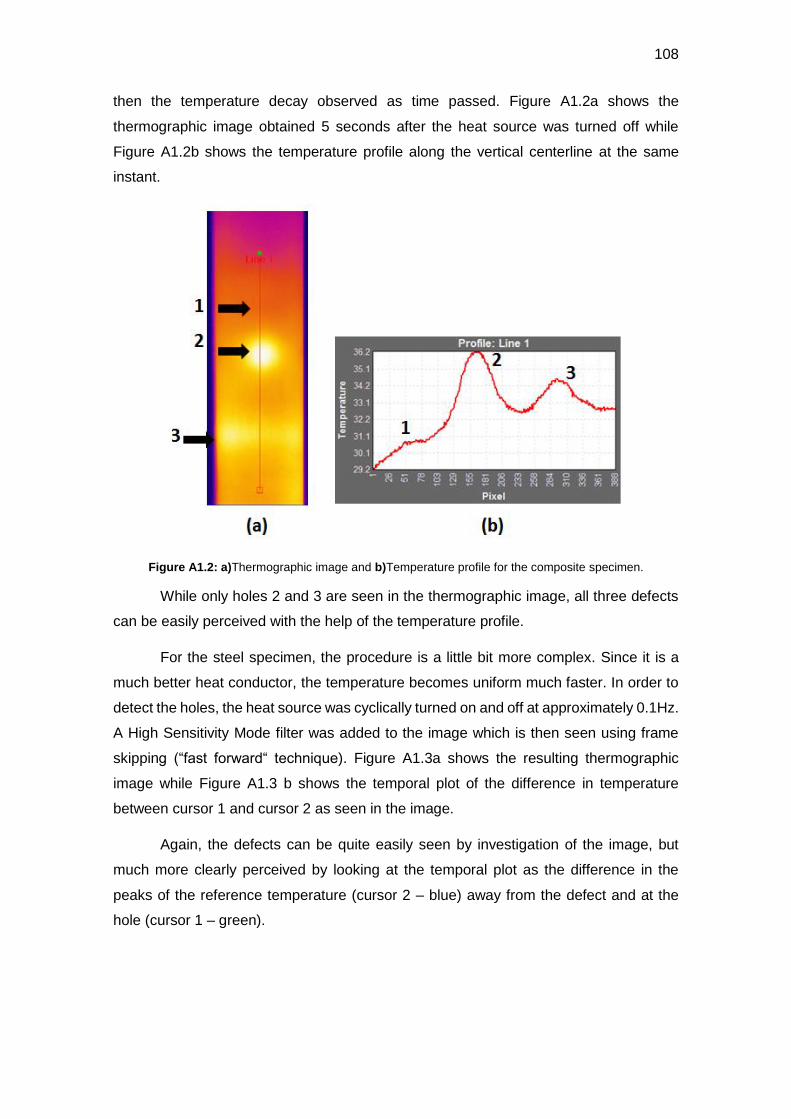
108
then the temperature decay observed as time passed. Figure A1.2a shows the
thermographic image obtained 5 seconds after the heat source was turned off while
Figure A1.2b shows the temperature profile along the vertical centerline at the same
instant.
Figure A1.2: a)Thermographic image and b)Temperature profile for the composite specimen.
While only holes 2 and 3 are seen in the thermographic image, all three defects
can be easily perceived with the help of the temperature profile.
For the steel specimen, the procedure is a little bit more complex. Since it is a
much better heat conductor, the temperature becomes uniform much faster. In order to
detect the holes, the heat source was cyclically turned on and off at approximately 0.1Hz.
A High Sensitivity Mode filter was added to the image which is then seen using frame
skipping (“fast forward“ technique). Figure A1.3a shows the resulting thermographic
image while Figure A1.3 b shows the temporal plot of the difference in temperature
between cursor 1 and cursor 2 as seen in the image.
Again, the defects can be quite easily seen by investigation of the image, but
much more clearly perceived by looking at the temporal plot as the difference in the
peaks of the reference temperature (cursor 2 – blue) away from the defect and at the
hole (cursor 1 – green).
DBD
PUC-Rio - Certificação Digital Nº 1412756/CA
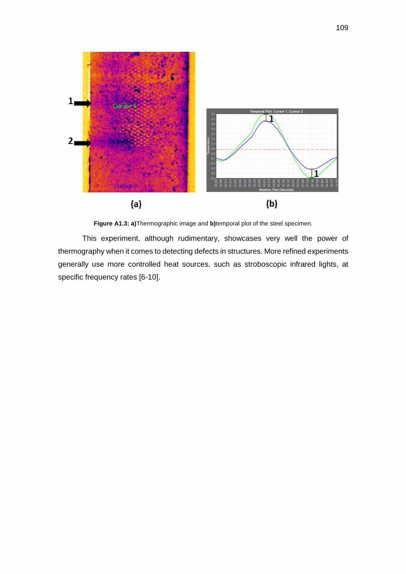
109
Figure A1.3: a)Thermographic image and b)temporal plot of the steel specimen.
This experiment, although rudimentary, showcases very well the power of
thermography when it comes to detecting defects in structures. More refined experiments
generally use more controlled heat sources, such as stroboscopic infrared lights, at
specific frequency rates [6-10].
DBD
PUC-Rio - Certificação Digital Nº 1412756/CA
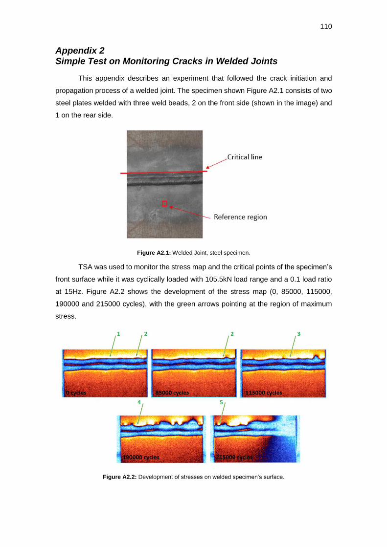
110
Appendix 2 Simple Test on Monitoring Cracks in Welded Joints
This appendix describes an experiment that followed the crack initiation and
propagation process of a welded joint. The specimen shown Figure A2.1 consists of two
steel plates welded with three weld beads, 2 on the front side (shown in the image) and
1 on the rear side.
Figure A2.1: Welded Joint, steel specimen.
TSA was used to monitor the stress map and the critical points of the specimen’s
front surface while it was cyclically loaded with 105.5kN load range and a 0.1 load ratio
at 15Hz. Figure A2.2 shows the development of the stress map (0, 85000, 115000,
190000 and 215000 cycles), with the green arrows pointing at the region of maximum
stress.
Figure A2.2: Development of stresses on welded specimen’s surface.
DBD
PUC-Rio - Certificação Digital Nº 1412756/CA
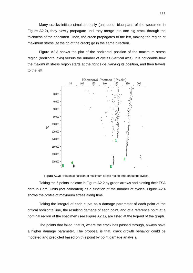
111
Many cracks initiate simultaneously (unloaded, blue parts of the specimen in
Figure A2.2), they slowly propagate until they merge into one big crack through the
thickness of the specimen. Then, the crack propagates to the left, making the region of
maximum stress (at the tip of the crack) go in the same direction.
Figure A2.3 shows the plot of the horizontal position of the maximum stress
region (horizontal axis) versus the number of cycles (vertical axis). It is noticeable how
the maximum stress region starts at the right side, varying its position, and then travels
to the left
Figure A2.3: Horizontal position of maximum stress region throughout the cycles.
Taking the 5 points indicate in Figure A2.2 by green arrows and plotting their TSA
data in Cam. Units (not calibrated) as a function of the number of cycles, Figure A2.4
shows the profile of maximum stress along time.
Taking the integral of each curve as a damage parameter of each point of the
critical horizontal line, the resulting damage of each point, and of a reference point at a
nominal region of the specimen (see Figure A2.1), are listed at the legend of the graph.
The points that failed, that is, where the crack has passed through, always have
a higher damage parameter. The proposal is that, crack growth behavior could be
modeled and predicted based on this point by point damage analysis.
DBD
PUC-Rio - Certificação Digital Nº 1412756/CA

112
Figure A2.4: TSA vs cycles curves for the maximum stress points.
Repeating the integration process, for all points along the critical horizontal line,
Figure A2.5 shows the plot of the damage parameter vs the horizontal position. It is
possible to see a trend where the cracked points show a higher damage result. More
tests are definitely required before any more speculation about the utility of this
parameter.
Figure A2.5: Damage for all points along the horizontal critical line.
DBD
PUC-Rio - Certificação Digital Nº 1412756/CA
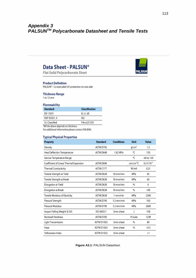
113
Appendix 3 PALSUNTM Polycarbonate Datasheet and Tensile Tests
Figure A3.1: PALSUN Datasheet.
DBD
PUC-Rio - Certificação Digital Nº 1412756/CA
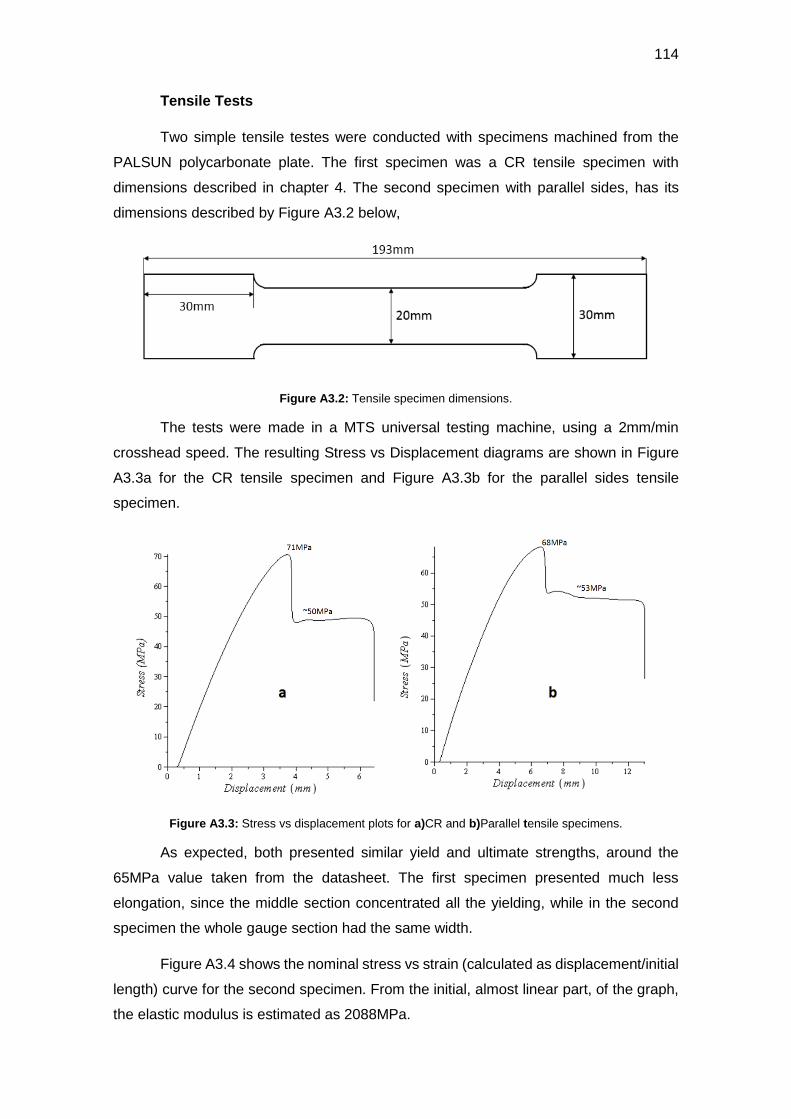
114
Tensile Tests
Two simple tensile testes were conducted with specimens machined from the
PALSUN polycarbonate plate. The first specimen was a CR tensile specimen with
dimensions described in chapter 4. The second specimen with parallel sides, has its
dimensions described by Figure A3.2 below,
Figure A3.2: Tensile specimen dimensions.
The tests were made in a MTS universal testing machine, using a 2mm/min
crosshead speed. The resulting Stress vs Displacement diagrams are shown in Figure
A3.3a for the CR tensile specimen and Figure A3.3b for the parallel sides tensile
specimen.
Figure A3.3: Stress vs displacement plots for a)CR and b)Parallel tensile specimens.
As expected, both presented similar yield and ultimate strengths, around the
65MPa value taken from the datasheet. The first specimen presented much less
elongation, since the middle section concentrated all the yielding, while in the second
specimen the whole gauge section had the same width.
Figure A3.4 shows the nominal stress vs strain (calculated as displacement/initial
length) curve for the second specimen. From the initial, almost linear part, of the graph,
the elastic modulus is estimated as 2088MPa.
DBD
PUC-Rio - Certificação Digital Nº 1412756/CA
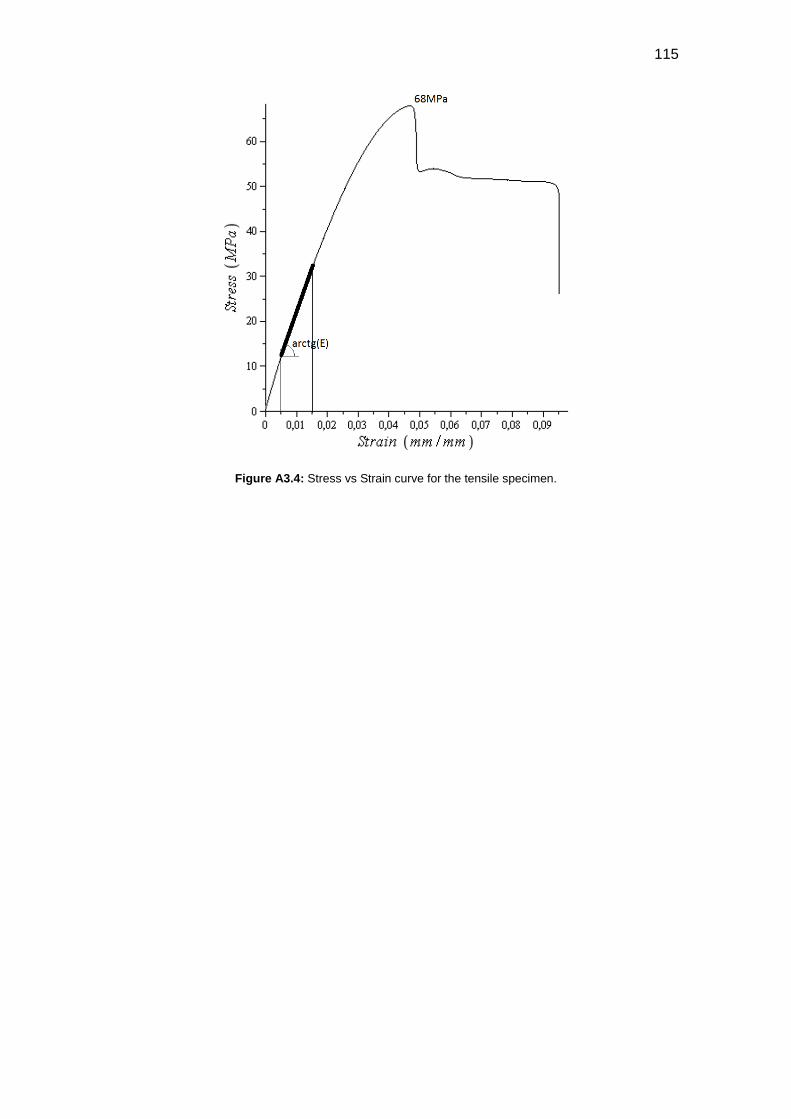
115
Figure A3.4: Stress vs Strain curve for the tensile specimen.
DBD
PUC-Rio - Certificação Digital Nº 1412756/CA

116
Appendix 4 Measuring the Keyhole Kt with DIC and Photoelasticity
In chapter 5, the stress concentration factor of the keyhole specimen was
measured using TSA. For verification purposes, it has also been measured via DIC and
Photoelasticity.
Photoelasticity
It is easy to use photoelasticity to analyze the stresses in a polycarbonate
specimen, since it is birefringent and it shows the isochromatic fringes seen through a
polariscope, that are the geometrical places of the points of constant σ1-σ2 value.
Measuring the Kt is once again facilitated because of the free surfaces boundary
condition that σ2=0. Figure A4.1 shows a series of photos taken of a statically loaded
polycarbonate keyhole specimen in a transmission polariscope and through a
monochromatic yellow filter. Table A4.1 shows the value of the load in each photo and
the distance each fringe is from the notch root, measured in pixels.
Figure A4.1: Series of Photoelastic photos.
Photo Load (N) Fr0 Fr1 Fr2 Fr3 Fr4 Fr5 Fr6 Fr7
1 20 260 - - - - - - -
2 40 275 36 - - - - - -
3 60 250 64 16 - - - - -
4 80 277 77 31 12 - - - -
5 100 270 85 42 22 8 - - -
6 120 281 101 54 31 17 8 - -
7 140 281 109 65 40 25 15 7 -
8 160 279 120 71 46 30 20 12 6
Table A4.1: Fringe distance from notch tip.
DBD
PUC-Rio - Certificação Digital Nº 1412756/CA
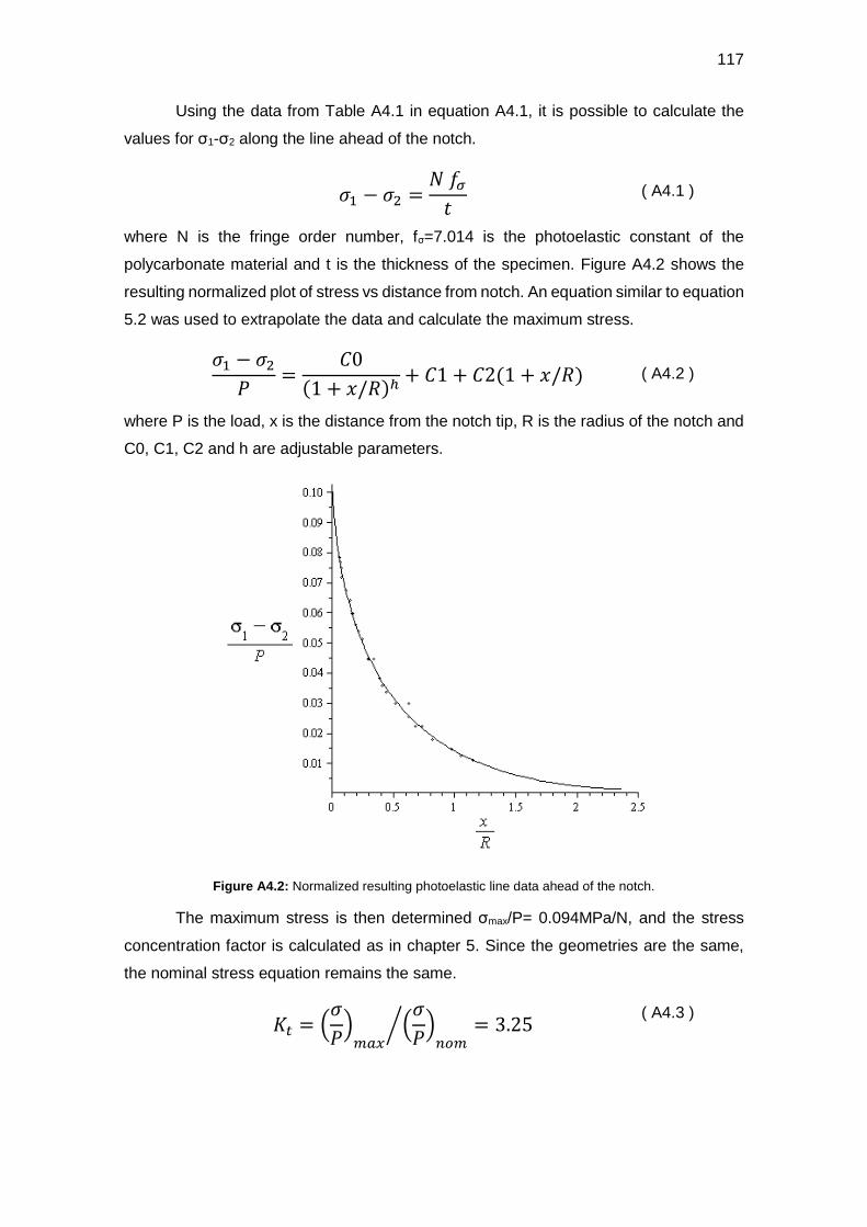
117
Using the data from Table A4.1 in equation A4.1, it is possible to calculate the
values for σ1-σ2 along the line ahead of the notch.
𝜎1 − 𝜎2 =𝑁𝑓𝜎𝑡
( A4.1 )
where N is the fringe order number, fσ=7.014 is the photoelastic constant of the
polycarbonate material and t is the thickness of the specimen. Figure A4.2 shows the
resulting normalized plot of stress vs distance from notch. An equation similar to equation
5.2 was used to extrapolate the data and calculate the maximum stress.
𝜎1 − 𝜎2𝑃
=𝐶0
(1 + 𝑥/𝑅)ℎ+ 𝐶1 + 𝐶2(1 + 𝑥/𝑅) ( A4.2 )
where P is the load, x is the distance from the notch tip, R is the radius of the notch and
C0, C1, C2 and h are adjustable parameters.
Figure A4.2: Normalized resulting photoelastic line data ahead of the notch.
The maximum stress is then determined σmax/P= 0.094MPa/N, and the stress
concentration factor is calculated as in chapter 5. Since the geometries are the same,
the nominal stress equation remains the same.
𝐾𝑡 = (𝜎
𝑃)𝑚𝑎𝑥
(𝜎
𝑃)𝑛𝑜𝑚
⁄ = 3.25 ( A4.3 )
DBD
PUC-Rio - Certificação Digital Nº 1412756/CA

118
Digital Image Correlation
DIC is another optical experimental stress analysis technique, which has been
one of the main research topics in recent days` experimental mechanics. It consists in
an algorithm capable of identifying surfaces features before and after a load is applied
to a specimen, and then, by correlating the positions of such features, the full field of
displacements is determined. The displacements field can be differentiated to obtain the
strains field. With the strain field in hands, using a stress-strain relationship (such as
Hooke`s law for elastic regime) will yield the stress field acting on the surface.
The first step when using DIC is to paint the target surface with a specific pattern
with many features that the software can recognize. Figure A4.3 shows the surface of
the keyhole specimen painted with the pattern.
Figure A4.3: DIC pattern.
Then, by taking a photo of the unloaded specimen and another with the specimen
loaded at P= 255N, and running the ViC3DTM software from Correlated Solutions Inc.,
the strain fields are calculated. Figure A4.4 shows the principal strain field (ε1), and
Figure A4.5 shows the normalized plot of stresses vs distance from notch, the stress-
strain relationship used was the plane stress Hooke`s law described by equation A4.4.
[
𝜎1𝜎2𝜎12
] =𝐸
1 − 𝜈2[
1 𝜈 0𝜈 1 0
0 01 − 𝜈
2
] [
휀1휀22휀12
]
( A4.4 )
where σ`s are the stress components, ε`s are the strain components, E is the material
Young`s modulus (E= 2300MPa for polycarbonate) and ν is the Poisson`s coefficient (ν=
0.39 for polycarbonate).
DBD
PUC-Rio - Certificação Digital Nº 1412756/CA

119
Figure A4.4: DIC principal strain field result.
Figure A4.5: DIC stress results ahead of the notch.
Following the same procedure as before, equation A4.5 is used to fit the σ1 data
and to extrapolate the value of the maximum principal stress.
𝜎1𝑃=
𝐶0
(1 + 𝑥/𝑅)ℎ+ 𝐶1 + 𝐶2(1 + 𝑥/𝑅)
( A4.5 )
The resulting graph is shown in Figure A4.6.
DBD
PUC-Rio - Certificação Digital Nº 1412756/CA

120
Figure A4.6: DIC fitted principal stress ahead of the notch.
The resulting maximum stress obtained was σmax/P= 0.095MPa/N, and the stress
concentration factor is calculated as in chapter 5, since the geometries are the same,
the nominal stress remains the same.
𝐾𝑡 = (𝜎
𝑃)𝑚𝑎𝑥
(𝜎
𝑃)𝑛𝑜𝑚
⁄ = 3.27 ( A4.6 )
DBD
PUC-Rio - Certificação Digital Nº 1412756/CA

121
Appendix 5 Finite Elements Analysis of the Keyhole Specimen
A Finite Elements Analysis (FEA) was made on the keyhole specimen, in order
to evaluate the stress concentration factor and the stress intensity factors. This appendix
describes these analyses made using ANSYS Workbench 15.0.
Stress Concentration Factor
In order to evaluate the Kt of the keyhole, a symmetric finite elements model was
made, with the dimensions show in chapter 4. The meshed model is shown in Figure
A5.1
Figure A5.1: Meshed symmetric model for FEA of the keyhole specimen.
The load (100N) was applied as a bearing load at the pin-hole and the constraint
was of no vertical displacement at the symmetry plane. The resulting σy map is shown
by Figure A5.2.
Figure A5.2: FEA resulting σy map for the keyhole specimen.
DBD
PUC-Rio - Certificação Digital Nº 1412756/CA

122
As expected, the stress varies along the thickness at the notch tip, Figure A5.3
shows the plot of stress concentration factor vs thickness, being the maximum value, at
the middle point, Kt max=3.17 and the minimum value, at the borders, Kt min=3.02.
Figure A5.3: Kt vs thickness plot for the keyhole specimen.
Stress Intensity Factors
The evaluation of the SIF was done through the fracture tool of ANSYS
Workbench. Using the pre-meshed crack option to model the crack, and refining the
mesh around its tip, Figure A5.4 shows the resulting meshed model (a=10mm) and the
refined region, symmetry was not used because the pre-meshed crack do not allow it.
Figure A5.4: Meshed model for SIF evaluation of the keyhole specimen.
DBD
PUC-Rio - Certificação Digital Nº 1412756/CA

123
Again, the load (100N) was applied as a bearing load at the top pin-hole. The
constraint, on the other hand, was added as a bearing support at the bottom pin-hole.
The resulting σy map is shown in Figure A5.5.
Figure A5.5: FEA resulting σy map for cracked (a=10mm) keyhole specimen.
The thickness effect makes the SIF vary along the thickness just as the Kt did.
Figure A5.6 shows the plot of K1/P vs thickness, as determined by the 6th contour in the
fracture tool. The maximum and minimum values are 0.00705 and 0.00589 respectively.
Figure A5.6: KI/P vs thickness plot for the cracked a=10mm) keyhole specimen.
DBD
PUC-Rio - Certificação Digital Nº 1412756/CA

124
The analysis was repeated for several crack sizes varying from 0.1mm to 30mm,
Figure A5.7 shows the plot of KI/P vs a for the middle point and for the border of the
cracked keyhole specimen.
Figure A5.7: KI/P vs a plot for the keyhole specimen.
Polynomials were used to fit the data resulting in two equations with correlation
R2 also shown in Figure A5.7.
DBD
PUC-Rio - Certificação Digital Nº 1412756/CA

125
Appendix 6 Photos of the Specimens
This appendix shows a series of photos taken from the fracture surfaces, fatigue
cracks and fretting cracks of all specimens used throughout the entire study.
Each image has text boxes explaining key features, and are listed below in three
categories:
DBD
PUC-Rio - Certificação Digital Nº 1412756/CA

126
Fracture surfaces
Figure A6.1: Fracture surface of CR tensile specimen after tensile test.
Figure A6.2: Fracture surface of tensile specimen after tensile test.
DBD
PUC-Rio - Certificação Digital Nº 1412756/CA
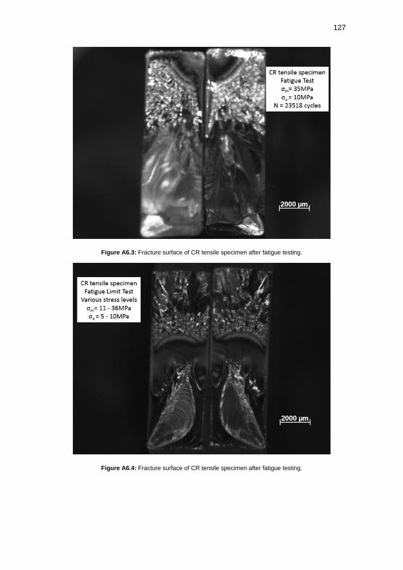
127
Figure A6.3: Fracture surface of CR tensile specimen after fatigue testing.
Figure A6.4: Fracture surface of CR tensile specimen after fatigue testing.
DBD
PUC-Rio - Certificação Digital Nº 1412756/CA

128
Figure A6.5: Fracture surface of CR tensile specimen after fatigue bending testing.
Figure A6.6: Fracture surface of CR tensile specimen after fatigue testing.
DBD
PUC-Rio - Certificação Digital Nº 1412756/CA
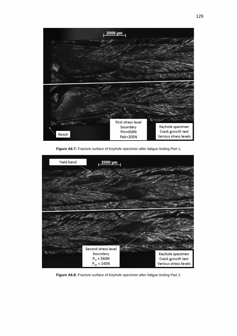
129
Figure A6.7: Fracture surface of Keyhole specimen after fatigue testing Part 1.
.
Figure A6.8: Fracture surface of Keyhole specimen after fatigue testing Part 2.
DBD
PUC-Rio - Certificação Digital Nº 1412756/CA
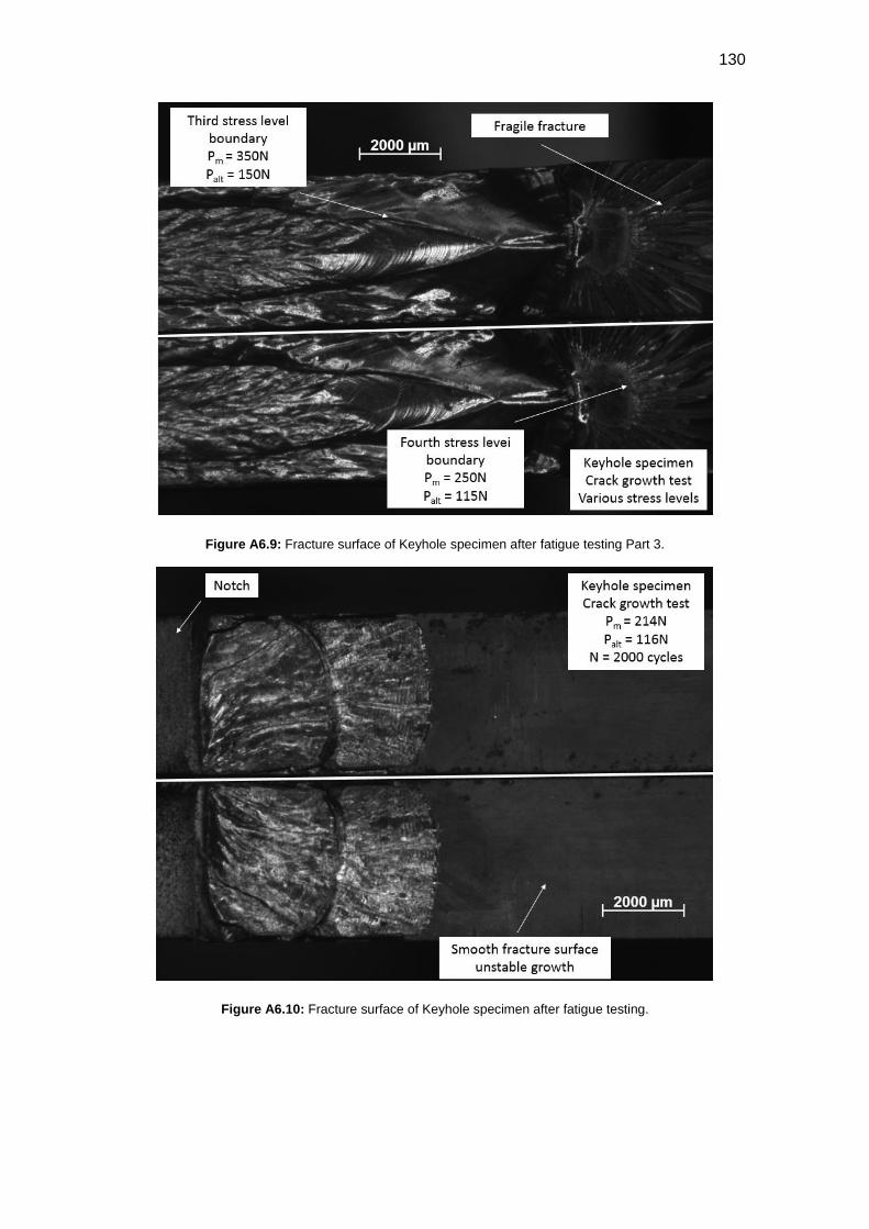
130
Figure A6.9: Fracture surface of Keyhole specimen after fatigue testing Part 3.
Figure A6.10: Fracture surface of Keyhole specimen after fatigue testing.
DBD
PUC-Rio - Certificação Digital Nº 1412756/CA
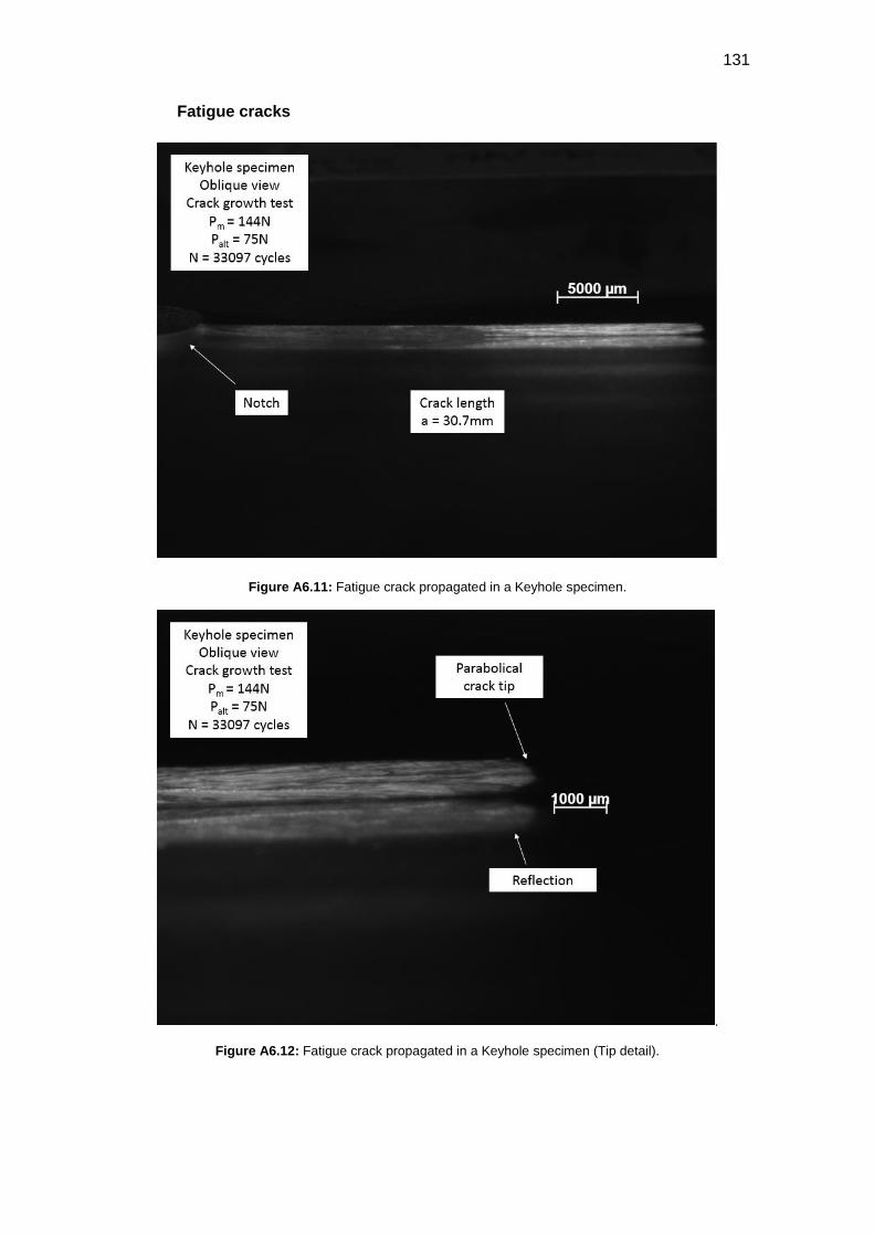
131
Fatigue cracks
Figure A6.11: Fatigue crack propagated in a Keyhole specimen.
.
Figure A6.12: Fatigue crack propagated in a Keyhole specimen (Tip detail).
DBD
PUC-Rio - Certificação Digital Nº 1412756/CA

132
Figure A6.13: Fatigue crack propagated in a Keyhole specimen.
Figure A6.14: Fatigue crack propagated in a Keyhole specimen (Tip detail).
DBD
PUC-Rio - Certificação Digital Nº 1412756/CA
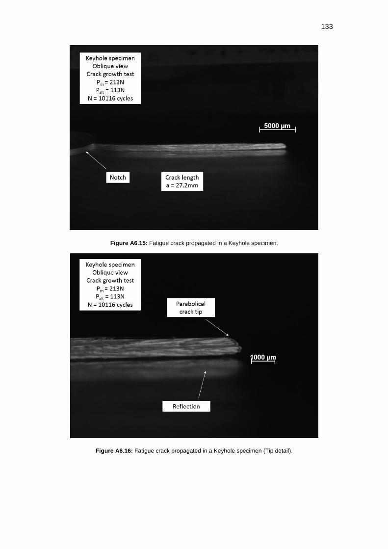
133
Figure A6.15: Fatigue crack propagated in a Keyhole specimen.
Figure A6.16: Fatigue crack propagated in a Keyhole specimen (Tip detail).
DBD
PUC-Rio - Certificação Digital Nº 1412756/CA

134
Figure A6.17: Fatigue crack propagated in a Keyhole specimen.
Figure A6.18: Fatigue crack propagated in a Keyhole specimen (Tip detail).
DBD
PUC-Rio - Certificação Digital Nº 1412756/CA

135
Figure A6.19: Fatigue crack propagated in a Keyhole specimen.
Figure A6.20: Fatigue crack propagated in a Keyhole specimen (Tip detail).
DBD
PUC-Rio - Certificação Digital Nº 1412756/CA

136
Fretting cracks
Figure A6.21: Fretting damage and crack initiation in a CR tensile specimen.
Figure A6.22: Fretting damage and crack initiation in a CR tensile specimen.
DBD
PUC-Rio - Certificação Digital Nº 1412756/CA

137
Figure A6.23: Fretting crack in a CR tensile specimen (front view).
Figure A6.24: Fretting crack in a CR tensile specimen (oblique view).
DBD
PUC-Rio - Certificação Digital Nº 1412756/CA

138
Figure A6.25: Fretting fracture surface.
Figure A6.26: Fretting fracture surface (zoom).
DBD
PUC-Rio - Certificação Digital Nº 1412756/CA

139
Figure A6.27: Fretting fracture surface (initiation detail).
DBD
PUC-Rio - Certificação Digital Nº 1412756/CA