Removing the Stiffness of Elastic Force from the Immersed

Boundary Method for the 2D Stokes Equations

Thomas Y. Hou∗ Zuoqiang Shi †

June 16, 2007

Abstract

The Immersed Boundary method has evolved into one of the most useful computa-tional methods in studying fluid structure interaction. On the other hand, the ImmersedBoundary method is also known to suffer from a severe timestep stability restriction whenusing an explicit time discretization. In this paper, we propose several efficient semi-implicit schemes to remove this stiffness from the Immersed Boundary method for thetwo-dimensional Stokes flow. First, we obtain a novel unconditionally stable semi-implicitdiscretization for the immersed boundary problem. Using this unconditionally stable dis-cretization as a building block, we derive several efficient semi-implicit schemes for theimmersed boundary problem by applying the Small Scale Decomposition to this uncondi-tionally stable discretization. Our stability analysis and extensive numerical experimentsshow that our semi-implicit schemes offer much better stability property than the explicitscheme. Unlike other implicit or semi-implicit schemes proposed in the literature, our semi-implicit schemes can be solved explicitly in the spectral space. Thus the computationalcost of our semi-implicit schemes is comparable to that of an explicit scheme, but with amuch better stability property.

1 Introduction

The Immersed Boundary method was originally introduced by Peskin in the 1970’s to modelthe flow around heart valves. Now it has evolved into a general useful method in studying themotion of one or more massless, elastic surface immersed in an incompressible, viscous fluid,particularly in biofluid dynamics problems where complex geometries and immersed elasticmembranes are present. The method has been successfully applied to a variety of problemsincluding blood flow in the heart [25, 16, 17, 18, 26, 19, 20], vibrations of the cochlear basilarmembrane [2, 8], platelet aggregation during clotting [7, 34], aquatic locomotion [5, 6, 11, 35, 3],flow with suspended particles [5, 31], and inset flight [21, 22], We refer to [27] for an extensivelist of applications.

The Immersed Boundary method employs a uniform Eulerian grid over the entire domainto describe the velocity field of the fluid and a Lagrangian description for the immersed elastic

∗Applied and Comput. Math, Caltech, Pasadena, CA 91125. Email: hou@acm.caltech.edu.†Applied and Comput. Math, Caltech, Pasadena, CA 91125 and Zhou Pei-Yuan Center for Applied Mathe-

matics, Tsinghua University, Beijing 100084, China. Email: shi@acm.caltech.edu.

1

structure. The force generated by the elastic structure drives the fluid and the fluid movesthe elastic structure. This interaction is expressed in terms of the spreading and interpolationoperations by use of smoothed Delta functions.

One of the main difficulties that the Immersed Boundary method encounters is that itsuffers from a severe timestep restriction in order to keep the stability [27, 32, 30]. This hasbeen the major limitation of the Immersed Boundary method. This restriction is typicallymuch more severe than the one that would be imposed from using an explicit discretization forthe convection term in the Navier-Stokes equation. The instability is known to arise from largeboundary force and small viscosity [32]. Much effort has been made to remove this restriction.Some implicit and semi-implicit methods have been proposed in the literature [33, 23, 15].Despite of these efforts, the timestep restriction has not been resolved satisfactorily. Thecomputational cost of using an implicit or semi-implicit scheme is still too high to be effectivein a practical computation. To date, almost all practical computations using the immersedboundary method have been performed using an explicit discretization.

In this paper, we develop several efficient semi-implicit schemes to compute the motionof an elastic interface immersed in a two-dimensional, incompressible Stokes flow. There areseveral important ingredients in deriving our semi-implicit schemes. The first one is to use thearclength and tangent angle formulation to describe the dynamics of the immersed interface[9]. We remark that Ceniceros and Roma have also used the arclength and tangent angleformulation to alleviate the stiffness of the viscous vortex sheet with surface tension in [4]. Thesecond one is to obtain an unconditionally stable semi-implicit discretization of the immersedboundary problem. Throughout this paper, we use the term “stability” to mean that the energynorm of the solution can be bounded in terms of the energy norm of the initial data, which isa weaker result than proving that the difference between two solutions in the energy norm canbe bounded in terms of the energy norm of their difference at time zero. The third ingredientis to perform Small Scale Decomposition to the unconditionally stable discretization to obtainour efficient semi-implicit schemes. An important feature of our small scale decompositionis that the leading order term, which is to be discretized implicitly, can be expressed as aconvolution operator. This property enables us to solve for the implicit solution explicitlyusing the Fourier transformation. Thus, the computational cost of our semi-implicit schemesis comparable to that of an explicit method. This offers a significant computational saving inusing the Immersed Boundary method.

The Small Scale Decomposition was first developed by Hou, Lowengrub and Shelley [9, 10].They applied this method to remove the stiffness from interfacial flow with surface tension,which has proved to be very successful. Due to the coupling between the elastic boundarywith the fluid, it is more difficult to remove the stiffness induced by the elastic force in theImmersed Boundary method. To remove the stiffness in the Immersed Boundary method,we need to decouple the stiffness induced by the elastic force from the fluid flow in such away that the resulting semi-implicit discretization is still unconditionally stable. This is ac-complished by using a semi-implicit discretization which preserves certain important solutionstructures which exist at the continuous level. Without obtaining this unconditionally stablesemi-implicit discretization, a straightforward application of the Small Scale Decompositionto the Immersed Boundary method would not provide an efficient semi-implicit scheme withthe desirable stability property. Very recently, Newren et al. have obtained an uncondition-ally stable discretization for linear force in [24]. However, they did not perform Small Scale

2

Decomposition to their unconditionally stable discretization. As we will demonstrate in thispaper, the unconditionally stable semi-implicit discretization without using the Small ScaleDecomposition is still very expensive and the gain over the explicit discretization is quitelimited.

We develop several efficient semi-implicit schemes for both the steady Stokes flow and theunsteady Stokes flow respectively. In both cases, our semi-implicit schemes work very well.In the steady Stokes flow, we also develop a fourth order semi-implicit scheme by using theintegral factor method. For the unsteady Stokes flow, we develop a second order semi-implicitmethod by combining our Small Scale Decomposition with a well known second order temporaldiscretization [13, 27]. To illustrate the stability properties of our semi-implicit schemes, weapply our methods to several prototype problems and test our schemes for a range of elasticcoefficients and viscosity coefficients. Our numerical results confirm that the semi-implicitschemes remove the high order stability constraint induced by the elastic force. In the caseof unsteady Stokes equation, we also confirm the second order accuracy of our semi-implicitscheme.

This paper is organized as follows. First, we review the classical formulation of the Im-mersed Boundary method in Section 2. Then, we introduce the arclength and tangent angleformulation in Section 3. In Section 4, we describe the spatial discretization of the ImmersedBoundary method. In Section 5-6, we develop the numerical schemes for steady Stokes flowand unsteady Stokes flow respectively. The numerical results are presented in Section 7. Ournumerical studies will focus on the stability restriction and computational cost of our methods.Some concluding remarks are given in Section 8.

2 Review of the Immersed Boundary method

For simplicity, we just consider a viscous incompressible fluid in a two dimensional domainΩ, containing an immersed massless elastic boundary in the form of a closed simple curveΓ. The configuration of the boundary is given in a parametric form: X(α, t), 0 ≤ α ≤ Lb,X(0, t) = X(Lb, t), α tracks a material point of the boundary. We consider only the Stokesequations in this paper and would neglect the convection term. Then the governing equationsare given as follows:

ρ∂u

∂t= −∇p+ µ4u + f(x, t) , (1)

∇ · u = 0 , (2)

∂X

∂t(α, t) = u(X(α, t), t) , (3)

where u is the fluid velocity, p is the pressure, ρ and µ are constant fluid density and viscosity,f(x, t) is the force density, which is not zero only on the boundary and which is infinite there.The force density can be expressed as below

f(x, t) =

∫ Lb

0F(α, t)δ(x −X(α, t))dα, (4)

δ denotes the two-dimensional Dirac delta function and

F(α, t) =∂

∂α(Tτ ), (5)

3

T = T

(∣∣∣∣∂X

∂α

∣∣∣∣). (6)

The choice of function T in this paper is computed by Hook’s law

T = Sb

(∣∣∣∣∂X

∂α

∣∣∣∣− 1

), (7)

where Sb is the elastic coefficient of the boundary, and τ is the unit tangent vector along theboundary, which is defined as

τ =∂X

∂s

/∣∣∣∣∂X

∂s

∣∣∣∣ . (8)

This choice of force density has been used widely in the literature in both computational andtheoretical studies [12],[29],[33].

We can rewrite (3) in the following way:

∂X

∂t(α, t) =

∫

Ωu(x, t)δ(x −X(α, t))dx. (9)

Next, we introduce the spreading and interpolation operations. The spreading and interpola-tion operators are defined as follows:

L(X)(g(α))(x) =

∫

Γg(α)δ(x −X(α, t))dα, (10)

L∗(X)(u(x))(α) =

∫

Ωu(x)δ(x −X(α, t))dx . (11)

It is easy to show that L and L∗ are adjoint operators:

< u(x), L(X)(g(α)) >Ω

=

∫

Ωu(x)

(∫

Γg(α)δ(x −X(α, t))dα

)dx

=

∫

Ω

∫

Γu(x)g(α)δ(x −X(α, t))dαdx

=

∫

Γ

∫

Ωu(x)g(α)δ(x −X(α, t))dxdα

=

∫

Γg(α)

(∫

Ωu(x)δ(x −X(α, t))dx

)dα

= < L∗(X)(u(x)), g(α) >Γ , (12)

where the inner product are defined as follows:

< u, v >Ω =

∫

Ωu(x)v(x)dx, (13)

< f, g >Γ =

∫

Γf(α)g(α)dα. (14)

Equations (1),(2) are the familiar Stokes equations of viscous incompressible fluid. Equa-tions (3),(4) represent the interaction of the fluid and the elastic boundary. The elastic bound-ary applies the force to the fluid, the fluid carries the immersed boundary, and the force densityis determined by the configuration of the boundary.

4

3 The arclength-tangent angle formulation

In studying the evolution of a curve, it is useful to represent the curve by its tangent angle θand local arclength derivative sα. Previously, Hou, Lowengrub and Shelley [9] exploited thisformulation and combined it with a so-called ”Small Scale Decomposition” reformulation toremove the stiffness induced by surface tension.

Consider the evolution of a simply closed curve Γ with known normal and tangent velocityfields, U, V . Assume the curve is represented by X(α, t), α ∈ [0, Lb]. We define the arclengthderivative, sα, and the tangent vector, θ, as follows

sα(α, t) = |Xα(α, t)|, (15)

(xα(α, t), yα(α, t)) = sα(α, t)(cos θ(α, t), sin θ(α, t)). (16)

The closed curve Γ evolves according to

∂X

∂t= u(X, t) = Un + V τ , (17)

where τ and n are the unit tangent and normal vectors of the curve respectively. Accordingto the Frenet formula, we have ∂τ

∂s = kn, ∂n

∂s = −kτ , here s is the arclength variable. It is easyto see that sα and θ satisfy the following evolution equations [9]:

(sα)t = Vα − θαU, (18)

θt =Uα

sα+V θα

sα. (19)

Given sα and θ, the curve Γ can be reconstructed up to a translation by integrating (16).However, we also need a point on the boundary to provide the constant of integration.

Using the sα − θ formulation, we can reformulate the immersed boundary problem asfollows:

ρ∂u

∂t= −∇p+ µ4u + L(X) (F(sα, θ)) , (20)

∇ · u = 0 (21)

U = L∗(X)(u(x)) · n, (22)

V = L∗(X)(u(x)) · τ , (23)

(sα)t = Vα − θαU, (24)

θt =Uα

sα+V θα

sα, (25)

where

F(sα, θ) =∂

∂α(Tτ ) = Sb (sα,ατ + (sα − 1)θαn) . (26)

4 Spatial Discretization

We use the spectral method to discretize both the Stokes equations and the immersed boundaryequations in space since we work on periodic domains. We first discuss the discretization of the

5

Stokes equations in a regular N ×N Cartesian grid with a uniform meshsize h. Let xj = jhand yj = jh. The discrete Fourier transform and inverse Fourier transform are defined asfollows:

Fh,x(φ)(k, y) =1

N

N−1∑

j=0

φ(xj , y)e−ikxj = φ(k, y), −N/2 + 1 ≤ k ≤ N/2, (27)

Fh,y(φ)(x, k) =1

N

N−1∑

j=0

φ(x, yj)e−ikyj = φ(x, k), −N/2 + 1 ≤ k ≤ N/2, (28)

F−1h,x(φ)(xj , y) =

N/2∑

k=−N/2+1

φ(k, y)eikxj = φ(xj , y), 0 ≤ j ≤ N − 1, (29)

F−1h,y(φ)(x, yj) =

N/2∑

k=−N/2+1

φ(x, k)eikyj = φ(x, yj), 0 ≤ j ≤ N − 1. (30)

Now we introduce the discrete differential operator using the discrete Fourier transform de-fined above. For a function φ(x, y) defined in the fluid domain Ω, we approximate its spatialderivatives as follows:

(Dh,xφ) (x, y) = F−1h,x (ik (Fh,xφ) (k, y)) , (31)

(Dh,yφ) (x, y) = F−1h,y (ik (Fh,yφ) (x, k)) . (32)

Denote ∇h = (Dh,x, Dh,y). The differential operators are discretized in terms of Dh:

∇p → ∇hp, (33)

∇ · u → ∇h · u, (34)

∇2u → ∇h · ∇h u ≡ ∇2hu. (35)

Next, we describe the discretization of the immersed boundary. We employ a Lagrangiangrid with grid space ∆α. The number of grid points along the boundary is Nb. For a functionψ(α) defined on the interface Γ, we define the discrete Fourier transform and its inverse asfollows:

F∆α(ψ)(k) =1

Nb

Nb−1∑

j=0

φ(αj)e−ikαj = ψ(k), αj = j∆α, (36)

F−1∆α(ψ)(αj) =

Nb2∑

k=−Nb2

+1

ψ(k)eikαj = ψ(αj). (37)

When the interface is a closed curve, we can approximate the derivative operator along theinterface by the spectral derivative:

(D∆αψ) (α) = F−1∆α (ik (F∆αφ) (k)) . (38)

When the solution is not periodic, we can also use a finite difference method to discretize thederivative, we refer to [27] for more details.

6

Now we discuss the discretization of the spreading and interpolation operators. These twooperators both involve the use of a discrete delta function. The discrete delta function we useis introduced by Peskin in [27]:

δh(x, y) =1

h2φ

(x

h

)φ

(y

h

), (39)

and

φ(r) =

18

(3 − 2|r| +

√1 + 4|r| − 4r2

), |r| ≤ 1,

18

(5 − 2|r| −

√−7 + 12|r| − 4r2

), 1 ≤ |r| ≤ 2,

0, |r| > 2.

(40)

Using the above discrete delta function, we can discretize the spreading and interpolationoperator as follows

Lh(X)(g(α))(x) =∑

α∈GΓ

g(α)δh(x −X(α, t))∆α, (41)

L∗h(X)(u(x))(α) =

∑

x∈GΩ

u(x)δh(x−X(α, t))h2. (42)

The summation above is over grid points in Γ in (41) and over grid points in Ω in (42). OperatorLh and L∗

h are still adjoint using the following discrete inner product:

< f, g >Γh=∑

α∈GΓ

f(α)g(α)∆α, (43)

< u, v >Ωh=∑

x∈GΩ

u(x)v(x)h2. (44)

Using the inner product defined above, we have:

< u(x), L(X)(g(α)) >Ωh

=∑

x∈GΩ

u(x)L(X)(g(α))h2

=∑

x∈GΩ

u(x)h2∑

α∈GΓ

g(α)δh(x −X(α, t))∆α

=∑

x∈GΓ

g(α)∆α∑

α∈GΩ

u(x)δh(x −X(α, t))h2

= < L∗h(X)(u(x)), g(α) >Γh

. (45)

As we will see later, this discrete self-adjoint property is crucial in obtaining our unconditionalstable semi-discrete scheme for the immersed boundary problem.

5 Steady Stokes flow

5.1 Formulation

For simplicity, we study the steady Stokes flow first. The governing equations for the steadyStokes flow are given as follows:

0 = −∇p+ µ4u + L(X) (F(sα, θ)) , (46)

7

∇ · u = 0, (47)

U = u(X(α, t), t) · n, (48)

V = u(X(α, t), t) · τ , (49)

(sα)t = Vα − θαU, (50)

θt =Uα

sα+V θα

sα. (51)

In this simple case, we can use a boundary integral method for the two dimension Stokesflow (page 60 of [28]) to solve equations (46)-(47) to get the velocity on the boundary:

u(X(α, t)) =1

4πµ

∫

Γ

(−(ln r)F1(α

′, t) +r21r2F1(α

′, t) +r1r2r2

F2(α′, t)

)dα′, (52)

v(X(α, t)) =1

4πµ

∫

Γ

(−(ln r)F2(α

′, t) +r22r2F2(α

′, t) +r1r2r2

F1(α′, t)

)dα′, (53)

where r = |r| and

r = (r1, r2) = X(α, t) −X(α′, t), F = (F1, F2), u = (u, v). (54)

5.2 Small Scale Decomposition

As we can see from (52)-(53), the velocity field can be expressed as a singular integral with akernel ln(r). However, the singular velocity integral is nonlinear and nonlocal. It is difficultto solve for the implicit solution if we treat the velocity integral fully implicitly. The mainidea of the Small Scale Decomposition technique introduced in [9] is to decompose the singularvelocity integral into the sum of a linear singular operator which is a convolution operatorindependent of time t and the configuration of the curve, and a remainder operator which isregular. Since the remaining operator, which is nonlinear and nonlocal, is regular, the sim-plified convolution integral operator captures accurately the high frequency spectral propertyof the original velocity integral. Thus, if we treat only the leading order convolution operatorimplicitly, but keep the regular remainder operator explicitly, we can effectively remove thestiffness of the original velocity field which comes mainly from the high frequency modes ofthe solution. In this subsection, we will show how to perform such Small Scale Decompositionfor the Immersed Boundary method applied to the Stokes flow.

Observe that in the integral representation of the velocity field, (52)-(53), the only singularpart of the kernel is ln(r). The other part of the kernel is smooth. Thus to the leading ordercontribution of the velocity field can be expressed as follows:

u(X(α, t)) ∼ 1

4πµ

∫

Γ−(ln r)F(α′, t)dα′, (55)

V = u(X(α, t), t) · τ (α) (56)

∼ 1

4πµ

∫

Γ−(ln r)F(α′, t) · τ (α)dα′

=Sb

4πµ

∫

Γ−(ln r)

(sα,α′τ (α′) + (sα − 1)θα′n(α′)

)· τ (α)dα′. (57)

8

Next, we perform a Taylor expansion for r, τ (α′) · τ (α) and n(α′) · τ (α) as a function of α′

around α. By keeping only the leading order term, we have

r ∼ sα(α)|α − α′|, (58)

τ (α′) · τ (α) ∼ 1, (59)

n(α′) · τ (α) ∼ 0. (60)

Substituting the above Taylor expansions to (56), we get

V ∼ Sb

4πµ

∫ln(sα(α)|α − α′|

)sα,α′dα′. (61)

Integrating by part, we obtain

V ∼ Sb

4πµ

∫sα′

α′ − αdα′ = −Sb

4µH[sα], (62)

where H is the Hilbert transform

H[f ](α) =1

π

∫ +∞

−∞

f(α′)

α− α′dα′. (63)

Using the same method, we can get the leading order contributions of U and Uα as follows:

U ∼ Sb

4πµ

∫− ln |α− α′|(sα′ − 1)θα′dα′ (64)

Uα ∼ Sb

4πµ

∫(sα′ − 1)θα′

α′ − αdα′ = −Sb

4µH[(sα − 1)θα]. (65)

Note that if f is a smooth function, then the commutator [H, f ]u ≡ H(fu) − fH(u) is asmoothing operator for u. Thus we can factor a smooth function from the Hilbert transformwithout changing its leading order spectral property. Suppose that sα is smooth, then weobtain to the leading order that

Uα ∼ −Sb

4µ(sα − 1)H[θα]. (66)

Applying the same analysis to the Eqs (115)-(116) gives

(sα)t = −Sb

4µH[D∆αsα] +

(D∆αV −D∆αθU +

Sb

4µH[D∆αsα]

), (67)

θt = −Sb

4µ

(1 − 1

sα

)H[D∆αθ] +

(D∆αU

sα+V D∆αθ

sα+Sb

4µ

(1 − 1

sα

)H[D∆αθ]

). (68)

Note that the leading order operator is linear. This suggests a natural semi-implicit discretiza-tion of the immersed boundary problem.

Since we are dealing with a closed immersed boundary, it is natural to work in the Fourierspace. Furthermore, the Hilbert operator has a very simple kernel under the Fourier trans-formation. Notice that θ is not a periodic function of α. Its value increases 2π every time αincreases Lb. Nevertheless, if we let

θ(α, t) =2π

Lbα+ φ(α, t), α ∈ [0, Lb], (69)

9

then φ is periodic. It is more convenient to work with φ than θ. Substituting (69) into (68)and taking the Fourier transform on both sides of (67),(68), we obtain

sα,t = −Sb

4µ|k|sα +

[F (D∆αV −D∆αθU) +

Sb

4µ|k|sα

], (70)

φt = −Sb

4µγ|k|φ+

[F(D∆αU

sα+V D∆αθ

sα

)+Sb

4µγ|k|φ

], (71)

where γ = maxα

(1 − 1

sα

). We have also used the fact that Hk = −i sgn(k) with sgn(k) being

the signature function. The first term on the right hand side captures the leading order highfrequency contribution of the terms from the right hand side. An important property of thisleading order term is that it is linear in sα and θ and has constant coefficient in space. Thisprovides a straightforward application of the implicit time discretization.

Since our small scale decomposition is exact near the equilibrium, we can use this result toget the stability constraint of the explicit scheme by using a frozen coefficient analysis. Thestability constraint is given by

∆t < Cµ

Sb

h

γ. (72)

As we can see, the time step needs to be very small if Sb is large and µ is small. For example,if Sb = 100, and µ = 10−2, then the stability would require that ∆t ≤ C10−4h.

5.3 Semi-implicit schemes

Based on the small scale decomposition presented in the previous subsection, we propose twotypes of semi-implicit schemes in this section. The first implicit time discretization uses thebackward Euler method to discretize the leading order term while keeping the lower order termexplicit. This gives rise to the following semi-implicit scheme:

sn+1α − sn

α

∆t= −Sb

4µ|k|sn+1

α +

[F (D∆αV

n −D∆αθnUn) +

Sb

4µ|k|sn

α

], (73)

φn+1 − φn

∆t= −Sb

4µγ|k|φn+1 +

[F(D∆αU

n

sn+1α

+V nD∆αθ

n

sn+1α

)+Sb

4µγ|k|φn

]. (74)

We call the above discretization the semi-implicit method. Near equilibrium, the stabilityconstraint of this numerical method is ∆t < C(Sb, µ), independent of the meshsize h. Sincethe small scale decomposition only captures the leading order contribution from the highfrequency components, this method can not eliminate the effect of Sb and µ completely. Thecoefficients Sb and µ can still affect the time stability through the low frequency componentsof the solution, which comes from the second term of the right hand side. In order to obtain asemi-implicit discretization with better stability property, we can incorporate the low frequencycontribution from the second term in our implicit discretization. This scheme can be found inthe appendix A. We call it the semi-implicit scheme of second kind.

The accuracy of the semi-implicit schemes presented above is just first order. In order toget a high order time discretization, we can use the integral factor method. The integral factormethod factors out the leading order linear term prior to time discretization. They usually

10

provide stable and high order time integration methods for stiff problems. To use the integralfactor method, we rewrite (70),(71) as

∂

∂t

(eηtsα

)= exp

(Sb

4µ|k|t

)P (sα, φ), (75)

∂

∂t

(eξtφ

)= exp

(Sb

4µγ|k|t

)Q(sα, φ), (76)

where

η =Sb

4µ|k|, ξ =

Sb

4µγ|k|, (77)

P (sα, φ) = F (Vα − θαU) +Sb

4µ|k|sα, (78)

Q(sα, φ) = F(Uα

sα+V θα

sα

)+Sb

4µγ|k|φ. (79)

Now it is straightforward to discretize this system to high order. In particular, we can applythe classical fourth order Runge-Kutta method to discretize the above system to obtain afourth order semi-implicit scheme.

We remark that although the fourth order semi-implicit scheme based on the integral factorapproach is much more accurate than the first order semi-implicit discretization, the stability ofthe fourth order method is weaker than the first semi-implicit scheme based on the backwardEuler discretization. The fact that the higher order discretization gives a weaker stabilityproperty is a phenomenon which has been observed for almost all time integration methods.It is not a restriction of our semi-implicit schemes for the immersed boundary problem.

The semi-implicit schemes we describe above only update the θ and sα variables. We alsoneed to reconstruct the boundary at tn+1 from θn+1 and sn+1

α . For this purpose, we needto update a reference point of the boundary. This will be done by using an explicit timeintegration method. The simplest one is the forward Euler method:

xn+1(0) = xn(0) + ∆t (V n cos(θn(0)) − Un sin(θn(0))) , (80)

yn+1(0) = yn(0) + ∆t (V n sin(θn(0)) + Un cos(θn(0))) , (81)

where U and V are evaluated at the reference point. A higher order integration method canbe also used. In the explicit update of the reference point, we can use the values of U and Vobtained using the semi-implicit discretization from the previous time steps to extrapolate thevalues of U and V in the intermediate time steps in our explicit update of the reference point.Once we have updated the reference point, we can obtain the configuration of the boundary(x, y) from (sα, θ) by integrating (16)

xn+1(α) = xn+1(0) +

∫ α

0sn+1α (α′) cos(θn+1(α′))dα′, (82)

yn+1(α) = yn+1(0) +

∫ α

0sn+1α (α′) sin(θn+1(α′))dα′. (83)

We can use more than one reference point, then average them to get the last configuration.This can improve the stability constraint significantly. Actually, in our computation, we usetwo reference points X(0), X(Nb/2), then take the average to determine the position of theinterface at next time step. Since we update only two reference points, the extra cost inupdating the reference point is small compared with the overall computational cost.

11

6 Unsteady Stokes flow

6.1 Formulation

In this section, we will extend the semi-implicit discretization developed for the steady Stokesflow to the unsteady Stokes flow. The governing equations of the immersed boundary methodfor the unsteady Stokes flow are as follows:

ρ∂u

∂t= −∇p+ µ4u + L(X) (F(sα, θ)) , (84)

∇ · u = 0 (85)

U = u(X(α, t), t) · n, (86)

V = u(X(α, t), t) · τ , (87)

sαt = Vα − θαU, (88)

θt =Uα

sα+V θα

sα. (89)

It is much more difficult to solve the fluid velocity u analytically from (84)-(85). As for thesteady Stokes flow, we will first derive an unconditionally stable time discretization which willbe given in next section and then apply the Small Scale Decomposition to the unconditionallystable time discretization to obtain our efficient semi-implicit schemes.

6.2 An unconditionally stable semi-implicit discretization

In this section, we will describe our unconditionally stable semi-implicit discretization of theImmersed Boundary method for the incompressible unsteady Stokes equations and prove itsunconditional stability in the sense of total energy is non-increasing.

The unconditionally stable semi-implicit discretization is consisted of two steps. In the firststep, we update sα,u from tn to tn+1, then we get θn+1 in the second step.

Step 1: Update of un+1 and sn+1α .

ρun+1 − un

∆t= −∇hp

n+1 + µ∇2hu

n+1 + Lh,n

(F(sn+1

α , θn; τ n,nn)), (90)

∇2hp

n+1 = ∇h · Lh,n

(F(sn+1

α , θn; τ n,nn)), (91)

V n+1 = L∗h,n(un+1) · τn (92)

Un+1 = L∗h,n(un+1) · nn, (93)

sn+1α − sn

α

∆t= D∆αV

n+1 −D∆αθnUn+1, (94)

where τn = (cos(θn), sin(θn)), nn = (− sin(θn), cos(θn)), Lh,n = Lh(Xn), L∗

h,n = L∗h(Xn),

∇h and D∆α are discrete derivative operators for the Eulerian grid and the Lagrangian gridrespectively, and

F(sn+1α , θn; τ n,nn) = Sb

(D∆αs

n+1α τ

n + (sn+1α − 1)D∆αθ

nnn). (95)

12

Step 2: Update of θn+1. After we have obtained un+1, pn+1 and sn+1α , we update θ at

tn+1 using the following semi-implicit scheme:

ρu n+1 − un

∆t= −∇hp

n+1 + µ∇2hu

n+1 + Lh,n

(F(sn+1

α , θn+1; τ n,nn)), (96)

∇2h p

n+1 = ∇h · Lh,n

(F(sn+1

α , θn+1; τ n,nn)), (97)

Vn+1

= L∗h,n(u n+1) · τ n (98)

Un+1

= L∗h,n(u n+1) · nn, (99)

θn+1 − θn

∆t=

1

sn+1α

(D∆αU

n+1+D∆αθ

nVn+1

). (100)

where

F(sn+1α , θn+1; τ n,nn) = Sb

(D∆αs

n+1α τ

n + (sn+1α − 1)D∆αθ

n+1nn)

(101)

It is important to note that the above discretization is not fully implicit. In fact, both thespreading and interpolation operators are evaluated at the interface Xn from the previous timestep. Moreover, when solve the sn+1

α and un+1, in (90) - (94), we use θn instead of θn+1 toevaluate the force density. This makes our semi-implicit discretization linear with respect tothe implicit solution variables, un+1, θn+1, and sn+1

α . The above semi-implicit discretizationessentially decouples the stiffness induced by the elastic force from the fluid equations. Thisenables us to remove the stiffness of the Immersed Boundary method effectively by applyingthe Small Scale Decomposition and arclength/tangent angle formulation as was done in [9].

In the following, we will prove that this semi-implicit discretization is unconditionally stablein the energy norm.

By using a discrete summation by parts, we can show that

< f,D∆αg >Γh= − < D∆αf, g >Γh

, < u,∇hg >Ωh= − < ∇h · u, g >Ωh

. (102)

First, we define the total energy of the physical system. The total energy includes thekinetic energy K and the potential energy P , which are defined below:

K =1

2ρ < u,u >Ωh

=ρ

2

N∑

i,j=1

uij · uijh2, (103)

P =1

2Sb < sα − 1, sα − 1 >Γh

=Sb

2

Nb∑

j=1

(sα,j − 1)2∆α. (104)

The total energy is then defined as

E = K + P. (105)

Below we will prove the unconditional stability of our semi-implicit discretization. Tosimplify the presentation, we still denote the discrete spectral derivative D∆αg of a function gas gα.

13

Taking the discrete inner product defined by (44) of (90) with un+1 + un and using (102),we obtain

2(Kn+1 −Kn) = ρ < un+1 + un,un+1 − un >Ωh

= ρ < −un+1 + un,un+1 − un >Ωh+2ρ < un+1,un+1 − un >Ωh

= −ρ < un+1 − un,un+1 − un >Ωh

+2∆t(< un+1,−∇hp+ µ∇2hu

n+1 + Lh,n

(F(sn+1

α , θn))>Ωh

)

= −ρ < un+1 − un,un+1 − un >Ωh−2∆t < un+1,∇hp >Ωh

+2∆t < un+1, µ∇2hu

n+1 >Ωh+2∆t < un+1, Lh,n

(F(sn+1

α , θn))>Ωh

= −ρ < un+1 − un,un+1 − un >Ωh−2∆t < ∇h · un+1, p >Ωh

−2µ∆t < ∇hun+1,∇hu

n+1 >Ωh

+2∆t < L∗h,n

(un+1

),F(sn+1

α , θn) >Γh. (106)

The second term on the right hand side of (106) is zero because the discrete velocity field isdivergence free, i.e. ∇h · un+1 = 0. The fourth term can be rewritten as

< L∗h,n

(un+1

),F(sn+1

α , θn) >Γh

= < V n+1τ

n + Un+1nn, Sb

(sn+1α,α τ

n + (sn+1α − 1)θn

αnn)>Γh

= Sb

(< V n+1, sn+1

α,α >Γh+ < Un+1, (sn+1

α − 1)θnα >Γh

). (107)

Combining (106) and (107), we can get

2(Kn+1 −Kn) = −ρ < un+1 − un,un+1 − un >Ωh−2µ∆t < ∇hu

n+1,∇hun+1 >Ωh

+2Sb∆t(< V n+1, sn+1α,α >Γh

+ < Un+1, (sn+1α − 1)θn

α >Γh). (108)

Similarly, by taking the discrete inner product defined by (43) of (94) with sn+1α + sn

α − 2 andusing (102), we get

2(P n+1 − P n) = Sb < sn+1α + sn

α − 2, sn+1α − sn

α >Γh

= Sb < −sn+1α + sn

α, sn+1α − sn

α >Γh+2Sb < sn+1

α − 1, sn+1α − sn

α >Γh

= −Sb < sn+1α − sn

α, sn+1α − sn

α >Γh

+2Sb∆t < sn+1α − 1, V n+1

α − θnαU

n+1 >Γh

= −Sb < sn+1α − sn

α, sn+1α − sn

α >Γh

+2Sb∆t(− < sn+1α,α , V

n+1 >Γh− < sn+1

α − 1, θnαU

n+1 >Γh). (109)

Adding (108) to (109), we have

En+1 −En = −1

2ρ < un+1 − un,un+1 − un >Ωh

−µ∆t < ∇hun+1,∇hu

n+1 >Ωh

−1

2Sb < sn+1

α − snα, s

n+1α − sn

α >Γh

≤ 0. (110)

14

This proves that our semi-implicit discretization is unconditionally stable in the sense that thetotal energy is non-increasing.

Remark 1. In our proof presented above, we have used two important properties of oursemi-implicit discretization. The first property is that the discrete spreading and interpolationoperators are adjoint. The second property is that the velocity field satisfies the discrete diver-gence free condition. It is clear from the above proof that as long as these two properties aresatisfied by our spatial discretization, the corresponding semi-implicit discretization introducedin the previous subsection is unconditionally stable.

Remark 2. We remark that the proof above is similar in spirit to that of a semi-linear dis-cretization obtained by Newrenn et al in [24]. There is some minor difference between theunconditionally stable semi-implicit discretization obtained by Newren et al and our uncondi-tionally stable semi-implicit discretization. In the problem considered by Newren et al., theforce is a linear function of the interface. On the other hand, in the problem we consider, theforce is a nonlinear function of the interface (the rest length of the boundary is not zero). Byusing the sα − θ formulation, the force is a linear function of sα. By treating θ explicitly, weobtain a semi-implicit discretization that is linear with respect to sα. Due to the decouplingbetween sα and θ, we need to solve two Nb ×Nb linear systems instead of one 2Nb ×2Nb linearsystem in the semi-implicit discretization obtained by Newren et al.

Remark 3. For the steady Stokes flow, we can also prove the following semi-implicit dis-cretization is unconditionally stable:

Step 1:

0 = −∇hpn+1 + µ∇2

hun+1 + Lh,n(F(sn+1

α , θn)), (111)

∇2hp

n+1 = ∇h · Lh,n(F(sn+1α , θn; τ n,nn))), (112)

V n+1 = L∗h,n(un+1(x)) · τn, (113)

Un+1 = L∗h,n(un+1(x)) · nn, (114)

sn+1α − sn

α

∆t= D∆αV

n+1 −D∆αθnUn+1, (115)

θn+1 − θn

∆t=

1

sn+1α

(D∆αU

n+1 +D∆αθn+1V n+1

). (116)

Step 2:

0 = −∇hpn+1 + µ∇2

hun+1 + Lh,n

(F(sn+1

α , θn+1; τ n,nn)), (117)

∇2h p

n+1 = ∇h · Lh,n

(F(sn+1

α , θn+1; τ n,nn)), (118)

Vn+1

= L∗h,n(u n+1) · τ n (119)

Un+1

= L∗h,n(u n+1) · nn, (120)

θn+1 − θn

∆t=

1

sn+1α

(D∆αU

n+1+D∆αθ

nVn+1

). (121)

15

In this case the total energy is just the potential energy

E =Sb

2< sα − 1, sα − 1 >Γh

=Sb

2

Nb∑

j=1

(sα,j − 1)2∆α. (122)

As in the case of the unsteady Stokes flow, as long as the velocity field satisfies the discretedivergence free condition and the discrete spreading and interpolation operators are adjoint,we can prove that above semi-implicit discretization is unconditionally stable in the sense oftotal energy is non-increasing.

6.3 Small Scale Decomposition

In order to apply the Small Scale Decomposition to our unconditionally stable time discretiza-tion, we would like to solve for the velocity field at time tn+1 from the space-continuous versionof (90) and (91) using an integral representation:

un+1(x) =

(1 − µ∆t

ρ∇2)−1 (

un +∆t

ρ(1 −∇(∇2)−1∇·)Ln(F(sn+1

α , θn))

)

=

(1 − µ∆t

ρ∇2)−1 (

un +∆t

ρLn(F(sn+1

α , θn))

)

−∆t

ρ

(1 − µ∆t

ρ∇2)−1

(∇2)−1(∇∇ · Ln(F(sn+1

α , θn))).

To solve for the velocity field at tn+1, we need to use the following free space fundamentalsolutions in two space dimensions which are defined as follows:

(1 − µ∆t

ρ∇2)E1 = δ(x − x′), (123)

∇2(

1 − µ∆t

ρ∇2)E2 = δ(x − x′). (124)

These two fundamental solutions can be expressed in terms of the modified Bessel function ofthe second kind [1]:

E1 =λ2

2πK0(λ|x − x′|), (125)

E2 =1

2π

(K0(λ|x − x′| + ln(|x − x′|)

), (126)

where λ2 =ρ

µ∆tand K0 is a modified Bessel function of the second kind. By integrating by

part, we can further express the velocity un+1 as

un+1(x) =1

2π

∫

Ωλ2K0(λ|x − x′|)un(x′)dx′

+1

2π

∆t

ρ

∫

Γnλ2K0(λ|x −Xn(α′)|)F(sn+1

α , θn)dα′

− 1

2π

∆t

ρ

∫

Ω∇x∇x(K0(λ|x − x′|) + ln(|x − x′|)) · Ln(F(sn+1

α , θn))dx′

16

=1

2π

∫

Ωλ2K0(λ|x − x′|)un(x′)dx′

+1

2π

∆t

ρ

∫

Γnλ2K0(λ|x −Xn(α′)|)F(sn+1

α , θn)dα′

− 1

2π

∆t

ρ

∫

ΩG(x −Xn(α′)) · F(sn+1

α , θn)dα′, (127)

where G is defined as follows:

Gij(r) =δij|r|2 − 2rirj

|r|4 +1

2λ2(K0(λ|r|) +K2(λ|r|))

rirj|r|2

−λK1(λ|r|)(δij|r| −

rirj|r|3

), (128)

and K0,K1,K2 are all modified Bessel functions of the second kind [1].In this subsection, we will perform a Small Scale Decomposition to the velocity field based

on the integral representation (127). Recall that in our semi-implicit discretization, the velocityfield at tn+1 is evaluated on the boundary Xn at tn. Thus we should perform our Small ScaleDecomposition for un+1(Xn). To this end, we first write down the integral expression ofun+1(Xn) as follows:

un+1(Xn(α)) =1

2π

∫

Ωλ2K0(λ|Xn(α) − x′|)un(x′)dx′

+1

2π

∆t

ρ

∫

Γnλ2K0(λ|Xn(α) −Xn(α′)|)F(sn+1

α , θn)dα′

− 1

2π

∆t

ρ

∫

ΩG(Xn(α) −Xn(α′)) · F(sn+1

α , θn)dα′. (129)

To perform the Small Scale Decomposition to the above velocity integral, we would like todecompose the singular velocity kernel as the sum of a linear singular operator of convolutiontype and a remainder operator which is regular. Using the Taylor expansion for α ′ around α,we get the following decomposition:

V n+1(α) = un+1(Xn(α)) · τn(α)

∼ Sb∆t

2πρ

∫

Γnλ2K0(λs

nα|α− α′|)sn+1

α,α′dα′ −

Sb∆t

2πρ

∫

Γn

(1

2λ2(K0(λs

nα|α− α′|) +K2(λs

nα|α− α′|)) − 1

(snα)2 (α− α′)2

)

sn+1α,α′dα

′, (130)

where snα| inside K0(λs

nα|α− α′|) is evaluated at α. Notice that [1]

d2

dα′2

(1

(snα(α))2K0(λs

nα|α− α′|)

)=

1

2λ2 (K0(λs

nα|α− α′|) +K2(λs

nα|α− α′|)

). (131)

Integrating the right hand side of (130) by parts twice, we get

V n+1(α) ∼ 1

2πρSb∆t

∫

Γnλ2K0(λs

nα|α− α′|)sn+1

α,α′dα′ −

Sb∆t

2πρ (snα)2

∫

Γn

(K0(λs

nα|α− α′|) − ln(α− α′)

)sn+1α,α′α′α′dα

′. (132)

17

Similarly, we can obtain the leading order contribution of Un+1

as follows:

Un+1

(α) = u n+1(Xn(α)) · nn(α)

∼ Sb∆t

2πρ (snα)2

∫

Γn

(K0(λs

nα|α− α′|) − ln(α− α′)

) ((sn+1

α − 1)θn+1α′

)α′α′

dα′. (133)

Using this decomposition, we obtain the following scheme:

sn+1α − sn

α

∆t= T (sn+1

α ) +(D∆αV

∗,n+1 −D∆αθnU∗,n+1 − T (sn

α)), (134)

ρun+1 − un

∆t= −∇hp

n+1 + µ∇2hu

n+1 + Lh,n(F(sn+1α , θn)), (135)

∇2hp

n+1 = ∇h · Lh,n(F(sn+1α , θn)), (136)

V n+1 = L∗h,n(un+1) · τ n, (137)

Un+1 = L∗h,n(un+1) · nn, (138)

θn+1 − θn

∆t=

S(θn+1)

sn+1α

+

(1

sn+1α

(D∆αU

n+1 +D∆αθnV n+1

)− S(θn)

), (139)

where

T (sn+1α ) =

(1

2πρSb∆t

∫

Γnλ2K0(λs

nα|α− α′|)sn+1

α,α′dα′

)

α

−(

Sb∆t

2πρ (snα)2

∫

Γn

(K0(λs

nα|α− α′|) − ln(α− α′)

)sn+1α,α′α′α′dα

′

)

α

,

S(θn+1) =

(Sb∆t

2πρ (snα)2

∫

Γn

(K0(λs

nα|α− α′|) − ln(α− α′)

) ((sn+1

α − 1)θα′

)α′α′

dα′

)

α

,

and u∗,n+1 is the velocity at tn+1 which is calculated explicitly

ρu∗,n+1 − un

∆t= −∇hp

∗,n+1 + µ∇2hu

∗,n+1 + Lh,n(F(snα, θ

n)) (140)

∇2hp

∗,n+1 = ∇h · Lh,n(F(snα, θ

n)) (141)

V ∗,n+1 = L∗h,n(u∗,n+1) · τn (142)

U∗,n+1 = L∗h,n(u∗,n+1) · nn. (143)

The derivation of the above semi-implicit scheme is given in Appendix B.However, the expressions of T and S are still too complicated and need to be further

simplified. The leading order linear operator, which contains K0(λsnα(α)|α − α′|), is not a

convolution operator. Thus, it does not have a simple kernel under the Fourier transform asthe Hilbert operator in the case of the steady Stokes flow. To further simplify the kernel,we approximate sn

α(α) by minαsnα(α). With this approximation, the corresponding leading

order operator is a convolution operator and can be diagonalized under the Fourier transform.Denote β = λmin

αsnα(α). In Appendix C, we will show that

F(

1

π

∫ +∞

−∞K0(β|α− α′|)f(α′)dα′

)=

f(k)√β2 + k2

. (144)

18

Using (144) and replacing snα(α) by min

αsnα(α), we can simplify the leading order term T (sn+1

α )

and S(θn+1) under the Fourier transform:

T (sn+1α ) ∼ − Sb∆t

2ρ(min

αsnα

)2

(λmin

αsnα

)2k2 + k4

√(λmin

αsnα

)2+ k2

− |k|3

s

n+1α , (145)

S(θn+1) ∼ −Sb∆tmax

α

(sn+1α − 1

)

2ρ(min

αsnα

)2

|k|3 −

k4

√(λmin

αsnα

)2+ k2

θ

n+1. (146)

When µ 1, we have λ =1√µ∆t

1. By Taylor expanding (145) and (146) with respect to

λ and keeping only the first order term, we obtain the leading order term as follows:

T (sn+1α ) ∼ −Sb

4µ|k|sn+1

α , (147)

S(θn+1) ∼ −Sb

4µmax

α

(sn+1α − 1

)|k|θn+1, (148)

which is the same as the steady Stoke flow. This is also consistent with one’s physical intuition.When the viscosity is very large, the flow changes very slowly. The inertial term can beneglected.

When µ 1, then λ =1√µ∆t

1, the asymptotic expansion is

T (sn+1α ) ∼ − Sb

√∆t

2(min

αsnα

)√ρµk2sn+1

α , (149)

S(θn+1) ∼ −Sb ∆tmax

α

(sn+1α − 1

)

2ρ(min

αsnα

)2 k3θn+1. (150)

From the asymptotic expansion above, we can see that our small scale decomposition is alsoconsistent with the linearized stability analysis which Stockie and Wetton got in [30]. Usingthe leading order term above, we can get the leading order term of the eigenvalue same withthe result in [30].

We can also obtain the corresponding stability constraint for the explicit scheme near theequilibrium:

∆t < C(Sb, µ)hβ , (151)

where 1 ≤ β ≤ 3/2. The value of β depends on µ. If µ 1, then we have β ≈ 3/2. On theother hand, if µ 1, we have β ≈ 1.

19

6.4 The numerical scheme

Based on the small scale decomposition we developed in the last subsection, we can nowdescribe our semi-implicit numerical scheme. Combining the time discretization (90) -(100)with the decomposition (130)-(133) and using the approximation (145)-(146), we obtain thefollowing semi-implicit numerical scheme:

Step 1: Update of un+1 and sn+1α .

sn+1α − sn

α

∆t= T (sn+1

α ) +(D∆αV

∗,n+1 −D∆αθnU∗,n+1 − T (sn

α)), (152)

ρun+1 − un

∆t= −∇hp

n+1 + µ∇2hu

n+1 + Lh,n(F(sn+1α , θn)), (153)

∇2hp

n+1 = ∇h · Lh,n(F(sn+1α , θn)), (154)

where

T (sn+1α ) = − Sb∆t

2ρ(min

αsnα

)2

(λmin

αsnα

)2k2 + k4

√(λmin

αsnα

)2+ k2

− |k|3

s

n+1α , (155)

(156)

and u∗,n+1 is the intermediate velocity at tn+1 which is calculated by solving the unsteadyStokes equations implicitly while evaluating the elastic force explicitly:

ρu∗,n+1 − un

∆t= −∇hp

∗,n+1 + µ∇2hu

∗,n+1 + Lh,n(F(snα, θ

n)), (157)

∇2hp

∗,n+1 = ∇h · Lh,n(F(snα, θ

n)), (158)

V ∗,n+1 = L∗h,n(u∗,n+1) · τn, (159)

U∗,n+1 = L∗h,n(u∗,n+1) · nn. (160)

Step 2: Update of θn+1. Once we have updated u, p, and sα at tn+1, we update θn+1

using the following semi-implicit scheme:

θn+1 − θn

∆t=

S(θn+1)

minα sn+1α

+

(1

sn+1α

(D∆αU

n+1 +D∆αθnV n+1

)− S(θn)

), (161)

where

V n+1 = L∗h,n(un+1) · τ n, (162)

Un+1 = L∗h,n(un+1) · nn, (163)

S(θn+1) = −Sb∆tmax

α(sn

α − 1)

2ρ(min

αsnα

)2

|k|3 −

k4

√(λmin

αsnα

)2+ k2

θ

n+1. (164)

This is our semi-implicit scheme for the unsteady Stokes flow. The spectral discretizationin space has the advantage of being high order accurate and the leading order operator has

20

a simple kernel under the Fourier transform. As it is, the time discretization is only firstorder. Based on the first order semi-implicit scheme that we develop in this subsection, wewill develop a second order semi-implicit scheme in the next subsection.

A near equilibrium stability analysis shows that the stability constraint of this semi-implicitscheme is of the form ∆t < C(Sb, µ), which is independent of the wave number, but stilldependent on Sb and µ. This is due to the fact that the Small Scale Decomposition doesnot capture the low frequency components of the solution accurately. The low frequencycomponents of the solution can affect the stability of the time discretization in two ways.The first one is through the small scale decomposition, which only captures the leading ordercontribution of the solution at high wave numbers. The second one comes from the secondterm of the right hand side of the dynamic equations for sα and θ. As in the case of the steadyStokes flow, we can include the leading order contribution from the second term in our leadingorder term and treat them implicitly. This treatment would significantly improve the stabilityproperty especially when the elastic coefficient is large or the viscosity is small. This improvedstability is at the expense of solving a linear system for the implicit solution at each time step.We call this semi-implicit discretization as the semi-implicit method of the second kind. Morediscussions on the semi-implicit method of the second kind can be found in Appendix A.

Remark 4. The leading order term we derive above is calculated analytically using the space-continuous formulation with an unsmoothed Dirac delta function. As Stockie and Wettonpointed out in [32], this analysis over-predicts the stiffness of the Immersed Boundary methodin a practical computation. If we use the leading order approximation directly, the semi-implicitscheme with the leading order terms derived above tends to over-dissipate the solution. Toalleviate this effect in the practical implementation, we rescale the leading order term by acoefficient which is calculated at the first time step in the following way:

CV =maxα V

1,∗α

maxα T (s0α),

CU =maxα U

1

maxα SU (θ0),

where SU(θ0) is the leading order term of U1, which can be computed from S(θ0) via the

Fourier transform. The leading order term we use in a practical computation is actuallyCV T (sn+1

α ) and CUS(θn+1).

6.5 A second order semi-implicit scheme

Based on the first order semi-implicit scheme we have developed in the previous subsection,we will derive the corresponding second order semi-implicit scheme in this subsection.

First, we need to use a robust implicit second order temporal discretization. To simplifythe presentation, we will only describe the semi-discrete algorithm. The space discretizationis done in the same way as before. The second order temporal discretization we use consistsof two steps. In the first step, we take a fractional time step from tn to tn+ 1

2 . It is same withthe first order semi-implicit discretization (90)-(100) , except the timestep is ∆t

2 .In the second step, we integrate the unsteady Stokes equations from tn to tn+1 based on

the midpoint and the trapezoidal rules:

21

Step 1: Update of un+1 and sn+1α .

ρun+1 − un

∆t= −∇p+ µ∇2u + Ln+ 1

2

(F(sα, θ

n+ 1

2 ; τ n+ 1

2 ,nn+ 1

2

)), (165)

∇2p = ∇ · Ln+ 1

2

(F(sα, θ

n+ 1

2 ; τ n+ 1

2 ,nn+ 1

2

)), (166)

V = L∗n+ 1

2

(u) · τn+ 1

2 , (167)

U = L∗n+ 1

2

(u) · nn+ 1

2 , (168)

sn+1α − sn

α

∆t/2= Vα − θ

n+ 1

2α U , (169)

where τn+ 1

2 = (cos(θn+ 1

2 ), sin(θn+ 1

2 )), nn+ 1

2 = (− sin(θn+ 1

2 ), cos(θn+ 1

2 )), Ln+ 1

2

= L(Xn +12), L∗

n+ 1

2

= L∗(Xn + 12) and

F(sα, θn+ 1

2 ; τ n+ 1

2 ,nn+ 1

2 ) = Sb

(D∆αsατ

n+ 1

2 + (sα − 1)D∆αθn+ 1

2 nn+ 1

2

)(170)

Step 2: Update of θn+1. After we have obtained un+1 and sn+1α , we update θ at tn+1 using

the following semi-implicit scheme:

ρu n+1 − un

∆t= −∇p n+1 + µ∇2

(u n+1 + u n+1

2

)+ Ln+ 1

2

(F(sα, θ; τ

n+ 1

2 ,nn+ 1

2 )), (171)

∇2 p n+1 = ∇ · Ln+ 1

2

(F(sα, θ; τ

n+ 1

2 ,nn+ 1

2 )), (172)

V = L∗n+ 1

2

(u n+1 + u n+1

2

)· τ n+ 1

2 (173)

U = L∗n+ 1

2

(u n+1 + u n+1

2

)· nn+ 1

2 , (174)

θn+1 − θn

∆t=

1

sn+ 1

2α

(Uα + θ

n+ 1

2α V

). (175)

where

F(sα, θ; τn+ 1

2 ,nn+ 1

2 ) = Sb

(sα,ατ

n+ 1

2 + (sα − 1)θαnn+ 1

2

)(176)

and

u =un+1 + un

2, sα =

sn+1α + sn

α

2, θ =

θn+1 + θn

2. (177)

Here, Ln+ 1

2

and L∗n+ 1

2

are the spreading and the interpolation operators evaluated at Xn+ 1

2 .

Using the same method of analysis, we can prove that the above second order semi-implicitdiscretization is unconditionally stable in the sense that the total energy is non-increasing.

The first step in our second order method is identical to the first order method exceptthat the time step is ∆t

2 instead of ∆t. Thus we can use the first order semi-implicit schemeintroduced in last subsection to compute it directly.

22

In the second step, we can also apply the Small Scale Decomposition with some modi-fications. After applying the Small Scale Decomposition to the second step of the two-stepmethod, the second step of the semi-implicit scheme has the form

Step 1: Update un+1 and sn+1α .

sn+1α − sn

α

∆t= T

(sn+1α + sn

α

2

)+

(V ∗

α − θn+ 1

2α U∗ − T

(sn+ 1

2α

)), (178)

ρun+1 − un

∆t= −∇p+ µ∇2u + Ln+ 1

2

(F(sα, θ

n+ 1

2

)), (179)

∇2p = ∇ · Ln+ 1

2

(F(sα, θ

n+ 1

2

)), (180)

The leading order terms, T is given by

T (sα) = − Sb∆t

4ρ

(min

αsn+ 1

2α

)2

(λmin

αsn+ 1

2α

)2

k2 + k4

√(λmin

αsn+ 1

2α

)2

+ k2

− |k|3

sα, (181)

(182)

where λ2 =2ρ

µ∆t, and u∗,n+1 is the intermediate velocity at tn+1 which is obtained by solving

the unsteady Stokes equations implicitly but with the forcing evaluated explicitly:

ρu∗,n+1 − un

∆t= −∇p∗ + µ∇2u∗ + Ln+ 1

2

(F

(sn+ 1

2α , θn+ 1

2

)), (183)

∇2p∗ = ∇ · Ln+ 1

2

(F

(sn+ 1

2α , θn+ 1

2

)), (184)

V ∗ = L∗n+ 1

2

(u∗) · τ n+ 1

2 , (185)

U∗ = L∗n+ 1

2

(u∗) · nn+ 1

2 . (186)

and

u∗ =u∗,n+1 + un

2(187)

Step 2: After the un+1 and sn+1α are calculated in step 1, we update θ at tn+1 using the

following semi-implicit scheme:

θn+1 − θn

∆t= S

(θn+1 + θn

2

)+

1

sn+ 1

2α

(Uα + θαV − S

(θn+ 1

2

)), (188)

where

V = L∗n+ 1

2

(un+1 + un

2

)· τn+ 1

2 , (189)

U = L∗n+ 1

2

(un+1 + un

2

)· nn+ 1

2 . (190)

23

and the leading order term is

S(θ) = −Sb∆tmax

α

(sn+ 1

2α − 1

)

4ρ

(min

αsn+ 1

2α

)3

|k|3 − k4

√(λmin

αsn+ 1

2α

)2

+ k2

θ, (191)

This completely defines our second order semi-implicit scheme.

7 Numerical results

In this section, we will perform a number of numerical experiments to test the stability of oursemi-implicit schemes for both the steady and unsteady Stokes equations. We also comparethe performance of our semi-implicit schemes with the explicit scheme and the fully implicitscheme. Our numerical results indicate convincingly that our semi-implicit schemes has a muchbetter stability property that that of the explicit scheme. Moreover, the computational cost ofour semi-implicit schemes is comparable to that of an explicit scheme. Thus our semi-implicitschemes offer significant computational saving over the explicit scheme, especially when thenumber of grid points is large.

7.1 Model problem

The test problem we use is one typically seen in the literature, in which the immersed boundaryis a closed loop initially in the shape of an ellipse. We choose an ellipse initially aligned in thecoordinate directions with horizontal semi-axis a = 0.32 and vertical semi-axis b = 0.24. Theboundary can be parameterized as follows:

x(α, 0) = 0.5 + 0.32 cos α,y(α, 0) = 0.5 + 0.24 sinα.

(192)

The fluid is initially at rest in a periodic domain Ω = [0, 1]× [0, 1]. We use a periodic boundarycondition for the fluid flow. For the initial condition defined above, the rest state of theboundary is a circle with radius r = 0.2. For the unsteady Stokes flow, the immersed boundarywith the above initial condition evolves as damped oscillations around a circular equilibriumstate. The area is conserved during the time evolution since the flow is incompressible. Forthe steady Stokes flow, the boundary converges to the circular state without oscillations.

We use a uniform N × N grid to discretize the fluid domain, Ω. We choose Nb = 2Nnumber of grid points to discretize the immersed boundary so that there are approximately2 immersed boundary points per mesh width. We use the spectral method to discretize thespatial derivatives both in the fluid domain and along the immersed boundary. The leadingorder singular integral is also discretized by the spectral method.

24

7.2 Steady Stokes flow

First, in order to reduce the number of parameters in our test problem, we write the equationsin terms of the following dimensionless variables to get the nondimensional model [33],

t′ =t

t0, x′ =

x

L, u′ =

ut0L, p′ =

pt0µ, f ′ =

fLt0µ

,

where L is the size of computational domain, t0 is characteristic time.Using these new variables, we have

0 = −∇p′ + 4u′ + f ′(x′, t′), (193)

0 = ∇ · u′. (194)

For the equations of the elastic boundary, the dimensionless variables are

X′ =X

L, s′α =

sα

L, θ′ = θ, α′ =

α

L, T ′ =

T

Sb, F′ =

FL

Sb, τ

′ = τ , n′ = n.

Then the equations describe the interaction of the boundary and the fluid become

U ′ = u′(X′(α′, t′), t′

)· n′, (195)

V ′ = u′(X′(α′, t′), t′

)· τ ′, (196)

s′α,t′ = V ′α′ − θ′α′ U ′, (197)

θ′t′ =1

s′α

(U ′

α′ + V ′ θ′α′

), (198)

where

f ′(x′, t′) =Sbt0µL

∫ Lb/L

0F′(α′, t′)δ(x′ −X′(α′, t′))dα′, (199)

u′(X′(α′, t′), t′) =

∫

Ωu′(x′, t′)δ(x′ −X′(α′, t′))dx′. (200)

There are two nondimensional parameters in this problem:

Sbt0µL

,Lb

L.

If we let t0 =µL

Sb, then the only parameter in this dimensionless model is Lb/L which is fixed

in our test problem. So we can always fix Sb = µ = 1 in our numerical study.The stability analysis in the steady Stokes flow suggests us to use the total energy as a

criterion to test the stability of different numerical methods. For the steady Stokes equations,the total energy is equal to the potential energy. In Fig 1, we show that the energy for fourdifferent numerical methods: the explicit scheme, the semi-implicit scheme of first kind, the4th order semi-implicit scheme using the integral factor method and the unconditionally stablesemi-implicit scheme. In this figure and the subsequent figures, we use the the legend “semi-implicit” to denote the semi-implicit scheme of first kind, and the legend “integral factor” to

25

0 2 4 6 8 100.09

0.095

0.1

0.105

0.11

0.115

0.12

Time

Ene

rgy

stable semi−implicitsemi−implicit explicitintegral factor

0 2 4 6 8 100

0.05

0.1

0.15

0.2

0.25

0.3

0.35

0.4

0.45

0.5

Time

Ene

rgy

stable semi−implicitsemi−implicit explicitintegral factor

Figure 1: Energy of the system for four different schemes. N = 128, Sb = 1, µ = 1. Left one:∆t = 0.1; Right: ∆t = 1. Here the legend “stable semi-implicit” stands for the unconditionallystable semi-implicit scheme, “semi-implicit” for the semi-implicit scheme of first kind, and“integral factor” for the semi-implicit scheme based on the integral factor method.

denote the semi-implicit scheme based on the integral factor method. We use two differenttime steps, 0.1 and 1, respectively. When ∆t = 0.1, all the four methods are stable. Theygive almost identical results. When ∆t = 1, the explicit scheme becomes unstable , but allthe semi-implicit schemes are stable. In fact, all the semi-implicit schemes remain stable withmuch larger time steps. In Fig 2, we plot the energy of the system for semi-implicit schemesof first kind and the semi-implicit scheme based on the integral factor method with ∆t = 10.Fig 3 shows the configuration obtained by the two semi-implicit schemes at the final time with∆t = 10. They both remain as a circle, but lose some area compared with the original state.

Next, we compare the performance of our semi-implicit schemes with the explicit and fullyimplicit schemes. The fully implicit scheme we use here was originally proposed by Tu andPeskin in [33]. In order to make a fair comparison, we run the implicit schemes (semi-implicitand fully implicit) with a time step small enough to make sure that the computational resultshave a reasonable accuracy. We take ∆t = 4 for the fully implicit and the semi-implicitschemes. With this time step, the area loss is less than 5%. For the explicit scheme, wetake ∆t = 1/4, 1/8, 1/16, 1/32 which corresponds to N = 64, 128, 256, 512 respectively. Thesetime steps are the largest possible to keep the stability of the explicit scheme. The time wecompute is T = 20. The result is shown in Table 1. From this comparison, we can see that theperformance of our semi-implicit schemes is much better than the explicit, the fully implicitscheme, and the unconditionally stable semi-implicit scheme in all cases. As we can see, thelarger the number of the spatial grid points is, the more computational saving we would getusing our semi-implicit schemes. Even for a modest grid size, our semi-implicit schemes stillgive a significant computational saving compared with the explicit or the fully implicit scheme.It is interesting to note that although the computational cost of the unconditionally stable semi-implicit scheme (labeled as s,s,i) is faster than the fully implicit method, the computationalcost of the unconditionally stable semi-implicit method is still more expensive than the explicitscheme. This makes the unconditionally stable semi-implicit scheme not very practical.

26

0 20 40 60 80 100 120 140 160 180 2000.03

0.06

0.09

0.12

0.15

Time

Ene

rgy

integral factorsemi−implicit

Figure 2: Energy for the semi-implicit scheme of first kind (labeled as “semi-implicit”) andthe semi-implicit scheme based on the integral factor method (labeled as “integral factor”).∆t = 10, N = 128, Sb = 1, µ = 1.

0 0.2 0.4 0.6 0.8 10

0.1

0.2

0.3

0.4

0.5

0.6

0.7

0.8

0.9

1

0 0.2 0.4 0.6 0.8 10

0.1

0.2

0.3

0.4

0.5

0.6

0.7

0.8

0.9

1

Figure 3: Dashed line: the initial boundary configuration; Solid line: the boundary configura-tion after 20 time steps with ∆t = 10, N = 128, Sb = 1, µ = 1. Left: semi-implicit ; Right:integral factor method.

27

N exp s,i 1 s,i 2 s,s,i f,i

64 1 0.4 2 7 9128 5 0.7 3 30 39256 30 1.3 7 139 206512 344 4.2 19 611 1200

Table 1: Execution time for each computation in seconds. The legends are defined as follows:“exp” stands for the explicit scheme, “s,i1” the semi-implicit method of first kind, “s,i2”the semi-implicit scheme of the second kind , “s,s,i” the unconditionally stable semi-implicitmethod, and “f,i” the fully implicit scheme . N is the number of grid points along eachdimension.

7.3 Unsteady Stokes flow

We can also get the nondimensional model for unsteady stokes flow. Similar as the steadystokes case, we define the following dimensionless variables:

t′ =t

t0, x′ =

x

L, u′ =

ut0L, p′ =

pt0µ, f ′ =

fLt0µ

.

where L is the size of computational domain, t0 is characteristic time. Using these new vari-ables, we have

∂u′

∂t′=

µt0ρL2

(−∇p′ + 4u′ + f ′(x′, t′)

), (201)

0 = ∇ · u′. (202)

For the equations of the elastic boundary, the dimensionless variables are

X′ =X

L, s′α =

sα

L, θ′ = θ, α′ =

α

L, T ′ =

T

Sb, F′ =

FL

Sb, τ

′ = τ , n′ = n.

Then the equations describe the interaction of the boundary and the fluid become

U ′ = u′(X′(α′, t′), t′) · n′, (203)

V ′ = u′(X′(α′, t′), t′) · τ ′, (204)

s′α,t′ = V ′α′ − θ′α′U ′, (205)

θ′t′ =1

s′α

(U ′

α′ + V ′θ′α′

), (206)

where

f ′(x′, t′) =Sbt0µL

∫ Lb/L

0F′(α′, t′)δ(x′ −X′(α′, t′))dα′, (207)

u′(X′(α′, t′), t′) =

∫

Ωu′(x′, t′)δ(x′ −X′(α′, t′))dx′. (208)

28

From the nondimensional analysis, we can see that there are three nondimensional parametersin this problem:

Sbt0µL

,µt0ρL2

,Lb

L.

If we let t0 =µL

Sb, then the parameters left in this dimensionless model is

µt0ρL2

=µ2

ρLSband

Lb

L. Lb and L are fixed in our test problem only depends on the initial condition. So

µ2

ρLSbis

the only parameter in our test model. For this reason, we always fix the elastic coefficient Sb

to 1, but vary µ.In our computations, we use the following parameter values:

ρ = 1, Sb = 1, µ = 0.1, 0.01, 0.005.

We vary the number of the spatial grid points along each dimension in the following fashion:

N = 64, 128, 256, 512.

The criterion that we use to check whether one scheme is stable or not is that the totalenergy of the system is non-increasing and the boundary configuration lies within the compu-tational domain.

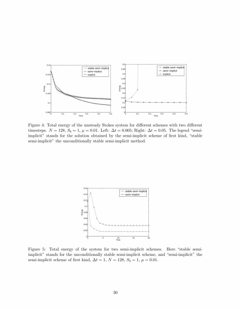
Next, we perform some numerical experiments to test the stability of our semi-implicitschemes for the unsteady Stokes flow. Fig. 4 shows that the energy obtained by the explicitscheme and the semi-implicit scheme of the first kind. We take two different timesteps, 0.005and 0.05. With ∆t = 0.005, the explicit and semi-implicit schemes are all stable, and they givenearly identical results. With ∆t = 0.05, the explicit scheme becomes unstable, but the semi-implicit schemes remain stable. Even if we increase the timestep to ∆t = 1, the semi-implicitmethods are still stable, as we can see from Fig. 5. For the semi-implicit scheme of the firstkind, we have used the Small Scale Decomposition and further simplification of the singularintegral kernel. Therefore, the total energy in our semi-implicit scheme is not guaranteed todecrease monotonically in time. Nonetheless, we observe that the total energy still decreasesin time as is the case for the unconditionally stable semi-implicit scheme. In Fig. 5, we alsoplot the boundary configuration at the final time step, which is an approximate circle.

We remark that the semi-implicit scheme is not unconditionally stable, although its stabilityis much better than the explicit scheme. This is due to the fact that we have used the SmallScale Decomposition and further approximation of the leading order singular integral operatorto simplify the computation of the implicit solution. As we mentioned before, the Small ScaleDecomposition captures only the high frequency contribution to the stiffness, but it does notremove the stiffness of the system induced by the low frequency components of the solution.Thus there is still some mild timestep stability constraint for the semi-implicit scheme. Thetime step has a mild dependence on the elastic coefficient Sb and the viscous coefficient µ. Onthe other hand, our numerical study shows that the time step for the semi-implicit scheme isindependent on the meshsize.

We also compare the performance of our semi-implicit schemes with the explicit scheme. Wedo not compare the performance of our semi-implicit schemes with the fully implicit scheme

29

0 0.1 0.2 0.3 0.4 0.50.095

0.1

0.105

0.11

0.115

0.12

Time

Ene

rgy

stable semi−implicitsemi−implicitexplicit

0 0.1 0.2 0.3 0.4 0.50

0.05

0.1

0.15

0.2

0.25

0.3

0.35

0.4

0.45

0.5

Time

Ene

rgy

stable semi−implicitsemi−implicitexplicit

Figure 4: Total energy of the unsteady Stokes system for different schemes with two differenttimesteps. N = 128, Sb = 1, µ = 0.01. Left: ∆t = 0.005; Right: ∆t = 0.05. The legend “semi-implicit” stands for the solution obtained by the semi-implicit scheme of first kind, “stablesemi-implicit” the unconditionally stable semi-implicit method.

0 5 10 15 200

0.02

0.04

0.06

0.08

0.1

0.12

0.14

0.16

Time

Ene

rgy

stable semi−implicitsemi−implicit

Figure 5: Total energy of the system for two semi-implicit schemes. Here “stable semi-implicit” stands for the unconditionally stable semi-implicit scheme, and “semi-implicit” thesemi-implicit scheme of first kind, ∆t = 1, N = 128, Sb = 1, µ = 0.01.

30

0 0.2 0.4 0.6 0.8 10

0.1

0.2

0.3

0.4

0.5

0.6

0.7

0.8

0.9

1

0 0.2 0.4 0.6 0.8 10

0.1

0.2

0.3

0.4

0.5

0.6

0.7

0.8

0.9

1

Figure 6: Dashed line: the initial boundary configuration; Solid line: the boundary configura-tion after 20 time steps with ∆t = 1, N = 128, Sb = 1, µ = 0.01. Left: the unconditionallystable semi-implicit scheme; Right: the semi-implicit scheme of the first kind.

here because the fully implicit scheme is quite expensive and is not competitive with theexplicit scheme. In order to keep the area loss is no more than 5%, we take ∆t = 1

4 for all ofthe semi-implicit schemes . For the explicit scheme, we take ∆t = 1/64, 1/128, 1/256, 1/512which correspond to the spatial mesh sizes N = 64, 128, 256, 512 respectively, when µ = 0.05.When µ = 0.01 and 0.005, the time step is set to be ∆t = 1/128, 1/256, 1/512, 1/1024 andt = 1/256, 1/512, 1/1024, 1/2048. These time steps are the largest ones we can take to keep thestability. We compute the solution up to T = 2. The results are documented in Table 2. Wecan clearly see that the semi-implicit scheme of the first kind gives a significant improvementover the explicit scheme. The cost for the semi-implicit scheme of the second kind is higherthan that for the semi-implicit scheme of the first kind. This is because we need to solvefor a linear system at each time step for the semi-implicit scheme of the second kind. Thecost increases as the number of the spatial grid points increases. The semi-implicit schemeof the second kind and the unconditionally stable semi-implicit scheme both need to solve alinear system at each time step. Their complexity are same, both are O(N 2

b ). But for theunconditionally stable semi-implicit scheme, the scaling constant in front of N 2

b is much largerthan the semi-implicit scheme of the second kind. The reason is that the cost of computingthe coefficient matrix of the linear system for the unconditionally stable semi-implicit schemeis much higher. As we can see from Table 2, the unconditionally stable semi-implicit scheme(labeled as s,s,i) is still quite expensive compared with our semi-implicit schemes that use theSmall Scale Decomposition. For µ = 0.05, the unconditionally stable semi-implicit scheme iseven more expensive compared with the explicit scheme. Although the unconditionally stablesemi-implicit scheme is slightly faster than the explicit scheme for smaller µ, the semi-implicitscheme (labeled as s,i,1) which uses SSD to further simply the singular integral kernel gives amuch more efficient algorithm. It gives a factor of 242 times speed-up over the explicit schemein the case of µ = 0.005 and N = 512.

31

N µ = 0.05 µ = 0.01 µ = 0.005exp s,i 1 s,i 2 s,s,i exp s,i 1 s,i 2 s,s,i exp s,i 1 s,i 2 s,s,i

64 1.8 0.5 4 11 3.3 0.5 4 12 6.6 0.5 4 12

128 9 1 10 48 18 0.9 10 47 35 0.9 10 48

256 58 2.4 25 229 116 2.4 25 228 236 2.4 25 226

512 738 12 99 980 1461 12 98 982 2910 12 98 977

Table 2: Execution times for each computation in seconds. The legends are defined as follows:“exp” stands for the explicit scheme, “s,i1” the semi-implicit scheme of the first kind, “s,i2”the semi-implicit scheme of the second kind, “s,s,i” the unconditionally stable semi-implicitscheme.

7.4 Second order semi-implicit scheme for the unsteady Stokes flow

In this subsection, we perform numerical experiments to test the convergence rate and thestability property of our second order semi-implicit scheme. To check the convergence rate intime, we set N = 256 and vary the time step in powers of 2 from 1

16 to 1128 . When µ = 0.005,

the solution becomes more singular. In order to fully resolve the spatial solution, we increasethe spatial resolution to N = 512. Following [23], we compute the time discretization error attime t as follows:

eT (u;∆t) = ‖u(T ;∆t) − u(T ;∆t/2)‖l2 . (209)

For a vector field u(x) = (u1(x), u2(x)) defined on the Cartesian grid with xi = ih, yj = jh,the discrete l2 norm is defined as follows

‖u‖l2 =

∑

i,j

(u2

1(xi, yj) + u22(xi, yj)

)h2

1

2

. (210)

Similarly, the discrete l2 norm for a vector field w(α) = (w1(α), w2(α)) defined on the interfaceΓ is defined below:

‖w‖l2 =

(∑

i

(w2

1(αi) + w22(αi)

)∆α

) 1

2

. (211)

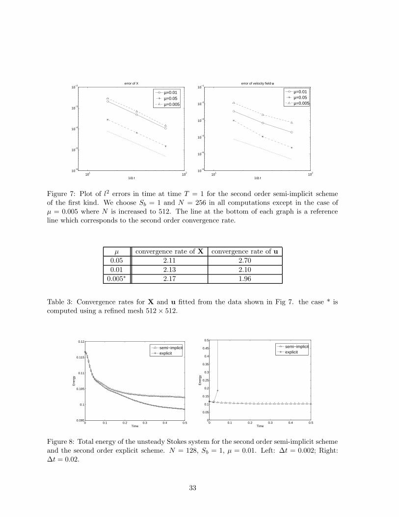
We compute the solution up to T = 1 and evaluate the convergence rate based on the numericalsolution at T = 1 with different temporal resolutions. The results are shown in Fig. 7 andTable 3. As we can see, the convergence rate is approximately second order.

Next we check the stability of the second order semi-implicit scheme. Fig 8 shows thatthe total energy for the second order explicit and second order semi-implicit schemes withdifferent timesteps 0.002 and 0.02. We choose the same second order explicit scheme that wasused in [13]. With ∆t = 0.002, both the explicit and semi-implicit schemes are stable andthey give nearly identical results. With ∆t = 0.02, the explicit scheme becomes unstable, butthe semi-implicit scheme is still stable. The stability restriction of the semi-implicit scheme isfar less severe than the corresponding explicit scheme. Our numerical study also shows that

32

101

102

10−6

10−5

10−4

10−3

10−2

1/∆ t

error of X

µ=0.01µ=0.05µ=0.005

101

102

10−6

10−5

10−4

10−3

10−2

10−1

1/∆ t

error of velocity field u

µ=0.01µ=0.05µ=0.005

Figure 7: Plot of l2 errors in time at time T = 1 for the second order semi-implicit schemeof the first kind. We choose Sb = 1 and N = 256 in all computations except in the case ofµ = 0.005 where N is increased to 512. The line at the bottom of each graph is a referenceline which corresponds to the second order convergence rate.

µ convergence rate of X convergence rate of u

0.05 2.11 2.70

0.01 2.13 2.10

0.005∗ 2.17 1.96

Table 3: Convergence rates for X and u fitted from the data shown in Fig 7. the case * iscomputed using a refined mesh 512 × 512.

0 0.1 0.2 0.3 0.4 0.50.095

0.1

0.105

0.11

0.115

0.12

Time

Ene

rgy

semi−implicitexplicit

0 0.1 0.2 0.3 0.4 0.50

0.05

0.1

0.15

0.2

0.25

0.3

0.35

0.4

0.45

0.5

Time

Ene

rgy

semi−implicitexplicit

Figure 8: Total energy of the unsteady Stokes system for the second order semi-implicit schemeand the second order explicit scheme. N = 128, Sb = 1, µ = 0.01. Left: ∆t = 0.002; Right:∆t = 0.02.

33

N µ = 0.05 µ = 0.01 µ = 0.005explicit semi-implicit explicit semi-implicit explicit semi-implicit

64 7 0.8 7 0.8 7 0.8

128 37 1.6 38 1.6 38 1.6

256 249 4.4 504 4.6 506 4.5

512 3088 24 6182 25 6200 25

Table 4: Execution time for each computation in seconds. Here “explicit” stands for the secondorder explicit scheme and “semi-implicit” the second order semi-implicit scheme.

the time step for the semi-implicit scheme is independent on the meshsize while the explicitscheme requires finer time step as the spatial mesh is refined.

Finally, we compare the performance of our second order semi-implicit scheme with thatof the second order explicit scheme. As before, in order to keep the accuracy with 5%,we take ∆t = 1

4 for our semi-implicit schemes. For the explicit scheme, we take ∆t =1/128, 1/256, 1/512, 1/1024 which correspond to the spatial mesh sizes N = 64, 128, 256, 512respectively, when µ = 0.05. When µ = 0.01 and 0.005, the time step is set to be ∆t =1/128, 1/256, 1/1024, 1/2048. These time steps are the largest ones that we can take to keepthe stability of the explicit scheme. We compute the solution up to T = 2. The result is shownin Table 4. Again, we observe the same qualitative behavior as the first order schemes wereported earlier.

8 Concluding Remarks

In this paper, we have developed several efficient semi-implicit immersed boundary methodsfor solving the immersed boundary problem for the steady and unsteady Stokes equations.The immersed boundary method has emerged as one of the most useful numerical methodsin computing fluid structure interaction, and has found numerous applications. But it alsosuffers from the severe time step stability limitation due to the stiffness of the elastic force.Guided by our stability analysis, we have developed several efficient semi-implicit schemeswhich remove the stiffness of the immersed boundary method. We have demonstrated bothanalytically and computationally that our semi-implicit schemes have much better stabilityproperty than the explicit scheme. More importantly, unlike most existing implicit or semi-implicit schemes, our semi-implicit schemes can be implemented very efficiently. In fact, oursemi-implicit scheme of the first kind has a computational cost that is essentially the same asthat of an explicit scheme in each time step, but with a much better stability property. Thesaving in the computational cost is quite substantial. We have demonstrated this improvedstability for a range of parameters and numerical resolutions. Our computational results showthat the larger the spatial resolution is, the bigger the computational saving our semi-implicitschemes can offer. Thus the semi-implicit schemes we develop in this paper provide an effectivealternative discretization to the explicit method.

One of the essential steps in developing our semi-implicit schemes is to obtain an uncondi-tionally stable semi-implicit discretization of the immersed boundary problem. This providesus with a building block to construct our efficient semi-implicit schemes. There are two im-

34

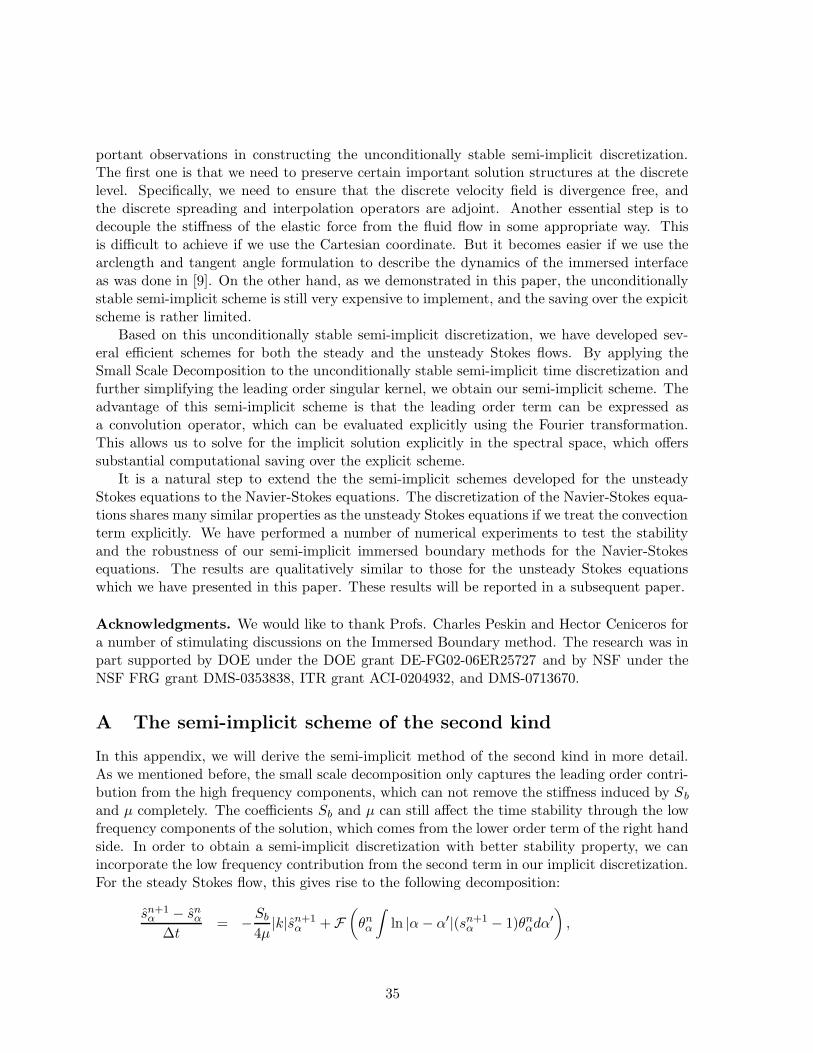
portant observations in constructing the unconditionally stable semi-implicit discretization.The first one is that we need to preserve certain important solution structures at the discretelevel. Specifically, we need to ensure that the discrete velocity field is divergence free, andthe discrete spreading and interpolation operators are adjoint. Another essential step is todecouple the stiffness of the elastic force from the fluid flow in some appropriate way. Thisis difficult to achieve if we use the Cartesian coordinate. But it becomes easier if we use thearclength and tangent angle formulation to describe the dynamics of the immersed interfaceas was done in [9]. On the other hand, as we demonstrated in this paper, the unconditionallystable semi-implicit scheme is still very expensive to implement, and the saving over the expicitscheme is rather limited.

Based on this unconditionally stable semi-implicit discretization, we have developed sev-eral efficient schemes for both the steady and the unsteady Stokes flows. By applying theSmall Scale Decomposition to the unconditionally stable semi-implicit time discretization andfurther simplifying the leading order singular kernel, we obtain our semi-implicit scheme. Theadvantage of this semi-implicit scheme is that the leading order term can be expressed asa convolution operator, which can be evaluated explicitly using the Fourier transformation.This allows us to solve for the implicit solution explicitly in the spectral space, which offerssubstantial computational saving over the explicit scheme.

It is a natural step to extend the the semi-implicit schemes developed for the unsteadyStokes equations to the Navier-Stokes equations. The discretization of the Navier-Stokes equa-tions shares many similar properties as the unsteady Stokes equations if we treat the convectionterm explicitly. We have performed a number of numerical experiments to test the stabilityand the robustness of our semi-implicit immersed boundary methods for the Navier-Stokesequations. The results are qualitatively similar to those for the unsteady Stokes equationswhich we have presented in this paper. These results will be reported in a subsequent paper.

Acknowledgments. We would like to thank Profs. Charles Peskin and Hector Ceniceros fora number of stimulating discussions on the Immersed Boundary method. The research was inpart supported by DOE under the DOE grant DE-FG02-06ER25727 and by NSF under theNSF FRG grant DMS-0353838, ITR grant ACI-0204932, and DMS-0713670.

A The semi-implicit scheme of the second kind

In this appendix, we will derive the semi-implicit method of the second kind in more detail.As we mentioned before, the small scale decomposition only captures the leading order contri-bution from the high frequency components, which can not remove the stiffness induced by Sb

and µ completely. The coefficients Sb and µ can still affect the time stability through the lowfrequency components of the solution, which comes from the lower order term of the right handside. In order to obtain a semi-implicit discretization with better stability property, we canincorporate the low frequency contribution from the second term in our implicit discretization.For the steady Stokes flow, this gives rise to the following decomposition:

sn+1α − sn

α

∆t= −Sb

4µ|k|sn+1

α + F(θnα

∫ln |α− α′|(sn+1

α − 1)θnαdα

′

),

35

+

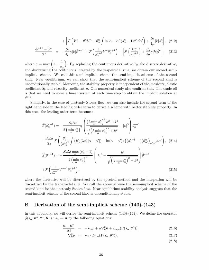
[F(V n

α − θnαU

n − θnα

∫ln |α− α′|(sn

α − 1)θnαdα

′

)+Sb

4µ|k|sn

α

], (212)

φn+1 − φn

∆t= −Sb

4µγ|k|φn+1 + F

(1

sn+1α

V nθn+1α

)+

[F(Un

α

sn+1α

)+Sb

4µγ|k|φn

], (213)

where γ = maxα

(1 − 1

sα

). By replacing the continuous derivative by the discrete derivative,

and discretizing the continuous integral by the trapezoidal rule, we obtain our second semi-implicit scheme. We call this semi-implicit scheme the semi-implicit scheme of the secondkind. Near equilibrium, we can show that the semi-implicit scheme of the second kind isunconditionally stable. Moreover, the stability property is independent of the meshsize, elasticcoefficient Sb and viscosity coefficient µ. Our numerical study also confirms this. The trade-offis that we need to solve a linear system at each time step to obtain the implicit solution attn+1.

Similarly, in the case of unsteady Stokes flow, we can also include the second term of theright hand side in the leading order term to derive a scheme with better stability property. Inthis case, the leading order term becomes:

T (sn+1α ) = − Sb∆t

2(min

αsnα

)2

(λmin

αsnα

)2k2 + k4

√(λmin

αsnα

)2+ k2

− |k|3

s

n+1α

−Sb∆t

2πF(

θnα

(snα)2

∫ (K0(λs

nα|α− α′|) − ln(α− α′)

) ((sn+1

α − 1)θnα′

)α′α′

dα′

), (214)

S(θn+1) = −Sb∆tmax

α(sn

α − 1)

2(min

αsnα

)2

|k|3 −

k4

√(λmin

αsnα

)2+ k2

θ

n+1

+F(

1

sn+1α

V n+1θn+1α

), (215)

where the derivative will be discretized by the spectral method and the integration will bediscretized by the trapezoidal rule. We call the above scheme the semi-implicit scheme of thesecond kind for the unsteady Stokes flow. Near equilibrium stability analysis suggests that thesemi-implicit scheme of the second kind is unconditionally stable.

B Derivation of the semi-implicit scheme (140)-(143)

In this appendix, we will derive the semi-implicit scheme (140)-(143). We define the operatorG(sα;un, θn,Xn) : sα → u by the following equations:

u − un

∆t= −∇hp+ µ∇2

hu + Lh,n(F(sα, θn)), (216)

∇2hp = ∇h · Lh,n(F(sα, θ

n)). (217)

(218)

36

Given sα, we obtain u by solving above equations. From the definition of operator G, we have

un+1 = G(sn+1α ;un, θn,Xn),

u∗,n+1 = G(snα;un, θn,Xn),

where u∗,n+1 is calculated from equations (140)-(141).Then the equation of sα can be rewritten as

sn+1α − sn

α

∆t= D∆αV

n+1 −D∆αθnUn+1

= D∆α

(L∗

h,n(un+1) · τ n)−D∆αθ

n(L∗

h,n(un+1 · nn))

= D∆α

(L∗

h,n

(G(sn+1

α ;un, θn,Xn))· τ n

)

−D∆αθn(L∗

h,n

(G(sn+1

α ;un, θn,Xn))· nn

)

≡ R(sn+1α ;un, θn,Xn). (219)

Using the small scale decomposition, we get

R(sn+1α ;un, θn,Xn) ∼ T (sn+1

α ). (220)

By treating the leading order term implicitly, we obtain our semi-implicit method as follows:

sn+1α − sn

α

∆t= T (sn+1

α ) + (R(snα;un, θn,Xn) − T (sn

α))

= T (sn+1α ) +D∆α

(L∗

h,n (G(snα;un, θn,Xn)) · τn

)

−D∆αθn(L∗

h,n (G(snα;un, θn,Xn)) · nn

)− T (sn

α)

= T (sn+1α ) +D∆α

(L∗

h,n(u∗,n+1) · τn)−D∆αθ

n(L∗

h,n(u∗,n+1) · nn)

−T (snα)

= T (sn+1α ) +

(D∆αV

∗,n+1 −D∆αθnU∗,n+1 − T (sn

α)). (221)

This is exactly our semi-implicit scheme (134).In the steady Stokes case, we can define the operator G(sα;un, θn,Xn) : sα → u similarly:

0 = −∇hp+ µ∇2hu + Lh,n(F(sα, θ

n)), (222)

∇2hp = ∇h · Lh,n(F(sα, θ

n)). (223)

In this case, we have

G(snα;un, θn,Xn) = un.

Thus, the semi-implicit scheme becomes

sn+1α − sn

α

∆t= T (sn+1

α ) + (D∆αVn −D∆αθ

nUn − T (snα)) . (224)

37

C The derivation of the Fourier transform of K0

In this appendix, we derive the the Fourier transform of K0, which is given in (144). By thedefinition of the Fourier transform, we have

F(

1

π

∫ +∞

−∞K0(β|α− α′|)f(α′)dα′

)

=1

π

∫ +∞

−∞

(∫ +∞

−∞K0(β|α− α′|)f(α′)dα′

)e−ikαdα

=1

π

∫ +∞

−∞

∫ +∞

−∞K0(β|α− α′|)f(α′)e−ikαdα′dα

=1

π

∫ +∞

−∞

∫ +∞

−∞K0(β|α− α′|)f(α′)e−ik(α−α′)e−ikα′

dα′d(α− α′)

=1

π

∫ +∞

−∞

(∫ +∞

−∞K0(β|α− α′|)e−ik(α−α′)d(α − α′)

)f(α′)e−ikα′

dα′

=

∫ +∞

−∞

f(α′)√β2 + k2

e−ikα′

dα′ =f(k)√β2 + k2

, (225)

where F(f(α))(k) =

∫ +∞

−∞f(α)eikαdα is the Fourier transform. In the calculation above, we

have used the expression of the Bessel function (p 376, [1])

K0(x) =

∫ +∞

0

cos(tx)√1 + t2

dt, (226)

and the identity below:

∫ +∞

−∞K0(β|x|)e−ikxdx =

∫ +∞

−∞

∫ +∞

0

cos(βtx)√1 + t2

e−ikxdtdx

=1

2

∫ +∞

−∞

∫ +∞

−∞

cos(βtx)√1 + t2

e−ikxdtdx

=1

2

∫ +∞

−∞

∫ +∞

−∞

eiβtx

√1 + t2

e−ikxdtdx

=1

2

∫ +∞

−∞

∫ +∞

−∞

ei(βt−k)x

√1 + t2

dtdx

= π

∫ +∞

−∞

δ(βt − k)√1 + t2

dt =π√

β2 + k2. (227)

This proves (144).

References

[1] M. Abramowitz and I. A. Stegun, Modified Bessel Functions I and K, New York:Dover, 9th printing (1972).

38

[2] R. P. Beyer, A computational model of the cochlea using the immersed boundary method,J. Comput. Phys., 98(1992) pp. 145-162

[3] R. Cortez, N. Cowen, R. Dillon, L. J. Fauci, Simulation of swimming organisms: Couplinginternal mechanics with external fluid dynamics, Comput. Sci. Eng. 6 (2004), pp. 38-45

[4] H. D. Ceniceros, A. M. Roma, Study of the long-time dynamics of viscous vortex sheetwith a fully adaptive nonstiff method, Physics of Fluid 16 (2004), pp 4285-4318

[5] L. Fauci and C. S. Peskin, A computational model of aquatic animal locomotion, J. Com-put. Phys., 77 (1988), pp. 85-108

[6] L. J. Fauci, Interaction of oscillating filaments - A computational study, J. Comput. Phys,86(1990) pp. 294-313

[7] A. L. Fogelson, A mathematical model and numerical methods for studying platelet adhe-sion and aggregation during blood clotting, J. Comput. Phys., 56 (1984), pp. 111-134

[8] E. Givelberg, Modeling elastic shells immersed in fluid, PhD thesis (1997), Courant Insti-tute of Mathematical Sciences, New York University

[9] T. Y. Hou, J. Lowengrub and M. Shelley, Removing the stiffness from interfacial flowswith surface tension, J. Comput Phys., 114 (1994), pp. 312-338.

[10] T. Y. Hou, J. Lowengrub and M. Shelley, The long-time motion of vortex sheets withsurface tension, Phys. Fluid A, 9 (1997), pp. 1933-1954.

[11] M. Hopkins and L. J. Fauci, A computational model of the collective fluid dynamics ofmotile microorganisms, J. Fluid Mech., 455(2002), pp. 149-174

[12] E. N. Jung and C. S. Peskin, Two-dimensional simulations of valveless pumping using theimmersed boundary method, SIAM J. Sci. Comput. 23 (2001), pp. 19-45.

[13] M. C. Lai and C. S. Peskin. An immersed boundary method with formal second orderaccuracy and reduced numerical viscosity, J. Comput. Phys., 160 (2000), pp. 705-719

[14] R. J. LeVeque and Z. Li, Immersed Interface methods for Stokes flow with elastic bound-aries or surface tension, SIAM J. Sci. Comput. 18 (1997), pp. 709-735.

[15] A. A. Mayo and C. S. Peskin, An implicit numerical method for fluid dynamics problemswith immersed elastic boundaries, Contemporary Mathematics, 141 (1993), pp. 261-277.

[16] D. M. McQueen, C. S. Peskin, and E. L. Yellin, Fluid dynamics of the mitral valve:Physiological aspects of a mathematical model, Amer. J. Physiol. 242 (1982), pp. H1095-H1110.

[17] D. M. McQueen and C. S. Peskin, Computer assisted design of pivoting-disc prostheticmitral valves, J. Thorac. Cardiovasc. Surg., 86 (1983), pp. 126-135.

[18] D. M. McQueen and C. S. Peskin, Computer assisted design of butterfly bileaflet valvesfor mitral position, Scand. J. Thorac. Cardiovasc. Surg., 19 (1985), pp. 139-148.

39

[19] D. M. McQueen and C. S. Peskin, A three-dimensional computational method for bloodflow in the heart: (II) Contractile fibers, J. Comput. Phys., 82 (1989), pp. 289-297.

[20] D. M. McQueen and C. S. Peskin, Heart simulation by an immersed boundary methodwith formal second order accuracy and reduced viscosity. In Mechanics for a New Millen-nium, Proceedings of the International Conference on Theoretical and Applied mechanics(ICTAM) 2000, Kluwer Academic Publishers.

[21] L. A. Miller and C. S. Peskin, When vortices stick: and aerodynamic transition in tinyinsects, J. Exp. Biol., 207(2004), pp. 3073-3088

[22] L. A. Miller and C. S. Peskin, A computational fluid dynamics of ’clap and fling’ in smallinsects, J. Exp. Biol., 208(2005), pp. 195-212

[23] Y. Mori and C. S. Peskin, A second order implicit Immersed Boundary method with bound-ary mass. Preprint, 2007, submitted to Computational Mechanics.

[24] E. P. Newren, A. L. Fogelson, R. D. Guy and R. M. Kirby Unconditionally stable discretiza-tions of the immersed boundary equations, J. Comput. Phys., 222 (2007), pp. 702-719.

[25] C. S. Peskin, Numerical study of blood flow in the heart, J. Comput. Phys., 25 (1977), pp.220-252.

[26] C. S. Peskin and D. M. McQueen , A three-dimensional computational method for bloodflow in the heart: (I) Immersed elastic fibers in a viscous incompressible fluid, J. Comput.Phys., 81 (1989), pp. 372-405.

[27] C. S. Peskin, The immersed boundary method, Acta Numerica, 11 (2002), pp. 479-517

[28] C. Pozrikidis, Boundary Integral and Singularity Methods for Linearized Vis-

cous Flow, Cambridge University Press, 1992.

[29] M. E. Rosar and C. S. Peskin, Fluid flow in collapsible elastic tubes: a three-dimensionalnumerical model, New York J. Math. 7 (2001), pp. 281-302.

[30] J. M. Stockie and B. R. Wetton, Stability analysis for the immersed fiber problem, SIAMJ. Appl. Math, 55 (1995), pp. 1577-1591.

[31] , J. M. Stockie and S. I. Green, Simulating the motion of flexible pulp fibers using theimmersed boundary method, J. Comput. Phys., 147(1998), pp. 147-165

[32] J. M. Stockie and B. R. Wetton, Analysis of stiffness in the Immersed Boundary methodand implications for time-stepping schemes, J. Comput Phys, 154 (1999), pp. 41-64.

[33] C. Tu and C. S Peskin, Stability and instability in the computation of flows with movingimmersed boundaries: A comparison of three methods, SIAM J. Sci. Stat. Comput, 13

(1992), pp. 1361-1376.

[34] N. T. Wang and A. L. Fogelson, Computational methods or continuum models of plateletaggregation, J. Comput. Phys., 151 (1999), pp. 649-675.

40

[35] L. Zhu and C. S. Peskin, Simulation of a flexible flapping filament in a flowing soap filmby the immersed boundary method, J. Comput. Phys., 179(2002), pp. 452-468

[36] J. Zhu, X. Chen, T. Y. Hou, An efficient boundary integral method for the Mullins-Sekerkaproblem, J Comput Phys., 127 (1996), pp. 246-267.

41