Naval Research LaboratoryStennis Space Center, MS 39529-5004

NRL/MR/7330--16-9684

Approved for public release; distribution is unlimited.

Remote Sensing Systems to Detect andAnalyze Oil Spills on the U.S. OuterContinental Shelf — A State of the ArtAssessment

Derek Burrage Sonia gallegoS Joel WeSSon richarD goulD richarD crout Sean Mccarthy

Ocean Sciences Branch Oceanography Division

August 18, 2016

i

REPORT DOCUMENTATION PAGE Form ApprovedOMB No. 0704-0188

3. DATES COVERED (From - To)

Standard Form 298 (Rev. 8-98)Prescribed by ANSI Std. Z39.18

Public reporting burden for this collection of information is estimated to average 1 hour per response, including the time for reviewing instructions, searching existing data sources, gathering and maintaining the data needed, and completing and reviewing this collection of information. Send comments regarding this burden estimate or any other aspect of this collection of information, including suggestions for reducing this burden to Department of Defense, Washington Headquarters Services, Directorate for Information Operations and Reports (0704-0188), 1215 Jefferson Davis Highway, Suite 1204, Arlington, VA 22202-4302. Respondents should be aware that notwithstanding any other provision of law, no person shall be subject to any penalty for failing to comply with a collection of information if it does not display a currently valid OMB control number. PLEASE DO NOT RETURN YOUR FORM TO THE ABOVE ADDRESS.

5a. CONTRACT NUMBER

5b. GRANT NUMBER

5c. PROGRAM ELEMENT NUMBER

5d. PROJECT NUMBER

5e. TASK NUMBER

5f. WORK UNIT NUMBER

2. REPORT TYPE1. REPORT DATE (DD-MM-YYYY)

4. TITLE AND SUBTITLE

6. AUTHOR(S)

8. PERFORMING ORGANIZATION REPORT NUMBER

7. PERFORMING ORGANIZATION NAME(S) AND ADDRESS(ES)

10. SPONSOR / MONITOR’S ACRONYM(S)9. SPONSORING / MONITORING AGENCY NAME(S) AND ADDRESS(ES)

11. SPONSOR / MONITOR’S REPORT NUMBER(S)

12. DISTRIBUTION / AVAILABILITY STATEMENT

13. SUPPLEMENTARY NOTES

14. ABSTRACT

15. SUBJECT TERMS

16. SECURITY CLASSIFICATION OF:

a. REPORT

19a. NAME OF RESPONSIBLE PERSON

19b. TELEPHONE NUMBER (include areacode)

b. ABSTRACT c. THIS PAGE

18. NUMBEROF PAGES

17. LIMITATIONOF ABSTRACT

Remote Sensing Systems to Detect and Analyze Oil Spills on the U.S. Outer Continental Shelf — A State of the Art Assessment

Derek Burrage, Sonia Gallegos, Joel Wesson, Richard Gould,Richard Crout, and Sean McCarthy

Naval Research LaboratoryOceanography DivisionStennis Space Center, MS 39529-5004

NRL/MR/7330--16-9684

Approved for public release; distribution is unlimited.

UnclassifiedUnlimited

UnclassifiedUnlimited

UnclassifiedUnlimited

UnclassifiedUnlimited

109

Derek Burrage

228-688-5182

This technical report describes the assessment and evaluation of the capabilities and limitations of current oil spill detection and analysis systems for use in offshore oil and gas operations on the U.S. outer continental shelf. The assessment considers a range of operational and experimental remote sensing systems that are currently in use, or under development, and their practicality under different oil spill scenarios. The evaluation considers the suitability for intended use of the sensors and their strengths and limitations. It also considers the hardware and operational requirements, platform mounting and delivery options, and costs. Other project deliverables, which complement this technical report, include the final report, an interactive spreadsheet system incorporating a searchable database to aid in selecting appropriate technologies and sensors for a variety of oil spill scenarios, a supporting user guide, and a journal article detailing the methodology and findings of the project. A browser-based sensor selection tool (or “demo”) with a graphical user interface is also provided as a prototype for a web-based version that could be developed in a future project.

18-08-2016 Memorandum Report

Oil spillScenario Sensor performance

DatabaseClassification Interactive tool

Decision rule

73-1B58-04-5

Bureau of Safety and Environmental Enforcement381 Elden Street, HE 2306Herndon, VA 20170

BSEE

iii

Remote Sensing Systems to Detect and Analyze Oil Spills on the US Outer Continental Shelf – A State of the Art Assessment

Technical Report

12 Apr, 2016

Authors: Derek Burrage (P.I.)*, Sonia Gallegos, Joel Wesson, Richard Gould,

Richard Crout and Sean McCarthy.

Ocean Sciences Branch, Naval Research Laboratory, Stennis Space Center, 39529, MS, USA.

Acknowledgement

This study was funded by the U.S. Department of the Interior, Bureau of Safety and Environmental Enforcement through Interagency Agreement E14PG00058 with the Naval Research Laboratory.

Caveat

This technical report has been reviewed by the BSEE and approved for publication. Approval does not signify that the contents necessarily reflect the views and policies of the BSEE, nor does mention of the trade names or commercial products constitute endorsement or recommendation for use.

*Contact Phone: (228) 688 5241 (W) (985) 285 9563 (C) Email: derek.burrage@nrlssc.navy.mil

______________________________________________________________________________________

BAA for Research on Oil Spill Response Operations in the U.S. OCS

BSEE Project Number: E14PS00011

Topic: Oil Spill Detection and Analysis Using Remote Sensing Technologies.

v

Table of Contents Introduction ................................................................................................................................................................................................ 1

Technical Approach ................................................................................................................................................................................. 3

Study Outline .......................................................................................................................................................................................... 4

Methodology........................................................................................................................................................................................... 5

Part 1: Sensor Evaluation Criteria................................................................................................................................................................ 9

Sensor Classification ............................................................................................................................................................................... 9

Optical Methods ............................................................................................................................................................................... 11

Microwave Methods......................................................................................................................................................................... 12

Oil Spill Remote Sensing Requirements ................................................................................................................................................ 12

Sensor Evaluation ................................................................................................................................................................................. 13

Sensor Specifications ............................................................................................................................................................................ 15

Sensor Identity .................................................................................................................................................................................. 17

Instrument Costs and Data Plan ....................................................................................................................................................... 18

Technology ....................................................................................................................................................................................... 18

Measurement Parameters ................................................................................................................................................................ 18

Electro-Magnetic Spectrum Properties ............................................................................................................................................ 19

Sensor Performance Criteria ................................................................................................................................................................. 20

Spill Sensing Capability ..................................................................................................................................................................... 22

Data Accessibility .............................................................................................................................................................................. 23

Hardware Accessibility ..................................................................................................................................................................... 24

Instrument Costs and Data Plan ....................................................................................................................................................... 25

Part 2: Specification of Scenarios .............................................................................................................................................................. 27

Employing Spill Scenarios...................................................................................................................................................................... 27

Scenario Definition................................................................................................................................................................................ 28

Scenario Identification Group ........................................................................................................................................................... 31

Scenario Analysis Group ................................................................................................................................................................... 32

Spill Location and Proximity to Land Group ..................................................................................................................................... 32

Spill Type and Conditions Group ...................................................................................................................................................... 32

Initial Release Group ........................................................................................................................................................................ 32

Estimated Spill Size Group ................................................................................................................................................................ 32

Oil Type and Condition Group .......................................................................................................................................................... 33

vi

Ocean Met Conditions and Water Properties Group ....................................................................................................................... 33

Observer Constraints Group ............................................................................................................................................................. 33

Application of Oil Spill Weathering and Trajectory Models .................................................................................................................. 33

NOAA ADIOS Weathering Model ...................................................................................................................................................... 34

NOAA GNOME Oil Spill Advection Model ......................................................................................................................................... 34

Model-based Scenario Development ............................................................................................................................................... 35

Part 3: Sensor Selection and Evaluation .................................................................................................................................................... 37

The Sensor Survey ................................................................................................................................................................................. 37

The IDAOS Excel Workbook .................................................................................................................................................................. 37

Caveats Regarding Spreadsheet Function and Use .......................................................................................................................... 38

Instrument Performance .................................................................................................................................................................. 39

Suitability for Intended Use .............................................................................................................................................................. 39

Part 4: Preferred Sensors .......................................................................................................................................................................... 42

Sensor Selection .................................................................................................................................................................................... 42

Sensor Performance by Category and Class ......................................................................................................................................... 43

Spill Types and Representative Examples ............................................................................................................................................. 45

Sensor Deployment Modes ................................................................................................................................................................... 48

Sensor Application Types ...................................................................................................................................................................... 48

Sensor Platform Types .......................................................................................................................................................................... 50

Deployment Mode Descriptions ........................................................................................................................................................... 53

Part 5: Results and Recommendations ..................................................................................................................................................... 63

Sensor Selection .................................................................................................................................................................................... 63

Excel Spreadsheet-Based Sensor Selection Tool ................................................................................................................................... 65

A Prototype Internet-Based Sensor Selection Tool............................................................................................................................... 67

Desirable Characteristics of a Comprehensive Sensor Selection Tool .................................................................................................. 69

Technical Recommendations ................................................................................................................................................................ 70

Appendix: Excel Spreadsheet User Guide ................................................................................................................................................. 72

The IDAOS Excel Spreadsheet ............................................................................................................................................................... 72

Spreadsheet Structure ...................................................................................................................................................................... 72

Decision Rules ................................................................................................................................................................................... 81

Using the Spreadsheet ...................................................................................................................................................................... 94

References .......................................................................................................................................................................................... 102

E-1

Executive Summary

This technical report describes the assessment and evaluation of the capabilities and limitations of current oil spill detection and analysis systems for use in offshore oil and gas operations on the US outer continental shelf. The assessment considers a range of operational and experimental remote sensing systems that are currently in use, or under development, and their practicality under different oil spill scenarios. The evaluation considers the suitability for intended use of the sensors and their strengths and limitations. It also considers the hardware and operational requirements, platform mounting and delivery options, and costs. Other project deliverables, which complement this technical report, include the final report, an interactive spreadsheet system incorporating a searchable data base to aid in selecting appropriate technologies and sensors for a variety of oil spill scenarios, a supporting user guide, and a journal article detailing the methodology and findings of the project. A browser-based sensor selection tool (or ‘demo’) with a graphical user interface, is also provided as a prototype for a web-based version that could be developed in a future project.

Introduction Efficient and rapid detection of oil spills that occur over the continental shelf is vitally important for a host of societal, environmental, economic and public safety reasons. However, the variety of spill sizes and types, coupled with the dynamic environment and rapidly evolving physical and chemical characteristics of a spill and changing weather conditions, makes detection and analysis using remote sensing methods challenging.

This assessment is motivated by the need for oil spill response planners and operators to have up-to-date information on available and developing technologies and systems for oil spill detection and analysis. These systems must meet their needs in a variety of spill scenarios, and under various observational conditions (including the expected meteorological and oceanographic conditions and, if known, the disposition and physico-chemical condition of the oil), as well as logistical and resource constraints. A comprehensive review of the technology available 20+ years ago (Fingas, 1991) as part of the Technology Assessment Program (TAP) project # 154, provided a useful reference for assessing more recent progress. That review was released soon after the 1989 Exxon Valdez oil spill in Prince William Sound, Alaska. It considered both optical and microwave technologies and has been updated several times (most recently in Fingas and Brown, 2014). Other reviews published in the intervening period include Goodman (1994), Brown and Fingas (2003), Brekke and Solberg (2005) and Jha et al (2008). Some of these were applied to particular geographic conditions or regions. Puestow et al., 2013, which focused on spill detection and mapping in low visibility and ice under conditions found in the Arctic, could also be applicable to the Alaskan shelf. The review by Leifer et al. (2012), which surveyed the sensors deployed during the 2010 BP Deep Water Horizon (DWH) Oil Spill in the Gulf of Mexico, focused primarily on optical technologies, but also discussed active radar systems.

The planning guidance on remote sensing to support oil spill response provided in the American Petroleum Institute (API, 2013) surveyed the principal types of remote sensing technology that are appropriate for this purpose. Using a primary classification based on Visual Observation, Active/Passive sensors and Multi-band and Multi-sensor integration, the report advocated sensor selection based on oil spill response mission goals and prevailing conditions. For each sensor type, the report addressed questions concerning its nature and function, effectiveness, Pros and Cons, and available instrument platforms. The report was supported by a set of spreadsheets containing information on Current Research and Emerging Trends, with multiple entries under the topics Peer-reviewed Papers, Lessons learned from Recent Spills and Oil Spill Research and Development Programs. However, technical, operational, cost, mounting and other details of particular sensors or sensor suites were not provided.

Two recent reports assessing surface surveillance capabilities for oil spill response using satellite and airborne remote sensing by Partington (2014a,b) supplement and expand on the many reviews and comparisons of remote sensing instrumentation for oil spill response that have been prepared over the decades. As in the ________________Manuscript approved June 9, 2016.

1

Introduction 2

previously published reviews, they contain similar information with respect to the major remote sensing technology classes and their capabilities. However, they are generally more comprehensive and up to date. In some areas they contain substantive new and useful information that we draw on in this work e.g. in the satellite report (Partington, 2014a), there is a detailed analysis of time delays in obtaining data (ordering lead times and data latencies). This is a topic that is undergoing such rapid change that it is virtually impossible to keep a hard copy report updated on a useful time scale. Another area addressed, in the airborne report (Partington, 2014b), is the likely increase in deployment of remote sensing equipment on Unmanned Aerial Vehicles, UAVs, a.k.a. Unmanned Aerial Systems (UAS). Indeed, one of the conclusions of the airborne report is "Given this rapid pace of change, there is a strong case for the information in this report to be updated on a regular basis, perhaps every year." This highlights the key problem of relying exclusively on static reporting to address the requirements of the highly dynamic environmental assessment and enforcement field of oil spill response, and motivated us to develop a more dynamic approach. Hence we have placed the sensor information that we have acquired from various reference sources into more readily updated database form. We have also provided automated decision making tools in the form of an Excel spreadsheet system (along with a prototype browser-based demonstration version), as aids to decision makers and first responders, in accessing and using this information.

Together, the reviews mentioned above provided a basis and a context for the updated and independent assessment of modern oil spill detection and analysis technologies provided in this project. They also revealed the variety and dynamic nature of oil spills, the spatial and temporal behavior of oil lying on or beneath the ocean surface, and the fact that the technologies and data products used for its detection and analysis are constantly evolving. Furthermore, most current remote sensing instruments used in oil detection were designed for environmental monitoring, and are not optimized for retrieving oil spill information. Thus, it is evident that no single instrument sensor can adequately characterize a spill. On the contrary, sensors based on particular technologies tend to perform best under specific circumstances.

This situation has led to the adoption of new approaches that integrate sensors into multi-band or multi-sensor packages or that combine sensors or sensor packages into a collection of different technologies that capitalize on the strengths, and compensate for the weaknesses, of the individual sensors. Leifer et al. (2012) employed a multi-sensor remote sensing approach to describe the distribution of oil from the DWH spill. They used airborne and satellite, multi- and hyperspectral visible radiometry, photography, thermal, lidar, and SAR sensors (MODIS, AVIRIS, UAVSAR, HRSL, CALIPSO). This trend toward sensor integration is extended in this study, to consider how several suites of sensor packages can be defined and deployed in given Spill Scenarios and Applications (reconnaissance, oil identification and condition, spreading, aging, final impact). Trieschmann et al., (2001) and Puestow et al. (2013) describe combinations of such integrated systems of multiple sensors into a sensor suite, operating on a single dedicated operational platform, to better monitor oil spills and discharges. Following this approach, parts 3 and 4 of this report consider not only individual sensors and multi-sensor packages, but also possible combinations of the available sensors that use different technologies. These combinations are selected to form a range of sensor suites that are optimized to deal with specific classes of oil

Introduction 3

spill and different stages in their evolution. In this way, first and later responders can identify and utilize sensor suites likely to work best under the prevailing observational conditions.

Technical Approach The goals and overall technical approach of the project are contained in the original technical proposal document (Burrage et al., 2014b) and they are also described in the final report. The adopted approach meets the project goal and sub-goals, and provides the proposed deliverables: It commences with the formulation of the evaluation criteria and the development of the oil spill scenarios. It then proceeds to execution of the technology survey, application of the evaluation criteria, and selection of preferred sensors meeting specific requirements.

In order to increase knowledge and understanding of the sensor technologies utilized in marine oil spill responses in the United States Outer Continental Shelf, US OCS, a comprehensive survey and classification of single-band sensors, multi-band sensor packages and sensor suites (collectively referred to here and elsewhere as ‘technologies’ ‘instruments’ or ‘sensors’, depending on the context) is being conducted. The results have been made available to potential users in the form of a searchable data base, spreadsheets and tables, including a visual representation of the sensors’ alignment with respect to the electromagnetic (E-M) spectrum. For each practical sensor system, we have determined the operational, prototype or developmental status and, when obtainable, current availability and cost. Platform/mounting and operational requirements are also described, considering levels of automation and requirements for human intervention and training.

The project has assessed the state-of-the-art of these technologies through the development and application of evaluation criteria to be used in conjunction with a range of representative hypothetical and actual spill scenarios, also developed for the project. It has also laid the foundation for an ongoing interactive evaluation to be used in future, as the technologies for oil spill remote sensing evolve. It is recognized that there is a degree of subjectivity involved in the development and application of the criteria, which precludes setting an absolute performance scale against which the technologies can be assessed, as well as in the formulation of scenarios. Nonetheless, minimal acceptable levels for meeting these criteria were defined and used to select, from among the full survey of ‘considered technologies’, those judged to have significant merit for the purpose of detection and analysis of oil spills on the continental shelf. The ‘selected technologies’ can then be evaluated by comparing the degree to which each one meets the criteria in a relative sense. This allows the selected technologies to be ranked with respect to their demonstrated or anticipated performance.

The highest ranked technologies in each category will be adopted as ‘preferred technologies’, representing those most likely to be useful in responding to a particular oil spill event, given the intrinsic performance of the sensor, and considering the oil spill scenario and the prevailing observational conditions. Key deliverables are the data base, which represents the collection of all considered technologies, spreadsheets describing the selected technologies, which presently meet the minimal evaluation criteria, and tables describing the preferred technologies that appear best suited for use for specific types of oil spill remote sensing mission.

Introduction 4

Study Outline

The technical report is structured as follows:

Part 1: Introduction and Sensor Evaluation Criteria

Part 2: Specification of Scenarios

Part 3: Sensor Selection and Evaluation

Part 4: Preferred Sensors

Part 5: Results and Recommendations

Appendix: Excel Spreadsheet User Guide

The sensor specifications and performance criteria, developed during the first quarter of the project, and reported in Part 1, were fine-tuned following the development of the oil spill scenarios in the second quarter, as reported in Part 2. In that part, the factors considered in defining various oil spill scenarios are described, and a range of spill scenarios spanning a variety of spill sizes and types is presented. Based on the results reported in Parts 1 and 2, a preliminary assessment of a small but growing representative selection of technologies, which were entered into the data base, was performed. The process of refinement of the sensor specifications and selection criteria, spill scenarios and sensor evaluation process proceeded iteratively during the project. During the third quarter (as reported in Part 3), the factors defining the oil spill scenarios were combined with the previously developed sensor specifications and performance criteria, to produce an index that represents the Suitability for Intended Use. During the fourth quarter of the project (as reported in Part 4), the resulting Suitability Index was used to evaluate various sensor systems suitable for a variety of oil spill detection and analysis missions. The results of that work were used to devise and consider technical recommendations stemming from the project (as reported in Part 5).

Introduction 5

Methodology

The methodology for Sensor Evaluation followed in the project is illustrated in the following three flow charts.

Chart A

Chart A illustrates the development of sensor evaluation criteria and an associated scoring system. That aspect of the work is reported in Part 3.

The logical flow of the sensor assessment procedure (see Chart A) consists of determining both the intrinsic performance of the sensor under consideration (top half) and its suitability for application to a particular oil spill scenario (bottom half). The resulting Performance scores are combined with parameters describing various oil spill scenarios to produce a Suitability index. This index is subsequently used to recommend

Introduction 6

preferred technologies that meet user requirements in terms of sensor performance (sensor criteria) and suitability for use (application to specified scenarios) in an optimal way.

Chart B

Chart B illustrates some of the parameters that are applied to describe oil spill scenarios. That aspect of the work is reported in Part 2.

Representative factors considered in defining various oil spill scenarios are illustrated in Chart B. Referring first to the left side and center of the chart: Once a spill scenario is identified, factors describing the spill’s location in time and space, including the date and time of the event, the coordinates of the point of discharge, and the duration of the spill, which indicates how long it has continued. The spill size is determined by such factors as the spill volume and discharge rate, coupled with the duration. The type of spill can be described in terms of Incident Type (e.g. blowout or ship collision) and Oil type and conditions (right and lower center of Chart B).

Introduction 7

The factors shown are representative of a more comprehensive list that has been developed within the Excel spreadsheet and database system, described in Parts 3 and 5, and in the Appendix.

Chart C

Chart C illustrates two forms of the Sensor Selection Tools developed during the project. The Spreadsheet System (top half) contains the Sensor and Scenario data bases along with an interactive Sensor/Scenario Matrix that is used to assign Suitability Index values to particular combinations of sensor and spill scenario. This Sensor Selection Tool is described in detail in Parts 3 and 5, and in the Appendix. The prototype web-based Sensor Selector (bottom half) is a browser-based system. It is intended to facilitate the development of a user-friendly Internet-based (online) sensor selector in a future follow-on project. It is also described in Part 5.

The development of the IDAOS Excel spreadsheet system, a decision tool that has been designed to implement this user-driven sensor evaluation process in an interactive manner, is described in Parts 3 and 5, and in the Appendix. Examples of its application are given in Part 4. In the concluding Part 5, the development of a second

Introduction 8

decision tool, an associated web database system based on the prototype ‘demo’ constructed during this project (Chart C), is also described. This system could eventually contain the complete sensor and scenario database (currently stored in the Excel spreadsheet), and would implement a flexible user-driven enquiry system for use by managers, first responders and other oil spill response professionals on a variety of computing platforms.

Part 1 9

Part 1: Sensor Evaluation Criteria

Sensor Classification The principal technologies capable of meeting one or several of the assessment criteria are considered. These range from fully operational systems (e.g. Moderate Resolution Spectroradiometer (MODIS, http://modis.gsfc.nasa.gov/), through advanced prototypes eg. the Uninhabited Aerial Vehicle Synthetic Aperture Radar (UAVSAR, http://uavsar.jpl.nasa.gov/) to experimental systems under development, such as combined IR and UV/Raman systems for detecting oil spill thickness. The technology categories assessed fall naturally into Optical (including UV, visible and near-infrared), short-, mid- and long-wave (or Thermal) IR, and Microwave regions of the electromagnetic spectrum. Within these broad categories, we distinguish between active (transmit/receive, eg. radar) and passive (receive only, e.g. radiometer) systems. Chart D illustrates examples of sensors falling into particular Primary (Optical, IR and Microwave) and Secondary (Passive/Active) sensor classes. Finer distinctions relating to wavelength (e.g. near versus thermal IR) and spectral resolution (multi- versus hyperspectral) or technology implementation (e.g. observations in time or frequency) are made as needed. These categories are tabulated and specific sensor packages are identified in the technical report. The data supporting the table entries have also been entered into the spreadsheet system in the form of a data base. The remote sensing technologies that are often considered for deployment during oil spill events span a wide range of the E-M spectrum, instrument designs, sampling schemes, resolutions, supporting platforms and hardware implementations. These characteristics in turn help to determine their suitability for the intended purpose, and their performance for a given spill scenario under prevailing observational conditions. Here we briefly describe the main categories of sensor technology following a generally accepted, but by no means unique, classification scheme that aligns with the E-M spectrum, and includes passive and active subcategories.

Part 1 10

Chart D.

Chart D illustrates the Primary and Secondary sensor classification approach and shows examples of particular instruments fitting into some of these categories. That aspect of the work is reported in Part 2.

The various instruments assessed here are thus placed in the following categories and sub-categories. A general description and examples of technologies or sensors that fit these categories follow this list:

1. Optical (Ultra Violet, Visible and Infrared) cameras, radiometers, lidars and fluorosensors, including Forward Looking Infrared Radiometers (FLIR) and Multi- and Hyper-spectral radiometers.

2. Microwave Radiometers and Radars (Side Looking Airborne Radar (SLAR), Synthetic Aperture Radar

(SAR), and Marine Radar).

Part 1 11

3. Experimental Sensors e.g., Acoustic and Nuclear Magnetic Resonance (NMR) (Fingas and Brown, 2012; Puestow et al., 2013).

These are further categorized into Active (eg. lidar, radar) and Passive (scanning, imaging and spectral radiometer) systems, and mounting platform type (surface – oil rig or ship, aerial - aircraft, aerostat or UAV, or satellite), among other classification criteria. A comprehensive review of sensor categories employed in previous studies together with a discussion of associated sensor technology classes and their oil spill detection capabilities is included in the original Technical Proposal (Burrage et al., 2014b). Only a brief description of the categories which were adopted in this study are given here, along with representative examples of particular technology classes (or sensor types). Additional technology classes for these categories, which are embodied in the sensor data base system are listed below in Table 1 (see Sensor Specifications).

Optical Methods

Passive optical instruments such as cameras and radiometers that observe natural emitted and/or reflected radiation have sensing capabilities in a variety of spectral bandwidths. Instruments operating in the ultra-violet (UV), visible (Vis) and near infrared (NIR) portions of the spectrum may be used for a variety of oil spill detection and analysis tasks, each having specific strengths and limitations dictated by the spill scenario and observing conditions, as well as by their hardware characteristics, mounting platform and operational modes.

Ultra Violet (UV)

Passive UV sensors or radiometers capture solar UV radiation reflected from the sea surface in the 0.32 to 0.38 micron region of the spectrum (Jha et al, 2008). Active airborne UV sensors use lasers that typically operate in the 420-480 nanometer range to induce fluorescence. Much of the development in active UV instrumentation has taken place in Europe and Canada with, unfortunately, significantly less activity in the US.

Visible (Vis)

The majority of passive remote sensors used previously to view oil slicks on the ocean surface are radiometers with visible and infrared bands (e.g., MODIS, Hu et al., 2009).

Near Infrared (NIR)

The NIR wavelengths (0.7 to 2.5 µm) of these sensors provide an opportunity to estimate oil thickness with certain limitations because the reflectance levels and the absorption features due to organic compounds in the oil vary at these wavelengths (Clark et al, 2010).

Hyperspectral radiometers: These may span the full optical range from ultra violet (UV) to near infra-red (NIR), using a large number of quite narrow, and often contiguous, wave bands (Lewis, et al., 2010)

Part 1 12

Lidar: Another form of optical remote sensing that is active, includes space-borne and air-borne Light Detection and Ranging (LIDAR) sensors, which are conceptually similar to Radio Detection and Ranging (RADAR), but instead of utilizing radio waves, Lidars rely on optical laser pulses for detection.

Thermal Infrared (TIR)

There is a large number and variety of thermal Infrared remote sensing instruments available, including cameras and various kinds of scanning or imaging radiometers such as Forward Looking Infrared (FLIR) systems, which can be handheld or mounted on surface vessels, aircraft or satellites.

Microwave Methods

Microwave sensors are not dependent upon solar radiation to illuminate the scene, so they can operate at night. They can also penetrate cloud, and at lower microwave frequencies, light rain. They can therefore provide an adverse, or ‘all weather’ capability, that is not available with sensors operating in higher frequency optical wave bands.

Radiometers: Microwave radiometers which span a variety of microwave frequency bands (1- 100 GHz), and corresponding wavelengths (30 cm – 3 mm) sense the natural ‘thermal’ emission or grey-body radiation of the sea surface. They can be used for oil detection, and can provide valuable supporting information for evaluating oil spill scenarios. These instruments can operate in most weather conditions with the exception of severe e.g., hurricane weather, during which associated heavy precipitation may limit signal penetration, depending upon the microwave frequency band employed.

Radars: Radar detection of oil is primarily based on wind and wave-induced surface roughness variations. These are produced by mechanical dampening of the sea surface due to the relatively high viscosity of an oil layer floating on the surface. Radar shares the all-weather advantages noted above for the microwave frequencies used by passive radiometers, but its active transmissions increase the signal-to-noise ratio, and thus improve sensitivity. Oil particularly dampens capillary waves, which are significant contributors to backscatter amplitude (Solberg, et al., 1999). Thus, optimal conditions for detection of oil spills by radar are those in which capillary waves can normally be generated and observed, but are suppressed in the presence of oil.

Oil Spill Remote Sensing Requirements Key oil spill parameters that strongly influence response planning and resource allocation, and are amenable to observation and/or measurement using current remote sensing technologies include:

Oil spill detection - presence or absence of oil (distinguished from other organic substances)

Part 1 13

Oil spill size and relative thickness, or thickness class (e.g. sheen, thin or thick). A few remote sensing technologies can detect absolute oil thickness, but they are not commercially available.

Oil identification – chemical character and physical type of oil (e.g. light or heavy crude, fuel oil)

Oil condition (e.g. film, emulsion, mousse, floating, dispersed, sunk or grounded)

These required parameters, along with the Spill Scenario and prevailing observational conditions, govern the optimal selection of oil detection and analysis technology for one or several hypothetical oil spill events. They are also considered in the assessment, as a means to determine performance strengths and limitations of particular sensors or sensor packages.

Sensor Evaluation The evaluation procedure compares available, prototype and developing sensor packages against various criteria, using objective quantitative or qualitative measures whenever possible. These criteria, which have been adapted from the original BSEE proposal announcement, account for the following factors:

Availability (Operational or developmental status e.g., off-the-shelf, one-off experimental, prototype), Readiness (time to deploy) and Ownership (government agency or private contractor)

Spill notification potential.

Strengths and limitations (e.g. reliability and specificity, false positives/negatives)

Operational and processing requirements (degree of automation, human intervention, skill levels)

Timeliness/data latency (real time or delayed analysis)

Suitability for intended use (or key parameter to be measured, e.g. thickness)

Hardware setup and deployment requirements

Mounting requirements (type of platform, mounting hardware, installation, maintenance)

Cost of acquisition (purchase, long-term contractor or lease, maintenance and operation)

The criteria listed above fall naturally into three groups with specific implications for sensor evaluation. The first five represent criteria that describe the expected performance of the instrument for its intended oil spill application. We will refer to these as ‘Performance Criteria’. These criteria can best be used to compare and rank instruments of similar class (representing where they fall in the classification scheme defined above). They

Part 1 14

are represented by a simple scoring system (described below) that ranks sensor performance against a range of possible capabilities. They can also be used to assess the sixth criterion, ‘Suitability for Intended Use’, or simply ‘Suitability’. This criterion represents how well the technology or sensor matches the requirements of a particular oil spill scenario. This can only be assessed by considering the specifications of the instrument, which are discussed below. As, such it will be represented by a suitability index that aligns the conditions and requirements dictated by the factors describing the spill scenario, with the capabilities of the instrument. The last three criteria may be grouped as ‘Deployment Criteria’. They represent the effort, hardware and costs required to acquire, mount, setup and deploy the sensors. It is more difficult to assign a score to these, but we can describe what is required and estimate the cost and effort required for particular sensors and configurations. This will be strongly determined by the required Instrument Platform type, which is one the Instrument specifications.

It should be appreciated that performance criteria and suitability criteria are largely independent. For example, a technology, sensor or sensor suite might perform exceptionally well in situations for which it was designed, yet be quite unsuitable for the requirements of a particular spill. An obvious example is a passive optical sensor that operates in daylight being considered for detecting oil spills at night. A less obvious example is one that is prone to false positives being used to confirm that spilled oil has been successfully removed. Instrument specifications also vary independently of the performance and suitability criteria, but they certainly impact both of these sets of criteria. For example, a high resolution specification might be well suited to a small scale spill, but quite unsuited to observing a large scale spill. Whether or not high resolution results in a tradeoff of reduced coverage, it could generate large volumes of data that cannot be quickly analyzed and interpreted. Hence, a low resolution sensor might be more suitable for application to a spatially extensive spill.

Part 1 15

Sensor Specifications Here, we describe the sensor specifications required to assess the sensor technology against the types of criteria discussed above. We then present and discuss the individual performance criteria that are the main subject of this part of the report.

There are numerous specifications in the data base. The examples presented in Table 1 are those which may be used to succinctly describe aspects of an instrument’s design and construction that together determine its performance, and along with oil spill scenario factors and deployment conditions, its suitability for intended use. Most, but not all, of the specifications listed are characteristic of each of the major classes of sensor considered in this project. Those which are not relevant to a particular sensor are either ignored, or assigned a value indicating it is ‘Not Applicable’. The listed sensor specifications, which may be assigned only a few, several, or many possible values, are placed in convenient groups and possible assigned values are also shown (in italics), where applicable, in Table 1. Up to 3 sets of values (Primary, Secondary, and Tertiary) may be assigned for Oceanographic and Atmospheric Parameters, while Wave Bands and Band Limits may also have a fourth (Quaternary) set of values. For convenience and following convention in each Technology Class, wave length is used for specifying Band Limits of optical and infra-red instruments, while frequency range is used for microwave instruments.

Where groups in Table 1, such as Sensor Identity, require arbitrary string information (e.g. Sensor or Platform name), only column labels are shown. For numeric factors (e.g. Oil Min. Absolute Thickness), a unit of measurement is provided in the spreadsheet (not shown here), but no further qualification is needed. However, for specific alphanumeric factors (e.g. Sensor Country Location), the choices provided in a drop-down list in the spreadsheet are provided in the table (in italics). For missing data a not available/not applicable flag (by convention represented by #N/A in Excel tables) is provided in the drop down menu (not shown here).

Part 1 16

Table 1. Sensor Specifications

Specification Specification Values

*µW=Microwave Opt.=Optical

Freq.y=Frequency

Notes: A comma separates values that occupy more than one line. Entries in Italic face represent examples of actual string values of the relevant specification (not a complete list). Entries in normal face

represent numerical value entries.

Sensor Identity Group Names of Sensor Platform Manufacturer Agent

Sensor Country Location:

Contig. US Central America

Global

Alaska, Hawaii South America

Canada Europe

Mexico Asia-Pacific

Owner Type: Government Commercial

Contractor Private Educational Inst. Public/Private

Instrument Costs and Data Plan Group

Names of Data Provider1 Data Provider 2 Data Cost Plan: Free Subscription Purchase Registered User

Negotiable Data Sharing Agreement: International National State Local

Technology Group

Primary Category: Optical (UV,Vis,NIR)

Thermal IR (SW, MW, LW)

Microwave Acoustic

Secondary Category: Passive Active Passive/Active Technology Class: Bistatic Radar

Lidar Scatterometer Reflectometer Spectrometer

Eye

Forward Looking Airborne Radar, Marine Radar

SAR Fluorosensor

Hyperspectral Radiometer, Multispectral Radiometer,

Scatterometer

Imaging Spectrometer,

Radiometer SLAR

Digital Camera

Sensor Type or Model Name (eg):

AN/APS-135 CSAR

EO1-Hyperion

ASTER DG GeoEye ESA-MIRAS

BB RapidEye DG IKONOS

NASA AVIRIS

Cosmo-SlyMed EO1-ALI Plus many others

Hardware Type: Real Aperture PolSAR

Synthetic Aperture InSAR

Interferometer Backscatter Lidar

SA Interferometer, Backscatter Hires

Spectral Lidar Platform Type: Glider

Aerostat Satellite

Ship Aircraft

Space Station

Rig Helicopter

Human Head

Ship or Rig Drone

Human Hand

Part 1 17

Measurement Parameters Group Oil Spill Geometry: Presence Area Thickness

Oil Min. Absolute Thickness

Oil Max. Absolute Thickness

Relative Thickness Number of

Classes

Relative Water Content Number

of Classes

Oil Type Class:

Any Oil Crude Oil Fuel Oil

Gasoline

Vegetable Oil Heavy Crude Heavy Fuel

Gas (Natural, LPG)

Mineral Oil Medium Crude Medium Fuel

ADIOS Type Light Crude Light Fuel

Oil Condition: Continuous Mousse

Emulsified Tar balls

Dispersed Sheen Dissolved

Oceanic Param (Specify up to 3):

Temperature CDOM, Particle

Backscatter

Salinity pH,

Mean Square Slope

Wind Speed Bathymetry

Color

Chlorophyll-a TSM

Atmospheric Param (Specify up to 3):

Temperature Aerosols

Pressure N-gases (NH3,NO)

Relative Humidity S-gases (SO2,SF6)

Cloud Liquid HC-gases (CO2,HCL)

Electro-Magnetic Spectrum Properties Group

Excitation Wavelength or Frequency (Specify

up to 4):

Primary, Secondary and Tertiary Wave-

Band (Specify up to 3):

L-, S-, or C- Band Visible

Thermal IR UV

Near IR Xband

Primary, Secondary and Tertiary Band Limits (up to 3):

Low End *Freq.y (µW)or

Wavelength(Opt.)

High End Freq.y (µW)or

Wavelength(Opt.)

Span Freq.y (µW)or

Wavelength(Opt.)

Spectral Resolution Freq.y

(µW)or Wavelength(Opt.)

A brief description and discussion of each of the instrument specifications in each group shown in Table 1 is given below:

Sensor Identity This group identifies the instrument in terms of the names of the Sensor, the Platform it is normally deployed on and the names of the Manufacturer and Agent. It also specifies Sensor Country Location with a focus on its relationship to the contiguous USA states. The Owner Type further qualifies the sensor identity.

Part 1 18

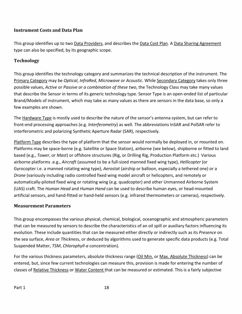
Instrument Costs and Data Plan This group identifies up to two Data Providers, and describes the Data Cost Plan. A Data Sharing Agreement type can also be specified, by its geographic scope.

Technology This group identifies the technology category and summarizes the technical description of the instrument. The Primary Category may be Optical, InfraRed, Microwave or Acoustic. While Secondary Category takes only three possible values, Active or Passive or a combination of these two, the Technology Class may take many values that describe the Sensor in terms of its generic technology type. Sensor Type is an open-ended list of particular Brand/Models of instrument, which may take as many values as there are sensors in the data base, so only a few examples are shown.

The Hardware Type is mostly used to describe the nature of the sensor’s antenna system, but can refer to front-end processing approaches (e.g. Interferometry) as well. The abbreviations InSAR and PolSAR refer to interferometric and polarizing Synthetic Aperture Radar (SAR), respectively.

Platform Type describes the type of platform that the sensor would normally be deployed in, or mounted on. Platforms may be space-borne (e.g. Satellite or Space Station), airborne (see below), shipborne or fitted to land based (e.g., Tower, or Mast) or offshore structures (Rig, or Drilling Rig, Production Platform etc.) Various airborne platforms .e.g., Aircraft (assumed to be a full-sized manned fixed wing type), Hellicopter (or Gyrocopter i.e. a manned rotating wing type), Aerostat (airship or balloon, especially a tethered one) or a Drone (variously including radio controlled fixed wing model aircraft or helicopters, and remotely or automatically-piloted fixed wing or rotating wing (e.g. quadcopter) and other Unmanned Airborne System (UAS) craft. The Human Head and Human Hand can be used to describe human eyes, or head-mounted artificial sensors, and hand-fitted or hand-held sensors (e.g. infrared thermometers or cameras), respectively.

Measurement Parameters This group encompasses the various physical, chemical, biological, oceanographic and atmospheric parameters that can be measured by sensors to describe the characteristics of an oil spill or auxiliary factors influencing its evolution. These include quantities that can be measured either directly or indirectly such as its Presence on the sea surface, Area or Thickness, or deduced by algorithms used to generate specific data products (e.g. Total Suspended Matter, TSM, Chlorophyll-a concentration).

For the various thickness parameters, absolute thickness range (Oil Min. or Max. Absolute Thickness) can be entered, but, since few current technologies can measure this, provision is made for entering the number of classes of Relative Thickness or Water Content that can be measured or estimated. This is a fairly subjective

Part 1 19

measure, however, since the qualitative nature of relative thickness or water content classes (e.g. sheen, emulsion), may vary among instruments and algorithms.

Auxiliary Oceanic and Atmospheric parameters (e.g. Wave Height, Wind Speed, Air temperature) may also be measured to determine the importance of processes such as mixing, weathering, or transport of a spill, while other chemical or bio-chemical air or water parameters may also be represented.

Oil Type Class can be specified, and to various levels of specificity. E.g., depending on the available information, oil type might be classed simply as Crude Oil, or more specifically as Heavy Crude. There is also provision for identifying oils that are specified by the ADIOS weathering model. Oil Condition may be specified broadly to be in a thin film (Sheen), a Continuous liquid form (typical of fresh oil floating on a calm surface), Emulsified or Dissolved (i.e., suspended, or dissolved in sea water, respectively). Other oil weathering products such as Mousse and Tar balls may also be specified.

Electro-Magnetic Spectrum Properties Excitation Wavelength or Frequency is used to specify the Transmitted signal in active sensors (e.g. the signal used to stimulate fluorescence or to set Laser color. It is not relevant for passive sensors. There is provision for describing up to three excitation signals. The Receiving Bands (Frequency or Wave bands) are specified in terms of conventional band names for microwave, IR, Visible and IR regions of the spectrum. Up to four bands can be specified (Primary, Secondary, Tertiary and Quaternary). Band Limits (Low End and High End) are used to specify the signals received by active and passive sensors. By convention in the Excel spreadsheet Instrument Table, frequency in GHz is given for microwave ( W)

instruments, while wavelength in microns is given for Optical and IR (Opt.) instruments. In the Spectrum Table and associated graphs, both limits and graphs are automatically given in both frequency and wavelength terms. The band Span is computed (automatically in the spreadsheet) as the difference between the band limits. The Number of Channels in each Band is also specified and the (mean) Spectral Resolution is computed as Band Span divided by that number (in appropriate units).

Part 1 20

Sensor Performance Criteria We now describe the sensor performance criteria that were developed for the project. These criteria were implemented and tested in the Excel spreadsheet system developed as part of the project. This spreadsheet-based sensor selection tool was developed to assist the project team, and subsequently future users, in identifying sensors and sensor suites suited for application to specific pre-defined historical, hypothetical or user-specified spill scenarios. It has also served as a ‘development platform’ for the browser-based sensor selection tool, developed during the second half of the project, which is intended to serve as a prototype for a web-based system that could be developed in a future project.

The criteria defined for the purpose of sensor evaluation are listed in Table 2, where they are placed in four convenient groups: Spill Sensing Capability, Data Accessibility, Hardware Accessibility and Instrument Costs and Data Plan. For each selection criterion, a set of five values may be assigned to it, and the corresponding performance scores, are specified. The order of presentation is similar to that adopted in the Excel spreadsheet system. Within this system, the criteria are applied to an expanding set of examples of particular sensor technologies. In the latest version of the spreadsheet database, a few criteria are assigned additional named values, but in all cases only 5 possible scores (1-5) are assigned (i.e. some name values are assigned the same score, meaning they have qualitative differences that do not significantly change instrument performance). A 5-point scale was chosen to allow for a central (or neutral) value and two extremes, with intermediate values in between. In addition, some studies suggest that a maximum of about five randomly placed objects can be enumerated visually by humans by ‘subtizing’ i.e. without counting! (Vetter, 2009). Against these criteria, the scores (on a scale of 1-5) assigned to each technology category or sensor may be used to compute a mean Performance Score. A more detailed description of the spreadsheet features and functions appears, including the computation of mean Performance appear in Part 4 and the Appendix of this report. That information is also collected into a separate Sensor Guide, which serves as a User manual for the Sensor Selection system.

Part 1 21

Table 2. Sensor Performance Criteria

Criterion Assigned Sensor Score and Corresponding Value

Spill Sensing Capability Group Score: 1 2 3 4 5

Operational Status Not Operating De-commissioned Commissioning Operating

Part time Operating

Continuously

Maturity Developmental Experimental Functional Prototype

Awaiting Launch

Operational

Detection Potential Improbable (< 20%) Unlikely (<40%) Even Chance

(40-60%) Likely (>60%) Near-Cert. (>80%)

Prob’y False Negatives

Improbable (< 20%) Unlikely (<40%) Even Chance

(40-60%) Likely (>60%) Near-Cert. (>80%)

Prob’y False Positives

Improbable (< 20%) Unlikely (<40%) Even Chance

(40-60%) Likely (>60%) Near-Cert. (>80%)

Data Accessibility Group

Data Access Type: Storage Media File Transfer Email Web Page Autodownload or User Display

Acquisition Lead Time Infinite Delayed

(< 7 day) Delayed (<3 day)

Delayed (<1 day)

Realtime (<3 hr)

Product Delivery Time Infinite Delayed

(< 7 day) Delayed (<3 day)

Delayed (<1 day)

Realtime (<3 hr)

Data Interpreter Capability Skilled Well Trained Basic Training Basic

Instruction Provided

Hardware Accessibility Group

Score: 1 2 3 4 5

Owner HQ Region Overseas Non Contig. Non US Contig. Non US Non-Contig. US Contig. US

Sensor Access Type Purchase Lease Rental Turnkey Full Service Availability (#

Units) 1 <= 2 <=5 <= 10 > 10 (99)

Deployment Planning Time > 5 (99) <= 5 <= 2 <= 1 0

Deployment Readiness > 5 (99) <= 5 <= 2 <= 1 0

Instr. Op. Capability Skilled Well Trained Basic Training Basic Instruction Provided

Autonomy Manual Operation

Manual Sampling Semi-Automatic Automatic Autonomous

Part 1 22

Instrument Costs and Data Plan Group Score: 1 2 3 4 5

Instrument Cost > $1,000,000 > $100,000 > $10,000 > $1,000 < $1,000 Installation Cost > $1,000,000 > $100,000 > $10,000 > $1,000 < $1,000 Initial or Fixed

Rental > $125,000 > $25,000 > $5,000 > $1,000 < $1,000

Regular Daily Rental > $125,000 > $25,000 > $5,000 > $1,000 < $1,000

A brief description and discussion of each of the performance criteria in each group shown in Table 2 is given below:

Spill Sensing Capability Maturity describes the Instrument Development Level of Maturity. It represents the level to which the technology or sensor has been developed, and is an indication of its readiness for oil spill operations. Developmental and Operational sensors are considered the least and most mature, respectively. In the Excel spreadsheet system such terms may be further qualified (in embedded comments), to aid the sensor analyst or user in deciding what value to assign for each criterion. For example, the values assigned to the Maturity criterion may be qualified as follows:

Operational Instrument Fully Tested and Operational

Awaiting Launch Instrument Fully Tested, Installed and Ready for Launch

Functional Prototype Sensor is a fully-functional and operational Prototype (First of a kind)

Experimental Some sensor functionality demonstrated experimentally

Developmental Sensor under design, construction or development, but not yet functional

Clearly, fully operational sensors are most likely to perform well in oil spill response situations, so these are allocated the highest score.

Detection Potential describes the probability (which ranges from 0%, or highly unlikely to 100%, or almost certain) that instrument will see a spill, if one is present. Since probability is difficult to estimate precisely; broader ranges are defined as Near-certain (>80%), Likely (>60%), Even Chance (40-60 %), Unlikely (< 40%) and Improbable (<20%). For brevity, only one limit of each range is defined. It is understood that if the probability were 10%, the Improbable range would be assigned, rather than the Unlikely range. i.e. the lower limit of the Unlikely range is 20%. In the Unlikely case, the instrument is quite unlikely to detect a spill if it is present, although it is definitely possible (probable). The other limits can be similarly qualified.

Part 1 23

Probability of False Negatives describes the probability of not detecting oil when it is present. The range of values that may be assigned is the same as that used for Detection Potential.

Probability of False Positives describes the probability of detecting oil when it is not present. The range of values that may be assigned is the same as that used for Detection Potential.

In practice, these probabilities are difficult to assign based on the available evidence, so in most cases values are assigned based on the expected performance of a relevant sensor class. There is more information on these probabilities for radars (where they depend on wind speed), than there is for other sensor technologies, so users should exercise caution in their interpretation.

Data Accessibility Data Access Type describes the type of data transfer that is normally used for the sensor, and who initiates data collection (operator, service or user). The faster, more highly automated and/or more convenient access types attract the highest performance scores.

Data Acquisition Time describes the time required to acquire the data from the sensor once the end user as requested acquisition. It maybe assigned a value in days, but will be automatically converted to a value range of Realtime (<=3 hrs), Delayed-time (<= 1 day, <= 3 day, or <=7 day), or Indefinite (>7 day). A Delayed-time of <=1 day could alternatively be described as near-real time. This time represents delays due to such factors as acquisition planning, sensor reprogramming, onboard processing and data downlink.

Product Delivery Time describes the time required to deliver the data to the end-user, once it has been acquired by the sensor. It may be assigned a value in days, but will be automatically converted to a value range of Realtime (<=3 hrs), Delayed-time (<= 1 day, <= 3 day, or <=7 day), or Indefinite (>7 day). A Delayed-time of <=1 day could alternatively be described as near-real time. This time represents delays due to such factors as ground-based processing, product generation and annotation and communication to the end user.

Note that a quantity termed the Data Latency could be defined to represent the sum of the Data Acquisition Time and Product Delivery time, in which case the ranges could be different. E.g. A Latency of less than 6 hrs might be considered nominal for real time acquisition and delivery, while one of 27 hrs could result from a near-real time acquisition combined with real time product delivery. Clearly, the shortest times attract the highest performance score.

Data Interpreter Capability describes the Interpreter Skill level required to generate the required product. If data interpretation is done prior to product delivery then these skills would be considered Provided. That case attracts the highest performance score. Otherwise a person with the necessary skill and time is needed which

Part 1 24

may incur additional expense or effort to generate the product, so the Performance score is reduced accordingly.

Hardware Accessibility Owner Headquarters (HQ) Region specifies the proximity of the Region to the US. The contiguous US states being considered the most accessible for oil spills affecting US OCS waters, attract the highest performance score, while non contiguous states or territories such as Alaska, Hawaii and Puerto Rico receive a slightly reduced score. Contig. Sensors owned by Contiguous Non US states would include those from Mexico and Canada. Non-contiguous, non-US states would by spanned by Central and South America and Overseas states are considered the least accessible, because costs and delays for approvals and transport to the US would likely be higher. A satellite sensor owned by a US company or agency will likely be more accessible than one owned by a Non-US or overseas one.

Sensor Access Type describes how the sensor may be accessed, and effectively measures the level of efficiency or convenience of such access (not costs per se, which are addressed separately below). Purchase attracts the low performance score because of the likely effort, delays and costs in securing funding, then purchasing and installing an instrument. On the other hand, a sensor that is configured to provide a full (paid or free) service, as is the case with some satellite sensors, attracts the highest performance score. Turnkey refers to a fully configured sensor that can be setup and run on demand, without making any new rental or lease arrangements. This could cover situations where the user already owns the instrument, or has an arrangement already in place to use the sensor when it is needed, and the instrument is fully functional and ready to be relocated if necessary and ‘switched on’.

Availability (# Units) describes the number of units of a particular sensor type that are potentially available for use. The number of units is scored by range with 1 unit receiving the lowest score and more than 10 receiving the highest score. The more units available, the better the chance, in general, of being able to obtain one to use in a particular oil spill operation. Availability will depend somewhat on the Maturity level of an instrument. If it is either of Experimental or Prototype maturity, there is likely to be, at most, one unit available, and even that might not be operational at the time it is required. Similarly most satellite sensors are unique. However, the use of constellations of similarly equipped satellites is increasing to provide redundancy in case of failure, or greater spatial or temporal coverage, while for certain airborne sensors, frequently more than 1 unit is available.

Deployment Planning Time describes the time required to arrange for use of the sensor, once the end user has requested that it be made available. It employs time scales similar to those adopted for the Data Acquisition and Product Delivery times but with different values (<= 1 day, <= 2 days, <=5 days), or Indefinite (>5 day. This time represents delays due to such factors as route planning, sensor platform transit, or orbital positioning, and forward deployment.

Part 1 25

Deployment Readiness describes the number of days normally needed to prepare the sensor and instrument platform for deployment from a forward base, once a request is formalized (e.g. at the time an order issued by a user is received by the operator). Alternatively, it could be considered the time required for the sensor to appear in the target area, once it is available at a forward base, or in the case of a satellite sensor, when it is on orbit, and ready for operation. The time ranges are the same as those for the Deployment Planning Time (see above).

Instrument Operator Capability describes the level of skill required to operate an instrument. The situation where an operator is implicitly provided attracts the highest score. This would be the case if the operator functions and costs are built into a service, such as ground operation of a government or commercially-owned satellite system, where the operator cost is subsumed within the product price. Operators may range from those needing only basic Instruction to those who are Skilled. By Basic Instruction, we mean only minimal training or instruction is required to operate the sensor. By ‘Skilled’ we mean that a high skill-level, or high level of training is required to operate the sensor. One might think that a skilled operator would be the most desirable case. However, an instrument is considered to perform better if an operator is already provided or if one with only minimal instruction is needed to operate it effectively, in which case the instrument attracts a high performance score. A skilled (high-performing) operator might be difficult to obtain within funding and time constraints for a deployment, so this case scores low for instrument performance.

Instrument Autonomy describes the degree of autonomy of sensor operation and sampling that the instrument exhibits. The values that may be assigned range from Manual, which implies manual operation is required to acquire data samples to Autonomous, which implies the sensor operates without operator intervention, once it is deployed. The Manual sensor, which scores low on instrument performance, might be operated with the aid of a computer or hardware user interface. But the implication is that the operator must be fully and actively engaged in the sampling operations performed by the sensor. The Autonomous sensor is able to function independently of an operator during deployment, although manual operations may be required during launch and recovery (e.g. for a subsea glider or some unmanned airborne vehicle, or UAV). Instruments such as gliders or UAVs that require a human pilot during routine operation would not qualify for Autonomous operation, but could be considered Automatic or Semi-automatic.

Instrument Costs and Data Plan

Several of the specifications were described under this group name. Here we discuss only criteria (i.e. those parameters that are scored) which fall within that group.

Instrument Cost refers to the cost of purchasing the instrument, and it is represented as a range of values from a value less than $1000 to one exceeding $1,000,000.

Part 1 26

Installation Cost refers to the cost of installing the instrument, including labor and materials to install it on its platform and to configure it for normal operational use. It is represented as a range of values identical to that used for the purchase cost i.e. from less than $1000 to exceeding $1,000,000.

Initial or Fixed Rental refers to the ‘up-front’ or ‘one-off’ cost of renting the instrument for a particular task or a specified term. It is represented as a range of values from a value less than $1000 to one exceeding $125,000.

Regular Daily Rental refers to recurring daily cost of renting the instrument, once the initial arrangement, and if necessary up-front costs have been covered, if necessary (see above).It is represented by the same range of values as is used for the Initial or Fixed Rental Cost (see above).

Part 2 27

Part 2: Specification of Scenarios

Employing Spill Scenarios The assessment of remote sensing systems to detect and analyze oil spills is greatly facilitated by defining a set of spill scenarios that span a wide range of possible configurations for a spill. These scenarios may be of three types. The first, and the easiest to define, is a scenario based entirely on the information available concerning an historical spill. If the spill was a large one, and even if it occurred before the advent of the internet, quite a lot of information can be gleaned about the spill characteristics and its impact. This is coupled with the known remote sensing response is a valuable resource for sensor assessment. The second is a hypothetical spill that is configured to fill gaps in the range of historical scenarios either in geographic space or the space of the various parameters that can be used to describe a scenario. Finally, there are actual spills which are currently of concern and require a prompt remote sensing response to define their evolving characteristics.

There are several reasons for defining such scenarios. They can be used to research the effectiveness of remote sensing systems and select those that are effective for particular purposes (as in this project). They can be used for planning purposes to help pose ‘what if?’ questions for training and modeling exercises. They could thus be used to support decisions on advance deployment of remote sensing instrumentation in anticipation of possible future spills in particular areas or seasons (e.g. Alaska during winter, when ice is present). They may represent the currently known characteristics (best estimates) of a currently evolving spill, to help guide remediation efforts and provide a basis for ongoing remote sensing mission plans (In this case a sensor selection tool could be integrated into the actual response process) . Finally, they can be used in debriefing exercises to help determine what worked and what did not, under particular spill conditions for the sensors that were deployed. In this study we primarily used the scenarios to evaluate the suitability for intended purpose of each remote sensing system. However, in an operational response they could be used to select/reject, or rank particular sensors for use under the prevailing spill conditions. One could also imagine sensor developers using them to decide for what kinds of spills a particular sensor design might be effective.

The factors considered in defining various oil spill scenarios are now described, and a range of spill scenarios spanning a variety of spill sizes and types is presented. In the Sensor Evaluation procedure followed in this project, these factors were combined with the Specifications and Performance criteria presented in Part 1 to produce an index representing the Suitability for Intended Use criterion, for a variety of Sensor systems. The Specifications and Performance criteria provide a measure of the relative performance of a sensor system against criteria that are independent of its class, as well as against criteria that could be considered integral to its class. The performance criteria thus allow a sensor system to be ranked in terms of its overall capabilities in oil spill detection and analysis, and as well as with respect to others in its class.

The development and application of Scenarios provided a way to assess the suitability of a particular sensor system for providing the most useful remote sensing data given the nature of the spill. Primary characteristics

Part 2 28

of a spill may be described by factors determining its timing and location, size and the type of spill, factors which might be considered to be either static (.e.g. time of the initial spill) or gradually evolving (e.g., the current oil discharge rate). An important secondary aspect, which can strongly affect the Suitability of Intended Use, is a consideration of the oceanographic and meteorological conditions prevailing, or predicted to prevail, at the time the next remote sensing survey is to be carried out. These factors are much more dynamic, and will ideally be defined when sensor deployments are planned. However, they can also be used for ‘What-If’ styles of analysis, or for sensor assessment under expected weather conditions based on the local climate. If the next survey is to be carried out at night, optical Lidar, microwave radar or thermal infrared (TIR) radiometer systems would likely produce useful data, but passive optical systems would not. However, if it is particularly cloudy TIR systems will also be of limited value. In clear, calm daytime conditions optical systems will likely be most useful, since microwave radar systems are particularly vulnerable to false positives when the sea is flat, and to false negatives when it is particularly rough. However, even optical systems are subject to ambiguities in sensing oil or natural organic slicks. If the local climate, such as in northern regions is characterized by frequent cloud cover, in addition to reduced daylight hours during winter, then forward deployment of microwave systems for the winter season is to be preferred over optical systems.

Scenario Definition Representative factors considered in defining various oil spill scenarios are illustrated in Chart B (see Part 1, Technical Approach, above). Referring first to the left side and center of the Chart: Once a spill scenario is identified, factors describing the spill’s location in time and space include the date and time of the event, the coordinates of the point of discharge, and the duration of the spill, indicating how long it has continued. The spill size is determined by such factors as the spill volume and discharge rate, coupled with the duration. The type of spill can be described in terms of Incident Type (e.g. blowout or ship collision) and Oil type and conditions (right and lower center of Chart B). The factors shown are representative of a more comprehensive list that has now been developed within the Excel spreadsheet and database system, described in the Appendix.

The range of spill scenarios defined is considered sufficient to span a broad range of locations, sizes and types, but is not unmanageably large. Where descriptions of actual spill scenarios occupying significant parts of the range are available, they are used. Where there are large gaps in the range, hypothetical spill scenarios have been devised to represent spills of the location, type and size that have not occurred, but could conceivably occur under circumstances that could warrant a response. The initial geographic focus was on the Gulf of Mexico, represented by data base entries for the Deep Water Horizon, Ixtoc and Texas ’Y’ spills. However, the range of spills considered from this, and other representative regions, has been gradually expanded, and now includes representative OCS spill off the US east and west coast, including Alaska.

A more complete list of the factors defining each scenario is provided in Table 3. For the Scenario Identification Group, examples of entries for the 1979 Ixtoc spill in the Gulf of Mexico are shown. For the other groups only

Part 2 29

column labels are shown. For numeric factors (e.g. Latitude), a unit of measurement is provided in the spreadsheet (not shown here), but no further qualification is needed. However, for alphanumeric factors (e.g. Spill Event Type, the choices provided in a drop-down list in the spreadsheet are provided in the table (in italics). For missing data a not available/not applicable flag (by convention represented by #N/A in Excel tables) is provided in the menu (not shown here).

Part 2 30

Table 3. Key Scenario Parameters

Parameter Parameter Values

Notes: Entries in Italic face represent actual string values of the relevant specification. Entries in normal face represent numerical value entries (except for web links and documents. Only single value examples are given in the first Group.

Scenario Identification Group

Scenario Name Short Name Geographic Region Country Location Event Date

Pemex Exploratory Well,Bay of Campeche Ixtoc Gulf of Mexico Mexico 3-Jun-1979

Scenario Analysis Group

Data Analyst (Initials) Event Name Event Date Event Time

Spill Location and Proximity to Land Group

Latitude Deg. Dec’l Min Hemisphere Longitude Deg. Dec’l Min Hemisphere Water Depth

Distance to Nearest Land

Distance to Nearest Island

Spill Type and Conditions Group

Spill Event Type: Well Blowout Well Leak Pipeline Riser Process. Facility Loading Facility Storage Facility Vessel Collision

Aggravating Condition: Explosion Fire Flood Hurricane Fatal Accident Power Failure Sinking Grounding Collision Flammable Gas Poisonous Gas

Initial Release Group Spill Source Type: Oil Platform Oil Well Oil Tanker Ship

Oil Barge Storage Tank Boat Release Date/Time Amount Released Inst. Spill Rate

Part 2 31

Estimated Spill Size Group Estimate Date/Time Spill Duration at

Estimate Time Spill Volume Spill Area Mean Thickness

Affected Coastline Length

Oil Type and Condition Group Oil Type Class: Any Oil Vegetable Oil Mineral Oil Mean Thickness

ADIOS Type Crude Oil Heavy Crude Medium Crude Light Crude Fuel Oil Heavy Fuel Oil Medium Fuel Oil Light Fuel Oil Gasoline Gas (LPG, LNG)

Specific Oil Type API Density Pour Point Temp Phase In-Water Geometry: Coherent Patchy Fingered Blurred

Diluted Layered Oil Condition: Continuous Emulsified Dispersed Dissolved

Mousse Tar Balls Oil Disposition: Onsurface Subsurface Bottom SubBottom

Sinking Rising Beached

Ocean Met Conditions and Water Properties Group Wind Speed Wind Direction Current Speed Current Direction Wave Height

Water Temperature Water Salinity Sediment Load

Key References Group

Reference Code(s) Reference Documents

Scenario Weblinks

An explanation of the meaning and rationale for certain key factors follows (details concerning other factors are provided in the Appendix). A brief description of each of the Scenario parameter groups and examples of the parameters and possible values is given below.

Scenario Identification Group This group provides the Scenario Name and describes its geography in terms of its location (Oil Spill Geographic Region and Location Name), the Water Body Type in which it occurs and the Oil Spill Country Location relative to the contiguous US states.

Part 2 32

Scenario Analysis Group This group identifies the analyst, as well as the Date and Time applicable to the analysis (e.g., the time of a planned remote sensing operation, or recent data update).

Spill Location and Proximity to Land Group The parameters in this group give the geographic location of the spill in which it occurs (its Latitude, Longitude and Depth and the Depth of Water). The Initial Distance to Nearest Land and to Nearest Island, provides an indication of its location relative to surrounding land. This gives an indication of the possible logistical or sampling constraints on remote sensing operations and possible impacts (e.g. a low resolution microwave radiometer might suffer land contamination near the coast, while a nearby island could warrant an assessment of possible oil impact).

Spill Type and Conditions Group This group describes the nature of the spill and its source, which qualifies the facility or circumstances accounting for the spill event.

Initial Release Group This group identifies the Spill Source Type, which is the type of structure actually discharging the oil. The characteristics of the initial release are provided by the Initial Release Date and Time of spill along with measures of spill size and rate (Amount Released and Instantaneous Spill Rate). In this group, the spill amount and rate of release are used to characterize a sudden or a continuous discharge, or a combination of these (for a nearly constant continuous discharge, the amount released could initially be zero). The Instantaneous Spill Rate factor can be revised in subsequent Analysis Events.

Estimated Spill Size Group This group provides subsequent estimates of spill size, and includes the date/time that these estimates characterized the spill (not necessarily the time the analyst made the estimates, which, likely occurred later).

Subsequent spill growth is tracked in this group by the factors, Spill Duration (computed automatically from the difference between the Estimate Date and Time and the Initial Release Date and Time) and the Estimated Spill Volume (given in both barrels and cubic meters), which could be derived from the Instantaneous Spill Rate, or assessed independently). The Estimated Spill Length and Width can be used to compute the Spill Area, assuming it is rectangular, and this combined with the Spill Volume estimate may be used to compute a Mean Thickness (though it is recognized that minimum and maximum thickness, or range are of greater interest). The length of Affected Coastline can also be specified if the oil has gone ashore.

Part 2 33

Oil Type and Condition Group The Oil Type Class and Oil Condition represent the same parameters and sets of values that are referenced in the Instrument Table (See previous chapter for discussion). There they represent the class and condition that can be detected by the sensor, while here they represent the prevailing spill characteristics. Specific Oil Type represents a number code that links to the OilTypeTable and associated type descriptors, while API Density, Pour Point Temperature and Phase (Gaseous, Liquid, Solid or Mixed) can also be specified. The In-Water Geometry describes the apparent (mainly horizontal) structure of the oil plume, while the Oil Disposition describes and its vertical location or distribution and relative motion through the water column.

Ocean Met Conditions and Water Properties Group This group collects together those parameters that provide supporting Oceanic, Atmospheric physical properties, as well as simple water quality indicators (salinity and sediment load). These can all be assigned numerical values if known. Both the direction and speed of the prevailing winds and ocean currents can be specified, while surface roughness is described by wave height and period. The intent is to capture those properties that could influence the detectability, trajectory or disposition of the plume and provide numerical values that could be used in modeling plume behavior. A more comprehensive range of Physical, Chemical and Biological Oceanic and Atmospheric Parameters are identified in the Specification Table (see Chapter 1 and Table 1). Those are used to specify which parameters may be detected and/or measured by the instrument under consideration, without regard to their potential ancillary value for diagnosing plume evolution.

Observer Constraints Group This group may be used to specify constraints on funding for sensors or sensor data and desired lead time for sensor data acquisition, as well as the levels of skill available for Instrument operation or data interpretation. The Instrument Operator and Data Interpreter Capability Skill and their corresponding values are the same as those used in the Instrument Table to describe the skill levels required for instrument operation or data interpretation. By matching the constraints with the requirements in the Sensor Scenario Matrix of the spreadsheet, potential shortfalls can be identified.

Application of Oil Spill Weathering and Trajectory Models The foregoing metadata, concerning spill size and type, as well as the more specific information on oil types and meteorological and oceanographic conditions, can be used to provide initial inputs into an oil spill model, such as the NOAA ADIOS oil spill weathering model, or the NOAA GNOME oil spill advection model (see below

Part 2 34

for details). Such models can be used to obtain estimates of spill size early in the development of the spill, before the slick begins to break up due to air/sea interaction processes. The models can thus provide estimates of likely spill size that would be useful for planning initial remote sensing operations. A detailed discussion of the application of such models, and oil spill modeling in general, is outside the scope of this report. However, a brief summary of the model capabilities and the types of information that can usefully be obtained from them about oil spill scenarios is given below:

NOAA ADIOS Weathering Model The Automated Data Inquiry for Oil Spills (ADIOS) model was first released by NOAA in 1994 to help oil spill responders forecast the weathering and other characteristics of oil spills. An updated and revised version ADIOS2 became available in 2000. It accounts for additional weathering processes including spreading, dispersion, sedimentation and emulsification, as well as spill cleanup options including dispersants, in situ burning and skimming. The model can be run on Mac or PC (Windows) personal computers and considering the complexity of the model, has a remarkably simple and convenient user interface. The model is based, in part, on somewhat idealized spreading and dispersal mechanisms first modeled by Fay (1971). Simulation based on these mechanisms might provide valid approximations of oil spreading upon release and its weathering and dispersal e.g. due to gravitational spreading, during the first few days of a spill. However, within about 5 days more complex ocean dispersal mechanisms, such as Stokes drift and Langmuir circulation (due to interaction of wind-waves and currents) are likely to dominate, so the model assumptions and approximations will break down. Preliminary tests performed using the model reveal that it can provide useful estimates of spill volume and area, and of the oil spill budget. The model is driven by specified oil type (obtainable from a comprehensive model data base), and prevailing weather conditions specified by the user. Thus it can be useful to provide scenario parameters that might not be available from in situ measurements, or previous remote sensing surveys.

NOAA GNOME Oil Spill Advection Model The General NOAA operational modeling environment (GNOME) model, is described as the modeling tool for the Office of Response and Restoration’s Emergency Response Division (see http://response.restoration.noaa.gov/oil-and-chemical-spills/oil-spills/response-tools/news-gnome-wizard.html). Like ADIOS2, it is available for download in PC (Windows) and Mac versions. GNOME can be run in a standard mode useful for educational and planning purposes. In this mode, it can be used to explore a variety of scenarios. It is supported by location files which provide ancillary geographic, meteorological and oceanographic data (or guidance on how to find these) for some specific geographic regions. It can also be run in a diagnostic mode that is used by oil spill response professionals for modeling particular spills. In this mode, additional spill trajectory and weathering information obtained from supporting models, as well as the results of current remote sensing surveys would normally be ingested into the model. A supporting tool, the GNOME Online Oceanographic Data Server, GOODS is an online tool that helps users access base maps and publically

Part 2 35

available ocean currents and winds from various models and data sources. GNOME can readily exchange files with Geographic information Systems (GIS) and according to the website, a new feature planned for GNOME is integration with ADIOS. Our tests reveal that GNOME can be used fairly easily to set up a spill scenario, based on available Location files. It can then be run to produce a ‘movie’ or successive ‘snapshots’ of the oil spill trajectory, as it evolves over a period of hours and days. Land boundary plots enable grounding of the spilled oil in coastal margins to be simulated. The model does not appear to offer a means to track spill volume or budget, nor does it allow remedial actions to be incorporated in the forecast (in contrast to ADIOS). However, an ancillary tool, GNOME Analyst ostensibly can be used to generate oil concentration contours, which could perhaps be used to estimate spill volume. However, that is evidently an ‘in-house’ tool that appears not to be publicly available. There is also a capability to utilize the results of airborne visual or remote sensing surveys to define the status of the spill to initialize a new forecast (see NOAA, 2002 and NASA, 2004 for details).

According to the NOAA GNOME website FAQ, differences between AIOS2 and GNOME include the following: “GNOME uses a simplistic 3-phase evaporation algorithm, which is appropriate for simple drills and educative comparisons. The oil weathering model, ADIOS2 (Automated Data Inquiry for Oil Spills), has the better evaporation and oil fate estimates compared to GNOME. ADIOS also has an extensive oil library.” There are several other oil spill models that could potentially be used to help specify scenarios for use with the remote sensing technology selection spreadsheet developed within this project. One such model OilMap, available commercially, includes a variety of features and modules for addressing several types of spill (http://asascience.com/software/oilmap/). A useful review of oil spill trajectory modeling in the presence of ice, and of associated dispersal mechanisms, is provided by Drozdowski et al. (2011). The available models, their capabilities and potential for further enhancement for this purpose warrants further testing and evaluation, and such activity could be proposed as a useful follow on to the current project.

Model-based Scenario Development A combination of ADIOS2 and GNOME simulation runs was conducted for a relatively small (1000 bbl) hypothetical oil spill in eastern Long Island Sound. The model input parameters, which include spill size and date, oil type and prevailing weather conditions, among other factors were defined in a consistent manner for both models. This enabled their complementary output features to be exploited to provide a comprehensive assessment of the spill. The example chosen was that described in the GNOME user guide, which includes use of the Central Long Island Sound Location File.

Spill predictions were run for 1 to several days (the models impose differing limits on the forecast duration). Estimates of spill trajectory, area and length of coastline affected were made using GNOME, while ADIOS 2 was used to provide estimates of oil spill volume and budget, taking evaporation into account. Differences between the data requirements and capabilities of the two models were noted. For example, ADIOS allows actual crude oil of specified density and other characteristics to be specified (we chose Bay Marchand, LA medium crude oil with an API density index of 26.1), while GNOME allows only gross oil types to be specified

Part 2 36

(we chose Medium oil, which as a density range of 22.3 < API < 31.1). ADIOS2 can generate oil spill volume and track changes due to weathering. However, GNOME only provides a visual impression (map-based movie) of the spill trajectory, with only a relative density indication (in the form of scattered ‘splots’). GNOME Analyst can evidently provide oil concentration contours, but this was not available. A very useful feature of GNOME is the provision of a ‘Minimum Regret’ solution, which represents the uncertainty associated with the primary ‘Best Estimate’ solution. In an oil grounding situation, this allows the likely and ‘worst case’ linear coastline impact to be assessed.

For our hypothetical Central Long Island Sound oil spill scenario, the combined output of the models provided the following spill estimates after a 24 hour prediction period: Of the original 1000 bbl spill, the estimated spill volume remaining after evaporation of about 150 bbl and dispersal of 25 bbl, was approximately was 825 bbl. The maximum spill area (on water) was 43 kilometers squared. The best guess length of affected coastline was 5.6 km, with a minimum regret value (representing the uncertainty range) spanning 13.9 km, or twice as long. The grounding occurred along the central northern coast in response to a prevailing 15 knot southerly wind. Experiments performed with a weak 5 knot easterly wind resulted in the oil being swept westward into the inner sound. Using GNOME, the oil spill oscillated E-W with the tide, while it drifted westward, but it had not grounded after 72 hr, so a longer simulation time would be needed to explore its impact on the coast. ADIOS2 can be used for forecast periods up to 3 days (72 hr), but it only provides measures of the oil budget changes and not trajectory or coastal impact predictions. While the two models can be used in a complementary fashion as described here, a more comprehensive model that incorporates trajectory, weathering and spill budget information in one system would be easier to apply for our purpose of developing hypothetical spill scenarios for assessing remote sensing technologies.

Part 3 37

Part 3: Sensor Selection and Evaluation

The Sensor Survey A comprehensive survey and classification of single-band sensors, multi-band sensor packages and sensor suites has been conducted. The results are being made available to potential users in the form of a searchable data base, spreadsheets and tables, and a visual representation of the sensors and their alignment with respect to the electromagnetic (E-M) spectrum. For each practical sensor system, we determined the operational, prototype or developmental status, and current availability and, when available commercially, the cost. Platform/mounting and operational requirements are also described when available, and levels of automation and requirements for human intervention in instrument operation and data processing and interpretation are considered.

The IDAOS Excel Workbook The Instruments to Detect and Analyze Oil Spills (IDAOS) Microsoft Excel workbook, developed for this study, effectively identifies selected technologies that meet the evaluation criteria, under the circumstances of one or more historical, hypothetical, or optionally user-specified, oil spill scenarios. In this third part of the technical report, and in the Appendix, we describe the intended purpose, features and structure of the IDAOS spreadsheets software and data files, and explain the content, search methods and interpretations of the data contained in it.

The Excel workbook (which in Excel terminology represents a single file with a collection of closely related spreadsheets comprising what we term here, a spreadsheet system. The IDAOS workbook or spreadsheet system was developed to provide a data repository of, and a systematic tool for organizing, descriptive textual and numerical information on the oil spill sensing systems and scenarios investigated in this study. It was developed initially to aid the NRL study team members in conducting, and also saving and viewing, the results of the sensor survey during the course of this study. However, it is also intended to facilitate the assessment of sensors of various classes, not only during the study, but after its completion, both to allow comparisons to be made among sensors of each class and subclass, and to facilitate evaluations of the capability of the sensors for application to specific oil spill scenarios. The latest and final project version provides an effective snapshot of the current characteristics and capabilities of selected sensors. However, it is also intended to be readily updateable, with provision for the addition of new sensors and scenarios, as instrumentation evolves and as new oil spill scenarios become available for scrutiny. The reader is referred to the Appendix for a description of the structure and use of the Spreadsheet software. The following sections describe the rationale and main features of its design. First we discuss certain caveats. We then describe built-in sensor performance and suitability scoring procedures.

Part 3 38

Caveats Regarding Spreadsheet Function and Use The IDAOS spreadsheet is designed to contain, organize and give ready access to, a comprehensive data set of remote sensing systems for oil spill detection and analysis, and a wide selection of historical and hypothetical oil spill scenarios, with a capability for entering user-specified ones. It is also intended to provide a simple scoring system to quickly provide a convenient summary, and also more detailed evaluations, of the potential performance and suitability of a sensor for application to the scenario under consideration. In essence, the scoring system assigns a performance score 1.00-5.00 (5.00 being best) that represents the sensor’s overall performance for oil spill applications, and a suitability index, also on a numerical scale of 1.00-5.00, but conveniently simplified to an assigned letter ‘grade’ A-E (A being most suitable) that represents its suitability for application to the circumstances and conditions of a particular oil spill. Since the performance score and suitability index are largely, but not completely, independent there is a wide range of possible combinations of the two evaluation measures. For example, an instrument might perform well in general, but be unsuited to the conditions of a particular spill, or may be well suited, based on its type, but not be the best performing sensor in its class. The user should appreciate that while the resulting evaluation procedure is itself objective (based on logical decision rules), considerable subjective expert (and in some cases non-expert!) judgement was required to decide what values to assign to particular sensors and criteria, and how these might be ranked or scored to determine instrument performance.

Accordingly, the spreadsheet should be considered as an aid to decision making. It is not intended to usurp the oil spill professional’s role, rights and obligations in evaluating the available sensors and deciding which ones to deploy to detect oil spilled under particular circumstances and conditions. Rather, it is intended to support this role. The quality of the evaluations will depend in part on the conceptual structure of the decision rules. At its best, the tool can only be as good as the data and decision rules contained in it. While every effort has been made to use the available published and online literature describing sensor capabilities, applications and historical spill parameters, coupled with team member experience, the data are necessarily incomplete and variable in quality, and thus less than perfect for its intended use.

The authors consider that the spreadsheet is the best that could be constructed with the available resources, and believe it should provide a valuable foundation for future development and refinement of the Sensor selection spreadsheet system. More generally, it should supplement the oil spill response community’s current capabilities to select and deploy the most effective remote sensing resources to detect and analyze future oil spills.

Part 3 39

Instrument Performance Among the parameters used to describe sensors in the IDAOS Instrument worksheet, a subset has been selected for use in determining the expected relative performance of instruments for use in detecting and monitoring oil spills. These are assigned a raw integer score from 1 (worst) to 5 (best), representing how well the sensors are expected to perform against specific criteria. A decimal mean score (range 1.00-5.00) that represents the sum of the individual raw criteria scores divided by the number of criteria, for each sensor, can be used to rank them within particular classes or subclasses, and determine which ones might best meet general requirements for detecting or monitoring oil spills. This mean performance score is intended to help the user answer such questions as “Which is the best Synthetic Aperture Radar (SAR) sensor to use for an oil spill survey?”, where ‘best’ applies to that instrument which collectively meets the criteria to the greatest extent (i.e. with the highest total performance score). Instrument parameters that are not contained in the performance criteria subset are assumed to be descriptors (or specifications) that while potentially useful in choosing, configuring or operating the instrument under particular circumstances, do not currently represent any particular relative performance advantage. They are provided for the convenience of the user, even though they might not be decisive in the sensor selection process.

Suitability for Intended Use The development of two sets of parameters in separate worksheets, one that describes the instrument characteristics (including the specifications subset mentioned above), and a largely independent one that describes the scenarios, allows us to construct (in a separate worksheet) a cross-reference matrix (the ‘Sensor-Scenario Matrix’), that allows the relationship between the two sets to be specified. The conceptual structure of this Sensor-Scenario Matrix is illustrated in Chart E. At the intersection of each instrument parameter (matrix column) and scenario parameter (matrix row), a decision rule can be (and in more meaningful cases is) defined. These rules allow the relationship to be assigned a raw index value (in the range 1-5 or symbolically, E-A), that represents the suitability of the sensor for application to the scenario, with respect to that particular combination of parameter values; with a suitability of 1 (or E) being least suitable and 5 (or A) being most suitable.

Part 3 40

Chart E.

Chart E illustrates the conceptual structure of the Sensor/Scenario matrix which incorporates decision rules that relate selected pairs of Scenario parameters to Sensor Performance parameters. Together these factors contribute to a suitability index that combines the results of applying corresponding decision rules.

The ensemble of indices (represented by the sum of individual index raw values, divided by the number of decision rules applied), or the ‘suitability index’, also on a decimal scale of 1.00 – 5.00 (or E-A), provides an assessment of the overall suitability of use of the instrument under consideration, for application to the scenario of interest. This suitability index is intended to help the user answer such questions as “Which type of instrument best meets the requirements for detecting oil, given the characteristics, and under the prevailing conditions, of a particular spill?”, where ‘best’ applies to that instrument which is found to be most suited to that intended purpose. The Sensor-Scenario matrix is relatively sparse. That means only a few of all possible pair-wise combinations of Sensor and Scenario parameters have meaningful relationships and are currently

Part 3 41

related by a decision rule. This will change as experience with Sensors and Scenarios allows additional meaningful new decision rules to be formulated. Thus, the filled cells of the Sensor Scenario Matrix represent our current understanding of how sensor performance dictates suitability for intended use, with respect to a particular Scenario, while the unfilled cells indicate where is no currently known relationship between the relevant Instrument performance parameter and scenario parameter pair. A more detailed discussion of the sensor scoring and evaluation system is provided in the Appendix. Part IV of this report provides an evaluation of the selected sensors that follows these principles, and is based on the various sensor and scenario parameters, and on the approach to scoring sensor performance and suitability for intended use described above.

Part 4 42

Part 4: Preferred Sensors

Sensor Selection A comprehensive survey and classification of single-band sensors, multi-band sensor packages and sensor suites, and their performance within each technology class has been conducted. The resulting metadata, including instrument specifications, performance criteria, and scores are contained in the IDAOS spreadsheet and associated reference files. Based on these metadata, sensors can be sorted and ranked in various ways to reveal the potential performance of each sensor, within its class. Historical and hypothetical spill scenarios, user-defined scenario entry, and the Sensor/Scenario matrix allow the range of sensors available for use during particular types and sizes of spill, and the types of sensor platform and deployment mode to be evaluated. This allows the general characteristics of those classes of sensor that are best suited to these spills to be identified. In this chapter, descriptions of spill type, platform or mission type (or sensor deployment mode), and sensor class, as defined in the IDAOS spreadsheet, are employed as a basis for identifying preferred sensor types considered best suited to particular applications and conditions.

For each preferred sensor system, we use the specifications and criteria encapsulated in the spreadsheet to describe the capabilities that make it one of the better performers in its class, or one that is best suited for application to the type of spill and prevailing conditions. It should be emphasized that there is no right or wrong choice of sensor. The particular sensor selected by a remote sensing professional, or spill response specialist under given conditions, and with the available resources or imposed constraints might differ from the one we choose, based on the Sensor Selection evaluation, to be the preferred sensor, either for technical or logistical reasons.

The performance scores are based on criteria related to the design, availability and operation of the sensor. They are used to assess sensor performance in the context of oil spill detection and analysis, but do not depend on the specific characteristics of a spill, and they are not intended to indicate performance for other applications. In contrast to the Performance score, the Suitability Index assigned to a sensor depends strongly on characteristics of the particular spill scenario, such as spill size, time, and location, and it can change significantly from spill to spill. The evaluation given below, which is based largely on application of the IDAOS Sensor/Scenario matrix, should provide a useful starting point and guide as to the most appropriate selection given the characteristics of historical spills and the scenario at hand, as described by user-specified information entered into the IDAOS scenario data base. However, professional judgement and experience, and the particular circumstances of a particular spill might warrant selection of a different sensor type or even a different class of sensor. In that case, the sensor data base and the associated filtering and sorting capabilities of IDAOS can be used to consider the strengths and weaknesses of alternative selections.

Part 4 43

Sensor Performance by Category and Class The performance of sensors based on criteria specified in IDAOS, and the scenarios described therein, can be readily obtained by applying EXCEL’s built-in sort features to the IDAOS Instrument Table. The results of two such sorting operations are presented in Tables 4 and 5. Others may be created based on the variety of sensor characteristics contained in the Table, but this one gives a useful overall summary of the State-of-the-Art that arises from the instrument survey performed for this project. Table 4 shows the top three sensors in each class based on the Primary and Secondary Categories defined in the Instrument Table. Note that the Performance Scores are based on the Criteria and associated scores appearing in the IDAOS Criteria Table. It does not take into account other sensor characteristics contained in the corresponding Specification Table. Those specifications might be needed to deploy and work effectively with, or understand the technical capabilities of, a particular sensor, but are considered to be neutral with respect to their effect on performance.

Part 4 44

Table 4. Sensor Performance By Category Primary Category Secondary Category

Optical-UV, Vis, Nir Active

Sensor Short Name Sensor Technology Class IDAOS SensorNumber

Performance Score

MEDUSA-LFS Radiometer 9 3.65 CALIOP Lidar 36 3.40 CATS Lidar 37 3.40

Optical-UV, Vis, Nir Passive

HumEye Eye 45 4.55 TRACS AS Vis Digital Camera 42 4.15 MODIS Multispectral Radiometer 6 4.05

InfraRed-SW, MW, LW Passive

TRACS AC IR Digital Camera 44 4.40 IRLS Multispectral Radiometer 40 4.20 TIRS Multispectral Radiometer 13 4.15

Microwave Active

Radarsat-2 SAR 17 4.30 CSK SAR 18 4.30 TerraSAR-X SAR 19 4.25

Microwave Passive SMOS Radiometer 3 3.75 OPTIMARE-MWR Radiometer 10 3.65 STARRS Radiometer 2 3.30

Part 4 45

Table 5 shows the result of sorting on Sensor Primary Category and Technology Class. The corresponding sensor platform type is also shown. Only the best performing sensor in each class is shown in this case. The two Lidars are included because their scores were tied, while the two Multispectral Radiometers fall into different Primary Categories, so both are listed.

Table 5. Sensor Performance By Technology Class

Sensor Technology Class Sensor Short Name (ID #) Primary Category Platform

Type Performance

Score Digital Camera TRACS AS IR InfraRed-SW,MW,LW Aerostat 4.40 Eye HumEye (45) Optical-UV,Vis,Nir Helicopter 4.55 Fluorosensor MEDUSA-LFS (9) Optical-UV,Vis,Nir Aircraft 3.65 Hyperspectral Radiometer Hyperion (15) Optical-UV,Vis,Nir Satellite 4.00 Imaging Spectrometer WV-1 (29) Optical-UV,Vis,Nir Satellite 4.05 Lidar CALIOP (36) or Optical-UV,Vis,Nir Satellite 3.40 Lidar CATS (37) Optical-UV,Vis,Nir Space Station 3.40 Marine Radar MIRAS OSD (23) Microwave Ship or Rig 3.70 Multispectral Radiometer IRLS (40) InfraRed-SW,MW,LW Aircraft 4.20 Multispectral Radiometer MSI (20) Optical-UV,Vis,Nir Satellite 4.20 Radiometer SMOS (3) Microwave Satellite 3.75 SAR Radarsat2 (17) Microwave Satellite 4.30

SLAR MEDUSA-SLAR (7) Microwave Aircraft 3.30

Spill Types and Representative Examples The various types of spills can be conveniently classified under several broad categories by combining various combinations of values of the Spreadsheet spill scenario parameters (Spill Event Type and Spill Source Type, Table 6). They may be further qualified with references to the size (Table 7) and duration (Table 8) of the spill, and the type of water body in which it occurs (Table 9). Size may be specified by the volume of oil spilled or by the linear dimension of the plume. The duration may be specified by the time in which oil is actually being discharged, or by the time required to complete oil recovery operations. In the Categories shown in the table, any combination of Spill Source and Spill Event Type is allowed. Simple number codes (to facilitate possible future numerical coding procedures) are also assigned to the various Category values in each table, and in the case of spill volume (in bbl), this is an indication of the logarithmic (base 10) magnitude of the spill.

Part 4 46

Table 6 Spill Type Categories

Table 6 assigns five broad Categories (Column 3) which collectively represent the Spill Source Types and Spill Event Types listed, independently of one another, in Columns 1 and 2, respectively. Representative examples of spills falling into this category are also shown (Col 4).

Spill Source Type Spill Event Type Category Name(No.)

Representative Examples

Oil Tanker Ship Spill Vessel Spill (1) Exxon Valdez, Kirby Oil Tanker Ship Vessel Collision Mega Borg Oil Tank Barge Vessel Allision Cargo Ship Vessel Grounding Boat Discharge Dumping Lightering Oil Platform Well Blowout Platform Spill (2) DWH, Ixtoc Oil Well Well Leak Riser Pipeline Leaking Pipeline Pipeline Spill (3) Refugio Broken Pipeline Storage Tank Process Facility Storage Spill (4) Loading Facility Storage Facility Drainage Outlet Leaking Pipeline Drainage Spill (5) Refugio

Broken Pipeline

Table 7 Spill Size Categories

Table 7 assigns eight broad Categories of spill size (Column 2) based on spill volume (bbl). A simple number code 1-8 is assigned to these categories based on the logarithmic (base 10) magnitude of the spill. The category names provide a convenient short hand for describing spill volume range.

Estimated Spill Size [bbl]

Size Category Name(No.) Representative Examples

< 10 (10^1) Micro (1) Oil Rig 2 (Hypothetical) < 100 (10^2) Very Small (2) < 1,000 (10^3) Small (3) Long Island (Hypothetical) < 10,000 (10^4) Moderate (4) Selendang Ayu < 100,000 (10^5) Medium (5) Santa Barbara < 1,000,000 (10^6) Large (6) Exxon Valdez < 10,000,000 (10^7) Very Large (7) DWH-Final < 100,000,000 (10^8) Mega (8)

Part 4 47

Table 8 Spill Duration Categories

Table 8 assigns six broad Categories of spill duration (Column 2) based on the time range during which significant spill volumes were reported (Column 1). A simple number code 1-6 is assigned to these categories. The category names provide a convenient short hand for describing spill duration. Representative examples are also shown (Column 3).

Time Range Duration Category Name(No.) Representative Examples

< 1 day Transient (1) 2 – 7 days (spans 1 week) Short-term (2) Oil Rig 2 (Hypothetical) 1 – 4 weeks (spans a month) Medium-term (3) Refugio 1 – 12 months (spans a year) Long-term (4) DWH 1 – 3 years (spans a triennium) Persistent (5) Exxon Valdez > 3 years (indefinite) Chronic (6) Taylor spill

Table 9 Spill Water Body Categories

Table 9 assigns seven broad Categories of water body (Column 2) based on more specific water body types (Column 1). A simple number code 1-7 is assigned to these categories. The category names provide a convenient short hand for describing spill duration. Representative examples are also shown (Column 3).

Water Body Type Water Body Category (No.) Representative Examples

Open Ocean Open Sea (1) Argo Merchant Open Sea DWH, Mega Borg Shelf Sea Semi-enclosed Sea (2) Santa Barbara Semi-closed Sea Intracoastal Waterway Sound Exxon Valdez Sea Coast Coast (3) Refugio Littoral Zone Selendang Ayu Barrier Lagoon Lagoon (4) Reef Lagoon Fjord Estuary (5) Estuary River Ship Channel Channel (6) Kirby Barge Port Canal Eagle Otome

Part 4 48

Coastal Lake Lake (7) Inland Lake

Sensor Deployment Modes Considering the variety of spill sizes and types spanned by the generalized spill descriptions provided in the previous sub-section, it is possible to identify a variety of sensor deployment modes. These are characterized by certain spill sensing applications, geographical contexts and sensor platform types that are relevant to the requirements of particular spill-related activities. The main types of application, geographic context and sensor platform that we have identified are first described, then commonly used and representative examples of deployment modes (characterized by the combination of those three factors) are analyzed. This leads to the identification of preferred sensor types best suited to use in the various deployment modes. In some cases, at least, these deployment modes could be viewed as particular mission types. Accordingly, in subsequent text we occasionally use the term ‘mission type’ as a short hand for ‘sensor deployment mode’. However, the specification of different standardized mission types is a current topic of discussion among oil spill and remote sensing professionals, so at this time we consider that term to be somewhat vague, and dependent upon the context.

Sensor Application Types Common Sensor Applications that we have specified (Table 10) may be broadly divided into Proactive (Pre-spill) or Reactive (Post-spill) time frames, with either short-term (< 1 month), medium-term (< 12 months) or long-term duration (1 or more years), and they may be of a Tactical (e.g. remediation) or Strategic (e.g. damage assessment) nature. As a general rule, the geographic context will be determined by the water body or, more specifically, by the geographic region being protected (e.g. by monitoring in case a spill occurs), or those in which a spill has just occurred.

Part 4 49

Table 10 Sensor Application Types

Table 10 identifies three broad Categories of spill application (Column 2) based on the time range during which significant spill volumes were reported (Column 1). A simple number code 1-3 is assigned to these categories. The category names provide a convenient short hand for describing the spill application. A description of the applications is given in Column 3.

Application Type Application Category (No.) Description

Contingency Planning Proactive (1) Education, conduct ‘What If?’ and ‘Worst Case’ desk studies and response training exercises

Strategic Baseline Studies Proactive (1) One-off or occasional studies of areas considered vulnerable to spills and their impact.

Monitoring Proactive/Reactive (3) Routine Sampling, Change Detection, Oil Detection and Alerts, and/or Enhanced Sampling

Impact Assessment Proactive/Reactive (3) Assessing predicted (tactical baseline) and/or actual spill impact areas.

Regulation and Litigation Proactive/Reactive (3) Gathering time sensitive data and ensuring archival along with complete time and location data.

Tactical Response Reactive (2) Determining the spill’s current location and size, and it’s evolution in time and space

Tracking and Mapping Reactive (2) Providing guidance for planning subsequent Remediation and Impact Assessment activities.

Tracking and Mapping Reactive (2) Providing data for input to or validation of oil spill trajectory and weathering models.

Strategic Damage Assessment Reactive(2) Extensive and/or recurrent sampling to

assess environmental/ecological damage

Recovery Studies Reactive(2)

Extensive and/or recurrent sampling to assess environmental/ecological recovery over time, with or without prior remediation.

Applications such as identification of high-value areas requiring regulatory protection, and identification of structures vulnerable to failure are very large and important applications that may use remote sensing methods for infrastructure monitoring and maintenance. However, these topics are considered outside the scope of the present work and have not been included among the listed applications.

Part 4 50

Sensor Platform Types Sensor platforms (not to be confused with Oil Production Platforms or ‘Drilling Rigs’, but recognizing that those could be used as sensor platforms as well) comprise supporting structures or vehicles for carrying the sensors and supplying them with resources such as power, lighting and communications facilities or infrastructure that are necessary for their operation and deployment in an area of interest, and for collection and distribution of the resulting data. Examples of various types of Sensor platform are illustrated in Chart D. With respect to the water body, the sensor may be deployed beneath, on, or above the surface, installed in a temporary or permanent configuration, and may be fixed in location, or mobile during operation. In addition, it can be internally recording and/or networked (via hardline or WiFi) for routine real-time or near-real time data communication etc. We further note that only a small number of the sensors, or more particularly, sensor suites that we surveyed, other than satellite sensors, have at least near real-time capability.

Chart F.

Part 4 51

Chart F illustrates some of the different categories of sensor platform and provides examples of particular platforms that may be in use.

Before proceeding, we should distinguish between in situ and remote sensing systems. By in situ sensors, we mean systems that make observations, and possibly take samples (for immediate or later analysis), within the immediate environment of the sensor, and specifically at the location of the sensor detection hardware or probe. This represents an important and large body of technologies for environmental measurements and increasingly, for oil spill detection and analysis, which however, is outside the scope of this work. It is not discussed further in the associated reports. By remote sensors, we mean systems that make observations at locations that are well removed in space from the immediate surroundings of the sensor and its platforms.

Most of the above-mentioned characteristics of remote sensing systems are described by parameters and corresponding value entries in the IDAOS spreadsheet. In all cases, the sensor platform is assumed to meet the operational requirements of the instruments. Given this assumption, we can divide the sensor platforms by the relationship to the water (or land) surface, and broadly group sensor platforms as follows:

Undersea Vehicles and Platforms (Beneath Surface)

These include fixed moorings, bottom mounted tripods, Autonomous Undersea Vehicles (Gliders) and Remotely Operated Vehicles (ROVs) and bottom mounted platforms equipped with water column profilers. There is an extensive range of in situ sensors used for oceanographic studies, but only a few such systems support remote sensing capabilities, and fewer still are designed for oil spill applications. We can only touch on the case of sub-surface systems, since they are still largely experimental or at best, developmental, with respect to oil detection and analysis. Examples include Induced Potential (Wynn and Fleming, 2012), in-water LIDAR/fluorescence, typically deployed from ships, and Glider-mounted Optical and Sonar Instruments (e.g. various kinds of multi-beam bathymetric scanners and side-look sonar).

As far as we are aware, there are no Commercial Off-the-Shelf (COTS) remote sensing (as distinct from in situ) systems specifically adapted to oil spill detection and analysis applications that operate from sub-surface platforms. A possible exception is subsurface gliders, for which an oil spill monitoring application has been demonstrated. There are no such platforms in the data base. They could be included if additional specifications and criteria that are characteristic of sub-surface instruments were added to the spreadsheet system. However, there are potential problems with probe contamination, in case they encounter concentrations of oil that significantly exceed background levels, and such issues would need to be resolved satisfactorily before operational use of COTS systems is considered feasible.

Surface Platforms (On Surface)

These include various types of moored and drifting buoys and floats, and autonomous gliders propelled by Waves or Sails, which can carry on board sensors and depth profilers capable of sampling at various depths or locations trailing beneath and/or behind the glider.

Part 4 52

Coastal, Island or Offshore Oil Platforms (Above surface)

Platforms in this group are usually mounted on structures fixed to towers, buildings or other supports erected on prominent land features (e.g. a headland), harbor buildings, jetties or offshore oil rigs. Examples may include Coastal Radars (e.g. CODAR) and Marine Radars or ship radars. Their use in a configuration designed for oil detection and analysis has been demonstrated, and at least in the case of Marine Radars, there are several COTS systems available, and these are described in the IDAOS database.

Part 4 53

Ships, Aircraft (including UAVs or drones), Kites and Balloons

This large group of platforms, which includes the very commonly used ships and aircraft, along with more recent experimental platforms consisting of kites and a few kinds of free-drifting or tethered balloons (aerostats) and drones, may be used in a variety of applications ranging from routine surveillance through large-scale strategic surveys to tactical response (remediation). This type of sensor platform has the combined advantage of both horizontal (positioning) vertical (altitude) mobility, which provides a range of options for varying the geographic coverage, timing and resolution of the associated remote sensing instruments.

Satellites

While Aircraft platforms provide a high degree of flexibility in deployment, location and timing (once they are dedicated to a mission), there is considerable advance planning and cost associated with both routine and spill contingent deployments. They are also subject to a strong (and in the case of Unmanned Airborne Systems, UAS, rapidly evolving) regulatory environment. This can make them difficult to deploy routinely, over large areas, or at short notice, in response to a particular oil spill event.

Though subject to higher initial cost to launch and maintain in operational mode, satellites can often provide data on a routine basis, at relatively low cost to the user. This is because the labor associated with the platform development, launch and operation, and associated sensor data acquisition, and sometimes the final product processing and interpretation is often centralized, and may be subsumed within the operational costs. Depending on whether the satellite is government or commercially owned (or a combination of both), these costs may be passed on to the users, but usually only in proportion to the amount of data they acquire. In some cases, such as government-owned satellites, data are provided to the user at no cost (eg., NASA Modis data). Satellites are also subject to orbital constraints (e.g. repeat or revisit periods) which dictate when passes may occur over particular locations. However, there is a wide range of satellites and sensors available, that exhibit a variety of orbital and sampling characteristics. These allow sensor data to be selected to best meet the requirements of particular spill scenarios, within the spatial and temporal constraints of the satellite and sensor specifications. Some satellite systems provide for customized targeting of particular geographic areas, but this usually requires prior arrangement and can increase costs.

Deployment Mode Descriptions The main deployment modes, or mission types, that we consider useful in evaluating and identifying preferred sensors can be described succinctly by identifying three relevant factors, namely, the application, geographic context and possible sensor platform types. The mission types considered by no means form a comprehensive set, but are considered representative of a significant number of possible sensor deployment modes. Modes that are frequently considered are now discussed. However, additional combinations of these three factors might be employed in exceptional circumstances.

Part 4 54

Monitoring of Spills from Oil Platforms on the Continental Shelf

Using the above definitions, this deployment mode covers applications that involve the monitoring of a semi-enclosed (shelf) sea using remote sensing instruments located above surface in the air or space above an oil platform or on nearby Coastal, Island or Offshore Platforms. Typical deployments would involve routine sampling over the medium to long term (multi-year deployments), though shorter deployments could be used in the case of a temporary platform (e.g. for a drill test site). The assumed mission goal is to provide early detection of oil spills emanating from sources on, or close to, an active (manned) test or production oil platform. Depending upon the drilling and oil transfer methods used, possible spills could involve sources such as the Oil Platform itself, the Oil Well or an associated Oil Tanker or Pipeline (used for transferring oil to shore). A large spill, especially one resulting from an incident that significantly changes the operating conditions on the rig, will almost certainly be noticed and reported very soon after it occurs, thus triggering an emergency response. It is the smaller and less obvious spills due perhaps to accidental or chronic discharges or other mishaps that do not obviously disturb normal rig operations, which need to be detected automatically by remote sensing monitoring instrumentation.

Oil companies are required to report, explain and respond rapidly to any spill larger than 1 barrel (bbl) or 42 US gals (L. Medley, pers. comm., Burrage et al., 2014a) , while the US Environmental Protection Agency requires persons in charge of vessels or facilities to report oil discharged in quantities that violate applicable water quality standards, cause a film or “sheen” upon, or discoloration of, the surface of the water; or cause a sludge or emulsion to be deposited beneath the water surface of the water or on adjoining shorelines (http://www2.epa.gov/emergency-response/reporting-requirements-oil-spills-and-hazardous-substance-releases).

This seemingly small volume of oil can produce a detectable slick, under the right weather conditions, but only when using fine-resolution sensors with adequate range (to span the evolving spill) and a capability to detect thin films. In order to provide a scenario for evaluating sensors for this deployment mode, an ADIOS oil weathering model simulation was run for an instantaneous spill of 2 bbl (the minimum the model will accept!). The hypothetical scenario involved GOM Green Canyon Block 109 crude spilling into water of 20 deg C, salinity 32 psu and sediment load 5 gm-3,under a steady 1 ms-1 wind. After 12 hr, the amounts of oil that were evaporated and dispersed, were 26.6 and 4.6 %, respectively, so there was 69% or 1.4 bbl remaining, presumably on the water surface. The water content of the remaining oil was 78 %. Running the GNOME oil trajectory model (which also accounts for oil weathering, but only in this case as generic medium crude oil), under the same scenario shows that after 12 hr the oil has spread into a nearly circular plume with a diameter of about 2 Nm (3.7 km).

We first consider the suitability of aircraft and satellite based sensors for this spill scenario, then examine the desirable characteristics of sensors that are mounted on the Oil Platform itself.

Part 4 55

Using the combined ADIOS and GNOME spill simulation data detailed above and other consistent assumptions to construct a user defined Scenario (‘Oil Rig 2’, IDAOS Scenario #25) in IDAOS, and stepping through the available sensors for this scenario, we find that the sensor with the highest suitability index is the TRACS AC IR (IDAOS Sensor #42) an Infrared digital camera, which can be flown on various aircraft (Performance Score 4.05, with a Suitability Index (4.27, or ‘A’), followed closely by the EPA ASPECT IRLS infrared line scanner (# 40) flown on a Cessna 208B Cargo Master aircraft (4.20/ 4.08-B) and the UAVSAR (#11, 3.55/ 3.79-B). Leaving aside the fact that deployment of an aircraft sensor is unlikely to be cost effective for a spill of this initial size, so that equivalent oil platform mounted sensors should be considered, it is notable that all other sensors achieved a B or C Suitability Index. Hence, we need to look at individual parameter combinations (decision rules) of relevance to this scenario, to decide what sensor would be preferred. If we restrict the search to Ship (or Rig) mounted sensors the selection is limited to the Marine Radar Technology Class (Active Microwave Category), with the Rutter OSD (Sensor # 24) showing moderately high performance (3.70), and the best Suitability Index of 3.25 (C). The instrument is less than perfectly suitable due to a combination of the calm conditions (probability of false positives), the fact that an operator is required (not fully automated) and lack of resolution of the mean thickness of the oil. The suitability index rises to 3.58 (B) if wind speed is increased from 1 to 7 ms-1.

Since by assumption the spill is to be surveyed in daylight, we could also consider optical sensors with primary bands in the visible range. The best of these (apart from IRLS, which is also in the Optical category because of its near IR capabilities) is the World View-1 satellite sensor WV-1 (IDAOS Sensor # 27), an imaging spectrometer with a Primary Mean Space Resolution of 0.5 m (Performance Score 4.05 and Suitability Index 4.09, or ‘B’), followed by GeoEye-1 (#31) and WV-2 (#27) with Suitability 4.00, WV-3 (#16, 3.91), IKONOS (#28) and QuickBird (#30, 3.82), and RapidEye (#32, 3.55). WV-1 is a panchromatic imaging spectrometer, while the others are multispectral radiometers. Under cloud free conditions, the requirement for visible imagery could be met (subject to data availability, latency and access) by a wide selection of high resolution satellite-borne instruments. Being commercial sensors, however, they require data purchase from DigiGlobe in the US or, for RapidEye from BlackBridge in Germany.

If we eliminate the satellite and airborne sensors (but allow surface tethered balloons, or aerostats), since they cannot see through cloud, and focus on those operating in the Optical and InfraRed Bands from surface platforms, we have just three suitable candidates in the database, SeaPRISM with a rating (Sensor number, Performance Score/ Suitability) of (#48, 4.45/ 3.60-B), which is Rig mounted, TRACS AS Vis, which is carried by an aerostat (#44, 4.40/ 3.56-B) and the hand-held FLIR T640 infrared camera (#47, 3.50/ 3.40-B).

The above analysis suggests that an oil platform mounted instrument suite, comprising a combination of marine radar, high resolution near or shortwave infrared and visible optical instruments, would be desirable to address this oil spill scenario. The analysis was performed solely using data obtained from the main IDAOS Instrument and Scenario Tables, Sensor/Scenario Matrix, and Sensor and Scenario Selector worksheets, refined using the built-in Excel filtering features, and from the readily available ADIOS and GNOME prediction

Part 4 56

models. It illustrates the potential power of the spreadsheet for evaluating a user-defined scenario, developed using oil spill prediction models, in addition to the historical scenarios already available in the database.

Desirable characteristics of an oil platform remote sensing suite:

A sensor suite configured to meet the requirements of this deployment mode should be capable of automatic operation and data transfer (in near-real time, with low latency, say less than 15 mins), with a routine maintenance schedule that allows for cleaning and timely repair in response to automatic self-diagnostics and fault reporting. It should provide oil spill detection alerts based on automatic data processing performed locally (inside the sensor), at an operator console (on the platform), and/or at a remote control location (via transfer of raw or engineering level data through the internet). At a minimum, the sensor suite should report the presence of an oil spill within its detection range, along with an estimated confidence level (e.g. probability of false negatives or positive detections), and the criteria on which the detection is based. Desirably, it would provide estimates of the location and size of the affected area, which could be based on a slant range image analysis. Ideally an indication of the thickness and likely identity of the oil (e.g. crude oil versus fuel oil) would be provided, which could also be used to mitigate against false alarms (e.g. due to algal slicks), but this could significantly increase the level of complexity of the hardware and associated costs.

There are currently no COTS sensors that can meet these requirements under the variety of oceanographic and meteorological conditions likely to be encountered during many oil spills. But, there appears to be no great technical obstacle to the development of such systems.

Satellite Tracking and Mapping of Oil in Open Seas Using Satellites

In this deployment mode, we consider the case of a Vessel Spill occurring either in an Open Sea (closed on one side only, and within the Exclusive Economic Zone or EEZ), or in a Semi-enclosed Sea (closed on two or more sides) and discuss the application of remote sensing technologies to Tracking and Mapping of the spill (but not Monitoring or initial Detection, which requires a different approach - see above). By our definition of this spill category and geographic context, the spill could occur in a wide range of water bodies including the Open Ocean (e.g. Atlantic or Pacific Ocean), Open Sea (Caribbean), Semi-enclosed Seas (Gulf of Mexico, OCS or Mississippi Sound), or any part of the Intracoastal Waterway.

The water body type mainly determines the potential scale of the area affected, and the likely proximity of a spill to islands and/or a mainland. It can also determine the severity of weather likely to be affecting the spill (generally rougher in the Open Ocean, well removed from any coastal boundary and outside the Exclusive Economic Zone, or EEZ), and the effect of sheltering of winds and waves, by nearby land, or ‘fetch’ in Semi-enclosed Seas (due to on natural mixing and dispersal processes). Finally it constrains both the spatial resolution and coverage required to efficiently detect an oil spill near land. There are numerous possible Sources and Event types within the Vessel Spill Category (see Table 6), including Collision, Allision, or Grounding of an Oil Tanker Ship, Cargo Ship or Oil Tank Barge. Such spills are relatively common and can

Part 4 57

range from intentional discharges during tank cleaning and ballasting of about 3,000 bbl per voyage, at least prior to implementation of MARPOL (Mitchell, 1994), through loss of oil from a damaged fuel tank (e.g. , Eagle Otome, or IDAOS Scenario # 22, spill of 11,000 bbl), to an entire Tanker load (e.g. 260,000 bbl for Exxon Valdez and up to 2 million barrels for a supertanker); so a wide variety of spill sizes (e.g., from Small to Very Large) must also be accommodated. Spills of this size range could endure in surface or subsurface waters in detectable quantities for periods of 1 week to 1 month or longer (Short to Long-term), so repeated observations by satellite remote sensing is possible and likely.

The largest historical vessel spill in US waters (Exxon Valdez, IDAOS Scenario # 23), which occurred in the Semi-enclosed Sea of Prince William Sound, amounted to 260,000 bbl spilled after 3 days. We consider observations to be made three days into the spill using satellite microwave sensors at night which excludes passive optical sensing in the visible range. Among the five sensors passing the filters, we find the most suitable is Sentinel-1 CSAR (Performance Score 4.20 and Suitability Index 4.58, henceforth, written 4.20/4.58-A), followed by TerraSAR-X (#21, 4.25/4.45-A). Then come Radarsat2 and Cosmo Sky Med CSK1-4 (#18, 4.30/4.36-A), all of these being Synthetic Aperture Radars (SARs).

If we consider Instruments with Primary Wave Bands in the near (NIR) or Thermal infrared, which, in clear weather, could also work at night, we find the multi-spectral ASTER (#38, 4.18/3.82-B) and hyperspectral Hyperion (#15, 4.00/4.00-B) radiometers, along with TIRS (#13, 4.15/4.08-B), which can sense Sea Surface Temperature (SST) in the Thermal Infrared, and MISR (#39, 3.90/3.64-B). Of these, Hyperion and ASTER also have Secondary Bands in the shortwave infrared (SWIR) region of the E-M spectrum. However, their Suitability indices are somewhat reduced in comparison with the SARs by the fact that they are Optical instruments operating primarily in the visible part of the spectrum, which would not produce useful night-time data (ie., only a modest fraction of the acquired data could be utilized).

If we now specify a day-time survey, we can consider additional satellite-borne Optical instruments with Primary Bands in the Visible, UV, or NIR part of the spectrum. For the Exxon Valdez, the most suitable instrument appears to be the Rapid Eye (IDAOS Sensor #32) with rating (4.00/4.27-A), followed by WorldView-1, or WV-1 (#29) with rating (4.18/4.18-B) and ASTER (3.60/4.18). These are followed closely by WV-2 (#27), IKONOS (#28), QuickBird (#30), GeoEye (#31) and ALI (#33) each rated (4.15/4.09-B). While sensors in these categories generally resolve the spill spatially, their swaths do not all span it efficiently. While for all these satellite sensors, operators are provided, required data interpreter skill levels vary. These factors can affect suitability somewhat. Nevertheless, all these sensors attain a Suitability Index of 3.60 or higher (A or B).

The Moderate-sized 2004 Selendang Ayu spill (Scenario # 23) of 8000 bbl also occurred in Semi-enclosed seas (Aleutian Islands in the Bering Sea), under severe weather conditions, that would have precluded use of visible remoting sensing technologies. The Large 1976 Argo Merchant spill (Scenario # 16) of 183,333 bbl in the Open Sea off Nantucket, also occurred in severe weather. We consider only satellite data for the Selendang Ayu spill, since weather conditions for aircraft were poor (unfortunately, a helicopter and some

Part 4 58

ship crew members were lost in a crash that occurred during the rescue operations). The Suitability Indices for the Sentinel-1 CSAR instrument for the Selendang Ayu (4.00-B) and Argo Merchant spill (4.71-B) were, respectively, lower and higher than for Exxon Valdez (4.58-A). The reduced Suitability for Selendang Ayu was due to higher wind speed (diminishing SAR performance) and closer proximity to land (demanding better spatial resolution), in comparison with the Argo Merchant spill. The differences in suitability between the three spills were smaller (about 0.10 – 0.30) for the other SAR sensors mentioned in the Exxon Valdez case.

Tactical Response Using Aircraft

In this deployment mode, we consider the case of an historical Platform Spill, The Santa Barbara Oil Spill which occurred on 28 Jan., 1969 (IDAOS Scenario # 12) with an ‘Oil Well’ Source Type and ‘Well Leak’ Event Type. This example is chosen as representative of spills that could warrant aircraft surveillance to determine the size, type and location of the spill to help determine what further remote sensing missions and remedial actions might be needed in the immediate future. The spill, with its location in the Santa Barbara Channel, occurred in a Semi-enclosed Sea, bounded on two sides by the offshore Santa Cruz and Santa Rosa islands, and the California coast. With an estimated volume of 4,427 bbl just 21.25 hrs (or 0.89 days) after the initial release, the spill was of Moderate size. Here it is analyzed during the early response phase, but with hindsight, it became a Long-term spill that endured for several months, before tapering off in April, 1969. The spill event was a well blowout, and it was aggravated by a Formation Leak. The estimated mean thickness, based on the observed spill volume and area was 3.5 microns, but the maximum observed oil thickness was 254 mm!

The analysis for the given Scenario is for an 8:00 a.m. time, so we assume that a remote sensing operation is planned for that time, and we admit all sensor types and corresponding primary bands. An Instrument Table filter is applied to select only operational (or Operational Part time) sensors deployed on Aircraft platforms. As a novel addition, we include a human eye sensor, which in practice would likely represent a trained visual observer using the naked eye from either the oil platform or a helicopter (accordingly, we assume minimum and maximum altitudes 50 and 1000 m, corresponding to a representative platform deck height above sea level and a likely maximum altitude for naked eye observations made from a helicopter (Jeff Lankford, pers comm.). The light prevailing North West winds initially pushed the oil offshore, but the weather had been stormy, so ocean currents and the effects of a flood 3 days earlier were factors affecting the subsequent movement of the oil, which eventually turned onshore. The spill occurred 10.7 km from the Coast and 33.3 km from the nearest Island. In contrast to the Selendang Ayu and Argo Merchant spills discussed above, conditions in Santa Barbara overall warranted, and were well suited to, use of aircraft sensors.

The best suited instruments with suitability index of, or exceeding 4.00 (A or B) are in decreasing order TRACS AC –IR (#41) with Performance and Suitability (4.15/4.78-A) and TRACS AC – Vis (#42, 4.15/4.44-A), which are commercial sensors comprising thermal IR and RGB frame cameras, respectively, and the EPA ASPECT IRLS infrared line scanner (#40, 4.20/4.36-A). We then find UAVSAR (#11, 3.55/4.13-B), followed by the Human Eye (#46 4.55/4.00-B) and AVIRIS (#14, 3.75/3.87-B), with slightly lower, but still acceptable suitability indices. NRL’s Salinity Temperature and Roughness Remote Scanner (STARRS, #2), which was designed primarily to

Part 4 59

measure Sea Surface Temperature (SST) and Salinity (SSS) but is sensitive to roughness variations, received a modest rating of (3.30/3.55-B) for the same scenario. For comparison with these US-based airborne sensors, the four Europe-based MEDUSA sensors, which in practice are intended to work together effectively as a multi-sensor suite, were individually rated as follows: the Side Look Radar SLAR (#7, 3.30/3.92-B), Ultra-violet Scanner IR/UV (#8, 3.40/3.55-B), Microwave Radiometer MWR(#10, 3.65/3.82-B) and the Laser Fluorosensor MEDUSA-LFS (#9, 3.65/3.27-C).

This list represents a wide range of remote sensing technologies that with only one exception achieved suitability indices of B or higher. A consideration of the decision rule outcomes reveals how the sensors were distinguished from one another: The spill occurred in winter, which favored use of microwave sensors. All the sensors easily resolved the coastal data gap, but some spanned the spill area better than others. The sensors varied in respect to the level of Instrument Operator and Data interpreter training needed.

It is interesting to examine the performance scores for these sensors. While cautioning that technology differences tend to invalidate comparisons among different sensor classes, these scores do represent a range of technical and logistical criteria (see the parameters scored in the Criteria Table), that span all sensor types. It is perhaps both surprising and gratifying that the Human Eye tops the list with a performance score of 4.55. This is mainly due to the increased flexibility and inherent real-time data gathering and interpretation capabilities of humans. By comparison, AVIRIS and AUVSAR, which have well-demonstrated capabilities to detect and analyze oil spills, fall below 4.00, since they have additional logistical and data handing requirements. Some of these characteristics are also reflected in the differing Suitability indices for these sensors.

Deploying All Available Sensors for a Major Spill

The Deepwater Horizon (DWH) semi-submersible rig was the focus of a Very Large Platform Spill that arose from a blowout event at the Macondo exploratory well. It resulted in a continuous Long-term release spanning 86 days duration, with one official estimate putting the total volume spilled at 4,900,000 bbl (1.4 times the final volume of the Ixtoc spill (#6), which endured 3.4 times as long). It occurred off the OCS in the Gulf Mexico, which we classify as Open Sea (both for water body category and type). Given its magnitude and impact, a great deal has been written about the spill, and the treatment here will be restricted to a consideration of the most suitable remote sensing technologies to utilize during day-time operations, at a time 10 days after the spill (Scenario DHW-2 # 4), when the estimated volume was 614,944 bbl (2.4 times the final volume of the Exxon Valdez spill).

Using the Sensor/Scenario matrix, all available sensors in the IDAOS data base currently operating Continuously (mostly Satellite sensors) or Part time (mostly Aircraft) are evaluated for use during deployments planned for 10:00 AM (i.e. admitting Passive Optical sensors with a Visible Primary Band). Of these, twelve sensors had Suitability Indices of 4.00 or higher (A or B). On this basis, the top 5 sensors based on their Suitability indices, which equaled or exceeded 4.42 (A) were: TRACS AC IR (#41), TerraSAR-X (#19),

Part 4 60

Sentinel-1 WV-1 (#29, 4.05/4.45), TRACS AC Vis (#42, 4.15/4.44), CSAR (#21, 4.20/4.42). In sixth position, with Suitability Index 4.36 there were an additional six sensors, all equally suitable: These were in decreasing order of Performance score IRLS (#40, 4.20), WV-2 (#27), IKONOS (#28), QuickBird (#30), and GeoEye-1 (#31) all with the same Performance Score of 4.15, and Rapid Eye (#32, 4.00). This selection represents a mix of Active Microwave and Passive Optical sensors with two SARS (TerraSAR-X, #19 and CSAR, #21), and Imaging Spectrometer (WV-1, #29), six multispectral Radiometers and two digital cameras. Three of these (ASPECT IRLS and TRACS AC IR and Vis are air-borne sensors. The rest are satellite-borne.

We can compare this list with those surveyed by Leifer (2012) for the extensive DWH spill operations. Of the sensors considered to be relevant to oil spill remote sensing, those also appearing in the above list include the ASPECT Multi-spectral instrument (ASPECT IRLS, #40), QuickBird (#30), and TerraSAR-X (#19). Of the 28 listed by Leifer, 16 appear in the IDAOS data base, and thus formed a basis for the above selection. However, this indicates further expansion of the database beyond the current inventory of 46 sensors by at least 12 sensors is both possible and desirable. Furthermore, Leifer’s article focused on the important problems involved in determining oil thickness, so many of the sensors and algorithms discussed were likely selected to help address this issue. This particular aspect might warrant a dedicated effort to develop a subset of the IDAOS data base, criteria, specifications and tools to address thickness or other key applications, in contrast to mere detection of oil, which involves a presence/absence determination.

Ship and Aircraft Sensors to Guide Oil Recovery

The efficient recovery of spilled oil from the sea surface requires the remediation effort (whether recovery, dispersal or burning) to be focused on oil that is sufficiently thick to make the effort worthwhile. The strategy normally adopted is to concentrate on the location of the thickest oil, to the extent that health and safety considerations allow. The remote sensing requirement is to help recovery vessels to get, and stay close, to this ‘sweet spot’ as the oil plume evolves in space and time.

The 1990 Mega Borg spill provides a useful example of a Scenario to assess this type of remote sensing deployment mode. The source for this Vessel Spill was the Oil Tanker, “Mega Borg”, and it resulted from an explosion and consequent fire that curtailed a lightering operation at its location in the northern Gulf of Mexico 106 km off the Texas coast; the fire subsequently caused loss of oil from the damaged Oil Tanker, as it settled lower in the water at the stern (Leveille, 1990). The Medium sized spill, with an estimated volume of 92,857 bbl after 20 days, makes it Medium-sized and of Medium-term duration.

The analysis is concentrated on currently operational Air- and Ship-borne sensors that could be used to guide actual spill remediation efforts, at or near the scene of the operations, but we include SLAR equipment representative of that used during the actual spill mitigation process. The analysis ignores instruments such as those identified in the two previous deployment modes, which might be used for other purposes, such as mapping the extent of the oil spill, to guide the overall spill response efforts. Accordingly, we select only sensors deployed on Helicopters (carrying trained observers), Aerostats or Ships and Rigs, plus (fixed wing)

Part 4 61

Aircraft, which have a demonstrated capability to map oil thickness, at least on a relative scale or, to distinguish relative concentrations of oil/water (e.g. separate sheens from emulsions). For purposes of comparison, we also include SLARs, because a SLAR was used during the actual Mega Borg cleanup operations. We also treat MEDUSA, TRACS AC and TRACS AS as combined sensor suites, by either averaging the performance and suitability ratings, or selecting the best ratings, of the sensors comprising the suite, since their multiple sensors are supposed to constitute an integrated hardware and processing package (Future version of IDAOS are intended to treat such sensor suites as an integrated sensor technology type). Among the available Marine Radars (having thickness capabilities), which all have the same Performance scores, we select that with the highest suitability.

For specificity, we focus on the 5th. day of the spill when the estimated spill volume was 71,667 bbl, a couple of days into the actual spill remediation activities. Under these assumptions, and with the appropriate filters in place, we find the most suitable sensor/suite to be the Aircraft TRACS AC IR/Vis suite (#42 and 43, Average rating 4.15/4.44; or Best rating sensor 4.15/4.67), followed by the Human Eye (#46, 4.55/4.40) the ASPECT IRLS (#40, 4.20/4.67), the Aerostat TRACS AS IR/Vis suite (#45, 4.40/4.40; #44, 4.40/4.60), UAVSar (#11, 3.55/4.29), all with suitability A. Of the remaining sensors considered, the RUTTER OSD Marine Radar was rated (#24, 3.70/4.00-B), while AVIRIS (#14) attained 3.75/4.00, and the MEDUSA IR/UV,LFS and MWR suite (# 8, 9 and 10) achieved average and best ratings of (3.56/3.60; 3.65/4.00), or all ‘B’s. Finally, for comparison, the now obsolete AIREYE APS-131 (# 34) and-135 (# 35) SLARs were both rated (2.05/3.71-C).

Again, the human eye (#46), with its relatively high resolution and broad coverage (assuming a helicopter platform deployment), inherent flexibility and processing power, rates among the best available sensors. The sensor suites, however, are likely under-rated, since there is not yet any method built-in to IDAOS to account for the synergistic benefits of integrating sensors into a package (Oil spill thickness mapping would be a good operational context for developing and testing such a method). That synergy could bring a higher measure of objectivity and consistency to the man/machine interface, to complement the greater logistical flexibility, adaptive scanning capability, and enhanced intelligence of the trained human observer.

With the benefit of hindsight, we know that extensive oil recovery (dispersant application and skimming) operations were performed in attempts to minimize the Mega Borg spill’s potential impact. Two USCG C-130 aircraft carrying a Side Looking Airborne Radar (SLAR), probably the same as, or at least comparable to, the AIREYE APS systems, were successfully used to track the spill and guide spill remediation operations. The newer systems rated more highly above, have the advantages of modern hardware, processing systems and algorithms that allow automated processing and delivery of data in near- or real time. They can also take advantage of more recent efforts to develop automated relative oil thickness and oil/water content classification algorithms. Finally, the Marine Radars and the Aerostat system can provide the skimming vessels with rapid or real time data access and a degree of autonomy not possible, when depending on independent aircraft operations, even helicopters carrying trained observers. With sensor suites like ASPECT and TRACS

Part 4 62

there is the possibility of direct data download of processed maps to vessels via sensor-vessel tele-communications or the Internet.

Part 5 63

Part 5: Results and Recommendations

Sensor Selection The sensor evaluation discussed in the last section of Part 4 of this report performed with respect to several different pre-defined deployment modes (or ‘mission types’), shows that the final selection of preferred sensors (those with the highest Performance/Suitability ratings) depends strongly on the timing, size and type of spill, and on the prevailing oceanographic and atmospheric conditions. As a result, it is not possible to compile a final list of preferred sensors that will apply to a wide variety of spill conditions and missions. Rather, each spill is best viewed as a specific case that warrants a tailored remote sensing mission plan constructed by applying the sensor selection tool and expert judgement to the spill type and conditions. If there is insufficient information to describe a current user-defined spill scenario, the user can select a representative case from among the historical spills in the data base, which then becomes the defining scenario for the sensor selection process, until more information becomes available.

As a general rule, the preferred sensor will be the one with the highest suitability index that has a performance score (usually A or B) that would be considered adequate by the user. However, a user may also consider the underlying factors contributing to this rating by examining the performance scores for specific sensor parameters, by reference to the Instrument Table, and the suitability values for specific scene parameters and/or decision rules (linking sensor/scene parameter pairs) by examining the Sensor/Scenario Matrix. These considerations could suggest an alternative sensor selection. The user could also consider the relative performance of sensors falling into the same sensor class as the preferred sensor, and review the actual sensor specifications, in case there are special requirements associated with the mission that could influence the final selection.

Table 11 below identifies preferred sensors based on the sensor deployment modes discussed in the previous section. Note that the sensors were evaluated against one or more historical spills that would be amenable to the deployment mode, and the suitability indices are indicative, but not precise. For the Monitoring from an Oil Platform mode, a sensor suite that provides for measurement both in the Optical (Vis and IR) and Microwave ranges is most likely to fit the requirements of an ideal monitoring suite. The five sensors shown exemplify the types of sensor that could be integrated into such a suite, but with the exception of the Rutter OTS Marine Radar, we have not been able to identify (and rate) sensors made specifically for this application. In the Ship and Aircraft Guiding Oil Recovery mode, only sensor suites were considered (not individual sensors), since these generally provide readily interpreted image products in, at least, near real time. With these caveats, and the above sensor selection refinement process in mind, users could adopt this list as a starting point for determining preferred sensors for similar deployment modes. If a new and distinctly different deployment mode is considered, then it could be defined following a similar approach to that of the last section of Part 4 i.e., by specifying platform type, geographic region, size and type of spill etc., then using

Part 5 64

the Scenario Table to identify representative spills, and the Sensor/Scenario Matrix to choose preferred sensors for those spills.

Table 11 lists preferred sensors for particular deployment modes considering their specified (worst case) prevailing conditions. Within each combination of deployment mode and prevailing conditions, the preferred sensors are ranked from highest to lowest suitability.

Table 11. Preferred Sensor by Deployment Mode

Deployment Mode Prevailing Conditions

Sensor Short Name (ID #)

Performance Score

Suitability Index

Monitoring from Oil Platforms Cloudy, Day Sea PRISM 4.45 3.60 (B) Monitoring from Oil Platforms Cloudy, Day FLIR T640 3.50 3.40 (B) Monitoring from Oil Platforms Clear, Night ASPECT IRLS 4.20 4.08 (B) Monitoring from Oil Platforms All Weather UAVSAR 3.55 4.07 (B) Monitoring from Oil Platforms All Weather Rutter OSD 3.70 3.58 (B) Satellite Mapping in Open Seas Clear, Day Rapid Eye 4.00 4.27 (A) Satellite Mapping in Open Seas Clear, Night ASTER 4.18 3.82 (B) Satellite Mapping in Open Seas Severe Weather Sentinel-1 CSAR 4.20 4.00 (B) Tactical Response Using Aircraft Clear, Day TRACS AC –Vis 4.15 4.44 (A) Tactical Response Using Aircraft Clear, Day Human Eye 4.55 4.00 (B) Tactical Response Using Aircraft Clear, Night TRACS AC –IR 4.15 4.78 (A) Tactical Response Using Aircraft Cloudy, Night UAVSAR 3.55 4.13 (B) All Available Sensors, Major Spill Clear, Day WV-1 4.05 4.45 (A) All Available Sensors, Major Spill Clear, Day TRACS AC –Vis 4.15 4.40 (A) All Available Sensors, Major Spill Clear, Night TRACS AC –IR 4.05 4.45 (A) All Available Sensors, Major Spill All Weather TerraSAR-X 4.25 4.45 (A) Ship, Aircraft Guide Oil Recovery Clear, Day TRACS AC IR/Vis 4.15 4.44 (A) Ship, Aircraft Guide Oil Recovery Clear, Day Human Eye 4.55 4.40 (A) Ship, Aircraft Guide Oil Recovery Clear, Day TRACS AS IR/Vis 4.40 4.40 (A) Ship, Aircraft Guide Oil Recovery Clear, Night ASPECT IRLS 4.20 4.67 (A)

Part 5 65

Excel Spreadsheet-Based Sensor Selection Tool A comprehensive sensor selection tool in the form of an interactive Excel workbook, the Instruments to Detect and Analyze Oil Spills (IDAOS) spreadsheet system, has been created. This system contains multiple spreadsheets including a sensor database (the InstrumentTable) populated with numerous sensors representing a wide variety of remote sensing technologies having capabilities relevant to the detection of oil spills and/or related oceanographic and atmospheric parameters. This Table displays a comprehensive range of instrument specifications (listed in the SpecificationTable) and automatically assigns Performance Scores (on a scale of 1.00-5.00, with 5 representing the best performance) to each of the sensors, based on certain criteria contained elsewhere in the workbook (in the CriteriaTable). These performance scores can be used to select or rank sensors of similar technology class in terms of their inherent technical, logistical, and operational capabilities, irrespective of the type of spill to which they might be applied. Users with basic Excel experience and/or training (in particular, in the use of formulas, which may be used for unit conversions and for other purposes) and knowledge of particular sensor specifications, can add sensors that do not currently appear in the database.

The portions of the electromagnetic spectrum that the sensors can span have a significant effect on the capabilities of the sensor for detecting oil or related chemical, biological or physic oceanographic or atmospheric properties. Accordingly, the corresponding limits of sensor Primary – Quaternary bands are entered into the IDAOS spreadsheet Instrument Table. By convention these limits are quantified by wavenumber for Optical instruments, or by frequency for Microwave instruments. To a large extent, the wavebands also determine sensor suitability for use in different seasons, at different times of day, or under prevailing weather and sea state conditions. It is thus useful to be able to quickly assess where particular sensor measurement channels fall within the E-M spectrum, and the widths of the channels that they span. The IDAOS Spectrum Table spreadsheet contains duplicate copies of the wave band limits that appear in the Instrument Table, expressed in units of wavelength (microns) and frequency (GHz). Beneath the tabulated band limits in the Spectrum Table, there is a graphical display of the E-M spectrum, with the currently selected sensor wave bands superimposed on it.

Graphs that span the full spectrum of the available instruments as well as ones with the spectrum restricted to the Microwave and Optical/Thermal IR ranges are included in the spreadsheet. These graphs allow the user to quickly view, compare and assess the electromagnetic bands measured by all the sensors in the data base (arranged horizontally in each graph) or the current subset, as determined by applicable filtering or sorting operations. Graphs for the Primary, Secondary, Tertiary and Quaternary E-M bands appear in separate graphs (arranged vertically), while graphs arranged horizontally in pairs have either wavelength (microns) or frequency (GHz) on their vertical axes. There are three such pairs arranged horizontally with scales spanning all sensor wavebands, Optical and Infrared bands, and Microwave bands only. Hence sensor sub-sets (created by filtering operations) that primarily feature Microwave or Optical instruments can be viewed with the appropriate wavelength or frequency range.

Part 5 66

The workbook also includes an oil spill Scenario database (ScenarioTable) spreadsheet that is populated with numerous historical oil spills representing a wide variety of spill sizes and types. A small number of hypothetical, or user-defined spills is also included to fill gaps in the parameter space (or cases) spanned by the historical spills. Users can readily define and add new hypothetical or actual spills in order to identify the remote sensing technologies best suited to address them.

A user with basic experience, or only a little training, can readily utilize Excel’s built-in sorting, filtering and searching capabilities to focus on particular types or subsets of Sensors and Scenarios. Custom Visual Basic modules automatically propagate the effects of these operations to other spreadsheets (SelectSensor, SelectScene, SpectrumTable) that display the sorted or selected sensors or sensor characteristics and scenes.

By accessing the interactive SenScnMatrix spreadsheet, the user can analyze selected pair-wise combinations of sensor and scenario parameter values contained in the InstrumentTable and ScenarioTable. The spreadsheet automatically applies a set of decision rules (at most, one for each parameter pair) to assign suitability indices, also on a scale of 1.00 (E) to 5.00 (A). These suitability indices are averaged across the applicable decision rules/parameter pairs to produce a composite suitability index. This index represents the suitability of the selected sensor to provide useful oil spill remote sensing information under the circumstances of the selected spill scenario. By clicking through various combinations of Sensor and Scenario, the user can determine those sensors that are best suited for application to particular spills. The sensor Performance Score, computed by the Instrument Table, is also passed to the SenScnMatrix, so the user can check the likely performance of the instrument, independent of its suitability for the intended purpose. A particular sensor thus receives a Performance Score (1.00 to 5.00) that represents its overall performance for oil spill remote sensing, as well as a Suitability index (1.00-E to 5.00-A) that represents its applicability to the spill at hand. By combining the two measures to form a composite Performance/Suitability rating e.g. 4.50/3.50-B, the user can quickly assess the expected performance and suitability of particular sensor systems.

In addition to the display and analysis capabilities described above, the IDAOS spreadsheet system includes a number of ancillary tables and web links that provide valuable supporting information on the various sensors and historical scenarios contained in the database, such as references, example imagery, how to access the data sources, citations, and web links . (Caveat: Copyright restrictions applicable to particular classes of user and types of reference material might prohibit reproduction of actual reference material contained in the data base. Material that is currently in the public domain, and un-encumbered by copyright restrictions, such as Government-owned reference material that is not generally restricted by copyright, should be available to all classes of user).

Part 5 67

A Prototype Internet-Based Sensor Selection Tool

Chart G.

Chart G is a screen shot of the user interface for the prototype browser-based sensor selection tool, ‘Demo’.

A screen shot of the prototype browser-based sensor selection tool (Chart G) reveals a user interface that is intentionally much simpler to use than that of the IDAOS spreadsheet. Only the critical features of the spreadsheet are incorporated in the current browser-based version. In any future releases of such a system, a concerted effort would be made to maintain this simplicity, while building in more advanced features. Some of those features could be derived from IDAOS, and others from a pool of ideas gathered from user feedback.

Part 5 68

The key difference between the two tools is the data base of predefined (historical, hypothetical and/or user-defined) oil spill scenarios, which is contained in IDAOS, but omitted from the browser-based Demo. On the other hand, the Demo is pre-loaded with the majority of the sensor parameter values available in the IDAOS Instrument Table (only a few of these are currently utilized in the underlying decision rules). While it is possible for the user to define a new oil spill scenario in IDAOS, the number of parameter values that need to be entered to produce interpretable results is rather large. The Demo, however, focuses exclusively on providing the user with an ability to effectively define a new scenario using scene characteristics (e.g. spill volume) and mission parameters (e.g. survey season or time of day) that are specified by user responses to a small set of questions. Once the user enters the required answers and presses the ‘Calculate Results’ button, a Sensor/Question matrix appears. This matrix is similar to the IDAOS Sensor/Scenario Matrix, in the sense that the questions represented by matrix columns effectively describe the user-defined spill scenario (and conditions pertaining to a planned remote sensing survey). However, in the Demo, a complete list of the sensors appears along the rows of the matrix. This approach allows a rapid comparison to be made among the available sensors with respect to their suitability for application to the scenario (In IDAOS the user must ‘thumb through’ the available sensors and scenarios using the red action buttons. More parameters are visible at one time, but only one pair of sensor or scenario can be viewed at a time). The manner in which the Suitability index is defined, based on a somewhat simplified set of the IDAOS decision rules, is also essentially the same as in the IDAOS Sensor/Scenario Matrix. The average suitability value for each sensor is computed as the mean score for all six answers, and the responses are color coded, as in the IDAOS spreadsheet to provide a quick visual assessment of the sensor rankings and suitability indices.

To determine the most suitable sensor(s) to address the user-defined spill situation, users can view these average suitability values. They can also clarify the meaning of the question, or query the status of a particular sensor by clicking on that question or sensor. An alert then appears and the background matrix is temporarily greyed out (for clarity and economy in the chart, both alerts are shown simultaneously, and the background is not greyed out).

Clearly, this browser-based prototype of a fully-fledged online sensor selection tool requires considerable further development before it could be considered ready for comprehensive testing and implementation. However, the core of the ideas and characteristics of this tool should be preserved in future versions.

These include:

• A simple intuitive user interface • Minimal information input requirements to provide a useful sensor selection. • An overall view of all sensors in the data base, together with suitability ratings. • Explanatory mechanism for the questions to be answered and reasons for particular sensor usability

ratings.

Part 5 69

Desirable Characteristics of a Comprehensive Sensor Selection Tool Based on the needs expressed during a recent workshop (Oil Observing Workshop, held during 20-22 Oct., 2015 at NOAA’s Gulf of Mexico Disaster Response Center, see OilObservingWorkshop_report1h.pdf), a list of desirable characteristics of a tool that provides a sensor selection capability is given below. Although many of these characteristics are incorporated, at least to some level, in the IDAOS and prototype browser-based sensor selection tools developed for this project, and described above, they can also provide a reference point for continued development and expansion of their capabilities, in order to produce a comprehensive multi-platform sensor selection tool (or in the language of the workshop, a Job Aid).

• Easily used by a variety of people with differing roles and varying knowledge of remote sensing technologies. It would support users with limited skill levels or requirements, as well as expert uses needing up to date information on the latest or most appropriate technologies.

• Aids response on both short and longer time frames, and across the full range of spill sizes and types. Enables a rapid assessment of the available options for near-term or small area deployments, as well as a more comprehensive assessment of options for longer time frames and larger areas related to bigger and more complex spill scenarios. (*)

• Provides information on the types of application to which particular sensors are well (or poorly) suited (e.g. deep ocean, coastal, estuarine, marsh or riverine domains).

• Comprehensive meta-database of remote sensing technologies, sensors and sensor suites. A data base system that is readily updated as new sensors and scenarios become available for evaluation and possible deployment.(*)

• Comprehensive meta-database of historical and representative hypothetical oil spill scenarios spanning a variety of spill sizes, locations and types, with a capability for adding user-defined or actual scenarios. (*)

• Accommodates a wide range of sensor types and spill characteristics.(*) • Ability to determine how sensor parameters relate to particular spill characteristics, and to evaluate

both the intrinsic performance of the sensors, and their suitability for use with particular scenarios. This can imply the existence of built-in decision rules that help the user select and/or rank sensors in terms of their potential performance and suitability for the intended use. (*)

• Reveals which instrument parameters and criteria have most influence on the performance and suitability ranking of specific sensors. (*)

• Supports flexible search and display of sensor and scenario characteristics, with multiple choices for input and output meta-data fields. (*)

• Provides in-depth information in the form of references, web links and published reports and documents, within the constraints of copyright and intellectual property restrictions. (*)

• Useable across a variety of computer platforms (e.g. Smart Phone, Tablet, Workstation) and network and internet connectivity types and levels (Standalone, Smartphone service, WiFi or Local Area Network).

Part 5 70

• Built from open source software, and to the extent possible, independent of proprietary applications, and free of licensing, copyright and other constraints.

• Consistent (if not the same) interface across platforms, providing a compact view on smaller mobile devices and a more expanded view on larger desktop devices.

• Modular design, so key features and capabilities can be incorporated early in the development process then expanded to high levels of sophistication or capacity, as the need arises. E.g., the tool could support mission data management functions in addition to basic mission planning capabilities. To facilitate this, the tool could provide real-time links to remote sensing data provider web sites, to allow the user to plan missions and schedule satellite overpasses or airborne data acquisition.

Several, those marked by an (*), but by no means all of these features are incorporated in the IDAOS spreadsheet or in the browser-based Demo described above. However, further development and comprehensive testing of these tools, preferably by a variety of oil spill professionals from various agencies and academic institutions is desirable, to guide future development and expansion of the range of possible applications, based on user feedback is desirable to fully realize these desirable characteristics.

Technical Recommendations The development of the sensor selection tools described above, and the application of IDAOS to the task of determining the best-performing and most suitable remote sensing technologies for use in oil spill remote sensing, has produced a significant advance in the utilization of technical, operational and logistical information available on oil spill remote sensing technologies. Previously this information was only available from published reviews or was distributed in a wide variety of internet resources, such as specifications on manufacturer websites. As result of this work, a number of recommendations are put forward to further advance this effort:

• Make the IDAOS spreadsheet system and associated user guide (contained in Pt. 4 and the Appendix of this report) available for testing and evaluation by selected oil spill remote sensing users and other oil spill professionals. Invite feedback on all aspects of system use to identify usability issues, and additional features or refinements that might be developed to improve its functionality and utility.

• Arrange for training of a small number of IDAOS spreadsheet system users and deployment of the system in training and/or spill response exercises, to provide realistic operational test and evaluations of the system to guide further development.

• Consider whether IDAOS might find wider application in other environmental assessment applications, and identify new capabilities that could be added to expand the application range to meet the requirements of relevant users.

Part 5 71

• Undertake a design and development study, based on the experience and user feedback obtained from testing the IDAOS Excel spreadsheet system and on user feedback from the prototype browser-based Demo. Use this information to specify requirements for, and develop the capabilities of, a comprehensive web-based decision tool. This work should take as a starting position, the desirable characteristics listed in the previous section.

• Deploy and test successive new versions of the Web-based Sensor Selection Tool in a staged development, and undertake a detailed assessment of its current and possible future capabilities at interim check points during the development process. Select a particular development platform for this purpose, but develop code that can be readily ported to other platforms.

• Once a functional and stable version of the web-based tool is available, it should be ported to, and tested on a number of different computing platforms, such various workstations, tablets and phones. The user interface and underlying software should be adapted to meet the limitations and style of each computing platform type, depending upon its characteristics and the capabilities of its users.

Appendix 72

Appendix: Excel Spreadsheet User Guide

The IDAOS Excel Spreadsheet A brief overview of the spreadsheet’s main features was provided in the main body of this report (see Part III, The IDAOS Excel Spreadsheet). An experienced PC and Excel user, or a confident beginner, may utilize that as a quick start guide. This appendix describes the structure of the spreadsheet, an electronic copy of which is provided separately on CD ROM. It also provides a tutorial on its use, and for more experienced users, a description of some of its more advanced features. Less experienced readers wishing to gain more familiarity with Excel can access a variety of useful Excel tutorials by searching the internet using the keywords ‘Excel tutorial’. The current version of the spreadsheet was developed on a workstation running Windows 7 Pro and Microsoft Office Excel 2010. It has been tested neither on other versions of the Windows operating system, nor on other versions of Excel. It is expected to be upward compatible with more advanced versions of Windows and Excel, but it is not possible at present to guarantee compatibility with other such versions. Feedback from users regarding bugs, compatibility problems and related issues would be appreciated.

Spreadsheet Structure

The IDAOS spreadsheet workbook comprises fourteen worksheets. Each worksheet is accessed by a name tab at the bottom of the main workbook window, when the Excel program is loaded and the IDAOS workbook is opened using the File/Open command. These worksheets contain data in the traditional Excel format of a row-column matrix, with the data, or embedded formulas representing derived values, organized by columns under a textual label header located at the top of each column. In the SenScnMatrix worksheet alone, row headings are also provided in the left hand columns. In all the spreadsheets, data entries appear in a ‘cell’ located at the intersection of each row and column. In formulas contained in cells, rows are addressed by number down the page, while columns are accessed by alphabetic letters across the page. These cells may be addressed by specifying the column letter and row number, as in B11 (for relative addressing inside a cell, which is automatically adjusted if the cell contents are moved) or $B$11 (for absolute addressing, which remains fixed when the cell contents are moved).

The majority of the worksheets (accessed by tabs arranged from left to right at the bottom of the main window) comprise working ‘panels’ that contain and display the Instrument and Scenario parameter values in various ways. Others contain tabulated data providing pre-defined entries for the working panel drop down menus. The data are stored in Excel Table Objects embedded in the worksheets, and surrounded by a more comprehensive header structure appearing in the uppermost rows. The Table Objects themselves comprise a single row containing abbreviated column names providing headers for the multiple rows of tabulated data

Appendix 73

appearing beneath the header row. Users can add new sensors and scenarios to the bottom of the Instrument and Scenario tables. More experienced users can add new parameter values that will automatically appear in the drop down lists in the other worksheets, thus facilitating the entry of new data values. (Advanced users can also use the headers in cell formulas to create a combined Table Object name/Column reference address.) By clicking on drop down menus associated with most of the Table headers, users may sort or filter the table contents by column (using the drop down box symbolized by ‘v’), to produce a list of records in a particular order or a subset comprising records of a particular type (These advanced features are described in more detail below).

The worksheets are of several types: 1) Data Table Worksheets containing tables of the key data describing the instrument and scenario characteristics, and others containing ancillary data such as tables of references and oil types. These primarily use a 1-D record structure with each row representing a particular data base item, such as a sensor or sensor suite, a scenario, a reference or an oil type 2) Display and Analysis Worksheets that reveal the contents of the Data Tables organized in a 2-D matrix format in which key parameters describing a particular sensor or scenario are grouped and presented at a single glance, or in which the characteristics of a particular sensor or scenario are cross-referenced (by row versus column) for evaluation purposes. 3) Parameter Table Worksheets containing optional values of instrument specifications or selection criteria (and their corresponding scores), which are provided in drop down menus during entry of data items into the first mentioned Data Table Worksheets.

We now describe the worksheets that conform to each of the three types mentioned above. Note that these are not described in the order in which they appear along the Name tab bar, since that order can be changed arbitrarily by users for convenience in accessing worksheets of particular interest (e.g. by selecting and moving favorite panels to the left side for easy access):

Appendix 74

Data Table Worksheets

Chart H.

Chart H is a screen shot of part of the IDAOS Instrument Table spreadsheet. It illustrates parameters used to identify particular sensors (one on each row), and provides a few examples of the many sensor parameters used to fully describe them.

Appendix 75

Chart I.

Chart I is a screen shot of part of the IDAOS Scenario Table spreadsheet. It illustrates parameters used to identify particular scenarios (one on each row), and provides a few examples of the many scenario parameters used to fully describe them.

The most important worksheets of this type are the Instrument Table and Scenario Table worksheets key parts of which are displayed in Charts H and I, respectively, so these are described first.

1) Instrument Table – This is the heart of the Excel spreadsheet dataset as it contains all the parameters describing a wide variety of sensor classes and types, one on each row of the matrix (See Tables 1 and 2 of Part I of this document and associated text for some examples and explanations). For certain columns (Selection Criteria), it also contains corresponding scores located in adjoining columns that are automatically assigned by reference to the corresponding Criteria Table Object and Column. (See the

Appendix 76

below for a description of the Display and Analysis Criteria Table worksheet). At the right hand side of the table, action links to various references and supporting documents (stored in the Spreadsheet\ExcelRefs and \ExcelDocs subfolders) are provided, together with links to key web pages that can be perused for details of the relevant sensors. (This Sensor reference list is substantially complete, but could warrant some further additions or updates as relevant documents are identified.)

2) Scenario Table – This important worksheet contains all the parameters describing a wide variety of historical, hypothetical and, optionally, user-defined spill scenarios against which particular instruments can be evaluated for the Suitability of Intended Use. (See Table 3 in Part II of this document and associated text, for some examples and explanations.). At the right hand side of the table, action links to various references and supporting documents (stored in the Spreadsheet\ExcelRefs and \ExcelDocs subfolders) are provided, together with links to web pages that can be perused for details of the relevant scenario.

3) Sensor Suite – This worksheet describes instrument suites by associating a list of individual sensor types which may be found in the Instrument Table with a collective sensor suite name. It specifies additional characteristics which can be ascribed to the ensemble of instruments making up the suite, which are not necessarily characteristics of the individual instruments comprising the suite; if they are, the overall characteristic value of the suite is defined. It also assigns a sensor suite performance score, which is computed as the mean performance score of the individual sensors (appearing in the Instrument Table) that comprise the suite. These features are still in the early development stage and only a small number of sensor suites are described at this time. Additional suites can be added as they are identified and entered into future versions. The structure of this table is more likely to undergo future changes than the more established instrument table, from which it draws information on the component sensors.

4) Owner Org Table – This table contains the names of the organizations which variously supply, manufacture or provide, or process data from, particular sensors. These may be selected using the short name available in drop down lists in the other working panels (Instrument and Sensor Table worksheets). A Sort index is provided, so that if a user sorts the Owner Short Name (for example), they can later return to the original sort order, by re-sorting based on the Sort Index column (See later discussion for a more detailed description of sorting procedures).

5) References Table – This table contains details of documents and articles, which may be referenced by the Reference Code and sorted based on this column or Sort Index in a similar manner to the Owner Org Table.

6) Journal Table – This table is similar functionally to the Reference table, which it supports by providing a convenient Journal Code for use in drop down menus in the other worksheets.

7) Oil Type Table – This Table of oil types, reference by Reference code is used to specify various and sundry oil types used in the Scenario Table worksheet. Additional oil type characteristics e.g. the inverse density measure, API, appear in separate columns in the Scenario Table.

Appendix 77

While the information provided in these tables is comprehensive (it represents the complete range of possible sensor or scenario entries and parameter values currently available in the data base), it is possible using built-in Excel filter operations to filter the available data to reveal a subset focused on particular sensor or scene characteristics or types of parameter value. These filtering operations are described below (under using the spreadsheet – sorting filtering and searching). Filtering conveniently reduces the number of sensors or scenes that are analyzed, allowing the user to focus on a specific subset that is of immediate interest.

Display and Analysis Worksheets

Chart J.

Chart J shows one of several spectrum plots available in the SpectrumTable.

The Primary waveband (in microns) is shown in Chart J for all the sensors in the data base with current operational status. The various microwave (top), Far and Thermal (LW) Infrared (center) and Optical (MWIR-UV) bands appear with their conventional letter symbols and color values that represent the center of their ranges. Graphs for the Secondary, Tertiary and Quaternary bands are also available with the vertical axis spanning the entire range, or just the Microwave and Optical ranges. The bars are centered on the respective

Appendix 78

sensor range and the length of each bar represents the instrument/channel bandwidth (which is smaller for the microwave instruments).

Chart K.

Chart K is a screen shot of part of the IDAOS Sensor/Scenario Matrix spreadsheet.

Chart K illustrates an interactive interface (driven by pressing the red buttons) that allows users to scan through the complete set (or a suitably filtered subset) of combinations of sensor and scenario. The intrinsic Performance score for each sensor (determined by the Instrument table), along with the Suitability index (determined by application of the decision rules) are also shown.

Appendix 79

1) Select Sensor - Lists key characteristics (parameters obtained from the Instrument Table) of each sensor in succession, as the user selects (or ‘left single clicks’ using a mouse or trackball) on the red highlighted ‘Sensor #’ button. Navigation is currently limited to cycling through the available sensors (and new ones added by users). More complex ‘tape recorder’ type navigation buttons may be added in subsequent versions.

2) Select Scene - Lists key characteristics (parameters obtained from the Scenario panel) of each scenario in succession, as the user left single clicks on the red highlighted ‘Scene #’ button. Navigation is currently limited to cycling through the available scenarios (and new ones added by users).

3) Spectrum Table – Information on the Primary through Quaternary wavebands available for each sensor in the Instrument Table is reproduced in a mathematically modified form in this spreadsheet. In the Instrument Table the band limits are entered either in Frequency units (GHz) for Microwave sensors or in wavelength units (microns) for Optical (UV, Visible through middle wave infra-red) and longwave or Thermal infrared sensors. In the Spectrum Table, the wave band limits and spans are duplicated so that all sensor band limits appear represented in both wave bands (independent variable wavelength (microns)) and alternatively, as corresponding spectral bands (independent variable frequency (GHz)). By scrolling down below the Spectrum Table entries, the user can view bar graphs plotting the location and band widths of the Primary (top panels) through Quaternary (bottom panels) bands. The corresponding wave band (wavelength) and spectral band (frequency) graphs appear side by side in pairs (see Chart J for one example). There are three pairs of band plots which span the band limits applicable to all sensors (left most pair), Microwave sensors only (center pair) and Optical sensors only (right-most pair).

4) Sen Scn Matrix – This rather specialized worksheet (see Chart K.) is designed to apply decision rules to certain pairs of Sensor and Scenario parameters extracted from the Sensor and Scenario worksheets (for a selected pairwise combination of one sensor and one scenario). It essentially evaluates the extent to which particular sensor characteristics meet the requirements and conditions dictated by a particular oil spill scenario. Its function, which is fundamentally a matching and scoring process, is described in detail in the Advanced Features section below. This is not a panacea, and is intended only to alert the user to compatible (or incompatible) characteristics of the sensor and scenario. A more flexible and user-friendly version of the is ‘decision aid’, which will also allow coding of more sophisticated decision rules, will be developed by extending the capabilities of the online web-based ‘demo’ decision tool, also developed as part of this project.

These four Analysis work sheets operate on the sensor and/or scenario data that is listed in the Instrument and Scenario Tables. Filters applied to those tables (as described above) immediately affect the information displayed in the Analysis spreadsheets i.e., if the Instrument and Scenario Tables are revealing a subset of the available sensor or scene data, it is this subset which will appear in the corresponding analysis spreadsheet.

The appearance of these subsets in the analysis tables is facilitated by custom Excel formulae and Visual Basic code modules adapted to, or written specifically for IDAOS, which are embedded in the IDAOS Excel workbook

Appendix 80

file. This significantly increases the utility of the built-in filtering operations by making them applicable to the IDAOS custom analysis spreadsheets, and it expands the interactive capabilities of the spreadsheet system in a manner that can readily be transferred to other computer platforms that are capable of running Excel.

Parameter Table Worksheets

The two most important worksheets of this type are the Criteria Table Worksheet, which contains the sensor performance criteria and associated pre-assigned scores (for each performance level) and the Specifications Table Worksheets which contains technical parameters describing the sensor, which are not necessarily key performance determinants:

1) Criteria Table – This Table Object contains the subset of sensor parameters and values that constitute criteria for evaluating the performance of particular sensors, along with pre-assigned scores (1-5) that are used to indicate poor (1) to excellent (5) performance against the particular criterion named in the column header. While all sensors are assigned total scores based on these criteria, the intended use is generally to compare the relative performance of sensors from among similar categories or technology types (e.g. all the SAR sensors). As a general guide, the user should not expect relative scores of dissimilar sensors to be comparable. For example, it is not meaningful to compare the relative scores of an Optical instrument with a Microwave instrument, since they measure very different quantities and are intended to be used for very different spill situations, and they also differ in many other ways. On the other hand, it would be considered valid to compare these two sensors using the suitability index, representing their suitability for remotely sensing of a particular oil spill.

Hint: Hovering over each value cell of a criterion (marked in the top right corner by a small red triangle) displays a comment qualifying or interpreting the meaning of that value.

Caution: The drop down symbol ‘v’ in Table Objects header row could, in principle, be used for sorting the table contents, but its use in this particular table is strongly discouraged (to preserve the relative positions and values of the criteria and corresponding scores). Accordingly, the Filter/Sort feature is currently switched off in this table. The headers and ‘v’ could be hidden from view in future visions to discourage its use, but doing that now would complicate the current development process.

2) Specifications Table – This table contains a range of values for corresponding sensor specifications listed in each column. Experienced users can expand the range of available values, by adding new values, which will automatically appear in the drop down menus available in many of the Instrument and Sensor worksheet cells. It is also possible to use the drop down menus in this Table Object to sort all of the columns in the table based on the values contained in just one of the columns and a particular sort mode (e.g., alphabetical).

3) Scene Parms Table – this table contains the optional values available in the drop down boxes in the Scenario worksheet. It is used and structured in a similar way to the Specifications Table (above).

Appendix 81

Decision Rules

While the Instrument and Scenario Tables form the central core of the data base, it is the decision rules that play the key role in the evaluation processes facilitated by the Sensor Scenario matrix. These decision rules are designed to evaluate and score the relationship between selected pairs of Instrument and Scenario parameter values for any combination of a specific sensor and a selected scenario, as the user steps through the possible sensor/scenario combinations. The rules are formed by combining textual and numerical values in various ways using a variety of analytical tools including Arithmetic inequalities, Boolean logical operations, lookup tables and a simplified form of Fuzzy logic (which being many valued, rather than merely true or false, admits the possibilities of partial truth). The best way to understand how these rules work is to see several of them in action (by operating the buttons in the Scensor Senario matrix and observing the response) and then view the underlying decision logic illustrated in the Table below. In the tables A1-A9 shown below, each rule is characterized by the relevant Sensor and Scenario input parameters, and their possible values, intermediate parameter values derived from relevant logical or arithmetic operations, the final decision logic that determines the suitability index value, in the range 1-5 (or assigns a missing value if there is insufficient information to make a decision), and finally assignment of a suitability index value represented by one of the letters E-A, and a corresponding color. That final assignment step is common to all the decision rules, so it is described next, and only once. We then briefly recall the cell structure of each element of the Sensor-Scenario matrix.

The decision table logic is described using a ‘meta’ language which mostly comprises the following statement types. These logical statements, in practice are embedded in single-line or occasionally multi-line Excel formulas in the relevant matrix element cells:

X= value

An assignment statement that gives the specific value value to the variable X (Usually as part of another statement). If condition => X= value

A single line statement that assigns a specific value to Variable X if condition is True.

If condition then action1 else action2 End If

A multi-line statement that performs action 1 if condition is True or action 2 if condition is false. Here action may be another logical statement such as an assignment e.g. X=value Switch (X) Case: X-value 1 => Y = Y-value1 X-value 2 => Y = Y-value2

Appendix 82

… End Switch Switch statement that assigns specific values to the Y variable, depending on the specific value of X (Any number of these conditional assignments may be made inside the Switch statement.) We illustrate the Switch statement by showing how it used to assign the letter values E-A to the suitability index values (1-5), recalling that D and E represent the variables stored in the fourth and fifth cell of the first column of the relevant matrix element: Switch (D) Case: 5 => E = "A" (Green) 4 => E = "B" (Blue) 3 => E = "C" (Grey) 2 => E = "D" (Orange) 1 => E = "E" (Red) End Switch This multi-line statement is only included in the logic for Decision Rule 1, but its presence at the end of all the other Decision rules is implied. In Excel, the logic represented by the meta-language in the decision rule table is implemented using single- and multi-line formulas, in which several statements may be nested to make a composite statement. Such nesting is illustrated in Decision Rule #2. In practice the Switch logic is performed by a Visual Basic module and called as the Excel user-defined function Switch2(p1,q1,p2,q2,p3,q3….), where the function arguments, p, represent the Switch variable value and the arguments ,q, represent the corresponding output variable value. The Switch2 function must therefore have an even number of arguments. Users interested in the implementation may examine the underlying cell formulas, but are cautioned against making any changes to these, without a comprehensive understanding of the structure and function of the spreadsheet. The matrix elements are either of two types. The first (Type I) has five cell values arranged in a 5 row by 1 column array. Here the first cell is the input Scenario parameter text or numeric value. The second is the input Sensor parameter text or numeric value. These values are assigned by formulas that look up particular columns in the Instrument and Scenario Tables using the Current Sensor and Current Scenario # numbers, which appear in the top left corner of the matrix. The third cell value represents an intermediate text value, describing a condition or outcome of the decision, which may be derived from either or both of the inputs using the cell’s underlying formula. The fourth value represents the composite score (1-5). It usually comprises the key decision step, but may depend on intermediate results in addition to the input values that are manipulated by

Appendix 83

the cell’s underlying formula. The fifth value converts the 1-5 composite score into the E-A letter symbols. These symbols also determine the color of the cell to render the decision rule outcome visible at a glance. This last step is achieved using conditional formatting rules available under the conditional formatting menu item on the Excel Home panel. These assign the appropriate cell fill color, depending on the letter symbol value (E-A). The 5 cell values are represented using variable symbols A-E in the decision tables below. They are italicized so they can be distinguished from the suitability index values E-A.

The second element type (Type II) comprises ten cells arranged in a 5 row by 2 column array. The left hand column has the same structure as the first type. The second column, if present is headed ‘Keep’ near the top row of the matrix. (Such columns may be hidden from view, or revealed using standard Excel cell operations (using the right click drop down menu when a cell is selected). This column provides storage space either for additional inputs, or for intermediate numerical values, decisions or outcomes derived, using the cell’s underlying formula, as described for the third cell in the first column (see above). The cell values in this second column are assigned the variable symbols F-J. Usually, only a few of these are used and the remaining ones appear blank.

The following tables use this element row/column structure and the above described meta-language statements to explain the decision rule logic. The order of discussion of the Rules (and their numbers) follows the row order of the matrix (starting at Row 1, column one and moving first right, then down to higher column and row numbers, respectively.

The first decision rule (Table A1) assigns a suitability index value based on the degree to which the Scenario country location corresponds with the country location of the sensor, noting that a satellite sensor that orbits the entire globe is considered the most readily available and is given the value Global and is assigned the highest possible composite score (5 or A (Green)).

Table A1. Decision Rule # 1: Matching of Sensor Scenario Location Table Var Parameter Column Parameter Values: Scenario A Oil Spill Country

Location SpillCntryLoc “Contig. US”, “Alaska”, “Hawaii”, “Canada”, “Mexico”,

“Central America”, “South America”, “Europe, “Asia-Pacific”, “Global”

Sensor B Sensor Country Location

SensCntryLoc “Contig. US”, “Alaska”, “Hawaii”, “Canada”, “Mexico”, “Central America”, “South America”, “Europe, “Asia-Pacific”, “Global”

If A = "Contig.US", "Alaska", "Canada" "Mexico" or "Central America" => F ="North America" If B = "Contig.US", "Alaska", "Canada" "Mexico" or "Central America" => G ="North America" If B = "South America" => G = "South America" If B = "Europe" => G = "Europe" If B = "Asia-Pacific" => G = "Asia-Pacific" If B = "Global" => G = "Global"

Determine whether coverage is global, or alternatively in which continent the scenario and sensor are located.

Appendix 84

If B = "Global" => C = "Covered" If F = G C = "Same Continent" Else C = "Diff. Continent" EndIf If A = B => C = "Same"

If the Sensor is a satellite it is considered Global and hence all scenario locations are considered covered by that sensor. A sensor that is located in a different continent than the spill is considered less accessible, and therefore less suitable for application to that spill.

Switch (C) Case: "Covered" => D = 5 "Same" => D = 4 "Same Continent" => D = 3 "Diff. Continent" => D = 2 End Switch

A sensor with global coverage or one that has the same country location as the spill is considered most suitable. Those merely in the same continent, or a different one are less suitable.

Switch (D) Case: 5 => E = "A" (Green) 4 => E = "B" (Blue) 3 => E = "C" (Grey) 2 => E = "D" (Orange) 1 => E = "E" (Red) End Switch

This Switch statement is common to all the decision rules, so its presence in the remaining decision tables is implied, but not stated.

Rationale: A sensor that is “global” is considered the most readily accessible, while sensors available in the same ‘country’ as the spill location also rate highly. Sensors that are in other continents are considered the least accessible and so get a low rating.

The second decision rule (Table A2) assigns a suitability index value based on the suitability of the sensor category for the season of the year in which the remote sensing mission is to be performed (based on the Analysis Date). The restrictions are currently applied exclusively to Optical sensors, which cannot be used at night and cannot generally penetrate cloud or rain. They are therefore less useful in most parts of the world during winter, when clouds are prevalent. There are potential dependencies on Latitude that are not yet taken into account, but could be in future versions. The tropics and sub-tropics may be subject to cloud and rain in the summer and the higher latitudes have greater cloud cover and few hours of daylight in winter (the number of daylight hours can, however, be determined as part of Decision Rule # 3). Both these factors would reduce the utility of optical sensors. Furthermore, active optical sensors such as Lidars could work at night, but might have limited capability to penetrate cloud and/or rain. The possibility that higher microwave-band sensors might have difficulties penetrating rain or fog is a further complication that is not currently taken into account. It could be in future, considering that the sensor wave bands are also available in the Instrument Table.

Appendix 85

Table A2. Decision Rule # 2: Matching Analysis Event Date (Season) to Sensor Classification Table Var Parameter Column Parameter Values: Scenario A Analysis Event

Date AnlsEventDat

Sensor B Category Primary PrimCat “Optical-UV,Vis,Nir", "Thermal IR", "Microwave", "Acoustic"

Switch (Month(A)) Case: 12,1,2 => C = "Winter" 3,4,5 => C = "Spring" 6,7,8 => C = "Summer" 9,10,11 => C = "Fall" End Switch

The meta-function Month(), and the equivalent Excel function month() are intended to return the month number of the year for the given Date value, A.

If B = "Optical-UV,Vis,Nir" Then Switch (C) Case: "Winter" => D = 2 "Fall" => D = 3 "Spring" => D = 3 "Summer" => D = 4 End Switch Else D = 5 End If

The Switch meta-statement is embedded in the multi-line If meta-statement, in a hierarchical fashion.

Rationale: In most climates, A (passive) optical sensor is most useful during summer which has more daylight hours, and generally finer and generally favorable weather (low cloud cover, absence of rain in the field of view). However, this is not necessarily so in the lower (tropical and sub-tropical) latitudes which often experience tropical storms or hurricanes in the summer months. Most microwave sensors can penetrate cloud, although the higher wave band microwave sensors (C-band and up) have difficulties penetrating rain. Those factors are not currently taken into account, but could be in subsequent versions.

The third decision rule (Table A3) assigns a suitability index value based on the suitability of the sensor category to time of day in which the remote sensing mission is to be performed (based on the Analysis Time). The restrictions are currently applied exclusively to Optical sensors, which cannot be used at night. Dependencies of the times of sunrise and sunset on Latitude are also taken into account, using an embedded Visual Basic module. Accordingly, the number of available daylight hours are reduced at higher latitudes and in the winter season, while the tropics and sub-tropics may be subject to more cloud and rain in the afternoons, particularly during summer. Both these factors would reduce the utility of optical sensors. Active optical sensors such as lidars, on the other hands might even work better at night when there is less stray light to interfere with the transmitted signal. As a general rule, microwave sensors, particularly active ones that have an inherently high signal to noise ratio, work equally well during the day or at night. The possibility that passive microwave-band sensors might have difficulties penetrating fog or otherwise humid nighttime atmospheres is

Appendix 86

a further complication is not currently taken into account, but could be in future, considering that the sensor wave bands are provided in the Instrument Table.

Table A3. Decision Rule # 3: Matching Analysis Event Time (of Day) to Sensor Classification Table Var Parameter Column Parameter Values: Scenario A Analysis Event

Date AnlsEventTim

Sensor B Category Primary PrimCat “Optical-UV,Vis,Nir", "Thermal IR", "Microwave", "Acoustic"

Switch (A) Case: A > HrSunrise and A < HrSunset => C = "Day" Else "Night End Switch

Here HrSunrise and HrSet are decimal hours of sunrise and sunset on the day that the analysis is being done (computed using an embedded Visual Basic Module)

If B = "Optical-UV,Vis,Nir" then Switch (C) Case: "Night" => D = 1 "Day" => D = 5 End Switch Else => D = 5 End If

The Switch meta-statement is embedded in the multi-line If meta-statement, in a hierarchical fashion.

Rationale: An (passive) optical sensor is only useful during daylight hours, and then only if the weather is favorable (low cloud cover, absence of rain in the field of view). Most microwave sensors can penetrate cloud, although the higher wave band microwave sensors (C-band and up) have difficulties penetrating rain. The present rule uses a sunrise and sunset cutoff for daylight hours, depending on the latitude of the spill and the analysis season.

The fourth decision rule (Table A4) concerns the susceptibility of active microwave sensors (various types of side looking radar including SAR, SLR, FLAR, and scatterometers, among others), to false positive or false negative oil spill detections as a function of surface roughness, which is most closely associated with wind speed. In relatively calm conditions, there is a higher likelihood of false detections due to the appearance of locally calm waters, or waters that are smoothed by the tendency of organic plumes (as well as oil slicks) to suppress wave action. These appear as dark returns from calm waters when, in the case of side looking instruments, the transmitted signal is spectrally reflected away from the receiver. During rough conditions (and hence moderate wind speeds) diffuse backscatter makes the surface appear brighter, unless oil suppresses this effect, in which case it can be reliably detected. These conditions tend to be optimal for oil spill detection using active radar. In storm conditions under stronger winds oil slicks, though present, are likely to be mixed downward into the subsurface. This increases the likelihood of false negative detection of oil slicks. The likelihood of false positive and false negative detections as a result of roughness variations is lower for optical instruments, which generally have a capability to distinguish target slicks spectrally. The possibility that sun glint will either aid or interfere with passive optical and microwave observations is not currently taken into

Appendix 87

account, though it could be in future versions. This effect would also be dependent on surface roughness, as well as the view angle, latitude, time of day and season of year (which together effect sun angle).

Table A4. Decision Rule # 4: Likelihood of False Positives and Negative Detection Using Radars Table Var Parameter Column Parameter Values [Units]: Scenario A Wind

Speed WndSpd xx.xx [m/s]

Sensor B Primary Category

PrimCat “Optical-UV,Vis,Nir", "Thermal IR", "Microwave", "Acoustic"

Sensor H Secondary Category

SecCat “Active”, “Passive”

Switch (A) Case: A <=1.5 => C=“Calm” A >= 1.5 And A < 5.5 => C = “Gentle” A >= 5.5 And A < 8.0 => C = “Moderate” A >= 8.0 And A < 10.8 => C = “Fresh” A >= 10.8 And A < 24.5 => C = “Gale” A >= 24.5 => C = “Storm” End Switch

Wind speed range determines the roughness conditions. The cutoffs meld aggregated and slightly modified Beaufort scale definitions of wind speed with criteria cited by Brown and Fingas(2014) on the optimal wind speeds for SAR oil spill detection (1.5 to 10 m/s)

If B = "Microwave" And H=”Active” then Switch (C) Case: "Calm" => D = 1 "Gentle" => D = 3 "Moderate" => D = 5 "Fresh" => D = 3 "Gale" => D = 2 "Storm" => D = 1 End Switch Else => D = 5 End If

Radars susceptible to false positives and negatives High likelihood of ambiguous detection (false positives likely Suitable Conditions for unambiguous detection Optimal Conditions for unambiguous detection Suitable Conditions for unambiguous detection Low likelihood of detection (false negatives likely) Detection in Storm and Hurricane conditions is highly unlikely (Oil strongly dispersed into sub surface layers)

Rationale: Active microwave sensors (including various kinds of radar) are generally useful for detecting oil spills but tend to perform best under rough conditions. Under calm conditions they are susceptible to false positives, while during storm conditions they are susceptible to false negatives. Since wind speed primarily determines surface roughness, it gives a good indication of the potential reliability of radars for detecting oil slicks. Winds of moderate strength tend to produce the most favorable conditions for unambiguous detection of oil spills.

The fifth and sixth decision rules employ similar logic so they are described in the same table (Table A5). This rule concerns the ability of the sensor to resolve the size of the spill, which may be expressed in terms of its length, width or area. Before describing these rules we discuss how resolution is defined in this context.

Appendix 88

Resolution is determined using the Nyquist sampling criterion, which may be used to determine whether the inherent variability of a phenomenon can be accurately detected without missing important fine-scale information, which could otherwise be misinterpreted as representing a coarser scale of variability (aliasing). In signal processing applications, and in image processing, temporal or spatial (anti-aliasing) filters are often used to reduce the effects of aliasing, using smoothing operations to place the finest scale of variation within the range of the sampling interval, and so avoid misinterpretation. In a remote sensing context, the Nyquist sampling criterion implies that a variable observed over a given distance span is resolved only if the pixel size or beam footprint of a sensor is at most half the size of the object (in this case a slick) that is being sensed (for a quantity being measured that varies in a continuous manner, it applies to the finest spatial scale of variability of that quantity). Hence a spill that is 10 km in width can only be resolved spatially if the sensor footprint is 5 km or smaller. If this criterion is met, the slick size is considered ‘resolved’. If not, it is ‘unresolved’. That is a binary (two-valued) outcome. However, the smaller the footprint relative to the slick size the better the slick is resolved (the finer the scale of variability that can be unambiguously detected), so it is also possible to assign multiple values representing the degree to which the slick is resolved.

These decision rules thus provide for both a binary and a multi-value outcome, and the sensor suitability is scored accordingly. The slick is either unresolved, or resolved to a lesser or greater extent. The extent is determined using a log (base 10) numerical range for twice the quotient of the spill size and the sensor footprint size. If the resolution factor exceeds 1000 (103) i.e. the resolution exceeds 3 orders of magnitude, the slick is considered perfectly resolved. These two rules independently assess the resolution of the Length (Rule #5) and Width (Rule # 6) of the slick, so it is possible that one linear measurement is resolved and the other is not. Rule #7, described in Table A6, does the same thing for Diameter which is computed from the Area, which incidentally may be used to compute the Width or Length, if the slick is nearly rectangular and either one of these is unknown.

Table A5. Decision Rules # 5, 6: Resolution of the Length or Width of an Oil Slick Table Var Parameter Column Parameter Values [Units]: Scenario A Estimated Spill Length

(#5) or Width (#6) SpillLen, or SpillWid

xx.xx [m]

Sensor B Primary Mean Space Resolution

PrimMnSpcRes xx.xx [m]

If (2*A >= B) => C = “Length (or Width) Resolved” Use Nyquist sampling criterion to determine if the slick size measure (Length or Width) is resolved.

Switch (2*A/B) Case: <1 => D = 1 <10 => D = 2 <100 => D = 3 <1000 => D = 4 <10000000000 => D = 5 End Switch

Apply Nyquist criterion to the ratio of the two lengths. In this case, the slick size is unresolved. Slick resolved by a factor of 1 to 10 Slick resolved by a factor of 10 to 100 Slick resolved by a factor of 100 to 1000 Slick resolution is better than a factor of 1000 Note: the first case that applies determines D

Appendix 89

Table A5 Rationale: A sensor is considered to resolve a particular measure of slick size, if its primary beam footprint (or pixel) size is smaller than half the length of the size measure. Slick size may be represented by i.e., Length (Rule #5), Width (Rule #6) or Diameter (Rule #7) (with Diameter computed from the Area, assuming a circular shaped slick). If this criterion is met exactly, the slick is considered resolved spatially, but only marginally so. The slick would only be represented in an image by a couple of footprints. If it is met with a large margin (by a significant multiplicative factor) then it is considered well resolved. In this case, an image of the slick would be represented by a large number of beam footprints.

Rule # 7 (Table A6) employs the same logic as Rules # 5 and 6 described in Table A5. The difference is that the spill diameter (computed from the area) is used to determine the resolution factor.

Table A6. Decision Rule # 7: Resolution of the Diameter an Oil Slick (computed from its Area) Table Var Parameter Column Parameter Values [Units]: Scenario A Estimated Spill Area SpillArea xx.xx [m2] Sensor B Primary Mean Space

Resolution PrimMnSpcRes xx.xx [m]

If (4*Sqrt(A/pi>= B) => C = “Diameter Resolved” Use Nyquist sampling criterion to determine if the Diameter is resolved. The Diameter is calculated by dividing the Area by pi=3.142, then multiplying the square root of the result by 2. The additional factor of 2 comes from the Nyquist criterion.

Switch (4*Sqrt(A/pi)/B) Case: <1 => D = 1 <10 => D = 2 <100 => D = 3 <1000 => D = 4 <10000000000 => D = 5 End Switch

Apply Nyquist criterion to the ratio of the two lengths. In this case, the slick size is unresolved. Slick resolved by a factor of 1 to 10 Slick resolved by a factor of 10 to 100 Slick resolved by a factor of 100 to 1000 Slick resolution is better than a factor of 1000 Note: the first case that applies determines D

Rationale: The rationale is the same as for Rules #5 and 6 (See Table A5), so it is not repeated here.

Rule # 8 (not shown in a separate table) employs the same logic and criteria as Rules # 5-7 described in Table A5 and A6. However, this Rule is used to determine not whether the slick size is resolved, but rather whether the distance to the nearest land (or coastal data gap) is resolved. The input variable A thus represents the Scenario Parameter ‘Distance to Nearest Land [m]’ (Column name ‘NearLnd’) and the value of the binary outcome (Var C) is either “Gap Resolved” or “Gap Unresolved”. Var A describes the distance of the spill site from land and it is considered a constant for a particular scenario. It is a useful indication of the ability of the sensor to resolve an oil slick that might be approaching the coast. For an offshore spill it will determine if the sensor is useful to detect a slick that might be moving inshore. In the event of a spill in a shipping canal, confined closely by land boundaries, a sensor with insufficient resolution to resolve the distance of the oil slick

Appendix 90

from land is an important measure of its suitability. A different measure, which is not currently tested using a decision rule (but could be) is the current estimate of the spill’s nearest distance to land (effectively its closest approach to land, at the time of the analysis (Event date/time). That quantity could vary as the spill evolves, but the finer level of detail it provides is probably more important for spill remediation and impact assessment than for an operational assessment of sensor suitability, conducted for mission planning purposes.

Decision rules #8, #9, #10 and #11 described collectively in Table A7 employ logic similar to that of Rule #4 with respect to the determination of a range of values for a parameter and similar to that of Rules #5, #6 and #7 in employing a Log10 scale. Among the Scenario parameters, these four rules apply either to the Mean Thickness of the spill (Rules #8 and #10), which is usually derived from by dividing the spills volume by its area, or to the Maximum Observed Thickness of the spill (Rules # 9 and #11), which comes typically from observations made in the center of the slick, or at point where it is pressed against a boundary (e.g. by the effects of wind stress). Among the sensor parameters, these rules apply either to the Minimum (Rules # 8, # 9) or Maximum (Rules # 10, # 11) thickness that can be measured by the instrument. Since we are testing the end points spanning the sensors thickness measurement range, rather than looking for variations in thickness, these are imposed directly as limits (the Nyquist sampling criterion does not apply).

Table A7. Decision Rules # 8, 9, 10, 11: Measurement Range for the Thickness of an Oil Slick Table Var Parameter Column Parameter Values [Units]: Scenario A Mean Thickness (#8, #10)Max

Obs’d Thickness (#9,#11) MeanThck or MaxObThck

xx.xx [µm]

Sensor B Oil Min Thickness (#8, #9) Oil Max Thickness (#10,#11)

OilMinThck, OilMaxThck

xx.xx [µm]

If (A >= B) Then (Rules #8, #9) C = “Thickness in Range” Else C = “Thickness out of Range” End

Use range limits to determine if the slick thickness measurement (mean or observed maximum thickness) exceeds the minimum thickness limit of the sensor. For Rules #10, #11 the Inequality is reversed, i.e., (A <= B) is used, to indicate that the slick thickness falls within the sensor max thickness limit.

Switch (A/B) Case: (Rules #8, #9) Switch (B/A) Case: (Rules #10, #11) <1 => D = 1 <10 => D = 2 <100 => D = 3 <1000 => D = 4 <10000000000 => D = 5 End Switch

Compare sensor min thickness with slick thickness Compare sensor max thickness with slick thickness Slick thickness is out of sensor range Slick thickness is just within range Slick thickness is well within range

Rationale: A sensor’s thickness measurement range is considered to span the mean or maximum observed slick thickness, if these fall within the range limits. If the slick thickness exceeds the sensor maximum thickness limit or is below its minimum, then the slick is outside the instruments measurement range.

Appendix 91

Decision rules #12, #13 and #14 and Rules #15, #16 and #17 (Tables not shown) employ the same logic as Rules #5, #6 and #7, respectively, to determine the degree to which the spill size Length, Width and circular Diameter are resolved with respect to the sensors minimum (Rules #12-14) and maximum (Rules #15-17) footprint size. Unlike the range measurement comparisons of Rules #8-#11, this is measure of how these separate footprint size parameters, used independently (depending on mode or wave band used), would perform in resolving slick size according to the Nyquist sampling criterion. The only difference between Rules #12-14 and #15-17 with respect to #5-7 is that the sensor input parameter is either Min Footprint Size or Max Footprint Size. The scenario input parameters are unchanged.

Decision Rules #18 and #19 (Table A8) compare the training requirements of the Sensor Operator (Rule #18) and Data Interpreter (Rule #19) with the capabilities of the Operator and Interpreter available under the prevailing oil spill scenario and prevailing conditions. This is done by comparing the corresponding performance scores for each level of operator or interpreter skill to determine the extent to which the minimum skill requirements for the sensor and its data are met. Recall that a sensor with minimal operator skill requirements is considered to perform better than one that requires higher levels of skill (since higher skill requirements would represent additional demands on the response team and increased costs). So the best outcome is to meet (or more than meet), the sensor requirements with the minimum acceptable skill levels available for conducting a remote sensing mission.

Appendix 92

Table A8. Decision Rules # 18, #19: Matching Available Skills to needed Sensor Operator and Corresponding Data Interpreter Skills

Table Var Parameter Column Parameter Values: Scenario, Sensor

A, B Instrument Operator Capability ( #18) Data Interpreter Capability (#19)

SensOprSkill DatIntSkill

“Skilled”, “Well Trained”, “Basic Training”, “Basic Instruction”, “Operator Provided” (Rules #18 and #19)

Lookup (A) in Criteria Table => F = Score (A) Lookup (B) in Criteria Table => G = Score (B) H = F - G Switch (H) Case: > 0 => C = “Underqualified” = 0 => C = “Underqualified” < 0 => C = “Overqualified” End Switch

Look up and assign performance score using metafunctions Lookup() and Score():

Switch (H) Case: 3 Or 4 => D = 1 2 Or 1 => D = 2 0 => D = 3 -2 Or -1 => D = 4 -3 Or -4 => D = 5 End Switch

Table A8 Rationale: The rule determines whether the available skill levels are adequate or not for the given scenario and provides a binary outcome that is either qualified or unqualified (meaning skill levels are adequate or not). It also provides a measure of the degree to which the required qualifications are met. If the skill requirements are met exactly an index of 3 is deduced. This represents the middle of the skill range. Higher qualifications are rewarded with a higher index value since if that skill level is already available there is no additional cost to using it. Under-qualification receives a lower score because additional cost or training effort may be needed before the sensor requirements can be met.

Decision rule # 20, 21 and 22 (Table A9) employ similar logic similar to that of Rules #5 and 6, except that they concern the ability of a single sensor swath to fully span (i.e., provide spatial coverage of) the spill, which is expressed in terms of representative linear dimensions. The three versions of this rule #20, 21 and 22 use the spill length, width or circular diameter (computed from the area, assuming it the spill plume is circular). Before describing these rules we discuss how coverage is defined in this context.

Coverage is determined using a simple linear dimension cutoff value, which may be used to determine whether, and to what extent, the spill is covered by a single sensor swath. The Nyquist sampling criterion, which gives rise to a factor of 2, used to determine resolution, is not applied in this case. If the swath is within a certain factor of spanning the spill, a suitability of C is assigned. The highest, and lowest suitability values, A and E, respectively, apply if the swath is larger or smaller than the spill, by a large factor. If the spill is not fully spanned, then its area and other characteristics could not be obtained from a single sensor pass. This makes

Appendix 93

use of that sensor more expensive and subject to temporal aliasing (considering for example, delays in subsequent passes, due to a long repeat cycle). However, if it amply covers the spill, there is a larger chance of finding it in a single pass, making the sensor more efficient (fewer passes needed to find and map the spill). These rules are applied to both the minimum and maximum swath widths that can be obtained using the sensor (if more than one swath width is available, or if the swath varies for some other reason – e.g. if the orbit is elliptical)

Table A9. Decision Rule # 20, 21, 22: Coverage of the Spill by a Single Sensor Swath Table Var Parameter Column Parameter Values [Units]: Scenario A Estimated Spill Length

(#20), Width (#21) or Circular Diameter (#22)

SpillLen, SpillWid, or CircDiam

xx.xx [m]

Sensor B Coverage Min or Max Swath Width

xx.xx [m]

If (A<= B) => C = “Length (or Width) is Spanned Use threshold criterion to determine if the slick size measure (Length or Width) is fully spanned by the sensor swath.

Switch (A/B) Case: <1/100 => D = 1 <1/10 => D = 2 <10 => D = 3 <100 => D = 4 <10000000000 => D = 5 End Switch

Apply Nyquist criterion to the ratio of the two lengths. In this case, the slick size is unresolved. Slick resolved by a factor of 1 to 10 Slick resolved by a factor of 10 to 100 Slick resolved by a factor of 100 to 1000 Slick resolution is better than a factor of 1000 Note: the first case that applies determines D

Rationale: A sensor is considered to cover or span a particular measure of slick size, if its single pass swath width is larger than the spill size measure. Slick size may be represented by i.e., Length (Rule #20), Width (Rule #21) or Diameter (Rule #22) (with Diameter computed from the Area, assuming a circular shaped slick). If this criterion is met exactly, the slick is considered moderately well covered. The slick would likely be only marginally spanned by, and located in a particular sensor pass. If it is met with a large margin (by a significant multiplicative factor) then it is considered well covered (or well spanned). In this case, the slick is highly likely to fully appear in a particular overpass that has been positioned to capture it. If the criterion fails by a significant multiplicative factor), then a large number of successive passes might be needed to capture and adequately map the plume (with the possibility that these passes are separated in space time and orientation and orbit phase (e.g. descending or ascending satellite passes).

Appendix 94

Using the Spreadsheet

In its current format, the spreadsheet can be browsed using the Select Sensor and Select Scene worksheets to ‘thumb through’ the key sensor and scenario datasets contained in the spreadsheet. This is a good way to become familiar with its contents and some of its basic display features. In its delivered configuration, the spreadsheet should provide comfortable viewing on a normal (not wide-screen) size 19 inch monitor (measuring the screen size diagonally). If the desired tab is not visible along the bottom of the Excel window, the horizontal arrow navigation buttons can be used to bring it into view. With a particular display worksheet currently in view, if the black frame surrounding it is not fully on view, the user can either operate the vertical and horizontal slider scroll bars to bring off-screen information into view, or use the View/Zoom/Custom menu feature to reduce the zoom factor (or both). In these views, the user can click the ‘Sensor #’, or ‘Scene #’ buttons to advance the sensor or instrument counter through the data base (when finished it cycles back to 1). The user can similarly browse the Instrument, Scenario and the (largely unfilled) Sensor Suite Tables to view their contents (however, they must use the Zoom menu or scroll bar to see all the rows; there is no button to advance through the records in the Data Table worksheets). When the top corner is on view the user can ‘single left click’ and thus select the first data cell (sensor row and Short name column) then left click View/Freeze Panes/Freeze Panes (or Unfreeze, if already frozen). The column and row headers will then remain in view as the user scrolls vertically and horizontally through the worksheet data. In this view, the user can check the drop down boxes to view preset parameter values or check the numerical, string or formula contents of specific cells. Users wishing to make these changes permanent should use the ‘File/Save as’ menu item to save a new copy of the Excel IDAOS workbook file with a different name or version number. Otherwise changes made will be lost (intentionally or unintentionally!) when the current file is closed (and not saved).

Warning: ‘File/Save’ (in lieu of ‘/Save as’) will overwrite the current copy of the spreadsheet file. Change the name to avoid overwriting the original file.

In addition to the various parameter values contained in the Instrument and Scenario worksheets, the user can access a comprehensive collection of supporting documents provided in the ExcelRefs and ExcelDocs subfolders by clicking on various action links (highlighted in blue). When the link is activated in this way, an appropriate application, (e.g. a Pdf file reader, the Microsoft Office Word, or the users default browser) will be loaded, along with the relevant document or webpage. To return to the spreadsheet, the user can optionally close the document window and return to the links in the table to invoke another action link.

Hint: It might be necessary to click on the link twice if the previous application still has focus (i.e., if the mouse cursor is still in the application window).

Warning: Clicking and holding the cell containing the link forumula for more than about 1 second will change the cursor icon to a plus sign indicating that the user can now edit the HYPERLINK contained in the corresponding Excel formula (in the cell that was clicked). If that is not what is desired, cancel the action by

Appendix 95

simply releasing the left mouse button and then left click briefly to load the document, or move the cursor to a different cell to continue browsing the links. Similar actions can be performed after editing a link formula.

Apart from browsing the workbook following the procedures described above, the usual manner in which the spreadsheet is intended to be applied may be described as follows:

An existing historical or hypothetical spill scenario is chosen by viewing it in the Select Sensor worksheet or by finding it in the Scenario worksheet. Alternatively, a new scenario is added to the Scenario worksheet by the user. (There is currently no provision for using the Select Sensor worksheet for this purpose.) In that case, it is strongly recommended to copy the entire first data row (with Short Name: Dummy) into the first empty row position at the bottom of the Scenario worksheet. This is done by selecting the row number at the extreme left, using a left single mouse click, and then right click copy (or CTRL-C), then moving to the new row number and using right click paste (or CTRL-V). The ScenNum Scenario ID Number (Col B) should be incremented from its previous value and entered by the user into the new row. This ID number will be permanently associated with the newly entered Scenario. The user can then systematically modify the contents of each ‘Dummy record’ cell to construct a new or updated ‘user-specified’ scenario. Advanced users can copy the contents of individual cells or selected sets of cells, using the Excel Paste Special options, but the practice is not recommended for inexperienced users, as there is a risk of introducing invalid data, formats or links into the destination cells (Even though cell contents in different columns might appear the same, it is possible that the underlying validation formats (accessed using the Data/Validation menu item) are different. Advanced users can utilize the appropriate Paste Special option to copy the appropriate cell contents. While the procedure described above includes updating the Scenario Table with a new user-defined Scenario, an analogous procedure can be used to add a new sensor to the Sensor Table. This would be appropriate during a scheduled update of the data base contents. However, the required background information needed to define a new sensor is quite voluminous, and it is unlikely there would be time to perform such operations during an actual or simulated spill response event.

Hint: For cells in which data are considered either ‘Not Applicable’ or ‘Not Available’, when entering data select the #N/A option if the cell contains a drop down box, type #N/A if the cell has textual (string) information, or type =NA(), if the cell contains numeric information – the latter will automatically be displayed as #N/A, which is Excel’s standard missing value symbol. When using a drop down menu, the #N/A and in some cases an unknown value may be selected from the list.

Hint: When modifying the contents of a cell that contains a formula (distinguished by the appearance of a leading ‘=’ (Equals) character at left in the cell display/editing line, near the top of the Excel window), always move to the end of the line (using the End key), or move the mouse cursor there before moving to another cell. If the user exits the cell editing line with the cursor in the middle if the text, Excel will automatically enter the address of the next highlighted cell location, resulting in an invalid entry.

Appendix 96

Having decided upon an existing scenario, or after entering a new one, the user can now move to the Sensor Scene Matrix worksheet (accessed using the SenScnMatrix tab) to select the new Scenario, and use the ‘Scene #’ button to bring it into view and evaluate its suitability for the application to the chosen spill scenario. The Scenario Count cell will automatically be incremented to account for the new scenario, so that it can be displayed. By ‘thumbing through’ the available Instruments using the red Scenario # button, the user can see the effect of particular decision rules of the sensor composite score and its mean value, which appears near the top left corner of the Matrix (row means are also displayed in one of the left hand columns, in which a blank cell labelled with an “X” and associated with a score of zero (‘0’) signifies that there are no decision rules currently applicable to that row). This suitability index value is color-coded and scaled from A-E, with A (Green) signifying a good match to the Scenario, or the instruments ‘intended use ’ and E (Red) signifying a poor match. The corresponding Sensor performance mean score, extracted from the Instrument Table Mean Score (Column D) is also shown. The combination of the mean Performance score in the range 1.00 to 5.00 with the Suitability index, also ranging 1.00 to 5.00, provides a useful summary of the instruments capabilities. The number of applicable decision rules (or number of rules applied), also displayed near the top left hand corner, can be used as a rough indication of the reliability of the suitability index. A combination with fewer applicable decision rules than another combination tends to indicate the estimate of the sensor’s suitability is less reliable.

The user can use a combination of the scroll bars and View/Zoom/Custom menu items to view particular parts of this matrix. Once again, freezing panes at the location of the top left data entry of the matrix (excluding the row and column headers and labels), will allow the labels associated with each row and column header to be visible as the user scrolls around the matrix elements.

Interpretation of Scores

The Sensor Scenario matrix has entries near the top left corner that provide the mean instrument performance score (1.00-5.00), and the suitability index 1.00-5.00, which may be simplified to (A-E) for the combination of Sensor and Scenario currently in view. The resulting sensor evaluation can be obtained by combining these two sets of symbols. For example, 4.50B would represent an Instrument having a respectable, but not ideal, mean performance score of 4.50, and one that is well, but not perfectly, suited for application (at level B) to the relevant scenario. An instrument with a combination 2.30D would rank relatively low in performance, and would also be poorly suited to the scenario. 1.00A would represent an instrument that for a number of reasons is considered a poor performer (e.g. it might not be currently operational), even though it has specifications that are well suited to the scenario. Finally, 5.00E would be a high performing instrument (in its class) that is quite unsuited to the particular scenario under consideration (e.g. a Passive optical instrument would not be useful for a night-time mission).

In all cases, it will be a combination of factors (economic, logistical, operational, technical etc.) that determine the mean performance score and suitability index. Individual factors and their impact on the composite score can be determined by viewing the individual performance scores against criteria in the Instrument spreadsheet, and the results of application of particular decision rules in the Sensor-Scenario matrix. This can

Appendix 97

be facilitated by using a combination of the Excel\View\Zoom custom feature and the vertical and horizontal scroll bars as described in the previous section. In Part IV of this report we will present a variety of actual examples, and consider the various factors contributing to the instrument rankings.

Technical Detail: In contrast to the individual raw index integer values 1,2,3,4 and 5, spread throughout the Sensor/Scenario Matrix , represented by A(Green), B(Blue), C (Grey), D(Orange), E (Red), respectively, the decimal mean scores shown along the left-hand side and in the corner are coded in the ranges 1.00-1.80 (E), 1.80-2.60 (D), 2.60-3.40 (C), 3.40-4.20 (B) and 4.20-5.00 (A), with corresponding colors assigned to the letters, as above (this coding is shown under the Suitability Index in the corner, as a reminder, while for the raw index values the corresponding integer values are shown above the color band in each cell). The decimal ranges represent color band increments of equal size, 0.8.

Warning: If the mean of some raw scores of equal value (eg. 3) is computed, the resulting integer and decimal numerical values (e.g. 3.00 and 3) will coincide with the same letter grade (C) and color (Grey). However a fractional grade of 4.30 and 4.10, resulting from computing the mean of scores having different integer values will, in general, fall in different color bands, A (Green) and B(Blue), respectively.

Hint: The letter grade and color represent a convenient short-hand way to express gross differences between the suitability indices of different sensors, while the full decimal representation can be used to discern more subtle differences among sensors with broadly similar ratings .i.e. the letter or color grade can be qualified for more refined comparisons (compare suitability index values having the same letter grade, using 4.1 (a B) and 3.7 (also a B).

Sorting, Searching, and Filtering

The Table Object headers (single-line column labels) that appear near the top of the Data Table Worksheets (which all contain the word Table in their Name Tab) can in several of these worksheets be used to Sort and Filter the data contained in the underlying data records (rows). However, this feature is turned off in the Criteria Table, Specifications Table and Scene Parms Table to avoid changes being made to the order and appearance of values in the drop down menu lists used in other Tables. These header sort symbols represent quite sophisticated filtering and sorting tools that are integral to Microsoft Excel. The user might wish to investigate these capabilities by accessing Excel tutorials on line. However, for convenience, a brief description of these capabilities is provided below.

Sorting:

To use this feature in the other Tables, choose a column of interest and click the drop down “v” menu associated with the Abbreviated column header near the top of the table (not to be confused with the “v” used in individual cells to reveal a drop down menu), and sliding the mouse over the available selections choose a particular action item by left clicking on the highlighted line (e.g. Sort A-> Z). This will cause the underlying records to be sorted in the selected order and a small vertical arrow will appear to in on the menu button (to

Appendix 98

the right of the “v” symbol) to indicate the sort direction (up or down). The user will also notice that SeqNum column (“A”) will remain the same. This gives an indication of the rank of any particular record in the sorted list. The ScnNum sort order (and all the other column data) will change in accord with the new alphabetical sort order. This occurs because the SenNum or ScnNum, depending on which Table is accessed, represents a unique number associated with one and only one of the Sensors or Scenarios (i.e. it sorts along with the Sensor or Scenario Short Name). The best way to appreciate how this feature works is to experiment with the sort process, and view the results on all the columns and rows in the Table Object.

Hint: If the full data set does not appear in view or the sort order is not as desired the user can look along the Object Table header rows for those sort symbols “v” that have changed to a “Y”-shape (representing a funnel, and indicating a Filter is in effect) or that show an additional vertical arrow symbol (indicating a Sort is in effect). The user can then reset the corresponding filter/sort options and, if necessary, check the box labelled (Select All).

Searching:

In order to search for a particular record, or set of records, with a particular value inside the column, enter the desired value into the search box and click OK. Only those records containing the requested value will appear in the list. By using the Text Filters drop down submenu, users can also impose other criteria for the search, to allow record values with common partial text (or substring) values to be found or certain records to be excluded.

Filtering:

All the available column values in the list beneath the search window are selected by default or by ensuring that the topmost item (Select All) is checked. If this is clicked once more, all values are de-selected. These values can be multiply selected by checking certain boxes in the list. The records will then be filtered to retain only those with the values that have been checked. If more than one filter is applied in either the Instrument or Scenario Tables, they can be reversed by selecting all at the appropriate column header.

Hint: With so many columns available, it can be difficult to recall which ones have filters applied. One must search for the small funnel-shaped icon in the column headers. If desired, the user can clear all the filters, but keep filtering enabled in a table by clicking the Clear button in the Sort & Filter Menu group - the filter icons in the headers will disappear). To turn off filtering altogether, click the funnel-shaped Filter button in the Excel Menu Data Panel - the header filter icons and drop down sort arrows will both disappear. To re-enable filtering, left click the Menu Filter button again – the sort drop down arrows will reappear, and a new sort or filter selection can be made.

An additional informal filtering technique can be applied to exclude specific records from the Sensor or Scenario databases. The records can be selected and hidden from view by left clicking once on the record row number at left in the worksheet and then right clicking and selecting Hide from the resulting drop down menu.

Appendix 99

Hint: As an example, where there are multiple entries for a spill with estimates at different times, all but the last or first can be hidden from view. The corresponding record will then be excluded from view in the SenScnMatrix. However, if new filter criteria are set from the column header drop down box, the records will be automatically unhidden – in this case re-hide the rows, if desired, following the procedure described above.

Multi-level Sorting:

This advanced sorting feature is available through the Excel \Data\Sort Menu item at the top of the Excel work window. (e.g., Click on the square A|Z icon above the word sort in Excel 2010). It allows records to be sorted based on multiple criteria by specifying, in addition to a single-level sort criterion, additional levels of sort criteria that will be applied. The best way to understand how this works is to specify two levels of sort by choosing a particular cell, then selecting the Data\Sort menu item. The user can then use the ‘Sort by’ drop down box to select the column to be used as a sort criterion. This process may be repeated by using the ‘Add level’ button. Finally, hit OK to execute the sort.

Hint: Choosing a particular column that has few unique values as the first level sort criterion (eg., Primary Category or ‘PrimCat’ in the Instrument Table Technology Class Group), then one that has more unique values for the next level sort (e.g. or Technology Class, or ‘TechClass’) will give the best results. If the values in the first level column are all unique, the second level sort will have no effect. Contrast this with setting ‘MeanScore’ as the second level column, which sorts by Instrument performance within the primary categories.

Advanced Features

Sensor-Scenario Matrix

The several cells visible at the intersection of each Scenario column and Sensor combined Row in the Sensor-Scenario matrix (The upper left part of which is illustrated in Chart K) constitute a multi-valued ‘element’ of the matrix (aij ,where i is row number and j is column number, for the mathematically inclined) which can, in most cases, be interpreted as follows:

Each element of the matrix is actually represented by 5 or sometimes 10 cells forming a block of data containing either one or two columns and four rows, with the suitability index value (A-E, suitably color coded for easy viewing) visible in the last (fourth) row of the element. A suitability index of A (Green) indicates that the relevant sensor characteristic is well suited for use with respect to the given Scenario characteristic, while B (Blue) usually represents an acceptable fit. C (Grey) represents a neutral evaluation or marginal fit to the intended use, while D (Orange) and E (Red) represent a relatively poor, or bad fit, respectively. The relevant Scenario and Sensor parameter values appear in the first and second row of the element. The third row generally provides an interpretation of the relationship between the Scenario and Sensor parameter values. A second column labelled ‘Keep’ against a pink background is used to provide intermediate values used in applying the decision rule. These can generally be ignored, except perhaps by more experienced or advanced users, wishing to modify the logic of the relevant decision rule. As a general guide, the actual decision rule is

Appendix 100

contained in the third row of the element, while the first two simply provide links to the data contained in the relevant tables. These values are also duplicated for convenience in the Row and Column headers of the Sensor Scenario matrix (scroll up or across from the matrix element to to see this). The fourth row of the element translates the results of the decision process to the appropriate color coded suitability index value (A-E), as described above.

For each row of the elements, the index values for applicable decision rules are combined into a mean suitability index value which appears on the left hand side of the spreadsheets (together with the sum of the raw scores and number of rules applied). These mean values are further combined vertically to produce an overall composite mean index (or Composite Score) near the top left corner of the matrix.

Addressing and Matching Techniques

There are a number of other advanced features that are employed throughout the spreadsheet to allow the user to make changes, without breaking links between cells that address other cells. For example, advanced users can access Table Object elements using the table worksheet name (on the tab) and the desired column name to form cell reference addresses in formulas, as may be seen in many of the formulas contained in worksheet cells. A less general addressing method, which is simpler, but has the disadvantage of occasionally giving rise to broken links when new columns or features are added to spreadsheet, employs the syntax exemplified by InstrumentTable!$A$2:$D$5 to absolutely address a specific cell in another worksheet. The latter is still being used in some areas of the spreadsheet, but is being gradually phased out, since it is less robust to changes being made in other areas of a spreadsheet. The first approach is more robust because the Table Objects may be found from anywhere in the workbook (regardless of which spreadsheet they are embedded in), and because Object Table column names are less likely to change than are the hardwired cell references employed in the second, less general, approach.

Warning: Table Objects embedded in the Table worksheets have been given base names which correspond to that of the worksheet tab base name. However, the appended word Table that appears in the nametab is abbreviated to Tbl in the Table Object name. Hence the Object Table ‘InstrumentTbl’ is contained in the worksheet named “InstrumentTable”. This allows either of the addressing methods described above to be applied separately, as needed.

A number of advanced addressing functions such as MATCH, INDIRECT, INDEX, VLOOKUP and HLOOKUP are used in formulas to perform specific look up functions automatically, e.g. to associate a parameter value with a score. The interested user is referred to the online Excel tutorials for instructions and examples for the using these functions.

Visual Basic Modules

A small number of Visual BASIC modules are used to provide custom functions to IDAOS that are not available as standard Excel functions (e.g. SWITCH2). For the I.T. aficionados, the latter is used to perform a Switch/Case

Appendix 101

logical construct in the decision rules employed in the Sensor-Scenario matrix. Another module controls the advance of records using the ‘Scene #’ and ‘Sensor #’ buttons. This feature could be significantly expanded in a future version to allow more complex decision rules to be coded and called from within elements of the Sensor-Scenario Matrix. Currently, all the decision rules are coded in Excel formulas embedded in cells of the Sensor Scenario matrix (Visual Basic modules are used only to provide specific functions, e.g., switch2, within some formulas).

For more advanced users, the Visual Basic modules can be accessed by activating the development option (in preferences) and accessing the resulting Excel\Developer menu item, then clicking on the Visual Basic icon that appears at the left end of the menu bar. Offsetting the increased complexity of using Visual Basic modules, is the fact that they are fully contained within the Excel spreadsheet file, so incompatibilities or deficiencies due to lost or missing modules are avoided.

In the closing phase of the project, we focused on the development of an online web-based version of the decision tool, which links to the Excel spreadsheet database. This could allow more flexibility in the specification of decision rules, and enable the development of a more user-friendly on-line interface in a future project. The Excel Sensor-Scenario matrix approach provides basic functionality within the spreadsheet and has served as a useful exploratory development tool to test ideas for later incorporation into the web-based tool. The spreadsheet workbook could be further enhanced, and made more user-friendly, if there is interest in further developing and applying its capabilities offline (as a functional alternative to a web-based system).

References 102

References API (2013) “Remote Sensing in Support of Oil Spill Response: Planning Guidance” (American Petroleum

Institute) Technical Report 1144, Sept. pp 32. Brown, C. E. and Fingas, M. F. (2003) “Review of the development of laser fluorosensors for oil spill

application” Marine Pollution Bulletin, v 47, p 477-484. Brekke, C. and Solberg Anne H. S. (2005) “Oil spill detection by satellite remote sensing” Remote Sensing of

Environment, v 95 p 1-13. Burrage, D., R. Gould, S. Gallegos, J. Wesson and S. McCarthy (2014a) Project kickoff meeting report.

BSEE_OilSpillRemSensing_E14PG00058_KickOffMeeting_10Nov2014subm.pdf Burrage, D., R. Gould, S. Gallegos, J. Wesson and S. McCarthy (2014b) ”Remote Sensing Systems to Detect and

Analyze Oil Spills on the US Outer Continental Shelf – A State of the Art Assessment” BSEE E14PG00058 Technical proposal, (NRL Oceanography, Stennis Space Center). pp. 41 (BSEE_E14PS00011_OilSpill_NRL_TechnicalProposal.pdf)

Clark, R. N., Swayze, G. A., Leifer, I., et al. (2010). “A method for quantitative mapping of thick oil spills using imaging spectroscopy”. U.S. Geological Survey Open-File Report Number 2010-1167 (pp. 51).

Drozdowski, A., S. Nudds, C. G. Hannah, H. Niu, I. Peterson, and W. Perrie (2011) “Review of oil spill trajectory modelling in the presence of ice. pp. 84. (Fisheries and Oceans Canada and Bedford Institute of Oceanography)”

Fay, J. A. (1971) “Physical processes in the spread of oil on a water surface. Proc. Joint Conference on Prevention and Control of Oil Spill, API, Washington, DC, pp 463-467”.

Fingas, M. F. (1991) “Oil Spill Remote Sensing: A Review” pp 24. A report Prepared by the Chevron Oil Spill Workshop: Sept 24-27, 1991, San Francisco, California (Technology Assessment Programs project #154.

Fingas, M. and Brown, C. (2012) “Oil Spill Remote Sensing”. In Meyers R. A. (Ed) Encyclopedia of Sustainability Science and Technology, pp 7491-7527.

Fingas, M. and Brown, C. (2014) “Review of oil spill remote sensing”. Marine Pollution Bulletin, v 83, p. 9-23. Goodman, R. (1994) “Overview and future trends in oil spill remote sensing” Spill Science and Technology

Bulletin, v 1 n 1 p11-21. (Abstract, full text not sighted) Hu, C., X. Li, W. G. Pichel, and F. E. Muller-Karger (2009). “Detection of natural oil slicks in the NW Gulf of

Mexico using MODIS imagery”. Geophysical Research Letters 36: L01604. Jha, M. N., J. Levy and Y. Gao (2008) “Advances in Remote Sensing for Oil Spill Disaster Management: State-of-

the-Art Sensors Technology for Oil Spill Surveillance” Sensors v 8, p 236-255. Lehr, W., R. Jones, M. Evans, D. Simecek-Beatty and R. Overstreet (2002) “Revisions of the ADIOS oil spill

model. Environmental Modelling and Software” 17, 191-199. Leifer et al. (2012) “State of the art satellite and airborne marine oil spill remote sensing: Application to the BP

Deepwater Horizon oil spill.” Rem. Sens. Env. v 124, p 185-209. Lewis, M.D., R.W. Gould, Jr., S.C. Gallegos, J.K. Jolliff, E. Bennert, R.R. Li. 2010. “Spectral and Spatial Analysis of

the Gulf of Mexico Oil Spill Using Satellite and In Situ Data”. Proceedings, Ocean Optics XX Meeting, Anchorage, Alaska, September 2010.

References 103

Mitchel, R. B. (1994) “Has MARPOL Reduced Intentional Oil Discharges?”. Proc. Marine Safety Council, March-April, pp 11.

NASA (2004) “Decision Support Tool Evaluation Report for General NAOAA Oil Modeling Environment (GNOME) Version 2.0”. Earth Science Applications Directorate Coastal Management Team, SSC, MS, May 2004, pp. 35+Appencies.

NOAA (2002) “GNOME General NOAA Oil Modelling Environment User’s Manual”. Jan. pp. 91. Partington (2014a) “An Assessment of Surface Surveillance Capabilities for Oil Spill Response using Satellite

Remote Sensing” 10 April, Polar Imaging Limited, Andover, Hampshire, UK SP11 0BA, Reference PIL-4000-35-TR-1.2, pp. 63.

Partington (2014b) “An Assessment of Surface Surveillance Capabilities for Oil Spill Response using Airborne Remote Sensing. 21 May, Polar Imaging Limited, Andover, Hampshire, UK SP11 0BA, Reference PIL-4000-38-TR-1.0., pp 83.

Puestow et al., (2013) “Oil Spill Detection and Mapping in Low Visibility and Ice: Surface Remote Sensing” Final Report 5.1, Arctic Oil Spill Response Technology Joint Industry Program.

Solberg A., G. Storvik, R. Solberg, E. Volden, 1999. “Automatic detection of oil spills in ERS SAR images”. IEEE Trans. Geosci. Rem. Sens. vol 38 #4 pp. 1916-1924.

Tseng, W. Y. and L. S. Chiu (1994) “AVHRR observations of Persian Gulf oil spills”. Proc. IGARSS’94 v 2 pp 779-782. Trieschmann, O. et al (2001) "A multiple remote sensor system for the aerial surveillance of the North Sea and

Baltic Sea", Proceedings of Fifth International Airborne Remote Sensing Conference, San Francisco, CA, 17-20 September, 2001 (Conf. postponed: Miami, May 2002), Veridian, Ann Arbor., 2001.

Wynn, J. C. and J. A. Fleming (2012) “Seawater capacitance – a promising proxy for mapping and characterizing hydrocarbon plumes in the deep ocean” Ocean Science, v. 8., pp. 1099-1104, doi:10.5194/os-8-1099-2012.