Remote Sensing of Environment 140 (2014) 241–256

Contents lists available at ScienceDirect

Remote Sensing of Environment

j ourna l homepage: www.e lsev ie r .com/ locate / rse

Evaluation of six satellite-derived Fraction of Absorbed PhotosyntheticActive Radiation (FAPAR) products across the Australian continent

Christopher A. Pickett-Heaps a,⁎, Josep G. Canadell a, Peter R. Briggs a, Nadine Gobron b, Vanessa Haverd a,Matt J. Paget a, Bernard Pinty b, Michael R. Raupach a

a CSIRO Marine and Atmospheric Research, GPO Box 3023, Canberra, ACT 2601, Australiab European Commission, DG Joint Research Centre, Institute for Environment and Sustainability, Climate Risk Management Unit, Ispra, Italy

⁎ Corresponding author.E-mail address: christopher.pickett-heaps@csiro.au (C

0034-4257/$ – see front matter © 2013 Elsevier Inc. All rihttp://dx.doi.org/10.1016/j.rse.2013.08.037

a b s t r a c t

a r t i c l e i n f o

Article history:Received 30 April 2013Received in revised form 23 August 2013Accepted 24 August 2013Available online xxxx

Keywords:FAPARVegetation spatio-temporal dynamicsSatellite product evaluation & inter-comparisonIn-situ comparison and evaluationValidationAustralia

Satellite remote sensing products of the Fraction of Absorbed Photosynthetically Active Radiation (FAPAR) areroutinely used for diverse applications in Earth-System and land-surface modelling and monitoring. Theavailability of numerous products creates a need to understand the level of consistency between products, andreasons for inconsistencies. We evaluate the consistency of six FAPAR products (MODIS, MERIS, SeaWIFS,MODIS-TIP, SPOT-VEG, and AVHRR) across the Australian continent, using multi-year records. We find thatseemingly large differences in FAPAR products overmuch of Australia can be explained by a simple offset presentin certain products. Additional inconsistencies arise from different sensitivities in FAPAR to changes in vegetationcover. These inconsistencies can in turn be partially attributed to changes in biome type that are relevant tocertain products and related model-specific assumptions.The satellite FAPAR products are compared to ~800 observation-based estimates of fractional vegetation cover atfield sites across Australia. After accounting for offsets in FAPAR, relatively high agreement occurs at sites classi-fied as grasslands, shrublands andmanaged land (agriculture). Significant disagreement occurs at sites correctlyclassified as forests. Consequently, some products show significant differences in FAPAR between regions ofsimilar vegetation cover but different biome classification.We find that all products show amuch lower sensitivityto fractional vegetation cover (range in coefficient of linear regression: 0.28–0.61) than is predicted theoretically(0.96–1.18) using a canopy radiative transfer model. Reasons for this discrepancy are discussed.

© 2013 Elsevier Inc. All rights reserved.

1. Introduction

The Fraction of Absorbed Photosynthetically Active Radiation(FAPAR) is defined as the fraction of Photosynthetically Active Radia-tion (PAR) absorbed by green elements of healthy vegetation (FAO,2008; Liang, Li, &Wang, 2012). Absorption of PAR occurs during photo-synthesis and is closely related to leaf chlorophyll content (Gitelson,Gritz, & Merzlyak, 2003) and carbon assimilation (Sellers, 1985, 1987;Sellers, Berry, Collatz, Field, & Hall, 1992). FAPAR is an ‘integrated indi-cator’ of the status of the vegetation canopy (Gobron, Pinty, Taberner,et al., 2006) and is classified as an essential climate variable of theEarth (GCOS, 2006).

FAPAR is a physical quantity of the land-surface radiation budget andis defined as (Liang et al., 2012):

FADAR ¼ PAR ↓; TOCð Þ−PAR ↓;BOCð Þ þ PAR ↑;BOCð Þ−PAR ↑; TOCð ÞPAR ↓; TOCð Þ ð1Þ

.A. Pickett-Heaps).

ghts reserved.

↓ Downward radiation flux↑ Upward radiation fluxTOC Top of canopy radiationBOC Bottom of canopy radiation

Advances inmodelling the radiation and energy budget (e.g. Bacour,Baret, Beal, Weiss, & Pavageau, 2006; Gobron, Pinty, Verstraete, &Widlowski, 2000; Knyazikhin, Martonchik, Myneni, Diner, & Running,1998; Pinty et al., 2007) that gives rise to observed spectral characteris-tics of the land surface have led to the definition of physically-basedparameters that in turn describe the current state of healthy vegetation.Vegetation indices, such as the Normalized Difference Vegetation Index(NDVI) and the Enhanced Vegetation Index (EVI), are used to empirical-ly diagnose the current state of vegetation and act as proxies for FAPAR(Donohue, McVicar, & Roderick, 2009; Liang et al., 2012; Myneni &Williams, 1994; Pinty, Lavergne, Widlowski, Gobron, & Verstraete,2009). Leaf Area Index (LAI), a key land-surface parameter related tovegetation biomass and canopy structure, is a physically-based parame-ter and an intrinsic characteristic of the land surface (Pinty, Andredakis,et al., 2011). By contrast, FAPAR is a component of the land-surface radi-ation budget, and is estimated following its closure.

242 C.A. Pickett-Heaps et al. / Remote Sensing of Environment 140 (2014) 241–256

Satellite remote sensing has thus revolutionised our ability to char-acterise andmonitor vegetation dynamics on a global scale. In combina-tionwith terrestrial land-surfacemodels (Haverd et al., 2013; Jung et al.,2008; Kaminski et al., 2012; Knorr et al., 2010; Seixas, Carvalhais, Nunes,& Benali, 2009; Sellers et al., 1997), remote sensing can be used toconstrain or otherwise inform the spatio-temporal dynamics of vegeta-tion cover and better understand terrestrial carbon and water cycles.However, different satellite products show considerable disagreement(McCallum et al., 2010; Meroni et al., 2012; Seixas et al., 2009). Thesedifferences are due to several factors, including variations in the specificdefinition of FAPAR (such as whether a FAPAR estimate pertains todirect or indirect radiation).

Differences between products raise questions about the sensitivityof land-surface models to inconsistencies between products. For in-stance, McCallum et al. (2010) compared four FAPAR products overnorthern Eurasia. The highest level of inconsistency across the productsoccurred within the dominant vegetation type of mixed forests andneedle-leaf forests. Improved consistency was observed within decidu-ous broadleaf forest and cropland. Meroni et al. (2012) evaluated threeSPOT-VEGETATION based FAPAR products in three separate regionsof contrasting bio-climatic characteristics (SW Brazil, northern Nigerand southern France). The three products, using different algorithms,exhibited generally low to moderate agreement.

Seixas et al. (2009) compared the Moderate Resolution ImagingSpectroradiometer (MODIS) and MEdium Resolution Imaging Spec-trometer (MERIS) FAPAR products over the Iberian Peninsula for 2003.MERIS routinely underestimated FAPAR and displayed greater spatialhomogeneity than MODIS, despite high agreement in NDVI from bothproducts. Consistent with McCallum et al. (2010), FAPAR agreementwas somewhat dependent on biome type. Following parameter re-tuning of the Carnegie–Ames–Stanford Approach (CASA) model (Field,Randerson, & Malmström, 1995; Potter et al., 1993) for each satelliteproduct, Seixas et al. (2009) identified reasonable agreement in site-based Net Primary Production (NPP)/Net Ecosystem Exchange (NEE)estimates, but a remaining discrepancy in seasonality was identified.Haverd et al. (2013) used two FAPAR products derived from MODISand the Advanced Very High Resolution Radiometer (AHVRR)(Donohue, Roderick, & McVicar, 2008, data available at http://data.auscover.org.au) to drive a terrestrial land-surface model overAustralia from 1990–2010. Despite parameter retuning of the land-surface model for each FAPAR product (resulting in highly consistentcontinental mean estimates of NPP), regional differences in NPP ofup to 15% were identified. Seasonal discrepancies in FAPAR wereidentified as a key contributor to seasonal discrepancies in NPP.

The objectives of this paper are (1) to assess the degree of consisten-cy of six global satellite FAPAR products across the Australian continent,using three geographical classifications based on drainage units andvegetation types; and (2) to identify where and why the products areinconsistent. The satellite FAPAR products are further evaluated against~800 in-situ estimates of vegetation fractional cover (spatial scale~100 m × 100 m) at ~600 field sites across Australia.

2. Data & methods

This section is divided into three main sub-sections: 2.1. Study Area,2.2. Datasets and 2.3. Methods.

2.1. Study region: bio-climatic characteristics of Australia

Australia is the driest inhabited continent. Mean annual rainfall(1990–2011) is 493 mm.a−1 (61% of the global average, Haverd et al.,2013), with much of central Australia receiving b250 mm.a−1. Annualrunoff is ~70 mm.a−1 (or 14% of precipitation, Haverd et al., 2013),highlighting high rates of evapotranspiration. Northern Australia has atropical dry, monsoonal climate. Climate zones in southern Australiaare predominantly Mediterranean, and warm or cool temperate. The

east coast of Australia including Tasmania, receives reliable rainfallthroughout the year. Small pockets of tropical and temperate rainforestexist in northern and southern Australia respectively amongst areas ofwet Eucalypt forest.

Seasonal dynamics in vegetation vary significantly in phase and am-plitude across Australia, dictated by opposing seasonal rainfall patternsin northern and southern Australia. Seasonal green-up in northernAustralia coincideswith the onset of the Australianmonsoon, beginningin summer (DJF) and extending into autumn(MAM). Seasonal green-upin southern Australia begins in winter (JJA) and extends into spring(SON). Isolated regions in southern Australia exhibit seasonal green-up maxima andminima in summer (DJF) and winter (JJA) respectively.Seasonal dynamics in vegetation are generally dominated by grassyvegetation, as Australian woody vegetation is predominantly evergreen(Donohue et al., 2009).

2.2. Data products used in study

2.2.1. Satellite FAPAR productsThe land-surface interacts with PAR through absorption and scatter-

ing of incoming PAR. Radiation flux components must be accounted forin a budget framework following the conservationof energy to reconcileincoming PAR with the measured outgoing PAR at the top-of-canopy(Eq. 1). An additional horizontalflux contribution becomes insignificantrelative to vertical radiant fluxes at low spatial resolutions typical of sat-ellite remote sensing products (Widlowski, Pinty, Lavergne, Verstraete,& Gobron, 2005). The definition of FAPAR may also vary between prod-ucts: FAPAR may relate only to direct solar radiation (‘instantaneousFAPAR’), diffuse radiation or include both indirect/diffuse radiation.The FAPAR estimate may also relate to a particular instant in time.

This paper considers the inter-comparison of six satellite-derivedglobal FAPAR products. The products are generated from differentmodels, using different optimisation techniques and space-borne mea-surements from instruments with different specifications (e.g. spectralbands and measurement precisions). The products also correspond tovarious definitions of FAPAR. Table 1 provides a detailed summary ofeach FAPAR product.

2.2.1.1. MODIS FAPAR. The MODIS LAI and FAPAR collection 5 products(MOD15A2 and MYD15A2 from Terra and Aqua respectively) arederived from the inversion of a 3D radiative transfer (RT)model that ac-counts for the heterogeneity (3D structure) of vegetated land-surfacesprimarily at the canopy scale (Knyazikhin et al., 1998, 1999; Myneniet al., 2002). Top-of-canopy bidirectional reflectance factors (BRFs)and associated uncertainties from up to seven MODIS spectral bandsare used in the inversion and optimisation of the 3D RT model.

A look-up-table is used to identify state-vector solutions (includingLAI) consistent with observed top-of-canopy BRFs, from which themean state-vector is taken as the optimal solution. FAPAR is then esti-mated from closure of the surface radiation budget. Essential to theMODIS optimisation algorithm are 8 classes of MDC12Q1 global biomeclassification (Section 2.2.3). The classification makes assumptionson vegetation characteristics (structure/scattering properties/canopyheight), degree of heterogeneous cover, soil type and colour and cli-mate. An NDVI-based backup algorithm is applied following thefailure to identify an optimal solution. The MODIS FAPAR used here(MOD15A2) is stated as being the FAPAR arising from direct (10:30 hequatorial crossing time) and diffuse radiation (Knyazikhin et al., 1998).

2.2.1.2. MERIS and SeaWiFS FAPAR product. The JRC FAPAR product(Gobron, Pinty, Taberner, et al., 2006; Gobron, Pinty, Aussedat, et al.,2006; Gobron et al., 2008) is derived from a generic vegetation index(Gobron et al., 2000) applicable to any satellite instrumentwith spectralbands in the near-infrared (NIR), red and blue bands (e.g. Gobron, Pinty,Aussedat, et al., 2006; Gobron, Pinty, Taberner, et al., 2006; Gobron,Pinty, Verstraete, & Govaerts, 1999; Gobron, Pinty, Verstraete, &

Table 1Technical details of the six satellite-derived FAPAR products.

MODIS MERIS SeaWiFS MODIS-TIP VEGETATION AVHRR

Platform Terra EnviSat OrbView-2(SeaStar) Terra & Aqua SPOT VEGETATION (VGT) NOAA EOS AVHRRInstrument MODIS MERIS SeaWiFS MODIS VEGETATION AVHRRVersion 5Spatial resolution (deg) 0.01° 0.01° 0.01° 0.01° 0.01° 0.01°Temporal resolution (days) 8 10 10 16 10 30Time-series (year) 2000–present 2003–2012 1997–2006 200–present 1999–present 1980–2006Input

Spectral band (VIS-NIR) 7 3 3 2 3 2Spectral band uncert. Y Y Y Y Y NBRFs Y Y Y N Y NAlbedo N N N Y N NSpectral region N/A N/A N/A VIS/NIR N/A N/A

Radiance type Top-of-canopy Top-of-atmosphere Top-of-atmosphere Broad-band sfc albedo Top-of-canopy Top-of-atmosphereATM correction RT Blue band Blue band RT RT N

RT model inversion Y Y Y Y Y NType 3D 1D 1D 1D Two-stream 1D N/A

Optimisation method Look-up tables Based on RT models Based on RT models Bayesian inversion Neural network N/APrior information 6-class biome classif. N N A priori PDFs⁎ N N/ABack-up algorithm NDVI N N N N N/ARescalling of FAPAR data N N N N Y YCross-instrument calibration N/A N/A N/A N/A Y YCalibration (field site) dataset Y Y Y N Y N/APost model-fit assessment N N N Y N NValidation references Myneni et al., 2002 Gobron, Pinty, Aussedat, et al., 2006;

Gobron et al., 2007; Gobron et al., 2008Gobron, Pinty, Taberner, et al., 2006,Gobron, Pinty, Aussedat, et al., 2006

Pinty et al., 2008; Pinty, Jung, et al.,2011

Baret et al., 2007 Donohue et al., 2008

OutputFADAR Yes Yes Yes Yes Yes NDVI rescalingFADAR definition FADAR from direct (10:30 h) &

diffuse radiationInstantaneous green FAPAR basedon direct (10:00 h) radiation

Instantaneous green FAPAR basedon direct (12:05 h) radiation

FAPAR/GREEN from diffuseradiation

FAPAR at 10:15 localsolar time

Full FAPAR fromdirect radiation

LAI Yes No No Yes Yes NoData provider NASA/Boston University JRC–EC JRC–EC JRC–EC GeoLand2 CSIRO

2nd provider AusCover–CSIRO N/A N/A N/A N/A AusCover–CSIROData source ftp://ladstp.nascom.nasa.gov/

www.auscover.org.auwww.fapar.jrc.it www.fapar.jrc.it www.fapar.jrc.it www.geoland2.eu www.auscover.org.au

Notes: MODIS-TIP Spatial/temporal resolutions of 500 m/8-days are possible. The use of spectral bands in place of broadband albedo is also possible.⁎ A prior PDFs on all model parameters.

243C.A

.Pickett-Heaps

etal./Remote

SensingofEnvironm

ent140(2014)

241–256

244 C.A. Pickett-Heaps et al. / Remote Sensing of Environment 140 (2014) 241–256

Taberneret, 2002; Meroni et al., 2012). Top-of-atmosphere radiancemeasurements from MERIS/SeaWiFS are normalised to account forangular variations in illumination and observation geometries. Thenormalised red and NIR bands are then ‘rectified’ using the blueband to account for atmospheric scattering. Rectification involves ra-tios of polynomial functions of the red/blue and NIR/blue bands respec-tively, the coefficients (P) of which are optimised throughRTmodelling.FAPAR is then computed as a function of the rectified red/NIR bands andthe polynomial coefficients P.

A 1D (horizontally homogeneous) semi-discrete land-surface-atmosphere coupled RT model (Gobron, Pinty, Verstraete, & Govaerts,1997; Vermote, Tanré, Deuze, Herman, & Morcette, 1997) was used tomodel vegetation canopy characteristics and generate a trainingdataset. The FAPAR represents the instantaneous FAPAR of vegetationunder direct illumination (10:00 h equatorial crossing time, Gobronet al., 1999). Accuracy is approximately ±5–10% and agreement within-situ estimates over different canopy types is ±0.1 (Gobron, Pinty,Taberner, et al., 2006; Gobron et al., 2008).

2.2.1.3. MODIS-TIP. The MODIS-TIP FAPAR/LAI products are generatedfrom the optimisation of a 1D two-stream RT model (JRC-TIP, Pintyet al., 2006) using MODIS VIS/NIR white-sky (bi-hemispherical) al-bedo (MCD43B3.005) in place of multiple spectral bands (Pinty,Andredakis, et al., 2011). Fundamental land-surface spectral charac-teristics are maintained by the land-surface albedo while issues re-lated to observation and illumination geometries can be negated asbroadband albedo integrates across both angular and spectral do-mains. Bayesian inversion techniques (Tarantola, 2005) are used tooptimise the RT state-vector from the observed albedo constraints.A priori Probability Distribution Functions (PDF) of all seven state-vector parameters (including effective LAI) must be defined andthe resulting parameter solutions are a set of a posteriori PDFs. Clo-sure of the surface radiation budget (providing estimates of FAPAR)is achieved after running the JRC-TIP model forward with the set ofoptimised RT parameters.

Two versions of theMODIS-TIP FAPAR/LAI product are available. TheSTANDARD and GREEN versions differ in constraints placed on leaf(vegetation canopy) scattering properties (e.g. leaf colour) in theNIR. All models require the specification of leaf scattering propertiesand may either be (1) assigned to a fixed, generic parameter value(e.g. MERIS/SeaWiFS), (2) parameterised depending on BIOME type(MODIS) or (3) a parameter optimised by the inversion procedure(MODIS-TIP). All products evaluated here, including the MODIS-TIPSTANDARD version, use a leaf scattering specification of an averageleaf (or standard leaf scenario, see Pinty, Andredakis, et al., 2011 fordetails). The MODIS-TIP GREEN version uses a different leaf scatteringspecification (in the form of a different a priori PDF) that is more appli-cable to a typical green leaf scenario (Pinty, Andredakis, et al., 2011).The STANDARD version is interpreted as the total FAPAR arising fromgreen and non-green vegetation. The GREEN version is interpreted asthe FAPAR arising if all vegetation is assumed to be green, as dictatedby constraints on the leaf scattering parameter. The different scatteringproperties result from themore efficient scattering of NIR by green veg-etation relative to non-green (yellow/brown) vegetation, thus requiringless effective leaf area (LAI) to generate an equivalent observed signal(Pinty et al., 2009).

2.2.1.4. SPOT-VEG. The Geoland2 Core Mapping Service BioPar providedthe SPOT-VEGETATION (SPOT-VEG) GEOV1 FAPAR product (Baret et al.,2013). The product is based on the CYCLOPES FAPAR product (Baretet al., 2007) but has been combined with the MODIS collection 5FAPAR product (Myneni et al., 2002) and linearly scaled from 0–1 togenerate the ‘fused’ GEOV1 product (Baret et al., 2013; Meroni et al.,2012). Justification for creating a fused productwas to limit deficienciesin low/high FAPAR values for MODIS/CYCLOPES respectively, while tak-ing advantage of other qualities of each product, including similarities in

FAPAR definition and observation geometry (Baret et al., 2013). Theproduct is thus not completely independent of the MODIS productused in this study. GEOV1 FAPAR corresponds to instantaneous valueat 10:15 h local solar time.

The original CYCLOPES FAPAR product was generated using theScattering by Arbitrarily Inclined Leaves (SAIL) 1D radiative transfermodel (Verhoef, 1984) optimised via a neural network (Bacour et al.,2006; Baret et al., 2007). The full time-series consists of observationsfrom two VEGETATION instruments on board SPOT-4 (launched 1998)and SPOT-5 (launched 2002), requiring a preliminary step ofinstrument cross-calibration. Cloud/cloud-shadow screening, a model-based atmospheric correction and conversion to top-of-canopy Bidirec-tional Reflectance Factors (TOCBRFs) by accounting for observation andillumination geometries were then applied. The SPOT-VEG retrieval ofLAI/fCOVER, including training of the neural network, utilises spectralbands in the red, NIR and SWIR only. The blue spectral band is notused for atmospheric correction due to excessive noise (Baret et al.,2007). Closure of the surface radiation budget is achieved after runningthe RTmodel forwardwith the optimised state parameters, thus provid-ing estimates of FAPAR. Similar to the MERIS FAPAR product, a calibra-tion (or training) dataset has been used and is representative of anyland-surface type.

2.2.1.5. AVHRR.AVHRRdata have been available since the launch of earlyNational Oceanic andAtmospheric Administration (NOAA)weather sat-ellites. The value of an AVHRR-based product is the long time-series ofdata, despite limitations arising from broad-spectral bands, out-datedtechnology and difficulties in cross-instrument calibration. Data ex-tends back to 1981 and allows for long-term temporal trend analyses(e.g. Donohue et al., 2009). The AVHRR product produced for Australia(Donohue et al., 2008) was not generated from an optimised RTmodel but is instead based on the NDVI.

Cross-instrument calibration, a significant issue across five separateAVHRR instruments, is achieved by considering the ‘cover triangle’formedby the red andNIR reflectances in red/NIR spectral space. Impor-tant features of this triangle are the soil line and the ‘dark point’ (seeDonohue et al., 2008 for details). Successful cross-instrument calibra-tion results from the adjustment of red/NIR AVHRR radiances fromeach sensor such that the cover triangle is invariant in time. Anchoringthe soil line and dark point requires both bright and dark geographictargets (salt lakes and water bodies respectively) that have a timeinvariant albedo. FAPAR estimates were then calculated by rescalingthe NDVI values to 0–0.95 (Donohue et al., 2008).

2.2.2. Vegetation fractional coverTwo datasets, consisting of in-situ and satellite-derived estimates of

vegetation fractional cover, are used in this study. Both datasets consistof the fractional cover of three classes: photosynthetically activemateri-al (PV), non-photosynthetically activematerial (NPV) and bare soil (BS).Both datasets conform to the definition of fraction cover (of PV/NPV/BS)as that over the background from a nadir viewpoint.

2.2.2.1. In-situ estimates.An extensive database of ~800 in-situ vegetationfractional cover (FC) estimates across Australia was compared withsatellite-derived FAPAR estimates. The in-situ dataset (hereinafter re-ferred to as the FC-dataset) contains FC field measurements (Muir et al.,2011) obtained from the following field campaign programme anddatasets: (1) State-Wide Land Cover And Trees Study (SLATS) from theDepartment of Environment and Resource Management, Queensland;and (2) the Australian ground cover reference sites database from theAustralian Bureau of Agricultural and Resource Economics and Sciences.

The FC-dataset (Fig. 1A) consists of in-situ estimates of PV, NPV andBS at three defined vegetation levels: ground cover (PV/NPV/BS frac-tions that sum to 1), mid-story vegetation (PV/NPV fractions at b2 m)and over-story vegetation (PV/NPV fractions at N2 m). Typical field-site dimensions are 100 m × 100 m (~1 ha). Where possible, sites

Fig. 1. A: Spatial coverage of in-situ estimated vegetation fractional cover (FC-dataset). Colour scale indicates PV fractional cover. B: Drainage divisions across Australia. NE Queensland(1), SE Australian coast (2), Tasmania (3), MDB (4), Western Australia Coast (6, 7), Northern Australia (8, 9), Central Australia (5, 10, 11) and the Western Plateau (12).

245C.A. Pickett-Heaps et al. / Remote Sensing of Environment 140 (2014) 241–256

were chosen to be representative of the vegetation cover at largerspatial scales typical of satellite products. Appendix A describes thesampling strategy applied (Muir et al., 2011) and the calculation of thetotal exposed PV/NPV/BS fractional cover apparent from above the can-opy (hereinafter referred to as PV-FC, NPV-FC and BS-FC respectively).

2.2.2.2. Satellite-derived estimates. A satellite-derived MODIS vegetationfractional cover product for Australia (hereinafter referred to as theSD-FC product) (Guerschman et al., 2009) consists of the fractionalcover of three end-member classes: photosynthetic-active material(PV), non-photosynthetic active material (NPV) and bare soil (BS).These end-members are derived from two spectral indices: the NDVIand the ratio of MODIS bands 7 (~2100 nm) and 6 (~1650 nm) that issensitive to spectral characteristics of dry/woody vegetation matter inthe short-wave infrared (SWIR) spectral region. The product was vali-dated using both field data and Hyperion hyperspectral satellite dataover northern Australia (Guerschman et al., 2009) and ongoing fieldcampaign programmes.

2.2.3. Region classifications across AustraliaThree geographic classifications are used in this study. One classifi-

cation is based on drainage divisions (Fig. 1B), with each divisionconsisting of an amalgamation of individual drainage basins (NLWRA,2000, 2001). A set of eight drainage divisions is used in this study:

North-East Queensland Coast

Western Australian Coast South-East Australian Coast (NSW/VIC) Northern Australia Tasmania Central Australia Murray–Darling Basin (MDB) Western Plateau

The second geographic classification, the National Vegetation Infor-mation System (NVIS), is based on vegetation type (NVIS, 2007). Theclassification consists of 27 vegetation groups (e.g. tropical and temper-ate rainforest, Eucalyptus forests, woodlands, shrublands, savanna andgrasslands, and cleared agricultural land). The third geographic classifi-cation is the MODIS global biome classification (MDC12Q1, updatedannually). Eight biomes from this classification are used in the MODISLAI/FAPAR product retrieval:

Broadleaf evergreen trees

Shrublands Broadleaf deciduous trees Savanna Needle-leaf evergreen trees Grasslands & cereal crops Needle-leaf deciduous trees Broadleaf crops

2.3. Evaluation of the global FAPAR products: methodology

The methodology devised to evaluate the six global FAPAR productsover Australia consists of two approaches: 2.3.1. An evaluation based ondirect comparisonswithin different geographic regions across Australia;and 2.3.2. An evaluation using in-situ and satellite-derived estimates ofvegetation fractional cover, categorised by vegetation type/biome.

2.3.1. Evaluation based on direct comparisons between productsThe FAPAR time-series from each productwas partitioned into a sea-

sonal and a base-level component, hereinafter referred to as recurrentand persistent FAPAR. The components are associated with recurrent(grassy) and persistent (woody) vegetation biomes (Donohue et al.,2009) and the partition algorithm (Appendix B) follows Donohueet al. (2009), Lu, Raupach, McVicar, and Barrett (2003) and Roderick,Noble, and Cridland (1999). Seasonal variation and long-term, base-level changes in FAPARwere then evaluated separately by directly com-paring all products within each drainage division (Section 2.2.3) acrossAustralia.

2.3.2. Evaluation based on comparisons to vegetation fractional coverFAPAR product evaluation using a physically consistent independent

estimate is not possible in Australia due to a lack of in-situ FAPARmea-surements. An extensive database of in-situ estimated vegetationfractional cover can instead be used, augmented by a similarly definedsatellite-derived product.

Healthy, green and photosynthetically active vegetation exhibitsvery little scattering of PAR (i.e. green vegetation is close to a ‘black-leaf limit’). Incoming PAR is instead absorbed by the vegetation orpasses through gaps in vegetation cover unhindered. Therefore, onecan write (Pinty et al., 2009):

Aveg u0;λVISð Þ≈1−TUncollVeg u0ð Þ ð2Þ

Aveg u0;λvisð Þ≈1−e−kLAI u0ð Þ

u0 ð3Þ

In addition, Gobron, Pinty, Taberner, et al. (2006) showed that:

Aveg u0;λVISð Þ≈FIPAR u0ð Þ ð4Þ

with a typical error of ~0.1, where FIPAR is the Fraction of InterceptedPAR. Eq. (2) suggests that the theoretical relationship between FAPAR

246 C.A. Pickett-Heaps et al. / Remote Sensing of Environment 140 (2014) 241–256

and FC is ~1:1. Radiative transfer simulations using the CanSPART two-stream radiative transfer scheme (Haverd et al., 2012; Lovell, Haverd,Jupp, & Newnham, 2012) reveal a sensitivity range between FAPARand FC of 0.96–1.17, a result consistent with that provided by Pinty,Clerici, et al. (2011)). Details of the CanSPART simulations are given inAppendix C. Based on theCanSPART simulations andprevious literature,we assume that:

Aveg u0;λVISð Þ≈FIPAR u0ð Þ≈FCover u0ð Þ ð5Þ

Note:

Aveg(u0,λVIS) The fraction of absorbed PAR (FAPAR)TVegUncoll The fraction of PAR transmitted through the canopy that

has not collided (interacted) with vegetation

u0 Cosine of the sun zenith angleLAI Effective LAIk 0.5FIPAR(u0) Fraction of intercepted PARFCover(u0) Fraction of vegetation cover

One can estimate FAPAR from vegetation FC and calculate the re-sulting effective LAI via a commonly used Beer–Bouger–Lambert'srelationship (Eq. 3). This 1:1 relationship provides a basis for evaluatingFAPAR estimates using in-situ FC estimates (specifically PV-FC).

To compare against the in-situ field estimates of PV-FC, the satellite3Ddata cubeswere sampled at their respective native spatial resolution.Extracted FAPAR estimates were obtained at the same location in spaceand time to in-situ FC estimates, employing linear interpolation be-tween adjacent satellite grids where appropriate. Certain products pro-vide a single time-stamp for each satellite gridwhereas others provide atime period for which the satellite grid is considered representative.Spatial sampling involved extracting FAPAR estimates from the pixelclosest to the field site location as well as an average FAPAR estimatefrom a 3 × 3 pixel-matrix overlying the field site. The FC field siteswere also stratified using the NVIS vegetation group classification and8 classes of the MODIS biome classification.

To compare against the satellite-derived estimates of PV-FC, the sat-ellite 3Ddata cubeswere resampled to the resolution of the SD-FC prod-uct. Regions of homogeneous fractional cover (RHFC) of PV, NPV and BS(fractional cover N80%) were identified at each time-step (tf) from thefractional cover product time-series. The corresponding mean FAPARestimate from each FAPAR product within each RHFC was then extractedat the time-step closest to tf. A FAPAR time-series for regions of homoge-neous cover of PV, NPV and BS was thus generated for each product.

3. Results

3.1. Evaluation based on direct comparisons between products

3.1.1. Comparison of mean FAPAR estimatesFig. 2A presents the overall mean FAPAR climatology (MFC). The an-

nual FAPAR climatology of each satellite product, calculated over theentire time-series of each product respectively, was used to generatethe MFC. Annual climatologies calculated over a common time-period(2003–2006) generated a similar MFC (not shown) to that provided inFig. 2A. Continental-scale spatial gradients in FAPARmirror annual rain-fall gradients across Australia (Fig. 2B), with a divergence occurring inNorthern Australia due to factors limiting productivity during certaintimes of the year. Correlated spatial gradients in FAPAR and precipita-tion, evident in Fig. 2A and quantified within different drainage basins(Section 2.2.3, Fig. 1B) in Table 2, are consistent with water limitationimpacting productivity across much of mainland Australia.

Fig. 3 presents the difference between each FAPAR annual climatol-ogy and theMFC. Using theMFC as a reference, the degree to which anysingle product differs from other products is clearly related to the

density of vegetation cover. The degree to which products differ fromthe MFC is therefore both spatially heterogeneous and associated withFAPAR spatial gradients.

3.1.2. FAPAR persistent component comparisonFig. 4 presents the time-series of the persistent FAPAR component

from each product within different Australian drainage divisions. Aver-aging across Australia (1), the spread across the products is uniformwith no apparent outlier. In highly vegetated coastal regions (e.g. NEQueensland (2), SE Australia coast (3)), MERIS and SeaWiFS generaterelatively low FAPAR estimates. A similar result (not shown) occurs inNVIS-classified forested regions across Australia and at forested fluxtower sites such as Tumbarumba (Leuning, Cleugh, Zegelin, & Hughes,2005) and Wallaby Creek (Kilinc, Beringer, Hutley, Haverd, & Tapper,2012) (see ozflux.org.au). In Tasmania (4), there is a particularly largespread across the products. Overall, the degree of clustering amongstthe different products changes across the continent.

Temporal features consistent across all products are nonethelessevident in Fig. 4. A clear positive FAPAR anomaly from late 2010 throughto 2012 is present in most regions, associated with anomalously highannual rainfall and hydrological recharge across much of the continent(National Climate Centre, 2012, Boening, Willis, Landerer, Nerem, &Fasullo, 2012; Fasullo, Boening, Landerer, & Nerem, 2013). The effectsof severe drought conditions persisting across eastern Australia duringthe 2000s are also evident, particularly in the Murray–Darling Basin(5). Anomalously low FAPAR estimates occur in 2003, 2007 and 2009.For products extending back into the 1990s, the 2000s are identifiedas having persistently low FAPAR due to prolonged periods of below-average rainfall in the Murray–Darling Basin (Daniell, 2009; McGrathet al., 2012; Murphy & Timbal, 2008; Ummenhofer et al., 2009).

3.1.3. FAPAR recurrent (seasonal) component comparisonFig. 5 presents the seasonal climatology (recurrent FAPAR compo-

nent, smoothed using a 1-month moving average) for all products ineach drainage division. While all products show agreement in seasonalphase (excluding Tasmania, 4), seasonalmagnitudes inmost regions areclearly different. SPOT-VEG and AVHRR routinely showgreater seasonalmagnitudes whereas MODIS, MERIS, SeaWiFS and MODIS-TIP showreduced magnitudes. The shape in seasonality as well as the timing inseasonal maximums/minimums also varies. In northern Australia (7)where the summer monsoon (Dec–Apr) dictates seasonal green-up intropical dry savannas and woodlands, timing in the seasonal maximumvaries by ~30 days amongst the products. Rates of senescence followingthe seasonal maximum also vary.

The seasonalwinter/spring green-up (Jun–Nov) along the SE coast ofAustralia (3) is particularly inconsistent, with some products indicatinga broad seasonal maximumwhereas others show a relatively short sea-sonal maximum. Note the disagreement between MERIS and SeaWiFS,overall found to be in high agreement. Seasonal variation in Tasmania(4) is also inconsistent, where different regions within Tasmania haveopposing seasonal modes: maxima/minima in summer/winter andmaxima/minima in winter–spring/summer (typical of SE Australia).

3.2. Evaluation based on comparisons to vegetation fractional cover

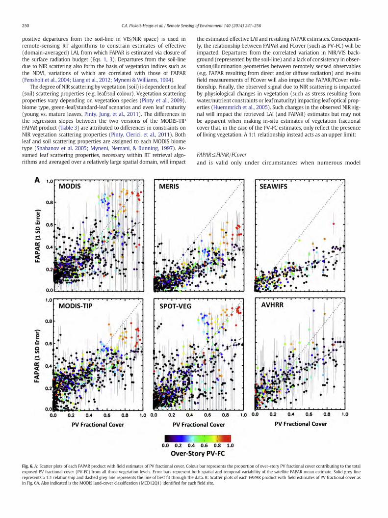
3.2.1. Comparison with in-situ field measurements of PV, NPV and BSFig. 6A plots satellite-derived FAPAR against in-situ estimated vege-

tation fractional cover (specifically PV-FC, see Section 2.2.2). The plottedFAPAR estimates were obtained from the closest single pixel to thereported field-site location. Little discernable difference was observedwhen plotting the average FAPAR estimate from a 3 × 3 pixel-matrixoverlying the field site. Table 3 provides summary statistics of the linearregression between PV-FC and FAPAR (corresponding to the dashedline-of-best-fit in Fig. 6A). No product produces a ~1:1 relationshipbetween FAPAR and PV-FC and all products show different sensitivitiesof FAPAR to PV-FC (coefficient of linear regression in Table 3). Note the

Fig. 2. A: MFC — annual mean FAPAR climatology. B: Mean annual precipitation (mm).

Table 2Spatial correlation between the mean FAPAR climatology (MFC) and precipitationclimatology (Fig. 2) for each drainage division listed in Section 2.2.3 and Fig. 1B.

Drainage division Spatial correlation

North-East Queensland Coast 0.72South-East Australian Coast (NSW/Vic) 0.66Tasmania −0.08Murray–Darling Basin (MDB) 0.82Western Australian Coast 0.82Northern Australia 0.78Central Australia 0.75Western Plateau 0.43Australia 0.73

Fig. 3.Differencemaps between the individual annual FAPAR climatology for eachproductand the mean FAPAR climatology (MFC, Fig. 2A) across all products.

247C.A. Pickett-Heaps et al. / Remote Sensing of Environment 140 (2014) 241–256

difference in sensitivities between the two versions of the MODIS-TIPproduct (Table 3 ), related to the standard-leaf/green-leaf scenarios.All products show differing levels of scatter around the line-of-best-fit(Lin. Reg. SD in Table 3,). Some products (MODIS, MODIS-TIP, AVHRR)show a positive offset in FAPAR within regions of little or no PV fraction(Intercept in Table 3). Other products (MERIS/SeaWiFS/SPOT-VEG)appear on average to correctly identify regions of very low PV-FCwithinspecified uncertainty tolerances of ~0.1 (Gobron, Pinty, Taberner, et al.,2006; Gobron et al., 2008).

Fig. 6A indicates the fraction of over-story (green) vegetation(N2 m) contributing to PV-FC. High proportion of over-story vegetationcover represents field sites in forested biomeswhile the remaining siteslie in regions of significant ground cover (e.g. grassland, savannah,shrubland and agricultural biomes). This stratification clearly identifiestwo groups of field sites with similar estimates of PV-FC but consider-ably different FAPAR estimates from MODIS and SPOT-VEG. Excludingfield sites with over-story fractional cover N0 results in a similar fit tothe in-situ data across all products and no remaining site differentiation(Table 4). SPOT-VEG retains a somewhat higher sensitivity in FAPARwith increases in PV-FC.

Fig. 6B repeats the scatter plots of Fig. 6A but indicates the MODISland-cover biome classification (MDC12Q1) for each field site (seeSection 2.2.3). Similar to Fig. 6A, field sites classified as primarily broad-leaf evergreen generate considerably higher MODIS FAPAR estimatesrelative to other biomes with the same level of PV-FC. Most field siteswith a significant level of over-story PV fractional cover (Fig. 6A) arecorrectly classified as forest. This suggests that, with the availableMDC12Q1 biome classes, land-cover miss-classification across the fieldsites is not a significant problem.

3.2.2. Comparison to the satellite-derived fractional cover productFig. 7A presents the FAPAR time-series for the 6 products in regions

of predominantly PV, NPV and BS. Table 3 provides statistics related tothe time-series presented in Fig. 7A. Fig. 7B presents the number ofgrids where the fractional coverage from the SD-FC product is N80%for PV, NPV and BS. Homogeneous cover in PV and BS frequently occurin coastal regions and central Australia respectively. Areas of homoge-neous NPV occur infrequently in relatively small, contiguous regions.

Fig. 4. Time-series of the different FAPAR satellite products (persistent vegetation component) for Australia and 8 Australian drainage divisions. The plots on the right present the frequen-cy histograms of each product (full FAPAR signal) for each region.

248 C.A. Pickett-Heaps et al. / Remote Sensing of Environment 140 (2014) 241–256

Immediately apparent from Fig. 7A are different base-level FAPARestimates in regions of little or no green vegetation cover (NPV and BStime-series). MERIS, SeaWiFS and SPOT-VEG generate FAPAR estimatesof b0.05 whereas MODIS, MODIS-TIP and AVHRR show a significantpositive offset (Table 3). These offsets are consistent with those appar-ent from comparisons to in-situ PV-FC estimates (Fig. 6, Table 3) andlargely explain why products differ in the semi-arid regions of centralAustralia.

After accounting for offsets in base-level FAPAR, mean FAPAR esti-mates in regions of predominantly PV fractional coverage (green vege-tation) also differ (range in FAPAR in Table 3). SPOT-VEG generates thehighest FAPAR. MERIS/SeaWiFS/MODIS-TIP generate low FAPAR, con-sistent with systematically low FAPAR in regions of dense vegetationcoverage (e.g. SE coast of Australia, Fig. 4).

The differences in FAPAR sensitivity to PV-FC identified in Fig. 7A areconsistent with the differences in sensitivity identified from compari-sons to in-situ field data (Fig. 6, Table 3). The close association betweenin-situ estimated sensitivity and biome type likely extends to a largerspatial scale provided by the SD-FC product, with biome type influenc-ing the range in FAPAR of certain products across Australia (Table 3).MODIS forest biomes (Fig. 6B) occur predominantly in regions of highPV-FC (Fig. 7B). The range in SPOT-VEG FAPAR may also be a result ofglobal rescaling to 0–1 (Baret et al., 2013; Meroni et al., 2012). Therange in FAPAR of the MODIS-TIP GREEN version (Table 3) was foundto be less than that of the STANDARD version. Thus, in addition to

biome type, assumptions related to vegetation scattering properties in-fluence the range in FAPAR across the continent.

A comparison between different backgrounds (BS and NPV) can bemade fromFig. 7B and Table 3,where a positive offset in FAPARbetweena NPV background relative to a BS background may suggest a positivecontribution fromNPVmaterial to a FAPAR signal. However,most prod-ucts exhibit an insignificant difference between the two backgrounds.MODIS-TIP exhibits an unexpected large positive difference betweenBS background relative toNPVbackground. This interesting discrepancyshould be treatedwith caution as it predominantly occurs in small, con-tiguous regions of savanna in northern Australia (Fig. 7B) and is not ap-parent in comparisons with in-situ data (not shown).

4. Discussion

Despite ostensibly significant disagreements, the FAPAR satelliteproducts do show robust spatial and temporal patterns acrossAustralia. Moreover, the disagreements can be partially attributed to aconsistent offset in FAPAR in some products across much of the conti-nent. An offset may be accounted for in certain applications throughproduct-specific model retuning. This likely explains why differentFAPAR products used in biospheric diagnostic models (Haverd et al.,2013; Seixas et al., 2009) generate highly consistent continental meanNPP/NEP estimates but reduced consistency in regional estimates andseasonal variation. The comparison of the FAPAR products to the SD-

Fig. 5. Seasonal climatology plots of the different FAPAR satellite products (recurrent vegetation component) for Australia and 8 Australian drainage divisions. Note: All seasonal plots havebeen adjusted to a common seasonal minimum FAPAR value of 0.01. This aids in comparing the amplitude and timing of the seasonal maximums/minimums and rates of green-up andsenescence. A 1-month moving average smoothing filter has been applied to all seasonal climatologies except AVHRR.

249C.A. Pickett-Heaps et al. / Remote Sensing of Environment 140 (2014) 241–256

FC product is generally consistent with the comparison to the in-situfield estimates of vegetation fractional cover.

Physically consistent in-situ field estimates have been used to vali-date the FAPAR products (Table 5). Fensholt, Sandholt, and Rasmussen(2004) and Huemmrich, Privette, Mukelabai, Myneni, and Knyazikhin(2005) identified a positive bias of ~0.2 inMODIS FAPAR estimates, con-sistent with this study. Gobron, Pinty, Aussedat, et al. (2006), Gobronet al. (2008) estimated the MERIS and SeaWiFS FAPAR uncertainty as~0.1, consistent with the small offsets identified here. As these uncer-tainty estimates are based on relatively fewfield sites, their applicabilityat larger spatial scales and/or within different geographical regions andbiomes may be limited. In addition, the theoretical (or simulated) un-certainty in LAI (and consequently FAPAR) derived from remotely-sensed observations varies non-linearly with LAI (FAPAR) (Myneniet al., 2002; Pinty, Clerici, et al., 2011) and applies to all products. A re-duction in sensitivity of a remotely-sensed signal to increasing LAI upto a point of signal saturation (no sensitivity, Shabanov et al. 2005)leads to a loss of observational constraint and an increase in parameteruncertainty. The point of signal saturation varies depending on theproduct as well as in space and time (Myneni et al., 2002) but typicallyoccurs at an LAI of 3–4 (Pinty, Andredakis, et al., 2011; Pinty, Jung, et al.,2011) for MODIS-TIP and an LAI of ~3.5 for MODIS (Shabanov et al.2005).

Fig. 8 provides an analysis of the a posteriori uncertainty (1.σ) in theMODIS-TIP FAPAR. Minimum FAPAR uncertainty estimates are 0.4–0.5

and correspond to theMODIS-TIP base-level FAPAR estimates describedpreviously. As FAPAR (LAI) increases, uncertainty in FAPAR (LAI) in-creases as expected (up to ~0.8 uncertainty in FAPAR). More surprisingis an increase in FAPAR for very low values of FAPAR (b0.3), a result re-lated to uncertainties in soil background (Pinty, Clerici, et al., 2011). Thepositive offset in base-level MODIS-TIP FAPAR mentioned previously(Figs. 6 and 7B) is consistent with the estimated uncertainty in FAPAR.The Bayesian inversion methodology of MODIS-TIP allows for the prop-agation of a priori uncertainties (e.g. error in observations) through tothe state parameters (LAI, FAPAR), providing a theoretical uncertaintyacross the full range of LAI/FAPAR.

The comparison of satellite-derived FAPAR to in-situ estimatesof PV-FC reveals a relationship as b1:1 for all products concerned (coef-ficient of linear regression range: 0.30–0.57, Table 3). This is in contrastto the expected ~1:1 theoretical sensitivity as shown previously inSection 2.3.2. The linear 1:1 relationship between FAPAR/FIPAR andvegetation FC is appropriate when FAPAR is measured directly. Howev-er, remotely sensed FAPAR is obtained indirectly through closure of thesurface radiation budget, constrained by observed scattering of NIRradiation rather than observed absorption of PAR. Perturbing effects ofthe background albedo within the visible (VIS) spectrum (correspond-ing to PAR) prevent observed changes in VIS albedo (or red BRFs) toestimate FAPAR directly. The linear relationship between changes inVIS and NIR albedo defines a so-called ‘soil-line’ (Chi, 2003) to accountfor changes in background NIR albedo. NIR scattering (illustrated by

250 C.A. Pickett-Heaps et al. / Remote Sensing of Environment 140 (2014) 241–256

positive departures from the soil-line in VIS/NIR space) is used inremote-sensing RT algorithms to constrain estimates of effective(domain-averaged) LAI, from which FAPAR is estimated via closure ofthe surface radiation budget (Eqs. 1, 3). Departures from the soil-linedue to NIR scattering also form the basis of vegetation indices such asthe NDVI, variations of which are correlated with those of FAPAR(Fensholt et al., 2004; Liang et al., 2012; Myneni & Williams, 1994).

The degree ofNIR scattering by vegetation (soil) is dependent on leaf(soil) scattering properties (e.g. leaf/soil colour). Vegetation scatteringproperties vary depending on vegetation species (Pinty et al., 2009),biome type, green-leaf/standard-leaf scenarios and even leaf maturity(young vs. mature leaves, Pinty, Jung, et al., 2011). The differences inthe regression slopes between the two versions of the MODIS-TIPFAPAR product (Table 3) are attributed to differences in constraints onNIR vegetation scattering properties (Pinty, Clerici, et al., 2011). Bothleaf and soil scattering properties are assigned to each MODIS biometype (Shabanov et al. 2005; Myneni, Nemani, & Running, 1997). As-sumed leaf scattering properties, necessary within RT retrieval algo-rithms and averaged over a relatively large spatial domain, will impact

Fig. 6. A: Scatter plots of each FAPAR product with field estimates of PV fractional cover. Colouexposed PV fractional cover (PV-FC) from all three vegetation levels. Error bars represent borepresents a 1:1 relationship and dashed grey line represents the line of best fit through the din Fig. 6A. Also indicated is the MODIS land-cover classification (MCD12Q1) identified for each

the estimated effective LAI and resulting FAPAR estimates. Consequent-ly, the relationship between FAPAR and FCover (such as PV-FC) will beimpacted. Departures from the correlated variation in NIR/VIS back-ground (represented by the soil-line) and a lack of consistency in obser-vation/illumination geometries between remotely sensed observables(e.g. FAPAR resulting from direct and/or diffuse radiation) and in-situfield measurements of FCover will also impact the FAPAR/FCover rela-tionship. Finally, the observed signal due to NIR scattering is impactedby physiological changes in vegetation (such as stress resulting fromwater/nutrient constraints or leafmaturity) impacting leaf optical prop-erties (Huemmrich et al., 2005). Such changes in the observed NIR sig-nal will impact the retrieved LAI (and FAPAR) estimates but may notbe apparent when making in-situ estimates of vegetation fractionalcover that, in the case of the PV-FC estimates, only reflect the presenceof living vegetation. A 1:1 relationship instead acts as an upper limit:

FAPAR≤FIPAR=FCover

and is valid only under circumstances when numerous model

r bar represents the proportion of over-story PV fractional cover contributing to the totalth spatial and temporal variability of the satellite FAPAR mean estimate. Solid grey lineata. B: Scatter plots of each FAPAR product with field estimates of PV fractional cover asfield site.

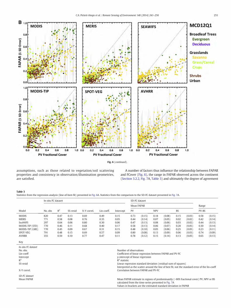
Fig. 6 (continued).

251C.A. Pickett-Heaps et al. / Remote Sensing of Environment 140 (2014) 241–256

assumptions, such as those related to vegetation/soil scatteringproperties and consistency in observation/illumination geometries,are satisfied.

Table 3Statistics from the regression analysis (line-of-best-fit) presented in Fig. 6A. Statistics from the

In-situ FC dataset

Model No. obs R2 SS-resid X-Y correl. Lin-coeff. Inter

MODIS 820 0.47 0.13 0.69 0.49 0.15MERIS 771 0.58 0.08 0.76 0.35 0.05SeaWiFS 297 0.64 0.06 0.80 0.30 0.06MODIS-TIP (STD) 770 0.46 0.11 0.68 0.40 0.17MODIS-TIP (GRE) 770 0.45 0.09 0.67 0.31 0.15SPOT-VEG 791 0.48 0.15 0.69 0.57 0.09AVHRR 355 0.59 0.10 0.77 0.47 0.11

Key

In-situ FC datasetNo. obs. NuLin-coeff CoIntercept y-iR2 R2

SS-resid LinInt

X-Y correl. Co

SD-FC datasetMean FAPAR Me

calVa

A number of factors thus influence the relationship between FAPARand FCover (Fig. 6), the range in FAPAR observed across the continent(Section 3.2.2, Fig. 7A, Table 3) and ultimately the degree of agreement

comparison to the SD-FC dataset presented in Fig. 7A.

SD-FC dataset

Mean FAPAR Range

cept PV NPV BS PV-BS

0.73 (0.15) 0.18 (0.08) 0.15 (0.03) 0.58 (0.15)0.44 (0.14) 0.07 (0.05) 0.02 (0.02) 0.42 (0.14)0.47 (0.13) 0.08 (0.06) 0.03 (0.02) 0.44 (0.13)0.58 (0.13) 0.06 (0.07) 0.28 (0.05) 0.30 (0.14)0.48 (0.10) 0.05 (0.06) 0.25 (0.05) 0.23 (0.11)0.80 (0.08) 0.13 (0.09) 0.06 (0.03) 0.74 (0.09)0.78 (0.12) 0.15 (0.14) 0.13 (0.05) 0.65 (0.13)

mber of observationsefficient of linear regression between FAPAR and PV-FCntercept of linear regressionstatisticear regression standard deviation (residual sum of squares)erpreted as the scatter around the line of best fit, not the standard error of the lin-coeffrrelation between FAPAR and PV-FC

an FAPAR estimate in regions of predominantly (N80% fractional cover) PV, NPV or BSculated from the time-series presented in Fig. 7Alues in brackets are the estimated standard deviation in FAPAR

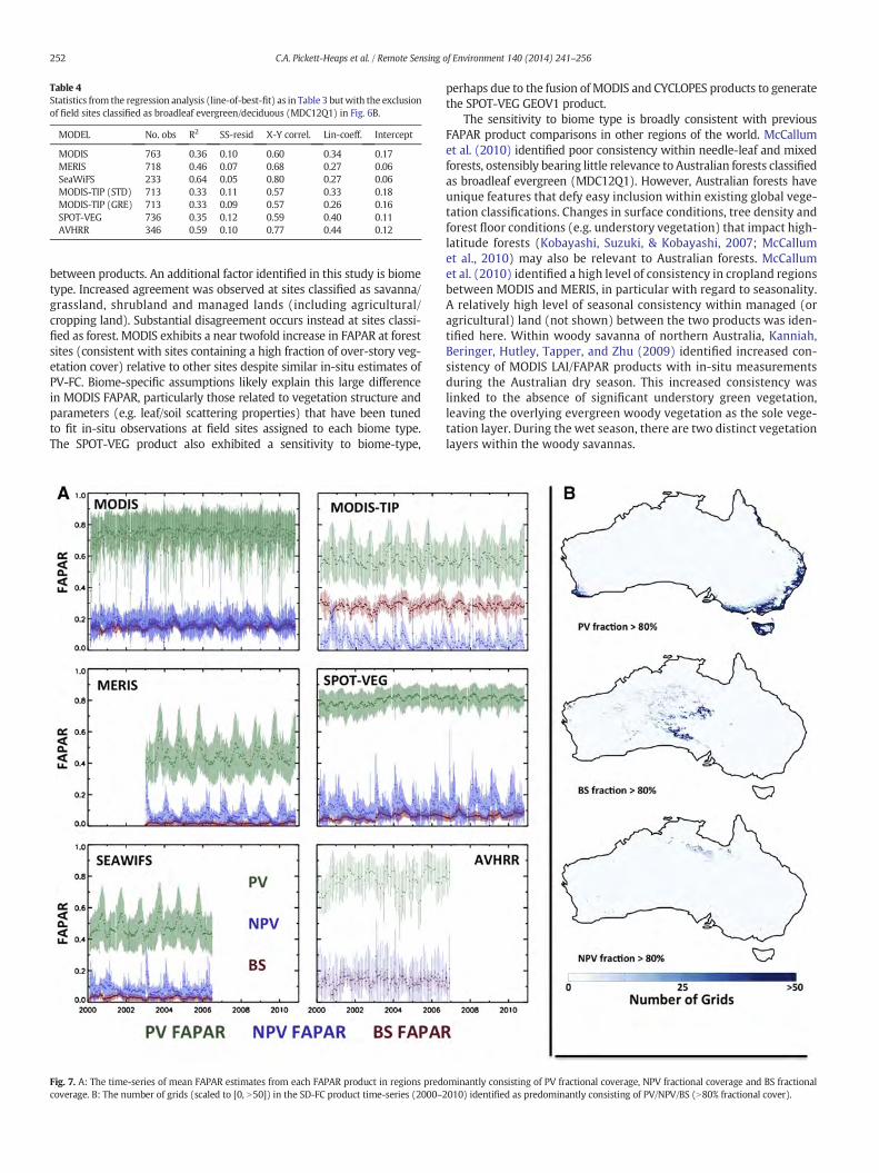
Table 4Statistics from the regression analysis (line-of-best-fit) as in Table 3 butwith the exclusionof field sites classified as broadleaf evergreen/deciduous (MDC12Q1) in Fig. 6B.

MODEL No. obs R2 SS-resid X-Y correl. Lin-coeff. Intercept

MODIS 763 0.36 0.10 0.60 0.34 0.17MERIS 718 0.46 0.07 0.68 0.27 0.06SeaWiFS 233 0.64 0.05 0.80 0.27 0.06MODIS-TIP (STD) 713 0.33 0.11 0.57 0.33 0.18MODIS-TIP (GRE) 713 0.33 0.09 0.57 0.26 0.16SPOT-VEG 736 0.35 0.12 0.59 0.40 0.11AVHRR 346 0.59 0.10 0.77 0.44 0.12

252 C.A. Pickett-Heaps et al. / Remote Sensing of Environment 140 (2014) 241–256

between products. An additional factor identified in this study is biometype. Increased agreement was observed at sites classified as savanna/grassland, shrubland and managed lands (including agricultural/cropping land). Substantial disagreement occurs instead at sites classi-fied as forest. MODIS exhibits a near twofold increase in FAPAR at forestsites (consistent with sites containing a high fraction of over-story veg-etation cover) relative to other sites despite similar in-situ estimates ofPV-FC. Biome-specific assumptions likely explain this large differencein MODIS FAPAR, particularly those related to vegetation structure andparameters (e.g. leaf/soil scattering properties) that have been tunedto fit in-situ observations at field sites assigned to each biome type.The SPOT-VEG product also exhibited a sensitivity to biome-type,

Fig. 7. A: The time-series of mean FAPAR estimates from each FAPAR product in regions predcoverage. B: The number of grids (scaled to [0, N50]) in the SD-FC product time-series (2000–

perhaps due to the fusion of MODIS and CYCLOPES products to generatethe SPOT-VEG GEOV1 product.

The sensitivity to biome type is broadly consistent with previousFAPAR product comparisons in other regions of the world. McCallumet al. (2010) identified poor consistency within needle-leaf and mixedforests, ostensibly bearing little relevance to Australian forests classifiedas broadleaf evergreen (MDC12Q1). However, Australian forests haveunique features that defy easy inclusion within existing global vege-tation classifications. Changes in surface conditions, tree density andforest floor conditions (e.g. understory vegetation) that impact high-latitude forests (Kobayashi, Suzuki, & Kobayashi, 2007; McCallumet al., 2010) may also be relevant to Australian forests. McCallumet al. (2010) identified a high level of consistency in cropland regionsbetween MODIS and MERIS, in particular with regard to seasonality.A relatively high level of seasonal consistency within managed (oragricultural) land (not shown) between the two products was iden-tified here. Within woody savanna of northern Australia, Kanniah,Beringer, Hutley, Tapper, and Zhu (2009) identified increased con-sistency of MODIS LAI/FAPAR products with in-situ measurementsduring the Australian dry season. This increased consistency waslinked to the absence of significant understory green vegetation,leaving the overlying evergreen woody vegetation as the sole vege-tation layer. During the wet season, there are two distinct vegetationlayers within the woody savannas.

ominantly consisting of PV fractional coverage, NPV fractional coverage and BS fractional2010) identified as predominantly consisting of PV/NPV/BS (N80% fractional cover).

Table 5Uncertainty estimates of the FAPAR products based on published comparisons to in-situ observations.

FAPAR product Citation Uncertainty/bias Field site location Field site description

MODIS Fensholt et al. (2004) ~0.2 W Africa (Senegal) Semi-arid grassland and savanna (Sahel)Huemmrich et al. (2005) ~0.2 S Africa (W Zambia) Kalahari woodlandSteinberg, Goetz, and Hyer, (2006) 0.05–0.4 Central Alaska Boreal Forest

MERIS Gobron, Pinty, Taberner, et al. (2006),Gobron, Pinty,Aussedat, et al., 2006; Gobron et al., 2008)

0.1 Various Various (grassland/savanna, forest, cropland)

SeaWiFS Gobron, Pinty, Aussedat, et al. (2006) 0.1 Various Various (grassland/savanna, forest, cropland)MODIS-TIP (STD) Pinty, Jung, et al. (2011) 0.15 Central Germany Deciduous European forestSPOT-VEG Camacho, Cernicharo, Lacaze, Baret, and Weiss (2013) 0.1 Not specified Not specifiedAVHRR Not available (N/A) N/A N/A N/A

253C.A. Pickett-Heaps et al. / Remote Sensing of Environment 140 (2014) 241–256

A result consistent with previous studies (McCallum et al., 2010;Pinty et al., 2008; Seixas et al., 2009) is a systematic difference betweenthe MODIS and MERIS/SeaWiFS FAPAR products, identified here as aresult of both a systematic offset in base-level FAPAR and sensitivity tobiome type. Pinty et al. (2008) found that MODIS significantly over-estimated FAPAR relative to MERIS/SeaWiFS andMODIS-TIP at two for-ested sites (needle-leaf evergreen, needle-leaf deciduous) that experi-ence snow cover during the northern-hemisphere winter. MODIS wasnot found to overestimate FAPAR at an additional forest site (broad-leaf deciduous). A SPOT-VEG derived product using the same algorithmas the MERIS product included in this study was also found to routinelyunderestimate FAPAR relative to the SPOT-VEGGEOV1 product (Meroniet al., 2012). This suggests that perhaps the algorithms employed ratherthan differences in instrumentation have greater influence on the de-gree of dissimilarity between products. Supporting this argument isthe high level of agreement between the MERIS and SeaWiFS productsobserved here and elsewhere (Gobron, Belward, Pinty, & Knorr, 2010;Gobron, Pinty, Taberner, et al., 2006). Both products are based on thesame algorithm but use sensor-specific parameter tuning.

5. Summary and conclusions

The evaluation of six global FAPAR satellite products across Australiahighlights significant disagreement amongst the products, albeit dis-playing robust spatial and temporal patterns. These disagreements are

Fig. 8.A:Relationship betweenMODIS-TIP FAPAR and the a posteriori uncertainty in FAPAR (1.σthe a posteriori uncertainty in effective LAI (1.σ). PV-FC indicated by the colour scale. C: Relatiodicated by colour scale.

spatially heterogeneous, resulting in no single product identifiedroutinely as an outlier. These disagreements also result in differencesin seasonal variation.

The findings in this study can be summarized as follows:

- Systematic differences in (1) base-level FAPAR estimates and (2)FAPAR sensitivity to spatio-temporal changes in vegetation coverare themain features of thedifferences between the FAPARproducts.

- Differences in FAPAR sensitivity to increases in vegetation cover canbe attributed in part to changes in biome type (and model assump-tions therein) but are also likely related to other factors such as theassumed scattering properties of vegetation in the NIR.

- Differences between products depend on biome type, particularly ifsystematic differences in base-level FAPAR are accounted for. Rela-tively high agreement across the products occurs within savanna/grassland, shrubland andmanaged land (agricultural land) classifiedbiomes. Particularly high disagreement occurs within forest-classifiedbiomes.

- Differences between products that depend on biome type are appar-ent at the large-scale, when compared to the SD-FC product or usinga stratificationmodel defining different vegetation types. Suchdiffer-ences are consistent at the small-scale, when compared to in-situestimated vegetation fractional (FC-dataset).

- A comparison between satellite-derived FAPAR and in-situ estimatedvegetation fractional cover reveals a relationship b1:1 for all FAPARsatellite products. Reasons for this can be attributed to:

). PV-FC indicated by the colour scale. B: Relationship betweenMODIS-TIP effective LAI andnship betweenMODIS-TIP FAPAR and PV-FC. A posteriori uncertainties in FAPAR (1.σ) in-

Over-story Mid-story Ground-cover:

FCeff,i,L3 = FCi. L3

FCT ;L3 ¼ ∑2

i¼1FCi;L3

FCE;i ¼ ∑3

L¼1FCeff ;i;L

∑3

i¼1FCE;i ¼ 1

FCeff,i,L2 = FCi,L2 ⋅(1 − FT,L3)

FCT;L2 ¼ ∑2

i¼1FCi;L2

FCeff,i,L1 = FCi,L1 ⋅ (1 − FT,L3) ⋅(1 − FT,L2)

254 C.A. Pickett-Heaps et al. / Remote Sensing of Environment 140 (2014) 241–256

⁎ Sensitivity in the assumed NIR scattering properties of vegetation⁎ Departures from the collinearity in background albedo (reflectance)in the VIS and NIR spectrums

⁎ Lack of consistency between the definitions of FAPAR as it applies toeach satellite product and the estimation of in-situ fractional cover

⁎ Physiological characteristics (and changes) in vegetation (such asstress-induced changes) that impact the observed NIR scatteringsignal generated by vegetation butmaynot be apparentwhenmak-ing in-situ field estimates.

Acknowledgements

The authors would like to acknowledge the Australian Climate ChangeScience Program (ACCSP) for supporting this work. ACCSP is a programmeof the Commonwealth Science and Industrial Research Organisation(CSIRO), the Bureau of Meteorology and the Department of ClimateChange and Energy Efficiency. The Office of the Chief Executive (CSIRO)also provided financial support in the form of a post-doctoral fellowship.

The authors would like to acknowledge the custodians of the fielddata of fractional cover used in this study.

We acknowledge the use of the SLATS field data obtained from theQueensland State Government (Department of Environment and Re-source Management) and that our study is:

“Based on or contains data provided by the State of Queensland(Department of Environment and Resource Management) [2010]. Inconsideration of the State permitting use of this data you acknowledgeand agree that the State gives no warranty in relation to the data(including accuracy, reliability, completeness, currency or suitability)and accepts no liability (including without limitation, liability in negli-gence) for any loss, damage or costs (including consequential damage)relating to any use of the data. Data must not be used for direct market-ing or be used in breach of the privacy laws.”

We acknowledge the use of the Australian ground cover referencesites database:

ABARES (2012) Ground cover reference sites database. AustralianBureau of Agricultural and Resource Economics and Sciences, Canberra,Australia. https://rs.nci.org.au/FcSiteData/

We further acknowledge the Australian state government agenciesproviding support in the collection of field data contributing to theAustralian ground cover reference sites database

The authors would also like to acknowledge the assistance providedbyDr. Juan-Pablo Guerschman (CSIRO–L&W), Dr. Peter Scarth (Univ.Queensland) and Ms. Jasmine Rickards (ABARES).

The authors would like to acknowledge the provision of the MODISand AVHRR FAPAR and satellite-derived fractional cover satellite prod-ucts used in this study. These datasets, and associated processing, wereprovided by:

The AusCover Facility, Terrestrial Ecosystem Research Networkhttp://data.auscover.org.au/

Paget and King (2008) MODIS Land data sets for the Australian region.CSIRO Marine and Atmospheric Research Internal Report No. 004.https://lpdaac.usgs.gov/lpdaac/products/modis_policies

The authors would like to acknowledge the provision of theMERIS, SeaWiFS and MODIS-TIP FAPAR products used in this study.We acknowledge the Joint Research Center of the European Commis-sion (EC–JRC–2011). These datasets, and associated processing, wereprovided by:

The SOLO (Action 24004) of EC-IES using the Joint Research Centerprocessing chain for SeaWiFS and the European Space Grid OnDemand Facility (http://gpod.eo.esa.int/) for MERIS, respectively.EC–JRC–2011: http://fapar.jrc.ec.europa.eu/

In regard to the SeaWiFS data:

“The data were possible thanks to the SeaWiFS Project (Code 970.2)and the Goddard Earth Sciences Data and Information ServicesCenter/Distributed Active Archive Center (Code 902) at the GoddardSpace Flight Center, Greenbelt, MD 20771, for the production anddistribution of these data, respectively. These activities are spon-sored by NASA's Earth Science Enterprise.

All SeaWiFS scenes (full resolution Local Area Coverage images andsub-sampled Global Area Coverage images) covering the study areahave been processed and subsequently mapped with a nearestneighbor technique on a 2-km resolution regular grid, as explainedin Mélin, Steinich, Gobron, Pinty, and Verstraete, (2002).”

The authors would like to acknowledge the provision of the SPOT-VEG FAPAR product used in this study:

“The research leading to these results has received funding from theEuropean Community's Seventh Framework Program (FP7/2007–2013) under grant agreement no 218795. These products are the jointproperty of INRA, CNES, and VITO under copyright geoland2. They aregenerated from the SPOT VEGETATION data under copyright CNES anddistribution by VITO.”

The authors acknowledge the GeoLand2 data portal for access to theSPOT-VEG FAPAR product: http://www.geoland2.eu/ and the assistanceprovided by the GeoLand2 helpdesk.

Appendix A

In-situ estimates of vegetation fractional cover have been obtainedat ~600 field sites across Australia (Fig. 1A). The fractional cover datasetconsists of ~800 separate estimates. Each field site measures approxi-mately 100 m × 100 m (1 ha), within which fractional cover estimatesat three vegetation levels are obtained. The sampling strategy (Muiret al., 2011; Rickards, Stewart, Randall, & Bordas, 2012) consists of de-termining the presence/absence of either PV, NPV or BS along a transectat 1 m intervals for each vegetation level. Eight transects are defined ina symmetric star orientation radiating out from the centre of the fieldsite. The ratio between the total counts of PV, NPV and BS respectivelyand the total number of samples taken represents the fractional coverof PV, NPV and BS for each vegetation level at the field site.

The FC estimates from the three vegetation levels must be combinedto estimate the total exposed PV/NPV/BS fractional cover apparent fromabove the canopy. The exposed fraction is calculated by scaling the frac-tional cover estimates at a particular vegetation level by the ‘uncoveredfraction’ of the vegetation level(s) above. The exposed fractional coverof PV/NPV/BS at each level and the total PV/NPV/BS fractional cover forthe site (FCE,i) are calculated as follows:

255C.A. Pickett-Heaps et al. / Remote Sensing of Environment 140 (2014) 241–256

Where:

FCi,L Fractional cover at level L and veg. type iFCeff,i,L Effective fractional cover at level L and veg. type iFCT,L Total vegetation cover (PV & NPV) at level LL Canopy level (1: ground cover, 2: mid-story, 3: over-story)i Vegetation type (1: PV, 2: NPV, 3: BS)FCE,i Total exposed cover for vegetation type i

Appendix B

The split of the full FAPAR signal into the recurrent and persistentcomponents follows algorithms developed by Donohue et al. (2009),Lu et al. (2003) and Roderick et al. (1999). The algorithm, as describedby Donohue et al. (2009) is outlined as follows:

- Data dropouts (erroneous FAPAR values) are identified and re-moved. The difference (dt) between a FAPAR estimate, ft at time t,and themean FAPAR estimate (fm)within a 1–3 monthmovingwin-dow centred on time t and excluding ftwas calculated. If dt exceeded0.1, ft is flagged as a dropout and replaced by fm. A decrease of 0.1FAPAR over one time-step is realistic if this decrease is maintainedin successive time-steps. However, such a decrease followed by anequally large increase (recovery) is unrealistic and thus can beflagged as an erroneous dropout. The size of the 1–3 month movingwindow is dependent on the time-resolution of the satellite data.

- A 7-month moving minimum is applied to the FAPAR time-serieswith the FAPAR dropouts removed (Fp1).

- A 9-month moving average is applied to the Fp1 time-series (Fp2).- A preliminary recurrent component is calculated:

Fr1 ¼ Ft–Fp2

- The following condition is then applied to obtain the persistentFAPAR component:

If Fr1b0; then Fp ¼ Fp2– Fr1j j

If Fr1N0; then Fp ¼ Fp2

- Fp represents the final persistent component. The final recurrentcomponent is calculated from the original time-series (Ft, dropoutsremoved) as follows:

Fr ¼ Ft–Fp

Annual and seasonal climatologies of all FAPAR products (andpersistent/recurrent components) were generated. Climatologies overa common time-period for all products (2003–2006)were also calculat-ed and compared, with little difference identified between the two setsof climatologies.

Appendix C

The theoretical relationship between FAPAR and PV-FC was derivedby simulating both quantities using the CanSPART radiative transfermodel (Haverd et al., 2012; Lovell et al., 2012): amodel of gap probability(including canopy structure effects), coupled to a modified two-streamradiative transfer scheme. CANSPART has been widely tested againstother canopy structure models and above-canopy reflectances (Haverdet al., 2012), and against ground-based LIDAR observations of gap prob-ability (Lovell et al., 2012). The range of sensitivities was obtained asthe range from simulations representing extreme vegetation structure(unclumped to highly clumped) and leaf scattering coefficients. Specifi-cally, simulations were performed for leaf area indices ranging from 0.2

to 5with: (i) intermediate clumping (790 stemsha-1); (ii) high clumping(200 stems ha-1); (iii) no clumping (horizontally homogeneousvegetation) and (iv) extreme values (+2 s.d.) of leaf scattering coef-ficients; and (v) vertical leaf angle distribution (instead of spherical).Mean leaf scattering coefficients and their variability were derived froman ensemble of 50 PROSPECT (Jacquemoud & Baret, 1990) simulationsfor Eucalyptus leaves, with input parameter values randomly drawnfrom sampleswithmean and standard deviation derived from literaturevalues (Barry, Newnham, & Stone, 2009; Datt, 1998, 1999).

References

Bacour, C., Baret, F., Beal, D., Weiss, M., & Pavageau, K. (2006). Neural network estimationof LAI, fAPAR, fCover and LAI x Cab, from top of canopy MERIS reflectance data: Prin-ciples and validation. Remote Sensing of Environment, 105(4), 313–325.

Baret, F., Hagolle, O., Geiger, B., Bicheron, P., Miras, B., Huc, M., et al. (2007). LAI, fAPAR andfCover CYCLOPES global products derived from VEGETATION: Part 1: Principles of thealgorithm. Remote Sensing of Environment, 110(3), 275–286.

Baret, F., Weiss, M., Lacaze, R., Camacho, F., Makhamara, H., Pacholcyzk, P., & Smets, B.(2013). GEOV1: LAI and FAPAR essential climate variables and FCOVER globaltime-series capitalizing over existing products. Part 1: Principles of developmentand production. Remote Sensing of Environment, 137, 299–309.

Barry, K. M., Newnham, G. J., & Stone, C. (2009). Estimation of chlorophyll content ineucalyptus globulus foliage with the leaf reflectance model PROSPECT. Agriculturaland Forest Meteorology, 149(6), 1209–1213.

Boening, C., Willis, J. K., Landerer, F. W., Nerem, R. S., & Fasullo, J. (2012). The 2011 LaNina: So strong, the oceans fell. Geophysical Research Letters, 39, L19602.

Camacho, F., Cernicharo, J., Lacaze, R., Baret, F., & Weiss, M. (2013). GEOV1: LAI, FAPARessential climate variables and FCOVER global time-series capitalizing over existingproducts. Part 2: Validation and intercomparison with reference products. RemoteSensing of Environment, 37, 310–329.

Chi, H. (2003). Practical atmospheric correction of NOAA-AVHRR data using the bare-sandsoil line method. International Journal of Remote Sensing, 24(17), 3369–3379.

Daniell, T. M. (2009). The implications of a decade of drought in Australia (1996–2007).Sécheresse, 20(1), 171–180.

Datt, B. (1998). Remote sensing of chlorophyll a, chlorophyll b, chlorophyll a + b, andtotal carotenoid content in eucalyptus leaves. Remote Sensing of Environment, 66(2),111–121.

Datt, B. (1999). Remote sensing of water content in Eucalyptus leaves. Australian Journalof Botany, 47(6), 909–923.

Donohue, R. J., McVicar, T. I. M., & Roderick, M. L. (2009). Climate-related trends inAustralian vegetation cover as inferred from satellite observations, 1981–2006.Global Change Biology, 15(4), 1025–1039.

Donohue, R. J., Roderick, M. L., & McVicar, T. R. (2008). Deriving consistent long-termvegetation information from AVHRR reflectance data using a cover-triangle-basedframework. Remote Sensing of Environment, 112(6), 2938–2949.

FAO (2008). Development of standards for essential climate variables: Fractionof Absorbed Photosynthetically Active Radiation (FAPAR), Version 8. Availableat: http://www.fao.org/gtos/pubs.html

Fasullo, J. T., Boening, C., Landerer, F. W., & Nerem, R. S. (2013). Australia's unique influ-ence on global sea level in 2010–2011. Geophysical Research Letters, 40(1–6), http://dx.doi.org/10.1002/grl.50834.

Fensholt, R., Sandholt, I., & Rasmussen, M. S. (2004). Evaluation of MODIS LAI, fAPAR andthe relation between fAPAR and NDVI in a semi-arid environment using in situ mea-surements. Remote Sensing of Environment, 91(3), 490–507.

Field, C. B., Randerson, J. T., & Malmström, C. M. (1995). Global net primary production:Combining ecology and remote sensing. Remote Sensing of Environment, 51(1), 74–88.

Fraction of absorbedphotosynthetically active radiationbygreen vegetation. Liang, S., Li, X.,& Wang, J. (Eds.). (2012). Advanced remote sensing: Terrestrial information extractionand applications (pp. 383–414). Oxford, UK: Elsevier Inc.

GCOS (2006). Systematic observation requirements for satellite-based products for climate:GCOS, 107 (90 pp.).

Gitelson, A. A., Gritz, Y., & Merzlyak, M. N. (2003). Relationships between leaf chlorophyllcontent and spectral reflectance and algorithms for non-destructive chlorophyllassessment in higher plant leaves. Journal of Plant Physiology, 160(3), 271–282.

Gobron, N., Belward, A., Pinty, B., & Knorr, W. (2010). Monitoring biosphere vegetation1998–2009. Geophysical Research Letters, 37(15), L15402.

Gobron, N., Pinty, B., Aussedat, O., Chen, J. M., Cohen, W. B., Fensholt, R., et al. (2006b).Evaluation of fraction of absorbed photosynthetically active radiation products fordifferent canopy radiation transfer regimes: Methodology and results using joint re-search center products derived from SeaWIFS against ground-based estimations.Journal of Geophysical Research, 111(D13), D13110.

Gobron, N., Pinty, B., Aussedat, O., Taberner, M., Faber, O., Mélin, F., et al. (2008). Uncer-tainty estimates for the FAPAR operational products derived from MERIS — Impactof top-of-atmosphere radiance uncertainties and validation with field data. RemoteSensing of Environment, 112(4), 1871–1883.

Gobron, N., Pinty, B., Mélin, F., Taberner, M., Verstraete, M. M., Robustelli, M., et al. (2007).Evaluation of the MERIS/ENVISAT FAPAR product. Advances in Space Research, 39(1),105–115.

Gobron, N., Pinty, B., Taberner, M., Mélin, F., Verstraete, M. M., & Widlowski, J. L. (2006a).Monitoring the photosynthetic activity of vegetation from remote sensing data.Advances in Space Research, 38(10), 2196–2202.

256 C.A. Pickett-Heaps et al. / Remote Sensing of Environment 140 (2014) 241–256

Gobron, N., Pinty, B., Verstraete, M. M., & Govaerts, Y. (1997). A semidiscrete model forthe scattering of light by vegetation. Journal of Geophysical Research-Atmospheres,102(D8), 9431–9446.

Gobron, N., Pinty, B., Verstraete, M., & Govaerts, Y. (1999). The MERIS global vegetationindex (MGVI): Description and preliminary application. International Journal ofRemote Sensing, 20(9), 1917–1927.

Gobron, N., Pinty, B., Verstraete, M. M., & Taberneret, M. (2002). VEGETATION, anoptimised FAPAR algorithm theoretical basis document. JRC Publication EUR 20146EN. Luxembourg, UK: Publication Office European Union.

Gobron, N., Pinty, B., Verstraete, M. M., & Widlowski, J. L. (2000). Advanced vegetation in-dices optimized for up-coming sensors: Design, performance, and applications. IEEETransactions on Geoscience and Remote Sensing, 38(6), 2489–2505.

Guerschman, J. P., Hill, M. J., Renzullo, L. J., Barrett, D. J., Marks, A. S., & Botha, E. J. (2009).Estimating fractional cover of photosynthetic vegetation, non-photosynthetic vegeta-tion and bare soil in the Australian tropical savanna region upscaling the EO-1 hype-rion and MODIS sensors. Remote Sensing of Environment, 113(5), 928–945.

Haverd, V., Lovell, J. L., Cuntz, M., Jupp, D. L. B., Newnham, G. J., & Sea, W. (2012). TheCanopy Semi-analytic Pgap And Radiative Transfer (CanSPART) model: Formulationand application. Agricultural and Forest Meteorology, 160, 14–35.

Haverd, V., Raupach, M. R., Briggs, P. R., Canadell, J. G., Isaac, P., Pickett-Heaps, C., et al.(2013). Multiple observation types reduce uncertainty in Australia's terrestrial carbonand water cycles. Biogeosciences, 10, 2011–2040.

Huemmrich, K. F., Privette, J. L., Mukelabai, M., Myneni, R. B., & Knyazikhin, Y. (2005).Time-series validation of MODIS land biophysical products in a Kalahari woodland,Africa. International Journal of Remote Sensing, 26(19), 4381–4398.

Jacquemoud, S., & Baret, F. (1990). PROSPECT: A model of leaf optical properties spectra.Remote Sensing of Environment, 34(2), 75–91.

Jung, M., Verstraete, M., Gobron, N., Reichstein, M., Papale, D., Bondeau, A., et al. (2008).Diagnostic assessment of European gross primary production. Global Change Biology,14(10), 2349–2364.

Kaminski, T., Knorr, W., Scholze, M., Gobron, N., Pinty, B., Giering, R., et al. (2012). Consis-tent assimilation of MERIS FAPAR and atmospheric CO2 into a terrestrial vegetationmodel and interactive mission benefit analysis. Biogeosciences, 9(8), 3173–3184.

Kanniah, K. D., Beringer, J., Hutley, L. B., Tapper, N. J., & Zhu, X. (2009). Evaluation ofcollections 4 and 5 of the MODIS gross primary productivity product and algorithmimprovement at a tropical savanna site in northern Australia. Remote Sensing ofEnvironment, 113(9), 1808–1822.

Kilinc, M., Beringer, J., Hutley, L. B., Haverd, V., & Tapper, N. (2012). An analysis of the sur-face energy budget above theworld's tallest angiosperm forest. Agricultural and ForestMeteorology, 166, 23–31.

Knorr, W., Kaminski, T., Scholze, M., Gobron, N., Pinty, B., Giering, R., et al. (2010). Carboncycle data assimilation with a generic phenology model. Journal of GeophysicalResearch: Biogeosciences, 115(G4), 2005–2012.

Knyazikhin, Y., Glassy, J., Privette, J. L., Tian, Y., Lotsch, A., Zhang, Y., et al. (1999). MODISleaf area index (LAI) and fraction of photosynthetically active radiation absorbed by veg-etation (FPAR) product (MOD15) algorithm theoretical basis document. Theoreticalbasis document. Greenbelt, MD, 20771: NASA Goddard Space Flight Center.

Knyazikhin, Y., Martonchik, J. V., Myneni, R. B., Diner, D. J., & Running, S. W. (1998). Syn-ergistic algorithm for estimating vegetation canopy leaf area index and fraction ofabsorbed photosynthetically active radiation from MODIS and MISR data. Journal ofGeophysical Research, 103(D24), 32257–32276.

Kobayashi, H., Suzuki, R., & Kobayashi, S. (2007). Reflectance seasonality and its relationto the canopy leaf area index in an Eastern Siberian larch forest: Multi-satellite dataand radiative transfer analyses. Remote Sensing of Environment, 106(2), 238–252.

Leuning, R., Cleugh, H. A., Zegelin, S. J., & Hughes, D. (2005). Carbon and water fluxes overa temperate Eucalyptus forest and a tropical wet/dry savanna in Australia: Measure-ments and comparison with MODIS remote sensing estimates. Agricultural and ForestMeteorology, 129, 151–173.

Lovell, J. L., Haverd, V., Jupp, D. L. B., & Newnham, G. J. (2012). The Canopy Semi-AnalyticPGap And Radiative Transfer (CanSPART) model. Part 2. Validation using ground-based LIDAR. Agricultural and Forest Meteorology, 158, 1–12.

Lu, H., Raupach, M. R., McVicar, T. R., & Barrett, D. J. (2003). Decomposition of vegetationcover into woody and herbaceous components using AVHRR NDVI time series.Remote Sensing of Environment, 86(1), 1–18.

McCallum, I., Wagner, W., Schmullius, C., Shvidenko, A., Obersteiner, M., Fritz, S., et al.(2010). Comparison of four global FAPAR datasets over Northern Eurasia for theyear 2000. Remote Sensing of Environment, 114(5), 941–949.

McGrath, G. S., Sadler, R., Fleming, K., Tregoning, P., Hinz, C., & Veneklaas, E. J. (2012).Tropical cyclones and the ecohydrology of Australia's recent continental-scaledrought. Geophysical Research Letters, 39(3), L03404.

Meroni, M., Atzberger, C., Vancutsem, C., Gobron, N., Baret, F., Lacaze, R., et al. (2012).Evaluation of agreement between space remote sensing SPOT-VEGETATION fAPARtime series. IEEE Transactions on Geoscience and Remote Sensing, 51(4), 1951–1962.

Mélin, F., Steinich, C., Gobron, N., Pinty, B., & Verstraete, M. M. (2002). Optimal merging of LACand GAC data from SeaWiFS. International Journal of Remote Sensing, 23(4), 801–807.

Muir, J., Schmidt, M., Tindall, D., Trevithick, R., Scarth, P., & Stewart, J. B. (2011).Field measurement of fractional ground cover: a technical handbook supporting groundcovermonitoring for Australia. Canberra: Queensland Department of Environmentand Resource Management for the Australian Bureau of Agricultural andResource Economics and Sciences (Available at: http://adl.brs.gov.au/data/warehouse/pe_hbgcm9abll07701/HndbkGrndCovMontring2011_1.0.0_LR.pdf)

Murphy, B. F., & Timbal, B. (2008). A review of recent climate variability and climatechange in southeastern Australia. International Journal of Climatology, 28(7), 859–879.

Myneni, R. B., Hoffman, S., Knyazikhin, Y., Privette, J. L., Glassy, J., Tian, Y., et al. (2002).Global products of vegetation leaf area and fraction absorbed PAR from year one ofMODIS data. Remote Sensing of Environment, 83(1), 214–231.

Myneni, B., Nemani, R. R., & Running, S. (1997). Estimation of global leaf area index andabsorbed PAR using radiative transfer models. IEEE Transactions on Geoscience andRemote Sensing, 35(6), 1380–1393.

Myneni, R. B., & Williams, D. L. (1994). On the relationship between FAPAR and NDVI.Remote Sensing of Environment, 49(3), 200–211.

National Climate Centre, Bureau of Meteorology (2012). Australia's wettest two-year pe-riod on record: 2010-2011. Special Climate Statement, 38 available at: http://www.bom.gov.au/climate/current/statements/scs38.pdf.

NLWRA: National Land and Water Resources Audit (2000). Australian Agriculture Assess-ment 2000. Canberra, Australia: Commonwealth of Australia (160 pp.).

NLWRA: National Land and Water Resources Audit (2001). Australian Agriculture Assess-ment 2001. Canberra, Australia: Commonwealth of Australia (480 pp.).

NVIS: Australia's native vegetation (2007). A summary of Australia's major vegetationgroups: Department of Sustainability, Environment, Water, Population and Commu-nities, Commonwealth of Australia, 42.

Paget, M. J., & King, E. A. (2008). MODIS land data sets for the Australian region. CSIROMarine and Atmospheric Research Internal Report No. 004 available at: https://remote-sensing.nci.org.au/u39/public/html/modis/lpdaac-mosaics-cmar/doc/ModisLand_PagetKing_20081203-final.pdf.

Pinty, B., Andredakis, I., Clerici, M., Kaminski, T., Taberner, M., Verstraete, M. M., et al.(2011a). Exploiting the MODIS albedos with the two-stream inversion package(JRC-TIP): 1. Effective leaf area index, vegetation, and soil properties. Journal ofGeophysical Research, 116(D9), D09105.

Pinty, B., Clerici, M., Andredakis, I., Kaminski, T., Taberner, M., Verstraete, M. M., et al.(2011b). Exploiting the MODIS albedos with the two-stream inversion package(JRC-TIP): 2. Fractions of transmitted and absorbed fluxes in the vegetation and soillayers. Journal of Geophysical Research, 116(D9), D09106.

Pinty, B., Jung, M., Kaminski, T., Lavergne, T., Mund, M., Plummer, S., et al. (2011c). Eval-uation of the JRC-TIP 0.01 products over a mid-latitude deciduous forest site.Remote Sensing of Environment, 115(12), 3567–3581.

Pinty, B., Lavergne, T., Dickinson, R. E., Widlowski, J. L., Gobron, N., & Verstraete, M. M.(2006). Simplifying the interaction of land surfaces with radiation for relating remotesensing products to climate models. Journal of Geophysical Research, 111(D2), D02116.

Pinty, B., Lavergne, T., Kaminski, T., Aussedat, O., Giering, R., Gobron, N., et al. (2008).Partitioning the solar radiant fluxes in forest canopies in the presence of snow.Journal of Geophysical Research, 113(D4), D04104.

Pinty, B., Lavergne, T., Voßbeck, M., Kaminski, T., Aussedat, O., Giering, R., et al. (2007). Re-trieving surface parameters for climate models from moderate resolution imagingspectroradiometer (MODIS)-multiangle imaging spectroradiometer (MISR) albedoproducts. Journal of Geophysical Research, 112(D10), D10116.

Pinty, B., Lavergne, T., Widlowski, J. L., Gobron, N., & Verstraete, M.M. (2009). On the needto observe vegetation canopies in the near-infrared to estimate visible light absorp-tion. Remote Sensing of Environment, 113(1), 10–23.

Potter, C. S., Randerson, J. T., Field, C. B., Matson, P. A., Vitousek, P.M., Mooney, H. A., et al.(1993). Terrestrial ecosystem production: A process model based on global satelliteand surface data. Global Biogeochemical Cycles, 7(4), 811–841.

Rickards, J., Stewart, J., Randall, L., & Bordas, V. (2012). Australian ground cover referencesites database: User guide for postGIS: Australian Bureau of Agricultural and ResourceEconomics and Sciences (ABARES), Department of Agriculture, Fisheries and Forestry,Commonwealth of Australia.

Roderick, M. L., Noble, I. R., & Cridland, S. W. (1999). Estimating woody and herba-ceous vegetation cover from time series satellite observations. Global Ecology andBiogeography, 8(6), 501–508.

Seixas, J., Carvalhais, N., Nunes, C., & Benali, A. (2009). Comparative analysis of MODIS-FAPAR and MERIS-MGVI datasets: Potential impacts on ecosystem modeling. RemoteSensing of Environment, 113(12), 2547–2559.

Sellers, P. J. (1985). Canopy reflectance, photosynthesis and transpiration. InternationalJournal of Remote Sensing, 6(8), 1335–1372.

Sellers, P. J. (1987). Canopy reflectance, photosynthesis, and transpiration, II. The role ofbiophysics in the linearity of their interdependence. Remote Sensing of Environment,21(2), 143–183.

Sellers, P. J., Berry, J. A., Collatz, G. J., Field, C. B., & Hall, F. G. (1992). Canopy reflectance,photosynthesis, and transpiration. III. A reanalysis using improved leaf models anda new canopy integration scheme. Remote Sensing of Environment, 42(3), 187–216.

Sellers, P. J., Dickinson, R. E., Randall, D. A., Betts, A. K., Hall, F. G., Berry, J. A., et al. (1997).Modeling the exchanges of energy, water, and carbon between continents and the at-mosphere. Science, 275(5299), 502–509.

Shabanov, N. V., Huang, D., Yang, W., Tan, B., Knyazikhin, Y., Myneni, R. B., Ahl, D. E.,Gower, S. T., & Huete, A. R. (2005). Analysis and optimization of the MODIS leafarea index algorithm retrievals over broadleaf forests. IEEE Transactions onGeoscience and Remote Sensing, 43(8), 1855–1865.

Steinberg, D. C., Goetz, S. J., & Hyer, E. J. (2006). Validation of MODIS F-PAR products in borealforests of Alaska. IEEE Transactions on Geoscience and Remote Sensing, 44(7), 1818–1828.

Tarantola, A. (2005). Inverse problem theory and methods for model parameter estimation.Philadelphia, PA, USA: Society for Industrial and Applied Mathematics.

Ummenhofer, C. C., England, M. H., McIntosh, P. C., Meyers, G. A., Pook, M. J., Risbey, J. S.,et al. (2009). What causes southeast Australia's worst droughts? Geophysical ResearchLetters, 36(4).

Verhoef, W. (1984). Light scattering by leaf layers with application to canopy reflectancemodeling: The SAIL model. Remote Sensing of Environment, 16(2), 125–141.

Vermote, E. F., Tanré, D., Deuze, J. L., Herman, M., & Morcette, J. -J. (1997). Second simula-tion of the satellite signal in the solar spectrum, 6S: An overview. IEEE Transactions onGeoscience and Remote Sensing, 35(3), 675–686.

Widlowski, J. L., Pinty, B., Lavergne, T., Verstraete, M. M., & Gobron, N. (2005). Using 1-Dmodels to interpret the reflectance anisotropy of 3-D canopy targets: Issues andcaveats. IEEE Transactions on Geoscience and Remote Sensing, 43(9), 2008–2017.