Remote Sens. OPEN ACCESS remote sensing · Richard Müller *, Uwe Pfeifroth , Christine...
35
Remote Sens. 2015, 7, 8067-8101; doi:10.3390/rs70608067 OPEN ACCESS remote sensing ISSN 2072-4292 www.mdpi.com/journal/remotesensing Article Digging the METEOSAT Treasure—3 Decades of Solar Surface Radiation Richard Müller *, Uwe Pfeifroth , Christine Träger-Chatterjee, Jörg Trentmann and Roswitha Cremer Deutscher Wetterdienst, Frankfurter Str. 135, D-60387 Offenbach, Germany; E-Mails: [email protected] (U.P.); [email protected] (C.T.-C.); [email protected] (J.T.); [email protected] (R.C.) * Author to whom correspondence should be addressed; E-Mail: [email protected]; Tel.: +49-69-8062-4922; Fax: +49-69-8062-3759. Academic Editors: Dongdong Wang and Prasad S. Thenkabail Received: 23 February 2015 / Accepted: 2 June 2015 / Published: 18 June 2015 Abstract: Solar surface radiation data of high quality is essential for the appropriate monitoring and analysis of the Earth’s radiation budget and the climate system. Further, they are crucial for the efficient planning and operation of solar energy systems. However, well maintained surface measurements are rare in many regions of the world and over the oceans. There, satellite derived information is the exclusive observational source. This emphasizes the important role of satellite based surface radiation data. Within this scope, the new satellite based CM-SAF SARAH (Solar surfAce RAdiation Heliosat) data record is discussed as well as the retrieval method used. The SARAH data are retrieved with the sophisticated SPECMAGIC method, which is based on radiative transfer modeling. The resulting climate data of solar surface irradiance, direct irradiance (horizontal and direct normal) and clear sky irradiance are covering 3 decades. The SARAH data set is validated with surface measurements of the Baseline Surface Radiation Network (BSRN) and of the Global Energy and Balance Archive (GEBA). Comparison with BSRN data is performed in order to estimate the accuracy and precision of the monthly and daily means of solar surface irradiance. The SARAH solar surface irradiance shows a bias of 1.3 W/m 2 and a mean absolute bias (MAB) of 5.5 W/m 2 for monthly means. For direct irradiance the bias and MAB is 1 W/m 2 and 8.2 W/m 2 respectively. Thus, the uncertainty of the SARAH data is in the range of the uncertainty of ground based measurements. In order to evaluate the uncertainty of SARAH based trend analysis the time series of SARAH monthly
Transcript of Remote Sens. OPEN ACCESS remote sensing · Richard Müller *, Uwe Pfeifroth , Christine...
Remote Sens. 2015, 7, 8067-8101; doi:10.3390/rs70608067OPEN ACCESS
remote sensingISSN 2072-4292
www.mdpi.com/journal/remotesensing
Article
Digging the METEOSAT Treasure—3 Decades of SolarSurface RadiationRichard Müller *, Uwe Pfeifroth , Christine Träger-Chatterjee, Jörg Trentmannand Roswitha Cremer
Deutscher Wetterdienst, Frankfurter Str. 135, D-60387 Offenbach, Germany;E-Mails: [email protected] (U.P.); [email protected] (C.T.-C.);[email protected] (J.T.); [email protected] (R.C.)
* Author to whom correspondence should be addressed; E-Mail: [email protected];Tel.: +49-69-8062-4922; Fax: +49-69-8062-3759.
Academic Editors: Dongdong Wang and Prasad S. Thenkabail
Received: 23 February 2015 / Accepted: 2 June 2015 / Published: 18 June 2015
Abstract: Solar surface radiation data of high quality is essential for the appropriatemonitoring and analysis of the Earth’s radiation budget and the climate system. Further,they are crucial for the efficient planning and operation of solar energy systems. However,well maintained surface measurements are rare in many regions of the world and over theoceans. There, satellite derived information is the exclusive observational source. Thisemphasizes the important role of satellite based surface radiation data. Within this scope,the new satellite based CM-SAF SARAH (Solar surfAce RAdiation Heliosat) data recordis discussed as well as the retrieval method used. The SARAH data are retrieved with thesophisticated SPECMAGIC method, which is based on radiative transfer modeling. Theresulting climate data of solar surface irradiance, direct irradiance (horizontal and directnormal) and clear sky irradiance are covering 3 decades. The SARAH data set is validatedwith surface measurements of the Baseline Surface Radiation Network (BSRN) and of theGlobal Energy and Balance Archive (GEBA). Comparison with BSRN data is performedin order to estimate the accuracy and precision of the monthly and daily means of solarsurface irradiance. The SARAH solar surface irradiance shows a bias of 1.3 W/m2
and a mean absolute bias (MAB) of 5.5 W/m2 for monthly means. For direct irradiancethe bias and MAB is 1W/m2 and 8.2 W/m2 respectively. Thus, the uncertainty of theSARAH data is in the range of the uncertainty of ground based measurements. In order toevaluate the uncertainty of SARAH based trend analysis the time series of SARAH monthly
Remote Sens. 2015, 7 8068
means are compared to GEBA. It has been found that SARAH enables the analysis oftrends with an uncertainty of 1W/m2/dec; a remarkable good result for a satellite basedclimate data record. SARAH has been also compared to its legacy version, the satellitebased CM-SAF MVIRI climate data record. Overall, SARAH shows a significant higheraccuracy and homogeneity than its legacy version. With its high accuracy and temporal andspatial resolution SARAH is well suited for regional climate monitoring and analysis as wellas for solar energy applications.
Keywords: solar surface irradiance; radiative transfer modeling; interactions withatmosphere (clouds, aerosols, water vapor) and land/sea surface; remote sensing
1. Introduction
The surface solar irradiance (I) is defined as the incoming solar radiation at the surface in the0.2–4.0 µm wavelength region. The climate data records discussed in this paper are generated andprovided by the Satellite Application Facility on Climate Monitoring (CM-SAF). The CM-SAF isa ground segment of the European Organization for the Exploitation of Meteorological Satellites(EUMETSAT) and one of EUMETSATs Satellite Application Facilities [1].
The CM-SAF contributes to the sustainable observing of the climate system by providing EssentialClimate Variables [2] related to the energy and water cycle of the atmosphere [3,4]. A central taskof the CM-SAF is the generation of satellite based Climate Data Records (CDRs). A climate datarecord is a time series of sufficient length, consistency, and quality to determine climate variability andchange. Climate data records (CDRs) of solar surface radiation and effective cloud albedo are neededfor the monitoring of climate extremes and trends as well as for the analysis of the Earth Radiationbudget. Moreover, these CDRs are well suitable for the verification of reanalysis data and regionalclimate models (e.g., [5,6]). Finally, CDRs of solar radiation are of importance for the satellite basedestimation of droughts and evaporation [7]. CDRs of solar radiation from geostationary satellites are theprimary source of observational data in regions where ground based measurements are rare (e.g., overocean and on the African continent) and constitute a powerful addition even in regions with a densenetwork of ground measurements [8].
One of the first climate data records of solar surface radiation (SIS) has been provided by theInternational Satellite Cloud Climatology project (ISCCP FD, [9] and citations within) and by theGlobal Energy and Water Cycle Experiment ([GEWEX SRB, [10]). However, these data sets lack inhomogeneity [11,12] and are therefore only of limited value for the analysis of climate trends. Further,it has been shown that the accuracy is lower than that of the CM-SAF MVIRI data set, which has beentherefore used as a benchmark for SARAH in this study. The more recent CERES data set [13] comesin 1 degree resolution and starts 2000/2002. The time period covered by this data sets limits the abilityof the monitoring and analysis of climatological trends and extremes. Additionally these data sets,except of the MVIRI CM-SAF data, have a relative coarse spatial resolution of 1 degree and coarser. Asconsequence these datasets are not well suited for regional applications, a strength of the new SARAH

Remote Sens. 2015, 7 8069
dataset presented in this article. A further climate data set is the HelioClim HC1 data set. It is estimatedfrom Meteosat images with the Heliosat-2 method [14]. However, the resolution is with 20 km and dailyproducts much coarser than that of SARAH. The HelioClim HC3 data set has a higher resolution butcovers only a period from 2004 onwards. There are also several other data sets which are dedicated orused within the scope of solar energy services. A detailed discussion of these data sets would be outof the scope of this publication and interested readers are referred to the respective review article [15].Various algorithms have been developed to generate surface solar radiation data sets covering differentapproaches (e.g., [14,16–23]). To the knowledge of the authors SARAH is currently the only climate datarecord which is retrieved by application of a method that treats the radiation spectrally resolved basedon a eigenvector hybrid approach [24]. As a consequence, SPECMAGIC has the needed computationefficiency to generate long time series in high quality. Thus, special care has been taken to evaluate theclimate quality of the climate data record. Therefore, validation of SARAH is done against ground basedmeasurements and against its well established legacy version, the CM-SAF MVIRI data set [25,26]. Thisdata set is already used by several hundred users in different fields, covering climate applications andsolar energy (e.g., [27–30]) and is therefore an appropriate benchmark for SARAH. SARAH data coverthree decades (Meteosat First and Second Generation satellites) and are provided in high spatial andtemporal resolution (up to hourly and 0.05 degree resolution). SARAH data are retrieved with a hybridlook-up table approach [24] and is available free of charge via a web user interface. Further, specialcare has been taken to achieve climate quality. These data characteristics make the SARAH data setoutstanding in terms of quality, length, resolution, availability and sustainability.
Section 2 discusses the retrieval algorithm and the atmospheric input used to derive the surfaceradiation from the satellite measurements, including a discussion on improvements. In Section 3the validation results achieved by comparison with surface measurements from the Baseline SurfaceRadiation Network (BSRN, [31]) and with the MVIRI data set are presented. Finally, Section 4summarizes the results and concludes this publication.
2. The Retrieval Method
2.1. Outline of the Method
The algorithm for the retrieval of a climate data record has to fulfill two central requirements: First,the algorithm should be able to provide data records with a high accuracy. Second, the algorithm needsan efficient run time to be able to generate a long time series with an appropriate spatial coverage. Theapplied method meets these requirements.
The solar surface radiation is calculated in a two step approach. First, the effective cloud albedo(CAL) is retrieved from the satellite data. For this step the well established Heliosat [17,24,32] methodis used, see Section 2.2 for further details. However, this method provides the broadband effectivecloud albedo (CAL). In order to consider the spectral effect of clouds a Radiative Transfer Model(RTM) based correction is applied. Further details are given in Section 2.4. CAL is a measure forthe cloud transmission. Hence, by knowledge of the clear sky surface radiation the all sky radiation canbe estimated in a second step. The respective model is referred to as SPECMAGIC and described in
Remote Sens. 2015, 7 8070
Section 2.3. The retrieval of the surface radiation is done in spectral bands. The broadband radiation isthen derived by the sum of the spectral bands.
SPECMAGIC has been developed by using radiative transfer modeling (RTM). All RTM calculationhave been performed with the radiative transfer model (RTM) libRadtran [33] using the DISORT(DIStrict Ordinate Radiative Transfer) solver [34]. libRadtran [33] is a collection of C and Fortranfunctions and programs for calculation of solar and thermal radiation in the Earth’s atmosphere. It offersthe possibility of using the correlated-k approach of Kato et al. [35], which enables the estimation ofthe solar surface radiation in 32 bands in the solar spectrum. The width of the bands depends on thedistribution and structure of the absorption bands and ranges from about 20–30 nm in the UV/VIS up tohundreds of nanometers in the NIR.
2.2. Retrieval of the Effective Cloud Albedo–The Heliosat Method
The effective cloud albedo (CAL) is the normalized difference between the observed clear sky andcloud reflection. It is derived with the Heliosat method ([32,36]) and further discussed in [11] . Thebroadband cloud transmission is simply one minus CAL (up to CAL values of 0.8). The retrieval ofCAL provides the needed information about the cloud effect on the solar irradiance. In order to deriveCAL different illuminances arising from variations in the Sun-Earth distance and solar zenith angle haveto be corrected in a first step. Furthermore, the dark offset of the instrument has to be subtracted fromthe satellite image counts. Thus, the observed reflections are normalized using Equation (1):
ρ =D −D0
f · cos(θ)(1)
Here, D is the observed digital count including the dark offset of the satellite instrument. D0 is thedark offset, θ is the solar zenith angle and f corrects the variations in the Sun-Earth distance. Theresulting ρ is the observed normalized reflection.
CAL is then derived from the observed normalized reflections by Equation (2):
CAL =ρ− ρcs
ρmax − ρcs(2)
Here, ρ is the observed normalized reflection for each pixel and time. ρcs corresponds to the clear skyreflection, which is a monthly value derived for each pixel and time slot separately. This is essentiallydone by statistical estimation of a “minimal” reflection of the pixels during a certain time span (e.g.,a month). Further details on the method to derive ρcs are given in [27]. ρmax corresponds to the“maximum” reflection. Changes in the sensitivity of the satellite instrument would lead to a respectivechange in the maximum reflection. The “maximum reflection” is determined by calculation of the95-percentile of all reflection values in a target region at local noon. The target region is characterizedby high frequency of cloud occurrence for each month, which constitutes statistically a stable target. Inthis manner changes in the satellite brightness sensitivity are accounted for and further details are givenin [24]. The wavelength dependency of CAL and hence the cloud transmission is accounted for in asecond step, see Section 2.4 for further details.

Remote Sens. 2015, 7 8071
2.3. The Module for the Calculation of the All Sky Irradiance
The applied all sky model is referred to as SPECMAGIC [24]. With SPECMAGIC the clear skyirradiance is calculated, subsequently the all sky irradiance is estimated using the effective cloud albedo(CAL). SPECMAGIC is based on a hybrid-eigenvector Look-Up Table (LUT) approach, which isdiscussed in detail in [24]. Here a brief outline is given.
A look-up table (LUT) is a data structure used to replace a run-time calculation with a simplerinterpolation operation within discrete pre-computed results, see Figure 1 as an illustration. The ideabehind the LUT approach for irradiance retrieval is to achieve the same accuracy as with the direct usageof a RTM, but without the need to perform RTM calculations for each pixel and time. This results in asignificantly improved computing performance.
Figure 1. Illustration of the principle scheme of a LUT approach. The relation of thetransmission to a variety of atmospheric states is pre-calculated with a radiative transfermodel (RTM) and saved in a look-up table (LUT).
The analysis of the radiative processes in the atmosphere has been the basis for the development ofthe hybrid eigenvector LUT approach. The analysis of the system’s interaction allows the selection ofprocesses, which have to be considered within a basis look-up table (LUT) from those processes that canbe parameterized by simple equations and those that can be neglected.
The effect of aerosol scattering and absorption on spectrally resolved irradiance (denoted as Iλ) areconsidered within a 3-dimensional basis LUT. Iλ is calculated for different values of Aerosol OpticalDepth (AOD), single scattering albedo (ssa) and asymmetry parameter (gg), and the results are savedin the LUT. The effect of ozone, water vapor or surface albedo on the solar surface radiation doespredominantly not depend on any other atmospheric components including aerosols. Hence the basisLUT has been calculated for fixed values of ozone (335 DU), water vapor (15 mm) and surface albedo(0.2). The effect of variations in water vapor (H2O), ozone (O3) and surface albedo (SAL) is correctedafter linear interpolation to the given aerosol state (defined by aod, ssa and gg) has taken place. Hence,
Remote Sens. 2015, 7 8072
the overall approach to calculate the clear sky surface irradiance in each wavelength bin λ, can besummarized as:
Iλ = (ILUTλ (aod,ssa,gg) + Iλ,H2Ocor + Iλ,O3cor) ∗ SALλ,cor (3)
where, Iλ is the final spectrally resolved irradiance for cloud free skies in the respective wavelength binλ. ILUTλ (aod,ssa,gg) is the spectrally resolved irradiance for a given aerosol state derived from the basis LUTfor fixed water vapor, ozone and surface albedo. Iλ,H2Ocor and Iλ,O3cor are the corrections of deviationsin water vapor and ozone, respectively, from the fixed values used in the LUT. Finally SALλ,cor is thescaling to the given surface albedo relative to 0.2, which has been used in all previous steps. Further,the Modified Lambert Beer function (MLB) [37] is used to reduce the needed calculation for the basisLUT. The modified Lambert Beer function extends the Lambert-Beer relation to broadband radiation andglobal irradiance. By application of this function the LUT entries only needs to be calculated for twosolar zenith angles (SZA). The other SZAs are considered by application of the MLB function. Furtherdetails of the MLB function are discussed in [37], and, further details on the calculation of the basis LUTused to derive ILUTλ (aod,ssa.gg) are given in [24]. The direct irradiance is derived using the same approach(Equation (3)) but without the need for a surface albedo correction.
The basis LUT contains MLB parameters for 11 aod values (0, 0.1, 0.2, 0.3, 0.45, 0.6, 0.8, 1.0, 1.2,
1.5, 2.0) times three ssa values (0.7, 0.85, 1.0) times two gg values (0.6, 0.78). The spectral effect ofaerosols is considered by application of a standard aerosol model [38,39].
For any given aerosol state the nearest neighbors are selected from the LUT and the solar irradiance isinterpolated by distance weighting according to the given AOD, ssa and gg values. At this stage the solarsurface irradiance is given for fixed water vapor, surface albedo and ozone values. In order to correctfor deviations between the the fixed and the real values the parameterizations (Equation (3)) describedin detail in [22,24] are applied as consecutive steps. To illustrate the correction an example is given forwater vapor effect. The effect of deviations of H2O on the solar irradiance relatively to the fixed valueis quantified by application of the following correction, which is equivalent to the respective broadbandcorrection applied in [22]:
IH2Obasis,λ = Ibasis,λ + ∆IH2O,λ · cosbλθz (4)
∆IH2O,λ is the difference between the irradiance IH2Obasis,λ for the real amount of water vapor and
Ibasis,λ resulting from linear interpolation within the basis “aerosol” LUT. ∆IH2O,λ is calculated forthe following set of input parameters (θz = 0, a rural aerosol type with aod = 0.2, ssa = 0.94, gg = 0.75,345 DU ozone, and SALλ = 0.2). bλ is a “fitting” parameter applied to match the solar zenith angledependency of water vapor absorption.
2.4. Spectral Correction of the Broadband Cloud Transmission.
The Heliosat method provides the broadband effective cloud albedo (CAL) which is related to thecloud transmission, also referred to as clear sky index. In order to correct the spectral effect of clouds thebroadband cloud transmission is transferred to the spectrally resolved cloud transmission by applicationof spectrally resolved conversion factors (Equation (7)).
The broad band cloud transmission corresponds to the clear sky index kbb defined as the ratio of solarsurface irradiance I to clear sky irradiance Ics:

Remote Sens. 2015, 7 8073
kbb = I/Ics (5)
The clear sky index is related to CAL as given by the Heliosat relation (e.g., [32] or [36]) via:
kbb =
1.05 for CAL ≤ -0.21− CAL for -0.2 < CAL ≤ 0.81.1661− 1.781CAL+ 0.73CAL2 for 0.8 < CAL ≤ 1.050.09 for CAL > 1.05
(6)
Compared to the original equations the relation has been slightly modified. In the former version theclear sky radiation could reach 1.2 times the clear sky irradiance, here it is limited to 1.05 times.
The presence of clouds results in a shift of clear sky spectrum from the red towards the blue range.Hence, a conversion from the broadband cloud transmission given by kbb to a wavelength dependenttransmission kλ is required. This is done by the calculation of conversion factors. These conversionfactors are calculated for each wavelength band using Equation (7) in order to consider the spectraleffect of clouds on the broadband transmission.
fλ =kRTMλ
kRTMbb
(7)
here, fλ is the conversion factor, kRTMλ and kRTMbb are the clear sky indices for the wavelength bands(denoted by λ) and the broadband (denoted by bb), respectively, calculated with the radiative transfermodel (denoted by RTM ) libRadtran.
The RTM runs have been performed for the different wavelength bands and for the broadband withSAL and SZA set to zero and for cloud layers with cloud optical depth values of COD = 0, 10, 20, 40,80 and 160. The corresponding clear sky indices kRTMλ and kRTMbb are gained through division of theresulting solar surface irradiance by the irradiance for COD = 0 for the respective spectral band. Theresulting conversion factors are shown in Figure 2.
Figure 2. Conversion from the broadband cloud transmission described by the clear skyindex kbb to a wavelength dependent transmission kλ = fλ · ksatbb . The correspondingconversion factor f is given for different broadband clear sky indices kbb. This figure hasbeen previously published in [24].

Remote Sens. 2015, 7 8074
The conversion factors are saved in a LUT and applied to correct the wavelength effect of clouds onthe clear sky index (see Equations (8) and (9)).
kλ = fλ · ksatbb (8)
Iλ = kλ · Ics,λ (9)
here, kλ is the derived spectrally resolved clear sky index and ksatbb is the broadband clear sky indexderived from the satellite observations (CAL). Iλ is the spectrally resolved all sky and Ics,λ the spectrallyresolved clear sky irradiance, respectively. Ics,λ is derived with the clear sky method described inSection 2.3. The broadband solar surface irradiance is given by the sum of the spectral bands.
2.5. Direct Irradiance
The direct irradiance SID is derived using Equation (10) [37]:
SID = SIDclear [kλ − 0.38(1− kλ)]2.5 (10)
where k is the clear-sky index, SID is the all sky direct irradiance and SIDclear is the direct irradianceunder clear skies, derived with SPECMAGIC using the equivalent approach than that discussed inSection 2.3. Equation (10) is an adaptation of the Skartveit diffuse model [40].
The Direct Normalized Irradiance (DNI) is derived by division of SID by the cosine of the solarzenith angle.
DNI =SID
cos(SZA)(11)
Input Data
Aerosol AOD,ssa,gg
Basis LUT, calculated fordifferent AOD,ssa,gg, butfixed H20, O3 and SAL
H20, O3, SAL
SIS,SID forfixed H2O,O3,SAL
Correction for varying values of H2O,O3,SAL
SIS,SID clear sky
Meteosat VIS images
HELIOSATmethod
CAL
Spectral correction
of CAL
CAL-radiationinterface
SIS,SIDall sky
SPECMAGIC
atmosphericprofile
AOD=Aerosol Optical Depthssa=single scattering albedogg=asymmetry parameterH20=Water vapourO3=OzoneSAL=Surface AlbedoSIS=Solar surface irradianceSID=Direct irradianceVIS=Visible
Figure 3. Overview of the processing of the solar surface irradiance and used input. Theinput data is described in more detail in the next section.

Remote Sens. 2015, 7 8075
Figure 3 illustrates the interaction of Heliosat with SPECMAGIC and the relation to the respectivecalculation steps and input.
2.6. Input on Atmospheric State
Spatial and temporal homogeneity (stability) is an essential requirement for proper climate trendanalysis. Further, high accuracies are required for the monitoring of extremes and climate serviceapplications (e.g., solar energy). The input data needed for the retrieval of solar surface radiation affectsthe accuracy as well as the homogeneity of a data set. Hence, selection and evaluation of input data isan crucial step for the retrieval of a climate data record and discussed in this section. Table 1 show anoverview of the Input on Atmospheric State.
Table 1. Overview of the atmospheric input used for the generation of SARAH.
Input Temporal/Spatial Resolution Used for Estimation of Further Information
Satellite raw images Half-hourly, 0.05 × 0.05 ◦ effective cloud albedo 2.6.1Aerosol Monthly climatologies, 0.5 × 0.5 ◦ clear sky radiation 2.6.2Water vapor Monthly means, 0.5 × 0.5 ◦ clear sky radiation 2.6.3Ozone Climatological values clear sky radiation 2.6.3Surface albedo Climatology, 1/6 × 1/6 ◦ clear sky radiation 2.6.4
2.6.1. Satellite Raw Images
Satellite images are needed for the retrieval of the effective cloud albedo, which is in turn used for theestimation of the solar surface radiation, see Section 2.2. For Meteosat First Generation (MFG) satelliteseries (1983–2005) the broadband visible channel of the MVIRI instrument has been used. In detail,level 1.5 rectified image data of digital counts (not radiances) in openMTP data format. As a result of theself-calibration method applied within the retrieval of CAL [11] calibrated (inter-calibrated) radiancesare not needed by the method. This approach follows the EUMETSAT recommendation given in [41], “itis necessary to rely to a great extent on vicarious, or external, calibration techniques in order to maintainproduct quality.” The spectral characteristics of the channels discussed hereafter are diagrammed inFigure 4. The SEVIRI instruments on-board the Meteosat Second Generation (MSG) satellites do notcontinue to provide the same spectral broadband information in the visible as the MVIRI instrumentson-board of MFG for the full disk. The spectral characteristics of the discussed channels are shown inFigure 4. The use of one of the narrow-band VIS006 or VIS008 channels instead of a broadband channelleads to significant inhomogeneities in the data record, which is mainly due to the different spectralresponse [36].
Hence, broadband observations are preferable for a consistent prolongation of the time series fromthe MVIRI instruments. A linear combination of the MSG/SEVIRI visible narrow-band channels(VIS006 and VIS008) provides a workaround as it simulates a broadband channel [42]. This approachhas been shown to support a homogeneous retrieval of surface solar radiation between MFG andMSG [43]. Figure 4 provides the spectral response of the MVIRI broadband channel and the SEVIRIVIS006 and VIS008 channels. For consistency reasons CAL has been retrieved in 30 min resolution,

Remote Sens. 2015, 7 8076
which corresponds to the MVIRI temporal resolution. Further information on MSG and the SEVIRIinstruments are given [1].
Figure 4. Overview of the spectral response of the MVIRI / SEVIRI channels, HRV standsfor MVIRI broadband channel, VIS006 and VIS008 for SEVIRI spectral channels.
The previous MVIRI climate data record of CM-SAF [26] shows a good overall accuracy [25].However, some artefacts have been found which are related to the raw image data. The MVIRI dataset shows stripes in some daily means of the solar surface irradiance from 1983 to 1993, see Figure 5 forexample. It has been found that these stripes go back to stripes in the MVIRI raw images, see Figure 6for example.
Figure 5. Example of stripes in the surface radiation products, here SIS daily mean.

Remote Sens. 2015, 7 8077
Figure 6. Example of stripes in the MVIRI raw data. These stripes have been not correctedand led to the stripes in the radiation products illustrated in Figure 5.
Due to limitations of data transmission capacity only every second line of the broadband visiblechannel had been transmitted during night and twilight hours. This has been accounted for within theprocessing of the previous CM-SAF MVIRI only data record according to EUMETSATs informationabout the affected time slots. However, it has been fount that much more images are affected than ithas been assumed within the MVIRI processing. For those images physically undefined lines have beenerroneously interpreted as defined because the pixel values are technically within the allowed data range.This in turn is a result of missing no-data value in the raw images. The consideration of physicallyundefined lines led to stripes in CAL and subsequently in the radiation products as well (see CM-SAFservice messages and Figure 5 for example). More over, in addition to the above discussed problemmany other images are corrupted (e.g., incomplete images, detector failure in parts of the image) withoutbeing documented or listed as such prior to the generation of SARAH.
Thus, a visual inspection of the images has been performed for the period 1983 to 1994 in order todetect corrupt or incomplete images. This visual inspection has been very time consuming, but the onlypossibility to avoid the use of corrupt or incomplete images.
As the quality of the CAL retrieval relies on statistics it is desirable to have as much usable imagesas possible. Hence correction of the corrupted images has been performed as follows. The physicallyundefined lines have been filled by spatio-temporal interpolation using spatially adjacent lines of thesame time slot as well as the respective lines from adjacent time slots. The adjacent time slots have beenvisually checked for completeness beforehand. As a consequence, no significant striping is apparent inthe corrected images, see Figure 7 for example. Images with un-fixable bugs have been identified andhave not been considered for the processing of the CDR in order to avoid its corruption. The evaluation
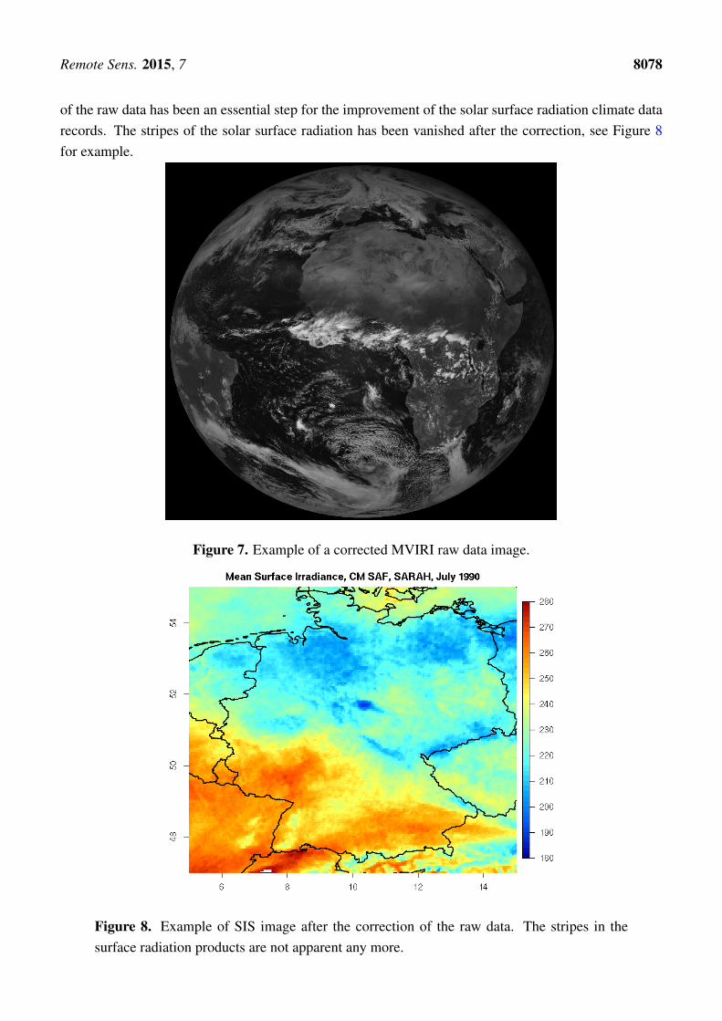
Remote Sens. 2015, 7 8078
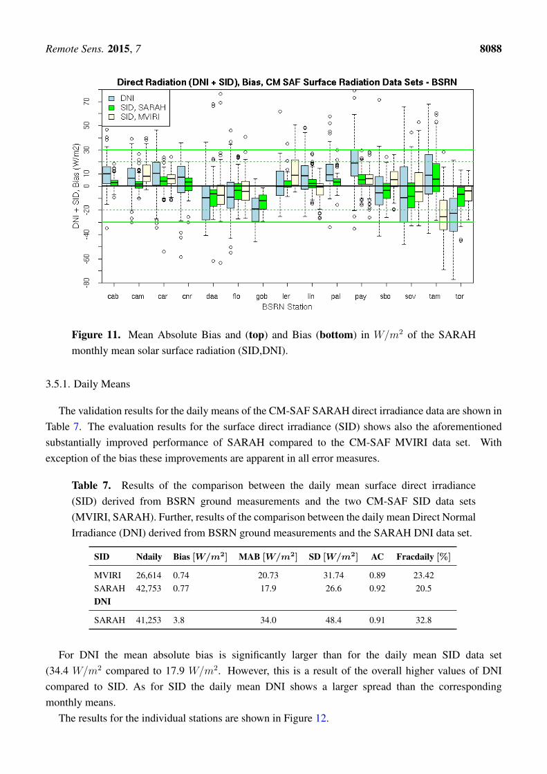
of the raw data has been an essential step for the improvement of the solar surface radiation climate datarecords. The stripes of the solar surface radiation has been vanished after the correction, see Figure 8for example.
Figure 7. Example of a corrected MVIRI raw data image.
Figure 8. Example of SIS image after the correction of the raw data. The stripes in thesurface radiation products are not apparent any more.

Remote Sens. 2015, 7 8079
The complete time series of the Meteosat satellites has been processed. The respective data coversthe period 1983–2013. Table 2 provides a list of the used satellite data sets.
Table 2. Major operational periods of the Meteosat satellites used for the generationof SARAH.
Satellite from to
MFG
Meteosat 2 16 August 1981 11 August 1988Meteosat 3 11 August 1988 19 June 1989Meteosat 4 19 June 1989 24 January 1990Meteosat 3 24 January 1990 19 April 1990Meteosat 4 19 April 1990 4 February 1994Meteosat 5 4 February 1994 13 February 1997Meteosat 6 13 February 1997 3 June 1998Meteosat 7 3 June 1998 31 December 2005
MSG
Meteosat 8 1 January 2006 April 2007Meteosat 9 1 May 2007 December 2012Meteosat 10 1 January 2013 December 2013
2.6.2. Aerosol
A monthly mean aerosol climatology has been generated by using the aerosol informationprovided by the European Centre for Medium Range Weather Forecast within the scope of the MACCproject–Monitoring Atmospheric Composition and Climate. The MACC data results from a dataassimilation system for global reactive gases, aerosols and greenhouse gases. It consists of a forwardmodel for aerosol composition and dynamics [44] and an data assimilation procedure [45]. It has recentlybeen used for the estimation of aerosol radiative forcing [46]. The MACC reanalysis data is generatedon a Gaussian T159 grid which corresponds to∼ 120 km spatial resolution. For the use within CM-SAFit has been regridded to a 0.5 × 0.5 degree regular latitude-longitude grid.
MACC has been evaluated to perform significantly better than the “Kinne” [47] GADS/OPAC [48,49]and HAC-v1 climatology [50], see [51] for details.
However, in a further study [52] it has been evaluated that a modification of the MACC AOD leads toan even better performance. The modification has been performed as described in Equation (12).
AODSARAH =
{AODMACC for AOD ≤ 0.160.16 + 0.5× AODMACC for AOD ≥ 0.16
(12)
Here, AODSARAH is the AOD used for the generation of the SARAH data set and AODMACC is theoriginal MACC AOD. The final climatology consists of monthly long term means on 0.5 × 0.5 degreelatitude-longitude grid. The respective AOD values are given for 550 nm. The pixel value is derived byspatial interpolation and assignment of the respective monthly mean.
Gueymard [53] and Nikitidou et al. [54] showed that the consideration of temporal variations ofaerosols as well as trends are important for the accurate retrieval of solar surface radiation, in particular

Remote Sens. 2015, 7 8080
for direct irradiance. Within this scope the use of a monthly aerosol climatology is a drawback. However,aerosol events as desert storms and biomass burning lead temporarily to an increase in CAL, which mightaccount partly for aerosol variations, please see [52] for further details.
2.6.3. Atmospheric Absorbers: Water Vapor and Ozone
Water vapor is an important atmospheric absorber, affecting solar surface radiation significantly.Integrated water vapor has been taken from from ERA-40 reanalysis [55,56] up to 1987 and from 1987
onwards from ERA-interim [57,58]. Monthly means, remapped to 0.25× 0.25 degree latitude-longitudegrid, has been used as input to SPECMAGIC. The pixel value is derived by spatial interpolation andassignment of the respective monthly mean.
Ozone is a strong absorber in the UV spectral range, but the absorption is quite weak within thebroadband spectrum, hence not of high relevance for the estimation the estimation of the solar surfaceirradiance. Thus, for ozone the climatological values from the standard atmosphere are used [59].Information about the other atmospheric gases (e.g., O2) and the total number density is taken fromthe US standard atmosphere [59] .
2.6.4. Surface Albedo
For the surface albedo the spectral albedo functions of 20 land-use types originating from the NASACERES/SARB Surface Properties Project [60,61], available at [62], has been used as basis. Each landuse type comes with a spectral albedo curve covering 0.2 to 4.0 micrometers. In addition to these curvesmeasured spectral curves provided by libRadtran have been used to account for the spectral albedo dataas far as possible. Please see [24,33] for further details. The diurnal variation of the spectral surfacealbedo is determined as a function of solar zenith angle, as given by [63]. The scene dependent solarzenith adjustment factors needed for this function are also taken from the NASA CERES/SARB SurfaceProperties Project.
The land-use types are fixed throughout the year, hence seasonal variation of the surface albedo arenot considered, but the surface albedo information is only used for the calculation of the clear skyirradiance. This induces uncertainties of about 1%–2% in regions with frequent variations of snowcover. Occasionally higher uncertainties might occur.
3. Validation of the SARAH CDRs
In this section the validation results are presented and discussed.
3.1. Reference Data for Validation
The validation of the new data sets for the surface incoming solar radiation (SIS) and the surfaceincoming direct solar radiation (SID,DNI) is primarily performed by comparison with high-qualityground based measurements from the Baseline Surface Radiation Network (BSRN) [64]. The BSRNstations used for the validation are listed in Table 3. They cover the period from 1992 onwards.

Remote Sens. 2015, 7 8081
Table 3. List of BSRN stations used for the validation.
Station Country CodeLatitude Longitude Elevation
Data Since[degN ] [degE] [m]
Cabauw Netherlands cab 51.97 4,93 0 1.12.2005Camborne UK cam 50.22 −5.32 88 1.1.2001Carpentras France car 44.05 5.03 100 1.8.1996Cener Spain cnr 42,82 −1.6 471 1.7.2009De Aar South Africa daa −30.67 23.99 1287 1.5.2000Florianopolis Brasil flo −27.53 −48.52 11 1.6.1994Gobabeb Namibia gob −23.56 15.04 407 15.5.2012Lerwick UK ler 60.13 −1.18 84 1.1.2001Lindenberg Germany lin 52.21 14.12 125 1.9.1994Palaiseu Cedec France pal 48.71 2.21 156 1.6.2003Payerne Switzerland pay 46.81 6.94 491 1.9.1992Sede Boger Israel sbo 30.9 34.78 500 1.1.2003Solar Village Saudi Arabia sov 24.91 46.41 650 1.8.1998Tamanrasset Algeria tam 22.78 5.51 1385 1.3.2000Toravere Estonia tor 58.25 26.46 70 1.1.1999
Only those stations that have an overlap of at least 12 months with the satellite data were used.This leads to 15 stations, which are located mainly in the Northern hemisphere, but they cover themain climatic regions and a substantial part (1992–2013) of the satellite time period. The effectivecloud albedo (CAL), as a pure satellite product, cannot be validated by comparison with ground basedmeasurements directly. However, the accuracy of CAL can be estimated by error propagation from theaccuracy of the surface radiation, see Section 3.6 for further details.
Furthermore, the discussion of the validation results accounts for the non-systematic error of theBSRN data of 5W/m2 for measurements of solar surface irradiance (global irradiance) [64]. The BSRNdata has been obtained from the BSRN archive at the Alfred Wegener Institute (AWI), Bremerhaven,Germany (www.bsrn.awi.de). In a first step the BSRN data has been quality controlled using the testsproposed by [65]. To ensure a high quality of the reference data set, only those BSRN measurementsthat pass the limit tests are considered in the calculation of the daily and monthly averages. To derivemonthly- and daily-averaged values from the surface measurements, the method M7 proposed by [66]was employed to reduce the impact of missing values. The uncertainty of the derived monthly means ison average ±8 W/m2 [28].
To assess the quality of the satellite data set with the BSRN surface observations, the difference in thespatial representativeness between these two observing systems needs also to be considered. Dependingon the local spatial distribution of surface radiation the impact can be in the range of 4W/m2 for monthlymean data [28] and even larger for daily mean surface radiation data. Due to its higher temporal andspatial variability it must be assumed that the level of uncertainty of the direct normal radiation (DNI)is larger than the level of uncertainty for solar surface irradiance (SIS). Further, circumsolar radiationcontributes to the direct irradiance. This contributes to an enhanced uncertainty of DNI due to reasonsrelated to different measurement geometries as well as differences relative to the definition of directirradiance in RTM or solar energy applications, please see [67] for further details.

Remote Sens. 2015, 7 8082
For a climate data record it is of interest to assess also the temporal stability with long-term referencemeasurements. BSRN measurements are not available before 1992, therefore data from the longer timeseries of the Global Energy and Balance Archive (GEBA) project has been used for this purpose. GEBAcontains monthly mean surface irradiance data sets from ground observations including stations reportingprior to 1983 [68]. The temporal homogeneity of the GEBA stations has been evaluated by [69]. About50 European stations have been found to be homogeneous over time. The data of these stations havebeen used to assess the temporal stability of the monthly mean SARAH SIS data set.
In addition to the validation with surface measurements, the quality of the CM-SAF SARAH dataset is evaluated against the quality of the first release of the CM-SAF surface radiation data based onobservation of the MVIRI instruments only, covering the period from 1983 to 2005 [25,36]. This dataset is referred to as CM-SAF MVIRI data set throughout of the paper. It has been widely used andevaluated by numerous users over the last years. (e.g., [29,30,69–71]).
3.2. Statistical Measures
The validation employs several statistical measures and scores to evaluate the quality of the solarsurface radiation data sets. Beside the commonly used bias and standard deviation, we also use the(mean) absolute difference (also referred to as Mean Absolute Bias) and the correlation of the anomaliesderived from the surface measurements and the CM-SAF data set. For each data set we further providethe number of months that exceed the target accuracy to characterize the quality of the data sets.
In the following, the applied quality measures are described. The definitions of the statistical measuresare taken from [72]. Thereby, the variable y describes the data set to be validated (e.g., SARAH) and odenotes the reference data set (i.e. BSRN). The individual time step is marked with k and n is the totalnumber of time steps.
Bias: The bias (or mean error) is the mean difference between the two considered datasets. It indicateswhether the data set on average over- or underestimates the reference data set.
Bias =1
n
n∑k=1
(yk − ok) = y − o (13)
Mean Absolute Bias (MAB): In contrast to the bias, the mean absolute bias (MAB) is the average ofthe absolute values of the differences between each member of the time series.
MAB =1
n
n∑k=1
|yk − ok| (14)
The MAB is also referred to as Mean Absolute Difference (MAD). The advantage of the MAB isthat there is no cancellation of positive and negative (bias) values.
Standard deviation (SD): The standard deviation SD is a measure for the spread around the meanvalue of the distribution formed by the differences between the generated and the referencedata set.
SD =
√√√√ 1
n− 1
n∑k=1
((yk − ok)− (y − o))2 (15)

Remote Sens. 2015, 7 8083
Anomaly correlation (AC): The anomaly correlation AC describes to which extend the anomaliesof the two considered time series correspond to each other without the influence of a possiblyexisting bias. The correlation of anomalies retrieved from satellite data and derived fromsurface measurements allows the estimation of the potential to determine anomalies fromsatellite observations.
AC =
∑nk=1 (yk − y) (ok − o)√∑n
k=1 (yk − y)2√∑n
k=1 (ok − o)2(16)
Here, for each station the mean annual cycle were derived separately from the satellite and surfacedata, respectively. The monthly/daily anomalies were then calculated using the correspondingmean annual cycle as the reference.
Fraction of time steps above the validation threshold (Frac): A measure for the uncertainty of thederived data set is the fraction of the time steps that are outside the requested thresholds Th.
Frac = 100
∑nk=1 fkn
with
fk = 1 if yk > Th
fk = 0 otherwise(17)
3.3. Validation Results—Comparison Method
The daily and monthly means of the SARAH data set are compared with the respective daily andmonthly means derived from the BSRN measurements. The means of the BSRN station have beenderived independently using the complete temporal resolution (minutes) of the BSRN measurements.The comparison results in a mean bias, mean absolute difference, anomaly correlation, standard deviationand fraction of months above a given limit for each individual station and for all stations together.
Daily and monthly mean of DNI are calculated by an arithmetic average. SIS and SID data areaveraged by application of an equation by Diekmann [73], which is preferable because of the largedependency on the solar zenith angle of SIS and SID, which makes the arithmetic averaging verysensitive to data gaps.
3.4. Validation Results—SIS
In this section the validation results of the Surface Incoming Solar Radiation, SIS are presented anddiscussed. The results of the validation of the monthly mean SARAH SIS data set are summarizedin Table 4. The bias and the MAB are with values of 1.27 and 5.46 W/m2 remarkably low. In totalabout 94% of the monthly mean values show an accuracy better than 10 W/m2, by consideration of anuncertainty of the surface measurement of 5 W/m2 [64] . The results show that the accuracy is closeto that of the ground measurements. The data set is also able to reproduce the anomalies of SIS quitewell, which is documented by the high correlation of the monthly SARAH SIS anomalies (0.92) withthe ground measurements . Also included in Table 4 are the corresponding statistical error measures ofthe CM-SAF MVIRI surface radiation data set [36]. It is clear that the quality of the new CM-SAF dataset SARAH is substantially improved compared to the previously released CM-SAF MVIRI data set.
An illustration of the bias and the MAB at each BSRN station is shown in Figure 9. The box-whiskerplots represent the range between the 25 and 75 percentiles (1st and 3rd quartile) by the colored boxes;

Remote Sens. 2015, 7 8084
the whiskers extend to 1.5 times the inter-quantile range or the maximum value, whichever is smaller.As already shown in Table 4, the new SARAH surface radiation data set has a substantially reduced biasand a lower MAB compared to the MVIRI CM-SAF surface radiation data set at each BSRN station.Particular improvements can be found at the BSRN stations Lerwick (ler), Carpentras (car), and SedeBoquer (sbo).
Figure 9. Mean Absolute Bias (top) and bias (bottom) in W/m2 of the SARAH monthlymean solar surface irradiance.
Table 4. Results of the comparison between the monthly mean surface solar irradiancederived from BSRN measurements and the two CM-SAF surface radiation data sets.
SIS Nmon Bias [W/m2] MAB [W/m2] SD [W/m2] AC Fracmon [%]
SARAH 1672 1.27 5.46 7.34 0.92 5.6MVIRI 878 4.24 7.76 8.23 0.89 10.71

Remote Sens. 2015, 7 8085
3.4.1. Daily Means
Table 5 provides the validation result for the daily means of the new SARAH SIS data set and theprevious CM-SAF MVIRI climate data record. As expected, the mean bias is almost identical to thevalue for the monthly means while the mean absolute bias for the daily means are about twice as highcompared to those for the monthly means. However, an increase of MAB values has to be expected asa result of an decreasing averaging period, due to the fact that satellite data are compared to groundmeasurements. The basis for the comparison are half hourly means of satellite data representing a3 × 5 km area with BSRN data representing point measurements. This reduces the comparability andincreases the deviation between the data, e.g., MAB, for short averaging periods. Still, the mean absolutebias of 12.1 W/m2 between daily mean SARAH SIS and BSRN is remarkable low. Further, nearly 90%of the daily means show better accuracy than 15W/m2. As for the monthly mean validation, the SARAHSIS data set shows improved performance for each quality measure compared to the CM-SAF MVIRISIS data set.
Table 5. Results of the comparison between the daily mean surface solar irradiance derivedfrom BSRN measurements and the two CM-SAF surface radiation data sets.
SIS Ndaily Bias [W/m2] MAB [W/m2] SD [W/m2] AC Fracdaily [%]
SARAH 48,413 1.12 12.1 17.9 0.95 11.3MVIRI 29,790 4.41 15.1 23.4 0.92 16.3
The bias and the MAB of the SIS daily mean from the SARAH data set for the individual BSRNstations are shown in Figure 10.
Figure 10. Cont.

Remote Sens. 2015, 7 8086
Figure 10. Mean Absolute Bias and (top) and Bias (bottom) in W/m2 of the SARAH dailymean solar surface irradiance.
3.5. Validation Results: SID and DNI
This section presents the validation results of the SARAH direct radiation data sets (SID and DNI)compared to the BSRN surface reference observations. DNI is derived by division of SID with the solarzenith angle (SZA), see Equation (11). This means that the physics (retrieval method) applied to deriveSID and DNI are identical. Table 6 shows the results of the validation of the surface direct radiation (SID)for the recent SARAH and the previous CM-SAF MVIRI data sets. The bias and the mean absolute biasare with 0.89 W/m2 and 8.2 W/m2 remarkably low for SID, showing the high accuracy of the data set.The MAB is thereby significantly lower than for the MVIRI data set. The substantial improvement ofSARAH SID relative to MVIRI SID is also apparent in the other validation measures.
Table 6. Results of the comparison between the monthly mean surface direct irradiance(SID) derived from BSRN ground measurements and the two CM-SAF SID data sets(MVIRI, SARAH). Further, results of the comparison between the monthly mean DirectNormal Irradiance (DNI) derived from BSRN ground measurements and the SARAH DNIdata set.
SID Nmon Bias [W/m2] MAB [W/m2] SD [W/m2] AC Fracmon [%]
MVIRI 805 0.89 11.0 15.7 0.83 15.4SARAH 1587 0.98 8.2 11.6 0.89 8.4
DNISARAH 1529 3.2 17.5 22.9 0.87 16.4

Remote Sens. 2015, 7 8087
For the solar energy community the direct normal irradiance is of high interest. Hence, the newSARAH data set offers the direct normal irradiance in addition to SIS and SID. DNI is not availablefrom the older CM-SAF MVIRI data set. A small bias of 3.2 W/m2 is found in the SARAH DNI dataset. The mean absolute bias is 17.5 W/m2. Considering the uncertainty of the surface measurement ofabout 10 W/m2, it can be expected that the accuracy of DNI is of about 10 W/m2, which is remarkablygood. The standard deviation and, thus, the spread is slightly larger for DNI than for SIS (22.9 W/m2
compared to 11.6 W/m2), which results simply from the fact that DNI exhibits on average higher valuesthan SID, due to the normalization with the cosine of solar zenith angle. This explains also that DNIshows larger values for Fracmon. The anomaly correlation shows a value of 0.87 and is almost identicalto the respective SARAH SID value.
The results for the individual BSRN stations are shown in Figure 11. Beside the SID results (SARAHand MVIRI) the figure shows also the absolute bias of the monthly means of DNI and of SID fromSARAH for each station. For most stations, the accuracy of SID from SARAH has improved comparedto the previous CM-SAF MVIRI data set.
Notably is the large negative offset in Toravere of about of about −27 W/m2 (Figure 11 bottom),which corresponds to a negative offset in SID of about 10 W/m2.
A reason for the relative large offset in Toravere could be an overestimation of clouds induces by theslant viewing geometry. For the same cloud scene the effective cloud albedo increases significantly forslant geometries as the effective cross section of the clouds observed from satellite increases. Further, forSID and DNI higher uncertainties are also expected in regions with high temporal and spatial variabilityin aerosol properties.
Figure 11. Cont.
Remote Sens. 2015, 7 8088
Figure 11. Mean Absolute Bias and (top) and Bias (bottom) in W/m2 of the SARAHmonthly mean solar surface radiation (SID,DNI).
3.5.1. Daily Means
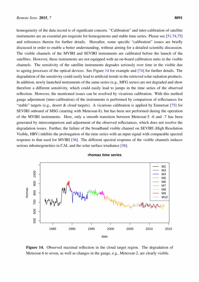
The validation results for the daily means of the CM-SAF SARAH direct irradiance data are shown inTable 7. The evaluation results for the surface direct irradiance (SID) shows also the aforementionedsubstantially improved performance of SARAH compared to the CM-SAF MVIRI data set. Withexception of the bias these improvements are apparent in all error measures.
Table 7. Results of the comparison between the daily mean surface direct irradiance(SID) derived from BSRN ground measurements and the two CM-SAF SID data sets(MVIRI, SARAH). Further, results of the comparison between the daily mean Direct NormalIrradiance (DNI) derived from BSRN ground measurements and the SARAH DNI data set.
SID Ndaily Bias [W/m2] MAB [W/m2] SD [W/m2] AC Fracdaily [%]
MVIRI 26,614 0.74 20.73 31.74 0.89 23.42SARAH 42,753 0.77 17.9 26.6 0.92 20.5DNI
SARAH 41,253 3.8 34.0 48.4 0.91 32.8
For DNI the mean absolute bias is significantly larger than for the daily mean SID data set(34.4 W/m2 compared to 17.9 W/m2. However, this is a result of the overall higher values of DNIcompared to SID. As for SID the daily mean DNI shows a larger spread than the correspondingmonthly means.
The results for the individual stations are shown in Figure 12.

Remote Sens. 2015, 7 8089
Figure 12. Mean Absolute Bias and (top) and bias (bottom) in W/m2 of the SARAH dailymean direct normal irradiance–DNI.
The daily means show the same features as the monthly mean direct radiation products. Relativelylarge mean absolute bias values are found at the predominantly sunny, cloud free (desert) stations ofGobabeb, Sede Boqer, Solar Village and Tamanrasset.
3.6. Validation Results: CAL
CAL is only observable from space. Thus, it can not be validated with ground based referencedata sets. However, its accuracy can be estimated by error propagation using the relation between SIS

Remote Sens. 2015, 7 8090
and CAL. The relation between the effective cloud albedo CAL and the solar irradiance is essentiallygiven by:
CAL = 1− SIS/SISclear (18)
Uncertainties in SIS are due to uncertainties in the effective cloud albedo and due to uncertaintiesin the clear sky irradiance. Here we assume a perfect clear sky irradiance (no errors), which relates alluncertainties in SIS to the effective cloud albedo and provides thus a worst case scenario for the CALaccuracy. The clear sky irradiance is, of course, not error free, hence the CAL errors are lower than theestimated values. Thus, based on Equation (18) the “worst case” accuracy of the effective cloud albedocan be derived as a function of the clear sky irradiance. Figure 13 shows the maximal error in the cloudindex, which would only be given for a mean absolute bias of zero in the clear sky irradiance. It isclear that this evaluation method is a workaround, but as aforementioned the effective cloud albedo is asatellite observable, and can thus not be “validated” with ground based reference data. However, as aresult of the low error in SIS it can be expected that the uncertainty in CAL is usually significantly belowof 0.1, with exception of bright surfaces (desert, snow) and slant viewing geometries where higher errorshave to be expected. Higher uncertainties in CAL affects also SIS, SID and DNI.
Figure 13. Maximal uncertainty of the monthly mean cloud albedo in dependency of theclear sky irradiance. The estimation of the CAL uncertainty is derived by error propagationbased on Equation 18. It depends therefore on the clear sky solar surface irradiance.
3.7. Homogeneity/Stability of CDRs
High accuracy (Bias, MAB) and precision (SD, Fracmon) are the main quality measures formonitoring of climate extremes and solar energy applications. However, for trend analysis the temporal
Remote Sens. 2015, 7 8091
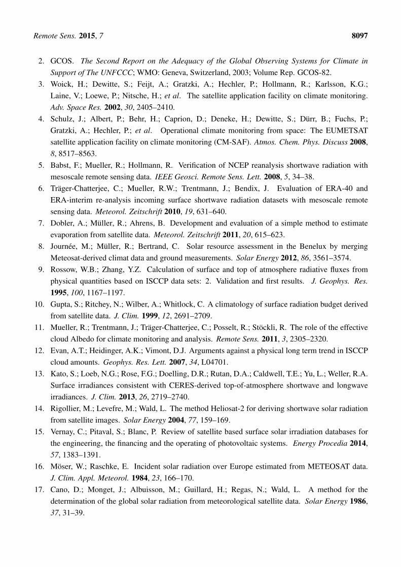
homogeneity of the data record is of significant concern. “Calibration” and inter-calibration of satelliteinstruments are an essential pre-requisite for homogeneous and stable time series. Please see [51,74,75]and references therein for further details. Hereafter, some specific “calibration” issues are brieflydiscussed in order to enable a better understanding, without aiming for a detailed scientific discussion.The visible channels of the MVIRI and SEVIRI instruments are calibrated before the launch of thesatellites. However, these instruments are not equipped with an on-board calibration units in the visiblechannels. The sensitivity of the satellite instruments degrades seriously over time in the visible dueto ageing processes of the optical devices. See Figure 14 for example and [74] for further details. Thedegradation of the sensitivity could easily lead to artificial trends in the retrieved solar radiation products.In addition, newly launched instruments of the same series (e.g., MFG series) are not degraded and showtherefore a different sensitivity, which could easily lead to jumps in the time series of the observedreflection. However, the mentioned issues can be resolved by vicarious calibration. With this methodgauge adjustment (inter-calibration) of the instruments is performed by comparison of reflectances for“stable” targets (e.g., desert & cloud targets). A vicarious calibration is applied by Eumetsat [75] forSEVIRI onboard of MSG (starting with Meteosat-8), but has been not performed during the operationof the MVIRI instruments. Here, only a smooth transition between Meteosat-5 -6 and -7 has beengenerated by intercomparison and adjustment of the observed reflectances, which does not resolve thedegradation issues. Further, the failure of the broadband visible channel on SEVIRI (High ResolutionVisible, HRV) inhibits the prolongation of the time series with an input signal with comparable spectralresponse to that used for MVIRI [36]. The different spectral response of the visible channels inducesserious inhomogeneities in CAL and the solar surface irradiance [36].
1985 1990 1995 2000 2005 2010 2015
500
600
700
800
900
1000
date
rhom
ax
rhomax time series
M2M3M4M5M6M7M8M9M10
Figure 14. Observed maximal reflection in the cloud target region. The degradation ofMeteosat-6 to seven, as well as changes in the gauge, e.g., Meteosat-2, are clearly visible.

Remote Sens. 2015, 7 8092
Summarizing, the change of satellite instruments of one series as well as the update to a newgeneration of satellite instruments can induce inhomogeneities in the retrieved effective cloud albedoand thus the solar surface irradiance. The generation of a homogeneous climate data record fromsatellite images in the visible is a quite challenging task. This might be one reason for the minor role ofremote sensing data in climate trend analysis, although that satellites are the only observational sourceof information over the oceans and many other regions of the world. Thus, analysis of the homogeneityof SARAH is an important issue.
A common method to assess the homogeneity of a climate data set is to analyze the anomaly timeseries for any obvious jumps. Changes in the mean state from one satellite to the other would be apparentas an increase or decrease in positive or negative anomalies. Figure 15 shows the Hovmoeller diagramof the monthly mean anomalies of SIS and DNI. The time covers the full period of the SARAH data setstarting with Meteosat 2 in 1983 until Meteosat 10 in 2013. No obvious artificial jumps or trends areapparent in the time series of the anomaly for the whole time period, indicating a good homogeneity ofthe SARAH data set.
Figure 15. Hovmoller diagrams of the monthly mean anomaly of SIS. and (bottom) DNI.
To evaluate and quantify the stability of the SARAH data set in more detail, references measurementsfrom the GEBA data base are used in addition to BSRN. While the BSRN observations follow a highquality standard and are considered as a GCOS reference observing network, the data in the GEBA database have a longer temporal coverage, which is important for the assessment of the temporal stability.To assess the temporal stability of the satellite-based data, the reference observations need to be stableover time as well. Selected European GEBA stations have been assessed with respect to their temporalstability and adjusted to ensure their homogeneity [69], only these stations are considered here.
Figure 16 shows the temporal evolution of the average bias between the monthly mean SARAH SISdata set and the measurements from the GEBA stations. Only stations with more than 95% availablemonthly means between 1983 and 2011 are considered to avoid artificial shifts in the mean time series

Remote Sens. 2015, 7 8093
due to changes in data availability. An optimal stability and match with the ground based stations wouldmean that no significant gradient in the linear regression is apparent. Any significant gradient indicatesa mismatch between the trends of satellite and ground based data.
Figure 16. Temporal evolution of the normalized differences between the CM-SAF data setand the GEBA data. The green line represents the zero line, the black and the blue straightlines represent the linear regression of the time series for the time periods 1983 to 2011 and1983 to 2005 (both for SARAH), respectively. A gradient of zero in the linear regressionwould mean a perfect match between trends in the satellite and ground based data. Alsogiven in the legend is the result of the analysis for MVIRI. However, the MVIRI trend isnot diagrammed.
A negative decadal gradient of the bias of −1.1 W/m2/decade is detected between satellite andground based data. This gradient is found to be statistically significant, but is rather small and mightbe in the range of the uncertainty of the ground measurements. This means that for trend analysisof the SARAH data set an uncertainty of about 1 W/m2/decade can be assumed for the time period1983–2013.
Figure 16 shows also the corresponding trend analysis for the time period 1983-2005 for the SARAHand the CM-SAF MVIRI solar surface radiation. (Note that the MVIRI trend is not diagrammed, butonly the numbers are given in the figure). While the bias of the MVIRI data set exhibits a significantnegative trend of −1.2 W/m2/dec compared to the GEBA surface observations the SARAH SIS dataset does not show a significant trend for the period 1983–2005. This is a remarkable improvement anddemonstrates the enhanced stability of the SARAH data set compared to the previous CM-SAF MVIRIsurface radiation data set. It is likely that the efforts concerning the raw data (Section 2.6) has been

Remote Sens. 2015, 7 8094
significantly contributed to this result. However, the differences in the SARAH trends for the period1983–2005 relative to 1983–2013 indicates a serious break induced by the transition from MFG to MSG,which is also visible in the development of the bias over time, see Figure 16. It is likely that this break isresulting from a sub-optimal generation of the artificial HRV channel. It is evident that an adjustment ofthe channel combination is needed.
Nevertheless, overall the homogeneity of SARAH is remarkably high, in particular when consideringthat ground measurements are not a-priory homogeneous but require homogenization tests as well. Inthis respect the SARAH data set is an important key for the supplementation of climate trend analysisbased on ground based measurements, in particular as many regions are not covered by well maintainedground based measurements.
Figure 17. Trend in the SARAH solar surface irradiance for the time periods 1983 to 2013.
Remote sensing based radiation products are the only observational sources that can provide trendsof surface radiation with high spatial resolution and large geographical coverage. Figure 17 shows thetrend for the full disk. It is evident that in many regions the trend is much higher than the expecteduncertainty of 1 W/m2/dec. The large spatial structures in the trends demonstrate the importance ofremote sensing radiation data for climate trend analysis. The large negative trends in the ITC regionmight indicate an enforcement and some latitudinal spreading of the Hadley circulation. This might beone driver for the positive trends in the sub-tropics and Central Europe. The significant negative trend

Remote Sens. 2015, 7 8095
close to the Antarctic might be one reason for the increase of the ice sheet there. Further trends and theiranalysis will be discussed in a forthcoming paper.
4. Conclusions
The CM-SAF SARAH data set and its retrieval method has been presented and discussed. It is the firsttime that the SPECMAGIC [24] eigenvector-hybrid LUT approach has been exploited for the retrievalof a CDR of broadband solar surface irradiance.
The satellite-derived SARAH climate data records of the surface incoming solar and direct normalradiation (SIS and DNI) have been validated by comparison with observations from 15 high qualityground-based stations of the BSRN network. For the solar surface irradiance (SIS) the bias of 1.3 W/m2
and mean absolute bias of 5.5 W/m2 are close to the uncertainty of the ground based measurements formonthly means, and hence, close to the optimal accuracy of 3–5 W/m2. For SID, the bias and MABare with 1 and 8 W/m2 remarkably good (3.1 and 17.5 W/m2 for DNI, respectively). By considerationof the uncertainty of the ground based measurements it can be assumed that the accuracy is better than8 W/m2 for SID and better than 12 W/m2 for DNI. However, for both SID and DNI there is room andneed for improvement of the accuracy.
The anomaly correlation show for all products very high values of about 0.9. The fraction of monthlyvalues that meets high accuracies is around 85%–95%. Thus, SARAH radiation products are well suitedfor climate monitoring and analysis of extremes.
Prior to 1992 no BSRN measurements are available, hence the data set could not be validated withBSRN ground based measurements for the period 1983–1992. However, there is no physical reasonwhy the accuracy of the climate data set should be significantly lower for this period. This argument is“proven” by comparison with GEBA measurements.
The evaluation of the CM-SAF SARAH solar surface irradiance with the old CM-SAF MVIRI surfaceradiation data set shows that the monthly and daily mean SARAH data have a higher quality than theprevious CM-SAF MVIRI surface radiation data set.
Visual inspection and correction of the MVIRI raw data base has been performed. It is likely thatthis, together with an improved retrieval procedure have significantly contributed to the good SARAHvalidation results.
Special care has been taken to improve the homogeneity of the CDR. The stability of the SARAHSIS data set has been validated against European surface measurements (GEBA). A statisticallysignificant negative trend in the bias of −1.1 W/m2/dec was found between SARAH and ground basedmeasurements for the period 1983–2013. It can be assumed that trend analysis based on SARAH hasan uncertainty of about 1 W/m2/dec. However, for the period covered by the CM-SAF MVIRI dataset (1983–2005) no significant trend in the bias has been found in the SARAH data set. In contrast,the CM-SAF MVIRI data set shows a significant trend in the bias of −1.2 W/m2/dec for the sameperiod (1983–2005). This demonstrates that the homogeneity of SARAH has significantly improvedcompared to the CM-SAF MVIRI data set. Further, it clearly indicates that the transition from MVIRI toSEVIRI induces a slight inhomogeneity in the SARAH data set. Nevertheless, overall, it is shown thatthe SARAH data set can be expected to be well suited for climate trend analysis.

Remote Sens. 2015, 7 8096
The uncertainty of the effective cloud albedo is in general better than 10%. The validationresults show that the SARAH radiation records are in general well suited for climate monitoringand analysis.
Acknowledgments
This work is partly funded by EUMETSAT within the SAF framework. We thank the European taxpayers, as the funding is originally given by them. The authors thank the operations team of CM-SAFfor their support.
Author Contributions
Uwe Pfeifroth and Richard Müller generated the SARAH data set. Jörg Trentmann did thevalidation of SARAH. Christine Träger-Chatterjee, Uwe Pfeifroth and Roswitha Cremer worked on theimprovement of the atmospheric input data. Richard Müller developed the SPECMAGIC algorithm andwrote large parts of the manuscript. All authors contributed to the writing and editing of the manuscript.
Conflicts of Interest
The authors declare no conflict of interest.
Glossary–List of Acronyms in Alphabetical Order
AOD: Aerosol Optical DepthCAL: Effective Cloud AlbedoDNI: Direct Normal Irradiancek: Clear sky indexLUT: Look-up tableMACC: Monitoring Atmospheric Composition and ClimateMFG: Meteosat First GenerationMVIRI : Meteosat Visible-InfraRed ImagerMSG: Meteosat Second GenerationsRTM: Radiative Transfer ModelSEVIRI: Spinning Enhanced Visible and Infrared ImagerSID: Surface Direct Irradiance (beam)SIS: Solar Surface IrradianceSZA : Sun Zenith AngleSSA: Single Scattering Albedo
References
1. Schmetz, J.; Pili Tjemkes, P.S.; Just, D.; Kerkmann, J.; Rota, S.; Ratier, A. An introduction toMeteosat Second Generation (MSG). Bull. Am. Met. Soc. 2002, 83, 977–992.
Remote Sens. 2015, 7 8097
2. GCOS. The Second Report on the Adequacy of the Global Observing Systems for Climate inSupport of The UNFCCC; WMO: Geneva, Switzerland, 2003; Volume Rep. GCOS-82.
3. Woick, H.; Dewitte, S.; Feijt, A.; Gratzki, A.; Hechler, P.; Hollmann, R.; Karlsson, K.G.;Laine, V.; Loewe, P.; Nitsche, H.; et al. The satellite application facility on climate monitoring.Adv. Space Res. 2002, 30, 2405–2410.
4. Schulz, J.; Albert, P.; Behr, H.; Caprion, D.; Deneke, H.; Dewitte, S.; Dürr, B.; Fuchs, P.;Gratzki, A.; Hechler, P.; et al. Operational climate monitoring from space: The EUMETSATsatellite application facility on climate monitoring (CM-SAF). Atmos. Chem. Phys. Discuss 2008,8, 8517–8563.
5. Babst, F.; Mueller, R.; Hollmann, R. Verification of NCEP reanalysis shortwave radiation withmesoscale remote sensing data. IEEE Geosci. Remote Sens. Lett. 2008, 5, 34–38.
6. Träger-Chatterjee, C.; Mueller, R.W.; Trentmann, J.; Bendix, J. Evaluation of ERA-40 andERA-interim re-analysis incoming surface shortwave radiation datasets with mesoscale remotesensing data. Meteorol. Zeitschrift 2010, 19, 631–640.
7. Dobler, A.; Müller, R.; Ahrens, B. Development and evaluation of a simple method to estimateevaporation from satellite data. Meteorol. Zeitschrift 2011, 20, 615–623.
8. Journée, M.; Müller, R.; Bertrand, C. Solar resource assessment in the Benelux by mergingMeteosat-derived climat data and ground measurements. Solar Energy 2012, 86, 3561–3574.
9. Rossow, W.B.; Zhang, Y.Z. Calculation of surface and top of atmosphere radiative fluxes fromphysical quantities based on ISCCP data sets: 2. Validation and first results. J. Geophys. Res.1995, 100, 1167–1197.
10. Gupta, S.; Ritchey, N.; Wilber, A.; Whitlock, C. A climatology of surface radiation budget derivedfrom satellite data. J. Clim. 1999, 12, 2691–2709.
11. Mueller, R.; Trentmann, J.; Träger-Chatterjee, C.; Posselt, R.; Stöckli, R. The role of the effectivecloud Albedo for climate monitoring and analysis. Remote Sens. 2011, 3, 2305–2320.
12. Evan, A.T.; Heidinger, A.K.; Vimont, D.J. Arguments against a physical long term trend in ISCCPcloud amounts. Geophys. Res. Lett. 2007, 34, L04701.
13. Kato, S.; Loeb, N.G.; Rose, F.G.; Doelling, D.R.; Rutan, D.A.; Caldwell, T.E.; Yu, L.; Weller, R.A.Surface irradiances consistent with CERES-derived top-of-atmosphere shortwave and longwaveirradiances. J. Clim. 2013, 26, 2719–2740.
14. Rigollier, M.; Levefre, M.; Wald, L. The method Heliosat-2 for deriving shortwave solar radiationfrom satellite images. Solar Energy 2004, 77, 159–169.
15. Vernay, C.; Pitaval, S.; Blanc, P. Review of satellite based surface solar irradiation databases forthe engineering, the financing and the operating of photovoltaic systems. Energy Procedia 2014,57, 1383–1391.
16. Möser, W.; Raschke, E. Incident solar radiation over Europe estimated from METEOSAT data.J. Clim. Appl. Meteorol. 1984, 23, 166–170.
17. Cano, D.; Monget, J.; Albuisson, M.; Guillard, H.; Regas, N.; Wald, L. A method for thedetermination of the global solar radiation from meteorological satellite data. Solar Energy 1986,37, 31–39.

Remote Sens. 2015, 7 8098
18. Bishop, J.; Rossow, W. Spatial and temporal variability of global surface solar irradiance.J. Geophys. Res. 1991, 96, 839–858.
19. Pinker, R.; Laszlo, I. Modelling surface solar irradiance for satellite applications on a global scale.J. Appl. Meteorol. 1992, 31, 166–170.
20. Darnell, W.; Staylor, W.; Gupta, S.; Ritchey, N.; Wilber, A. Seasonal variation of surface radiationbudget derived from ISCCP-C1 data. J. Geophys. Res. 1992, 97, 15741–15760.
21. Deneke, H.; Feijt, A. Estimation surface solar irradiance from METEOSAT SEVIRI-derived cloudproperties. Remote Sens. Environ. 2008, 112, 3131–3141.
22. Mueller, R.; Matsoukas, C.; Gratzki, A.; Hollmann, R.; Behr, H. The CM-SAF operationalscheme for the satellite based retrieval of solar surface irradiance–A LUT based eigenvector hybridapproach. Remote Sens. Environ. 2009, 113, 1012–1022.
23. Perez, R.; Ineichen, P.; Moore, K.; Kmiecik, M.; George, R.; Vignola, F. A new operational modelfor satellite-derived irradiances: description and validation. Solar Energy 2002, 73 , 307–317.
24. Mueller, R.; Behrendt, T.; Hammer, A.; Kemper, A. A new algorithm for the satellite-based retrievalof solar surface irradiance in spectral bands. Remote Sens. 2012, 4, 622–647.
25. Posselt, R.; Mueller, R.; Stöckli, R.; Trentmann, J. Remote sensing of solar surface radiation forclimate monitoring–The CM-SAF retrieval in international comparison. Remote Sens. Environ.2011, 118, 186–198.
26. DOI of CM-SAF MVIRI data set: 10.5676/EUM_SAF_CM/RAD_MVIRI/V001, 2011. Availableonline: http://dx.doi.org/10.5676/EUM_SAF_CM/RAD_MVIRI/V001 (accessed on 17 June2015).
27. Amillo, A.; Huld, T.; Müller, R. A new database of global and direct solar radiation using theeastern meteosat satellite. Remote Sens. 2014, 6, 8165–8189.
28. Hakuba, M.Z.; Folini, D.; Sanchez-Lorenzo, A.; Wild, M. Spatial representativeness ofground-based solar radiation measurements. J. Geophys. Res. 2013, 118, 8585–8597.
29. Hagemann, S.; Loew, A.; Andersson, A. Combined evaluation of MPI-ESM land surface water andenergy fluxes. J. Adv. Model. Earth Syst. 2013, 5, 259–286.
30. Huld, T.; Müller, R.; Gambardella, A. A new solar radiation database for estimating PVperformance in Europe and Africa. Solar Energy 2012, 86, 1803–1815.
31. Ohmura, A.; Dutton, E.G.; Forgan, B.; Fröhlich, C.; Gilgen, H.; Hegner, H.; Heimo, A.;Konig-Langlo, G.; McArthur, B.; Müller, G.; et al. Baseline Surface Radiation Network(BSRN/WCRP): New precision radiometry for climate research. Bull. Am. Meteorol. Soc. 1998,79, 2115–2136.
32. Hammer, A.; Heinemann, D.; Hoyer, C.; Kuhlemann, R.; Lorenz, E.; Mueller, R.; Beyer, H.Solar energy assessment using remote sensing technologies. Remote Sens. Environ. 2003,86, 423–432.
33. Mayer, B.; Kylling, A. Technical note: The libRadtran software package for radiative transfercalculationsdescription and examples of use. Atmos. Chem. Phys. 2005, 5, 1855–1877.
34. Stammes, K.; Tsay, S.; Wiscombe, W.; Jayaweera, K. Numerically stable algorithm fordiscrete-ordinate-method radiative transfer in multiple scattering and emitting layered media. Appl.Opt. 1988, 27, 2502–2509.

Remote Sens. 2015, 7 8099
35. Kato, S.; Ackerman, T.; Mather, J.; Clothiaux, E. The k-distribution method and correlated-kapproximation for a short-wave radiative transfer. J. Quant. Spectrosc. Radiat. Transfer 1999,62, 109–121.
36. Posselt, R.; Mueller, R.; Stöckli, R.; Trentmann, J. Spatial and temporal homogeneity of solarsurface irradiance across satellite generations. Remote Sens. 2011, 3, 1029–1046.
37. Mueller, R.; Dagestad, K.; Ineichen, P.; Schroedter-Homscheidt, M.; Cros, S.; Dumortier, D.;Kuhlemann, R.; Olseth, J.; Piernavieja, G.; Resie, C.; et al. Rethinking satellite based solarirradiance modelling. The SOLIS clear-sky module. Remote Sens. Environ. 2004, 91, 160–174.
38. Shettle, P.; Fenn, R.W. Models of the atmospheric aerosols and their optical properties. InProceedings of the AGARD Conference Proceedings No. 183, Optical Propagation in theAtmosphere, Symposium, Lyngby, Denmark, 27–31 October 1975.
39. Shetlle, E. Models of aerosols, clouds and precipitation for atmospheric propagation studies. InProceedings of the AGARD Conference Proceedings No. 454, Atmospheric propagation in theUV, Visible, IR and mm-Region and Related System Aspects, Electromagnetive Wave PropagationPanel Specialist Meeting, Copenhagen, Denmark, 9–13 October 1989.
40. Skartveit, A.; Olseth, J.; Tuft, M. An hourly diffuse fraction model with correction for variabilityand surface albedo. Solar Energy 1998, 63, 173–183.
41. EUMETSAT. The METEOSAT system. In Technical Report Revision 4; EUMETSAT: Darmstadt,Germany, 2000.
42. Cros, S.; Albuisson, M.; Wald, L. Simulating Meteosat-7 broadband radiances using two visiblechannels of Meteosat-8. Solar Energy 2006, 80, 361–367.
43. Posselt, R.; Mueller, R.; Trentmann, J.; Stockli, R.; Liniger, M. A surface radiation climatologyacross two Meteosat satellite generations. Remote Sens. Environ. 2014, 142, 103–110.
44. Morcrette, J.J.; Boucher, O.; Jones, L.; Salmond, D.; Bechtold, P.; Beljaars, A.; Benedetti, A.;Bonet, A.; Kaiser, J.W.; Razinger, M.; et al. Aerosol analysis and forecast in the European Centrefor Medium-Range Weather Forecasts Integrated Forecast System: Forward modeling. J. Geophys.Res. 2009, 114, doi:10.1029/2008JD011235
45. Benedetti, A.; Morcrette, J.J.; Boucher, O.; Dethof, A.; Engelen, R.; Fisher, M.; Flentje, H.;Huneeus, N.; Jones, L.; Kaiser, J.; et al. Aerosol analysis and forecast in the European Centrefor medium-range weather forecasts integrated forecast system: 2. Data assimilation. J. Geophys.Res. 2009, 114, doi:10.1029/2008JD011115.
46. Bellouin, N.; Quaas, J.; Morcrette, J.J.; Boucher, O. Estimates of aerosol radiative forcing from theMACC re-analysis. Atmos. Chem. Phys. 2013, 13, 2045–2062.
47. Kinne, S.; Schulz, M.; Textor, C.; Guibert, S.; Balkanski, Y.; Bauer, S.E.; Berntsen, T.;Berglen, T.F.; Boucher, O.; Chin, M.; et al. An AeroCom initial assessment-optical propertiesin aerosol component modules of global models. Atmos. Chem. Phys. 2006, 6, 1815–1834.
48. Hess, M.; Koepke, P.; Schult, I. Optical properties of aerosols and clouds: The software packageOPAC. Bull. Am. Meteorol. Soc. 1998, 79, 831–844.
49. Koepke, P.; Hess, M.; Schult, I.; Shettle, E. Global Aerosol Data Set; Technical Report No. 243;Max Planck Institut für Meteorologie: Hamburg, Germany, 1997.
Remote Sens. 2015, 7 8100
50. Kinne, S.; O’Donnel, D.; Stier, P.; Kloster, S.; Zhang, K.; Schmidt, H.; Rast, S.; Giorgetta, M.;Eck, T.F.; Stevens, B. MAC-v1: A new global aerosol climatology for climate studies. J. Adv.Model. Earth Syst. 2013, 5, 707–740.
51. Mueller, R.; Tráger-Chatterjee, C. Brief accuracy assessment of aerosol climatologies for theretrieval of solar surface radiation. Atmosphere 2014, 5, 9699–9729.
52. Müller, R.; Pfeifroth, U.; Träger-Chatterjee, C. Towards optimal aerosol information for solarsurface radiation retrieval using Heliosat. Atmosphere 2015, in press.
53. Gueymard, C.A. Temporal variability in direct and global irradiance at various time scales asaffected by aerosols. Solar Energy 2012, 86, 3544–3553.
54. Nikitidou, E.; Kazantzidis, A.; Salamalikis, V. The aerosol effect on direct normal irradiance inEurope under clear skies. Renew. Energ. 2014, 68, 475–484.
55. Uppala, S.; Kållberg, P.; Simmons, A.; Andreae, U.; da Costa Becthold, V.; Firino, M.; Gibson, J.;Haseler, J.; Hernandez, A.; Kelly, G.; et al. The ERA-40 re-analysis. Q. J. R. Meteorol. Soc. 2005,131, 2961–3012.
56. Betts, A.K.; Ball, J.H.; Bosilovich, M.; Viterbo, P.; Zhang, Y.; Rossow, W.B. Intercomparisonof water and energy budgets for five Mississippi subbasins between ECMWF re-analysis(ERA-40) and NASA Data Assimilation Office fvGCM for 1990–1999. J. Geophys. Res. 2003,108, doi:10.1029/2002JD003127.
57. Dee, D.P.; Uppala, S. Variational bias correction of satellite radiance data in the ERA-interimreanalyis. Q. J. R. Meteorol. Soc. 2009, 135, 1830–1841.
58. Dee, D.P.; Uppala, S.M.; Simmons, A.J.; Berrisford, P.; Poli, P.; Kobayashi, S.; Andrae, U.;Balmaseda, M.A.; Balsamo, G.; Bauer, P.; et al. The ERA-Interim reanalysis: configurationand performance of the data assimilation system. Q. J. R. Meteorol. Soc. 2011, 137, 553–597.
59. Krämer, M.; Müller, R.; Bovensmann, H.; Burrows, J.; Brinkmann, J.; Röth, E.; Grooß, J.U.;Müller, R.; Woyke, T.; Ruhnke, R.; et al. Intercomparison of stratospheric chemistry models underpolar vortex conditions. J. Atmos. Chem. 2003, 45, 51–77.
60. Loveland, T.; Belward. The IGBP-DIS global 1 km land cover data set, DISCover first results. Int.J. Remote Sens. 1997, 18, 3289–3295.
61. Brown, J.F.; Loveland, T.; Merchant, J.W.; Reed, B.C.; Ohlen, D.O. Using multi-source data inglobal land-cover characterization: Concepts, requirements, and methods. Photogramm. Eng.Remote Sens. 1993, 59, 977–987.
62. CERES/SARB SAL. Available online: http://mynasadata.larc.nasa.gov/ceres-surface-type-data(accessed on 17 June 2015).
63. Dickinson, R.E. Land surface processes and climate–Surface albedos and energy balance. Adv.Geophys. 1983, 25, 305–353.
64. Ohmura, A.; Dutton, E.; Forgan, B.; Fröhlich, C.; Hegner, H.; Heimo, A.;König-Langlo, G.; Mc Arthur, B.; Müller, G.; Philipopon, R.; et al. Baseline SurfaceRadiation Network (BSRN/WCRP): New precision radiometry for climate research. Bull. Am.Met. Soc. 1998, 79, 2115–2136.
65. Long, C.N.; Shi, Y. An automated quality assessment and control algorithm for surface radiationmeasurements. Open Atmos. Sci. J. 2008, 2, 23–37.

Remote Sens. 2015, 7 8101
66. Roesch, A.; Wild, M.; Ohmura, A.; Dutton, E.G.; Long, C.N.; Zhang, T. Assessment of BSRNradiation records for the computation of monthly means. Measur. Techn. Discuss. 2010, 3,339–354.
67. Blanc, P.; Espinar, B.; Geuder, N.; Meyer, R.; Pitz-Paal, R.; Reinhardt, B.; Renne, D.; Sengupta,M.; Wald, L.; Wilbert, S. Direct normal irradiance related definitions and applications: Thecircumsolar issue. Solar Energy 2014, 110, 561–577.
68. Gilgen, H.; Roesch, A.; Wild, M.; Ohmura, A. Decadal changes in shortwave irradiance atthe surface in the period from 1960 to 2000 estimated from global energy balance archive data.J. Geophys. Res., 2009, 114, doi:10.1029/2008JD011383.
69. Sanchez-Lorenzo, A.; Wild, M.; Trentmann, J. Validation and stability assessment of the monthlymean CM SAF surface solar radiation dataset over Europe against a homogenized surface dataset(1983–2005). Remote Sens. Environ. 2013, 134, 355–366.
70. Bojanowski, J.S.; Vrieling, A.; Skidmore, A.K. A comparison of data sources for creating along-term time series of daily gridded solar radiation for Europe. Solar Energy 2014, 99, 152–171.
71. Operations Reports of the CM-SAF. Available online: http://www.cmsaf.eu (assessed on 1 June2015).
72. Wilks, D.S. Statistical Methods in the Atmospheric Sciences, 2nd ed.; International GeophysicsSeries, Vol 59, Academic Press: New York, NY, USA, 2006, ISBN-13: 978-0127519654.
73. Diekmann, F.J.; Happ, S.; Rieland, M.; Benesch, W.; Czeplak, G.; Kasten, F. An operationalestimate of global solar irradiance at ground level from METEOSAT data: Results from 1985 to1987. Met. Rdsch. 1988, 41, 65–79.
74. Decoster, I.; Clerbaux, N.; Baudrez, E.; Dewitte, S.; Ipe, A.; Nevens, S.; Blazquez, A.V.;Cornelis, J. Spectral aging model applied to meteosat first generation visible band. Remote Sens.2014, 6, 2534–2571.
75. Govaerts, Y.; Clerici, M.; Clerbaux, N. Operational calibration of the meteosat radiometer VISband. IEEE Trans. Geosci. Remote Sens. 2004, 42, 1900–1914.
c© 2015 by the authors; licensee MDPI, Basel, Switzerland. This article is an open access articledistributed under the terms and conditions of the Creative Commons Attribution license(http://creativecommons.org/licenses/by/4.0/).