Remittances and Poverty in Ghana1

Kwabena Gyimah-BrempongDepartment of Economics

University of South Florida4202 East Fowler Avenue

Tampa, FL 33620email: kgyimah@coba.usf.edu

Tel: (813) 974 6520

and

Elizabeth AsieduDepartment of Economics

University of KansasLawrence, KS 66045email: asiedu@ku.edu

September 28, 2009

1Paper to be presented at the 4th African Economic Conference (AEC), Addis Ababa, Ethiopia, November2009. David Roodman suggested and provided the codes for the cmp program. We thank David Klinowskifor outstanding research assistance. Any remaining errors are, of course, our own.

Abstract

This paper investigates the effects of international remittances on poverty incidence and severityin Ghana. Using both cross section data from Ghana Living Standards Survey wave 5 (GLSS5)and pseudo-panel data constructed from GLSS3-GLSS5 and a GMM pseudo-panel estimator, wefind that international remittances decreases the probability of a family being poor or chronicallypoor. The effect of international remittances in reducing poverty is far higher than the effect ofdomestic remittances in reducing poverty. We also find that remittances increases the number ofchildren in a family that attend school, suggesting that international remittances increase humancapital formation. We interpret this to mean that international remittances also decreases povertyin the long run. Our results are robust to the measurement of “poverty”, sample, and estimationmethodology. Our results have important policy implications.

KEY WORDS: REMITTANCES, INTERNATIONAL, INTERNAL, GHANA, POVERTYIMPACTS CROSS-SECTION, PSEUDO-PANEL, GMM ESTIMATION

JEL: O, O1, O24, O54, F35, F43

1 Introduction

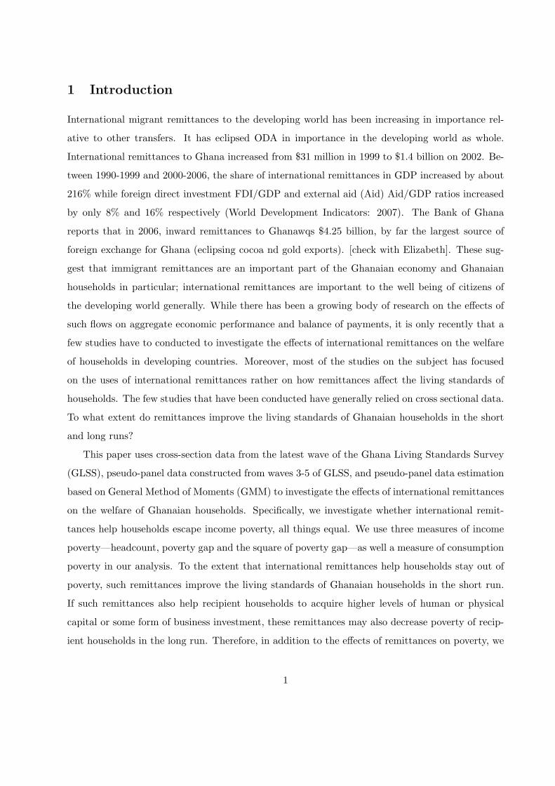
International migrant remittances to the developing world has been increasing in importance rel-

ative to other transfers. It has eclipsed ODA in importance in the developing world as whole.

International remittances to Ghana increased from $31 million in 1999 to $1.4 billion on 2002. Be-

tween 1990-1999 and 2000-2006, the share of international remittances in GDP increased by about

216% while foreign direct investment FDI/GDP and external aid (Aid) Aid/GDP ratios increased

by only 8% and 16% respectively (World Development Indicators: 2007). The Bank of Ghana

reports that in 2006, inward remittances to Ghanawqs $4.25 billion, by far the largest source of

foreign exchange for Ghana (eclipsing cocoa nd gold exports). [check with Elizabeth]. These sug-

gest that immigrant remittances are an important part of the Ghanaian economy and Ghanaian

households in particular; international remittances are important to the well being of citizens of

the developing world generally. While there has been a growing body of research on the effects of

such flows on aggregate economic performance and balance of payments, it is only recently that a

few studies have to conducted to investigate the effects of international remittances on the welfare

of households in developing countries. Moreover, most of the studies on the subject has focused

on the uses of international remittances rather on how remittances affect the living standards of

households. The few studies that have been conducted have generally relied on cross sectional data.

To what extent do remittances improve the living standards of Ghanaian households in the short

and long runs?

This paper uses cross-section data from the latest wave of the Ghana Living Standards Survey

(GLSS), pseudo-panel data constructed from waves 3-5 of GLSS, and pseudo-panel data estimation

based on General Method of Moments (GMM) to investigate the effects of international remittances

on the welfare of Ghanaian households. Specifically, we investigate whether international remit-

tances help households escape income poverty, all things equal. We use three measures of income

poverty—headcount, poverty gap and the square of poverty gap—as well a measure of consumption

poverty in our analysis. To the extent that international remittances help households stay out of

poverty, such remittances improve the living standards of Ghanaian households in the short run.

If such remittances also help recipient households to acquire higher levels of human or physical

capital or some form of business investment, these remittances may also decrease poverty of recip-

ient households in the long run. Therefore, in addition to the effects of remittances on poverty, we

1

also investigate the effects of remittances on human capital formation at the household level. We

measure human capital formation as the proportion of children in a household attending primary

or completing school and the proportion of children attending secondary school in the household.

Investigating the effects of international remittances on the welfare of households of sending

countries is of interest for a number of reasons. Among them, it is often argued that sending

countries lose to the receiving countries when their young and brightest, often educated at public

expense, emigrate to the latter countries that happen to be the developed countries. If remittances

improves living standards of sending countries, then such remittances may offset some of the cost to

the sending countries. Azam and Gubert (2006) argue that remittances must be seen as a contingent

flow from a joint family decision to send its young ones abroad in exchange for financial flows from

the emigrant to smoothen the family’s consumption. If that is the case, investigating remittances on

poverty will help shed light to what extent these flows fulfill the implicit contracts. Third, this study

shed some light not only on how remittances affect the poverty status of households in the short

run, but also how it determines poverty status in the long run through human capital formation.

Finally, investigating whether the gender of the recipient household head makes a difference in the

effect of remittances has important policy implication for household welfare and human capital

development.

Our paper makes important contributions to the literature on the relationship between remit-

tances and poverty in Less Developed Countries (LDCs). This paper uses both a cross section

and pseudo-panel data constructed from the last three waves of GLSS to investigate the effect of

remittances on poverty thus allowing us to compare the statics of poverty with possible dynamics

of the relationship. We also use several measures of poverty that makes it possible for us to in-

vestigate the robustness of the effects of remittances on different measures of poverty. Third, we

estimate the probability of being absolute poor or falling into relative poverty hence we use both

probit as well as ordered probit estimation methods. Fourth, we use the latest GMM pseudo-panel

data estimation methodology that provides consistent efficient estimates even in the presence of

individual and cohort fixed effects. Finally, our estimation methods and data sets allows us to

investigate the robustness of our results to the measurement of poverty as well as the estimation

method used.

Our results can briefly be summarized as follows: We find that international remittances reduces

the probability that a household will be poor either in the extreme sense or relative sense. This

2

results is robust to the measurement of poverty we use and the sample data—cross section or

pseudo-panel—we use. We also find that there is a gender effect on the remittances having an

effect on poverty incidence. We also find that the receipt of international remittances increases

the number of children who attend primary and secondary school. These results indicate that

international remittances have significant and positive effect on the education of children, hence

long-run poverty reduction in Ghana.

The rest of the paper is organized as follows. Section 2 reviews the literature on the effects of

remittances on poverty and consumption in Less Developed Countries (LDCs) generally and Africa

in particular. Section 3 presents the equation we estimate and discusses the estimation method

followed by a discussion the data and the construction of the pseudo-panel in section 4. Section 5

presents and discusses the results while section 6 concludes the paper.

2 Literature Review

Interest in the effects of international remittances on economic outcomes and household welfare

in LDCs has been on the increase in recent years. Although most of the empirical work has been

done for Latin American and Asian countries, a few studies have been done using African data.

We review some of the studies that are relevant for our paper in this section.

Adams (2004, 2006) uses survey data for Guatemala and Ghana to investigate the effects of

remittances from domestic and international migrants on poverty and income distribution. Using

a methodology that estimates what household expenditures would have been had the households

included the migrant, he finds that remittances reduce poverty but has no effect on income dis-

tribution in Guatemala and Ghana. The degree to which remittances impact poverty depends on

how one measures poverty. Guzman et al (2006) uses the GLSS4 data and an intra-household

bargaining framework to investigate the impact of gender of remittance recipients and senders on

the patterns of expenditures. They find that female-headed household that receive remittances

(withing Ghana and internationally) spend more on education, health, housing, and durable con-

sumer goods compared to female household heads who do not receive remittances or their male

counterparts.

Litchfield and Waddington (2003) uses GLSS3 and GLSS4 to investigate migration patterns

and the effects of migration of household welfare. They conclude that migration generally im-

3

prove the welfare of households as measured by probability of being poor, household expenditures,

and primary school enrollment of children in households. Our paper is similar to Litchfield and

Waddington’s except that we use pseudo-panel data estimation method to improve efficiency while

they limit themselves to cross section analysis. Glewe (1991) uses data from the Cote d’Ivoire

Living Standards Survey (CLSS) to investigate the determinants of welfare in Cote d’Ivoire and

finds that education, asset ownership (including farm equipment and land in rural areas, savings

and sector of employment are significant determinants of welfare.

Quartey and Blankson (2004) and Quartey (2006) use GLSS3-GLSS4 data and pseudo-panel

data estimation method to investigate the effects of remittances on income smoothing in Ghana.

They conclude that all things equal, remittances have been a source of income smoothing for Ghana-

ian especially during periods of macroeconomic instability. They estimated a random effects model.

However, as Inoue (2008) argues, both RE and FE are inconsistent in the presence of individual

or cohort fixed effects. Mukherjee and Benson (2003) investigates the determinants of poverty

in Malawi and finds education, age profile of household head, the composition of the household,

industry of employment, ownership of productive capital, as well as community characteristics are

important determinants of poverty. At the macro level, Gupta, Pattillo and Wagh (2007) uses panel

data to investigate the impact of remittances on poverty and financial development in Sub-Saharan

Africa and find that international remittances significantly reduces poverty and improves financial

development in Sub-Saharan Africa, all things equal.

Azam and Gubert (2006) investigates the effects of remittances on household in the Senegal

Valley in Mali and Senegal. They develop a model in which migration and remittances are joint

strategic decision by the migrant and his/her family to insure against income instability through

diversification of income sources. They find that the threat of expulsion from immigrant and

recipient network created ensures enforcement of the implicit contract between migrants and their

families. However, the paper also finds that the reliable insurance provided by migrant remittances

induce shirking on the part of remittances causing them to reduce their work effort at home. If

this were the case, remittances cannot be a mechanism to reduce poverty in the long run.

Acosta et al (2008) use cross country panel data as well as household level survey data to inves-

tigate the effects of international remittances on poverty and income inequality in Latin America

and finds that remittances reduces poverty by increasing income growth and reducing inequality

at the aggregate level in Latin America. At the micro level however, they find that while remit-

4

tances reduce poverty substantially when one does not correct for potential income of the migrants,

poverty reduction that is associated with remittances decreases substantially when one controls for

‘counter factual’ of no migration. Brown and Jimenez (2007) conducts similar analysis using data

from Fiji and Tonga and find results that are similar to those of Acosta et al. However they find

that for income inequality, remittances increase the gini coefficient for Fiji while decreasing it for

Tonga.

None of the studies reviewed above uses modern pseudo-panel methodology to study the effects

of international remittances on poverty incidence and education as we do in this paper. Cross-

section data will not be able to capture temporal variation on remittances, such as those that may

be caused by world wide economic fluctuations. While cross-section data may capture the effects of

variations in remittances on poverty across households, it may be necessary to investigate the effects

of temporal variations as well, especially if there are temporal changes in poverty across households.

For example, it is known that the parameters of poverty effect of remittances estimated from cross

section data changes from period to period (McKenzie and Sasin: 2007). Besides, McKenzie and

Sasin point out that the study of migration and remittances is fraught with endogeneity issues not

likely to be solved cross-section data or simple estimation methodologies. Finally, investment in

education has a strong temporal dimension that cannot be adequately captured by cross-section

data. Panel data may capture such temporal effects. Lacking a true panel data, the next best way

to study the long term effects of remittances on poverty and education is to use pseudo-panel data

estimation approach.

3 Model and Estimation Method

3.1 Model

There are several ways to model the relationship between remittances and household welfare. One

way is to estimate how remittances affect the welfare of families as measured by either household

expenditures or some measure of household welfare such where the household ranks in some dis-

tribution measure. This is the approach followed by Adams (2004, 2006), Guzman et al (2006),

Mukherjee and Benson (2003), Quartey and Blankson (2004), Quartey (2006), and Glewe (1991).

An alternative approach is to investigate how remittances affect the probability of being poor or

not being poor. This is the approach followed by Grootaert (1997), McKenzie (2006), and Brown

5

and Jimenez (2008). Each approach has it’s advantages and disadvantages, depending on the ob-

jectives of the study. For example, while a concern over the welfare of households may be better

investigated using consumption, issues regarding inequality can better be investigated with income

poverty. In this paper, we follow the latter approach and investigate the effect of remittances on

the probability of being poor.

Following earlier researchers, we assume that the probability of being poor depends on the

probability of receiving remittances (remit) and other explanatory variables such as family char-

acteristics, location, and other characteristics (X). We assume that the probability of being in a

particular income class (non-poor, poor, extremely poor) (or a child in a household graduating

from primary school/ attending secondary school) is determined by an underlying variable that

captures the true economic status of the household. This variable (y∗) is assumed to depend on the

probability of receiving remittances as well as a vector of other explanatory variables. Formally,

we assume that the probability of being poor depends on receiving remittances (remit) and other

explanatory variables (X). This variable (y∗) is assumed to depend on receiving remittances as well

as a vector of other explanatory variables. Formally:

y∗ = α0 + α1 remit + Xβ + u (1)

where α and β are coefficients to be estimated, u is a stochastic error term, and all other variables

are as defined above. In general, the latent variable y∗ in (1) not observable. What the researcher

observes is an event that a household is either poor or not poor. In effect what one observes is:

y = 1 if y∗ > 1, and

y = 0 otherwise

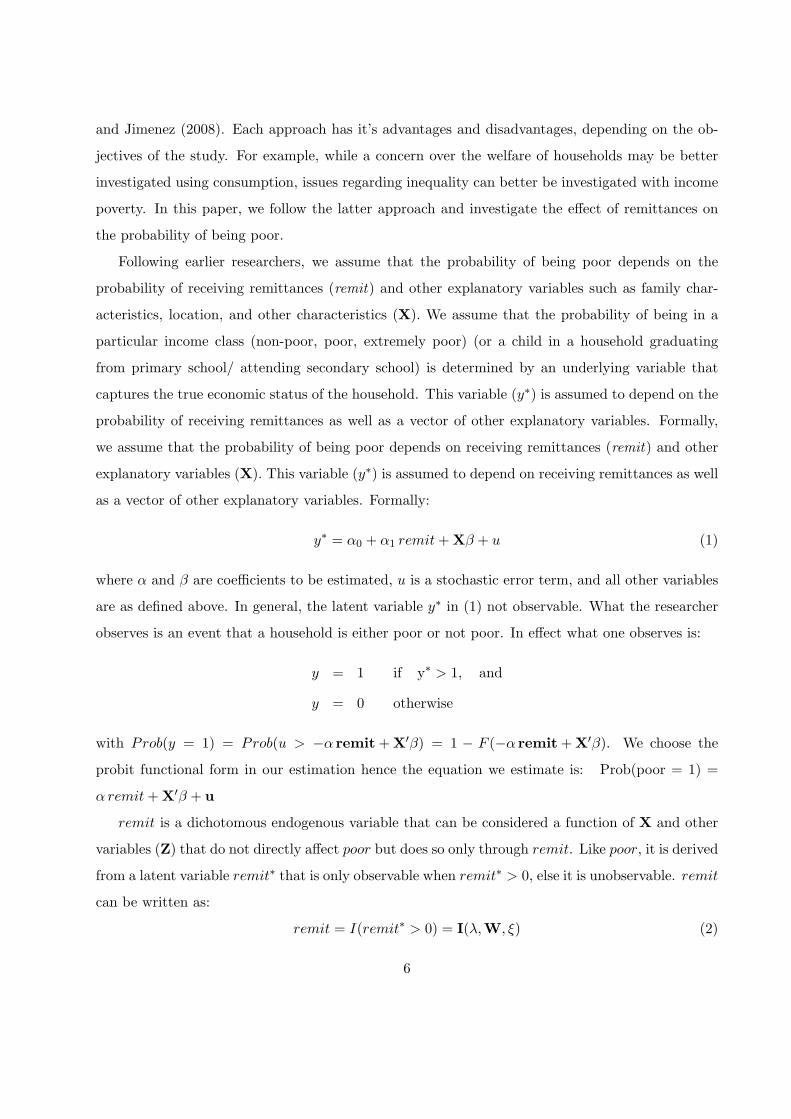
with Prob(y = 1) = Prob(u > −α remit + X′β) = 1 − F (−α remit + X′β). We choose the

probit functional form in our estimation hence the equation we estimate is: Prob(poor = 1) =

α remit + X′β + u

remit is a dichotomous endogenous variable that can be considered a function of X and other

variables (Z) that do not directly affect poor but does so only through remit. Like poor, it is derived

from a latent variable remit∗ that is only observable when remit∗ > 0, else it is unobservable. remit

can be written as:

remit = I(remit∗ > 0) = I(λ,W, ξ) (2)

6

where W = X + Z. Substituting remit into the y equation, one can write y as:

y = I(y∗ > 0)

= I(α (X + Z + ξ) + X′β + u ≥ 0)

= I(αλ,Z + Z′( α + β) + ξ + u ≥ 0)

= I(Z,X, β, γ, ζ ≥ 0)

where γ = λ ∗ α and ζ = U + ξ. In this set up the effect of remit on poverty incidence is given

as..

We follow earlier researchers in determining the variables contained in the X vector. These

include the education of the head of the household (education), the age of the head of the household

(age) and its square (agesq), the gender of the head of household (gender), number of adult workers

in the household (workers), household size (hhsize) and rural location (rural). In addition, we

include an ethnic variable, whether a household belong to the Asante ethnic group (asante). This

ethnic group has an extensive migration network and their cultural heritage requires the younger

generation to take care of their elderly as well as participate in civic projects. This implies that

they will be more likely to help other members of their households by taking measures to help

reduce poverty. Because we are interested in the effect of international remittances on household

poverty, we break total remittances (remit) into domestic remittances (domestic) and international

remittances (abroad).

The equation we estimate is given as:

Prob(poor = 1|X) = α1 domestic + α2 abroad + α3 age + α4 agesq + α5 gender

+ 6 asante + α7 workers + α8 hhsize + α9 rural + α10 education (3)

+ β11 gender ∗ abroad + ε

where ε is a stochastic error term and all other variables are as defined above. In addition to the

variables discussed above, we have also included an interaction term between gender and abroad to

see if there is a gender difference on the effect of remittances on the probability that a a household

will be poor, all things equal. If remittances decreases the probability that a household will fall

into poverty, we expect the marginal effect of domestic and abroad to be negative, all things equal.

We also expect the marginal effect of the gender/abroad interaction term to be significant if there

is a gender difference in the effect of international remittances on household poverty in Ghana.

7

3.2 Estimation Method

We estimate (3) with two data sets—cross-section sample based on GLSS5 and a pseudo-panel

data set constructed from GLSS3-GLSS5. Efficient estimation from each data may require different

estimation method. We therefore briefly describe the estimation methods used for each data set in

this section. Sub-section 1 describes the method for estimation with the cross-section data while

sub-section 2 discusses the estimation method used for the pseudo-panel data.

3.2.1 Cross-section estimation

Estimating equation (3) will be straight forward with a probit estimator if all regressors were

exogenous. If there is a continuous endogenous regressor, one could use standard instrumental

variables (IV) two stage probit estimator to estimate the equation. In our study, remit is a

binary endogenous variable that cannot be represented by the standard linear IV approach in a

probit estimation strategy since remit is non-linear and linear IV representation will also lead to

heteroskedastic errors. Under these circumstances the two stage probit estimation of poverty is not

appropriate as Carrasco (2001) points out.1 Because the dependent variable (poor) is binary and

one of the regressors (the one of major interest) is also binary, we have a bivariate probit model in

which the regressor of interest (remit) is binary and endogenous. Our approach to the solution of

the problem posed by the endogeneity of remit follows the approach suggested by Carrasco (2001).

The solution is to specify a reduced form probit equation for remit of the following form:

remiti = I(remit∗i > 0)

= I(λ0 + λ1X + λ2Zi + εi > 0)

where εi is a normally distributed error term, Z is a vector variables that affect poor only through

remit and X is as defined above. The key to identification in this set up is to find a set of

regressors in the remit equation that affect remit but does not directly affect poor. In this paper,

we use migrant networks (networks) and the number of remitters (remitters) as instruments for

the probability of remittances from abroad. These variables meet the criteria for appropriate

instruments developed by McKenzie and Sasin (2007).

We instrument for abroad as discussed above in estimating the poverty equation. We measure

migrant networks (networks) as the number of people in the community (town/neighborhood)

who have migrated in the last 5 years and the number of people who have sent remittances to the

8

household in the past (remitters) as instruments. We used the CMP routine in STATA written

by Roodman to implement this this bivariate probit estimation. The CMP routine is a maximum

likelihood estimator that is flexible enough to allow for several estimators, including the bivariate

probit. CMP estimates the bivariate probit model recursively; while abroad is allowed to affect

poor, poor does not affect abroad.

While we use bivariate probit to estimate the poverty equation when we measure poverty as

poor, we use ordered bivariate probit estimator to estimate the poverty equation when we measure

poverty as pstatus since it is ordered and takes on the value 0, 1, and 2, where 0 indicates extreme

poverty, 1 indicates moderate but not extreme poverty, while 2 indicates not poor. As indicated,

we instrument for both poor and pstatus in our estimation. In the bivariate ordered probit, we

set the probability of being poor or not poor to zero, in the estimation and use the estimate as an

instrument. In the education equation, we measure the dependent variable as the proportion of

children in a household who have completed primary school or are enrolled in a secondary school,

the variable is censored both from above and below and it is possible that there are a lot zero

primary school completion rates.

3.2.2 Pseudo-panel Estimates

In estimating (4) with individual household data, a bivariate probit estimator is called for since

both the depended variable and the endogenous regressor both take the value of 0 or 1. When one

estimates the equation using a pseudo-panel data, the cohort means of both the dependent variable

and the endogenous regressor are non zero but continuous although they may be censored. In this

case the bivariate probit estimator is not appropriate for the estimation for the poor equation. An

estimator with a non-limited dependent variable is the appropriate estimator for estimating the

poor equation using pseudo-panel data.

In pseudo-panel data setting, one cannot use either the first difference or the fixed effects

estimator since the sample household differs from one wave to the next and therefore one cannot

estimate an individual fixed effects. On the other hand, individual errors are likely to be correlated

with regressors in any wave, making the random effects (RE) estimator inconsistent. Deaton has

suggests creating a panel of cohorts and using the cohort means as individual observations for

estimation with appropriate panel estimator. Since the cohort means are not likely to represent the

population means with errors, Deaton’s estimator is an errors in variables estimator. The estimator

9

produces consistent estimates if the cohort sizes are the cohort sizes are large and the selection into

cohorts do not change over time. In addition, in our setting, we have an endogenous regressor in

abroad, hence this estimator may not be appropriate.

The Deaton estimator is based on group averages for the cohorts. Taking group time averages

for equation (4), the pseudo-panel model can be written as:

¯poorst = αst + δs + β′Wst + εst (4)

where ¯poorst, Wst are group means of the dependent and explanatory variables for group s at time

t, αst group specific fixed effect for group s at time t, s in time invariant group specific group effects

for group s, εst is the mean error term for cohort s at time t, and β is a vector of coefficients

to be estimated. The moment restrictions required for the estimation of this equation is that the

group section variable (i ∈ IN,st) is orthogonal to the error term αi + εi, where I(.) is and indicator

function that selects into group st. Formally, the moment conditions necessary for FE or a GMM

estimator to be used to estimate this equation is: E(αi +εi|i ∈ I1t(s)) for all T and S. For relatively

large cohort sizes, Deaton suggests either a least squares estimator or a fixed effects (FE) as the

appropriate estimator for such a pseudo-panel model.

Several authors have suggested that Deaton’s estimator may be inconsistent or produce inef-

ficient estimates when time invariant group fixed effects are not appropriately accounted for. In

addition, we treat abroad as an endogenous regressor, it is unlikely that the FE estimator will be

appropriate for purposes. In the presence of a binary regressor, some authors have suggested using

a linear probability estimator to estimate the first stage and use a probit in the second stage.2

Recent research has argued that the first stage linear probability estimator is inappropriate since

there is no guarantee that the estimated linear probability in the first stage will lie in the [0 1]

range; moreover the assumption of linear marginal effects may not be appropriate. Even if it did,

the linear probability introduces heteroskedastic errors in the endogenous regressor. These authors

have suggested various GMM estimators. Inoue (2008) has suggested that Deaton’s least squares

estimator produces estimates that asymptotically converges to a random variable while the fixed

effects estimator is consistent but inefficient. He suggests a GMM estimator that is robust to the

existence of time invariant group fixed effects and also efficient. This estimator is derived from

the orthogonality conditions implied by the grouping to create the cohorts. We use the estimator

suggested by Inoue.

10

The Inoue GMM estimator is given as:

βGMM = (W′Ω−1W)−1W

′Ω−1y (5)

where W is the S(ST − 1)× (K + L) matrix obtained from deleting the Tth, 2Tth...ST th rows of

MW, where W a matrix of regressors, M is a set of orthogonality conditions obtained from forming

the cohorts, Ω is the variance covariance matrix of ε adjusted for cohort sizes, and y are the cohort

means of the dependent variable. This estimator can be modified to account for heteroskedasticity

and autocorrelation. Inoue shows that even when the FE and the GMM estimators are based on

the same moment conditions, the GMM estimator is efficient because it is based on the optimal

weighting matrix and is preferred to the FE estimator. We calculate Hansen’s J statistic to check

for over identifying restrictions in our estimation.

4 Data

The data used for this study comes from wave 5 and waves 3-5 (for pseudo-panel) of the Ghana

Living Standard Standard Surveys (GLSS). Beginning in September 1987, Ghana with the help of

the World Bank, has conducted surveys of living standards of large nationally representative samples

of households at regular intervals. GLSS1 was conducted in 1987/1988, GLSS2 was conducted in

1988/89, GLSS3 was conducted in 1991/1992 and covered the entire country with a sample of

4552 households in all 407 enumeration areas; GLSS4 was conducted in 1998/1999, covered the

entire country and had a sample of 6,000 households while GLSS5 was conducted in 2005/2006,

covered the entire country with a sample size of 8,687 households. It appears that each wave of

GLSS covered more households as well as provided more detailed and comprehensive information

about the living standards of Ghanaian households than previous ones. Besides the increasing

detail regarding information provided in succeeding waves, one difference between GLSS3 on the

one hand and GLSS4 and GLSS5 on the other is the absence of information about Upper East and

Upper West administrative regions which were carved out of the old Upper Region of Ghana in

1983.

These surveys contain detail information on socio economic characteristics of households, eth-

nicity, gender, household size and composition, income, employment, consumption, and educational

attainment, among other variables. These surveys also have information on whether households

receive remittances, source of remittances (internal or international), amount of remittances, as well

11

as the disposition of remittances, including consumption, private and public investment projects, as

well human capital formation (health and education). The detailed nature of the survey data allows

us to investigate the effects remittances on poverty status and human capital formation. We are

not able to use data from GLSS1 and GLSS2 because the surveys did ask detailed questions about

remittances as well as some of the socioeconomic variables necessary to estimate the equations.

The variable of main interest in this paper is remittance. The GLSS provides information

on whether households receive remittance or not; and if so whether the remittance is from within

Ghana (domestic) or from outside Ghana (abroad), whether these remittances are cash remittances

or remittances of goods, as well the monetary value of such remittances. We measure remittance

as the sum of monetary value of cash and good remittances received by households in a year.

Because we are interested in the effects of international remittances on poverty status of Ghanaian

households, we break remittances into domestic and international (abroad) remittances. Although

the GLSS asks questions about the amount of remittances received by a household, because of

recall problems, it is most likely that the amount will be measured with a large error. Moreover,

the questionnaire is administered to the head of the household and while she/he may accurately

recall the receipt of a remittance to another member of the household, she/he is unlikely to recollect

the amount of the remittance with much accuracy. We therefore measure remittance as whether a

household receives a remittance in a year without regard to the size of the remittance. However, we

make a distinction between the probability of receiving remittance from within Ghana (domestic)

and international (abroad).

The dependent variables we are interested in are the poverty incidence and school attendance.

We measure poverty incidence in several different ways. First, we measure poverty as the proba-

bility that a household falls into poverty based on defined poverty lines.3 The lower poverty line

(POOR0) is set at C700,000.00 with 199/99 as the base while upper poverty line (POOR1) is

set at C900,000.00. This is consistent with the headcount measure of poverty. Second, we use

the poverty lines to calculate poverty gap (POV GAP ) as well as the square of the poverty gap

(POV GAPSQ) based on the lower poverty line as additional measures of poverty. It is well known

that the headcount measure of poverty does not adequately capture the severity of poverty. These

additional measures of poverty are intended to capture these aspects of poverty. In addition to

these additional measures of poverty, we also include consumption as additional measures of house-

hold welfare. We measure human capital investment by the proportion of children in a household

12

that are enrolled or completed primary school (PRIMARY ) or enrollment in secondary school

(SECONDARY ).

We measure education (education) as the highest level of education attained by the head of

the household where education is coded as follows: none = 0, primary = 1, technical, vocational

= 2, secondary, teacher training A & B = 3, SSCE, GCE A level, teacher training post sec = 4,

polytechnic = 5, bachelors = 6, masters = 7, doctorate = 8. Age (age) is the age of the head of

the household, workers (workers) is the number of adult workers in a household, household size

(hhsize) is measured as the total number of people in a household, gender is an indicator variable

that takes the value 1 if the head of the household is male, zero otherwise, asante is an indicator

variable that equals unity if the household belongs to the Asante ethnic group, zero otherwise,

while rural (rural) is a dichotomous variable that equals 1 if the household lives in a rural area,

zero otherwise.

Sample statistics of the cross-section data from GLSS5 used for estimating the model are pre-

sented in table 1. The sample statistics suggest that about 24% households in the sample are

poor. This poverty rate is further sub-divided into 16.04% extremely poor and 8.05% moderately

poor. The 24.09% poverty rate in GLSS5 is a strong improvement over the poverty rate of 39.5%

estimated in GLSS3.4 Heads of households in the sample are predominantly male (72%), while the

average household has 4.2 members with a very large variation. Similarly, the average houshold

head is 42.34 years old with a very large range (15 – 99 years) in age. 58.4% of the households in the

sample reside in rural areas compared to about 41.6% living in urban areas. Themean educational

attainment of household heads in the sample is low. About 31% of all household heads have no

formal education, another 33% has only primary education; on the other hand only about 3% of

household heads had the equivalent of a bachelors degree or more. About 29.8% of households

in the sample received some form of remittances from within Ghana (domestic) while only about

6.9% of households received international remittances (abroad). The mean amount of domestic

and abroad are C 1,687,258.00 and C 7,777,685.00 respectively indicating that the average amount

international remittance is about five times that of domestic remittance.5

Some comments on the characteristics of the sample data, summarized in table 2, are in order.

Of the 24.09% of households in poverty in 2006, fully 86.3% lived in rural areas. Compared to

the proportion of rural households in the sample (58.4), the proportion of poor households in rural

households suggests that poverty in Ghana is a predominatly rural phenomenon. Surprisingly,

13

a larger proportion of male-headed households were more likely to be poor than female headed

households. Only 15.89% of female headed households were poor compared to 27.25% of male-

headed households. This may partly be explained by the dominance of male-headed households

in the sample from the three poor northern regions of Ghana. Nationally, the data indicates that

72.12% of households in the sample are headed by males and on average, 24.09% are poor. In the

three poor northern regions, 85.92% of households are headed by men and the average poverty

among households in these three regions is 64.41%. Unlike Quartey and Blankson (2004) who find

that female headed-headed households were less lkely to receive remittances compared to the male-

headed households, we find that female-headed households are more likely to recieve rimttances both

from Ghana and abroad. While 24.49% and 5.67% of male-headed households received remittances

from within Ghana and abroad respectively, 44.01% and 11.15% of female headed households

received domestic and foreign remittances respcetively. While it is true that in absolute terms, fewer

female-headed households recieved rimttances compared to male-headed households, in relative

terms, female-heades households have a higher probability of receiving international remittances

than male-headed households.

While the sample data described above is based on the latest wave of GLSS (GLSS5), the

pseudo panel data we construct and used for the pseudo panel data portion of the study is similarly

structured. Deaton (1985) suggests creating cohorts based on some pre-determined characteristics

that are time invariant. In building the pseudo-panel panel data set involves a trade off between the

size of a cohort and the number of cohorts. Increasing the number of cohorts decreasing the average

size of a cohort thus increasing the chance that the cohort means do not represent the population

characteristics of that cohort. On the other hand, increasing the size of each cohort decreases the

number of cohorts leading to inefficient estimates on account of possible lack of variation across

cohort means and small sample size. We created cohorts based on the year of birth, gender, and

location (rural or urban). We created 5 year birth year bands, two locations (rural and urban),

and two gender categories (male/female). With 8 birth years, two locations and two genders, we

obtained 32 cohorts for each wave for a total sample of 96 cohort observations.

The distribution of cohort sizes are presented in table 3. The average sample size for a cohort

is 196.96 with a minimum of 88 and a maximum of 538. In general, the average cohort sizes are

larger fro male-headed rural household while they are smallest for female-headed urban households

regardless of the age bracket one looks at. This is partly due to the fact that there are more male-

14

headed households in Ghana than female-headed households and the GLSS generally samples more

rural households than urban households. Finally, younger cohorts are over-represented compared

to older cohorts in the data. Another characteristic of the data is that poverty rates are higher

in older, male-headed, rural cohorts than their female-headed, younger urban cohorts. The data

also show that conditional on on year of birth and gender, urban cohorts are more likely to receive

external remittances compared to rural cohorts. Even though we measure poverty as the probability

that a household falls into a category of poverty, the cohort means are never zero hence these cohort

means are essentially continuous variables.

5 Results

This section presents the estimates of equation (3) using both the cross-section data from GLSS5

and the pseudo-panel data constructed from GLSS3-GLSS5. The first subsection presents the

estimates for the poverty equation while the second subsection presents the estimates for the school

enrollment equation. The first part of each sub-section presents the estimates based on the cross-

section data while the second section presents the estimates from the pseudo-panel data.

5.1 Poverty

5.1.1 Cross-Section Estimates: GLSS5

Estimates of the marginal effects of the various regressors on poverty rate based on the cross-section

data are presented in tables 4 and 5. Columns 2 and 3 present the estimates of the probability of

being poor which is a combination of the probability of being moderately poor and the probability of

being extremely poor. Column 2 presents the estimates without a gender/abroad interaction while

column 3 presents the estimates that includes the interaction term. Because this is single outcome

event, we use a simple bivariate probit estimator to estimate the equation. Columns 4-6 present

the estimates of poverty status (pstatus) which ranges from extreme poverty, moderate poverty

to not poor. Because poverty status is ordered, we use an ordered bivariate probit estimator to

estimate the equation. Regression statistics indicate that the model generally fits the data well. In

all regressions, we reject the null hypothesis that all variables jointly have no significant on poverty

probabilities at α = .01 and we are unable to reject the null that the model is correctly specified.

Finally, the estimated marginal effects have the correct signs and are significantly different from

zero at conventional levels. The last two rows in table 4 show the the estimated equation have

15

reasonably good predictive ability.

The marginal effects of abroad in columns 2 and 3 is negative and significant at α = .01 or

better. This estimate suggests that international remittances have a significantly negative effect

on the probability of a household being poor, all things equal. The estimates in column 2 suggest

that the probability of of household being poor decreases by 0.10 when a household that did not

previously receive a remittance from abroad receives a remittance from abroad, all things equal.

The marginal effect of receiving an international remittance is relatively large; it is about 6 times

the effect that education has on poverty incidence on Ghanaian households, all things equal. On

the other side, it is large enough to completely eliminate the effects rural location on poverty

incidence among households. In column 2, the marginal effects of domestic is negative, very small

but statistically significant at α = 10. This indicates that remittances from domestic sources have

statistically significant impact on the probability of a household being poor. Does the gender of

the recipient of international remittance makes a difference on its effect on poverty incidence? The

marginal effect of gender ∗ abroad is negative but insignificant at conventional levels, suggesting

that the gender of the household head of recipient of international remittance has significant impact

of poverty incidence among Ghanaian households, all things equal.

The marginal effects of education and age are negative significant at α = .01 suggesting that the

probability of a household being poor decreases with the educational and age of the household. On

the other hand, the coefficient of agesq is positive and significant. The combination of the marginal

effects of age and agesq suggests that age of the household head decreases the probability of a

household being poor at a decreasing rate. The marginal effects of workers, hhsize and rural are

positive and significantly different from zero at α = .01. These effects suggest that the probability

that a household falls into poverty increases with the size of the household, the number of adult

workers in the household, and rural location. These effects are consistent with our expectation and

are similar to those found by earlier researchers (Glewe: 1991, Castaldo and Reilly: 2007, Acosta

et al: 2008, Grootaert: 1997, Mukherjee and Benson: 2003, among others). The marginal effect of

gender is positive but insignificant at any reasonable confidence level suggesting that male-headed

households are no more/or less likely to be poor than female headed households. This estimate

is counter intuitive and inconsistent with the results of previous studies that finds that male-

headed households are less likely to be poor compared to female-headed households. However,

as discussed above, male-headed households overwhelmingly dominate in the poorest regions in

16

the sample where on average about 66% of households are poor. This dominance of male-headed

households in the poorest regions of the Ghana may be driving the coefficient on gender. The

marginal effect of asante is negative and significantly different from zero, suggesting that Asante

ethnicity is negatively correlated with poverty incidence.

In columns 2 and 3, we measure poverty as the probability of being poor. It is possible that

remittances affect moderate poverty probability differently from the way it affects extreme poverty

probability. We present estimates for poverty status (pstatus) where poverty status takes on the

values extreme poor (poor0), moderately poor (poor1) and not poor (notpoor). Estimates of the

marginal effects of poverty status equation are presented in columns 4-6 in table 4. Given the

way poverty status is coded, we expect the coefficients in column 6 to be opposite in signs to

their counterparts in columns 4 and 5. The marginal effect of abroad in columns 4 and 5 are

negative, relatively large and significantly different from zero at α = .01 while the marginal effect

of that variable in column 5 is positive and significant. These coefficient estimates indicate that

international remittances decrease the probability that recipient households will be either extremely

or moderately poor; on the other hand, it increases the probability that these households are not

poor. The marginal effects of abroad on the probability of being extremely poor and moderately

poor are similar in magnitude.6 The marginal effects of domestic in columns 4 and 5 are negative

but insignificant while it is positive and significant in column 5 suggesting that domestic remittances

have no significant impact on the probability of a household being moderately poor or extremely

poor but has a significantly positive effect on not being poor. The marginal effect of the other

variables in columns 4 and 5 are similar in sign and statistical significance as their counterparts in

column 2 while the estimates in column 6 are opposite in signs as their counterparts in column 2-5

but are equally significant as those estimates. The estimates in column 4-6 confirm the results we

obtained in columns 2 and 3 and suggest that our results are robust to the level of poverty that is

measured.

The estimates in table 4 are based on the headcount measure of poverty which does not reflect

differences in the severity of poverty. In table 5, we present estimates of the poverty equation based

on two measures of poverty—poverty gap and the square of poverty gap. We calculated two sets of

poverty gaps and their squares—based on the high income poverty threshold of C900,000.00 and

the other based on expenditure threshold. Columns 2 and 3 in table 5 present the estimates for the

gap and gapsq based on income poverty while columns 4 and 5 presents the same sets of estimates

17

for poverty calculated from expenditure. We note that because gapsq are conceptually different

from gap and headcount measures, the marginal effects are likely to be different and opposite in

signs to those of the gap measures. In columns 2 and 4, the marginal effects of abroad is negative

and significant at α = .01 indicating that international remittances decreases the probability of a

family being poor as measured by the gap approach. The marginal effects of abroad is positive

and significant in the incgapsq and expgapsq equations in columns 3 and 5 indicating that receipt

of external remittance have significant impact on poverty rates among Ghanaian households. The

marginal effects of all other variables are similar in sign, statistical significance, and interpretation

as their counterparts in table 3. We conclude that our results that international remittances reduces

poverty incidence among Ghanaian households is robust to the measurement of poverty.

5.1.2 Pseudo-Panel Data Estimates

Are our results different when we move from cross-section data to panel data estimates? The

pseudo-panel data estimates of the poverty equations are presented in table 6. We do not include

gender as a regressor in the pseudo-panel estimates since we use it to construct the cohort. However,

we include the interaction between gender and abroad to test for the existence of gender effects on

the relationship between abroad and poverty. Column 2 presents the estimates when we measure

poor as the probability of being poor, column 3 present the estimates when we measure poverty

as the probability of being in a particular income class (pstatus), while columns 4 and 5 present

the estimates based on income poverty gap and consumption poverty respectively. The regression

statistics indicate a reasonably good fit to the data. We reject the null hypothesis that all regressors

jointly do not contribute to the explanation of poverty at α = .01. The Klienbergen-Paap LM test

for identification indicate strong instruments while the Hansen J test of over-identifying restrictions

suggest that our instrument vector is appropriate.

The marginal effect of abroad is negative, relatively large and significantly different from zero

at α = .01 indicating that international remittances have a significantly large negative effect on

the probability that a household falls into poverty, all things equal. These marginal effects are

qualitatively similar to those presented in table 4 for the GLSS5 data. The only difference between

the two estimates is the larger magnitude of the estimate of abroad in table 6, compared to its

counterpart in table 4. The marginal effects of domestic in column 2 is negative and significant at

α = .10 indicating that domestic remittances reduce the probability of a household being poor, all

18

things equal. The marginal effect abroad ∗ gender is positive and significant suggesting that there

is a significant gender effect of international remittances on poverty. All things equal, the ability of

international remittances to decrease the probability of a household being poor is higher for female-

headed households than male-headed households. We conclude that our result that international

remittances decrease poverty among Ghanaian households is robust to the data—cross section or

pseudo-panel—used to estimate the poverty equation.

The marginal effects of education, asante, workers are negative and significant at conventional

levels while the marginal effects of rural and hhsize are positive and significant at α = .01,

indicating that poverty incidence among Ghanaian households decreases with education, number of

workers in the household, and Asante ethnicity while it increases with rural location and household

size. These estimates are similar to the estimates in table 4. The marginal effects of age is

negative while that of agesq is positive but they are insignificant at conventional levels. Although

these coefficient estimates are insignificant, they have the same signs as their counterparts in the

cross-section estimates presented in table 4. The poverty status estimates are presented in column

3. Because pstatus is coded in such a way that higher values imply less poverty, the signs of

the coefficients will be opposite of their counterparts in column 2. The coefficients of domestic

and abroad in column 3 are positive and significant as expected, indicating that increases in these

variables increase the probability of a household not being poor. These estimates are consistent with

their counterparts in column 2. Again, this confirm our conclusion that international remittances

have a negative and statistically significant effect on poverty incidence in Ghana, all things equal.

The marginal effects of education and workers are positive and significant while those of rural

and hhsize are negative and significant. The estimates are consistent with their counterparts in

column 2. The coefficients of age, agesq, and asante are insignificant, although they all have the

expected signs.

The estimates based on gap measures of poverty are presented in columns 4 and 5. Column

4 presents the estimates for the income gap while column 5 presents the estimates for the expen-

diture gap. The signs and statistical significance of these estimates are remarkably similar their

counterparts in column 2. In particular, the coefficient of abroad is negative and significant in

both columns, suggesting that our results do not depend on how we measure poverty: regardless

of the measure of poverty, international remittances have a statistically significant impact on its

incidence on Ghanaian households. The signs and statistical significance of the coefficients of the

19

other variables are also similar to their counterparts in the cross-section estimates. We therefore

conclude that international remittances have a strong negative and stable effect on the propensity

of households to fall into poverty, all things equal and that our results do not depend on the data

set we use to estimate the equation.

5.2 Education

The coefficient of abroad in both columns 2 and 3 is positive and significant suggesting that in-

ternational remittance has positive and significant impact on primary school completion rate and

secondary school enrollment rates. These are relatively large effects. For example, conditional on

holding all other variables constant at their means, the probability that a child in a Ghanaian

household attend/complete primary school or enroll in secondary school increases by 0.09 and 0.49

respectively when a household changes from non recipient to a recipient of international remit-

tance. The gender/abroad interaction term (abroad∗ gender) has negative and significant effect on

primary education but a positive and insignificant effect on secondary school enrollment rate, sug-

gesting that male-headed households who receive international remittances are less likely to enroll

their children in primary school compared to female-headed households who receive international

remittances. The policy implication is that remittances to female-headed household is more likely

to lead to human capital formation hence long term poverty reduction compared to remittances to

male-headed households. This result is consistent with the results obtained by earlier researchers

who find that females are more likely to use remittances take care of children than males, all things

equal.

The estimates of the effects of international remittances on education are presented in table

7. Columns 2 and 3 present the estimates for primary school and secondary school enrollment

using the cross-section data while columns 4 and 5 present their pseudo-panel counterparts. Re-

gression statistics indicate a relatively good fit and the estimates are of the expected signs and

generally significant. The coefficients of education, age, gender, the logarithm of income are posi-

tive and statistically significant in columns 2 and 3 indicating that these variables have positive and

significant effects on primary school enrollment or completion rates and secondary enrollment prob-

abilities among Ghanaian households. The coefficient of asante is positive but only significant in

the primary school completion equation. The coefficient of rural is negative and significant indicat-

ing that primary school completing rates and secondary school enrollment rates among Ghanaian

20

households are lower in rural locations.

The pseudo-panel estimates for education are presented in columns 4 and 5 of table 7. Column

4 presents the estimates for primary school enrollment/completion while column 5 presents the

secondary school enrollment rate. Regression statistics indicate a good fit to the pseudo-panel

data. In particular, both the Kleinbergen-Paap LM test and Hansen J test indicate strong and

appropriate instrument vector. The estimated coefficients are generally of the expected signs and

are generally statistically significant.

The coefficient of abroad in columns 4 and 5 is positive, relatively large and significantly dif-

ferent from zero at α = .01 or better. This estimate suggests that, all things equal, Ghanaian

households that receive international remittances are more likely to enroll their children in primary

and secondary school in the medium to long run. The estimate of the interaction term between

gender and abroad is negative, relatively large, and significant in both columns 4 and 5. This gen-

der effect suggests that female headed households that receive international remittances are more

likely to educate children in the household than male-headed households that receive international

remittances. These estimates are similar to their cross-section counterparts in columns 2 and 3.

Perhaps, the only difference between the two sets of estimates is the relatively large magnitudes

of the panel estimates. Of course it is known that the two sets of estimates are only comparable

in direction but not magnitude. In addition to the coefficient of abroad, the coefficients of other

variables in the equation—education, age, log of income, domestic—are positive and significantly

different from zero α = .05 or better. The only variable that is insignificant in the pseudo-panel

equation is asante. We can conclude from this subsection that international remittances do have a

positive and significant impact on education human capital formation in Ghanaian households and

this result does not depend on the data used for estimation.

5.3 Policy Implications

Our results that international remittances significantly reduces poverty incidence among Ghanaian

household is similar to the results of other researchers who have investigated the relationship

between poverty and international remittances in Ghana (Adams: 2006a, Guzman et al : 2006,

Litchfield and Waddington: 2003, Quartey and Blankson: 2004, Quartey: 2006) as well as those

who have investigated the relationship elsewhere (Grootaert: 1997, Niimi et al : 2009, Mukherjee

and Benson: 2003, Acosta et al : 2008, Adams: 2004, Brown and Jimenez: 2008, and Castaldo and

21

Reiley: 2007). Our results are also consistent with the results of studies that find that women are

more likely to use remittances to take care of children than men who receive remittances, all things

equal. We note that our results stand both in the short- and long-runs.

Our results have both policy and research implications. First, the results that international

remittances reduces the incidence of poverty among Ghanaian households suggests that Ghanaian

policy makers encourage their citizens in the Diaspora to increase the flow of remittances to Ghana

through appropriate policy reforms. Specifically, policies to reduce the transaction cost, such as

excessive bank and other transfer changes, associated with sending international remittances to

Ghana make in order.7 In addition policy makes should provide incentives, such as paying reasonable

interest or providing safe and profitable financial instruments to attract more remittances to Ghana.

The gender differences on the effects of international remittances also have implications not only for

those who send remittances to Ghana but for the long term development of Ghana generally. Since

remittances sent to female headed household increases the probability of human capital formation

compared to remittances to male-headed households, it implies that Ghanaians in the Diaspora

sending remittances to their relatives should channel more of the remittances to female members of

their households if their objective is to increase human capital formation and hence reduce poverty

in their household the long run as well as contribute to Ghana’s long-term development.

Previous studies have used either a simple probit estimator for cross-section data or the least

squares of fixed effects estimator for pseudo panel data to investigated the effects of remittances on

poverty in LDCs. However, the endogeneity of remittance (see McKenzie and Sasin: 2007) suggests

that these estimators are not appropriate. Our results implies that researchers could use estimators

that can account for endogeneity of remittances as well as cohort fixed effects to obtain efficient

estimates. A large proportion of studies of the effects of remittances on welfare has focused on

the effects on current consumption or current income. The direct effect of remittances on current

consumption does not indicate the effect of such remittances on poverty in the long run. On the

other hand, the effects of remittances on human capital formation may give an indication of the long

term effect of remittances on poverty given that a major determinant of poverty in a household is

the quantity and quality of human capital endowments of its members. Perhaps, researchers should

focus a little more attention on the effects of remittances on human capital formation rather than

the major focus on its effect on current consumption and income. Finally, we find a significant

gender difference in the effects of remittances on education. Perhaps, researchers may need to

22

investigate other differential effects, such regional differences or locational differences (urban versus

rural) in order to provide policy makers more detailed policy information.

6 Conclusion

This paper uses two sets of data—cross-section data from GLSS5 and pseudo-panel data set con-

structed from GLSS3-GLSS5—a bivariate probit and pseudo-panel GMM estimators to investigate

the effects of international remittances on poverty incidence and primary and secondary educa-

tion in Ghana. Controlling for several covariates, we find that international remittances have a

significantly negative impact on the probability of a household being poor. We also find that in-

ternational remittances increases the chances that a household will educate its young members,

at least through primary and secondary school, all things equal, suggesting that international re-

mittances have positive impacts on human capital formation, hence long term poverty reduction

among households as well the long term growth of the Ghanaian economy. We also find that there

is a gender difference in the effect of international remittances on human capital formation: con-

ditional on receiving international remittances, male-headed households are less likely to educated

their children than female-headed households. Our results are robust to the type of data used

(cross-section or pseudo-panel) the measurement of poverty (headcount, poverty gap, poverty gap

squared), as well as the estimation method (bivariate probit or pseudo-panel GMM).

An implication of our results is that increasing the flow of remittances to Ghana can significantly

decrease poverty rates among households and increase educational attainment of the young members

of recipient households. Another implication of our results is that while increasing remittances to all

Ghanaian households decreases poverty in the short run, it makes a significance difference in human

capital formation and long term poverty reduction whether the recipient household is headed by a

male or a female. Female-headed household that receive international remittances are more likely to

educate their children compared to male-headed households who receive international remittances.

Our results have interesting and important policy implications.

23

7 Notes

1. See Carrasco (2001) and note 2 below.

2. Although Angrist (2001) suggests that researchers should worry more about drawing causal

inference when they are faced with binary endogenous regressors rather than the “appropriate”

estimation method, many authors argue that with the appropriate estimator, the wrong inference

will be drawn from such estimates.

3. The poverty line is defined as total household consumption expenditure per adult equivalent

expressed at in constant prices.

4. The moderate and extreme poverty rates estimated in GLSS3 are 12.7% and 26.8% respectively

while the comparable rates for GLSS4 were 10.30% and 18.20% respectively. These figures sugges

that consistent reduction in the poverty rate in Ghana in recent periods. Of course, the reduction

in poverty incidence could be due to several factors, including sample selection over the various

surveys.

5. The mean Cedi/Dollar exchange rate in 2006 was C9,550.00 indicating that the mean amount

of domestic and international remittances were approximately $170.00 and $782.00 respectively.

6. Note that the marginal effects of abroad across the various poverty status (poor - poor2) sum to

zero since the probability of poverty status sum to unity.

7. Currently, Ghanaian banks require one to maintain two separate accounts—one to receive foreign

deposits and the other to withdraw money—in order to send and use remittance to Ghana. One

pays money into the receiving account, then ask the money to be transferred into the paying

account before one can withdraw money from the paying account. Each of these accounts attracts

a transaction fee—a fee to pay into the receiving account and another fee to withdraw on the

account.

24

8 References

1. Acosta, P., C. Calderon, P. Fajnzylber, and H. Lopez (2008), “What is the Impact of Inter-

national Remittances on Poverty and Inequality in Latin America?” World Development, 36 (1),

89-114.

2. Adams, R. H. (2004), Remittances and Poverty in Guatemala, World Bank Policy Research

Working Paper No. 3418.

3. Adams, R. H. (2006a), Remittances and Poverty in Ghana, World Bank Policy Research Working

Paper No. 3838.

4. Adams, R. H. (2006b), “International Remittances and the Household: Analysis and Review of

Global Evidence”, Journal of African Economies, 15, AERC Supplement 2, 396-425.

5. Adams, R. H. (2008), The Demographic, Economic and Financial Determinants of International

Remittances in Developing Countries, World Bank Policy Research Papers, No. 4583.

6. Angrist, J. (2001), “Estimation of Limited Dependent Variable Models with Dummy Endogenous

Regressors: Simple Strategies for Empirical Practice”, Journal of Business and Economic Statistics,

19 (1), 2-16.

7. Azam, J-P and F. Gubert (2006), “Migrants’ Remittances and the Household in Africa: A

Review of Evidence”, Journal of African Economies, 15, AERC Supplement 2, 426-462.

8. Brown, R. P. C. and E. Jimenez (2008), “Estimating the the Net Effect of Migration and

Remittances on Poverty and Inequality: Comparison of Fiji and Tonga”, Journal of International

Development, 20, 547-571.

9. Carrasco, R. (2001), “Binary Choice with Binary Endogenous Regressors in Panel Data: Esti-

mating the Effects of Fertility on Female Labor Participation”, Journal of Business and Economic

Statistics, 19 (4), 385-394.

10. Castaldo, A. and B. Reilly (2007), “Do Migrant Remittances Affect the Consumption Patterns

of Albanian Households?”, South-Eastern Europe Journal of Economics, 1, 25-54.

11. Collado, M. D. (1997), “Estimating Dynamic Models from Time Series of Independent cross-

Sections”, Journal of Econometrics, 82, 37-62.

12. Deaton, A. (1985), “Panel Data from Time-Series of Cross-Section”, Journal of Econometrics,

30, 109-130.

13. Ghana Statistical Service (2007), Pattern and Trends of Poverty, 1991-2006, Accra, Ghana

25

Statistical Services.

14. Glewe, P. (1991), “Investigating the Determinants of Household Welfare in Cote d’Ivoire”,

Journal of Development Economics, 35, 307-337.

15. Grootaert, C. (1997), “The Determinants of Poverty in Cote d’Ivoire in the 1980s”, Journal of

African Economies, 6 (2), 169-196.

16. Gupta, S., C. Pattillo, S. Wagh (2007), Impact of Remittances on Poverty and Financial

Development in Sub-Saharan Africa, IMF Working Papers No. WP/07/38, Washington DC, IMF.

17. Guzman, J. C., A. R. Morrison, and M. Sjoblom (2006), The Impact of Remittances and Gender

on Household Expenditure Patterns: Evidence from Ghana, World Bank.. Papers No. ...

18. Inoue, A. (2008), “Efficient Estimation and Inference in Linear Pseudo-Panel Data Models”,

Journal of Econometrics, 142, 449-466.

19. Litchfield, J. and H. Waddington (2003), Migration and Poverty in Ghana: Evidence from the

Ghana Living Standards Survey, Sussex Migration Working Papers, No. 10, Sussex University, UK.

20. McKenzie, David and M. S. Sasin (2007), Migration, Remittances, Poverty, and Human Capital:

Conceptual and Empirical Challenges, World Bank Policy Working Paper No. 4272, Washing DC,

World Bank.

21. Mukherjee, S. and T. Benson (2003), “The Determinants of Poverty in Malawi, 1998”, World

Development, 31 (2), 339-358.

22. Niimi, Y., T. H. Pham, and B Reilly (2009), “Determinants of Remittances: Recent Evidence

Using Data on Internal Migrants in Vietnam”, Asian Economic Journal, 22 (1), 19-39.

23. Quartey, P. and T. Blankson (2004), Do Migrant Remittances Minimize the Impact of Macro-

volatility on the Poor in Ghana?, Report to GDN.

24. Quartey, P. (2006), The Impact of Migrant Remittances on Household Welfare in Ghana,

African Economic Research Consortium (AERC) Working Papers, RP 158, Nairobi, Kenya.

25. Roodman, D. (2009), Estimating Fully Observed Recursive Mixed-Process Models with cmp,

Center for Global Development Working Paper No. 168.

26. Woolridge, J. (2008), Minimum Distance Estimation Using Pseudo-Panel Data, Department

of Economics, Michigan State University Working Paper.

26

Table 1

SUMMARY STATISTICS OF GLSS5 DATA

VARIABLE LABEL MEAN∗ STD. DEV MIN MAX

poverty rate poor 0.2409 0.4276 0.00 1.00

extreme poverty rate poor0 0.1604 0.3218 0.00 1.00

moderate poverty rate poor1 0.0805 0.4718 0.00 1.00

education (levels) educ 3.22 3.27 1.00 16.00

household head age (years) age 45.34 15.63 15.0 99.00

gender household head, male = 1 gender 0.7212 0.4484 0.00 1.00

No. workers in family workers 3.2375 2.2570 1.00 22.00

household size hhsize 4.2016 2.8303 1.00 29.00

domestic remittance (proportion) domestic 0.2980 0.4574 0.00 1.00

foreign remittance (proportion) abroad 0.06884 0.2532 0.00 1.00

Asante ethnicity (Asante = 1) asante 0.1812 0.3852 0.00 1.00

rural (proportion) rural 0.5837 0.4929 0.00 1.00

Primary (number) primary 0.1613 0.1400 0.00 1.00

(Secondary Enrollment (ratio) secondary 0.0556 0.1340 0.00 1.00

Regional DummiesAshanti ashanti 0.1812 0.3851 0.00 1.00

Brong Ahafo ba 0.0915 0.2883 0.00 1.00Central Region central 0.0793 0.2702 0.00 1.00Eastern Region eastern 0.1052 0.3068 0.00 1.00Greater Accra accra 0.1447 0.3518 0.00 1.00

Northern Region northern 0.0915 0.2884 0.00 1.00Upper East Region uppereast 0.0691 0.2536 0.00 1.00Upper West Region upperwest 0.0586 0.2349 0.00 1.00

Volta Region volta 0.0829 0.2757 0.00 1.00Western Region western 0.0960 0.2946 0.00 1.00

N 8,687

*these are unweighted averages

27

Table 2

SOME CHARACTERISTICS OF GLSS5 DATA

PANEL A: RURAL URBAN POVERTY

Rural Urban TotalPoor 0.2079 0.0329 0.2408

Not Poor 0.3758 0.3833 0.7591Total 0.5837 0.4162 0.9999∗

PANEL B: GENDER & POVERT DISTRIBUTION

Male Female TotalPoor 0.1965 0.0443 0.2408

Not Poor 0.5247 0.2345 0.7592Total 0.7212 0.2788 1.00

PANEL C: REGION & GENDER DISTRIBUTION

Region Gender Poor Not PoorAshanti 0.6741 0.1398 0.8602

Brong Ahafo 0.6692 0.2138 0.7862Central Region 0.6343 0.1089 0.8911Eastern Region 0.6685 0.1039 0.8911Greater Accra 0.7008 0.0812 0.9188

Northern Region 0.8805 0.4327 0.5673Upper East Region 0.8367 0.6567 0.3433Upper West Region 0.8605 0.8428 0.1572

Volta Region 0.7028 0.2264 0.7736Western Region 0.7158 0.2946 0.7054

PANEL D: REMITTANCES & GENDER

Male Female 0.3851

Domestic 0.2449 0.4401

Abroad 0.0567 0.1115these may not add up to unity because of rounding errors

28

Table 3

SUMMARY STATISTICS OF GLSS5 DATA

Cohort identification Households+ Obs. Poor Abroad

1 < 1932, R, F∗ 165 3 0.3389 0.09952 < 1932 R, M 280 3 0.4929 0.10713 < 1932 U, F 88 3 0.1909 0.23044 < 1932 U M 98 3 0.1992 0.31145 1932-1938, R, F 121 3 0.3162 0.09056 1932-1938, R, M 228 3 0.4952 0.08937 1932-1938, U, F 89 3 0.1272 0.25358 1932-1938, U, M 92 3 0.1802 0.25829 1939-1945, R, F 130 3 0.3339 0.1018

10 1939-1945, R, M 253 3 0.5135 0.111211 1939-1945, U, F 95 3 0.1806 0.250312 1939-1945, U, M 132 3 0.1889 0.279413 1946-1951, R, F 125 3 0.4342 0.115714 1946-1951, R, M 314 3 0.5556 0.070715 1946-1951, U, F 102 3 0.1806 0.203516 1946-1951, U, M 175 3 0.2159 0.237017 1952-1957, R, F 142 3 0.4392 0.119818 1952-1957, R, M 385 3 0.4865 0.071719 1952-1957, U, F 109 3 0.1437 0.191320 1952-1957, U, M 215 3 0.1667 0.271321 1958-1963, R F 140 3 0.3558 0.069922 1958-1963, R, M 429 3 0.4733 0.099823 1958-1963, U, F 123 3 0.1228 0.213124 1958-1963, U, M 241 3 0.1122 0.230325 1964-1969, R, F 212 3 0.2825 0.062626 1964-1969, R, M 415 3 0.3656 0.094627 1964-1969, U, F 115 3 0.1071 0.197228 1964-1969, U, M 242 3 0.0851 0.264029 > 1969, R, F 154 3 0.2042 0.066930 > 1969, R, M 538 3 0.3057 102731 > 1969, U, F 180 3 0.0444 0.153832 > 1969, U, M 394 3 0.0829 0.2912

Overall Mean 196.96 total = 96

+ Mean; * F = Female; M = Male; R = Rural; U = Urban

29

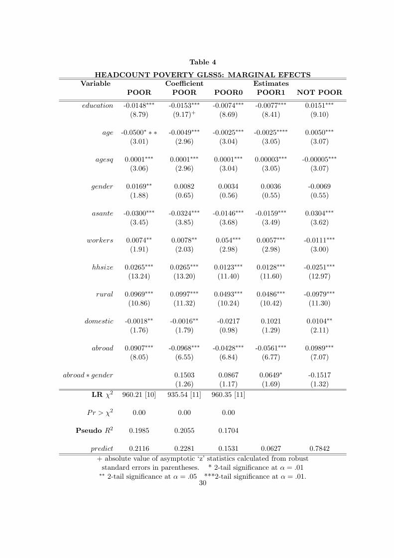
Table 4

HEADCOUNT POVERTY GLSS5: MARGINAL EFECTSVariable Coefficient Estimates

POOR POOR POOR0 POOR1 NOT POOR

education -0.0148∗∗∗ -0.0153∗∗∗ -0.0074∗∗∗ -0.0077∗∗∗ 0.0151∗∗∗

(8.79) (9.17)+ (8.69) (8.41) (9.10)

age -0.0500∗ ∗ ∗ -0.0049∗∗∗ -0.0025∗∗∗ -0.0025∗∗∗∗ 0.0050∗∗∗

(3.01) (2.96) (3.04) (3.05) (3.07)

agesq 0.0001∗∗∗ 0.0001∗∗∗ 0.0001∗∗∗ 0.00003∗∗∗ -0.00005∗∗∗

(3.06) (2.96) (3.04) (3.05) (3.07)

gender 0.0169∗∗ 0.0082 0.0034 0.0036 -0.0069(1.88) (0.65) (0.56) (0.55) (0.55)

asante -0.0300∗∗∗ -0.0324∗∗∗ -0.0146∗∗∗ -0.0159∗∗∗ 0.0304∗∗∗

(3.45) (3.85) (3.68) (3.49) (3.62)

workers 0.0074∗∗ 0.0078∗∗ 0.054∗∗∗ 0.0057∗∗∗ -0.0111∗∗∗

(1.91) (2.03) (2.98) (2.98) (3.00)

hhsize 0.0265∗∗∗ 0.0265∗∗∗ 0.0123∗∗∗ 0.0128∗∗∗ -0.0251∗∗∗

(13.24) (13.20) (11.40) (11.60) (12.97)

rural 0.0969∗∗∗ 0.0997∗∗∗ 0.0493∗∗∗ 0.0486∗∗∗ -0.0979∗∗∗

(10.86) (11.32) (10.24) (10.42) (11.30)

domestic -0.0018∗∗ -0.0016∗∗ -0.0217 0.1021 0.0104∗∗

(1.76) (1.79) (0.98) (1.29) (2.11)

abroad 0.0907∗∗∗ -0.0968∗∗∗ -0.0428∗∗∗ -0.0561∗∗∗ 0.0989∗∗∗

(8.05) (6.55) (6.84) (6.77) (7.07)

abroad ∗ gender 0.1503 0.0867 0.0649∗ -0.1517(1.26) (1.17) (1.69) (1.32)

LR χ2 960.21 [10] 935.54 [11] 960.35 [11]

Pr > χ2 0.00 0.00 0.00

Pseudo R2 0.1985 0.2055 0.1704

predict 0.2116 0.2281 0.1531 0.0627 0.7842+ absolute value of asymptotic ‘z’ statistics calculated from robust

standard errors in parentheses. * 2-tail significance at α = .01∗∗ 2-tail significance at α = .05 ***2-tail significance at α = .01.

30

Table 5

POVERTY ESTIMATES, GLSS5: OTHER MEASURES

Variable Coefficient EstimatesINCGAP INCGAPSQ EXPGAP EXPGAPSQ

education -0.4193∗∗∗ 10.9465∗∗∗ -0.2855∗∗∗ 6.5448∗∗∗

(15.50)+ (4.89) (22.75) (10.67)

age -0.1616∗∗∗ 4.9243∗ -0.0925∗∗∗∗ 0.9822∗∗

(4.39) (1.75) (5.37) (2.16)

agesq 0.0016∗∗∗ -0.0510∗ 0.0008∗∗∗ -0.0045(3.92) (1.69) (4.31) (0.65)

gender -0.5146∗∗∗ 21.0995 -0.0875 -2.2996(2.54) (1.37) (0.92) (1.02)

asante 0.3658∗ -50.2371∗∗∗ -0.1784∗ 7.3351∗

(1.73) (3.21) (1.83) (1.71)

workers -0.7313∗∗∗ 34.2735∗∗∗ 0.0806∗ -0.0204∗∗∗

(7.42) (4.56) (1.75) (1.02)

hhsize -0.3052∗∗∗ 0.5360 -0.4045∗∗∗ 4.4507∗∗∗

(6.73) (0.94) (19.08) (4.28)

rural 0.8136∗∗∗ 14.7704∗∗ 1.1868∗∗∗ -10.2293∗∗∗

(4.48) (2.09) (14.12) (2.59)

domestic -0.0019∗ -79.6120∗∗∗ 0.3177∗∗∗ 0.0014(0.09) (5.57) (3.26) (0.14)

abroad -6.1933∗∗∗ 576.6802∗∗∗ -1.1375∗∗∗ 4.2658(9.84) (28.70) (5.09) (0.47)

abroad ∗ gender -0.0041∗∗ 0.4167∗∗ -0.2161∗∗ 0.2161(2.18) (1.98) (2.89) (1.21)

Constant 4.8971∗∗∗ -215.6188∗∗ -2.5374∗∗∗ -26.9621∗∗∗

(6.17) (3.57) (5.98) (5.3467)

LR χ2 1042.56 [11] 1295.43 [11] 2420.39 [11] 1099.97 [11]Pr > χ2 0.00 0.00 0.00 0.00

Pseudo R2 0.2456 0.1789 0.456 0.1335+ absolute value of asymptotic ‘z’ statistics calculated from robust

standard errors in parentheses. * 2-tail significance at α = .01∗∗ 2-tail significance at α = .05 ***2-tail significance at α = .01.

31

Table 6

POVERTY ESTIMATES: PSEUDO-PANEL DATA

Variable Coefficient EstimatesPOOR PSTATUS INCGAP EXPGAP

education -0.0233∗∗∗ 0.0086∗∗ -0.0086∗∗ -0.0218∗∗∗

(3.33)+ (2.35) (2.29) (2.86)

age -0.5632 0.2451 -0.8075∗ -0.5065∗∗

(1.35) (1.29) (1.75) (2.09)

agesq 0.0001 0.0001 0.00005 0.0064(1.54) (1.10) (0.77) (1.02)

asante -1.9304∗∗∗ -0.1028 -0.1027 -0.3211(4.03) (0.44) (0.44) (1.06)

workers -0.0716∗∗ 0.0268∗∗ -0.0417 -0.00274∗

(2.06) (2.15) (1.01) (1.71)

hhsize 1.1821∗∗∗ -0.2011∗∗ 1.1999∗∗∗ 1.2883∗∗∗

(6.33) (2.31) (4.45) (3.28)

domestic -0.1621∗ 0.0164∗∗ -0.0013∗ -0.0022(1.82) (2.11) (1.76) (1.56)

abroad -1.0908∗∗∗ 0.4274∗∗ -1.1505∗∗∗ -0.7386∗∗∗

(2.98) (2.05) (2.77) (3.11)

abroad ∗ gender 0.0116∗∗ -0.0041∗∗ 0.0142∗∗ 0.0124∗∗

(2.09) (1.99) (2.12) (1.91)

Constant 3.2422∗∗ 1.0681∗∗ 1.8962∗∗ 1.2614(1.96) (1.99) (1.23) (2.48)

LR χ2 92.33 [9] 109.65 [9] 141 [9] 89 [9]

Pr > χ2 0.00 0.00 0.00 0.00

Pseudo R2

Hansen J 0.00 0.00 0.001 0.002

Kleinbergen-Paap LM 29.84 (0.00) 31.09 (0.00) 28.185 (0.00) 19.93 (0.00)

N 96+ absolute value of asymptotic ‘z’ statistics calculated from robust

standard errors in parentheses. * 2-tail significance at α = .01∗∗ 2-tail significance at α = .05 ***2-tail significance at α = .01.

32

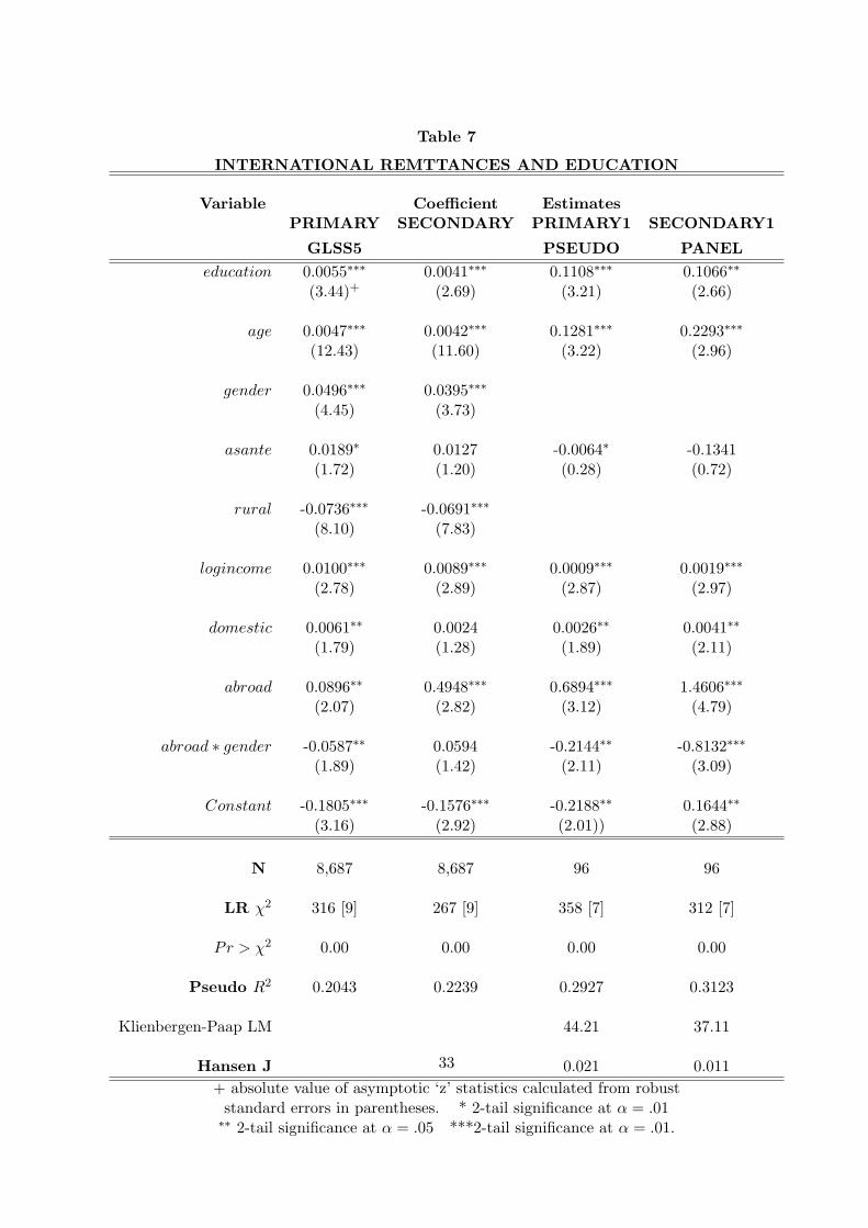
Table 7

INTERNATIONAL REMTTANCES AND EDUCATION

Variable Coefficient EstimatesPRIMARY SECONDARY PRIMARY1 SECONDARY1

GLSS5 PSEUDO PANELeducation 0.0055∗∗∗ 0.0041∗∗∗ 0.1108∗∗∗ 0.1066∗∗

(3.44)+ (2.69) (3.21) (2.66)

age 0.0047∗∗∗ 0.0042∗∗∗ 0.1281∗∗∗ 0.2293∗∗∗

(12.43) (11.60) (3.22) (2.96)

gender 0.0496∗∗∗ 0.0395∗∗∗

(4.45) (3.73)

asante 0.0189∗ 0.0127 -0.0064∗ -0.1341(1.72) (1.20) (0.28) (0.72)

rural -0.0736∗∗∗ -0.0691∗∗∗

(8.10) (7.83)

logincome 0.0100∗∗∗ 0.0089∗∗∗ 0.0009∗∗∗ 0.0019∗∗∗

(2.78) (2.89) (2.87) (2.97)

domestic 0.0061∗∗ 0.0024 0.0026∗∗ 0.0041∗∗

(1.79) (1.28) (1.89) (2.11)

abroad 0.0896∗∗ 0.4948∗∗∗ 0.6894∗∗∗ 1.4606∗∗∗

(2.07) (2.82) (3.12) (4.79)

abroad ∗ gender -0.0587∗∗ 0.0594 -0.2144∗∗ -0.8132∗∗∗

(1.89) (1.42) (2.11) (3.09)

Constant -0.1805∗∗∗ -0.1576∗∗∗ -0.2188∗∗ 0.1644∗∗

(3.16) (2.92) (2.01)) (2.88)

N 8,687 8,687 96 96

LR χ2 316 [9] 267 [9] 358 [7] 312 [7]

Pr > χ2 0.00 0.00 0.00 0.00

Pseudo R2 0.2043 0.2239 0.2927 0.3123

Klienbergen-Paap LM 44.21 37.11

Hansen J 0.021 0.011+ absolute value of asymptotic ‘z’ statistics calculated from robust

standard errors in parentheses. * 2-tail significance at α = .01∗∗ 2-tail significance at α = .05 ***2-tail significance at α = .01.

33