Religion as an Industry:Estimating a Strategic Entry Model for Churches

Michael W. Walrath∗

Department of EconomicsUniversity of St. Thomas

March 2010

Abstract

This paper treats the entry decisions of churches as if they were profit-maximizing firmsand uses recent developments in the strategic entry industrial organization literatureto study these decisions. A central theme in the entry literature is the potential forexcess entry because the entrant fails to internalize the negative impact of its entry onthe revenue of existing firms. Two key facts underlying my analysis are that Catholicchurches tend to be much bigger in terms of members than Protestant churches andthere are also fewer Catholic churches in a typical market. As compared to relativelydecentralized Protestant churches, the Catholic Church is hierarchical, with authorityfor entry decisions vested in a local bishop. One might expect the bishop to internalizenegative impact from entry of a new church, in a way that a Protestant preacher startinga new church would not. I estimate the parameters of an entry model using data fromthe entry of Protestant churches in specially defined markets and then do an experimentto determine how things look different when a Catholic bishop controls entry. I findthat I can explain a large amount of the differences in entry patterns between Catholicchurches and Protestant churches taking this difference in entry regulation into account.

JEL classification: L1,L2,Z12.

Keywords: Strategic entry, religious organizations, market structure

∗I would like to thank Thomas Holmes, Erzo Luttmer, Minjung Park, Andrew Cassey, Junichi Suzukiand the participants of the Applied Microeconomics Workshop at the University of Minnesota for commentsand suggestions. Remaining errors are mine.

Correspondence: Mail #5029, 2115 Summit Avenue, St. Paul, MN 55105; walrath@stthomas.edu

1 Introduction

Thinking about the entry process of a church, there are a number of similarities between the

decision of whether or not to open a new church and the decision of opening a new business,

such as a video store.1 The new church will incur a fixed cost, just like a video store. In order

to cover the fixed cost, the church will need revenue. A church will not generate revenue

by renting tapes, but instead by passing the collection plate. Everything else equal, a video

store’s (or church’s) revenue is more likely to cover its costs if the market population is larger

or if there are fewer rival video stores (churches) in the market. So in these respects, the

entry decision of a church is similar to the entry decision of a video store (or some other

profit-maximizing retail business).

In the past 20 years much work has been done in the IO literature concerning the strategic

entry of retail firms.2 One of the seminal papers in the entry literature is Bresnahan and

Reiss (1991). They estimate a model of entry for dentists, plumbers, tire dealers, etc. in

small, rural markets. There have been many methodological contributions in recent years.

Seim (2001) studies video stores, Aguirregabiria and Mira (2007) study restaurants, gas

stations, bookstores, etc. Though the methodologies used differ, a common thread to this

work is that entry of a firm depends on market size and the firm’s expectations about the

number of rival firms. Also, in these models there is “excess entry” from the perspective of

the firm. An entering firm does not take into account the negative effect of its entry on the

revenue of other firms in the market.

This paper applies empirical methods that have been developed to study entry of re-

tail firms to the entry of churches. I find that these methods are successful in explaining

the difference in entry between Catholic and Protestant churches (section 2 discusses these

1The distinction between a “small ‘c’ church,” which is a building for worship, and “large ‘C’ Church”which refers to a religion is important. I am focusing on the creation of churches in different markets, whichcan be thought of as plant level, not firm level.

2See Berry and Reiss (2007) for a discussion of this literature.

1

different religious groupings). Compared to Catholics, Protestant churches seem to satisfy

the standard “free-entry” condition. There is no central authority regulating the entry of

Protestant churches. However, Catholics have a strict hierarchy going from priest to bishop

to pope (with a number of steps between); through this hierarchy Catholics regulate entry.3

I use methods of estimating entry games to show that the regulation of entry can explain

why in a typical market there are fewer Catholic churches than Protestant churches.

The particulars of what I do follow. As in Bresnahan and Reiss (1991), I study entry in

small, rural markets. I take advantage of advances in Geographic Information Systems (GIS)

technology, so I can be more careful in my definition of markets. My methodological approach

draws on various aspects of Bresnahan and Reiss (1991), Seim (2001) and Aguirregabiria and

Mira (2007). First, I estimate the structural parameters of an entry game (such as fixed costs,

etc.) using only the entry behavior of Protestants. Second, I study the entry decisions of

Catholic churches using the structural parameters from the Protestant estimation and feeding

in Catholic demographics. If I assume Catholic churches engage in unregulated entry, I find

that Catholic entry behavior looks much like Protestant entry behavior (number of churches

in a given market). However, when I use Protestant parameters, Catholic demographics and

assume that Catholic entry is being regulated by a planner (bishop), there is substantially

less entry. I find that this difference in entry regulation accounts for essentially all of the

difference in entry behavior observed in the data.

This paper specifically addresses the question: if Catholics were just like Protestants

except for demographics and the presence of a Catholic planner, what would be the difference

in entry behavior? There could be a number of other possible explanations for the difference

in church entry behavior that this paper does not account for. In the conclusion I discuss

a few possible alternative explanations that may also play a role. Taking these alternatives

into account now would add substantial complications. To make progress, in this paper I

3See Mitchell (2007) and Takayama (1975) for a discussion of differences in organizational structurebetween different denominations.

2

focus on how far I can get explaining the difference in entry behavior just taking into account

demographics and difference in entry regulation. I find that these two factors go quite far in

explaining the difference in entry behavior.

This paper contributes to two different literatures. One is the literature on free entry and

regulation. In perfectly competitive markets entry regulation is thought to be detrimental.

However, Mankiw and Whinston (1986) show theoretically that in an oligopoly market it

is possible for free entry to result in excess entry. Berry and Waldfogel (1999) and Hsieh

and Moretti (2003) empirically study welfare loss of free-entry. My paper does not model

consumers, so I cannot make any statements about total welfare. (Given the topic, it could

be quite dangerous to discuss the welfare of consumers.) I only focus on excess entry from

the perspective of the church.

This paper also adds to the economics of religion literature. The notion of a market

for religion was alluded to as long ago as Adam Smith’s Wealth of Nations. He discusses

the difference between clergy who “depend [. . . ] upon the voluntary contributions of their

hearers” and clergy who depend on “some other fund to which the law of their country

may entitle them” (Smith (1776), 486). He says that government subsidized clergy fall

behind in “Their exertion, their zeal and industry” compared to clergy not dependent on

the government (Smith (1776), 486). Iannaccone (1998) reviews the work that has been

done applying economic concepts to religion in the past 30 years. Much work has focused

on individual’s decisions regarding religious attendance.4 There has also been work relating

religious participation to various outcomes, such as educational attainment and income (for

example, Gruber (2005)). There has been limited work treating churches as firms. For

example Ekelund (1996) treats the Medieval Catholic Church as a monopolist. This paper

4For example, Azzi and Ehrenberg (1975) study the decision of church attendance by treating it as ahousehold utility maximization problem (with consumption of both corporeal and after-life goods) subjectto a time constraint.

3

is the first to treat the creation of a new church as a result of strategic entry decision.5

The paper proceeds as follows. Section 2 provides some background on thinking of

religion as an industry; section 3 presents a simple theoretical model of church entry; section

4 presents the empirical model; section 5 discusses the estimation strategy; section 6 describes

the data; section 7 looks at descriptive evidence; section 8 presents the results of the entry

game and then looks at the effect of a Catholic planner and section 9 concludes.

2 Background on Religion as an Industry

This section deals with some particular characteristics of religion in the US that will inform

modeling choices made in the paper. First I will discuss common groupings of religions used

in the study of religion. Then I will discuss differences in organizational structure and the

decision of starting a new church in different religious groups. Then I will give examples of

fixed costs of starting a church and discuss the assumption of profit-maximization.

This paper will specifically deal with Christian religions. More specifically, Catholic and

Protestant denominations. I will consider three separate religious groups. These groupings

are given in table 1 and are based on classifications in Pew (2008) and Ammerman (2001).6

The group Catholics are made up solely of the Roman Catholic Church. Within each broad

classification of Protestantism there are a number of denominational families. For example

Mainline Protestants are made up of the denominational families Lutheran, Methodist, Con-

gregational, etc. Some of these denominational families are made up of a number of separate

denominations. For example, different denominations contained within the denominational

family of Lutheran include the Evangelical Lutheran Church of America (ELCA), Lutheran

5The distinction between, church and Church is important; Montgomery (1996) has a theoretical ap-proach to the creation of new religions.

6The classifications in these two sources have some differences so my categories synthesize the categoriesin these two sources. Pew (2008) places American Baptist Churches into the Mainline Protestants, whileother Baptist denominations are Evangelical Protestants. Due to limitations on the data, for this paper allBaptist denominations are counted as Evangelical Protestant.

4

Table 1. Makeup of Religious Groups

Religious Group Denominational Family

Catholic Roman Catholic ChurchMainline MethodistProtestant Lutheran

PresbyterianAnglicanCongregational

Evangelical BaptistProtestant Holiness

RestorationistPietiestsReformedPentecostalAdventistAnabaptist

Church - Missouri Synod, Lutheran Church - Wisconsin Synod. Individuals switch between

all of these three groups, but switching between a Protestant denomination and Catholicism

is less likely than switching between different Protestant denominations. (This is supported

by Pew (2008) and Loveland (2003).)

Since the Protestant groups are made up of a number of different denominations, each

Protestant group will have less centralized control than the Catholics, which is comprised of

just the Roman Catholic Church. Also, the Roman Catholic Church has a particularly strict

hierarchical structure. In general each Protestant denomination will have a less centralized

organizational structure. 7

Some anecdotal evidence of differences in organizational structure can be seen when

looking at the process of opening a new church. From the Vatican website, the Directory for

7From Takayama (1975):

For the most part Protestants deplore the legality, hierarchy, and tradition which are found inthe organizational structure of the Roman Catholic Church. They believe that their organiza-tions can operate effectively without recourse to a well-defined line of authority.

5

the Pastoral Ministry of Bishops specifically details the “Planning for the Establishment of

Parishes.”

[. . . ]the Bishop should proceed, after consulting the diocesan presbyteral council

(660), to alter territorial boundaries, to divide parishes that are too large, to

merge small parishes, to establish new parishes [. . . ] [anyone who] wish[es] to

build churches within the territory of the diocese, they must first obtain written

permission from the Bishop.

This clearly states the Bishop’s responsibility for and control over planning new churches in

his diocese (specific geographical region). This formal statement of policy is in stark contrast

to the more eager discussion of “church planting” (the common phrase used for creating a

new church) by different Protestant denominations. For example the Episcopal Church in the

USA has a number of pages regarding church planting. They detail the necessary steps of the

process, including “Demographic study is done before site selection” and “Other Christian

communities identified.”8 Both the United Church of Christ and the United Methodists have

had conferences at which Reverend Jim Griffith, president of Griffith Coaching Network has

discussed planting.9 These differences between Catholics and Protestant groups motivate

modeling decisions made later in the paper regarding whether entry by a religious group is

centrally or de-centrally planned.

In the model presented later there are variable profits, that depend on the size of the

market and there will be a fixed cost for each church. Stonebraker (1993) discusses church

costs:

As the number of members goes up, the average cost of servicing each mem-

ber goes down. Attendance at liturgies, Sunday School classes, youth groups,

8http://www.episcopalchurch.org/newchurch_4321_ENG_HTM.htm?menu=undefined accessed Octo-ber 19, 2008

9Information found at http://www.secucc.org/development/leadtrain2.php and http://www.

nccumc.org/docs/leadershipacademy/jgriffithbio.pdf on October 19, 2008.

6

and Bible studies rarely approaches physical capacity. Empty pews abound and

additional participants can be served at little or no extra cost.

A necessary component of a church is a clergy member. Required training for clergy can be

thought of as a fixed cost of a new church. According to Lipford (1992), “the processes by

which clergy qualify for employment is [. . . ] strictly regulated in most denominations.” Re-

quirements do vary across denominations. For example, clergy in denominations such as the

Roman Catholic Church, the United Methodist church and the Episcopal Church in the USA,

“are subject to rigorous monitoring, examinations, and educational requirements” (Lipford

(1992)). However, for clergy from the Southern Baptist Convention, though they often “at-

tend seminaries that are supported by the denomination, the SBC sets no requirements for

ministers serving in its denomination” (Lipford (1992)).

As mentioned above, the entrance of a new church incurs a fixed cost (the building itself,

certain services, the necessary clergy). A church also earns revenues. This paper assumes

that a potential entering church must expect revenues to be greater than costs. The clergy

member starting this new church has an opportunity cost, if revenues do not cover costs, the

clergy will do something else. Below I consider expected profit for a church and will impose

a zero-profit condition.

3 Theory

This section first presents a simple theoretical model of the market for religion. Then I discuss

some analytical results. This section concludes with a discussion of how the empirical model

used later in the paper differs from the theoretical model.

The model presented in this section is very similar to the model in Anderson and

De Palma (1992). First consider a logit-style demand framework. Individual i has util-

7

ity for church j given by:

uij = a− pj + µξij (1)

Where a is some constant, pj is the price of attending church j, ξij is a utility shock dis-

tributed by a type-1 extreme value distribution and µ represents the level of product differ-

entiation. The probability that individual i will attend church j will be:

Pij =exp[(a− pj)/µ]∑N

k=1 exp[(a− pk)/µ] + exp[V0/µ](2)

V0 is the deterministic utility of the outside option, which in this case would be non-

attendance. If there were no outside good, (V0 → −∞), it would imply that all people

attend some church. If a market has population S, then church j will have attendance PijS.

Now consider the supply side. There are a certain number of religious entrepreneurs who

can potentially enter (create a church). An entrant incurs fixed cost γ. As mentioned above

there is some price, pj, of attending a church. Church j will earn revenues, pjPijS (price

times number of attendees).

In general a church does not set a price of admission and collect it at the door. Individuals

choose the amount they place in a collection plate. Consumers choosing their own price

eliminates price competition. The price of every church would be the same p (one can

think of p as the average contribution of all church-goers). The number of churches that

will enter, N , will depend on structure of the market. I will consider two different market

structures. One structure will be free-entry by religious entrepreneurs, the other will be a

single monopoly religion with the number of churches determined by a planner. As expected,

the number of churches in a market is larger if there is free entry than if there is a planner.

Proposition 3.1. With consumer utility given in equation (1) and fixed price p for every

church, the number of churches in market with free-entry, NF , will be greater than or equal

to the number of churches chosen by a planner, NP .

8

Proof. See appendix.

The key difference between free-entry and a planner is that in free-entry each potential

entrant only cares about the profit it earns. Entry will occur until per church profits are

driven to zero. When a planner makes a decision to add a church, it takes into account the

profits of that church but also the negative effect on the other churches in the market. If

everyone attended a church, (V0 → −∞), the number of customers per church would be SN

.

In this case a planner would either choose zero churches (if pS < γ) or just one church (if

pS ≥ γ). With revenues being evenly split and each additional church incurring a fixed cost,

a planner would never place more than one church in a market.

When everyone attends a church (no outside good) the effect of changes in fixed price, p,

level of product differentiation, µ, market size, S, and fixed cost, γ, on number of churches

that will enter in free-entry, NF , is immediate.10 In this case the pool of church revenue, pS

is split evenly among the N churches in a market such that each church earns revenue pSN

.

With no outside good, the number of people who go to church is fixed, so as the fixed price,

p, increases, the pool of possible revenues increase. So in free-entry the number of churches

will increase. With no outside good and no price competition, product differentiation, µ,

will have no effect. The number of churches will grow proportionately with market size, S.

The number of churches would be inversely proportional to the fixed cost, γ.

If there is an outside good these effects can be less clear.11 With an outside good the

effect of changing the price level, p, has two effects. It increases the price each church-goer

pays, but causes more people to choose the outside good. For small p as the price increases

at first revenues will increase and then eventually start to decrease. When the total revenue

increases, the number of churches that will enter will increase; as revenues decrease the

number of churches that enter will decrease. The effect of a change in the level of product

10Under these conditions, profit per church, if there are N churches is given by: ΠN = pSN − γ

11Now per church profits, if there are N churches, is given by: ΠN = pSN+exp[(V0−a+p)/µ] − γ.

9

differentiation, µ, depends on the value of the outside good. If V0 − a + p < 0, then an

increase in µ decreases revenue, thus decreasing the number of churches that will enter. On

the other hand, if V0− a+ p > 0 then an increase in product differentiation, µ, will increase

per church revenue, causing more churches to enter. Increasing market size, S, will cause

more churches to enter, but the increase in churches will not be proportional to market size.

Increasing fixed cost, γ, will decrease the number of churches, but the decrease will not be

proportional.

One way to interpret more than one religious group in a certain market is to think of

products j = 1, . . . , N as churches of a specific religious group, while V0 represents utility

from all other religious groups (“no religion” would be one of these other groups). A change

such as lower p or higher µ would increase the number of people attending a church in the

given religion and decrease the number of people attending churches of other religions.

The model described below abstracts away from the above demand framework. A number

of religious groups will be considered. There is no data on price to generate revenue similar

to above. Instead there will be a reduced form per capita variable profit function that uses

demographic data for each market. This per capita profit will be multiplied by market

population. Instead of per capita profit being split among N churches as an explicit function

of N , I allow profits to decline at different rates as N increases.

4 Empirical Model

I want to take some aspects of the simple theoretical model above and apply it to data. In

this section I discuss the empirical model I use and the equilibrium concept I apply. For

the empirical model I abstract away from the demand side and use a reduced form profit

equation (similar to that seen in Bresnahan and Reiss (1991)). There are m = 1, . . . ,M

markets. Within each market each religious type has a number of potential entrants (religious

entrepreneurs), Nmaxr , which is finite. I allow for different religious groups, r ∈ R (details and

10

reasoning discussed in section 2). Religious entrepreneurs within a certain religious group

share a common cost shock and engage in free-entry.12 Within a religious group the religious

entrepreneurs have full information, they know what the other entrepreneurs of the same

type will do. This full information structure with free-entry is similar to Bresnahan and

Reiss (1991). While there is full information within a religious type, there will be incomplete

information across religious types. For example, a Mainline Protestant entrepreneur does

not know the Evangelical Protestant specific cost shock. Across religious groups an imperfect

information game is played (much like Seim (2001)).

4.1 Profit

For a specific market there are per-capita variable profits that depend on demographic char-

acteristics, X, the number of churches of the same religious type, Nr, and the number of

churches of other religious types N−r. The parameters multiplying demographic variables,

βr and δr are religious-type specific. The number of churches of other religious types, Nq

for q 6= r, is multiplied by θr,q. θr,q is the competitive effect of each church of type q on a

church of type r, it is not symmetric (θr,q 6= θqr necessarily). If churches of different religious

types are competing with each other (if one church can steal members from churches of other

types) then θr,q will be negative. One specific demographic characteristic is Fr, the fraction

of people in the market that are of religious type r. Explicitly, per-capita variable profit is

given by:

Vr(N−r, X, Fr) = δrFr +Xβr + α1r −

∑q 6=r

θr,qNq (3)

12An example of a religious group specific cost shock could be that perhaps Mainline Protestants in acertain market require an unusually high level of family services.

11

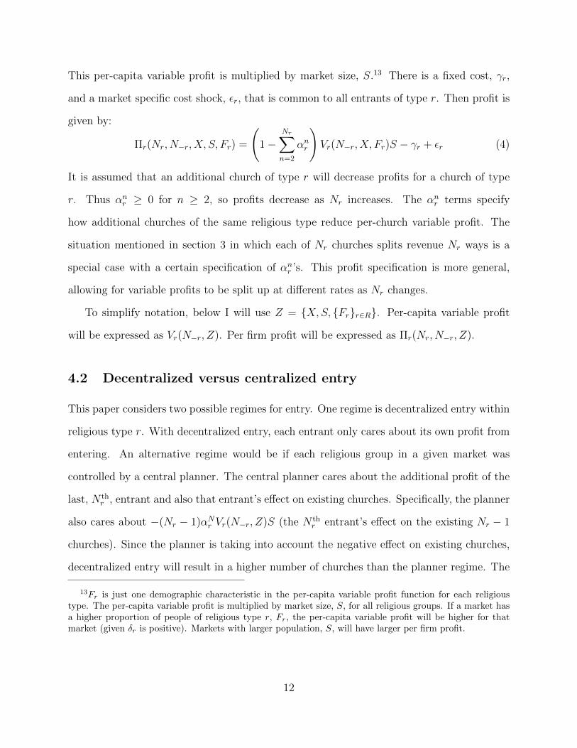
This per-capita variable profit is multiplied by market size, S.13 There is a fixed cost, γr,

and a market specific cost shock, εr, that is common to all entrants of type r. Then profit is

given by:

Πr(Nr, N−r, X, S, Fr) =

(1−

Nr∑n=2

αnr

)Vr(N−r, X, Fr)S − γr + εr (4)

It is assumed that an additional church of type r will decrease profits for a church of type

r. Thus αnr ≥ 0 for n ≥ 2, so profits decrease as Nr increases. The αn

r terms specify

how additional churches of the same religious type reduce per-church variable profit. The

situation mentioned in section 3 in which each of Nr churches splits revenue Nr ways is a

special case with a certain specification of αnr ’s. This profit specification is more general,

allowing for variable profits to be split up at different rates as Nr changes.

To simplify notation, below I will use Z = X,S, Frr∈R. Per-capita variable profit

will be expressed as Vr(N−r, Z). Per firm profit will be expressed as Πr(Nr, N−r, Z).

4.2 Decentralized versus centralized entry

This paper considers two possible regimes for entry. One regime is decentralized entry within

religious type r. With decentralized entry, each entrant only cares about its own profit from

entering. An alternative regime would be if each religious group in a given market was

controlled by a central planner. The central planner cares about the additional profit of the

last, N thr , entrant and also that entrant’s effect on existing churches. Specifically, the planner

also cares about −(Nr − 1)αNr Vr(N−r, Z)S (the N th

r entrant’s effect on the existing Nr − 1

churches). Since the planner is taking into account the negative effect on existing churches,

decentralized entry will result in a higher number of churches than the planner regime. The

13Fr is just one demographic characteristic in the per-capita variable profit function for each religioustype. The per-capita variable profit is multiplied by market size, S, for all religious groups. If a market hasa higher proportion of people of religious type r, Fr, the per-capita variable profit will be higher for thatmarket (given δr is positive). Markets with larger population, S, will have larger per firm profit.

12

difference between these two regimes can be internalized. Consider the profit function:

Πr(Nr, N−r, Z;λr) = Πr(Nr, N−r, Z)− λr(Nr − 1)αnrVr(N−r, Z)S (5)

Where Πr(Nr, N−r, Z) is defined in equation (4). If λr = 0 then the above represents the

profit for the N thr religious entrepreneur engaged in free entry. If λr = 1 then the above

represents profit of the N thr church if religion r is being run by a planner. Πr(Nr, N−r, Z)

gives the marginal profit of the N thr entrant. Internalizing the presence of a central planner

allows me to impose a zero-profit free entry condition whether or not there is centralized or

decentralized entry. There will be Nr churches of type r in a market if the expected profit

of the N thr church is positive and the expected profit of the (Nr + 1)th church is negative.

4.3 Equilibrium

Within each religious type all potential entrants know the εr draw for that religion. However,

potential entrants within religion r do not know εq for religions q 6= r. Thus there is

an incomplete information game. For the private information game between religions we

will treat each religious group as a single player no matter if entry within each religion is

decentralized or determined by a planner. Similar to Bresnahan and Reiss (1991), at the

level of a religious group I am only interested in the number of churches in a market, Nr. I

am not interested in the identity of the churches.

Each religious type, r, has beliefs about the actions of other religious types (number of

churches of another religious type that will enter a certain market) that are a function of

market characteristics; these beliefs are denoted by σ−r(·|Z), where Z = X,S, Frr∈R.

Define a strategy function sr(Z, εr, σ−r(·|Z)), that maps market characteristics, error terms

and religious group r’s beliefs about rival religious groups into a number of churches of type

r, Nr. In a Bayesian-Nash equilibrium each religion behaves optimally conditional on its

13

beliefs being correct.

Each religion has expected profits given by:

πr(Nr, Z, εr;λr, σ−r(·|Z)) =∑N−r

Πr(Nr, N−r, Z, εr;λr)σ−r(N−r|Z)

At the level of a religious type there will be free entry. There will be a number of churches

Nr such that expected profit for each of the Nr churches is positive, but per church expected

profit is negative if there are Nr + 1 churches. This is just like the zero-profit condition used

in Bresnahan and Reiss (1991), except expected profits are being used since each religious

type is now playing a game of incomplete information with other religious types.

For the game described above we can define a Bayesian-Nash equilibrium:

Definitions. A Bayesian-Nash equilibrium for this game is:

1. a set of strategies, s∗r(Z, εr, σ∗−r(·|Z))

2. beliefs on rival religions σ∗−r(·|Z)

for r ∈ R, such that:

πr(s∗r(Z, εr, σ

∗−r(·|Z)), Z, εr;λr, σ

∗−r(·|Z)) ≥ 0 and

πr(s∗r(Z, εr, σ

∗−r(·|Z)) + 1, Z, εr;λr, σ

∗−r(·|Z)) < 0

and

σ∗r(Nr|Z) = Pr[πr(Nr, Z, εr;λr, σ

∗−r(·|Z)) ≥ 0 and

πr(Nr + 1, Z, εr;λr, σ∗−r(·|Z)) < 0

]where

σ∗−r(N−r|Z) =∏q 6=r

σ∗q (N−r(q)|Z)

14

5 Estimation Strategy

In order to estimate this game I will use the Nested Pseudo Likelihood (NPL) algorithm of

Aguirregabiria and Mira (2007), applied to a static game. The general idea is to take a set of

beliefs as given. Given these beliefs estimate parameters by maximizing a pseudo likelihood

(it is a pseudo likelihood since the true beliefs are not being used). Using the parameter

estimates, update the beliefs. This process is repeated until the sets of beliefs converge. One

advantage of this method is that it is computationally light; it does not require solving for

a fixed point for each set of parameters. Also, in games of incomplete information multiple

equilibria are possible. This technique automatically selects the equilibrium that fits the

data.

Let the set of parameters to be estimated be denoted by ω = δr, αrn

Nrmax

n=1 , θr,qq 6=r, γrr∈R.

Data on observed church counts are given by Nr,m for r ∈ R and m = 1, . . . ,M .

The algorithm is as follows:

1. At iteration n take set of beliefs σ(n). For n = 1 use arbitrary initial guess.

2. Given beliefs σ(n) construct a pseudo likelihood function L(ω, σ(n)) and obtain the

pseudo maximum likelihood estimator of ω as ω(n) = arg maxω∈Ω L(ω, σ(n)) (this like-

lihood is defined below).

3. Update beliefs using the probability mapping, σ(n+1)(Nr,m) = Ψ(Nr,m|Z, λ, ω(n), σ(n))

(this mapping is defined below).

4. If ‖σ(n+1) − σ(n)‖ is smaller than some set number, then choose ω(n+1), σ(n+1) as the

NPL estimator. Otherwise, repeat above steps using σ(n+1) as a new guess.

Assuming the religious type specific shock, εr, is drawn from a standard normal distri-

bution, the likelihood function will be an ordered probit.

15

As said above, at the level of religious group r, the number of churches in a given market

must satisfy a free entry condition. Denote the deterministic portion of expected profit by

Πr(Nr, Z;λr, σ−r(·|Z))) = πr(Nr, Z, εr;λr, σ−r(·|Z))− εr. The CDF for the standard normal

distribution is denoted by Φ(·).

There will be zero churches if πr(1, Z, εr;λr, σ−r(·|Z)) < 0. The probability of zero

churches is given by:

Pr(Nr = 0) = Pr(εr < −Πr(1, Z;σ−r(·|Z))) = Φ(Πr(1, Z;λr, σ−r(·|Z))) (6)

There will beN churches if πr(N,Z, εr;λr, σ−r(·|Z)) ≥ 0 and πr(N+1, Z, εr;λr, σ−r(·|Z)) < 0.

The probability of there being N churches is given by:

Pr(Nr = N) = Pr(εr ≥ −Πr(N,Z;λr, σ−r(·|Z)) and εr < −Πr(N + 1, Z;λr, σ−r(·|Z))

)= Φ

(−Πr(N + 1, Z;λr, σ−r(·|Z))

)− Φ

(−Πr(N,Z;λr, σ−r(·|Z))

)(7)

Let Nmaxr be the maximum possible number of churches of type r in one market. There will

be Nmaxr churches if πr(N

maxr , Z, εr;λr, σ−r(·|Z)) > 0. The probability of there being Nmax

r

churches is given by:

Pr(Nr = Nmaxr ) = Pr(εr ≥ −Πr(N

maxr , Z;λr, σ−r(·|Z)))

= 1− Φ(Πr(N

maxr , Z;λr, σ−r(·|Z))

) (8)

16

Then the probability mapping, Ψ(ω(n), σ(n)), mentioned in the above algorithm can be

expressed as:

Ψ(Nr|Z, λ, ω(n), σ(n)) =

Φ(Πr(1, Z;λr, σ(n)−r )) if Nr = 1,

Φ(−Πr(Nr + 1, Z|λr, σ(n)

−r ))

−Φ(−Πr(Nr, Z|λr, σ(n)

−r ))

if 1 < Nr < Nmaxr ,

1− Φ(Πr(Nmaxr , Z|λr, σ(n)

−r ) if Nr = Nmaxr

(9)

Given Ψ(ω(n), σ(n)), the likelihood L(ω, σ(n)):

L(ω, σ(n)) =M∑

m=1

∑r∈R

Nmaxr∑

N=1

1Nr,m = Nr ln(Ψ(Nr|ω(n), σ(n))

)

Where Nr,m are the observed church counts from the data.

6 Data

In order to estimate the above model I need data on church counts and market characteristics

for a specific set of markets. Instead of taking market definitions from the Census, I will

create my own definition of a market.

6.1 Defining markets

I will focus on small, isolated, rural markets. There is much religious activity in small

towns. Bresnahan and Reiss (1991) use isolated markets as their unit of analysis since it is

more likely that the market population is consuming goods within that market. Pre-defined

17

Census markets include Metropolitan Statistical Areas (MSA’s) and Census Places. Since

religious activity occurs at a very local level, MSA’s are far too large. Bresnahan and Reiss

(1991) specifically use Census places that meet specific isolation criteria. As Holmes and

Lee (2007) describe, designation as a Census place is often arbitrary. Census Places leave

out 25% of the US population. Instead of only considering clusters of population that the

Census decides are markets, I want to look at all clusters of population and decide whether

or not each one constitutes a market. I start with Census blocks (the finest level at which

Census data is reported) and aggregate to create a market. Once my markets are created I

then impose isolation criteria.

Since the ultimate goal is a set of isolated markets I begin by taking all Census blocks in

the lower 48 states and the District of Columbia, that are not in a Metropolitan Statistical

Area (MSA). This leaves me with 3,877,307 out of 8,164,718 Census blocks. The general idea

is to find a set of population clusters that are some minimum distance from each other. I

treat each non-MSA block as a potential “center.” I find a set of “centers” that meet certain

criteria regarding distance from other “centers.” A market is defined to be everything within

3 miles of these selected centers. (See Appendix B.1 for more detail.) There are 5,586 markets

that meet my criteria. Market populations are determined by summing up the population

of all Census blocks within 3 miles of a market’s center. These markets have uniform area,

unlike Census Places which vary in area.

I start with these 5,586 markets and then, following Bresnahan and Reiss (1991), I impose

additional isolation criteria.14,15 Specifically, the population within 10 miles of the market

must be less than 10,000, the population within 20 miles must be less than 30,000, and the

14The 5,586 markets already have some isolation imposed on them through the process by which theywere created (since potential markets come from non-MSA’s and need to be a certain distance from eachother)

15The isolation criteria in this paper are based on total population within a certain radius of a potentialmarket. Whereas in Bresnahan and Reiss (1991), the isolation criteria are based on the proximity of otherCensus places with certain populations.

18

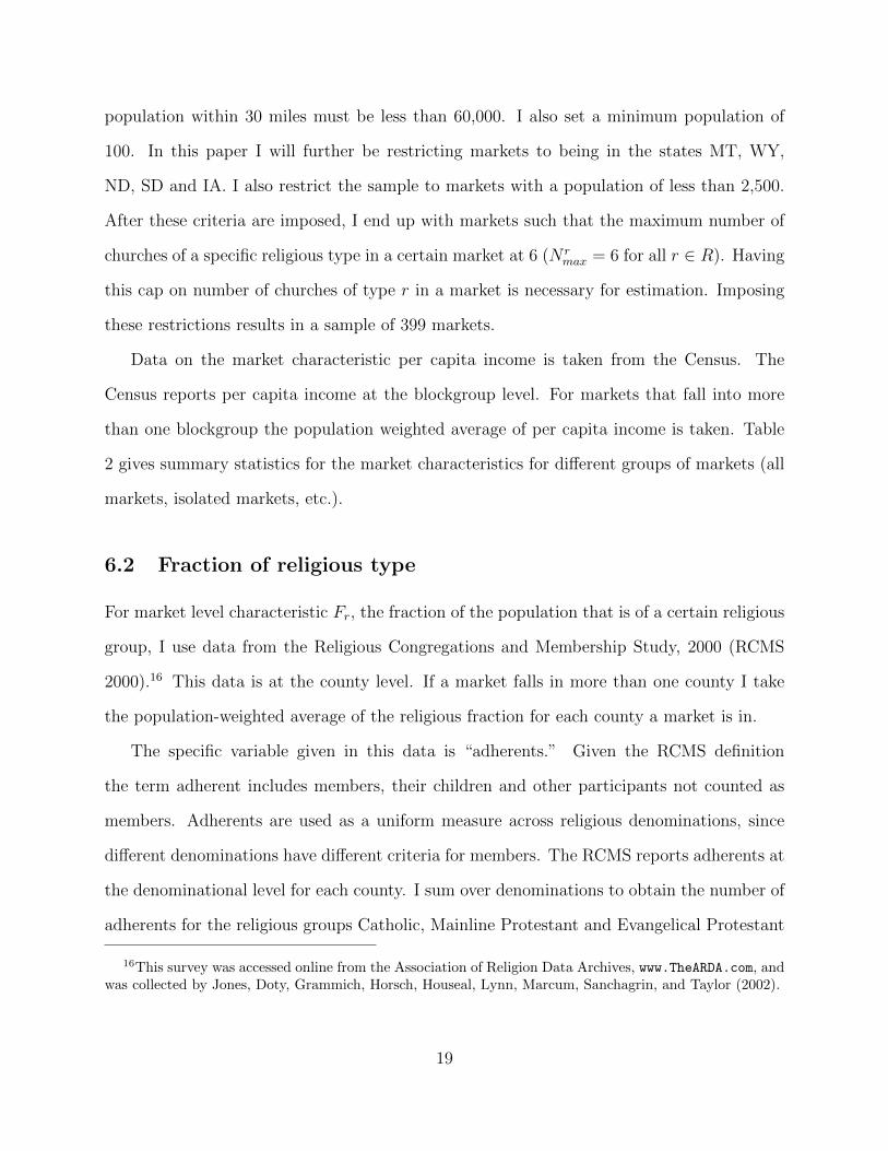
population within 30 miles must be less than 60,000. I also set a minimum population of

100. In this paper I will further be restricting markets to being in the states MT, WY,

ND, SD and IA. I also restrict the sample to markets with a population of less than 2,500.

After these criteria are imposed, I end up with markets such that the maximum number of

churches of a specific religious type in a certain market at 6 (N rmax = 6 for all r ∈ R). Having

this cap on number of churches of type r in a market is necessary for estimation. Imposing

these restrictions results in a sample of 399 markets.

Data on the market characteristic per capita income is taken from the Census. The

Census reports per capita income at the blockgroup level. For markets that fall into more

than one blockgroup the population weighted average of per capita income is taken. Table

2 gives summary statistics for the market characteristics for different groups of markets (all

markets, isolated markets, etc.).

6.2 Fraction of religious type

For market level characteristic Fr, the fraction of the population that is of a certain religious

group, I use data from the Religious Congregations and Membership Study, 2000 (RCMS

2000).16 This data is at the county level. If a market falls in more than one county I take

the population-weighted average of the religious fraction for each county a market is in.

The specific variable given in this data is “adherents.” Given the RCMS definition

the term adherent includes members, their children and other participants not counted as

members. Adherents are used as a uniform measure across religious denominations, since

different denominations have different criteria for members. The RCMS reports adherents at

the denominational level for each county. I sum over denominations to obtain the number of

adherents for the religious groups Catholic, Mainline Protestant and Evangelical Protestant

16This survey was accessed online from the Association of Religion Data Archives, www.TheARDA.com, andwas collected by Jones, Doty, Grammich, Horsch, Houseal, Lynn, Marcum, Sanchagrin, and Taylor (2002).

19

(using the classification given in table 1). Since this is county level data, and each market

should be a fairly small portion of any county, I consider this fraction to be the average

religious tendency of the market.

6.3 Church counts

Data on the number of churches in each of these markets have been collected. Due to data

collection limitations, this paper will focus on the states of MT, WY, ND, SD and IA.

Specifically, the data pertains to markets that are completely contained within these five

states.

For each market I need a count of churches. To collect these counts I use two different

sources. One is an online directory (a phone book), ReferenceUSA. The other is specifically

an online directory for Catholic Churches, http://parishesonline.com.

I select all churches from ReferenceUSA (using NAICS=8131008) and all Catholic churches

from parishesonline.com that are in the above mentioned states. I have longitude and lat-

itude for each church. Any church that is within 3 miles of the above described “centers”

is in that specific market. Churches from ReferenceUSA are classified as being Mainline or

Evangelical Protestant. Church counts for different groups of markets can be seen in Tables

6 and 7.

20

Table 2. Summary Statistics for Market Characteristics

Market Number StandardCategory Markets Minimum Maximum Mean DeviationAll MarketsPopulation (in thousands) 5586 0.001 53.687 4.171 6.671Per Capita Income (in thousands) 5586 0.000 44.721 16.043 3.808Share Catholic 5586 0.000 0.947 0.163 0.159Share Mainline Protestant 5586 0.000 0.932 0.150 0.142Share Evangelical Protestant 5586 0.000 1.107 0.184 0.174Isolated MarketsPopulation (in thousands) 1857 0.100 44.874 2.512 4.107Per Capita Income (in thousands) 1857 3.649 44.720 15.529 3.867Share Catholic 1857 0.000 0.947 0.198 0.163Share Mainline Protestant 1857 0.000 0.932 0.183 0.172Share Evangelical Protestant 1857 0.000 0.989 0.156 0.171Isolated Markets in Select StatesPopulation (in thousands) 483 0.100 28.735 2.013 3.771Per Capita Income (in thousands) 483 3.649 35.085 15.602 3.885Share Catholic 483 0.006 0.869 0.235 0.154Share Mainline Protestant 483 0.026 0.882 0.303 0.194Share Evangelical Protestant 483 0.000 0.576 0.081 0.054Selected MarketsPopulation (in thousands) 399 0.100 2.475 0.726 0.616Per Capita Income (in thousands) 399 3.649 35.085 15.412 4.043Share Catholic 399 0.006 0.869 0.237 0.156Share Mainline Protestant 399 0.026 0.882 0.313 0.197Share Evangelical Protestant 399 0.000 0.576 0.081 0.057

Note: the religious shares come from the RCMS, which says that it is possible for shares to be larger than 1(i.e. 1.107) due to people living in areas surrounding a county attending a church within that county.

21

7 Descriptive Evidence

Before estimating the model, I look at the relationship between population and church counts.

First, to look at the entire US, I will use the RCMS data mentioned above. The finest level

at which this data is available is county-level. For this analysis I will consider a county to be

a market. Using the RCMS data, in the year 2000, in total there were 266,459 congregations

(churches) with 140,718,046 adherents in the contiguous 48 states and Washington DC (these

numbers include all religions).17

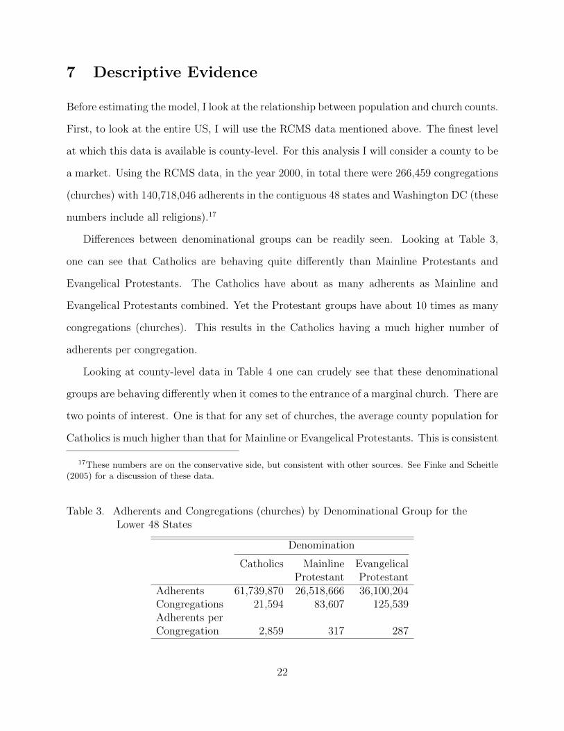
Differences between denominational groups can be readily seen. Looking at Table 3,

one can see that Catholics are behaving quite differently than Mainline Protestants and

Evangelical Protestants. The Catholics have about as many adherents as Mainline and

Evangelical Protestants combined. Yet the Protestant groups have about 10 times as many

congregations (churches). This results in the Catholics having a much higher number of

adherents per congregation.

Looking at county-level data in Table 4 one can crudely see that these denominational

groups are behaving differently when it comes to the entrance of a marginal church. There are

two points of interest. One is that for any set of churches, the average county population for

Catholics is much higher than that for Mainline or Evangelical Protestants. This is consistent

17These numbers are on the conservative side, but consistent with other sources. See Finke and Scheitle(2005) for a discussion of these data.

Table 3. Adherents and Congregations (churches) by Denominational Group for theLower 48 States

Denomination

Catholics Mainline EvangelicalProtestant Protestant

Adherents 61,739,870 26,518,666 36,100,204Congregations 21,594 83,607 125,539Adherents perCongregation 2,859 317 287

22

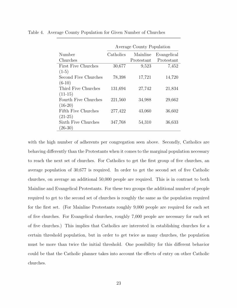
Table 4. Average County Population for Given Number of Churches

Average County Population

Number Catholics Mainline EvangelicalChurches Protestant ProtestantFirst Five Churches 30,677 9,523 7,452(1-5)Second Five Churches 78,398 17,721 14,720(6-10)Third Five Churches 131,694 27,742 21,834(11-15)Fourth Five Churches 221,560 34,988 29,662(16-20)Fifth Five Churches 277,422 43,060 36,602(21-25)Sixth Five Churches 347,768 54,310 36,633(26-30)

with the high number of adherents per congregation seen above. Secondly, Catholics are

behaving differently than the Protestants when it comes to the marginal population necessary

to reach the next set of churches. For Catholics to get the first group of five churches, an

average population of 30,677 is required. In order to get the second set of five Catholic

churches, on average an additional 50,000 people are required. This is in contrast to both

Mainline and Evangelical Protestants. For these two groups the additional number of people

required to get to the second set of churches is roughly the same as the population required

for the first set. (For Mainline Protestants roughly 9,000 people are required for each set

of five churches. For Evangelical churches, roughly 7,000 people are necessary for each set

of five churches.) This implies that Catholics are interested in establishing churches for a

certain threshold population, but in order to get twice as many churches, the population

must be more than twice the initial threshold. One possibility for this different behavior

could be that the Catholic planner takes into account the effects of entry on other Catholic

churches.

23

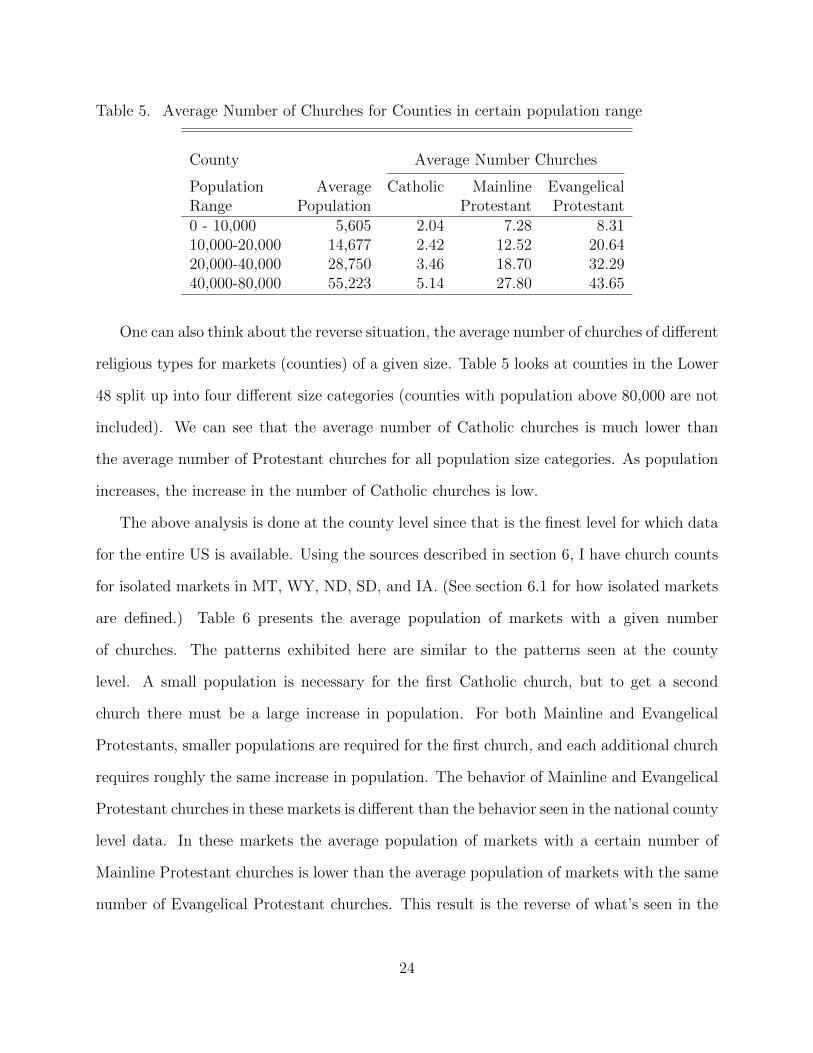
Table 5. Average Number of Churches for Counties in certain population range

County Average Number Churches

Population Average Catholic Mainline EvangelicalRange Population Protestant Protestant0 - 10,000 5,605 2.04 7.28 8.3110,000-20,000 14,677 2.42 12.52 20.6420,000-40,000 28,750 3.46 18.70 32.2940,000-80,000 55,223 5.14 27.80 43.65

One can also think about the reverse situation, the average number of churches of different

religious types for markets (counties) of a given size. Table 5 looks at counties in the Lower

48 split up into four different size categories (counties with population above 80,000 are not

included). We can see that the average number of Catholic churches is much lower than

the average number of Protestant churches for all population size categories. As population

increases, the increase in the number of Catholic churches is low.

The above analysis is done at the county level since that is the finest level for which data

for the entire US is available. Using the sources described in section 6, I have church counts

for isolated markets in MT, WY, ND, SD, and IA. (See section 6.1 for how isolated markets

are defined.) Table 6 presents the average population of markets with a given number

of churches. The patterns exhibited here are similar to the patterns seen at the county

level. A small population is necessary for the first Catholic church, but to get a second

church there must be a large increase in population. For both Mainline and Evangelical

Protestants, smaller populations are required for the first church, and each additional church

requires roughly the same increase in population. The behavior of Mainline and Evangelical

Protestant churches in these markets is different than the behavior seen in the national county

level data. In these markets the average population of markets with a certain number of

Mainline Protestant churches is lower than the average population of markets with the same

number of Evangelical Protestant churches. This result is the reverse of what’s seen in the

24

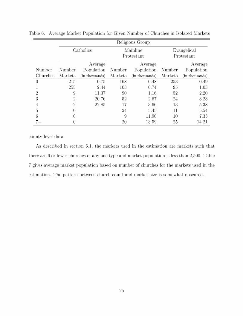
Table 6. Average Market Population for Given Number of Churches in Isolated Markets

Religious Group

Catholics Mainline EvangelicalProtestant Protestant

Average Average AverageNumber Number Population Number Population Number PopulationChurches Markets (in thousands) Markets (in thousands) Markets (in thousands)

0 215 0.75 168 0.48 253 0.491 255 2.44 103 0.74 95 1.032 9 11.37 90 1.16 52 2.203 2 20.76 52 2.67 24 3.234 2 22.85 17 3.66 13 5.385 0 24 5.45 11 5.546 0 9 11.90 10 7.337+ 0 20 13.59 25 14.21

county level data.

As described in section 6.1, the markets used in the estimation are markets such that

there are 6 or fewer churches of any one type and market population is less than 2,500. Table

7 gives average market population based on number of churches for the markets used in the

estimation. The pattern between church count and market size is somewhat obscured.

25

Table 7. Average Market Population for Given Number of Churches (markets with popu-lation below 2,500)

Religious Group

Catholics Mainline EvangelicalProtestant Protestant

Average Average AverageNumber Number Population Number Population Number PopulationChurches Markets (in thousands) Markets (in thousands) Markets (in thousands)

0 206 0.41 164 0.41 252 0.291 190 1.06 100 0.67 92 0.932 3 1.58 84 1.01 36 1.433 0 36 1.34 10 1.674 0 10 1.46 4 1.915 0 5 1.50 3 1.716 0 0 2 2.24

8 Results

I first present the estimates to the game presented above. I then use the parameter estimates

in experiments where I consider Catholic churches to be just like Protestant churches except

for the existence of a planner.

8.1 Estimates

I estimate the game presented in section 4 using the strategy described in section 5 . Specif-

ically, I estimate the inter-religious game between Mainline and Evangelical Protestants, so

R = MP,EP. I also make the assumption that both of these religious groups are acting

under decentralized entry. Thus I set λr = 0 for both MP and EP in equation 5. I estimate

the restricted model in which the αnr ’s are set so that variable profits are evenly split between

Nr churches. I also estimate the case where the αnr ’s are free, so that variable profits decrease

as Nr increases, but not necessarily in exact proportion. (I do impose the restriction that

(1−∑Nmax

rn=2 αn

r ≥ 0) so that per church profits are always positive.)

26

The specific markets used were markets in MT, WY, ND, SD, and IA. The restrictions

on market population result in markets such that the maximum number of churches of a

specific religious type in a certain market is 6. This maximum on number of churches is

necessary for estimation, since each αnr needs to be estimated (there must be a limit on the

maximum number of churches). Table 2 gives summary statistics of market characteristics

for these markets used in the estimation. The characteristics for this set of markets are

similar to those for the set of isolated markets in MT, WY, ND, SD, and IA.

Table 8 gives the results of the estimation. The estimates for the two cases (with α’s

restricted and not restricted) are qualitatively similar. The estimates for βr, δr, α2r , . . . , α

5r , γ

r

for r = MP,EP are all significant at the 5% level. The αnr terms are lower for EP than

MP . This implies additional EP churches have lower adverse effects on existing entrants.

The fixed cost for an EP church is larger than the fixed cost of an MP church. The cross-

effect terms, θMP,EP and θEP,MP are also both significant at the 5% level. They are negative,

as would be expected for the competitive effects of another firm.

8.2 Experiments

It was seen in section 7 that Catholic churches are behaving quite differently than Protestant

churches. This section looks at the effect of a planner making entry decisions compared to

decentralized entry. The estimates in section 8 were obtained making the assumption that

Protestant churches were taking part in decentralized entry (this means that a Protestant

church’s marginal profit given in equation (5) has λMP = λEP = 0). In this section I want to

see to what extent a Catholic planner explains the difference in entry behavior. Specifically,

I will address the question: if Catholics are exactly like Mainline Protestants (parameters are

those estimated for MP above) except Catholics are being run by a planner (Catholics have

marginal profit given by equation 5 with λC = 1) what would the Catholic entry pattern look

like? This experiment will be repeated treating Catholics just like Evangelical Protestants,

27

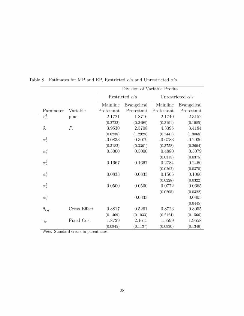
Table 8. Estimates for MP and EP, Restricted α’s and Unrestricted α’s

Division of Variable Profits

Restricted α’s Unrestricted α’s

Mainline Evangelical Mainline EvangelicalParameter Variable Protestant Protestant Protestant Protestantβ1r pinc 2.1721 1.8716 2.1740 2.3152

(0.2722) (0.2498) (0.3191) (0.1985)

δr Fr 3.9530 2.5708 4.3395 3.4184(0.6238) (1.2928) (0.7441) (1.3068)

α1r -0.0833 0.3079 -0.6783 -0.2936

(0.3182) (0.3361) (0.3758) (0.2604)

α2r 0.5000 0.5000 0.4880 0.5079

(0.0315) (0.0375)

α3r 0.1667 0.1667 0.2784 0.2460

(0.0262) (0.0370)

α4r 0.0833 0.0833 0.1565 0.1066

(0.0228) (0.0322)

α5r 0.0500 0.0500 0.0772 0.0665

(0.0205) (0.0322)

α6r 0.0333 0.0805

(0.0445)

θr,q Cross Effect 0.8817 0.5261 0.8723 0.8055(0.1469) (0.1033) (0.2124) (0.1566)

γr Fixed Cost 1.8729 2.1615 1.5599 1.9658(0.0945) (0.1137) (0.0930) (0.1346)

Note: Standard errors in parentheses.

28

Table 9. Probability a Market has given number of churches, using MP estimates, givendifferent λC

Number Restricted α’s Unrestricted α’s

Churches Actual λC = 0 λC = 1 λC = 0 λC = 10 0.52 0.44 0.44 0.52 0.521 0.48 0.20 0.53 0.20 0.462 0.01 0.12 0.00 0.18 0.013 0.00 0.07 0.00 0.07 0.004 0.00 0.04 0.00 0.01 0.005 0.00 0.13 0.03 0.02 0.00

except for the λC term.

Using the parameter estimates from section 8 and assuming a value for λC I will obtain

fitted values for the number of Catholic churches in each market. The per-capita variable

profit for a Catholic church is given by:

VC(X,FC) = δrFC +Xβr + α1r (10)

The profit of the N thC Catholic church will be given by:

ΠC(NC , Z, ωr;λC) =

(1−

N∑n=2

αnr

)VC(X,FC)S − γr − λC(NC − 1)αN VC(X,FC)S (11)

This marginal profit equation is very similar to equation 5. The cross-effect of MP or EP

churches has been set to 0 (θC,MP = θC,EP = 0). Using the profit function given in equation

(11), I can obtain a probability mapping similar to Ψ in equation (9). I use this probability

mapping to produce the probability of there being NC Catholic churches, assuming Catholics

have the same parameters as MP , for the cases λC = 0 and also if λC = 1. Table 9 reports

the results, along with the probabilities actually seen in the data. Notice that changing λC

from 0 to 1 does not change the probability of there being 0 Catholic churches. Looking at

profit equation 11, it can be seen that ΠC(1, Z, ωr;λC) is not affected at all by the λC term.

29

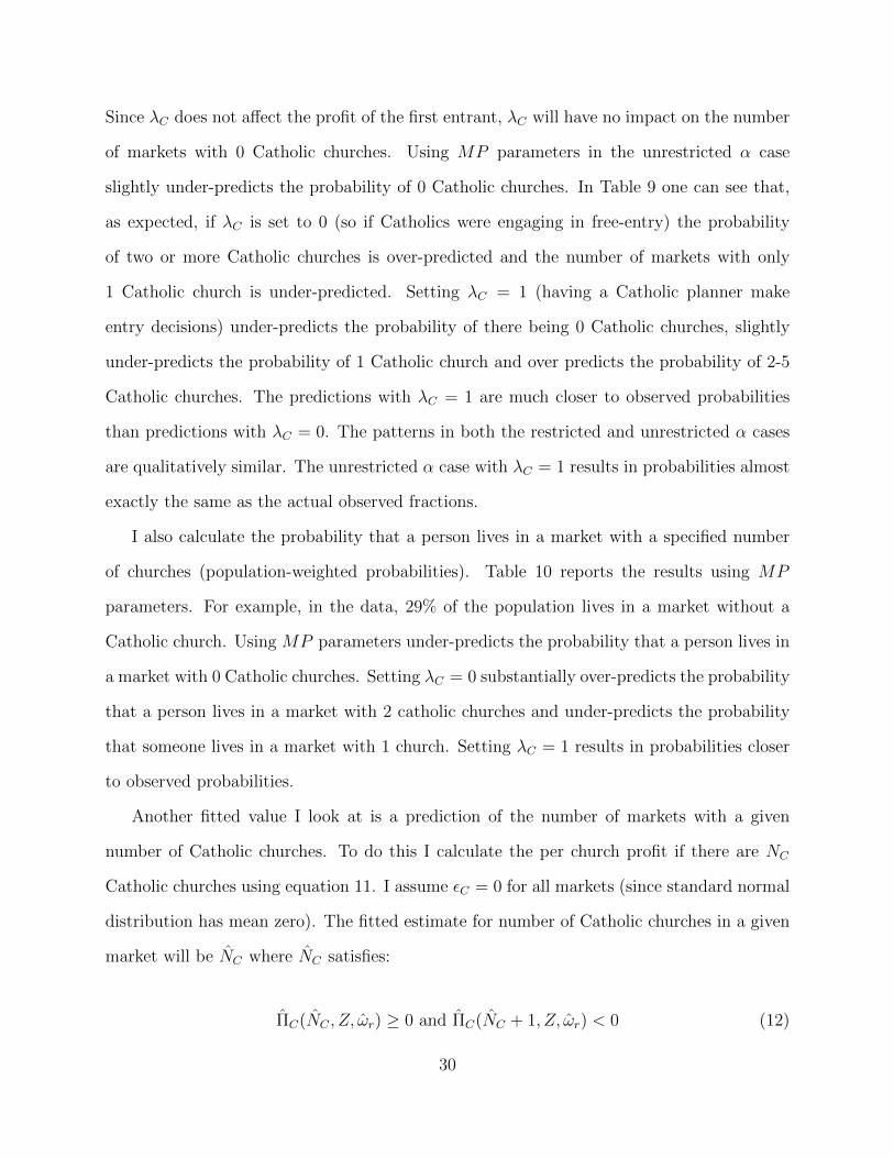
Since λC does not affect the profit of the first entrant, λC will have no impact on the number

of markets with 0 Catholic churches. Using MP parameters in the unrestricted α case

slightly under-predicts the probability of 0 Catholic churches. In Table 9 one can see that,

as expected, if λC is set to 0 (so if Catholics were engaging in free-entry) the probability

of two or more Catholic churches is over-predicted and the number of markets with only

1 Catholic church is under-predicted. Setting λC = 1 (having a Catholic planner make

entry decisions) under-predicts the probability of there being 0 Catholic churches, slightly

under-predicts the probability of 1 Catholic church and over predicts the probability of 2-5

Catholic churches. The predictions with λC = 1 are much closer to observed probabilities

than predictions with λC = 0. The patterns in both the restricted and unrestricted α cases

are qualitatively similar. The unrestricted α case with λC = 1 results in probabilities almost

exactly the same as the actual observed fractions.

I also calculate the probability that a person lives in a market with a specified number

of churches (population-weighted probabilities). Table 10 reports the results using MP

parameters. For example, in the data, 29% of the population lives in a market without a

Catholic church. Using MP parameters under-predicts the probability that a person lives in

a market with 0 Catholic churches. Setting λC = 0 substantially over-predicts the probability

that a person lives in a market with 2 catholic churches and under-predicts the probability

that someone lives in a market with 1 church. Setting λC = 1 results in probabilities closer

to observed probabilities.

Another fitted value I look at is a prediction of the number of markets with a given

number of Catholic churches. To do this I calculate the per church profit if there are NC

Catholic churches using equation 11. I assume εC = 0 for all markets (since standard normal

distribution has mean zero). The fitted estimate for number of Catholic churches in a given

market will be NC where NC satisfies:

ΠC(NC , Z, ωr) ≥ 0 and ΠC(NC + 1, Z, ωr) < 0 (12)

30

Table 10. Probability a Person lives in a Market with a given number of churches, usingMP estimates, for different λC

Number Restricted α’s Unrestricted α’s

Churches Actual λC = 0 λC = 1 λC = 0 λC = 10 0.29 0.16 0.16 0.23 0.231 0.69 0.20 0.81 0.25 0.762 0.02 0.18 0.00 0.34 0.013 0.00 0.13 0.00 0.14 0.004 0.00 0.08 0.00 0.02 0.005 0.00 0.24 0.03 0.02 0.00

Table 11. Estimated Number Markets with Given Number of Catholic Churches, usingMP parameter estimates, for given λC

Number of Markets

Number Restricted α’s Unrestricted α’s

Churches Actual λC = 0 λC = 1 λC = 0 λC = 10 206 196 196 227 2271 190 69 203 82 1722 3 65 0 83 03 0 37 0 7 04 0 18 0 0 05 0 14 0 0 0

Table 11 reports the fitted values using MP parameters. The number of markets with

0 Catholic churches is under-predicted in the restricted α case and over-predicted in the

unrestricted α case. As expected, when λC = 0, the number of markets with 1 Catholic

church is substantially under-predicted and the number of markets with 2 or more Catholic

churches is over predicted. Predictions with λC = 1 are much closer to the data.

The above experiments are also done using EP parameters and λC = 0 and λC = 1.

Tables 12, 13, and 14 report the results. We can see the pattern that the predicted probability

of 1 Catholic church is lower in the λC = 0 case than the λC = 1, while the probability of 2

or more Catholic churches is higher in the λC = 0 than the λC = 1 case. The probabilities

with unrestricted α’s and λC = 1 are nearly exactly the same as the fractions observed in

31

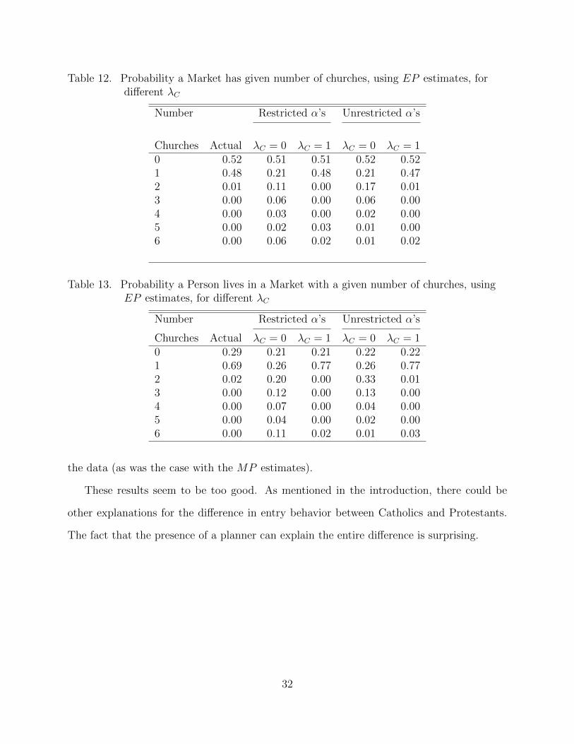
Table 12. Probability a Market has given number of churches, using EP estimates, fordifferent λC

Number Restricted α’s Unrestricted α’s

Churches Actual λC = 0 λC = 1 λC = 0 λC = 10 0.52 0.51 0.51 0.52 0.521 0.48 0.21 0.48 0.21 0.472 0.01 0.11 0.00 0.17 0.013 0.00 0.06 0.00 0.06 0.004 0.00 0.03 0.00 0.02 0.005 0.00 0.02 0.03 0.01 0.006 0.00 0.06 0.02 0.01 0.02

Table 13. Probability a Person lives in a Market with a given number of churches, usingEP estimates, for different λC

Number Restricted α’s Unrestricted α’s

Churches Actual λC = 0 λC = 1 λC = 0 λC = 10 0.29 0.21 0.21 0.22 0.221 0.69 0.26 0.77 0.26 0.772 0.02 0.20 0.00 0.33 0.013 0.00 0.12 0.00 0.13 0.004 0.00 0.07 0.00 0.04 0.005 0.00 0.04 0.00 0.02 0.006 0.00 0.11 0.02 0.01 0.03

the data (as was the case with the MP estimates).

These results seem to be too good. As mentioned in the introduction, there could be

other explanations for the difference in entry behavior between Catholics and Protestants.

The fact that the presence of a planner can explain the entire difference is surprising.

32

Table 14. Estimated Number of Catholic Churches in a Market, using EP parameter esti-mates

Number of Markets

Number Unrestricted α’s Restricted α’s

Churches Actual λC = 0 λC = 1 λC = 0 λC = 10 206 223 223 222 2221 190 82 176 83 1772 3 51 0 82 03 0 31 0 12 04 0 8 0 0 05 0 4 0 0 06 0 0 0 0 0

9 Conclusion

This paper takes the existing knowledge capital that IO economists have acquired studying

strategic entry and applies it to churches. Observing differences in the behavior of Catholic

churches compared to Mainline and Evangelical Protestant churches, this paper addresses

the question of how much of that difference can be explained by the presence of a Catholic

planner. To address this question, this paper develops a strategic entry model for churches

and estimates the model using data on uniquely defined markets. Assuming that Catholics

are just like Protestants, other than being centrally planned, I find that a Catholic planner

explains virtually all of the difference in entry patterns.

It could be argued that this the presence of a planner explains too much of the difference

in behavior. There are other differences in between Catholics and Protestants that could

potentially explain the difference in entry behavior. One possibility is a Protestant preference

for fewer members per church. Potential future research includes introducing a demand

structure into the model to address other possible explanations.

33

References

US religious landscape survey religious beliefs and practices: diverse and politically relevant.

Pew Forum on Religion and Public Life, 2008.

V. Aguirregabiria and P. Mira. Sequential Estimation of Dynamic Discrete Games. Econo-

metrica, 75(1):1–54, 2007.

N. Ammerman. Doing Good in American Communities: Congregations and Service Orga-

nizations Working Together. 2001.

S. Anderson and A. De Palma. The Logit as a Model of Product Differentiation. Oxford

Economic Papers, 44(1):51–67, 1992.

C. Azzi and R. Ehrenberg. Household Allocation of Time and Church Attendance. The

Journal of Political Economy, 83(1):27–56, 1975.

S. Berry and P. Reiss. Empirical Models of Entry and Market Structure. Handbook of

Industrial Organization, 3, 2007.

S. Berry and J. Waldfogel. Free Entry and Social Inefficiency in Radio Broadcasting. Rand

Journal of Economics, 30:397–420, 1999.

T. Bresnahan and P. Reiss. Entry and Competition in Concentrated Markets. The Journal

of Political Economy, 99(5):977–1009, 1991.

R. Ekelund. Sacred Trust: The Medieval Church as an Economic Firm. Oxford University

Press, USA, 1996.

R. Finke and C. Scheitle. Accounting for the Uncounted: Computing Correctives for the

2000 RCMS Data. Review of Religious Research, 47(1):5, 2005.

34

J. Gruber. Religious Market Structure, Religious Participation, and Outcomes: Is Religion

Good for You? NBER Working Paper, 11377, 2005.

T. Holmes and S. Lee. Cities as Six-by-Six Mile Squares: Zipfs Law? University of Minnesota

Working Paper, 2007.

C. Hsieh and E. Moretti. Can Free Entry Be Inefficient? Fixed Commissions and Social

Waste in the Real Estate Industry. Journal of Political Economy, 111(5):1076–1122, 2003.

L. Iannaccone. Introduction to the Economics of Religion. Journal of Economic Literature,

36(3):1465–1495, 1998.

D. E. Jones, S. Doty, C. Grammich, J. E. Horsch, R. Houseal, M. Lynn, J. P. Marcum, K. M.

Sanchagrin, and R. H. Taylor. Religious Congregations and Membership in the United

States, 2000: An Enumeration by Region, State and County Based on Data Reported for

149 Religious Bodies. Nashville: Glenmary Research Center, 2002.

J. Lipford. Organizational reputation and constitutional constraints: An application to

religious denominations. Constitutional Political Economy, 3(3):343–357, 1992.

M. Loveland. Religious Switching: Preference Development, Maintenance, and Change.

Journal for the Scientific Study of Religion, 42(1):147–157, 2003.

N. Mankiw and M. Whinston. Free Entry and Social Inefficiency. Rand Journal of Eco-

nomics, 17(1):48–58, 1986.

R. Mitchell. Polity, Church Attractiveness, and Ministers’ Careers: An Eight-Denomination

Study of Interchurch Mobility. 2007.

J. Montgomery. Dynamics of the Religious Economy: Exit, Voice and Denominational

Secularization. Rationality and Society, 8(1):81, 1996.

35

K. Seim. Spatial Differentiation and Market Structure: The Video Retail Industry. PhD

thesis, Yale University, 2001.

A. Smith. The wealth of nations (1991 edition), 1776.

R. Stonebraker. Optimal Church Size: The Bigger the Better? Journal for the Scientific

Study of Religion, 32:231–231, 1993.

K. Takayama. Formal polity and change of structure: Denominational assemblies. Sociolog-

ical Analysis, 36(1):17–28, 1975.

A Proof

Proposition A.1. With consumer utility given in equation (1), fixed price p for every

church, the number of churches in market with free-entry, NF , will be greater than or equal

to the number of churches chosen by a planner, NP .

Proof. Given a market with population S, if there are N churches each church will attract

an equal number of customers:

S

N + exp[(V0 − a+ p)/µ]

Given constant price p, profit for each church will be:

ΠN =pS

N + c− γ

Where c = exp[(V0− a+ p)/µ]. We can see that ΠN is decreasing in number of churches, N .

In free-entry the number of churches, NF , will satisfy a zero-profit condition:

ΠNF ≥ 0 and ΠNF +1 < 0

36

With a planner, the number of churches, NP , must maximize total profit:

(NP + 1)ΠNP +1 < NPΠNP ≥ (NP − 1)ΠNP−1

This condition can be re-written as:

ΠNP −(NP − 1)pS

(NP + c)(NP + c− 1)≥ 0 and ΠNP +1 −

NP pS(NP + 1 + c

)(NP + c

) < 0

Comparing this condition to the free-entry condition highlights that the planner takes into

account the profits of the last church and also the negative effect of that last church on

existing churches (the (NP−1)pS

(NP +c)(NP +c−1)term). In free-entry each entrant only considers its

own profits, not its effect on others.

Since NpS(N+c+1)(N+c)

≥ 0 for N ≥ 1, it follows that ΠN+1− NpS(N+c+1)(N+c)

≤ ΠN+1 for N ≥ 1.

Thus the number of churches that satisfies the planner’s condition, NP , is less than or equal

to the number of churches that satisfies the free-entry condition, NF .

B Data Appendix

B.1 Market Definition

I start with the 3,877,307 Census blocks that are in the lower 48 states and the District

of Columbia and not in a Metropolitan Statistical Area (MSA). I begin with each of these

3,877,307 blocks as a potential ’center’ for a market. For every one of these potential center

blocks I find the aggregate population of all blocks within 0.75 miles the potential center

block. I now have the three-quarter mile population of every potential center block. Take a

specific potential center block, called block A. For block A I find all other potential center

blocks within 12 miles of A. Let UA denote this set of all potential center blocks within

37

12 miles of block A. I am interested in the block in the set UA that has the maximum

population; call this block mA. Every potential center has a corresponding mA (so there are

3,877,307). Out of this set of 3,877,307 mA’s there will be many duplicates. After duplicates

are eliminated, I go through each mA and compare it to all other mA’s. If any two mA’s

are within 12 miles of each other the mA with a smaller population is eliminated. After this

process I am left with a set of blocks that I consider to be ‘centers.’ There are 5,586 centers.

Every state but New Jersey has at least one center. I consider a market to be everything

within 3 miles of these centers.

38