RELIABLE USER DATAGRAM PROTOCOL (RUDP) by ABHILASH ...

RELIABLE USER DATAGRAM PROTOCOL (RUDP)

by

ABHILASH THAMMADI

B.ENGG., OSMANIA UNIVERSITY, INDIA, 2009

A REPORT

submitted in partial fulfillment of the requirements for the degree

MASTER OF SCIENCE

Department of Computing and Information Sciences

College of Engineering

KANSAS STATE UNIVERSITY

Manhattan, Kansas

2011

Approved by:

Major Professor

Dr. Gurdip Singh

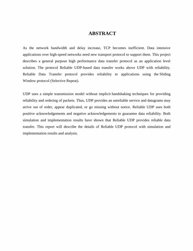
ABSTRACT

As the network bandwidth and delay increase, TCP becomes inefficient. Data intensive

applications over high-speed networks need new transport protocol to support them. This project

describes a general purpose high performance data transfer protocol as an application level

solution. The protocol Reliable UDP-based data transfer works above UDP with reliability.

Reliable Data Transfer protocol provides reliability to applications using the Sliding

Window protocol (Selective Repeat).

UDP uses a simple transmission model without implicit handshaking techniques for providing

reliability and ordering of packets. Thus, UDP provides an unreliable service and datagrams may

arrive out of order, appear duplicated, or go missing without notice. Reliable UDP uses both

positive acknowledgements and negative acknowledgements to guarantee data reliability. Both

simulation and implementation results have shown that Reliable UDP provides reliable data

transfer. This report will describe the details of Reliable UDP protocol with simulation and

implementation results and analysis.

iii

TABLE OF CONTENTS

TABLE OF CONTENTS ....................................................................................... iii

LIST OF FIGURES ............................................................................................... iv

ACKNOWLEDGEMENTS .................................................................................... v

CHAPTER 1: INTRODUCTION ........................................................................... 1

CHAPTER 2: SLIDING WINDOW PROTOCOLS .............................................. 3

2.1 One-Bit Sliding Window Protocol ................................................................ 3

2.2 Go-Back N Protocol ...................................................................................... 4

2.3 Selectve repeat Protocol ................................................................................ 5

CHAPTER 3: IMPLEMENTATION ..................................................................... 8

3.1 RUDP Protocol Archtecture ......................................................................... 8

3.2 Pseudo Code ............................................................................................... 15

CHAPTER 4: EVALUATION ............................................................................. 18

CHAPTER 5: CONCLUSION AND FUTURE WORK ...................................... 37

CHAPTER 6: REFERENCES .............................................................................. 38

iv

LIST OF FIGURES

Figure 1: Go Back N Protocol for the case in which receiver’s window is large ........................... 5

Figure 2: Example of Selective Repeat Protocol ............................................................................ 6

Figure 3: RUDP Protocol Architecture ........................................................................................... 8

Figure 4: Class Diagram ............................................................................................................... 10

Figure 5: Sender side code architecture ........................................................................................ 12

Figure 6: Receiver side code architecture ..................................................................................... 13

Figure 7: Example of the working of the RUDP protocol ............................................................ 14

Figure 8: Data Transfer Time Vs Loss Rate (Local Machine) ..................................................... 19

Figure 9: Data Transfer Time Vs Packet size (Local Machine) ................................................... 20

Figure 10: Data Transfer Time Vs Packet size (iPAQs located side by side) .............................. 20

Figure 11: Data Transfer Time Vs Packet size (iPAQs located in different rooms) .................... 21

Figure 12: Data Transfer Time Vs Network Delay (Local Machine) ........................................... 22

Figure 13: Data Transfer Time Vs Network Delay (iPAQs located side by side) ........................ 23

Figure 14: Data Transfer Time Vs Network Delay (iPAQs located in different rooms) .............. 23

Figure 15: Data Transfer Time Vs Total Data sent (Local Machine) ........................................... 25

Figure 16: Data Transfer Time Vs Total Data sent (iPAQs located side by side) ........................ 25

Figure 17: Data Transfer Time Vs Total Data sent (iPAQs located in different rooms) .............. 26

Figure 18: Time gap between packets sent Vs Rate (# received packets / # sent packets) .......... 28








Figure 26: Data Transfer Time Vs Buffer Utlization (Local Machine) ........................................ 34

Figure 27: Data Transfer Time Vs Buffer Utlization (iPAQ devices) .......................................... 34

Figure 28: Data Transfer Time Vs Total Data sent (iPAQ devices) ............................................. 36

Figure 29: Data Transfer Time Vs Packet Size (iPAQ devices) ................................................... 36

v

ACKNOWLEDGEMENTS

My special thanks to my major professor Dr. Gurdip Singh for giving me timely advice,

encouragement, and guidance throughout the project.

I would also like to thank Dr. Daniel Andresen and Dr. Torben Amtoft for graciously accepting

to serve on my committee.

Finally, I would like to thank the administrative and technical support staff of the department of

CIS and my family and friends for their support throughout my graduate study.

1

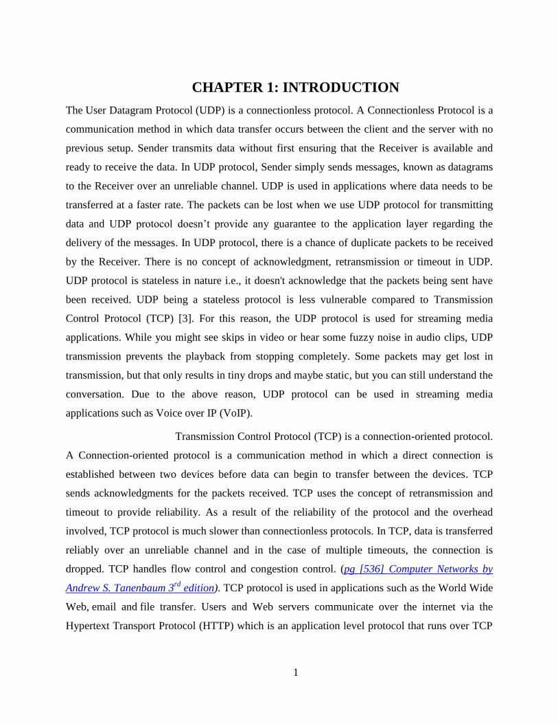
CHAPTER 1: INTRODUCTION

The User Datagram Protocol (UDP) is a connectionless protocol. A Connectionless Protocol is a

communication method in which data transfer occurs between the client and the server with no

previous setup. Sender transmits data without first ensuring that the Receiver is available and

ready to receive the data. In UDP protocol, Sender simply sends messages, known as datagrams

to the Receiver over an unreliable channel. UDP is used in applications where data needs to be

transferred at a faster rate. The packets can be lost when we use UDP protocol for transmitting

data and UDP protocol doesn’t provide any guarantee to the application layer regarding the

delivery of the messages. In UDP protocol, there is a chance of duplicate packets to be received

by the Receiver. There is no concept of acknowledgment, retransmission or timeout in UDP.

UDP protocol is stateless in nature i.e., it doesn't acknowledge that the packets being sent have

been received. UDP being a stateless protocol is less vulnerable compared to Transmission

Control Protocol (TCP) [3]. For this reason, the UDP protocol is used for streaming media

applications. While you might see skips in video or hear some fuzzy noise in audio clips, UDP

transmission prevents the playback from stopping completely. Some packets may get lost in

transmission, but that only results in tiny drops and maybe static, but you can still understand the

conversation. Due to the above reason, UDP protocol can be used in streaming media

applications such as Voice over IP (VoIP).

Transmission Control Protocol (TCP) is a connection-oriented protocol.

A Connection-oriented protocol is a communication method in which a direct connection is

established between two devices before data can begin to transfer between the devices. TCP

sends acknowledgments for the packets received. TCP uses the concept of retransmission and

timeout to provide reliability. As a result of the reliability of the protocol and the overhead

involved, TCP protocol is much slower than connectionless protocols. In TCP, data is transferred

reliably over an unreliable channel and in the case of multiple timeouts, the connection is

dropped. TCP handles flow control and congestion control. (pg [536] Computer Networks by

Andrew S. Tanenbaum 3rd

edition). TCP protocol is used in applications such as the World Wide

Web, email and file transfer. Users and Web servers communicate over the internet via the

Hypertext Transport Protocol (HTTP) which is an application level protocol that runs over TCP

2

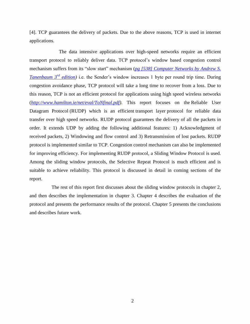
[4]. TCP guarantees the delivery of packets. Due to the above reasons, TCP is used in internet

applications.

The data intensive applications over high-speed networks require an efficient

transport protocol to reliably deliver data. TCP protocol’s window based congestion control

mechanism suffers from its “slow start” mechanism (pg [538] Computer Networks by Andrew S.

Tanenbaum 3rd

edition) i.e. the Sender’s window increases 1 byte per round trip time. During

congestion avoidance phase, TCP protocol will take a long time to recover from a loss. Due to

this reason, TCP is not an efficient protocol for applications using high speed wireless networks

(http://www.hamilton.ie/net/eval/ToNfinal.pdf). This report focuses on the Reliable User

Datagram Protocol (RUDP) which is an efficient transport layer protocol for reliable data

transfer over high speed networks. RUDP protocol guarantees the delivery of all the packets in

order. It extends UDP by adding the following additional features: 1) Acknowledgment of

received packets, 2) Windowing and flow control and 3) Retransmission of lost packets. RUDP

protocol is implemented similar to TCP. Congestion control mechanism can also be implemented

for improving efficiency. For implementing RUDP protocol, a Sliding Window Protocol is used.

Among the sliding window protocols, the Selective Repeat Protocol is much efficient and is

suitable to achieve reliability. This protocol is discussed in detail in coming sections of the

report.

The rest of this report first discusses about the sliding window protocols in chapter 2,

and then describes the implementation in chapter 3. Chapter 4 describes the evaluation of the

protocol and presents the performance results of the protocol. Chapter 5 presents the conclusions

and describes future work.

http://www.hamilton.ie/net/eval/ToNfinal.pdf

http://en.wikipedia.org/wiki/Transport_layer

http://en.wikipedia.org/wiki/Communications_protocol

3

CHAPTER 2: SLIDING WINDOW PROTOCOLS

Sliding Window Protocol is a packet-based data transmission protocol which delivers data

through messages reliably. Sliding window protocols are used where reliability and in-order

delivery of packets is required. In Sliding window protocol data is divided into segments and

packets are prepared from each segment. Sender assigns each packet, a unique sequence number

and sends it over the network. When the Receiver receives the packet, it uses the sequence

number and checks its checksum and delivers the packets to the application layer in the correct

order. Depending on the checksum, Receiver discards duplicate packets and sends

acknowledgements for the correctly received packets. A sliding window protocol allows an

unlimited number of packets to be transmitted using fixed size sequence numbers.

Sliding window protocols use the technique known as piggybacking. In this

technique, acknowledgements are attached to the next frame that is being sent out. The main

advantage of using piggybacking is to use the available channel bandwidth effectively. In the

sliding window protocol, both the Sender and the Receiver maintains a set of sequence numbers

corresponding to frames within a window of same size or different sizes. Whenever a new packet

is Sent by the Sender, it is given the next highest sequence number, and the upper edge of the

window is incremented by one. When an acknowledgement is received by the Sender, the lower

edge of the window is advanced by one. In this way the window continuously maintains a list of

unacknowledged frames. Since the data can be delivered reliably, sliding window protocols are

used for data intensive applications over high speed networks.

There are three sliding window protocols: 1) One-Bit sliding window protocol 2)

Go Back N protocol and 3) Selective Repeat protocol. The three protocols differ among

themselves in terms of efficiency, complexity, and buffer requirements. The description of the

three sliding window protocols is given below.

2.1 A One-Bit Sliding Window Protocol

One-Bit Sliding Window Protocol uses stop-and-wait protocol. This protocol has a maximum

window size of 1. In this protocol, the Sender sends a frame and waits for its acknowledgement

before sending the next frame. In this protocol, either the sender or the receiver sends the first

frame. When this frame is received, the receiver checks whether the received frame is a duplicate

4

or not. If the frame is the one expected, it is sent to the application layer. The acknowledgement

field of the header contains the sequence number of the last correctly received frame. The Sender

sends the next packet only after checking the acknowledgement number of the last correctly

received frame with the sequence number of the packet, it is trying to send. If the sequence

number disagrees, Sender retransmits the same frame again. In this protocol, whenever a frame is

received, a frame is also sent back.

An unusual situation may arise if both sender and receiver simultaneously send

the first packet. In this situation, half of the frames contain duplicates, even though there are no

transmission errors. In the case of multiple premature timeouts, duplicate frames may be sent.

2.2 Go-Back N Protocol

In One-Bit sliding window protocol, the round trip time i.e., the time taken for a sent packet to be

received by the Receiver and acknowledged packet to be received by the Sender is assumed to be

negligible (pg [207] Computer Networks by Andrew S. Tanenbaum, Third Edition). In these

situations the long round trip time can have major effects on the efficiency of the channel

bandwidth utilization. In Go-Back N protocol, the Sender transmits up to a specified number of

frames without blocking. In this protocol, the Sender can continuously transmit frames for a

time equal to the round-trip time without filling up the window. This ability of the Sender to fill

the window without stopping is known as pipelining. Pipelining frames over an unreliable

communication channel can cause some serious issues. Consider a situation where a frame in the

middle of a long stream is damaged or lost, a large number of frames following it will be

received by the Receiver before the sender even finds out that anything is wrong. The damaged

frame received by the receiver is discarded. The serious issue here is what should be done with

the large number of correctly received frames following it. This situation can be handled by the

Go Back N protocol.

Go Back N protocol deals with the above situation and handles errors when the

frames are pipelined. In this protocol, the Receiver simply discards all the correctly received

frames following the bad frame and sends no acknowledgements for the discarded frames. This

protocol has a Receiver window of size 1. The pipeline will begin to empty, if the Sender's

window fills up before the timer expires. Eventually, the sender will time out and retransmit all

5

unacknowledged frames in order, starting with the damaged frame. This protocol can waste a lot

of bandwidth if the packet loss rate is high.

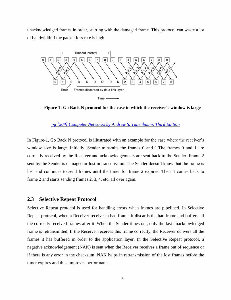
Figure 1: Go Back N protocol for the case in which the receiver's window is large

pg [208] Computer Networks by Andrew S. Tanenbaum, Third Edition

In Figure-1, Go Back N protocol is illustrated with an example for the case where the receiver’s

window size is large. Initially, Sender transmits the frames 0 and 1.The frames 0 and 1 are

correctly received by the Receiver and acknowledgements are sent back to the Sender. Frame 2

sent by the Sender is damaged or lost in transmission. The Sender doesn’t know that the frame is

lost and continues to send frames until the timer for frame 2 expires. Then it comes back to

frame 2 and starts sending frames 2, 3, 4, etc. all over again.

2.3 Selective Repeat Protocol

Selective Repeat protocol is used for handling errors when frames are pipelined. In Selective

Repeat protocol, when a Receiver receives a bad frame, it discards the bad frame and buffers all

the correctly received frames after it. When the Sender times out, only the last unacknowledged

frame is retransmitted. If the Receiver receives this frame correctly, the Receiver delivers all the

frames it has buffered in order to the application layer. In the Selective Repeat protocol, a

negative acknowledgement (NAK) is sent when the Receiver receives a frame out of sequence or

if there is any error in the checksum. NAK helps in retransmission of the lost frames before the

timer expires and thus improves performance.

6

Go- Back N Protocol is suitable in situations where loss of packets rare, but if the connectivity is

poor, then Go Back N protocol wastes a lot of bandwidth on retransmitted frames. Unlike Go

Back N protocol, Selective Repeat protocol allows the receiver to accept and buffer the frames

following a damaged frame. Unlike Go Back N protocol, Selective Repeat protocol does not

discard frames. In this protocol, both sender and receiver maintain a window of same size which

is equal to some predefined maximum to avoid the communication errors in the cases where

packets are being dropped. Whenever Receiver receives a frame, it verifies its sequence number

by the checksum function. If this frame contains data, put the frame in Receiver’s buffer and

send back an ACK to the Sender. The received frame must be kept within the Receiver’s buffer

and the frame is not sent to the application layer until all the lower-numbered frames have

already been acknowledged and delivered to the application layer in the correct order.

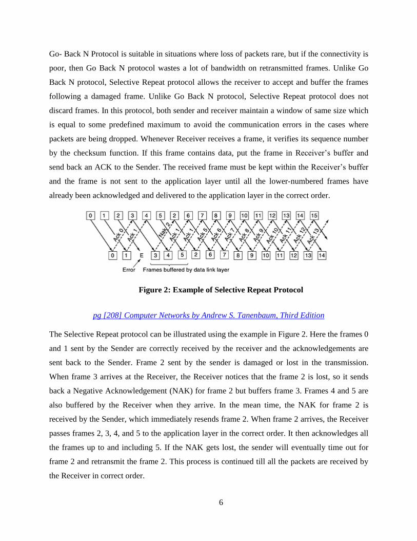
Figure 2: Example of Selective Repeat Protocol

pg [208] Computer Networks by Andrew S. Tanenbaum, Third Edition

The Selective Repeat protocol can be illustrated using the example in Figure 2. Here the frames 0

and 1 sent by the Sender are correctly received by the receiver and the acknowledgements are

sent back to the Sender. Frame 2 sent by the sender is damaged or lost in the transmission.

When frame 3 arrives at the Receiver, the Receiver notices that the frame 2 is lost, so it sends

back a Negative Acknowledgement (NAK) for frame 2 but buffers frame 3. Frames 4 and 5 are

also buffered by the Receiver when they arrive. In the mean time, the NAK for frame 2 is

received by the Sender, which immediately resends frame 2. When frame 2 arrives, the Receiver

passes frames 2, 3, 4, and 5 to the application layer in the correct order. It then acknowledges all

the frames up to and including 5. If the NAK gets lost, the sender will eventually time out for

frame 2 and retransmit the frame 2. This process is continued till all the packets are received by

the Receiver in correct order.

7

When compared to Go Back N protocol and One-Bit sliding window protocol, it has fewer

retransmissions. The limitations of Selective Repeat protocol include: 1) Selective Repeat

protocol has more complexity at the sender and the receiver. 2) In Selective Repeat protocol,

each frame must be acknowledged individually. This adds more time complexity. For the

implementation of RUDP protocol I have used Selective Repeat protocol since it is an efficient

and performance effective protocol when compared to One-Bit sliding window protocol and Go-

Back N protocol [2]. Selective Repeat protocol satisfies all the requirements for implementing

the RUDP protocol. To overcome the limitations of the sliding window protocol, Receiver uses

only positive Acknowledgement (ACK) to acknowledge the correctly received last packet.

Receiver explicitly includes the sequence number of packet being acknowledged. RUDP

protocol avoids the use of Negative Acknowledgements (NAKs) to reduce the complexity. The

architecture of the RUDP protocol and its implementation using the Selective Repeat protocol is

discussed in chapter 3.

8

CHAPTER 3: IMPLEMENTATION

3.1 RUDP Protocol Architecture

Reliable User Datagram Protocol (RUDP) is a transport layer protocol which aims to provide a

solution where UDP is too primitive because guaranteed order packet delivery is required. The

reliability is achieved using the Selective Repeat version of the Sliding Window protocol which

is described in chapter 2. Selective repeat protocol is an efficient protocol to achieve reliable

communication. Selective Repeat protocol uses acknowledgements and timeouts to achieve the

goal of reliable data transfer. RUDP protocol is designed in such a way that it also handles flow

control. The architecture of the RUDP protocol is discussed below.

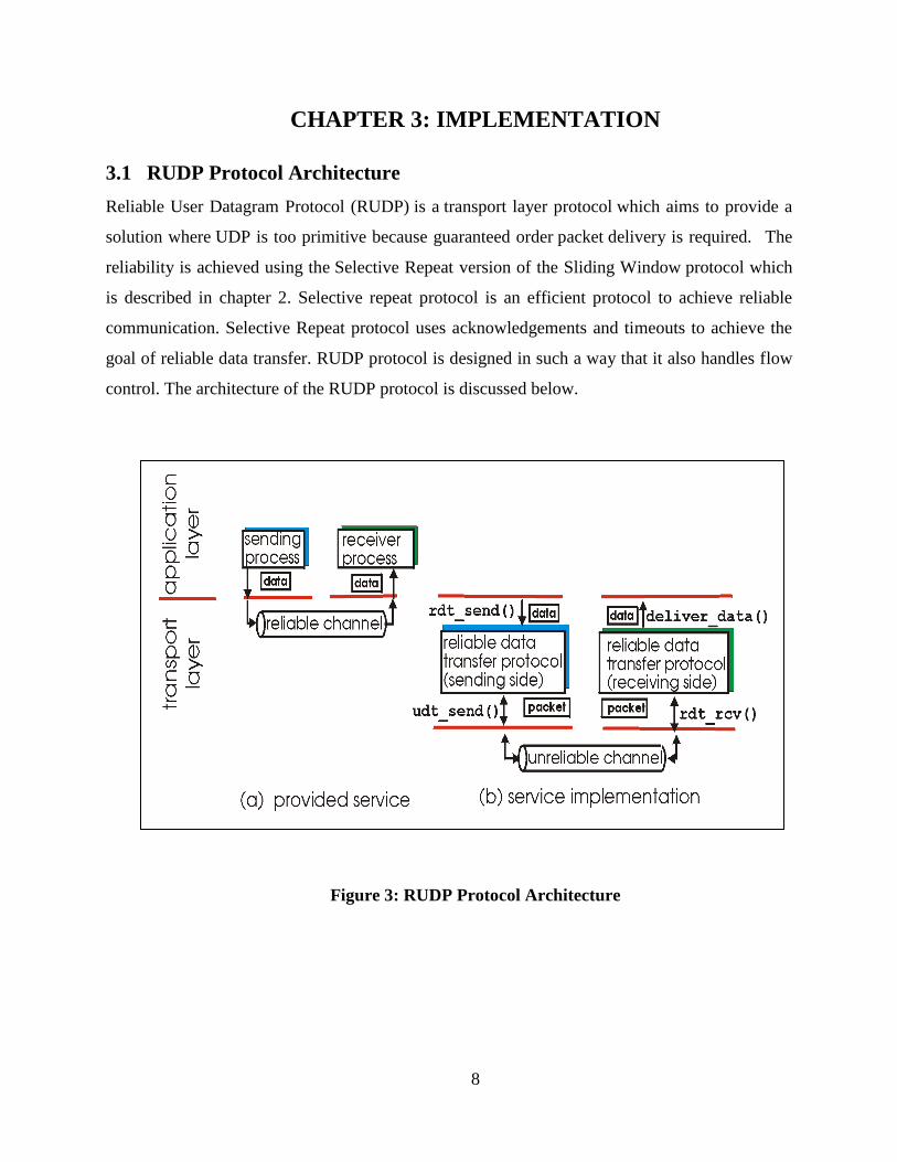
Figure 3: RUDP Protocol Architecture

9

Figure 3 presents the RUDP protocol Architecture. Figure 3 (a) gives the description of the

service provided by the protocol. The sending and receiving process are present in the

application layer. The Sender sends the data to the Receiver over the reliable channel using

RUDP protocol. Figure 3(b) gives brief description about the service implementation of the

RUDP protocol. Both the Sender and the Receiver maintain a window size of some predefined

maximum to avoid communication errors in all cases where packets are being dropped. Using

the RUDP protocol, data is sent reliably over an unreliable channel. The Sender and Receiver

side architecture is discussed in later sections of this chapter.

In the implementation of RUDP protocol, I have used synchronized shared

buffers using counting semaphores so that only one thread accesses the buffer at a time to

prevent the deadlock situation from occurring. There are two variables “base” and “next” to keep

track of the window size. If the packet is sent by the Sender, the variable next is advanced by

one. If the acknowledgement for the packet sent is received by the Sender, the variable base is

advanced by one. In this way, we can keep track of the number of packets in the buffer.

The timeouts are handled using the timers which are scheduled immediately

after sending the packet over the channel. I have simulated the packet loss rate and random

network delay in the protocol. The packets are kept in a queue before sending them over the

socket. While inserting the packets into the queue, they are assigned a value which is equal to the

system current time plus the value of the network delay. When the system current time equals to

the value associated with the packet, the packet is removed from the queue and sent it over the

network. Hence the each packet is removed from the queue after a delay and sent over the

channel. I have handled the sequence numbers in the following way. Each packet is given a

sequence number and sent over the channel by the Sender. After receiving the acknowledgement

(ACK), which has the acknowledgement number same as the sequence number of the sent

packet, Sender sends the next packet assigning it the next consecutive sequence number.

10

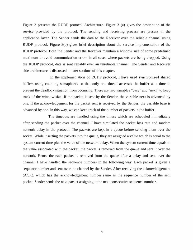
Figure 4: Class Diagram

11

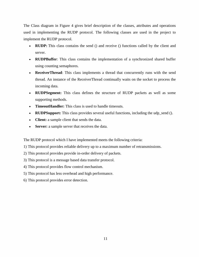
The Class diagram in Figure 4 gives brief description of the classes, attributes and operations

used in implementing the RUDP protocol. The following classes are used in the project to

implement the RUDP protocol.

RUDP: This class contains the send () and receive () functions called by the client and

server.

RUDPBuffer: This class contains the implementation of a synchronized shared buffer

using counting semaphores.

ReceiverThread: This class implements a thread that concurrently runs with the send

thread. An instance of the ReceiverThread continually waits on the socket to process the

incoming data.

RUDPSegment: This class defines the structure of RUDP packets as well as some

supporting methods.

TimeoutHandler: This class is used to handle timeouts.

RUDPSupport: This class provides several useful functions, including the udp_send ().

Client: a sample client that sends the data.

Server: a sample server that receives the data.

The RUDP protocol which I have implemented meets the following criteria:

1) This protocol provides reliable delivery up to a maximum number of retransmissions.

2) This protocol provides provide in-order delivery of packets.

3) This protocol is a message based data transfer protocol.

4) This protocol provides flow control mechanism.

5) This protocol has less overhead and high performance.

6) This protocol provides error detection.

12

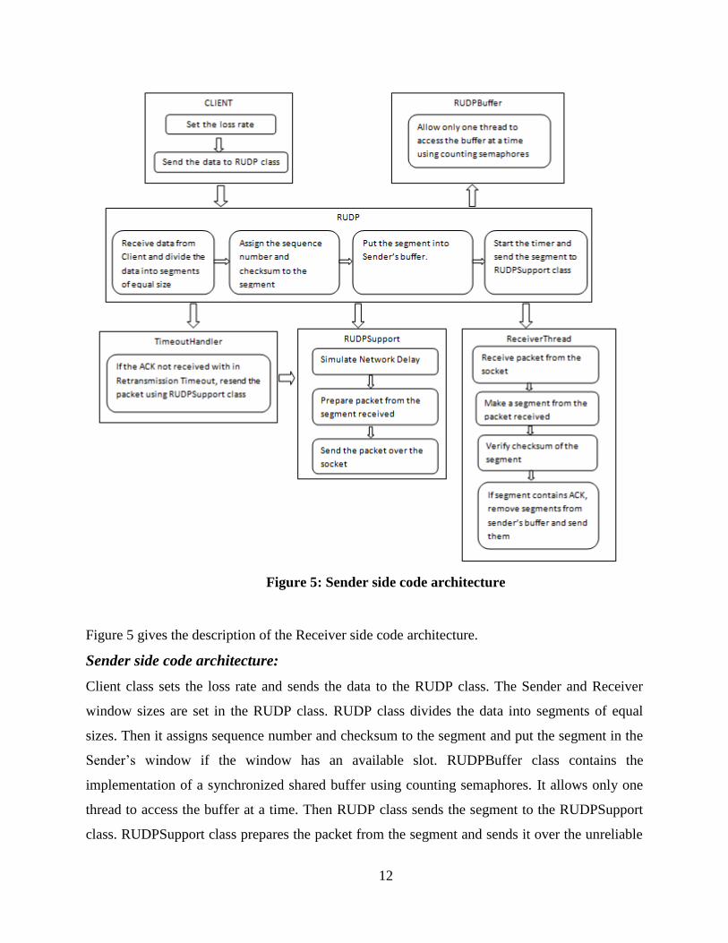
Figure 5: Sender side code architecture

Figure 5 gives the description of the Receiver side code architecture.

Sender side code architecture:

Client class sets the loss rate and sends the data to the RUDP class. The Sender and Receiver

window sizes are set in the RUDP class. RUDP class divides the data into segments of equal

sizes. Then it assigns sequence number and checksum to the segment and put the segment in the

Sender’s window if the window has an available slot. RUDPBuffer class contains the

implementation of a synchronized shared buffer using counting semaphores. It allows only one

thread to access the buffer at a time. Then RUDP class sends the segment to the RUDPSupport

class. RUDPSupport class prepares the packet from the segment and sends it over the unreliable

13

channel. The timer is started immediately after sending the packet over the unreliable channel.

ReceiverThread class implements a thread that concurrently runs with the send thread. An

instance of the ReceiverThread continually waits on the socket to process the incoming data. The

ReceiverThread class receives the packet from the socket and makes a segment from the packet

and verifies the checksum of the segment. If segment contains acknowledgement (ACK), remove

segments from the Sender’s window and send it over the socket. If a timeout happens due to the

loss of the packet, Sender resends the lost packet and restarts the timer. If the RUDP class

receives the ACK before the retransmission timeout, the timer is cancelled. The Fin flag is used

to indicate that all the data is being sent and all the ACKs have been received and the connection

is closed.

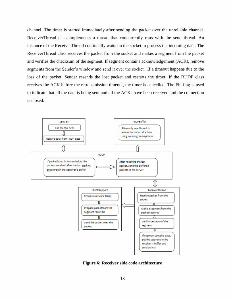
Figure 6: Receiver side code architecture

14

Sender Receiver

Figure 6 gives the description of the Receiver side code architecture.

Receiver side code architecture:

ReceiverThread class implements a thread that concurrently runs with the send thread. An

instance of the ReceiverThread continually waits on the socket to process the incoming data. The

ReceiverThread class receives the packet from the socket and makes a segment from the packet

and verifies the checksum of the segment. If the segment contains data, put the segment into the

Receiver’s buffer and send back an ACK. If a packet is lost in transmission, the RUDP class will

store all the packets following the lost packet in the Receiver’s buffer. After receiving the lost

packet, the RUDP class delivers all the packets it has buffered in correct order to Server. The Fin

flag is used here to indicate that all the data have been received and the connection is closed.

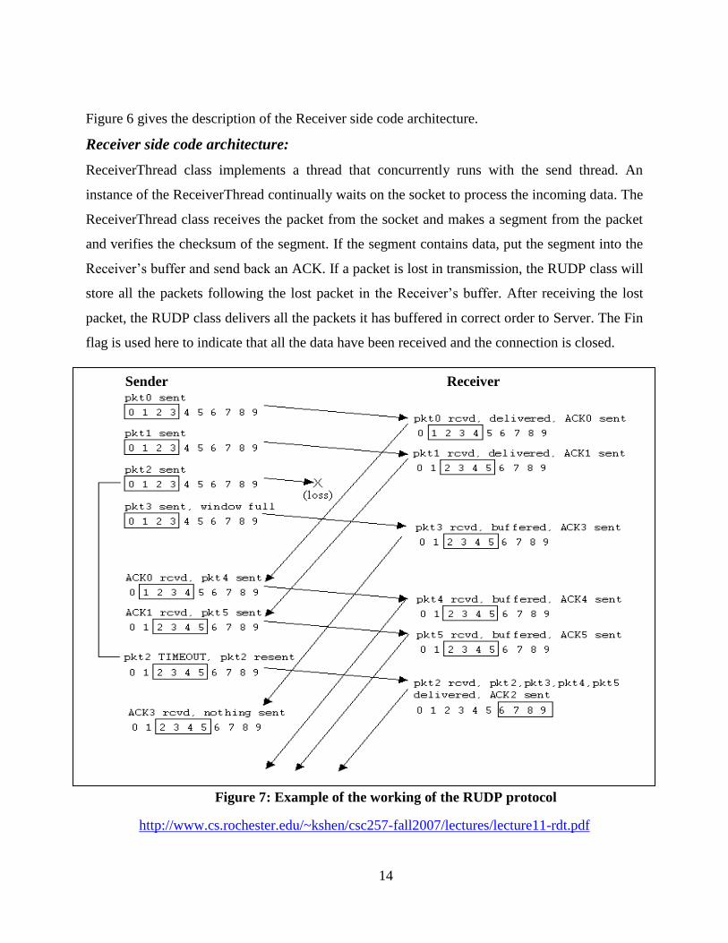
Figure 7: Example of the working of the RUDP protocol

http://www.cs.rochester.edu/~kshen/csc257-fall2007/lectures/lecture11-rdt.pdf

http://www.cs.rochester.edu/~kshen/csc257-fall2007/lectures/lecture11-rdt.pdf

15

Figure 7 gives an example of the working of RUDP protocol. In this example the Sender and

Receiver window size is taken as 4. Initially Sender sends packet 0 and the Receiver receives

packet 0 and sends back an acknowledgement (ACK 0) for packet 0 and delivers the packet to

the application layer. Similarly packet 1 is received by the Receiver and delivered to the

application layer. Packet 2 sent by the Sender is lost in transmission. The Receiver receives

packet 3 instead of packet 2. Hence it buffers packet 3 and sends ACK 3 to the Sender.

Eventually Sender times out and resends packet 2. The Receiver buffers all the packets and sends

the ACKs for those packets until packet 2 is received. After receiving packet 2, the Receiver

delivers all the packets it has buffered including packet 2 to the application layer in order. This

protocol delivers all the data reliably and in correct order.

3.2 Pseudo Code

Class RUDP

{

Set the Receiver and Sender window sizes

Start the receiver thread that receives acknowledgements and data for the sender and receiver

respectively

// called by the sender

send (byte[] data, int size)

{

Divide data into segments

Put each segment into sender’s buffer

Send segment using udp_send () of RUDPSupport class

Schedule timeout for segment(s)

}

16

//called by the receiver

receive (byte [] buf, int size)

{

Receive one segment at a time

}

//called by both sender and receiver

close ()

{

Create a FIN segment to indicate that the data transfer is complete

Close the connection

}

}// end of RUDP class

Class ReceiverThread

{

while (true)

{

Receive the packet from the socket

Make a segment from the packet received

Verify checksum of segment

If segment contains ACK, process it potentially removing segments from sender’s buffer

If segment contains data, put the data in receiver’s buffer and send an ACK

}

}// end of ReceiverThread class

17

Class RUDPSupport

{

Simulate network loss

Simulate random network delay

Prepare packet from the segment received

Send the packet over the socket

}//end of RUDPSupport class

//Sender

Class Client

{

RUDP rudp = new RUDP (dst_hostname, dst_port, local_port,);

Send the data which is an array of bytes using rudp.send ()

// rudp.send () may be called arbitrary number of times by the client

rudp.close();

}//end of Client class

//Receiver

Class Server

{

RUDP rudp = new RUDP (dst_hostname, dst_port, local_port,);

Receive the data from the buffer using rudp.receive ()

// rudp.receive () may be called arbitrary number of times by the client

rudp.close();

}//end of Server class

18

CHAPTER 4: EVALUATION

Evaluation is done based on key parameters such as Loss rate, Window size, Retransmission

Timeout, Packet size, total data sent and Network Delay. The experiments are conducted on local

machine as well as on the windows mobile devices (iPAQs) and the results are obtained. The

experiments are conducted considering the impact of varying only one input parameter on all

output metrics while keeping all other input parameters fixed at reasonable values. The number

of source lines of code in the project is 1000 and the numbers of classes used in implementing

the RUDP protocol are 8.

The experiments are conducted on local machine which has the following

configuration: Processor: Intel® Core 2 Duo CPU T6400 @ 2.00 GHz , 3.00 GB of RAM, 32-

bit Operating system. The experiments are also conducted on HP iPAQ (Microsoft ® Windows

Mobile Version 5.0) which has the following configuration Processor: ARM920T PXA27x,

56.62 MB of RAM, OS: 5.1.1702.

I have simulated the packet loss rate and random network delay in the

protocol. The loss rate is kept constant while executing the protocol on the local machine. The

network delay is implemented in the following way. The packets are kept in a queue before

sending them over the socket. While inserting the packets into the queue, they are assigned a

value which is equal to the system current time plus the value of the network delay. When the

system current time equals to the value associated with the packet, the packet is removed from

the queue and sent it over the network. Hence the each packet is removed from the queue after a

delay and sent over the channel.

19

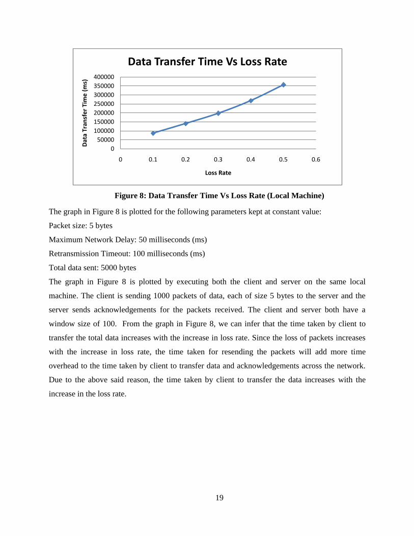
Figure 8: Data Transfer Time Vs Loss Rate (Local Machine)

The graph in Figure 8 is plotted for the following parameters kept at constant value:

Packet size: 5 bytes

Maximum Network Delay: 50 milliseconds (ms)

Retransmission Timeout: 100 milliseconds (ms)

Total data sent: 5000 bytes

The graph in Figure 8 is plotted by executing both the client and server on the same local

machine. The client is sending 1000 packets of data, each of size 5 bytes to the server and the

server sends acknowledgements for the packets received. The client and server both have a

window size of 100. From the graph in Figure 8, we can infer that the time taken by client to

transfer the total data increases with the increase in loss rate. Since the loss of packets increases

with the increase in loss rate, the time taken for resending the packets will add more time

overhead to the time taken by client to transfer data and acknowledgements across the network.

Due to the above said reason, the time taken by client to transfer the data increases with the

increase in the loss rate.

0

50000

100000

150000

200000

250000

300000

350000

400000

0 0.1 0.2 0.3 0.4 0.5 0.6

Dat

a Tr

ansf

er

Tim

e (

ms)

Loss Rate

Data Transfer Time Vs Loss Rate

20

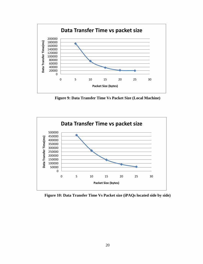
Figure 9: Data Transfer Time Vs Packet Size (Local Machine)

Figure 10: Data Transfer Time Vs Packet size (iPAQs located side by side)

020000400006000080000

100000120000140000160000180000200000

0 5 10 15 20 25 30

Dat

a Tr

ansf

er

Tim

e(m

s)

Packet Size (bytes)

Data Transfer Time vs packet size

050000

100000150000200000250000300000350000400000450000500000

0 5 10 15 20 25 30

Dat

a Tr

ansf

er

Tim

e(m

s)

Packet Size (bytes)


21

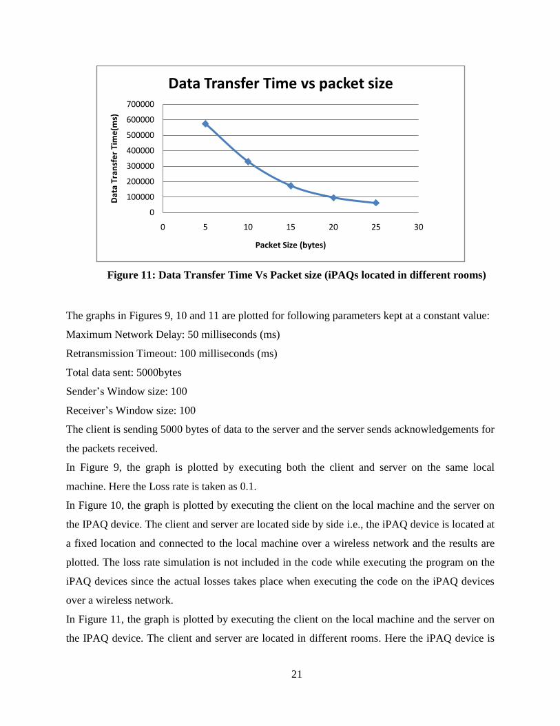
Figure 11: Data Transfer Time Vs Packet size (iPAQs located in different rooms)

The graphs in Figures 9, 10 and 11 are plotted for following parameters kept at a constant value:



Total data sent: 5000bytes

Sender’s Window size: 100

Receiver’s Window size: 100

The client is sending 5000 bytes of data to the server and the server sends acknowledgements for

the packets received.

In Figure 9, the graph is plotted by executing both the client and server on the same local

machine. Here the Loss rate is taken as 0.1.

In Figure 10, the graph is plotted by executing the client on the local machine and the server on

the IPAQ device. The client and server are located side by side i.e., the iPAQ device is located at

a fixed location and connected to the local machine over a wireless network and the results are

plotted. The loss rate simulation is not included in the code while executing the program on the

iPAQ devices since the actual losses takes place when executing the code on the iPAQ devices

over a wireless network.


the IPAQ device. The client and server are located in different rooms. Here the iPAQ device is

0

100000

200000

300000

400000

500000

600000

700000

0 5 10 15 20 25 30

Dat

a Tr

ansf

er

Tim

e(m

s)

Packet Size (bytes)


22

taken back and forth from the local machine and the results are plotted. The total number of

packets (including retransmitted packets) transferred when packet sizes are 25, 20, 15, 10 and 5

are 2174, 2685, 3364, 4239 and 5632 respectively. The number of packets received when packet

sizes are 25, 20, 15, 10 and 5 are 1033, 1401, 1845, 2379 and 3526 respectively. The loss

percentage when packet sizes are 25, 20, 15, 10 and 5 are 0.524, 0.478, 0.451, 0.438 and 0.373

respectively. The above behavior is due to the reason that there is more chance of packet with

more size to be lost in transmission than the packet with less size.

From the graphs in the Figures 9, 10 and 11, we can infer that the time taken by

client to transfer the total data decreases with the increase in packet size. If we increase the

packet size, more amounts of data can be transferred at a time and the number of packets to be

transferred also decreases. i.e., for 5000 bytes of data, if the packet size is 5, 1000 packets are

needed to transfer the data. If the packet size is increased to 10, total data can be sent in 500

packets. Hence the time taken to transfer 1000 packets is more when compared to the time taken

to transfer 500 packets. The graphs in Figures 9, 10 and 11 clearly illustrate the above behavior.

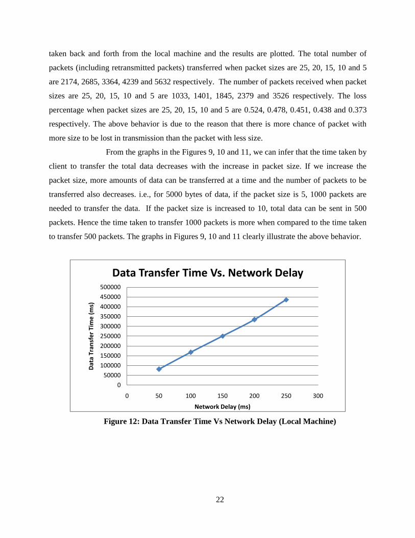
Figure 12: Data Transfer Time Vs Network Delay (Local Machine)

0

50000

100000

150000

200000

250000

300000

350000

400000

450000

500000

0 50 100 150 200 250 300

Dat

a Tr

ansf

er

Tim

e (

ms)

Network Delay (ms)

Data Transfer Time Vs. Network Delay

23

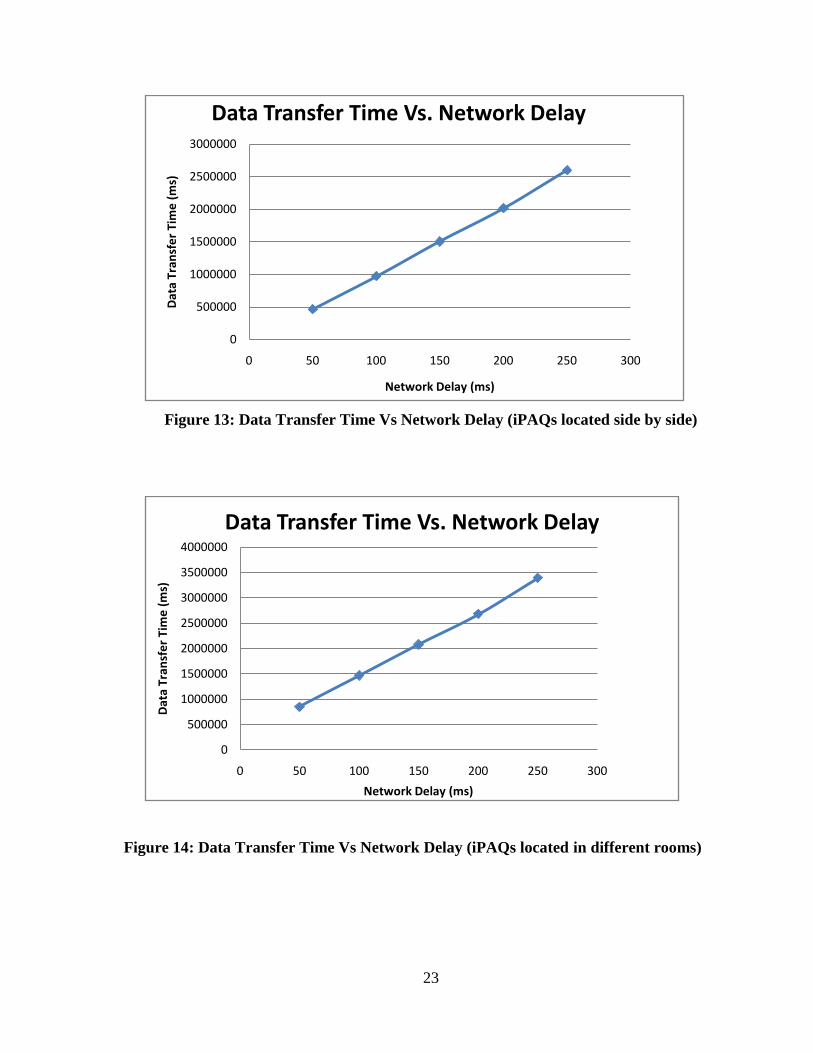
Figure 13: Data Transfer Time Vs Network Delay (iPAQs located side by side)

Figure 14: Data Transfer Time Vs Network Delay (iPAQs located in different rooms)

0

500000

1000000

1500000

2000000

2500000

3000000

0 50 100 150 200 250 300

Dat

a Tr

ansf

er

Tim

e (

ms)

Network Delay (ms)


0

500000

1000000

1500000

2000000

2500000

3000000

3500000

4000000

0 50 100 150 200 250 300

Dat

a Tr

ansf

er

Tim

e (

ms)

Network Delay (ms)


24

The graphs in Figures 12, 13 and 14 are plotted for following parameters kept at a constant

value:


Total data sent: 5000bytes



The client is sending 1000 packets of data, each packet of size 5 bytes to the server and the

server sends acknowledgements for the packets received. The Retransmission timeout is taken

double the value of network delay and the graphs are plotted.











taken back and forth from the local machine and the results are plotted.

From the graphs in the Figures 12, 13 and 14, we can infer that the time taken

by client to transfer data increases with the increase in network delay. This is due to the reason

that if we increase the network delay, the packets will be transferred at a slower rate and time

taken for the total data transfer will increase. The graphs in Figure 8, Figure 9 and Figure 10

clearly illustrate the above behavior.

25

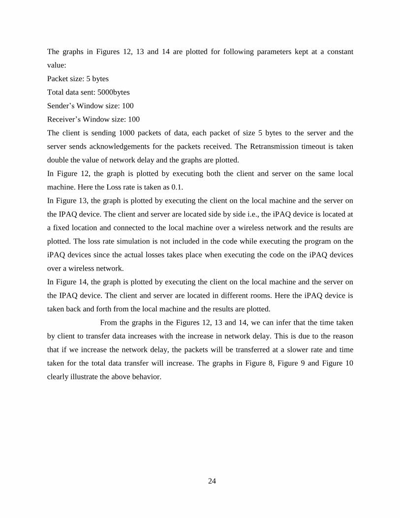
Figure 15: Data Transfer Time Vs Total Data sent (Local Machine)

Figure 16: Data Transfer Time Vs Total Data sent (iPAQs located side by side)

0

10000

20000

30000

40000

50000

60000

70000

80000

90000

0 2000 4000 6000 8000 10000 12000

Dat

a Tr

ansf

er

Tim

e (

ms)

Total Data sent (bytes)

Data Transfer Time vs Total data sent

0

100000

200000

300000

400000

500000

600000

0 2000 4000 6000 8000 10000 12000

Dat

a Tr

ansf

er

Tim

e (

ms)

Total data sent (bytes)


26

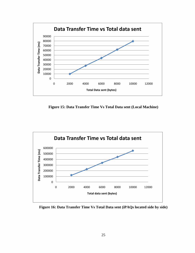
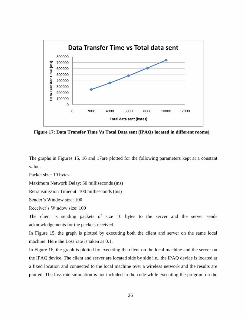
Figure 17: Data Transfer Time Vs Total Data sent (iPAQs located in different rooms)

The graphs in Figures 15, 16 and 17are plotted for the following parameters kept at a constant

value:






The client is sending packets of size 10 bytes to the server and the server sends

acknowledgements for the packets received.







0

100000

200000

300000

400000

500000

600000

700000

800000

0 2000 4000 6000 8000 10000 12000

Dat

a Tr

ansf

er

Tim

e (

ms)



27





taken back and forth from the local machine and the results are plotted.

From the graphs in Figures 15, 16 and 17, we can infer that the time taken by

client to transfer data increases with the increase in total amount of data transferred. This is due

to the reason that if we increase the amount of data that is to be transferred, more number of

packets needs to be transferred. i.e., for 2000 bytes of data, if the packet size is 10 bytes, 200

packets are needed to transfer the data and for 10000 bytes of data, if the packet size is 10 bytes,

1000 packets are needed to transfer the data. Hence the time taken to transfer 1000 packets is

more when compared to the time taken to transfer 200 packets. The graphs in in Figures 15, 16

and 17 clearly illustrate the above behavior.

The time taken for the client to transfer the total data in the graphs in Figures 9,

12 and 15 is less when compared to the time taken by the client to transfer the total data in the

graph in Figure 10, 13 and 16 respectively. This is due to the reason that there is more chance of

packet losses in the case of executing the protocol on iPAQ devices when compared to executing

the protocol on the local machine and the lost packets need to be retransmitted, which adds more

time overhead for the total data transfer time. The time taken for the client to transfer the total

data in the graphs in Figures 10, 13 and 16 is less when compared to the time taken by the client

to transfer the total data in the graph in Figure 11, 14 and 17. This is due to the reason that there

is more chance of packet losses in the case where iPAQ device is located in different room when

compared to the case where iPAQ is located side by side to the local machine and the lost

packets need to be retransmitted, which adds more time overhead for the total data transfer time.

28

Figure 18: Time gap between packets sent Vs Rate (# received packets / # sent packet)


0

0.2

0.4

0.6

0.8

1

1.2

0 2 4 6 8 10 12 14

Rat

e=(

# re

ceiv

ed

pac

ket/

# se

nt

pac

ket)

Time gap between packets sent (milli seconds)

Time gap between packets sent Vs. Rate

0

0.2

0.4

0.6

0.8

1

1.2

0 2 4 6 8 10 12 14

Rat

e=(

# re

ceiv

ed

pac

ket/

# se

nt

pac

ket)



29



0

0.2

0.4

0.6

0.8

1

1.2

0 2 4 6 8 10 12 14

Rat

e=(

# re

ceiv

ed

pac

ket/

# se

nt

pac

ket)



0.910.920.930.940.950.960.970.980.99

11.01

0 2 4 6 8 10 12 14

Rat

e=(

# re

ceiv

ed

pac

ket/

# se

nt

pac

ket)



30

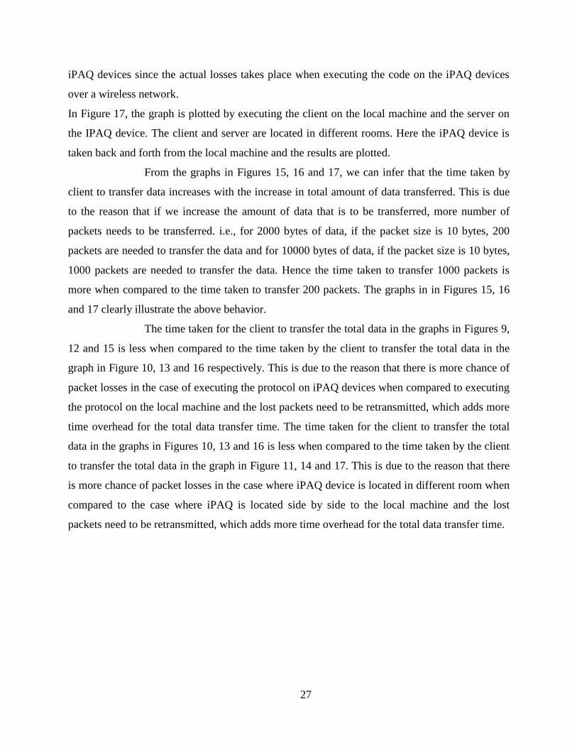
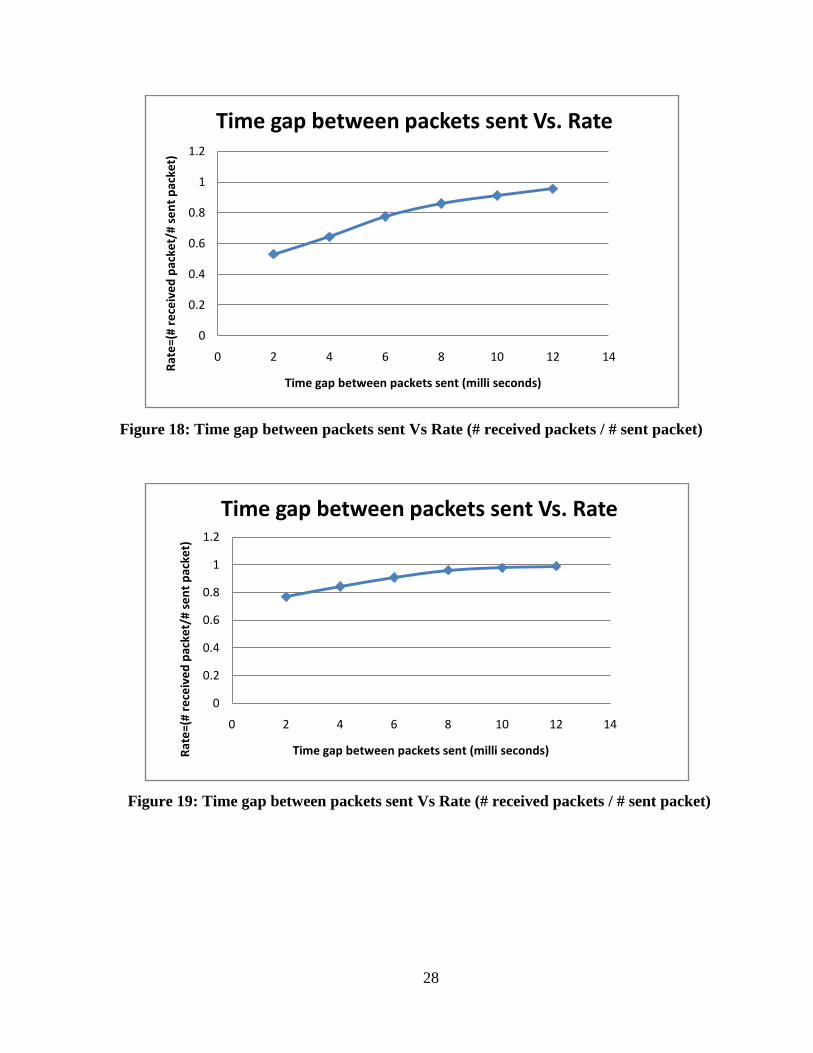
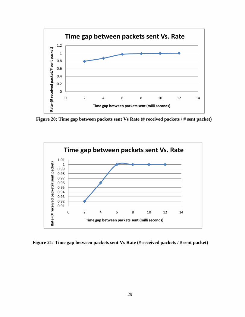
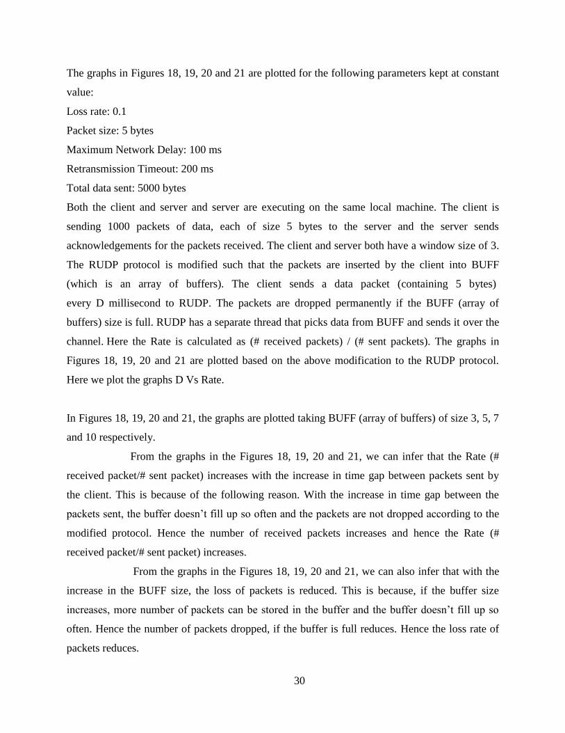
The graphs in Figures 18, 19, 20 and 21 are plotted for the following parameters kept at constant

value:

Loss rate: 0.1


Maximum Network Delay: 100 ms

Retransmission Timeout: 200 ms


Both the client and server and server are executing on the same local machine. The client is

sending 1000 packets of data, each of size 5 bytes to the server and the server sends

acknowledgements for the packets received. The client and server both have a window size of 3.

The RUDP protocol is modified such that the packets are inserted by the client into BUFF

(which is an array of buffers). The client sends a data packet (containing 5 bytes)

every D millisecond to RUDP. The packets are dropped permanently if the BUFF (array of

buffers) size is full. RUDP has a separate thread that picks data from BUFF and sends it over the

channel. Here the Rate is calculated as (# received packets) / (# sent packets). The graphs in

Figures 18, 19, 20 and 21 are plotted based on the above modification to the RUDP protocol.

Here we plot the graphs D Vs Rate.

In Figures 18, 19, 20 and 21, the graphs are plotted taking BUFF (array of buffers) of size 3, 5, 7

and 10 respectively.

From the graphs in the Figures 18, 19, 20 and 21, we can infer that the Rate (#

received packet/# sent packet) increases with the increase in time gap between packets sent by

the client. This is because of the following reason. With the increase in time gap between the

packets sent, the buffer doesn’t fill up so often and the packets are not dropped according to the

modified protocol. Hence the number of received packets increases and hence the Rate (#

received packet/# sent packet) increases.

From the graphs in the Figures 18, 19, 20 and 21, we can also infer that with the

increase in the BUFF size, the loss of packets is reduced. This is because, if the buffer size

increases, more number of packets can be stored in the buffer and the buffer doesn’t fill up so

often. Hence the number of packets dropped, if the buffer is full reduces. Hence the loss rate of

packets reduces.

31



00.10.20.30.40.50.60.70.80.9

1

0 2 4 6 8 10 12 14Rat

e=(

# re

ceiv

ed

pac

ket/

# se

nt

pac

ket)



0

0.2

0.4

0.6

0.8

1

1.2

0 2 4 6 8 10 12 14Rat

e=(

# re

ceiv

ed

pac

ket/

# se

nt

pac

ket)



32



0

0.2

0.4

0.6

0.8

1

1.2

0 2 4 6 8 10 12 14

Rat

e=(

# re

ceiv

ed

pac

ket/

# se

nt

pac

ket)



0

0.2

0.4

0.6

0.8

1

1.2

0 2 4 6 8 10 12 14

Rat

e=(

# re

ceiv

ed

pac

ket/

# se

nt

pac

ket)



33

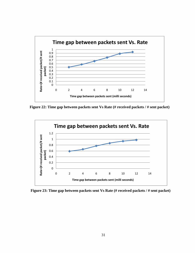
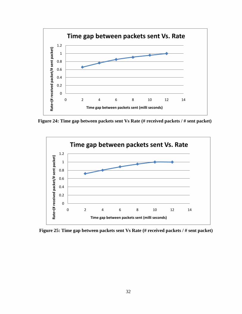
The graphs in Figures 22, 23, 24 and 25 are plotted for the following parameters kept at constant

value:


Maximum Network Delay: 100 ms

Retransmission Timeout: 200 ms


Here the client is executing on the iPAQ device and the server is executing on the local machine.

The client is sending 1000 packets of data, each of size 5 bytes to the server and the server sends

acknowledgements for the packets received. The client and server both have a window size of 3.

The RUDP protocol is modified such that the packets are inserted by the client into BUFF

(which is an array of buffers). The client sends a data packet (containing 5 bytes)

every D millisecond to RUDP. The packets are dropped permanently if the BUFF (array of

buffers) size is full. RUDP has a separate thread that picks data from BUFF and sends it over the

channel. Here the Rate is calculated as (# received packets) / (# sent packets). The graphs in

Figures 22, 23, 24 and 25 are plotted based on the above modification to the RUDP protocol.

Here we plot the graphs D vs. Rate.

In Figures 22, 23, 24 and 25, the graphs are plotted taking BUFF (array of buffers) of size 3, 5, 7

and 10 respectively.

From the graphs in the Figures 22, 23, 24 and 25, we can infer that the Rate (#

received packet/# sent packet) increases with the increase in time gap between packets sent by

the client. This is because of the following reason. With the increase in time gap between the

packets sent, the buffer doesn’t fill up so often and the packets are not dropped according to the

modified protocol. Hence the number of received packets increases and hence the Rate (#

received packet/# sent packet) increases.

From the graphs in the Figures 22, 23, 24 and 25, we can also infer that with the

increase in the BUFF size, the loss of packets is reduced. This is because, if the buffer size

increases, more number of packets can be stored in the buffer and the buffer doesn’t fill up so

often. Hence the number of packets dropped, if the buffer is full reduces.

When the results on the iPAQ devices compared to the local machine, the loss

rate of packets is more when protocol is executing on iPAQs. This is because the actual losses of

packets also come into account along with the packets dropped if the buffer is full.

34

Figure 26: Data Transfer Time Vs Buffer Utilization (Local Machine)

Figure 27: Data Transfer Time Vs Buffer Utilization (iPAQ devices)

0

20

40

60

80

100

120

0 2000 4000 6000 8000 10000 12000

Nu

mb

er

of

bu

ffe

rs u

sed

Data Transfer Time (ms)

Data Transfer Time Vs Buffer Utilization

0

20

40

60

80

100

120

0 2000 4000 6000 8000 10000 12000 14000

Nu

mb

er

of

bu

ffe

rs u

sed

Data Transfer Time (ms)

Data Transfer Time Vs Buffer Utilization

35

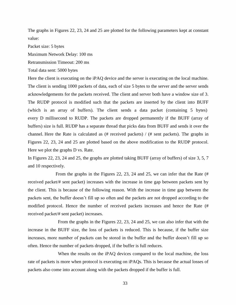
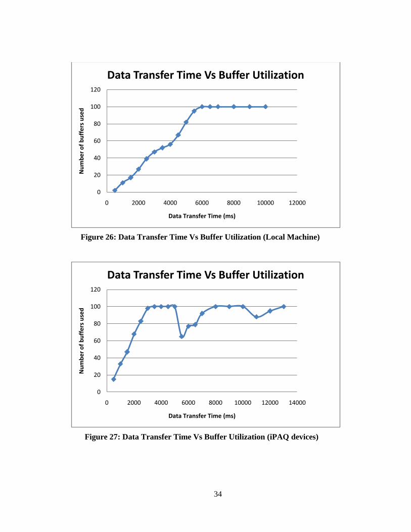
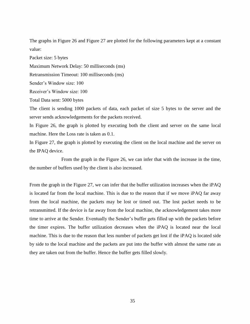
The graphs in Figure 26 and Figure 27 are plotted for the following parameters kept at a constant

value:






Total Data sent: 5000 bytes

The client is sending 1000 packets of data, each packet of size 5 bytes to the server and the

server sends acknowledgements for the packets received.




the IPAQ device.

From the graph in the Figure 26, we can infer that with the increase in the time,

the number of buffers used by the client is also increased.

From the graph in the Figure 27, we can infer that the buffer utilization increases when the iPAQ

is located far from the local machine. This is due to the reason that if we move iPAQ far away

from the local machine, the packets may be lost or timed out. The lost packet needs to be

retransmitted. If the device is far away from the local machine, the acknowledgement takes more

time to arrive at the Sender. Eventually the Sender’s buffer gets filled up with the packets before

the timer expires. The buffer utilization decreases when the iPAQ is located near the local

machine. This is due to the reason that less number of packets get lost if the iPAQ is located side

by side to the local machine and the packets are put into the buffer with almost the same rate as

they are taken out from the buffer. Hence the buffer gets filled slowly.

36

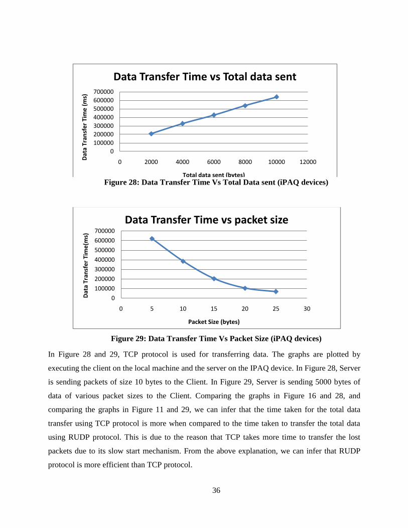
Figure 28: Data Transfer Time Vs Total Data sent (iPAQ devices)

Figure 29: Data Transfer Time Vs Packet Size (iPAQ devices)

In Figure 28 and 29, TCP protocol is used for transferring data. The graphs are plotted by

executing the client on the local machine and the server on the IPAQ device. In Figure 28, Server

is sending packets of size 10 bytes to the Client. In Figure 29, Server is sending 5000 bytes of

data of various packet sizes to the Client. Comparing the graphs in Figure 16 and 28, and

comparing the graphs in Figure 11 and 29, we can infer that the time taken for the total data

transfer using TCP protocol is more when compared to the time taken to transfer the total data

using RUDP protocol. This is due to the reason that TCP takes more time to transfer the lost

packets due to its slow start mechanism. From the above explanation, we can infer that RUDP

protocol is more efficient than TCP protocol.

0

100000

200000

300000

400000

500000

600000

700000

0 2000 4000 6000 8000 10000 12000

Dat

a Tr

ansf

er

Tim

e (

ms)



0

100000

200000

300000

400000

500000

600000

700000

0 5 10 15 20 25 30

Dat

a Tr

ansf

er

Tim

e(m

s)

Packet Size (bytes)


37

CHAPTER 5: CONCLUSION AND FUTURE WORK

The architecture, implementation and performance of Reliable UDP protocol is discussed in this

report. As UDP is an unreliable protocol, Reliable UDP protocol is used for reliable

communication. Reliable UDP protocol is implemented using the sliding window protocols.

Among the sliding window protocols, Selective Repeat protocol is used for implementing the

RUDP protocol since it is an efficient and performance effective protocol [2]. The performance

results of RUDP protocol show the guaranteed-order packet delivery and efficiency of the

protocol. The performance results of RUDP protocol on windows mobile devices (HP IPAQS)

show the reliable delivery of packets up to a maximum number of retransmissions. The protocol

is capable to deliver large data over high speed networks when the packet is of acceptable size.

Processing and memory overhead comes along with the additional complexity of the

Selective Repeat protocol, which is its main drawback. As a future work, one can implement

congestion control mechanism to overcome the processing and memory overhead. In this

protocol, security of the data transferred is not considered. Providing security can also be one of

the future works that can be done.

http://en.wikipedia.org/wiki/Packet_(information_technology)

38

CHAPTER 6: REFERENCES

[1] Andrew S. Tanenbaum. Computer Networks, Third Edition.

[2] Ian F. Akyildiz and Wei Liu (1991). A General Analysis Technique for ARQ Protocol

performance in high speed networks. In INFOCOM ‘91 Proceedings, Tenth Annual Joint

Conference of the IEEE Computer and Communications Societies, Bal Harbour, FL, USA.

[3] Hemant Sengar, Haining Wang, Duminda Wijesekera and Sushil Jajodia (2006). Fast

Detection of Denial-of-Service Attacks on IP Telephony. In Quality of Service ‘06.

IWQoS ‘06. 14th IEEE International Workshop, New Haven, CT.

[4] Toshio Soumiya, Koji Kamichi and Arnold Brag (1999). Performance evaluation of TCP

over ATM World Wide Web Traffic. In ATM Workshop ‘99. IEEE Proceedings, Kochi,

Japan.

RELIABLE USER DATAGRAM PROTOCOL (RUDP) by ABHILASH ...

Documents

Transcript of RELIABLE USER DATAGRAM PROTOCOL (RUDP) by ABHILASH ...