Reliable Massively Parallel Symbolic Computing:Fault Tolerance for a Distributed Haskell

by

Robert Stewart

Submitted in conformity with the requirementsfor the degree of Doctor of Philosophy

Heriot Watt University

School of Mathematical and Computer Sciences

Submitted November, 2013

The copyright in this thesis is owned by the author. Any quotation from this thesis or use ofany of the information contained in it must acknowledge this thesis as the source of the

quotation or information.

Abstract

As the number of cores in manycore systems grows exponentially, the number of failures isalso predicted to grow exponentially. Hence massively parallel computations must be able totolerate faults. Moreover new approaches to language design and system architecture are neededto address the resilience of massively parallel heterogeneous architectures.

Symbolic computation has underpinned key advances in Mathematics and Computer Sci-ence, for example in number theory, cryptography, and coding theory. Computer algebra soft-ware systems facilitate symbolic mathematics. Developing these at scale has its own distinctiveset of challenges, as symbolic algorithms tend to employ complex irregular data and controlstructures. SymGridParII is a middleware for parallel symbolic computing on massively parallelHigh Performance Computing platforms. A key element of SymGridParII is a domain specificlanguage (DSL) called Haskell Distributed Parallel Haskell (HdpH). It is explicitly designed forscalable distributed-memory parallelism, and employs work stealing to load balance dynamicallygenerated irregular task sizes.

To investigate providing scalable fault tolerant symbolic computation we design, implementand evaluate a reliable version of HdpH, HdpH-RS. Its reliable scheduler detects and handlesfaults, using task replication as a key recovery strategy. The scheduler supports load balancingwith a fault tolerant work stealing protocol. The reliable scheduler is invoked with two faulttolerance primitives for implicit and explicit work placement, and 10 fault tolerant parallelskeletons that encapsulate common parallel programming patterns. The user is oblivious tomany failures, they are instead handled by the scheduler.

An operational semantics describes small-step reductions on states. A simple abstract ma-chine for scheduling transitions and task evaluation is presented. It defines the semantics ofsupervised futures, and the transition rules for recovering tasks in the presence of failure. Thetransition rules are demonstrated with a fault-free execution, and three executions that recoverfrom faults.

The fault tolerant work stealing has been abstracted in to a Promela model. The SPINmodel checker is used to exhaustively search the intersection of states in this automaton tovalidate a key resiliency property of the protocol. It asserts that an initially empty supervisedfuture on the supervisor node will eventually be full in the presence of all possible combinationsof failures.

The performance of HdpH-RS is measured using five benchmarks. Supervised schedulingachieves a speedup of 757 with explicit task placement and 340 with lazy work stealing whenexecuting Summatory Liouville up to 1400 cores of a HPC architecture. Moreover, supervisionoverheads are consistently low scaling up to 1400 cores. Low recovery overheads are observed inthe presence of frequent failure when lazy on-demand work stealing is used. A Chaos Monkeymechanism has been developed for stress testing resiliency with random failure combinations.All unit tests pass in the presence of random failure, terminating with the expected results.

2

Dedication

To Mum and Dad.

3

Acknowledgements

Foremost, I would like to express my deepest thanks to my two supervisors, Professor PhilTrinder and Dr Patrick Maier. Their patience, encouragement, and immense knowledgewere key motivations throughout my PhD. They carry out their research with an objectiveand principled approach to computer science. They persuasively conveyed an interest inmy work, and I am grateful for my inclusion in their HPC-GAP project.

Phil has been my supervisor and guiding beacon through four years of computerscience MEng and PhD research. I am truly thankful for his steadfast integrity, andselfless dedication to both my personal and academic development. I cannot think of abetter supervisor to have. Patrick is a mentor and friend, from whom I have learnt thevital skill of disciplined critical thinking. His forensic scrutiny of my technical writinghas been invaluable. He has always found the time to propose consistently excellentimprovements. I owe a great debt of gratitude to Phil and Patrick.

I would like to thank Professor Greg Michaelson for offering thorough and excellentfeedback on an earlier version of this thesis. In addition, a thank you to Dr GudmundGrov. Gudmund gave feedback on Chapter 4 of this thesis, and suggested generalityimprovements to my model checking abstraction of HdpH-RS.

A special mention for Dr Edsko de Vries of Well Typed, for our insightful and detaileddiscussions about network transport design. Furthermore, Edsko engineered the networkabstraction layer on which the fault detecting component of HdpH-RS is built.

I thank the computing officers at Heriot-Watt University and the Edinburgh ParallelComputing Centre for their support and hardware access for the performance evaluationof HdpH-RS.

4

Contents

1 Introduction 101.1 Context . . . . . . . . . . . . . . . . . . . . . . . . . . . . . . . . . . . . 101.2 Contributions . . . . . . . . . . . . . . . . . . . . . . . . . . . . . . . . . 111.3 Authorship & Collaboration . . . . . . . . . . . . . . . . . . . . . . . . . 13

1.3.1 Authorship . . . . . . . . . . . . . . . . . . . . . . . . . . . . . . 131.3.2 Collaboration . . . . . . . . . . . . . . . . . . . . . . . . . . . . . 14

2 Related Work 162.1 Dependability of Distributed Systems . . . . . . . . . . . . . . . . . . . . 16

2.1.1 Distributed Systems Terminology . . . . . . . . . . . . . . . . . . 172.1.2 Dependable Systems . . . . . . . . . . . . . . . . . . . . . . . . . 17

2.2 Fault Tolerance . . . . . . . . . . . . . . . . . . . . . . . . . . . . . . . . 182.2.1 Fault Tolerance Terminology . . . . . . . . . . . . . . . . . . . . . 182.2.2 Failure Rates . . . . . . . . . . . . . . . . . . . . . . . . . . . . . 202.2.3 Fault Tolerance Mechanisms . . . . . . . . . . . . . . . . . . . . . 222.2.4 Software Based Fault Tolerance . . . . . . . . . . . . . . . . . . . 25

2.3 Classifications of Fault Tolerance Implementations . . . . . . . . . . . . . 272.3.1 Fault Tolerance for DOTS Middleware . . . . . . . . . . . . . . . 272.3.2 MapReduce . . . . . . . . . . . . . . . . . . . . . . . . . . . . . . 282.3.3 Distributed Datastores . . . . . . . . . . . . . . . . . . . . . . . . 282.3.4 Fault Tolerant Networking Protocols . . . . . . . . . . . . . . . . 292.3.5 Fault Tolerant MPI . . . . . . . . . . . . . . . . . . . . . . . . . . 302.3.6 Erlang . . . . . . . . . . . . . . . . . . . . . . . . . . . . . . . . . 322.3.7 Process Supervision in Erlang OTP . . . . . . . . . . . . . . . . . 33

2.4 CloudHaskell . . . . . . . . . . . . . . . . . . . . . . . . . . . . . . . . . 342.4.1 Fault Tolerance in CloudHaskell . . . . . . . . . . . . . . . . . . . 342.4.2 CloudHaskell 2.0 . . . . . . . . . . . . . . . . . . . . . . . . . . . 35

2.5 SymGridParII . . . . . . . . . . . . . . . . . . . . . . . . . . . . . . . . . 36

5

2.6 HdpH . . . . . . . . . . . . . . . . . . . . . . . . . . . . . . . . . . . . . 362.6.1 HdpH Language Design . . . . . . . . . . . . . . . . . . . . . . . 362.6.2 HdpH Primitives . . . . . . . . . . . . . . . . . . . . . . . . . . . 372.6.3 Programming Example with HdpH . . . . . . . . . . . . . . . . . 372.6.4 HdpH Implementation . . . . . . . . . . . . . . . . . . . . . . . . 38

2.7 Fault Tolerance Potential for HdpH . . . . . . . . . . . . . . . . . . . . . 38

3 Designing a Fault Tolerant Programming Language for DistributedMemory Scheduling 413.1 Supervised Workpools Prototype . . . . . . . . . . . . . . . . . . . . . . 423.2 Introducing Work Stealing Scheduling . . . . . . . . . . . . . . . . . . . . 433.3 Reliable Scheduling for Fault Tolerance . . . . . . . . . . . . . . . . . . . 45

3.3.1 HdpH-RS Terminology . . . . . . . . . . . . . . . . . . . . . . . . 453.3.2 HdpH-RS Programming Primitives . . . . . . . . . . . . . . . . . 47

3.4 Operational Semantics . . . . . . . . . . . . . . . . . . . . . . . . . . . . 483.4.1 Semantics of the Host Language . . . . . . . . . . . . . . . . . . . 493.4.2 HdpH-RS Core Syntax . . . . . . . . . . . . . . . . . . . . . . . . 493.4.3 Small Step Operational Semantics . . . . . . . . . . . . . . . . . . 503.4.4 Execution of Transition Rules . . . . . . . . . . . . . . . . . . . . 58

3.5 Designing a Fault Tolerant Scheduler . . . . . . . . . . . . . . . . . . . . 623.5.1 Work Stealing Protocol . . . . . . . . . . . . . . . . . . . . . . . . 623.5.2 Task Locality . . . . . . . . . . . . . . . . . . . . . . . . . . . . . 643.5.3 Duplicate Sparks . . . . . . . . . . . . . . . . . . . . . . . . . . . 683.5.4 Fault Tolerant Scheduling Algorithm . . . . . . . . . . . . . . . . 713.5.5 Fault Recovery Examples . . . . . . . . . . . . . . . . . . . . . . . 75

3.6 Summary . . . . . . . . . . . . . . . . . . . . . . . . . . . . . . . . . . . 80

4 The Validation of Reliable Distributed Scheduling for HdpH-RS 814.1 Modeling Asynchronous Environments . . . . . . . . . . . . . . . . . . . 82

4.1.1 Asynchronous Message Passing . . . . . . . . . . . . . . . . . . . 824.1.2 Asynchronous Work Stealing . . . . . . . . . . . . . . . . . . . . . 83

4.2 Promela Model of Fault Tolerant Scheduling . . . . . . . . . . . . . . . . 844.2.1 Introduction to Promela . . . . . . . . . . . . . . . . . . . . . . . 844.2.2 Key Reliable Scheduling Properties . . . . . . . . . . . . . . . . . 854.2.3 HdpH-RS Abstraction . . . . . . . . . . . . . . . . . . . . . . . . 864.2.4 Out-of-Scope Characteristics . . . . . . . . . . . . . . . . . . . . . 88

4.3 Scheduling Model . . . . . . . . . . . . . . . . . . . . . . . . . . . . . . . 88

6

4.3.1 Channels & Nodes . . . . . . . . . . . . . . . . . . . . . . . . . . 884.3.2 Node Failure . . . . . . . . . . . . . . . . . . . . . . . . . . . . . 914.3.3 Node State . . . . . . . . . . . . . . . . . . . . . . . . . . . . . . 924.3.4 Spark Location Tracking . . . . . . . . . . . . . . . . . . . . . . . 944.3.5 Message Handling . . . . . . . . . . . . . . . . . . . . . . . . . . . 95

4.4 Verifying Scheduling Properties . . . . . . . . . . . . . . . . . . . . . . . 1034.4.1 Linear Temporal Logic & Propositional Symbols . . . . . . . . . . 1034.4.2 Verification Options & Model Checking Platform . . . . . . . . . 104

4.5 Model Checking Results . . . . . . . . . . . . . . . . . . . . . . . . . . . 1054.5.1 Counter Property . . . . . . . . . . . . . . . . . . . . . . . . . . . 1064.5.2 Desirable Properties . . . . . . . . . . . . . . . . . . . . . . . . . 106

4.6 Identifying Scheduling Bugs . . . . . . . . . . . . . . . . . . . . . . . . . 107

5 Implementing a Fault Tolerant Programming Language and ReliableScheduler 1095.1 HdpH-RS Architecture . . . . . . . . . . . . . . . . . . . . . . . . . . . . 109

5.1.1 Implementing Futures . . . . . . . . . . . . . . . . . . . . . . . . 1115.1.2 Guard Posts . . . . . . . . . . . . . . . . . . . . . . . . . . . . . . 116

5.2 HdpH-RS Primitives . . . . . . . . . . . . . . . . . . . . . . . . . . . . . 1175.3 Recovering Supervised Sparks and Threads . . . . . . . . . . . . . . . . . 1185.4 HdpH-RS Node State . . . . . . . . . . . . . . . . . . . . . . . . . . . . . 120

5.4.1 Communication State . . . . . . . . . . . . . . . . . . . . . . . . . 1205.4.2 Sparkpool State . . . . . . . . . . . . . . . . . . . . . . . . . . . . 1215.4.3 Threadpool State . . . . . . . . . . . . . . . . . . . . . . . . . . . 122

5.5 Fault Detecting Communications Layer . . . . . . . . . . . . . . . . . . . 1235.5.1 Distributed Virtual Machine . . . . . . . . . . . . . . . . . . . . . 1235.5.2 Message Passing API . . . . . . . . . . . . . . . . . . . . . . . . . 1235.5.3 RTS Messages . . . . . . . . . . . . . . . . . . . . . . . . . . . . . 1245.5.4 Detecting Node Failure . . . . . . . . . . . . . . . . . . . . . . . . 125

5.6 Comparison with Other Fault Tolerant Language Implementations . . . . 1295.6.1 Erlang . . . . . . . . . . . . . . . . . . . . . . . . . . . . . . . . . 1295.6.2 Hadoop . . . . . . . . . . . . . . . . . . . . . . . . . . . . . . . . 1305.6.3 GdH Fault Tolerance Design . . . . . . . . . . . . . . . . . . . . . 1315.6.4 Fault Tolerant MPI Implementations . . . . . . . . . . . . . . . . 132

6 Fault Tolerant Programming & Reliable Scheduling Evaluation 1336.1 Fault Tolerant Programming with HdpH-RS . . . . . . . . . . . . . . . . 134

7

6.1.1 Programming With HdpH-RS Fault Tolerance Primitives . . . . . 1346.1.2 Fault Tolerant Parallel Skeletons . . . . . . . . . . . . . . . . . . 1346.1.3 Programming With Fault Tolerant Skeletons . . . . . . . . . . . . 137

6.2 Launching Distributed Programs . . . . . . . . . . . . . . . . . . . . . . 1386.3 Measurements Platform . . . . . . . . . . . . . . . . . . . . . . . . . . . 141

6.3.1 Benchmarks . . . . . . . . . . . . . . . . . . . . . . . . . . . . . . 1416.3.2 Measurement Methodologies . . . . . . . . . . . . . . . . . . . . . 1426.3.3 Hardware Platforms . . . . . . . . . . . . . . . . . . . . . . . . . 142

6.4 Performance With No Failure . . . . . . . . . . . . . . . . . . . . . . . . 1436.4.1 HdpH Scheduler Performance . . . . . . . . . . . . . . . . . . . . 1436.4.2 Runtime & Speed Up . . . . . . . . . . . . . . . . . . . . . . . . . 145

6.5 Performance With Recovery . . . . . . . . . . . . . . . . . . . . . . . . . 1506.5.1 Simultaneous Multiple Failures . . . . . . . . . . . . . . . . . . . 1506.5.2 Chaos Monkey . . . . . . . . . . . . . . . . . . . . . . . . . . . . 1536.5.3 Increasing Recovery Overheads with Eager Scheduling . . . . . . 156

6.6 Evaluation Discussion . . . . . . . . . . . . . . . . . . . . . . . . . . . . . 159

7 Conclusion 1627.1 Summary . . . . . . . . . . . . . . . . . . . . . . . . . . . . . . . . . . . 1627.2 Limitations . . . . . . . . . . . . . . . . . . . . . . . . . . . . . . . . . . 1657.3 Future Work . . . . . . . . . . . . . . . . . . . . . . . . . . . . . . . . . . 165

A Appendix 188A.1 Supervised Workpools . . . . . . . . . . . . . . . . . . . . . . . . . . . . 188

A.1.1 Design of the Workpool . . . . . . . . . . . . . . . . . . . . . . . 189A.1.2 Use Case Scenarios . . . . . . . . . . . . . . . . . . . . . . . . . . 191A.1.3 Workpool Implementation . . . . . . . . . . . . . . . . . . . . . . 192A.1.4 Workpool Scheduling . . . . . . . . . . . . . . . . . . . . . . . . . 196A.1.5 Workpool High Level Fault Tolerant Abstractions . . . . . . . . . 196A.1.6 Supervised Workpool Evaluation . . . . . . . . . . . . . . . . . . 198A.1.7 Summary . . . . . . . . . . . . . . . . . . . . . . . . . . . . . . . 203

A.2 Programming with Futures . . . . . . . . . . . . . . . . . . . . . . . . . . 203A.2.1 Library Support for Distributed Functional Futures . . . . . . . . 203A.2.2 Primitive Names for Future Operations . . . . . . . . . . . . . . . 204

A.3 Promela Model Implementation . . . . . . . . . . . . . . . . . . . . . . . 207A.4 Feeding Promela Bug Fix to Implementation . . . . . . . . . . . . . . . . 212

A.4.1 Bug Fix in Promela Model . . . . . . . . . . . . . . . . . . . . . . 212

8

A.4.2 Bug Fix in Haskell . . . . . . . . . . . . . . . . . . . . . . . . . . 212A.5 Network Transport Event Error Codes . . . . . . . . . . . . . . . . . . . 213A.6 Handling Dead Node Notifications . . . . . . . . . . . . . . . . . . . . . . 214A.7 Replicating Sparks and Threads . . . . . . . . . . . . . . . . . . . . . . . 215A.8 Propagating Failures from Transport Layer . . . . . . . . . . . . . . . . . 216A.9 HdpH-RS Skeleton API . . . . . . . . . . . . . . . . . . . . . . . . . . . . 217A.10 Using Chaos Monkey in Unit Testing . . . . . . . . . . . . . . . . . . . . 219A.11 Benchmark Implementations . . . . . . . . . . . . . . . . . . . . . . . . . 220

A.11.1 Fibonacci . . . . . . . . . . . . . . . . . . . . . . . . . . . . . . . 220A.11.2 Sum Euler . . . . . . . . . . . . . . . . . . . . . . . . . . . . . . . 221A.11.3 Summatory Liouville . . . . . . . . . . . . . . . . . . . . . . . . . 221A.11.4 Queens . . . . . . . . . . . . . . . . . . . . . . . . . . . . . . . . . 223A.11.5 Mandelbrot . . . . . . . . . . . . . . . . . . . . . . . . . . . . . . 225

9

Chapter 1

Introduction

1.1 Context

The manycore revolution is steadily increasing the performance and size of massively par-allel systems, to the point where system reliability becomes a pressing concern. Therefore,massively parallel compute jobs must be able to tolerate failures. Research in to HighPerformance Computing (HPC) spans many areas including language design and imple-mentation, low latency network protocols and parallel hardware. Popular languages forwriting HPC applications include Fortran or C with the Message Passing Interface (MPI).New approaches to language design and system architecture are needed to address thegrowing issue of massively parallel heterogeneous architectures, where processing capa-bility is non-uniform and failure is increasingly common.

Symbolic computation has underpinned key advances in Mathematics and ComputerScience. Developing computer algebra systems at scale has its own distinctive set ofchallenges, for example how to coordinate symbolic applications that exhibit highly ir-regular parallelism. The HPC-GAP project aims to coordinate symbolic computations inarchitectures with 106 cores [135]. At that scale, systems are heterogeneous and exhibitnon-uniform communication latency’s, and failures are a real issue. SymGridParII is amiddleware that has been designed for scaling computer algebra programs onto massivelyparallel HPC platforms [112].

A core element of SymGridParII is a domain specific language (DSL) called HaskellDistributed Parallel Haskell (HdpH). It supports both implicit and explicit parallelism.The design of HdpH was informed by the need for reliability, and the language has thepotential for fault tolerance. To investigate providing scalable fault tolerant symboliccomputation this thesis presents the design, implementation and evaluation of a ReliableScheduling version of HdpH, HdpH-RS. It adds two new fault tolerant primitives and 10

10

fault tolerant algorithmic skeletons. A reliable scheduler has been designed and imple-mented to support these primitives, and its operational semantics are given. The SPINmodel checker has been used to verify a key fault tolerance property of the underlyingwork stealing protocol.

1.2 Contributions

The thesis makes the following research contributions:

1. A critical review of fault tolerance in distributed systems. This coversexisting approaches to handling failures at various levels including fault tolerantcommunication layers, checkpointing and rollback, task and data replication, andfault tolerant algorithms (Chapter 2).

2. A supervised workpool as a software reliability mechanism [164]. The su-pervised fault tolerant workpool hides task scheduling, failure detection and taskreplication from the programmer. The fault detection and task replication tech-niques that support supervised workpools are prototypes for HdpH-RS mechanisms.Some benchmarks show low supervision overheads of between 2% and 7% in theabsence of faults. Increased runtimes are between 8% and 10%, attributed to failuredetection latency and task replication, when 1 node fails in a 10 node architecture(Appendix A.1).

3. The design of fault tolerant language HdpH extensions. The HdpH-RSprimitives supervisedSpawn and supervisedSpawnAt provide fault tolerance byinvoking supervised task scheduling. Their inception motivated the addition ofspawn and spawnAt to HdpH [113]. The APIs of the original and fault tolerantprimitives are identical, allowing the programmer to trivially opt-in to fault toler-ant scheduling (Section 3.3.2).

4. The design of a fault tolerant distributed scheduler. To support the HdpH-RS primitives, a fault tolerant scheduler has been developed. The reliable sched-uler algorithm is designed to support work stealing whilst tolerating random lossof single and simultaneous node failures. It supervises the location of supervisedtasks, using replication as a recovery technique. Task replication is restricted toexpressions with idempotent side effects i.e. side effects whose repetition cannot beobserved. Failures are encapsulated with isolated heaps for each HdpH-RS node, sothe loss of one node does not damage other nodes (Section 3.5).

11

5. An operational semantics for HdpH-RS. The operational semantics for HdpH-RS extends that of HdpH, providing small-step reduction on states of a simple ab-stract machine. They provide a concise and unambiguous description of the schedul-ing transitions in the absence and presence of failure, and the states of supervisedsparks and supervised futures. The transition rules are demonstrated with one fault-free execution, and three executions that recover and evaluate task replicas in thepresence of faults (Section 3.4).

6. A validation of the fault tolerant distributed scheduler with the SPINmodel checker. The work stealing scheduling algorithm is abstracted in to aPromela model and is formally verified with the SPIN model checker. Whilst themodel is an abstraction, it does model all failure combinations that may occurreal architectures on which HdpH-RS could be deployed. The abstraction has animmortal supervising node and three mortal thieving nodes competing for a sparkwith the work stealing protocol. Any node holding a task replica can write to afuture on the supervisor node. A key resiliency property of the model is expressedusing linear temporal logic, stipulating that the initially empty supervised futureon the supervisor node is eventually full despite node failures. The work stealingroutines on the supervisor and three thieves are translated in to a finite automaton.The SPIN model checker is used to exhaustively search the model’s state spaceto validate that the reliability property holds on all reachable states. This it doeshaving searched approximately 8.22 million states of the HdpH-RS fishing protocol,at a reachable depth of 124 transitions (Chapter 4).

7. The implementation of the HdpH-RS fault tolerant primitives and re-liable scheduler. The implementation of the spawn family of primitives and su-pervised futures are described. On top of the fault tolerant supervisedSpawn andsupervisedSpawnAt primitives, 10 algorithmic skeletons have been produced thatprovide high level fault tolerant parallel patterns of computation. All load-balancingand task recovery is hidden from the programmer. The fault tolerant spawn prim-itives honour the small-step operational semantics, and the reliable scheduler is animplementation of the verified Promela model. In extending HdpH, one module isadded for the fault tolerant strategies, and 14 modules are modified. This amountsto an additional 1271 lines of Haskell code in HdpH-RS, an increase of 52%. Theincrease is attributed to fault detection, fault recovery and task supervision code(Chapter 5).

8. An evaluation of fault tolerant scheduling performance. The fault tolerant

12

HdpH-RS primitives are used to implement five benchmarks. Runtimes and over-heads are reported, both in the presence and absence of faults. The benchmarksare executed on a 256 core Beowulf cluster [122] and on 1400 cores of HECToR[58], a national UK compute resource. The task supervision overheads are low atall scales up to 1400 cores. The scalability of the HdpH-RS scheduler design isdemonstrated on massively parallel architectures using both flat and hierarchicallynested supervision. Flat supervised scheduling achieves a speedup of 757 with ex-plicit task placement and 340 with lazy work stealing when executing SummatoryLiouville on HECToR using 1400 cores. Hierarchically nested supervised schedulingachieves a speedup of 89 with explicit task placement when executing Mandelbroton HECToR using 560 cores.

A Chaos Monkey failure injection mechanism [82] is built-in to the reliable schedulerto simulate random node loss. A suite of eight unit tests are used to assess theresilience of HdpH-RS. All unit tests pass in the presence of random failures onthe Beowulf cluster. Executions in the presence of random failure show that lazyon-demand scheduling is more suitable when failure is the common case, not theexception (Chapter 6).

9. Other contributions A new fault detecting transport layer has been implementedfor HdpH and HdpH-RS. This was collaborative work with members of the Haskellcommunity, including code and testing contributions of a new network transportAPI for distributed Haskells. (Section 5.5). In the domain of reliable distributedcomputing, two related papers were produced. The first [163] compares three highlevel MapReduce query languages for performance and expressivity. The other [162]compares the two programming models MapReduce and Fork/Join.

1.3 Authorship & Collaboration

1.3.1 Authorship

This thesis is closely based on the work reported in the following papers:

• Supervised Workpools for Reliable Massively Parallel Computing [164].Trends in Functional Programming, 13th International Symposium, TFP 2012, StAndrews, UK. Springer. With Phil Trinder and Patrick Maier. This paper presentsthe supervised workpool described in Appendix A.1. The fault detection and taskreplication techniques that support supervised workpools is a reliable computationprototype for HdpH-RS.

13

• Reliable Scalable Symbolic Computation: The Design of SymGridPar2[112]. 28th ACM Symposium On Applied Computing, SAC 2013, Coimbra, Portugal.ACM Press. With Phil Trinder and Patrick Maier. The author contributed the faultdetection, fault recovery and fault tolerant algorithmic skeleton designs for HdpH-RS. Supervision and recovery overheads for the Summatory Liouville applicationusing the supervised workpool were presented.

• Reliable Scalable Symbolic Computation: The Design of SymGridPar2[113]. Submitted to Computer Languages, Systems and Structures. Special Issue.Revised Selected Papers from 28th ACM Symposium On Applied Computing 2013.With Phil Trinder and Patrick Maier. The SAC 2013 publication was extended witha more extensive discussion on SymGridParII fault tolerance. The HdpH-RS designsfor task tracking, task duplication, simultaneous failure and a fault tolerant workstealing protocol were included.

Most of the work reported in the thesis is primarily my own, with specific contributionsas follows. The SPIN model checking in Chapter 4 is my own work with some contributionfrom Gudmund Grov. The HdpH-RS operational semantics in Chapter 3 extends theHdpH operational semantics developed by Patrick Maier.

1.3.2 Collaboration

Throughout the work undertaken for this thesis, the author collaborated with numerousdevelopment communities, in addition to the the HPC-GAP project team [135].

• Collaboration with Edsko De Vries, Duncan Coutts and Jeff Epstein on the de-velopment of a network abstraction layer for distributed Haskells [44]. The failuresemantics for this transport layer were discussed [48], and HdpH-RS was used asthe first real-world case study to uncover and resolve numerous race conditions [47]in the TCP implementation of the transport API.

• Collaboration with Scott Atchley, the technical lead on the Common Communica-tions Interface (CCI). The author explored the adoption of the TCP implementationof CCI for HdpH-RS. This work uncovered a bug in the CCI TCP implementation[9] that was later fixed.

• Collaboration with Tim Watson, the developer of the CloudHaskell Platform, whichaims to mirror Erlang OTP in CloudHaskell. The author uncovered a bug in theAsync API, and provided a test case [159].

14

• Collaboration with Morten Olsen Lysgaard on a distributed hash table (DHT) forCloudHaskell. The author ported this DHT to CloudHaskell 2.0 (Section 2.4.2)[160].

• Collaboration with Ryan Newton on the testing of a ChaseLev [34] work stealingdeque for Haskell, developed by Ryan and Edward Kmett. The author uncovereda bug [158] in the atomic-primops library [127] when used with TemplateHaskellfor explicit closure creation in HdpH. This was identified as a GHC bug, and wasfixed in the GHC 7.8 release [126].

15

Chapter 2

Related Work

This chapter introduces dependable distributed system concepts, fault tolerance andcauses of failures. Fault tolerance has been built-in to different domains of distributedcomputing, including cloud computing, high performance computing, and mobile com-puting.

Section 2.1 classifies the types of dependable systems and the trade-offs betweenavailability and performance. Section 2.2 outlines a terminology of reliability and faulttolerance concepts that is adopted throughout the thesis. It begins with failure forecasts asarchitecture trends illustrate a growing need for tolerating faults. Existing fault tolerantmechanisms are described, followed by a summary of a well known implementation ofeach (Section 2.3). Most existing fault tolerant approaches in distributed architecturesfollow a checkpointing and rollback-recovery approach, and new opportunities are beingexplored as alternative and more scalable possibilities.

This chapter ends with a review of distributed Haskell technologies, setting the contextfor the HdpH-RS design and implementation. Section 2.4 introduces CloudHaskell, adomain specific language for distributed programming in Haskell. Section 2.5 introducesHdpH in detail, the realisation of SymGridParII — a middleware for parallel distributedcomputing.

2.1 Dependability of Distributed Systems

"Dependability is defined as that property of a computer system such thatreliance can justifiably be placed on the service it delivers. A given system,operating in some particular environment, may fail in the sense that someother system makes, or could in principle have made, a judgement that theactivity or inactivity of the given system constitutes failure." [101]

16

2.1.1 Distributed Systems Terminology

Developing a dependable computing system calls for a combined utilisation of methodsthat can be classified in to 4 distinct areas [100]. Fault avoidance is the prevention offault occurrence. Fault tolerance provides a service in spite of faults having occurred. Theremoval of errors minimises the presence of latent errors. Errors can be forecast throughestimating the presence, the creation, and the consequences of errors.

Definitions for availability, reliability, safety and maintainability are given in [101].Availability is the probability that a system will be operational and able to deliver therequested services at any given time . The reliability of a system is the probability offailure-free operation over a time period in a given environment. The safety of a sys-tem is a judgement of the likelihood that the system will cause damage to people orits environment. Maintainable systems can be adapted economically to cope with newrequirements, with minimal infringement on the reliability of the system. Dependabilityis the ability to avoid failures that are more frequent and more severe than is acceptable.

2.1.2 Dependable Systems

Highly Available Cloud Computing

Cloud computing service providers allow users to rent virtual computers on which torun their own software applications. High availability is achieved with the redundancyof virtual machines hosted on commodity hardware. Cloud computing service qualityis promised by providers with service level agreements (SLA). An SLA specifies theavailability level that is guaranteed and the penalties that the provider will suffer if theSLA is violated. Amazon Elastic Compute Cloud (EC2) is a popular cloud computingprovider. The EC2 SLA is:

AWS will use commercially reasonable efforts to make Amazon EC2 availablewith an Annual Uptime Percentage of at least 99.95% during the ServiceYear. In the event Amazon EC2 does not meet the Annual Uptime Percentagecommitment, you will be eligible to receive a Service Credit. [4]

Fault Tolerant Critical Systems

Failure occurrence in critical systems can result in significant economic losses, physicaldamage or threats to human life [153]. The failure in a mission-critical system may resultin the failure of some goal-directed activity, such as a navigational system for aircraft. Abusiness-critical system failure may result in very high costs for the business using that

17

system, such as a computerised accounting system.

Dependable High Performance Computing

Future HPC architectures will require the simultaneous use and control of millions of pro-cessing, storage and networking elements. The success of massively parallel computingwill depend on the ability to provide reliability and availability at scale [147]. As HPCsystems continue to increase in scale, their mean time between failure (MTBF, describedin Section 2.2.1) decreases respectively. The message passing interface (MPI) is the de-facto message passing library in HPC applications. These two trends have motivated workon fault tolerant MPI implementations [25]. MPI provides a rigid fault model in whicha process fault within a communication group imposes failure to all processes withinthat communication group. An active research area is fault tolerant MPI programming(Section 2.3.5), though that work has yet to be adopted by the broader HPC community[10].

The current state of practise for fault tolerance in HPC systems is checkpointing androllback (Section 2.2.3). With the increasing error rates and increasing aggregate mem-ory leaving behind I/O capabilities, the checkpointing approach is becoming less efficient[106]. Proactive fault tolerance avoids failures through preventative measures, such as bymigrating processes away from nodes that are about to fail. A proactive framework is de-scribed in [106]. It uses environmental monitoring, event logging and resource monitoringto analyse HPC system reliability and avoids faults through preventative actions.

The need for HPC is no longer restricted to numerical computations such as multi-plying huge matrices filled with floating point numbers. Many problems from the fieldof symbolic computing can only be tackled with the power provided by parallel comput-ers [18]. In addition to the complexities of irregular parallelism in symbolic computing(Section 2.5), these applications often face extremely long runtimes on HPC platforms.So fault tolerance measures also need to be taken in large scale symbolic computationframeworks.

2.2 Fault Tolerance

2.2.1 Fault Tolerance Terminology

Attributes of Failures

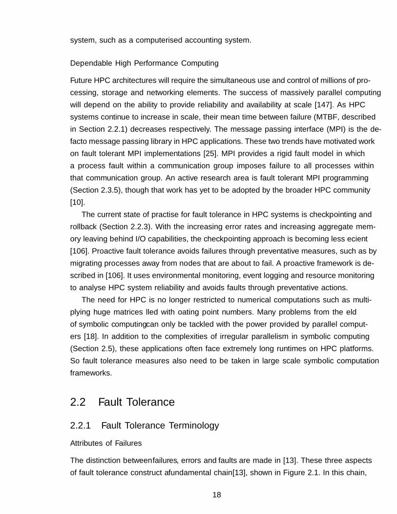
The distinction between failures, errors and faults are made in [13]. These three aspectsof fault tolerance construct a fundamental chain [13], shown in Figure 2.1. In this chain,

18

a failure is an event that occurs when the system does not deliver a service as expectedby its users. A fault is a characteristic of software that can lead to a system error. Anerror can lead to an erroneous system state giving a system behaviour that is unexpectedby system users.

Figure 2.1: Fundamental Chain

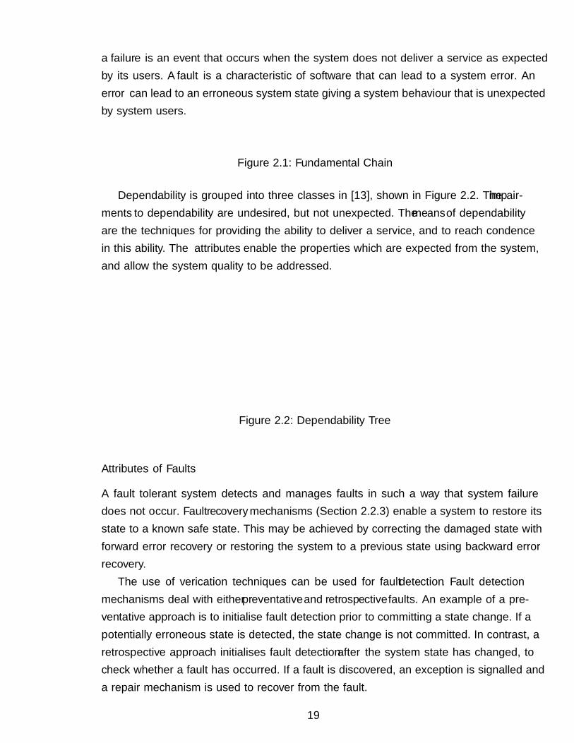
Dependability is grouped into three classes in [13], shown in Figure 2.2. The impair-ments to dependability are undesired, but not unexpected. The means of dependabilityare the techniques for providing the ability to deliver a service, and to reach confidencein this ability. The attributes enable the properties which are expected from the system,and allow the system quality to be addressed.

Figure 2.2: Dependability Tree

Attributes of Faults

A fault tolerant system detects and manages faults in such a way that system failuredoes not occur. Fault recovery mechanisms (Section 2.2.3) enable a system to restore itsstate to a known safe state. This may be achieved by correcting the damaged state withforward error recovery or restoring the system to a previous state using backward errorrecovery.

The use of verification techniques can be used for fault detection. Fault detectionmechanisms deal with either preventative and retrospective faults. An example of a pre-ventative approach is to initialise fault detection prior to committing a state change. If apotentially erroneous state is detected, the state change is not committed. In contrast, aretrospective approach initialises fault detection after the system state has changed, tocheck whether a fault has occurred. If a fault is discovered, an exception is signalled anda repair mechanism is used to recover from the fault.

19

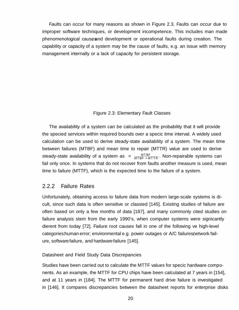
Faults can occur for many reasons as shown in Figure 2.3. Faults can occur due toimproper software techniques, or development incompetence. This includes man madephenomenological causes, and development or operational faults during creation. Thecapability or capacity of a system may be the cause of faults, e.g. an issue with memorymanagement internally or a lack of capacity for persistent storage.

Figure 2.3: Elementary Fault Classes

The availability of a system can be calculated as the probability that it will providethe specified services within required bounds over a specific time interval. A widely usedcalculation can be used to derive steady-state availability of a system. The mean timebetween failures (MTBF) and mean time to repair (MTTR) value are used to derivesteady-state availability of a system as α = MT BF

MT BF +MT T R. Non-repairable systems can

fail only once. In systems that do not recover from faults another measure is used, meantime to failure (MTTF), which is the expected time to the failure of a system.

2.2.2 Failure Rates

Unfortunately, obtaining access to failure data from modern large-scale systems is diffi-cult, since such data is often sensitive or classified [145]. Existing studies of failure areoften based on only a few months of data [187], and many commonly cited studies onfailure analysis stem from the early 1990’s, when computer systems were significantlydifferent from today [72]. Failure root causes fall in one of the following five high-levelcategories: human error; environmental e.g. power outages or A/C failures; network fail-ure, software failure, and hardware failure [145].

Datasheet and Field Study Data Discrepancies

Studies have been carried out to calculate the MTTF values for specific hardware compo-nents. As an example, the MTTF for CPU chips have been calculated at 7 years in [154],and at 11 years in [184]. The MTTF for permanent hard drive failure is investigatedin [146]. It compares discrepancies between the datasheet reports for enterprise disks

20

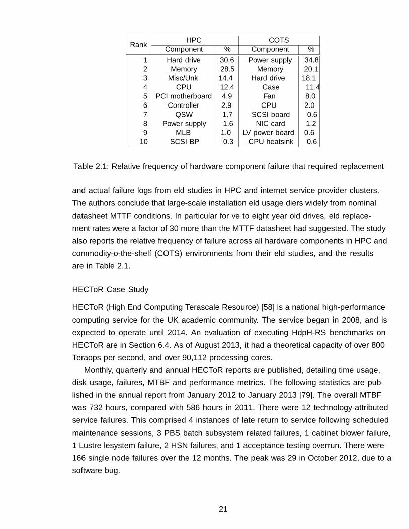
Rank HPC COTSComponent % Component %

1 Hard drive 30.6 Power supply 34.82 Memory 28.5 Memory 20.13 Misc/Unk 14.4 Hard drive 18.14 CPU 12.4 Case 11.45 PCI motherboard 4.9 Fan 8.06 Controller 2.9 CPU 2.07 QSW 1.7 SCSI board 0.68 Power supply 1.6 NIC card 1.29 MLB 1.0 LV power board 0.610 SCSI BP 0.3 CPU heatsink 0.6

Table 2.1: Relative frequency of hardware component failure that required replacement

and actual failure logs from field studies in HPC and internet service provider clusters.The authors conclude that large-scale installation field usage differs widely from nominaldatasheet MTTF conditions. In particular for five to eight year old drives, field replace-ment rates were a factor of 30 more than the MTTF datasheet had suggested. The studyalso reports the relative frequency of failure across all hardware components in HPC andcommodity-off-the-shelf (COTS) environments from their field studies, and the resultsare in Table 2.1.

HECToR Case Study

HECToR (High End Computing Terascale Resource) [58] is a national high-performancecomputing service for the UK academic community. The service began in 2008, and isexpected to operate until 2014. An evaluation of executing HdpH-RS benchmarks onHECToR are in Section 6.4. As of August 2013, it had a theoretical capacity of over 800Teraflops per second, and over 90,112 processing cores.

Monthly, quarterly and annual HECToR reports are published, detailing time usage,disk usage, failures, MTBF and performance metrics. The following statistics are pub-lished in the annual report from January 2012 to January 2013 [79]. The overall MTBFwas 732 hours, compared with 586 hours in 2011. There were 12 technology-attributedservice failures. This comprised 4 instances of late return to service following scheduledmaintenance sessions, 3 PBS batch subsystem related failures, 1 cabinet blower failure,1 Lustre filesystem failure, 2 HSN failures, and 1 acceptance testing overrun. There were166 single node failures over the 12 months. The peak was 29 in October 2012, due to asoftware bug.

21

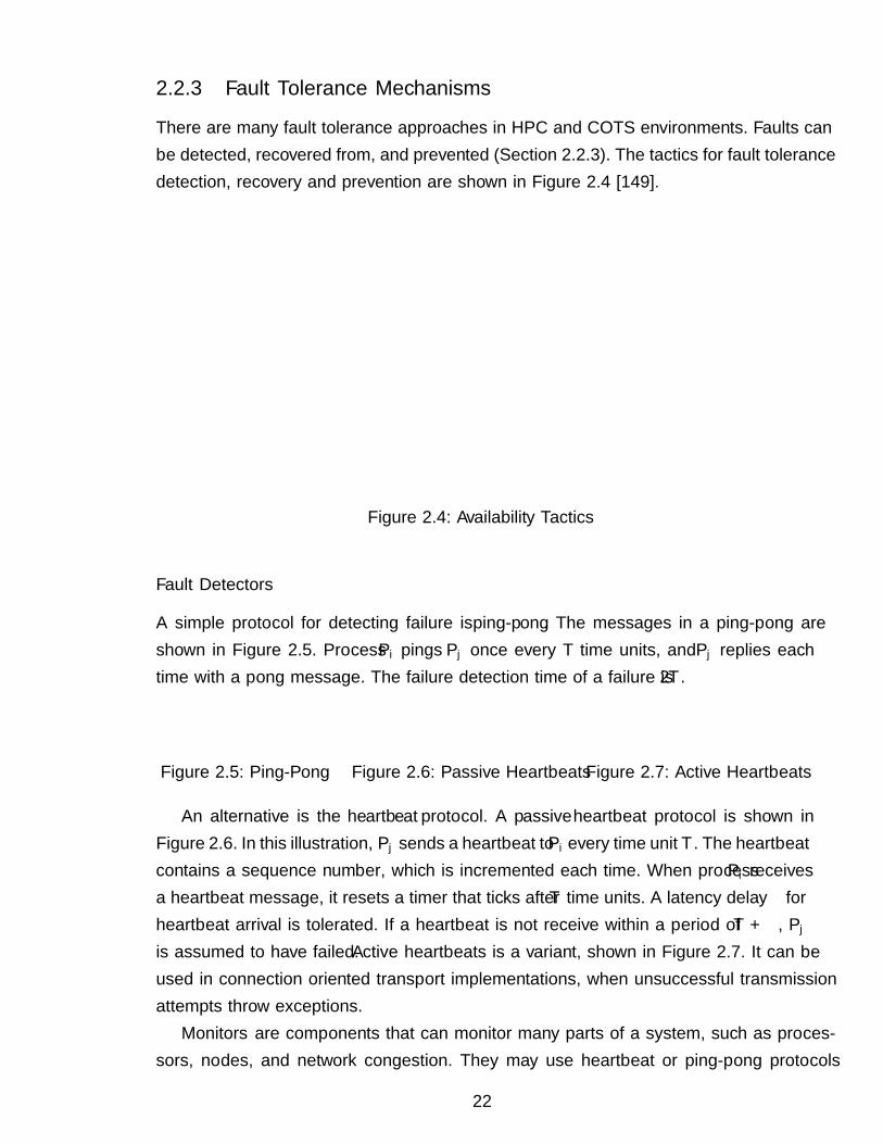
2.2.3 Fault Tolerance Mechanisms

There are many fault tolerance approaches in HPC and COTS environments. Faults canbe detected, recovered from, and prevented (Section 2.2.3). The tactics for fault tolerancedetection, recovery and prevention are shown in Figure 2.4 [149].

Stateresychronisation

Non−stopforwarding

Softwareupgrade

Exceptionhandling

Activeredundancy

Preparationand repair

Passiveredundancy

Fault Recovery

Reintroduction

Shadow

Rollback

Checkpointing

Fault Detection

Exception prevention

Process monitor

Transactions

Fault Prevention

Availability Tactics

Voting

System monitor

Ping

Exception detection

Removal from service

Spare

Heartbeat

Figure 2.4: Availability Tactics

Fault Detectors

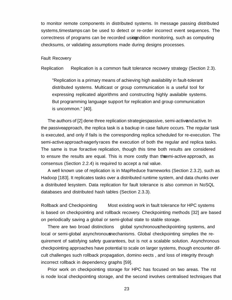
A simple protocol for detecting failure is ping-pong. The messages in a ping-pong areshown in Figure 2.5. Process Pi pings Pj once every T time units, and Pj replies eachtime with a pong message. The failure detection time of a failure is 2T .

Figure 2.5: Ping-Pong Figure 2.6: Passive Heartbeats Figure 2.7: Active Heartbeats

An alternative is the heartbeat protocol. A passive heartbeat protocol is shown inFigure 2.6. In this illustration, Pj sends a heartbeat to Pi every time unit T . The heartbeatcontains a sequence number, which is incremented each time. When process Pi receivesa heartbeat message, it resets a timer that ticks after T time units. A latency delay α forheartbeat arrival is tolerated. If a heartbeat is not receive within a period of T + α, Pj

is assumed to have failed. Active heartbeats is a variant, shown in Figure 2.7. It can beused in connection oriented transport implementations, when unsuccessful transmissionattempts throw exceptions.

Monitors are components that can monitor many parts of a system, such as proces-sors, nodes, and network congestion. They may use heartbeat or ping-pong protocols

22

to monitor remote components in distributed systems. In message passing distributedsystems, timestamps can be used to detect or re-order incorrect event sequences. Thecorrectness of programs can be recorded using condition monitoring, such as computingchecksums, or validating assumptions made during designs processes.

Fault Recovery

Replication Replication is a common fault tolerance recovery strategy (Section 2.3).

"Replication is a primary means of achieving high availability in fault-tolerantdistributed systems. Multicast or group communication is a useful tool forexpressing replicated algorithms and constructing highly available systems.But programming language support for replication and group communicationis uncommon." [40].

The authors of [2] define three replication strategies: passive, semi-active and active. Inthe passive approach, the replica task is a backup in case failure occurs. The regular taskis executed, and only if fails is the corresponding replica scheduled for re-execution. Thesemi-active approach eagerly races the execution of both the regular and replica tasks.The same is true for active replication, though this time both results are consideredto ensure the results are equal. This is more costly than the semi-active approach, asconsensus (Section 2.2.4) is required to accept a final value.

A well known use of replication is in MapReduce frameworks (Section 2.3.2), such asHadoop [183]. It replicates tasks over a distributed runtime system, and data chunks overa distributed filesystem. Data replication for fault tolerance is also common in NoSQLdatabases and distributed hash tables (Section 2.3.3).

Rollback and Checkpointing Most existing work in fault tolerance for HPC systemsis based on checkpointing and rollback recovery. Checkpointing methods [32] are basedon periodically saving a global or semi-global state to stable storage.

There are two broad distinctions — global synchronous checkpointing systems, andlocal or semi-global asynchronous mechanisms. Global checkpointing simplifies the re-quirement of satisfying safety guarantees, but is not a scalable solution. Asynchronouscheckpointing approaches have potential to scale on larger systems, though encounter dif-ficult challenges such rollback propagation, domino effects , and loss of integrity throughincorrect rollback in dependency graphs [59].

Prior work on checkpointing storage for HPC has focused on two areas. The firstis node local checkpointing storage, and the second involves centralised techniques that

23

focus on high-performance parallel systems [125]. The bandwidth between I/O nodes indistributed systems is often regarded as the bottleneck in distributed checkpointing.

Rollback recovery [59] is used when system availability requirements can tolerate theoutage of computing systems during recovery. It offers a resource efficient way of toler-ating failure, compared to other techniques such as replication or transaction processing[60]. In message passing distributed systems, messages induce interprocess dependenciesduring failure-free operation. Upon process failure, these dependencies may force someof the processes that did not fail to roll back to a rollback line, which is called rollbackpropagation [59]. Once a good state is reached, process execution resumes.

Log based rollback-recovery [166] combines checkpointing and logging to enable pro-cesses to replay their execution after a failure beyond the most recent checkpoint. Log-based recovery generally is not susceptible to the domino effect, thereby allowing theprocesses to use uncoordinated checkpointing if desired. Three main techniques of log-ging are optimistic logging, causal logging, and pessimistic logging. Optimistic loggingassumes that messages are logged, but part of these logs can be lost when a fault oc-curs. Systems that implement this approach use either a global coherent checkpoint torollback the entire application, or they assume a small number of fault at one time inthe system. Causal logging is an optimistic approach, checking and building an eventdependency graph to ensure that potential incoherence in the checkpoint will not ap-pear. All processes record their "happened before" activities in an antecedence graph, inaddition to the logging of sent messages. Antecedence graphs are asynchronously sent toa stable storage with checkpoints and message logs. When failures occur, all processes arerolled back to their last checkpoints, using antecedence graphs and message logs. Lastly,pessimistic logging is a transaction log ensuring that no incoherent state can be reachedstarting from a local checkpoint of processes, even with an unbounded number of faults.

Other Mechanisms Degrading operations [12] is a tactic that suspends non-criticalcomponents in order to keep alive the critical aspects of system functionality. Degradationcan reduce or eliminate fault occurrence by gracefully reducing system functionality,rather than causing a complete system failure. Shadowing [17] is used when a previouslyfailed component attempts to rejoin a system. This component will operate in a shadowmode for a period of time, during which its behaviour will be monitored for correctnessand will repopulate its state incrementally as confidence of its reliability increases.

Retry tactics [75] can be an effective way to recover from transient failures — simplyretrying a failed operation may lead to success. Retry strategies have been added to net-working protocols in Section 2.3.4, and also to language libraries such as the gen_server

24

abstraction for Erlang in Section 2.3.6.

Fault Prevention

The prevention of faults is a tactic to avoid or minimise fault occurrence. The componentremoval tactic [68] involves the precautionary removal of a component, before failure isdetected on it. This may involve resetting a node or a network switch, in order to scrublatent faults such as memory leaks, before the accumulation of faults amounts to failure.This tactic is sometimes referred to as software rejuvenation [86].

Predictive modeling [103] is often used with monitors (Section 2.2.3) to gauge thehealth of components or to ensure that the system is operating within its nominal op-erating parameters such as the load on processors or memory, message queue size, andlatency of ping-ack responses (Section 2.2.3). As an example, most motherboards containtemperature sensors, which can be accessed via interfaces like ACPI [41], for monitoringnominal operating parameters. Predictive modeling has been used in a fault tolerant MPI[31], which proactively migrates execution from nodes when it is experiencing intermittentfailure.

2.2.4 Software Based Fault Tolerance

Distributed Algorithms for Reliable Computing

Algorithmic level fault tolerance is a high level fault tolerance approach. Classic examplesinclude leader election algorithms, consensus through voting and quorums, and smoothingresults with probabilistic accuracy bounds.

Leader election algorithms are used to overcome the problem of crashes and linkfailures in both synchronous and asynchronous distributed systems [66]. They can beused in systems that must overcome master node failure in master/slave architectures. Ifa previously elected leader fails, a new election procedure can unilaterally identify a newleader.

Consensus is the agreement of a system status by the fault-free segment of a processpopulation in spite of the possible inadvertent or even malicious spread of disinformationby the faulty segment of that population [14]. Processes propose values, and they alleventually agree on one among these values. This problem is at the core of protocolsthat handle synchronisation, atomic commits, total order broadcasting, and replicatedfile systems.

Using quorums [115] is one way to enhance the availability and efficiency of replicateddata structures. Each quorum can operate on behalf of the system to increase its avail-

25

ability and performance, while an intersection property guarantees that operations doneon distinct quorum preserve consistency [115].

Probabilistic accuracy bounds are used to specify approximation limits on smooth-ing results when some tasks have been lost due to partial failure. A technique presentedin [137] enables computations to survive errors and faults while providing a bound onany resulting output distortion. The fault tolerant approach here is simple: tasks thatencounter faults are discarded. By providing probabilistic accuracy bounds on the dis-tortion of the output, the model allows users to confidently accept results in the presenceof failure, provided the distortion falls with acceptable bounds.

A non-masking approach to fault tolerance is Algorithm Based Fault Tolerance(ABFT) [85]. The approach consists of computing on data that is encoded with somelevel of redundancy. If the encoded results drawn from successful computation has enoughredundancy, it remains possible to reconstruct the missing parts of the results. The ap-plication of this technique is mainly based on the use of parity checksum codes, and iswidely used in HPC platforms [139].

"A system is self-stabilising when, regardless of its initial state, it is guaranteedto arrive at a legitimate state in a finite number of steps." – Edsger W. Dijkstra[53]

Self stabilisation [144] provides a non-masking approach to fault tolerance. A selfstabilising algorithm converges to some predefined set of legitimate states regardless ofits initial state. Due to this property, self-stabilising algorithms provide means for tol-erating transient faults [69]. Self-stabilising algorithms such as [53] use forward recoverystrategies. That is, instead of being externally stopped and rolled-back to a previouscorrect state, the algorithm continues its execution despite the presence of faults, untilthe algorithm corrects itself without external influence.

Fault Tolerant Programming Libraries

In the 1980’s, programmers often had few alternatives faced with choosing a programminglanguage for writing fault tolerant distributed software [5]. At one end of the spectrumwere relatively low-level choices such as C, coupled with a fault tolerance library suchas ISIS [16]. The ISIS system transforms abstract type specifications into fault tolerancedistributed implementations, while insulating users from the mechanisms used to achievefault tolerance. The system itself is based on a small set of communication primitives.Whilst such applications may have enjoyed efficient runtime speeds, the approach forcedthe programmer to deal with the complexities of distributed execution and fault tolerancein a language that is fundamentally sequential.

26

At the other end of the spectrum were high-level languages specifically intended forconstructing fault tolerant application using a given technique, such as Argus [105]. Theselanguages simplified the problems of faults considerably, yet could be overly constrainingif the programmer wanted to use fault tolerance techniques other than the one supportedby the language.

Another approach is to add language extensions to support fault tolerance. An exam-ple is FT-SR [141], an augmentation of the general high-level distributed programminglanguage SR [5], augmented with fault tolerance mechanisms. These include replication,recovery and failure notification. FT-SR was implemented using the x-kernel [87], anOperating System designed for experimenting with communication protocols.

2.3 Classifications of Fault Tolerance Implementa-tions

This section describes examples of fault tolerant distributed software systems. This be-gins with a case study of a reliability extension to a symbolic computation middlewarein Section 2.3.1. The fault tolerance of the MapReduce programming model is describedin Section 2.3.2. A discussion on fault tolerant networking protocols is in Section 2.3.4.As MPI is prominently the current defacto standard for message passing in High Perfor-mance Computing, Section 2.3.5 details numerous fault tolerant MPI implementations.Supervision and fault recovery tactics in HdpH-RS are influenced by Erlang, describedin Sections 2.3.6 and 2.3.7.

2.3.1 Fault Tolerance for DOTS Middleware

A reliability extension to the Distributed Object-Oriented Threads System (DOTS) sym-bolic computation framework [19] is presented in [18]. DOTS was originally intended forthe parallelisation of application belonging to the field of symbolic computation, but ithas also been successfully used in other application domains such as computer graphsand computational number theory.

Programming Model

DOTS provides object-oriented asynchronous remote procedure calls services accessiblefrom C++ through a fork/join programming API, which also supports thread cancella-tion. Additionally, it supports object-serialisation for parameter passing. The program-ming model provides a uniform and high-level programming paradigm over hierarchical

27

multiprocessor systems. Low level details such as message passing and shared memorythreads within a single parallel application are masked from the programmer [18].

Fault Tolerance

The fault tolerance in the reliable extension to DOTS is achieved through asynchronouscheckpointing, realised by two orthogonal approaches. The first is implicit checkpointing.It is completely hidden from the programmer, and no application code modifications arenecessary. The second is explicit checkpointing by adding three new API calls, allowingthe programmer to explicitly control the granularity needs of the application.

To realise the implicit checkpointing approach, function memoization [142] is used.A checkpoint consists of a pair containing the argument and the computed result of athread — whenever a thread has successfully finished its execution, a checkpoint is taken.The checkpointed data is stored in a history table. In the case of a restart of a thread,a replay of communication and computation takes place. If the argument of the threadis present in the history table, the result is taken from the table and immediately sentback to the caller. This strategy is feasible whenever the forked function is stateless.

2.3.2 MapReduce

MapReduce is a programming model and an associated implementation for processingand generating large data sets [49]. Programs written in the functional style are auto-matically parallelisable and can be run on large clusters. Its fault tolerance model makeimplementations such as Hadoop [183] a popular choice for running on COTS archi-tectures, where failure is more common than on HPC architectures. The use of taskre-execution (Section 2.2.3) is the fault tolerance mechanism. Programmers can adoptthe MapReduce model directly, or can use higher level data query languages [163].

The MapReduce architecture involves one master node, and all other nodes are slavenodes. They are responsible both for executing tasks, and hosting chunks of the MapRe-duce distributed filesystem. Fault tolerance is achieved by replicating tasks and dis-tributed filesystem chunks, providing both task parallel and data parallel redundancy. Acomparison between Hadoop and HdpH-RS is made in Section 5.6.2.

2.3.3 Distributed Datastores

Distributed data structures such as distributed hash tables [28] and NoSQL databases[165] often provide flexible performance and fault tolerance parameters. Optimising oneparameter tends to put pressures on others. Brewer’s CAP theorem [26] states a trade

28

off between consistency, availability and partition tolerance — a user can only have twoout of three. An important property of a DHT is a degree of their fault tolerance, whichis the fraction of nodes that can fail without eliminating data or preventing successfulrouting [96].

NoSQL databases do not require fixed table schemas, and are designed to scale hor-izontally and manage huge amounts of data. One of the first NoSQL databases wasGoogle’s proprietary BigTable [33], and subsequent open source NoSQL databases haveemerged including Riak [170]. Riak is a scalable, highly-available, distributed key/valuestore built using Erlang/OTP (Section 2.3.7). It is resilient to failure through a quorumbased eventual consistency model, based on Amazon’s Dynamo paper [50].

2.3.4 Fault Tolerant Networking Protocols

There are many APIs for connecting and exchanging data between network peers. In 1981,the Internet Protocol (IP) [132] began the era of ubiquitous networking. When processeson two different computer communicate, the most often do so using the TCP protocol[156]. It offers a convenient bi-directional bytestream interface for communication. It alsohides most communication problems from the programmer, such as message losses andmessage duplicates, overcome using sequence numbers and acknowledgements.

TCP/IP uses the sockets interfaces supported by many Operating Systems. It is thewidely used protocol that Internet services rely upon. It has a simple API that providesstream and datagram modes, and is robust to failure. It does not provide the collectivecommunications or one-sided operations that MPI provides.

FT-TCP [3] is an architecture that allows a replicated service to survive crasheswithout breaking its TCP connections. It is a failover software implementation thatwraps the TCP stack to intercept all communication, and is based on message logging.

In the HPC domain, MPI is the dominant interface for inter-process communication[10]. Designed for maximum scalability, MPI has a richer though also more complex APIthan sockets. The complications of fault tolerant MPI are detailed in Section 2.3.5.

There are numerous highly specialised vendor APIs for distributed network peer com-munication. Popular examples include Cray Portals [27], IBM’s LAPI [150] and InfinibandVerbs [8]. Verbs has support for two-sided and one-sided asynchronous operations, andbuffer management is left to the application. Infiniband [107] is a switched fabric commu-nications link commonly used in HPC clusters. It features high throughput, low latencyand is designed for scalability.

The performance of each interface varies wildly in terms of speed, portability, robust-ness and complexity. The design of each balance the trade-off between these performance

29

Sockets MPI Specialised APIsPerformance No Yes YesScalability No Yes VariesPortability Yes Yes NoRobustness Yes No VariesSimplicity Yes No Varies

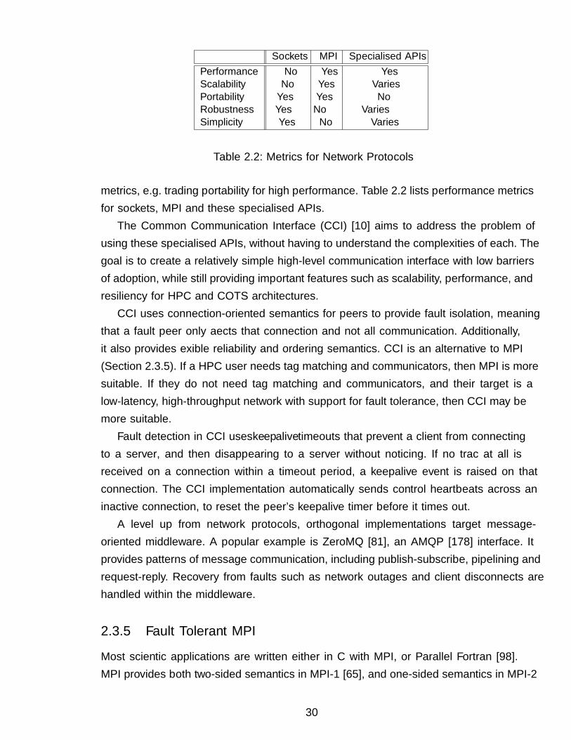
Table 2.2: Metrics for Network Protocols

metrics, e.g. trading portability for high performance. Table 2.2 lists performance metricsfor sockets, MPI and these specialised APIs.

The Common Communication Interface (CCI) [10] aims to address the problem ofusing these specialised APIs, without having to understand the complexities of each. Thegoal is to create a relatively simple high-level communication interface with low barriersof adoption, while still providing important features such as scalability, performance, andresiliency for HPC and COTS architectures.

CCI uses connection-oriented semantics for peers to provide fault isolation, meaningthat a fault peer only affects that connection and not all communication. Additionally,it also provides flexible reliability and ordering semantics. CCI is an alternative to MPI(Section 2.3.5). If a HPC user needs tag matching and communicators, then MPI is moresuitable. If they do not need tag matching and communicators, and their target is alow-latency, high-throughput network with support for fault tolerance, then CCI may bemore suitable.

Fault detection in CCI uses keepalive timeouts that prevent a client from connectingto a server, and then disappearing to a server without noticing. If no traffic at all isreceived on a connection within a timeout period, a keepalive event is raised on thatconnection. The CCI implementation automatically sends control heartbeats across aninactive connection, to reset the peer’s keepalive timer before it times out.

A level up from network protocols, orthogonal implementations target message-oriented middleware. A popular example is ZeroMQ [81], an AMQP [178] interface. Itprovides patterns of message communication, including publish-subscribe, pipelining andrequest-reply. Recovery from faults such as network outages and client disconnects arehandled within the middleware.

2.3.5 Fault Tolerant MPI

Most scientific applications are written either in C with MPI, or Parallel Fortran [98].MPI provides both two-sided semantics in MPI-1 [65], and one-sided semantics in MPI-2

30

[123]. It also provides tag matching and collective operations.Paradoxically however, fault tolerant MPI programming for users is challenging, and

they are often forced to handle faults programmatically. This will become increasinglyproblematic as MPI is scaled to massively parallel exascale systems as soon as 2015 [62].The original MPI standards specify very limited features related to reliability and faulttolerance [73]. Based on the early standards, an entire application is shut down when oneof the executing processors experiences a failure, as fault handling is per communicatorgroup, and not be peer. The default behaviour in MPI is that any fault will typicallybring down the entire communicator.

This section describes several approaches to achieve fault tolerance in MPI programsincluding the use of checkpointing, modifying the semantics of existing MPI functions toprovide more fault-tolerant behaviour, or defining extensions to the MPI specification.

Fault Tolerant MPI Implementations

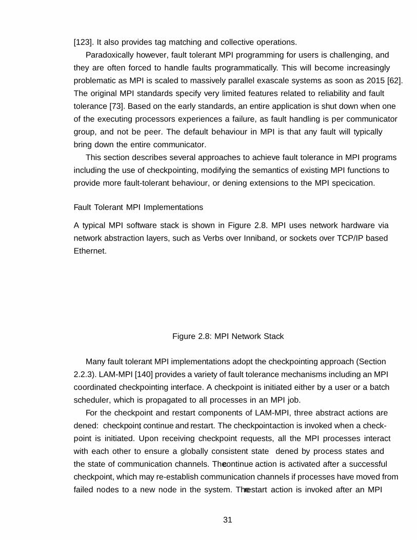
A typical MPI software stack is shown in Figure 2.8. MPI uses network hardware vianetwork abstraction layers, such as Verbs over Infiniband, or sockets over TCP/IP basedEthernet.

IPoIB

Ethernet

IP

TCP

Sockets API

Cray GNI

Gemini Infiniband

Verbs

Application

MPI

Figure 2.8: MPI Network Stack

Many fault tolerant MPI implementations adopt the checkpointing approach (Section2.2.3). LAM-MPI [140] provides a variety of fault tolerance mechanisms including an MPIcoordinated checkpointing interface. A checkpoint is initiated either by a user or a batchscheduler, which is propagated to all processes in an MPI job.

For the checkpoint and restart components of LAM-MPI, three abstract actions aredefined: checkpoint, continue and restart. The checkpoint action is invoked when a check-point is initiated. Upon receiving checkpoint requests, all the MPI processes interactwith each other to ensure a globally consistent state — defined by process states andthe state of communication channels. The continue action is activated after a successfulcheckpoint, which may re-establish communication channels if processes have moved fromfailed nodes to a new node in the system. The restart action is invoked after an MPI

31

process has been restored from a prior checkpoint. This action will almost always needto re-discover its MPI process peers and re-establish communication channels to them.

The MPICH-V [24] environment encompasses a communication library based onMPICH [74], and a runtime environment. MPICH-V provides an automatic volatilitytolerant MPI environment based on uncoordinated checkpointing and rollback and dis-tributed message logging. Unlike other checkpointing systems such as LAM-MPI, thecheckpointing in MPICH-V is asynchronous, avoiding the risk that some nodes may un-available during a checkpointing routine.

Cocheck [155] is an independent application making an MPI parallel application faulttolerant. Cocheck sits at the runtime level on top of a message passing library, providinga consistency at a level above the message passing system. Cocheck coordinates theapplication processes checkpoints and flushes the communication channels of the targetapplications using a Chandy-Lamport’s algorithm [52]. The program itself is not aware ofcheckpointing or rollback routines. The checkpoint and rollback procedures are managedby a centralised coordinator.

FT-MPI [51] takes an alternative approach, by modifying the MPI semantics in orderto recover from faults. Upon detecting communication failures, FT-MPI marks the asso-ciated node as having a possible error. All other nodes involved with that communicatorare informed. It extends the MPI communicator states, and default MPI process sates[63].

LA-MPI [11] has numerous fault tolerance features including application checksum-ming, message re-transmission and automatic message re-routing. The primary motiva-tion for LA-MPI is fault tolerance at the data-link and transport levels. It reliably deliversmessages in the presence of I/O bus, network card and wire-transmission errors, and soguarantees delivery of in-flight message after such failures.

2.3.6 Erlang

Erlang is a distributed functional programming language and is becoming a popularsolution for developing highly concurrent, distributed soft real-time systems. The Erlangapproach to failures is let it crash and another process will correct the error [7].

New processes are created with a spawn primitive. The return value of a spawn call isa process ID (PID). One process can monitor another by calling monitor on its PID. Whena process dies, A DOWN message is sent to all monitoring processes. For convenience, thefunction spawn_monitor atomically spawns a new process and monitors it. An example ofusing spawn_monitor is shown in Listing 2.1. The time_bomb/1 function ticks down fromN every second. When N reaches 0, the process dies. The repeat_explosion/2 function

32

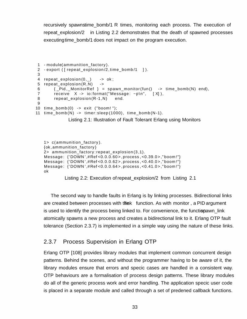
recursively spawns time_bomb/1 R times, monitoring each process. The execution ofrepeat_explosion/2 in Listing 2.2 demonstrates that the death of spawned processesexecuting time_bomb/1 does not impact on the program execution.

1 -module(ammunition_factory).2 -export([repeat_explosion /2, time_bomb /1]).34 repeat_explosion (0,_) -> ok;5 repeat_explosion(R,N) ->6 {_Pid ,_MonitorRef} = spawn_monitor(fun() -> time_bomb(N) end),7 receive X -> io:format("Message: ~p\n",[X]),8 repeat_explosion(R-1,N) end.910 time_bomb (0) -> exit("boom!");11 time_bomb(N) -> timer:sleep (1000) , time_bomb(N-1).

Listing 2.1: Illustration of Fault Tolerant Erlang using Monitors

1> c(ammunition_factory ).{ok,ammunition_factory}2> ammunition_factory:repeat_explosion (3 ,1).Message: {’DOWN ’,#Ref <0.0.0.60 > , process ,<0.39.0>," boom !"}Message: {’DOWN ’,#Ref <0.0.0.62 > , process ,<0.40.0>," boom !"}Message: {’DOWN ’,#Ref <0.0.0.64 > , process ,<0.41.0>," boom !"}ok

Listing 2.2: Execution of repeat_explosion/2 from Listing 2.1

The second way to handle faults in Erlang is by linking processes. Bidirectional linksare created between processes with the link function. As with monitor, a PID argumentis used to identify the process being linked to. For convenience, the function spawn_link

atomically spawns a new process and creates a bidirectional link to it. Erlang OTP faulttolerance (Section 2.3.7) is implemented in a simple way using the nature of these links.

2.3.7 Process Supervision in Erlang OTP

Erlang OTP [108] provides library modules that implement common concurrent designpatterns. Behind the scenes, and without the programmer having to be aware of it, thelibrary modules ensure that errors and specific cases are handled in a consistent way.OTP behaviours are a formalisation of process design patterns. These library modulesdo all of the generic process work and error handling. The application specific user codeis placed in a separate module and called through a set of predefined callback functions.

33

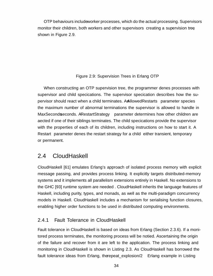
OTP behaviours include worker processes, which do the actual processing. Supervisorsmonitor their children, both workers and other supervisors — creating a supervision tree,shown in Figure 2.9.

Figure 2.9: Supervision Trees in Erlang OTP

When constructing an OTP supervision tree, the programmer defines processes withsupervisor and child specifications. The supervisor specification describes how the su-pervisor should react when a child terminates. An AllowedRestarts parameter specifiesthe maximum number of abnormal terminations the supervisor is allowed to handle inMaxSeconds seconds. A RestartStrategy parameter determines how other children areaffected if one of their siblings terminates. The child specifications provide the supervisorwith the properties of each of its children, including instructions on how to start it. ARestart parameter defines the restart strategy for a child — either transient, temporaryor permanent.

2.4 CloudHaskell

CloudHaskell [61] emulates Erlang’s approach of isolated process memory with explicitmessage passing, and provides process linking. It explicitly targets distributed-memorysystems and it implements all parallelism extensions entirely in Haskell. No extensions tothe GHC [93] runtime system are needed . CloudHaskell inherits the language features ofHaskell, including purity, types, and monads, as well as the multi-paradigm concurrencymodels in Haskell. CloudHaskell includes a mechanism for serialising function closures,enabling higher order functions to be used in distributed computing environments.

2.4.1 Fault Tolerance in CloudHaskell

Fault tolerance in CloudHaskell is based on ideas from Erlang (Section 2.3.6). If a moni-tored process terminates, the monitoring process will be notified. Ascertaining the originof the failure and recover from it are left to the application. The process linking andmonitoring in CloudHaskell is shown in Listing 2.3. As CloudHaskell has borrowed thefault tolerance ideas from Erlang, the repeat_explosion/2 Erlang example in Listing

34

2.1 could similarly be constructed with CloudHaskell using spawnMonitor in 2.3. At ahigher level, another fault tolerance abstraction is redundant distributed data structures.The author has contributed [160] to the development of a fault tolerant Chord-baseddistributed hash table in CloudHaskell.

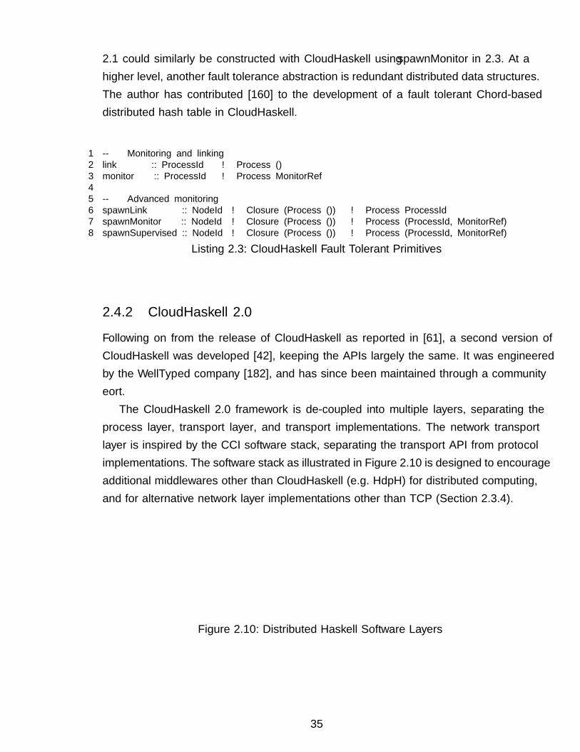
1 -- ∗ Monitoring and linking2 link :: ProcessId → Process ()3 monitor :: ProcessId → Process MonitorRef45 -- ∗ Advanced monitoring6 spawnLink :: NodeId → Closure (Process ()) → Process ProcessId7 spawnMonitor :: NodeId → Closure (Process ()) → Process (ProcessId, MonitorRef)8 spawnSupervised :: NodeId → Closure (Process ()) → Process (ProcessId, MonitorRef)

Listing 2.3: CloudHaskell Fault Tolerant Primitives

2.4.2 CloudHaskell 2.0

Following on from the release of CloudHaskell as reported in [61], a second version ofCloudHaskell was developed [42], keeping the APIs largely the same. It was engineeredby the WellTyped company [182], and has since been maintained through a communityeffort.

The CloudHaskell 2.0 framework is de-coupled into multiple layers, separating theprocess layer, transport layer, and transport implementations. The network transportlayer is inspired by the CCI software stack, separating the transport API from protocolimplementations. The software stack as illustrated in Figure 2.10 is designed to encourageadditional middlewares other than CloudHaskell (e.g. HdpH) for distributed computing,and for alternative network layer implementations other than TCP (Section 2.3.4).

CloudHaskell

TCP UDP MPI

meta−parHdpH Middlewares

Transports

Transport APInetwork−transport

Figure 2.10: Distributed Haskell Software Layers

35

2.5 SymGridParII

Symbolic computation is an important area of both Mathematics and Computer Science,with many large computations that would benefit from parallel execution. Symbolic com-putations are, however, challenging to parallelise as they have complex data and controlstructures, and both dynamic and highly irregular parallelism. In contrast to many ofthe numerical problems that are common in HPC applications, symbolic computationcannot easily be partitioned into many subproblems of similar type and complexity.

The SymGridPar (SGP) framework [104] was developed to address these challengeson small-scale parallel architectures. However, the multicore revolution means that thenumber of cores and the number of failures are growing exponentially, and that thecommunication topology is becoming increasingly complex. Hence an improved parallelsymbolic computation framework is required. SymGridParII is a successor to SGP thatis designed to provide scalability onto 106 cores, and hence also provide fault tolerance.

The main goal in developing SGPII [112] as a successor to SGP is scaling symboliccomputation to architectures with 106 cores. This scale necessitates a number of furtherdesign goals, one of which is fault tolerance, to cope with increasingly frequent componentfailures (Section 2.2.2).

2.6 HdpH

The realisation of SGPII is Haskell Distributed Parallel Haskell (HdpH). The language isa shallowly embedded parallel extension of Haskell that supports high-level implicit andexplicit parallelism.

To handle the complex nature of symbolic applications, HdpH supports dynamic andirregular parallelism. Task placement in SGPII should avoid explicit choice whereverpossible. Instead, choice should be semi-explicit, so the programmer decides which tasksare suitable for parallel execution and possibly at what distance from the current nodethey should be executed. HdpH therefore provides high-level semi-explicit parallelism.The programmer is not required to explicitly place tasks on specific node, instead idlenodes seek work automatically. The HdpH implementation continuously manages load,ensuring that all nodes are utilised effectively.

2.6.1 HdpH Language Design

HdpH supports two parallel programming models. The first is a continuation passingstyle [167], when the language primitives are used directly. This supports a dataflow

36

programming style. The second programming model is through the use of higher orderparallel skeletons. Algorithmic skeletons have been developed on top of the HdpH prim-itives to provide higher order parallel skeletons, inspired by the Algorithms + Skeletons= Parallelism paper [171].

The HdpH language is strongly influenced by two Haskell libraries, that lift function-ality normally provided by a low-level RTS to the Haskell level.

Par Monad [118] A shallowly embedded domain specific language (DSL) for determin-istic shared-memory parallelism. The HdpH primitives extend the Par monad fordistributed memory parallelism.

Closure serialisation in CloudHaskell HdpH extends the closure serialisation tech-niques from CloudHaskell (Section 2.4) to support polymorphic closure transfor-mation, which is used to implement high-level coordination abstractions.

2.6.2 HdpH Primitives

The API in Figure 2.4 expose scheduling primitives for both shared and distributed mem-ory parallelism. The shared memory primitives are inherited from the Par monad. ThePar type constructor is a monad for encapsulating a parallel computation. To commu-nicate the results of computation (and to block waiting for their availability), threadsemploy IVars, which are essentially mutable variables that are writable exactly once. Auser can create an IVar with new, write to them with put, and blocking read from themwith get.

The basic primitive for shared memory scheduling is fork, which forks a new threadand returns nothing. The two primitives for distributed memory parallelism are spark

and pushTo. The former operates much like fork, generating a computation that may beexecuted on another node. The pushTo primitive is similar except that it eagerly pusheda computation to a target node, where it eagerly unwrapped from its closured form andexecuted. In contrast to this scheduling strategy, spark just stores its argument in alocal sparkpool, where it sits waiting to be distributed, or scheduled by an on-demandwork-stealing scheduler, described in Section 2.6.4. Closures are constructed with themkClosure function. It safely converts a quoted thunk i.e. an expression in TemplateHaskell’s quotation brackets [|..|] into a quoted Closure [114].

2.6.3 Programming Example with HdpH

A HdpH implementation of the Fibonacci micro-benchmark is shown in Listing 2.5. Ituses spark to allow the lazy work stealing HdpH scheduling to (maybe) evaluate fib n-1,

37

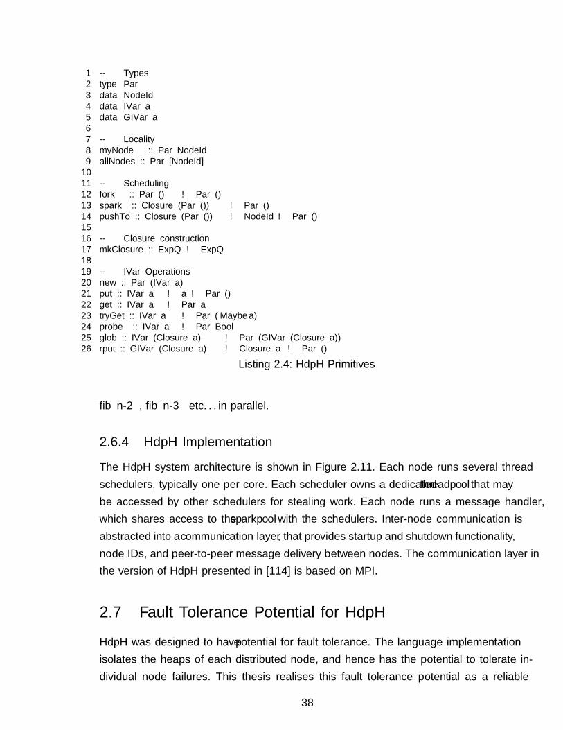
1 -- ∗ Types2 type Par3 data NodeId4 data IVar a5 data GIVar a67 -- ∗ Locality8 myNode :: Par NodeId9 allNodes :: Par [NodeId]1011 -- ∗ Scheduling12 fork :: Par () → Par ()13 spark :: Closure (Par ()) → Par ()14 pushTo :: Closure (Par ()) → NodeId → Par ()1516 -- ∗ Closure construction17 mkClosure :: ExpQ → ExpQ1819 -- ∗ IVar Operations20 new :: Par (IVar a)21 put :: IVar a → a → Par ()22 get :: IVar a → Par a23 tryGet :: IVar a → Par (Maybe a)24 probe :: IVar a → Par Bool25 glob :: IVar (Closure a) → Par (GIVar (Closure a))26 rput :: GIVar (Closure a) → Closure a → Par ()

Listing 2.4: HdpH Primitives

fib n-2, fib n-3 etc. . . in parallel.

2.6.4 HdpH Implementation

The HdpH system architecture is shown in Figure 2.11. Each node runs several threadschedulers, typically one per core. Each scheduler owns a dedicated threadpool that maybe accessed by other schedulers for stealing work. Each node runs a message handler,which shares access to the sparkpool with the schedulers. Inter-node communication isabstracted into a communication layer, that provides startup and shutdown functionality,node IDs, and peer-to-peer message delivery between nodes. The communication layer inthe version of HdpH presented in [114] is based on MPI.

2.7 Fault Tolerance Potential for HdpH

HdpH was designed to have potential for fault tolerance. The language implementationisolates the heaps of each distributed node, and hence has the potential to tolerate in-dividual node failures. This thesis realises this fault tolerance potential as a reliable

38

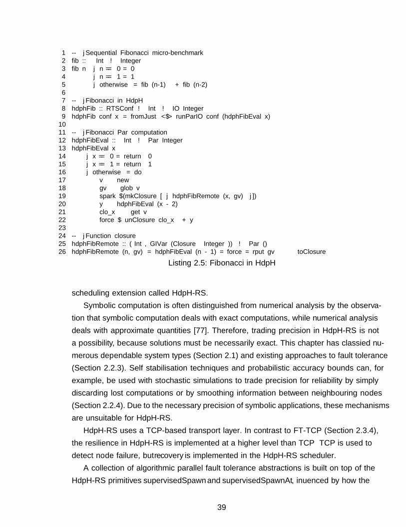
1 -- |Sequential Fibonacci micro-benchmark2 fib :: Int → Integer3 fib n | n == 0 = 04 | n == 1 = 15 | otherwise = fib (n-1) + fib (n-2)67 -- |Fibonacci in HdpH8 hdphFib :: RTSConf → Int → IO Integer9 hdphFib conf x = fromJust <$> runParIO conf (hdphFibEval x)1011 -- |Fibonacci Par computation12 hdphFibEval :: Int → Par Integer13 hdphFibEval x14 | x == 0 = return 015 | x == 1 = return 116 | otherwise = do17 v ← new18 gv ← glob v19 spark $(mkClosure [ | hdphFibRemote (x, gv) |])20 y ← hdphFibEval (x - 2)21 clo_x ← get v22 force $ unClosure clo_x + y2324 -- |Function closure25 hdphFibRemote :: (Int, GIVar (Closure Integer)) → Par ()26 hdphFibRemote (n, gv) = hdphFibEval (n - 1) »= force »= rput gv ◦ toClosure

Listing 2.5: Fibonacci in HdpH

scheduling extension called HdpH-RS.Symbolic computation is often distinguished from numerical analysis by the observa-

tion that symbolic computation deals with exact computations, while numerical analysisdeals with approximate quantities [77]. Therefore, trading precision in HdpH-RS is nota possibility, because solutions must be necessarily exact. This chapter has classified nu-merous dependable system types (Section 2.1) and existing approaches to fault tolerance(Section 2.2.3). Self stabilisation techniques and probabilistic accuracy bounds can, forexample, be used with stochastic simulations to trade precision for reliability by simplydiscarding lost computations or by smoothing information between neighbouring nodes(Section 2.2.4). Due to the necessary precision of symbolic applications, these mechanismsare unsuitable for HdpH-RS.

HdpH-RS uses a TCP-based transport layer. In contrast to FT-TCP (Section 2.3.4),the resilience in HdpH-RS is implemented at a higher level than TCP — TCP is used todetect node failure, but recovery is implemented in the HdpH-RS scheduler.

A collection of algorithmic parallel fault tolerance abstractions is built on top of theHdpH-RS primitives supervisedSpawn and supervisedSpawnAt, influenced by how the

39

spark pool

registry IVars node table

scheduler scheduler

Node 1

IO threads IO threads

Node 2

thread pools

spark pool

node table

msg handler

scheduler

msg handler

registry IVars

thread pools

Haskell heaps

MPI network

Figure 2.11: HdpH System Architecture

supervision behaviour in Erlang OTP (Section 2.3.7) abstracts over the lower level linkprimitive. The distinction between fault tolerance in CloudHaskell (Section 2.4) andHdpH-RS is how failures are handled. Although CloudHaskell provides the necessaryprimitives for fault tolerance i.e. process linking and monitoring (Section 2.4.1), parentprocesses must be programmed to recover from detected failures. In contrast, the HdpH-RS scheduler handles and recovers from faults — the programmer does not need toprogram with faults in mind.

40

Chapter 3

Designing a Fault TolerantProgramming Language forDistributed Memory Scheduling

This chapter presents the design of a reliability extension to HdpH, HdpH-RS. The de-sign of HdpH-RS is sensitive to the complexities of asynchronous distributed systems —tracking task migration, detecting failure, and identifying at-risk tasks in the presenceof failure. The design forms a foundation for the validation and implementation of areliable distributed scheduler for HdpH-RS in Chapters 4 and 5. The design of HdpH-RShas three elements:

1. Fault tolerant programming primitives The HdpH API is extended with thespawn family of primitives for fault tolerant task scheduling, introduced in Section3.3.2.

2. A small-step operational semantics An operational semantics for a simplifieddefinition for the HdpH-RS primitives is given in Section 3.4. It describes the small-step reduction semantics on states for each primitive. Executions through thesesmall-step transitions is in Section 3.4.4.

3. A reliable distributed scheduler The algorithms for reliable scheduling is inSection 3.5.4, and are then illustrated with examples in Section 3.5.5. HdpH-RS isresilient to single node and simultaneous failure (Section 3.5.5), such as networkpartitioning where multiple nodes become detached from the root node at once. Thescheduler detects network connection failures due to failures of nodes, networkinghardware or software crashes. Failures are encapsulated with isolated heaps for eachnode, so the loss of one node does not damage other nodes in the architecture.

41

Why is such a rigorous design processes needed? Would not a carefully constructedreliable scheduler suffice, with human intuition as the verification step in its design?Asynchronous message passing in distributed systems make it extremely difficult maintaina correct understanding of task location, occurrence of task evaluation, and node failure.The work stealing system architecture of HdpH complicates matters further — whentasks are created they can migrate between nodes before they are either evaluated orlost in the presence of failure. Marrying a verified scheduler model and a formalisedoperational semantics as a design process adds confidence that the HdpH-RS schedulerwill evaluate tasks correctly and be resilient to failure.

Operational Semantics

Scheduler

HdpH−RS

Primitives

SPIN Model Partial Abstraction

Abstraction

Figure 3.1: Abstraction of Design, Validation & Implementation of HdpH-RS

The relationship between the HdpH-RS primitives and scheduler design (Section3.3.2), reliable scheduling properties verified with model checking (Chapter 4), the oper-ational semantics (Section 3.4) and Haskell realisation (Chapter 5) are depicted in Figure3.1. The implementation honours the Promela model verified by SPIN, and the small-stepoperational semantics. Therefore, the scheduling algorithms in Section 3.5.4, the Promelamodel in Chapter 4, and implementation in Chapter 5 are frequently cross-referenced toshow a consistency from design, through validation, to implementation.

3.1 Supervised Workpools Prototype

A supervised workpools prototype is a strong influence on the HdpH-RS fault tol-erant programming primitives and reliable scheduling design. The design and imple-mentation has been published [164], and is described in detail in Appendix A.1. Theconcept of exposing the fault tolerant programming primitives supervisedSpawn andsupervisedSpawnAt is influenced by the supervisedWorkpoolEval primitive. All threeallow the user to opt-in to reliable scheduling of tasks. The workpool hides task schedul-ing, failure detection and task replication from the programmer. Moreover, workpools canbe nested to form fault-tolerant hierarchies, which is essential for scaling up to massivelyparallel platforms.

On top of the supervised workpool, two algorithmic skeletons were produced, encapsu-

42

lating parallel-map and divide-and-conquer patterns. The technique of abstracting faulttolerant parallel patterns in this way has been elaborated in HdpH-RS, which exposes10 fault tolerant algorithmic skeletons (Section 6.1.2). The supervised workpool achievedfault tolerance using three techniques — keeping track of where tasks are sent, detectingfailure, and replicating tasks that may be lost because of failure. These techniques areextended in the HdpH-RS implementation.

The main limitation of the supervised workpool prototype is its scheduling capability.Tasks are scheduled eagerly and preemptively. There is no opportunity for load balancingbetween overloaded and idle nodes. The challenge of fault tolerance is greatly increasedwhen a distributed scheduler is required to supervise tasks that can migrate to idlenodes. The HdpH-RS design and implementation is a refined elaboration of the supervisedworkpools prototype. It supports work stealing, spark location tracking, failure detection,and spark and thread replication. The HdpH-RS implementation feature set matches theHdpH language and scheduler, with the exception of fish hopping (Section 3.5.2). Failure-free runtime overheads are comparative to HdpH, even when scaling to 1400 cores (Section6.4.2).

3.2 Introducing Work Stealing Scheduling

To minimise application completion times, load-balancing algorithms try to keep all nodesbusy performing application related work. If work is not equally distributed betweennodes, then some nodes may be idle while others may hold more work than they can im-mediately execute, wasting the potential performance that a parallel environment offers.The efficiency gained with load balancing are set against communication costs. The dis-tribution of tasks causes communication among the nodes in addition to task execution[176]. Minimising both the idle time and communication overhead are conflicting goals,so load-balancing algorithms have to carefully balance communication-related overheadand processor idle time [152].

Parallel symbolic computation is a good example where load balancing is needed.Symbolic computations often exhibit irregular parallelism, which in turn leads to lesscommon patterns of parallel behaviour [77]. These applications pose significant challengesto achieving scalable performance on large-scale multicore clusters, often require ongoingdynamic load balancing in order to maintain efficiency [54].

Load balancing algorithms have been designed for single site clusters e.g. [189] andwide area networks e.g. [177]. There are many design possibilities for load balancing inwide area networks to consider. These include cluster-aware hierarchical stealing and

43

cluster-aware load balanced stealing [176]. For single-site clusters, two common loadbalancing methods are work pushing initiated by an overloaded node, and work stealinginitiated by an idle node.

With random work pushing, a node checks after creating or receiving a task whetherthe task queue length exceeds a certain threshold value. If this is the case, a task fromthe queue’s tail is pushed to a randomly chosen node. This approach aims at minimisingnode idle time because tasks are pushed ahead of time, before they are actually needed.Random work stealing attempts to steal a job from a randomly selected node when a nodefinds its own work queue empty, repeating steal attempts until it succeeds. This approachminimises communication overhead at the expense of idle time. No communication isperformed until a node becomes idle, but then it has to wait for a new task to arrive.When the system load is high, no communication is needed, causing the system to behavewell under high loads [176].

The HdpH-RS language supports both work pushing and work stealing, thanks to theinherited design and implementation of the HdpH scheduler (Section 2.6). The languagesupports implicit task placement with spawn, and explicit placement with spawnAt, de-scribed in Section 3.3.2. Sparkpools hold sparks (closured expressions) that can migratebetween nodes in the HdpH architecture. When a node becomes idle, the scheduler looksfor work. If the local sparkpool is empty, it will fish for work from remote nodes. Ifthe local sparkpool holds a spark, it is unpacked and added to a local threadpool to beevaluated. In this form, threads cannot migrate (again) to other nodes.

This chapter adopts a common terminology for work stealing schedulers [20]. In workstealing strategies, nodes assume dynamically inherited scheduling roles during runtime.Thieves are idle nodes with few tasks to compute, or no tasks at all. They steal fromvictims that host more work than they can immediately execute. A thief will randomlyselect a victim, avoiding deterministic work stealing loops between only a subset of nodes.Fishing is the act of a thief attempting to steal work from a chosen victim. The HdpH-RS terminology is described in Section 3.3.1, for now a spark can be regarded as acomputation that can migrate between nodes. Two examples of the HdpH fishing protocolare shown in Figure 3.2. Thieving node C attempts to steal a spark from victim nodeB with a fish message, and is successful. Thieving node D is unsuccessful in its fishingmessage to victim node B.

44

Node Bvictim

Node Cthief1

Node Dthief2

FISH

SCHEDULE

FISH

NOWORK

Figure 3.2: Two HdpH Work Stealing Scenarios

3.3 Reliable Scheduling for Fault Tolerance

The fault tolerance is realised in HdpH-RS with two new programming primitives, anda resilient scheduler.

Fault tolerance API The HdpH-RS API provides four new primitives. They provideimplicit and explicit parallelism. They are spawn and spawnAt, and two fault tol-erant primitives supervisedSpawn and supervisedSpawnAt. The definition of aspawned computation defines a close pairing between tasks and values, describedin Section 3.3.2.

Reliable scheduler To support the two fault tolerance primitives, the HdpH-RS sched-uler includes 7 additional RTS messages, compared to the HdpH scheduler. Therecovery of supervised tasks is described algorithmically in Section 3.5.4, and theoperational semantics for recovery is given in Section 3.4. The additional runtimesystem (RTS) messages in the reliable scheduler are described in Section 3.5.1.

The language design provides opt-in reliability. The original plan for the HdpH-RSAPI was to use the existing HdpH scheduling API, and adding a scheduler flag to indicatethat fault tolerant work stealing should be used. An operational semantics (Section 3.4)was attempted for the fault tolerant versions of the HdpH task creation primitives sparkand pushTo. The semantics were complicated by a lack of enforced coupling betweentasks and values (IVars). A simpler set of task creation primitives, the spawn family,were designed as a result. The spawn family of primitives (Section 3.3.2) enforce a one-to-one relationship between task expressions and IVars.

3.3.1 HdpH-RS Terminology

Table 3.1 defines a consistent terminology to describe tasks, values, and nodes. Theterminology is tied closely to the spawn family of primitives, introduced in Section 3.3.2.

45

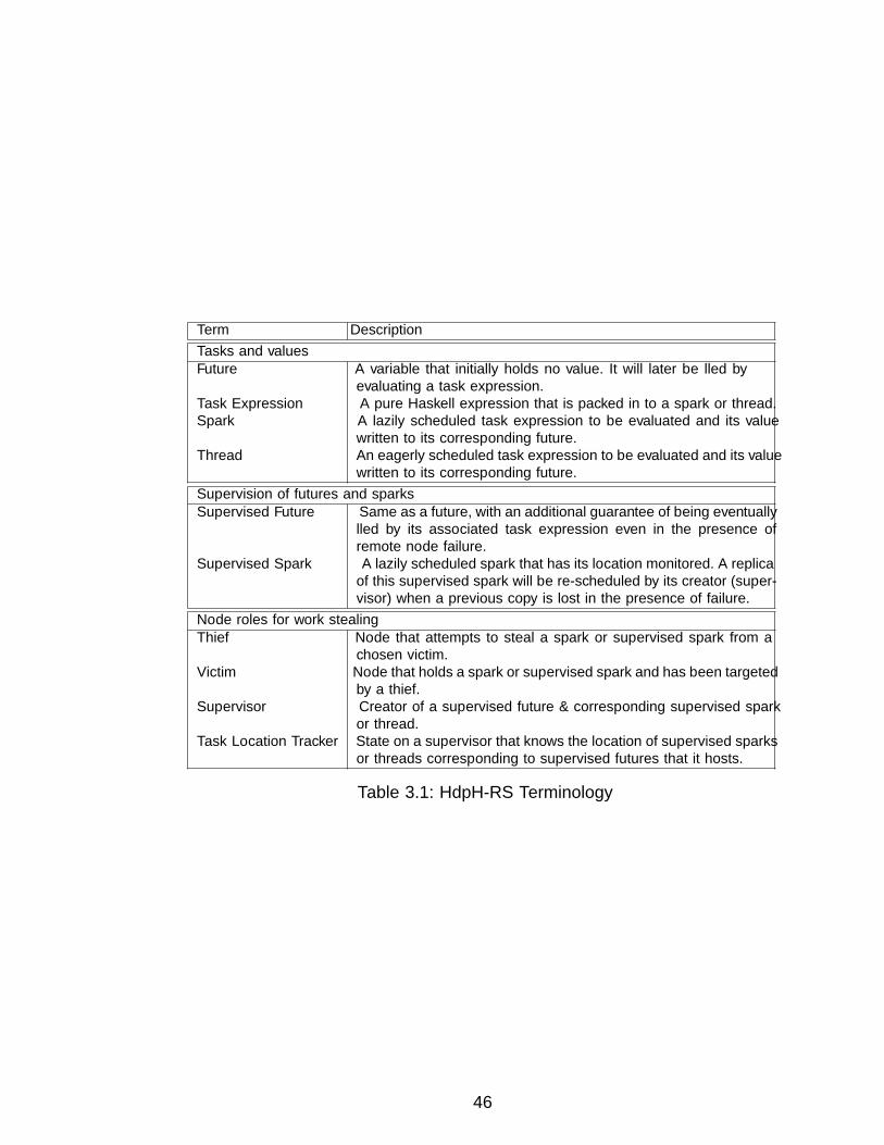
Term DescriptionTasks and valuesFuture A variable that initially holds no value. It will later be filled by

evaluating a task expression.Task Expression A pure Haskell expression that is packed in to a spark or thread.Spark A lazily scheduled task expression to be evaluated and its value

written to its corresponding future.Thread An eagerly scheduled task expression to be evaluated and its value

written to its corresponding future.Supervision of futures and sparksSupervised Future Same as a future, with an additional guarantee of being eventually

filled by its associated task expression even in the presence ofremote node failure.

Supervised Spark A lazily scheduled spark that has its location monitored. A replicaof this supervised spark will be re-scheduled by its creator (super-visor) when a previous copy is lost in the presence of failure.

Node roles for work stealingThief Node that attempts to steal a spark or supervised spark from a

chosen victim.Victim Node that holds a spark or supervised spark and has been targeted

by a thief.Supervisor Creator of a supervised future & corresponding supervised spark

or thread.Task Location Tracker State on a supervisor that knows the location of supervised sparks

or threads corresponding to supervised futures that it hosts.

Table 3.1: HdpH-RS Terminology

46

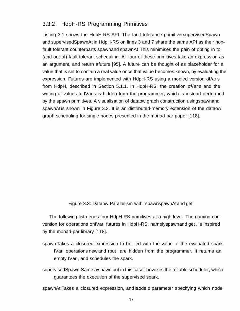
3.3.2 HdpH-RS Programming Primitives

Listing 3.1 shows the HdpH-RS API. The fault tolerance primitives supervisedSpawn

and supervisedSpawnAt in HdpH-RS on lines 3 and 7 share the same API as their non-fault tolerant counterparts spawn and spawnAt. This minimises the pain of opting in to(and out of) fault tolerant scheduling. All four of these primitives take an expression asan argument, and return a future [95]. A future can be thought of as placeholder for avalue that is set to contain a real value once that value becomes known, by evaluating theexpression. Futures are implemented with HdpH-RS using a modified version of IVarsfrom HdpH, described in Section 5.1.1. In HdpH-RS, the creation of IVars and thewriting of values to IVars is hidden from the programmer, which is instead performedby the spawn primitives. A visualisation of dataflow graph construction using spawn andspawnAt is shown in Figure 3.3. It is an distributed-memory extension of the dataflowgraph scheduling for single nodes presented in the monad-par paper [118].

f

g

h

a b

c

w x

y

Node B

Node C

Node D

Node A

km

n

j

d z

pq r

st

Parallel thread

IVar getdependence

spawn

spawnAt

Caller invokes spawn/spawnAt Sync points upon get

IVar put

Figure 3.3: Dataflow Parallelism with spawn,spawnAt and get

The following list defines four HdpH-RS primitives at a high level. The naming con-vention for operations on IVar futures in HdpH-RS, namely spawn and get, is inspiredby the monad-par library [118].

spawn Takes a closured expression to be filled with the value of the evaluated spark.IVar operations new and rput are hidden from the programmer. It returns anempty IVar, and schedules the spark.

supervisedSpawn Same as spawn, but in this case it invokes the reliable scheduler, whichguarantees the execution of the supervised spark.

spawnAt Takes a closured expression, and a NodeId parameter specifying which node

47

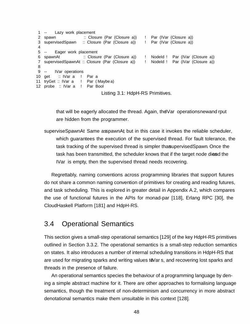
1 -- ∗ Lazy work placement2 spawn :: Closure (Par (Closure a)) → Par (IVar (Closure a))3 supervisedSpawn :: Closure (Par (Closure a)) → Par (IVar (Closure a))45 -- ∗ Eager work placement6 spawnAt :: Closure (Par (Closure a)) → NodeId → Par (IVar (Closure a))7 supervisedSpawnAt :: Closure (Par (Closure a)) → NodeId → Par (IVar (Closure a))89 -- ∗ IVar operations10 get :: IVar a → Par a11 tryGet :: IVar a → Par (Maybe a)12 probe :: IVar a → Par Bool

Listing 3.1: HdpH-RS Primitives.

that will be eagerly allocated the thread. Again, the IVar operations new and rput

are hidden from the programmer.

superviseSpawnAt Same as spawnAt, but in this case it invokes the reliable scheduler,which guarantees the execution of the supervised thread. For fault tolerance, thetask tracking of the supervised thread is simpler than supervisedSpawn. Once thetask has been transmitted, the scheduler knows that if the target node dies and theIVar is empty, then the supervised thread needs recovering.

Regrettably, naming conventions across programming libraries that support futuresdo not share a common naming convention of primitives for creating and reading futures,and task scheduling. This is explored in greater detail in Appendix A.2, which comparesthe use of functional futures in the APIs for monad-par [118], Erlang RPC [30], theCloudHaskell Platform [181] and HdpH-RS.

3.4 Operational Semantics

This section gives a small-step operational semantics [129] of the key HdpH-RS primitivesoutlined in Section 3.3.2. The operational semantics is a small-step reduction semanticson states. It also introduces a number of internal scheduling transitions in HdpH-RS thatare used for migrating sparks and writing values to IVars, and recovering lost sparks andthreads in the presence of failure.

An operational semantics specifies the behaviour of a programming language by defin-ing a simple abstract machine for it. There are other approaches to formalising languagesemantics, though the treatment of non-determinism and concurrency in more abstractdenotational semantics make them unsuitable in this context [128].

48

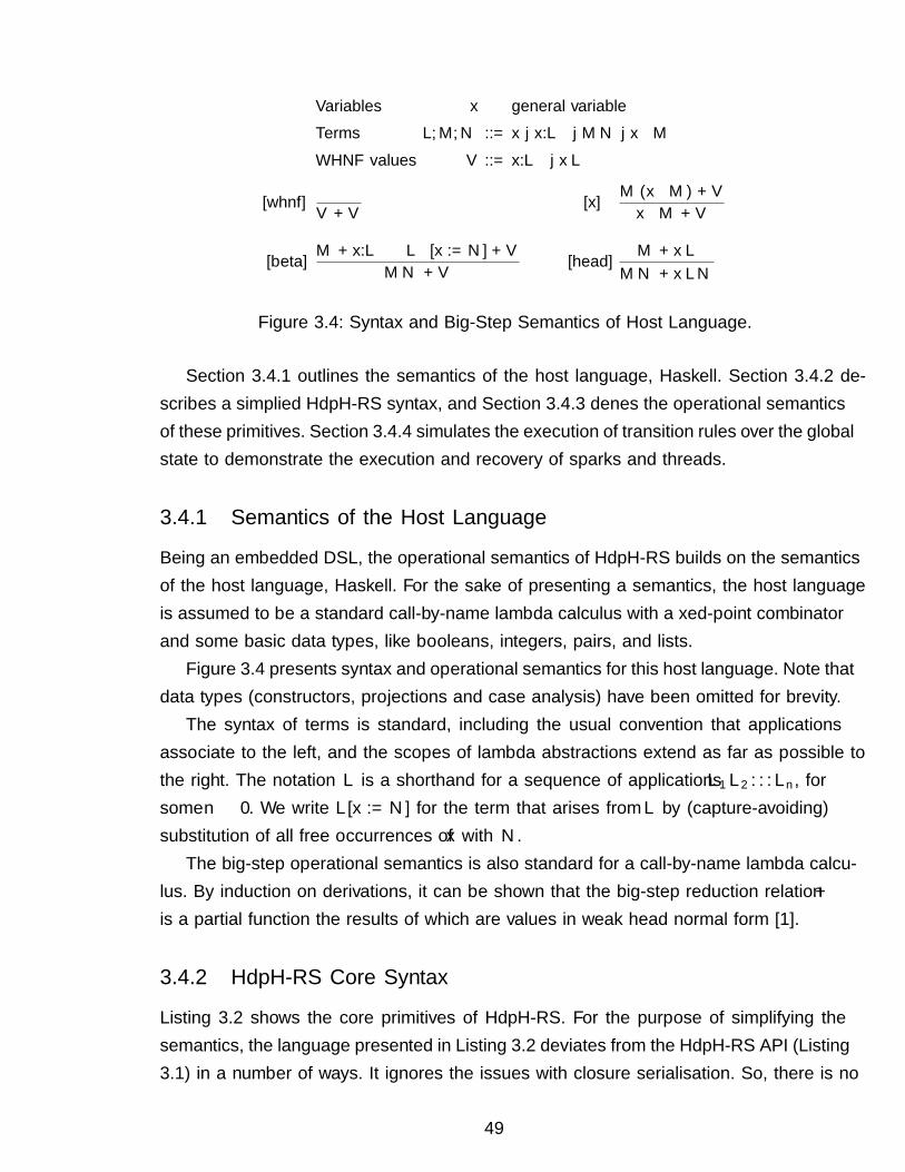
Variables x general variableTerms L,M,N ::= x | λx.L |M N | fixMWHNF values V ::= λx.L | x L̄

[whnf]V ⇓ V

[fix] M (fixM) ⇓ VfixM ⇓ V

[beta] M ⇓ λx.L L[x :=N ] ⇓ VM N ⇓ V

[head] M ⇓ x L̄M N ⇓ x L̄N

Figure 3.4: Syntax and Big-Step Semantics of Host Language.

Section 3.4.1 outlines the semantics of the host language, Haskell. Section 3.4.2 de-scribes a simplified HdpH-RS syntax, and Section 3.4.3 defines the operational semanticsof these primitives. Section 3.4.4 simulates the execution of transition rules over the globalstate to demonstrate the execution and recovery of sparks and threads.

3.4.1 Semantics of the Host Language

Being an embedded DSL, the operational semantics of HdpH-RS builds on the semanticsof the host language, Haskell. For the sake of presenting a semantics, the host languageis assumed to be a standard call-by-name lambda calculus with a fixed-point combinatorand some basic data types, like booleans, integers, pairs, and lists.

Figure 3.4 presents syntax and operational semantics for this host language. Note thatdata types (constructors, projections and case analysis) have been omitted for brevity.

The syntax of terms is standard, including the usual convention that applicationsassociate to the left, and the scopes of lambda abstractions extend as far as possible tothe right. The notation L̄ is a shorthand for a sequence of applications L1 L2 . . . Ln, forsome n ≥ 0. We write L[x := N ] for the term that arises from L by (capture-avoiding)substitution of all free occurrences of x with N .

The big-step operational semantics is also standard for a call-by-name lambda calcu-lus. By induction on derivations, it can be shown that the big-step reduction relation ⇓is a partial function the results of which are values in weak head normal form [1].

3.4.2 HdpH-RS Core Syntax

Listing 3.2 shows the core primitives of HdpH-RS. For the purpose of simplifying thesemantics, the language presented in Listing 3.2 deviates from the HdpH-RS API (Listing3.1) in a number of ways. It ignores the issues with closure serialisation. So, there is no

49

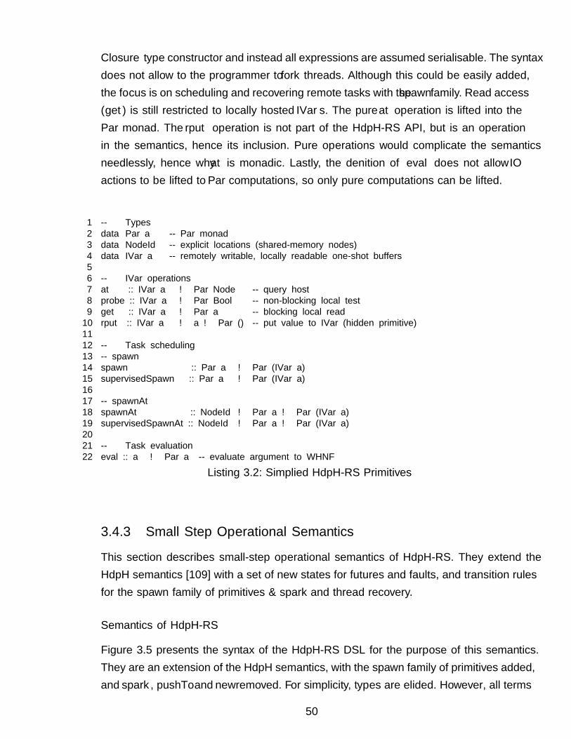
Closure type constructor and instead all expressions are assumed serialisable. The syntaxdoes not allow to the programmer to fork threads. Although this could be easily added,the focus is on scheduling and recovering remote tasks with the spawn family. Read access(get) is still restricted to locally hosted IVars. The pure at operation is lifted into thePar monad. The rput operation is not part of the HdpH-RS API, but is an operationin the semantics, hence its inclusion. Pure operations would complicate the semanticsneedlessly, hence why at is monadic. Lastly, the definition of eval does not allow IO

actions to be lifted to Par computations, so only pure computations can be lifted.

1 -- ∗ Types2 data Par a -- Par monad3 data NodeId -- explicit locations (shared-memory nodes)4 data IVar a -- remotely writable, locally readable one-shot buffers56 -- ∗ IVar operations7 at :: IVar a → Par Node -- query host8 probe :: IVar a → Par Bool -- non-blocking local test9 get :: IVar a → Par a -- blocking local read10 rput :: IVar a → a → Par () -- put value to IVar (hidden primitive)1112 -- ∗ Task scheduling13 -- spawn14 spawn :: Par a → Par (IVar a)15 supervisedSpawn :: Par a → Par (IVar a)1617 -- spawnAt18 spawnAt :: NodeId → Par a → Par (IVar a)19 supervisedSpawnAt :: NodeId → Par a → Par (IVar a)2021 -- ∗ Task evaluation22 eval :: a → Par a -- evaluate argument to WHNF

Listing 3.2: Simplified HdpH-RS Primitives

3.4.3 Small Step Operational Semantics

This section describes small-step operational semantics of HdpH-RS. They extend theHdpH semantics [109] with a set of new states for futures and faults, and transition rulesfor the spawn family of primitives & spark and thread recovery.

Semantics of HdpH-RS

Figure 3.5 presents the syntax of the HdpH-RS DSL for the purpose of this semantics.They are an extension of the HdpH semantics, with the spawn family of primitives added,and spark, pushTo and new removed. For simplicity, types are elided. However, all terms

50

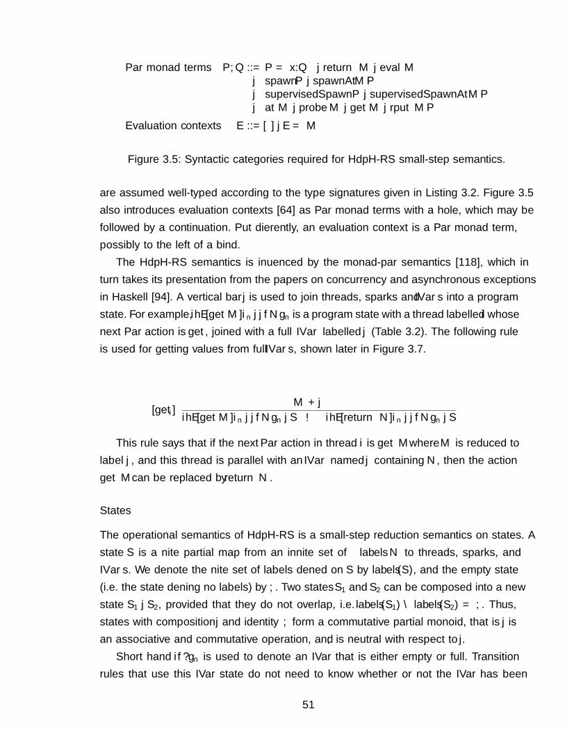
Par monad terms P,Q ::= P »= λx.Q | returnM | evalM| spawnP | spawnAtM P| supervisedSpawnP | supervisedSpawnAtM P| atM | probeM | getM | rputM P

Evaluation contexts E ::= [·] | E »=M

Figure 3.5: Syntactic categories required for HdpH-RS small-step semantics.

are assumed well-typed according to the type signatures given in Listing 3.2. Figure 3.5also introduces evaluation contexts [64] as Par monad terms with a hole, which may befollowed by a continuation. Put differently, an evaluation context is a Par monad term,possibly to the left of a bind.

The HdpH-RS semantics is influenced by the monad-par semantics [118], which inturn takes its presentation from the papers on concurrency and asynchronous exceptionsin Haskell [94]. A vertical bar | is used to join threads, sparks and IVars into a programstate. For example, i〈E [getM ]〉n | j{N}n is a program state with a thread labelled i whosenext Par action is get, joined with a full IVar labelled j (Table 3.2). The following ruleis used for getting values from full IVars, shown later in Figure 3.7.

[geti]M ⇓ j

i〈E [getM ]〉n | j{N}n | S → i〈E [returnN ]〉n | j{N}n | S

This rule says that if the next Par action in thread i is get M where M is reduced tolabel j, and this thread is parallel with an IVar named j containing N , then the actionget M can be replaced by return N.

States

The operational semantics of HdpH-RS is a small-step reduction semantics on states. Astate S is a finite partial map from an infinite set of labels N to threads, sparks, andIVars. We denote the finite set of labels defined on S by labels(S), and the empty state(i.e. the state defining no labels) by ∅. Two states S1 and S2 can be composed into a newstate S1 | S2, provided that they do not overlap, i.e. labels(S1) ∩ labels(S2) = ∅. Thus,states with composition | and identity ∅ form a commutative partial monoid, that is | isan associative and commutative operation, and ∅ is neutral with respect to |.

Short hand i{?}n is used to denote an IVar that is either empty or full. Transitionrules that use this IVar state do not need to know whether or not the IVar has been

51

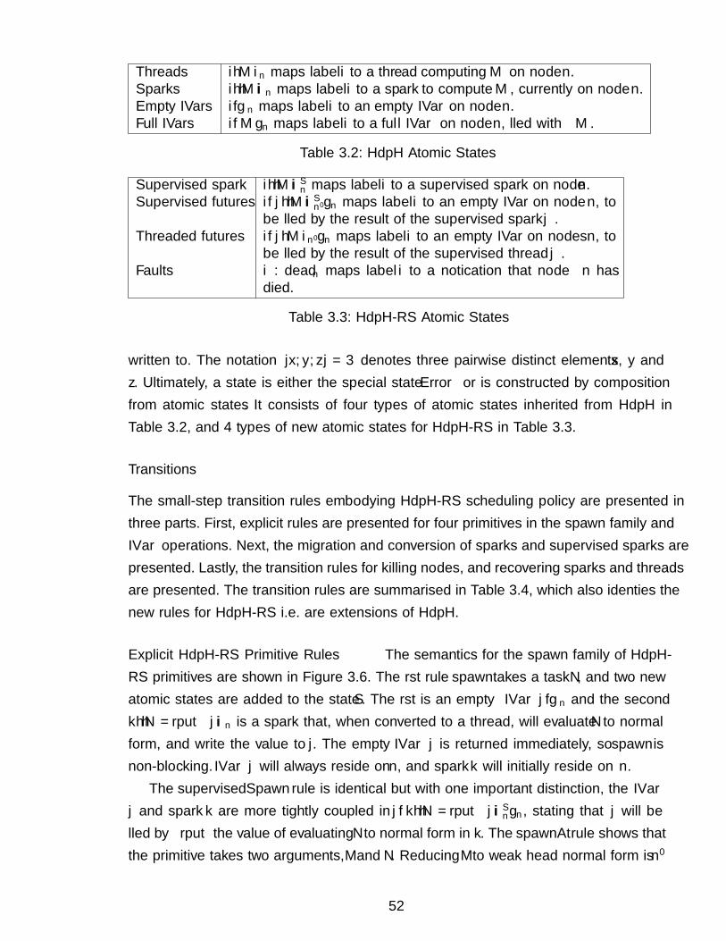
Threads i〈M〉n maps label i to a thread computing M on node n.Sparks i〈〈M〉〉n maps label i to a spark to compute M , currently on node n.Empty IVars i{}n maps label i to an empty IVar on node n.Full IVars i{M}n maps label i to a full IVar on node n, filled with M .

Table 3.2: HdpH Atomic States

Supervised spark i〈〈M〉〉Sn maps label i to a supervised spark on node n.Supervised futures i{j〈〈M〉〉Sn′}n maps label i to an empty IVar on node n, to

be filled by the result of the supervised spark j .Threaded futures i{j〈M〉n′}n maps label i to an empty IVar on nodes n, to

be filled by the result of the supervised thread j .Faults i : deadn maps label i to a notification that node n has

died.

Table 3.3: HdpH-RS Atomic States

written to. The notation |x, y, z| = 3 denotes three pairwise distinct elements x, y andz. Ultimately, a state is either the special state Error or is constructed by compositionfrom atomic states. It consists of four types of atomic states inherited from HdpH inTable 3.2, and 4 types of new atomic states for HdpH-RS in Table 3.3.

Transitions

The small-step transition rules embodying HdpH-RS scheduling policy are presented inthree parts. First, explicit rules are presented for four primitives in the spawn family andIVar operations. Next, the migration and conversion of sparks and supervised sparks arepresented. Lastly, the transition rules for killing nodes, and recovering sparks and threadsare presented. The transition rules are summarised in Table 3.4, which also identifies thenew rules for HdpH-RS i.e. are extensions of HdpH.

Explicit HdpH-RS Primitive Rules The semantics for the spawn family of HdpH-RS primitives are shown in Figure 3.6. The first rule spawn takes a task N, and two newatomic states are added to the state S. The first is an empty IVar j{}n and the secondk〈〈N »= rput j〉〉n is a spark that, when converted to a thread, will evaluate N to normalform, and write the value to j. The empty IVar j is returned immediately, so spawn isnon-blocking. IVar j will always reside on n, and spark k will initially reside on n.

The supervisedSpawn rule is identical but with one important distinction, the IVarj and spark k are more tightly coupled in j{k〈〈N »= rput j〉〉Sn}n, stating that j will befilled by rput the value of evaluating N to normal form in k. The spawnAt rule shows thatthe primitive takes two arguments, M and N. Reducing M to weak head normal form is n′

52

Transition Rules HdpH-RSExtension

Primitives & Evaluation Contexts, Figure 3.6.spawn 4supervisedSpawn 4spawnAt 4supervisedSpawnAt 4evalbindnormalizeIVar Operations, Figure 3.7.rput_emptyrput_empty_supervised_threaded_future 4rput_empty_supervised_sparked_future 4rput_fullgetget_errorprobe_emptyprobe_empty_supervised_threaded_future 4probe_empty_supervised_sparked_future 4probe_fullprobe_errorSpark Scheduling, Figure 3.8.migrate_sparkmigrate_supervised_spark 4convert_sparkconvert_supervised_spark 4

Failure & Recovery, Figure 3.9.kill_node 4kill_spark 4kill_supervised_spark 4kill_thread 4kill_ivar 4recover_supervised_spark 4recover_supervised_thread 4

Table 3.4: Summary of Transition Rules

53

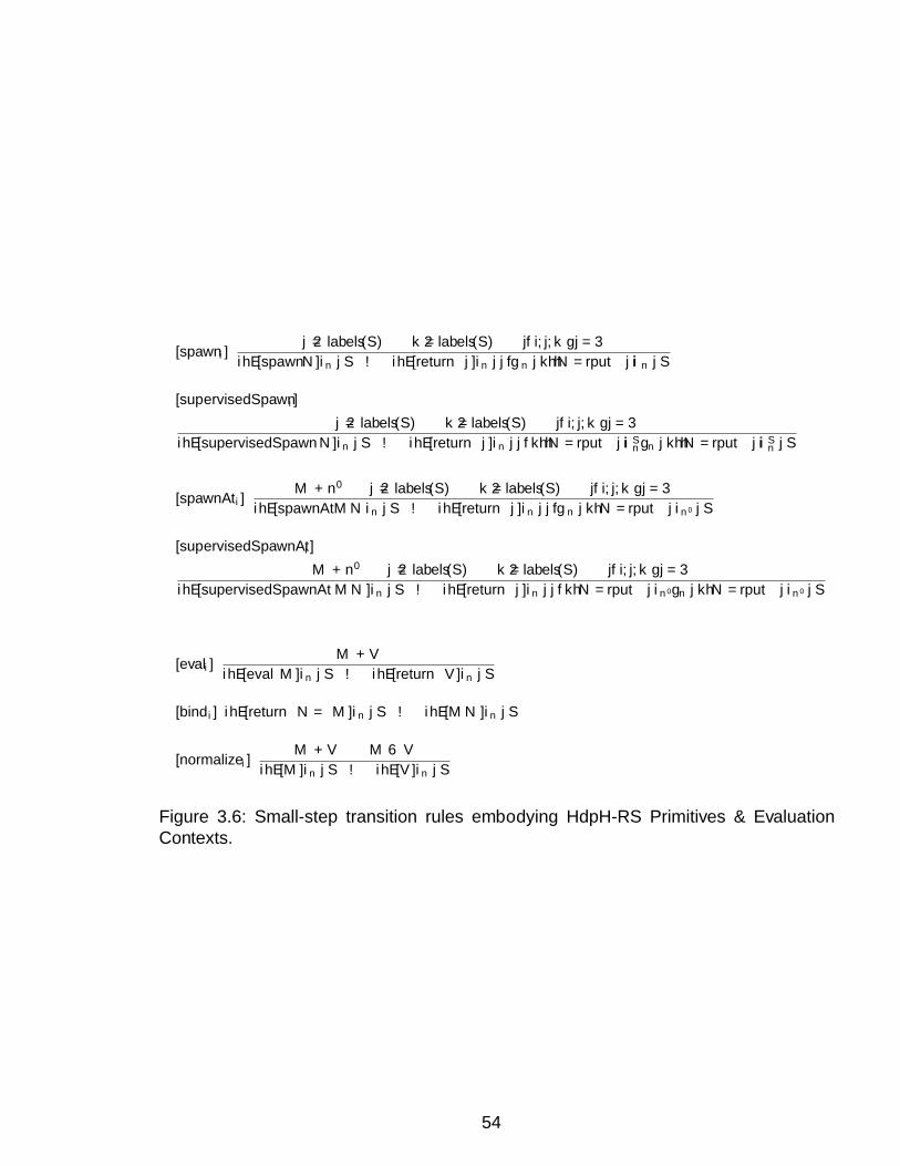
[spawni]j /∈ labels(S) k /∈ labels(S) |{i, j, k}| = 3

i〈E [spawnN ]〉n | S → i〈E [return j]〉n | j{}n | k〈〈N »= rput j〉〉n | S

[supervisedSpawni]j /∈ labels(S) k /∈ labels(S) |{i, j, k}| = 3

i〈E [supervisedSpawnN ]〉n | S → i〈E [return j]〉n | j{k〈〈N »= rput j〉〉Sn}n | k〈〈N »= rput j〉〉Sn | S

[spawnAti]M ⇓ n′ j /∈ labels(S) k /∈ labels(S) |{i, j, k}| = 3

i〈E [spawnAtM N〉n | S → i〈E [return j]〉n | j{}n | k〈N »= rput j〉n′ | S

[supervisedSpawnAti]M ⇓ n′ j /∈ labels(S) k /∈ labels(S) |{i, j, k}| = 3

i〈E [supervisedSpawnAtM N ]〉n | S → i〈E [return j]〉n | j{k〈N »= rput j〉n′}n | k〈N »= rput j〉n′ | S

[evali]M ⇓ V

i〈E [evalM ]〉n | S → i〈E [returnV ]〉n | S

[bindi] i〈E [returnN »=M ]〉n | S → i〈E [M N ]〉n | S

[normalizei]M ⇓ V M 6≡ V

i〈E [M ]〉n | S → i〈E [V ]〉n | S

Figure 3.6: Small-step transition rules embodying HdpH-RS Primitives & EvaluationContexts.

54

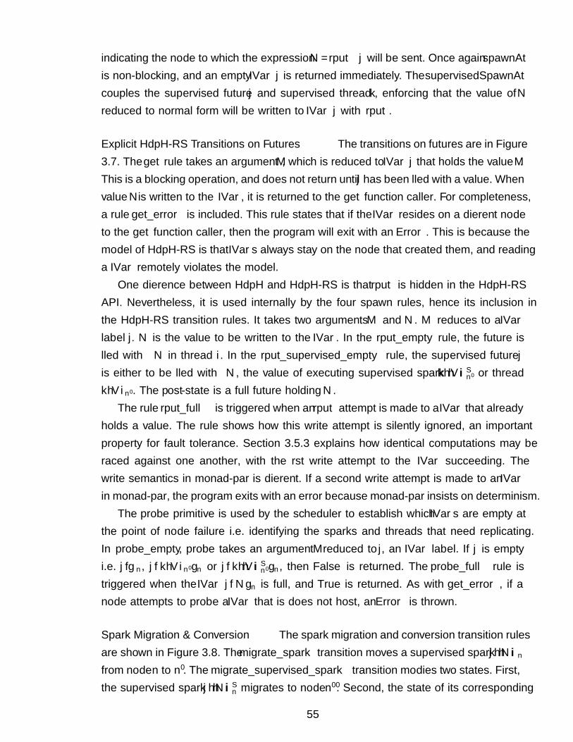
indicating the node to which the expression N »=rput j will be sent. Once again spawnAt

is non-blocking, and an empty IVar j is returned immediately. The supervisedSpawnAtcouples the supervised future j and supervised thread k, enforcing that the value of Nreduced to normal form will be written to IVar j with rput.

Explicit HdpH-RS Transitions on Futures The transitions on futures are in Figure3.7. The get rule takes an argument M, which is reduced to IVar j that holds the value M.This is a blocking operation, and does not return until j has been filled with a value. Whenvalue N is written to the IVar, it is returned to the get function caller. For completeness,a rule get_error is included. This rule states that if the IVar resides on a different nodeto the get function caller, then the program will exit with an Error. This is because themodel of HdpH-RS is that IVars always stay on the node that created them, and readinga IVar remotely violates the model.

One difference between HdpH and HdpH-RS is that rput is hidden in the HdpH-RSAPI. Nevertheless, it is used internally by the four spawn rules, hence its inclusion inthe HdpH-RS transition rules. It takes two arguments M and N . M reduces to a IVar

label j. N is the value to be written to the IVar. In the rput_empty rule, the future isfilled with N in thread i. In the rput_supervised_empty rule, the supervised future jis either to be filled with N , the value of executing supervised spark k〈〈V 〉〉Sn′ or threadk〈V 〉n′ . The post-state is a full future holding N .

The rule rput_full is triggered when an rput attempt is made to a IVar that alreadyholds a value. The rule shows how this write attempt is silently ignored, an importantproperty for fault tolerance. Section 3.5.3 explains how identical computations may beraced against one another, with the first write attempt to the IVar succeeding. Thewrite semantics in monad-par is different. If a second write attempt is made to an IVar

in monad-par, the program exits with an error because monad-par insists on determinism.The probe primitive is used by the scheduler to establish which IVars are empty at

the point of node failure i.e. identifying the sparks and threads that need replicating.In probe_empty, probe takes an argument M reduced to j, an IVar label. If j is emptyi.e. j{}n, j{k〈V 〉n′}n or j{k〈〈V 〉〉Sn′}n, then False is returned. The probe_full rule istriggered when the IVar j{N}n is full, and True is returned. As with get_error, if anode attempts to probe a IVar that is does not host, an Error is thrown.

Spark Migration & Conversion The spark migration and conversion transition rulesare shown in Figure 3.8. The migrate_spark transition moves a supervised spark j〈〈N〉〉nfrom node n to n′. The migrate_supervised_spark transition modifies two states. First,the supervised spark j〈〈N〉〉Sn migrates to node n′′. Second, the state of its corresponding

55

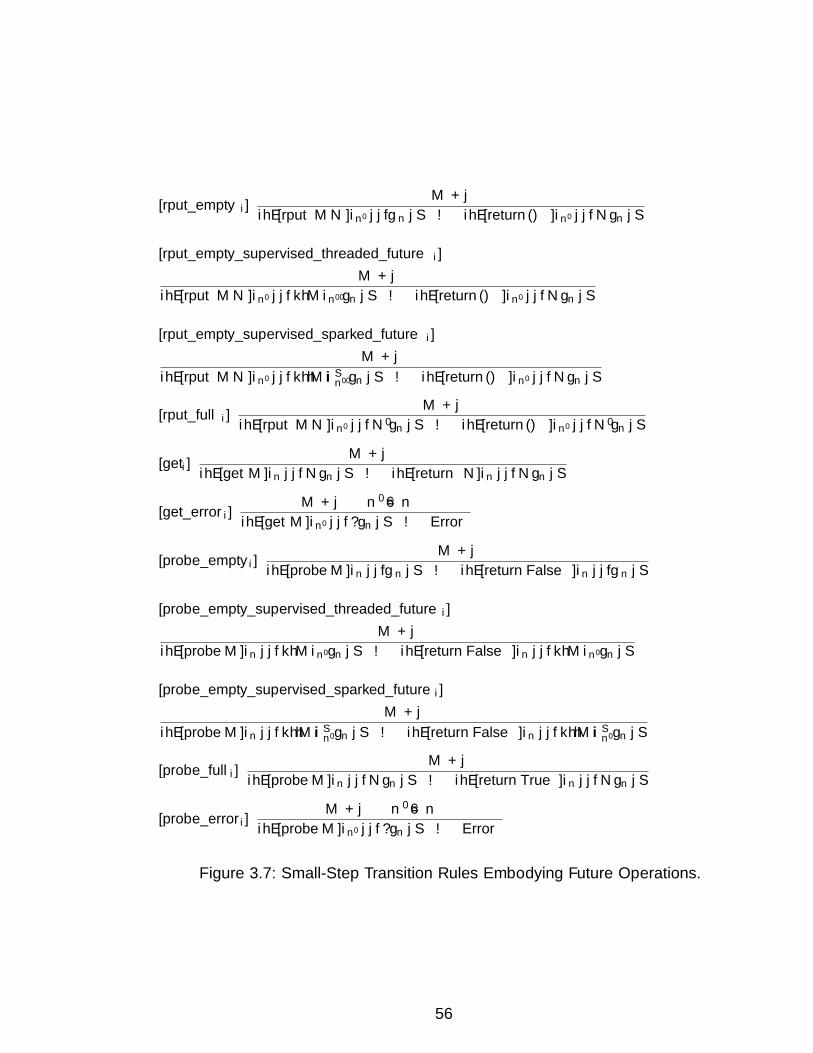
[rput_emptyi]M ⇓ j

i〈E [rputM N ]〉n′ | j{}n | S → i〈E [return ()]〉n′ | j{N}n | S

[rput_empty_supervised_threaded_futurei]M ⇓ j

i〈E [rputM N ]〉n′ | j{k〈M〉n′′}n | S → i〈E [return ()]〉n′ | j{N}n | S

[rput_empty_supervised_sparked_futurei]M ⇓ j

i〈E [rputM N ]〉n′ | j{k〈〈M〉〉Sn′′}n | S → i〈E [return ()]〉n′ | j{N}n | S

[rput_fulli]M ⇓ j

i〈E [rputM N ]〉n′ | j{N ′}n | S → i〈E [return ()]〉n′ | j{N ′}n | S

[geti]M ⇓ j

i〈E [getM ]〉n | j{N}n | S → i〈E [returnN ]〉n | j{N}n | S

[get_errori]M ⇓ j n′ 6= n

i〈E [getM ]〉n′ | j{?}n | S → Error

[probe_emptyi]M ⇓ j

i〈E [probeM ]〉n | j{}n | S → i〈E [return False]〉n | j{}n | S

[probe_empty_supervised_threaded_futurei]M ⇓ j

i〈E [probeM ]〉n | j{k〈M〉n′}n | S → i〈E [return False]〉n | j{k〈M〉n′}n | S

[probe_empty_supervised_sparked_futurei]M ⇓ j

i〈E [probeM ]〉n | j{k〈〈M〉〉Sn′}n | S → i〈E [return False]〉n | j{k〈〈M〉〉Sn′}n | S

[probe_fulli]M ⇓ j

i〈E [probeM ]〉n | j{N}n | S → i〈E [return True]〉n | j{N}n | S

[probe_errori]M ⇓ j n′ 6= n

i〈E [probeM ]〉n′ | j{?}n | S → Error

Figure 3.7: Small-Step Transition Rules Embodying Future Operations.

56

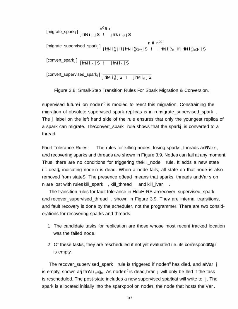
[migrate_sparkj ]n′ 6= n

j〈〈N〉〉n | S → j〈〈N〉〉n′ | S

[migrate_supervised_sparkj ]n 6= n′′

j〈〈N〉〉Sn | i{j〈〈N〉〉Sn}n′ | S → j〈〈N〉〉Sn′′ | i{j〈〈N〉〉Sn′′}n | S

[convert_sparkj ]j〈〈M〉〉n | S → j〈M〉n | S

[convert_supervised_sparkj ]j〈〈M〉〉Sn | S → j〈M〉n | S

Figure 3.8: Small-Step Transition Rules For Spark Migration & Conversion.

supervised future i on node n′ is modified to reflect this migration. Constraining themigration of obsolete supervised spark replicas is in rule migrate_supervised_spark.The j label on the left hand side of the rule ensures that only the youngest replica ofa spark can migrate. The convert_spark rule shows that the spark j is converted to athread.

Fault Tolerance Rules The rules for killing nodes, losing sparks, threads and IVars,and recovering sparks and threads are shown in Figure 3.9. Nodes can fail at any moment.Thus, there are no conditions for triggering the kill_node rule. It adds a new statei : deadn indicating node n is dead. When a node fails, all state on that node is alsoremoved from state S. The presence of deadn means that sparks, threads and IVars onn are lost with rules kill_spark, kill_thread and kill_ivar.

The transition rules for fault tolerance in HdpH-RS are recover_supervised_sparkand recover_supervised_thread, shown in Figure 3.9. They are internal transitions,and fault recovery is done by the scheduler, not the programmer. There are two consid-erations for recovering sparks and threads.

1. The candidate tasks for replication are those whose most recent tracked locationwas the failed node.

2. Of these tasks, they are rescheduled if not yet evaluated i.e. its corresponding IVar

is empty.

The recover_supervised_spark rule is triggered if node n′ has died, and a IVar jis empty, shown as j{〈〈N〉〉n′}n. As node n′ is dead, IVar j will only be filled if the taskis rescheduled. The post-state includes a new supervised spark k that will write to j. Thespark is allocated initially into the sparkpool on node n, the node that hosts the IVar.

57

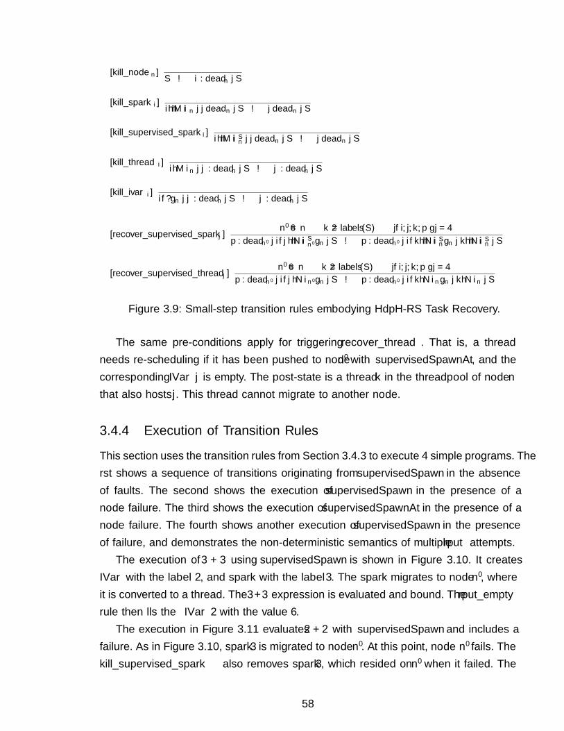
[kill_noden]S → i : deadn | S

[kill_sparki]i〈〈M〉〉n | j deadn | S → j deadn | S

[kill_supervised_sparki]i〈〈M〉〉Sn | j deadn | S → j deadn | S

[kill_threadi]i〈M〉n | j : deadn | S → j : deadn | S

[kill_ivari]i{?}n | j : deadn | S → j : deadn | S

[recover_supervised_sparkj ]n′ 6= n k /∈ labels(S) |{i, j, k, p}| = 4

p : deadn′ | i{j〈〈N〉〉Sn′}n | S → p : deadn′ | i{k〈〈N〉〉Sn}n | k〈〈N〉〉Sn | S

[recover_supervised_threadj ]n′ 6= n k /∈ labels(S) |{i, j, k, p}| = 4

p : deadn′ | i{j〈N〉n′}n | S → p : deadn′ | i{k〈N〉n}n | k〈N〉n | S

Figure 3.9: Small-step transition rules embodying HdpH-RS Task Recovery.

The same pre-conditions apply for triggering recover_thread. That is, a threadneeds re-scheduling if it has been pushed to node n′ with supervisedSpawnAt, and thecorresponding IVar j is empty. The post-state is a thread k in the threadpool of node nthat also hosts j. This thread cannot migrate to another node.

3.4.4 Execution of Transition Rules

This section uses the transition rules from Section 3.4.3 to execute 4 simple programs. Thefirst shows a sequence of transitions originating from supervisedSpawn in the absenceof faults. The second shows the execution of supervisedSpawn in the presence of anode failure. The third shows the execution of supervisedSpawnAt in the presence of anode failure. The fourth shows another execution of supervisedSpawn in the presenceof failure, and demonstrates the non-deterministic semantics of multiple rput attempts.

The execution of 3 + 3 using supervisedSpawn is shown in Figure 3.10. It createsIVar with the label 2, and spark with the label 3. The spark migrates to node n′, whereit is converted to a thread. The 3+3 expression is evaluated and bound. The rput_emptyrule then fills the IVar 2 with the value 6.

The execution in Figure 3.11 evaluates 2 + 2 with supervisedSpawn and includes afailure. As in Figure 3.10, spark 3 is migrated to node n′. At this point, node n′ fails. Thekill_supervised_spark also removes spark 3, which resided on n′ when it failed. The

58

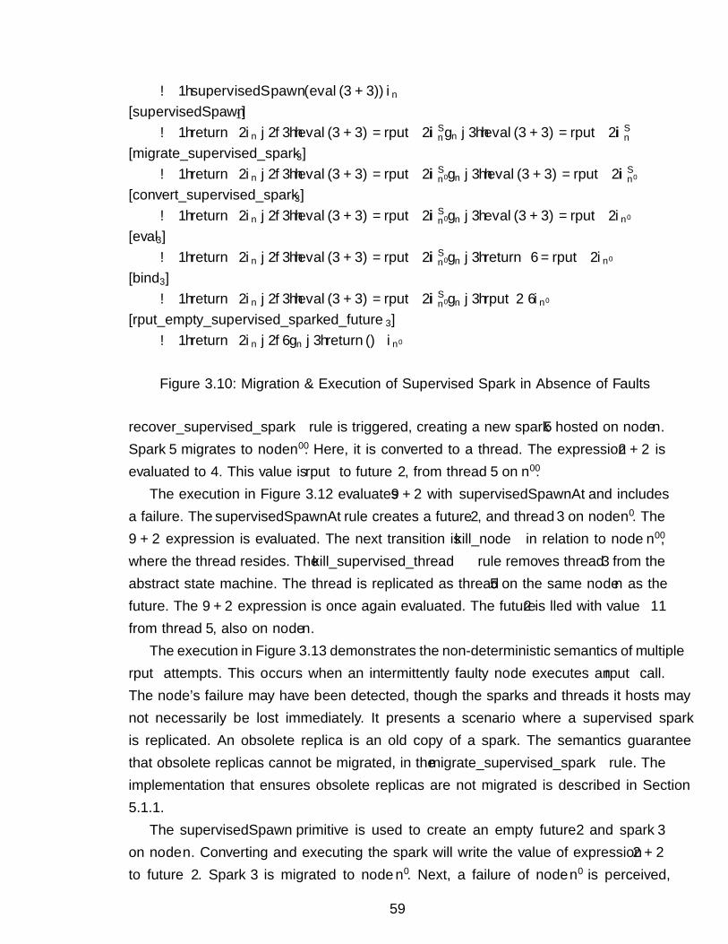
→ 1〈supervisedSpawn (eval (3 + 3))〉n[supervisedSpawn1]

→ 1〈return 2〉n | 2{3〈〈eval (3 + 3) »= rput 2〉〉Sn}n | 3〈〈eval (3 + 3) »= rput 2〉〉Sn[migrate_supervised_spark3]

→ 1〈return 2〉n | 2{3〈〈eval (3 + 3) »= rput 2〉〉Sn′}n | 3〈〈eval (3 + 3) »= rput 2〉〉Sn′

[convert_supervised_spark3]→ 1〈return 2〉n | 2{3〈〈eval (3 + 3) »= rput 2〉〉Sn′}n | 3〈eval (3 + 3) »= rput 2〉n′

[eval3]→ 1〈return 2〉n | 2{3〈〈eval (3 + 3) »= rput 2〉〉Sn′}n | 3〈return 6 »= rput 2〉n′

[bind3]→ 1〈return 2〉n | 2{3〈〈eval (3 + 3) »= rput 2〉〉Sn′}n | 3〈rput 2 6〉n′

[rput_empty_supervised_sparked_future3]→ 1〈return 2〉n | 2{6}n | 3〈return ()〉n′

Figure 3.10: Migration & Execution of Supervised Spark in Absence of Faults

recover_supervised_spark rule is triggered, creating a new spark 5 hosted on node n.Spark 5 migrates to node n′′. Here, it is converted to a thread. The expression 2 + 2 isevaluated to 4. This value is rput to future 2, from thread 5 on n′′.

The execution in Figure 3.12 evaluates 9 + 2 with supervisedSpawnAt and includesa failure. The supervisedSpawnAt rule creates a future 2, and thread 3 on node n′. The9 + 2 expression is evaluated. The next transition is kill_node in relation to node n′′,where the thread resides. The kill_supervised_thread rule removes thread 3 from theabstract state machine. The thread is replicated as thread 5 on the same node n as thefuture. The 9 + 2 expression is once again evaluated. The future 2 is filled with value 11from thread 5, also on node n.

The execution in Figure 3.13 demonstrates the non-deterministic semantics of multiplerput attempts. This occurs when an intermittently faulty node executes an rput call.The node’s failure may have been detected, though the sparks and threads it hosts maynot necessarily be lost immediately. It presents a scenario where a supervised sparkis replicated. An obsolete replica is an old copy of a spark. The semantics guaranteethat obsolete replicas cannot be migrated, in the migrate_supervised_spark rule. Theimplementation that ensures obsolete replicas are not migrated is described in Section5.1.1.

The supervisedSpawn primitive is used to create an empty future 2 and spark 3on node n. Converting and executing the spark will write the value of expression 2 + 2to future 2. Spark 3 is migrated to node n′. Next, a failure of node n′ is perceived,

59

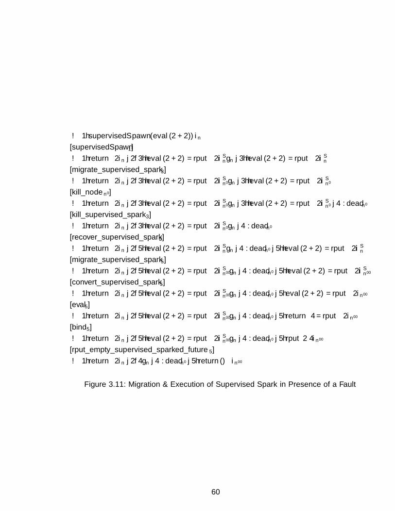
→ 1〈supervisedSpawn (eval (2 + 2))〉n[supervisedSpawn1]→ 1〈return 2〉n | 2{3〈〈eval (2 + 2) »= rput 2〉〉Sn}n | 3〈〈eval (2 + 2) »= rput 2〉〉Sn[migrate_supervised_spark3]→ 1〈return 2〉n | 2{3〈〈eval (2 + 2) »= rput 2〉〉Sn′}n | 3〈〈eval (2 + 2) »= rput 2〉〉Sn′

[kill_noden′ ]→ 1〈return 2〉n | 2{3〈〈eval (2 + 2) »= rput 2〉〉Sn′}n | 3〈〈eval (2 + 2) »= rput 2〉〉Sn′ | 4 : deadn′

[kill_supervised_spark3]→ 1〈return 2〉n | 2{3〈〈eval (2 + 2) »= rput 2〉〉Sn′}n | 4 : deadn′

[recover_supervised_spark3]→ 1〈return 2〉n | 2{5〈〈eval (2 + 2) »= rput 2〉〉Sn}n | 4 : deadn′ | 5〈〈eval (2 + 2) »= rput 2〉〉Sn[migrate_supervised_spark5]→ 1〈return 2〉n | 2{5〈〈eval (2 + 2) »= rput 2〉〉Sn′′}n | 4 : deadn′ | 5〈〈eval (2 + 2) »= rput 2〉〉Sn′′

[convert_supervised_spark5]→ 1〈return 2〉n | 2{5〈〈eval (2 + 2) »= rput 2〉〉Sn′′}n | 4 : deadn′ | 5〈eval (2 + 2) »= rput 2〉n′′

[eval5]→ 1〈return 2〉n | 2{5〈〈eval (2 + 2) »= rput 2〉〉Sn′′}n | 4 : deadn′ | 5〈return 4 »= rput 2〉n′′

[bind5]→ 1〈return 2〉n | 2{5〈〈eval (2 + 2) »= rput 2〉〉Sn′′}n | 4 : deadn′ | 5〈rput 2 4〉n′′

[rput_empty_supervised_sparked_future5]→ 1〈return 2〉n | 2{4}n | 4 : deadn′ | 5〈return ()〉n′′

Figure 3.11: Migration & Execution of Supervised Spark in Presence of a Fault

60

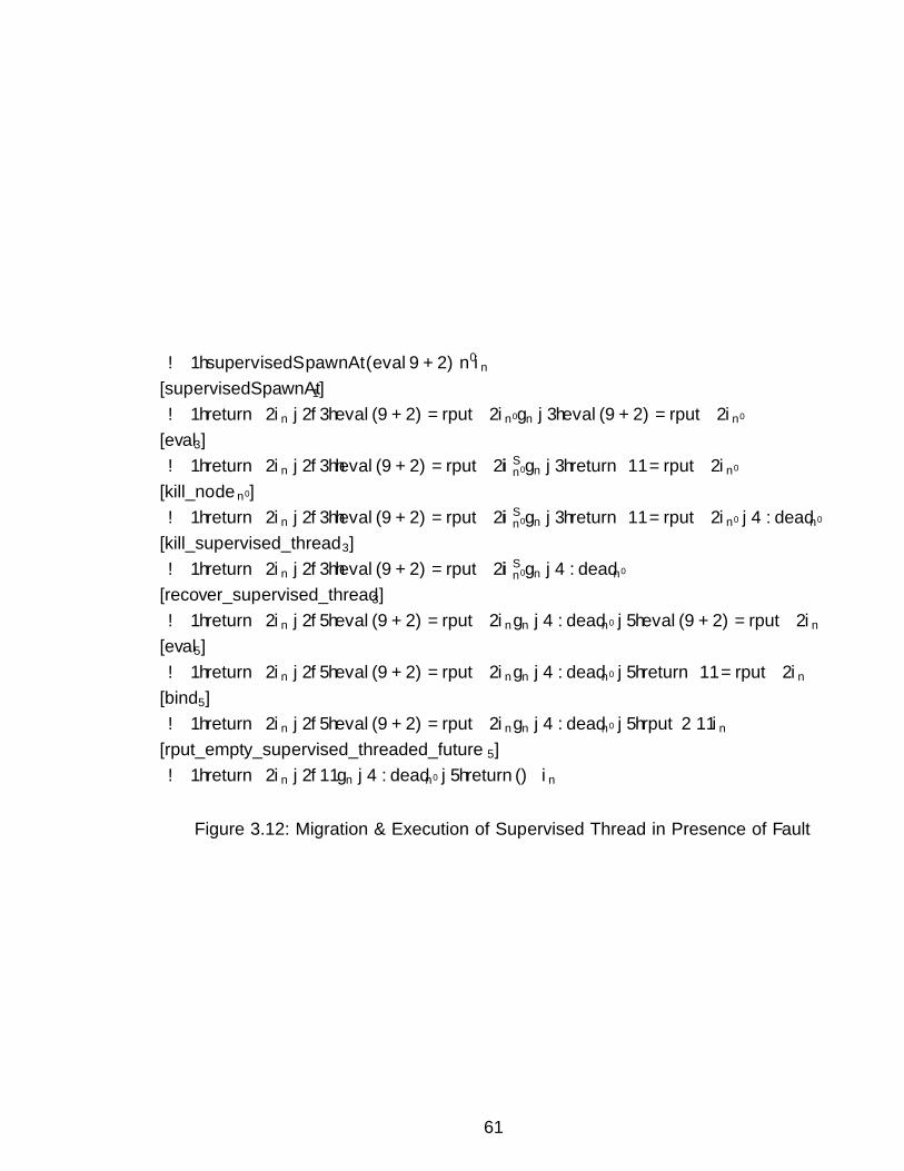
→ 1〈supervisedSpawnAt (eval 9 + 2) n′〉n[supervisedSpawnAt1]→ 1〈return 2〉n | 2{3〈eval (9 + 2) »= rput 2〉n′}n | 3〈eval (9 + 2) »= rput 2〉n′

[eval3]→ 1〈return 2〉n | 2{3〈〈eval (9 + 2) »= rput 2〉〉Sn′}n | 3〈return 11 »= rput 2〉n′

[kill_noden′ ]→ 1〈return 2〉n | 2{3〈〈eval (9 + 2) »= rput 2〉〉Sn′}n | 3〈return 11 »= rput 2〉n′ | 4 : deadn′

[kill_supervised_thread3]→ 1〈return 2〉n | 2{3〈〈eval (9 + 2) »= rput 2〉〉Sn′}n | 4 : deadn′

[recover_supervised_thread3]→ 1〈return 2〉n | 2{5〈eval (9 + 2) »= rput 2〉n}n | 4 : deadn′ | 5〈eval (9 + 2) »= rput 2〉n[eval5]→ 1〈return 2〉n | 2{5〈eval (9 + 2) »= rput 2〉n}n | 4 : deadn′ | 5〈return 11 »= rput 2〉n[bind5]→ 1〈return 2〉n | 2{5〈eval (9 + 2) »= rput 2〉n}n | 4 : deadn′ | 5〈rput 2 11〉n[rput_empty_supervised_threaded_future5]→ 1〈return 2〉n | 2{11}n | 4 : deadn′ | 5〈return ()〉n

Figure 3.12: Migration & Execution of Supervised Thread in Presence of Fault

61

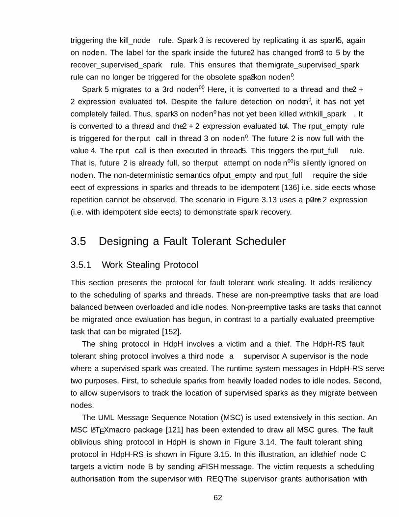
triggering the kill_node rule. Spark 3 is recovered by replicating it as spark 5, againon node n. The label for the spark inside the future 2 has changed from 3 to 5 by therecover_supervised_spark rule. This ensures that the migrate_supervised_spark

rule can no longer be triggered for the obsolete spark 3 on node n′.Spark 5 migrates to a 3rd node n′′. Here, it is converted to a thread and the 2 +

2 expression evaluated to 4. Despite the failure detection on node n′, it has not yetcompletely failed. Thus, spark 3 on node n′ has not yet been killed with kill_spark. Itis converted to a thread and the 2 + 2 expression evaluated to 4. The rput_empty ruleis triggered for the rput call in thread 3 on node n′. The future 2 is now full with thevalue 4. The rput call is then executed in thread 5. This triggers the rput_full rule.That is, future 2 is already full, so the rput attempt on node n′′ is silently ignored onnode n. The non-deterministic semantics of rput_empty and rput_full require the sideeffect of expressions in sparks and threads to be idempotent [136] i.e. side effects whoserepetition cannot be observed. The scenario in Figure 3.13 uses a pure 2 + 2 expression(i.e. with idempotent side effects) to demonstrate spark recovery.

3.5 Designing a Fault Tolerant Scheduler

3.5.1 Work Stealing Protocol

This section presents the protocol for fault tolerant work stealing. It adds resiliencyto the scheduling of sparks and threads. These are non-preemptive tasks that are loadbalanced between overloaded and idle nodes. Non-preemptive tasks are tasks that cannotbe migrated once evaluation has begun, in contrast to a partially evaluated preemptivetask that can be migrated [152].

The fishing protocol in HdpH involves a victim and a thief. The HdpH-RS faulttolerant fishing protocol involves a third node — a supervisor. A supervisor is the nodewhere a supervised spark was created. The runtime system messages in HdpH-RS servetwo purposes. First, to schedule sparks from heavily loaded nodes to idle nodes. Second,to allow supervisors to track the location of supervised sparks as they migrate betweennodes.

The UML Message Sequence Notation (MSC) is used extensively in this section. AnMSC LATEXmacro package [121] has been extended to draw all MSC figures. The faultoblivious fishing protocol in HdpH is shown in Figure 3.14. The fault tolerant fishingprotocol in HdpH-RS is shown in Figure 3.15. In this illustration, an idle thief node Ctargets a victim node B by sending a FISH message. The victim requests a schedulingauthorisation from the supervisor with REQ. The supervisor grants authorisation with

62

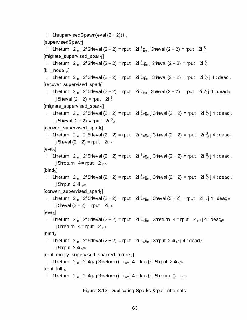
→ 1〈supervisedSpawn (eval (2 + 2))〉n[supervisedSpawn1]→ 1〈return 2〉n | 2{3〈〈eval (2 + 2) »= rput 2〉〉Sn}n | 3〈〈eval (2 + 2) »= rput 2〉〉Sn

[migrate_supervised_spark3]→ 1〈return 2〉n | 2{3〈〈eval (2 + 2) »= rput 2〉〉Sn′}n | 3〈〈eval (2 + 2) »= rput 2〉〉Sn′

[kill_noden′ ]→ 1〈return 2〉n | 2{3〈〈eval (2 + 2) »= rput 2〉〉Sn′}n | 3〈〈eval (2 + 2) »= rput 2〉〉Sn′ | 4 : deadn′

[recover_supervised_spark3]→ 1〈return 2〉n | 2{5〈〈eval (2 + 2) »= rput 2〉〉Sn}n | 3〈〈eval (2 + 2) »= rput 2〉〉Sn′ | 4 : deadn′

| 5〈〈eval (2 + 2) »= rput 2〉〉Sn[migrate_supervised_spark5]→ 1〈return 2〉n | 2{5〈〈eval (2 + 2) »= rput 2〉〉Sn′′}n | 3〈〈eval (2 + 2) »= rput 2〉〉Sn′ | 4 : deadn′

| 5〈〈eval (2 + 2) »= rput 2〉〉Sn′′

[convert_supervised_spark5]→ 1〈return 2〉n | 2{5〈〈eval (2 + 2) »= rput 2〉〉Sn′′}n | 3〈〈eval (2 + 2) »= rput 2〉〉Sn′ | 4 : deadn′

| 5〈eval (2 + 2) »= rput 2〉n′′

[eval5]→ 1〈return 2〉n | 2{5〈〈eval (2 + 2) »= rput 2〉〉Sn′′}n | 3〈〈eval (2 + 2) »= rput 2〉〉Sn′ | 4 : deadn′

| 5〈return 4 »= rput 2〉n′′

[bind5]→ 1〈return 2〉n | 2{5〈〈eval (2 + 2) »= rput 2〉〉Sn′′}n | 3〈〈eval (2 + 2) »= rput 2〉〉Sn′ | 4 : deadn′

| 5〈rput 2 4〉n′′

[convert_supervised_spark3]→ 1〈return 2〉n | 2{5〈〈eval (2 + 2) »= rput 2〉〉Sn′′}n | 3〈eval (2 + 2) »= rput 2〉n′ | 4 : deadn′

| 5〈eval (2 + 2) »= rput 2〉n′′

[eval3]→ 1〈return 2〉n | 2{5〈〈eval (2 + 2) »= rput 2〉〉Sn′′}n | 3〈return 4 »= rput 2〉n′ | 4 : deadn′

| 5〈return 4 »= rput 2〉n′′

[bind3]→ 1〈return 2〉n | 2{5〈〈eval (2 + 2) »= rput 2〉〉Sn′′}n | 3〈rput 2 4〉n′ | 4 : deadn′

| 5〈rput 2 4〉n′′

[rput_empty_supervised_sparked_future3]→ 1〈return 2〉n | 2{4}n | 3〈return ()〉n′ | 4 : deadn′ | 5〈rput 2 4〉n′′

[rput_full5]→ 1〈return 2〉n | 2{4}n | 3〈return ()〉n′ | 4 : deadn′ | 5〈return ()〉n′′

Figure 3.13: Duplicating Sparks & rput Attempts

63

AUTH, and a spark is scheduled from the victim to the thief in a SCHEDULE message.When the thief receives this, it sends an ACK to the supervisor.

Node A Node Bvictim

Node Cthief

FISH

SCHEDULE

Figure 3.14: Fault Oblivious Fishing Protocol in HdpH

Node Asupervisor

Node Bvictim

Node Cthief

FISHREQ

AUTHSCHEDULE

ACK

Figure 3.15: Fault Tolerant Fishing Protocol in HdpH-RS

RTS Messages to Support the Work Stealing Protocol

The HdpH-RS RTS messages are described in Table 3.5. The Message header is themessage type, the From and To fields distinguish a supervisor node (S) and worker nodes(W), and Description shows the purpose of the message. The use of each message aredescribed in the scheduling algorithms in Section 3.5.4.

3.5.2 Task Locality

For the supervisor to determine whether a spark is lost when a remote node has failed,the migration of a supervised spark needs to be tracked. This is made possible from theRTS messages REQ and ACK described in Section 5.5.3.

Task migration tracking is in shown in Figure 3.16. The messages REQ and ACK arereceived by the supervising node A to keep track of a spark’s location. Sparks and threadscan therefore be identified by their corresponding globalised IVar. If a spark is createdwith supervisedSpawn, then the supervised spark’s structure is composed of three parts.First, an identifier corresponding the IVar that will be filled by evaluating the taskexpression in the spark. Second, a replica number of the spark. Third, the task expressioninside the spark to be evaluated. In Figure 3.16 the IVar is represented as iX e.g. i2, and

64

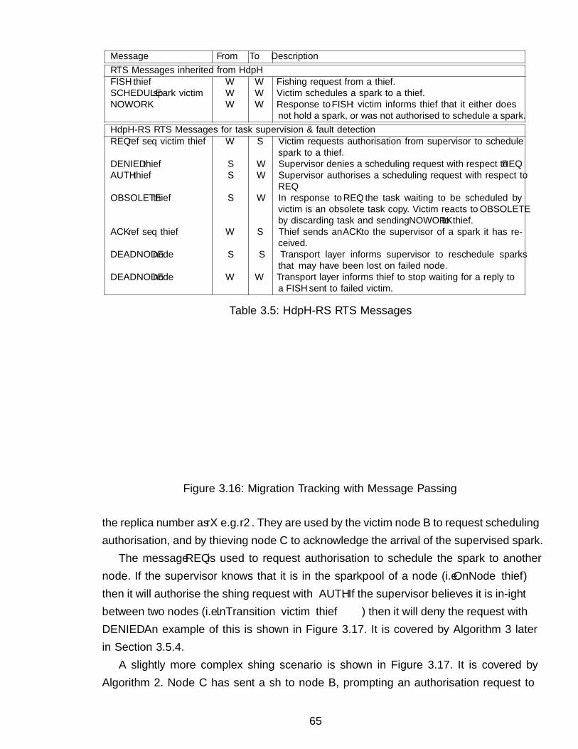
Message From To DescriptionRTS Messages inherited from HdpHFISH thief W W Fishing request from a thief.SCHEDULE spark victim W W Victim schedules a spark to a thief.NOWORK W W Response to FISH: victim informs thief that it either does

not hold a spark, or was not authorised to schedule a spark.HdpH-RS RTS Messages for task supervision & fault detectionREQ ref seq victim thief W S Victim requests authorisation from supervisor to schedule

spark to a thief.DENIED thief S W Supervisor denies a scheduling request with respect to REQ.AUTH thief S W Supervisor authorises a scheduling request with respect to

REQ.OBSOLETE thief S W In response to REQ: the task waiting to be scheduled by

victim is an obsolete task copy. Victim reacts to OBSOLETEby discarding task and sending NOWORK to thief.

ACK ref seq thief W S Thief sends an ACK to the supervisor of a spark it has re-ceived.

DEADNODE node S S Transport layer informs supervisor to reschedule sparksthat may have been lost on failed node.

DEADNODE node W W Transport layer informs thief to stop waiting for a reply toa FISH sent to failed victim.

Table 3.5: HdpH-RS RTS Messages

Node Asupervisor

Node Bvictim

Node Cthief

OnNode Bholds ..0

FISH CREQ i0 r0 B C

AUTH C

InTransition B CSCHEDULE ..0 B

ACK i0 r0 C

OnNode C

Figure 3.16: Migration Tracking with Message Passing

the replica number as rX e.g. r2. They are used by the victim node B to request schedulingauthorisation, and by thieving node C to acknowledge the arrival of the supervised spark.

The message REQ is used to request authorisation to schedule the spark to anothernode. If the supervisor knows that it is in the sparkpool of a node (i.e. OnNode thief)then it will authorise the fishing request with AUTH. If the supervisor believes it is in-flightbetween two nodes (i.e. InTransition victim thief) then it will deny the request withDENIED. An example of this is shown in Figure 3.17. It is covered by Algorithm 3 laterin Section 3.5.4.

A slightly more complex fishing scenario is shown in Figure 3.17. It is covered byAlgorithm 2. Node C has sent a fish to node B, prompting an authorisation request to

65

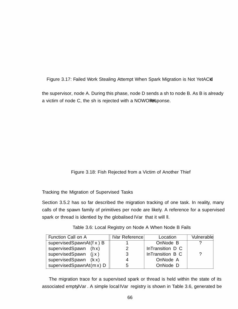
Node Asupervisor

Node Bvictim

Node Cthief1

Node Dthief2

holds ..0InTransition B C

SCHEDULE ..0 BFISH D

REQ i0 r0 C D

DENIED DNOWORK

ACK i0 r0 C

OnNode C

Figure 3.17: Failed Work Stealing Attempt When Spark Migration is Not Yet ACKd

the supervisor, node A. During this phase, node D sends a fish to node B. As B is alreadya victim of node C, the fish is rejected with a NOWORK response.

Node Asupervisor

Node Bworker

Node Cworker

Node Dworker

holds ..0OnNode B

FISH CREQ i0 r0 B C

FISH D

NOWORKAUTH C

InTransition B CSCHEDULE ..0 B

ACK i0 r0 C

OnNode C

Figure 3.18: Fish Rejected from a Victim of Another Thief

Tracking the Migration of Supervised Tasks

Section 3.5.2 has so far described the migration tracking of one task. In reality, manycalls of the spawn family of primitives per node are likely. A reference for a supervisedspark or thread is identified by the globalised IVar that it will fill.

Table 3.6: Local Registry on Node A When Node B Fails

Function Call on A IVar Reference Location VulnerablesupervisedSpawnAt (f x) B 1 OnNode B ?supervisedSpawn (hx) 2 InTransition D CsupervisedSpawn (j x) 3 InTransition B C ?supervisedSpawn (k x) 4 OnNode AsupervisedSpawnAt (mx) D 5 OnNode D

The migration trace for a supervised spark or thread is held within the state of itsassociated empty IVar. A simple local IVar registry is shown in Table 3.6, generated be

66

1 -- | Par computation that generates registry entries in Table 3.62 foo :: Int → Par Integer3 foo x = do4 ivar1 ← supervisedSpawnAt $(mkClosure [ | f x |]) nodeB5 ivar2 ← supervisedSpawn $(mkClosure [ | h x |])6 ivar2 ← supervisedSpawn $(mkClosure [ | j x |])7 ivar2 ← supervisedSpawn $(mkClosure [ | k x |])8 ivar2 ← supervisedSpawnAt $(mkClosure [ | m x |]) nodeD9 x ← get ivar110 y ← get ivar211 {- omitted -}

Listing 3.3: Par Computation That Modifies Local Registry on Node A

executing the code fragment in Listing 3.3 is executed on node A. Five futures (IVars)have been created on node A. Node A expects REQ and ACK messages about each futureit supervises, from victims and thieves respectively. The registry is used to identify whichsparks and threads need recovering. Table 3.6 shows which tasks are at-risk when thefailure of node B is detected by node A. If node A receives a DEADNODE B message fromthe transport layer, the tasks for IVars 1 and 3 are replicated. The replication of task3 may lead to duplicate copies if it has arrived at node C before node B failed. Themanagement of duplicate sparks is described in Section 3.5.3.

Fishing Hops

The HdpH scheduler supports fishing hops, but the HdpH-RS scheduler does not. Hopsallow a thief to scrutinise a number of potential victim targets for work, before it givesup and attempts again after a random delay. A thief will transmit a fish message to arandom target. If that target does not have sparks to offer, the victim will forward thefish on behalf of the thief. Each fish request is given a maximum hop count. That is, thenumber of times it will be forwarded before a NOWORK message is returned to the thief.

Idle nodes proactively fish for sparks on other nodes. When they send a fish, they donot send another until they receive a reply from a targeted node. The expected reply isSCHEDULE with a spark, or NOWORK. Algorithm 10 shows how a node will stop waiting fora reply when a DEADNODE message is received about the chosen victim.

If hops were supported, thieves may potentially be deadlocked while waiting for afishing reply. A simple scenario is shown in Figure 3.19. A spark is fished from node Ato B. Node D sends a fish to C, which is forwarded to node B. Node B receives the fish,but fails before sending a reply to D. Although D will receive a DEADNODE B message, itwill not reset the fishing lock. It is expecting a reply from C, and is oblivious to the fact

67

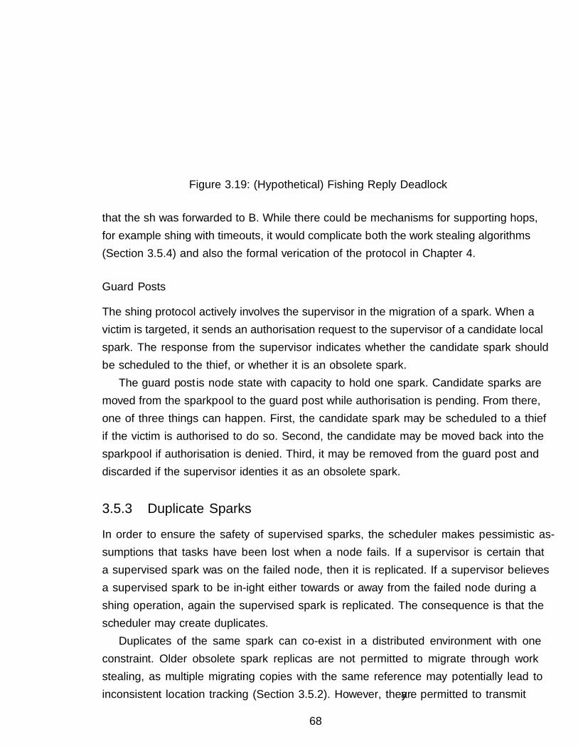
Node Asupervisor

Node Bvictim

Node Cthief1

Node Dthief2

OnNode A

SCHEDULE ..0 A

InTransition A BFISH hop1 C

FISH hop2 C

DEADNODE Bdeadlock

Figure 3.19: (Hypothetical) Fishing Reply Deadlock

that the fish was forwarded to B. While there could be mechanisms for supporting hops,for example fishing with timeouts, it would complicate both the work stealing algorithms(Section 3.5.4) and also the formal verification of the protocol in Chapter 4.

Guard Posts

The fishing protocol actively involves the supervisor in the migration of a spark. When avictim is targeted, it sends an authorisation request to the supervisor of a candidate localspark. The response from the supervisor indicates whether the candidate spark shouldbe scheduled to the thief, or whether it is an obsolete spark.

The guard post is node state with capacity to hold one spark. Candidate sparks aremoved from the sparkpool to the guard post while authorisation is pending. From there,one of three things can happen. First, the candidate spark may be scheduled to a thiefif the victim is authorised to do so. Second, the candidate may be moved back into thesparkpool if authorisation is denied. Third, it may be removed from the guard post anddiscarded if the supervisor identifies it as an obsolete spark.

3.5.3 Duplicate Sparks

In order to ensure the safety of supervised sparks, the scheduler makes pessimistic as-sumptions that tasks have been lost when a node fails. If a supervisor is certain thata supervised spark was on the failed node, then it is replicated. If a supervisor believesa supervised spark to be in-flight either towards or away from the failed node during afishing operation, again the supervised spark is replicated. The consequence is that thescheduler may create duplicates.

Duplicates of the same spark can co-exist in a distributed environment with oneconstraint. Older obsolete spark replicas are not permitted to migrate through workstealing, as multiple migrating copies with the same reference may potentially lead toinconsistent location tracking (Section 3.5.2). However, they are permitted to transmit

68

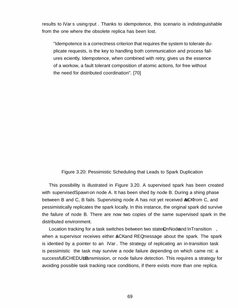
results to IVars using rput. Thanks to idempotence, this scenario is indistinguishablefrom the one where the obsolete replica has been lost.

"Idempotence is a correctness criterion that requires the system to tolerate du-plicate requests, is the key to handling both communication and process fail-ures efficiently. Idempotence, when combined with retry, gives us the essenceof a workflow, a fault tolerant composition of atomic actions, for free withoutthe need for distributed coordination". [70]

Node Asupervisor

Node Bvictim

Node Cthief1

Node Dthief2

OnNode B holds ..0 FISH C

REQ r0 s0 B C

AUTH C

InTransition B CSCHEDULE ..0 B

holds ..0DEADNODE B

create replica ..1FISH D

REQ r0 s1 A DAUTH D

SCHEDULE ..1 A

holds ..1

Figure 3.20: Pessimistic Scheduling that Leads to Spark Duplication

This possibility is illustrated in Figure 3.20. A supervised spark has been createdwith supervisedSpawn on node A. It has been fished by node B. During a fishing phasebetween B and C, B fails. Supervising node A has not yet received an ACK from C, andpessimistically replicates the spark locally. In this instance, the original spark did survivethe failure of node B. There are now two copies of the same supervised spark in thedistributed environment.

Location tracking for a task switches between two states, OnNode and InTransition,when a supervisor receives either a ACK and REQ message about the spark. The sparkis identified by a pointer to an IVar. The strategy of replicating an in-transition taskis pessimistic — the task may survive a node failure depending on which came first: asuccessful SCHEDULE transmission, or node failure detection. This requires a strategy foravoiding possible task tracking race conditions, if there exists more than one replica.

69

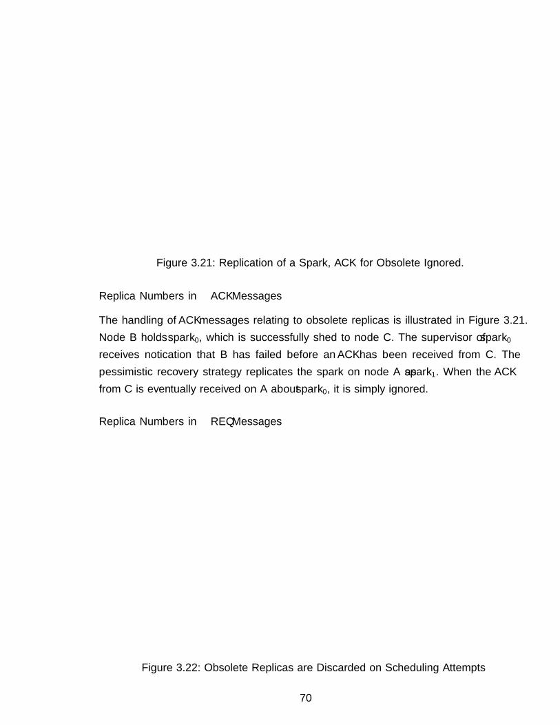
Node Asupervisor

Node Bvictim

Node Cthief

holds ..0OnNode B

FISH C

REQ i0 r0 B C

AUTH C

InTransition B CSCHEDULE ..0 B

DEADNODE B

create replica ..1

OnNode A

ACK i0 r0 C

ACK for ..0 ignored

Figure 3.21: Replication of a Spark, ACK for Obsolete Ignored.

Replica Numbers in ACK Messages

The handling of ACK messages relating to obsolete replicas is illustrated in Figure 3.21.Node B holds spark0, which is successfully fished to node C. The supervisor of spark0

receives notification that B has failed before an ACK has been received from C. Thepessimistic recovery strategy replicates the spark on node A as spark1. When the ACK

from C is eventually received on A about spark0, it is simply ignored.

Replica Numbers in REQ Messages

Node Asupervisor

Node Bvictim

Node Cthief1

Node Dthief2

holds ..2holds ..3

OnNode AFISH D

REQ i0 r3 A DAUTH D

SCHEDULE ..3 A

InTransition A D FISH Cholds ..3

REQ i0 r2 B C

OBSOLETE C

NOWORK

discards ..2ACK i0 r3 D

OnNode D

Figure 3.22: Obsolete Replicas are Discarded on Scheduling Attempts

70

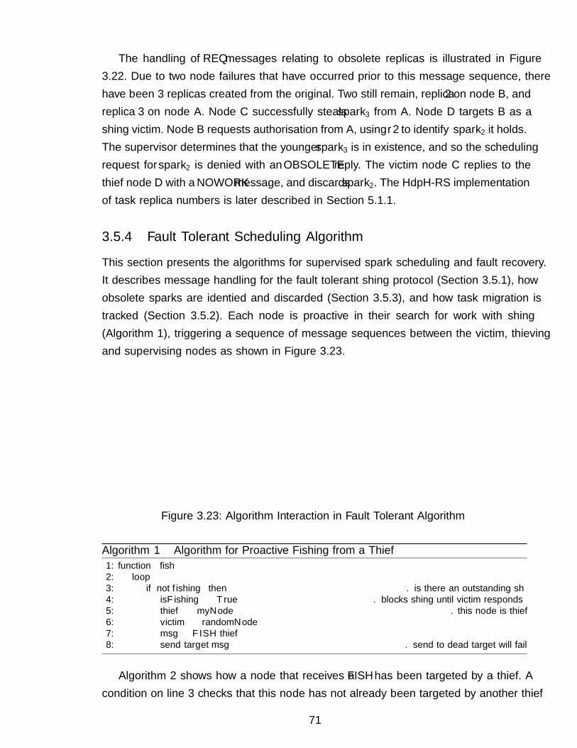
The handling of REQ messages relating to obsolete replicas is illustrated in Figure3.22. Due to two node failures that have occurred prior to this message sequence, therehave been 3 replicas created from the original. Two still remain, replica 2 on node B, andreplica 3 on node A. Node C successfully steals spark3 from A. Node D targets B as afishing victim. Node B requests authorisation from A, using r2 to identify spark2 it holds.The supervisor determines that the younger spark3 is in existence, and so the schedulingrequest for spark2 is denied with an OBSOLETE reply. The victim node C replies to thethief node D with a NOWORK message, and discards spark2. The HdpH-RS implementationof task replica numbers is later described in Section 5.1.1.

3.5.4 Fault Tolerant Scheduling Algorithm

This section presents the algorithms for supervised spark scheduling and fault recovery.It describes message handling for the fault tolerant fishing protocol (Section 3.5.1), howobsolete sparks are identified and discarded (Section 3.5.3), and how task migration istracked (Section 3.5.2). Each node is proactive in their search for work with fishing(Algorithm 1), triggering a sequence of message sequences between the victim, thievingand supervising nodes as shown in Figure 3.23.

REQ

NOWORK

NOWORK

NOWORK

8

5

2

3

4

9

OBSOLETE

DENIED

FISH

1

6

ACK

7

= AlgorithmN N

AUTH

SCHEDULE

Figure 3.23: Algorithm Interaction in Fault Tolerant Algorithm

Algorithm 1 Algorithm for Proactive Fishing from a Thief1: function fish2: loop3: if not fishing then . is there an outstanding fish4: isF ishing ← True . blocks fishing until victim responds5: thief ← myNode . this node is thief6: victim← randomNode7: msg ← FISH thief8: send target msg . send to dead target will fail

Algorithm 2 shows how a node that receives a FISH has been targeted by a thief. Acondition on line 3 checks that this node has not already been targeted by another thief

71

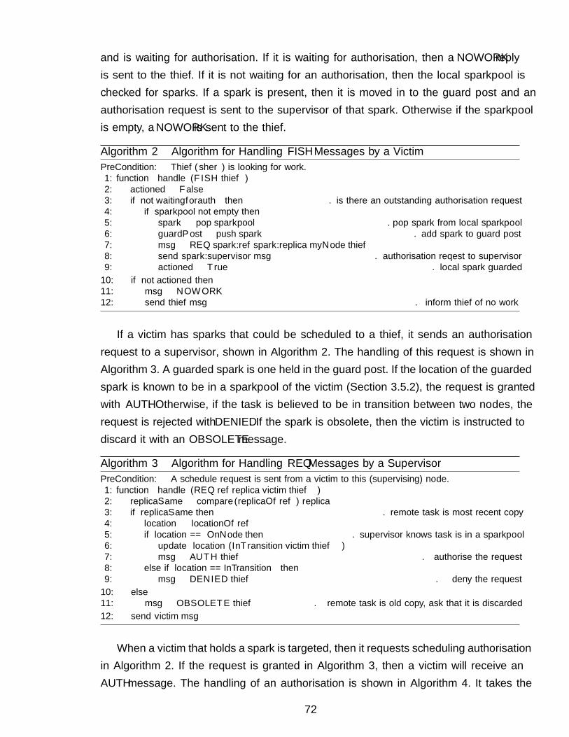
and is waiting for authorisation. If it is waiting for authorisation, then a NOWORK replyis sent to the thief. If it is not waiting for an authorisation, then the local sparkpool ischecked for sparks. If a spark is present, then it is moved in to the guard post and anauthorisation request is sent to the supervisor of that spark. Otherwise if the sparkpoolis empty, a NOWORK is sent to the thief.

Algorithm 2 Algorithm for Handling FISH Messages by a VictimPreCondition: Thief (fisher) is looking for work.1: function handle(FISH thief)2: actioned← False3: if not waitingforauth then . is there an outstanding authorisation request4: if sparkpool not empty then5: spark ← pop sparkpool . pop spark from local sparkpool6: guardPost← push spark . add spark to guard post7: msg ← REQ spark.ref spark.replica myNode thief8: send spark.supervisor msg . authorisation reqest to supervisor9: actioned← True . local spark guarded10: if not actioned then11: msg ← NOWORK12: send thief msg . inform thief of no work

If a victim has sparks that could be scheduled to a thief, it sends an authorisationrequest to a supervisor, shown in Algorithm 2. The handling of this request is shown inAlgorithm 3. A guarded spark is one held in the guard post. If the location of the guardedspark is known to be in a sparkpool of the victim (Section 3.5.2), the request is grantedwith AUTH. Otherwise, if the task is believed to be in transition between two nodes, therequest is rejected with DENIED. If the spark is obsolete, then the victim is instructed todiscard it with an OBSOLETE message.

Algorithm 3 Algorithm for Handling REQ Messages by a SupervisorPreCondition: A schedule request is sent from a victim to this (supervising) node.1: function handle(REQ ref replica victim thief)2: replicaSame← compare (replicaOf ref) replica3: if replicaSame then . remote task is most recent copy4: location← locationOf ref5: if location == OnNode then . supervisor knows task is in a sparkpool6: update location (InTransition victim thief)7: msg ← AUTH thief . authorise the request8: else if location == InTransition then9: msg ← DENIED thief . deny the request10: else11: msg ← OBSOLETE thief . remote task is old copy, ask that it is discarded12: send victim msg

When a victim that holds a spark is targeted, then it requests scheduling authorisationin Algorithm 2. If the request is granted in Algorithm 3, then a victim will receive anAUTH message. The handling of an authorisation is shown in Algorithm 4. It takes the

72

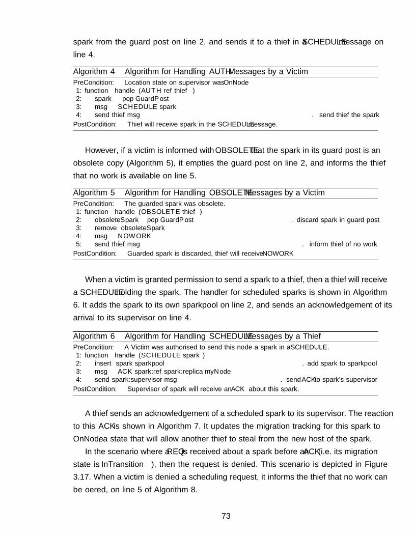
spark from the guard post on line 2, and sends it to a thief in a SCHEDULE message online 4.

Algorithm 4 Algorithm for Handling AUTH Messages by a VictimPreCondition: Location state on supervisor was OnNode.1: function handle(AUTH ref thief)2: spark ← pop GuardPost3: msg ← SCHEDULE spark4: send thief msg . send thief the sparkPostCondition: Thief will receive spark in the SCHEDULE message.

However, if a victim is informed with OBSOLETE that the spark in its guard post is anobsolete copy (Algorithm 5), it empties the guard post on line 2, and informs the thiefthat no work is available on line 5.

Algorithm 5 Algorithm for Handling OBSOLETE Messages by a VictimPreCondition: The guarded spark was obsolete.1: function handle(OBSOLETE thief)2: obsoleteSpark ← pop GuardPost . discard spark in guard post3: remove obsoleteSpark4: msg ← NOWORK5: send thief msg . inform thief of no workPostCondition: Guarded spark is discarded, thief will receive NOWORK.

When a victim is granted permission to send a spark to a thief, then a thief will receivea SCHEDULE holding the spark. The handler for scheduled sparks is shown in Algorithm6. It adds the spark to its own sparkpool on line 2, and sends an acknowledgement of itsarrival to its supervisor on line 4.

Algorithm 6 Algorithm for Handling SCHEDULE Messages by a ThiefPreCondition: A Victim was authorised to send this node a spark in a SCHEDULE.1: function handle(SCHEDULE spark)2: insert spark sparkpool . add spark to sparkpool3: msg ← ACK spark.ref spark.replica myNode4: send spark.supervisor msg . send ACK to spark’s supervisorPostCondition: Supervisor of spark will receive an ACK about this spark.

A thief sends an acknowledgement of a scheduled spark to its supervisor. The reactionto this ACK is shown in Algorithm 7. It updates the migration tracking for this spark toOnNode, a state that will allow another thief to steal from the new host of the spark.

In the scenario where a REQ is received about a spark before an ACK (i.e. its migrationstate is InTransition), then the request is denied. This scenario is depicted in Figure3.17. When a victim is denied a scheduling request, it informs the thief that no work canbe offered, on line 5 of Algorithm 8.

73

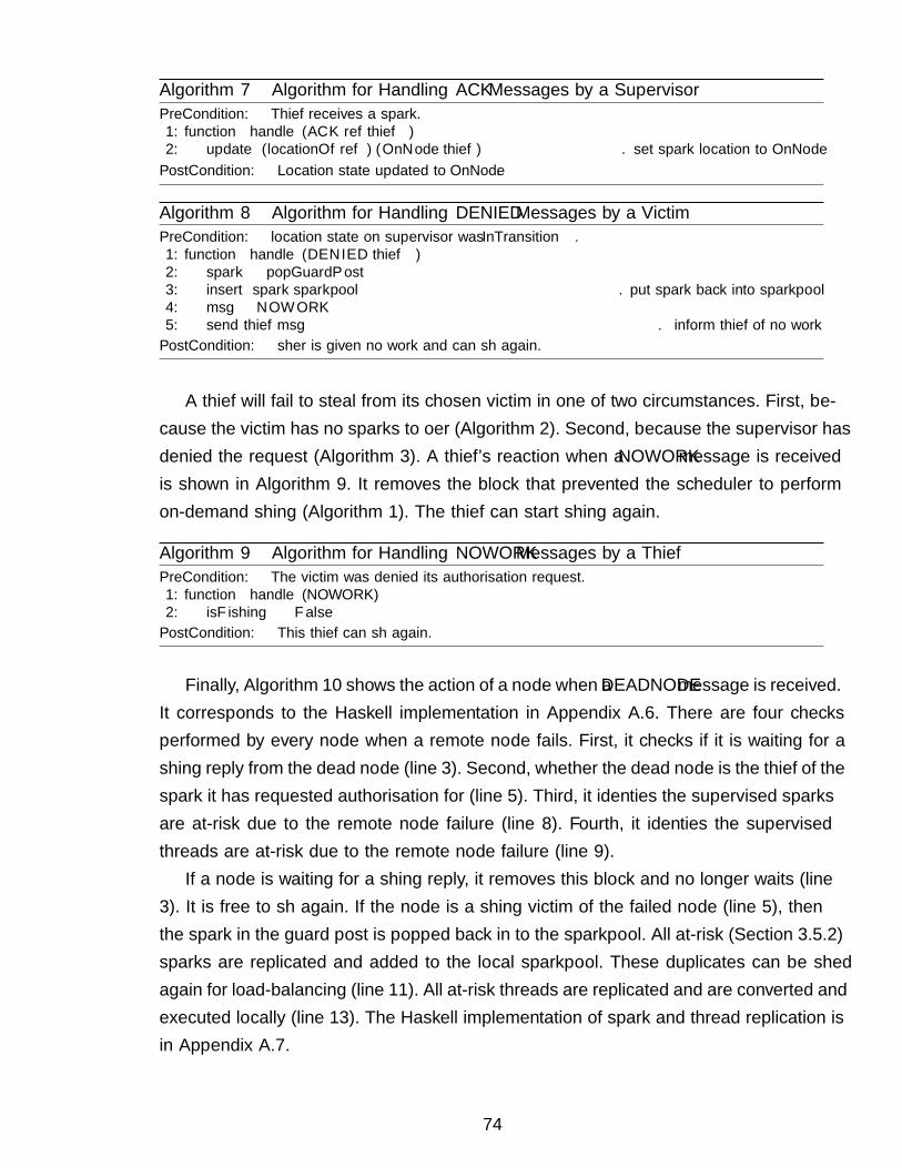
Algorithm 7 Algorithm for Handling ACK Messages by a SupervisorPreCondition: Thief receives a spark.1: function handle(ACK ref thief)2: update (locationOf ref) (OnNode thief) . set spark location to OnNodePostCondition: Location state updated to OnNode.

Algorithm 8 Algorithm for Handling DENIED Messages by a VictimPreCondition: location state on supervisor was InTransition.1: function handle(DENIED thief)2: spark ← popGuardPost3: insert spark sparkpool . put spark back into sparkpool4: msg ← NOWORK5: send thief msg . inform thief of no workPostCondition: fisher is given no work and can fish again.

A thief will fail to steal from its chosen victim in one of two circumstances. First, be-cause the victim has no sparks to offer (Algorithm 2). Second, because the supervisor hasdenied the request (Algorithm 3). A thief’s reaction when a NOWORK message is receivedis shown in Algorithm 9. It removes the block that prevented the scheduler to performon-demand fishing (Algorithm 1). The thief can start fishing again.

Algorithm 9 Algorithm for Handling NOWORK Messages by a ThiefPreCondition: The victim was denied its authorisation request.1: function handle(NOWORK)2: isF ishing ← False

PostCondition: This thief can fish again.

Finally, Algorithm 10 shows the action of a node when a DEADNODEmessage is received.It corresponds to the Haskell implementation in Appendix A.6. There are four checksperformed by every node when a remote node fails. First, it checks if it is waiting for afishing reply from the dead node (line 3). Second, whether the dead node is the thief of thespark it has requested authorisation for (line 5). Third, it identifies the supervised sparksare at-risk due to the remote node failure (line 8). Fourth, it identifies the supervisedthreads are at-risk due to the remote node failure (line 9).

If a node is waiting for a fishing reply, it removes this block and no longer waits (line3). It is free to fish again. If the node is a fishing victim of the failed node (line 5), thenthe spark in the guard post is popped back in to the sparkpool. All at-risk (Section 3.5.2)sparks are replicated and added to the local sparkpool. These duplicates can be fishedagain for load-balancing (line 11). All at-risk threads are replicated and are converted andexecuted locally (line 13). The Haskell implementation of spark and thread replication isin Appendix A.7.

74

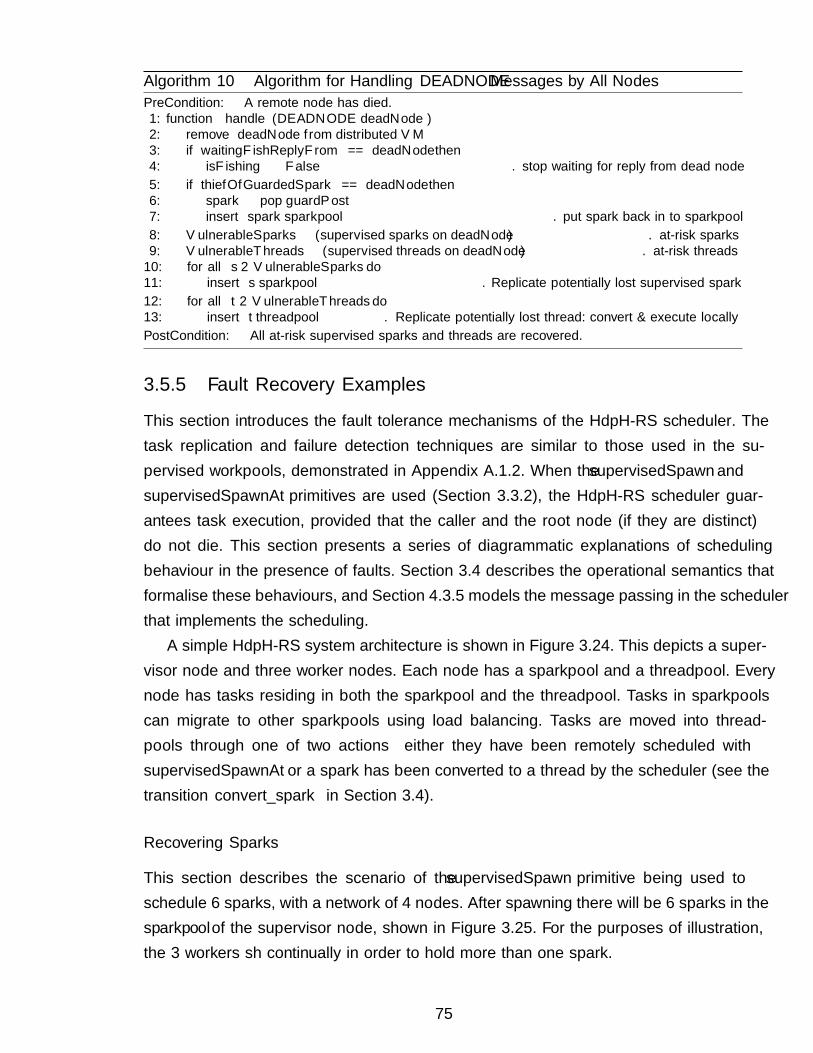
Algorithm 10 Algorithm for Handling DEADNODE Messages by All NodesPreCondition: A remote node has died.1: function handle(DEADNODE deadNode)2: remove deadNode from distributed VM3: if waitingF ishReplyFrom == deadNode then4: isF ishing ← False . stop waiting for reply from dead node5: if thiefOfGuardedSpark == deadNode then6: spark ← pop guardPost7: insert spark sparkpool . put spark back in to sparkpool8: V ulnerableSparks← (supervised sparks on deadNode) . at-risk sparks9: V ulnerableThreads← (supervised threads on deadNode) . at-risk threads10: for all s ∈ V ulnerableSparks do11: insert s sparkpool . Replicate potentially lost supervised spark12: for all t ∈ V ulnerableThreads do13: insert t threadpool . Replicate potentially lost thread: convert & execute locallyPostCondition: All at-risk supervised sparks and threads are recovered.

3.5.5 Fault Recovery Examples

This section introduces the fault tolerance mechanisms of the HdpH-RS scheduler. Thetask replication and failure detection techniques are similar to those used in the su-pervised workpools, demonstrated in Appendix A.1.2. When the supervisedSpawn andsupervisedSpawnAt primitives are used (Section 3.3.2), the HdpH-RS scheduler guar-antees task execution, provided that the caller and the root node (if they are distinct)do not die. This section presents a series of diagrammatic explanations of schedulingbehaviour in the presence of faults. Section 3.4 describes the operational semantics thatformalise these behaviours, and Section 4.3.5 models the message passing in the schedulerthat implements the scheduling.

A simple HdpH-RS system architecture is shown in Figure 3.24. This depicts a super-visor node and three worker nodes. Each node has a sparkpool and a threadpool. Everynode has tasks residing in both the sparkpool and the threadpool. Tasks in sparkpoolscan migrate to other sparkpools using load balancing. Tasks are moved into thread-pools through one of two actions — either they have been remotely scheduled withsupervisedSpawnAt or a spark has been converted to a thread by the scheduler (see thetransition convert_spark in Section 3.4).

Recovering Sparks

This section describes the scenario of the supervisedSpawn primitive being used toschedule 6 sparks, with a network of 4 nodes. After spawning there will be 6 sparks in thesparkpool of the supervisor node, shown in Figure 3.25. For the purposes of illustration,the 3 workers fish continually in order to hold more than one spark.

75

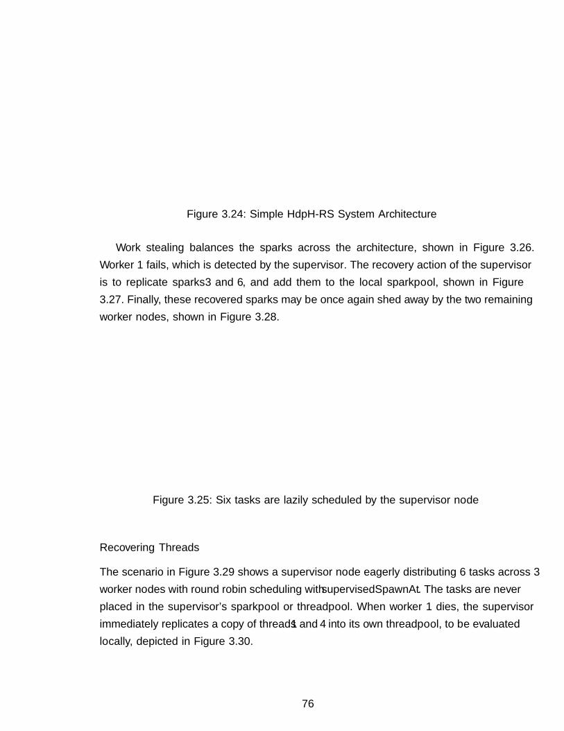
Supervisor

Worker 1

S S ST T T

TS

Worker 2 Worker 3

Figure 3.24: Simple HdpH-RS System Architecture

Work stealing balances the sparks across the architecture, shown in Figure 3.26.Worker 1 fails, which is detected by the supervisor. The recovery action of the supervisoris to replicate sparks 3 and 6, and add them to the local sparkpool, shown in Figure3.27. Finally, these recovered sparks may be once again fished away by the two remainingworker nodes, shown in Figure 3.28.

Supervisor

Worker 1

S S ST T T

TS

Worker 2 Worker 3

3

5 6

4

21

Figure 3.25: Six tasks are lazily scheduled by the supervisor node

Recovering Threads

The scenario in Figure 3.29 shows a supervisor node eagerly distributing 6 tasks across 3worker nodes with round robin scheduling with supervisedSpawnAt. The tasks are neverplaced in the supervisor’s sparkpool or threadpool. When worker 1 dies, the supervisorimmediately replicates a copy of threads 1 and 4 into its own threadpool, to be evaluatedlocally, depicted in Figure 3.30.

76

1

6 5 43 2

Supervisor

Worker 1

S S ST T T

TS

Worker 2 Worker 3

Figure 3.26: Six tasks are fished equally by 3 worker nodes

1

5 42

3

6

Supervisor

S ST T T

TS

Worker 2 Worker 3Worker 1

S

Figure 3.27: A worker node fails, and copies of lost tasks are rescheduled by the supervisor

Simultaneous Failure

There are failure scenarios whereby the connection between the root node and multipleother nodes may be lost. Communication links may fail by crashing, or by failing to delivermessages. Combinations of such failures may lead to partitioning failures [46], where nodesin a partition may continue to communicate with each other, but no communication canoccur between sites in different partitions.

There are two distinguished connected graphs in the distributed HdpH-RS virtualmachine. First is the networking hardware between hosts. Sockets over TCP/IP is usedon Ethernet networking infrastructures in HdpH-RS (Section 5.5) to send and receivemessages. The maximum size of this connected graph is fixed, hosts cannot be addedduring runtime.

The second graph connects tasks to futures. Recall from Section 3.3.2 that futuresare created with the spawn family of primitives. A task may be decomposed in to smallertasks, creating futures recursively.

77

1

5 42

6

3

Supervisor

S ST T T

TS

Worker 2 Worker 3Worker 1

S

Figure 3.28: The rescheduled tasks are once again fished away

1 2 3

Supervisor

Worker 1

S S ST T T

TS

Worker 2 Worker 3

4 5 6

Figure 3.29: Six tasks are eagerly scheduled as threads to 3 worker nodes

A simple graph expansion of futures is shown in Figure 3.31. All nodes in a dottedarea are connected in a network. Nodes A and B are connected. Node A takes the roleof the root node and starts the computation, which splits the program into 30 tasks.During runtime, 5 unevaluated tasks are stolen by node B over the network connection.These 5 tasks are expanded in to 10, so node B holds 10 tasks. The program in total hastherefore expanded to a graph of 35 futures. The key point is that in both the absenceand presence of faults, this program will always expand to 35 futures.

A slightly more complicated decomposition is in Figure 3.32. This program is ex-panded to a graph of 54 futures in total, over 5 nodes including the root node.

The failure scenario is shown in Figure 3.33. The network is split in to two partitions,one comprised of nodes A, B and C, and the other with nodes D and E. A lost partitionis one that no longer includes the root node A. The static network connection from theroot node A to both D and E are lost, and so D and E are zombie nodes. Despite the factthat the connection with the root node was lost by D and E simultaneously, notificationof connection loss from these nodes will arrive sequentially at A, B and C. Nodes D

78

2 3

1

4

Supervisor

S ST T

TS

Worker 2 Worker 3

5 6

Worker 1

TS

Figure 3.30: Copies of the two lost tasks are converted to threads on the supervisor node

BA1−>30 5−>105

Figure 3.31: Graph Expansion of Tasks

and E will receive notification that connection with root node A has been lost, and willterminate as they know they can no longer play a useful role in the execution of thecurrent job.

The recovery of tasks is shown in Figure 3.34. Nodes A, B and C check whether theselost connections affect the context of the futures they host locally. Node A concludes thatit is completely unaffected by the connection loss. Node B concludes that it is affectedby the loss of node D, and must recover 3 tasks. Node C concludes that it is affected bythe loss of node E, and must recover 8 tasks. These tasks will once again expand from 3to 6, and 8 to 14, respectively.

The scenario in this section demonstrates that in the presence of network failure,incurring the loss of connection from the root node to two nodes, the program executingon the partition containing the root node expands to 54 futures — the same as failure-freeevaluation.

5−>10 3−>6

8−>14

20

1−>30 A

C E

DB5

8

3

20−>30

Figure 3.32: Graph Expansion of Tasks over 5 Nodes

79

5−>10 3−>6

8−>14

20

1−>30 A

C E

DB5

20−>30

Figure 3.33: Network Partition, Leaving Nodes D & E Isolated

A

C E

DB

20−>30

5−>10 3−>6

8−>14

1−>30

*3−>6

*8−>14

Figure 3.34: Recovering Tasks from Nodes D & E

3.6 Summary

This chapter has presented the language and scheduling design of a HdpH-RS. The nextchapter presents a Promela model of the scheduling algorithm from Section 3.5.4. A keyproperty is verified using the SPIN model checker. This property states that a supervisedfuture (Section 3.3.1) is eventually filled despite all possible combinations of node fail-ure. Chapter 5 then presents a Haskell implementation of the HdpH-RS programmingprimitives and the verified reliable scheduling design.

80

Chapter 4

The Validation of ReliableDistributed Scheduling for HdpH-RS

Chapter 3 presents the design of HdpH-RS — the fault tolerant programming primitivessupervisedSpawn and supervisedSpawnAt (Section 3.3.2) supported by a reliable sched-uler (Section 3.5). This chapter validates the critical reliable properties of the scheduler.The SPIN model checker is used to ensure that the HdpH-RS scheduling algorithms (Sec-tion 3.5.4) honour the small-step semantics on states (Section 3.4), supervising sparks inthe absence and presence of faults.

Model checking has been shown to be an effective tool in validating the behaviourof fault tolerant systems, such as embedded spacecraft controllers [143], reliable broad-casting algorithms [91], and fault tolerant real-time startup protocols for safety criticalapplications [57]. Model checking has previously been used to eliminate non-progresscycles of process scheduling in asynchronous distributed systems [83].

Fault tolerant distributed algorithms are central to building reliable distributed sys-tems. Due to the various sources of non-determinism in faulty systems, it is easy to makemistakes in the correctness arguments for fault tolerant distributed systems. They aretherefore natural candidates for model checking [91]. The HdpH-RS scheduler must holdreliability properties when scaled to complex non-deterministic distributed environments:

1. Asynchronous message passing Causal ordering [99] of asynchronous dis-tributed scheduling events is not consistent with wall-clock times. Message passingbetween nodes is asynchronous and non-blocking, instead writing to channel buffers.Because of communication delays, the information maintained in a node concerningits neighbours’ workload could be outdated [186].

2. Work stealing Idle nodes attempt to steal work from overloaded nodes. To recovertasks in the presence of failure, a supervisor must be able to detect node failure and

81

must always know the location of its supervised tasks. The asynchronous messagepassing from (1) complicates location tracking. The protocol for reliably relocatingsupervised tasks between nodes in the presence of failure is intricate, and modelchecking the protocol increases confidence in the design.

3. Node failure Failure is commonly detected with timeouts or ping-pong protocols(Section 2.2.3). The Promela abstraction models node failure, and latency’s of nodefailure detection.

The model of the HdpH-RS scheduler shows that by judiciously abstracting away ex-traneous complexity of the HdpH-RS implementation, the state space can be exhaustivelysearched for validating a key reliability requirement. The key HdpH-RS reliable schedul-ing property is validated with SPIN [83] [84] in Section 4.4, by defining a correspondingsafety property in linear temporal logic. Bugs were fixed in earlier versions of the Promelamodel, when violating system states were identified. An example of bug finding using thisiterative implementation of HdpH-RS using model checking is described in Section 4.6.

The motivation for modeling work stealing in asynchronous environments is given inSection 4.1. The scope of the Promela abstraction of the HdpH-RS scheduler is in Section4.2. The model of the work stealing scheduler is in Section 4.3. The use of linear temporallogic for expression a key reliability property is shown in Section 4.4. The SPIN modelchecker to exhaustively search the model’s state space to validate that the reliabilityproperty holds on all reachable states. The SPIN model checking results are in Section4.5.

4.1 Modeling Asynchronous Environments

4.1.1 Asynchronous Message Passing

Most message passing technologies in distributed systems can be categorised in to threeclasses [168]: unreliable datagrams, remote procedure calls and reliable data streams. Un-reliable datagrams discard corrupt messages, but do little additional processing. Messagesmay be lost, duplicated or delivered out of order. An example is UDP [131]. In remoteprocedure calls, communication is presented as a procedure invocation that returns aresult. When failure does occur however, the sender is unable to distinguish whetherthe destination failed before or after receiving the request, or whether the network hasdelayed the reply. Reliable data streams communicate over channels that provide flowcontrol and reliable, sequenced message delivery. An example is TCP [133].

82

A TCP connection in the absence of faults provides FIFO ordering between two nodes.The relationship between messaging events can be described as causal ordering. Causalordering is always consistent with the actual wall-clock times that events occur. Thiscan be written as send(m1) → send(m2) [99], where → means happened-before. Theordering property of TCP guarantees that recv(m1) occurs before recv(m2) on the otherend of the connection. This ordering guarantee is not sufficient in distributed systemsthat have multiple TCP connections. The latency of TCP data transfer is well known [29],for example due to memory copying with kernel buffers, heterogeneous network latency,and TCP data transfer latency [29].

HdpH-RS uses a network abstraction layer [44] that assigns an endpoint to each node.An endpoint is a mailbox that consumes messages from multiple connections establishedwith other nodes. Causal ordering of messaging events is no longer consistent with wall-clock time. This potentially leads to overtaking on two separate TCP connections.

Take a simple architecture with three nodes A, B and C. If A is connected with Bon dual connection c1 and to C on dual connection c2, then the endpoint EA on nodeA is defined as EA = {c1, c2}. Nodes B and C send messages to EA in the causal orderc1.send(m1) → c2.send(m2). Ordering of events c1.recv(m1) and c2.recv(m2) at EA isunknown. The HdpH-RS work stealing protocol enforces a certain order of events, andmessage responses are determined by task location state (Section 3.5.4).

4.1.2 Asynchronous Work Stealing

Work stealing for balancing load is introduced in Section 3.2, describing how nodes inheritthief, victim and supervisory roles dynamically. Location tracker messages sent by a thiefand a victim with respect to a spark migrating between the two may be received in anyorder by the spark’s supervisor due to asynchronous message passing (Section 4.1.1).

The HdpH-RS fishing protocol gives the control of spark migration to the supervi-sor. The fishing protocol (Section 3.5.1) is abstracted in Promela in Section 4.2. Theprotocol handles any message sequence from thieves and victims to ensure that tasklocation tracking is never invalidated. The Promela model honours the small-step transi-tion rules migrate_supervised_spark and recover_supervised_spark (Section 3.4.3)for migrating and replicating supervised sparks shown in Section 4.3.3. The kill_node

transition rule in the small-step semantics can be triggered at any time as described inSection 4.3.2. This is modelled in Promela with a non-deterministic unconditional choicethat workers can take (Section 4.3.1).

83

4.2 Promela Model of Fault Tolerant Scheduling

4.2.1 Introduction to Promela

Promela is a meta-language for building verification models, and the language featuresare intended to facilitate the construction of high-level abstractions of distributed sys-tems. It is not a systems implementation language. The emphasis in Promela abstrac-tion is synchronisation and coordination with messages, rather than computation. Itsupports for example, the specification of non-deterministic control structures and it in-cludes primitives for process creation, and a fairly rich set of primitives for interprocesscommunication. Promela is not a programming language [84], and so does not supportfunctions that returns values and function pointers. This chapter verifies the fault tol-erant scheduler from Section 3.5. Chapter 5 presents the Haskell implementation of theverified scheduler and HdpH-RS programming primitives. The SPIN analyser is used toverify fractions of process behaviour, that are considered suspect [89].

Temporal logic model checking is a method for automatically deciding if a finite stateprogram satisfies its specification [37]. Since the size of the state space grows exponen-tially with the number of processes, model checking techniques based on explicit stateenumeration can only handle relatively small examples [36]. When the number of statesis large, it may be very difficult to determine is such a program is correct. Hence, theinfinite state space of the real HdpH-RS scheduler is abstracted to be a small finite modelthat SPIN can verify.

The HdpH-RS scheduler has been simplified to its core supervision behaviours thatensure supervised task survival. The model includes 1 supervisor, 3 workers and 1 su-pervised spark. The abstract model is sufficiently detailed to identify real bugs in theimplementation e.g. the identified bug described in Section 4.6.

SPIN is not a simulation or an application environment, it is a formal verifica-tion environment. Is this really a model that will comply with the correctnessrequirements only if the number of channels is 1,000? If so, I would considerthat a design error in itself. Gerard J. Holzmann [90]

Constructing Promela Models

Promela programs consist of processes, message channels, and variables. Processes areglobal objects that represent the concurrent nodes in HdpH-RS. Message channels forthe supervisor and workers are declared globally. The variables used in the propositionalsymbols in LTL formulae (Section 4.4) are declared globally. Other variables are declared

84

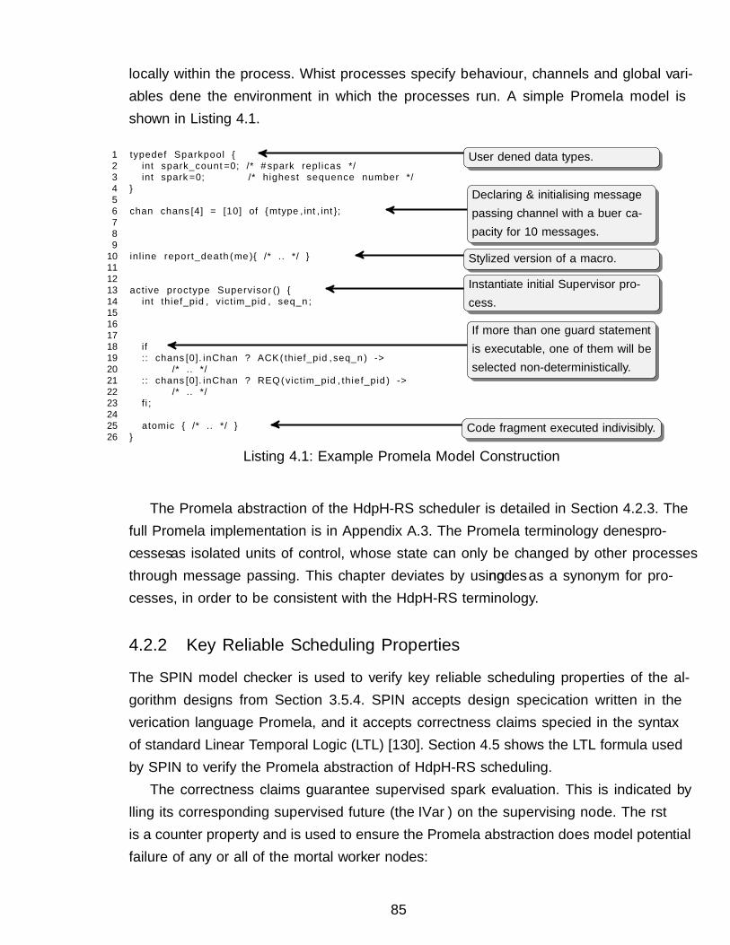
locally within the process. Whist processes specify behaviour, channels and global vari-ables define the environment in which the processes run. A simple Promela model isshown in Listing 4.1.

1 typedef Sparkpool {2 int spark_count =0; /* # spark replicas */3 int spark =0; /* highest sequence number */4 }56 chan chans [4] = [10] of {mtype ,int ,int };789

10 inline report_death (me ){ /* .. */ }111213 active proctype Supervisor () {14 int thief_pid , victim_pid , seq_n ;15161718 if19 :: chans [0]. inChan ? ACK(thief_pid , seq_n ) ->20 /* .. */21 :: chans [0]. inChan ? REQ( victim_pid , thief_pid ) ->22 /* .. */23 fi;2425 atomic { /* .. */ }26 }

Listing 4.1: Example Promela Model Construction

The Promela abstraction of the HdpH-RS scheduler is detailed in Section 4.2.3. Thefull Promela implementation is in Appendix A.3. The Promela terminology defines pro-cesses as isolated units of control, whose state can only be changed by other processesthrough message passing. This chapter deviates by using nodes as a synonym for pro-cesses, in order to be consistent with the HdpH-RS terminology.

4.2.2 Key Reliable Scheduling Properties

The SPIN model checker is used to verify key reliable scheduling properties of the al-gorithm designs from Section 3.5.4. SPIN accepts design specification written in theverification language Promela, and it accepts correctness claims specified in the syntaxof standard Linear Temporal Logic (LTL) [130]. Section 4.5 shows the LTL formula usedby SPIN to verify the Promela abstraction of HdpH-RS scheduling.

The correctness claims guarantee supervised spark evaluation. This is indicated byfilling its corresponding supervised future (the IVar) on the supervising node. The firstis a counter property and is used to ensure the Promela abstraction does model potentialfailure of any or all of the mortal worker nodes:

85

User defined data types.

Declaring & initialising messagepassing channel with a buffer ca-pacity for 10 messages.

Stylized version of a macro.

Instantiate initial Supervisor pro-cess.

If more than one guard statementis executable, one of them will beselected non-deterministically.

Code fragment executed indivisibly.

1. Any or all worker nodes may fail To check that the model potentially kills oneor more mortal workers, SPIN is used to find counter-example executions when oneof the workers terminates, which it is trivially able to do after searching 5 uniquestates (Section 4.5.1).

Two further properties are used to exhaustively verify the absence of non-desirablestates of the IVar on the supervisor node:

1. The IVar is empty until a result is sent Evaluating a task involves transmittinga value to the supervisor, the host of the IVar. This property verifies that the IVarcannot be full until one of the nodes has transmitted a value to the supervisor.The absence of a counter system state is verified after exhaustively searching 3.66million states (Section 4.5.2).

2. The IVar is eventually always full The IVar will eventually be filled by either aremaining worker, or the supervisor. This is despite the failure of any or all workernodes. Once it is full, it will always be full because there are no operations to removevalues from IVars in HdpH-RS. The absence of a counter system state is verifiedafter exhaustively searching 8.22 million states (Section 4.5.2).

4.2.3 HdpH-RS Abstraction

The model considers tasks scheduled with supervisedSpawn in HdpH-RS — modelingthe tracking and recovery of supervised sparks. The location of threads scheduled withsupervisedSpawnAt is always known i.e. the scheduling target. This would not elicitrace conditions on location tracking messages REQ and ACK, and are therefore not inthe scope of the model. The Promela model is a partial abstraction that encapsulatesbehaviours necessary for guaranteeing the evaluation of supervised sparks. There are sixcharacteristics of the HdpH-RS scheduler in the Promela model:

1. One immortal supervisor that initially puts a spark into its local sparkpool. Italso creates spark replicas when necessary (item 6).

2. Three mortal workers that attempt to steal work from the supervisor and eachother. Failure of these nodes is modeled by terminating the Promela process foreach node.

3. Computation of a spark may happen at any time by any node that holds a copyof the spark. This simulates the execution of the spark, which would invoke an rput

call to fill the IVar on the supervisor. It is modeled by sending a RESULT message to

86

the supervisor. This message type is not in HdpH-RS, rather it mimics PUSH usedby rput to transmit a value to an IVar in HdpH-RS.

4. Failure of a worker node means that future messages to it are lost. The kill_nodetransition rule is modeled with a non-deterministic suicidal choice any of the threeworker nodes can make. This choice results in a node asynchronously broadcastingits death to the remaining healthy nodes and then terminating. Failure detectionis modeled by healthy nodes receiving DEADNODE messages.

5. Asynchronicity of both message passing and failure detection is modeled inPromela using buffered channels. Buffered channels model the buffered FIFO TCPconnections in HdpH-RS.

6. Replication is used by the supervisor to ensure the safety of a potentially lostspark in the presence of node failure. The model includes spark replication from al-gorithm 10 in Section 3.5.4, honouring the recover_supervised_spark small-steptransition rule in Section 3.4.3. Replication numbers are used to tag spark replicasin order to identify obsolete spark copies. Obsolete replica migration could poten-tially invalidate location records for a supervised spark, described in Section 3.5.3.Therefore, victims are asked to discard obsolete sparks, described in Algorithm 5of Section 3.5.4.

Two scheduling properties in Section 4.4.1 state that a property must eventually betrue. The formula � (ivar_empty U any_result_sent) in Section 4.4.1 is a strong untilconnective and verifies two properties of the model. First, that the ivar_empty propertymust hold until at least any_result_sent is true. Second, that any_result_sent is truein some future state (the weak until connective does not demand this second property).The formula ♦ � ivar_full demands that the IVar on the supervisor is eventually alwaysfull.

Without any deterministic choice of sending a RESULT message to the supervisor, thethree thieving worker nodes could cycle through a sequence of work stealing messages,forever passing around the spark and each time visiting an identical system state. TheSPIN model checker identified this cyclic trace in an earlier version of the model. Thesecycles contradict the temporal requirements of the strong until and eventually connectivesin the two properties above.

Determinism is introduced to the model by ageing the spark through transitions of themodel. The age of the spark is zero at the initial system state. Each time it is scheduledto a node, its age is incremented. Moreover, each time it must be replicated by the

87

supervisor its age is again incremented. When the age of the spark reaches 100, all nodesare forced to make a deterministic choice to send a RESULT message to the supervisor ifthey hold a replica or else the next time they do. This models the HdpH-RS assumptionthat a scheduler will eventually execute the spark in a sparkpool.

4.2.4 Out-of-Scope Characteristics

Some aspects of the HdpH-RS scheduler design and implementation are not abstractedin to the Promela model, because they are not part of the fault tolerance actions toguarantee that an IVar will be written to.

1. Multiple IVars The model involves only one IVar and one supervised spark, whichmay manifest into multiple replicas — one active and the rest obsolete. MultipleIVars are not modeled.

2. Non-supervised sparks Only supervised sparks created with supervisedSpawn

are modeled, while unsupervised sparks are not. Non-supervised sparks are cre-ated by calls to spawn (Section 3.3.2), and create sparks that are intentionally notresilient to faults, and by-pass the fault tolerant fishing protocol.

3. Threads Threads are created with spawnAt and supervisedSpawnAt. Section 3.3.2describes why eagerly placed threads are more straight forward to supervise. Oncethey are transmitted to a target node, they do not migrate.

4.3 Scheduling Model

4.3.1 Channels & Nodes

Nodes interact with message passing. Using Promela syntax, nodes receive messages with?, and send messages with !. A simple example is shown in Figure 4.1. Node A sends amessage FOO with ! to a channel that node B receives messages on. Node B reads themessage from the channel with ?. The channels in the Promela model of HdpH-RS areasynchronous, so that messages can be sent to a channel buffer, rather than being blockedwaiting on a synchronised participatory receiver. This reflects the data buffers in TCPsockets, the transport protocol in HdpH-RS.

Channels

There are four channels in the model, one for each of the four nodes. They are globallydefined as shown on line 1 of Listing 4.2. The channels can store up to ten messages, which

88

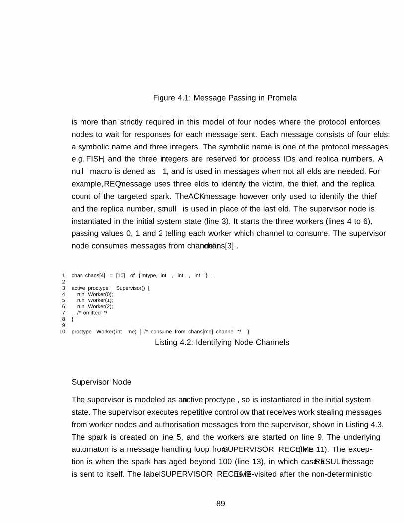
Node Asender

Node Breceiver

B ! FOOFOO

B ? FOO

Figure 4.1: Message Passing in Promela

is more than strictly required in this model of four nodes where the protocol enforcesnodes to wait for responses for each message sent. Each message consists of four fields:a symbolic name and three integers. The symbolic name is one of the protocol messagese.g. FISH, and the three integers are reserved for process IDs and replica numbers. Anull macro is defined as −1, and is used in messages when not all fields are needed. Forexample, REQ message uses three fields to identify the victim, the thief, and the replicacount of the targeted spark. The ACK message however only used to identify the thiefand the replica number, so null is used in place of the last field. The supervisor node isinstantiated in the initial system state (line 3). It starts the three workers (lines 4 to 6),passing values 0, 1 and 2 telling each worker which channel to consume. The supervisornode consumes messages from channel chans[3].

1 chan chans[4] = [10] of {mtype, int , int , int } ;23 active proctype Supervisor() {4 run Worker(0);5 run Worker(1);6 run Worker(2);7 /* omitted */8 }9

10 proctype Worker(int me) { /* consume from chans[me] channel */ }

Listing 4.2: Identifying Node Channels

Supervisor Node

The supervisor is modeled as an active proctype, so is instantiated in the initial systemstate. The supervisor executes repetitive control flow that receives work stealing messagesfrom worker nodes and authorisation messages from the supervisor, shown in Listing 4.3.The spark is created on line 5, and the workers are started on line 9. The underlyingautomaton is a message handling loop from SUPERVISOR_RECEIVE (line 11). The excep-tion is when the spark has aged beyond 100 (line 13), in which case a RESULT messageis sent to itself. The label SUPERVISOR_RECEIVE is re-visited after the non-deterministic

89

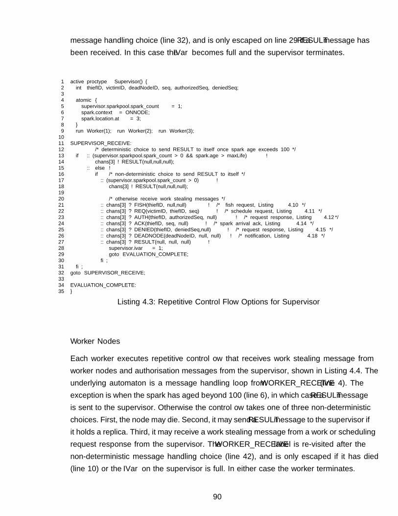
message handling choice (line 32), and is only escaped on line 29 if a RESULT message hasbeen received. In this case the IVar becomes full and the supervisor terminates.

1 active proctype Supervisor() {2 int thiefID, victimID, deadNodeID, seq, authorizedSeq, deniedSeq;34 atomic {5 supervisor.sparkpool.spark_count = 1;6 spark.context = ONNODE;7 spark.location.at = 3;8 }9 run Worker(1); run Worker(2); run Worker(3);

1011 SUPERVISOR_RECEIVE:12 /* deterministic choice to send RESULT to itself once spark age exceeds 100 */13 if :: (supervisor.sparkpool.spark_count > 0 && spark.age > maxLife) →14 chans[3] ! RESULT(null,null,null);15 :: else →16 if /* non-deterministic choice to send RESULT to itself */17 :: (supervisor.sparkpool.spark_count > 0) →18 chans[3] ! RESULT(null,null,null);1920 /* otherwise receive work stealing messages */21 :: chans[3] ? FISH(thiefID, null,null) → /* fish request, Listing 4.10 */22 :: chans[3] ? REQ(victimID, thiefID, seq) → /* schedule request, Listing 4.11 */23 :: chans[3] ? AUTH(thiefID, authorizedSeq, null) → /* request response, Listing 4.12*/24 :: chans[3] ? ACK(thiefID, seq, null) → /* spark arrival ack, Listing 4.14 */25 :: chans[3] ? DENIED(thiefID, deniedSeq,null) → /* request response, Listing 4.15 */26 :: chans[3] ? DEADNODE(deadNodeID, null, null) → /* notification, Listing 4.18 */27 :: chans[3] ? RESULT(null, null, null) →28 supervisor.ivar = 1;29 goto EVALUATION_COMPLETE;30 fi;31 fi;32 goto SUPERVISOR_RECEIVE;3334 EVALUATION_COMPLETE:35 }

Listing 4.3: Repetitive Control Flow Options for Supervisor

Worker Nodes

Each worker executes repetitive control flow that receives work stealing message fromworker nodes and authorisation messages from the supervisor, shown in Listing 4.4. Theunderlying automaton is a message handling loop from WORKER_RECEIVE (line 4). Theexception is when the spark has aged beyond 100 (line 6), in which case a RESULT messageis sent to the supervisor. Otherwise the control flow takes one of three non-deterministicchoices. First, the node may die. Second, it may send a RESULTmessage to the supervisor ifit holds a replica. Third, it may receive a work stealing message from a work or schedulingrequest response from the supervisor. The WORKER_RECEIVE label is re-visited after thenon-deterministic message handling choice (line 42), and is only escaped if it has died(line 10) or the IVar on the supervisor is full. In either case the worker terminates.

90

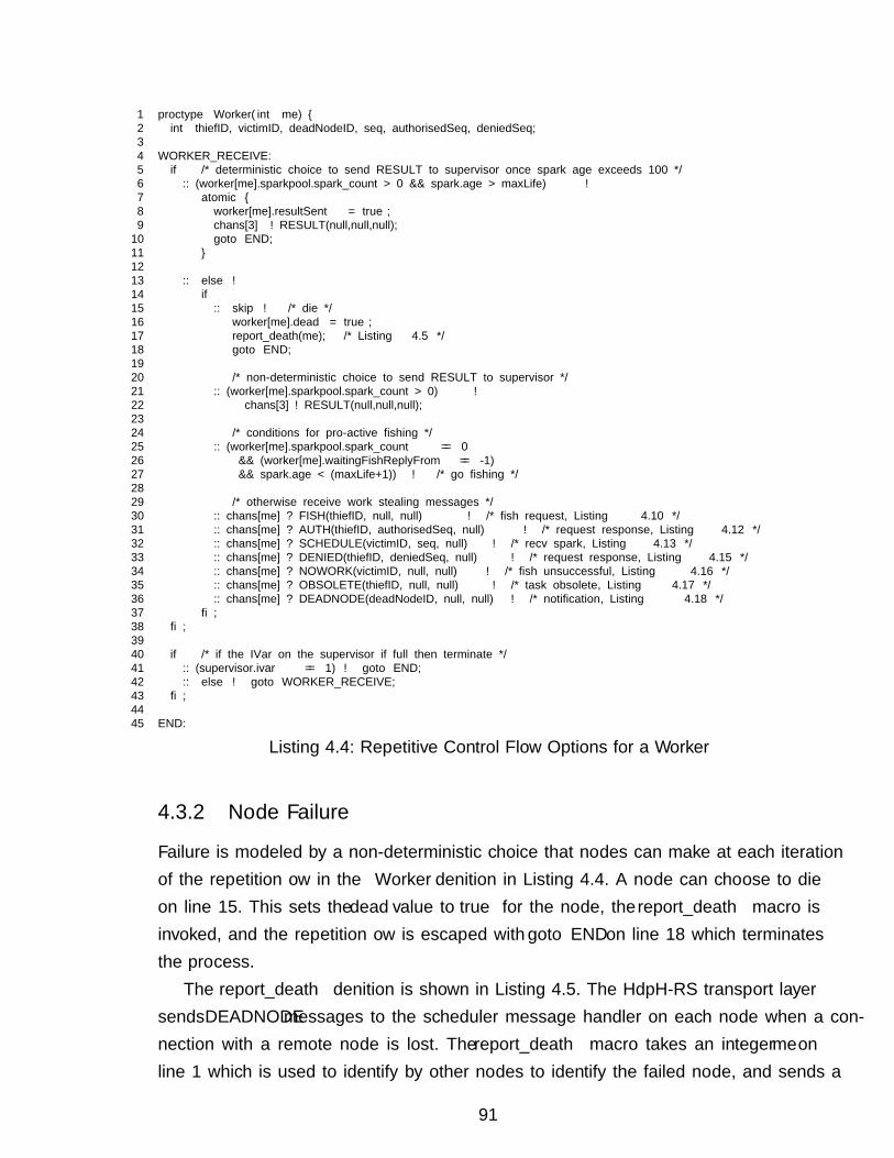
1 proctype Worker(int me) {2 int thiefID, victimID, deadNodeID, seq, authorisedSeq, deniedSeq;34 WORKER_RECEIVE:5 if /* deterministic choice to send RESULT to supervisor once spark age exceeds 100 */6 :: (worker[me].sparkpool.spark_count > 0 && spark.age > maxLife) →7 atomic {8 worker[me].resultSent = true;9 chans[3] ! RESULT(null,null,null);

10 goto END;11 }1213 :: else →14 if15 :: skip → /* die */16 worker[me].dead = true;17 report_death(me); /* Listing 4.5 */18 goto END;1920 /* non-deterministic choice to send RESULT to supervisor */21 :: (worker[me].sparkpool.spark_count > 0) →22 chans[3] ! RESULT(null,null,null);2324 /* conditions for pro-active fishing */25 :: (worker[me].sparkpool.spark_count == 026 && (worker[me].waitingFishReplyFrom == -1)27 && spark.age < (maxLife+1)) → /* go fishing */2829 /* otherwise receive work stealing messages */30 :: chans[me] ? FISH(thiefID, null, null) → /* fish request, Listing 4.10 */31 :: chans[me] ? AUTH(thiefID, authorisedSeq, null) → /* request response, Listing 4.12 */32 :: chans[me] ? SCHEDULE(victimID, seq, null) → /* recv spark, Listing 4.13 */33 :: chans[me] ? DENIED(thiefID, deniedSeq, null) → /* request response, Listing 4.15 */34 :: chans[me] ? NOWORK(victimID, null, null) → /* fish unsuccessful, Listing 4.16 */35 :: chans[me] ? OBSOLETE(thiefID, null, null) → /* task obsolete, Listing 4.17 */36 :: chans[me] ? DEADNODE(deadNodeID, null, null) → /* notification, Listing 4.18 */37 fi;38 fi;3940 if /* if the IVar on the supervisor if full then terminate */41 :: (supervisor.ivar == 1) → goto END;42 :: else → goto WORKER_RECEIVE;43 fi;4445 END:

Listing 4.4: Repetitive Control Flow Options for a Worker

4.3.2 Node Failure

Failure is modeled by a non-deterministic choice that nodes can make at each iterationof the repetition flow in the Worker definition in Listing 4.4. A node can choose to dieon line 15. This sets the dead value to true for the node, the report_death macro isinvoked, and the repetition flow is escaped with goto END on line 18 which terminatesthe process.

The report_death definition is shown in Listing 4.5. The HdpH-RS transport layersends DEADNODE messages to the scheduler message handler on each node when a con-nection with a remote node is lost. The report_death macro takes an integer me online 1 which is used to identify by other nodes to identify the failed node, and sends a

91

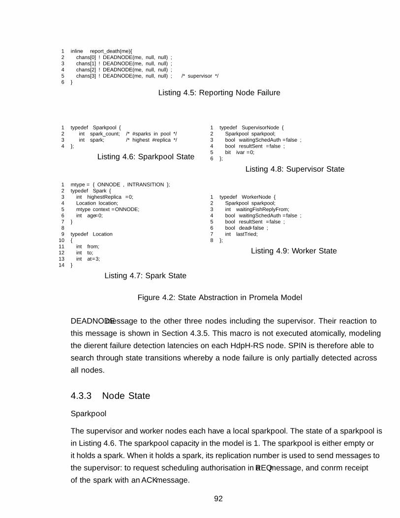
1 inline report_death(me){2 chans[0] ! DEADNODE(me, null, null) ;3 chans[1] ! DEADNODE(me, null, null) ;4 chans[2] ! DEADNODE(me, null, null) ;5 chans[3] ! DEADNODE(me, null, null) ; /* supervisor */6 }

Listing 4.5: Reporting Node Failure

1 typedef Sparkpool {2 int spark_count; /* #sparks in pool */3 int spark; /* highest #replica */4 };

Listing 4.6: Sparkpool State

1 mtype = { ONNODE , INTRANSITION };2 typedef Spark {3 int highestReplica=0;4 Location location;5 mtype context=ONNODE;6 int age=0;7 }89 typedef Location

10 {11 int from;12 int to;13 int at=3;14 }

Listing 4.7: Spark State

1 typedef SupervisorNode {2 Sparkpool sparkpool;3 bool waitingSchedAuth=false;4 bool resultSent=false;5 bit ivar=0;6 };

Listing 4.8: Supervisor State

1 typedef WorkerNode {2 Sparkpool sparkpool;3 int waitingFishReplyFrom;4 bool waitingSchedAuth=false;5 bool resultSent=false;6 bool dead=false;7 int lastTried;8 };

Listing 4.9: Worker State

Figure 4.2: State Abstraction in Promela Model

DEADNODE message to the other three nodes including the supervisor. Their reaction tothis message is shown in Section 4.3.5. This macro is not executed atomically, modelingthe different failure detection latencies on each HdpH-RS node. SPIN is therefore able tosearch through state transitions whereby a node failure is only partially detected acrossall nodes.

4.3.3 Node State

Sparkpool

The supervisor and worker nodes each have a local sparkpool. The state of a sparkpool isin Listing 4.6. The sparkpool capacity in the model is 1. The sparkpool is either empty orit holds a spark. When it holds a spark, its replication number is used to send messages tothe supervisor: to request scheduling authorisation in a REQ message, and confirm receiptof the spark with an ACK message.

92

The spark’s Location is stored in location and context on lines 4 and 5 of Listing4.7, which are modified by the supervisor when REQ and ACK messages are received. Thelocation context of the supervised spark is either ONNODE or INTRANSITION (Section 3.5.2).The most recently allocated replica number is held in highestReplica on line 3, and isinitially set to 0. The age of the spark on line 6 is initially set to 0, and is incrementedwhen the spark is scheduled to another node or when it is replicated.

The actual expression in the spark is not modeled. The indistinguishable scenariowhen an IVar is written either once or multiple times is demonstrated with executionsthrough the operational semantics in Section 3.4.4. Any node, including the supervisor,may transmit a result to the supervisor if it holds a spark copy. As such, a spark is simplyrepresented as its replication count (line 3).

Supervisor State

The local state of the supervisor is shown in Listing 4.8. In the initial system state, itadds the spark to its sparkpool (line 2), which may be fished away by a worker node. Tominimise the size of the state machine, the supervisor does not try to steal the spark orsubsequent replicas once they are fished away. The IVar is represented by a bit on line 5,0 for empty and 1 for full. Lastly, a waitingSchedAuth (line 3) is used to reject incomingREQ messages, whilst it waits for an AUTH from itself if it is targeted by a thief.

An example of modifying location tracking with the migrate_supervised_spark rule(Section 3.4.3) is shown in Figure 4.3. It is a more detailed version of the fault tolerantfishing protocol from Figure 3.16 of Section 3.5.2. The Promela message passing syntaxin the MSC is an abstraction of send and receive Haskell function calls in the HdpH-RS implementation (Section 5.5.2). Node B is the victim, and node C is the thief. NodeA hosts supervised future i{j〈〈M〉〉SB}A (Section 3.4.3). Once the message sequence iscomplete, the new supervised future state is i{j〈〈M〉〉SC}A.

An example of recovering a supervised spark with the recovery_supervised_sparkrule is shown in Figure 4.4. The supervised spark j of supervised future i{j〈〈M〉〉SC}A ison node C. The node hosting i receives a DEADNODE message about node C, and createsa new replica k. The existence and location state of k is added to the supervised futurei{k〈〈M〉〉SA}A.

Worker State

The local state of a worker is shown in Listing 4.9. When a thieving node proactively sendsa fish to another node, the waitingFishReplyFrom stores the channel index identifierfor the victim i.e. 0, 1 or 2 if targeting a worker node, or 3 if targeting the supervisor.

93

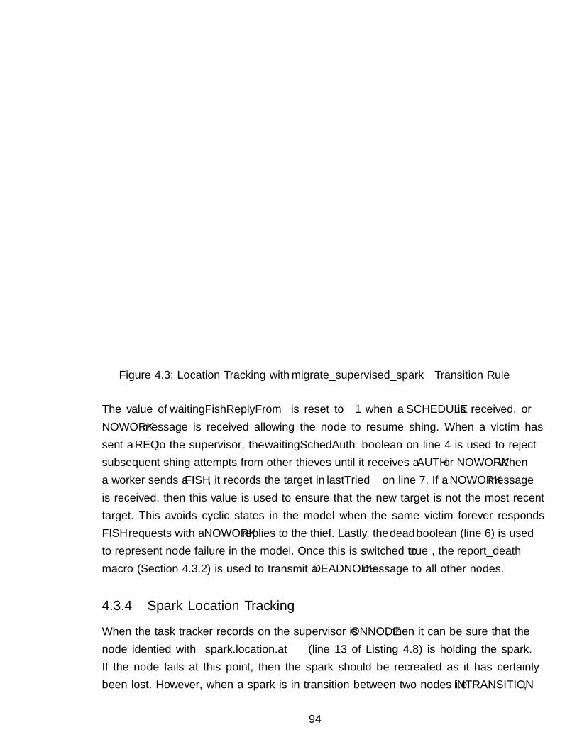
Node Asupervisor

Node Bvictim

Node Cthief

holds ..jB ! FISH C

OnNode B FISH C

B ? FISH C

A ! REQ i r0 B C

REQ i r0 B C

A ? REQ i r0 B C

B ! AUTH i C

AUTH i C

InTransition B C B ? AUTH i C

C ! SCHEDULE ..j B

SCHEDULE ..j B

C ? SCHEDULE ..j B

A ! ACK i r0ACK i r0

A ? ACK i r0

OnNode C

i{j⟪M⟫SB}A

i{j⟪M⟫SC}A

Figure 4.3: Location Tracking with migrate_supervised_spark Transition Rule

The value of waitingFishReplyFrom is reset to −1 when a SCHEDULE is received, orNOWORK message is received allowing the node to resume fishing. When a victim hassent a REQ to the supervisor, the waitingSchedAuth boolean on line 4 is used to rejectsubsequent fishing attempts from other thieves until it receives a AUTH or NOWORK. Whena worker sends a FISH, it records the target in lastTried on line 7. If a NOWORK messageis received, then this value is used to ensure that the new target is not the most recenttarget. This avoids cyclic states in the model when the same victim forever respondsFISH requests with a NOWORK replies to the thief. Lastly, the dead boolean (line 6) is usedto represent node failure in the model. Once this is switched to true, the report_deathmacro (Section 4.3.2) is used to transmit a DEADNODE message to all other nodes.

4.3.4 Spark Location Tracking

When the task tracker records on the supervisor is ONNODE, then it can be sure that thenode identified with spark.location.at (line 13 of Listing 4.8) is holding the spark.If the node fails at this point, then the spark should be recreated as it has certainlybeen lost. However, when a spark is in transition between two nodes i.e INTRANSITION,

94

Node Asupervisor

Node Bvictim

Node Cthief

holds ..jOnNode C

A ! DEADNODE C

DEADNODE CA ? DEADNODE C

holds ..k

OnNode A

i{j⟪M⟫SC}A

i{k⟪M⟫SA}A

Figure 4.4: Supervised Spark Recovery with recover_supervised_spark Transition Rule

the supervisor cannot be sure of the location of the spark (Section 3.5.2); it is on eitherof the nodes identified by spark.location.from or spark.location.to (lines 11 and12). To overcome this uncertainty, the model faithfully reflects the HdpH-RS pessimisticduplication strategy in algorithm 10 when a DEADNODE is received. This potentially gen-erates replicas that concurrently exist in the model. This is handled using replica counts(Section 3.5.3).

4.3.5 Message Handling

This section presents the message handling in the Promela abstraction that models thefault tolerant scheduling algorithm from Section 3.5.4. An example control flow sequenceon the supervisor is:

1. Receive a REQ from a victim targeted by a thief for supervised spark1.

2. Check that the location for spark1 is ONNODE victim.

3. Modify location status for spark1 to INTRANSITION victim thief.

4. Send an AUTH to the victim.

Steps 2 and 3 are indivisibly atomic in the HdpH-RS design, as the message handleron each node is single threaded. That is, steps 2, 3 and 4 are executed by the messagehandler before the next message is received. Location state is implemented in HdpH-RS as a mutable IORef variable, and steps 2 and 3 check and modify the state of theIORef atomically using atomicModifyIORef. The message handling in the Promela modeltherefore follows the pattern of: receiving a message; atomically modify local state; andpossibly ended with sending a message.

95

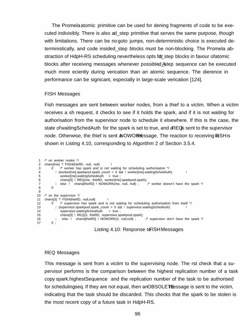
The Promela atomic primitive can be used for defining fragments of code to be exe-cuted indivisibly. There is also a d_step primitive that serves the same purpose, thoughwith limitations. There can be no goto jumps, non-deterministic choice is executed de-terministically, and code inside d_step blocks must be non-blocking. The Promela ab-straction of HdpH-RS scheduling nevertheless opts for d_step blocks in favour of atomicblocks after receiving messages whenever possible. A d_step sequence can be executedmuch more efficiently during verification than an atomic sequence. The difference inperformance can be significant, especially in large-scale verification [124].

FISH Messages

Fish messages are sent between worker nodes, from a thief to a victim. When a victimreceives a fish request, it checks to see if it holds the spark, and if it is not waiting forauthorisation from the supervisor node to schedule it elsewhere. If this is the case, thestate of waitingSchedAuth for the spark is set to true, and a REQ is sent to the supervisornode. Otherwise, the thief is sent a NOWORK message. The reaction to receiving a FISH isshown in Listing 4.10, corresponding to Algorithm 2 of Section 3.5.4.

1 /* on worker nodes */2 chans[me] ? FISH(thiefID, null, null) →3 if /* worker has spark and is not waiting for scheduling authorisation */4 :: (worker[me].sparkpool.spark_count > 0 && ! worker[me].waitingSchedAuth) →5 worker[me].waitingSchedAuth = true;6 chans[3] ! REQ(me, thiefID, worker[me].sparkpool.spark);7 :: else → chans[thiefID] ! NOWORK(me, null, null) ; /* worker doesn’t have the spark */8 fi9

10 /* on the supervisor */11 chans[3] ? FISH(thiefID, null,null) →12 if /* supervisor has spark and is not waiting for scheduling authorisation from itself */13 :: (supervisor.sparkpool.spark_count > 0 && ! supervisor.waitingSchedAuth) →14 supervisor.waitingSchedAuth = true;15 chans[3] ! REQ(3, thiefID, supervisor.sparkpool.spark);16 :: else → chans[thiefID] ! NOWORK(3, null,null) ; /* supervisor don’t have the spark */17 fi;

Listing 4.10: Response to FISH Messages

REQ Messages

This message is sent from a victim to the supervising node. The first check that a su-pervisor performs is the comparison between the highest replication number of a taskcopy spark.highestSequence and the replication number of the task to be authorisedfor scheduling seq. If they are not equal, then an OBSOLETE message is sent to the victim,indicating that the task should be discarded. This checks that the spark to be stolen isthe most recent copy of a future task in HdpH-RS.

96

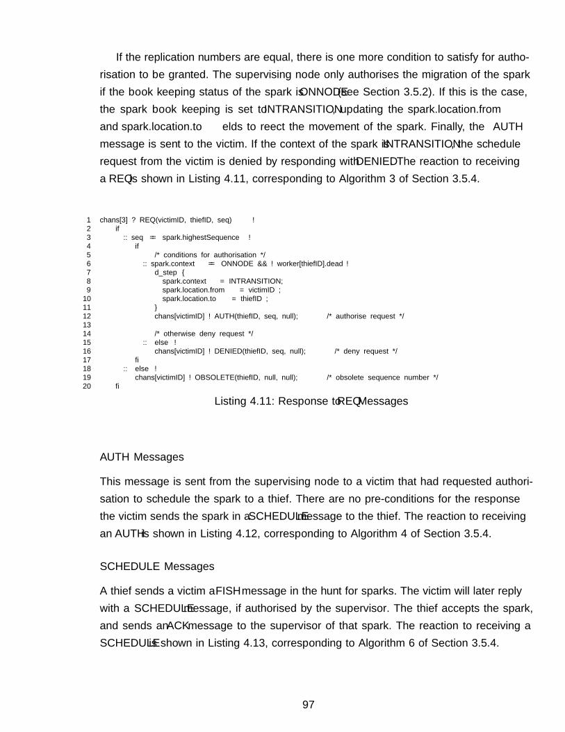
If the replication numbers are equal, there is one more condition to satisfy for autho-risation to be granted. The supervising node only authorises the migration of the sparkif the book keeping status of the spark is ONNODE (see Section 3.5.2). If this is the case,the spark book keeping is set to INTRANSITION, updating the spark.location.from

and spark.location.to fields to reflect the movement of the spark. Finally, the AUTH

message is sent to the victim. If the context of the spark is INTRANSITION, the schedulerequest from the victim is denied by responding with DENIED. The reaction to receivinga REQ is shown in Listing 4.11, corresponding to Algorithm 3 of Section 3.5.4.

1 chans[3] ? REQ(victimID, thiefID, seq) →2 if3 :: seq == spark.highestSequence →4 if5 /* conditions for authorisation */6 :: spark.context == ONNODE && ! worker[thiefID].dead→7 d_step {8 spark.context = INTRANSITION;9 spark.location.from = victimID ;

10 spark.location.to = thiefID ;11 }12 chans[victimID] ! AUTH(thiefID, seq, null); /* authorise request */1314 /* otherwise deny request */15 :: else →16 chans[victimID] ! DENIED(thiefID, seq, null); /* deny request */17 fi18 :: else →19 chans[victimID] ! OBSOLETE(thiefID, null, null); /* obsolete sequence number */20 fi

Listing 4.11: Response to REQ Messages

AUTH Messages

This message is sent from the supervising node to a victim that had requested authori-sation to schedule the spark to a thief. There are no pre-conditions for the response —the victim sends the spark in a SCHEDULE message to the thief. The reaction to receivingan AUTH is shown in Listing 4.12, corresponding to Algorithm 4 of Section 3.5.4.

SCHEDULE Messages

A thief sends a victim a FISH message in the hunt for sparks. The victim will later replywith a SCHEDULE message, if authorised by the supervisor. The thief accepts the spark,and sends an ACK message to the supervisor of that spark. The reaction to receiving aSCHEDULE is shown in Listing 4.13, corresponding to Algorithm 6 of Section 3.5.4.

97

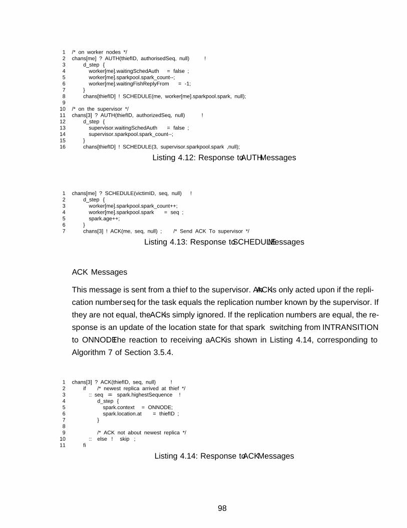
1 /* on worker nodes */2 chans[me] ? AUTH(thiefID, authorisedSeq, null) →3 d_step {4 worker[me].waitingSchedAuth = false;5 worker[me].sparkpool.spark_count--;6 worker[me].waitingFishReplyFrom = -1;7 }8 chans[thiefID] ! SCHEDULE(me, worker[me].sparkpool.spark, null);9

10 /* on the supervisor */11 chans[3] ? AUTH(thiefID, authorizedSeq, null) →12 d_step {13 supervisor.waitingSchedAuth = false;14 supervisor.sparkpool.spark_count--;15 }16 chans[thiefID] ! SCHEDULE(3, supervisor.sparkpool.spark ,null);

Listing 4.12: Response to AUTH Messages

1 chans[me] ? SCHEDULE(victimID, seq, null) →2 d_step {3 worker[me].sparkpool.spark_count++;4 worker[me].sparkpool.spark = seq ;5 spark.age++;6 }7 chans[3] ! ACK(me, seq, null) ; /* Send ACK To supervisor */

Listing 4.13: Response to SCHEDULE Messages

ACK Messages

This message is sent from a thief to the supervisor. An ACK is only acted upon if the repli-cation number seq for the task equals the replication number known by the supervisor. Ifthey are not equal, the ACK is simply ignored. If the replication numbers are equal, the re-sponse is an update of the location state for that spark — switching from INTRANSITION

to ONNODE. The reaction to receiving a ACK is shown in Listing 4.14, corresponding toAlgorithm 7 of Section 3.5.4.

1 chans[3] ? ACK(thiefID, seq, null) →2 if /* newest replica arrived at thief */3 :: seq == spark.highestSequence →4 d_step {5 spark.context = ONNODE;6 spark.location.at = thiefID ;7 }89 /* ACK not about newest replica */

10 :: else → skip ;11 fi

Listing 4.14: Response to ACK Messages

98

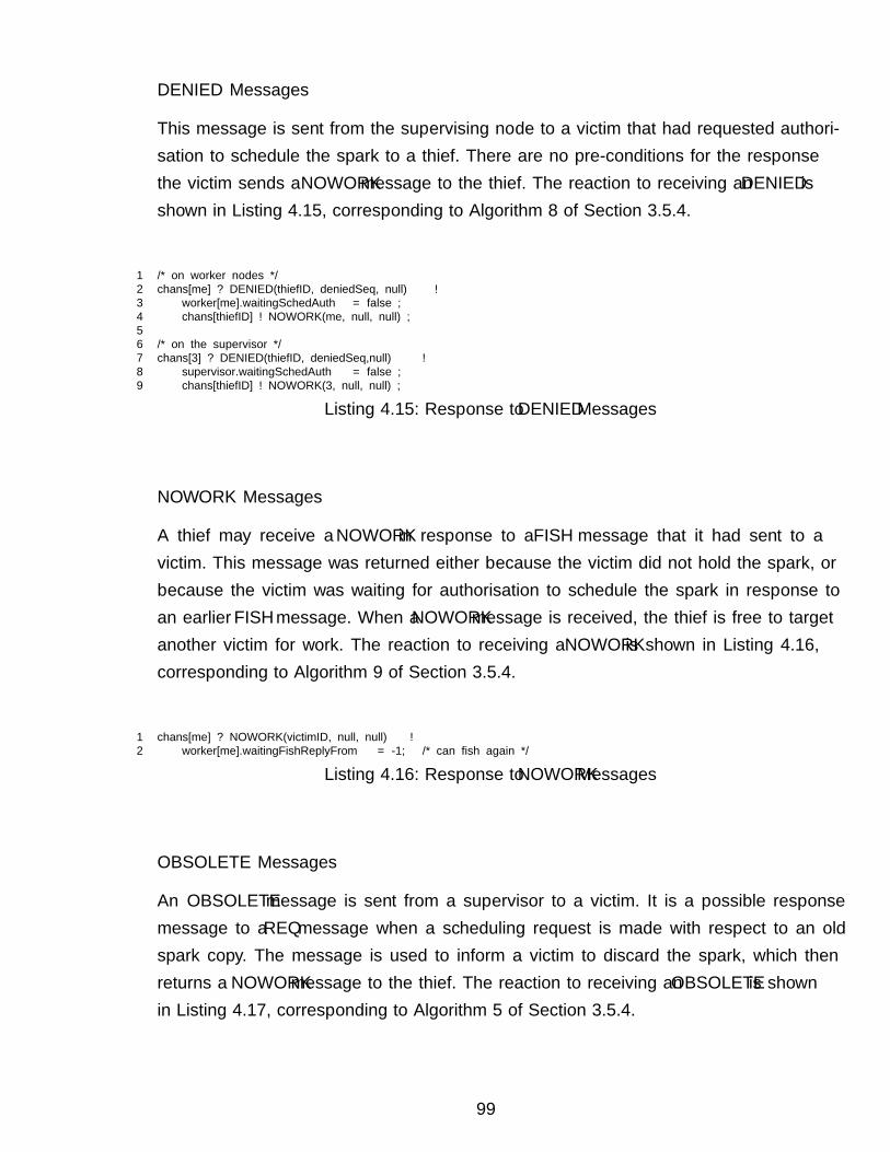
DENIED Messages

This message is sent from the supervising node to a victim that had requested authori-sation to schedule the spark to a thief. There are no pre-conditions for the response —the victim sends a NOWORK message to the thief. The reaction to receiving an DENIED isshown in Listing 4.15, corresponding to Algorithm 8 of Section 3.5.4.

1 /* on worker nodes */2 chans[me] ? DENIED(thiefID, deniedSeq, null) →3 worker[me].waitingSchedAuth = false;4 chans[thiefID] ! NOWORK(me, null, null) ;56 /* on the supervisor */7 chans[3] ? DENIED(thiefID, deniedSeq,null) →8 supervisor.waitingSchedAuth = false;9 chans[thiefID] ! NOWORK(3, null, null) ;

Listing 4.15: Response to DENIED Messages

NOWORK Messages

A thief may receive a NOWORK in response to a FISH message that it had sent to avictim. This message was returned either because the victim did not hold the spark, orbecause the victim was waiting for authorisation to schedule the spark in response toan earlier FISH message. When a NOWORK message is received, the thief is free to targetanother victim for work. The reaction to receiving a NOWORK is shown in Listing 4.16,corresponding to Algorithm 9 of Section 3.5.4.

1 chans[me] ? NOWORK(victimID, null, null) →2 worker[me].waitingFishReplyFrom = -1; /* can fish again */

Listing 4.16: Response to NOWORK Messages

OBSOLETE Messages

An OBSOLETE message is sent from a supervisor to a victim. It is a possible responsemessage to a REQ message when a scheduling request is made with respect to an oldspark copy. The message is used to inform a victim to discard the spark, which thenreturns a NOWORK message to the thief. The reaction to receiving an OBSOLETE is shownin Listing 4.17, corresponding to Algorithm 5 of Section 3.5.4.

99

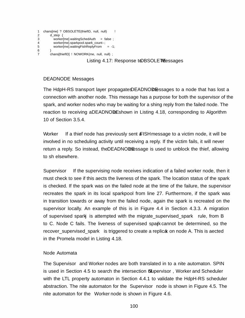
1 chans[me] ? OBSOLETE(thiefID, null, null) →2 d_step {3 worker[me].waitingSchedAuth = false;4 worker[me].sparkpool.spark_count--;5 worker[me].waitingFishReplyFrom = -1;6 }7 chans[thiefID] ! NOWORK(me, null, null) ;

Listing 4.17: Response to OBSOLETE Messages

DEADNODE Messages

The HdpH-RS transport layer propagates DEADNODE messages to a node that has lost aconnection with another node. This message has a purpose for both the supervisor of thespark, and worker nodes who may be waiting for a fishing reply from the failed node. Thereaction to receiving a DEADNODE is shown in Listing 4.18, corresponding to Algorithm10 of Section 3.5.4.

Worker If a thief node has previously sent a FISH message to a victim node, it will beinvolved in no scheduling activity until receiving a reply. If the victim fails, it will neverreturn a reply. So instead, the DEADNODE message is used to unblock the thief, allowingto fish elsewhere.

Supervisor If the supervising node receives indication of a failed worker node, then itmust check to see if this affects the liveness of the spark. The location status of the sparkis checked. If the spark was on the failed node at the time of the failure, the supervisorrecreates the spark in its local sparkpool from line 27. Furthermore, if the spark wasin transition towards or away from the failed node, again the spark is recreated on thesupervisor locally. An example of this is in Figure 4.4 in Section 4.3.3. A migrationof supervised spark j is attempted with the migrate_supervised_spark rule, from Bto C. Node C fails. The liveness of supervised spark j cannot be determined, so therecover_supervised_spark is triggered to create a replica k on node A. This is affectedin the Promela model in Listing 4.18.

Node Automata

The Supervisor and Worker nodes are both translated in to a finite automaton. SPINis used in Section 4.5 to search the intersection of Supervisor, Worker and Scheduler

with the LTL property automaton in Section 4.4.1 to validate the HdpH-RS schedulerabstraction. The finite automaton for the Supervisor node is shown in Figure 4.5. Thefinite automaton for the Worker node is shown in Figure 4.6.

100

Supe

rvis

orS1 S2su

perv

isor

.spa

rkpo

ol.s

park

_cou

nt =

1

S3

(run

Wor

ker(

0))

S4(r

un W

orke

r(1)

)

S86(run

Wor

ker(

2))

S9

(((s

uper

viso

r.spa

rkpo

ol.s

park

_cou

nt>0

)&&

(spa

rk.a

ge>1

00))

)

S84

else

S7

supe

rvis

or.re

sultS

ent =

1

S15

((su

perv

isor

.spa

rkpo

ol.s

park

_cou

nt>0

))

S17

chan

s[3]

?DEN

IED

,thie

fID

,den

iedS

eq,-1

S25

chan

s[3]

?FIS

H,th

iefI

D,-1

,-1

S30

chan

s[3]

?AU

TH,th

iefI

D,a

utho

rized

Seq,

-1

S46

chan

s[3]

?REQ

,vic

timID

,thie

fID

,seq

S55

chan

s[3]

?AC

K,th

iefI

D,s

eq,-1

S58

chan

s[3]

?RES

ULT

,-1,-1

,-1

S62

chan

s[3]

?DEA

DN

OD

E,de

adN

odeI

D,-1

,-1 S8

supe

rvis

or.iv

ar =

1

S13

supe

rvis

or.re

sultS

ent =

1

S18su

perv

isor

.wai

tingS

ched

Aut

h =

0

S21

(((s

uper

viso

r.spa

rkpo

ol.s

park

_cou

nt>0

)&&

!(su

perv

isor

.wai

tingS

ched

Aut

h)))

S24

else

S31

D_S

TEP

S42((se

q==s

park

.hig

hest

Rep

lica)

)

S45

else

S52

((se

q==s

park

.hig

hest

Rep

lica)

)

S54

else

S59

supe

rvis

or.iv

ar =

1

S83

shou

ld_r

eplic

ate

= 0

S94

goto

EV

ALU

ATI

ON

_CO

MPL

ETE

S14su

perv

isor

.ivar

= 1

S92

chan

s[th

iefI

D]!

NO

WO

RK

,3,-(

1),-(

1)

S22

supe

rvis

or.w

aitin

gSch

edA

uth

= 1

chan

s[th

iefI

D]!

NO

WO

RK

,3,-(

1),-(

1)

chan

s[th

iefI

D]!

SCH

EDU

LE,3

,sup

ervi

sor.s

park

pool

.spa

rk,-(

1)

S38

(((s

park

.con

text

==O

NN

OD

E)&

&!(

wor

ker[

thie

fID

].dea

d)))

S41

else

chan

s[vi

ctim

ID]!

OB

SOLE

TE,th

iefI

D,-(

1),-(

1)

D_S

TEP

(1)

goto

EV

ALU

ATI

ON

_CO

MPL

ETE

D_S

TEP

S95(1

)

S0-end

-

goto

EV

ALU

ATI

ON

_CO

MPL

ETE

((su

perv

isor

.ivar

==0)

)

S91

else

chan

s[3]

!REQ

,3,th

iefI

D,s

uper

viso

r.spa

rkpo

ol.s

park

S39

D_S

TEP

chan

s[vi

ctim

ID]!

DEN

IED

,thie

fID

,seq

,-(1)

(1)

chan

s[vi

ctim

ID]!

AU

TH,th

iefI

D,s

eq,-(

1)

Figu

re4.5:

Supe

rviso

rAutom

ata

101

Wor

ker

S74

S5

(((w

orke

r[m

e].s

park

pool

.spa

rk_c

ount

>0)&

&(s

park

.age

>100

)))

S72

else

S3wor

ker[

me]

.resu

ltSen

t = 1

S8

(1)

S16

((w

orke

r[m

e].s

park

pool

.spa

rk_c

ount

>0))

S18

((((

wor

ker[

me]

.spa

rkpo

ol.s

park

_cou

nt==

0)&

&(w

orke

r[m

e].w

aitin

gFis

hRep

lyFr

om==

-(1)

))&

&(s

park

.age

<(10

0+1)

)))

S34

chan

s[m

e]?N

OW

OR

K,v

ictim

ID,-1

,-1S4

1

chan

s[m

e]?F

ISH

,thie

fID

,-1,-1

S47ch

ans[

me]

?AU

TH

,thie

fID

,aut

hori

sedS

eq,-1

S50

chan

s[m

e]?D

EN

IED

,thie

fID

,den

iedS

eq,-1

S56

chan

s[m

e]?O

BSO

LE

TE

,thie

fID

,-1,-1

S62

chan

s[m

e]?S

CH

ED

UL

E,v

ictim

ID,s

eq,-1

S71

chan

s[m

e]?D

EA

DN

OD

E,d

eadN

odeI

D,-1

,-1

S4chan

s[3]

!RE

SUL

T,-(

1),-(

1),-(

1)

S13wor

ker[

me]

.dea

d =

1

S80

chan

s[3]

!RE

SUL

T,-(

1),-(

1),-(

1)

S31ch

osen

Vic

timID

= 0 w

orke

r[m

e].w

aitin

gFis

hRep

lyFr

om =

-(1)

S37

(((w

orke

r[m

e].s

park

pool

.spa

rk_c

ount

>0)&

&!(

wor

ker[

me]

.wai

tingS

ched

Aut

h)))

S40

else

S48

D_S

TE

P

S51

wor

ker[

me]

.wai

tingS

ched

Aut

h =

0

S57

D_S

TE

PS6

3

D_S

TE

P

D_S

TE

P

S82

goto

EN

DS10

chan

s[0]

!DE

AD

NO

DE

,me,

-(1)

,-(1)

((su

perv

isor

.ivar

==1)

)

else

S32

D_S

TE

P

S38

wor

ker[

me]

.wai

tingS

ched

Aut

h =

1

chan

s[th

iefI

D]!

NO

WO

RK

,me,

-(1)

,-(1)

chan

s[th

iefI

D]!

SCH

ED

UL

E,m

e,w

orke

r[m

e].s

park

pool

.spa

rk,-(

1)ch

ans[

thie

fID

]!N

OW

OR

K,m

e,-(

1),-(

1)ch

ans[

thie

fID

]!N

OW

OR

K,m

e,-(

1),-(

1)ch

ans[

3]!A

CK

,me,

seq,

-(1)

S83(1

)

S0-end

-

S11

chan

s[1]

!DE

AD

NO

DE

,me,

-(1)

,-(1)

chan

s[ch

osen

Vic

timID

]!FI

SH,m

e,-(

1),-(

1)ch

ans[

3]!R

EQ

,me,

thie

fID

,wor

ker[

me]

.spa

rkpo

ol.s

park

S12chan

s[2]

!DE

AD

NO

DE

,me,

-(1)

,-(1)

chan

s[3]

!DE

AD

NO

DE

,me,

-(1)

,-(1)

Figu

re4.6:

WorkerAutom

ata

102

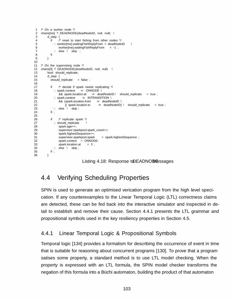
1 /* On a worker node */2 chans[me] ? DEADNODE(deadNodeID, null, null) →3 d_step {4 if /* reset to start fishing from other nodes */5 :: worker[me].waitingFishReplyFrom > deadNodeID →6 worker[me].waitingFishReplyFrom = -1 ;7 :: else → skip ;8 fi9 }

1011 /* On the supervising node */12 chans[3] ? DEADNODE(deadNodeID, null, null) →13 bool should_replicate;14 d_step {15 should_replicate = false;1617 if /* decide if spark needs replicating */18 :: spark.context == ONNODE \19 && spark.location.at == deadNodeID → should_replicate = true;20 :: spark.context == INTRANSITION \21 && (spark.location.from == deadNodeID \22 || spark.location.to == deadNodeID) → should_replicate = true;23 :: else → skip;24 fi;2526 if /* replicate spark */27 :: should_replicate →28 spark.age++;29 supervisor.sparkpool.spark_count++;30 spark.highestSequence++;31 supervisor.sparkpool.spark = spark.highestSequence ;32 spark.context = ONNODE;33 spark.location.at = 3 ;34 :: else → skip;35 fi;36 }

Listing 4.18: Response to DEADNODE Messages

4.4 Verifying Scheduling Properties

SPIN is used to generate an optimised verification program from the high level specifi-cation. If any counterexamples to the Linear Temporal Logic (LTL) correctness claimsare detected, these can be fed back into the interactive simulator and inspected in de-tail to establish and remove their cause. Section 4.4.1 presents the LTL grammar andpropositional symbols used in the key resiliency properties in Section 4.5.

4.4.1 Linear Temporal Logic & Propositional Symbols

Temporal logic [134] provides a formalism for describing the occurrence of event in timethat is suitable for reasoning about concurrent programs [130]. To prove that a programsatisfies some property, a standard method is to use LTL model checking. When theproperty is expressed with an LTL formula, the SPIN model checker transforms thenegation of this formula into a Büchi automaton, building the product of that automaton

103

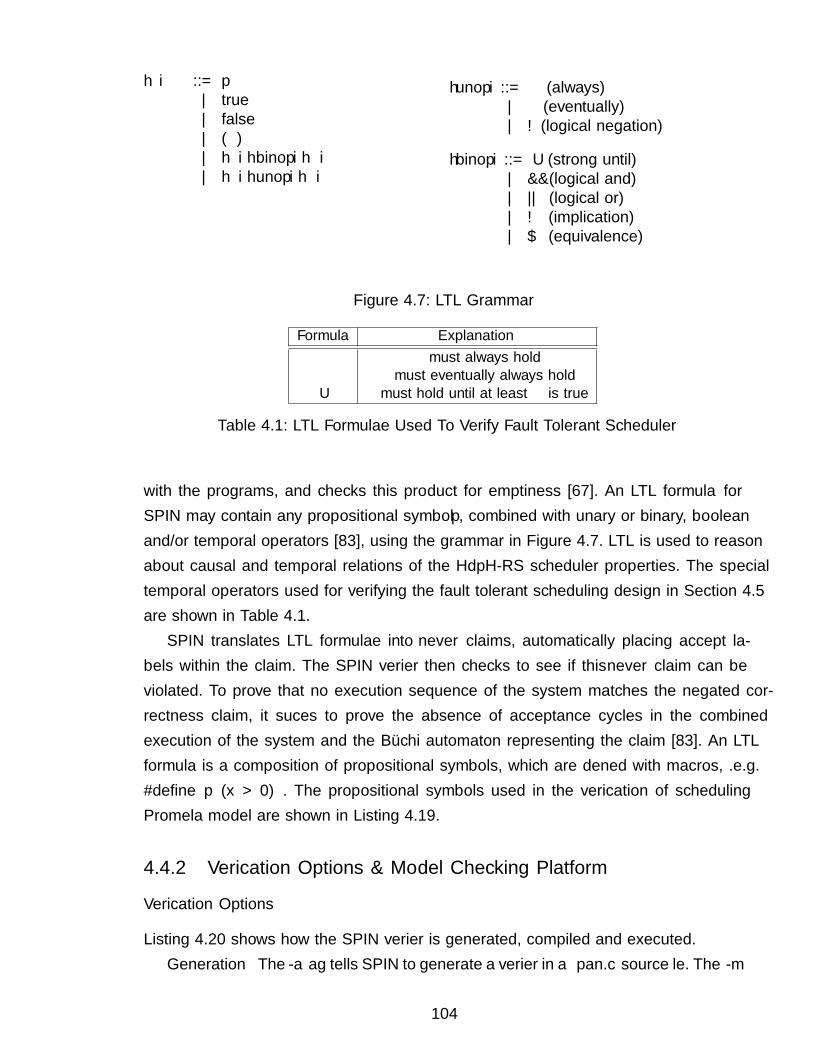
〈φ〉 ::= p| true| false| (φ)| 〈ψ〉 〈binop〉 〈φ〉| 〈ψ〉 〈unop〉 〈φ〉

〈unop〉 ::= � (always)| ♦ (eventually)| ! (logical negation)

〈binop〉 ::= U (strong until)| && (logical and)| || (logical or)| → (implication)| ↔ (equivalence)

Figure 4.7: LTL Grammar

Formula Explanation�φ φ must always hold♦�φ φ must eventually always holdψ U φ ψ must hold until at least φ is true

Table 4.1: LTL Formulae Used To Verify Fault Tolerant Scheduler

with the programs, and checks this product for emptiness [67]. An LTL formula φ forSPIN may contain any propositional symbol p, combined with unary or binary, booleanand/or temporal operators [83], using the grammar in Figure 4.7. LTL is used to reasonabout causal and temporal relations of the HdpH-RS scheduler properties. The specialtemporal operators used for verifying the fault tolerant scheduling design in Section 4.5are shown in Table 4.1.

SPIN translates LTL formulae into never claims, automatically placing accept la-bels within the claim. The SPIN verifier then checks to see if this never claim can beviolated. To prove that no execution sequence of the system matches the negated cor-rectness claim, it suffices to prove the absence of acceptance cycles in the combinedexecution of the system and the Büchi automaton representing the claim [83]. An LTLformula is a composition of propositional symbols, which are defined with macros, .e.g.#define p (x > 0). The propositional symbols used in the verification of schedulingPromela model are shown in Listing 4.19.

4.4.2 Verification Options & Model Checking Platform

Verification Options

Listing 4.20 shows how the SPIN verifier is generated, compiled and executed.Generation The -a flag tells SPIN to generate a verifier in a pan.c source file. The -m

104

1 /* IVar on the supervisor node is full */2 #define ivar_full ( supervisor.ivar == 1 )34 /* IVar on the supervisor node is empty */5 #define ivar_empty ( supervisor.ivar == 0 )67 /* No worker nodes have failed */8 #define all_workers_alive ( !worker[0].dead && !worker[1].dead && !worker[2].dead )9

10 /* One or more nodes have transmitted a value to supervisor to fill IVar */11 #define any_result_sent ( supervisor.resultSent12 || worker[0].resultSent13 || worker[1].resultSent14 || worker[2].resultSent )

Listing 4.19: Propositional Symbols used in LTL Formulae of Fault Tolerant Properties

1 $ spin -a -m hdph-rs.pml2 $ gcc -DMEMLIM=1024 -O2 -DXUSAFE -DCOLLAPSE -w -o pan pan.c3 $ ./pan -m10000 -E -a -f -c1 -N never_2

Listing 4.20: Compiling & Executing SPIN Verifier

flag tells SPIN to lose messages sent to full channel buffers. This reflects the impossibilityof filling a TCP receive buffer on a dead HdpH-RS node. The -m flag prevents healthynodes from blocking of full channels in the model.

Compilation The memory limit is set to 1024Mb with the -DMEMLIM flag. Checksfor channel assertion violations are disabled with -DXUSAFE, as they are not used. The-DCOLLAPSE flag enables state vector compression.

Verification The maximum search space is set to 10000 with the -m flag, and amaximum of 124 is used. The -a flag tells SPIN to check for acceptance cycles in theLTL property automata. Weak fairness is enabled with the -f flag. The -E flag suppressesthe reporting of invalid end states. This ensures that every statement always enabled froma certain point is eventually executed. The verification ends after finding the first errorwith the -c flag. The -N flag selects the LTL property to be verified.

4.5 Model Checking Results

This section reports the results of SPIN verification. The results of model checking thethree LTL properties are in Table 4.2. Taking the ♦ � ivar_full property as an example,the results can be interpreted as follows. A reachable depth of 124 is found by SPIN forthe model. The reachable state space is 8.2 million. A total of 22.4 million transitionswere explored in the search. Actual memory usage for states was 84.7Mb.

105

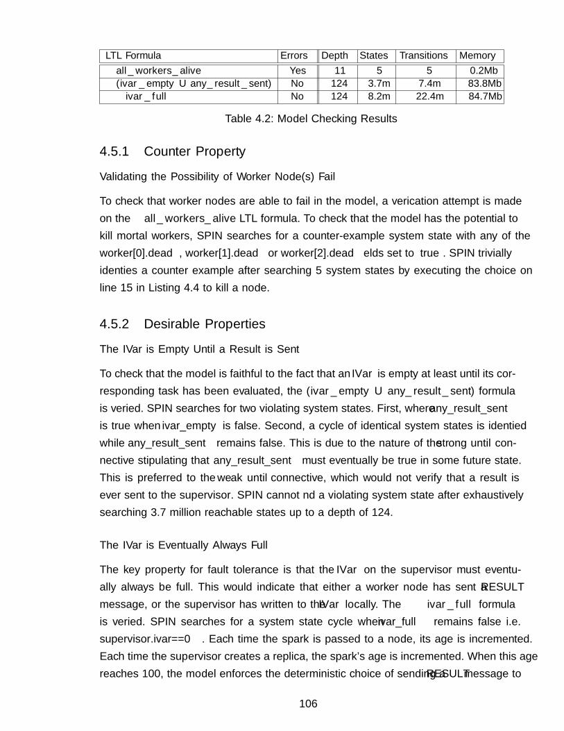
LTL Formula Errors Depth States Transitions Memory� all_workers_alive Yes 11 5 5 0.2Mb� (ivar_empty U any_result_sent) No 124 3.7m 7.4m 83.8Mb♦ � ivar_full No 124 8.2m 22.4m 84.7Mb

Table 4.2: Model Checking Results

4.5.1 Counter Property

Validating the Possibility of Worker Node(s) Fail

To check that worker nodes are able to fail in the model, a verification attempt is madeon the � all_workers_alive LTL formula. To check that the model has the potential tokill mortal workers, SPIN searches for a counter-example system state with any of theworker[0].dead, worker[1].dead or worker[2].dead fields set to true. SPIN triviallyidentifies a counter example after searching 5 system states by executing the choice online 15 in Listing 4.4 to kill a node.

4.5.2 Desirable Properties

The IVar is Empty Until a Result is Sent

To check that the model is faithful to the fact that an IVar is empty at least until its cor-responding task has been evaluated, the � (ivar_empty U any_result_sent) formulais verified. SPIN searches for two violating system states. First, where any_result_sentis true when ivar_empty is false. Second, a cycle of identical system states is identifiedwhile any_result_sent remains false. This is due to the nature of the strong until con-nective stipulating that any_result_sent must eventually be true in some future state.This is preferred to the weak until connective, which would not verify that a result isever sent to the supervisor. SPIN cannot find a violating system state after exhaustivelysearching 3.7 million reachable states up to a depth of 124.

The IVar is Eventually Always Full

The key property for fault tolerance is that the IVar on the supervisor must eventu-ally always be full. This would indicate that either a worker node has sent a RESULT

message, or the supervisor has written to the IVar locally. The ♦ � ivar_full formulais verified. SPIN searches for a system state cycle when ivar_full remains false i.e.supervisor.ivar==0. Each time the spark is passed to a node, its age is incremented.Each time the supervisor creates a replica, the spark’s age is incremented. When this agereaches 100, the model enforces the deterministic choice of sending a RESULT message to

106

the supervisor on any nodes that hold a replica, representing rput calls in HdpH-RS.The supervisor sets supervisor.ivar to 1 when it receives a RESULT message.

This LTL property checks for the fatal scenario when the supervisor does not repli-cate the spark in the model, when it must in order to ensure the existence of at leastone replica. This would happen if the HdpH-RS fault tolerant fishing protocol algorithm(Section 3.5.4) did not catch corner cases whereby spark location tracking becomes invali-dated. The consequence would be the supervisor’s incorrect decision not to replication thespark when a DEADNODE message is received. Should the location tracking be invalidatedand the dead node held the only replica, no nodes would ever be able to send a RESULT

message to the supervisor. SPIN therefore searches for states where the spark_count

value is 0 for all nodes, and the supervisor does not create a replica in any future state.SPIN cannot find a violating system state after exhaustively searching 8.2 million reach-able states up to a depth of 124.

4.6 Identifying Scheduling Bugs

SPIN identified bugs in the fault tolerant scheduling algorithm (Section 3.5.4), whichwere abstracted into earlier iterations of the Promela model. This section describes oneof many examples of how SPIN identified transitions to violating states with respect tothe ♦ � ivar_full property. Each bug was removed with modifications to the schedulingalgorithm (Section 3.5.4), and corresponding fixes in the Haskell scheduler implementa-tion (Chapter 5). With respect to the bug described here, the fix to the Promela modeland the Haskell implementation is shown in Appendix A.4.

The Bug

The LTL formula <> [] ivar_full claims that the empty IVar is eventually always full.Attempting to verify this property uncovered a corner case that would lead to deadlockand an IVar would never been filled with a value. There were insufficient pre-conditionsfor sending an AUTH message from a supervisor, in an earlier version of the model. Thecounter example that SPIN generated is shown in Figure 4.8. The supervisor node A willnot receive another DEADNODE message about node C after sending the AUTH message, sothe supervised spark would not be recovered and the IVar will never by filled.

The Fix

The fix was to add an additional guard on the supervisor, before sending an AUTH to thevictim (line 6 of Listing 4.11). Each REQ message includes a parameter stating who the

107

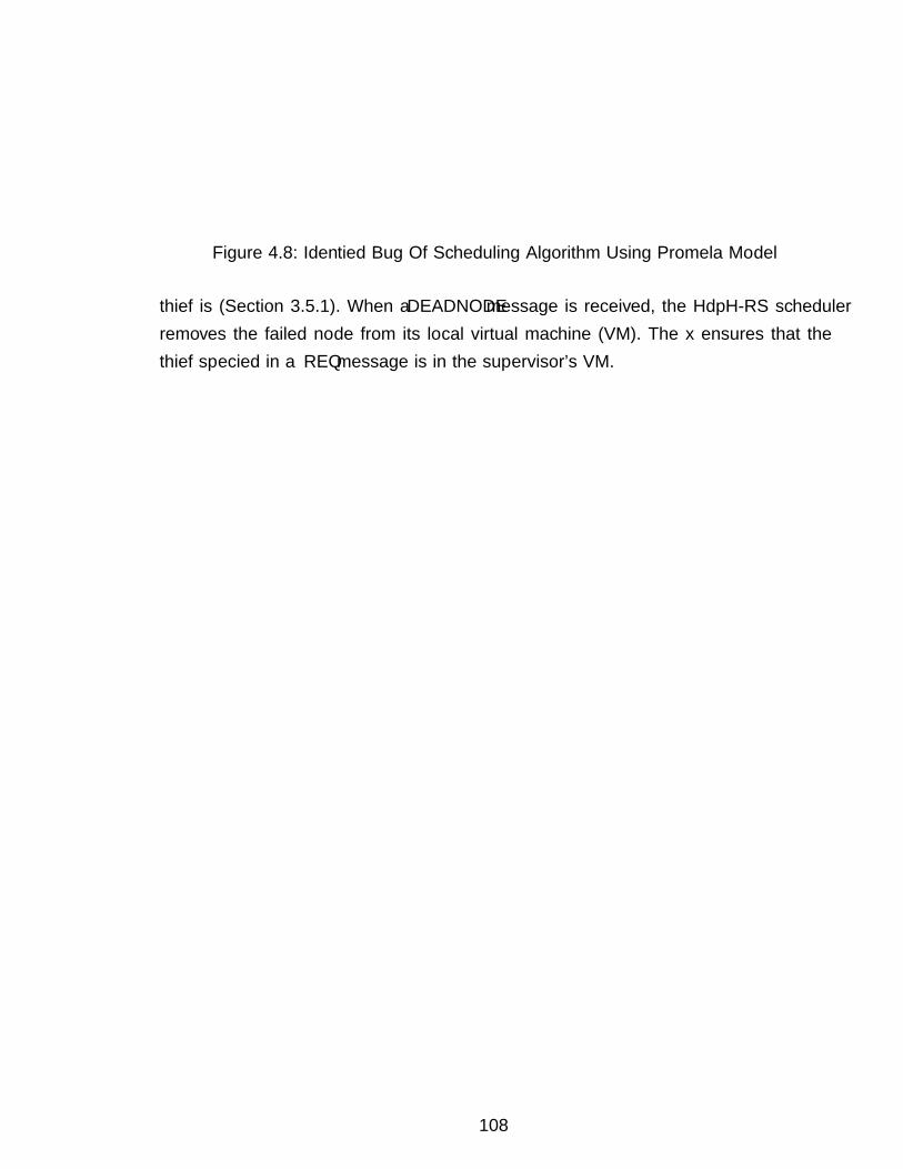
Node Asupervisor

Node Bvictim

Node Cthief

OnNode B FISH

DEADNODE CREQ

AUTH

InTransition B C SCHEDULE

Figure 4.8: Identified Bug Of Scheduling Algorithm Using Promela Model

thief is (Section 3.5.1). When a DEADNODE message is received, the HdpH-RS schedulerremoves the failed node from its local virtual machine (VM). The fix ensures that thethief specified in a REQ message is in the supervisor’s VM.

108

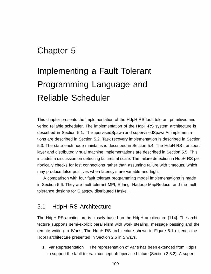
Chapter 5

Implementing a Fault TolerantProgramming Language andReliable Scheduler

This chapter presents the implementation of the HdpH-RS fault tolerant primitives andverified reliable scheduler. The implementation of the HdpH-RS system architecture isdescribed in Section 5.1. The supervisedSpawn and supervisedSpawnAt implementa-tions are described in Section 5.2. Task recovery implementation is described in Section5.3. The state each node maintains is described in Section 5.4. The HdpH-RS transportlayer and distributed virtual machine implementations are described in Section 5.5. Thisincludes a discussion on detecting failures at scale. The failure detection in HdpH-RS pe-riodically checks for lost connections rather than assuming failure with timeouts, whichmay produce false positives when latency’s are variable and high.

A comparison with four fault tolerant programming model implementations is madein Section 5.6. They are fault tolerant MPI, Erlang, Hadoop MapReduce, and the faulttolerance designs for Glasgow distributed Haskell.

5.1 HdpH-RS Architecture

The HdpH-RS architecture is closely based on the HdpH architecture [114]. The archi-tecture supports semi-explicit parallelism with work stealing, message passing and theremote writing to IVars. The HdpH-RS architecture shown in Figure 5.1 extends theHdpH architecture presented in Section 2.6 in 5 ways.

1. IVar Representation The representation of IVars has been extended from HdpHto support the fault tolerant concept of supervised futures (Section 3.3.2). A super-

109

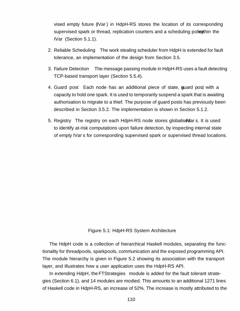
vised empty future (IVar) in HdpH-RS stores the location of its correspondingsupervised spark or thread, replication counters and a scheduling policy within theIVar (Section 5.1.1).

2. Reliable Scheduling The work stealing scheduler from HdpH is extended for faulttolerance, an implementation of the design from Section 3.5.

3. Failure Detection The message passing module in HdpH-RS uses a fault detectingTCP-based transport layer (Section 5.5.4).

4. Guard post Each node has an additional piece of state, a guard post, with acapacity to hold one spark. It is used to temporarily suspend a spark that is awaitingauthorisation to migrate to a thief. The purpose of guard posts has previously beendescribed in Section 3.5.2. The implementation is shown in Section 5.1.2.

5. Registry The registry on each HdpH-RS node stores globalised IVars. It is usedto identify at-risk computations upon failure detection, by inspecting internal stateof empty IVars for corresponding supervised spark or supervised thread locations.

scheduler scheduler

Node 1

IO threads IO threads

Node 2

thread pools

node table

msg handler

scheduler

msg handler

registry IVars

thread pools

Haskell heaps

TCP network

registry IVars node table

guard post guard postspark poolspark pool

Figure 5.1: HdpH-RS System Architecture

The HdpH code is a collection of hierarchical Haskell modules, separating the func-tionality for threadpools, sparkpools, communication and the exposed programming API.The module hierarchy is given in Figure 5.2 showing its association with the transportlayer, and illustrates how a user application uses the HdpH-RS API.

In extending HdpH, the FTStrategies module is added for the fault tolerant strate-gies (Section 6.1), and 14 modules are modified. This amounts to an additional 1271 linesof Haskell code in HdpH-RS, an increase of 52%. The increase is mostly attributed to the

110

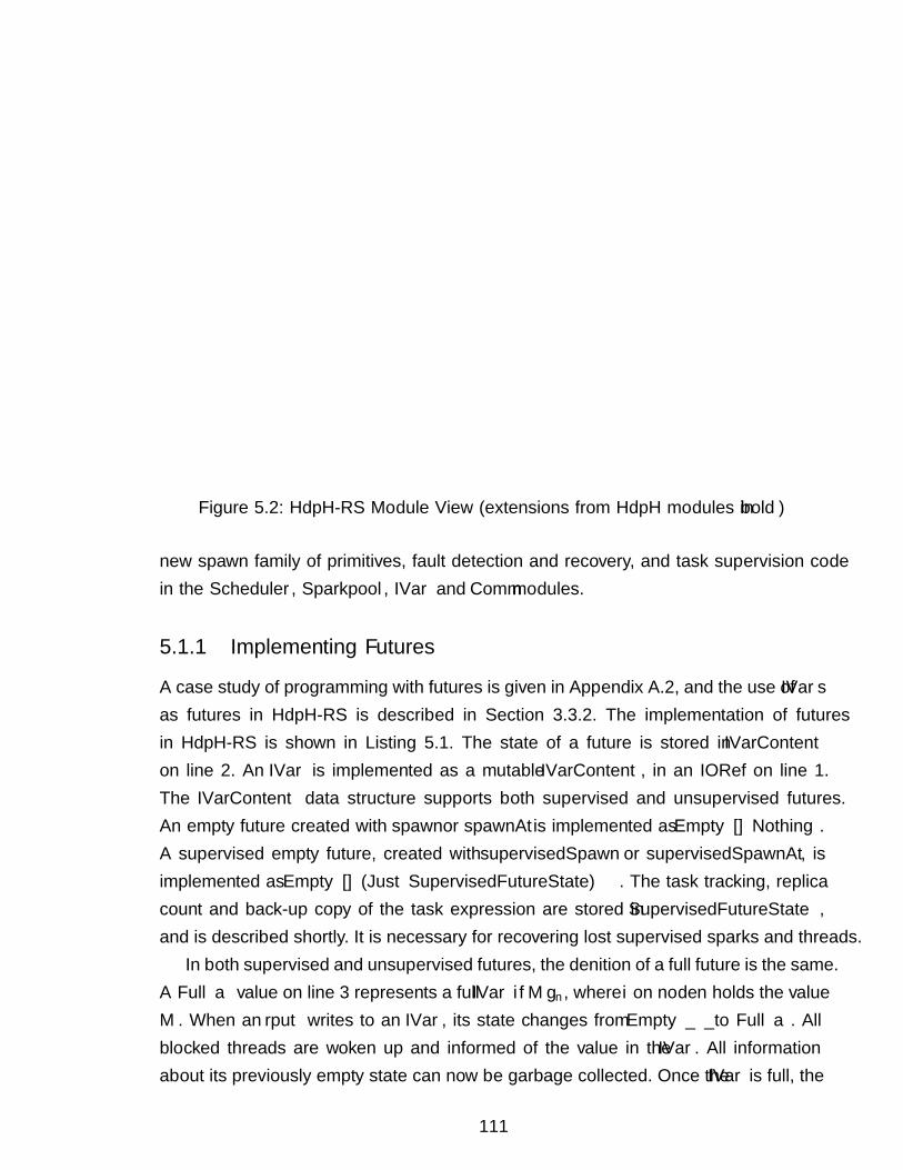
Sparkpool

Comm

Location

IVar

Scheduler

Internal

Network

TransportTCP

UserApplication

Threadpool

* Node to node message passing

* Thread work stealing

* Lazy spark distribution

* Handles: * FISH

* SCHEDULE* NOWORK

* OBSOLETE* ACK* AUTH* DENIED* REQ

* Connection loss detection

* Future representation: * Full * Empty

* Task copy * Location tracking

* Replica number

* Thread creation* Eager task distribution* Handles: * PUSH

* Guard post

HdpH−RS API

* supervisedSpawn

* supervisedSpawnAt* spawnAt

* spawn

* get * probe

* DEADNODE

HdpH−RS

FT−Strategies

Control

Parallel

HdpH−RS

* Task ACKnowledgement

Fault Tolerant Skeletons* parMap

*parDivideAndConquer

* MapReduceThres

* In total 11 skeletons

Figure 5.2: HdpH-RS Module View (extensions from HdpH modules in bold)

new spawn family of primitives, fault detection and recovery, and task supervision codein the Scheduler, Sparkpool, IVar and Comm modules.

5.1.1 Implementing Futures

A case study of programming with futures is given in Appendix A.2, and the use of IVarsas futures in HdpH-RS is described in Section 3.3.2. The implementation of futuresin HdpH-RS is shown in Listing 5.1. The state of a future is stored in IVarContent

on line 2. An IVar is implemented as a mutable IVarContent, in an IORef on line 1.The IVarContent data structure supports both supervised and unsupervised futures.An empty future created with spawn or spawnAt is implemented as Empty [] Nothing.A supervised empty future, created with supervisedSpawn or supervisedSpawnAt, isimplemented as Empty [] (Just SupervisedFutureState). The task tracking, replicacount and back-up copy of the task expression are stored in SupervisedFutureState,and is described shortly. It is necessary for recovering lost supervised sparks and threads.

In both supervised and unsupervised futures, the definition of a full future is the same.A Full a value on line 3 represents a full IVar i{M}n, where i on node n holds the valueM . When an rput writes to an IVar, its state changes from Empty _ _ to Full a. Allblocked threads are woken up and informed of the value in the IVar. All informationabout its previously empty state can now be garbage collected. Once the IVar is full, the

111

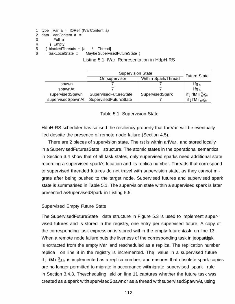
1 type IVar a = IORef (IVarContent a)2 data IVarContent a =3 Full a4 | Empty5 { blockedThreads :: [a → Thread]6 , taskLocalState :: Maybe SupervisedFutureState }

Listing 5.1: IVar Representation in HdpH-RS

Supervision State Future StateOn supervisor Within Spark/Threadspawn 7 7 i{}n

spawnAt 7 7 i{}nsupervisedSpawn SupervisedFutureState SupervisedSpark i{j〈〈M〉〉Sn′}nsupervisedSpawnAt SupervisedFutureState 7 i{j〈M〉n′}n

Table 5.1: Supervision State

HdpH-RS scheduler has satisfied the resiliency property that the IVar will be eventuallyfilled despite the presence of remote node failure (Section 4.5).

There are 2 pieces of supervision state. The first is within an IVar, and stored locallyin a SupervisedFuturesState structure. The atomic states in the operational semanticsin Section 3.4 show that of all task states, only supervised sparks need additional staterecording a supervised spark’s location and its replica number. Threads that correspondto supervised threaded futures do not travel with supervision state, as they cannot mi-grate after being pushed to the target node. Supervised futures and supervised sparkstate is summarised in Table 5.1. The supervision state within a supervised spark is laterpresented as SupervisedSpark in Listing 5.5.

Supervised Empty Future State

The SupervisedFutureState data structure in Figure 5.3 is used to implement super-vised futures and is stored in the registry, one entry per supervised future. A copy ofthe corresponding task expression is stored within the empty future as task on line 13.When a remote node failure puts the liveness of the corresponding task in jeopardy, taskis extracted from the empty IVar and rescheduled as a replica. The replication numberreplica on line 8 in the registry is incremented. The j value in a supervised futurei{j〈〈M〉〉Sn′}n is implemented as a replica number, and ensures that obsolete spark copiesare no longer permitted to migrate in accordance with migrate_supervised_spark rulein Section 3.4.3. The scheduling field on line 11 captures whether the future task wascreated as a spark with supervisedSpawn or as a thread with supervisedSpawnAt, using

112

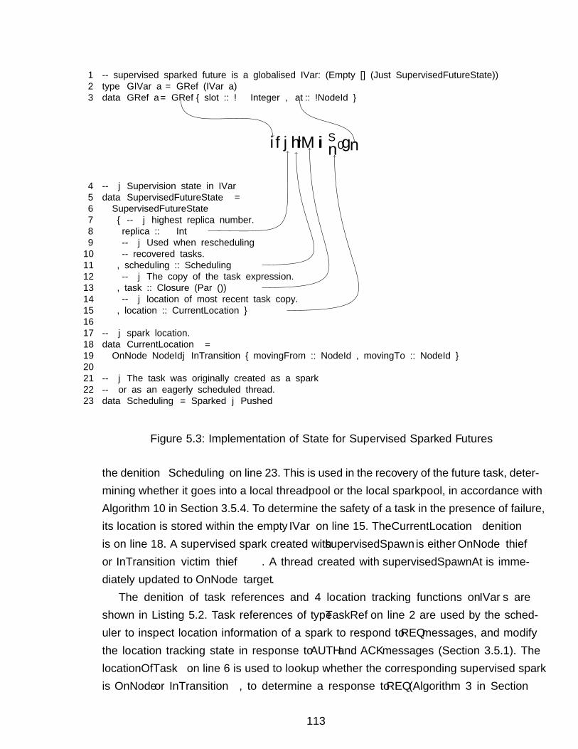
1 -- supervised sparked future is a globalised IVar: (Empty [] (Just SupervisedFutureState))2 type GIVar a = GRef (IVar a)3 data GRef a = GRef { slot :: !Integer, at:: !NodeId }

i{j〈〈M〉〉Sn′}n

4 -- | Supervision state in IVar5 data SupervisedFutureState =6 SupervisedFutureState7 { -- | highest replica number.8 replica :: Int9 -- | Used when rescheduling10 -- recovered tasks.11 , scheduling :: Scheduling12 -- | The copy of the task expression.13 , task :: Closure (Par ())14 -- | location of most recent task copy.15 , location :: CurrentLocation }1617 -- | spark location.18 data CurrentLocation =19 OnNode NodeId | InTransition { movingFrom :: NodeId , movingTo :: NodeId }2021 -- | The task was originally created as a spark22 -- or as an eagerly scheduled thread.23 data Scheduling = Sparked | Pushed

Figure 5.3: Implementation of State for Supervised Sparked Futures

the definition Scheduling on line 23. This is used in the recovery of the future task, deter-mining whether it goes into a local threadpool or the local sparkpool, in accordance withAlgorithm 10 in Section 3.5.4. To determine the safety of a task in the presence of failure,its location is stored within the empty IVar on line 15. The CurrentLocation definitionis on line 18. A supervised spark created with supervisedSpawn is either OnNode thief

or InTransition victim thief. A thread created with supervisedSpawnAt is imme-diately updated to OnNode target.

The definition of task references and 4 location tracking functions on IVars areshown in Listing 5.2. Task references of type TaskRef on line 2 are used by the sched-uler to inspect location information of a spark to respond to REQ messages, and modifythe location tracking state in response to AUTH and ACK messages (Section 3.5.1). ThelocationOfTask on line 6 is used to lookup whether the corresponding supervised sparkis OnNode or InTransition, to determine a response to REQ (Algorithm 3 in Section

113

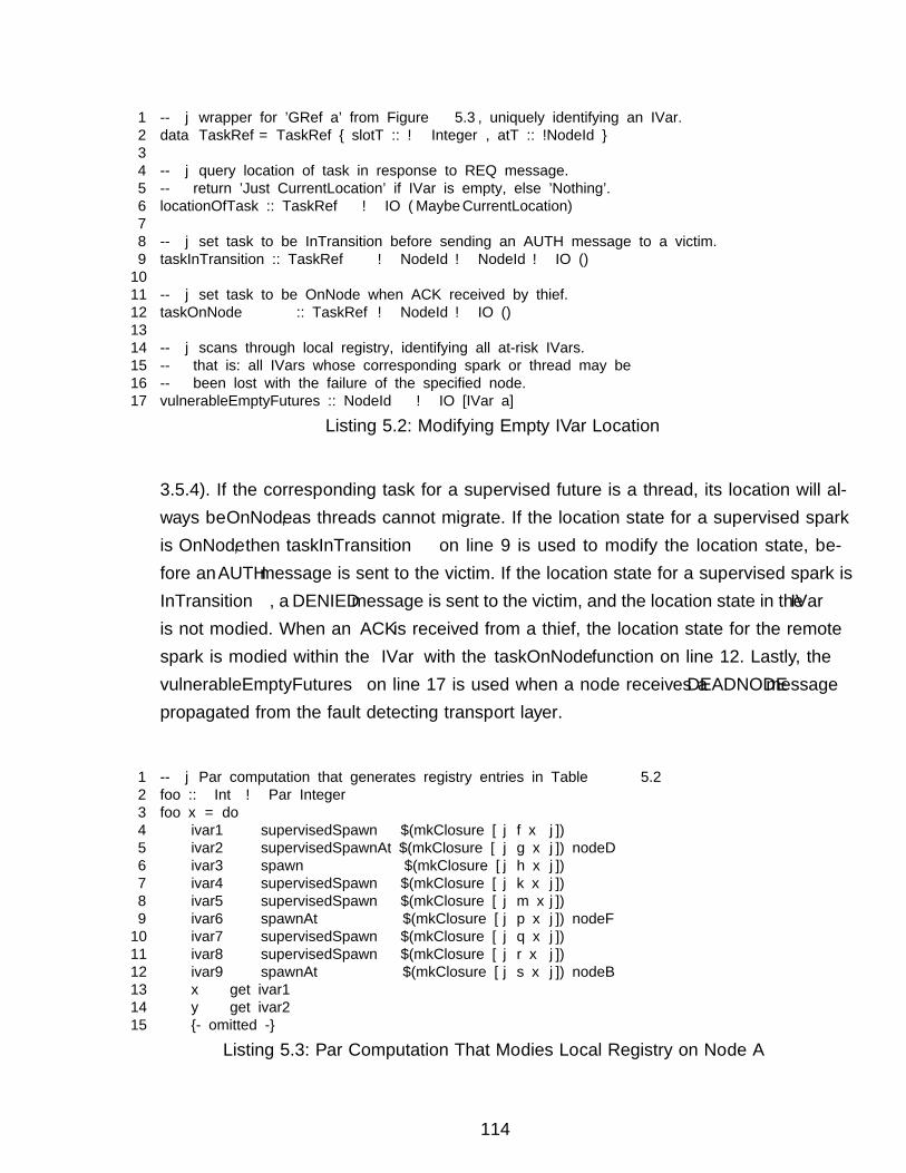
1 -- | wrapper for ’GRef a’ from Figure 5.3, uniquely identifying an IVar.2 data TaskRef = TaskRef { slotT :: !Integer, atT :: !NodeId }34 -- | query location of task in response to REQ message.5 -- return ’Just CurrentLocation’ if IVar is empty, else ’Nothing’.6 locationOfTask :: TaskRef → IO (Maybe CurrentLocation)78 -- | set task to be InTransition before sending an AUTH message to a victim.9 taskInTransition :: TaskRef → NodeId → NodeId → IO ()1011 -- | set task to be OnNode when ACK received by thief.12 taskOnNode :: TaskRef → NodeId → IO ()1314 -- | scans through local registry, identifying all at-risk IVars.15 -- that is: all IVars whose corresponding spark or thread may be16 -- been lost with the failure of the specified node.17 vulnerableEmptyFutures :: NodeId → IO [IVar a]

Listing 5.2: Modifying Empty IVar Location

3.5.4). If the corresponding task for a supervised future is a thread, its location will al-ways be OnNode, as threads cannot migrate. If the location state for a supervised sparkis OnNode, then taskInTransition on line 9 is used to modify the location state, be-fore an AUTH message is sent to the victim. If the location state for a supervised spark isInTransition, a DENIED message is sent to the victim, and the location state in the IVaris not modified. When an ACK is received from a thief, the location state for the remotespark is modified within the IVar with the taskOnNode function on line 12. Lastly, thevulnerableEmptyFutures on line 17 is used when a node receives a DEADNODE messagepropagated from the fault detecting transport layer.

1 -- | Par computation that generates registry entries in Table 5.22 foo :: Int → Par Integer3 foo x = do4 ivar1 ← supervisedSpawn $(mkClosure [ | f x |])5 ivar2 ← supervisedSpawnAt $(mkClosure [ | g x |]) nodeD6 ivar3 ← spawn $(mkClosure [ | h x |])7 ivar4 ← supervisedSpawn $(mkClosure [ | k x |])8 ivar5 ← supervisedSpawn $(mkClosure [ | m x |])9 ivar6 ← spawnAt $(mkClosure [ | p x |]) nodeF10 ivar7 ← supervisedSpawn $(mkClosure [ | q x |])11 ivar8 ← supervisedSpawn $(mkClosure [ | r x |])12 ivar9 ← spawnAt $(mkClosure [ | s x |]) nodeB13 x ← get ivar114 y ← get ivar215 {- omitted -}

Listing 5.3: Par Computation That Modifies Local Registry on Node A

114

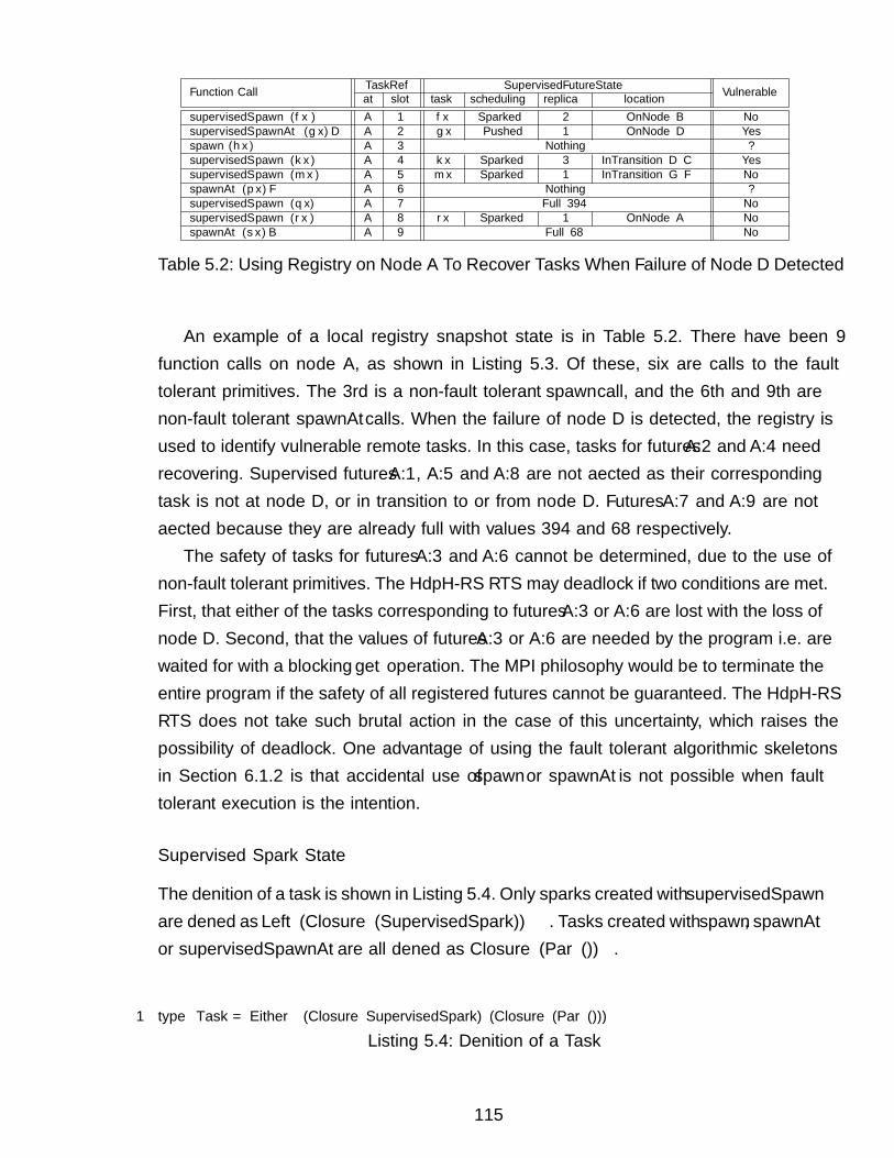
Function Call TaskRef SupervisedFutureState Vulnerableat slot task scheduling replica locationsupervisedSpawn (f x) A 1 f x Sparked 2 OnNode B NosupervisedSpawnAt (g x) D A 2 g x Pushed 1 OnNode D Yesspawn (h x) A 3 Nothing ?supervisedSpawn (k x) A 4 k x Sparked 3 InTransition D C YessupervisedSpawn (m x) A 5 m x Sparked 1 InTransition G F NospawnAt (p x) F A 6 Nothing ?supervisedSpawn (q x) A 7 Full 394 NosupervisedSpawn (r x) A 8 r x Sparked 1 OnNode A NospawnAt (s x) B A 9 Full 68 No

Table 5.2: Using Registry on Node A To Recover Tasks When Failure of Node D Detected

An example of a local registry snapshot state is in Table 5.2. There have been 9function calls on node A, as shown in Listing 5.3. Of these, six are calls to the faulttolerant primitives. The 3rd is a non-fault tolerant spawn call, and the 6th and 9th arenon-fault tolerant spawnAt calls. When the failure of node D is detected, the registry isused to identify vulnerable remote tasks. In this case, tasks for futures A:2 and A:4 needrecovering. Supervised futures A:1, A:5 and A:8 are not affected as their correspondingtask is not at node D, or in transition to or from node D. Futures A:7 and A:9 are notaffected because they are already full with values 394 and 68 respectively.

The safety of tasks for futures A:3 and A:6 cannot be determined, due to the use ofnon-fault tolerant primitives. The HdpH-RS RTS may deadlock if two conditions are met.First, that either of the tasks corresponding to futures A:3 or A:6 are lost with the loss ofnode D. Second, that the values of futures A:3 or A:6 are needed by the program i.e. arewaited for with a blocking get operation. The MPI philosophy would be to terminate theentire program if the safety of all registered futures cannot be guaranteed. The HdpH-RSRTS does not take such brutal action in the case of this uncertainty, which raises thepossibility of deadlock. One advantage of using the fault tolerant algorithmic skeletonsin Section 6.1.2 is that accidental use of spawn or spawnAt is not possible when faulttolerant execution is the intention.

Supervised Spark State

The definition of a task is shown in Listing 5.4. Only sparks created with supervisedSpawnare defined as Left (Closure (SupervisedSpark)). Tasks created with spawn, spawnAtor supervisedSpawnAt are all defined as Closure (Par ()).

1 type Task = Either (Closure SupervisedSpark) (Closure (Par ()))

Listing 5.4: Definition of a Task

115

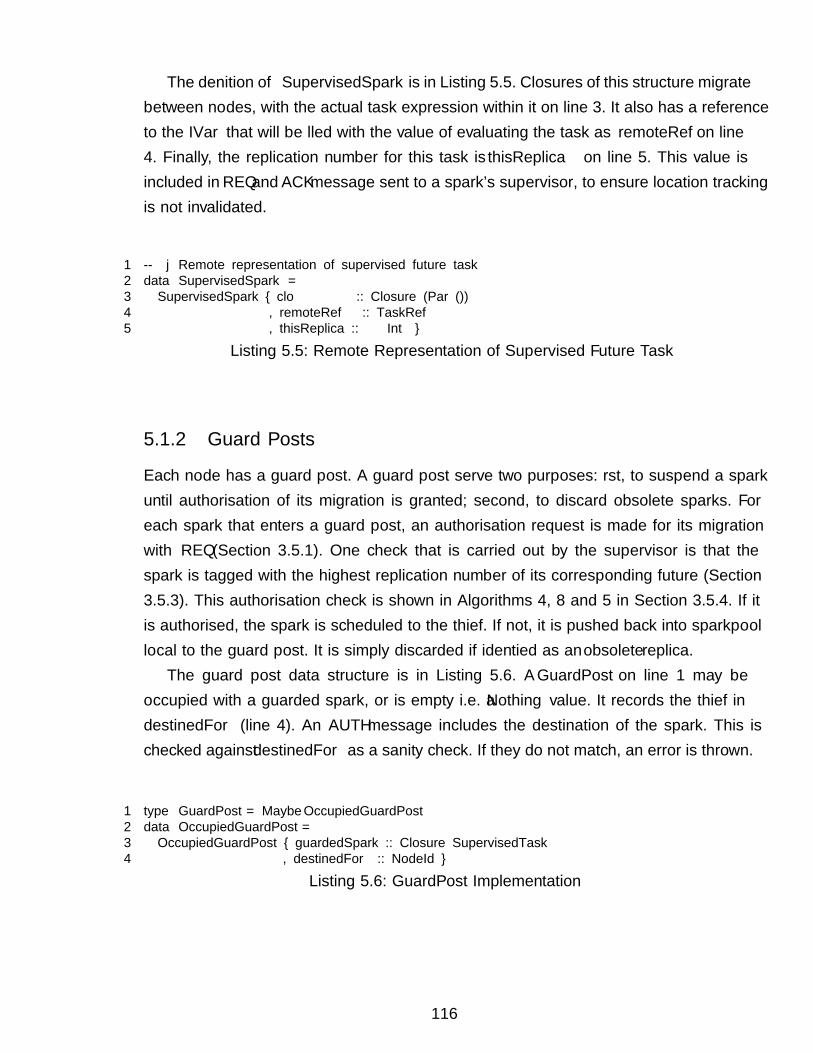
The definition of SupervisedSpark is in Listing 5.5. Closures of this structure migratebetween nodes, with the actual task expression within it on line 3. It also has a referenceto the IVar that will be filled with the value of evaluating the task as remoteRef on line4. Finally, the replication number for this task is thisReplica on line 5. This value isincluded in REQ and ACK message sent to a spark’s supervisor, to ensure location trackingis not invalidated.

1 -- | Remote representation of supervised future task2 data SupervisedSpark =3 SupervisedSpark { clo :: Closure (Par ())4 , remoteRef :: TaskRef5 , thisReplica :: Int }

Listing 5.5: Remote Representation of Supervised Future Task

5.1.2 Guard Posts

Each node has a guard post. A guard post serve two purposes: first, to suspend a sparkuntil authorisation of its migration is granted; second, to discard obsolete sparks. Foreach spark that enters a guard post, an authorisation request is made for its migrationwith REQ (Section 3.5.1). One check that is carried out by the supervisor is that thespark is tagged with the highest replication number of its corresponding future (Section3.5.3). This authorisation check is shown in Algorithms 4, 8 and 5 in Section 3.5.4. If itis authorised, the spark is scheduled to the thief. If not, it is pushed back into sparkpoollocal to the guard post. It is simply discarded if identified as an obsolete replica.

The guard post data structure is in Listing 5.6. A GuardPost on line 1 may beoccupied with a guarded spark, or is empty i.e. a Nothing value. It records the thief indestinedFor (line 4). An AUTH message includes the destination of the spark. This ischecked against destinedFor as a sanity check. If they do not match, an error is thrown.

1 type GuardPost = Maybe OccupiedGuardPost2 data OccupiedGuardPost =3 OccupiedGuardPost { guardedSpark :: Closure SupervisedTask4 , destinedFor :: NodeId }

Listing 5.6: GuardPost Implementation

116

5.2 HdpH-RS Primitives

Using spawn and spawnAt invokes the fault oblivious HdpH scheduler. The fault tolerantprimitives supervisedSpawn and supervisedSpawnAt invoke the fault tolerant scheduler(Section 3.5). They match the API of spawn and spawnAt, allowing programmers totrivially opt in (or out) of fault tolerant scheduling. The original HdpH primitives sparkand pushTo [114] are demoted to internal scheduling functions in the implementation ofthe spawn family of primitives.

With the introduction of the spawn family of primitives, programmers do not createand write to IVars directly. Listing 5.7 show the implementation of future creation. Thecreation of supervised futures involves 2 steps. For non-supervised futures, there is only 1.Non-supervised future creation is straight forward, and is done using mkSpawnClo on line3. A new IVar is created on line 8, and globalised on line 9. A task is created on line 10,using spawn_abs function on line 14. It applies the value of evaluating the user-specifiedtask expression to an rput call on the globalised IVar. This task and the empty IVar

are returned to the function caller, either spawn, spawnAt or supervisedSpawnAt. TheIVar is then returned for the user to perform a blocking get operation.

The mkSupervisedSpawnClo on line 3 performs two steps. First, it creates and glob-alises an IVar as before. The glob operation reserves a placeholder in the registry,to insert the supervised IVar when it is constructed. The corresponding task is thenconstructed. It takes a user expression, and writes the value to globalised IVar withrput. Lastly, the supervised IVar is constructed as a SupervisedFutureState on line34. It contains the task, the scheduling choice (either Sparked or Threaded), a replicavalue of 0, and a location tracking state of InTransition if the task was sparked withsupervisedSpawn, or OnNode if it was eagerly placed with supervisedSpawnAt. Thisempty supervised future is inserted in to the registry at the reserved index location.

The implementation of the spawn primitives are shown in Listing 5.8. The imple-mentations of spawn (line 1) uses spark internally on line 4 to add the task to the localsparkpool. The implementation of spawnAt (line 19) and supervisedSpawnAt (line 25)uses pushTo internally, to push the task to the target node. In these 3 cases, the sched-uled expression is Right (Closure (Par ())) with either spark or pushTo on lines 4,22 and 28.

The implementation of supervisedSpawn (line 7) uses mkSupervisedSpark on line15 to add supervision state in to a SupervisedSpark structure. The scheduled task isLeft (Closure SupervisedSpark) with sparkSupervised on line 12.

117

1 -- | Creation of non-fault tolerant futures and tasks.2 -- Used by ’spawn’ and ’spawnAt’.3 mkSpawnedClo :: Closure (Par (Closure a)) -- task from user application4 → Par (Closure (Par ()), -- task to be scheduled5 IVar (Closure a), -- IVar to be filled by evaluating closure6 GIVar (Closure a)) -- handle to identify IVar & scheduled task7 mkSpawnedClo clo = do8 v ← new9 gv ← glob v10 let clo’ = $(mkClosure [ | spawn_abs (clo, gv) |])11 return (clo’,v,gv)1213 -- | Executed by the node that converts task to a thread.14 spawn_abs :: (Closure (Par (Closure a)), GIVar (Closure a)) → Par ()15 spawn_abs (clo, gv) = unClosure clo »= rput gv1617 -- | Creation of fault tolerant supervised futures and tasks.18 -- Used by ’supervisedSpawn’ and ’supervisedSpawnAt’.19 mkSupervisedSpawnedClo20 :: Closure (Par (Closure a)) -- task from user application21 → Scheduling -- Sparked or Pushed22 → CurrentLocation -- (OnNode here) if sparked, (OnNode target) if pushed23 → Par (Closure (Par ()), -- task to be scheduled24 IVar (Closure a), -- IVar to be filled by evaluating closure25 GIVar (Closure a)) -- handle to identify IVar & scheduled task26 mkSupervisedSpawnedClo clo howScheduled currentLocation = do27 v ← new28 gv ← glob v29 let clo’ = $(mkClosure [ | spawn_abs (clo, gv) |])30 v’ ← newSupervisedIVar clo’ -- create supervised IVar31 io $ superviseIVar v’ (slotOf gv) -- insert supervised IVar in place of placeholder v32 return (clo’,v’,gv)33 where34 newSupervisedIVar :: Closure (Par ()) → IO (IVar a)35 newSupervisedIVar clo’ =36 let localSt = SupervisedFutureState37 { task = clo’38 , scheduling = howScheduled39 , location = currentLocation40 , newestReplica = 0 }41 io $ newIORef $ Empty { blockedThreads = [] , taskLocalState = Just localSt }

Listing 5.7: Creation of Futures and Supervised Futures

5.3 Recovering Supervised Sparks and Threads

When a supervisor receives a DEADNODE message indicating a node failure (Section 5.5.4),it may replicate tasks if their liveness is at risk. This is decided by Algorithm 10 inSection 3.5.4, and implemented as vulnerableEmptyFutures in Listing 5.2. It usesreplicateSpark and replicateThread in Listing 5.9, the implementations for which arein Appendix A.7. Both return a Maybe type, due to a potential race condition whereby

118

1 spawn :: Closure (Par (Closure a)) → Par (IVar (Closure a))2 spawn clo = do3 (clo’,v,_) ← mkSpawnedClo clo4 spark clo’ -- sparks (Right clo’)5 return v67 supervisedSpawn :: Closure (Par (Closure a)) → Par (IVar (Closure a))8 supervisedSpawn clo = do9 here ← myNode10 (clo’,v,gv) ← mkSupervisedSpawnedClo clo Sparked (OnNode here)11 let supervisedTask = mkSupervisedSpark clo’ gv12 sparkSupervised supervisedTask -- sparks (Left supervisedTask)13 return v14 where15 mkSupervisedSpark :: Closure (Par ()) → GIVar a → Closure SupervisedSpark16 mkSupervisedSpark closure (GIVar gv) = toClosure17 SupervisedSpark { clo = closure , remoteRef = taskHandle gv , thisReplica = 0 }1819 spawnAt :: Closure (Par (Closure a)) → NodeId → Par (IVar (Closure a))20 spawnAt clo target = do21 (clo’,v,_) ← mkSpawnedClo clo22 pushTo clo’ target -- pushes (Right clo’) to target23 return v2425 supervisedSpawnAt :: Closure (Par (Closure a)) → NodeId → Par (IVar (Closure a))26 supervisedSpawnAt clo target = do27 (clo’,v,_) ← mkSupervisedSpawnedClo clo Pushed (OnNode target)28 pushTo clo’ target -- pushes (Right clo’) to target29 return v

Listing 5.8: Implementation of the Spawn Family

another local scheduler or node writes a value to the IVar during the local recovery op-eration. If the IVar becomes full, then a Nothing value is returned indicating a full IVarand no recovery action needs taking.

1 replicateSpark :: IVar a → IO (Maybe (SupervisedSpark m))2 replicateThread :: IVar a → IO (Maybe (Closure (Par ()))

Listing 5.9: Replicating Sparks & Threads in Presence of Failure

1. The replicateSpark and replicateThread functions both takes an IVar as anargument. The DEADNODE handler (Appendix A.6) has determined the safety of thecorresponding task to be at risk as a consequence of node failure.

2. It increments the replication number in the IVar.

119

ThreadMSparkMCommM

IO

Table 5.3: HdpH-RS Runtime System Monad Stack

3. A new replica is returned, and scheduled according the recover_spark andrecover_thread transition rules in the operational semantics (Section 3.4.3).

(a) If a supervised spark is being recovered, a SupervisedSpark is returned andadded to the local sparkpool.

(b) If a thread is being recovered, a Closure (Par ()) is returned, unpacked withunClosure, and added to a local threadpool.

5.4 HdpH-RS Node State

Node state in encapsulated in a monad stack in HdpH-RS, shown in Table 5.3. Thismonad stack is inherited from HdpH. This Section describes where the state within eachmonad has been extended for fault tolerance. The CommM, SparkM and ThreadMmonads areall synonyms for the reader monad transformer ReaderT [92], encapsulating the mutablestate within each associated module. Whilst the Reader monad transformer providesa read-only environment to the given monad, mutability in the HdpH-RS monads isachieved with IORefs in this read-only environment. This section describes the mutablestate in each monad, paying close attention to the implementation of fault tolerance inthe designs in Chapter 3.

5.4.1 Communication State

The CommM monad sits on top of the IO monad. It encapsulates the distributed virtualmachine state, in Listing 5.10. The queue of messages received by an endpoint is storedin s_msgQ on line 8, implemented as a channel of lazy bytestrings. The state of thedistributed virtual machine allows remote nodes to be removed when their failure isidentified. The nodes in the distributed virtual machine is stored in a mutable fields_nodes_info on line 6. It is modified in two circumstances.

1. When the HdpH-RS virtual machine is bootstrapped, node discovery is achievedwith UDP multicast between all hosts in a cluster. This list of nodes is written tothe IORef in s_nodes_info.

120

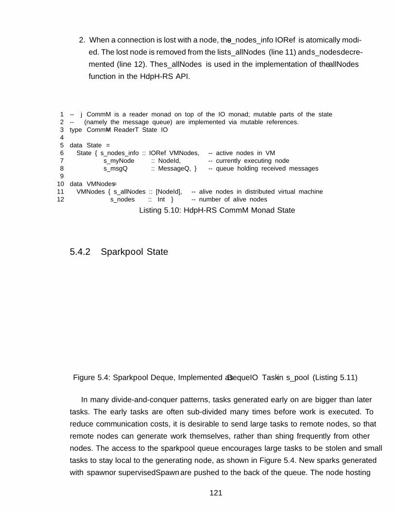
2. When a connection is lost with a node, the s_nodes_info IORef is atomically modi-fied. The lost node is removed from the list s_allNodes (line 11) and s_nodes decre-mented (line 12). The s_allNodes is used in the implementation of the allNodes

function in the HdpH-RS API.

1 -- | CommM is a reader monad on top of the IO monad; mutable parts of the state2 -- (namely the message queue) are implemented via mutable references.3 type CommM = ReaderT State IO45 data State =6 State { s_nodes_info :: IORef VMNodes, -- active nodes in VM7 s_myNode :: NodeId, -- currently executing node8 s_msgQ :: MessageQ, } -- queue holding received messages910 data VMNodes =11 VMNodes { s_allNodes :: [NodeId], -- alive nodes in distributed virtual machine12 s_nodes :: Int } -- number of alive nodes

Listing 5.10: HdpH-RS CommM Monad State

5.4.2 Sparkpool State

FISH

SCHEDULE putSpark

getSpark

0

1 2

3 4

5 6 7

1 2 3 4 5 6 7Sparkpool BackFront

Figure 5.4: Sparkpool Deque, Implemented as DequeIO Task in s_pool (Listing 5.11)

In many divide-and-conquer patterns, tasks generated early on are bigger than latertasks. The early tasks are often sub-divided many times before work is executed. Toreduce communication costs, it is desirable to send large tasks to remote nodes, so thatremote nodes can generate work themselves, rather than fishing frequently from othernodes. The access to the sparkpool queue encourages large tasks to be stolen and smalltasks to stay local to the generating node, as shown in Figure 5.4. New sparks generatedwith spawn or supervisedSpawn are pushed to the back of the queue. The node hosting

121

the sparkpool steals work from its own sparkpool from the back of the queue. A busy nodethat receives a FISH message from a thief pops a spark from the front of the sparkpooland replies with a SCHEDULE message containing that spark.

1 -- |’SparkM ’ is a reader monad sitting on top of the ’CommM’ monad2 type SparkM = ReaderT State CommM34 -- spark pool state (mutable bits held in IORefs and the like)5 data State =6 State { s_pool :: DequeIO Task, -- actual spark pool7 s_guard_post :: IORef GuardPost, -- spark suspended for authorisation8 s_sparkOrig :: IORef (Maybe NodeId), -- origin of most recent spark recvd9 s_fishing :: IORef Bool, -- True iff FISH outstanding10 s_noWork :: ActionServer } -- for clearing "FISH outstndg" flag

Listing 5.11: HdpH-RS SparkM Monad State

The SparkM monad sits on top of the CommM monad. It encapsulates the sparkpoolstate, in Listing 5.11. The sparkpool itself is s_pool on line 6. It is a double-ended queuethat contains tasks of type Task, holding both supervised and unsupervised sparks. Theguard post s_guard_post on line 7 is either empty or holds one supervised spark that isheld for an authorised migration. The fishing protocol is optimised to fish from the nodeit has most recently received a SCHEDULE message, in the hope it has more on offer. Thes_sparkOrig field holds this information on line 8. The s_fishing boolean on line 9 isused to indicate whether a node is in the process of a work stealing i.e. waiting for a replyto a FISH message. The s_noWork field corresponds to the waitingFishReplyFrom fieldin typedef WorkerNode in the Promela model (Section 4.3.3). It is reset when a NOWORK

message is received, allowing a node to fish for sparks once again.

5.4.3 Threadpool State

The ThreadM monad sits on top of the SparkM monad. It encapsulates the threadpoolstate, in Listing 5.12. In the benchmark executions in Chapter 6, the number of thread-pools matches the number of utilised cores per node. The state on line 5 is a list ofthreadpools. Each threadpool is a doubled-ended queue. Access to the threadpool is con-trolled in the same way as the sparkpool. Each scheduler accesses its own threadpoolfrom the back. Schedulers are able to steal from the front of other threadpools on thesame shared-memory node, when their own threadpool is empty.

122

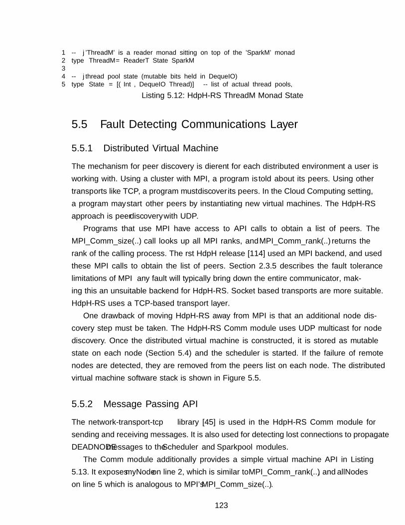
1 -- |’ThreadM’ is a reader monad sitting on top of the ’SparkM’ monad2 type ThreadM = ReaderT State SparkM34 -- |thread pool state (mutable bits held in DequeIO)5 type State = [(Int, DequeIO Thread)] -- list of actual thread pools,

Listing 5.12: HdpH-RS ThreadM Monad State

5.5 Fault Detecting Communications Layer

5.5.1 Distributed Virtual Machine

The mechanism for peer discovery is different for each distributed environment a user isworking with. Using a cluster with MPI, a program is told about its peers. Using othertransports like TCP, a program must discover its peers. In the Cloud Computing setting,a program may start other peers by instantiating new virtual machines. The HdpH-RSapproach is peer discovery with UDP.

Programs that use MPI have access to API calls to obtain a list of peers. TheMPI_Comm_size(..) call looks up all MPI ranks, and MPI_Comm_rank(..) returns therank of the calling process. The first HdpH release [114] used an MPI backend, and usedthese MPI calls to obtain the list of peers. Section 2.3.5 describes the fault tolerancelimitations of MPI — any fault will typically bring down the entire communicator, mak-ing this an unsuitable backend for HdpH-RS. Socket based transports are more suitable.HdpH-RS uses a TCP-based transport layer.

One drawback of moving HdpH-RS away from MPI is that an additional node dis-covery step must be taken. The HdpH-RS Comm module uses UDP multicast for nodediscovery. Once the distributed virtual machine is constructed, it is stored as mutablestate on each node (Section 5.4) and the scheduler is started. If the failure of remotenodes are detected, they are removed from the peers list on each node. The distributedvirtual machine software stack is shown in Figure 5.5.

5.5.2 Message Passing API

The network-transport-tcp library [45] is used in the HdpH-RS Comm module forsending and receiving messages. It is also used for detecting lost connections to propagateDEADNODE messages to the Scheduler and Sparkpool modules.

The Comm module additionally provides a simple virtual machine API in Listing5.13. It exposes myNode on line 2, which is similar to MPI_Comm_rank(..), and allNodes

on line 5 which is analogous to MPI’s MPI_Comm_size(..).

123

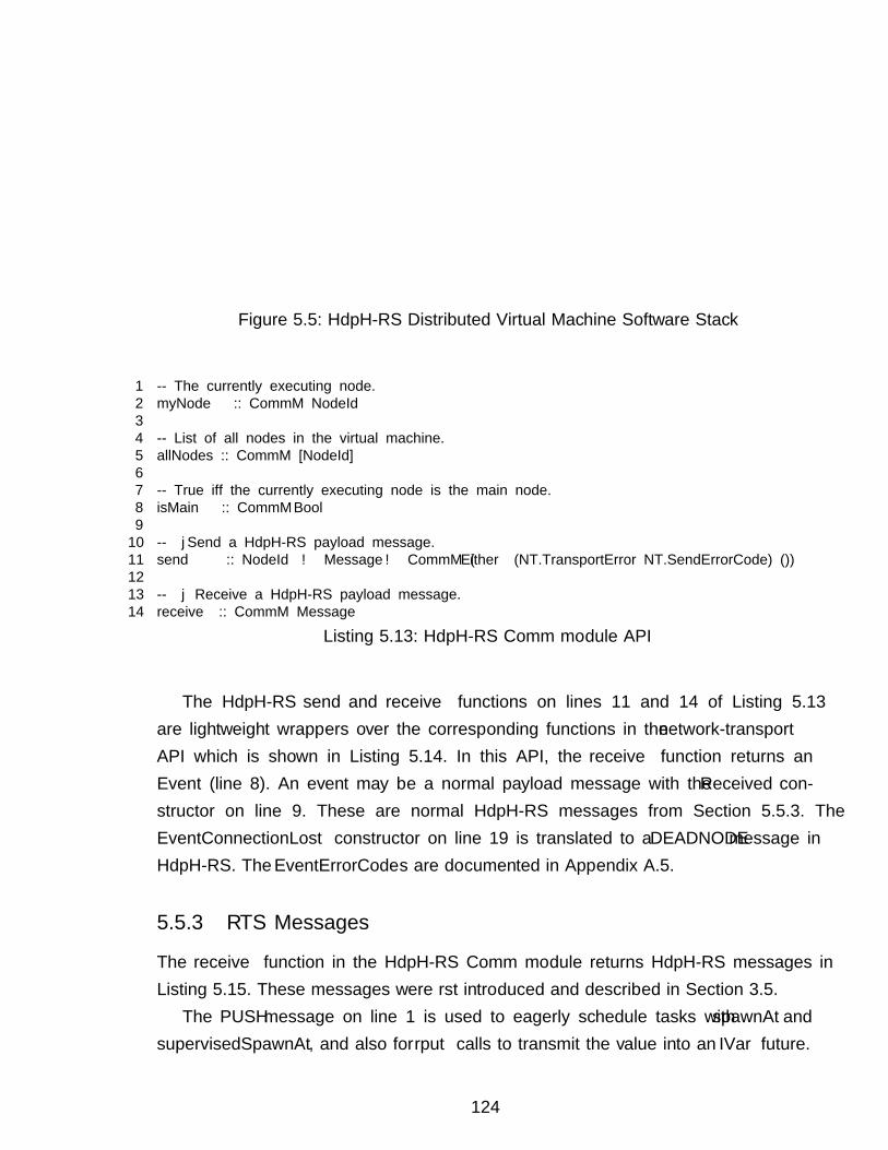
Sockets API

Ethernet

IP

TCP

Sockets API

Ethernet

IP

TCP

Sockets API

Ethernet

IP

TCP

Network−Transport API Network−Transport API Network−Transport API

Node A (root) Node CNode B

HdpH−RS API

Executable instance

Threadpools

HdpH−RS API

Executable instance

Threadpools

HdpH−RS API

Executable instance

ThreadpoolsSparkpool SparkpoolSparkpool

HdpH−RS Distributed Virtual Machine

Figure 5.5: HdpH-RS Distributed Virtual Machine Software Stack

1 -- The currently executing node.2 myNode :: CommM NodeId34 -- List of all nodes in the virtual machine.5 allNodes :: CommM [NodeId]67 -- True iff the currently executing node is the main node.8 isMain :: CommM Bool910 -- |Send a HdpH-RS payload message.11 send :: NodeId → Message → CommM (Either (NT.TransportError NT.SendErrorCode) ())1213 -- | Receive a HdpH-RS payload message.14 receive :: CommM Message

Listing 5.13: HdpH-RS Comm module API

The HdpH-RS send and receive functions on lines 11 and 14 of Listing 5.13are lightweight wrappers over the corresponding functions in the network-transport

API which is shown in Listing 5.14. In this API, the receive function returns anEvent (line 8). An event may be a normal payload message with the Received con-structor on line 9. These are normal HdpH-RS messages from Section 5.5.3. TheEventConnectionLost constructor on line 19 is translated to a DEADNODE message inHdpH-RS. The EventErrorCodes are documented in Appendix A.5.

5.5.3 RTS Messages

The receive function in the HdpH-RS Comm module returns HdpH-RS messages inListing 5.15. These messages were first introduced and described in Section 3.5.

The PUSH message on line 1 is used to eagerly schedule tasks with spawnAt andsupervisedSpawnAt, and also for rput calls to transmit the value into an IVar future.

124

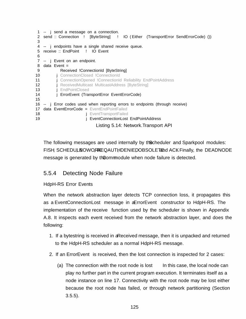
1 -- | send a message on a connection.2 send :: Connection → [ByteString] → IO (Either (TransportError SendErrorCode) ())34 -- | endpoints have a single shared receive queue.5 receive :: EndPoint → IO Event67 -- | Event on an endpoint.8 data Event =9 Received !ConnectionId [ByteString]10 | ConnectionClosed !ConnectionId11 | ConnectionOpened !ConnectionId Reliability EndPointAddress12 | ReceivedMulticast MulticastAddress [ByteString]13 | EndPointClosed14 | ErrorEvent (TransportError EventErrorCode)1516 -- | Error codes used when reporting errors to endpoints (through receive)17 data EventErrorCode = EventEndPointFailed18 | EventTransportFailed19 | EventConnectionLost EndPointAddress

Listing 5.14: Network.Transport API

The following messages are used internally by the Scheduler and Sparkpool modules:FISH, SCHEDULE, NOWORK, REQ, AUTH, DENIED, OBSOLETE and ACK. Finally, the DEADNODE

message is generated by the Comm module when node failure is detected.

5.5.4 Detecting Node Failure

HdpH-RS Error Events

When the network abstraction layer detects TCP connection loss, it propagates thisas a EventConnectionLost message in a ErrorEvent constructor to HdpH-RS. Theimplementation of the receive function used by the scheduler is shown in AppendixA.8. It inspects each event received from the network abstraction layer, and does thefollowing:

1. If a bytestring is received in a Received message, then it is unpacked and returnedto the HdpH-RS scheduler as a normal HdpH-RS message.

2. If an ErrorEvent is received, then the lost connection is inspected for 2 cases:

(a) The connection with the root node is lost In this case, the local node canplay no further part in the current program execution. It terminates itself as anode instance on line 17. Connectivity with the root node may be lost eitherbecause the root node has failed, or through network partitioning (Section3.5.5).

125

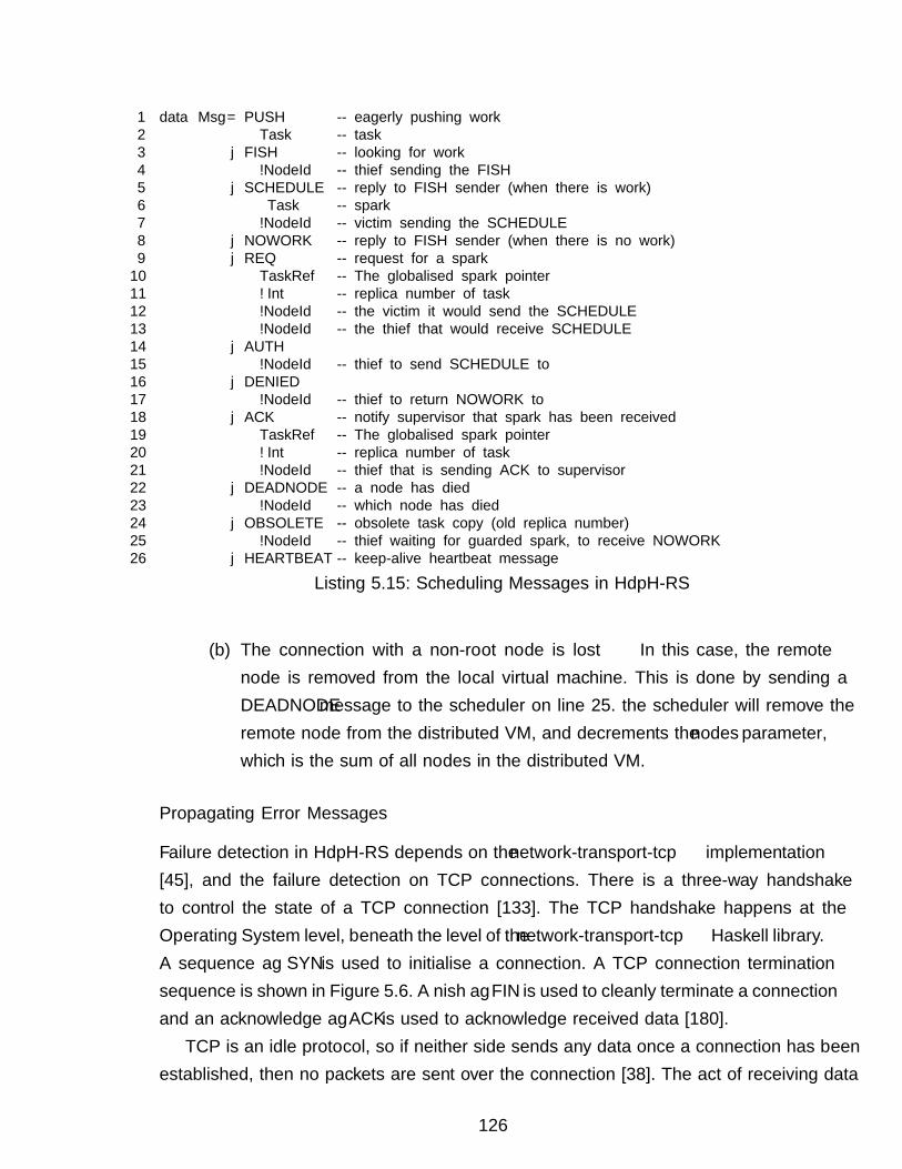
1 data Msg = PUSH -- eagerly pushing work2 Task -- task3 | FISH -- looking for work4 !NodeId -- thief sending the FISH5 | SCHEDULE -- reply to FISH sender (when there is work)6 Task -- spark7 !NodeId -- victim sending the SCHEDULE8 | NOWORK -- reply to FISH sender (when there is no work)9 | REQ -- request for a spark10 TaskRef -- The globalised spark pointer11 !Int -- replica number of task12 !NodeId -- the victim it would send the SCHEDULE13 !NodeId -- the thief that would receive SCHEDULE14 | AUTH15 !NodeId -- thief to send SCHEDULE to16 | DENIED17 !NodeId -- thief to return NOWORK to18 | ACK -- notify supervisor that spark has been received19 TaskRef -- The globalised spark pointer20 !Int -- replica number of task21 !NodeId -- thief that is sending ACK to supervisor22 | DEADNODE -- a node has died23 !NodeId -- which node has died24 | OBSOLETE -- obsolete task copy (old replica number)25 !NodeId -- thief waiting for guarded spark, to receive NOWORK26 | HEARTBEAT -- keep-alive heartbeat message

Listing 5.15: Scheduling Messages in HdpH-RS

(b) The connection with a non-root node is lost In this case, the remotenode is removed from the local virtual machine. This is done by sending aDEADNODE message to the scheduler on line 25. the scheduler will remove theremote node from the distributed VM, and decrements the nodes parameter,which is the sum of all nodes in the distributed VM.

Propagating Error Messages

Failure detection in HdpH-RS depends on the network-transport-tcp implementation[45], and the failure detection on TCP connections. There is a three-way handshaketo control the state of a TCP connection [133]. The TCP handshake happens at theOperating System level, beneath the level of the network-transport-tcp Haskell library.A sequence flag SYN is used to initialise a connection. A TCP connection terminationsequence is shown in Figure 5.6. A finish flag FIN is used to cleanly terminate a connectionand an acknowledge flag ACK is used to acknowledge received data [180].

TCP is an idle protocol, so if neither side sends any data once a connection has beenestablished, then no packets are sent over the connection [38]. The act of receiving data

126

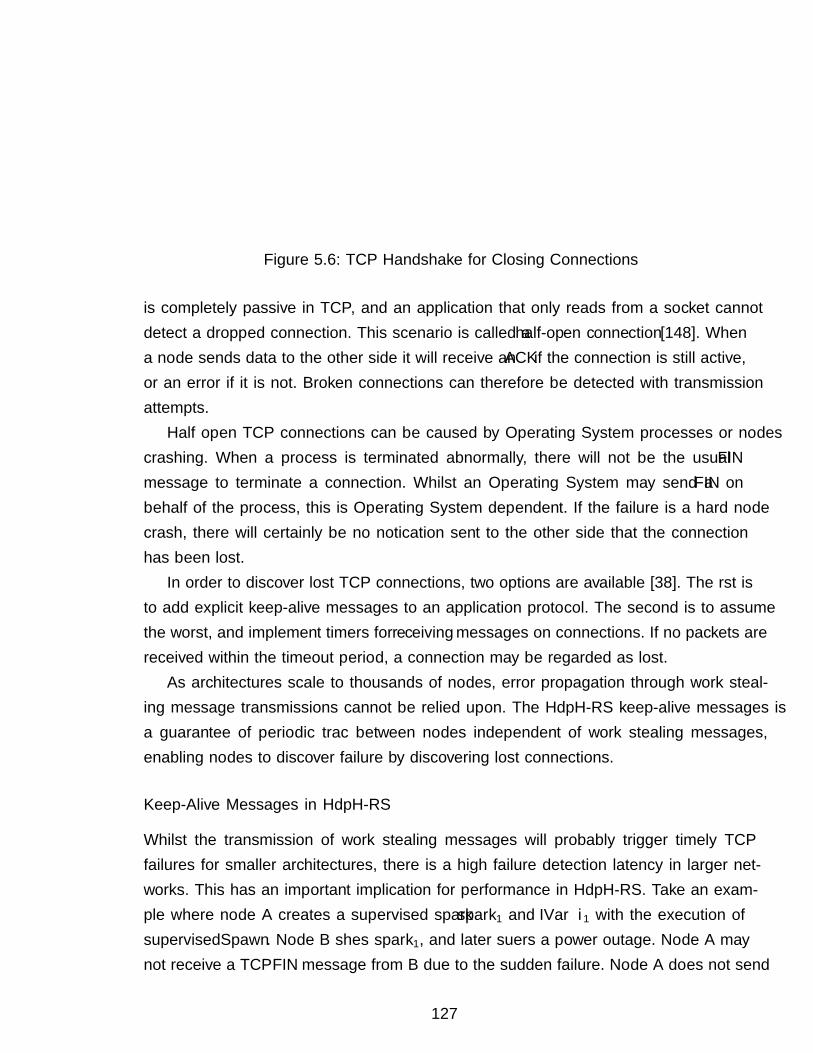
Established

connection

Established

connection

active close

Closed

TIME_WAIT

FIN_WAIT_2

FIN_WAIT_1 FIN

ACK

FIN

ACK

Initiator Receiver

Closed

passive closeCLOSE_WAIT

LAST_ACK

Figure 5.6: TCP Handshake for Closing Connections

is completely passive in TCP, and an application that only reads from a socket cannotdetect a dropped connection. This scenario is called a half-open connection [148]. Whena node sends data to the other side it will receive an ACK if the connection is still active,or an error if it is not. Broken connections can therefore be detected with transmissionattempts.

Half open TCP connections can be caused by Operating System processes or nodescrashing. When a process is terminated abnormally, there will not be the usual FINmessage to terminate a connection. Whilst an Operating System may send a FIN onbehalf of the process, this is Operating System dependent. If the failure is a hard nodecrash, there will certainly be no notification sent to the other side that the connectionhas been lost.

In order to discover lost TCP connections, two options are available [38]. The first isto add explicit keep-alive messages to an application protocol. The second is to assumethe worst, and implement timers for receiving messages on connections. If no packets arereceived within the timeout period, a connection may be regarded as lost.

As architectures scale to thousands of nodes, error propagation through work steal-ing message transmissions cannot be relied upon. The HdpH-RS keep-alive messages isa guarantee of periodic traffic between nodes independent of work stealing messages,enabling nodes to discover failure by discovering lost connections.

Keep-Alive Messages in HdpH-RS

Whilst the transmission of work stealing messages will probably trigger timely TCPfailures for smaller architectures, there is a high failure detection latency in larger net-works. This has an important implication for performance in HdpH-RS. Take an exam-ple where node A creates a supervised spark spark1 and IVar i1 with the execution ofsupervisedSpawn. Node B fishes spark1, and later suffers a power outage. Node A maynot receive a TCP FIN message from B due to the sudden failure. Node A does not send

127

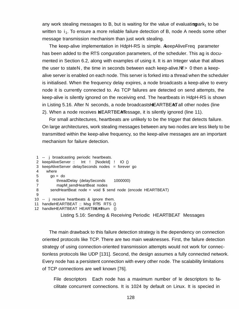
any work stealing messages to B, but is waiting for the value of evaluating spark1 to bewritten to i1. To ensure a more reliable failure detection of B, node A needs some othermessage transmission mechanism than just work stealing.

The keep-alive implementation in HdpH-RS is simple. A keepAliveFreq parameterhas been added to the RTS configuration parameters, of the scheduler. This flag is docu-mented in Section 6.2, along with examples of using it. It is an Integer value that allowsthe user to state N , the time in seconds between each keep-alive. If N > 0 then a keep-alive server is enabled on each node. This server is forked into a thread when the scheduleris initialised. When the frequency delay expires, a node broadcasts a keep-alive to everynode it is currently connected to. As TCP failures are detected on send attempts, thekeep-alive is silently ignored on the receiving end. The heartbeats in HdpH-RS is shownin Listing 5.16. After N seconds, a node broadcasts a HEARTBEAT to all other nodes (line2). When a node receives a HEARTBEAT message, it is silently ignored (line 11).

For small architectures, heartbeats are unlikely to be the trigger that detects failure.On large architectures, work stealing messages between any two nodes are less likely to betransmitted within the keep-alive frequency, so the keep-alive messages are an importantmechanism for failure detection.

1 -- | broadcasting periodic heartbeats.2 keepAliveServer :: Int → [NodeId] → IO ()3 keepAliveServer delaySeconds nodes = forever go4 where5 go = do6 threadDelay (delaySeconds ∗ 1000000)7 mapM_ sendHeartBeat nodes8 sendHeartBeat node = void $ send node (encode HEARTBEAT)910 -- | receive heartbeats & ignore them.11 handleHEARTBEAT :: Msg RTS → RTS ()12 handleHEARTBEAT HEARTBEAT = return ()

Listing 5.16: Sending & Receiving Periodic HEARTBEAT Messages

The main drawback to this failure detection strategy is the dependency on connectionoriented protocols like TCP. There are two main weaknesses. First, the failure detectionstrategy of using connection-oriented transmission attempts would not work for connec-tionless protocols like UDP [131]. Second, the design assumes a fully connected network.Every node has a persistent connection with every other node. The scalability limitationsof TCP connections are well known [76].

• File descriptors Each node has a maximum number of file descriptors to fa-cilitate concurrent connections. It is 1024 by default on Linux. It is specified in

128

/proc/sys/fs/file-max, though can easily be changed.

• Socket buffers Each TCP connection contain a socket receive and send buffer. Areceive buffer may be in the 87kb region (in file /proc/sys/net/ipv4/tcp_rmem)and write buffers in the 16kb region (in file /proc/sys/net/ipv4/tcp_wmem). AnOperating System allocates memory for socket buffers, which limits the number oftheoretically possible TCP connections.

The author is in discussion [88] with the network-transport authors on a generalisedfailure detection for distributed Haskells. A failure detection mechanism has not yetbeen added to the library. The proposed generalised strategy is to use passive heartbeattimeouts. That is, every node broadcasts a timeout, and expects a heartbeat messagefrom all other nodes. If a heartbeat is not received from a remote node within a giventimeout threshold, it is assumed to have failed. It is the opposite to HdpH-RS, whichdetects failure actively on the heartbeat broadcaster, not passively on the receiver.

The generalised fault detection design for distributed Haskells does have some draw-backs. First, network congestion may delay message delivery that results in false-positivesin failure detection [191]. Second, the latency of failure detection is higher. It is at leastthe size of the timeout window + the delay between heartbeats (Section 2.2.3).

5.6 Comparison with Other Fault Tolerant LanguageImplementations

The implementation of fault tolerance in HdpH-RS shares many techniques with otherfault tolerant programming languages and distributed schedulers. Replication (Section2.2.3) is the key recovery mechanism in HdpH-RS. It is a tactic used in the supervisionbehaviours of Erlang [7], and is ingrained in the Google MapReduce model [49], such asin Hadoop [183].

5.6.1 Erlang

The supervision approach in Erlang is a strong influence on the implementation of HdpH-RS. Below are four distinctions between the performance of Erlang and HdpH in theabsence of faults, and the recovery in Erlang and HdpH-RS in the presence of faults.

Handling failures The failure recovery in HdpH-RS is akin to the Erlang OTP super-vision behaviours. The user does not need to handle failures programmatically. However,when the monitor and link Erlang primitives are used directly, it is the responsibilityof the programmer to recover from faults.

129

Recovering stateful computations Erlang has better support for recovering non-idempotent computations, using the restart strategies and frequencies of the supervisionbehaviour in Erlang OTP. HdpH-RS does not support the recovery of non-idempotenttasks, and is designed for evaluating pure expressions that are of course idempotent.

Load balancing Support for load balancing is more powerful in HdpH and HdpH-RSthan in Erlang. A work stealing mechanism in Erlang could be thought of as HdpH-RSwithout sparkpools and only threadpools — once an Erlang process is spawned, it cannotmigrate to another node. This makes Erlang less suitable than HdpH-RS for some classesof computation, where parallelism is highly irregular. Parallel symbolic computing is oneexample.

Programming errors Erlang is an untyped language, allowing many programmingerrors to go unnoticed at compile time [174]. Such typing error can introduce faults atruntime. A type system has been proposed [119], though is not often used. Only a subsetof the language is type-checkable, the major omission being the lack of process types [6].In contrast, the Haskell host language for HdpH-RS is strongly typed, eliminating a largeclass of software bugs at compile time.

5.6.2 Hadoop

Hadoop is a popular MapReduce implementation. MapReduce is a programming modeland an associated implementation for processing and generating large data sets [49]. IfHadoop is used using the MapReduce interface directly, a programmer only defines amap and a reduce function, and these are automatically parallelisable.

To relate the programming model to HdpH-RS, the MapReduce model is in factan algorithmic skeleton. It has been implemented in HdpH-RS as 2 of 10 parallelskeletons. First an implicit parMapReduceRangeThresh skeleton, and second an explicitpushMapReduceRangeThresh skeleton. They are used in the implementation of the Man-delbrot benchmark in Section 6.3.1. The failure recovery in Hadoop is task replication,the same as Erlang and HdpH-RS. The failure recovery in HdpH-RS can be compared toHadoop in three ways:

Failure detection latency Failure detection latency in Hadoop is 10 minutes bydefault in order to tolerate non-responsiveness and network congestion. A slave sends aheartbeat to the master node every 3 seconds. If the master does not receive a heartbeatfrom a given slave within a 10 minute window, failure is assumed [55]. In contrast, thefailure detection latency in HdpH-RS is a maximum of 5 seconds by default, and can bemodified by the user.

Supervision Bottleneck A master node supervises the health of all slave nodes

130

in Hadoop. In contrast, the HdpH-RS architecture supports hierarchically nested super-visors. This is achieved with either recursive supervisedSpawn or supervisedSpawnAtcalls, or by using the MapReduce or divide-and-conquer skeletons. This means that super-vision and task replication responsibilities are distributed across the entire architecturein HdpH-RS, and not centrally coordinated like Hadoop.

Unnecessary task replication The output of map tasks are stored to disk locally inHadoop. In the presence of failure, completed map tasks are re-scheduled, due to the lossof their results. This is in contrast to HdpH-RS, where the resulting values of evaluatingtask expressions is transmitted with rput as soon as they are calculated.

5.6.3 GdH Fault Tolerance Design

The design of a new RTS level of fault tolerance for Glasgow distributed Haskell (GdH)[173] has been proposed, but not implemented. The design augments the GdH RTS witherror detection and error recovery.

The failure detection is similar to the HdpH-RS detection. It is designed to relyon the eager node failure detection from its PVM [15] network layer. As in HdpH-RS, intermittent node failure is managed by ignoring future message from the faultynode. When the transport layer broadcasts the node failure, future messages sent by apreviously faulty node are discarded — by the scheduler in the case of GdH, and bynetwork-transport-tcp [45] library in the case of HdpH-RS.

Simultaneous failure recovery in the GdH design is similar to the HdpH-RS implemen-tation. In both, one node is distinguished as the root node, which starts and terminatesthe program. If a network is split in to two or more parts, the partition containing theroot node will restart the pure computations from the lost partitions.

In order to replicate pure computations in the presence of failure, both the GdHdesign and HdpH-RS store task copies on the creating node. The store of these tasks isdefined as a backup heap in GdH. The back-up task copies in HdpH-RS are stored withintheir corresponding empty future.

The GdH fault tolerance design include some techniques borrowed from Erlang, thathave not been adopted in HdpH-RS. One example is continued service. A computationcannot be restarted more than a fixed number of times before raising an exception inthe GdH design, similar to the child process restart frequency in Erlang OTP. A messageis not re-transmitted more than a fixed number of times before raising an exception,preventing livelock. Finally, nodes can be added during the execution of programs, toreplace failed nodes. None of these 3 features have been implemented in HdpH-RS.

131

5.6.4 Fault Tolerant MPI Implementations

Most scientific applications are written in C with MPI [98]. The original MPI standardsspecify very limited features related to reliability and fault tolerance [73]. Based on earlyMPI standards, an entire application is shutdown when one of the executing processorsexperiences a failure. As discussed in Section 2.3.5, MPI implementations that includefault tolerant take one of two approaches. Either they hide faults from the user, or propa-gate them for the user to recover from faults programmatically. Some fault tolerant MPIimplementations mask faults, but thereafter support a reduced set of MPI operations.This masking of failures is the same approach as HdpH-RS, with the difference that noprogramming primitives are disabled by faults.

132

Chapter 6

Fault Tolerant Programming &Reliable Scheduling Evaluation

This chapter demonstrates how to program with reliable scheduling and gives a per-formance evaluation of HdpH-RS. Section 6.1.1 demonstrates how to write fault tol-erance programs with HdpH-RS. The parallel skeletons from HdpH have been portedto HdpH-RS (Section 6.1.2), adding fault tolerance by implementing them using thesupervisedSpawn and supervisedSpawnAt primitives. Section 6.2 describes how tolaunch HdpH-RS programs on clustered architectures, and how to configure the HdpH-RSRTS for fault tolerance and performance tuning. Section 6.3.1 describes the five bench-marks used to evaluate HdpH-RS. Section 6.3.3 describes the two architectures on whichHdpH-RS has been measured. One is a 32 node Beowulf cluster providing 224 cores. Theother is HECToR, a high performance UK national compute resource, and up to 1400cores are used to measure the scalability of HdpH-RS.

The supervision overheads of the fault tolerant work stealing protocol (Section 3.5)are compared against the HdpH fault oblivious scheduling in Section 6.4, by measur-ing the fault tolerant and non-fault tolerant version of three skeletons — parallel-map,divide-and-conquer and map-reduce. The benchmark executions demonstrate the scala-bility of fault tolerance in HdpH-RS. For example, the Summatory Liouville benchmarkdemonstrates HdpH-RS speedup of 145 on 224 cores on Beowulf, and a speedup of 751on 1400 cores on HECToR. The recovery overheads of detecting faults and replicatingtasks is measured in Section 6.5 by injecting two types of failure during execution usingthe HdpH-RS scheduler. The first type simulates simultaneous node loss (Section 6.5.1),which can occur when networks are partitioned. The second type uses a Chaos Monkeyimplementation in HdpH-RS (Section 6.5.2), to simulate random failure. Unit tests areused ensure that programs using the fault tolerant skeletons terminate with the correct

133

result in the presence of Chaos Monkey failure injection. The runtime performance ofHdpH-RS indicate that lazy on-demand work stealing is more suitable when failure isthe common case, not the exception.

6.1 Fault Tolerant Programming with HdpH-RS

This section shows how to program with HdpH-RS primitives and skeletons. The use caseis a parallel implementation of Euler’s totient function φ [102]. It is an arithmetic functionthat counts the totatives of n, i.e. the positive integers less than or equal to n that arerelatively prime to n. Listing 6.1 shows the implementation of φ and the sequential sumof totients. It is parallelised in Section 6.1.1 using the HdpH-RS primitives directly, andin Section 6.1.3 using the parMapSlicedFT skeleton.

1 -- | Euler’s totient function (for positive integers)2 totient :: Int → Integer3 totient n = toInteger $ length $ filter (λ k → gcd n k == 1) [1..n]45 -- | sequential sum of totients6 sum_totient :: [Int] → Integer7 sum_totient = sum ◦ map totient

Listing 6.1: Sequential Implementation of Sum Euler

6.1.1 Programming With HdpH-RS Fault Tolerance Primitives

Using the HdpH-RS primitives directly for computing Sum Euler between 0 and 10000with a slice size of 100 is shown in Listing 6.2. The dist_sum_totient_sliced functioncreates a sliced list of lists on line 5 using the lower and upper bounds and chunk size.For each element in the list, a supervised spark and corresponding IVar (the supervisedfuture) is created with supervisedSpawn on line 11. The results are summed on line 3.The main function on line 16 prints the result 30397486.

6.1.2 Fault Tolerant Parallel Skeletons

Algorithmic skeletons abstract commonly-used patterns of parallel computation, commu-nication, and interaction [39]. The implementation of skeletons manage logic, arithmeticand control flow operations, communication and data exchange, task creation, and syn-chronisation. Skeletons provide a top-down design approach, and are often compositional[71].

134

1 dist_sum_totient_sliced :: Int → Int → Int → Par Integer2 dist_sum_totient_sliced lower upper chunksize = do3 sum <$> (mapM get_and_unClosure =« (mapM spawn_sum_euler $ sliced_list))4 where5 sliced_list = slice slices [upper, upper - 1 .. lower] :: [[Int]]67 get_and_unClosure :: IVar (Closure a) → Par a8 get_and_unClosure = return ◦ unClosure <=< get910 spawn_sum_euler :: [Int] → Par (IVar (Closure Integer))11 spawn_sum_euler xs = supervisedSpawn $(mkClosure [ | spawn_sum_euler_abs (xs) |])1213 spawn_sum_euler_abs :: ([Int]) → Par (Closure Integer)14 spawn_sum_euler_abs (xs) = force (sum_totient xs) »= return ◦ toClosure1516 main = do17 result ← runParIO conf (dist_sum_totient_sliced0 10000 100)18 print result -- "30397486"

Listing 6.2: Programming with HdpH-RS Primitives Directly

The supervisedSpawn and supervisedSpawnAt primitives from Section 3.3.2 guar-antee the evaluation of a single task — a supervised spark or thread corresponding toa supervised future. Higher-level abstractions built on top of these primitives guaranteethe completion of a set of tasks of this type. These abstractions hide lower level detailsby creating supervised sparks or threads, and supervised futures (IVars) dynamically.

Eight parallel skeletons from HdpH have been extended for fault tolerance. HdpH-RS introduces four skeleton patterns to the HdpH skeletons library: parMapForkM,forkDivideAndConquer, parMapReduceRangeThresh and pushMapReduceRangeThresh.The first two abstract shared-memory parallel patterns, and the latter two are extendedfor fault tolerance as parMapReduceRangeThreshFT and pushMapReduceRangeThreshFT.The HdpH-RS skeletons API is in Appendix A.9. Lazy work stealing skeletons are re-placed with supervised lazy work stealing versions by using supervisedSpawn. Fault tol-erant skeletons that use eager task placement are implemented with supervisedSpawnAt.As an example, Listing 6.3 shows the implementation of the fault tolerant parallel-mapskeleton parMapFT. It uses a parClosureList strategy on line 12 which uses the faulttolerant HdpH-RS supervisedSpawn primitive within sparkClosure on line 17. Thereare variants of parallel-map skeletons, for slicing and chunking input lists.

Divide-and-conquer is a more elaborate recursive parallel pattern. A fault tolerantparDivideAndConquerFT skeleton is shown in Listing 6.4. It is a skeleton that allows aproblem to be decomposed into sub-problems until they are sufficiently small, and thenreassembled with a combining function. Its use is demonstrated with Queens in Section

135

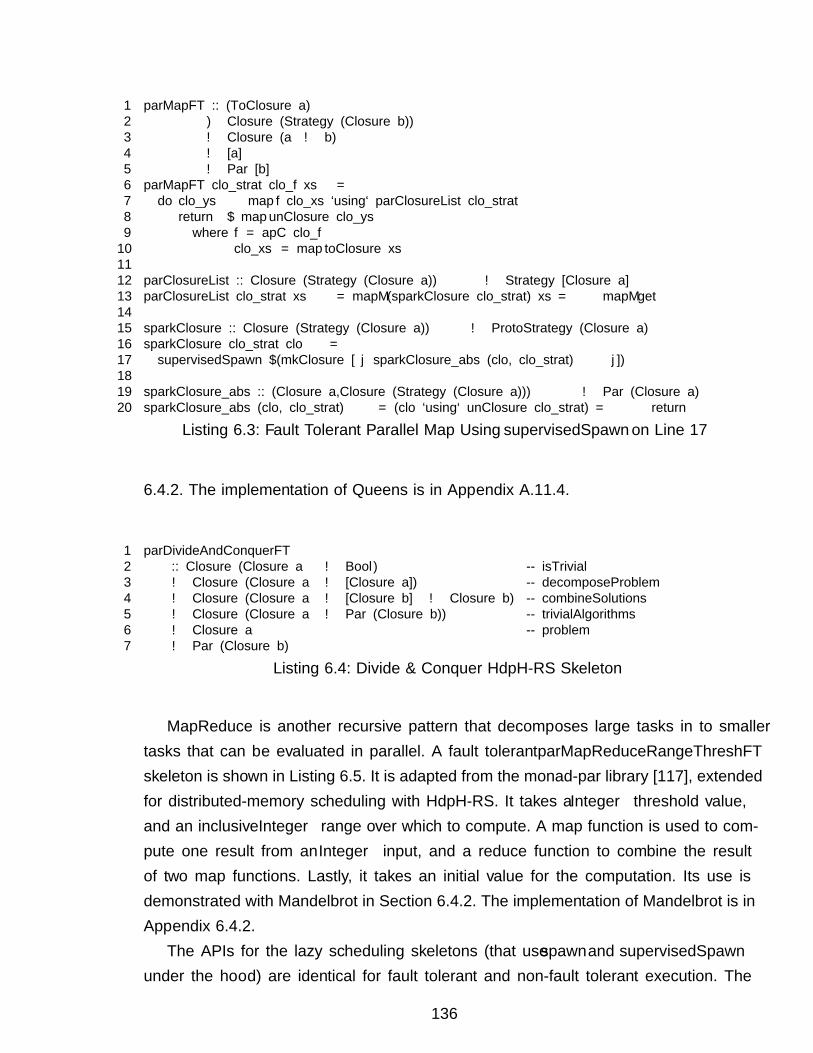
1 parMapFT :: (ToClosure a)2 ⇒ Closure (Strategy (Closure b))3 → Closure (a → b)4 → [a]5 → Par [b]6 parMapFT clo_strat clo_f xs =7 do clo_ys ← map f clo_xs ‘using‘ parClosureList clo_strat8 return $ map unClosure clo_ys9 where f = apC clo_f10 clo_xs = map toClosure xs1112 parClosureList :: Closure (Strategy (Closure a)) → Strategy [Closure a]13 parClosureList clo_strat xs = mapM (sparkClosure clo_strat) xs »= mapM get1415 sparkClosure :: Closure (Strategy (Closure a)) → ProtoStrategy (Closure a)16 sparkClosure clo_strat clo =17 supervisedSpawn $(mkClosure [ | sparkClosure_abs (clo, clo_strat) |])1819 sparkClosure_abs :: (Closure a,Closure (Strategy (Closure a))) → Par (Closure a)20 sparkClosure_abs (clo, clo_strat) = (clo ‘using‘ unClosure clo_strat) »= return

Listing 6.3: Fault Tolerant Parallel Map Using supervisedSpawn on Line 17

6.4.2. The implementation of Queens is in Appendix A.11.4.

1 parDivideAndConquerFT2 :: Closure (Closure a → Bool) -- isTrivial3 → Closure (Closure a → [Closure a]) -- decomposeProblem4 → Closure (Closure a → [Closure b] → Closure b) -- combineSolutions5 → Closure (Closure a → Par (Closure b)) -- trivialAlgorithms6 → Closure a -- problem7 → Par (Closure b)

Listing 6.4: Divide & Conquer HdpH-RS Skeleton

MapReduce is another recursive pattern that decomposes large tasks in to smallertasks that can be evaluated in parallel. A fault tolerant parMapReduceRangeThreshFT

skeleton is shown in Listing 6.5. It is adapted from the monad-par library [117], extendedfor distributed-memory scheduling with HdpH-RS. It takes a Integer threshold value,and an inclusive Integer range over which to compute. A map function is used to com-pute one result from an Integer input, and a reduce function to combine the resultof two map functions. Lastly, it takes an initial value for the computation. Its use isdemonstrated with Mandelbrot in Section 6.4.2. The implementation of Mandelbrot is inAppendix 6.4.2.

The APIs for the lazy scheduling skeletons (that use spawn and supervisedSpawn

under the hood) are identical for fault tolerant and non-fault tolerant execution. The

136

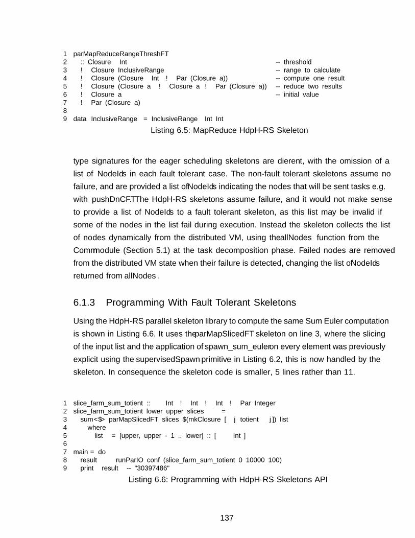
1 parMapReduceRangeThreshFT2 :: Closure Int -- threshold3 → Closure InclusiveRange -- range to calculate4 → Closure (Closure Int → Par (Closure a)) -- compute one result5 → Closure (Closure a → Closure a → Par (Closure a)) -- reduce two results6 → Closure a -- initial value7 → Par (Closure a)89 data InclusiveRange = InclusiveRange Int Int

Listing 6.5: MapReduce HdpH-RS Skeleton

type signatures for the eager scheduling skeletons are different, with the omission of alist of NodeIds in each fault tolerant case. The non-fault tolerant skeletons assume nofailure, and are provided a list of NodeIds indicating the nodes that will be sent tasks e.g.with pushDnCFT. The HdpH-RS skeletons assume failure, and it would not make senseto provide a list of NodeIds to a fault tolerant skeleton, as this list may be invalid ifsome of the nodes in the list fail during execution. Instead the skeleton collects the listof nodes dynamically from the distributed VM, using the allNodes function from theComm module (Section 5.1) at the task decomposition phase. Failed nodes are removedfrom the distributed VM state when their failure is detected, changing the list of NodeIdsreturned from allNodes.

6.1.3 Programming With Fault Tolerant Skeletons

Using the HdpH-RS parallel skeleton library to compute the same Sum Euler computationis shown in Listing 6.6. It uses the parMapSlicedFT skeleton on line 3, where the slicingof the input list and the application of spawn_sum_euler on every element was previouslyexplicit using the supervisedSpawn primitive in Listing 6.2, this is now handled by theskeleton. In consequence the skeleton code is smaller, 5 lines rather than 11.

1 slice_farm_sum_totient :: Int → Int → Int → Par Integer2 slice_farm_sum_totient lower upper slices =3 sum <$> parMapSlicedFT slices $(mkClosure [ | totient |]) list4 where5 list = [upper, upper - 1 .. lower] :: [Int]67 main = do8 result ← runParIO conf (slice_farm_sum_totient 0 10000 100)9 print result -- "30397486"

Listing 6.6: Programming with HdpH-RS Skeletons API

137

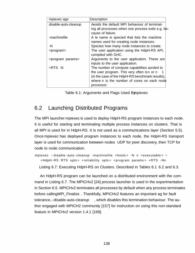
mpiexec flags Description–disable-auto-cleanup Avoids the default MPI behaviour of terminat-

ing all processes when one process exits e.g. be-cause of failure.

-machinefile A file name is specified that lists the machinenames used for creating node instances.

-N Specifies how many node instances to create.<program> The user application using the HdpH-RS API,

compiled with GHC.<program params> Arguments to the user application. These are

inputs to the user application.+RTS -N The number of compute capabilities afforded to

the user program. This very often is n or n− 1(in the case of the HdpH-RS benchmark results),where n is the number of cores on each nodeprocessor.

Table 6.1: Arguments and Flags Used By mpiexec

6.2 Launching Distributed Programs

The MPI launcher mpiexec is used to deploy HdpH-RS program instances to each node.It is useful for starting and terminating multiple process instances on clusters. That isall MPI is used for in HdpH-RS. It is not used as a communications layer (Section 5.5).Once mpiexec has deployed program instances to each node, the HdpH-RS transportlayer is used for communication between nodes — UDP for peer discovery, then TCP fornode to node communication.

mpiexec --disable -auto -cleanup -machinefile <hosts > -N n <executable > \

<HdpH -RS RTS opts > <reliability opts > <program params > +RTS -Nn

Listing 6.7: Executing HdpH-RS on Clusters. Described in Tables 6.1 6.2 and 6.3.

An HdpH-RS program can be launched on a distributed environment with the com-mand in Listing 6.7. The MPICHv2 [24] process launcher is used in the experimentationin Section 6.5. MPICHv2 terminates all processes by default when any process terminatesbefore calling MPI_Finalize. Thankfully, MPICHv2 features an important flag for faulttolerance, --disable-auto-cleanup, which disables this termination behaviour. The au-thor engaged with MPICH2 community [157] for instruction on using this non-standardfeature in MPICHv2 version 1.4.1 [169].

138

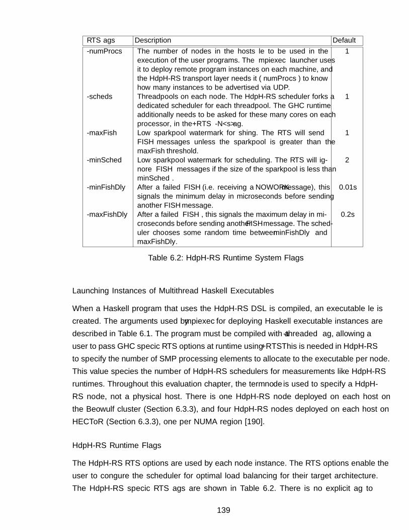
RTS flags Description Default-numProcs The number of nodes in the hosts file to be used in the

execution of the user programs. The mpiexec launcher usesit to deploy remote program instances on each machine, andthe HdpH-RS transport layer needs it ( numProcs ) to knowhow many instances to be advertised via UDP.

1

-scheds Threadpools on each node. The HdpH-RS scheduler forks adedicated scheduler for each threadpool. The GHC runtimeadditionally needs to be asked for these many cores on eachprocessor, in the +RTS -N<s> flag.

1

-maxFish Low sparkpool watermark for fishing. The RTS will sendFISH messages unless the sparkpool is greater than themaxFish threshold.

1

-minSched Low sparkpool watermark for scheduling. The RTS will ig-nore FISH messages if the size of the sparkpool is less thanminSched .

2

-minFishDly After a failed FISH (i.e. receiving a NOWORK message), thissignals the minimum delay in microseconds before sendinganother FISH message.

0.01s

-maxFishDly After a failed FISH , this signals the maximum delay in mi-croseconds before sending another FISH message. The sched-uler chooses some random time between minFishDly andmaxFishDly.

0.2s

Table 6.2: HdpH-RS Runtime System Flags

Launching Instances of Multithread Haskell Executables

When a Haskell program that uses the HdpH-RS DSL is compiled, an executable file iscreated. The arguments used by mpiexec for deploying Haskell executable instances aredescribed in Table 6.1. The program must be compiled with a -threaded flag, allowing auser to pass GHC specific RTS options at runtime using +RTS. This is needed in HdpH-RSto specify the number of SMP processing elements to allocate to the executable per node.This value specifies the number of HdpH-RS schedulers for measurements like HdpH-RSruntimes. Throughout this evaluation chapter, the term node is used to specify a HdpH-RS node, not a physical host. There is one HdpH-RS node deployed on each host onthe Beowulf cluster (Section 6.3.3), and four HdpH-RS nodes deployed on each host onHECToR (Section 6.3.3), one per NUMA region [190].

HdpH-RS Runtime Flags

The HdpH-RS RTS options are used by each node instance. The RTS options enable theuser to configure the scheduler for optimal load balancing for their target architecture.The HdpH-RS specific RTS flags are shown in Table 6.2. There is no explicit flag to

139

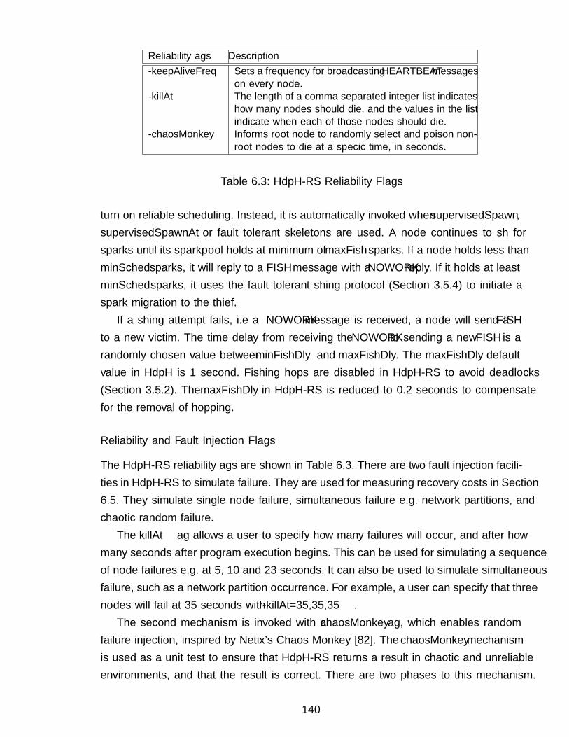
Reliability flags Description-keepAliveFreq Sets a frequency for broadcasting HEARTBEAT messages

on every node.-killAt The length of a comma separated integer list indicates

how many nodes should die, and the values in the listindicate when each of those nodes should die.

-chaosMonkey Informs root node to randomly select and poison non-root nodes to die at a specific time, in seconds.

Table 6.3: HdpH-RS Reliability Flags

turn on reliable scheduling. Instead, it is automatically invoked when supervisedSpawn,supervisedSpawnAt or fault tolerant skeletons are used. A node continues to fish forsparks until its sparkpool holds at minimum of maxFish sparks. If a node holds less thanminSched sparks, it will reply to a FISH message with a NOWORK reply. If it holds at leastminSched sparks, it uses the fault tolerant fishing protocol (Section 3.5.4) to initiate aspark migration to the thief.

If a fishing attempt fails, i.e a NOWORK message is received, a node will send a FISH

to a new victim. The time delay from receiving the NOWORK to sending a new FISH is arandomly chosen value between minFishDly and maxFishDly. The maxFishDly defaultvalue in HdpH is 1 second. Fishing hops are disabled in HdpH-RS to avoid deadlocks(Section 3.5.2). The maxFishDly in HdpH-RS is reduced to 0.2 seconds to compensatefor the removal of hopping.

Reliability and Fault Injection Flags

The HdpH-RS reliability flags are shown in Table 6.3. There are two fault injection facili-ties in HdpH-RS to simulate failure. They are used for measuring recovery costs in Section6.5. They simulate single node failure, simultaneous failure e.g. network partitions, andchaotic random failure.

The killAt flag allows a user to specify how many failures will occur, and after howmany seconds after program execution begins. This can be used for simulating a sequenceof node failures e.g. at 5, 10 and 23 seconds. It can also be used to simulate simultaneousfailure, such as a network partition occurrence. For example, a user can specify that threenodes will fail at 35 seconds with -killAt=35,35,35.

The second mechanism is invoked with a chaosMonkey flag, which enables randomfailure injection, inspired by Netflix’s Chaos Monkey [82]. The chaosMonkey mechanismis used as a unit test to ensure that HdpH-RS returns a result in chaotic and unreliableenvironments, and that the result is correct. There are two phases to this mechanism.

140

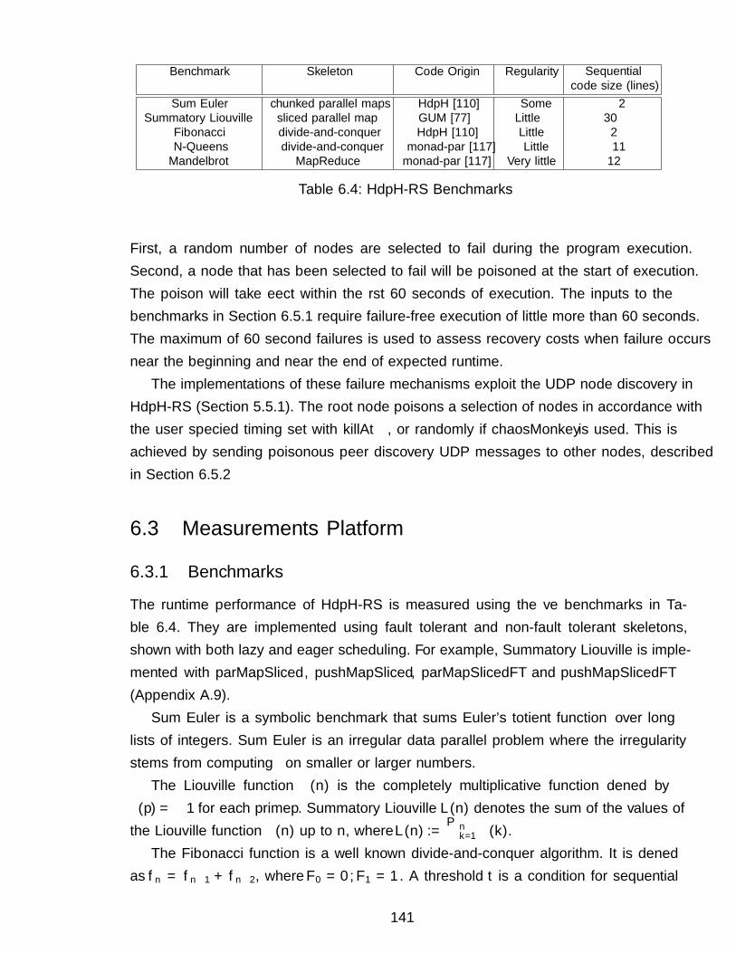
Benchmark Skeleton Code Origin Regularity Sequentialcode size (lines)

Sum Euler chunked parallel maps HdpH [110] Some 2Summatory Liouville sliced parallel map GUM [77] Little 30

Fibonacci divide-and-conquer HdpH [110] Little 2N-Queens divide-and-conquer monad-par [117] Little 11Mandelbrot MapReduce monad-par [117] Very little 12

Table 6.4: HdpH-RS Benchmarks

First, a random number of nodes are selected to fail during the program execution.Second, a node that has been selected to fail will be poisoned at the start of execution.The poison will take effect within the first 60 seconds of execution. The inputs to thebenchmarks in Section 6.5.1 require failure-free execution of little more than 60 seconds.The maximum of 60 second failures is used to assess recovery costs when failure occursnear the beginning and near the end of expected runtime.

The implementations of these failure mechanisms exploit the UDP node discovery inHdpH-RS (Section 5.5.1). The root node poisons a selection of nodes in accordance withthe user specified timing set with killAt, or randomly if chaosMonkey is used. This isachieved by sending poisonous peer discovery UDP messages to other nodes, describedin Section 6.5.2

6.3 Measurements Platform

6.3.1 Benchmarks

The runtime performance of HdpH-RS is measured using the five benchmarks in Ta-ble 6.4. They are implemented using fault tolerant and non-fault tolerant skeletons,shown with both lazy and eager scheduling. For example, Summatory Liouville is imple-mented with parMapSliced, pushMapSliced, parMapSlicedFT and pushMapSlicedFT

(Appendix A.9).Sum Euler is a symbolic benchmark that sums Euler’s totient function φ over long

lists of integers. Sum Euler is an irregular data parallel problem where the irregularitystems from computing φ on smaller or larger numbers.

The Liouville function λ(n) is the completely multiplicative function defined byλ(p) = −1 for each prime p. Summatory Liouville L(n) denotes the sum of the values ofthe Liouville function λ(n) up to n, where L(n) := ∑n

k=1 λ(k).The Fibonacci function is a well known divide-and-conquer algorithm. It is defined

as fn = fn−1 + fn−2, where F0 = 0, F1 = 1. A threshold t is a condition for sequential

141

evaluation. If n > t, functions f(n− 1) and f(n− 2) are evaluated in parallel. Otherwisef(n) is evaluated sequentially.

The Mandelbrot set is the set of points on the complex plane that remains boundedto the set when an iterative function is applied to that. It consists of all points defined bythe complex elements c for which the recursive formula zn+1 = z2

n + c does not approachinfinity when z0 = 0 and n approach infinity. A depth parameter is used to controlthe cost of sequential Mandelbrot computations. A higher depth gives more detail andsubtlety in the final image representation of the Mandelbrot set [22].

The n-queens problem computes how many ways n queens can be put on an n × nchessboard so that no 2 queens attack each other [138]. The implementation uses divide-and-conqueror parallelism with an explicit threshold. An exhaustive search algorithm isused.

6.3.2 Measurement Methodologies

Nodes on both the Beowulf (Section 6.3.3) and HECToR (Section 6.3.3) have 8 cores, 7of which are used by each HdpH-RS node instance to limit variability [78] [114]. For everydata point, the mean of 5 runs are reported along with standard error. Standard error isthe mean, calculated by dividing the population standard deviation by the square rootof the sample size, as SEx̄ = s√

n. The speedup in this chapter is measured by comparing

the runtime of executing a skeleton on N cores with the execution of the same skeletonon 1 core. So if the mean runtime of parMapSliced on 1 core of 1 node is 500 seconds,and on 10 nodes i.e. 70 cores the mean runtime is 50 seconds then the speedup on 70cores is 10.

6.3.3 Hardware Platforms

The HdpH-RS benchmarks are measured on two platforms. The first is a Beowulf clusterand is used to measure supervision overheads, and recovery latency in the presence of si-multaneous and random failure. The second is HECToR, a national UK high-performancecomputing service. The failure rates for HECToR are described in Section 2.2.2, whichshows that there were 166 single node failures between January 2012 to January 2013. Thedistributed programming models supported by HECToR all depend on MPI for node-to-node communication. Peer discovery with UDP is not supported, so the HdpH-RS faultdetecting transport layer (Section 5.5) cannot be used. The MPI-based HdpH transportlayer has been retrofitted in to HdpH-RS for the purposes of assessing the scalability ofthe supervised work stealing in HdpH-RS on HECToR in the absence of faults.

142

Beowulf Cluster

HdpH-RS is measured on a Heriot-Watt 32 node Beowulf cluster. Each Beowulf nodecomprises two Intel Xeon E5504 quad-core CPUs at 2GHz, sharing 12Gb of RAM. Nodesare connected via Gigabit Ethernet and run Linux CentOS 5.7 x86_64. Benchmarks arerun on up to 32 HdpH-RS nodes, scaling up to 256 cores.

HECToR Cluster

To measure scalability HdpH-RS is measured on a UK national compute resource. TheHECToR compute hardware is contained in 30 cabinets and comprises a total of 704compute blades. Each blade contains four compute nodes running Compute Node Linux,each with two 16 core AMD Opteron 2.3GHz Interlagos processors. This amounts to atotal of 90,112 cores. Each 16-core socket is coupled with a Cray Gemini routing andcommunications chip. Each 16-core processor shares 16Gb of memory, giving a systemtotal of 90.1Tb. The theoretical performance of HECToR is over 800 Teraflops. Thereare four HdpH-RS node instances launched on each host. The 32 cores on each hostis separated in to four NUMA [190] regions. Each HdpH-RS node instance (i.e. GHCexecutable) is pinned to a specific 8 core NUMA region. Benchmarks are run on up to 200HdpH-RS nodes. Each node uses 7 cores to reduce variability, so HdpH-RS benchmarksare scaled up to 1400 cores on HECToR.

6.4 Performance With No Failure

6.4.1 HdpH Scheduler Performance

The HdpH-RS shared-memory scheduling of sparks and threads is inherited from HdpHwithout modification. This section uses the Queens benchmark to measure shared-memory parallel performance. A forkMap skeleton has been added to HdpH by the au-thor, and is used to compare shared-memory parallelism performance of HdpH againstmonad-par [118], on which the shared-memory HdpH scheduler is based. It also comparesthe overhead of sparks and supervised sparks using the parMap and parMapFT skeletons.

The monad-par Queens implementation [118] (Listing 6.8) uses a divide-and-conquerpattern with a parallel map to decompose tasks into subtasks. This implementationhas been ported faithfully to HdpH using forkMap, parMap and parMapFT. The HdpH-RS test-suite also includes more abstract divide-and-conquer skeleton implementations(Section 6.5.2) that are not evaluated here.

The shared-memory performance is measured with a 16 × 16 Queens board, with

143

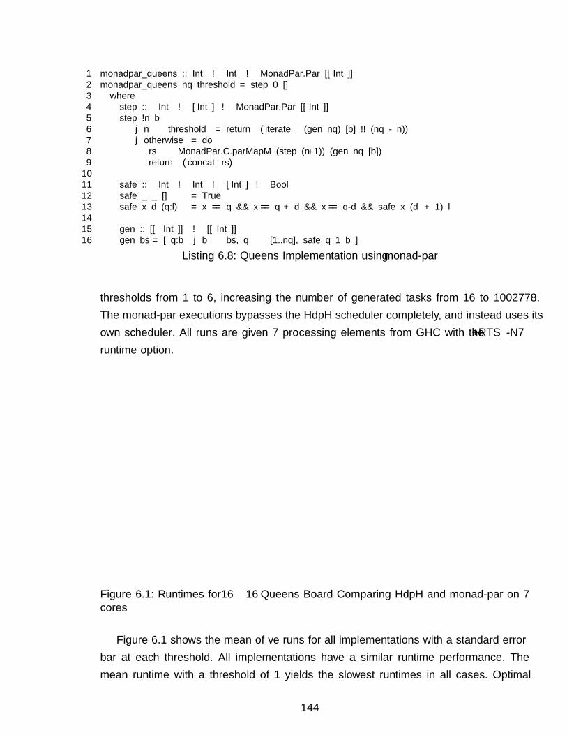
1 monadpar_queens :: Int → Int → MonadPar.Par [[Int]]2 monadpar_queens nq threshold = step 0 []3 where4 step :: Int → [Int] → MonadPar.Par [[Int]]5 step !n b6 | n ≥ threshold = return (iterate (gen nq) [b] !! (nq - n))7 | otherwise = do8 rs ← MonadPar.C.parMapM (step (n+1)) (gen nq [b])9 return (concat rs)1011 safe :: Int → Int → [Int] → Bool12 safe _ _ [] = True13 safe x d (q:l) = x /= q && x /= q + d && x /= q-d && safe x (d + 1) l1415 gen :: [[Int]] → [[Int]]16 gen bs = [ q:b | b ← bs, q ← [1..nq], safe q 1 b ]

Listing 6.8: Queens Implementation using monad-par

thresholds from 1 to 6, increasing the number of generated tasks from 16 to 1002778.The monad-par executions bypasses the HdpH scheduler completely, and instead uses itsown scheduler. All runs are given 7 processing elements from GHC with the +RTS -N7

runtime option.

●

●

● ●

●

●

170

180

190

200

210

220

2 4 6Threshold

Run

time

(Sec

onds

)

Variant

● fork

monad−par

spawn

supervisedSpawn

Runtime for Queens 16x16 on Beowulf, inreasing threshold from 1 to 6

Figure 6.1: Runtimes for 16 × 16 Queens Board Comparing HdpH and monad-par on 7cores

Figure 6.1 shows the mean of five runs for all implementations with a standard errorbar at each threshold. All implementations have a similar runtime performance. Themean runtime with a threshold of 1 yields the slowest runtimes in all cases. Optimal

144

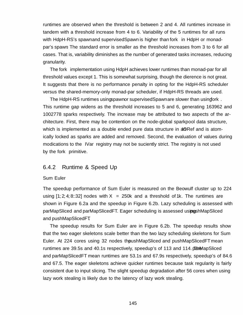
runtimes are observed when the threshold is between 2 and 4. All runtimes increase intandem with a threshold increase from 4 to 6. Variability of the 5 runtimes for all runswith HdpH-RS’s spawn and supervisedSpawn is higher than fork in HdpH or monad-par’s spawn. The standard error is smaller as the threshold increases from 3 to 6 for allcases. That is, variability diminishes as the number of generated tasks increases, reducinggranularity.

The fork implementation using HdpH achieves lower runtimes than monad-par for allthreshold values except 1. This is somewhat surprising, though the difference is not great.It suggests that there is no performance penalty in opting for the HdpH-RS schedulerversus the shared-memory-only monad-par scheduler, if HdpH-RS threads are used.

The HdpH-RS runtimes using spawn or supervisedSpawn are slower than using fork.This runtime gap widens as the threshold increases to 5 and 6, generating 163962 and1002778 sparks respectively. The increase may be attributed to two aspects of the ar-chitecture. First, there may be contention on the node-global sparkpool data structure,which is implemented as a double ended pure data structure in an IORef and is atom-ically locked as sparks are added and removed. Second, the evaluation of values duringmodifications to the IVar registry may not be sufficiently strict. The registry is not usedby the fork primitive.

6.4.2 Runtime & Speed Up

Sum Euler

The speedup performance of Sum Euler is measured on the Beowulf cluster up to 224using [1, 2, 4, 8..32] nodes with X = 250k and a threshold of 1k. The runtimes areshown in Figure 6.2a and the speedup in Figure 6.2b. Lazy scheduling is assessed withparMapSliced and parMapSlicedFT. Eager scheduling is assessed using pushMapSliced

and pushMapSlicedFT.The speedup results for Sum Euler are in Figure 6.2b. The speedup results show

that the two eager skeletons scale better than the two lazy scheduling skeletons for SumEuler. At 224 cores using 32 nodes the pushMapSliced and pushMapSlicedFT meanruntimes are 39.5s and 40.1s respectively, speedup’s of 113 and 114. The parMapSliced

and parMapSlicedFT mean runtimes are 53.1s and 67.9s respectively, speedup’s of 84.6and 67.5. The eager skeletons achieve quicker runtimes because task regularity is fairlyconsistent due to input slicing. The slight speedup degradation after 56 cores when usinglazy work stealing is likely due to the latency of lazy work stealing.

145

●

●

●

●

●●

● ● ● ● ●

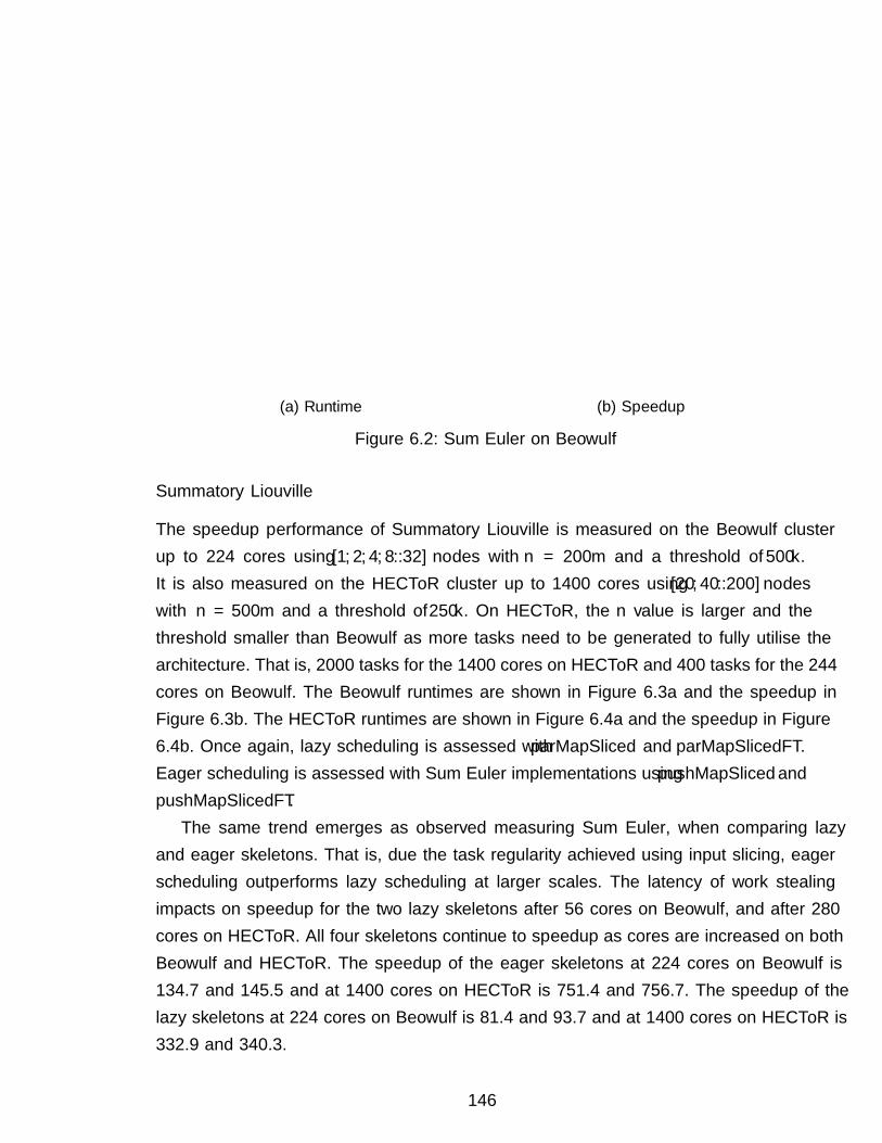
1000

2000

3000

4000

50 100 150 200Cores

Run

time

(Sec

onds

)

Variant

● parMapSliced

parMapSlicedFT

pushMapSliced

pushMapSlicedFT

Runtime for Sum Euler 0 to 250k on Beowulf, threshold=1k

(a) Runtime

●

●

●

●

●

●

●

●

●

● ●

30

60

90

50 100 150 200Cores

Spe

ed U

p

Variant

● parMapSliced

parMapSlicedFT

pushMapSliced

pushMapSlicedFT

Speedup for Sum Euler 0 to 250k on Beowulf, threshold=1k

(b) Speedup

Figure 6.2: Sum Euler on Beowulf

Summatory Liouville

The speedup performance of Summatory Liouville is measured on the Beowulf clusterup to 224 cores using [1, 2, 4, 8..32] nodes with n = 200m and a threshold of 500k.It is also measured on the HECToR cluster up to 1400 cores using [20, 40..200] nodeswith n = 500m and a threshold of 250k. On HECToR, the n value is larger and thethreshold smaller than Beowulf as more tasks need to be generated to fully utilise thearchitecture. That is, 2000 tasks for the 1400 cores on HECToR and 400 tasks for the 244cores on Beowulf. The Beowulf runtimes are shown in Figure 6.3a and the speedup inFigure 6.3b. The HECToR runtimes are shown in Figure 6.4a and the speedup in Figure6.4b. Once again, lazy scheduling is assessed with parMapSliced and parMapSlicedFT.Eager scheduling is assessed with Sum Euler implementations using pushMapSliced andpushMapSlicedFT.

The same trend emerges as observed measuring Sum Euler, when comparing lazyand eager skeletons. That is, due the task regularity achieved using input slicing, eagerscheduling outperforms lazy scheduling at larger scales. The latency of work stealingimpacts on speedup for the two lazy skeletons after 56 cores on Beowulf, and after 280cores on HECToR. All four skeletons continue to speedup as cores are increased on bothBeowulf and HECToR. The speedup of the eager skeletons at 224 cores on Beowulf is134.7 and 145.5 and at 1400 cores on HECToR is 751.4 and 756.7. The speedup of thelazy skeletons at 224 cores on Beowulf is 81.4 and 93.7 and at 1400 cores on HECToR is332.9 and 340.3.

146

●

●

●

●

● ● ● ● ● ● ●

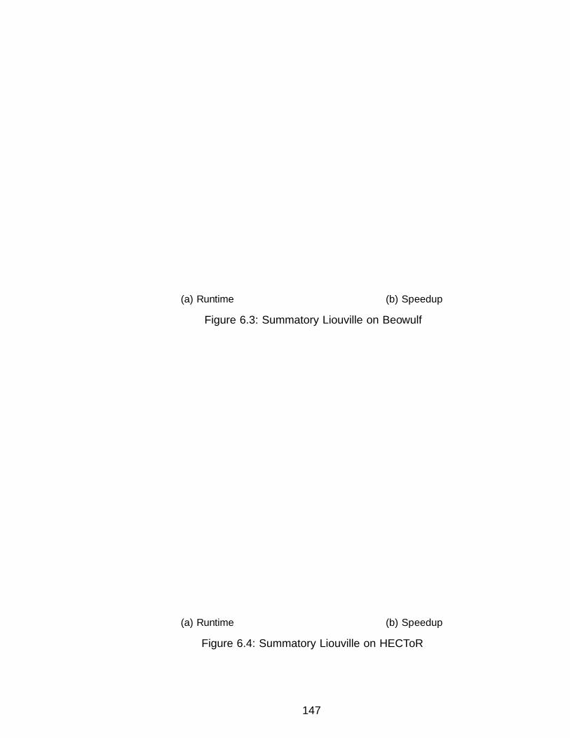
1000

2000

3000

50 100 150 200Cores

Run

time

(Sec

onds

)Variant

● parMapSliced

parMapSlicedFT

pushMapSliced

pushMapSlicedFT

Runtime for Summatory Liouville of 200m on Beowulf, threshold=500k

(a) Runtime

●

●

●

●

●

●

●

●

●

●

●

50

100

50 100 150 200Cores

Spe

ed U

p

Variant

● parMapSliced

parMapSlicedFT

pushMapSliced

pushMapSlicedFT

Speedup for Summatory Liouville of 200m on Beowulf, threshold=500k

(b) Speedup

Figure 6.3: Summatory Liouville on Beowulf

●

● ● ● ● ● ● ● ● ● ●

2500

5000

7500

10000

12500

500 1000Cores

Run

time

(Sec

onds

)

Variant

● parMapSliced

parMapSlicedFT

pushMapSliced

pushMapSlicedFT

Runtime for Summatory Liouville of 500m on HECToR, threshold=250k

(a) Runtime

●

●

●

●

●

●

●

●● ●

●

200

400

600

500 1000Cores

Spe

ed U

p

Variant

● parMapSliced

parMapSlicedFT

pushMapSliced

pushMapSlicedFT

Speedup for Summatory Liouville of 500m on HECToR, threshold=250k

(b) Speedup

Figure 6.4: Summatory Liouville on HECToR

147

●

●

●

●

● ● ● ● ● ● ●

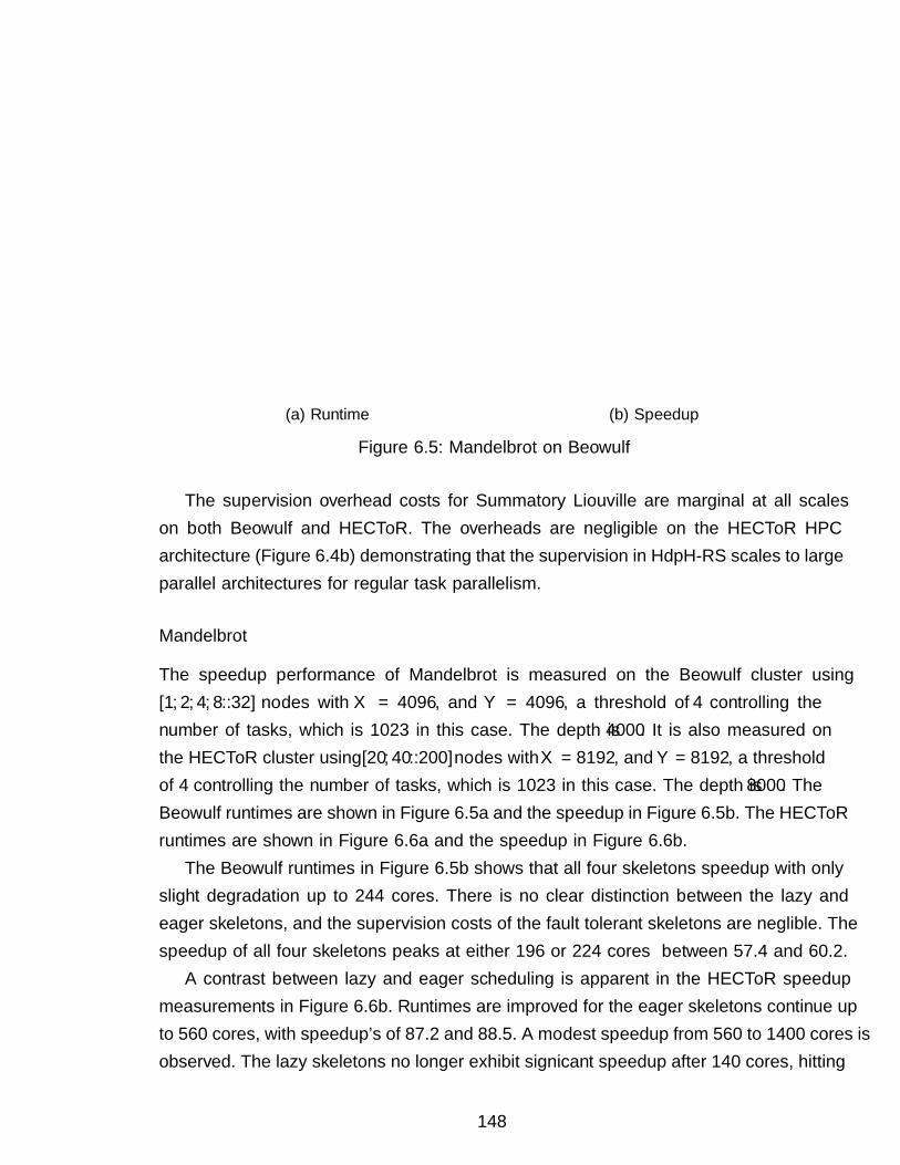
500

1000

1500

2000

2500

50 100 150 200Cores

Run

time

(Sec

onds

)

Variant

● parMapReduceRangeThresh

parMapReduceRangeThreshFT

pushMapReduceRangeThresh

pushMapReduceRangeThreshFT

Runtime for Mandebrot 4096x4096 on Beowulf, threshold=4, depth=4000

(a) Runtime

●

●

●

●

●

●

●

●

●

●●

10

20

30

40

50

60

50 100 150 200Cores

Spe

ed U

p

Variant

● parMapReduceRangeThresh

parMapReduceRangeThreshFT

pushMapReduceRangeThresh

pushMapReduceRangeThreshFT

Speedup for Mandebrot 4096x4096 on Beowulf, threshold=4, depth=4000

(b) Speedup

Figure 6.5: Mandelbrot on Beowulf

The supervision overhead costs for Summatory Liouville are marginal at all scaleson both Beowulf and HECToR. The overheads are negligible on the HECToR HPCarchitecture (Figure 6.4b) demonstrating that the supervision in HdpH-RS scales to largeparallel architectures for regular task parallelism.

Mandelbrot

The speedup performance of Mandelbrot is measured on the Beowulf cluster using[1, 2, 4, 8..32] nodes with X = 4096, and Y = 4096, a threshold of 4 controlling thenumber of tasks, which is 1023 in this case. The depth is 4000. It is also measured onthe HECToR cluster using [20, 40..200] nodes with X = 8192, and Y = 8192, a thresholdof 4 controlling the number of tasks, which is 1023 in this case. The depth is 8000. TheBeowulf runtimes are shown in Figure 6.5a and the speedup in Figure 6.5b. The HECToRruntimes are shown in Figure 6.6a and the speedup in Figure 6.6b.

The Beowulf runtimes in Figure 6.5b shows that all four skeletons speedup with onlyslight degradation up to 244 cores. There is no clear distinction between the lazy andeager skeletons, and the supervision costs of the fault tolerant skeletons are neglible. Thespeedup of all four skeletons peaks at either 196 or 224 cores — between 57.4 and 60.2.

A contrast between lazy and eager scheduling is apparent in the HECToR speedupmeasurements in Figure 6.6b. Runtimes are improved for the eager skeletons continue upto 560 cores, with speedup’s of 87.2 and 88.5. A modest speedup from 560 to 1400 cores isobserved. The lazy skeletons no longer exhibit significant speedup after 140 cores, hitting

148

●

● ● ● ● ● ● ● ● ● ●

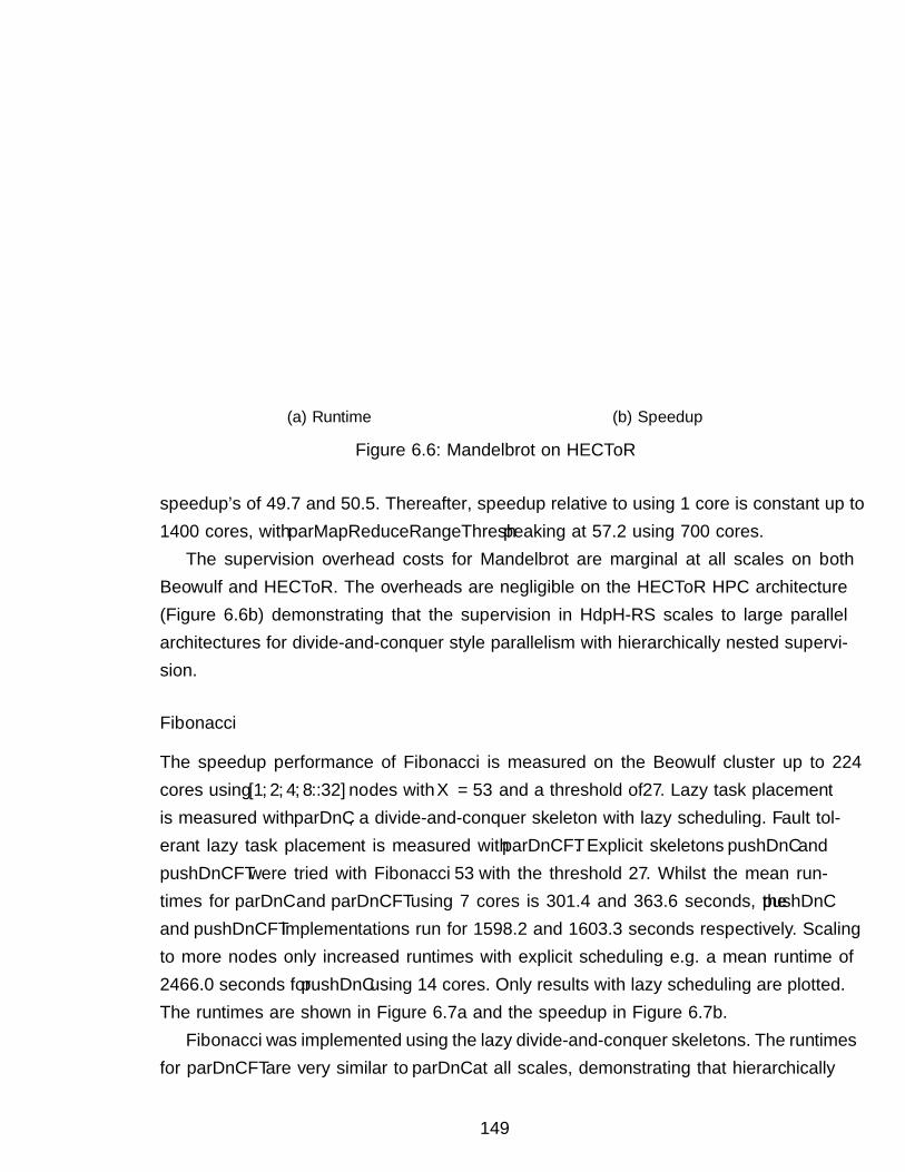
2000

4000

6000

500 1000Cores

Run

time

(Sec

onds

)

Variant

● parMapReduceRangeThresh

parMapReduceRangeThreshFT

pushMapReduceRangeThresh

pushMapReduceRangeThreshFT

Runtime for Mandebrot 4096x4096 on HECToR, threshold=4, depth=8000

(a) Runtime

●

●●

●

●

●

●●

●

●●

25

50

75

500 1000Cores

Spe

ed U

p

Variant

● parMapReduceRangeThresh

parMapReduceRangeThreshFT

pushMapReduceRangeThresh

pushMapReduceRangeThreshFT

Speedup for Mandebrot 4096x4096 on HECToR, threshold=4, depth=8000

(b) Speedup

Figure 6.6: Mandelbrot on HECToR

speedup’s of 49.7 and 50.5. Thereafter, speedup relative to using 1 core is constant up to1400 cores, with parMapReduceRangeThresh peaking at 57.2 using 700 cores.

The supervision overhead costs for Mandelbrot are marginal at all scales on bothBeowulf and HECToR. The overheads are negligible on the HECToR HPC architecture(Figure 6.6b) demonstrating that the supervision in HdpH-RS scales to large parallelarchitectures for divide-and-conquer style parallelism with hierarchically nested supervi-sion.

Fibonacci

The speedup performance of Fibonacci is measured on the Beowulf cluster up to 224cores using [1, 2, 4, 8..32] nodes with X = 53 and a threshold of 27. Lazy task placementis measured with parDnC, a divide-and-conquer skeleton with lazy scheduling. Fault tol-erant lazy task placement is measured with parDnCFT. Explicit skeletons pushDnC andpushDnCFT were tried with Fibonacci 53 with the threshold 27. Whilst the mean run-times for parDnC and parDnCFT using 7 cores is 301.4 and 363.6 seconds, the pushDnC

and pushDnCFT implementations run for 1598.2 and 1603.3 seconds respectively. Scalingto more nodes only increased runtimes with explicit scheduling e.g. a mean runtime of2466.0 seconds for pushDnC using 14 cores. Only results with lazy scheduling are plotted.The runtimes are shown in Figure 6.7a and the speedup in Figure 6.7b.

Fibonacci was implemented using the lazy divide-and-conquer skeletons. The runtimesfor parDnCFT are very similar to parDnC at all scales, demonstrating that hierarchically

149

●

●

●

● ●

● ● ● ● ● ●

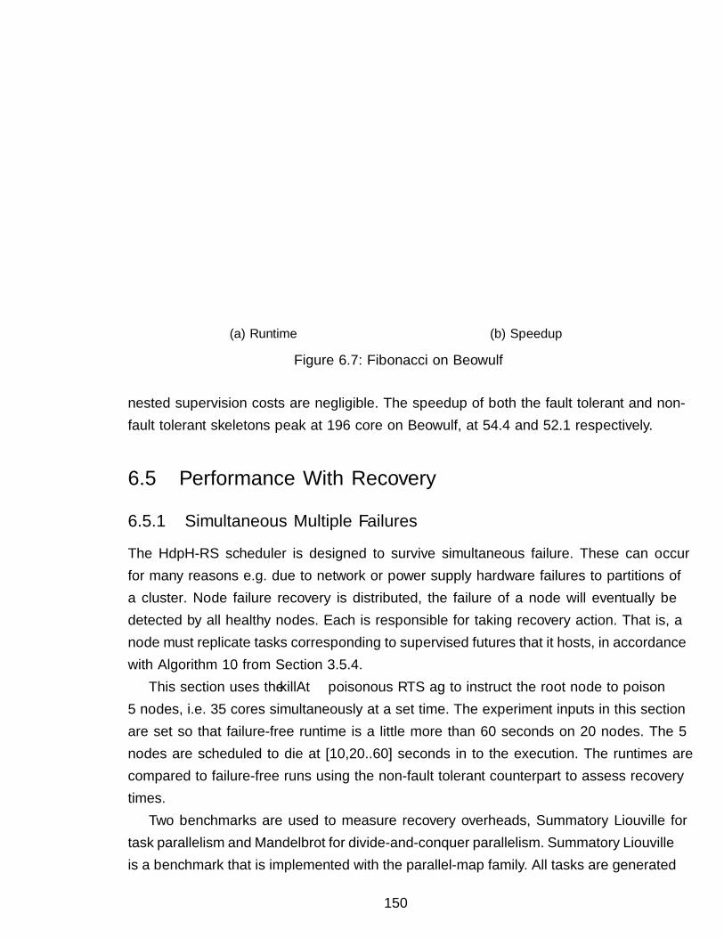
500

1000

1500

2000

50 100 150 200Cores

Run

time

(Sec

onds

)

Variant

● parDnC

parDnCFT

Runtime for Fibonacci 53 on Beowulf, threshold=27

(a) Runtime

●

●

●

● ●

●

●

●

●

●

●

10

20

30

40

50

50 100 150 200Cores

Spe

ed U

p

Variant

● parDnC

parDnCFT

Speedup for Fibonacci 53 on Beowulf, threshold=27

(b) Speedup

Figure 6.7: Fibonacci on Beowulf

nested supervision costs are negligible. The speedup of both the fault tolerant and non-fault tolerant skeletons peak at 196 core on Beowulf, at 54.4 and 52.1 respectively.

6.5 Performance With Recovery

6.5.1 Simultaneous Multiple Failures

The HdpH-RS scheduler is designed to survive simultaneous failure. These can occurfor many reasons e.g. due to network or power supply hardware failures to partitions ofa cluster. Node failure recovery is distributed, the failure of a node will eventually bedetected by all healthy nodes. Each is responsible for taking recovery action. That is, anode must replicate tasks corresponding to supervised futures that it hosts, in accordancewith Algorithm 10 from Section 3.5.4.

This section uses the killAt poisonous RTS flag to instruct the root node to poison5 nodes, i.e. 35 cores simultaneously at a set time. The experiment inputs in this sectionare set so that failure-free runtime is a little more than 60 seconds on 20 nodes. The 5nodes are scheduled to die at [10,20..60] seconds in to the execution. The runtimes arecompared to failure-free runs using the non-fault tolerant counterpart to assess recoverytimes.

Two benchmarks are used to measure recovery overheads, Summatory Liouville fortask parallelism and Mandelbrot for divide-and-conquer parallelism. Summatory Liouvilleis a benchmark that is implemented with the parallel-map family. All tasks are generated

150

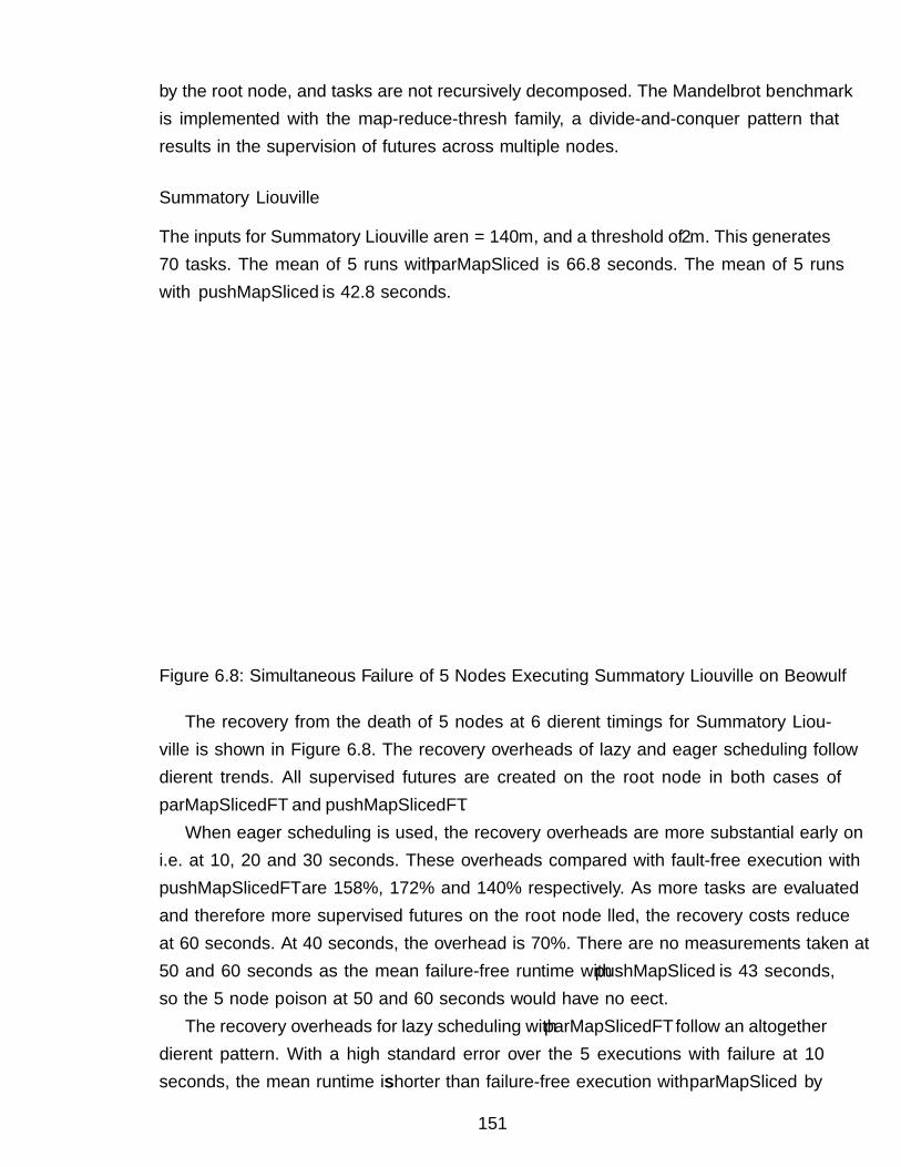
by the root node, and tasks are not recursively decomposed. The Mandelbrot benchmarkis implemented with the map-reduce-thresh family, a divide-and-conquer pattern thatresults in the supervision of futures across multiple nodes.

Summatory Liouville

The inputs for Summatory Liouville are n = 140m, and a threshold of 2m. This generates70 tasks. The mean of 5 runs with parMapSliced is 66.8 seconds. The mean of 5 runswith pushMapSliced is 42.8 seconds.

●

●

●

●

●

●

parMapSliced

pushMapSliced

40

60

80

100

120

20 40 60Time of Simultanous 5 Node Failure (Seconds)

Run

time

(Sec

onds

)

Variant

● parMapSlicedFT

pushMapSlicedFT

Runtime for Summatory Liouville of 140m on Beowulf, threshold=2m

Figure 6.8: Simultaneous Failure of 5 Nodes Executing Summatory Liouville on Beowulf

The recovery from the death of 5 nodes at 6 different timings for Summatory Liou-ville is shown in Figure 6.8. The recovery overheads of lazy and eager scheduling followdifferent trends. All supervised futures are created on the root node in both cases ofparMapSlicedFT and pushMapSlicedFT.

When eager scheduling is used, the recovery overheads are more substantial early oni.e. at 10, 20 and 30 seconds. These overheads compared with fault-free execution withpushMapSlicedFT are 158%, 172% and 140% respectively. As more tasks are evaluatedand therefore more supervised futures on the root node filled, the recovery costs reduceat 60 seconds. At 40 seconds, the overhead is 70%. There are no measurements taken at50 and 60 seconds as the mean failure-free runtime with pushMapSliced is 43 seconds,so the 5 node poison at 50 and 60 seconds would have no effect.

The recovery overheads for lazy scheduling with parMapSlicedFT follow an altogetherdifferent pattern. With a high standard error over the 5 executions with failure at 10seconds, the mean runtime is shorter than failure-free execution with parMapSliced by

151

14%. Unlike eager task placement, this is likely due to a much smaller number of the70 generated sparks being fished by the 5 nodes that had failed after only 10 seconds.Moreover, it is likely that the balance between computation and communication for thejob size with n = 140m favours smaller cluster than 20 nodes, i.e. the 15 nodes that areleft. As the delay until failure is increased to 20, 30, 40 and 50 seconds, the recoveryoverheads are 2%, 13%, 18% and 22%. As most supervised futures on the root nodebecome full at the 60 second failure executions, fewer sparks need replicating. Thus, theruntimes with failure at 60 seconds are close to the failure-free runtimes, resulting in asmall speedup of 3%.

Mandelbrot

The inputs for Mandelbrot are X = 4096, Y = 4096, threshold = 4 and depth = 4000.This generates 1023 tasks. The mean of 5 runs with parMapReduceRangeThresh is 66seconds. The mean of 5 runs with pushMapReduceRangeThresh is 92 seconds.

●

●

●

●

●

●

parMapReduceRangeThresh

pushMapReduceRangeThresh

50

100

150

200

20 40 60Time of Simultanous 5 Node Failure (Seconds)

Run

time

(Sec

onds

)

Variant

● parMapReduceRangeThreshFT

pushMapReduceRangeThreshFT

Runtime for Mandel 4096x4096 on Beowulf, Depth=4000

Figure 6.9: Simultaneous Failure of 5 Nodes Executing Mandelbrot on Beowulf

The recovery from the death of 5 nodes at the 6 different timings for Mandelbrotis shown in Figure 6.9, and reveals two distinct trends. The recovery overheads for thelazy parMapReduceRangeThreshFT skeleton are low, even as the number of generatedsupervised futures increases. The mean runtime when 5 nodes are killed at 60 seconds ismarginally shorter by 3.0 seconds than failure-free execution with 20 nodes, a speedupof 5%.

The recovery overheads for the eager pushMapReduceRangeThreshFT skeleton in-creases as more threads are replicated needlessly (Section 6.5.3). Early failures of 10

152

seconds shortens runtime by 10%. The eventual total of 1023 threads will likely not havebeen created by this point, and balance between communication and computation forthe inputs of X = 4096 and Y = 4096 may favour the smaller 15 node cluster size. How-ever, when the 5 node failure occurs at 20, 30, 40, 50 and 60 seconds, the recovery costsincrease. For these times, the recovery overheads are 44%, 18%, 59%, 80% and 110%.

6.5.2 Chaos Monkey

A unit testing suite is built-in to eight benchmarks (Table 6.5) to check that resultscomputed by HdpH-RS in the presence of random failure are correct. Sum Euler isused to measure recovery costs of parMapChunkedFT and pushMapChunkedFT, Sum-matory Liouville to asses parMapSlicedFT and pushMapSlicedFT, Queens to measureparDnCFT and pushDnCFT and Mandelbrot to assess parMapReduceRangeThreshFT andpushMapReduceRangeThreshFT. The unit tests are invoked when the chaosMonkey flag isused. The chaos monkey failure injection exploits the UDP peer discovery in HdpH-RS,and is shown in Listing 6.9. The chaosMonkeyPoison function on line 8 is executed bythe root node. It randomly decides how many of the non-root nodes will be poisoned(line 10), and the timing of failure in each case (line 11). These messages are sent to arandomly sorted node sequence.

The executing code on non-root nodes is run on line 19. A non-root node waits for aBooted message on line 21. If a Booted Nothing message is received then it is ignored.If a Booted (Just x) message is received, then a suicidal thread is forked on line 24. Itwill kill the node at x seconds in to the job execution.

The HUnit test framework [80] is used in the HdpH-RS function chaosMonkeyUnitTestshown in Listing 6.10 and verifies that the fault tolerant skeletons return the correct resultwith chaos monkey enabled. For example, the chaosMonkeyUnitTest takes a HdpH-RSRTS configuration, a String label for the test e.g. "sumeuler-0-50k-chaos-monkey", thenan expected value 759924264 for a parallel Sum Euler 0 to 50000 computation in the Parmonad. The implementation of chaosMonkeyUnitTest is in Appendix A.10.

An execution of Sum Euler with the fault tolerant pushMapChunkedFT skeleton isshown in Listing 6.11. It asks for 5 node instances from mpiexec with the -N 5 flag,and HdpH-RS is told discover 5 nodes via UDP with -numProcs=5. MPI is forced toignore a node failure with the --disable-auto-cleanup flag. The chaosMonkey flagturns on random node failure. The root node non-deterministically decides that 3 nodesshall fail. The first will fail at 4 seconds, the second at 23 seconds and the third at 36seconds. When failure is detected, the at-risk threads on the failed node are re-scheduled.There are no sparks to re-schedule because pushMapChunkedFT is entirely explicit, using

153

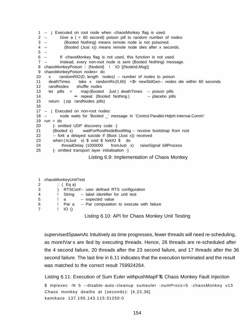
1 -- | Executed on root node when -chaosMonkey flag is used.2 -- Give a (< 60 second) poison pill to random number of nodes:3 -- (Booted Nothing) means remote node is not poisoned.4 -- (Booted (Just x)) means remote node dies after x seconds.5 --6 -- If -chaosMonkey flag is not used, this function is not used.7 -- Instead, every non-root node is sent (Booted Nothing) message.8 chaosMonkeyPoison :: [NodeId] → IO [(NodeId,Msg)]9 chaosMonkeyPoison nodes = do10 x ← randomRIO (0,length nodes) -- number of nodes to poison11 deathTimes ← take x ◦ randomRs (0,60) <$> newStdGen -- nodes die within 60 seconds12 randNodes ← shuffle nodes13 let pills = map (Booted ◦ Just) deathTimes -- poison pills14 ++ repeat (Booted Nothing) -- placebo pills15 return (zip randNodes pills)1617 -- | Executed on non-root nodes:18 -- node waits for ’Booted _’ message in ’Control.Parallel.HdpH.Internal.Comm’19 run = do20 {- omitted UDP discovery code -}21 (Booted x) ← waitForRootNodeBootMsg -- receive bootstrap from root22 -- fork a delayed suicide if (Boot (Just x)) received23 when (isJust x) $ void $ forkIO $ do24 threadDelay (1000000 ∗ fromJust x) » raiseSignal killProcess25 {- omitted transport layer initialisation -}

Listing 6.9: Implementation of Chaos Monkey

1 chaosMonkeyUnitTest2 :: (Eq a)3 ⇒ RTSConf -- user defined RTS configuration4 → String -- label identifier for unit test5 → a -- expected value6 → Par a -- Par computation to execute with failure7 → IO ()

Listing 6.10: API for Chaos Monkey Unit Testing

supervisedSpawnAt. Intuitively as time progresses, fewer threads will need re-scheduling,as more IVars are filled by executing threads. Hence, 26 threads are re-scheduled afterthe 4 second failure, 20 threads after the 23 second failure, and 17 threads after the 36second failure. The last line in 6.11 indicates that the execution terminated and the resultwas matched to the correct result 759924264.

Listing 6.11: Execution of Sum Euler with pushMapFT & Chaos Monkey Fault Injection$ mpiexec -N 5 --disable -auto -cleanup sumeuler -numProcs =5 -chaosMonkey v13

Chaos monkey deaths at (seconds ): [4 ,23 ,36]

kamikaze 137.195.143.115:31250:0

154

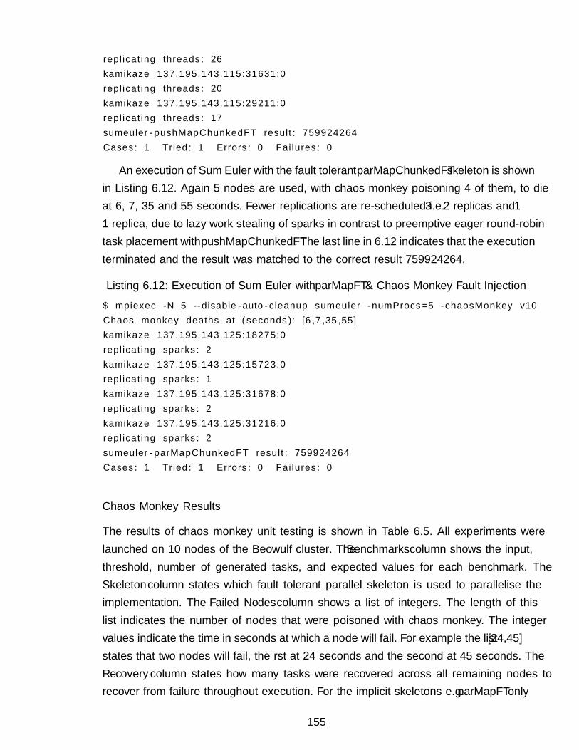
replicating threads: 26

kamikaze 137.195.143.115:31631:0

replicating threads: 20

kamikaze 137.195.143.115:29211:0

replicating threads: 17

sumeuler -pushMapChunkedFT result: 759924264

Cases: 1 Tried: 1 Errors: 0 Failures: 0

An execution of Sum Euler with the fault tolerant parMapChunkedFT skeleton is shownin Listing 6.12. Again 5 nodes are used, with chaos monkey poisoning 4 of them, to dieat 6, 7, 35 and 55 seconds. Fewer replications are re-scheduled i.e. 3× 2 replicas and 1×1 replica, due to lazy work stealing of sparks in contrast to preemptive eager round-robintask placement with pushMapChunkedFT. The last line in 6.12 indicates that the executionterminated and the result was matched to the correct result 759924264.

Listing 6.12: Execution of Sum Euler with parMapFT & Chaos Monkey Fault Injection$ mpiexec -N 5 --disable -auto -cleanup sumeuler -numProcs =5 -chaosMonkey v10

Chaos monkey deaths at (seconds ): [6,7,35,55]

kamikaze 137.195.143.125:18275:0

replicating sparks: 2

kamikaze 137.195.143.125:15723:0

replicating sparks: 1

kamikaze 137.195.143.125:31678:0

replicating sparks: 2

kamikaze 137.195.143.125:31216:0

replicating sparks: 2

sumeuler -parMapChunkedFT result: 759924264

Cases: 1 Tried: 1 Errors: 0 Failures: 0

Chaos Monkey Results

The results of chaos monkey unit testing is shown in Table 6.5. All experiments werelaunched on 10 nodes of the Beowulf cluster. The Benchmarks column shows the input,threshold, number of generated tasks, and expected values for each benchmark. TheSkeleton column states which fault tolerant parallel skeleton is used to parallelise theimplementation. The Failed Nodes column shows a list of integers. The length of thislist indicates the number of nodes that were poisoned with chaos monkey. The integervalues indicate the time in seconds at which a node will fail. For example the list [24,45]states that two nodes will fail, the first at 24 seconds and the second at 45 seconds. TheRecovery column states how many tasks were recovered across all remaining nodes torecover from failure throughout execution. For the implicit skeletons e.g. parMapFT only

155

sparks are generated and thus recovered. For the implicit skeletons e.g. pushMapFT onlythreads are generated and recovered. The Runtime column shows the runtime for eachexecution. Lastly, the Unit Test column states whether the result from HdpH-RS in thepresence of failure matched the pre-computed result using HdpH with no failure. Thetest-suite passes 100% of the unit tests.

The key observation from these results is that lazy scheduling reduces recoverycosts in the presence of failure. The parDnCFT skeleton (divide-and-conquer usingsupervisedSpawn) creates only sparks, initially on the root node, which get fished awaywith work stealing. The pushDnCFT skeleton uses supervisedSpawnAt to randomly selectnodes to eagerly scheduled tasks as threads. The laziness of supervisedSpawn minimisesthe migration of sparks, taking place only when nodes become idle. It also minimises thenumber of sparks that need to be recovered. For example, the Queens unit test generates65234 tasks. The pushDnCFT results in the re-scheduling of 40696 threads in the case ofbetween 1 and 3 node failures at [3, 15, 15] before the execution would have likely ter-minated at 15 seconds. Subsequent node failures at [23, 24, 28, 32, 48] seconds may haveresulted in multiple replicas of tasks being eagerly scheduled as earlier scheduled replicasmay have also been lost. The runtime to termination is 650 seconds. The Queens unittest with parDnCFT results in the re-scheduling of only 8 sparks in another case of 5 likelynode failures at [3, 8, 9, 10, 17] before the execution would have likely terminated at 28seconds. Subsequent node failures at [45, 49, 51] seconds may have resulted in multiplereplicas of tasks being lazily scheduled as earlier scheduled replicas may have also beenlost. The runtime to termination is 52 seconds. An explanation for the much lower impactof failure when on-demand work stealing is used is given in Section 6.5.3.

On-demand work stealing also manages the trade off between communication andcomputation by reducing unnecessary task scheduling to remote nodes if task granularityis very small. The Mandelbrot benchmark is used to demonstrate this. The depth is setat 256, a relatively low number that generates small task sizes (the speed-up is latermeasured in Section 6.4.2 using a depth of 4000). The small Mandelbrot task sizes in thechaos monkey experiments mean that very few sparks are replicated as most are executedby the root node. In 3 runs, 0 sparks are replicated including an execution with 8 nodefailures. In contrast, 686 threads are replicated with a failure accumulation of 8 nodes,when eager scheduling pushes tasks to remote nodes regardless of task size.

6.5.3 Increasing Recovery Overheads with Eager Scheduling

The lazy task scheduling with parMapChunkedFT for Sum Euler, parMapSlicedFT forSummatory Liouville, parDnCFT for Queens, and parMapReduceFT for Mandelbrot result

156

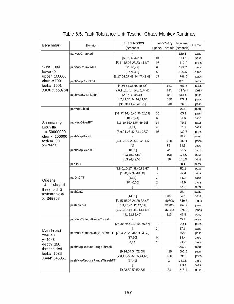
Table 6.5: Fault Tolerance Unit Testing: Chaos Monkey Runtimes

Benchmark SkeletonFailed Nodes Recovery Runtime Unit Test

(seconds) Sparks Threads (seconds)

parMapChunked - 126.1 pass

Sum Eulerlower=0upper=100000chunk=100tasks=1001X=3039650754

parMapChunkedFT

[6,30,39,49,50] 10 181.1 pass[5,11,18,27,28,33,44,60] 16 410.2 pass

[31,36,49] 6 139.7 pass[37,48,59] 6 139.5 pass

[1,17,24,27,43,44,47,48,48] 17 768.2 passpushMapChunked - 131.6 pass

pushMapChunkedFT

[4,34,36,37,48,49,58] 661 753.7 pass[2,6,11,15,17,24,32,37,41] 915 1179.7 pass

[2,37,39,45,49] 481 564.0 pass[4,7,23,32,34,46,54,60] 760 978.1 pass

[35,38,41,43,46,51] 548 634.3 passparMapSliced - 56.6 pass

SummatoryLiouvilleλ = 50000000chunk=100000tasks=500X=-7608

parMapSlicedFT

[32,37,44,46,48,50,52,57] 16 85.1 pass[18,27,41] 6 61.6 pass

[19,30,39,41,54,59,59] 14 76.2 pass[8,11] 4 62.8 pass

[8,9,24,28,32,34,40,57] 16 132.7 passpushMapSliced - 58.3 pass

pushMapSlicedFT

[3,8,8,12,22,26,26,29,55] 268 287.1 pass[1] 53 63.3 pass

[10,59] 41 68.5 pass[13,15,18,51] 106 125.0 pass[13,24,42,51] 80 105.9 pass

parDnC - 28.1 pass

Queens14× 14 boardthreshold=5tasks=65234X=365596

parDnCFT

[3,8,9,10,17,45,49,51,57] 8 52.1 pass[1,30,32,33,48,50] 5 49.4 pass

[8,15] 2 53.3 pass[20,40,56] 2 49.9 pass

[] 0 52.8 passpushDnC - 15.4 pass

pushDnCFT

[14,33] 5095 57.1 pass[3,15,15,23,24,28,32,48] 40696 649.5 pass

[5,8,26,41,42,42,59] 36305 354.9 pass[0,5,8,10,14,28,31,51,54] 32629 276.9 pass

[31,31,58,60] 113 47.8 passparMapReduceRangeThresh - 23.2 pass

Mandelbrotx=4048y=4048depth=256threshold=4tasks=1023X=449545051

parMapReduceRangeThreshFT

[28,30,36,44,49,54,56,56] 0 29.1 pass[] 0 27.8 pass

[7,24,25,25,44,53,54,59] 6 32.6 pass[17,30] 0 55.4 pass[0,14] 2 33.7 pass

pushMapReduceRangeThresh - 366.3 pass

pushMapReduceRangeThreshFT

[9,24,34,34,52,59] 419 205.3 pass[7,8,11,22,32,35,44,46] 686 395.9 pass

[27,49] 2 371.8 pass[] 0 380.4 pass

[9,33,50,50,52,53] 84 216.1 pass

157

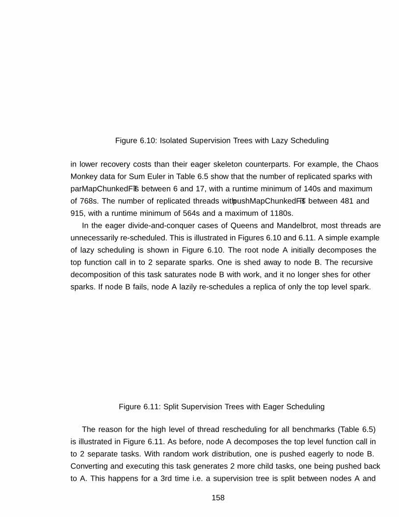
SCHEDULE

Node A Node B

Supervised SparkReplicated Once

1

Figure 6.10: Isolated Supervision Trees with Lazy Scheduling

in lower recovery costs than their eager skeleton counterparts. For example, the ChaosMonkey data for Sum Euler in Table 6.5 show that the number of replicated sparks withparMapChunkedFT is between 6 and 17, with a runtime minimum of 140s and maximumof 768s. The number of replicated threads with pushMapChunkedFT is between 481 and915, with a runtime minimum of 564s and a maximum of 1180s.

In the eager divide-and-conquer cases of Queens and Mandelbrot, most threads areunnecessarily re-scheduled. This is illustrated in Figures 6.10 and 6.11. A simple exampleof lazy scheduling is shown in Figure 6.10. The root node A initially decomposes thetop function call in to 2 separate sparks. One is fished away to node B. The recursivedecomposition of this task saturates node B with work, and it no longer fishes for othersparks. If node B fails, node A lazily re-schedules a replica of only the top level spark.

PUSH

Node A Node B

Thread ReplicatedMore Than Once

Thread ReplicatedOnce

3

2

2

1

1

Figure 6.11: Split Supervision Trees with Eager Scheduling

The reason for the high level of thread rescheduling for all benchmarks (Table 6.5)is illustrated in Figure 6.11. As before, node A decomposes the top level function call into 2 separate tasks. With random work distribution, one is pushed eagerly to node B.Converting and executing this task generates 2 more child tasks, one being pushed backto A. This happens for a 3rd time i.e. a supervision tree is split between nodes A and

158

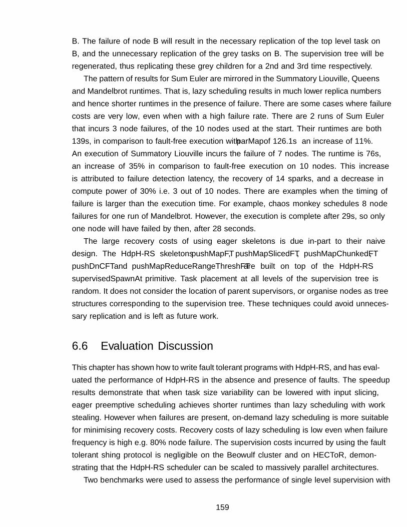
B. The failure of node B will result in the necessary replication of the top level task onB, and the unnecessary replication of the grey tasks on B. The supervision tree will beregenerated, thus replicating these grey children for a 2nd and 3rd time respectively.

The pattern of results for Sum Euler are mirrored in the Summatory Liouville, Queensand Mandelbrot runtimes. That is, lazy scheduling results in much lower replica numbersand hence shorter runtimes in the presence of failure. There are some cases where failurecosts are very low, even when with a high failure rate. There are 2 runs of Sum Eulerthat incurs 3 node failures, of the 10 nodes used at the start. Their runtimes are both139s, in comparison to fault-free execution with parMap of 126.1s — an increase of 11%.An execution of Summatory Liouville incurs the failure of 7 nodes. The runtime is 76s,an increase of 35% in comparison to fault-free execution on 10 nodes. This increaseis attributed to failure detection latency, the recovery of 14 sparks, and a decrease incompute power of 30% i.e. 3 out of 10 nodes. There are examples when the timing offailure is larger than the execution time. For example, chaos monkey schedules 8 nodefailures for one run of Mandelbrot. However, the execution is complete after 29s, so onlyone node will have failed by then, after 28 seconds.

The large recovery costs of using eager skeletons is due in-part to their naivedesign. The HdpH-RS skeletons pushMapFT, pushMapSlicedFT, pushMapChunkedFT,pushDnCFT and pushMapReduceRangeThreshFT are built on top of the HdpH-RSsupervisedSpawnAt primitive. Task placement at all levels of the supervision tree israndom. It does not consider the location of parent supervisors, or organise nodes as treestructures corresponding to the supervision tree. These techniques could avoid unneces-sary replication and is left as future work.

6.6 Evaluation Discussion

This chapter has shown how to write fault tolerant programs with HdpH-RS, and has eval-uated the performance of HdpH-RS in the absence and presence of faults. The speedupresults demonstrate that when task size variability can be lowered with input slicing,eager preemptive scheduling achieves shorter runtimes than lazy scheduling with workstealing. However when failures are present, on-demand lazy scheduling is more suitablefor minimising recovery costs. Recovery costs of lazy scheduling is low even when failurefrequency is high e.g. 80% node failure. The supervision costs incurred by using the faulttolerant fishing protocol is negligible on the Beowulf cluster and on HECToR, demon-strating that the HdpH-RS scheduler can be scaled to massively parallel architectures.

Two benchmarks were used to assess the performance of single level supervision with

159

parallel-map skeletons and three were used to assess hierarchically nested supervisionwith map-reduce and divide-and-conquer skeletons. These were executed on 244 cores ofa 32 node Beowulf cluster, and 1400 cores on HECToR.

The Sum Euler and Summatory Liouville benchmarks were implemented with lazyand eager parallel-map skeletons and input slicing was used to regulate task sizes. Thisflattening of task sizes diminished the need for lazy work stealing. As a result, the fault tol-erant eager scheduling achieved better speedup’s at scale. A speedup of 114 was achievedusing explicit scheduling of Sum Euler executed on Beowulf using 224 cores, and 68 withlazy scheduling. A speedup of 146 was achieved using explicit scheduling of SummatoryLiouville, and 94 with lazy scheduling. A speedup of 757 was achieved using explicitscheduling of Summatory Liouville on HECToR using 1400 cores, and 340 with lazyscheduling.

The Mandelbrot benchmark is implemented with lazy and eager map-reduce skeletons.There is no clear distinction between the lazy and eager skeletons executed on Beowulf.The speedup of all four skeletons peaks at either 196 or 224 cores — between 57.4 and60.2. A contrast between lazy and eager scheduling is apparent in the HECToR speedupmeasurements. Runtimes improve for the eager skeletons, continuing up to 560 coreswith a speedup of 88.5. A modest speedup from 560 to 1400 cores is observed thereafter.The lazy skeleton no longer exhibits significant speedup after 140 cores, peaking with aspeedup of 50.5.

Fibonacci was implemented using the lazy divide-and-conquer skeletons. The runtimesfor parDnCFT and very similar to parDnC at all scales. As with Mandelbrot, Fibonaccidemonstrates that hierarchically nested supervision costs are negligible. The speedup ofboth the fault tolerant and non-fault tolerant skeletons peak at 196 core on Beowulf, at54.4 and 52.1 respectively.

Four benchmarks are used to assess the resiliency of the parallel-map, map-reduceand divide-and-conquer skeletons in the presence of randomised Chaos Monkey failure.The executions with fault occurrence were executed on Beowulf — a platform that,unlike HECToR, supports the UDP peer discovery in the fault detecting TCP-basedHdpH-RS transport layer. The key observation from these results is that lazy schedulingreduces recovery costs in the presence of frequent failure. Lazy skeletons generate sparksthat are only scheduled elsewhere if requested through on-demand work stealing. Thislaziness minimises the migration of sparks, taking place only when nodes become idle.Eager skeletons preemptively distribute work from the task generating nodes, regardlessof work load of other nodes. Lazy scheduling therefore minimises the number of tasksthat need to be recovered when failures are detected.

160

For example, the Queens unit test generates 65234 tasks. Using the eager pushDnCFTskeleton results in the re-scheduling of 40696 threads in an execution during which 8 ofthe initial 10 nodes fail. This leads to an increased runtime of 649 seconds compared tothe mean 15 seconds of 5 failure-free pushDnC runtimes. In contrast, an execution usingthe lazy parDnCFT skeleton in the presence of 9 node failures results in the re-schedulingof only 8 sparks. This leads to a much lower recovery overhead with the runtime of 52seconds, compared to the mean 28 seconds of 5 failure-free parDnC runtimes.

161

Chapter 7

Conclusion

7.1 Summary

New approaches to language design and system architecture are needed to address thegrowing issue of fault tolerance for massively parallel heterogeneous architectures. Thisthesis investigates the challenges of providing reliable scalable symbolic computing. Ithas culminated in the design, validation and implementation of a Reliable Schedulingextension called HdpH-RS.

Chapter 2 presents a critical review of fault tolerance in distributed computing sys-tems, defining dependability terms (Section 2.1) and common existing approaches suchas checkpointing, rollback and fault tolerant MPI implementations (Section 2.3). Newapproaches for scalable fault tolerant language design are needed, and a critique of theseexisting approaches is given. The SymGridParII middleware and the symbolic computingdomain is introduced in Section 2.5. Symbolic computations are challenging to paralleliseas they have complex data and control structures, and both dynamic and highly irregu-lar parallelism. The HdpH realisation of the SymGridParII design is described in Section2.6. The language is a shallowly embedded parallel extension of Haskell that supportshigh-level implicit and explicit parallelism. To handle the complex nature of symbolicapplications, HdpH supports dynamic and irregular parallelism.

The design of a supervised workpool construct [164] (Appendix A.1) is influencedby supervision techniques in Erlang, and task replication in Hadoop (Sections 2.3.6 and2.3.2). The workpool hides task scheduling, failure detection and task replication fromthe programmer. For benchmark kernels the supervision overheads are low in the absenceof failure, between 2% and 7%, and the increased runtimes are also acceptable in thepresence of a single node failure in a ten node architecture, between 8% and 10% (SectionA.1.6).

162

The design of HdpH-RS is an elaboration of the supervised workpools prototype,most notably adding support for fault tolerant work stealing. The concept of pairing onetask with one value in the supervised workpool is strengthened with the introduction ofthe spawn family of primitives (Section 3.3.2). The spawn and spawnAt primitives areimplemented using the existing HdpH primitives new, glob, spark, pushTo, and rput.These spawn primitives were later added to the HdpH language [113]. The APIs of twonew fault tolerant primitives supervisedSpawn and supervisedSpawnAt in HdpH-RSare identical to the non-fault tolerant versions, providing opt-in fault tolerance to theprogrammer.

To support these fault tolerance primitives, a reliable scheduler has been designed andverified. The scheduler is designed to handle single, simultaneous and random failures.The scheduling algorithm (Section 3.5.4) is modeled as a Promela abstraction in Section4.2, and verified with the SPIN model checker. The abstraction includes four nodes. Theimmortal supervisor node is a node that creates a supervised spark and a supervisedfuture with supervisedSpawn. Three other nodes compete for the spark using workstealing and are mortal: they can fail at any time. The supervised future is initiallyempty. The key property of the model is that in all possible intersections of mortal nodefailure, the supervised empty future will nevertheless eventually be full. This propertyis expressed using linear temporal logic formulae. The four nodes are translated in to afinite automaton. The SPIN model checker is used to exhaustively search the intersectionof this automaton to validate that the key reliability property holds in all unique modelstates. This it does having exhaustively searched approximately 8.22 million unique statesof the Promela abstraction of the HdpH-RS fishing protocol, at a depth of 124 from theinitial state using 85Mb memory for states (Section 4.5).

The verified scheduler design has been implemented in Haskell. A new transport layerfor the HdpH-RS scheduler (Section 5.5) propagates TCP errors when connections arelost between nodes. The transport layer was later merged in to the public release 0.0 ofHdpH [111]. It informs all nodes of remote node failure, and each node is responsible forensuring the safety of the futures it supervises. Using the spawn family (Section 5.2), 10algorithmic skeletons have been developed (Section 6.1.2) to provide high level parallelpatterns of computation. Fault tolerant load-balancing and task recovery is masked fromthe programmer. In extending HdpH, 1 module is added for the fault tolerant strategies,and 14 modules are modified. This amounts to an additional 1271 lines of Haskell code inHdpH-RS, an increase of 52%. The increase is attributed to fault detection, fault recoveryand task supervision code.

The small-step operational semantics for HdpH-RS (Section 3.4) extends the HdpH

163

operational semantics to include the spawn family, and supervised scheduling and taskrecovery transitions. They provide a concise and unambiguous description of the schedul-ing transitions in the absence and presence of failure, and the states of supervised sparksand supervised futures. The transition rules are demonstrated with one fault-free exe-cution, and three executions that recover and evaluate tasks in the presence of faults(Section 3.4.4). The execution of the operational semantics in Figure 3.13 demonstratesthat scenarios that non-deterministically race pure computations is indistinguishable fromfault-free execution, thanks to the idempotent side effect property.

The performance of HdpH-RS in the absence and presence of faults is evaluatedon 244 cores of a 32 node COTS architecture i.e. a Beowulf cluster. The scalability ofHdpH-RS is measured on 1400 cores of a HPC architecture called HECToR (Chapter6). Speedup results show that when task sizes are regular, eager scheduling achievesshorter runtimes than lazy on-demand scheduling. A speedup of 757 was achieved usingexplicit scheduling of Summatory Liouville on HECToR using 1400 cores, and 340 withlazy scheduling. The scalability of hierarchically nested supervision is demonstrated withMandelbrot implemented with a MapReduce parallel skeleton. Scaling Mandelbrot to 560cores results in a speedup of 89. The supervision overheads observed when comparingfault tolerant and non-fault tolerant implementations are marginal on the Beowulf clusterand negligible on HECToR at all scales. This demonstrates that HdpH-RS scales todistributed-parallel architectures using both flat and hierarchically nested supervision.

When failure occurrence is frequent, lazy on-demand scheduling is a more appropri-ate work distribution strategy. Simultaneous failures (Section 6.5.1) and Chaos Monkeyfailures (Section 6.5.2) are injected to measure recovery costs. Killing 5 nodes in a 20node COTS architecture at varying stages of a Summatory Liouville execution increasesruntime up to 22% when compared to failure free execution. When nodes are killed to-wards the end of expected computation time, the recovery overheads are negligible withlazy supervised work stealing, as most tasks have by then been evaluated. An instanceof injecting failure with Chaos Monkey killed 80% of nodes whilst executing the Queensbenchmark also reveal the advantages of lazy on-demand work stealing when failure isthe common case and not the exception. The runtime using the two remaining nodesof the initial ten was 52 seconds, compared with the mean runtime of 28 seconds forfailure-free runtime with those nodes.

164

7.2 Limitations

HdpH-RS is limited in the kinds of recoverable computations, and also the built-in as-sumptions of the communications layer. The recovery of computations is restricted toexpressions with idempotent side effects i.e. side effects whose repetition cannot be ob-served. In the 5 benchmarks used in the evaluation (Chapter 6) all computations arepure, and therefore idempotent. This contrasts with Erlang, which supports the recoveryof non-idempotent stateful computation with the task restart parameters of the supervi-sion behaviour API in Erlang OTP.

Unlike the design of a fault tolerant GdH [173], the communications layer in HdpH-RSdoes not support the addition of nodes during the execution of a single program. Nodesmay be lost, and the program will nevertheless be executed provided the root node doesnot fail. So there may be fewer nodes in the distributed virtual machine at the end ofprogram execution, but not more.

The HdpH-RS communications layer instantiates a fully connected graph of nodesat the start of program execution. Every node is connected via a TCP connection toevery other node, a requirement for the fault detection mechanism in HdpH-RS. Thistopology will be less common in future network infrastructures, where networks willbe hierarchically structured or where connections may be managed e.g. set up only ondemand.

7.3 Future Work

Fault Tolerant Distributed Data Structures

The focus of this thesis is fault tolerant big computation. This is in contrast to faulttolerant big data solutions such as MapReduce implementation like Hadoop. The use ofdistributed data structures is currently out-of-scope for HdpH and HdpH-RS. In orderto be regarded a truly distributed programming language, HdpH would need a need tosupport the persistence of distributed data. Examples are MNesia [120] for Erlang, orHDFS [183] for Hadoop. Resilient distributed data structures is left as future work.

A technique for limiting the cost of failure is memoization. This is especially suited fordivide and conquer programming, but is not featured in the divide and conquer skeletonsin HdpH-RS. One approach is to use a globalised transposition table to store the valuesof executed tasks [185]. When tasks are recovered in the presence of failure, this tableis first used to check for a result, before rescheduling each task. Supervisors near thetop have descendent children spawning potentially many tasks, some of which may have

165

been executed at the point of failure. The use of transposition tables can avoid thepotentially costly re-scheduling of these completed tasks. A distributed data structure isa pre-requisite for a transposition table for the divide and conquer skeletons in HdpH-RS.

Generalised Fault Detecting Transport Layer

The communications layer in HdpH-RS relies on a number of assumptions about theunderlying TCP based transport layer. The failure detection exploits the TCP protocol,when transmission attempts to lost endpoints propagates exceptions. In order for nodes tocatch these exceptions, a fully connected graph is needed. A generalised communicationslayer in HdpH-RS could be designed to remove the dependency on a connection-orientedprotocol like TCP to support for example, failure detection using passive heartbeats withconnectionless protocols like UDP.

Passive Fault Tolerant Fishing Protocol

A less restrictive fault tolerant fishing protocol for HdpH-RS could reduce the numberof additional RTS messages needed for supervised work stealing. The fishing protocol inHdpH-RS is the culmination of iterative design guided by the goal of eliminating unlikely,if possible, race conditions identified by the SPIN model checker. The goal for HdpH-RS was not therefore solely to achieve good runtime performance, but to implementa formally verified fishing protocols. Future work could explore an alternative fishingprotocol that demotes the supervision intervention to a wholly observational role thatcan nevertheless be exhaustively verified with SPIN using the key resiliency propertydefined in this thesis.

Data Structure Performance Tuning

Future versions of HdpH-RS could adopt two recent Haskell technologies. One is acompare-and-swap primitive on top of which lock-free data structures have been devel-oped, including a lock-free work stealing deque. The monad-par library will soon adopt(September 2013) a Chase & Lev deque [34] as a lock-free work stealing data structure forthreadpools. The author has collaborated with the atomic-primops developer whilst ex-ploring its use in HdpH, resulting a GHC bug being uncovered in GHC 7.6 [158]. Adoptingthe Chase & Lev deque for sparkpools in HdpH is a possibility beyond November 2013,once GHC 7.8 is released. The second is a new multithreaded IO manager for GHC [179],which has been shown to improve multithreaded CloudHaskell performance on multicorehosts. It was motivated by current bottlenecks in network-scale applications. The new IO

166

manager may lower multithreaded contention between HdpH-RS schedulers and messagehandlers on future architectures with thousands of cores per node.

Future Architectures

The scalability and recovery performance of HdpH-RS has been measured on a COTS andan HPC architecture with assumptions about failures e.g. that transient failure is never-theless treated as a permanent loss of service, and of the use cases of these architecturee.g. job managers that deploy jobs on to reserved idle resources.

Resource sharing is increasingly common e.g. virtualised nodes on physical hosts, sonode load profiles may fluctuate unpredictably during long-running massively scaled com-putation. An extension to HdpH-RS could incorporate functionality to forcibly removeotherwise healthy yet overloaded nodes to eliminate unresponsive compute resources. Theexisting fault tolerance in HdpH-RS would handle such node exits just as if connectiv-ity was lost through permanent failure. Furthermore, the demonstrated safety of racingpure tasks could be used not only for tolerating faults, but also for replicating tasks onunresponsive or overloaded nodes where the effect is indistinguishable from that of noreplication, thanks to the idempotence property.

The dynamic scalability of cloud computing infrastructures has not been addressedin this thesis. For example, when a HdpH-RS node fails it can no longer participatein the execution of the job it was detached from. Future HPC use cases may involvethe dynamic scale-up and scale-down of compute resources either as budgets allow oras application needs change. Future work would be to adapt HdpH-RS to support thedynamic allocation of nodes to provide an elastic fault tolerant scalable task schedulerfor scaling patterns in cloud computing architectures.

167

Bibliography

[1] Samson Abramsky. The Lazy Lambda Calculus. In Research Topics in FunctionalProgramming, pages 65–116. Addison-Wesley, 1990.

[2] Jose Aguilar and Marisela Hernández. Fault Tolerance Protocols for Parallel Pro-grams Based on Tasks Replication. In MASCOTS 2000, Proceedings of the 8thInternational Symposium on Modeling, Analysis and Simulation of Computer andTelecommunication Systems, 29 August - 1 September 2000, San Francisco, Cali-fornia, USA. IEEE Computer Society, 2000.

[3] L. Alvisi, T.C. Bressoud, A. El-Khashab, K. Marzullo, and D. Zagorodnov. Wrap-ping Server-Side TCP to Mask Connection Failures. In INFOCOM 2001. TwentiethAnnual Joint Conference of the IEEE Computer and Communications Societies.Proceedings. IEEE, volume 1, pages 329 –337 vol.1, 2001.

[4] Amazon. EC2 Service Level Agreement, October 2008. http://aws.amazon.com/ec2-sla/.

[5] Gregory R. Andrews. The Distributed Programming Language SR-Mechanisms,Design and Implementation. Software Practise & Experience., 12(8):719–753, 1982.

[6] Joe Armstrong. A History of Erlang. In Barbara G. Ryder and Brent Hailpern, ed-itors, Proceedings of the Third ACM SIGPLAN History of Programming LanguagesConference (HOPL-III), San Diego, California, USA, 9-10 June 2007, pages 1–26.ACM, 2007.

[7] Joe Armstrong. Erlang. Communications of the ACM, 53(9):68–75, 2010.

[8] Infiniband T. Association. InfiniBand Architecture Specification, Release 1.0, 2000.http://www.infinibandta.org/specs.

[9] Scott Atchley. tcp: use correct tx id when sending conn reply.fixes the bug report https://github.com/CCI/cci/issues/32 from

168

robert stewart. git commit https://github.com/CCI/cci/commit/

2c6975de80e333046043aae863fc87cac7b9bba6, May 2013.

[10] Scott Atchley, David Dillow, Galen M. Shipman, Patrick Geoffray, Jeffrey M.Squyres, George Bosilca, and Ronald Minnich. The Common Communication Inter-face (CCI). In IEEE 19th Annual Symposium on High Performance Interconnects,HOTI 2011, Santa Clara, CA, USA, August 24-26, 2011, pages 51–60. IEEE, 2011.

[11] Rob T. Aulwes, David J. Daniel, Nehal N. Desai, Richard L. Graham, L. DeanRisinger, Mitchel W. Sukalski, and Mark A. Taylor. Network Fault Tolerance inLA-MPI. In In Proceedings of EuroPVM/MPI03, pages 110–2, 2003.

[12] Algirdas Avižienis. Fault-tolerance and fault-intolerance: Complementary ap-proaches to reliable computing. In Proceedings of the international conference onReliable software, pages 458–464, New York, NY, USA, 1975. ACM.

[13] Algirdas Avizienis, Jean-Claude Laprie, Brian Randell, and Vytautas. FundamentalConcepts of Dependability. In Proceedings of the 3rd IEEE Information Survivabil-ity Workshop (ISW-2000), Boston, Massachusetts, USA, pages 7–12, October 2000.

[14] Michael Barborak and Miroslaw Malek. The Consensus Problem in Fault-TolerantComputing. ACM Computing Surveys, 25(2):171–220, 1993.

[15] Adam Beguelin, Jack Dongarra, Al Geist, Robert Manchek, and Vaidy Sunderam.A User’s Guide to PVM Parallel Virtual Machine. Technical report, University ofTennessee, Knoxville, TN, USA, 1991.

[16] Kenneth P. Birman. Replication and Fault-Tolerance in the ISIS System. In Pro-ceedings of the tenth ACM symposium on Operating Systems principles, pages 79–86, 1985.

[17] Dina Bitton and Jim Gray. Disk Shadowing. In François Bancilhon and David J.DeWitt, editors, Fourteenth International Conference on Very Large Data Bases,August 29 - September 1, 1988, Los Angeles, California, USA, Proceedings, pages331–338. Morgan Kaufmann, 1988.

[18] Wolfgang Blochinger, Reinhard Bündgen, and Andreas Heinemann. DependableHigh Performance Computing on a Parallel Sysplex Cluster. In Hamid R. Arabnia,editor, Proceedings of the International Conference on Parallel and Distributed Pro-cessing Techniques and Applications, PDPTA 2000, June 24-29, 2000, Las Vegas,Nevada, USA. CSREA Press, 2000.

169

[19] Wolfgang Blochinger, Wolfgang Küchlin, Christoph Ludwig, and Andreas Weber.An object-oriented platform for distributed high-performance Symbolic Computa-tion. In Mathematics and Computers in Simulation 49, pages 161–178, 1999.

[20] Robert D. Blumofe. Scheduling Multithreaded Computations by Work Stealing.In 35th Annual Symposium on Foundations of Computer Science, Santa Fe, NewMexico, USA, 20-22 November 1994, pages 356–368. IEEE Computer Society, 1994.

[21] Robert D. Blumofe, Christopher F. Joerg, Bradley C. Kuszmaul, Charles E. Leis-erson, Keith H. Randall, and Yuli Zhou. Cilk: An Efficient Multithreaded RuntimeSystem. In Jeanne Ferrante, David A. Padua, and Richard L. Wexelblat, edi-tors, Proceedings of the Fifth ACM SIGPLAN Symposium on Principles & Practiceof Parallel Programming (PPOPP), Santa Barbara, California, USA, July 19-21,1995, pages 207–216. ACM, 1995.

[22] Jenny Boije and Luka Johansson. Distributed Mandelbrot Calculations. Technicalreport, TH Royal Institute of Technology, December 2009.

[23] Peter B. Borwein, Ron Ferguson, and Michael J. Mossinghoff. Sign changes in Sumsof the Liouville Function. Mathematics of Computation, 77(263):1681–1694, 2008.

[24] Aurelien Bouteiller, Franck Cappello, Thomas Hérault, Géraud Krawezik, PierreLemarinier, and Frédéric Magniette. MPICH-V2: a Fault Tolerant MPI for VolatileNodes based on Pessimistic Sender Based Message Logging. In Proceedings of theACM/IEEE SC2003 Conference on High Performance Networking and Computing,15-21 November 2003, Phoenix, AZ, USA, page 25. ACM, 2003.

[25] Aurelien Bouteiller, Thomas Hérault, Géraud Krawezik, Pierre Lemarinier, andFranck Cappello. MPICH-V Project: A Multiprotocol Automatic Fault-TolerantMPI. International Journal of High Performance Computing Applications,20(3):319–333, 2006.

[26] Eric A. Brewer. Towards robust distributed systems (abstract). In Gil Neiger,editor, Proceedings of the Nineteenth Annual ACM Symposium on Principles ofDistributed Computing, July 16-19, 2000, Portland, Oregon, USA, page 7. ACM,2000.

[27] Ron Brightwell, Trammell Hudson, Kevin T. Pedretti, Rolf Riesen, and Keith D.Underwood. Implementation and Performance of Portals 3.3 on the Cray XT3.In 2005 IEEE International Conference on Cluster Computing (CLUSTER 2005),September 26 - 30, 2005, Boston, Massachusetts, USA, pages 1–10. IEEE, 2005.

170

[28] John W. Byers, Jeffrey Considine, and Michael Mitzenmacher. Simple Load Bal-ancing for Distributed Hash Tables. In Kaashoek and Stoica [97], pages 80–87.

[29] Neal Cardwell, Stefan Savage, and Thomas E. Anderson. Modeling TCP Latency. InIEEE International Conference on Computer Communications, pages 1742–1751,2000.

[30] Francesca Cesarini and Simon Thompson. Erlang Programming - A ConcurrentApproach to Software Development. O’Reilly, 2009.

[31] Sayantan Chakravorty, Celso L. Mendes, and Laxmikant V. Kalé. Proactive FaultTolerance in MPI Applications Via Task Migration. In Yves Robert, ManishParashar, Ramamurthy Badrinath, and Viktor K. Prasanna, editors, Proceedings ofHigh Performance Computing - HiPC 2006, 13th International Conference, Ban-galore, India, volume 4297 of Lecture Notes in Computer Science, pages 485–496.Springer, December 2006.

[32] K. Mani Chandy and Leslie Lamport. Distributed Snapshots: Determining GlobalStates of Distributed Systems. ACM Transactions Computer Systems, 3(1):63–75,1985.

[33] Fay Chang, Jeffrey Dean, Sanjay Ghemawat, Wilson C. Hsieh, Deborah A. Wallach,Michael Burrows, Tushar Chandra, Andrew Fikes, and Robert Gruber. Bigtable:A Distributed Storage System for Structured Data. In Brian N. Bershad andJeffrey C. Mogul, editors, 7th Symposium on Operating Systems Design and Imple-mentation (OSDI ’06), November 6-8, Seattle, WA, USA, pages 205–218. USENIXAssociation, 2006.

[34] David Chase and Yossi Lev. Dynamic Circular Work-Stealing Deque. In Phillip B.Gibbons and Paul G. Spirakis, editors, SPAA 2005: Proceedings of the 17th AnnualACM Symposium on Parallelism in Algorithms and Architectures, July 18-20, 2005,Las Vegas, Nevada, USA, pages 21–28. ACM, 2005.

[35] Koen Claessen, editor. Proceedings of the 4th ACM SIGPLAN Symposium onHaskell, Haskell 2011, Tokyo, Japan, 22 September 2011. ACM, 2011.

[36] Edmund M. Clarke, Orna Grumberg, Somesh Jha, Yuan Lu, and Helmut Veith.Progress on the State Explosion Problem in Model Checking. In Reinhard Wilhelm,editor, Informatics - 10 Years Back. 10 Years Ahead., volume 2000 of Lecture Notesin Computer Science, pages 176–194. Springer, 2001.

171

[37] Edmund M. Clarke, Orna Grumberg, and David E. Long. Model checking andabstraction. ACM Trans. Program. Lang. Syst., 16(5):1512–1542, 1994.

[38] Stephen Cleary. Detection of Half-Open (Dropped) Connections. Techni-cal report, Microsoft, May 2009. http://blog.stephencleary.com/2009/05/

detection-of-half-open-dropped.html.

[39] Murray I. Cole. Algorithmic Skeletons: A Structured Approach to the Managementof Parallel Computation. PhD thesis, Computer Science Department, Universityof Edinburgh, 1988.

[40] Eric C. Cooper. Programming Language Support for Replication in Fault-TolerantDistributed Systems. In Proceedings of the 4th workshop on ACM SIGOPS Euro-pean workshop, EW 4, pages 1–6, New York, NY, USA, 1990. ACM.

[41] Compaq Computer Corporation and Revision B. Advanced Configuration andPower Interface Specification, 2000. http://www.acpi.info.

[42] Duncan Coutts and Edsko de Vries. Cloud Haskell 2.0. Haskell Implementer Work-shop. Conpenhagen, Denmark, September 2012.

[43] Duncan Coutts and Edsko de Vries. The New Cloud Haskell. In Haskell Imple-menters Workshop. Well-Typed, September 2012.

[44] Duncan Coutts, Nicolas Wu, and Edsko de Vries. Haskell library:network-transport package. A network abstraction layer API. http://hackage.haskell.org/package/network-transport.

[45] Duncan Coutts, Nicolas Wu, and Edsko de Vries. Haskell library:network-transport-tcp package. TCP implementation of Network TransportAPI. http://hackage.haskell.org/package/network-transport.

[46] Susan B. Davidson, Hector Garcia-Molina, and Dale Skeen. Consistency in Parti-tioned Networks. ACM Computing Surveys, 17(3):341–370, 1985.

[47] Edsko de Vries. Personal communication. fixed a race condition in the tcp im-plementation of the network-transport api, using a hdph test case. git commit78147bef227eeaf2269881c2911682d9452dfa87 (private repository), May 2012.

[48] Edsko de Vries, Duncan Coutts, and Jeff Epstein. Personal communication. On thefailure semantics of the network-transport Haskell API, August 2012.

172

[49] Jeffrey Dean and Sanjay Ghemawat. MapReduce: Simplified Data Processing onLarge Clusters. Communications of the ACM, 51(1):107–113, 2008.

[50] Giuseppe DeCandia, Deniz Hastorun, Madan Jampani, Gunavardhan Kakulapati,Avinash Lakshman, Alex Pilchin, Swaminathan Sivasubramanian, Peter Vosshall,and Werner Vogels. Dynamo: Amazon’s Highly Available Key-Value Store. InThomas C. Bressoud and M. Frans Kaashoek, editors, Proceedings of the 21st ACMSymposium on Operating Systems Principles 2007, SOSP 2007, Stevenson, Wash-ington, USA, October 14-17, 2007, pages 205–220. ACM, 2007.

[51] David Dewolfs, Jan Broeckhove, Vaidy S. Sunderam, and Graham E. Fagg. FT-MPI, Fault-Tolerant Metacomputing and Generic Name Services: A Case Study. InBernd Mohr, Jesper Larsson Träff, Joachim Worringen, and Jack Dongarra, editors,Recent Advances in Parallel Virtual Machine and Message Passing Interface, 13thEuropean PVM/MPI User’s Group Meeting, Bonn, Germany, September 17-20,2006, Proceedings, volume 4192 of Lecture Notes in Computer Science, pages 133–140. Springer, 2006.

[52] E. W. Dijkstra. The Distributed Snapshot of K.M. Chandy and L. Lamport. InM. Broy, editor, Control Flow and Data Flow, pages 513–517. Springer-Verlag,Berlin, 1985.

[53] Edsger W. Dijkstra. Self-Stabilizing Systems in Spite of Distributed Control. Com-munications of the ACM, 17:643–644, November 1974.

[54] James Dinan, D. Brian Larkins, P. Sadayappan, Sriram Krishnamoorthy, and JarekNieplocha. Scalable Work Stealing. In Proceedings of the ACM/IEEE Conference onHigh Performance Computing, SC 2009, November 14-20, 2009, Portland, Oregon,USA. ACM, 2009.

[55] Florin Dinu and T. S. Eugene Ng. Hadoop’s Overload Tolerant Design ExacerbatesFailure Detection and Recovery. 6th International Workshop on Networking MeetsDatabases, NETDB 2011. Athens, Greece., June 2011.

[56] 2006 International Conference on Dependable Systems and Networks (DSN 2006),25-28 June 2006, Philadelphia, Pennsylvania, USA, Proceedings. IEEE ComputerSociety, 2006.

[57] Bruno Dutertre and Maria Sorea. Modeling and Verification of a Fault-TolerantReal-Time Startup Protocol Using Calendar Automata. In Yassine Lakhnech and

173

Sergio Yovine, editors, Formal Techniques, Modelling and Analysis of Timed andFault-Tolerant Systems, Joint International Conferences on Formal Modelling andAnalysis of Timed Systems, FORMATS 2004 and Formal Techniques in Real-Timeand Fault-Tolerant Systems, FTRTFT 2004, Grenoble, France, September 22-24,2004, Proceedings, volume 3253 of Lecture Notes in Computer Science, pages 199–214. Springer, 2004.

[58] Edinburgh Parallel Computing Center (EPCC). HECToR National UK Super Com-puting Resource, Edinburgh, 2008. https://www.hector.ac.uk.

[59] E. N. Elnozahy, Lorenzo Alvisi, Yi-Min Wang, and David B. Johnson. A Sur-vey of Rollback-Recovery Protocols in Message-Passing Systems. ACM ComputingSurveys, 34(3):375–408, 2002.

[60] E. N. Elnozahy and James S. Plank. Checkpointing for Peta-Scale Systems: A Lookinto the Future of Practical Rollback-Recovery. IEEE Transactions on Dependableand Secure Computing, 1(2):97–108, 2004.

[61] Jeff Epstein, Andrew P. Black, and Simon L. Peyton Jones. Towards Haskell in theCloud. In Claessen [35], pages 118–129.

[62] Peter Kogge et al. ExaScale Computing Study: Technology Challenges in AchievingExascale Systems. Technical Report TR-2008-13, DARPA, September 2008.

[63] Graham E. Fagg and Jack Dongarra. FT-MPI: Fault Tolerant MPI, SupportingDynamic Applications in a Dynamic World. In Jack Dongarra, Péter Kacsuk,and Norbert Podhorszki, editors, Recent Advances in Parallel Virtual Machine andMessage Passing Interface, 7th European PVM/MPI Users’ Group Meeting, Bala-tonfüred, Hungary, September 2000, Proceedings, volume 1908 of Lecture Notes inComputer Science, pages 346–353. Springer, 2000.

[64] Cormac Flanagan, Amr Sabry, Bruce F. Duba, and Matthias Felleisen. The essenceof compiling with continuations. In Robert Cartwright, editor, Proceedings of theACM SIGPLAN’93 Conference on Programming Language Design and Implemen-tation (PLDI), Albuquerque, New Mexico, USA, June 23-25, 1993, pages 237–247.ACM, 1993.

[65] Message Passing Forum. MPI: A Message-Passing Interface Standard. Technical re-port, University of Tennessee, Knoxville, TN, USA, 1994. http://www.mpi-forum.org/docs/mpi-11-html/mpi-report.html.

174

[66] Hector Garcia-Molina. Elections in a Distributed Computing System. IEEE Trans-actions on Computers, 31(1):48–59, 1982.

[67] Paul Gastin and Denis Oddoux. Fast LTL to Büchi Automata Translation. InGérard Berry, Hubert Comon, and Alain Finkel, editors, Computer Aided Ver-ification, 13th International Conference, CAV 2001, Paris, France, July 18-22,2001, Proceedings, volume 2102 of Lecture Notes in Computer Science, pages 53–65.Springer, 2001.

[68] Ioannis Georgiadis, Jeff Magee, and Jeff Kramer. Self-Organising Software Archi-tectures for Distributed Systems. In David Garlan, Jeff Kramer, and Alexander L.Wolf, editors, Proceedings of the First Workshop on Self-Healing Systems, WOSS2002, Charleston, South Carolina, USA, November 18-19, 2002, pages 33–38. ACM,2002.

[69] Sukumar Ghosh, Arobinda Gupta, Ted Herman, and Sriram V. Pemmaraju. Fault-Containing Self-Stabilizing Algorithms. In James E. Burns and Yoram Moses, ed-itors, Proceedings of the Fifteenth Annual ACM Symposium on Principles of Dis-tributed Computing, Philadelphia, Pennsylvania, USA, pages 45–54. ACM, May1996.

[70] Roberto Giacobazzi and Radhia Cousot, editors. The 40th Annual ACM SIGPLAN-SIGACT Symposium on Principles of Programming Languages, POPL ’13, Rome,Italy - January 23 - 25, 2013. ACM, 2013.

[71] Horacio González-Vélez and Mario Leyton. A Survey of Algorithmic SkeletonFrameworks: High-Level Structured Parallel Programming Enablers. Software -Practise and Experience, 40(12):1135–1160, 2010.

[72] Jim Gray. Why Do Computers Stop and What Can Be Done About It? In Sym-posium on Reliability in Distributed Software and Database Systems, pages 3–12,1986.

[73] William Gropp and Ewing L. Lusk. Fault Tolerance in Message Passing InterfacePrograms. International Journal of High Performance Computing Applications,18(3):363–372, 2004.

[74] William Gropp, Ewing L. Lusk, Nathan E. Doss, and Anthony Skjellum. A High-Performance, Portable Implementation of the MPI Message Passing Interface Stan-dard. Parallel Computing, 22(6):789–828, 1996.

175

[75] Michael Grottke and Kishor S. Trivedi. Fighting Bugs: Remove, Retry, Replicate,and Rejuvenate. IEEE Computer, 40(2):107–109, 2007.

[76] Sangtae Ha, Injong Rhee, and Lisong Xu. CUBIC: A New TCP-Friendly High-Speed TCP Variant. Operating Systems Review, 42(5):64–74, 2008.

[77] Kevin Hammond, Abdallah Al Zain, Gene Cooperman, Dana Petcu, and PhilTrinder. SymGrid: A Framework for Symbolic Computation on the Grid. In Anne-Marie Kermarrec, Luc Bougé, and Thierry Priol, editors, Euro-Par 2007, ParallelProcessing, 13th International Euro-Par Conference, Rennes, France, August 28-31, 2007, Proceedings, volume 4641 of Lecture Notes in Computer Science, pages457–466. Springer, 2007.

[78] Tim Harris, Simon Marlow, and Simon L. Peyton Jones. Haskell on a Shared-Memory MultiProcessor. In Daan Leijen, editor, Proceedings of the ACM SIGPLANWorkshop on Haskell, Haskell 2005, Tallinn, Estonia, September 30, 2005, pages49–61. ACM, 2005.

[79] HECToR. HECToR Annual Report 2012. 01 January - 31 December 2012, January2013. http://www.hector.ac.uk/about-us/reports/annual/2012.pdf.

[80] Dean Herington. Haskell library: hunit package. A unit testing framework forHaskell. http://hackage.haskell.org/package/HUnit.

[81] Pieter Hintjens. ZeroMQ: Messaging For Many Applications. O’Reilly Media, firstedition, March 2013.

[82] Todd Hoff. Netflix: Continually Test by Failing Servers with Chaos Monkey. http://highscalability.com, December 2010.

[83] Gerard J. Holzmann. The Model Checker SPIN. IEEE Transactions in SoftwareEngineering, 23(5):279–295, 1997.

[84] Gerard J. Holzmann. The SPIN Model Checker - Primer and Reference Manual.Addison-Wesley, 2004.

[85] Kuang-Hua Huang and J. A. Abraham. Algorithm-Based Fault Tolerance for Ma-trix Operations. IEEE Transactions on Computers, 33:518–528, June 1984.

[86] Yennun Huang, Chandra M. R. Kintala, Nick Kolettis, and N. Dudley Fulton.Software Rejuvenation: Analysis, Module and Applications. In Digest of Papers:

176

FTCS-25, The Twenty-Fifth International Symposium on Fault-Tolerant Comput-ing, Pasadena, California, USA, June 27-30, 1995, pages 381–390. IEEE ComputerSociety, 1995.

[87] Norman C. Hutchinson and Larry L. Peterson. The x-Kernel: An Architecture forImplementing Network Protocols. IEEE Transactions on Software Engineering,17:64–76, 1991.

[88] Internet Relay Chatroom. irc://irc.freenode.net/haskell-distributed.

[89] Radu Iosif. The PROMELA Language. Technical report, Verimag, CentreEquation, April 1998. http://www.dai-arc.polito.it/dai-arc/manual/tools/jcat/main/node168.html.

[90] Gerard J.Holzmann. Personal communication, December 2012.

[91] Annu John, Igor Konnov, Ulrich Schmid, Helmut Veith, and Josef Widder. To-wards Modeling and Model Checking Fault-Tolerant Distributed Algorithms. InEzio Bartocci and C. R. Ramakrishnan, editors, Model Checking Software - 20thInternational Symposium, SPIN 2013, Stony Brook, NY, USA, July 8-9, 2013.Proceedings, volume 7976 of Lecture Notes in Computer Science, pages 209–226.Springer, 2013.

[92] Mark P. Jones. Functional Programming with Overloading and Higher-Order Poly-morphism. In Johan Jeuring and Erik Meijer, editors, Advanced Functional Pro-gramming, First International Spring School on Advanced Functional ProgrammingTechniques, Båstad, Sweden, May 24-30, 1995, Tutorial Text, volume 925 of LectureNotes in Computer Science, pages 97–136. Springer, 1995.

[93] Simon L. Peyton Jones, Cordelia V. Hall, Kevin Hammond, Will Partain, and PhilipWadler. The Glasgow Haskell Compiler: A Technical Overview. In Proc. UK JointFramework for Information Technology (JFIT) Technical Conference, 1993.

[94] Simon Peyton Jones. Tackling the Awkward Squad: Monadic Input/Output, Con-currency, Exceptions, and Foreign-Language Calls in Haskell. In Engineering the-ories of software construction, pages 47–96. Press, 2002.

[95] Robert H. Halstead Jr. Multilisp: A Language for Concurrent Symbolic Compu-tation. ACM Transactions on Programming Languages and Systems (TOPLAS),7(4):501–538, 1985.

177

[96] M. Frans Kaashoek and David R. Karger. Koorde: A Simple Degree-Optimal Dis-tributed Hash Table. In Kaashoek and Stoica [97], pages 98–107.

[97] M. Frans Kaashoek and Ion Stoica, editors. Peer-to-Peer Systems II, Second Inter-national Workshop, IPTPS 2003, Berkeley, CA, USA, February 21-22,2003, Re-vised Papers, volume 2735 of Lecture Notes in Computer Science. Springer, 2003.

[98] Alan H. Karp and Robert G. Babb II. A Comparison of 12 Parallel FORTRANDialects. IEEE Software, 5(5):52–67, 1988.

[99] Leslie Lamport. Time, Clocks, and the Ordering of Events in a Distributed System.Communications of the ACM, 21(7):558–565, 1978.

[100] J. C. Laprie. Dependable computing and fault tolerance: concepts and terminol-ogy. In Proceedings of 15th International Symposium on Fault-Tolerant Computing(FTSC-15), pages 2–11, 1985.

[101] Jean-Claude Laprie. Dependable Computing: Concepts, Challenges, Directions.In 28th International Computer Software and Applications Conference (COMP-SAC 2004), Design and Assessment of Trustworthy Software-Based Systems, 27-30September 2004, Hong Kong, China, Proceedings, page 242. IEEE Computer Soci-ety, 2004.

[102] D Lehmer. On Euler’s Totient function. In Bulletin of the American MathematicalSociety, 1932.

[103] Yinglung Liang, Yanyong Zhang, Anand Sivasubramaniam, Morris Jette, and Ra-mendra K. Sahoo. BlueGene/L Failure Analysis and Prediction Models. In dsn-2006[56], pages 425–434.

[104] S. Linton, K. Hammond, A. Konovalov, C. Brown, P.W. Trinder., and H-W. Loidl.Easy Composition of Symbolic Computation Software using SCSCP: A New LinguaFranca for Symbolic Computation. Journal of Symbolic Computation, 49:95–119,2013. To appear.

[105] Barbara Liskov. The Argus Language and System. In Mack W. Alford, Jean-Pierre Ansart, Günter Hommel, Leslie Lamport, Barbara Liskov, Geoff P. Mullery,and Fred B. Schneider, editors, Distributed Systems: Methods and Tools for Speci-fication, An Advanced Course, Munich, volume 190 of Lecture Notes in ComputerScience, pages 343–430. Springer, April 1984.

178

[106] Antonina Litvinova, Christian Engelmann, and Stephen L. Scott. A ProactiveFault Tolerance Framework for High-Performance Computing. In Proceedings of the9th IASTED International Conference on Parallel and Distributed Computing andNetworks (PDCN) 2010, Innsbruck, Austria, February 16-18, 2010. ACTA Press,Calgary, AB, Canada.

[107] Jiuxing Liu, Jiesheng Wu, Sushmitha P. Kini, Pete Wyckoff, and Dhabaleswar K.Panda. High Performance RDMA-based MPI Implementation Over InfiniBand. InUtpal Banerjee, Kyle Gallivan, and Antonio González, editors, Proceedings of the17th Annual International Conference on Supercomputing, ICS 2003, San Fran-cisco, CA, USA, June 23-26, 2003, pages 295–304. ACM, 2003.

[108] Martin Logan, Eric Merritt, and Richard Carlsson. Erlang and OTP in Action.Manning, November 2010.

[109] Patrick Maier. Small-Step Semantics of HdpH, November 2012.

[110] Patrick Maier and Robert Stewart. Source code for hdph. https://github.com/

PatrickMaier/HdpH.

[111] Patrick Maier and Robert Stewart. Hdph 0.0 release.git commit https://github.com/PatrickMaier/HdpH/commit/

c28f4f093a49689eaf6ef7e79a146eab04ac5976, February 2013.

[112] Patrick Maier, Robert Stewart, and Phil Trinder. Reliable Scalable Symbolic Com-putation: The Design of SymGridPar2. In 28th ACM Symposium On Applied Com-puting, SAC 2013, Coimbra, Portugal, March 18-22, 2013, pages 1677–1684. ACMPress, 2013. To appear.

[113] Patrick Maier, Robert Stewart, and Phil Trinder. Reliable Scalable Symbolic Com-putation: The Design of SymGridPar2. In COMLAN Special Issue. ACM SAC2013. Revised Selected Papers. Computer Languages, Systems and Structures. El-sevier, 2013. To appear.

[114] Patrick Maier and Phil Trinder. Implementing a High-level Distributed-MemoryParallel Haskell in Haskell. In Andy Gill and Jurriaan Hage, editors, Implementa-tion and Application of Functional Languages, 23rd International Symposium, IFL2011, Lawrence, KS, USA, October 3-5, 2011. Revised Selected Papers, volume7257 of Lecture Notes in Computer Science, pages 35–50. Springer, 2012.

179

[115] Dahlia Malkhi and Michael K. Reiter. Byzantine Quorum Systems. DistributedComputing, 11(4):203–213, 1998.

[116] Simon Marlow, Simon L. Peyton Jones, and Satnam Singh. Runtime Support forMulticore Haskell. In ICFP, pages 65–78, 2009.

[117] Simon Marlow and Ryan Newton. Source code for monad-par library. https:

//github.com/simonmar/monad-par.

[118] Simon Marlow, Ryan Newton, and Simon L. Peyton Jones. A Monad for Deter-ministic Parallelism. In Claessen [35], pages 71–82.

[119] Simon Marlow and Philip Wadler. A Practical Subtyping System For Erlang. InSimon L. Peyton Jones, Mads Tofte, and A. Michael Berman, editors, Proceedingsof the 1997 ACM SIGPLAN International Conference on Functional Programming(ICFP ’97), Amsterdam, The Netherlands, June 9-11, 1997, pages 136–149. ACM,1997.

[120] Håkan Mattsson, Hans Nilsson, and Claes Wikstrom. Mnesia - A Distributed Ro-bust DBMS for Telecommunications Applications. In Gopal Gupta, editor, Practi-cal Aspects of Declarative Languages, First International Workshop, PADL ’99, SanAntonio, Texas, USA, January 18-19, 1999, Proceedings, volume 1551 of LectureNotes in Computer Science, pages 152–163. Springer, 1999.

[121] Sjouke Mauw and Victor Bos. Drawing Message Sequence Charts with LATEX.TUGBoat, 22(1-2):87–92, June 2001.

[122] Marsha Meredith, Teresa Carrigan, James Brockman, Timothy Cloninger, JaroslavPrivoznik, and Jeffery Williams. Exploring Beowulf Clusters. Journal of ComputingSciences in Colleges, 18(4):268–284, April 2003.

[123] Message. MPI-2: Extensions to the Message-Passing Interface. Technical report,University of Tennessee, Knoxville, TN, USA, July 1997.

[124] Promela meta-language documentation. Promela man page for d_step primitive.http://spinroot.com/spin/Man/d_step.html.

[125] Adam Moody and Greg Bronevetsky. Scalable I/O systems via Node-Local Storage:Approaching 1 TB/sec file I/O. Technical report, Lawrence Livermore NationalLaboratory, 2009.

180

[126] Ryan Newton. atomics GHC branch, merged for 7.8 release. https://github.

com/ghc/ghc/commits/atomics.

[127] Ryan Newton. The atomic-primops library. a safe approach to cas and otheratomic ops in haskell., 2013.

[128] Benjamin C. Pierce. Types and programming languages. MIT Press, 2002.

[129] Gordon D. Plotkin. The Origins of Structural Operational Semantics. The Journalof Logic and Algebraic Programming, 60-61:3–15, 2004.

[130] Amir Pnueli. The Temporal Logic of Programs. In 18th Annual Symposium onFoundations of Computer Science, Providence, Rhode Island, USA, 31 October - 1November 1977, pages 46–57. IEEE Computer Society, 1977.

[131] J. Postel. User Datagram Protocol. RFC 768 Standard, August 1980. http:

//www.ietf.org/rfc/rfc768.txt.

[132] J. Postel. Internet Protocol DARPA Internet Program Protocol Specification. RFC791, Internet Society (IETF), 1981. http://www.ietf.org/rfc/rfc0791.txt.

[133] J Postel. Transmission Control Protocol. RFC 793, Internet Engineering TaskForce, September 1981. http://www.rfc-editor.org/rfc/rfc793.txt.

[134] Arthur N. Prior. Time and Modality. Oxford University Press, 1957.

[135] HPC-GAP Project. Supported by the EPSRC HPC-GAP (EP/G05553X), EUFP6 SCIEnce (RII3-CT-2005-026133) and EU FP7 RELEASE (IST-2011-287510)grants., 2010.

[136] Ganesan Ramalingam and Kapil Vaswani. Fault tolerance via Idempotence. InGiacobazzi and Cousot [70], pages 249–262.

[137] Martin C. Rinard. Probabilistic Accuracy Bounds for Fault-Tolerant Computationsthat Discard Tasks. In Gregory K. Egan and Yoichi Muraoka, editors, Proceedingsof the 20th Annual International Conference on Supercomputing, ICS 2006, Cairns,Queensland, Australia, pages 324–334. ACM, July 2006.

[138] Igor Rivin, Ilan Vardi, and Paul Zimmerman. The n-Queens Problem. The Amer-ican Mathematical Monthly, 101(7):pp. 629–639, 1994.

181

[139] Thomas Roche, Jean-Louis Roch, and Matthieu Cunche. Algorithm-Based FaultTolerance Applied to P2P Computing Networks. In The First International Con-ference on Advances in P2P Systems, pages 144–149, Sliema, Malta, October 2009.IEEE.

[140] Sriram Sankaran, Jeffrey M. Squyres, Brian Barrett, Andrew Lumsdaine, Jason Du-ell, Paul Hargrove, and Eric Roman. The LAM/MPI Checkpoint/Restart Frame-work: System-Initiated Checkpointing. International Journal of High PerformanceComputing Applications, 19(4):479–493, Winter 2005.

[141] Richard D. Schlichting and Vicraj T. Thomas. Programming Language Support forWriting Fault-Tolerant Distributed Software. IEEE Transactions On Computers,44:203–212, 1995.

[142] Eric Schnarr and James R. Larus. Fast Out-Of-Order Processor Simulation UsingMemoization. In Dileep Bhandarkar and Anant Agarwal, editors, ASPLOS-VIIIProceedings of the 8th International Conference on Architectural Support for Pro-gramming Languages and Operating Systems, San Jose, California, USA, October3-7, 1998, pages 283–294. ACM Press, 1998.

[143] Francis Schneider, Steve M. Easterbrook, John R. Callahan, and Gerard J. Holz-mann. Validating Requirements for Fault Tolerant Systems using Model Checking.In 3rd International Conference on Requirements Engineering (ICRE ’98), PuttingRequirements Engineering to Practice, April 6-10, 1998, Colorado Springs, CO,USA, Proceedings, pages 4–13. IEEE Computer Society, 1998.

[144] Marco Schneider. Self-Stabilization. ACM Computing Surveys, 25(1):45–67, 1993.

[145] Bianca Schroeder and Garth A. Gibson. A Large-Scale Study of Failures in High-Performance Computing Systems. In dsn-2006 [56], pages 249–258.

[146] Bianca Schroeder and Garth A. Gibson. Disk Failures in the Real World: WhatDoes an MTTF of 1,000,000 Hours Mean To You? In Proceedings of the 5thUSENIX conference on File and Storage Technologies, FAST ’07, Berkeley, CA,USA, 2007. USENIX Association.

[147] Bianca Schroeder and Garth A Gibson. Understanding Failures in Petascale Com-puters. Journal of Physics: Conference Series, 78:012022 (11pp), 2007. http:

//stacks.iop.org/1742-6596/78/012022.

182

[148] Christoph L. Schuba, Ivan Krsul, Markus G. Kuhn, Eugene H. Spafford, AurobindoSundaram, and Diego Zamboni. Analysis of a Denial of Service Attack on TCP.In 1997 IEEE Symposium on Security and Privacy, May 4-7, 1997, Oakland, CA,USA, pages 208–223. IEEE Computer Society, 1997.

[149] J. Scott and R. Kazman. Realizing and Refining Architectural Tactics: Availability.Technical report. Carnegie Mellon University, Software Engineering Institute, 2009.

[150] Gautam Shah, Jarek Nieplocha, Jamshed H. Mirza, Chulho Kim, Robert J. Har-rison, Rama Govindaraju, Kevin J. Gildea, Paul DiNicola, and Carl A. Bender.Performance and Experience with LAPI - a New High-Performance Communica-tion Library for the IBM RS/6000 SP. In IPPS/SPDP, pages 260–266, 1998.

[151] Nir Shavit and Dan Touitou. Software Transactional Memory. In PODC, PODC’95, pages 204–213. ACM, 1995.

[152] Niranjan G. Shivaratri, Phillip Krueger, and Mukesh Singhal. Load Distributingfor Locally Distributed Systems. IEEE Computer, 25(12):33–44, 1992.

[153] Ian Sommerville. Software Engineering. Addison-Wesley, Harlow, England, 9thedition, 2010.

[154] Jayanth Srinivasan, Sarita V. Adve, Pradip Bose, and Jude A. Rivers. LifetimeReliability: Toward an Architectural Solution. IEEE Micro, 25(3):70–80, 2005.

[155] Georg Stellner. CoCheck: Checkpointing and Process Migration for MPI. In Pro-ceedings of the 10th International Parallel Processing Symposium, IPPS ’96, pages526–531, Washington, DC, USA, 1996. IEEE Computer Society.

[156] W. Richard Stevens. TCP/IP Illustrated, Volume 1: The Protocols. Addison-Wesley, 1994.

[157] Robert Stewart. [mpich-discuss] disable-auto-cleanup send/receive example.MPICH2 Mailing List, November 2011. http://lists.mcs.anl.gov/pipermail/mpich-discuss/2011-November/011193.html.

[158] Robert Stewart. Bug report: Libraries that use template haskell cannot use atomic-primops (cas symbol problem)., July 2013. https://github.com/rrnewton/

haskell-lockfree-queue/issues/10.

[159] Robert Stewart. Cloudhaskell platform test case for recursive ex-plicit closure creation with Asyncs. git commit https://github.

183

com/haskell-distributed/distributed-process-platform/commit/

bc26240300b48b0f533f6cbf5d3c006f200a0f22, May 2013.

[160] Robert Stewart. Porting the Sirkel Distributed Hash Table to CloudHaskell-2.0. Git commit https://github.com/robstewart57/Sirkel/commit/

fd76406520cdc70dd7a6109ded57e24993824514, June 2013.

[161] Robert Stewart, Patrick Maier, and Phil Trinder. Implementation of the HdpHSupervised Workpool. http://www.macs.hw.ac.uk/~rs46/papers/tfp2012/

SupervisedWorkpool.hs, July 2012.

[162] Robert Stewart and Jeremy Singer. Comparing Fork/Join and MapReduce. Tech-nical report, Heriot Watt University, 2012. http://www.macs.hw.ac.uk/cs/

techreps/docs/files/HW-MACS-TR-0096.pdf.

[163] Robert Stewart, Phil Trinder, and Hans-Wolfgang Loidl. Comparing High LevelMapReduce Query Languages. In Olivier Temam, Pen-Chung Yew, and BinyuZang, editors, Advanced Parallel Processing Technologies - 9th International Sym-posium, APPT 2011, Shanghai, China, September 26-27, 2011. Proceedings, volume6965 of Lecture Notes in Computer Science, pages 58–72. Springer, 2011.

[164] Robert Stewart, Phil Trinder, and Patrick Maier. Supervised Workpools for Re-liable Massively Parallel Computing. In Hans-Wolfgang Loidl and Ricardo Peña,editors, Trends in Functional Programming - 13th International Symposium, TFP2012, St. Andrews, UK, June 12-14, 2012, Revised Selected Papers, volume 7829of Lecture Notes in Computer Science, pages 247–262. Springer, 2012.

[165] Michael Stonebraker. SQL Databases v. NoSQL Databases. Communications ofthe ACM, 53(4):10–11, April 2010.

[166] Robert E. Strom, David F. Bacon, and Shaula Yemini. Volatile Logging in N-Fault-Tolerant Distributed Systems. In Proceedings of the Eighteenth InternationalSymposium on Fault-Tolerant Computing, FTCS 1988, Tokyo, Japan, 27-30 June,1988, pages 44–49. IEEE Computer Society, 1988.

[167] Gerald Jay Sussman and Guy Lewis Steele. Scheme: An Interpreter for ExtendedLambda Calculus. Technical Report AI Memo No. 349, Massachusetts Institute ofTechnology, Cambridge, UK, December 1975.

[168] Andrew S. Tanenbaum. Computer Networks. Prentice Hall, 2nd edition, 1988.

184

[169] MPICH2 Development Team. MPICH2 Release 1.4. http://marcbug.scc-dc.

com/svn/repository/trunk/rckmpi2/README.

[170] Basho Technologies. Riak homepage. http://basho.com/riak.

[171] Phil Trinder, Kevin Hammond, Hans-Wolfgang Loidl, and Simon L. Peyton Jones.Algorithms + Strategy = Parallelism. Journal of Functional Programming, 8(1):23–60, 1998.

[172] Phil Trinder, Kevin Hammond, Hans-Wolfgang Loidl, and Simon L. Peyton Jones.Algorithm + Strategy = Parallelism. Journal of Functional Programming, 8(1):23–60, January 1998.

[173] Phil Trinder, Robert Pointon, and Hans-Wolfgang Loidl. Runtime System LevelFault Tolerance for a Distributed Functional Language. Scottish Functional Pro-gramming Workshop. Trends in Functional Programming, 2:103–113, July 2000.

[174] Phil Trinder, Robert F. Pointon, and Hans-Wolfgang Loidl. Runtime System LevelFault Tolerance for a Distributed Functional Language. In Stephen Gilmore, editor,Selected papers from the 2nd Scottish Functional Programming Workshop (SFP00),University of St Andrews, Scotland, July 26th to 28th, 2000, volume 2 of Trends inFunctional Programming, pages 103–114. Intellect, 2000.

[175] Frederic Trottier-Hebert. Learn You Some Erlang For Great Good -Building an Application With OTP. http://learnyousomeerlang.com/

building-applications-with-otp, 2012.

[176] Rob van Nieuwpoort, Thilo Kielmann, and Henri E. Bal. Efficient Load Balancingfor Wide-Area Divide-and-Conquer Applications. In Michael T. Heath and AndrewLumsdaine, editors, Proceedings of the 2001 ACM SIGPLAN Symposium on Prin-ciples and Practice of Parallel Programming (PPOPP’01), Snowbird, Utah, USA,June 18-20, 2001, pages 34–43. ACM, 2001.

[177] Rob van Nieuwpoort, Jason Maassen, Henri E. Bal, Thilo Kielmann, and RonaldVeldema. Wide-Area Parallel Programming using The Remote Method InvocationModel. Concurrency - Practice and Experience, 12(8):643–666, 2000.

[178] Steve Vinoski. Advanced Message Queuing Protocol. IEEE Internet Computing,10(6):87–89, November 2006.

185

[179] Andreas Voellmy, Junchang Wang, Paul Hudak, and Kazuhiko Yamamoto. Mio: AHigh-Performance Multicore IO Manager for GHC. In Haskell Symposium, 2013,Boston, MA, USA, September 2013.

[180] Haining Wang, Danlu Zhang, and Kang G. Shin. Detecting SYN Flooding Attacks.In The 21st Annual Joint Conference of the IEEE Computer and CommunicationsSocieties, New York, USA., June 2002.

[181] Tim Watson and Jeff Epstein. CloudHaskell Platform.distributed-process-platform Haskell library., 2012. https://github.

com/haskell-distributed/distributed-process-platform.

[182] Well Typed LLP - The Haskell Consultants, 2008 - 2013. Partnership number:OC335890. http://www.well-typed.com.

[183] Tom White. Hadoop - The Definitive Guide: Storage and Analysis at Internet Scale(3. ed., revised and updated). O’Reilly, 2012.

[184] B. Wojciechowski, K.S. Berezowski, P. Patronik, and J. Biernat. Fast and accuratethermal simulation and modelling of workloads of many-core processors. In Ther-mal Investigations of ICs and Systems (THERMINIC), 2011 17th InternationalWorkshop on, pages 1 –6, sept. 2011.

[185] Gosia Wrzesinska, Rob van Nieuwpoort, Jason Maassen, Thilo Kielmann, andHenri E. Bal. Fault-Tolerant Scheduling of Fine-Grained Tasks in Grid Envi-ronments. International Journal of High Performance Computing Applications,20(1):103–114, 2006.

[186] Chengzhong Xu and Francis C. Lau. Load Balancing in Parallel Computers: Theoryand Practice. Kluwer Academic Publishers, Norwell, MA, USA, 1997.

[187] Jun Xu, Zbigniew Kalbarczyk, and Ravishankar K. Iyer. Networked Windows NTSystem Field Failure Data Analysis. In 1999 Pacific Rim International Symposiumon Dependable Computing (PRDC 1999), 16-17 December 1999, Hong Kong, pages178–185. IEEE Computer Society, 1999.

[188] Abdallah Al Zain, Kevin Hammond, Jost Berthold, Phil Trinder, Greg Michaelson,and Mustafa Aswad. Low-pain, High-Gain Multicore Programming in Haskell:Coordinating Irregular Symbolic Computations on Multicore Architectures. InDAMP, pages 25–36. ACM, 2009.

186

[189] Abdallah Al Zain, Phil Trinder, Greg Michaelson, and Hans-Wolfgang Loidl. Eval-uating a High-Level Parallel Language (GpH) for Computational GRIDs. IEEETransactions on Parallel and Distributed Systems, 19(2):219–233, 2008.

[190] Songnian Zhou and Tim Brecht. Processor-Pool-Based Scheduling for Large-ScaleNUMA Multiprocessors. In ACM SIGMETRICS, Computer Systems PerformanceEvaluation, pages 133–142, 1991.

[191] Shelley Zhuang, Dennis Geels, Ion Stoica, and Randy H. Katz. On Failure De-tection Algorithms in Overlay Networks. In INFOCOM 2005. 24th Annual JointConference of the IEEE Computer and Communications Societies, 13-17 March2005, Miami, FL, USA, pages 2112–2123. IEEE, 2005.

187

Appendix A

Appendix

A.1 Supervised Workpools

This section presents a software level reliability mechanism, namely supervised fault toler-ant workpools implemented in HdpH. The workpool is a feasibility study that influencedthe designs of the HdpH-RS scheduler and HdpH-RS fault tolerance primitives. The su-pervised workpool concept of exposing fault tolerant API primitives later influences theinception of the spawn family of primitives in HdpH-RS (Section 3.3.2). Also, the faultdetection and task replication strategies used in the supervised workpool were elaboratedupon in HdpH-RS. To the best of the authors knowledge, this was a novel construct atthe time time of publication [164] (June, 2012).

The design and implementation of a novel fault-tolerant workpool in Haskell is pre-sented (Sections A.1.1 and A.1.3) hiding task scheduling, failure detection and task repli-cation from the programmer. Moreover, workpools can be nested to form fault-toleranthierarchies, which is essential for scaling up to massively parallel platforms. Two usecases in the presence of failures are described in Section A.1.2. The implementation ofhigh-level fault tolerant abstractions on top of the workpool are in Section A.1.5: genericfault tolerant skeletons for task parallelism and nested parallelism, respectively. The con-cept of fault tolerant parallel skeletons is expanded in HdpH-RS, which features 10 faulttolerant skeletons (Section 6.1.2).

The fault tolerant skeletons are evaluated using two benchmarks. These benchmarksdemonstrate fault tolerance — computations do complete with a correct result in thepresence of node failures. Overheads of the fault tolerant skeletons are measured in SectionA.1.6, both in terms of the cost of book keeping, and in terms of the time to recover fromfailure.

The supervised workpools use a limited scheduling strategy. Tasks are distributed

188

preemptively, and not on-demand. Once tasks are received, they are converted to threadsimmediately, sparks are not supported. One elaboration in the HdpH-RS scheduler is asupport for supervised sparks, which brings with it a need for a fault tolerant fishingprotocol extension from HdpH.

A.1.1 Design of the Workpool

A workpool is an abstract control structure that takes units of work as input, returningvalues as output. The scheduling of the work units is coordinated by the workpool imple-mentation. Workpools are a very common pattern, and are often used for performance,rather than fault tolerance. For example workpools can be used for limiting concurrentconnections to resources, to manage heavy load on compute nodes, and to schedule crit-ical application tasks in favour of non-critical monitoring tasks [175]. The supervisedworkpool presented in this Section extends the workpool pattern by adding fault tol-erance to support reliable execution of HdpH applications. The fault tolerant design isinspired by the supervision behaviour and node monitoring aspects of Erlang (Section2.3.6), and combines this with Haskell’s polymorphic, static typing.

Most workpools schedule work units dynamically, e.g. an idle worker selects a taskfrom the pool and executes it. For simplicity the HdpH workpool uses static scheduling:each worker is given a fixed set of work units (Section A.1.4). The supervised workpoolperforms well for applications exhibiting regular parallelism, and also for parallel pro-grams with limited irregularity, as shown in Section A.1.6.

Concepts

Before describing the workpool in detail, parts of the HdpH API are re-introduced inTable A.1, with terminology of each primary concept with respect to the workpool.The concepts in HdpH-RS (Section 3.3.1) are a refinement of the supervised workpoolterms. First, in HdpH-RS there is less emphasis on GIVar and their respective operationsglob and rput, as these are demoted to internal HdpH-RS scheduling functionality.Secondly, the definition of a task in HdpH-RS is refined to be a supervised spark orthread corresponding to a supervised future, or a spark or thread corresponding to afuture.

Workpool API

A fundamental principle in the HdpH supervised workpool is that there is a one-to-onecorrespondence between a task and an IVar— each task evaluates an expression to return

189

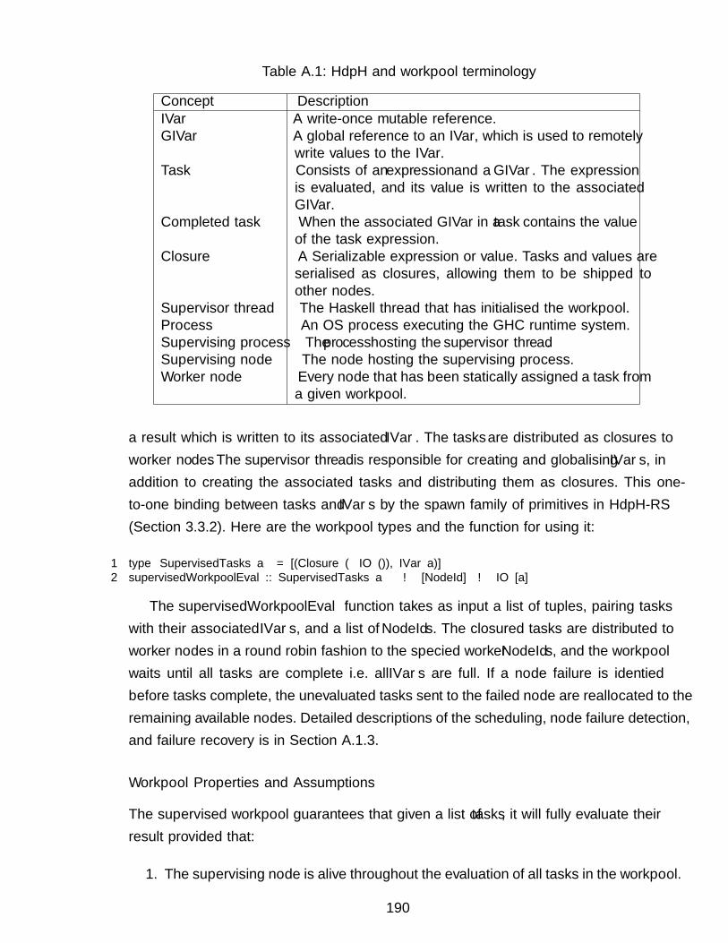
Table A.1: HdpH and workpool terminology

Concept DescriptionIVar A write-once mutable reference.GIVar A global reference to an IVar, which is used to remotely

write values to the IVar.Task Consists of an expression and a GIVar. The expression

is evaluated, and its value is written to the associatedGIVar.

Completed task When the associated GIVar in a task contains the valueof the task expression.

Closure A Serializable expression or value. Tasks and values areserialised as closures, allowing them to be shipped toother nodes.

Supervisor thread The Haskell thread that has initialised the workpool.Process An OS process executing the GHC runtime system.Supervising process The process hosting the supervisor thread.Supervising node The node hosting the supervising process.Worker node Every node that has been statically assigned a task from

a given workpool.

a result which is written to its associated IVar. The tasks are distributed as closures toworker nodes. The supervisor thread is responsible for creating and globalising IVars, inaddition to creating the associated tasks and distributing them as closures. This one-to-one binding between tasks and IVars by the spawn family of primitives in HdpH-RS(Section 3.3.2). Here are the workpool types and the function for using it:

1 type SupervisedTasks a = [(Closure (IO ()), IVar a)]2 supervisedWorkpoolEval :: SupervisedTasks a → [NodeId] → IO [a]

The supervisedWorkpoolEval function takes as input a list of tuples, pairing taskswith their associated IVars, and a list of NodeIds. The closured tasks are distributed toworker nodes in a round robin fashion to the specified worker NodeIds, and the workpoolwaits until all tasks are complete i.e. all IVars are full. If a node failure is identifiedbefore tasks complete, the unevaluated tasks sent to the failed node are reallocated to theremaining available nodes. Detailed descriptions of the scheduling, node failure detection,and failure recovery is in Section A.1.3.

Workpool Properties and Assumptions

The supervised workpool guarantees that given a list of tasks, it will fully evaluate theirresult provided that:

1. The supervising node is alive throughout the evaluation of all tasks in the workpool.

190

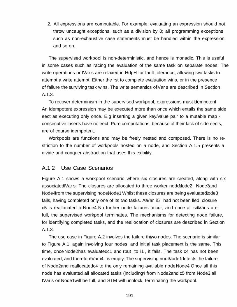
2. All expressions are computable. For example, evaluating an expression should notthrow uncaught exceptions, such as a division by 0; all programming exceptionssuch as non-exhaustive case statements must be handled within the expression;and so on.

The supervised workpool is non-deterministic, and hence is monadic. This is usefulin some cases such as racing the evaluation of the same task on separate nodes. Thewrite operations on IVars are relaxed in HdpH for fault tolerance, allowing two tasks toattempt a write attempt. Either the first to complete evaluation wins, or in the presenceof failure the surviving task wins. The write semantics of IVars are described in SectionA.1.3.

To recover determinism in the supervised workpool, expressions must be idempotent.An idempotent expression may be executed more than once which entails the same sideeffect as executing only once. E.g inserting a given key/value pair to a mutable map -consecutive inserts have no effect. Pure computations, because of their lack of side effects,are of course idempotent.

Workpools are functions and may be freely nested and composed. There is no re-striction to the number of workpools hosted on a node, and Section A.1.5 presents adivide-and-conquer abstraction that uses this flexibility.

A.1.2 Use Case Scenarios

Figure A.1 shows a workpool scenario where six closures are created, along with sixassociated IVars. The closures are allocated to three worker nodes: Node2, Node3 andNode4 from the supervising node, Node1. Whilst these closures are being evaluated, Node3fails, having completed only one of its two tasks. As IVar i5 had not been filled, closurec5 is reallocated to Node4. No further node failures occur, and once all six IVars arefull, the supervised workpool terminates. The mechanisms for detecting node failure,for identifying completed tasks, and the reallocation of closures are described in SectionA.1.3.

The use case in Figure A.2 involves the failure the two nodes. The scenario is similarto Figure A.1, again involving four nodes, and initial task placement is the same. Thistime, once Node2 has evaluated c1 and rput to i1, it fails. The task c4 has not beenevaluated, and therefore IVar i4 is empty. The supervising node Node1 detects the failureof Node2 and reallocated c4 to the only remaining available node, Node4. Once all thisnode has evaluated all allocated tasks (including c4 from Node2 and c5 from Node3, allIVars on Node1 will be full, and STM will unblock, terminating the workpool.

191

����������������

����

����������������

����

����

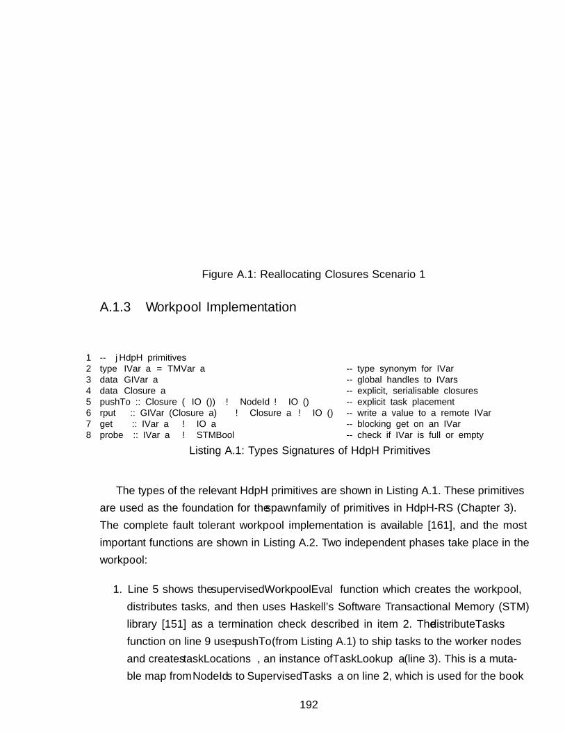
i1 i2 i3 i4 i5 i6 i1 i2 i3 i4 i5 i6

i1 i2 i3 i4 i5 i6

TaskLookup

TaskLookup

TaskLookup

Node 2

Node 3

Node 4

c1

c2

c3

c4

c5

c6

c2 c5 c2

pushTo pushTo pushTo pushTorput rput

Stage 1: Closures are distributed in a round robin fashion Stage 2: Node3 dies, closure 5 reallocated to Node4

c2

rput

Stage 3: Closure 5 evaluated; computation complete

c4c1

Node 2 Node 3

c6c3

Node 4

c4c1 c5 c3 c6

Node 2 Node 3 Node 4

IVars

IVars

IVars

Node 2

Node 3

Node 4

c1

c2

c3

c4

c6 c5

Node 2

Node 3

Node 4

c1

c2

c3

c4

c6 c5

c1 c4 c3 c6c5

Node 2 Node 3 Node 4

Node 1Node 1

Node 1

Figure A.1: Reallocating Closures Scenario 1

A.1.3 Workpool Implementation

1 -- |HdpH primitives2 type IVar a = TMVar a -- type synonym for IVar3 data GIVar a -- global handles to IVars4 data Closure a -- explicit, serialisable closures5 pushTo :: Closure (IO ()) → NodeId → IO () -- explicit task placement6 rput :: GIVar (Closure a) → Closure a → IO () -- write a value to a remote IVar7 get :: IVar a → IO a -- blocking get on an IVar8 probe :: IVar a → STM Bool -- check if IVar is full or empty

Listing A.1: Types Signatures of HdpH Primitives

The types of the relevant HdpH primitives are shown in Listing A.1. These primitivesare used as the foundation for the spawn family of primitives in HdpH-RS (Chapter 3).The complete fault tolerant workpool implementation is available [161], and the mostimportant functions are shown in Listing A.2. Two independent phases take place in theworkpool:

1. Line 5 shows the supervisedWorkpoolEval function which creates the workpool,distributes tasks, and then uses Haskell’s Software Transactional Memory (STM)library [151] as a termination check described in item 2. The distributeTasks

function on line 9 uses pushTo (from Listing A.1) to ship tasks to the worker nodesand creates taskLocations, an instance of TaskLookup a (line 3). This is a muta-ble map from NodeIds to SupervisedTasks a on line 2, which is used for the book

192

������������

����

������������

����

����������������

����

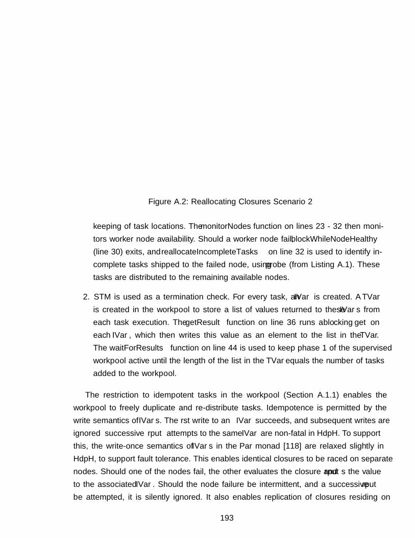
i1 i2 i3 i4 i5 i6

TaskLookup

TaskLookup

TaskLookup

TaskLookup

Node 2

Node 3

Node 4

c5

c4

c6c3

c2

c1

Node 2

Node 3

Node 4 c6c3

c2

c1

c5 c4

Node 2

Node 3

Node 4 c6c3

c2

c1

c5 c4

c6c3c4c1 c2 c5

pushTo

pushTo

pushTo

Stage 1: Closures are distributed in a round robin fashion

c2 c5

c6

c4

c2 c5 c3 c6c4c1

rput

pushTo

i1 i2 i3 i4 i5 i6

c2 c5

c6

c4

pushTo

i1 i2 i3 i4 i5 i6

rput

i1 i2 i3 i4 i5 i6

c1 c1

Stage 4: Closures 4 and 5 evaluated

Stage 2: Node3 dies, closure 5 reallocated to Node4

Stage 3: Node2 dies, closure 4 reallocated to Node4

rput

Node 2 Node 3 Node 4 Node 2 Node 3 Node 4

Node 1

Node 4Node 3Node 2Node 2 Node 3 Node 4

Node 1 Node 1

Node 1

IVars IVars

IVars IVars

c3 c3

Node 2

Node 3

Node 4

c4

c6c3

c2

c1

c5

Figure A.2: Reallocating Closures Scenario 2

keeping of task locations. The monitorNodes function on lines 23 - 32 then moni-tors worker node availability. Should a worker node fail, blockWhileNodeHealthy(line 30) exits, and reallocateIncompleteTasks on line 32 is used to identify in-complete tasks shipped to the failed node, using probe (from Listing A.1). Thesetasks are distributed to the remaining available nodes.

2. STM is used as a termination check. For every task, an IVar is created. A TVar

is created in the workpool to store a list of values returned to these IVars fromeach task execution. The getResult function on line 36 runs a blocking get oneach IVar, which then writes this value as an element to the list in the TVar.The waitForResults function on line 44 is used to keep phase 1 of the supervisedworkpool active until the length of the list in the TVar equals the number of tasksadded to the workpool.

The restriction to idempotent tasks in the workpool (Section A.1.1) enables theworkpool to freely duplicate and re-distribute tasks. Idempotence is permitted by thewrite semantics of IVars. The first write to an IVar succeeds, and subsequent writes areignored — successive rput attempts to the same IVar are non-fatal in HdpH. To supportthis, the write-once semantics of IVars in the Par monad [118] are relaxed slightly inHdpH, to support fault tolerance. This enables identical closures to be raced on separatenodes. Should one of the nodes fail, the other evaluates the closure and rputs the valueto the associated IVar. Should the node failure be intermittent, and a successive rput

be attempted, it is silently ignored. It also enables replication of closures residing on

193

1 -- |Workpool types2 type SupervisedTasks a = [(Closure (IO ()), IVar a)]3 type TaskLookup a = MVar (Map NodeId (SupervisedTasks a))45 supervisedWorkpoolEval :: SupervisedTasks a → [NodeId] → IO [a]6 supervisedWorkpoolEval tasks nodes = do7 -- PHASE 18 -- Ship the work, and create an instance of ’TaskLookup a’.9 taskLocations ← distributeTasks tasks nodes10 -- Monitor utilized nodes; reallocate incomplete tasks when worker nodes fail11 monitorNodes taskLocations1213 -- PHASE 214 -- Use STM as a termination check. Until all tasks are evaluated,15 -- phase 1 remains active.16 fullIvars ← newTVarIO []17 mapM_ (forkIO ◦ atomically ◦ getResult fullIvars ◦ snd) tasks18 results ← atomically $ waitForResults fullIvars (length tasks)1920 -- Finally, return the results of the tasks21 return results2223 monitorNodes :: TaskLookup a → IO ()24 monitorNodes taskLookup = do25 nodes ← fmap Map.keys $ readMVar taskLookup26 mapM_ (forkIO ◦ monitorNode) nodes27 where28 monitorNode :: NodeId → IO ()29 monitorNode node = do30 blockWhileNodeHealthy node -- Blocks while node is healthy (Used in Listing A.3)31 reallocateIncompleteTasks node taskLookup -- reallocate incomplete tasks32 -- shipped to ’node’3334 -- |Takes an IVar, runs a blocking ’get’ call, and writes35 -- the value to the list of values in a TVar36 getResult :: TVar [a] → IVar a → STM ()37 getResult values ivar = do38 v ← get ivar39 vs ← readTVar values40 writeTVar results (vs ++ [v])4142 -- |After each write to the TVar in ’evalTask’, the length of the list43 -- is checked. If it matches the number of tasks, STM releases the block.44 waitForResults :: TVar [a] → Int → STM [a]45 waitForResults values i = do46 vs ← readTVar values47 if length vs == i then return vs else retry

Listing A.2: Workpool Implementation and Use of STM as a Termination Check

overloaded nodes to be duplicated on to healthy nodes.It would be unnecessary and costly to reallocate tasks if they had been fully evaluated

prior to the failure of the worker node it was assigned to. For this purpose, the probe

194

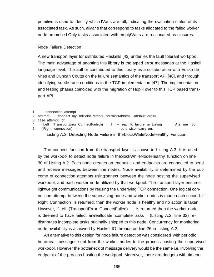
primitive is used to identify which IVars are full, indicating the evaluation status of itsassociated task. As such, all IVars that correspond to tasks allocated to the failed workernode are probed. Only tasks associated with empty IVars are reallocated as closures.

Node Failure Detection

A new transport layer for distributed Haskells [43] underlies the fault tolerant workpool.The main advantage of adopting this library is the typed error messages at the Haskelllanguage level. The author contributed to this library as a collaboration with Edsko deVries and Duncan Coutts on the failure semantics of the transport API [48], and throughidentifying subtle race conditions in the TCP implementation [47]. The implementationand testing phases coincided with the migration of HdpH over to this TCP based trans-port API.

1 -- connection attempt2 attempt ← connect myEndPoint remoteEndPointAddress <default args>3 case attempt of4 (Left (TransportError ConnectFailed)) → -- react to failure, in Listing A.2 line 305 (Right connection) → -- otherwise, carry on.

Listing A.3: Detecting Node Failure in the blockWhileNodeHealthy Function

The connect function from the transport layer is shown in Listing A.3. It is usedby the workpool to detect node failure in the blockWhileNodeHealthy function on line30 of Listing A.2. Each node creates an endpoint, and endpoints are connected to sendand receive messages between the nodes. Node availability is determined by the out-come of connection attempts using connect between the node hosting the supervisedworkpool, and each worker node utilized by that workpool. The transport layer ensureslightweight communications by reusing the underlying TCP connection. One logical con-nection attempt between the supervising node and worker nodes is made each second. IfRight Connection is returned, then the worker node is healthy and no action is taken.However, if Left (TransportError ConnectFailed) is returned then the worker nodeis deemed to have failed, and reallocateIncompleteTasks (Listing A.2, line 32) re-distributes incomplete tasks originally shipped to this node. Concurrency for monitoringnode availability is achieved by Haskell IO threads on line 26 in Listing A.2.

An alternative to this design for node failure detection was considered — with periodicheartbeat messages sent from the worker nodes to the process hosting the supervisedworkpool. However the bottleneck of message delivery would be the same i.e. involving theendpoint of the process hosting the workpool. Moreover, there are dangers with timeout

195

values for expecting heartbeat messages in asynchronous messaging systems such as theone employed by HdpH. Remote nodes may be wrongly judged to have failed e.g. whenthe message queue on the workpool process is flooded, and heartbeat messages are notpopped from the message queue within the timeout period. Our design avoids this dangerby synchronously checking each connection.

Each workpool hosted on a node must monitor the availability of worker nodes. Withnested or composed supervised workpools there is a risk that the network will be satu-rated with connect requests to monitor node availability. Our architecture avoids thisby creating just one Haskell thread per node that monitors availability of all other nodes,irrespective of the number of workpools hosted on a node. Each supervisor thread com-municates with these monitoring threads to identify node failure. See the complete im-plementation [161] for details.

A.1.4 Workpool Scheduling

One limitation of our supervised workpool is the naive scheduling of tasks between nodes.The strategy is simple — it eagerly distributes the tasks in the workpool between thenodes in a round robin fashion over the ordering of nodes allocated to the workpool.Recall the workpool primitive from Section A.1.1:

1 supervisedWorkpoolEval :: SupervisedTasks a → [NodeId] → IO [a]

It is up to the programmer to order the NodeIds in a sensible sequence. The orderingin the algorithmic skeletons in Section A.1.5 is sensitive to each skeleton. A suitable nodeorder must be selected for each of the skeletons in Section A.1.5. For example, the list ofnodes IDs passed to the parallel map are simply sorted in order, and then given to theworkpool. In the divide and conquer skeleton, the NodeIds are first of all randomised,and are then assigned to the workpool. This avoids overloading nodes near the head of asorted list of NodeIds.

The workpool is eager and preemptive in its scheduling. HdpH-RS has more sophis-ticated scheduling strategies than the workpool in this chapter, though the recovery andfailure detection techniques in HdpH-RS are heavily influenced by the workpool.

A.1.5 Workpool High Level Fault Tolerant Abstractions

It is straight forward to implement algorithmic skeletons in HdpH [114]. This present workextends these by adding resilience to the execution of two generic parallel algorithmicskeletons.

196

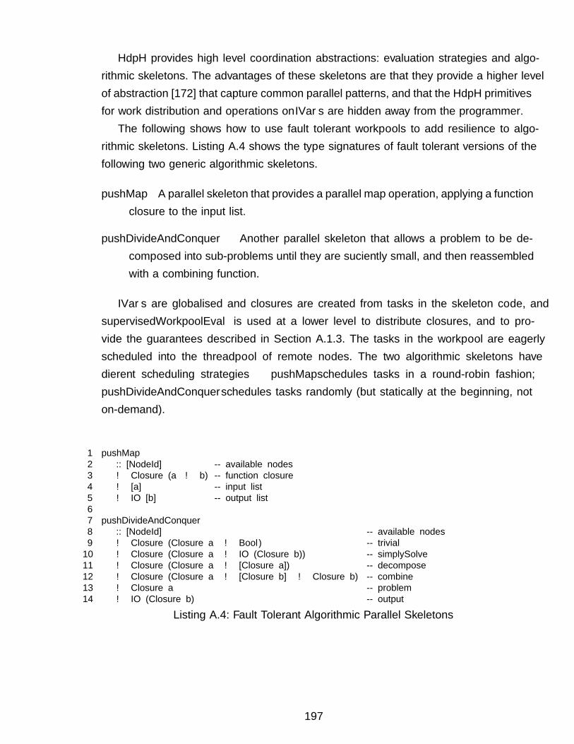
HdpH provides high level coordination abstractions: evaluation strategies and algo-rithmic skeletons. The advantages of these skeletons are that they provide a higher levelof abstraction [172] that capture common parallel patterns, and that the HdpH primitivesfor work distribution and operations on IVars are hidden away from the programmer.

The following shows how to use fault tolerant workpools to add resilience to algo-rithmic skeletons. Listing A.4 shows the type signatures of fault tolerant versions of thefollowing two generic algorithmic skeletons.

pushMap A parallel skeleton that provides a parallel map operation, applying a functionclosure to the input list.

pushDivideAndConquer Another parallel skeleton that allows a problem to be de-composed into sub-problems until they are sufficiently small, and then reassembledwith a combining function.

IVars are globalised and closures are created from tasks in the skeleton code, andsupervisedWorkpoolEval is used at a lower level to distribute closures, and to pro-vide the guarantees described in Section A.1.3. The tasks in the workpool are eagerlyscheduled into the threadpool of remote nodes. The two algorithmic skeletons havedifferent scheduling strategies — pushMap schedules tasks in a round-robin fashion;pushDivideAndConquer schedules tasks randomly (but statically at the beginning, noton-demand).

1 pushMap2 :: [NodeId] -- available nodes3 → Closure (a → b) -- function closure4 → [a] -- input list5 → IO [b] -- output list67 pushDivideAndConquer8 :: [NodeId] -- available nodes9 → Closure (Closure a → Bool) -- trivial10 → Closure (Closure a → IO (Closure b)) -- simplySolve11 → Closure (Closure a → [Closure a]) -- decompose12 → Closure (Closure a → [Closure b] → Closure b) -- combine13 → Closure a -- problem14 → IO (Closure b) -- output

Listing A.4: Fault Tolerant Algorithmic Parallel Skeletons

197

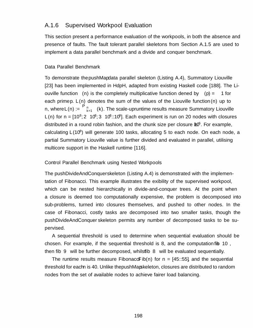
A.1.6 Supervised Workpool Evaluation

This section present a performance evaluation of the workpools, in both the absence andpresence of faults. The fault tolerant parallel skeletons from Section A.1.5 are used toimplement a data parallel benchmark and a divide and conquer benchmark.

Data Parallel Benchmark

To demonstrate the pushMap data parallel skeleton (Listing A.4), Summatory Liouville[23] has been implemented in HdpH, adapted from existing Haskell code [188]. The Li-ouville function λ(n) is the completely multiplicative function defined by λ(p) = −1 foreach prime p. L(n) denotes the sum of the values of the Liouville function λ(n) up ton, where L(n) := ∑n

k=1 λ(k). The scale-up runtime results measure Summatory LiouvilleL(n) for n = [108, 2 · 108, 3 · 108..109]. Each experiment is run on 20 nodes with closuresdistributed in a round robin fashion, and the chunk size per closure is 106. For example,calculating L(108) will generate 100 tasks, allocating 5 to each node. On each node, apartial Summatory Liouville value is further divided and evaluated in parallel, utilisingmulticore support in the Haskell runtime [116].

Control Parallel Benchmark using Nested Workpools

The pushDivideAndConquer skeleton (Listing A.4) is demonstrated with the implemen-tation of Fibonacci. This example illustrates the flexibility of the supervised workpool,which can be nested hierarchically in divide-and-conquer trees. At the point whena closure is deemed too computationally expensive, the problem is decomposed intosub-problems, turned into closures themselves, and pushed to other nodes. In thecase of Fibonacci, costly tasks are decomposed into two smaller tasks, though thepushDivideAndConquer skeleton permits any number of decomposed tasks to be su-pervised.

A sequential threshold is used to determine when sequential evaluation should bechosen. For example, if the sequential threshold is 8, and the computation is fib 10,then fib 9 will be further decomposed, whilst fib 8 will be evaluated sequentially.

The runtime results measure Fibonacci Fib(n) for n = [45..55], and the sequentialthreshold for each n is 40. Unlike the pushMap skeleton, closures are distributed to randomnodes from the set of available nodes to achieve fairer load balancing.

198

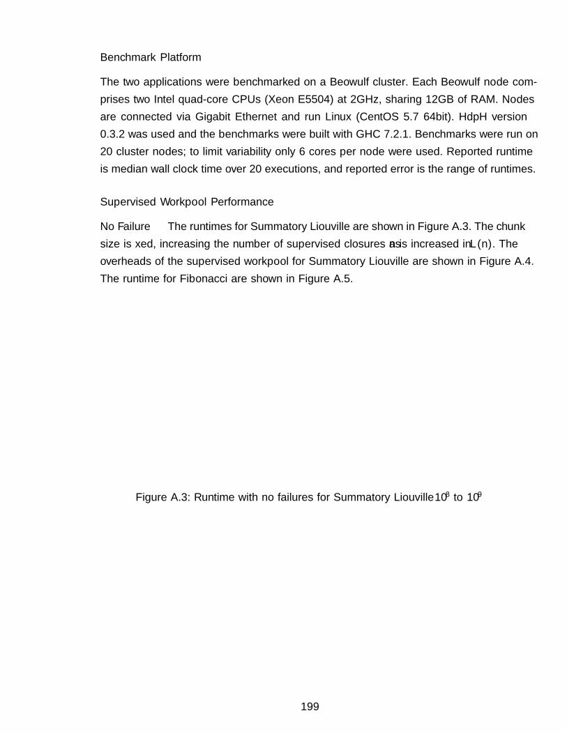
Benchmark Platform

The two applications were benchmarked on a Beowulf cluster. Each Beowulf node com-prises two Intel quad-core CPUs (Xeon E5504) at 2GHz, sharing 12GB of RAM. Nodesare connected via Gigabit Ethernet and run Linux (CentOS 5.7 64bit). HdpH version0.3.2 was used and the benchmarks were built with GHC 7.2.1. Benchmarks were run on20 cluster nodes; to limit variability only 6 cores per node were used. Reported runtimeis median wall clock time over 20 executions, and reported error is the range of runtimes.

Supervised Workpool Performance

No Failure The runtimes for Summatory Liouville are shown in Figure A.3. The chunksize is fixed, increasing the number of supervised closures as n is increased in L(n). Theoverheads of the supervised workpool for Summatory Liouville are shown in Figure A.4.The runtime for Fibonacci are shown in Figure A.5.

0

50

100

150

200

250

300

1e+08 2e+08 3e+08 4e+08 5e+08 6e+08 7e+08 8e+08 9e+08 1e+09

Run

time

(sec

onds

)

SummatoryLiouville(n)

Runtime Performance of Summatory LiovilleUsing supervision

No supervision

Figure A.3: Runtime with no failures for Summatory Liouville 108 to 109

199

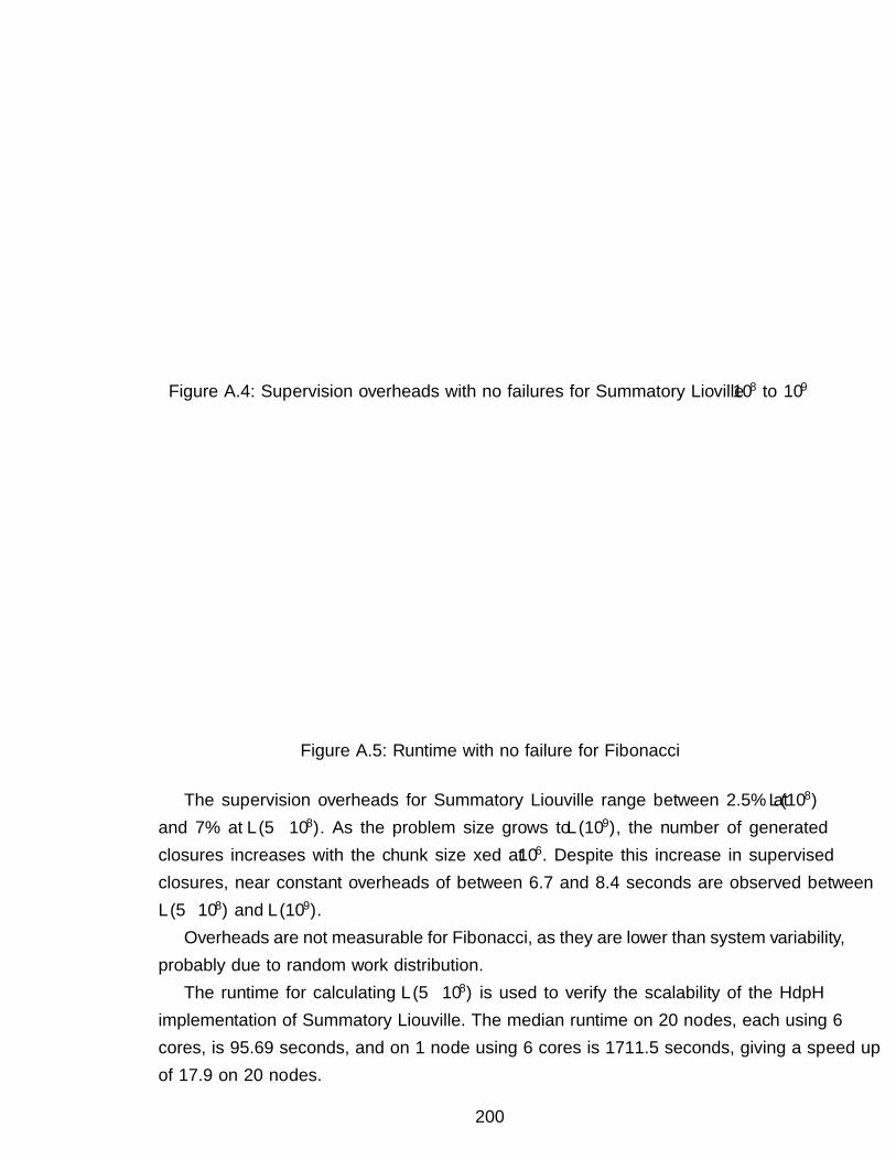
0

2

4

6

8

10

12

14

100 200 300 400 500 600 700 800 900 1000 0

1

2

3

4

5

6

7

8

Ove

rhea

d (s

econ

ds)

Ove

rhea

d (p

erce

ntag

e)

Number of closures supervised

Supervision Overheads in Summatory LiouvilleUsing supervision

No supervsionPercentage overhead

Figure A.4: Supervision overheads with no failures for Summatory Lioville 108 to 109

0

10

20

30

40

50

60

70

80

90

44 46 48 50 52 54 56

Run

time

(sec

onds

)

Fibonacci(n)

Fibonacci on 20 Nodes, 6 cores per node (no failures)

Using supervisionNo supervision

Figure A.5: Runtime with no failure for Fibonacci

The supervision overheads for Summatory Liouville range between 2.5% at L(108)and 7% at L(5 · 108). As the problem size grows to L(109), the number of generatedclosures increases with the chunk size fixed at 106. Despite this increase in supervisedclosures, near constant overheads of between 6.7 and 8.4 seconds are observed betweenL(5 · 108) and L(109).

Overheads are not measurable for Fibonacci, as they are lower than system variability,probably due to random work distribution.

The runtime for calculating L(5 · 108) is used to verify the scalability of the HdpHimplementation of Summatory Liouville. The median runtime on 20 nodes, each using 6cores, is 95.69 seconds, and on 1 node using 6 cores is 1711.5 seconds, giving a speed upof 17.9 on 20 nodes.

200

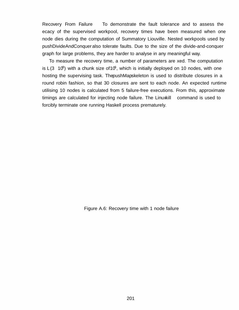
Recovery From Failure To demonstrate the fault tolerance and to assess theefficacy of the supervised workpool, recovery times have been measured when onenode dies during the computation of Summatory Liouville. Nested workpools used bypushDivideAndConquer also tolerate faults. Due to the size of the divide-and-conquergraph for large problems, they are harder to analyse in any meaningful way.

To measure the recovery time, a number of parameters are fixed. The computationis L(3 · 108) with a chunk size of 106, which is initially deployed on 10 nodes, with onehosting the supervising task. The pushMap skeleton is used to distribute closures in around robin fashion, so that 30 closures are sent to each node. An expected runtimeutilising 10 nodes is calculated from 5 failure-free executions. From this, approximatetimings are calculated for injecting node failure. The Linux kill command is used toforcibly terminate one running Haskell process prematurely.

90

95

100

105

110

115

120

0 % 20 % 40 % 60 % 80 % 100 %

Run

time

(Sec

onds

)

Time of Node Failure w.r.t. Estimated Runtime

Summatory Liouville Runtimes with 1 Node Failure

Mean of failure free runtimesRuntimes with failure

Using 9 nodes no failuresUsing 10 nodes no failures

Figure A.6: Recovery time with 1 node failure

201

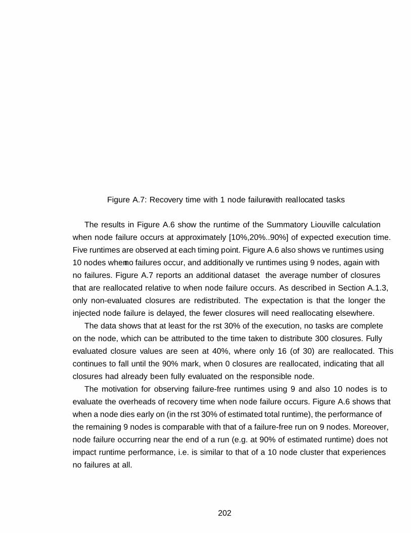
90

95

100

105

110

115

120

0 % 20 % 40 % 60 % 80 % 100 %

0

3

6

9

12

15

18

21

24

27

30

33

Run

time

(Sec

onds

)

Num

ber

of r

eallo

cate

d cl

osur

es

Time of Node Failure w.r.t. Estimated Runtime

Summatory Liouville Runtimes with 1 Node Failure

Mean closure reallocationMean of failure free runtimes

Runtimes with failureUsing 9 nodes no failures

Using 10 nodes no failures

Figure A.7: Recovery time with 1 node failure with reallocated tasks

The results in Figure A.6 show the runtime of the Summatory Liouville calculationwhen node failure occurs at approximately [10%,20%..90%] of expected execution time.Five runtimes are observed at each timing point. Figure A.6 also shows five runtimes using10 nodes when no failures occur, and additionally five runtimes using 9 nodes, again withno failures. Figure A.7 reports an additional dataset — the average number of closuresthat are reallocated relative to when node failure occurs. As described in Section A.1.3,only non-evaluated closures are redistributed. The expectation is that the longer theinjected node failure is delayed, the fewer closures will need reallocating elsewhere.

The data shows that at least for the first 30% of the execution, no tasks are completeon the node, which can be attributed to the time taken to distribute 300 closures. Fullyevaluated closure values are seen at 40%, where only 16 (of 30) are reallocated. Thiscontinues to fall until the 90% mark, when 0 closures are reallocated, indicating that allclosures had already been fully evaluated on the responsible node.

The motivation for observing failure-free runtimes using 9 and also 10 nodes is toevaluate the overheads of recovery time when node failure occurs. Figure A.6 shows thatwhen a node dies early on (in the first 30% of estimated total runtime), the performance ofthe remaining 9 nodes is comparable with that of a failure-free run on 9 nodes. Moreover,node failure occurring near the end of a run (e.g. at 90% of estimated runtime) does notimpact runtime performance, i.e. is similar to that of a 10 node cluster that experiencesno failures at all.

202

A.1.7 Summary

This chapter presents a language based approach to fault tolerant distributed-memoryparallel computation in Haskell: a fault tolerant workpool that hides task scheduling,failure detection and task replication from the programmer. Fault tolerant versions oftwo algorithmic skeletons are developed using the workpool. They provide high levelabstractions for fault tolerant parallel computation on distributed-memory architectures.To the best of the authors knowledge the supervised workpool is a novel construct.

The workpool and the skeletons guarantee the completion of tasks even in the presenceof multiple node failures, withstanding the failure of all but the supervising node. Thesupervised workpool has acceptable runtime overheads — between 2.5% and 7% using adata parallel skeleton. Moreover when a node fails, the recovery costs are negligible.

This marks the end of a feasibility study motivated by the claim that HdpH has thepotential for fault tolerance [114]. The limitations of the supervised workpools, describedin Section A.1.4, are that scheduling is preemptive and eager. There is no load balancing.The ideas of propagated fault detection from the transport layer, and freely replicatingidempotent tasks are taken forward into HdpH-RS in Chapter 3.

A.2 Programming with Futures

Programming with futures [95] is a simple programming abstraction for parallel schedul-ing. A future can be thought of as placeholder for a value that is set to contain a realvalue once that value becomes known, by evaluating the expression. Futures are createdwith the HdpH-RS spawn family of primitives (Section 3.3.2). Fault tolerant futures areimplemented with HdpH-RS using a modified version of IVars from HdpH, described inSection 5.1.1.

This section compares functional futures in monad-par [118], Erlang RPC [30], and theCloudHaskell Platform (CH-P) [181] with HdpH and HdpH-RS. It shows that HdpH-RS isthe only language that provides futures whilst supporting load balancing on distributed-memory architectures (Section A.2.1. It also highlights the inconsistencies between prim-itive naming conventions for programming with futures (Section A.2.2).

A.2.1 Library Support for Distributed Functional Futures

Table A.2 compares three features of monad-par, CH-P, HdpH and HdpH-RS.

1. Whether the runtime system for these languages balance load between the differentprocessing capabilities dynamically.

203

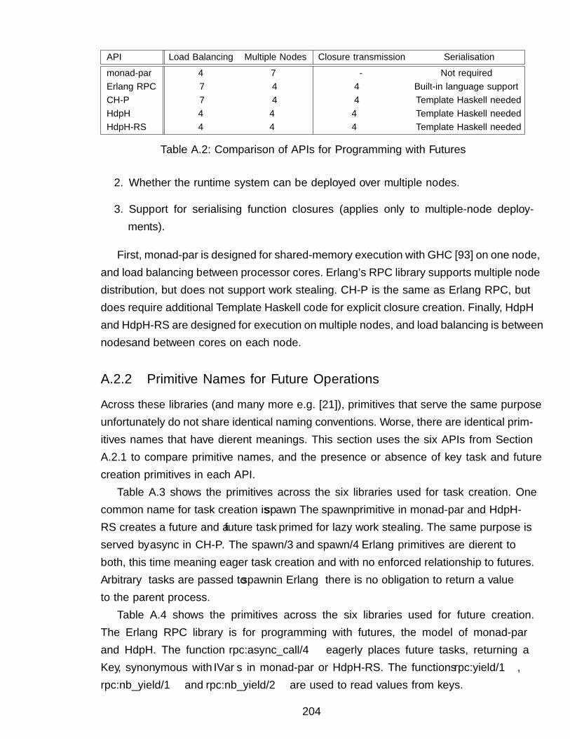
API Load Balancing Multiple Nodes Closure transmission Serialisation

monad-par 4 7 - Not requiredErlang RPC 7 4 4 Built-in language supportCH-P 7 4 4 Template Haskell neededHdpH 4 4 4 Template Haskell neededHdpH-RS 4 4 4 Template Haskell needed

Table A.2: Comparison of APIs for Programming with Futures

2. Whether the runtime system can be deployed over multiple nodes.

3. Support for serialising function closures (applies only to multiple-node deploy-ments).

First, monad-par is designed for shared-memory execution with GHC [93] on one node,and load balancing between processor cores. Erlang’s RPC library supports multiple nodedistribution, but does not support work stealing. CH-P is the same as Erlang RPC, butdoes require additional Template Haskell code for explicit closure creation. Finally, HdpHand HdpH-RS are designed for execution on multiple nodes, and load balancing is betweennodes and between cores on each node.

A.2.2 Primitive Names for Future Operations

Across these libraries (and many more e.g. [21]), primitives that serve the same purposeunfortunately do not share identical naming conventions. Worse, there are identical prim-itives names that have different meanings. This section uses the six APIs from SectionA.2.1 to compare primitive names, and the presence or absence of key task and futurecreation primitives in each API.

Table A.3 shows the primitives across the six libraries used for task creation. Onecommon name for task creation is spawn. The spawn primitive in monad-par and HdpH-RS creates a future and a future task primed for lazy work stealing. The same purpose isserved by async in CH-P. The spawn/3 and spawn/4 Erlang primitives are different toboth, this time meaning eager task creation and with no enforced relationship to futures.Arbitrary tasks are passed to spawn in Erlang — there is no obligation to return a valueto the parent process.

Table A.4 shows the primitives across the six libraries used for future creation.The Erlang RPC library is for programming with futures, the model of monad-parand HdpH. The function rpc:async_call/4 eagerly places future tasks, returning aKey, synonymous with IVars in monad-par or HdpH-RS. The functions rpc:yield/1,rpc:nb_yield/1 and rpc:nb_yield/2 are used to read values from keys.

204

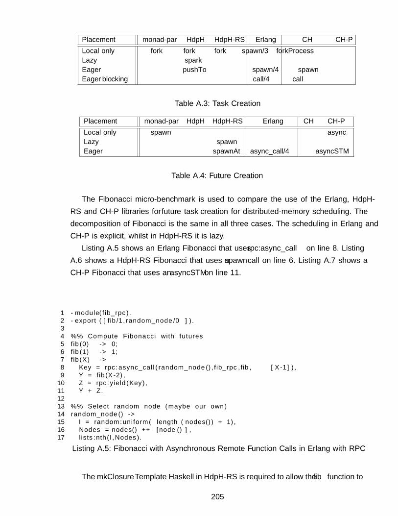
Placement monad-par HdpH HdpH-RS Erlang CH CH-PLocal only fork fork fork spawn/3 forkProcessLazy sparkEager pushTo spawn/4 spawnEager blocking call/4 call

Table A.3: Task Creation

Placement monad-par HdpH HdpH-RS Erlang CH CH-PLocal only spawn asyncLazy spawnEager spawnAt async_call/4 asyncSTM

Table A.4: Future Creation

The Fibonacci micro-benchmark is used to compare the use of the Erlang, HdpH-RS and CH-P libraries for future task creation for distributed-memory scheduling. Thedecomposition of Fibonacci is the same in all three cases. The scheduling in Erlang andCH-P is explicit, whilst in HdpH-RS it is lazy.

Listing A.5 shows an Erlang Fibonacci that uses rpc:async_call on line 8. ListingA.6 shows a HdpH-RS Fibonacci that uses a spawn call on line 6. Listing A.7 shows aCH-P Fibonacci that uses an asyncSTM on line 11.

1 -module(fib_rpc).2 -export([fib/1, random_node /0]).34 %% Compute Fibonacci with futures5 fib (0) -> 0;6 fib (1) -> 1;7 fib(X) ->8 Key = rpc:async_call(random_node (),fib_rpc ,fib ,[X-1]),9 Y = fib(X-2),10 Z = rpc:yield(Key),11 Y + Z.1213 %% Select random node (maybe our own)14 random_node () ->15 I = random:uniform(length(nodes ()) + 1),16 Nodes = nodes () ++ [node()],17 lists:nth(I,Nodes).

Listing A.5: Fibonacci with Asynchronous Remote Function Calls in Erlang with RPC

The mkClosure Template Haskell in HdpH-RS is required to allow the fib function to

205

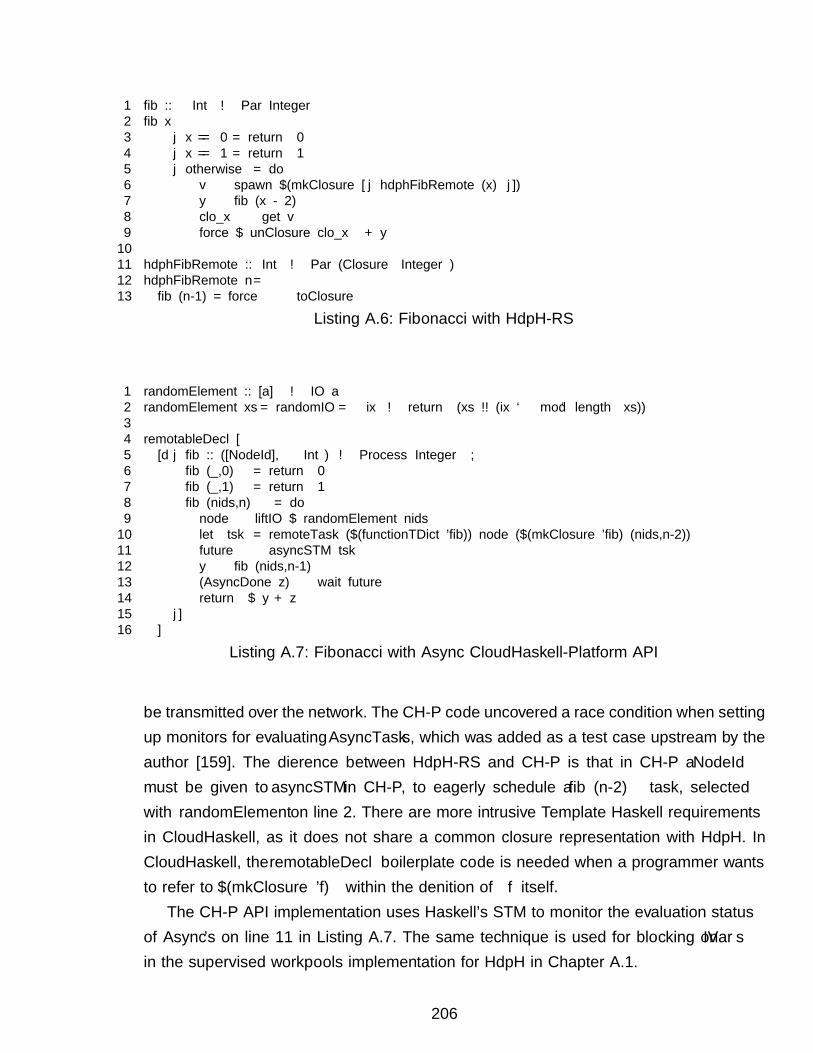
1 fib :: Int → Par Integer2 fib x3 | x == 0 = return 04 | x == 1 = return 15 | otherwise = do6 v ← spawn $(mkClosure [ | hdphFibRemote (x) |])7 y ← fib (x - 2)8 clo_x ← get v9 force $ unClosure clo_x + y1011 hdphFibRemote :: Int → Par (Closure Integer)12 hdphFibRemote n =13 fib (n-1) »= force ◦ toClosure

Listing A.6: Fibonacci with HdpH-RS

1 randomElement :: [a] → IO a2 randomElement xs = randomIO »= λix → return (xs !! (ix ‘mod‘ length xs))34 remotableDecl [5 [d | fib :: ([NodeId],Int) → Process Integer ;6 fib (_,0) = return 07 fib (_,1) = return 18 fib (nids,n) = do9 node ← liftIO $ randomElement nids10 let tsk = remoteTask ($(functionTDict ’fib)) node ($(mkClosure ’fib) (nids,n-2))11 future ← asyncSTM tsk12 y ← fib (nids,n-1)13 (AsyncDone z) ← wait future14 return $ y + z15 |]16 ]

Listing A.7: Fibonacci with Async CloudHaskell-Platform API

be transmitted over the network. The CH-P code uncovered a race condition when settingup monitors for evaluating AsyncTasks, which was added as a test case upstream by theauthor [159]. The difference between HdpH-RS and CH-P is that in CH-P a NodeId

must be given to asyncSTM in CH-P, to eagerly schedule a fib (n-2) task, selectedwith randomElement on line 2. There are more intrusive Template Haskell requirementsin CloudHaskell, as it does not share a common closure representation with HdpH. InCloudHaskell, the remotableDecl boilerplate code is needed when a programmer wantsto refer to $(mkClosure ’f) within the definition of f itself.

The CH-P API implementation uses Haskell’s STM to monitor the evaluation statusof Async’s on line 11 in Listing A.7. The same technique is used for blocking on IVarsin the supervised workpools implementation for HdpH in Chapter A.1.

206

monad-par HdpH HdpH-RS Erlang CH CH-PBlocking read get get get yield/1 waitNon-blocking read tryGet tryGet nb_yield/1 pollTimeout read nb_yield/2 waitTimeoutCheck fullness probe probe check

Table A.5: Operations on Futures

It is a similar story for operations on futures. In HdpH and HdpH-RS, a blocking waiton a future is get, which is also true for monad-par. In Erlang RPC it is rpc:yield/4,and in CH-P it is wait. The non-blocking version in HdpH and HdpH-RS is tryGet, inErlang RPC it is rpc:nb_yield/4 and in CH-P it is waitTimeout. The operations onfutures are shown in Table A.5.

This section has expanded on the introduction of the spawn family in Section 3.3.2. Itshows that HdpH balances load between processing elements. In contrast to the monad-par library which defines single-node multicores as a processing element, HdpH usesdistributed-memory multicore as processing elements. Moreover, HdpH-RS shares thefutures programming model with the Erlang RPC library and the CloudHaskell Plat-form on distributed-memory. Only the HdpH-RS runtime supports load-balancing forevaluating futures.

The second distinction in this section is the naming conventions for creating futures.The spawn convention in HdpH-RS was influenced by the monad-par API. It also usesIVars as futures. As HdpH was designed as a distributed-memory extension of this library,the spawn name is shared. In contrast, the CloudHaskell Platform primitive for eager taskplacement is asyncSTM. The Erlang primitive for eager task placement is async_call/4.The spawn and supervisedSpawn HdpH-RS primitives are unique in their function, inthis comparison of three functional libraries. They are used to create supervised sparksthat are lazily scheduled with load balancing on distributed-memory.

A.3 Promela Model Implementation

The Promela model used in Chapter 4 is in Listing A.8.

1 mtype = {FISH,DEADNODE,SCHEDULE,REQ,AUTH,DENIED,ACK,NOWORK,OBSOLETE,RESULT};2 mtype = {ONNODE,INTRANSITION};34 typedef Location5 {6 int from;7 int to;8 int at=3;9 }

207

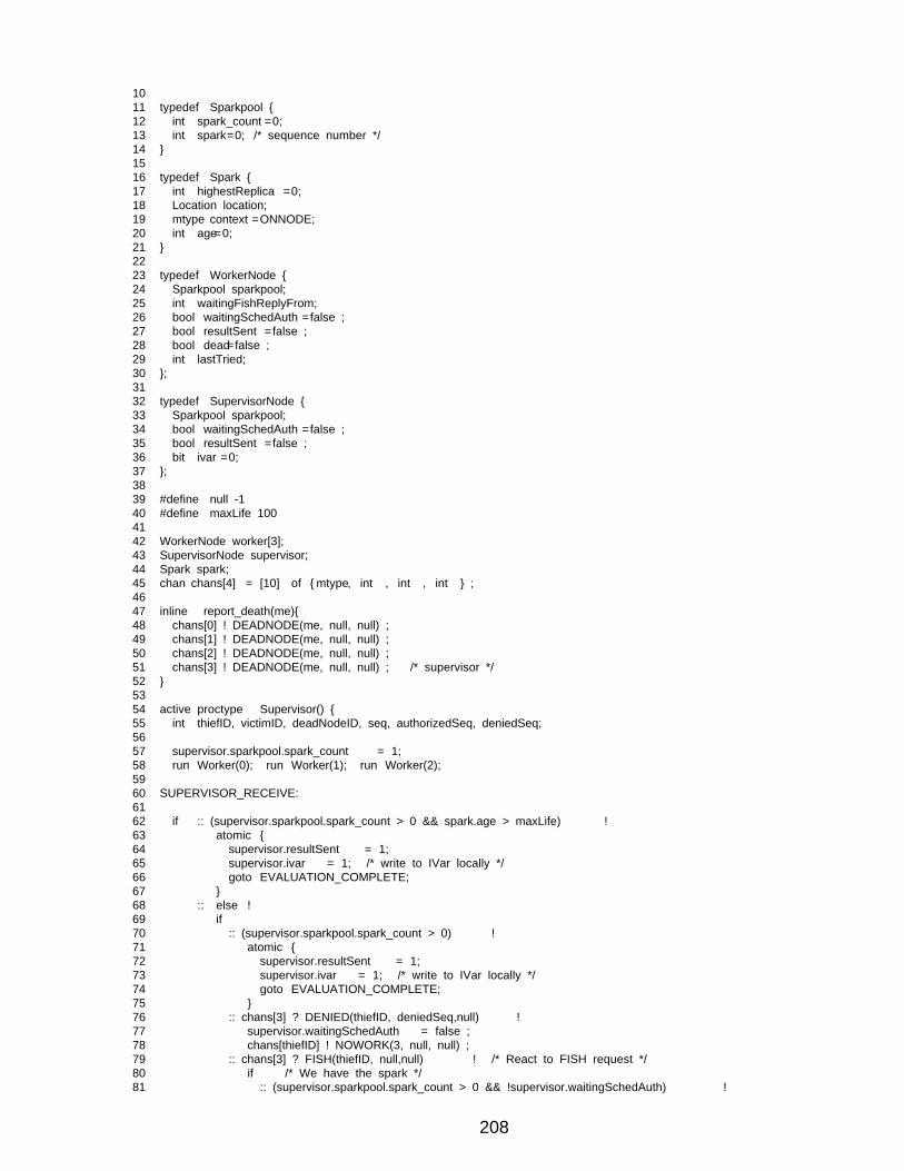
1011 typedef Sparkpool {12 int spark_count=0;13 int spark=0; /* sequence number */14 }1516 typedef Spark {17 int highestReplica=0;18 Location location;19 mtype context=ONNODE;20 int age=0;21 }2223 typedef WorkerNode {24 Sparkpool sparkpool;25 int waitingFishReplyFrom;26 bool waitingSchedAuth=false;27 bool resultSent=false;28 bool dead=false;29 int lastTried;30 };3132 typedef SupervisorNode {33 Sparkpool sparkpool;34 bool waitingSchedAuth=false;35 bool resultSent=false;36 bit ivar=0;37 };3839 #define null -140 #define maxLife 1004142 WorkerNode worker[3];43 SupervisorNode supervisor;44 Spark spark;45 chan chans[4] = [10] of {mtype, int , int , int } ;4647 inline report_death(me){48 chans[0] ! DEADNODE(me, null, null) ;49 chans[1] ! DEADNODE(me, null, null) ;50 chans[2] ! DEADNODE(me, null, null) ;51 chans[3] ! DEADNODE(me, null, null) ; /* supervisor */52 }5354 active proctype Supervisor() {55 int thiefID, victimID, deadNodeID, seq, authorizedSeq, deniedSeq;5657 supervisor.sparkpool.spark_count = 1;58 run Worker(0); run Worker(1); run Worker(2);5960 SUPERVISOR_RECEIVE:6162 if :: (supervisor.sparkpool.spark_count > 0 && spark.age > maxLife) →63 atomic {64 supervisor.resultSent = 1;65 supervisor.ivar = 1; /* write to IVar locally */66 goto EVALUATION_COMPLETE;67 }68 :: else →69 if70 :: (supervisor.sparkpool.spark_count > 0) →71 atomic {72 supervisor.resultSent = 1;73 supervisor.ivar = 1; /* write to IVar locally */74 goto EVALUATION_COMPLETE;75 }76 :: chans[3] ? DENIED(thiefID, deniedSeq,null) →77 supervisor.waitingSchedAuth = false;78 chans[thiefID] ! NOWORK(3, null, null) ;79 :: chans[3] ? FISH(thiefID, null,null) → /* React to FISH request */80 if /* We have the spark */81 :: (supervisor.sparkpool.spark_count > 0 && !supervisor.waitingSchedAuth) →

208

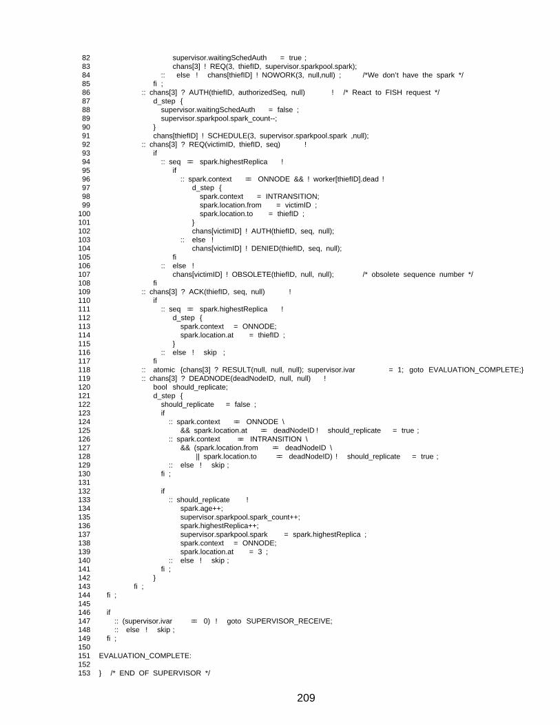
82 supervisor.waitingSchedAuth = true;83 chans[3] ! REQ(3, thiefID, supervisor.sparkpool.spark);84 :: else → chans[thiefID] ! NOWORK(3, null,null) ; /*We don’t have the spark */85 fi;86 :: chans[3] ? AUTH(thiefID, authorizedSeq, null) → /* React to FISH request */87 d_step {88 supervisor.waitingSchedAuth = false;89 supervisor.sparkpool.spark_count--;90 }91 chans[thiefID] ! SCHEDULE(3, supervisor.sparkpool.spark ,null);92 :: chans[3] ? REQ(victimID, thiefID, seq) →93 if94 :: seq == spark.highestReplica →95 if96 :: spark.context == ONNODE && ! worker[thiefID].dead→97 d_step {98 spark.context = INTRANSITION;99 spark.location.from = victimID ;

100 spark.location.to = thiefID ;101 }102 chans[victimID] ! AUTH(thiefID, seq, null);103 :: else →104 chans[victimID] ! DENIED(thiefID, seq, null);105 fi106 :: else →107 chans[victimID] ! OBSOLETE(thiefID, null, null); /* obsolete sequence number */108 fi109 :: chans[3] ? ACK(thiefID, seq, null) →110 if111 :: seq == spark.highestReplica →112 d_step {113 spark.context = ONNODE;114 spark.location.at = thiefID ;115 }116 :: else → skip ;117 fi118 :: atomic {chans[3] ? RESULT(null, null, null); supervisor.ivar = 1; goto EVALUATION_COMPLETE;}119 :: chans[3] ? DEADNODE(deadNodeID, null, null) →120 bool should_replicate;121 d_step {122 should_replicate = false;123 if124 :: spark.context == ONNODE \125 && spark.location.at == deadNodeID → should_replicate = true;126 :: spark.context == INTRANSITION \127 && (spark.location.from == deadNodeID \128 || spark.location.to == deadNodeID) → should_replicate = true;129 :: else → skip;130 fi;131132 if133 :: should_replicate →134 spark.age++;135 supervisor.sparkpool.spark_count++;136 spark.highestReplica++;137 supervisor.sparkpool.spark = spark.highestReplica ;138 spark.context = ONNODE;139 spark.location.at = 3 ;140 :: else → skip;141 fi;142 }143 fi;144 fi;145146 if147 :: (supervisor.ivar == 0) → goto SUPERVISOR_RECEIVE;148 :: else → skip;149 fi;150151 EVALUATION_COMPLETE:152153 } /* END OF SUPERVISOR */

209

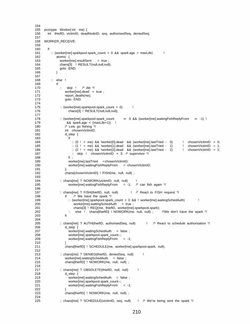
154155 proctype Worker(int me) {156 int thiefID, victimID, deadNodeID, seq, authorisedSeq, deniedSeq;157158 WORKER_RECEIVE:159160 if161 :: (worker[me].sparkpool.spark_count > 0 && spark.age > maxLife) →162 atomic {163 worker[me].resultSent = true;164 chans[3] ! RESULT(null,null,null);165 goto END;166 }167168 :: else →169 if170 :: skip → /* die */171 worker[me].dead = true;172 report_death(me);173 goto END;174175 :: (worker[me].sparkpool.spark_count > 0) →176 chans[3] ! RESULT(null,null,null);177178 :: (worker[me].sparkpool.spark_count == 0 && (worker[me].waitingFishReplyFrom == -1) \179 && spark.age < (maxLife+1)) →180 /* Lets go fishing */181 int chosenVictimID;182 d_step {183 if184 :: (0 != me) && !worker[0].dead && (worker[me].lastTried - 0) → chosenVictimID = 0;185 :: (1 != me) && !worker[1].dead && (worker[me].lastTried - 1) → chosenVictimID = 1;186 :: (2 != me) && !worker[2].dead && (worker[me].lastTried - 2) → chosenVictimID = 2;187 :: skip → chosenVictimID = 3; /* supervisor */188 fi;189 worker[me].lastTried=chosenVictimID;190 worker[me].waitingFishReplyFrom = chosenVictimID;191 };192 chans[chosenVictimID] ! FISH(me, null, null) ;193194 :: chans[me] ? NOWORK(victimID, null, null) →195 worker[me].waitingFishReplyFrom = -1; /* can fish again */196197 :: chans[me] ? FISH(thiefID, null, null) → /* React to FISH request */198 if /* We have the spark */199 :: (worker[me].sparkpool.spark_count > 0 && ! worker[me].waitingSchedAuth) →200 worker[me].waitingSchedAuth = true;201 chans[3] ! REQ(me, thiefID, worker[me].sparkpool.spark);202 :: else → chans[thiefID] ! NOWORK(me, null, null) ; /*We don’t have the spark */203 fi204205 :: chans[me] ? AUTH(thiefID, authorisedSeq, null) → /* React to schedule authorisation */206 d_step {207 worker[me].waitingSchedAuth = false;208 worker[me].sparkpool.spark_count--;209 worker[me].waitingFishReplyFrom = -1;210 }211 chans[thiefID] ! SCHEDULE(me, worker[me].sparkpool.spark, null);212213 :: chans[me] ? DENIED(thiefID, deniedSeq, null) →214 worker[me].waitingSchedAuth = false;215 chans[thiefID] ! NOWORK(me, null, null) ;216217 :: chans[me] ? OBSOLETE(thiefID, null, null) →218 d_step {219 worker[me].waitingSchedAuth = false;220 worker[me].sparkpool.spark_count--;221 worker[me].waitingFishReplyFrom = -1;222 }223 chans[thiefID] ! NOWORK(me, null, null) ;224225 :: chans[me] ? SCHEDULE(victimID, seq, null) → /* We’re being sent the spark */

210

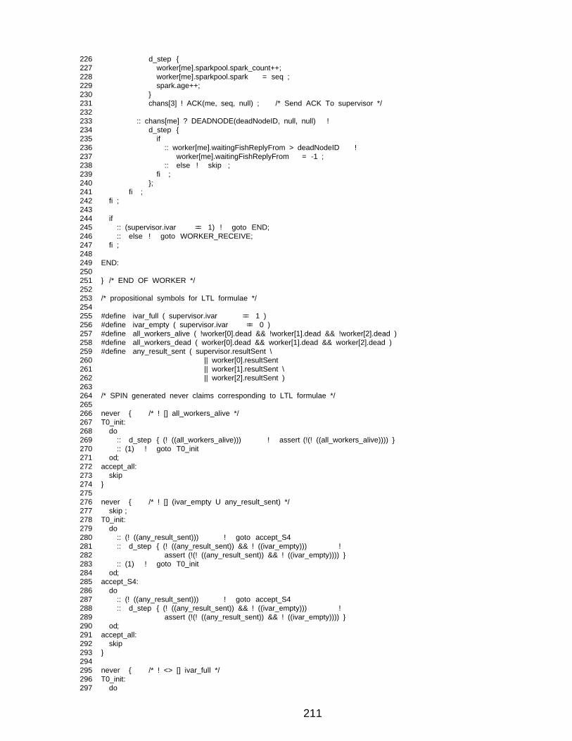
226 d_step {227 worker[me].sparkpool.spark_count++;228 worker[me].sparkpool.spark = seq ;229 spark.age++;230 }231 chans[3] ! ACK(me, seq, null) ; /* Send ACK To supervisor */232233 :: chans[me] ? DEADNODE(deadNodeID, null, null) →234 d_step {235 if236 :: worker[me].waitingFishReplyFrom > deadNodeID →237 worker[me].waitingFishReplyFrom = -1 ;238 :: else → skip ;239 fi ;240 };241 fi ;242 fi;243244 if245 :: (supervisor.ivar == 1) → goto END;246 :: else → goto WORKER_RECEIVE;247 fi;248249 END:250251 } /* END OF WORKER */252253 /* propositional symbols for LTL formulae */254255 #define ivar_full ( supervisor.ivar == 1 )256 #define ivar_empty ( supervisor.ivar == 0 )257 #define all_workers_alive ( !worker[0].dead && !worker[1].dead && !worker[2].dead )258 #define all_workers_dead ( worker[0].dead && worker[1].dead && worker[2].dead )259 #define any_result_sent ( supervisor.resultSent \260 || worker[0].resultSent261 || worker[1].resultSent \262 || worker[2].resultSent )263264 /* SPIN generated never claims corresponding to LTL formulae */265266 never { /* ! [] all_workers_alive */267 T0_init:268 do269 :: d_step { (! ((all_workers_alive))) → assert(!(! ((all_workers_alive)))) }270 :: (1) → goto T0_init271 od;272 accept_all:273 skip274 }275276 never { /* ! [] (ivar_empty U any_result_sent) */277 skip;278 T0_init:279 do280 :: (! ((any_result_sent))) → goto accept_S4281 :: d_step { (! ((any_result_sent)) && ! ((ivar_empty))) →282 assert(!(! ((any_result_sent)) && ! ((ivar_empty)))) }283 :: (1) → goto T0_init284 od;285 accept_S4:286 do287 :: (! ((any_result_sent))) → goto accept_S4288 :: d_step { (! ((any_result_sent)) && ! ((ivar_empty))) →289 assert(!(! ((any_result_sent)) && ! ((ivar_empty)))) }290 od;291 accept_all:292 skip293 }294295 never { /* ! <> [] ivar_full */296 T0_init:297 do

211

298 :: (! ((ivar_full))) → goto accept_S9299 :: (1) → goto T0_init300 od;301 accept_S9:302 do303 :: (1) → goto T0_init304 od;305 }

Listing A.8: Promela Model of HdpH-RS Scheduler

A.4 Feeding Promela Bug Fix to Implementation

This section shows the Promela fix (Section A.4.1) and Haskell fix (Section A.4.2) to thescheduling bug described in Section 4.6.

A.4.1 Bug Fix in Promela Model

commit 7 f23a46035cbb9a12aeadb84ab8dbcb0c28e7a48

Author : Rob Stewart <robstewart57@gmail .com >

Date: Thu Jun 27 23:21:20 2013 +0100

Additional condition when supervisor receives REQ.

Now the supervisor checks that the thief in a REQ message is still

alive before it authorises with the scheduling with AUTH. This has

been fed back in to the HdpH -RS implementation git commit

d2c5c7e58257ae11443c00203a9cc984b13601ad

diff --git a/ spin_models / hdph_scheduler .pml b/ spin_models / hdph_scheduler .pml

index 3 bb033f .. e94ce63 100644

--- a/ spin_models / hdph_scheduler .pml

+++ b/ spin_models / hdph_scheduler .pml

:: chans [3] ? REQ( sendingNode , fishingNodeID , seq) ->

if

:: seq == spark . highestReplica ->

if

- :: spark . context == ONNODE ->

+ :: spark . context == ONNODE && ! worker [ fishingNodeID ]. dead ->

atomic {

spark . context = INTRANSITION ;

spark . location .from = sendingNode ;

spark . location .to = worker [ fishingNodeID ]. inChan ;

}

sendingNode ! AUTH( worker [ fishingNodeID ]. inChan , seq );

:: else ->

sendingNode ! DENIED ( worker [ fishingNodeID ]. inChan , seq );

A.4.2 Bug Fix in Haskell

commit d2c5c7e58257ae11443c00203a9cc984b13601ad

Author : Rob Stewart <robstewart57@gmail .com >

212

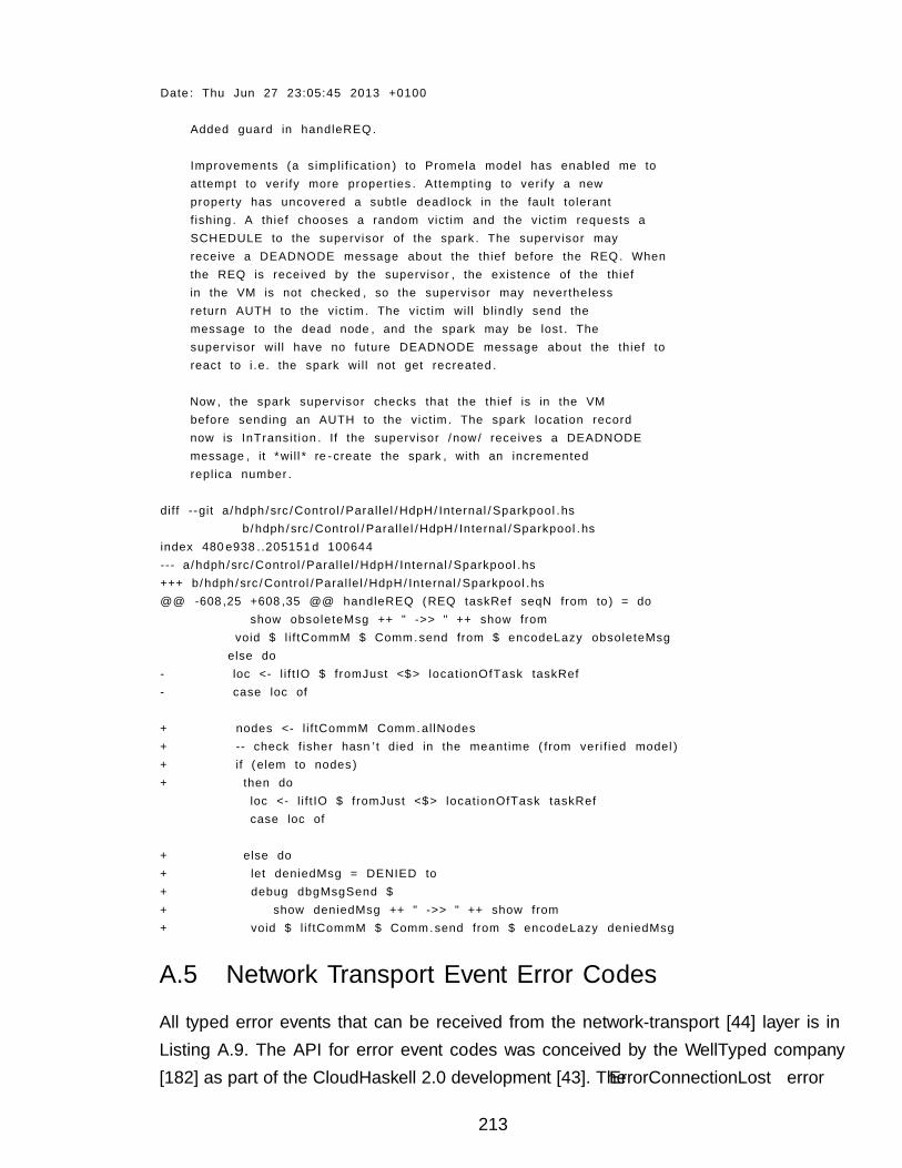
Date: Thu Jun 27 23:05:45 2013 +0100

Added guard in handleREQ .

Improvements (a simplification ) to Promela model has enabled me to

attempt to verify more properties . Attempting to verify a new

property has uncovered a subtle deadlock in the fault tolerant

fishing . A thief chooses a random victim and the victim requests a

SCHEDULE to the supervisor of the spark . The supervisor may

receive a DEADNODE message about the thief before the REQ. When

the REQ is received by the supervisor , the existence of the thief

in the VM is not checked , so the supervisor may nevertheless

return AUTH to the victim . The victim will blindly send the

message to the dead node , and the spark may be lost. The

supervisor will have no future DEADNODE message about the thief to

react to i.e. the spark will not get recreated .

Now , the spark supervisor checks that the thief is in the VM

before sending an AUTH to the victim . The spark location record

now is InTransition . If the supervisor /now/ receives a DEADNODE

message , it *will* re - create the spark , with an incremented

replica number .

diff --git a/hdph/src/ Control / Parallel /HdpH/ Internal / Sparkpool .hs

b/hdph/src/ Control / Parallel /HdpH/ Internal / Sparkpool .hs

index 480 e938 ..205151 d 100644

--- a/hdph/src/ Control / Parallel /HdpH/ Internal / Sparkpool .hs

+++ b/hdph/src/ Control / Parallel /HdpH/ Internal / Sparkpool .hs

@@ -608 ,25 +608 ,35 @@ handleREQ (REQ taskRef seqN from to) = do

show obsoleteMsg ++ " ->> " ++ show from

void $ liftCommM $ Comm.send from $ encodeLazy obsoleteMsg

else do

- loc <- liftIO $ fromJust <$> locationOfTask taskRef

- case loc of

+ nodes <- liftCommM Comm. allNodes

+ -- check fisher hasn ’t died in the meantime (from verified model )

+ if (elem to nodes )

+ then do

loc <- liftIO $ fromJust <$> locationOfTask taskRef

case loc of

+ else do

+ let deniedMsg = DENIED to

+ debug dbgMsgSend $

+ show deniedMsg ++ " ->> " ++ show from

+ void $ liftCommM $ Comm.send from $ encodeLazy deniedMsg

A.5 Network Transport Event Error Codes

All typed error events that can be received from the network-transport [44] layer is inListing A.9. The API for error event codes was conceived by the WellTyped company[182] as part of the CloudHaskell 2.0 development [43]. The ErrorConnectionLost error

213

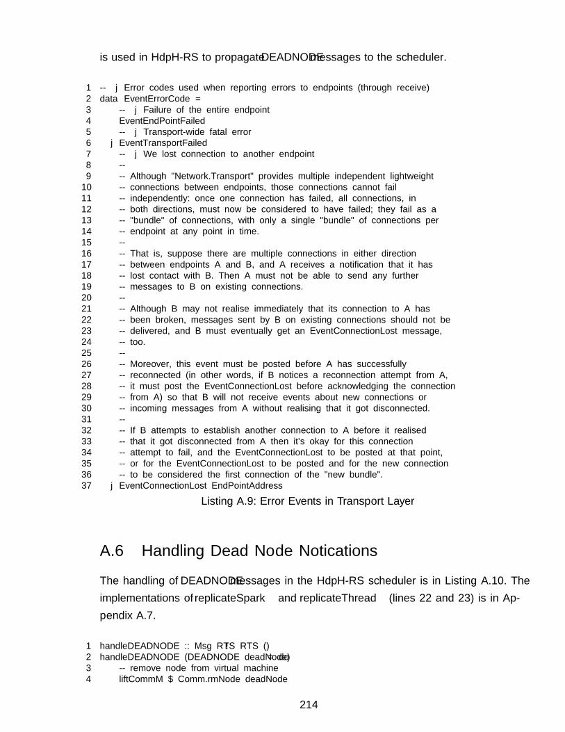
is used in HdpH-RS to propagate DEADNODE messages to the scheduler.

1 -- | Error codes used when reporting errors to endpoints (through receive)2 data EventErrorCode =3 -- | Failure of the entire endpoint4 EventEndPointFailed5 -- | Transport-wide fatal error6 | EventTransportFailed7 -- | We lost connection to another endpoint8 --9 -- Although "Network.Transport" provides multiple independent lightweight10 -- connections between endpoints, those connections cannot fail11 -- independently: once one connection has failed, all connections, in12 -- both directions, must now be considered to have failed; they fail as a13 -- "bundle" of connections, with only a single "bundle" of connections per14 -- endpoint at any point in time.15 --16 -- That is, suppose there are multiple connections in either direction17 -- between endpoints A and B, and A receives a notification that it has18 -- lost contact with B. Then A must not be able to send any further19 -- messages to B on existing connections.20 --21 -- Although B may not realise immediately that its connection to A has22 -- been broken, messages sent by B on existing connections should not be23 -- delivered, and B must eventually get an EventConnectionLost message,24 -- too.25 --26 -- Moreover, this event must be posted before A has successfully27 -- reconnected (in other words, if B notices a reconnection attempt from A,28 -- it must post the EventConnectionLost before acknowledging the connection29 -- from A) so that B will not receive events about new connections or30 -- incoming messages from A without realising that it got disconnected.31 --32 -- If B attempts to establish another connection to A before it realised33 -- that it got disconnected from A then it’s okay for this connection34 -- attempt to fail, and the EventConnectionLost to be posted at that point,35 -- or for the EventConnectionLost to be posted and for the new connection36 -- to be considered the first connection of the "new bundle".37 | EventConnectionLost EndPointAddress

Listing A.9: Error Events in Transport Layer

A.6 Handling Dead Node Notifications

The handling of DEADNODE messages in the HdpH-RS scheduler is in Listing A.10. Theimplementations of replicateSpark and replicateThread (lines 22 and 23) is in Ap-pendix A.7.

1 handleDEADNODE :: Msg RTS → RTS ()2 handleDEADNODE (DEADNODE deadNode) = do3 -- remove node from virtual machine4 liftCommM $ Comm.rmNode deadNode

214

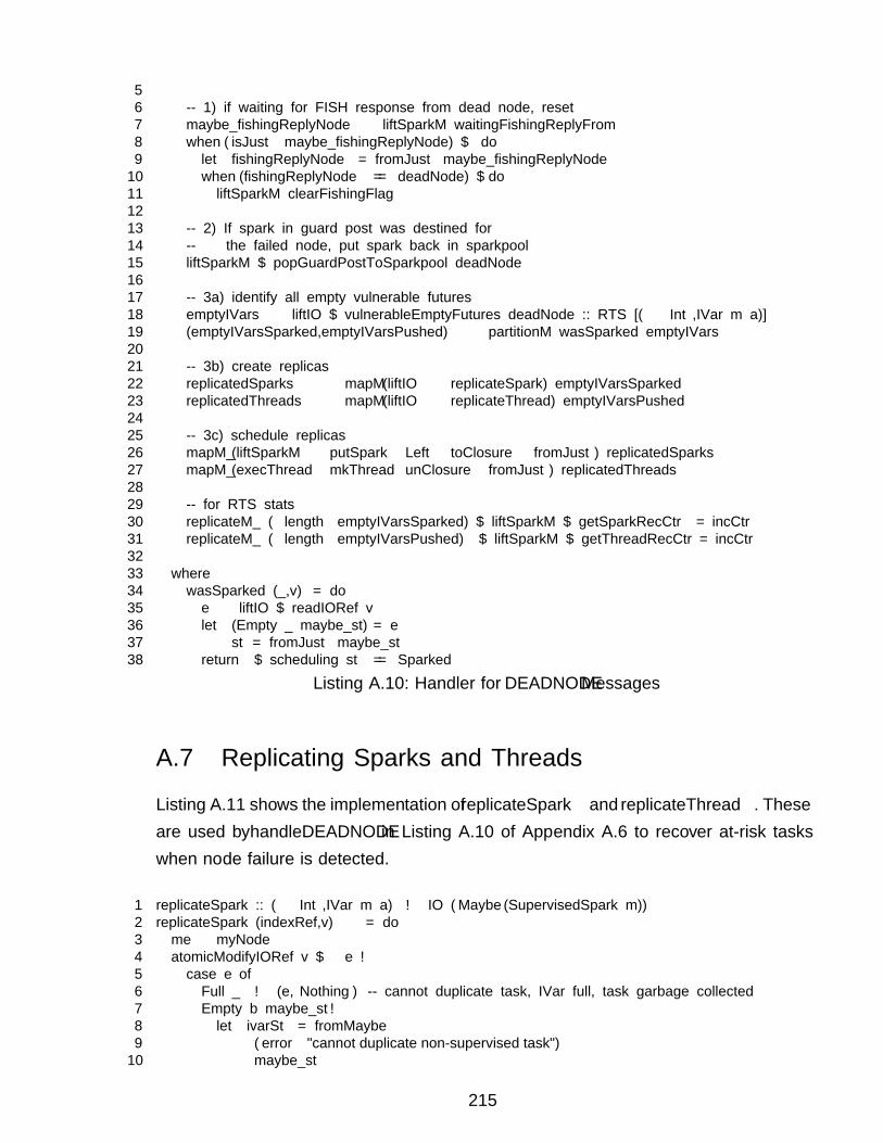
56 -- 1) if waiting for FISH response from dead node, reset7 maybe_fishingReplyNode ← liftSparkM waitingFishingReplyFrom8 when (isJust maybe_fishingReplyNode) $ do9 let fishingReplyNode = fromJust maybe_fishingReplyNode10 when (fishingReplyNode == deadNode) $ do11 liftSparkM clearFishingFlag1213 -- 2) If spark in guard post was destined for14 -- the failed node, put spark back in sparkpool15 liftSparkM $ popGuardPostToSparkpool deadNode1617 -- 3a) identify all empty vulnerable futures18 emptyIVars ← liftIO $ vulnerableEmptyFutures deadNode :: RTS [(Int,IVar m a)]19 (emptyIVarsSparked,emptyIVarsPushed) ← partitionM wasSparked emptyIVars2021 -- 3b) create replicas22 replicatedSparks ← mapM (liftIO ◦ replicateSpark) emptyIVarsSparked23 replicatedThreads ← mapM (liftIO ◦ replicateThread) emptyIVarsPushed2425 -- 3c) schedule replicas26 mapM_ (liftSparkM ◦ putSpark ◦ Left ◦ toClosure ◦ fromJust) replicatedSparks27 mapM_ (execThread ◦ mkThread ◦ unClosure ◦ fromJust) replicatedThreads2829 -- for RTS stats30 replicateM_ (length emptyIVarsSparked) $ liftSparkM $ getSparkRecCtr »= incCtr31 replicateM_ (length emptyIVarsPushed) $ liftSparkM $ getThreadRecCtr »= incCtr3233 where34 wasSparked (_,v) = do35 e ← liftIO $ readIORef v36 let (Empty _ maybe_st) = e37 st = fromJust maybe_st38 return $ scheduling st == Sparked

Listing A.10: Handler for DEADNODE Messages

A.7 Replicating Sparks and Threads

Listing A.11 shows the implementation of replicateSpark and replicateThread. Theseare used by handleDEADNODE in Listing A.10 of Appendix A.6 to recover at-risk taskswhen node failure is detected.

1 replicateSpark :: (Int,IVar m a) → IO (Maybe (SupervisedSpark m))2 replicateSpark (indexRef,v) = do3 me ← myNode4 atomicModifyIORef v $ λe →5 case e of6 Full _ → (e,Nothing) -- cannot duplicate task, IVar full, task garbage collected7 Empty b maybe_st →8 let ivarSt = fromMaybe9 (error "cannot␣duplicate␣non-supervised␣task")10 maybe_st

215

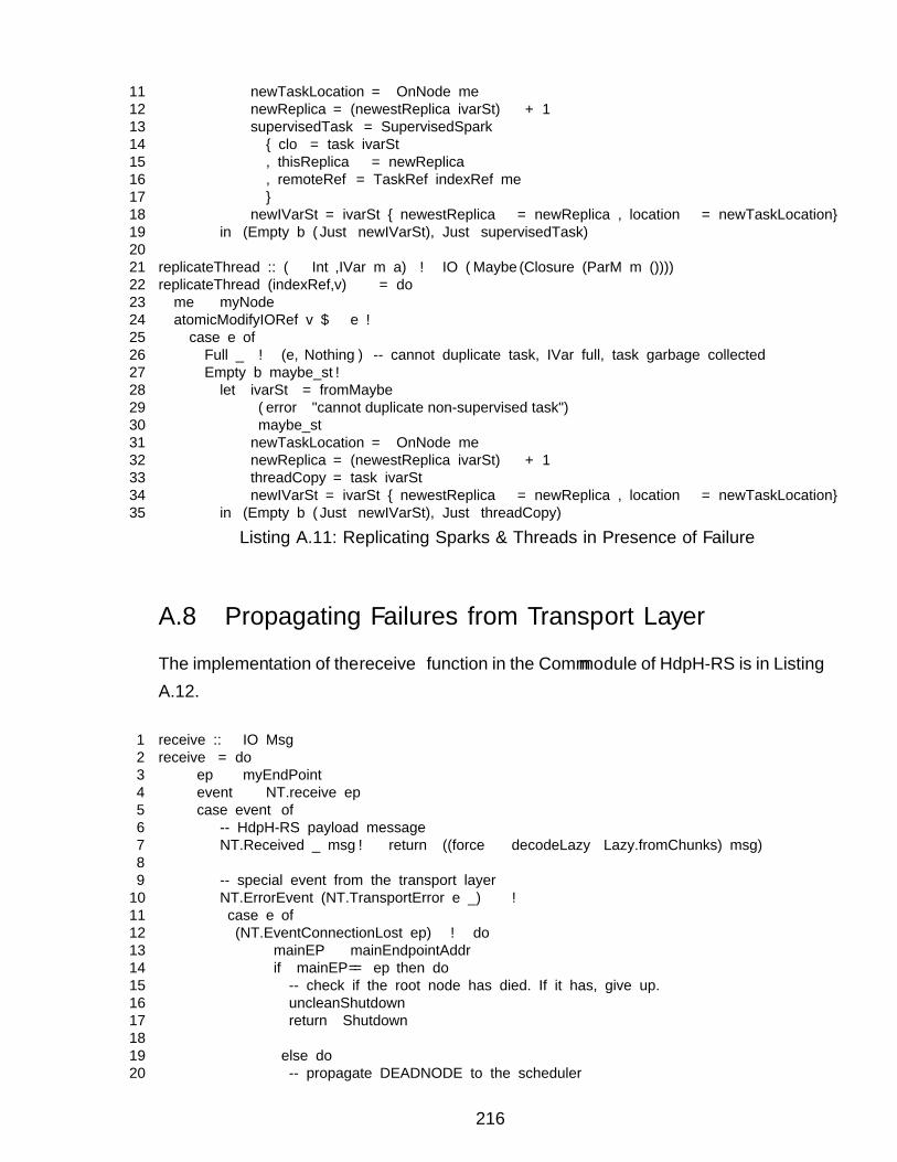
11 newTaskLocation = OnNode me12 newReplica = (newestReplica ivarSt) + 113 supervisedTask = SupervisedSpark14 { clo = task ivarSt15 , thisReplica = newReplica16 , remoteRef = TaskRef indexRef me17 }18 newIVarSt = ivarSt { newestReplica = newReplica , location = newTaskLocation}19 in (Empty b (Just newIVarSt),Just supervisedTask)2021 replicateThread :: (Int,IVar m a) → IO (Maybe (Closure (ParM m ())))22 replicateThread (indexRef,v) = do23 me ← myNode24 atomicModifyIORef v $ λe →25 case e of26 Full _ → (e,Nothing) -- cannot duplicate task, IVar full, task garbage collected27 Empty b maybe_st →28 let ivarSt = fromMaybe29 (error "cannot␣duplicate␣non-supervised␣task")30 maybe_st31 newTaskLocation = OnNode me32 newReplica = (newestReplica ivarSt) + 133 threadCopy = task ivarSt34 newIVarSt = ivarSt { newestReplica = newReplica , location = newTaskLocation}35 in (Empty b (Just newIVarSt),Just threadCopy)

Listing A.11: Replicating Sparks & Threads in Presence of Failure

A.8 Propagating Failures from Transport Layer

The implementation of the receive function in the Commmodule of HdpH-RS is in ListingA.12.

1 receive :: IO Msg2 receive = do3 ep ← myEndPoint4 event ← NT.receive ep5 case event of6 -- HdpH-RS payload message7 NT.Received _ msg → return ((force ◦ decodeLazy ◦ Lazy.fromChunks) msg)89 -- special event from the transport layer10 NT.ErrorEvent (NT.TransportError e _) →11 case e of12 (NT.EventConnectionLost ep) → do13 mainEP ← mainEndpointAddr14 if mainEP == ep then do15 -- check if the root node has died. If it has, give up.16 uncleanShutdown17 return Shutdown1819 else do20 -- propagate DEADNODE to the scheduler

216

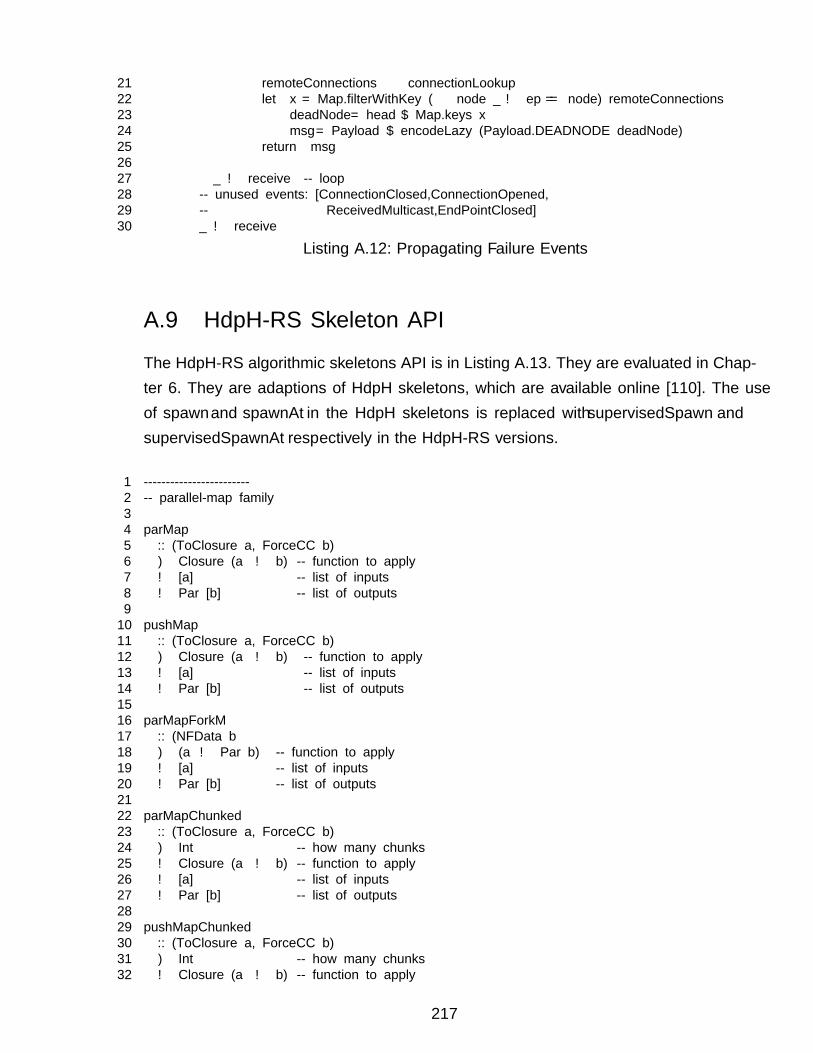
21 remoteConnections ← connectionLookup22 let x = Map.filterWithKey (λnode _ → ep == node) remoteConnections23 deadNode = head $ Map.keys x24 msg = Payload $ encodeLazy (Payload.DEADNODE deadNode)25 return msg2627 _ → receive -- loop28 -- unused events: [ConnectionClosed,ConnectionOpened,29 -- ReceivedMulticast,EndPointClosed]30 _ → receive

Listing A.12: Propagating Failure Events

A.9 HdpH-RS Skeleton API

The HdpH-RS algorithmic skeletons API is in Listing A.13. They are evaluated in Chap-ter 6. They are adaptions of HdpH skeletons, which are available online [110]. The useof spawn and spawnAt in the HdpH skeletons is replaced with supervisedSpawn andsupervisedSpawnAt respectively in the HdpH-RS versions.

1 ------------------------2 -- parallel-map family34 parMap5 :: (ToClosure a, ForceCC b)6 ⇒ Closure (a → b) -- function to apply7 → [a] -- list of inputs8 → Par [b] -- list of outputs910 pushMap11 :: (ToClosure a, ForceCC b)12 ⇒ Closure (a → b) -- function to apply13 → [a] -- list of inputs14 → Par [b] -- list of outputs1516 parMapForkM17 :: (NFData b18 ⇒ (a → Par b) -- function to apply19 → [a] -- list of inputs20 → Par [b] -- list of outputs2122 parMapChunked23 :: (ToClosure a, ForceCC b)24 ⇒ Int -- how many chunks25 → Closure (a → b) -- function to apply26 → [a] -- list of inputs27 → Par [b] -- list of outputs2829 pushMapChunked30 :: (ToClosure a, ForceCC b)31 ⇒ Int -- how many chunks32 → Closure (a → b) -- function to apply

217

33 → [a] -- list of inputs34 → Par [b] -- list of outputs3536 parMapSliced37 :: (ToClosure a, ForceCC b)38 ⇒ Int -- how many slices39 → Closure (a → b) -- function to apply40 → [a] -- list of inputs41 → Par [b] -- list of outputs4243 pushMapSliced44 :: (ToClosure a, ForceCC b)45 ⇒ Int -- how many slices46 → Closure (a → b) -- function to apply47 → [a] -- list of inputs48 → Par [b] -- list of outputs4950 ------------------------51 -- divide-and-conquer family5253 forkDivideAndConquer54 :: (NFData b)55 ⇒ (a → Bool) -- isTrivial56 → (a → [a]) -- decompose problem57 → (a → [b] → b) -- combine solutions58 → (a → Par b) -- trivial algorithm59 → a -- problem60 → Par b -- result6162 parDivideAndConquer63 :: Closure (Closure a → Bool) -- is trivial64 → Closure (Closure a → [Closure a]) -- decompose problem65 → Closure (Closure a → [Closure b] → Closure b) -- combine solutions66 → Closure (Closure a → Par (Closure b)) --trivial algorithm67 → Closure a -- problem68 → Par (Closure b) -- result6970 pushDivideAndConquer71 :: Closure (Closure a → Bool) -- is trivial72 → Closure (Closure a → [Closure a]) -- decompose problem73 → Closure (Closure a → [Closure b] → Closure b) -- combine solutions74 → Closure (Closure a → Par (Closure b)) -- trivial algorithm75 → Closure a -- problem76 → Par (Closure b) -- result7778 ------------------------79 -- map-reduce family8081 parMapReduceRangeThresh82 :: Closure Int -- threshold83 → Closure InclusiveRange -- range over which to calculate84 → Closure (Closure Int → Par (Closure a)) -- compute one result85 → Closure (Closure a → Closure a → Par (Closure a)) -- compute two results (associate)86 → Closure a -- initial value87 → Par (Closure a)8889 pushMapReduceRangeThresh

218

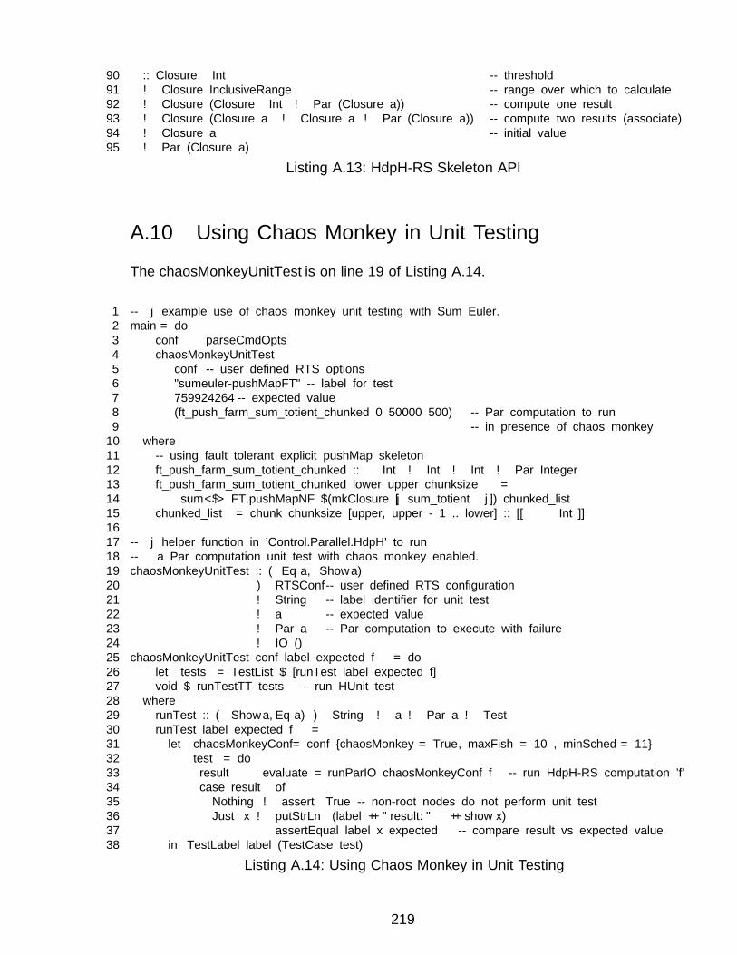
90 :: Closure Int -- threshold91 → Closure InclusiveRange -- range over which to calculate92 → Closure (Closure Int → Par (Closure a)) -- compute one result93 → Closure (Closure a → Closure a → Par (Closure a)) -- compute two results (associate)94 → Closure a -- initial value95 → Par (Closure a)

Listing A.13: HdpH-RS Skeleton API

A.10 Using Chaos Monkey in Unit Testing

The chaosMonkeyUnitTest is on line 19 of Listing A.14.

1 -- | example use of chaos monkey unit testing with Sum Euler.2 main = do3 conf ← parseCmdOpts4 chaosMonkeyUnitTest5 conf -- user defined RTS options6 "sumeuler-pushMapFT" -- label for test7 759924264 -- expected value8 (ft_push_farm_sum_totient_chunked 0 50000 500) -- Par computation to run9 -- in presence of chaos monkey10 where11 -- using fault tolerant explicit pushMap skeleton12 ft_push_farm_sum_totient_chunked :: Int → Int → Int → Par Integer13 ft_push_farm_sum_totient_chunked lower upper chunksize =14 sum <$> FT.pushMapNF $(mkClosure [ | sum_totient |]) chunked_list15 chunked_list = chunk chunksize [upper, upper - 1 .. lower] :: [[Int]]1617 -- | helper function in ’Control.Parallel.HdpH’ to run18 -- a Par computation unit test with chaos monkey enabled.19 chaosMonkeyUnitTest :: (Eq a, Show a)20 ⇒ RTSConf -- user defined RTS configuration21 → String -- label identifier for unit test22 → a -- expected value23 → Par a -- Par computation to execute with failure24 → IO ()25 chaosMonkeyUnitTest conf label expected f = do26 let tests = TestList $ [runTest label expected f]27 void $ runTestTT tests -- run HUnit test28 where29 runTest :: (Show a,Eq a) ⇒ String → a → Par a → Test30 runTest label expected f =31 let chaosMonkeyConf = conf {chaosMonkey = True, maxFish = 10 , minSched = 11}32 test = do33 result ← evaluate =« runParIO chaosMonkeyConf f -- run HdpH-RS computation ’f’34 case result of35 Nothing → assert True -- non-root nodes do not perform unit test36 Just x → putStrLn (label++"␣result:␣"++show x) »37 assertEqual label x expected -- compare result vs expected value38 in TestLabel label (TestCase test)

Listing A.14: Using Chaos Monkey in Unit Testing

219

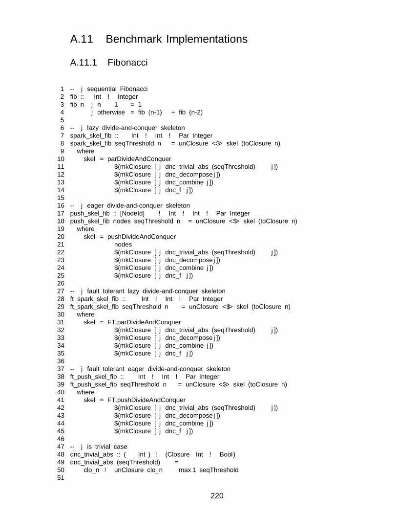
A.11 Benchmark Implementations

A.11.1 Fibonacci

1 -- | sequential Fibonacci2 fib :: Int → Integer3 fib n | n ≤ 1 = 14 | otherwise = fib (n-1) + fib (n-2)56 -- | lazy divide-and-conquer skeleton7 spark_skel_fib :: Int → Int → Par Integer8 spark_skel_fib seqThreshold n = unClosure <$> skel (toClosure n)9 where10 skel = parDivideAndConquer11 $(mkClosure [ | dnc_trivial_abs (seqThreshold) |])12 $(mkClosure [ | dnc_decompose |])13 $(mkClosure [ | dnc_combine |])14 $(mkClosure [ | dnc_f |])1516 -- | eager divide-and-conquer skeleton17 push_skel_fib :: [NodeId] → Int → Int → Par Integer18 push_skel_fib nodes seqThreshold n = unClosure <$> skel (toClosure n)19 where20 skel = pushDivideAndConquer21 nodes22 $(mkClosure [ | dnc_trivial_abs (seqThreshold) |])23 $(mkClosure [ | dnc_decompose |])24 $(mkClosure [ | dnc_combine |])25 $(mkClosure [ | dnc_f |])2627 -- | fault tolerant lazy divide-and-conquer skeleton28 ft_spark_skel_fib :: Int → Int → Par Integer29 ft_spark_skel_fib seqThreshold n = unClosure <$> skel (toClosure n)30 where31 skel = FT.parDivideAndConquer32 $(mkClosure [ | dnc_trivial_abs (seqThreshold) |])33 $(mkClosure [ | dnc_decompose |])34 $(mkClosure [ | dnc_combine |])35 $(mkClosure [ | dnc_f |])3637 -- | fault tolerant eager divide-and-conquer skeleton38 ft_push_skel_fib :: Int → Int → Par Integer39 ft_push_skel_fib seqThreshold n = unClosure <$> skel (toClosure n)40 where41 skel = FT.pushDivideAndConquer42 $(mkClosure [ | dnc_trivial_abs (seqThreshold) |])43 $(mkClosure [ | dnc_decompose |])44 $(mkClosure [ | dnc_combine |])45 $(mkClosure [ | dnc_f |])4647 -- | is trivial case48 dnc_trivial_abs :: (Int) → (Closure Int → Bool)49 dnc_trivial_abs (seqThreshold) =50 λ clo_n → unClosure clo_n ≤ max 1 seqThreshold51

220

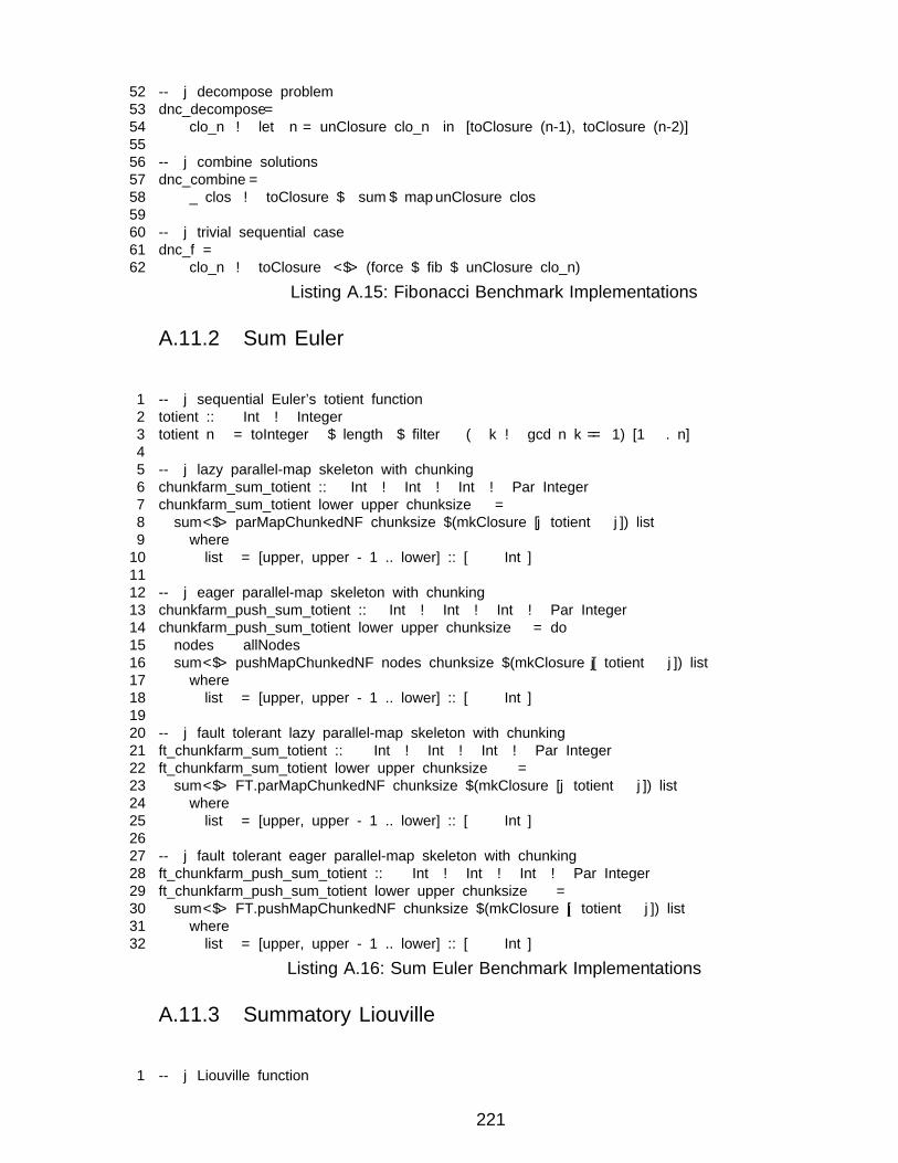
52 -- | decompose problem53 dnc_decompose =54 λ clo_n → let n = unClosure clo_n in [toClosure (n-1), toClosure (n-2)]5556 -- | combine solutions57 dnc_combine =58 λ _ clos → toClosure $ sum $ map unClosure clos5960 -- | trivial sequential case61 dnc_f =62 λ clo_n → toClosure <$> (force $ fib $ unClosure clo_n)

Listing A.15: Fibonacci Benchmark Implementations

A.11.2 Sum Euler

1 -- | sequential Euler’s totient function2 totient :: Int → Integer3 totient n = toInteger $ length $ filter (λ k → gcd n k == 1) [1 ◦ . n]45 -- | lazy parallel-map skeleton with chunking6 chunkfarm_sum_totient :: Int → Int → Int → Par Integer7 chunkfarm_sum_totient lower upper chunksize =8 sum <$> parMapChunkedNF chunksize $(mkClosure [ | totient |]) list9 where10 list = [upper, upper - 1 .. lower] :: [Int]1112 -- | eager parallel-map skeleton with chunking13 chunkfarm_push_sum_totient :: Int → Int → Int → Par Integer14 chunkfarm_push_sum_totient lower upper chunksize = do15 nodes ← allNodes16 sum <$> pushMapChunkedNF nodes chunksize $(mkClosure [ | totient |]) list17 where18 list = [upper, upper - 1 .. lower] :: [Int]1920 -- | fault tolerant lazy parallel-map skeleton with chunking21 ft_chunkfarm_sum_totient :: Int → Int → Int → Par Integer22 ft_chunkfarm_sum_totient lower upper chunksize =23 sum <$> FT.parMapChunkedNF chunksize $(mkClosure [ | totient |]) list24 where25 list = [upper, upper - 1 .. lower] :: [Int]2627 -- | fault tolerant eager parallel-map skeleton with chunking28 ft_chunkfarm_push_sum_totient :: Int → Int → Int → Par Integer29 ft_chunkfarm_push_sum_totient lower upper chunksize =30 sum <$> FT.pushMapChunkedNF chunksize $(mkClosure [ | totient |]) list31 where32 list = [upper, upper - 1 .. lower] :: [Int]

Listing A.16: Sum Euler Benchmark Implementations

A.11.3 Summatory Liouville

1 -- | Liouville function

221

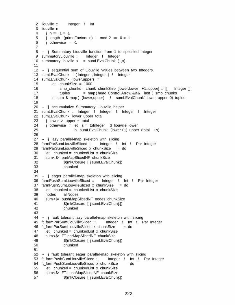
2 liouville :: Integer → Int3 liouville n4 | n == 1 = 15 | length (primeFactors n) ‘mod‘ 2 == 0 = 16 | otherwise = -178 -- | Summatory Liouville function from 1 to specified Integer9 summatoryLiouville :: Integer → Integer10 summatoryLiouville x = sumLEvalChunk (1,x)1112 -- | sequential sum of Liouville values between two Integers.13 sumLEvalChunk :: (Integer,Integer) → Integer14 sumLEvalChunk (lower,upper) =15 let chunkSize = 100016 smp_chunks = chunk chunkSize [lower,lower+1..upper] :: [[Integer]]17 tuples = map (head Control.Arrow.&&& last) smp_chunks18 in sum $ map (λ(lower,upper) → sumLEvalChunk’ lower upper 0) tuples1920 -- | accumulative Summatory Liouville helper21 sumLEvalChunk’ :: Integer → Integer → Integer → Integer22 sumLEvalChunk’ lower upper total23 | lower > upper = total24 | otherwise = let s = toInteger $ liouville lower25 in sumLEvalChunk’ (lower+1) upper (total+s)2627 -- | lazy parallel-map skeleton with slicing28 farmParSumLiouvilleSliced :: Integer → Int → Par Integer29 farmParSumLiouvilleSliced x chunkSize = do30 let chunked = chunkedList x chunkSize31 sum <$> parMapSlicedNF chunkSize32 $(mkClosure [ |sumLEvalChunk |])33 chunked3435 -- | eager parallel-map skeleton with slicing36 farmPushSumLiouvilleSliced :: Integer → Int → Par Integer37 farmPushSumLiouvilleSliced x chunkSize = do38 let chunked = chunkedList x chunkSize39 nodes ← allNodes40 sum <$> pushMapSlicedNF nodes chunkSize41 $(mkClosure [ |sumLEvalChunk |])42 chunked4344 -- | fault tolerant lazy parallel-map skeleton with slicing45 ft_farmParSumLiouvilleSliced :: Integer → Int → Par Integer46 ft_farmParSumLiouvilleSliced x chunkSize = do47 let chunked = chunkedList x chunkSize48 sum <$> FT.parMapSlicedNF chunkSize49 $(mkClosure [ |sumLEvalChunk |])50 chunked5152 -- | fault tolerant eager parallel-map skeleton with slicing53 ft_farmPushSumLiouvilleSliced :: Integer → Int → Par Integer54 ft_farmPushSumLiouvilleSliced x chunkSize = do55 let chunked = chunkedList x chunkSize56 sum <$> FT.pushMapSlicedNF chunkSize57 $(mkClosure [ |sumLEvalChunk |])

222

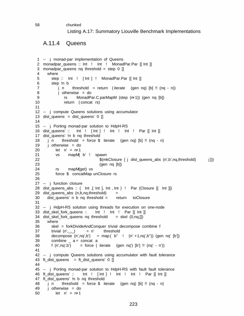
58 chunked

Listing A.17: Summatory Liouville Benchmark Implementations

A.11.4 Queens

1 -- | monad-par implementation of Queens2 monadpar_queens :: Int → Int → MonadPar.Par [[Int]]3 monadpar_queens nq threshold = step 0 []4 where5 step :: Int → [Int] → MonadPar.Par [[Int]]6 step !n b7 | n ≥ threshold = return (iterate (gen nq) [b] !! (nq - n))8 | otherwise = do9 rs ← MonadPar.C.parMapM (step (n+1)) (gen nq [b])10 return (concat rs)1112 -- | compute Queens solutions using accumulator13 dist_queens = dist_queens’ 0 []1415 -- | Porting monad-par solution to HdpH-RS16 dist_queens’ :: Int → [Int] → Int → Int → Par [[Int]]17 dist_queens’ !n b nq threshold18 | n ≥ threshold = force $ iterate (gen nq) [b] !! (nq - n)19 | otherwise = do20 let n’ = n+121 vs ← mapM (λb’ → spawn22 $(mkClosure [ | dist_queens_abs (n’,b’,nq,threshold) |]))23 (gen nq [b])24 rs ← mapM (get) vs25 force $ concatMap unClosure rs2627 -- | function closure28 dist_queens_abs :: (Int,[Int],Int,Int) → Par (Closure [[Int]])29 dist_queens_abs (n,b,nq,threshold) =30 dist_queens’ n b nq threshold »= return ◦ toClosure3132 -- | HdpH-RS solution using threads for execution on one-node33 dist_skel_fork_queens :: Int → Int → Par [[Int]]34 dist_skel_fork_queens nq threshold = skel (0,nq,[])35 where36 skel = forkDivideAndConquer trivial decompose combine f37 trivial (n’,_,_) = n’ ≥ threshold38 decompose (n’,nq’,b’) = map (λb’’ → (n’+1,nq’,b’’)) (gen nq’ [b’])39 combine _ a = concat a40 f (n’,nq’,b’) = force (iterate (gen nq’) [b’] !! (nq’ - n’))4142 -- | compute Queens solutions using accumulator with fault tolerance43 ft_dist_queens = ft_dist_queens’ 0 []4445 -- | Porting monad-par solution to HdpH-RS with fault fault tolerance46 ft_dist_queens’ :: Int → [Int] → Int → Int → Par [[Int]]47 ft_dist_queens’ !n b nq threshold48 | n ≥ threshold = force $ iterate (gen nq) [b] !! (nq - n)49 | otherwise = do50 let n’ = n+1

223

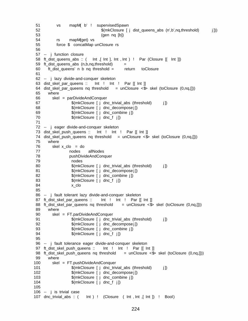
51 vs ← mapM (λb’ → supervisedSpawn52 $(mkClosure [ | dist_queens_abs (n’,b’,nq,threshold) |]))53 (gen nq [b])54 rs ← mapM (get) vs55 force $ concatMap unClosure rs5657 -- | function closure58 ft_dist_queens_abs :: (Int,[Int],Int,Int) → Par (Closure [[Int]])59 ft_dist_queens_abs (n,b,nq,threshold) =60 ft_dist_queens’ n b nq threshold »= return ◦ toClosure6162 -- | lazy divide-and-conquer skeleton63 dist_skel_par_queens :: Int → Int → Par [[Int]]64 dist_skel_par_queens nq threshold = unClosure <$> skel (toClosure (0,nq,[]))65 where66 skel = parDivideAndConquer67 $(mkClosure [ | dnc_trivial_abs (threshold) |])68 $(mkClosure [ | dnc_decompose |])69 $(mkClosure [ | dnc_combine |])70 $(mkClosure [ | dnc_f |])7172 -- | eager divide-and-conquer skeleton73 dist_skel_push_queens :: Int → Int → Par [[Int]]74 dist_skel_push_queens nq threshold = unClosure <$> skel (toClosure (0,nq,[]))75 where76 skel x_clo = do77 nodes ← allNodes78 pushDivideAndConquer79 nodes80 $(mkClosure [ | dnc_trivial_abs (threshold) |])81 $(mkClosure [ | dnc_decompose |])82 $(mkClosure [ | dnc_combine |])83 $(mkClosure [ | dnc_f |])84 x_clo8586 -- | fault tolerant lazy divide-and-conquer skeleton87 ft_dist_skel_par_queens :: Int → Int → Par [[Int]]88 ft_dist_skel_par_queens nq threshold = unClosure <$> skel (toClosure (0,nq,[]))89 where90 skel = FT.parDivideAndConquer91 $(mkClosure [ | dnc_trivial_abs (threshold) |])92 $(mkClosure [ | dnc_decompose |])93 $(mkClosure [ | dnc_combine |])94 $(mkClosure [ | dnc_f |])9596 -- | fault tolerance eager divide-and-conquer skeleton97 ft_dist_skel_push_queens :: Int → Int → Par [[Int]]98 ft_dist_skel_push_queens nq threshold = unClosure <$> skel (toClosure (0,nq,[]))99 where100 skel = FT.pushDivideAndConquer101 $(mkClosure [ | dnc_trivial_abs (threshold) |])102 $(mkClosure [ | dnc_decompose |])103 $(mkClosure [ | dnc_combine |])104 $(mkClosure [ | dnc_f |])105106 -- | is trivial case107 dnc_trivial_abs :: (Int) → (Closure (Int,Int,[Int]) → Bool)

224

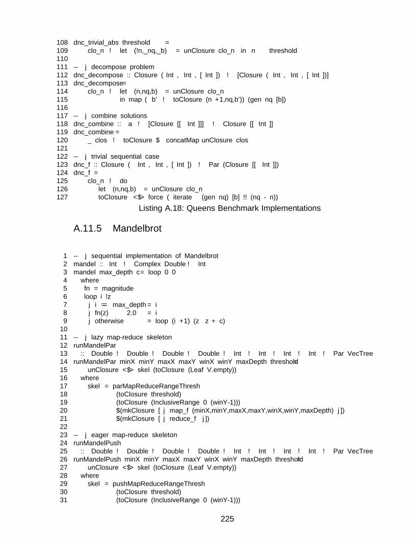
108 dnc_trivial_abs threshold =109 λ clo_n → let (!n,_nq,_b) = unClosure clo_n in n ≥ threshold110111 -- | decompose problem112 dnc_decompose :: Closure (Int, Int, [Int]) → [Closure (Int, Int, [Int])]113 dnc_decompose =114 λ clo_n → let (n,nq,b) = unClosure clo_n115 in map (λb’ → toClosure (n+1,nq,b’)) (gen nq [b])116117 -- | combine solutions118 dnc_combine :: a → [Closure [[Int]]] → Closure [[Int]]119 dnc_combine =120 λ _ clos → toClosure $ concatMap unClosure clos121122 -- | trivial sequential case123 dnc_f :: Closure (Int, Int, [Int]) → Par (Closure [[Int]])124 dnc_f =125 λ clo_n → do126 let (n,nq,b) = unClosure clo_n127 toClosure <$> force (iterate (gen nq) [b] !! (nq - n))

Listing A.18: Queens Benchmark Implementations

A.11.5 Mandelbrot

1 -- | sequential implementation of Mandelbrot2 mandel :: Int → Complex Double → Int3 mandel max_depth c = loop 0 04 where5 fn = magnitude6 loop i !z7 | i == max_depth = i8 | fn(z) ≥ 2.0 = i9 | otherwise = loop (i+1) (z∗z + c)1011 -- | lazy map-reduce skeleton12 runMandelPar13 :: Double → Double → Double → Double → Int → Int → Int → Int → Par VecTree14 runMandelPar minX minY maxX maxY winX winY maxDepth threshold =15 unClosure <$> skel (toClosure (Leaf V.empty))16 where17 skel = parMapReduceRangeThresh18 (toClosure threshold)19 (toClosure (InclusiveRange 0 (winY-1)))20 $(mkClosure [ | map_f (minX,minY,maxX,maxY,winX,winY,maxDepth) |])21 $(mkClosure [ | reduce_f |])2223 -- | eager map-reduce skeleton24 runMandelPush25 :: Double → Double → Double → Double → Int → Int → Int → Int → Par VecTree26 runMandelPush minX minY maxX maxY winX winY maxDepth threshold =27 unClosure <$> skel (toClosure (Leaf V.empty))28 where29 skel = pushMapReduceRangeThresh30 (toClosure threshold)31 (toClosure (InclusiveRange 0 (winY-1)))

225

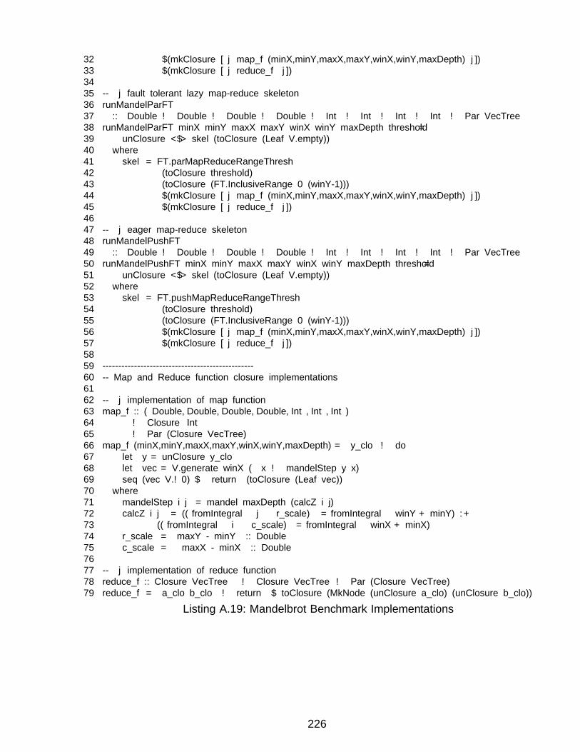
32 $(mkClosure [ | map_f (minX,minY,maxX,maxY,winX,winY,maxDepth) |])33 $(mkClosure [ | reduce_f |])3435 -- | fault tolerant lazy map-reduce skeleton36 runMandelParFT37 :: Double → Double → Double → Double → Int → Int → Int → Int → Par VecTree38 runMandelParFT minX minY maxX maxY winX winY maxDepth threshold =39 unClosure <$> skel (toClosure (Leaf V.empty))40 where41 skel = FT.parMapReduceRangeThresh42 (toClosure threshold)43 (toClosure (FT.InclusiveRange 0 (winY-1)))44 $(mkClosure [ | map_f (minX,minY,maxX,maxY,winX,winY,maxDepth) |])45 $(mkClosure [ | reduce_f |])4647 -- | eager map-reduce skeleton48 runMandelPushFT49 :: Double → Double → Double → Double → Int → Int → Int → Int → Par VecTree50 runMandelPushFT minX minY maxX maxY winX winY maxDepth threshold =51 unClosure <$> skel (toClosure (Leaf V.empty))52 where53 skel = FT.pushMapReduceRangeThresh54 (toClosure threshold)55 (toClosure (FT.InclusiveRange 0 (winY-1)))56 $(mkClosure [ | map_f (minX,minY,maxX,maxY,winX,winY,maxDepth) |])57 $(mkClosure [ | reduce_f |])5859 ------------------------------------------------60 -- Map and Reduce function closure implementations6162 -- | implementation of map function63 map_f :: (Double,Double,Double,Double,Int,Int,Int)64 → Closure Int65 → Par (Closure VecTree)66 map_f (minX,minY,maxX,maxY,winX,winY,maxDepth) = λy_clo → do67 let y = unClosure y_clo68 let vec = V.generate winX (λx → mandelStep y x)69 seq (vec V.! 0) $ return (toClosure (Leaf vec))70 where71 mandelStep i j = mandel maxDepth (calcZ i j)72 calcZ i j = ((fromIntegral j ∗ r_scale) / fromIntegral winY + minY) :+73 ((fromIntegral i ∗ c_scale) / fromIntegral winX + minX)74 r_scale = maxY - minY :: Double75 c_scale = maxX - minX :: Double7677 -- | implementation of reduce function78 reduce_f :: Closure VecTree → Closure VecTree → Par (Closure VecTree)79 reduce_f = λa_clo b_clo → return $ toClosure (MkNode (unClosure a_clo) (unClosure b_clo))

Listing A.19: Mandelbrot Benchmark Implementations

226