RELIABILITY BASED SAFETY ASSESSMENT OF BURIED …etd.lib.metu.edu.tr/upload/12615423/index.pdf ·...

RELIABILITY BASED SAFETY ASSESSMENT OF BURIED CONTINUOUS PIPELINES SUBJECTED TO EARTHQUAKE EFFECTS

A THESIS SUBMITTED TO

THE GRADUATE SCHOOL OF NATURAL AND APPLIED SCIENCES OF

MIDDLE EAST TECHNICAL UNIVERSITY

BY

ERCAN AYKAN YAVUZ

IN PARTIAL FULFILLMENT OF THE REQUIREMENTS FOR

THE DEGREE OF MASTER OF SCIENCE IN

CIVIL ENGINEERING

JANUARY 2013

Approval of the thesis:


submitted by ERCAN AYKAN YAVUZ in partial fulfillment of the requirements for the degree of Master of Science in Civil Engineering Department, Middle East Technical University by, Prof. Dr. Canan Özgen Dean, Graduate School of Natural and Applied Sciences _____________________ Prof. Dr. Ahmet Cevdet Yalçıner Head of Department, Civil Engineering _____________________ Prof. Dr. M. Semih Yücemen Supervisor, Civil Engineering Dept., METU _____________________ Examining Committee Members: Prof. Dr. Sadık Bakır Civil Engineering Dept., METU _____________________ Prof. Dr. M. Semih Yücemen Civil Engineering Dept., METU _____________________ Assoc. Prof. Dr. Ayşegül Askan Gündoğan Civil Engineering Dept., METU _____________________ Assoc. Prof. Dr. Alp Caner Civil Engineering Dept., METU _____________________ Dr. Nazan Kılıç Disaster and Emergency Management Presidency _____________________ Date: _____________________

iv

I hereby declare that all information in this document has been obtained and presented in accordance with academic rules and ethical conduct. I also declare that, as required by these rules and conduct, I have fully cited and referenced all material and results that are not original to this work. Name, Last name : Ercan Aykan YAVUZ Signature :

v

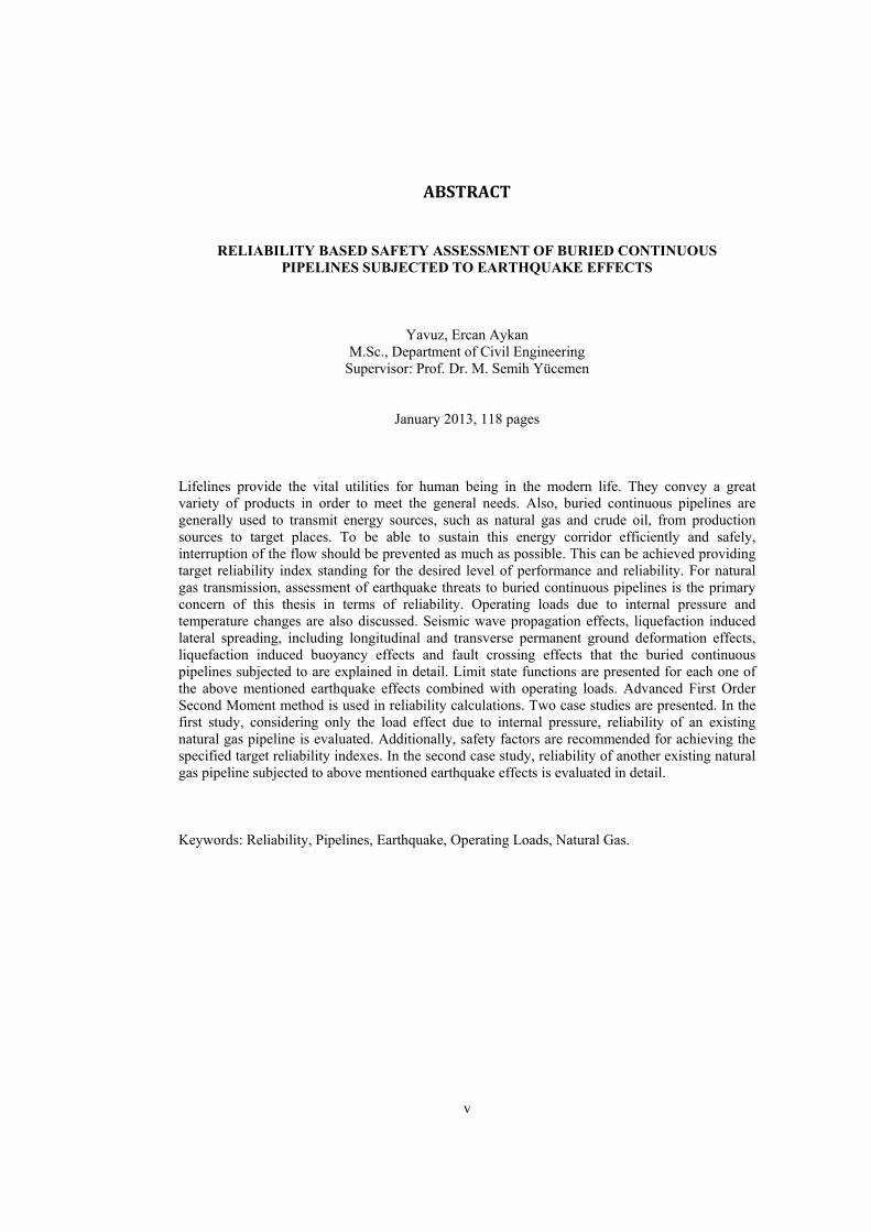
ABSTRACT


Yavuz, Ercan Aykan M.Sc., Department of Civil Engineering

Supervisor: Prof. Dr. M. Semih Yücemen

January 2013, 118 pages

Lifelines provide the vital utilities for human being in the modern life. They convey a great variety of products in order to meet the general needs. Also, buried continuous pipelines are generally used to transmit energy sources, such as natural gas and crude oil, from production sources to target places. To be able to sustain this energy corridor efficiently and safely, interruption of the flow should be prevented as much as possible. This can be achieved providing target reliability index standing for the desired level of performance and reliability. For natural gas transmission, assessment of earthquake threats to buried continuous pipelines is the primary concern of this thesis in terms of reliability. Operating loads due to internal pressure and temperature changes are also discussed. Seismic wave propagation effects, liquefaction induced lateral spreading, including longitudinal and transverse permanent ground deformation effects, liquefaction induced buoyancy effects and fault crossing effects that the buried continuous pipelines subjected to are explained in detail. Limit state functions are presented for each one of the above mentioned earthquake effects combined with operating loads. Advanced First Order Second Moment method is used in reliability calculations. Two case studies are presented. In the first study, considering only the load effect due to internal pressure, reliability of an existing natural gas pipeline is evaluated. Additionally, safety factors are recommended for achieving the specified target reliability indexes. In the second case study, reliability of another existing natural gas pipeline subjected to above mentioned earthquake effects is evaluated in detail. Keywords: Reliability, Pipelines, Earthquake, Operating Loads, Natural Gas.

vi

ÖZ

DEPREM ETKİLERİNE MARUZ GÖMÜLÜ SÜREKLİ BORU HATLARININ EMNİYETLERİNİN GÜVENİRLİK ESASLI DEĞERLENDİRİLMESİ

Yavuz, Ercan Aykan Yüksek Lisans, İnşaat Mühendisliği Bölümü Tez Yöneticisi: Prof. Dr. M. Semih Yücemen

Ocak 2013, 118 sayfa

Can damarları şebekeleri insanlığa modern hayatta önemli faydalar sunmaktadır. Genel ihtiyaçlar nedeni ile çeşitli ürünleri taşımaktadırlar. Gömülü sürekli boru hatları da genellikle doğal gaz ve ham petrol gibi enerji kaynaklarını üretim yerlerinden hedeflenen yerlere iletmede kullanılmaktadır. Bu enerji koridorundaki akışı verimli ve güvenli bir şekilde sürdürebilmek için akışın kesilmesinin mümkün olduğunca önlenmesi gerekir. Arzu edilen güvenirlik düzeyine karşılık gelen hedef güvenirlik indeksinin sağlanmasıyla bu sonuca ulaşılabilir. Doğal gaz iletiminde, gömülü sürekli boru hatlarında deprem tehlikesinin güvenirlik açısından değerlendirilmesi, bu tezin temel ilgi alanını oluşturmaktadır. İç basınç ve sıcaklık değişimlerinden kaynaklanan işletme yüklerine de değinilmektedir. Gömülü sürekli boru hatlarının maruz kaldığı, sismik dalga hareketi etkileri, boyuna ve enine kalıcı yer değiştirme etkilerini içeren, sıvılaşma nedeniyle oluşan yanal yayılma etkileri, sıvılaşma nedeniyle oluşan kaldırma kuvveti etkileri ve fay geçişi etkileri detaylı bir şekilde açıklanmakta ve incelenmektedir. Bahsedilen her bir deprem etkisi için işletme yükleriyle birlikte limit durum fonksiyonları sunulmaktadır. Güvenirlik hesaplamalarında, Geliştirilmiş Birinci Mertebe İkinci Moment metodu kullanılmaktadır. İki adet örnek çalışma sunulmaktadır. İlk çalışmada, yük etkisi olarak sadece iç basınç düşünülerek mevcut bir doğal gaz boru hattının güvenirlik hesabı yapılmaktadır. Buna ilaveten hedef güvenirlik indeksleri için güvenlik katsayıları önerilmektedir. İkinci örnek çalışmada da yine bir mevcut doğal gaz boru hattı, söz konusu deprem etkileri altında güvenirlik açısından detaylı bir şekilde değerlendirilmektedir. Anahtar Kelimeler: Güvenilirlik, Boru Hatları, Deprem, İşletme Yükleri, Doğal Gaz.

vii

Benim için her türlü fedakarlığı gösteren Güzel Ailem’e

viii

ACKNOWLEDGMENTS The author wishes to express his deepest gratitude to his supervisor Prof. Dr. M. Semih Yücemen for his guidance, advice, criticism, encouragements and insight throughout the research. Although the duration of the thesis study was elongated, nevertheless the support of my supervisor did not decrease. The author, again, would like to thank his supervisor, Prof. Dr. M. Semih Yücemen. The author would also like to thank his wife Bilgehan Yavuz. Throughout the study of this thesis work, she has been always with the author and encouraged the author to complete the thesis. The author thanks his wife also for her help in preparing the maps presented in the thesis. And the author cannot go further without mentioning his dearie daughter, Zehra Ece Yavuz. She has to do nothing to help the author. Her presence was enough. And the author is grateful to his brothers, Mustafa Yavuz and Adnan Yavuz and his father, Ahmet Yavuz and his mother Azime Yavuz. They have always been beside the author with their encouragement and material support throughout the entire life of the author. Also the assistance of Ms. Filiz Armutlu, Mr. Mustafa Özdemir, Mr. Yasin Aslan, Mr. Ali Rıza Çırakoğlu and all friends are gratefully acknowledged.

ix

TABLEOFCONTENTS ABSTRACT.................................................................................................................................... v

ÖZ .................................................................................................................................................. vi

ACKNOWLEDGMENTS .......................................................................................................... viii

TABLE OF CONTENTS ............................................................................................................. ix

LIST OF TABLES ........................................................................................................................ xi

LIST OF FIGURES .................................................................................................................... xiv

LIST OF SYMBOLS AND ABBREVIATIONS ...................................................................... xvi

CHAPTERS

1. INTRODUCTION ................................................................................................................... 1

1.1 General View ........................................................................................................................ 1

1.2 Review of Related Work ....................................................................................................... 2

1.3 Aim and Scope of the Study .................................................................................................. 4

2. LOAD EFFECTS ON BURIED PIPELINES ........................................................................ 7

2.1 Introduction ........................................................................................................................... 7

2.2 Load due to Internal Pressure ................................................................................................ 8

2.3 Load due to Temperature Changes ........................................................................................ 9

2.3 Other Load Effects ................................................................................................................ 9

2.4 Strain Based Identification of Loads ..................................................................................... 9

3. EARTHQUAKE EFFECTS ON BURIED PIPELINES .................................................... 11

3.1 Introduction ......................................................................................................................... 11

3.2 Seismic Wave Propagation Effects ..................................................................................... 13

3.3 Permanent Ground Deformation Effects ............................................................................. 17

3.3.1 Liquefaction Induced Lateral Spreading ..................................................................... 18

3.3.1.1 Pipeline Subjected to Longitudinal PGD ............................................................. 21

3.3.1.2 Pipeline Subjected to Transverse PGD ................................................................ 26

3.3.2 Liquefaction Induced Buoyancy .................................................................................. 28

3.3.3 Fault Crossing ............................................................................................................. 32

3.3.3.1 Newmark Hall (1975) Method ............................................................................. 33

3.3.3.2 Kennedy et al. (1977) Method ............................................................................. 35

4. STRUCTURAL RELIABILITY ASSESSMENT OF BURIED PIPELINES .................. 39

4.1 Introduction ......................................................................................................................... 39

4.2 Structural Reliability Methods ............................................................................................ 39

4.2.1 The Classical Reliability Formulation ......................................................................... 39

x

4.2.2 First Order Second Moment Method ........................................................................... 40

4.2.2.1 Mean Value Method ............................................................................................ 42

4.2.2.2 Advanced First Order Second Moment Method .................................................. 43

4.3 Combination of Failure Modes ........................................................................................... 44

4.4 Uncertainty Modeling ......................................................................................................... 46

4.5 Identification and Description of Different Failure Modes ................................................. 47

4.5.1 Tensile Failure ............................................................................................................. 51

4.5.2 Local Buckling Failure ................................................................................................ 51

4.6 Determination of Limit State Functions .............................................................................. 52

4.7 Calculation of Survival Probability ..................................................................................... 54

5. CASE STUDIES..................................................................................................................... 55

5.1 Introduction ......................................................................................................................... 55

5.2 Case Study 1: Load due to Internal Pressure ....................................................................... 55

5.3 Case Study 2: Loads due to Internal Pressure, Temperature Changes and Earthquake Effects ....................................................................................................................................... 60

5.3.1 Load due to Seismic Wave Propagation Effects ......................................................... 61

5.3.2 Load due to Permanent Ground Deformation Effects ................................................. 78

5.3.2.1 Load due to Liquefaction Induced Lateral Spreading .......................................... 78

5.3.2.2 Load due to Liquefaction Induced Buoyancy ...................................................... 90

5.3.2.3 Load due to Fault Crossing .................................................................................. 91

5.3.3 Survival Probability of the Pipeline Subjected to Different Earthquake Effects ....... 100

6. SUMMARY AND CONCLUSIONS .................................................................................. 103

6.1 Summary ........................................................................................................................... 103

6.2 Conclusions ....................................................................................................................... 104

REFERENCES .......................................................................................................................... 107

APPENDICES

A. SOIL INDUCED FORCES ................................................................................................ 113

A.1 Axial Soil Force ............................................................................................................... 113

A.2 Lateral Soil Force ............................................................................................................. 114

B. SITE AND SOIL CLASSIFICATIONS ............................................................................ 117

xi

LISTOFTABLES

TABLES Table 2.1: Some of the Ramberg - Osgood parameters for steel pipes (Cited from O’Rourke et al., 1999) .............................................................................................................................................. 10 Table 3.1: Recommended values for length of PGD zone and for PGD (Cited from ALA, 2005) ....................................................................................................................................................... 20 Table 3.2: Recommended values for width of PGD zone and for PGD (Cited from ALA, 2005) 20 Table 4.1: Relationship between reliability index (β), probability of failure and expected performance level for normally distributed basic variables and linear failure functions (Cited from US Army Corps of Engineers, 1997) ............................................................................................. 41 Table 4.2: Mean values and coefficients of variation quantifying the aleatory uncertainties of basic variables ................................................................................................................................ 48 Table 4.3: Mean bias and epistemic uncertainties of basic variables ............................................ 50 Table 4.4: Tensile ( ) and compressive ( ) strain equations corresponding to each earthquake effect and the related method ......................................................................................................... 53 Table 5.1: Safety factors to be used in design (Cited from ASME B31.8, 2010) ......................... 56 Table 5.2: Nominal values of basic variables (Cited from BOTAŞ, 2009) ................................... 57 Table 5.3: Values of nominal wall thicknesses and internal radii as taken from BOTAŞ (2009) specifications and computed wall thicknesses for location classes for NPS 16 steel pipeline ....... 57 Table 5.4: Estimated values of the statistical parameters of the basic variables for the 16” Hatay Pipeline .......................................................................................................................................... 58 Table 5.5: Reliability indexes calculated based on different computer software corresponding to different location class and mean wall thickness combinations ..................................................... 59 Table 5.6: Target reliability indexes for different location classes for the Hatay pipeline as obtained from Equation 5.5 ........................................................................................................... 59 Table 5.7: Mean wall thickness values corresponding to target reliability indexes selected for different location classes ................................................................................................................ 60 Table 5.8: Existing safety factors and recommended safety factors corresponding to target reliabilities selected for different location classes considering the internal pressure as the only load effect ...................................................................................................................................... 60 Table 5.9: Nominal values of basic variables for Turkey-Greece Natural Gas Pipeline ............... 62 Table 5.10: Earthquakes with M ≥ 6.0 recorded in the Marmara region during the years 1905-1999 (Cited from Kalkan et al., 2009) ........................................................................................... 63 Table 5.11: Site coefficient, Fv, as a function of site class and PGVB (Cited from ALA, 2005 as modified from NEHRP, 1997) ....................................................................................................... 66 Table 5.12: Peak ground velocities at site class B and local design peak ground velocities at specified site classes corresponding to events having 10% and 2% probabilities of exceedance in 50 years, along the pipeline route .................................................................................................. 67 Table 5.13: Statistics of basic variables utilized in evaluating the seismic wave propagation effects ............................................................................................................................................. 69 Table 5.14: Computed mean of maximum frictional strain values which the pipeline may experience according to soil types ................................................................................................. 69 Table 5.15: Mean values of local design peak ground and seismic wave propagation velocities, axial strains and governing axial strains for events having 10% and 2% probabilities of exceedance in 50 years .................................................................................................................. 70 Table 5.16: Mean axial strain and the mean strain values for the segments where maximum frictional strain governs for events having 10% and 2% probabilities of exceedance in 50 years . 71

xii

Table 5.17: Means of highest and lowest maximum frictional strains for the segments having at least two major soil types, axial strain and marginal strain values for events having 10% and 2% probabilities of exceedance in 50 years ......................................................................................... 72 Table 5.18: Strain capacity, strain demands due to internal pressure, temperature changes, and case 1 (axial strain governs) of seismic wave propagation effects, corresponding reliability indexes and survival probabilities for local buckling failure mode for events having 10% and 2% probabilities of exceedance in 50 years ......................................................................................... 74 Table 5.19: Strain capacity, strain demands due to internal pressure, temperature changes, and case 2 (maximum frictional strain governs) of seismic wave propagation effects, corresponding reliability indexes and survival probabilities for local buckling failure mode for events having 10% and 2% probabilities of exceedance in 50 years .................................................................... 75 Table 5.20: Reliability indexes and survival probabilities of the pipeline experiencing marginal strains (marginal survival probabilities), survival probabilities corresponding to the average of the marginal survival probabilities for local buckling failure mode for events having 10% and 2% probabilities of exceedance in 50 years ......................................................................................... 75 Table 5.21: Reliability indexes and corresponding survival probabilities estimated for the different segments of the pipeline for the local buckling failure mode due to seismic wave propagation effects for events having 10% and 2% probabilities of exceedance in 50 years ........ 76 Table 5.22: Strain capacity, strain demands due to internal pressure, and temperature changes, highest tensile strain demands due to case 1 (axial strain governs) and case 2 (maximum frictional strain governs) of seismic wave propagation effects for events having 2% probabilities of exceedance in 50 years .................................................................................................................. 78 Table 5.23: Kilometer points (KP), depths and thicknesses of the liquefiable layer (Cited from BOTAŞ, 2003) ............................................................................................................................... 80 Table 5.24: Mean characteristic values of the sections in the lateral spreading zone ................... 81 Table 5.25: Statistics of basic variables utilized in evaluating the liquefaction induced lateral spreading effects ............................................................................................................................ 82 Table 5.26: Means and standard deviations of longitudinal PGD and effective length, mean strains for cases 1 and 2 of longitudinal PGD effects and the seismic strains due to longitudinal PGD effects in each section for M = 7.4 and M = 7.0 ................................................................... 83 Table 5.27: Correlation coefficient matrix used in the estimation of the reliability index corresponding to case 2 of longitudinal PGD effects .................................................................... 83 Table 5.28: Strain capacity, strain demands due to internal pressure, temperature changes, and longitudinal PGD, safety margins, reliability indexes and survival probabilities of the pipeline corresponding to tensile failure mode due to longitudinal PGD effects in each section for M = 7.4 and M = 7.0 .................................................................................................................................... 84 Table 5.29: Strain capacity, strain demands due to internal pressure, temperature changes, and longitudinal PGD, safety margins, reliability indexes and survival probabilities of the pipeline corresponding to local buckling failure mode due to longitudinal PGD effects in each section for M = 7.4 and M = 7.0 ...................................................................................................................... 84 Table 5.30: Means and standard deviations of transverse PGD, mean strains for cases 1 and 2 of transverse PGD effects and the seismic strains due to transverse PGD effects in each section for M = 7.4 and M = 7.0 ...................................................................................................................... 85 Table 5.31: Strain capacity, strain demands due to internal pressure, temperature changes, and transverse PGD, safety margins, reliability indexes and survival probabilities of the pipeline corresponding to tensile failure mode due to transverse PGD effects in each section for M = 7.4 and M = 7.0 .................................................................................................................................... 86 Table 5.32: Conditional probability relationship for liquefaction susceptibility categories (Cited from ALA, 2005 as taken from Liao et al., 1988) ......................................................................... 87 Table 5.33: Proportion of mapped unit susceptible to liquefaction .............................................. 87 Table 5.34: Probability of liquefaction in lateral spreading zone for M = 7.4 and M = 7.0 .......... 87 Table 5.35: Survival probabilities of the pipeline sections with respect to longitudinal PGD effects, assuming perfectly correlated and independent failure modes for M = 7.4 and M = 7.0 .. 88 Table 5.36: Survival probabilities of the pipeline sections with respect to transverse PGD effects, assuming perfectly correlated and independent failure modes for M = 7.4 and M = 7.0 ............... 88

xiii

Table 5.37: Survival probabilities (as average of longitudinal and transverse PGD effects) of the pipeline sections subjected to lateral spreading effects corresponding to perfectly correlated and independent failure modes for M = 7.4 and M = 7.0 ..................................................................... 89 Table 5.38: Survival probabilities of the whole pipeline in lateral spreading zone corresponding to perfectly correlated and independent sections for M = 7.4 and M = 7.0 ................................... 89 Table 5.39: Conservative estimates of survival probability of the pipeline subjected to liquefaction induced lateral spreading for M =7.4 and M = 7.0 ..................................................... 89 Table 5.40: Statistics of basic variables involved in the evaluation of liquefaction induced buoyancy effects ............................................................................................................................ 90 Table 5.41: Coordinates and calculated strain values for the two sections located in the buoyancy zone ................................................................................................................................................ 91 Table 5.42: Strain capacity, strain demands due to internal pressure, temperature changes, and case 2 of liquefaction induced buoyancy effects, mean safety margin, reliability index and survival probability of the pipeline corresponding to tensile failure mode due to liquefaction induced buoyancy effects in the first section of the buoyancy zone .............................................. 91 Table 5.43: Information on fault crossings and characteristics of the faults that intersect the route of Turkey-Greece Natural Gas Pipeline (BOTAŞ, 2003) .............................................................. 92 Table 5.44: Mean and standard deviation of the fault displacement, mean crossing angle, pipe wall thickness, and backfilling soil type for each fault crossing .................................................... 95 Table 5.45: Statistics of basic variables utilized in evaluating the fault crossing effects .............. 96 Table 5.46: Correlation coefficient matrix, utilized in Kennedy et al. (1977) method for cohesionless type of soils ............................................................................................................... 97 Table 5.47: Correlation coefficient matrix, utilized in Kennedy et al. (1977) method for cohesive type of soils .................................................................................................................................... 97 Table 5.48: Fault displacements, calculated and actual anchorage lengths, and calculated mean values of tensile strains due to fault crossing effects according to Newmark Hall (1975) Method 98 Table 5.49: Strain capacity, strain demands due to internal pressure, temperature changes, and fault crossing effects, safety margins, reliability indexes and survival probabilities of the pipeline corresponding to tensile failure mode due to fault crossing effects according to Newmark Hall (1975) method ................................................................................................................................ 98 Table 5.50: Fault displacements, calculated means and standard deviations of effective lengths, and mean values of tensile strains due to fault crossing effects according to Kennedy et al. (1977) method ........................................................................................................................................... 99 Table 5.51: Strain capacity, strain demands due to internal pressure, temperature changes, and fault crossing effects, safety margins, reliability indexes and survival probabilities of the pipeline corresponding to tensile failure mode due to fault crossing effects according to Kennedy et al. (1977) method ................................................................................................................................ 99 Table 5.52: Characteristic earthquake magnitudes of the faults, survival probabilities of the pipeline with respect to effects of these fault crossings according to Kennedy et al. (1977) and Newmark Hall (1975) methods, and average of these survival probabilities ............................... 100 Table 5.53: Survival probabilities of the pipeline due to fault crossing effects corresponding to independent and perfectly correlated fault crossings for Functional and Safety Evaluation Earthquake ground motions ......................................................................................................... 101 Table 5.54: Conservative estimates of survival probabilities of Turkey-Greece Natural Gas Pipeline due to each earthquake effects, survival probabilities of the pipeline corresponding to independent and perfectly correlated earthquake effects for Functional and Safety Evaluation earthquake ground motions .......................................................................................................... 101 Table A.1: Friction factor, f, for various external coatings ......................................................... 113 Table A.2: Closed form fit parameters to published empirical (plotted) results in Figure A.2 ... 114 Table B.1: Site class definitions (Cited from NEHRP, 1997) ..................................................... 117 Table B.2: Unified soil classification system .............................................................................. 118

xiv

LISTOFFIGURES FIGURES Figure 3.1: Earthquake effects to buried continuous pipelines ..................................................... 12 Figure 3.2: Flowchart for estimating the strain induced by seismic wave propagation hazard (εwp) ....................................................................................................................................................... 15 Figure 3.3: Friction strain model for wave propagation effects on buried pipelines. (Cited from O’Rourke, 2003) ............................................................................................................................ 17 Figure 3.4: Elevation view showing (a) ground slope and (b) free face ratio (Cited from O’Rourke, 2003) ............................................................................................................................ 18 Figure 3.5: Geometric characteristics of a lateral spread (Cited from O’Rourke, 2003) .............. 19 Figure 3.6: Longitudinal PGD (Cited from GDSMA, 2007) ........................................................ 21 Figure 3.7: Transverse PGD (Cited from GDSMA, 2007) ........................................................... 21 Figure 3.8: Observed longitudinal PGD (Hamada et al., 1986, as cited from O’Rourke, 2003) .. 22 Figure 3.9: Block pattern of longitudinal PGD (Cited from GDSMA, 2007) .............................. 22 Figure 3.10: Flowchart for estimating the strain induced by longitudinal PGD (εl) ..................... 23 Figure 3.11: Case 1 - Inelastic model for longitudinal PGD (Cited from O’Rourke et. al., 1995) 24 Figure 3.12: Case 2 - Inelastic model for longitudinal PGD (Cited from O’Rourke et. al., 1995) 25 Figure 3.13: Patterns of transverse PGD (Cited from O’Rourke, 2003) ....................................... 26 Figure 3.14: Flowchart for estimating the strain induced by transverse PGD (εt) ........................ 27 Figure 3.15: Flowchart for estimating the strain induced by liquefaction induced buoyancy (εb) 29 Figure 3.16: Longitudinal section of the pipeline showing the forces acting on it due to buoyancy (ALA, 2001, as cited from GDSMA, 2007) .................................................................................. 30 Figure 3.17: Cross section of the pipeline showing the forces acting on it due to buoyancy (Cited from GDSMA, 2007) ..................................................................................................................... 31 Figure 3.18: Plan view of the Newmark Hall (1975) model for pipeline crossing a right lateral strike-slip fault (Cited from O’Rourke, 2003) ............................................................................... 33 Figure 3.19: Flowchart for estimating the strain due to fault crossing effects by using Newmark Hall (1975) method (εNH) ............................................................................................................... 34 Figure 3.20: Flowchart for estimating the strain due to fault crossing effects using Kennedy et al. (1977) method (εK) ........................................................................................................................ 36 Figure 3.21: Kennedy et al. (1977) model (as given in O’Rourke et al., 1999) ............................ 37 Figure 4.1: Failure surface and reliability index, βHL (Modified from Thoft-Christensen and Baker, 1982) .................................................................................................................................. 41 Figure 5.1: Hatay Natural Gas Pipeline. The portion of the pipeline examined is marked in purple color ............................................................................................................................................... 56 Figure 5.2: Map showing the location of the Turkey-Greece Natural Gas Pipeline ..................... 61 Figure 5.3: Main faults in the vicinity of Turkey-Greece Natural Gas Pipeline (Modified from Şaroğlu et al., 1992) ....................................................................................................................... 62 Figure 5.4: Seismicity of Marmara region (Cited from Kalkan et al., 2009) ................................ 63 Figure 5.5: PGV contour map at NEHRP B site class for 10% probability of exceedance in 50 years (Cited from BOTAŞ, 2003) .................................................................................................. 64 Figure 5.6: PGV contour map at NEHRP B site class for 2% probability of exceedance in 50 years (Cited from BOTAŞ, 2003) .................................................................................................. 65 Figure 5.7: Map showing the locations where maximum frictional, axial, and marginal strains govern along the route of the pipeline for earthquakes having 10% and 2% probability of exceedance in 50 years .................................................................................................................. 73 Figure 5.8: Saros-Gaziköy region possessing a very high liquefaction risk (Cited from BOTAŞ, 2003) .............................................................................................................................................. 79

xv

Figure 5.9: Sections and starting and ending kilometer points of these sections in the lateral spreading zone ............................................................................................................................... 80 Figure 5.10: Side view of the lateral spreading zone corresponding to 147th and 145.4th kilometer points of the pipeline from left to right, respectively (Cited from BOTAŞ, 2003) ........................ 81 Figure 5.11: Topographical map of the lateral spreading zone (Cited from BOTAŞ, 2003) ........ 85 Figure 5.12: Karasu fault crossing (as modified from BOTAŞ, 2003) ......................................... 93 Figure 5.13: Edincik fault crossing (as modified from MTA, 2011) ............................................ 93 Figure 5.14: Saros-Gaziköy fault crossing (as modified from MTA, 2011) ................................. 94 Figure 5.15: Karacabey fault crossing (as modified from MTA, 2011)........................................ 94 Figure 5.16: Karabiga fault crossing (as modified from MTA, 2011) .......................................... 95 Figure A.1: Plotted values for the adhesion factor, αc ................................................................ 114 Figure A.2: Curves giving the values of Nqh and Nch (Hansen,1961) ......................................... 115

xvi

LISTOFSYMBOLSANDABBREVIATIONS A pipe cross-sectional area A matrix composed of orthonormal eigenvectors of CX AFOSM Advanced First Order Second Moment ALA American Lifelines Alliance a0,...,an constants α ground strain coefficient αc adhesion factor αi directional cosines that minimizes βHL αt coefficient of thermal expansion AD average fault displacement API American Petroleum Institute ASCE American Society of Civil Engineers ASME American Society of Mechanical Engineers ASTM American Society for Testing and Materials β reliability index β0.10 reliability index due to seismic wave propagation effects for earthquakes having

10% probability of exceedance in 50 years β0.02 reliability index due to seismic wave propagation effects for earthquakes having

2% probability of exceedance in 50 years β pipe-fault intersection angle βc Cornel’s reliability index βHL Hasofer Lind’s reliability index βT target reliability index BOTAŞ Petroleum Pipeline Corporation COVij covariance between Xi and Xj

c.o.v. coefficient of variation Cph phase velocity of Rayleigh wave Cs shear wave velocity CX correlated covariance matrix CY uncorrelated covariance matrix c soil cohesion representative of the soil backfill … load effects in different failure modes D outside diameter of pipe Df failure region Ds safe region dw groundwater depth ΔL total elongation of the pipe ΔT temperature change coefficient of variation quantifying the epistemic uncertainty of the ith basic

variable Δ coefficient of variation of the nth component correction factor of Ni δ permanent ground displacement δ’ interface angle of friction between pipe and soil δf fault displacement δl longitudinal ground displacement δt transverse ground displacement

xvii

coefficient of variation quantifying the aleatory uncertainty (inherent variability) of the ith basic variable

E modulus of elasticity E longitudinal joint factor

failure event survival event

Ei modulus of pipe material before yielding individual failure event corresponding to the ith failure mode individual safe event corresponding to the ith failure mode

ε strain εa axial strain due to case 1 of seismic wave propagation εa-0.10 axial strain due to case 1 of seismic wave propagation for earthquakes having

10% probability of exceedance in 50 years εa-0.02 axial strain due to case 1 of seismic wave propagation for earthquakes having

2% probability of exceedance in 50 years εb seismic strain due to liquefaction induced buoyancy

strain due to case 1 of liquefaction induced buoyancy effects compressive strain due to case 2 of liquefaction induced buoyancy effects tensile strain due to case 2 of liquefaction induced buoyancy effects

compressive strain due to the corresponding earthquake effect εcr strain at onset of wrinkling

tensile strain of the pipeline due to fault crossing effects according to Kennedy et al. (1977) method

εl seismic strain due to longitudinal PGD effects strain value due to case 1 of longitudinal PGD effects strain value due to case 2 of longitudinal PGD effects

εLb local buckling strain capacity εmax maximum axial frictional strain due to seismic wave propagation

tensile strain of the pipeline due to fault crossing effects according to Newmark Hall (1975) method

εP strain due to internal pressure εR strain capacity εS strain demand

tensile strain due to the corresponding earthquake effect εT strain due to temperature changes εt seismic strain due to transverse PGD

strain value due to case 1 of transverse PGD effects strain value due to case 2 of transverse PGD effects

εwp seismic strain due to seismic wave propagation effects εwp-0.10 seismic strain due to seismic wave propagation for earthquakes having 10%

probability of exceedance in 50 years εwp-0.02 seismic strain due to seismic wave propagation for earthquakes having 2%

probability of exceedance in 50 years εy yield strain of the material F design factor Fb upward force due to buoyancy per unit length of pipe Fv site coefficient f coating dependent factor

probability density function of load Φ(.) cumulative standard normal probability distribution function φ’ soil internal friction angle FEE Functional Evaluation Earthquake Ground Motion FOSM First Order Second Moment γ’ effective unit weight γcontent unit weight of the material conveyed by pipeline γp unit weight of pipe

xviii

γsat saturated unit weight of soil γw unit weight of water

limit state function limit state function of the ith failure mode

limit state (failure) surface in the z-coordinate system GSDMA Gujarat State Disaster Management Authority H depth of soil above the center of the pipeline hw water level from top of pipe Km moment magnitude correction factor Ko coefficient of soil pressure at rest Kw ground water correction factor KP Kilometer Point L length of permanent displacement zone λ apparent wavelength of seismic waves at ground surface La effective unanchored length Lb length of pipe in buoyancy zone Lc the horizontal projection of the laterally deformed pipe Le effective length LRFD Load and Resistance Factor Design M moment magnitude M safety margin _ safety margin corresponding to local buckling failure mode due to longitudinal

PGD effects _ safety margin corresponding to local buckling failure mode due to transverse PGD effects

safety margin corresponding to the failure mode due to internal pressure Mt_BUOY safety margin corresponding to tensile failure mode due to buoyancy effects _ safety margin corresponding to tensile failure mode due to longitudinal PGD

effects _ safety margin corresponding to tensile failure mode due to transverse PGD effects _ safety margin corresponding to tensile failure mode due to fault crossing effects according to Kennedy et al. (1977) method _ safety margin corresponding to tensile failure mode due to fault crossing effects according to Newmark Hall (1975) method

ν Poisson’s ratio µi mean of the ith basic variable µM mean value of the safety margin µR mean value of capacity µS mean value of demand µXi mean value of the ith basic variable μ mean vector of basic variables μ uncorrelated mean vector of basic variables NEHRP National Earthquake Hazards Reduction Program NPS nominal pipe size Nch horizontal bearing capacity factor for clay Ni random correction factor to account for epistemic uncertainties

nth component correction factor of Ni mean of the nth component correction factor of Ni N mean bias of the ith basic variable

Nqh horizontal bearing capacity factor n, r Ramberg - Osgood parameters ΩXi total uncertainty of the ith basic variable P internal pressure PGA Peak Ground Acceleration

xix

PGD Permanent Ground Deformation PGV Peak Ground Velocity

local design peak ground velocity PGV0.10 local design peak ground velocity corresponding to earthquakes having 10%

probability of exceedance in 50 years PGV0.02 local design peak ground velocity corresponding to earthquakes having 2%

probability of exceedance in 50 years PGV peak ground velocity at site class B PGVB-0.10 mean peak ground velocity corresponding to earthquakes having 10%

probability of exceedance in 50 years at site class B PGVB-0.02 mean peak ground velocity corresponding to earthquakes having 2% probability

of exceedance in 50 years at site class B PRCI Pipeline Research Council International Pf probability of failure Pml proportion of the map unit susceptible to liquefaction

true value of failure probability of a component ∗ failure probability of a component corresponding to independent failure modes failure probability of a component corresponding to perfectly correlated failure

modes failure probability of a component corresponding to independent modal

resistances but dependent loads Ps probability of survival Ps_FC survival probability of the pipeline due to fault crossing effects Ps_K survival probability of the pipeline corresponding to tensile failure mode due to

fault crossing effects according to Kennedy et al. (1977) method Ps_LIB survival probability of the pipeline due to liquefaction induced buoyancy effects Ps_LILS survival probability of the pipeline subjected to liquefaction induced lateral

spreading effects Ps_NH survival probability of the pipeline corresponding to tensile failure mode due to

fault crossing effects according to Newmark Hall (1975) method Ps_WP survival probability of the pipeline due to seismic wave propagation effects Ps_lb probability of survival for local buckling failure mode Ps_t probability of survival for tensile failure mode Ps_0.10 survival probability of the pipeline due to seismic wave propagation effects for

earthquakes having 10% probability of exceedance in 50 years Ps_0.02 survival probability of the pipeline due to seismic wave propagation effects for

earthquakes having 2% probability of exceedance in 50 years Ps-marg_0.10 survival probability of the pipeline corresponding to marginal strains due to

seismic wave propagation effects for earthquakes having 10% probability of exceedance in 50 years

Ps-marg_0.02 survival probability of the pipeline corresponding to marginal strains due to seismic wave propagation effects for earthquakes having 2% probability of exceedance in 50 years

true value of survival probability of a component survival probability of ith failure mode ∗ survival probability of a component corresponding to independent failure modes

Ps*_EE survival probability of the pipeline due to all earthquake effects corresponding to independent earthquake effects

Ps*_FC survival probability of the pipeline due to fault crossing effects corresponding to independent fault crossings

Ps*_LBWP survival probability of the system corresponding independent segments for local buckling failure mode due to seismic wave propagation effects

Ps*_LPGD survival probability of the pipeline sections subjected to longitudinal PGD effects corresponding to independent failure modes

Ps*_LS survival probability of the pipeline sections subjected to lateral spreading effects corresponding to independent failure modes

xx

Ps*_TPGD survival probability of the pipeline sections subjected to transverse PGD effects corresponding to independent failure modes

Pss*_LS survival probability of the pipeline in lateral spreading zone corresponding to independent sections

survival probability of a component corresponding to perfectly correlated failure modes

Ps'_EE survival probability of the pipeline due to all earthquake effects corresponding to perfectly correlated earthquake effects

Ps'_FC survival probability of the pipeline due to fault crossing effects corresponding to perfectly correlated fault crossings

Ps'_LBWP survival probability of the system corresponding to perfectly correlated segments for local buckling failure mode due to seismic wave propagation effects

Ps'_LPGD survival probability of the pipeline sections subjected to longitudinal PGD effects corresponding to perfectly correlated failure modes

Ps'_LS survival probability of the pipeline sections subjected to lateral spreading effects corresponding to perfectly correlated failure modes

Ps'_TPGD survival probability of the pipeline sections subjected to transverse PGD effects corresponding to perfectly correlated failure modes

Pss'_LS survival probability of the pipeline in lateral spreading zone corresponding to perfectly correlated sections

survival probability of a component corresponding to independent modal resistances but dependent loads

Pu maximum lateral resistance of soil per unit length of pipe Pv earth pressure P(.) probability of occurrence of the event in brackets p-wave primary wave R capacity Rc radius of curvature Rf distance to fault Ri capacity of a certain component in the ith failure mode Rn nominal radius of the pipe R target reliability RG cohesionless rounded granular material R-wave Rayleigh wave ri inside radius ρ people per hectare ρij correlation coefficient between basic variables Xi and Xj S specified minimum yield strength S demand or load

ground slope σ stress in the pipe σbf stress caused by buoyancy forces σi standard deviation of the ith basic variable σM standard deviation of the safety margin σR standard deviation of capacity σS standard deviation of demand SEE Safety Evaluation Earthquake Ground Motion SMYS specified minimum yield strength SRL surface rupture length

allowable strength Sp longitudinal stress due to internal pressure ST longitudinal stress due to temperature Su undrained shear strength of soil Sy yield strength of pipe S-wave shear wave

xxi

T temperature derating factor T1 temperature in the pipe at the time of installation T2 temperature in the pipe at the time of operation T15 Total thickness of all liquefiable layers having standard penetration test blow

counts of N < 15 blows per foot t wall thickness of pipe tu peak friction force per unit length at soil-pipe interface Vg peak ground velocity W width of PGD zone Wc weight of pipe contents per unit length of pipe Wp weight of pipe per unit length of pipe Ww weight of water displaced by pipe per unit length of pipe X vector of basic variables X model used to estimate Xi X mean value of the model used to estimate the ith basic variable Xi true (but unknown) value of the ith basic variable Xi ith basic variable Xj jth basic variable Y free-face ratio Z section modulus of the pipe cross section Z coordinate system Zi ith basic variable in Z-coordinate system Zi

* ith component of design point vector of normalized basic variables

1

CHAPTER1

INTRODUCTION

1.1GeneralView Civil engineering covering a great variety of branches serves in the field of infrastructure as well as in that of superstructure. Lifelines, a part of infrastructural side of civil engineering, play a vital role in a country’s social life and economy. They are transporting various vital resources, such as water, natural gas, crude oil, etc., deserving the term “lifelines”. American Society of Civil Engineers (ASCE) (1984) stated that “The designation of oil and gas pipeline systems as "lifelines" signifies that their operation is essential to maintain the public safety and well-being.” There are thousands of kilometers of lifelines in our country and this can be expanded to millions of kilometers of lifelines, both onshore and offshore, worldwide. Interruption of the services of these lifelines due to earthquakes gives serious harms in terms of safety and well-being. Once the pipeline fails, this causes a great deal of operating losses. These losses result from damaged equipment, repair and cleanup operations and loss of revenue from unrecoverable product (ASCE, 1984). Also fire and explosion are some of the consequences of hydrocarbon pipelines failure, since the combustible nature of these products. American Society of Civil Engineers (1984) emphasized that “A pipeline transmission system is a linear system which traverses a large geographical area, and thus, may encounter a wide variety of seismic hazards and soil conditions.” The seismic hazards which buried pipelines may encounter are seismic wave propagation, liquefaction, fault displacement, landslide, settlement, etc. These hazards result in two types of ground deformations, transient and permanent. While transient ground deformation results from seismic wave propagation, permanent ground deformation (PGD) may result from liquefaction induced lateral spreading, buoyancy due to liquefaction, fault displacement, etc. These deformations due to earthquake effects may seriously harm buried pipelines and cause failure. Buried pipelines may experience different responses to earthquake effects in terms of their joint types. These joint types are split into two, which are continuous and segmented. Segmented pipelines are generally used in water transporting pipelines composed of cast iron pipe with caulked or rubber gasketed joints, ductile iron pipe with rubber gasketed joints, concrete pipe, asbestos cement pipe, etc., while continuous pipelines are butt welded steel pipelines which are generally used in oil and gas transportation. Segmented and continuous pipelines’ responses to earthquake effects are different because of the differences in their failure modes. Segmented pipelines generally experience joint failures. On the other hand continuous pipelines have strong arc welded joints which are tough and ductile to a certain extent. With the improvement of non destructive inspection of the welds, the weld quality is increased and those welds exhibit strength performances near to those that the base material (steel) does. This provides continuity for that kind of pipelines, and thus they are called continuous pipelines. In this regard, O’Rourke (2003) states “continuous pipe (e.g., welded steel) typically is better able to accommodate a given amount of ground movement than segmented pipe.”

2

In this thesis, assessment of the reliability of continuous natural gas pipelines subjected to earthquake effects is of primary concern. In this respect, the reliability concept, which is the survival probability of the structure during its lifetime, is introduced, as well as the reliability index which corresponds to the safety factor in deterministic analysis. In structural design there are always uncertainties associated with capacity and demand, in other words loads and resistances. Also the analytical models used in the deterministic design are the sources of uncertainties. For the classical allowable stress design, safety factors are used in order to compensate for these uncertainties. However in the reliability based design, these uncertainties are quantified with the context of statistical and probabilistic concepts. Reliability based design achieves a uniform level of safety consistent with the selected target reliability. This also provides a cost effective design as well as safety. In order to perform reliability analysis, first failure modes and corresponding limit states need to be determined. Uncertainty analysis, which is the foundation of the probabilistic methods, should be performed rigorously. Then the limit state functions are formed in order to estimate the probability of failure or survival. This procedure is implemented within the scope of this thesis for buried continuous natural gas pipelines on which operational strains due to internal pressure and temperature differences exist. As well as operational strains, the strains due to earthquake effects are considered and reliability analyses of pipelines subjected to these load effects are performed.

1.2ReviewofRelatedWork Current knowledge about buried continuous pipelines subjected to earthquake effects is based on the studies in the second half of the 20th century. For seismic wave propagation effects simplified computation of the axial strains was firstly presented by Newmark (1967). In this method, earthquake excitation is modeled as a traveling wave, pipeline inertia terms and relative movement at the pipe–soil interface are neglected, and the pipeline strain is set equal to the ground strain (O’Rourke, 2003). With some improvements on Newmark’s method (Yeh, 1974), this method is adopted in the worldwide literature in the estimation of axial strains due to seismic wave propagation. Yet, American Society of Civil Engineers (ASCE) guideline (1984), which is presented in order to bring an explanation for the earthquake resistant design of buried continuous pipelines, stated that Newmark’s method (1967) can be applied until the slippage between pipeline and soil occurs, and after slippage, maximum frictional strain between pipeline and soil is valid. Besides, the formulation of this case was proposed in the ASCE guideline (1984). Apart from seismic wave propagation, ASCE guideline (1984) also defined the major seismic hazards which can significantly affect a pipeline traversing a large geographical region and encountering a wide variety of soil conditions. These are differential fault movement and ground rupture, liquefaction, landslides, and tsunamis or seiches. Since pipelines could be subjected to large stresses beyond the elastic range as a result of the loads due to these earthquake effects, allowable strain criteria was also introduced by ASCE guideline (1984) in order to utilize the strain capacity of ductile steel pipes. While seismic wave propagation causes transient strains, the other earthquake effects stated above by ASCE guideline (1984) may cause permanent ground deformations (PGD).

3

Although ASCE Guideline (1984) and ALA Guideline (2001) suggest that PGD hazards are best evaluated by finite element analysis techniques, various authors have conducted analytical studies yielding to reasonable results in solving the problems associated with estimating permanent ground strains or permanent ground deformation effects. For PGD due to liquefaction induced lateral spreading, there are some uncertainties which are studied by various researchers. These are length of PGD zone, width of PGD zone, amount of PGD and pattern of PGD. O’Rourke et al. (1999) state that there is not much knowledge about the estimation of length and width of PGD zone, however they can be correlated with the dimensions of the liquefaction susceptible region. For the estimation of the amount of PGD, there are empirical equations developed both for free face condition (PGD towards a sudden drop of elevation) and gently slope condition (PGD towards a down slope), such as those proposed by Bartlett and Youd (1992) or Bardet et al. (2002). Utilizing these equations, site specific average liquefaction induced permanent ground displacements can be estimated. Moreover, lateral spreading effects to buried continuous pipelines are examined in two different ways with respect to the orientation of the pipelines. These are longitudinal PGD and transverse PGD. In order to bring an explanation for the pattern of these deformations, based on the observation of Hamada et al. (1986), a block pattern was assumed for longitudinal PGD by O’Rourke et al. (1995). However for transverse PGD, observations are limited and different patterns are used for authors, nevertheless, a cosine function was assumed by O’Rourke et al. (1999). Based on these assumed patterns of PGD, analytical equations were proposed by the above mentioned authors so as to analyze the effects of PGD to buried pipelines. O’Rourke et al. (1999) also examined liquefaction induced buoyancy effects to buried continuous pipelines. Besides, the American Lifelines Alliance (ALA) set forth “Guidelines for the Design of Buried Steel Pipe” (2001) in order to develop design provisions to evaluate the integrity of buried pipelines for a range of applied loads including some earthquake effects, buoyancy effects, and also operational loads which are due to internal pressure and temperature changes. Another guideline prepared by Gujarat State Disaster Management Authority (GSDMA, 2007) has also examined earthquake effects to buried pipelines including the above mentioned loads. Furthermore, another important earthquake effect to buried continuous pipelines is the effect of fault crossing. Newmark and Hall (1975) examined this issue and proposed a method which provided an explanation to response of buried continuous pipelines to fault crossing effects. The authors considered a right lateral strike slip fault crossing of a continuous pipeline with an intersection angle less than 90°, and brought an analytical solution to the response of the pipeline against the displacement of the fault based on an assumption of no lateral interaction between the pipeline and soil. Then, Kennedy et al. (1977) improved the method of Newmark and Hall (1975) by incorporating lateral interaction of pipe and soil into this method. Similar to the method proposed by Newmark Hall (1975), Kennedy et al. (1977)’s method is applicable to buried continuous pipelines in tension. Whereas, ASCE Guideline (1984) uses a trial and error approach in order to estimate the strain according to Kennedy et al. (1977) method, O’Rourke et al. (1999) set forth a procedure without iteration. With this procedure, Kennedy et al. (1977) method becomes suitable to reliability calculations. Prior to the analysis of the pipelines against fault crossing effects with these methods, fault displacements should be estimated. For this purpose, displacement-moment magnitude relationships such as those provided by Wells and Coppersmith (1994) can be utilized. Also the expected displacements can be estimated from geotechnical investigations. Reliability of the buried continuous pipelines, subjected to the above mentioned earthquake effects, has not been examined in this detail elsewhere, as has been done in this thesis study. For natural gas pipelines, Nessim et al. (2009) have proposed target reliabilities. In their study, target

4

reliabilities were calculated corresponding to the location classes defined in American Society of Mechanical Engineers (ASME) B31.8 code, “Gas Transmission and Distribution Piping Systems”, (2010), and loads due to internal pressure, corrosion, and third party damages are considered for the determination of these target reliabilities. In this thesis, all the references rely on foreign codes since Petroleum Pipeline Corporation (BOTAŞ), which is the leading company of natural gas and crude oil pipeline construction and operation in Turkey, adopts ASME codes, API standards, etc. for the design, fabrication, construction and operating phases of these pipelines.

1.3AimandScopeoftheStudy The basic aims of this study are the assessment of earthquake effects to buried continuous pipelines, evaluation of the reliability of an existing natural gas pipeline subjected to operational loads and earthquake effects and also to propose appropriate safety factors for the design of natural gas pipelines subjected only to the load due to internal pressure. Among earthquake effects to buried continuous pipelines, seismic wave propagation, liquefaction induced lateral spreading, liquefaction induced buoyancy, and fault crossing effects are the primary concern of this study. In addition to these earthquake effects, operational loads, which are the loads due to internal pressure and temperature changes, are also considered. Furthermore, reliability methods including First Order Second Moment Method (FOSM) and Advanced First Order Second Moment Method (AFOSM) are utilized. FOSM is used so as to estimate the unknown statistics of the random variables, such as effective lengths (Le), which are obtained from the major basic variables whose statistics are known. On the other hand, AFOSM is utilized in order to compute the reliability indexes of the buried continuous pipelines subjected to the above mentioned loads. Moreover, reliability analyses are carried out by using the following algorithms: 1. AFOSM code written by the author in Mathcad program. 2. Constrained optimization algorithm described by Thoft-Christensen and Baker (1982) in

Mathcad. 3. Low and Tang (2004) method using MS Excel solver. In the second chapter of this thesis dissertation, load effects on buried continuous pipelines are discussed. Among these load effects, operational loads, which are due to internal pressure and temperature changes, are explained in detail. Also in this chapter, strain based identification of loads is described. Since allowable strain criteria is determined for buried continuous pipelines in order to utilize the strain capacity of ductile steel pipelines against excessive deformations caused by earthquake effects, such a description is necessary. In the third chapter, earthquake effects to buried continuous pipelines are introduced. The effects of seismic wave propagation, liquefaction induced lateral spreading comprising longitudinal PGD and transverse PGD, liquefaction induced buoyancy, and fault crossing including Newmark Hall (1975) and Kennedy et al. (1977) methods are explained in this chapter. In the next chapter, structural reliability of buried pipelines is discussed. First, the relevant reliability methods are explained. Then, the combination of different failure modes and uncertainty modeling are summarized and the related methods are presented. Also, failure modes

5

of buried continuous pipelines subjected to earthquake effects are identified. Accordingly, limit state functions corresponding to these failure modes are determined. Lastly, calculation of the respective survival probabilities is discussed. In the fifth chapter, two case studies are carried out based on real life data. For each of these studies, different existing buried continuous natural gas pipelines are considered. In the first case study, Hatay Natural Gas Pipeline is examined considering only the load effect due to internal pressure. In this case study, reliability indexes of the pipeline against this load effect are calculated for each location classes defined in ASME B31.8 code (2010). In addition to this, safety factors conforming the target reliability indexes are proposed as an alternative to the existing safety factors in the above mentioned code. In the second case study, Turkey-Greece Natural Gas Pipeline is examined against the loads due to internal pressure, temperature changes, and earthquake effects. Seismic wave propagation, liquefaction induced lateral spreading, liquefaction induced buoyancy, and fault crossing effects to this pipeline are evaluated separately. For each of these effects and their failure modes, reliability analyses are carried out, reliability indexes are computed and survival probabilities are estimated. Lastly these failure modes are combined and the reliability of the pipeline subjected to these earthquake effects is estimated. In the last chapter, a summary of this work is presented and the main conclusions are stated. In Appendix A, soil induced forces are described, in Appendix B, site and soil classifications are listed.

7

CHAPTER2

LOADEFFECTSONBURIEDPIPELINES

2.1Introduction In this chapter, load effects on buried continuous pipelines are discussed. First, information on the general load effects that these pipelines may be subjected to is given. Then the load effects, which are specifically considered in this thesis, are explained in detail. The American Lifelines Alliance (ALA) sets forth “Guidelines for the Design of Buried Steel Pipe” (2001) in order to develop design provisions to evaluate the integrity of buried pipe for a range of applied loads. Guideline states that provisions of this guideline can be applied to:

New or existing buried pipes, made of carbon or alloy steel, fabricated to American Society for Testing and Materials (ASTM) or American Petroleum Institute (API) material specifications.

Welded pipes, joined by welding techniques permitted by the American Society of Mechanical Engineers (ASME) code or the API standards.

Piping designed, fabricated, inspected and tested in accordance with an ASME B31 pressure piping code.

Buried pipes and their interface with buildings and equipment. Also addressed different forms of loads to which pipelines having above mentioned properties are subjected. These are:

Internal Pressure Vertical Earth Loads Surface Live Loads Surface Impact Loads Buoyancy Thermal Expansion Relative Pipe-Soil Displacement Movement at Pipe Bends Mine Subsidence Earthquake Effects of Nearby Blasting Fluid Transients In-Service Relocation

Within the scope of this thesis, internal pressure, thermal expansion, and earthquake loads, and adverse actions developed as a result of an earthquake, such as liquefaction induced buoyancy are

8

discussed. Internal pressure and thermal expansion loads are presented in this chapter. Whereas earthquake loads and their additional effects will be presented in the next chapter.

2.2LoadduetoInternalPressure The American Lifelines Alliance Guideline (2001) states that “the internal pressure to be used in designing a piping system for liquid, gas, or two-phase (liquid-gas or liquid-vapor) shall be the larger of the following:

The maximum operating pressure, or design pressure of the system. Design pressure is the largest pressure achievable in the system during operation, including the pressure reached from credible faulted conditions such as accidental temperature rise, failure of control devices, operator error, and anticipated over-pressure transients such as waterhammer in liquid lines.

The system hydrostatic or pneumatic test pressure. Any in-service pressure leak test.”

In the aspect of natural gas pipeline, ASME B 31.8 design code (2010) uses Barlow’s hoop stress formula incorporating factors applied to the specified minimum yield strength (SMYS): (U.S. Customary Units) (SI Units) 2 2000 2.1

where: D = nominal outside diameter of pipe, in (mm) E = longitudinal joint factor F = design factor P = design gauge pressure, psi (kPa) S = specified minimum yield strength, psi (MPa) T = temperature derating factor t = nominal wall thickness, in (mm) In reliability calculations, safety factors, F in this equation, are replaced with probability of failure concept and not included in the calculation procedure. Also according to ASME B31.8 (2010), E and T factors are 1 for the buried pipelines used in natural gas transmission in Turkey since they are fabricated as submerged arc welded (longitudinal or helical seam) and design temperatures are less than 121oC. Additionally, once the longitudinal direction is considered compared to circumferential pressure, Poisson’s ratio is inserted into that equation. Accordingly, longitudinal stress becomes: 2 2.2

where: Sp = longitudinal stress due to internal pressure ν = Poisson’s ratio

9

2.3LoadduetoTemperatureChanges The American Lifelines Alliance Guideline (2001) defines temperature load as thermal expansion and states that thermal expansion causes compressive forces when the pipe is fully restrained due to pipe/soil friction. However, in the situation of combined stress analysis considering earthquake induced loads, Gujarat State Disaster Management Authority (GSDMA) Guideline (2007) prefers using basic thermal equation for any material subjected to temperature variation also suggested by API (1996) in the estimation of temperature loads on buried pipelines as follows: 2.3 where, ST = longitudinal stress due to temperature E = modulus of elasticity αt = linear coefficient of thermal expansion of steel T1 = temperature in the pipe at the time of installation T2 = temperature in the pipe at the time of operation

2.3OtherLoadEffects Other than above mentioned pressure and temperature loads, as ALA Guideline (2001) defines, there can be a wide variety of loads affecting buried pipelines, such as dead loads, live loads and hazard induced loads. Considering buried continuous steel pipelines, the effect of earth load can be small enough to be neglected compared to internal pressure (ALA, 2001). Since the scope of this thesis includes only straight sections of buried pipelines, movement at pipe bends is not discussed. Road, railroad or river crossings, where earth load and live loads may be important, are not considered, either. Also third party damage and corrosion are beyond the scope of this thesis. Actually earthquake induced load effects are the primary concern of this study and in the next chapter they will be discussed in detail.

2.4StrainBasedIdentificationofLoads Considering earthquake induced load effects, as a result of fault movement, liquefaction, landslide etc., pipelines could be subjected to large stresses beyond the elastic range. At this point, allowable strain criteria are introduced by American Society of Civil Engineers (ASCE) Guideline (1984) in order to utilize the strain capacity of ductile steel pipes. When the stress strain relationship is not present, as a general acceptance, Ramberg Osgood’s stress strain relationship (1943) could be used, which is expressed as follows: 1 1 2.4

10

where, ε = strain σ = stress in the pipe E = initial Young’s modulus Sy = yield strength of the pipe material n, r = Ramberg - Osgood parameters (see Table 2.1) In the design stage or reliability analysis when combining load effects, Ramberg Osgood’s stress strain relationship could be used by inserting the appropriate values, such as inserting longitudinal stress value (Sp) due to internal pressure into the stress value (σ) in that equation. As a result, strain values coming from load parameters and those coming from resistance parameters could be compared. Table 2.1: Some of the Ramberg - Osgood parameters for steel pipes (Cited from O’Rourke et al., 1999)

Grade of Pipe (API 5L) Grade B X42 X52 X60 X70

Sy (MPa) 227 310 358 413 517 n 10 15 9 10 5.5 r 100 32 10 12 16.6

11

CHAPTER3

EARTHQUAKEEFFECTSONBURIEDPIPELINES

3.1Introduction In this chapter, earthquake induced loads and load effects on buried continuous pipelines will be considered. ASCE Guideline (1984), prepared in order to bring an explanation for the earthquake resistant design of buried continuous pipelines, states that “The purpose of seismic design criteria for a pipeline project is to achieve a design balanced to withstand the effects of earthquakes and other loadings which is both safe and economically feasible. Proper criteria should include consideration of the nature and importance of the project, cost implications, and risk assessment centering around such items as public safety, loss of product or service, and damage to the environment.” In this regard, safety and economical feasibility are the main starting points of earthquake resistant design of pipelines. When the performance of buried pipelines is examined, different forms of failure modes were observed by various scientists. Not only safety was violated, but also large amount of economical losses were experienced. These were bad experiences for the engineers dealing with pipelines, but drew attention to different probable failure modes and seismic hazards causing these failures. American Society of Civil Engineers Guideline (1984) defines the major seismic hazards which can significantly affect a pipeline system traversing a large geographical region and encountering a wide variety of soil conditions as: 1. Differential fault movement and ground rupture 2. Ground shaking 3. Liquefaction 4. Landslides 5. Tsunamis or seiches American Lifelines Alliance Guideline (2001) states that “Potential earthquake hazards to buried pipelines include transitory strains caused by differential ground displacement arising from ground shaking and permanent ground displacement from surface faulting, lateral spread displacement, triggered landslide displacement, and settlement from compaction or liquefaction.” In addition to these, O’Rourke (2003) brings an explanation that “For buried pipelines, seismic hazards can be classified as being either wave propagation hazards or permanent ground deformation (PGD) hazards.” Taken into consideration the recommendations stated by O’Rourke et al. (1999), Figure 3.1 was prepared in order to delineate the schematic representation of the earthquake effects to buried pipelines. As can be seen from this figure, earthquake effects to buried pipelines are divided into two parts: wave propagation effects which cause transient ground deformations and permanent ground deformations.

12

Figure 3.1: Earthquake effects to buried continuous pipelines

Earthquake Effects to Buried

Continuous Pipelines

Wave propagation

hazards

Permanent ground

deformation (PGD) hazards

Spatially distributed Localized abrupt

Liquefaction Seismic settlement Fault crossing Landslide

Lateral spreading

Pipelines buried in the liquefied

soil layer

Pipelines buried above the

liquefied soil layer

Normal faults Strike-slip faults

Reverse faults

Longitudinal PGD

Transverse PGD

Buoyancy Newmark & Hall (1975) approach

Kennedy et al. (1977) approach

13

As a general rule, a pipeline should firstly be designed according to wave propagation effects. However, PGD effects are much more serious than wave propagation effects to buried continuous pipelines. O’Rourke (2003) states that “PGD damage typically occurs in isolated areas of ground failure, with high damage rates, while wave propagation damage occurs over much larger areas, but with lower damage rates.” In the case of PGD effects, they can be split into spatially distributed or localized abrupt with respect to the likelihood of the place of failure. In other words, in spatially distributed hazards, pipeline failure could be anywhere in the deformation zone, whereas in localized abrupt hazards, pipeline failure could be at critical points such as at fault-pipeline intersection point in fault crossing or at the margins of landslide abruptly. From this point of view, spatially distributed hazards might be liquefaction or seismic settlement; on the other hand, localized abrupt hazards might be surface faulting and landslides. There could be two major earthquake threats to buried pipelines as a result of liquefaction. These are buoyancy and lateral spreading. There might be liquefaction induced settlement resulting in vertical deformation of pipelines but compared to lateral spreading resulting in horizontal deformation of pipelines, the effect of liquefaction induced settlement is much less than the effect of lateral spreading (O’Rourke et al., 1999). Therefore the effects of liquefaction induced settlement are not considered in this thesis. If the soil layer in which a pipeline is buried liquefies, then the pipeline will be subject to liquefaction induced buoyancy forces. Except that, if a soil layer below the layer that the pipeline is buried liquefies, then no buoyancy forces will be exerted to the pipeline but it will be subject to permanent ground deformation as a result of liquefaction induced lateral spreading. Permanent ground deformation effects to buried pipelines resulting from lateral spreading can be analyzed in two components. These are longitudinal PGD and transverse PGD with respect to the orientation of the pipeline passing through the deformation zone. Since the loading and response of the pipeline are different in two directions, longitudinal PGD and transverse PGD are presented separately in the following sections in detail. Also, fault crossing and buoyancy as well as wave propagation effects will be discussed in detail in the next sections. However, seismic settlement and landslide are not considered in this thesis.

3.2SeismicWavePropagationEffects While the major earthquake effect to above ground structures is ground shaking, it is not true for buried continuous pipelines. ASCE Guideline (1984) states that “Results of several studies show that dynamic amplification does not play an important role in the response of buried pipelines.” Also GSDMA Guideline (2007) states that “Seismic wave propagation generally does not have serious effect on welded buried pipelines in good condition. Some situations where the wave propagation imply serious damage to the pipeline system include: a) transition between very stiff and very soft soils, b) penetration of pipe into valve boxes, c) pipes located at or near pump stations, d) T-connections, e) pipe fittings and valves, etc. Therefore, special care should be taken while designing the pipeline system in above situations.” Although O’Rourke (2003) agrees that seismic wave propagation damage to continuous pipelines is far less common, he also defines the observed failure mechanism is typically local buckling. And he reports some examples of past earthquakes for which seismic wave propagation was the predominant hazard to buried pipelines by emphasizing that during the 1985 Michoacan

14

earthquake, welded steel pipelines were damaged predominantly from wave propagation hazards and their failure modes were local buckling. In order to design buried pipelines to resist wave propagation hazards, various researchers explain the response of buried pipelines to that hazard. ASCE Guideline (1984) describes this “As a seismic wave propagates along a pipeline, axial strains and curvatures are developed due to the relative displacement of the soil. The critical case for the pipeline will occur when the pipeline is forced to deform as the ground deforms”. In other words, it is the effect of ground surface, which is in the out-of-phase motion because of the seismic waves, to buried pipelines due to the interaction of pipe-soil interface. This effect shows itself as axial and bending strains in the pipelines (O’Rourke, 2003). American Society of Civil Engineers (ASCE) Guideline (1984) brings an explanation to this issue and discriminates buried pipelines from above ground structures by stating that “The combination of a restrained system and the presence of high radial damping characteristic of the surrounding soil causes strains due to amplification effects to be less than those from small relative pipeline-soil displacements computed using maximum ground strain estimates.” Therefore, ASCE Guideline (1984) considers “only the static response (axial strains and curvatures) of a buried pipeline or piping to the passage of a seismic wave”. Nevertheless, as a general rule, the bending strains calculated from imposed curvature can be neglected because of their small magnitudes (ASCE, 1984), (ALA, 2001). Therefore only the axial strains are considered in estimating the response of buried pipelines subject to seismic wave propagation. Simplified computation of these axial strains was firstly presented by Newmark (1967), and adopted in the worldwide literature. There are three assumptions of this procedure. First, earthquake excitation is modeled as a traveling wave, second, pipeline inertia terms are small and may be neglected, lastly, there is no relative movement at the pipe–soil interface and hence, the pipe strain equals the ground strain (O’Rourke, 2003). With some improvements on Newmark’s method (Yeh, 1974), ALA Guideline (2001) recommends the following relationship for estimating axial strain: 3.1

where, PGV = peak ground velocity α = ground strain coefficient = 2.0 (for S-waves) = 1.0 (for R-waves) C = velocity of seismic wave propagation = CS, for S-waves, (2.0 km/s may be considered conservatively)

= Cph, for R-waves (0.5 km/s may be considered conservatively) As can be followed in Figure 3.2, in the quantification of wave propagation hazard, peak ground velocity should be estimated. It can be determined by two types of analysis. One of them is deterministic, the other is probabilistic seismic hazard analysis. Even if in the analysis of a complete pipeline network system over a spatially large area, deterministic seismic hazard analysis may be useful, probabilistic seismic hazard analysis is adopted by ALA Guideline (2005). For estimating axial strain the other input is the velocity of seismic wave propagation. For this purpose, two different types of seismic waves are taken into account. These are shear waves and Rayleigh waves. Among body waves, shear waves are considered because of their higher energy capacity and generating larger ground motion than p-waves. On the other hand, among surface waves, Rayleigh waves are considered because of inducing axial strain in the pipeline significantly higher than that of the bending strain induced by the Love waves (O’Rourke, 2003).

15

Figure 3.2: Flowchart for estimating the strain induced by seismic wave propagation hazard (εwp)

SEISMIC WAVE PROPAGATION

Seismic hazard assessment

Estimate peak ground velocity (PGV)

Apparent wave propagation velocity (C) is estimated

Epicentral distance < 5 x Focal depth

Maximum frictional strain (εmax) is estimated

Shear wave (Cs) is dominant

4

Axial strain (εa) is estimated(Both tension and compression)

Epicentral distance > 5 x Focal depth

Rayleigh wave (Cph) is dominant

α=2 & C =Cs α=1 & C = Cph

Check whether εa < εmax

Choose the lower as εwp

16

While evaluating the axial strain in a pipe, as a general rule, the velocity of shear wave is used for the sites within the epicentral distance of 5 times the focal depth, otherwise the velocity of Rayleigh wave is used (GSDMA, 2007). However, ALA Guideline (2001) states that while peak ground velocity is usually associated with shear waves, particularly for locations close to the earthquake source, several studies of basin response effects and well-instrumented earthquakes concluded a dominance of surface waves at some locations in past earthquakes, mostly at locations greater than 20 km from the earthquake source. Whatever the dominant seismic wave, body or surface, apparent propagation velocity of the wave is of interest, since the pipelines are typically buried at shallow depths (1 – 3 m) below ground surface (GSDMA, 2007). For the shear waves, apparent propagation velocity is the horizontal propagation velocity with respect to ground (O’Rourke, 2003) and ground strain coefficient (α) is taken as 2, due to the study of Yeh (1974), in Equation 3.1. Examining some past earthquakes, O’Rourke (2003) reports that the apparent propagation velocity for shear waves range from 2.1 to 5.3 km/sec with an average of about 3.4 km/sec. As a result he and ALA recommend shear wave velocity to be 2.0 km/sec in Equation 3.1. On the other hand, for the Rayleigh wave, the phase velocity is of interest and is defined as the velocity at which a transient vertical disturbance at a given frequency, originating at the ground surface and propagating across the surface of the medium (O’Rourke, 2003). That is why the apparent propagation velocity is equal to the phase velocity. O’Rourke et al. (1999) describe how to estimate the phase velocity of a specific soil medium, which can also be obtained from a geophysical expert. O’Rourke (2003) reported that ASCE/ASME task force has recently recommended using 500 m/sec for the phase velocity of a Rayleigh wave conservatively. For the accuracy of the estimates of axial strain of a pipeline subject to seismic wave propagation, ASCE Guideline (1984) stresses an important point which is stated as “Comparison of results from the Newmark method with the results obtained from more rigorous time history approaches involving pipelines restrained by soil springs indicates agreement within several percent, provided there is no slippage between the pipeline and the surrounding soil. If slipping occurs, the simple method may become very conservative.” As a result, it can be said that maximum axial strain in the pipeline is equal to the maximum ground strain provided no slippage of the pipeline with respect to surrounding soil occurs (ASCE, 1984). Besides, not common for small to moderate ground motion, slippage typically occurs between the pipe and the soil, resulting in pipe strain somewhat less than the ground strain for large ground motion (O’Rourke, 2003). Although estimating pipe strains using Equation 3.1 may be conservative, due to higher likelihood of the slippage, the degree of conservatism may not be acceptable for soft soils (ASCE, 1984). In order to overcome this unacceptable conservatism, the interaction force due to friction needs to be set forth. For this purpose, it is assumed that the seismic wave is sinusoidal in form, horizontally incident, and that the soil strain needs to be transferred in one-quarter of the wave length (ASCE, 1984). Slippage is considered over the whole pipeline length. As can be seen from Figure 3.3, for a wave with wavelength λ, the points of A and B having zero ground strain are apart from each other with a horizontal distance of λ /2. And assuming a uniform frictional force per unit length tu, maximum ground strain takes place at the point C, which is apart of a separation distance of λ /4 from the zero ground strain point, due to this frictional force (O’Rourke, 2003). This force can be applied to buried pipelines over a quarter wavelength separation distance both compressive and tensile, and in this regard high compression regions, which are more serious than tensile forces, are a wavelength apart (O’Rourke, 2003).

17

Figure 3.3: Friction strain model for wave propagation effects on buried pipelines. (Cited from O’Rourke, 2003) Maximum axial strain due to this phenomenon is presented in ALA Guideline (2001) as: 4 3.2

where, tu = peak friction force per unit length at soil-pipe interface (see Appendix A) λ = apparent wavelength of seismic waves at ground surface, sometimes assumed to be 1.0

kilometer without further information A = pipe cross-sectional area E = steel modulus of elasticity More detailed information on tu is presented in Appendix A. In the estimation of the axial strain due to seismic wave propagation, the strains computed from Equations 3.1 and 3.2 are compared. Until slippage occurs between pipeline and soil, Equation 3.1 is valid, however, once the slippage occurs, the strain of the pipeline cannot exceed the maximum strain value due to the frictional forces exerted on the pipeline by the surrounding soil. For this situation Equation 3.2 is valid. That is why the smaller one is used as the seismic strain due to wave propagation effects, εwp, to be summed up with the other strains due to the loads considered in the combined strain analysis.

3.3PermanentGroundDeformationEffects While wave propagation hazards are characterized by the transient strain and curvature in the ground due to seismic wave effects as mentioned before, PGD hazards (such as landslide,

18

liquefaction-induced lateral spreading, and seismic settlement) are characterized by the amount, geometry, and spatial extent of the PGD zone. Fault crossing, another PGD hazard, is characterized by the permanent horizontal and vertical offset at the fault and the pipe–fault intersection angle (O’Rourke, 2003). With these different characteristics, compared to wave propagation hazards, PGD hazards create higher potential risks for buried pipelines, although they occur in relatively smaller areas and involve less exposure to pipelines than transient movements (ALA, 2005). The importance of these hazards is that they induce large permanent ground strains as to be defined in the following sections. Although ASCE Guideline (1984) and ALA Guideline (2001) suggest that PGD hazards are best evaluated by finite element analysis techniques, various authors have conducted analytical studies yielding to reasonable results in solving the problems associated with estimating permanent ground strains or permanent ground deformation effects. Accordingly, in this thesis these analytical studies are explained and their solutions are used in reliability calculations.

3.3.1LiquefactionInducedLateralSpreading When fully saturated or nearly saturated, loose cohesionless sandy soils, also observed for some silt and gravels, are under seismic shaking, their pore pressures increase and this causes decrease in their effective stresses. As a result, soil loses its strength and becomes liquefied (Seed and Idriss, 1982). This phenomenon is known as liquefaction. Liquefaction causes various types of failures to structures, such as settlement and bearing capacity failures, flow slides, and lateral spreading. Among these failures, lateral spreading is of primary concern for buried continuous pipelines. Lateral spreading may occur towards a free face or downwards of a slope (Figure 3.4). If lateral spreading occurs near a free face, the movement is generally towards it. On the other hand, if it occurs away from a free face, then the movement is down the slope of the ground or bottom of the liquefied layer. According to Bartlett and Youd (1992), towards a free face spreads are observed from 10 to 300 m with an average of 100 m away from the free face. For away from free face spreads, the observed slope ranges between 0.1 % and 6 % with an average of 0.55 % (O’Rourke, 2003).

Figure 3.4: Elevation view showing (a) ground slope and (b) free face ratio (Cited from O’Rourke, 2003) Referring to Figure 3.5, O’Rourke (2003) states that “There are four geometric characteristics of a lateral spread which influence pipeline response in a horizontal plane. These are the amount of

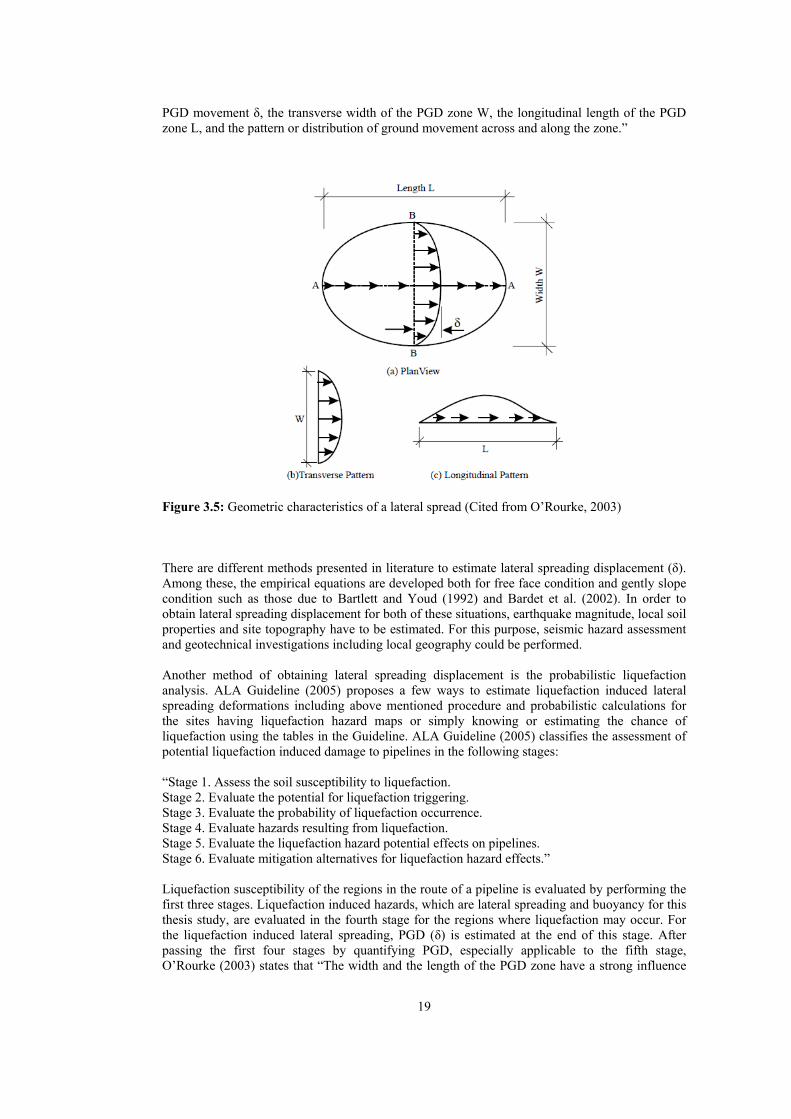
19

PGD movement δ, the transverse width of the PGD zone W, the longitudinal length of the PGD zone L, and the pattern or distribution of ground movement across and along the zone.”

Figure 3.5: Geometric characteristics of a lateral spread (Cited from O’Rourke, 2003) There are different methods presented in literature to estimate lateral spreading displacement (δ). Among these, the empirical equations are developed both for free face condition and gently slope condition such as those due to Bartlett and Youd (1992) and Bardet et al. (2002). In order to obtain lateral spreading displacement for both of these situations, earthquake magnitude, local soil properties and site topography have to be estimated. For this purpose, seismic hazard assessment and geotechnical investigations including local geography could be performed. Another method of obtaining lateral spreading displacement is the probabilistic liquefaction analysis. ALA Guideline (2005) proposes a few ways to estimate liquefaction induced lateral spreading deformations including above mentioned procedure and probabilistic calculations for the sites having liquefaction hazard maps or simply knowing or estimating the chance of liquefaction using the tables in the Guideline. ALA Guideline (2005) classifies the assessment of potential liquefaction induced damage to pipelines in the following stages: “Stage 1. Assess the soil susceptibility to liquefaction. Stage 2. Evaluate the potential for liquefaction triggering. Stage 3. Evaluate the probability of liquefaction occurrence. Stage 4. Evaluate hazards resulting from liquefaction. Stage 5. Evaluate the liquefaction hazard potential effects on pipelines. Stage 6. Evaluate mitigation alternatives for liquefaction hazard effects.” Liquefaction susceptibility of the regions in the route of a pipeline is evaluated by performing the first three stages. Liquefaction induced hazards, which are lateral spreading and buoyancy for this thesis study, are evaluated in the fourth stage for the regions where liquefaction may occur. For the liquefaction induced lateral spreading, PGD (δ) is estimated at the end of this stage. After passing the first four stages by quantifying PGD, especially applicable to the fifth stage, O’Rourke (2003) states that “The width and the length of the PGD zone have a strong influence

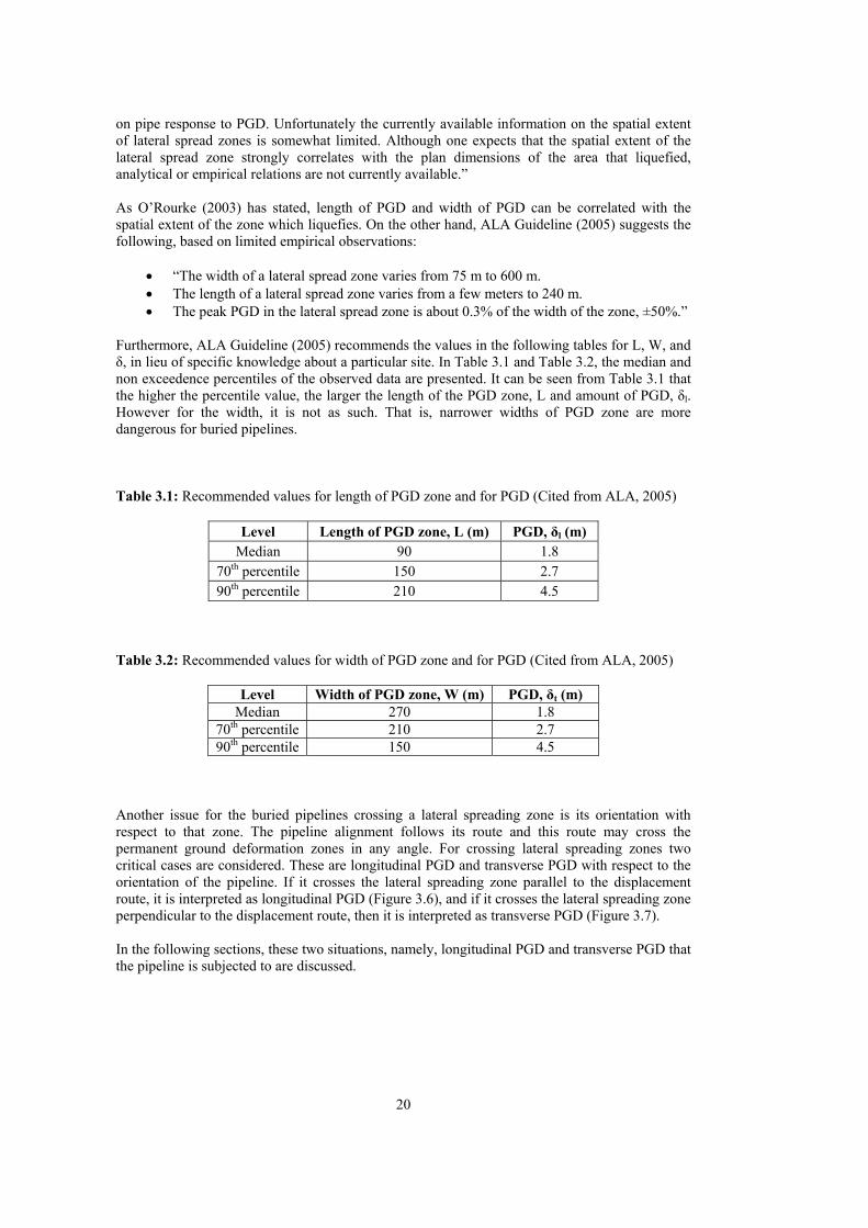
20

on pipe response to PGD. Unfortunately the currently available information on the spatial extent of lateral spread zones is somewhat limited. Although one expects that the spatial extent of the lateral spread zone strongly correlates with the plan dimensions of the area that liquefied, analytical or empirical relations are not currently available.” As O’Rourke (2003) has stated, length of PGD and width of PGD can be correlated with the spatial extent of the zone which liquefies. On the other hand, ALA Guideline (2005) suggests the following, based on limited empirical observations:

“The width of a lateral spread zone varies from 75 m to 600 m. The length of a lateral spread zone varies from a few meters to 240 m. The peak PGD in the lateral spread zone is about 0.3% of the width of the zone, ±50%.”

Furthermore, ALA Guideline (2005) recommends the values in the following tables for L, W, and δ, in lieu of specific knowledge about a particular site. In Table 3.1 and Table 3.2, the median and non exceedence percentiles of the observed data are presented. It can be seen from Table 3.1 that the higher the percentile value, the larger the length of the PGD zone, L and amount of PGD, δl. However for the width, it is not as such. That is, narrower widths of PGD zone are more dangerous for buried pipelines. Table 3.1: Recommended values for length of PGD zone and for PGD (Cited from ALA, 2005)

Level Length of PGD zone, L (m) PGD, δl (m) Median 90 1.8

70th percentile 150 2.7 90th percentile 210 4.5

Table 3.2: Recommended values for width of PGD zone and for PGD (Cited from ALA, 2005)

Level Width of PGD zone, W (m) PGD, δt (m) Median 270 1.8

70th percentile 210 2.7 90th percentile 150 4.5

Another issue for the buried pipelines crossing a lateral spreading zone is its orientation with respect to that zone. The pipeline alignment follows its route and this route may cross the permanent ground deformation zones in any angle. For crossing lateral spreading zones two critical cases are considered. These are longitudinal PGD and transverse PGD with respect to the orientation of the pipeline. If it crosses the lateral spreading zone parallel to the displacement route, it is interpreted as longitudinal PGD (Figure 3.6), and if it crosses the lateral spreading zone perpendicular to the displacement route, then it is interpreted as transverse PGD (Figure 3.7). In the following sections, these two situations, namely, longitudinal PGD and transverse PGD that the pipeline is subjected to are discussed.

Figure 3.6 Figure 3.7

3.3.1.1Pi In order tlength of from geounavailabiextent of displacem One challliquefied aan explanNoshiro observatiodisplayed

6: Longitudin

7: Transverse

ipelineSubje

to evaluate thPGD zone (L

otechnical evaility of an anthe zone wh

ment (δl) can be

lenging unceareas occurredation for this City resultin

ons show that in Figure 3.8

nal PGD (Cited

PGD (Cited f

ectedtoLong

he response oL) and longitudaluations. Al

nalytical or anich liquefies. e obtained fro

rtainty is thed in 1964 Niigsituation. In F

ng from the 20% of the ob(a) (O’Rourk

21

d from GDSM

from GDSMA

gitudinalPGD

of buried condinal permanethough estim

n empirical reBesides, len

om the above m

e pattern of gata and 1983Figure 3.8, lo

1983 Nihonbserved patter

ke, 2003).

1

MA, 2007)

A, 2007)

D

ntinuous pipelent ground de

mating L is elationship, it gth of PGD mentioned pro

deformation. 3 Nihonkai-Chngitudinal PG

nkai-Chubu erns (6 out of 2

lines to longieformation (δl)a challengingcan be correlzone (L) andocedures.

Hamada et hubu earthqua

GD observed aearthquake ar27) have the s

tudinal PGD ) need to be og problem wlated with the

d longitudinal

al. (1986) oakes in order along 5 of 27 re presented.

same general s

effects, obtained with the e spatial

ground

observed to bring lines in

. These shape as

Figure Idealiziby O’Rmodel, followerange (

Figure

e 3.8: Observe

ing the data inRourke et al. (

Ramberg–Oed by the pipeO’Rourke, 20

e 3.9: Block pa

ed longitudina

n Figure 3.8 ((1995) to anasgood type seline, since th

003).

attern of longi

l PGD (Hama

(a), a block paalyze the effecstress–strain rhe failure of t

itudinal PGD

22

ada et al., 1986

attern of longicts of longitudrelation giventhe continuous

(Cited from G

6, as cited from

itudinal PGD dinal PGD to

n in Equations pipeline is t

GDSMA, 2007

m O’Rourke,

(Figure 3.9) i buried pipeli

n 2.4 is assumtypically in th

7)

2003)

is assumed ine. In this med to be he inelastic

23

Figure 3.10: Flowchart for estimating the strain induced by longitudinal PGD (εl)

LONGITUDINAL PGD

Length of PGD zone (L) and longitudinal ground displacement (δl) are obtained

Block pattern is used

Two cases are considered

Case 1: δl is large and pipe strain (εl) is controlled by L

2 1 1 2

Case 2: L is large and pipe strain (εl) is controlled by δl

1 1

1 22 1

Solve effective length (Le) from Estimate εl1 (both tension and compression)

Choose lower as εl

Estimate εl2 (both tension and compression)

24

In this assumption, as can be seen from Figure 3.9, PGD zone, with a length of L and a width of W, is subject to longitudinal permanent ground deformation (δl), which is uniform throughout its length L and 0 out of this zone (O’Rourke, 2003). As it can be followed from the flowchart in Figure 3.10, there are two cases to be considered for a buried pipeline in order to estimate the strain induced by a block pattern of longitudinal PGD. In the first case, longitudinal permanent ground deformation (δl) is large and the pipe strain is controlled by the length (L) of the PGD zone. In the other case, L is large and the pipe strain is controlled by δl (O’Rourke et. al., 1995). The distributions of ground and pipe axial displacements, axial force and axial strain in pipe are shown in Figure 3.11 and Figure 3.12 for cases 1 and 2, respectively.

Figure 3.11: Case 1 - Inelastic model for longitudinal PGD (Cited from O’Rourke et. al., 1995) For both cases, as can be seen from Figure 3.6, there are tension and compression regions for the pipe. While the upper parts of the PGD zone exerts tensile friction forces to the buried pipeline, downwards of the PGD zone exerts compressive friction forces to the buried pipeline. For the case 1, as can be seen from Figure 3.11, from point A to C, buried pipeline is under tension and from point C to E, it is under compression. By symmetry and equilibrium, maximum axial tensile friction force and compressive friction force is tuL/2 at point B and at point D, respectively. Corresponding axial strains, both tensile and compressive, are (GSDMA, 2007, as modified from O’Rourke et al., 1995): 2 1 1 2 3.3

where, L = length of permanent ground deformation zone Sy = yield strength of pipe material

25

n, r = Ramberg-Osgood parameters (see Table 2.1) E = modulus of elasticity of pipe material tu

= peak axial friction force per unit length of pipe at soil pipe interface (see Appendix A) D = outside diameter of pipe t = wall thickness of pipe

Figure 3.12: Case 2 - Inelastic model for longitudinal PGD (Cited from O’Rourke et. al., 1995) For the case 2, as can be seen from Figure 3.12, from point A to C, buried pipeline is under tension, from point D to F, it is under compression. Since L is large, each of tensile and compressive frictional forces acts over an effective length of 2Le. By symmetry and equilibrium, maximum axial tensile friction force and compressive friction force are tuLe at point B and at point E, respectively. In order to estimate corresponding axial strains, effective length, Le, can be estimated from Equation 3.4 which is (GSDMA, 2007, as modified from O’Rourke et al., 1995): 1 22 1 3.4

where, δl = longitudinal permanent ground displacement Le = effective length After that, by substituting Le into Equation 3.5 below, axial tensile and compressive strains can be evaluated as (GSDMA, 2007, as modified from O’Rourke et al., 1995): 1 1 3.5

After the strains are computed for both cases from Equations 3.3 and 3.5, they are compared. For the case 2, L is assumed to be large and as can be seen from Figure 3.12, Le is the distance between points A and B, and also between B and C, which should be less than L/2 due to the underlying assumption. Then, if the computed value of Le from Equation 3.4 is larger than L/2, it

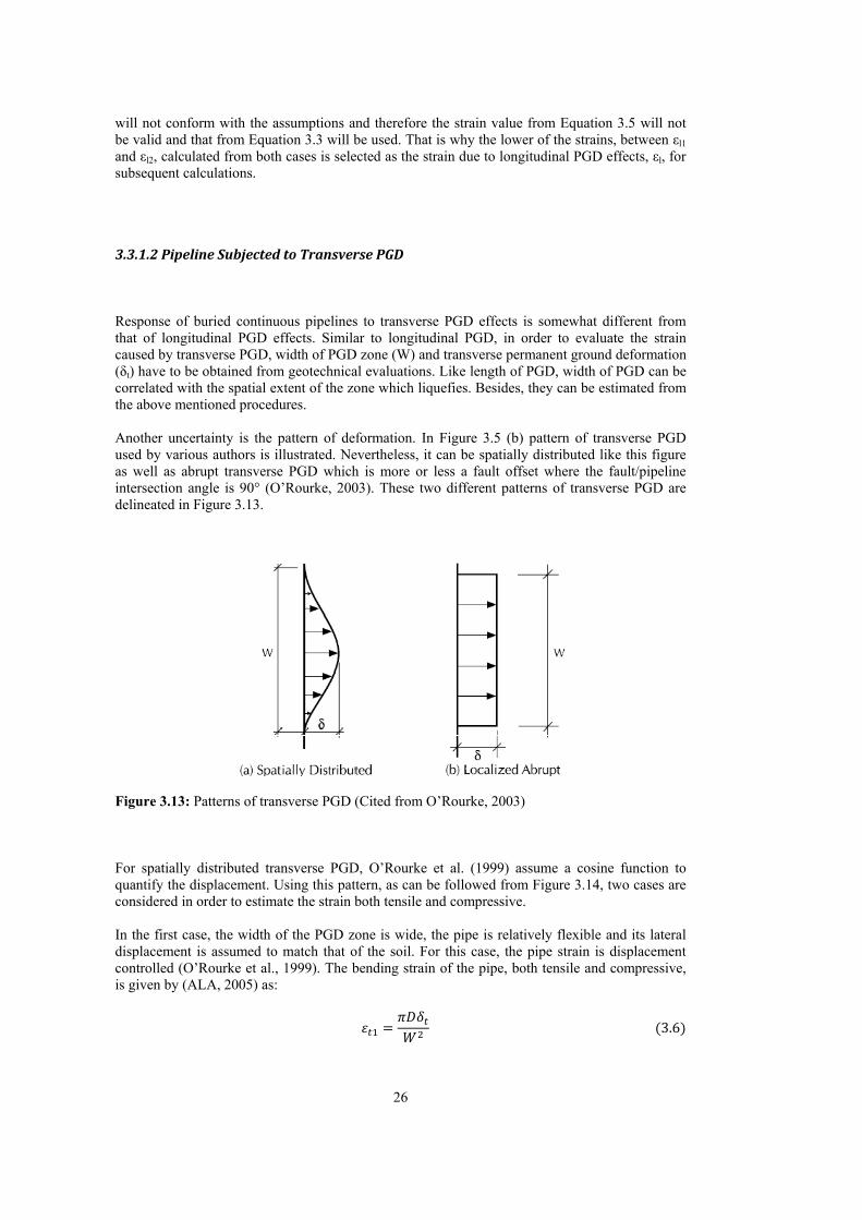
26

will not conform with the assumptions and therefore the strain value from Equation 3.5 will not be valid and that from Equation 3.3 will be used. That is why the lower of the strains, between εl1 and εl2, calculated from both cases is selected as the strain due to longitudinal PGD effects, εl, for subsequent calculations.

3.3.1.2PipelineSubjectedtoTransversePGD Response of buried continuous pipelines to transverse PGD effects is somewhat different from that of longitudinal PGD effects. Similar to longitudinal PGD, in order to evaluate the strain caused by transverse PGD, width of PGD zone (W) and transverse permanent ground deformation (δt) have to be obtained from geotechnical evaluations. Like length of PGD, width of PGD can be correlated with the spatial extent of the zone which liquefies. Besides, they can be estimated from the above mentioned procedures. Another uncertainty is the pattern of deformation. In Figure 3.5 (b) pattern of transverse PGD used by various authors is illustrated. Nevertheless, it can be spatially distributed like this figure as well as abrupt transverse PGD which is more or less a fault offset where the fault/pipeline intersection angle is 90° (O’Rourke, 2003). These two different patterns of transverse PGD are delineated in Figure 3.13.

Figure 3.13: Patterns of transverse PGD (Cited from O’Rourke, 2003) For spatially distributed transverse PGD, O’Rourke et al. (1999) assume a cosine function to quantify the displacement. Using this pattern, as can be followed from Figure 3.14, two cases are considered in order to estimate the strain both tensile and compressive. In the first case, the width of the PGD zone is wide, the pipe is relatively flexible and its lateral displacement is assumed to match that of the soil. For this case, the pipe strain is displacement controlled (O’Rourke et al., 1999). The bending strain of the pipe, both tensile and compressive, is given by (ALA, 2005) as: 3.6

27

Figure 3.14: Flowchart for estimating the strain induced by transverse PGD (εt)

TRANSVERSE PGD

Width of PGD zone (W) and transverse ground displacement (δt) are obtained

Cosine function is used as pattern of PGD


Case 1: Wide W and pipe is assumed to be flexible

Case 2: Narrow W and pipe is assumed to be stiff

3

Estimate bending strain (εt1) (both tension and compression)

Choose lower as εt

Estimate bending strain (εt2) (both tension and compression)

28

where, D = outside diameter of pipe δt = transverse permanent ground deformation W = width of permanent ground deformation zone In the other case, the width of the PGD zone is narrow, the pipe is relatively stiff and the pipe lateral displacement is assumed as loading controlled since the soil displacement is much higher than that of the pipe. For this fixed-fixed beamlike behaviour, the bending strain of the pipe, both tensile and compressive, is given by the following equation (O’Rourke et al., 1999): 3 3.7

where, Pu = maximum lateral resistance of soil per unit length of pipe (see Appendix A) E = modulus of elasticity of pipe material More detailed information on Pu is presented in Appendix A. For both conditions axial strains are neglected because of their small magnitude. After computing both strains, εt1 and εt2, by using Equations 3.6 and 3.7, they are compared. Strain computed from Equation 3.7 should be less than that computed from Equation 3.6 because strain computed from Equation 3.7 is based on the assumption that the pipe is stiff and therefore exhibits smaller deformation compared to soil deformation. On the other hand, for a same width of PGD, strain computed from Equation 3.6 is based on the assumption that pipe is flexible and exhibits similar deformation compared to soil deformation, which results in larger strain estimates than the strain computed from Equation 3.7. Thus, if the strain computed from Equation 3.7 is larger than that from Equation 3.6, this will not be acceptable. That is why the lower of εt1 or εt2, denoted by εt, is used as the strain due to transverse PGD effects.

3.3.2LiquefactionInducedBuoyancy Liquefaction induced buoyancy effects can be considered when the soil layer, in which the pipeline is buried, liquefies. ALA Guideline (2005) reports that “pipe damage to sewer pipes due to buoyancy has been commonly observed in a variety of earthquakes in Japan.” Since sewer pipes are buried in deeper depths, maximum displacement caused by buoyancy is increased. Also they were segmented pipes, as a result it is concluded that buoyancy caused pipe failures in Japan earthquakes. On the other hand, for continuous pipelines, buried at shallow depths, buoyancy induced pipe strains might be small, which do not cause failure. In such a situation, pipelines float and may uplift out of the ground surface due to buoyancy and this can be interpreted as a serviceability limit state, since pipelines are buried for aesthetics and safety. Buoyancy strains for buried pipelines can be estimated in a procedure similar to that of the transverse PGD. While transverse PGD occurs in horizontal plane, buoyancy effects take place in vertical plane. In both situations, buried pipelines are under the effects of bending strains, and axial strains are small enough to be neglected. The flowchart describing the procedure for strain estimation of buried continuous pipelines subject to liquefaction induced buoyancy effects is illustrated in Figure 3.15.

29

4

BUOYANCY

Length of buoyancy zone (Lb) is obtained

Cosine function is used as pattern of PGD


Case 2: Large Lb and pipe is assumed to be flexible

Case 1: Narrow Lb and pipe is assumed to be stiff

1 1

Estimate tensile (+εb2t) and compressive (-εb2c) strains

Choose lower as εb

Estimate tensile (+εb1) and compressive (-εb1) strains

4

10

Figure 3.15: Flowchart for estimating the strain induced by liquefaction induced buoyancy (εb)

30

In this procedure, first, length of buoyancy zone (Lb) (illustrated in Figure 3.16) should be assessed to estimate the strain in the buried pipeline. It can be obtained from geotechnical investigations performed for the assessment of local soil conditions in examining the liquefaction potential. That is, Lb will be similar to the dimensions of the liquefaction induced lateral spread. In other words, the length of the pipeline buried in the liquefied zone corresponds to the length of the buoyancy zone.

Figure 3.16: Longitudinal section of the pipeline showing the forces acting on it due to buoyancy (ALA, 2001, as cited from GDSMA, 2007) Two cases are considered in this procedure similar to that of transverse PGD. In the first case, the length of buoyancy zone is narrow, the pipeline is relatively stiff and the pipe’s vertical displacement is assumed to be due to loading at the soil-pipe interface (O’Rourke et al., 1999). For this fixed-fixed beamlike behaviour, the stress estimation procedure is explained in ALA Guideline (2001). However, as can be seen from Figures 3.16 and 3.17, ALA Guideline (2001) put forward the buoyancy forces when the pipeline is buried under water table, compared to liquefaction induced buoyancy. In the Guideline, “The upward force imposed on a straight, buried, welded carbon-steel pipe from the water table being above the pipe is”: 3.8 where: Fb = upward force due to buoyancy per unit length of pipe Ww = weight of water displaced by pipe per unit length of pipe Wp = weight of pipe per unit length of pipe Wc = weight of pipe contents per unit length of pipe Pv = earth pressure γw = unit weight of water hw = water level from top of pipe D = outside pipe diameter When liquefaction induced buoyancy is considered, the following formula is used (O’Rourke et al., 1999): 4 3.9

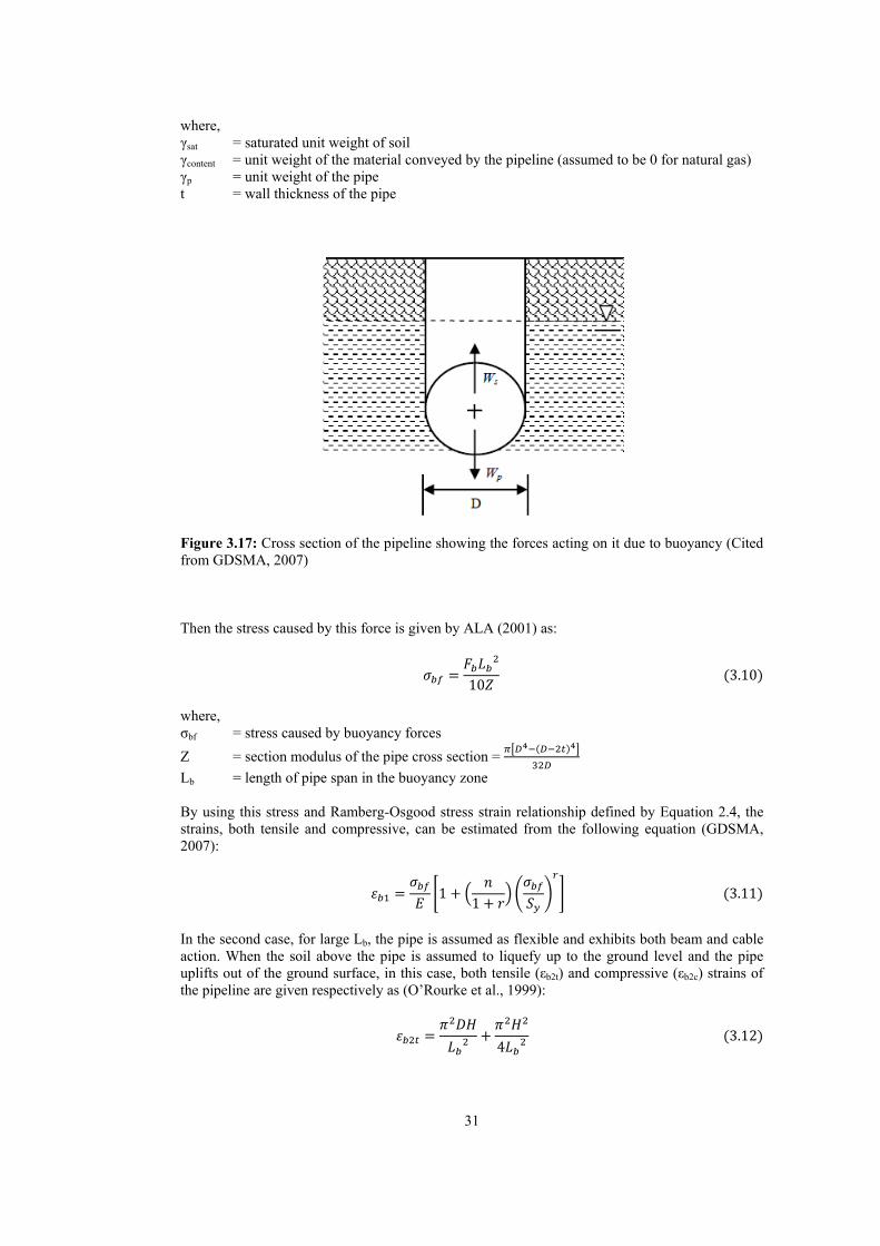
31

where, γsat = saturated unit weight of soil γcontent = unit weight of the material conveyed by the pipeline (assumed to be 0 for natural gas) γp = unit weight of the pipe t = wall thickness of the pipe

Figure 3.17: Cross section of the pipeline showing the forces acting on it due to buoyancy (Cited from GDSMA, 2007) Then the stress caused by this force is given by ALA (2001) as: 10 3.10

where, σbf = stress caused by buoyancy forces

Z = section modulus of the pipe cross section =

Lb = length of pipe span in the buoyancy zone By using this stress and Ramberg-Osgood stress strain relationship defined by Equation 2.4, the strains, both tensile and compressive, can be estimated from the following equation (GDSMA, 2007): 1 1 3.11

In the second case, for large Lb, the pipe is assumed as flexible and exhibits both beam and cable action. When the soil above the pipe is assumed to liquefy up to the ground level and the pipe uplifts out of the ground surface, in this case, both tensile (εb2t) and compressive (εb2c) strains of the pipeline are given respectively as (O’Rourke et al., 1999): 4 3.12

32

4 3.13

where, D = diameter of the pipe H = depth of burial from center of the pipe to the ground surface Lb = length of pipe span in the buoyancy zone After finding the strains from Equations 3.11 and 3.12, they are compared. Based on the same reasons with transverse PGD (stiff-flexible pipe and soil interaction), strain computed from Equation 3.11 (εb1) should be less than that computed from Equation 3.12 (εb2t) for the same length of buoyancy zone (Lb). In this comparison, εb2c is not considered to be on safe side since the local buckling failure mode is more critical for buried continuous pipelines. Thus, if the strain computed from Equation 3.11 is larger than that from Equation 3.12, this will not be valid. That is why the lower of the strains computed from Equations 3.11 and 3.12 is taken as the buoyancy strain (εb) in the reliability computations.

3.3.3FaultCrossing One of the most important factors to be considered in the seismic design of buried pipelines is fault crossing. From the past observed earthquakes, its detrimental effect has been recorded drastically. For example, during the 1971 San Fernando earthquake, although surface faulting regions were very small compared to the shaken area, due to the fault movements, over 1400 breaks in water, natural gas, and sewer pipelines occurred (McCaffrey and O’Rourke, 1983). On account of these detrimental effects, buried pipelines, which intersect active faults, should be designed accordingly. Active fault displacements are the results of earth crust’s relative movements and it can be met in different forms in terms of directivity. The principal types of fault movements are normal, reverse and strike slip. While normal and reverse fault movements are occurring in vertical plane, strike slip fault movements occur in horizontal plane. For normal faults, buried pipeline is primarily under tension. Yet for the reverse faults, it is primarily under compression. For strike slip faults, the behavior is dependent on fault crossing angle. There are two modes of behavior for a buried pipeline crossing a fault depending on the fault type and crossing angle. First is the tensile failure of the pipeline. For normal and strike slip faults, when the pipe-fault intersection angle β, as shown in Figure 3.18, is less than 90°, buried pipelines are subject to bending forces due to the transverse component of fault offset and axial tensile forces due to the longitudinal component of fault offset. This can cause tensile failure of the pipelines by excessive displacements. Second mode of behaviour is buckling failure due to compressive forces. For reverse and strike slip faults when the pipe-fault intersection angle β is greater than 90°, buried pipelines are subject to axial compressive forces due to the longitudinal component of fault offset (O’Rourke, 2003). In the analysis of pipelines crossing active faults, fault displacements should be estimated. It can be obtained from displacement-moment magnitude relationships such as those provided by Wells and Coppersmith (1994). ALA Guideline (2005) recommends this method as well as some probabilistic methods in order to quantify fault displacement. Also states that: “Fault offset can also be estimated by using historical evidence, paleoseismic evidence and/or slip rate calculations.”

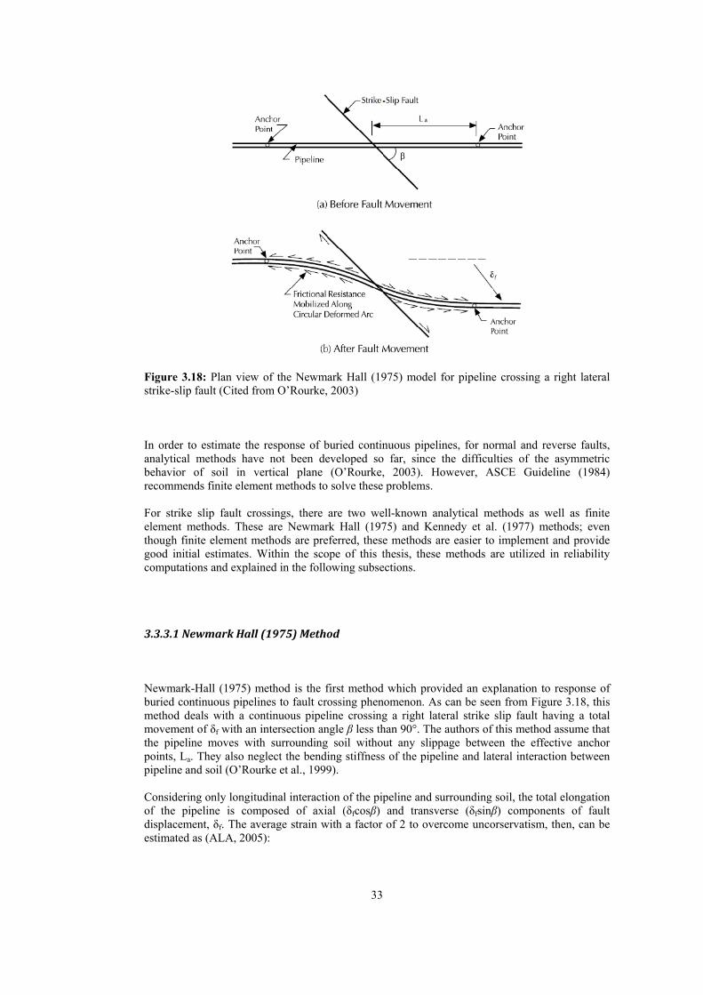
33

Figure 3.18: Plan view of the Newmark Hall (1975) model for pipeline crossing a right lateral strike-slip fault (Cited from O’Rourke, 2003) In order to estimate the response of buried continuous pipelines, for normal and reverse faults, analytical methods have not been developed so far, since the difficulties of the asymmetric behavior of soil in vertical plane (O’Rourke, 2003). However, ASCE Guideline (1984) recommends finite element methods to solve these problems. For strike slip fault crossings, there are two well-known analytical methods as well as finite element methods. These are Newmark Hall (1975) and Kennedy et al. (1977) methods; even though finite element methods are preferred, these methods are easier to implement and provide good initial estimates. Within the scope of this thesis, these methods are utilized in reliability computations and explained in the following subsections.

3.3.3.1NewmarkHall(1975)Method Newmark-Hall (1975) method is the first method which provided an explanation to response of buried continuous pipelines to fault crossing phenomenon. As can be seen from Figure 3.18, this method deals with a continuous pipeline crossing a right lateral strike slip fault having a total movement of δf with an intersection angle β less than 90°. The authors of this method assume that the pipeline moves with surrounding soil without any slippage between the effective anchor points, La. They also neglect the bending stiffness of the pipeline and lateral interaction between pipeline and soil (O’Rourke et al., 1999). Considering only longitudinal interaction of the pipeline and surrounding soil, the total elongation of the pipeline is composed of axial (δfcosβ) and transverse (δfsinβ) components of fault displacement, δf. The average strain with a factor of 2 to overcome uncorservatism, then, can be estimated as (ALA, 2005):

34

Figure 3.19: Flowchart for estimating the strain due to fault crossing effects by using Newmark Hall (1975) method (εNH)

FAULT CROSSING (Newmark & Hall (1975) approach,

for strike slip fault)

Magnitude (M) and corresponding fault displacement (δf) are obtained

Fault crossing angle (β) is estimated

Axial (tu) soil force is estimated

Unanchored pipe length (La) is estimated

′ 1 2 tan ′

2 2 12 2

Estimate εNH

Use εNH

Actual La

Take minimum

of

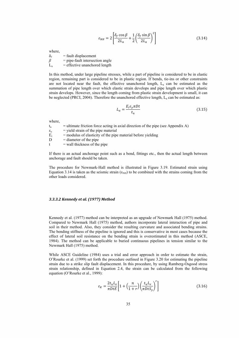
35

2 cos2 12 sin2 3.14

where, δf = fault displacement β = pipe-fault intersection angle La = effective unanchored length In this method, under large pipeline stresses, while a part of pipeline is considered to be in elastic region, remaining part is considered to be in plastic region. If bends, tie-ins or other constraints are not located near the fault, the effective unanchored length, La can be estimated as the summation of pipe length over which elastic strain develops and pipe length over which plastic strain develops. However, since the length coming from plastic strain development is small, it can be neglected (PRCI, 2004). Therefore the unanchored effective length, La can be estimated as: 3.15

where, tu = ultimate friction force acting in axial direction of the pipe (see Appendix A) εy = yield strain of the pipe material Ei = modulus of elasticity of the pipe material before yielding D = diameter of the pipe t = wall thickness of the pipe If there is an actual anchorage point such as a bend, fittings etc., then the actual length between anchorage and fault should be taken. The procedure for Newmark-Hall method is illustrated in Figure 3.19. Estimated strain using Equation 3.14 is taken as the seismic strain (εNH) to be combined with the strains coming from the other loads considered.

3.3.3.2Kennedyetal.(1977)Method Kennedy et al. (1977) method can be interpreted as an upgrade of Newmark Hall (1975) method. Compared to Newmark Hall (1975) method, authors incorporate lateral interaction of pipe and soil in their method. Also, they consider the resulting curvature and associated bending strains. The bending stiffness of the pipeline is ignored and this is conservative in most cases because the effect of lateral soil resistance on the bending strain is overestimated in this method (ASCE, 1984). The method can be applicable to buried continuous pipelines in tension similar to the Newmark Hall (1975) method. While ASCE Guideline (1984) uses a trial and error approach in order to estimate the strain, O’Rourke et al. (1999) set forth the procedure outlined in Figure 3.20 for estimating the pipeline strain due to a strike slip fault displacement. In this procedure, by using Ramberg-Osgood stress strain relationship, defined in Equation 2.4, the strain can be calculated from the following equation (O’Rourke et al., 1999): 2 1 1 3.16

36

FAULT CROSSING (Kennedy et. al (1977) approach,

for strike slip fault)

Magnitude (M) and corresponding fault displacement (δf) are obtained

Fault crossing angle (β) is estimated

Axial (tu) and lateral (Pu) soil forces are estimated

Total elongation (ΔL) is estimated

′ 1 2 tan ′

2 1 1

Solve effective length (Le) from

∆ 1 22 1

Estimate εK (tensile)

′

∆ cos sin3

Use εK

sin

Figure 3.20: Flowchart for estimating the strain due to fault crossing effects using Kennedy et al. (1977) method (εK)

37

where, Le = effective length Sy = yield stress of pipe material n, r = Ramberg-Osgood parameters (to be obtained from Table 2.1) E = modulus of elasticity of pipe material tu

= peak friction force per unit length of pipe at soil pipe interface (see Appendix A)

D = outside diameter of pipe t = wall thickness of pipe Similar to estimating the strain developed due to longitudinal PGD, an effective length Le should be assessed in order to estimate the strain. To find this length, first the total elongation of the pipe is estimated from: ∆ cos sin3 3.17

where, ΔL = total elongation of the pipe δf = fault displacement β = pipe-fault intersection angle Lc = the horizontal projection of the laterally deformed pipe (see Figure 3.21)

Figure 3.21: Kennedy et al. (1977) model (as given in O’Rourke et al., 1999) In this equation, while the first term is due to the axial component of the fault displacement, the second is due to the arc length effects caused by lateral component of the fault displacement. The unknown parameter, Lc can be estimated from: sin 3.18

where Rc is the radius of curvature, seen in Figure 3.21, and can be computed from: 3.19

where, σ = the axial stress at fault crossing, Pu = the lateral soil–pipe interaction force per unit length (see Appendix A)

Rc

Pu

tu δfsinβ/2

Lc

38

ΔL can also be expressed as follows (O’Rourke et al., 1999): ∆ 1 22 1 3.20

Equating Equations 3.17 and 3.20, Le can be estimated. Le is then inserted into Equation 3.16 and seismic tensile strain due to strike slip fault crossing effects (εK) is estimated. The computed value can be interpreted as a good approximate of the one that will be obtained from the finite element method (O’Rourke et al., 1999).

39

CHAPTER4

STRUCTURALRELIABILITYASSESSMENTOFBURIEDPIPELINES

4.1Introduction From structural reliability point of view, there are two states for a structure. If the structure fulfills its function, it survives, otherwise it fails. This can be at its ultimate limit state, serviceability limit state or accidental limit state, etc. So as to assess the survival and failure probabilities of structures and utilize this differentiation in various stages, such as design, insurance, etc., probabilistic methods have been developed over the last 60 years. These methods are based on the probability of failure or the probability of the complementary event (i.e. survival), called reliability. In the probabilistic approach uncertainty quantification is quite important. None of the load and resistance parameters can be quantified exactly. Accordingly, probabilistic methods deal with these uncertainties by treating the basic variables as random variables. Using random variables, reliability can also be expressed based on the concept of the reliability index, β which is first introduced by Cornell (1969), and improved and modified later by Hasofer and Lind (1974). The methods they use are the first order second moment (FOSM) methods, and reliability index is the usual output of these methods. For this purpose, failure modes and corresponding limit states need to be identified. After that probability of failure or survival can be estimated for each failure mode. For buried continuous pipelines, tensile and local buckling failure modes are critical depending on the type of loading. Loads due to internal pressure and temperature changes and earthquake induced loads described in the previous chapters are taken into consideration in reliability calculations. In this chapter, the basic concepts of structural reliability are presented and reliability analysis for buried continuous pipelines subject to earthquake effects is performed.

4.2StructuralReliabilityMethods

4.2.1TheClassicalReliabilityFormulation

40

Structural reliability deals with the interaction of capacity and demand. Capacity or the resistance, R, of a structure should be large enough to carry the applied load, S to be able to sustain its function. In terms of reliability of a single member, failure occurs when R is less than S. Or it can be expressed by introducing the safety margin, M, which is expressed as: 4.1 When M<0, failure takes place and probability of failure, Pf, can be defined as: 0 4.2 where P(.) is the probability of occurrence of the event in brackets. If R and S are statistically independent and normally distributed, with mean values of µR and µS, and standard deviations of σR and σS, respectively, the probability of failure becomes: 1 Φ 1 Φ 4.3

where, Φ(.) = cumulative standard normal probability distribution function µM = mean value of the safety margin σM = standard deviation of safety margin Then the reliability, Ps, is defined as the probability of non-failure or probability of survival, which is given as follows: 1 Φ Φ 4.4

4.2.2FirstOrderSecondMomentMethod The reliability is the survival probability of the structure during its lifetime. To be able to formulize this, limit states need to be determined and corresponding limit state functions are formed by introducing load and resistance parameters (Ellingwood et. al., 1980). These load and resistance parameters are called basic variables. By inputting these variables, the safety margin, M, can be defined in terms of the limit state on failure function as: , . . . , 4.5 where, X = the vector of basic variables Then the failure surface becomes: , . . . 0 4.6 As illustrated in Figure 4.1, when 0, the corresponding set of basic variables are in the safe region, Ds, otherwise in the failure region, Df, (Thoft-Christensen and Baker, 1982).

41

Figure 4.1: Failure surface and reliability index, βHL (Modified from Thoft-Christensen and Baker, 1982) Cornell (1969) introduced the reliability index, βc, defined as follows: 4.7

Reliability index, βc, accounts for the level of expected performance of the structure in the corresponding limit state and the larger the value it has, the safer will be the structure and the higher its performance, as can also be seen from Table 4.1. Table 4.1: Relationship between reliability index (β), probability of failure and expected performance level for normally distributed basic variables and linear failure functions (Cited from US Army Corps of Engineers, 1997)

Reliability Index(β)

Probability of FailurePf= Φ(-β)

Expected Performance Level

1.0 0.16 Hazardous 1.5 0.07 Unsatisfactory 2.0 0.023 Poor 2.5 0.006 Below average 3.0 0.001 Above average 4.0 0.00003 Good 5.0 0.0000003 High

If the safety margin M is linear in the basic variables X1,…, Xn, as shown in Equation 4.8: ⋯ 4.8 Then the mean and variance of M are as follows:

42

⋯ 4.9 ⋯ 4.10

where, a0,...,an = constants µi = mean of the ith basic variable σi = standard deviation of the ith basic variable ρij = correlation coefficient between basic variables Xi and Xj For linear failure functions, above equations can be used. However for nonlinear failure functions, there are methods developed to estimate mean and variance of the safety margin. Mean value and advanced first order second moment (AFOSM) methods are discussed in the following sections.

4.2.2.1MeanValueMethod For a nonlinear failure function, the safety margin, M, µM and σM can be estimated approximately by using Taylor Series expansion. If Equation 4.5 is expanded about mean vector of basic variables, μ , and if higher order terms are neglected and only the linear terms are kept, then safety margin, M, becomes: ≅ , . . . , ,..., 4.11

Mean and variance of the safety margin, M, can be approximated as: ≅ , . . . , 4.12 ≅ ,..., ,..., ,..., 4.13

where, COVij = covariance between Xi and Xj This method, which is widely known as the First Order Second Moment (FOSM) method, is easy to use especially with a computer to be able to calculate complex mathematical operations, e.g. derivatives. However, it has two basic shortcomings which Ellingwood et al. (1980) pointed out as: 1. If the failure function is nonlinear, significant errors may be introduced at increasing

distances from the linearized point by neglecting higher order terms. 2. The mean value method fails to be invariant to different mechanically equivalent

formulations of the same problem. In effect, this means that reliability index depends on how the limit state is formulated. This is a problem not only for nonlinear forms of failure functions but even in certain linear forms, e.g., when the loads counteract one another.

43

In this context, Advanced First Order Second Moment (AFOSM) method is introduced to solve these shortcomings described as follows.

4.2.2.2AdvancedFirstOrderSecondMomentMethod The above mentioned unsatisfactory condition of the mean value method can be solved by Advanced First Order Second Moment (AFOSM) method whose pioneers are Hasofer and Lind (1974). This method is also referred to as the First Order Reliability Method (FORM) in recent years. They introduced a modified reliability index, βHL, which is defined as the nearest point of estimate of the limit state function to the origin of a standard Gaussian space (see Figure 4.1). In order to estimate βHL, basic variables forming the limit state function should be normalized to have zero mean and unit variance as follows: , 1,2, … , 4.14

By transforming Xi’s into Zi’s, the coordinate space and corresponding limit state function are changed. New coordinate system, Z, as can be seen for the two basic variables in Figure 4.1, is now the subject of interest. In this coordinate system, βHL is the shortest distance between the limit state function and origin, and the intersection point of that distance vector and limit state function is referred to as the design point. From this point of view, βHL can be expressed as: / 4.15 → : ∈ where,

= vector of normalized basic variables = limit state (failure) surface in the z-coordinate system

For the nonlinear limit state functions, reliability index, βHL, and design point can be solved iteratively by using the equations below (Thoft- Christensen and Baker, 1982):

∑ , 1,2, … , 4.16

∗ 4.17 ∗, . . . , ∗ 0 4.18 where, αi = directional cosines that minimizes βHL Zi

* = ith component of design point

44

If random variables are correlated, in order to perform this iterative procedure, all variables should be transformed into uncorrelated variables. This is achieved by deriving from covariance matrix, CX, and mean vector, μ , uncorrelated covariance matrix, CY, and uncorrelated mean vector, μ , as follows (Thoft- Christensen and Baker, 1982): μ μ 4.19 C A 4.20 where, A = matrix composed of orthonormal eigenvectors of CX

4.3CombinationofFailureModes Structures may fail in different failure modes. These failure modes are usually more than one for a structure. For instance, for buried continuous pipelines tensile rupture and buckling failure modes are usually encountered. Generally different failure modes may be correlated. In order to evaluate the reliability of structures, these different failure modes should be considered jointly. Let a structural component has k failure modes, which are denoted as E1, E2,…, Ek. Each failure mode has its own limit state function and individual failure event corresponding to the ith failure mode is as follows (Ang and Tang, 1984): 0 4.21 where,

= limit state function of the ith failure mode Then the compliment of is the individual safe event, , which is expressed as: 0 4.22 Survival of the system is the event, , in which all individual safe events occur at the same time. That is: ∩ ∩ … ∩ 4.23 Conversely, the failure event, , is as follows: ∪ ∪ … ∪ 4.24 where, ∩ and ∪ denote, intersection and union of events, respectively. Let S be the load acting on the structure concerned and Ri is the capacity of a certain component in the ith failure mode. If modal capacities are dependent on each other but are independent on load, S, then the survival probability becomes (Yücemen, 2006): … ,…, , … , … 4.25

45

where, … = load effects in different failure modes ,…, , … , = joint probability density function of k-modal resistances = probability density function of load

Since the calculation of the probability of survival from Equation 4.25 is rather difficult, bounds are formed to estimate the survival probability as explained below (Yücemen, 2006):

a) In setting up the first bound, failure modes are assumed to be perfectly correlated. In this situation, probability of survival, , is the minimum of the survival probabilities of each failure mode, which is expressed as follows: min , , … , 4.26 where, is the survival probability of ith failure mode, which can be computed from the following equation: Pr 4.27

b) In establishing the second bound, k modal resistances are assumed to be statistically

independent, loads are still dependent. Then, probability of survival, , becomes: … 4.28

Or it can be expressed as follows:

Pr Pr … Pr 4.29

c) In obtaining the last bound, modal resistances and modal loads in different modes are

assumed to be statistically independent. That is, failure modes are independent. In this case probability of survival, ∗, becomes as the product of the survival probabilities of each failure mode, which is expressed as follows:

∗ 4.30

After these bounds are determined, fundamental inequalities of reliability can be utilized as described below: ∗ 4.31 Or, in terms of failure probabilities: ∗ 4.32 where, , = survival and failure probabilities of a component, respectively, corresponding to

perfectly correlated failure modes

46

, = true values of survival and failure probabilities of a component, respectively , = survival and failure probabilities of a component, respectively, corresponding to independent modal resistances but dependent loads ∗, ∗ = survival and failure probabilities of a component, respectively, corresponding to independent failure modes

4.4UncertaintyModeling In order to perform a reliability analysis, the uncertainties of each random variable need to be determined. This can be attained by using variance, standard deviation or coefficient of variation (c.o.v.). More accurate results will be obtained if the uncertainties and variabilities are of small magnitude. Therefore uncertainties should be reduced as much as possible. Yet, uncertainties are involved both in the basic variables forming the corresponding limit state function, and in the prediction model used in forming the limit state function. To account for these uncertainties, two kinds of uncertainties are defined in structural engineering. These are aleatory and epistemic uncertainties. Aleatory uncertainty results from inherent variability and cannot be reduced by additional information or data. On the other hand, epistemic uncertainty, which results from lack of sufficient knowledge or information, can be reduced by additional information and data. There are three sources of epistemic uncertainties. These are prediction, modeling and statistical errors. Prediction uncertainty can be exemplified as the discrepancies between in-situ and laboratory conditions. Modeling uncertainty is the uncertainties related with the assumptions, approximations, idealization of real situations like plain strain analysis instead of 3-D analysis. Statistical uncertainty, results from the lack of sufficient number of observations to quantify the mean of a random variable. All sources of information should be utilized in order to reduce these uncertainties. These sources of uncertainties can be reduced by additional data and expert opinion. The different sources of uncertainties can be combined with the model presented as follows (Ang and Tang, 1984): N X 4.33 where, Xi = true (but unknown) value of the ith basic variable Ni = random correction factor to account for epistemic uncertainties X = model used to estimate Xi By using First Order Second Moment method (Equations 4.11 and 4.12), the mean and total uncertainty of the ith basic variable can be formulated as: N X 4.34 Ω Δ 4.35

where, µXi = mean value of the ith basic variable N = mean bias of the ith basic variable

47

X = mean value of the model used to estimate the ith basic variable ΩXi = total uncertainty of the ith basic variable

= coefficient of variation quantifying the aleatory uncertainty (inherent variability) of the ith basic variable Δ = coefficient of variation quantifying the epistemic uncertainty of the ith basic variable

Let Ni be the product of n component correction factors as follows: … 4.36 Then assuming all Ni’s to be mutually independent, mean bias and coefficient of variation quantifying the epistemic uncertainty of the ith basic variable can be written by using FOSM approximation as follows: N … 4.37 Δ Δ Δ ⋯ Δ 4.38

Within the scope of this thesis, uncertainties associated with basic variables are obtained from various sources and listed in Table 4.2 and Table 4.3. For the sake of convenience all random variables are assumed to be normally distributed. Please also note that some of the values given here are valid specifically for the case studies to be presented in the next chapter. For the definition of the symbols used to denote the basic variables, please refer to the previous sections or “List of Symbols and Abbreviations” section. Also for the notation of soil types, please refer to the Appendix B.

4.5IdentificationandDescriptionofDifferentFailureModes Steel pipelines manufactured from ductile material possess high ductility and may fracture at about 20% elongations when loaded in tension. With fully penetrated arc butt welds at joints, their performance goes well beyond segmented pipelines. Nevertheless, continuous pipelines should accommodate high strains due to PGD and other earthquake effects. Since the deformations are beyond the elastic limit of pipelines, the ductility advantage of continuous pipelines need to be used in earthquake resistant design. Thus, strain limits are developed for the failure modes. There are three main types of failure modes for corrosion-free continuous pipelines. These are tensile failure, local buckling and beam buckling. The first two of these are common failure modes. On the other hand, beam buckling is not prevalent because beam buckling occurs at shallow burial depths which are generally below the typical burial depths of pipelines. In only shallow depths of burial, less than about 90 cm, pipelines may experience this type of behavior. Accordingly, this type of failure mode is not considered in this study.

48

Table 4.2: Mean values and coefficients of variation quantifying the aleatory uncertainties of basic variables

Basic Variables mean c.o.v. Reference

Sy (MPa)

475 0.10 Amirat et al. (2006)

400 0.05 Ahammed et al. (1997)

358 0.07 Caleyo et al. (2002)

423 0.067 Ahammed (1998)

275.79 0.07 Michalopoulos et al. (2000)

1.1SMYS 0.035 Chen et al. (2001)

D (mm)

914.4 0.02 Caleyo et al. (2002)

600 0.03 Ahammed (1998)


nominal 0.0006 Chen et al. (2001)

ri (mm) 97.3 0.10 Amirat et al. (2006)

225 0.04 Ahammed et al. (1997)

t (mm)

12.7 0.05 Amirat et al. (2006)

7 0.06 Ahammed et al. (1997)

20.6 0.02 Caleyo et al. (2002)

10 0.05 Ahammed (1998)


nominal 0.01 Chen et al. (2001)

P (MPa)

7 0.10 Amirat et al. (2006)

5 0.10 Ahammed et al. (1997)

7.8 0.10 Caleyo et al. (2002)

5 0.10 Ahammed (1998)


ν 0.283 0.023 Amirat et al. (2006)

0.3 0.023 Ahammed et al. (1997)

E (MPa) 201000 0.04 Amirat et al. (2006)

201000 0.033 Ahammed et al. (1997)

αt (1/oC) 1.17E-05 0.10 Amirat et al. (2006)

1.17E-05 0.10 Ahammed et al. (1997)

ΔT (oC) 10 0.15 Amirat et al. (2006)

10 0.15 Ahammed et al. (1997)

H (mm) 1657 0.10 BOTAŞ Specifications (2000)

L (mm) 90000 1.15 ALA (2005)

δl (mm) 1800 1.06 ALA (2005)

W (mm) 270000 0.38 ALA (2005)

δt (mm) 1800 1.06 ALA (2005)

49

Table 4.2 (Cont’d)

Basic Variables mean c.o.v. Reference

Lb (mm) 270000 0.38 ALA (2005)

δf (mm) Wells and Coppersmith (1994)

β (o) 90 0.10

φ (o)

0.02-0.13 Duncan (2000)

Soil Type

CL 26.50 0.19 Loehr et al. (2005)

CH 21.80 0.27 Loehr et al. (2005)

ML 30.50 0.11 Loehr et al. (2005)

CL-ML 27.20 0.15 Loehr et al. (2005)

γ' (N/mm3)

1.89E-05 0.10 Amirat et al. (2006)

1.89E-05 0.10 Ahammed et al. (1997)

Soil Type

GP-GW 0.14-0.18 Gutierrez et al. (2003)

SM-ML 0.14-0.35 Gutierrez et al. (2003)

SP-SW 0.20 Gutierrez et al. (2003)

γsat (N/mm3)

0.03-0.07 Duncan (2000)

Soil Type

CL 1.93E-05 0.03 Loehr et al. (2005)

CH 1.88E-05 0.03 Loehr et al. (2005)

ML 1.94E-05 0.05 Loehr et al. (2005)

CL-ML 1.99E-05 0.03 Loehr et al. (2005)

GP-GW 0.07-0.09 Gutierrez et al. (2003)

SM-ML 0.06-0.12 Gutierrez et al. (2003)

SP-SW 0.09 Gutierrez et al. (2003)

c (MPa)

0.13-0.40 Duncan (2000)

Soil Type

CL 0.038 0.49 Loehr et al. (2005)

CH 0.066 0.37 Loehr et al. (2005)

ML 0.029 0.64 Loehr et al. (2005)

CL-ML 0.028 0.61 Loehr et al. (2005)

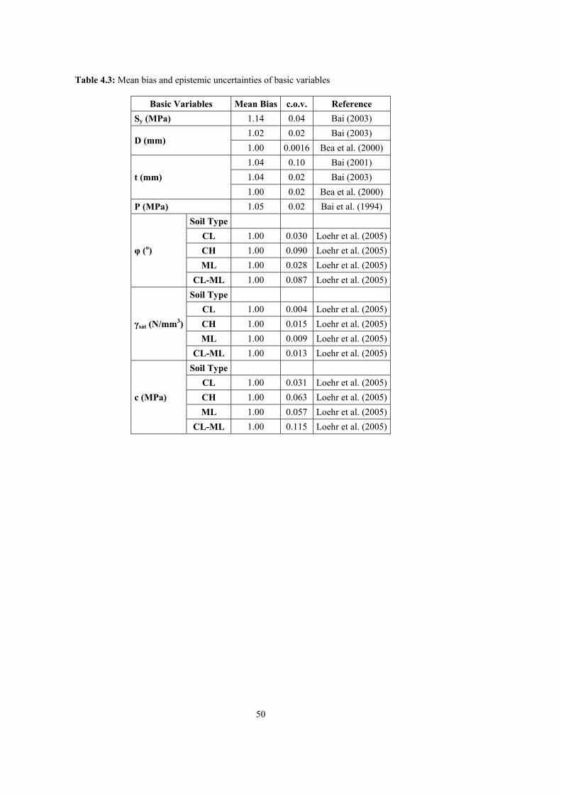
50

Table 4.3: Mean bias and epistemic uncertainties of basic variables

Basic Variables Mean Bias c.o.v. Reference

Sy (MPa) 1.14 0.04 Bai (2003)

D (mm) 1.02 0.02 Bai (2003)

1.00 0.0016 Bea et al. (2000)

t (mm)

1.04 0.10 Bai (2001)

1.04 0.02 Bai (2003)

1.00 0.02 Bea et al. (2000)

P (MPa) 1.05 0.02 Bai et al. (1994)

φ (o)

Soil Type

CL 1.00 0.030 Loehr et al. (2005)

CH 1.00 0.090 Loehr et al. (2005)

ML 1.00 0.028 Loehr et al. (2005)

CL-ML 1.00 0.087 Loehr et al. (2005)

γsat (N/mm3)

Soil Type

CL 1.00 0.004 Loehr et al. (2005)

CH 1.00 0.015 Loehr et al. (2005)

ML 1.00 0.009 Loehr et al. (2005)

CL-ML 1.00 0.013 Loehr et al. (2005)

c (MPa)

Soil Type

CL 1.00 0.031 Loehr et al. (2005)

CH 1.00 0.063 Loehr et al. (2005)

ML 1.00 0.057 Loehr et al. (2005)

CL-ML 1.00 0.115 Loehr et al. (2005)

51

4.5.1TensileFailure Buried continuous pipelines exhibit good performance under tensile loads on account of ductility. They can possess high tensile strains before rupture. However, ASCE (1984) states that “Stress concentrations due to weld discontinuities and nonuniformities in pipeline wall thickness, yield point, etc., could lead to pipeline failure at lower strain levels.” Therefore the strain at about rupture cannot be used as a limit state. ASCE (1984) recommends that “with good quality control to promote near uniformity of pipeline properties and weld inspection adequate to minimize weld flaws, maximum design tensile strain limits on the order of 2% to 5% be reasonable” based on the report of Kennedy et al. (1977). In this study 4% strain limit (εR) is adopted as the tensile resistance capacity based on the recommendations of O’Rourke et al. (1999).

4.5.2LocalBucklingFailure Buckling is the failure of the structure when it suddenly changes its situation from stable to unstable under compression loads. When the pipe wall locally loses its stability under compression, the state of “local buckling” or “wrinkling” occurs. The fact that the local buckling occurs does not mean that the failure of the pipeline will also occur at the same time. However, once the initial local buckling takes place, all load effects concentrate on that point and causes the pipeline failure in terms of circumferential cracking of the pipe wall. This is the most critical and most common failure mode of the pipeline. O’Rourke (2003) reported that “Wave propagation in the 1985 Michoacan (Mexico) event caused this type of damage for a water pipe in Mexico City, and PGD caused this type of damage to a liquid fuel pipeline in the 1991 Costa Rica event, and to water and gas pipelines in the 1994 Northridge event.” Compressive stresses may yield to such detrimental consequences for buried pipelines, therefore in the design of buried pipelines alternative options have to be taken into account as much as possible in order to avoid this type of failure. For example, when fault crossing is considered, the crossing angle is selected accordingly. The onset of wrinkling occurs at strains in the following range, based on prior laboratory tests on thin wall cylinders (Hall and Newmark, 1977): 0.15 0.20 4.39

where, t = wall thickness of pipe Rn = nominal radius of pipe Here the mean value of εcr as obtained from the lower and upper bounds of Equation 4.39 is used as the failure point and is taken as the local buckling resistance capacity, as follows: 0.175 4.40

where, εLb = local buckling strain capacity ri = inside radius of pipe

52

O’Rourke (2003) states that “this assumed wrinkling strain is thought to be appropriate for thin wall pipe but somewhat conservative for thicker wall pipe.” When buried continuous steel pipelines are considered, the wall thickness is generally thin and as O’Rourke (2003) stated, Equation 4.40 can be appropriately used for the local buckling capacity of those pipelines.

4.6DeterminationofLimitStateFunctions Limit state functions are determined corresponding to each earthquake effect described in Chapter 3 in addition to operating load effects described in Chapter 2. Operating loads, which are the loads due to internal pressure and temperature changes, are common for each limit state, and are presented below. As mentioned before, limit state functions are formed in terms of strains experienced by the pipeline. Accordingly, the limit state function given by Equation 4.1 takes the following form in this case: 4.41 where,

= 0.04 for tensile failure mode = 0.175 for local buckling failure mode

= for tensile failure mode = for local buckling failure mode

and are the tensile and compressive strains due to the corresponding earthquake effect,

respectively. Additionally, and are the tensile strains due to the internal pressure and temperature changes, respectively. The net compressive strain is taken into account, i.e. compressive strain is positively, tensile strain is negatively signed, for local buckling failure mode. In the estimation of the strains, the equations given in Chapters 2 and 3 are utilized. Since internal radius (ri) is generally used in the calculations of the load due to internal pressure, ri is inserted into these equations instead of diameter (D). Moreover, soil induced forces (tu, Pu, see Appendix A) and material properties (area, section modulus) are explicitly substituted into corresponding equations. These modified equations, utilized in estimating tensile and compressive strains, are listed in Table 4.4. Furthermore, tensile strains due to internal pressure and temperature changes are given as follows: 1 1 4.42

∆ 1 1 ∆ 4.43

where, P = internal pressure ν = Poisson’s ratio E = steel modulus of elasticity Sy = yield strength of the pipe material

53

Table 4.4: Tensile ( ) and compressive ( ) strain equations corresponding to each earthquake effect and the related method

Earthquake Effect

Case or Method

Direction Corresponding Strain

Equation

Seismic Wave Propagation

1 tensile and

compressive

2 tensile and

compressive

Lateral Spreading (Longitudinal

PGD)

1 tensile and

compressive 1

2 tensile and

compressive 1

Lateral Spreading (Transverse

PGD)

1 tensile and

compressive

2 tensile and

compressive′

Buoyancy

1 tensile and

compressive 1

2

tensile

compressive

Fault Crossing

Newmark Hall (1975)

tensile 2

Kennedy et al. (1977)

tensile 1

Notes: i) 2 ′ 2 sin ′ tan ′

ii)

iii) For the definition of the symbols used to denote the basic variables and strains, please refer to the previous sections and Appendix A or “List of Symbols and Abbreviations” section.

54

n, r = Ramberg-Osgood parameters (see Table 2.1) αt = linear coefficient of thermal expansion of steel ΔT = temperature change For seismic wave propagation, longitudinal PGD, transverse PGD and liquefaction induced buoyancy effects, there are two cases to be considered as mentioned in Chapter 3. For each of these earthquake effects and the resulting failure modes, as indicated earlier, the case which provides the smaller strain is to be used, and the corresponding limit state function is to be formed by utilizing Equation 4.41 and Table 4.4. For fault crossing effects, Newmark Hall (1975) and Kennedy et al. (1977) methods are considered and these methods are applicable only to pipes under tensile forces. Limit state functions corresponding to tensile failure due to fault crossing effects according to these two methods are to be formed by utilizing Equation 4.41 and Table 4.4.

4.7CalculationofSurvivalProbability In order to perform the reliability analysis and calculate the probability of survival or failure, first the basic random variables are determined. In this thesis, all random variables are assumed to be normally distributed and their mean and variance values are obtained from the sources cited in Section 4.4 and Chapter 5. In order to estimate the reliability indexes and the corresponding survival probabilities, Advanced First Order Second Moment Method is used. All the calculations are performed by using the relevant computer programs, Mathcad and MS Excel. Reliability indexes, βHL, are estimated for all limit states defined in Section 4.6. From these βHL values survival probabilities are obtained by using the standard normal distribution table. For fault crossing, survival probabilities calculated from Newmark Hall (1975) and Kennedy et al. (1977) methods are assumed to be equally likely and therefore the survival probability of a fault crossing is taken as the average of those computed from these two methods. Two case studies are presented in the next chapter in order to show the implementation of the methodology and concepts presented up to here.

55

CHAPTER5

CASESTUDIES

5.1Introduction In this chapter, two case studies are carried out. For the first case study, only the load due to internal pressure is considered. For the second one, in addition to the load due to internal pressure, load due to temperature changes and loads due to earthquake induced effects are taken into consideration. In these case studies, two existing natural gas pipelines are examined. For the first case study, 16” (16 inches) Hatay Natural Gas Pipeline, where the aim is to convey natural gas to Antakya city and its districts, is considered. For the second case study, 36” (36 inches) Turkey-Greece Natural Gas Pipeline, which transports the Caspian natural gas to Europe, is examined.

5.2CaseStudy1:LoadduetoInternalPressure As discussed in Chapter 2, buried steel pipelines are primarily subjected to load due to internal pressure when they are under operation. In order to sustain their functions properly, they should be designed in such a way that the desired reliability is attained. Let a section of a pipeline having a uniform diameter and grade be considered. Once the diameter of the pipeline is determined from hydraulic analysis, then the key element to resist the load due to internal pressure will be the pipe wall thickness. For a natural gas pipeline under high pressure, Equation 2.1, taken from ASME B31.8 code (2010), is used to evaluate the wall thickness deterministically. If Equation 2.1 is revised with respect to wall thickness, t, Equation 2.1 becomes: 2 1 5.1

where, P = design pressure D = nominal outside diameter of pipe Sy = yield strength t = nominal wall thickness F = design (safety) factor E = longitudinal joint factor T = temperature derating factor

Moreovpopulatin EquaobserveTable 5 Table 5

For thebe seenparts olength, approxof 16 in

Figurecolor

ver, in ASMEtion density ination 5.1, is deed in Table 55.1 since it is n

5.1: Safety fac

e first case stun from Figureof different di

whereas the simately 137 knches, and hav

e 5.1: Hatay N

E B31.8 coden the proximiecreased with

5.1. For Locatnot considered

ctors to be use

Lo1,

udy, the reliabe 5.1, Hatay Piameters. Thesecond branchkm. In this stuving material

Natural Gas Pip

e (2010), fouity of the pipe increased poption Class 1, d in this study

ed in design (C

cation Class, Division 2

2 3 4

ility of the Haipeline branch

e first branch h is 16” in diady, only the sgrade of API

peline. The po

56

ur location claeline to be conpulation and cthere is also

y.

Cited from AS

Safety Fact0.720.600.500.40

atay Natural Ghes off from 4is 36” in dia

ameter and lonecond branch5L X52 is con

ortion of the p

asses are idennstructed. ThecorrespondingDivision 1 w

SME B31.8, 2

tor (F)

Gas Pipeline i40” main pipeameter and a

nger than the f which has a nnsidered (BOT

pipeline exami

ntified accorde design safet

g location claswhich is not i

2010)

is to be assesseline and split

approximately first one with nominal pipe TAŞ, 2009).

ined is marke

ding to the ty factor, F s as can be ncluded in

sed. As can ts into two 20 km in

a length of size (NPS)

d in purple

57

The steel pipe is manufactured with submerged arc welding process by longitudinal seam. The design temperature interval is in between -5oC and 50oC and the design pressure is 75 bars. There is no corrosion allowance and the nominal values of the basic variables are given in Table 5.2 (BOTAŞ, 2009). Table 5.2: Nominal values of basic variables (Cited from BOTAŞ, 2009)

Basic Variable Nominal Value

D (mm) 406.4

P (MPa) 7.5

Sy (Mpa) 359

Temperature (oC) 15

E(i) 1

T(ii) 1 Notes:

i) Longitudinal joint factor, E, is taken as 1 for longitudinally submerged arc welded pipe from Table 841.1.7-1 of ASME B 31.8 (2010)

ii) Temperature derating factor, T, is taken as 1 for design temperature less than 121oC from Table 841.1.8-1 of ASME B 31.8 (2010)

Using Equation 5.1, nominal wall thicknesses are calculated deterministically for each location classes as indicated in Table 5.3. In that table, both computed values of wall thicknesses from Equation 5.1 and nominal values of wall thicknesses, which correspond to the nearest nominal thickness above the computed thickness in the pipe mill catalog and also correspond to the values in BOTAŞ (2009) specifications, are shown. Additionally, nominal internal radii corresponding to the nominal wall thicknesses are given in this table. Table 5.3: Values of nominal wall thicknesses and internal radii as taken from BOTAŞ (2009) specifications and computed wall thicknesses for location classes for NPS 16 steel pipeline

Location Class tnominal (mm) ri-nominal (mm) tcomputed (mm)

1, Division 2 6.4 196.8 5.896

2 7.1 196.1 7.075

3 8.7 194.5 8.490

4 11.1 192.1 10.613 In order to carry out the reliability calculations, basic variables are identified and are listed in Table 5.4 together with their statistical parameters. In this table, mean biases (N), average values (X), calculated mean values (µ), coefficients of variation for quantifying aleatory (δ) and epistemic (Δ) uncertainties and calculated total uncertainties (Ω) of the basic variables are listed. In the determination of these values, data collected from Hatay Pipeline Project (BOTAŞ, 2009), Table 4.2 and Table 4.3 are utilized. All these random variables are assumed to be normally distributed and statistically independent.

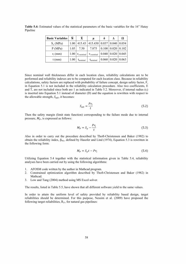
58

Table 5.4: Estimated values of the statistical parameters of the basic variables for the 16” Hatay Pipeline

Basic Variables µ δ Δ Ω

Sy (MPa) 1.00 415.43 415.430 0.037 0.040 0.054

P (MPa) 1.05 7.50 7.875 0.100 0.020 0.102

ri (mm) 1.00 ri-nominal ri-nominal 0.040 0.020 0.045

t (mm) 1.00 tnominal tnominal 0.060 0.020 0.063

Since nominal wall thicknesses differ in each location class, reliability calculations are to be performed and reliability indexes are to be computed for each location class. Because in reliability calculations, safety factors are replaced with probability of failure concept, design safety factor, F, in Equation 5.1 is not included in the reliability calculation procedure. Also two coefficients, E and T, are not included since both are 1 as indicated in Table 5.2. Moreover, if internal radius (ri) is inserted into Equation 5.1 instead of diameter (D) and the equation is rewritten with respect to the allowable strength, , it becomes: 5.2

Then the safety margin (limit state function) corresponding to the failure mode due to internal pressure, , is expressed as follows: 5.3

Also in order to carry out the procedure described by Thoft-Christensen and Baker (1982) to obtain the reliability index, βHL, defined by Hasofer and Lind (1974), Equation 5.3 is rewritten in the following form: 5.4 Utilizing Equation 5.4 together with the statistical information given in Table 5.4, reliability analyses have been carried out by using the following algorithms: 1. AFOSM code written by the author in Mathcad program. 2. Constrained optimization algorithm described by Thoft-Christensen and Baker (1982) in

Mathcad. 3. Low and Tang (2004) method using MS Excel solver. The results, listed in Table 5.5, have shown that all different software yield to the same values. In order to attain the uniform level of safety provided by reliability based design, target reliabilities should be determined. For this purpose, Nessim et al. (2009) have proposed the following target reliabilities, R , for natural gas pipelines:

59

Table 5.5: Reliability indexes calculated based on different computer software corresponding to different location class and mean wall thickness combinations

Location Class

μt (mm) Reliability Index (βHL)

Mathcad Code

Constrained Optimization

Excel Solver

1 6.4 4.025290 4.025288 4.025288

2 7.1 4.834288 4.834288 4.834288

3 8.7 6.403260 6.403261 6.403261

4 11.1 8.225847 8.225844 8.225844

R1 72PD . ρ 0 1 9ρPD . 0.0 D 1.0 x 10 1 450ρPD 1.0x10 D 6.0 x 10 1 2.1 x 10ρPD . ρPD 6.0 10

5.5

where, R = target reliability ρ = people per hectare P = pressure in psi D = diameter in inches People per hectare, ρ, values are also provided for each location class by Nessim et al. (2009) and are listed in Table 5.6. For the example considered, target reliabilities and reliability indexes are calculated from Equation 5.5, and the results are given in Table 5.6. Table 5.6: Target reliability indexes for different location classes for the Hatay pipeline as obtained from Equation 5.5

Location Class 1 2 3 4

ρ (people per hectare) 0.04 3.3 18 100

P (bar) 75 75 75 75

D (inch) 16 16 16 16

ρ*P*D3 1.78E+05 1.47E+07 8.02E+07 4.46E+08

Target Reliability (RT) 0.9974755 0.9999694 0.9999953 0.9999997

Target Reliability Index (βT) 2.803835 4.008095 4.428825 4.988168 The reliability analysis is repeated in order to achieve the target reliability indexes given in Table 5.6. For this purpose, wall thickness, t, values are modified to attain the target reliability indexes. Again, the three algorithms, mentioned above, are used to perform the reliability computations. Table 5.7 summarizes the resulting values.

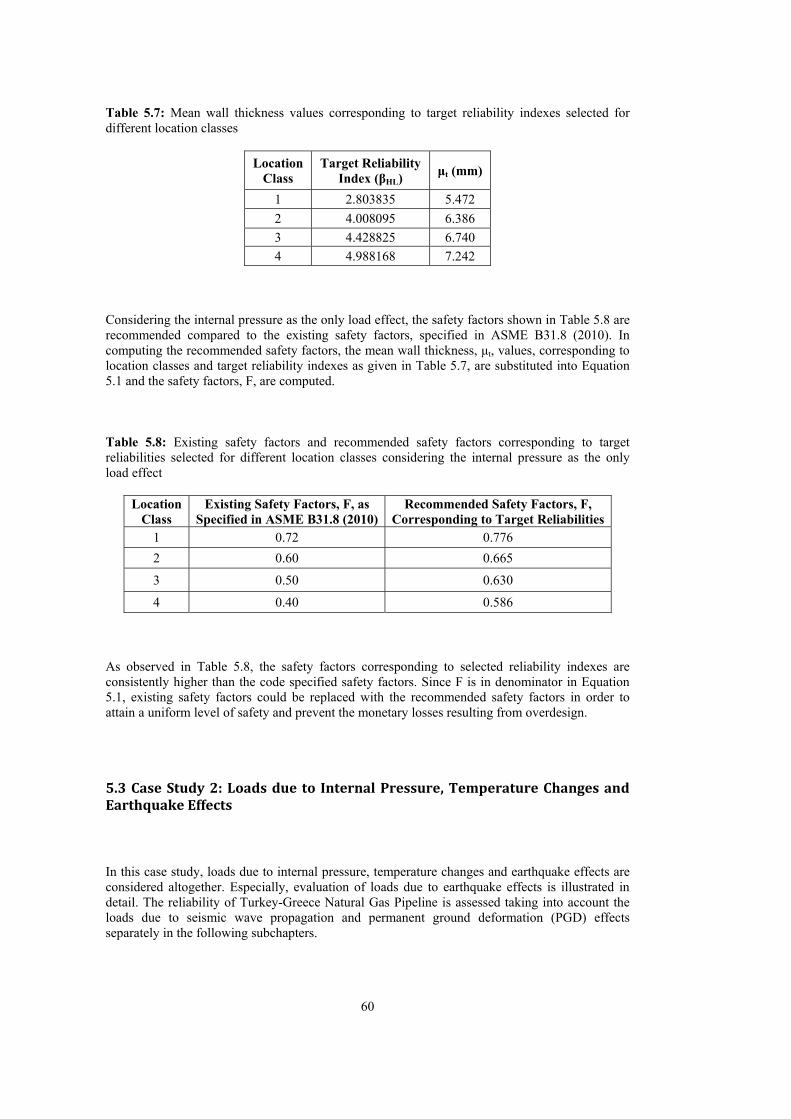
60

Table 5.7: Mean wall thickness values corresponding to target reliability indexes selected for different location classes

Location Class

Target Reliability Index (βHL)

μt (mm)

1 2.803835 5.472

2 4.008095 6.386

3 4.428825 6.740

4 4.988168 7.242 Considering the internal pressure as the only load effect, the safety factors shown in Table 5.8 are recommended compared to the existing safety factors, specified in ASME B31.8 (2010). In computing the recommended safety factors, the mean wall thickness, μt, values, corresponding to location classes and target reliability indexes as given in Table 5.7, are substituted into Equation 5.1 and the safety factors, F, are computed. Table 5.8: Existing safety factors and recommended safety factors corresponding to target reliabilities selected for different location classes considering the internal pressure as the only load effect

Location Class

Existing Safety Factors, F, as Specified in ASME B31.8 (2010)

Recommended Safety Factors, F, Corresponding to Target Reliabilities

1 0.72 0.776

2 0.60 0.665

3 0.50 0.630

4 0.40 0.586 As observed in Table 5.8, the safety factors corresponding to selected reliability indexes are consistently higher than the code specified safety factors. Since F is in denominator in Equation 5.1, existing safety factors could be replaced with the recommended safety factors in order to attain a uniform level of safety and prevent the monetary losses resulting from overdesign.

5.3CaseStudy2:Loadsdue to InternalPressure,TemperatureChangesandEarthquakeEffects In this case study, loads due to internal pressure, temperature changes and earthquake effects are considered altogether. Especially, evaluation of loads due to earthquake effects is illustrated in detail. The reliability of Turkey-Greece Natural Gas Pipeline is assessed taking into account the loads due to seismic wave propagation and permanent ground deformation (PGD) effects separately in the following subchapters.

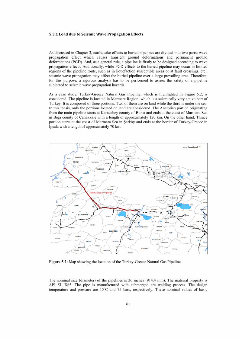
61

5.3.1LoadduetoSeismicWavePropagationEffects As discussed in Chapter 3, earthquake effects to buried pipelines are divided into two parts: wave propagation effect which causes transient ground deformations and permanent ground deformations (PGD). And, as a general rule, a pipeline is firstly to be designed according to wave propagation effects. Additionally, while PGD effects to the buried pipeline may occur in limited regions of the pipeline route, such as in liquefaction susceptible areas or at fault crossings, etc., seismic wave propagation may affect the buried pipeline over a large prevailing area. Therefore, for this purpose, a rigorous analysis has to be performed to assess the safety of a pipeline subjected to seismic wave propagation hazards. As a case study, Turkey-Greece Natural Gas Pipeline, which is highlighted in Figure 5.2, is considered. The pipeline is located in Marmara Region, which is a seismically very active part of Turkey. It is composed of three portions. Two of them are on land while the third is under the sea. In this thesis, only the portions located on land are considered. The Anatolian portion originating from the main pipeline starts at Karacabey county of Bursa and ends at the coast of Marmara Sea in Biga county of Çanakkale with a length of approximately 120 km. On the other hand, Thrace portion starts at the coast of Marmara Sea in Şarköy and ends at the border of Turkey-Greece in İpsala with a length of approximately 70 km.

Figure 5.2: Map showing the location of the Turkey-Greece Natural Gas Pipeline The nominal size (diameter) of the pipelines is 36 inches (914.4 mm). The material property is API 5L X65. The pipe is manufactured with submerged arc welding process. The design temperature and pressure are 15oC and 75 bars, respectively. These nominal values of basic

variabllayers o Table 5

The MintersectransitiPipelinCaspianintegritactive iearthqu

FigureŞaroğlu

es are tabulatof polyethylen

5.9: Nominal

armara regionction point oon area betw

ne connecting n gas to Euroty. Since Marin terms of seuake occurs, th

e 5.3: Main fau et al., 1992)

ted in Table 5ne.

values of basi

B

Te

n, the most poof the contineween these co

the Turkish popean customrmara region eismicity, the phe pipeline sh

aults in the vi

5.9. Also for c

ic variables fo

Basic Variabl

D (mm) t (mm)

P (MPa) Sy (MPa)

emperature (oCE T

opulated and entals, Europeontinentals. Tpipeline netw

mers. Not to iaccommodatipipeline has t

hould sustain it

icinity of Tur

62

corrosion pro

or Turkey-Gre

e Nominal V

914.411.97.5448

C) 1511

industrializede and Asia.

This is also twork with Eur

nterrupt this ing the portioto be earthquats function an

rkey-Greece N

tection, the p

eece Natural G

Value

4 9

d region of TuThat is why rue for Turkropean pipelinflow, the pip

on of the pipake resistant. Ind be sufficien

Natural Gas P

pipeline is coa

Gas Pipeline

urkey, is situit has the p

key-Greece Nnes so as to cpeline should eline in TurkIn other wordntly reliable.

Pipeline (Mod

ated with 3

ated at the property of atural Gas convey the sustain its

key is very ds, when an

dified from

63

Figure 5.4: Seismicity of Marmara region (Cited from Kalkan et al., 2009) Table 5.10: Earthquakes with M ≥ 6.0 recorded in the Marmara region during the years 1905-1999 (Cited from Kalkan et al., 2009)

No Year Month Day Latitude Long. M 1 1905 4 15 40.20 29.00 6.6 2 1912 8 10 40.60 27.20 7.4 3 1919 11 18 39.20 27.40 7.0 4 1928 5 3 39.64 29.14 6.1 5 1935 1 4 40.40 27.49 6.7 6 1939 9 22 39.07 29.94 7.1 7 1939 10 19 39.07 26.94 6.6 8 1942 6 16 40.80 27.80 6.0 9 1943 6 20 40.85 30.51 6.6

10 1944 6 25 39.05 29.26 6.1 11 1944 10 6 39.48 26.56 7.0 12 1953 3 18 39.99 27.36 6.6 13 1956 2 20 39.89 30.49 6.4 14 1957 5 26 40.67 31.00 6.7 15 1961 11 28 40.00 26.30 6.0 16 1964 10 6 40.30 28.23 6.9 17 1966 8 21 40.33 27.40 6.0 18 1967 7 22 40.70 30.70 6.7 19 1970 3 28 39.21 29.51 7.1 20 1971 5 25 39.03 29.74 6.1 21 1975 3 27 40.42 26.14 6.7 22 1976 8 25 39.30 28.80 6.0 23 1976 9 6 39.06 29.00 6.6 24 1999 8 17 40.76 29.97 7.4 25 1999 11 12 40.74 31.21 7.2

64

Main faults in the vicinity of the pipeline are illustrated in Figure 5.3. Also on this figure, the route of the pipeline with respect to the faults can be seen. Besides these faults, seismicity of the region is displayed by plotting the epicenters of the major earthquakes whose moment magnitudes (M) are greater than 4 in Figure 5.4. Also in Table 5.10, those earthquakes having M greater than 6 are listed. For the last century it has been observed that 25 earthquakes have occurred and 7 of them were major seismic events having magnitudes of 7 or above. In order to evaluate the reliability of the pipeline subject to seismic wave propagation effects, peak ground velocities (PGV) along the pipeline route should be obtained. For this purpose, in the design phase, probabilistic seismic hazard maps providing acceleration and velocity levels at National Earthquake Hazards Reduction Program (NEHRP) B site class for earthquakes having 10% and 2% probabilities of exceedance in 50 years, corresponding to return periods of about 475 and 2475 years, respectively, were prepared for the pipeline route (BOTAŞ, 2003).

Figure 5.5: PGV contour map at NEHRP B site class for 10% probability of exceedance in 50 years (Cited from BOTAŞ, 2003) In the preparation of these probabilistic seismic hazard maps, two different levels of ground motion are considered. These are Functional Evaluation Earthquake ground motion (FEE) and Safety Evaluation Earthquake ground motion (SEE). The first level of ground motion, FEE, corresponds to earthquakes that can reasonably affect the pipeline at any location during its lifetime and that have 10% probability of exceedence during an economic lifetime of 50 years, similar to the Turkish Seismic Code for Buildings (TSC, 2007). Additionally, the pipeline should

65

be fully operational in case an earthquake in this level occurs. On the other hand, the second level of ground motion, SEE, corresponds to earthquakes having 2% probability of exceedence during an economic lifetime of 50 years. Besides, only repairable damage is allowed in case the pipeline is subjected to this level of ground motion. Nevertheless, in this situation, the pipeline may be deformed but should not leak (BOTAŞ, 2003). Peak ground velocity contour maps at NEHRP B site class for earthquakes having 10% and 2% probabilities of exceedance in 50 years, which conforms to FEE and SEE levels of ground motions, are given as cited from BOTAŞ (2003) in Figures 5.5 and 5.6, respectively.

Figure 5.6: PGV contour map at NEHRP B site class for 2% probability of exceedance in 50 years (Cited from BOTAŞ, 2003) These PGV values for NEHRP site class B obtained from contour maps (see Table B.1 in Appendix B for classification of site) can be utilized in order to find the local PGV values corresponding to own specific site class in the pipeline route by using the equation below (ALA, 2005 as modified from NEHRP, 1997): 5.6 where,

= local design peak ground velocity

66

= peak ground velocity at site class B = site coefficient (see Table 5.11)

Table 5.11: Site coefficient, Fv, as a function of site class and PGVB (Cited from ALA, 2005 as modified from NEHRP, 1997)

Site Class

Alignment Specific PGV for Rock (Site Class B) PGVB ≤ 100

mm/s PGVB = 200

mm/s PGVB = 300

mm/s PGVB = 400

mm/s PGVB ≥ 500

mm/s A 0.8 0.8 0.8 0.8 0.8 B 1.0 1.0 1.0 1.0 1.0 C 1.7 1.6 1.5 1.4 1.3 D 2.4 2.0 1.8 1.6 1.5 E 3.5 3.2 2.8 2.4 2.4 F * * * * *

Note: Site-specific geotechnical investigation and dynamic site response analyses are

recommended to develop appropriate values. From Figures 5.5 and 5.6, mean peak ground velocities corresponding to earthquakes having 10% (PGVB-0.10) and 2% (PGVB-0.02) probabilities of exceedance in 50 years, at site class B were obtained and these values were amplified by using Equation 5.6 in order to compute local design peak ground velocities corresponding to earthquakes having 10% (PGV0.10) and 2% (PGV0.02) probabilities of exceedance in 50 years, at specified site classes in the pipeline route as given in Table 5.12. It is seen in this table that the whole pipeline is examined in 66 segments, which are denoted with numbers in this and following tables, in accordance with the geotechnical investigations. The format of this segmentation and corresponding site classes are obtained from BOTAŞ (2003). In order to carry out reliability calculations, basic variables defined with their statistical parameters in Table 5.13 are to be used. In this table, mean biases, average values, calculated mean values, coefficients of variation for quantifying aleatory and epistemic uncertainties and calculated total uncertainties of the basic variables are listed. In the determination of these values, Table 4.2 and Table 4.3 are utilized. The total length of the route is assumed as “location class 1” according to ASME B31.8 (2010) and therefore wall thickness is taken to be constant. Throughout the route of the pipeline shear wave velocity is assumed to be dominant over Rayleigh wave. Mean values of shear wave velocities are assumed to be the average values given for each site class in Table B.1. Moreover, uncertainties of PGV, shear wave velocity and wavelength are assumed as given in Table 5.13. All the basic random variables involved are assumed to be normally distributed and statistically independent. Along the route of the pipeline, three different site classes according to NEHRP (1997) are observed and four soil types, according to unified soil classification system (see Appendix B, Table B.2), in which the pipeline is buried are dominant (BOTAŞ, 2003). These site classes and soil types can be seen in Tables 5.12, 5.13 and 5.14. As discussed in Chapter 3, to perform reliability calculations, mean values of axial strain (εa) due to wave propagation and maximum strain (εmax) due to soil friction have to be evaluated by using Equations 3.1 and 3.2, respectively. Then they should be compared and the lower value should be selected as the seismic strain (εwp) to be used in further calculations.

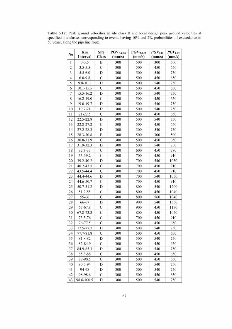
67

Table 5.12: Peak ground velocities at site class B and local design peak ground velocities at specified site classes corresponding to events having 10% and 2% probabilities of exceedance in 50 years, along the pipeline route

No Km

Interval Site

ClassPGVB-0.10

(mm/s) PGVB-0.02

(mm/s) PGV0.10

(mm/s) PGV0.02

(mm/s)

1 0-3.5 B 300 500 300 500 2 3.5-5.5 C 300 500 450 650 3 5.5-6.0 D 300 500 540 750 4 6.0-9.8 C 300 500 450 650 5 9.8-10.1 D 300 500 540 750 6 10.1-15.5 C 300 500 450 650 7 15.5-16.2 D 300 500 540 750 8 16.2-19.0 C 300 500 450 650 9 19.0-19.7 D 300 500 540 750

10 19.7-21 D 300 500 540 750 11 21-22.5 C 300 500 450 650 12 22.5-22.8 D 300 500 540 750 13 22.8-27.2 C 300 500 450 650 14 27.2-28.3 D 300 500 540 750 15 28.3-30.8 B 300 500 300 500 16 30.8-31.9 C 300 500 450 650 17 31.9-32.3 D 300 500 540 750 18 32.3-33 C 300 600 450 780 19 33-39.2 C 300 700 450 910 20 39.2-40.2 D 300 700 540 1050 21 40.2-43.5 C 300 700 450 910 22 43.5-44.4 C 300 700 450 910 23 44.4-44.6 D 300 700 540 1050 24 44.6-50.7 C 300 700 450 910 25 50.7-51.2 D 300 800 540 1200 26 51.2-55 C 300 800 450 1040 27 55-66 C 400 800 560 1040 28 66-67 D 300 900 540 1350 29 67-67.8 C 300 900 450 1170 30 67.8-73.3 C 300 800 450 1040 31 73.3-76 C 300 700 450 910 32 76-77.5 C 300 500 450 650 33 77.5-77.7 D 300 500 540 750 34 77.7-81.8 C 300 500 450 650 35 81.8-82 D 300 500 540 750 36 82-84.9 C 300 500 450 650 37 84.9-85.3 D 300 500 540 750 38 85.3-88 C 300 500 450 650 39 88-90.5 C 300 500 450 650 40 90.5-94 D 300 500 540 750 41 94-98 D 300 500 540 750 42 98-98.6 C 300 500 450 650 43 98.6-100.5 D 300 500 540 750

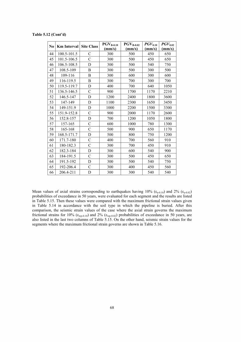
68


No Km Interval Site Class PGVB-0.10

(mm/s) PGVB-0.02

(mm/s) PGV0.10

(mm/s) PGV0.02

(mm/s) 44 100.5-101.5 C 300 500 450 650 45 101.5-106.5 C 300 500 450 650 46 106.5-108.5 D 300 500 540 750 47 108.5-109 B 300 500 300 500 48 109-116 B 300 600 300 600 49 116-119.5 B 300 700 300 700 50 119.5-119.7 D 400 700 640 1050 51 136.5-146.5 C 900 1700 1170 2210 52 146.5-147 D 1200 2400 1800 3600 53 147-149 D 1100 2300 1650 3450 54 149-151.9 D 1000 2200 1500 3300 55 151.9-152.8 C 900 2000 1170 2600 56 152.8-157 D 700 1200 1050 1800 57 157-165 C 600 1000 780 1300 58 165-168 C 500 900 650 1170 59 168.5-171.7 D 500 800 750 1200 60 171.7-180 C 400 700 560 910 61 180-182.3 C 300 700 450 910 62 182.3-184 D 300 600 540 900 63 184-191.5 C 300 500 450 650 64 191.5-192 D 300 500 540 750 65 192-206.4 C 300 400 450 560 66 206.4-211 D 300 300 540 540

Mean values of axial strains corresponding to earthquakes having 10% (εa-0.10) and 2% (εa-0.02) probabilities of exceedance in 50 years, were evaluated for each segment and the results are listed in Table 5.15. Then these values were compared with the maximum frictional strain values given in Table 5.14 in accordance with the soil type in which the pipeline is buried. After this comparison, the seismic strain values of the case where the axial strain governs the maximum frictional strains for 10% (εwp-0.10) and 2% (εwp-0.02) probabilities of exceedance in 50 years, are also listed in the last two columns of Table 5.15. On the other hand, seismic strain values for the segments where the maximum frictional strain governs are shown in Table 5.16.

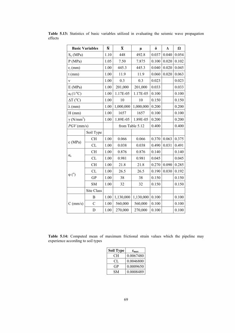
69

Table 5.13: Statistics of basic variables utilized in evaluating the seismic wave propagation effects


Sy (MPa) 1.10 448 492.8 0.037 0.040 0.054

P (MPa) 1.05 7.50 7.875 0.100 0.020 0.102

ri (mm) 1.00 445.3 445.3 0.040 0.020 0.045

t (mm) 1.00 11.9 11.9 0.060 0.020 0.063

ν 1.00 0.3 0.3 0.023 0.023

E (MPa) 1.00 201,000 201,000 0.033 0.033

αt (1/oC) 1.00 1.17E-05 1.17E-05 0.100 0.100

ΔT (oC) 1.00 10 10 0.150 0.150

λ (mm) 1.00 1,000,000 1,000,000 0.200 0.200

H (mm) 1.00 1657 1657 0.100 0.100

γ (N/mm3) 1.00 1.89E-05 1.89E-05 0.200 0.200

PGV (mm/s) from Table 5.12 0.400 0.400

Soil Type

c (MPa) CH 1.00 0.066 0.066 0.370 0.063 0.375

CL 1.00 0.038 0.038 0.490 0.031 0.491

αc CH 1.00 0.876 0.876 0.140 0.140

CL 1.00 0.981 0.981 0.045 0.045

φ (o)

CH 1.00 21.8 21.8 0.270 0.090 0.285

CL 1.00 26.5 26.5 0.190 0.030 0.192

GP 1.00 38 38 0.150 0.150

SM 1.00 32 32 0.150 0.150

Site Class

C (mm/s)

B 1.00 1,130,000 1,130,000 0.100 0.100

C 1.00 560,000 560,000 0.100 0.100

D 1.00 270,000 270,000 0.100 0.100

Table 5.14: Computed mean of maximum frictional strain values which the pipeline may experience according to soil types

Soil Type εmax CH 0.0067480CL 0.0046800GP 0.0009650SM 0.0008489

70

Table 5.15: Mean values of local design peak ground and seismic wave propagation velocities, axial strains and governing axial strains for events having 10% and 2% probabilities of exceedance in 50 years

No Site

Class PGV0.10

(mm/s) PGV0.02

(mm/s) C

(mm/s) εa-0.10 εa-0.02 εwp-0.10 εwp-0.02

1 B 300 500 1130000 0.00013 0.00022 0.00013 0.00022 2 C 450 650 560000 0.00040 0.00058 0.00040 0.00058 3 D 540 750 270000 0.00100 0.00139 not not 4 C 450 650 560000 0.00040 0.00058 0.00040 0.00058 5 D 540 750 270000 0.00100 0.00139 not not 6 C 450 650 560000 0.00040 0.00058 0.00040 0.00058 7 D 540 750 270000 0.00100 0.00139 0.00100 0.00139 8 C 450 650 560000 0.00040 0.00058 0.00040 0.00058 9 D 540 750 270000 0.00100 0.00139 not not

10 D 540 750 270000 0.00100 0.00139 not not 11 C 450 650 560000 0.00040 0.00058 0.00040 0.00058 12 D 540 750 270000 0.00100 0.00139 not not 13 C 450 650 560000 0.00040 0.00058 0.00040 0.00058 14 D 540 750 270000 0.00100 0.00139 not not 15 B 300 500 1130000 0.00013 0.00022 0.00013 0.00022 16 C 450 650 560000 0.00040 0.00058 0.00040 0.00058 17 D 540 750 270000 0.00100 0.00139 not not 18 C 450 780 560000 0.00040 0.00070 0.00040 0.00070 19 C 450 910 560000 0.00040 0.00081 0.00040 0.00081 20 D 540 1050 270000 0.00100 0.00194 0.00100 0.00194 21 C 450 910 560000 0.00040 0.00081 0.00040 0.00081 22 C 450 910 560000 0.00040 0.00081 0.00040 0.00081 23 D 540 1050 270000 0.00100 0.00194 0.00100 0.00194 24 C 450 910 560000 0.00040 0.00081 0.00040 0.00081 25 D 540 1200 270000 0.00100 0.00222 not not 26 C 450 1040 560000 0.00040 0.00093 0.00040 0.00093 27 C 560 1040 560000 0.00050 0.00093 0.00050 not 28 D 540 1350 270000 0.00100 0.00250 not not 29 C 450 1170 560000 0.00040 0.00104 0.00040 not 30 C 450 1040 560000 0.00040 0.00093 0.00040 not 31 C 450 910 560000 0.00040 0.00081 0.00040 0.00081 32 C 450 650 560000 0.00040 0.00058 0.00040 0.00058 33 D 540 750 270000 0.00100 0.00139 not not 34 C 450 650 560000 0.00040 0.00058 0.00040 0.00058 35 D 540 750 270000 0.00100 0.00139 0.00100 0.00139 36 C 450 650 560000 0.00040 0.00058 0.00040 0.00058 37 D 540 750 270000 0.00100 0.00139 not not 38 C 450 650 560000 0.00040 0.00058 0.00040 0.00058 39 C 450 650 560000 0.00040 0.00058 0.00040 0.00058 40 D 540 750 270000 0.00100 0.00139 not not 41 D 540 750 270000 0.00100 0.00139 not not 42 C 450 650 560000 0.00040 0.00058 0.00040 0.00058 43 D 540 750 270000 0.00100 0.00139 not not

71


No Site

Class PGV0.10

(mm/s) PGV0.02

(mm/s) C

(mm/s) εa-0.10 εa-0.02 εwp-0.10 εwp-0.02

44 C 450 650 560000 0.00040 0.00058 0.00040 0.00058 45 C 450 650 560000 0.00040 0.00058 0.00040 0.00058 46 D 540 750 270000 0.00100 0.00139 not not 47 B 300 500 1130000 0.00013 0.00022 0.00013 0.00022 48 B 300 600 1130000 0.00013 0.00027 0.00013 0.00027 49 B 300 700 1130000 0.00013 0.00031 0.00013 0.00031 50 D 640 1050 270000 0.00119 0.00194 not not 51 C 1170 2210 560000 0.00104 0.00197 not not 52 D 1800 3600 270000 0.00333 0.00667 not not 53 D 1650 3450 270000 0.00306 0.00639 not not 54 D 1500 3300 270000 0.00278 0.00611 not not 55 C 1170 2600 560000 0.00104 0.00232 not not 56 D 1050 1800 270000 0.00194 0.00333 not not 57 C 780 1300 560000 0.00070 0.00116 not not 58 C 650 1170 560000 0.00058 0.00104 not not 59 D 750 1200 270000 0.00139 0.00222 not not 60 C 560 910 560000 0.00050 0.00081 0.00050 0.00081 61 C 450 910 560000 0.00040 0.00081 0.00040 0.00081 62 D 540 900 270000 0.00100 0.00167 not not 63 C 450 650 560000 0.00040 0.00058 0.00040 0.00058 64 D 540 750 270000 0.00100 0.00139 not not 65 C 450 560 560000 0.00040 0.00050 0.00040 0.00050 66 D 540 540 270000 0.00100 0.00100 not not

Notes: i) “not” denotes the case where the axial strain does not govern.

ii) For segments 7, 20 and 23, soil types are CH; for segment 26, two soil types, which are CH and GP, are common; for segment 35, soil type is CL.

Table 5.16: Mean axial strain and the mean strain values for the segments where maximum frictional strain governs for events having 10% and 2% probabilities of exceedance in 50 years

No Site Class Soil Type εa-0.10 εa-0.02 εwp-0.10 εwp-0.02

3 D SM 0.00100 0.00139 0.00085 0.00085 5 D SM 0.00100 0.00139 0.00085 0.00085 9 D SM 0.00100 0.00139 0.00085 0.00085

10 D SM 0.00100 0.00139 0.00085 0.00085 28 D SM 0.00100 0.00250 0.00085 0.00085 33 D SM 0.00100 0.00139 0.00085 0.00085 43 D SM 0.00100 0.00139 0.00085 0.00085 50 D GP 0.00119 0.00194 0.00097 0.00097 52 D SM 0.00333 0.00667 0.00085 0.00085 55 C SM 0.00104 0.00232 0.00085 0.00085 56 D SM 0.00194 0.00333 0.00085 0.00085 57 C SM 0.00070 0.00116 εa governs 0.00085 66 D SM 0.00100 0.00100 0.00085 0.00085

72

Moreover, in some segments of the pipeline route, there are more than one major soil type in which the pipeline is buried. For these segments, which are listed in Table 5.17, maximum frictional strains were computed for the soil types giving the highest (denoted in Table 5.17 as 1) and the lowest (denoted in Table 5.17 as 2) maximum frictional strain values. The resulting strain values are referred to as the marginal strains since they are obtained from two extreme (marginal) soil types yielding to maximum and minimum strains. Then, both of these maximum frictional strain values were separately compared with the axial strain values corresponding to earthquakes having 10% (εa-0.10) and 2% (εa-0.02) probabilities of exceedance in 50 years, which are also given in Table 5.17. The lower values of the strains selected from each comparison are also listed under 1 and 2 columns of εwp-0.10 and ε wp-0.02 in accordance with the previous denotation of the columns in this table. These strain values (values under 1 and 2 columns of εwp-0.10 and εwp-0.02 in Table 5.17) in the segments of the pipeline route where at least two major soil types are prevailing are to be defined as marginal strain values for the sake of simplicity. In other words, strain values under 1 and 2 columns of εwp-0.10 in Table 5.17 are the marginal strain values for events having 10% probability of exceedance in 50 years, whereas strain values under 1 and 2 columns of εwp-0.02 in Table 5.17 are the marginal strain values for events having 2% probability of exceedance in 50 years. Table 5.17: Means of highest and lowest maximum frictional strains for the segments having at least two major soil types, axial strain and marginal strain values for events having 10% and 2% probabilities of exceedance in 50 years

No Soil Type εmax

εa-0.10 εa-0.02 εwp-0.10 εwp-0.02

1 2 1 2 1 2 1 2 12 CL SM 0.0047 0.0008 0.0010 0.0014 0.0010 0.0008 0.0014 0.0008 14 CL SM 0.0047 0.0008 0.0010 0.0014 0.0010 0.0008 0.0014 0.0008 17 GP SM 0.0010 0.0008 0.0010 0.0014 0.0010 0.0008 0.0010 0.0008 25 CL SM 0.0047 0.0008 0.0010 0.0022 0.0010 0.0008 0.0022 0.0008

27 CH SM 0.0067 0.0008 0.0005 0.0009 εa governs 0.0009 0.0008

29 CL GP 0.0047 0.0010 0.0004 0.0010 εa governs 0.0010 0.0010

30 CH SM 0.0067 0.0008 0.0004 0.0009 εa governs 0.0009 0.0008

37 CH SM 0.0067 0.0008 0.0010 0.0014 0.0010 0.0008 0.0014 0.0008 40 CL SM 0.0047 0.0008 0.0010 0.0014 0.0010 0.0008 0.0014 0.0008 41 CH SM 0.0067 0.0008 0.0010 0.0014 0.0010 0.0008 0.0014 0.0008 46 CL SM 0.0047 0.0008 0.0010 0.0014 0.0010 0.0008 0.0014 0.0008 51 CL SM 0.0047 0.0008 0.0010 0.0020 0.0010 0.0008 0.0020 0.0008 53 CH SM 0.0067 0.0008 0.0031 0.0064 0.0031 0.0008 0.0064 0.0008 54 CH SM 0.0067 0.0008 0.0028 0.0061 0.0028 0.0008 0.0061 0.0008

58 CL SM 0.0047 0.0008 0.0006 0.0010 εa governs 0.0010 0.0008

59 CL SM 0.0047 0.0008 0.0014 0.0022 0.0014 0.0008 0.0022 0.0008 62 CL SM 0.0047 0.0008 0.0010 0.0017 0.0010 0.0008 0.0017 0.0008 64 CL SM 0.0047 0.0008 0.0010 0.0014 0.0010 0.0008 0.0014 0.0008

In order to clarify where the maximum frictional, axial and marginal strains govern along the route of the pipeline for earthquakes having 10% and 2% probability of exceedance in 50 years, Figure 5.7 is prepared. In this figure, different colors are used to show the governing strains over the route of the pipeline; considering earthquake hazards having 10% and 2% probability of exceedance in 50 years.

Figure 5.govern alexceedanc After finddiscussed pipelines more critiMean loc0.00456. Iconsideredchanges (εthese calcuusing Tabfailure mosegment findexes anTable 5.18 For the seanalyses whaving 10survival pcorresponPs-marg_0.10 likelihoodpipeline sexperienci50 years. T

.7: Map showlong the routce in 50 years

ding the mean in Chapter 4

subjected to ical for such al buckling sIn addition tod. Mean tensεT) are calculaulations, Ram

ble 2.1. Utiliziode for the gfor the eventsnd the corresp8 to Table 5.2

egments of thwere separate

0% (εwp-0.10) anprobabilities anding to marg

and Ps-marg_0.

d of the strain segments are ing marginal These average

wing the locatte of the pip

values of the4, tensile andseismic wavepipelines, firs

strain capacity seismic loadsile strain vaated from Equ

mberg-Osgooding Equation overning case

s having 10%ponding surv1.

he pipeline roly performed

nd 2% (εwp-0.02)are computedginal strains (.02 in Table 5values whichset equal to

strains for eved values are

73

tions where mpeline for ear

e governing std local buckle propagationst this failurey (εLb) of thes, loads due to

alues due to uations 4.42 and parameters ar

4.41 and Tabe is formed. A

% and 2% probival probabili

oute where mconsidering e

) probabilitiesd and are giv(marginal sur5.20) are ass

h may be betwthe average

ents having bshown in the l

3

maximum fricrthquakes hav

trains, reliabiling failure m

n effects. Since mode is cone pipeline is o internal preinternal pressnd 4.43 as 0.0re estimated ale 4.4, limit sAfter carryingbabilities of eities are comp

marginal straineach marginals of exceedancen in Table

rvival probabisumed to occween the marg

of the surviboth 10% and last two colum

ctional, axial, ving 10% and

ity calculationmodes exist foce local buck

nsidered in thcalculated fro

essure and temsure (εP) and

00044 and 0.00as n = 8 and r state function g out reliabiliexceedance inputed. The re

n values are l strain as seice in 50 years5.20. These silities under

cur equally ligins, survival ival probabilit2% probabili

mns of Table 5

and marginald 2% probab

ns are carried or buried conkling failure mhe reliability aom Equation

mperature chand due to temp0012, respecti= 15 for X65 of the local bity analyses fn 50 years, results are tabu

computed, reismic strain os. Then correspsurvival prob1 and 2 colukely. Neglectprobabilities ties of the seities of exceed5.20.

l strains bility of

out. As ntinuous mode is analysis. 4.40 as

nges are perature ively. In steel by

buckling for each eliability ulated in

eliability f events ponding

babilities umns of ting the of these egments dance in

74

Table 5.18: Strain capacity, strain demands due to internal pressure, temperature changes, and case 1 (axial strain governs) of seismic wave propagation effects, corresponding reliability indexes and survival probabilities for local buckling failure mode for events having 10% and 2% probabilities of exceedance in 50 years

No εR εP εT εwp-0.10 εwp-0.02 β0.10 β0.02 Ps_0.10 Ps_0.02 1 0.00456 0.00044 0.00012 0.00013 0.00022 5.5860 5.5802 1.0000 1.0000 2 0.00456 0.00044 0.00012 0.00040 0.00058 5.5822 5.5605 1.0000 1.0000 4 0.00456 0.00044 0.00012 0.00040 0.00058 5.5822 5.5605 1.0000 1.0000 6 0.00456 0.00044 0.00012 0.00040 0.00058 5.5822 5.5605 1.0000 1.0000 7 0.00456 0.00044 0.00012 0.00100 0.00139 5.5780 5.5407 1.0000 1.0000 8 0.00456 0.00044 0.00012 0.00040 0.00058 5.5822 5.5605 1.0000 1.0000

11 0.00456 0.00044 0.00012 0.00040 0.00058 5.5822 5.5605 1.0000 1.0000 13 0.00456 0.00044 0.00012 0.00040 0.00058 5.5822 5.5605 1.0000 1.0000 15 0.00456 0.00044 0.00012 0.00013 0.00022 5.5860 5.5802 1.0000 1.0000 16 0.00456 0.00044 0.00012 0.00040 0.00058 5.5822 5.5605 1.0000 1.0000 18 0.00456 0.00044 0.00012 0.00040 0.00070 5.5822 5.5277 1.0000 1.0000 19 0.00456 0.00044 0.00012 0.00040 0.00081 5.5822 3.6166 1.0000 0.9999 20 0.00456 0.00044 0.00012 0.00100 0.00194 5.5780 5.4472 1.0000 1.0000 21 0.00456 0.00044 0.00012 0.00040 0.00081 5.5822 3.6166 1.0000 0.9999 22 0.00456 0.00044 0.00012 0.00040 0.00081 5.5822 3.6166 1.0000 0.9999 23 0.00456 0.00044 0.00012 0.00100 0.00194 5.5780 5.4472 1.0000 1.0000 24 0.00456 0.00044 0.00012 0.00040 0.00081 5.5822 3.6166 1.0000 0.9999 26 0.00456 0.00044 0.00012 0.00040 0.00093 5.5822 5.5190 1.0000 1.0000 27 0.00456 0.00044 0.00012 0.00050 εmarg 5.5722 βmarg 1.0000 Ps-marg 29 0.00456 0.00044 0.00012 0.00040 εmarg 5.5822 βmarg 1.0000 Ps-marg 30 0.00456 0.00044 0.00012 0.00040 εmarg 5.5822 βmarg 1.0000 Ps-marg 31 0.00456 0.00044 0.00012 0.00040 0.00081 5.5822 3.6166 1.0000 0.9999 32 0.00456 0.00044 0.00012 0.00040 0.00058 5.5822 5.5605 1.0000 1.0000 34 0.00456 0.00044 0.00012 0.00040 0.00058 5.5822 5.5605 1.0000 1.0000 35 0.00456 0.00044 0.00012 0.00100 0.00139 5.5780 5.5407 1.0000 1.0000 36 0.00456 0.00044 0.00012 0.00040 0.00058 5.5822 5.5605 1.0000 1.0000 38 0.00456 0.00044 0.00012 0.00040 0.00058 5.5822 5.5605 1.0000 1.0000 39 0.00456 0.00044 0.00012 0.00040 0.00058 5.5822 5.5605 1.0000 1.0000 42 0.00456 0.00044 0.00012 0.00040 0.00058 5.5822 5.5605 1.0000 1.0000 44 0.00456 0.00044 0.00012 0.00040 0.00058 5.5822 5.5605 1.0000 1.0000 45 0.00456 0.00044 0.00012 0.00040 0.00058 5.5822 5.5605 1.0000 1.0000 47 0.00456 0.00044 0.00012 0.00013 0.00022 5.5860 5.5802 1.0000 1.0000 48 0.00456 0.00044 0.00012 0.00013 0.00027 5.5860 5.5656 1.0000 1.0000 49 0.00456 0.00044 0.00012 0.00013 0.00031 5.5860 5.5512 1.0000 1.0000 57 0.00456 0.00044 0.00012 0.00070 εmax 5.5277 βmax 1.0000 Ps_max 58 0.00456 0.00044 0.00012 0.00058 εmarg 5.5605 βmarg 1.0000 Ps-marg 60 0.00456 0.00044 0.00012 0.00050 0.00081 5.5722 3.6166 1.0000 0.9999 61 0.00456 0.00044 0.00012 0.00040 0.00081 5.5822 3.6166 1.0000 0.9999 63 0.00456 0.00044 0.00012 0.00040 0.00058 5.5822 5.5605 1.0000 1.0000 65 0.00456 0.00044 0.00012 0.00040 0.00050 5.5822 5.5722 1.0000 1.0000

Note: εmax, βmax, Ps_max , and εmarg, βmarg, Ps-marg denote strain, reliability index and survival probability of the cases for which the maximum frictional and marginal strains govern, respectively.

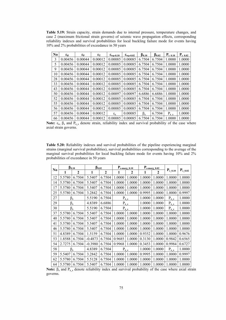
75

Table 5.19: Strain capacity, strain demands due to internal pressure, temperature changes, and case 2 (maximum frictional strain governs) of seismic wave propagation effects, corresponding reliability indexes and survival probabilities for local buckling failure mode for events having 10% and 2% probabilities of exceedance in 50 years

No εR εP εT εwp-0.10 εwp-0.02 β0.10 β0.02 Ps_0.10 Ps_0.02 3 0.00456 0.00044 0.00012 0.00085 0.00085 6.7504 6.7504 1.0000 1.00005 0.00456 0.00044 0.00012 0.00085 0.00085 6.7504 6.7504 1.0000 1.00009 0.00456 0.00044 0.00012 0.00085 0.00085 6.7504 6.7504 1.0000 1.0000

10 0.00456 0.00044 0.00012 0.00085 0.00085 6.7504 6.7504 1.0000 1.000028 0.00456 0.00044 0.00012 0.00085 0.00085 6.7504 6.7504 1.0000 1.000033 0.00456 0.00044 0.00012 0.00085 0.00085 6.7504 6.7504 1.0000 1.000043 0.00456 0.00044 0.00012 0.00085 0.00085 6.7504 6.7504 1.0000 1.000050 0.00456 0.00044 0.00012 0.00097 0.00097 6.6886 6.6886 1.0000 1.000052 0.00456 0.00044 0.00012 0.00085 0.00085 6.7504 6.7504 1.0000 1.000055 0.00456 0.00044 0.00012 0.00085 0.00085 6.7504 6.7504 1.0000 1.000056 0.00456 0.00044 0.00012 0.00085 0.00085 6.7504 6.7504 1.0000 1.000057 0.00456 0.00044 0.00012 εa 0.00085 βa 6.7504 Ps_a 1.000066 0.00456 0.00044 0.00012 0.00085 0.00085 6.7504 6.7504 1.0000 1.0000

Note: εa, βa and Ps_a denote strain, reliability index and survival probability of the case where axial strain governs. Table 5.20: Reliability indexes and survival probabilities of the pipeline experiencing marginal strains (marginal survival probabilities), survival probabilities corresponding to the average of the marginal survival probabilities for local buckling failure mode for events having 10% and 2% probabilities of exceedance in 50 years

No β0.10 β0.02 Ps-marg_0.10 Ps-marg_0.02 Ps_0.10 Ps_0.02 1 2 1 2 1 2 1 2

12 5.5780 6.7504 5.5407 6.7504 1.0000 1.0000 1.0000 1.0000 1.0000 1.000014 5.5780 6.7504 5.5407 6.7504 1.0000 1.0000 1.0000 1.0000 1.0000 1.000017 5.5780 6.7504 5.5407 6.7504 1.0000 1.0000 1.0000 1.0000 1.0000 1.000025 5.5780 6.7504 3.2842 6.7504 1.0000 1.0000 0.9995 1.0000 1.0000 0.999727 βa 5.5190 6.7504 Ps_a 1.0000 1.0000 Ps_a 1.000029 βa 4.8389 6.6886 Ps_a 1.0000 1.0000 Ps_a 1.000030 βa 5.5190 6.7504 Ps_a 1.0000 1.0000 Ps_a 1.000037 5.5780 6.7504 5.5407 6.7504 1.0000 1.0000 1.0000 1.0000 1.0000 1.000040 5.5780 6.7504 5.5407 6.7504 1.0000 1.0000 1.0000 1.0000 1.0000 1.000041 5.5780 6.7504 5.5407 6.7504 1.0000 1.0000 1.0000 1.0000 1.0000 1.000046 5.5780 6.7504 5.5407 6.7504 1.0000 1.0000 1.0000 1.0000 1.0000 1.000051 4.8389 6.7504 1.5159 6.7504 1.0000 1.0000 0.9352 1.0000 1.0000 0.967653 1.8588 6.7504 -0.4873 6.7504 0.9685 1.0000 0.3130 1.0000 0.9842 0.656554 2.7275 6.7504 -0.3980 6.7504 0.9968 1.0000 0.3453 1.0000 0.9984 0.672758 βa 4.8389 6.7504 Ps_a 1.0000 1.0000 Ps_a 1.000059 5.5407 6.7504 3.2842 6.7504 1.0000 1.0000 0.9995 1.0000 1.0000 0.999762 5.5780 6.7504 5.5128 6.7504 1.0000 1.0000 1.0000 1.0000 1.0000 1.000064 5.5780 6.7504 5.5407 6.7504 1.0000 1.0000 1.0000 1.0000 1.0000 1.0000

Note: βa and Ps_a denote reliability index and survival probability of the case where axial strain governs.

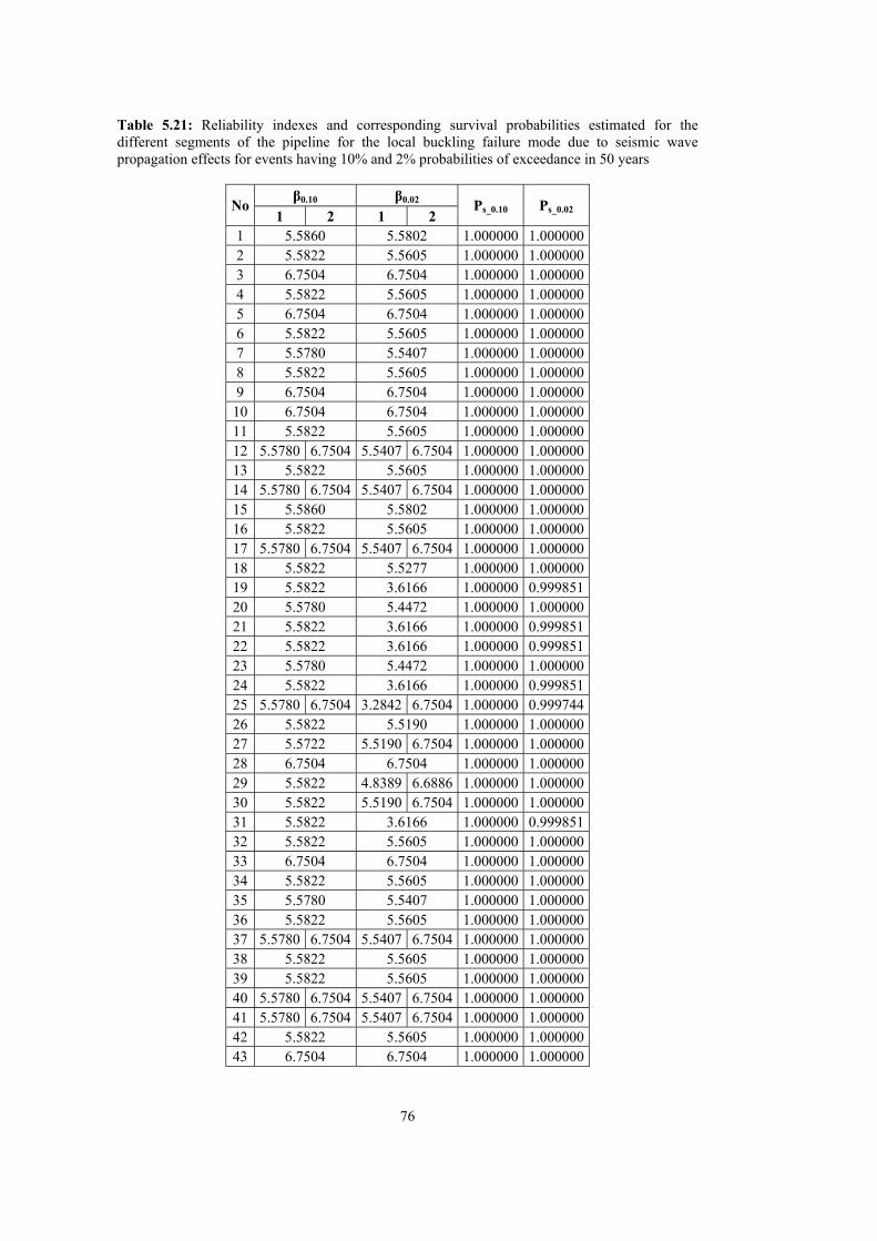
76

Table 5.21: Reliability indexes and corresponding survival probabilities estimated for the different segments of the pipeline for the local buckling failure mode due to seismic wave propagation effects for events having 10% and 2% probabilities of exceedance in 50 years

No β0.10 β0.02 Ps_0.10 Ps_0.02

1 2 1 2 1 5.5860 5.5802 1.000000 1.0000002 5.5822 5.5605 1.000000 1.0000003 6.7504 6.7504 1.000000 1.0000004 5.5822 5.5605 1.000000 1.0000005 6.7504 6.7504 1.000000 1.0000006 5.5822 5.5605 1.000000 1.0000007 5.5780 5.5407 1.000000 1.0000008 5.5822 5.5605 1.000000 1.0000009 6.7504 6.7504 1.000000 1.000000

10 6.7504 6.7504 1.000000 1.00000011 5.5822 5.5605 1.000000 1.00000012 5.5780 6.7504 5.5407 6.7504 1.000000 1.00000013 5.5822 5.5605 1.000000 1.00000014 5.5780 6.7504 5.5407 6.7504 1.000000 1.00000015 5.5860 5.5802 1.000000 1.00000016 5.5822 5.5605 1.000000 1.00000017 5.5780 6.7504 5.5407 6.7504 1.000000 1.00000018 5.5822 5.5277 1.000000 1.00000019 5.5822 3.6166 1.000000 0.99985120 5.5780 5.4472 1.000000 1.00000021 5.5822 3.6166 1.000000 0.99985122 5.5822 3.6166 1.000000 0.99985123 5.5780 5.4472 1.000000 1.00000024 5.5822 3.6166 1.000000 0.99985125 5.5780 6.7504 3.2842 6.7504 1.000000 0.99974426 5.5822 5.5190 1.000000 1.00000027 5.5722 5.5190 6.7504 1.000000 1.00000028 6.7504 6.7504 1.000000 1.00000029 5.5822 4.8389 6.6886 1.000000 1.00000030 5.5822 5.5190 6.7504 1.000000 1.00000031 5.5822 3.6166 1.000000 0.99985132 5.5822 5.5605 1.000000 1.00000033 6.7504 6.7504 1.000000 1.00000034 5.5822 5.5605 1.000000 1.00000035 5.5780 5.5407 1.000000 1.00000036 5.5822 5.5605 1.000000 1.00000037 5.5780 6.7504 5.5407 6.7504 1.000000 1.00000038 5.5822 5.5605 1.000000 1.00000039 5.5822 5.5605 1.000000 1.00000040 5.5780 6.7504 5.5407 6.7504 1.000000 1.00000041 5.5780 6.7504 5.5407 6.7504 1.000000 1.00000042 5.5822 5.5605 1.000000 1.00000043 6.7504 6.7504 1.000000 1.000000

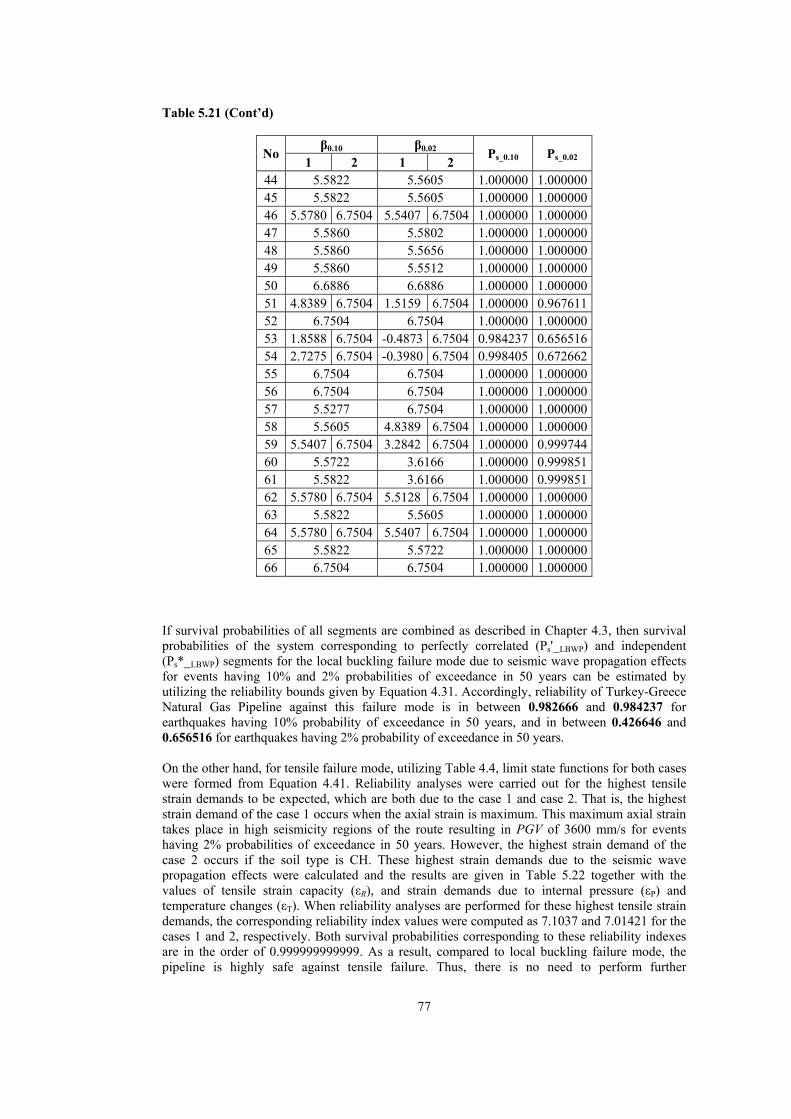
77


No β0.10 β0.02 Ps_0.10 Ps_0.02 1 2 1 2

44 5.5822 5.5605 1.000000 1.000000 45 5.5822 5.5605 1.000000 1.000000 46 5.5780 6.7504 5.5407 6.7504 1.000000 1.000000 47 5.5860 5.5802 1.000000 1.000000 48 5.5860 5.5656 1.000000 1.000000 49 5.5860 5.5512 1.000000 1.000000 50 6.6886 6.6886 1.000000 1.000000 51 4.8389 6.7504 1.5159 6.7504 1.000000 0.967611 52 6.7504 6.7504 1.000000 1.000000 53 1.8588 6.7504 -0.4873 6.7504 0.984237 0.656516 54 2.7275 6.7504 -0.3980 6.7504 0.998405 0.672662 55 6.7504 6.7504 1.000000 1.000000 56 6.7504 6.7504 1.000000 1.000000 57 5.5277 6.7504 1.000000 1.000000 58 5.5605 4.8389 6.7504 1.000000 1.000000 59 5.5407 6.7504 3.2842 6.7504 1.000000 0.999744 60 5.5722 3.6166 1.000000 0.999851 61 5.5822 3.6166 1.000000 0.999851 62 5.5780 6.7504 5.5128 6.7504 1.000000 1.000000 63 5.5822 5.5605 1.000000 1.000000 64 5.5780 6.7504 5.5407 6.7504 1.000000 1.000000 65 5.5822 5.5722 1.000000 1.000000 66 6.7504 6.7504 1.000000 1.000000

If survival probabilities of all segments are combined as described in Chapter 4.3, then survival probabilities of the system corresponding to perfectly correlated (Ps'_LBWP) and independent (Ps*_LBWP) segments for the local buckling failure mode due to seismic wave propagation effects for events having 10% and 2% probabilities of exceedance in 50 years can be estimated by utilizing the reliability bounds given by Equation 4.31. Accordingly, reliability of Turkey-Greece Natural Gas Pipeline against this failure mode is in between 0.982666 and 0.984237 for earthquakes having 10% probability of exceedance in 50 years, and in between 0.426646 and 0.656516 for earthquakes having 2% probability of exceedance in 50 years. On the other hand, for tensile failure mode, utilizing Table 4.4, limit state functions for both cases were formed from Equation 4.41. Reliability analyses were carried out for the highest tensile strain demands to be expected, which are both due to the case 1 and case 2. That is, the highest strain demand of the case 1 occurs when the axial strain is maximum. This maximum axial strain takes place in high seismicity regions of the route resulting in PGV of 3600 mm/s for events having 2% probabilities of exceedance in 50 years. However, the highest strain demand of the case 2 occurs if the soil type is CH. These highest strain demands due to the seismic wave propagation effects were calculated and the results are given in Table 5.22 together with the values of tensile strain capacity (εR), and strain demands due to internal pressure (εP) and temperature changes (εT). When reliability analyses are performed for these highest tensile strain demands, the corresponding reliability index values were computed as 7.1037 and 7.01421 for the cases 1 and 2, respectively. Both survival probabilities corresponding to these reliability indexes are in the order of 0.999999999999. As a result, compared to local buckling failure mode, the pipeline is highly safe against tensile failure. Thus, there is no need to perform further

78

computations for the tensile failure mode. Consequently, reliability of the pipeline against local buckling failure mode mentioned above can be adopted as the reliability of the pipeline subjected to wave propagation effects. Table 5.22: Strain capacity, strain demands due to internal pressure, and temperature changes, highest tensile strain demands due to case 1 (axial strain governs) and case 2 (maximum frictional strain governs) of seismic wave propagation effects for events having 2% probabilities of exceedance in 50 years

Case εR εP εT εwp-0.02

εa governs 0.04 0.00044 0.00012 0.00667

εmax governs 0.04 0.00044 0.00012 0.00675

The results indicate that the reliability of the pipeline in local buckling failure mode is not critical for the Functional Evaluation Earthquake (FEE), i.e. events having 10% probabilities of exceedance in 50 years. However for Safety Evaluation Earthquake (SEE), i.e. events having 2% probabilities of exceedance in 50 years, the pipeline may fail with significant probability especially in the regions of high seismicity. This probability may be decreased by reducing the friction between the pipe and soil. This may be achieved by selecting backfill soil of cohesionless type, instead of claylike cohesive soils; or the pipe wall thickness may be increased to enhance the reliability of the pipeline in regions of high seismicity and cohesive soils.

5.3.2LoadduetoPermanentGroundDeformationEffects As discussed in Chapter 3, compared to wave propagation hazards, permanent ground deformation (PGD) hazards have higher potential risk for buried pipelines. Thus, PGD hazards should be taken into consideration in the design stage of buried pipelines in order to mitigate the detrimental effects to pipelines. Among PGD hazards, liquefaction induced lateral spreading, liquefaction induced buoyancy and fault crossing effects to buried pipelines are considered in this study. To illustrate the implementation of the proposed methodology, the reliability of Turkey-Greece Natural Gas Pipeline is assessed against these PGD hazards.

5.3.2.1LoadduetoLiquefactionInducedLateralSpreading In order to have lateral spreading, first liquefaction has to occur. This is true for other liquefaction induced events like buoyancy. In this context, when liquefaction occurs, lateral spreading may occur in two different ways with respect to the orientation of the pipeline. These are longitudinal and transverse PGD cases. Turkey-Greece Natural Gas Pipeline was evaluated in terms of liquefaction risk in the design stage. According to BOTAŞ (2003) technical documents, there is one region possessing a very high liquefaction risk in the route of the pipeline. It is the region dashed in green near the Saros-

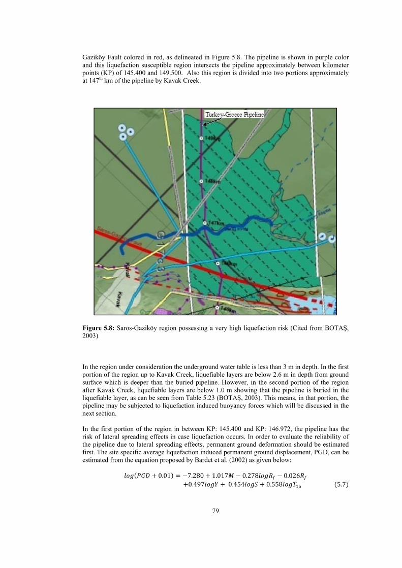
79

Gaziköy Fault colored in red, as delineated in Figure 5.8. The pipeline is shown in purple color and this liquefaction susceptible region intersects the pipeline approximately between kilometer points (KP) of 145.400 and 149.500. Also this region is divided into two portions approximately at 147th km of the pipeline by Kavak Creek.

Figure 5.8: Saros-Gaziköy region possessing a very high liquefaction risk (Cited from BOTAŞ, 2003) In the region under consideration the underground water table is less than 3 m in depth. In the first portion of the region up to Kavak Creek, liquefiable layers are below 2.6 m in depth from ground surface which is deeper than the buried pipeline. However, in the second portion of the region after Kavak Creek, liquefiable layers are below 1.0 m showing that the pipeline is buried in the liquefiable layer, as can be seen from Table 5.23 (BOTAŞ, 2003). This means, in that portion, the pipeline may be subjected to liquefaction induced buoyancy forces which will be discussed in the next section. In the first portion of the region in between KP: 145.400 and KP: 146.972, the pipeline has the risk of lateral spreading effects in case liquefaction occurs. In order to evaluate the reliability of the pipeline due to lateral spreading effects, permanent ground deformation should be estimated first. The site specific average liquefaction induced permanent ground displacement, PGD, can be estimated from the equation proposed by Bardet et al. (2002) as given below: 0.01 7.280 1.017 0.278 0.026 0.497 0.454 0.558 5.7

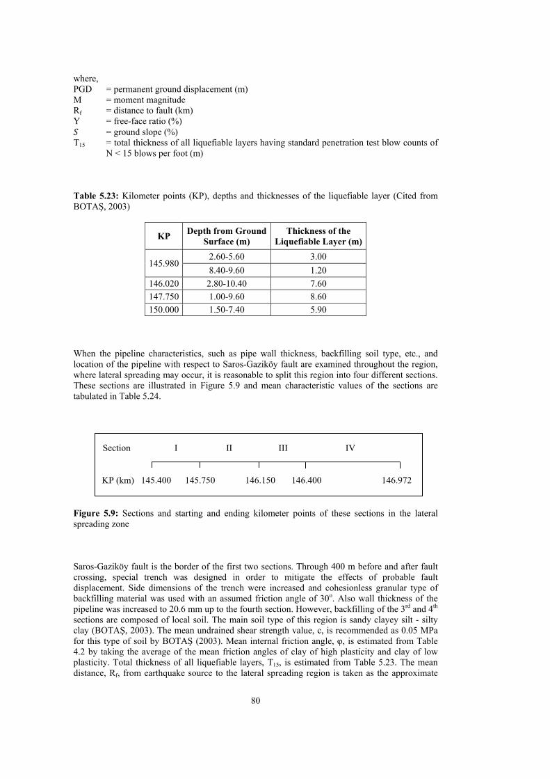
80

where, PGD = permanent ground displacement (m) M = moment magnitude Rf = distance to fault (km) Y = free-face ratio (%)

= ground slope (%) T15 = total thickness of all liquefiable layers having standard penetration test blow counts of

N < 15 blows per foot (m) Table 5.23: Kilometer points (KP), depths and thicknesses of the liquefiable layer (Cited from BOTAŞ, 2003)

KP Depth from Ground

Surface (m) Thickness of the

Liquefiable Layer (m)

145.980 2.60-5.60 3.00

8.40-9.60 1.20

146.020 2.80-10.40 7.60

147.750 1.00-9.60 8.60

150.000 1.50-7.40 5.90 When the pipeline characteristics, such as pipe wall thickness, backfilling soil type, etc., and location of the pipeline with respect to Saros-Gaziköy fault are examined throughout the region, where lateral spreading may occur, it is reasonable to split this region into four different sections. These sections are illustrated in Figure 5.9 and mean characteristic values of the sections are tabulated in Table 5.24.

Figure 5.9: Sections and starting and ending kilometer points of these sections in the lateral spreading zone Saros-Gaziköy fault is the border of the first two sections. Through 400 m before and after fault crossing, special trench was designed in order to mitigate the effects of probable fault displacement. Side dimensions of the trench were increased and cohesionless granular type of backfilling material was used with an assumed friction angle of 30o. Also wall thickness of the pipeline was increased to 20.6 mm up to the fourth section. However, backfilling of the 3rd and 4th sections are composed of local soil. The main soil type of this region is sandy clayey silt - silty clay (BOTAŞ, 2003). The mean undrained shear strength value, c, is recommended as 0.05 MPa for this type of soil by BOTAŞ (2003). Mean internal friction angle, φ, is estimated from Table 4.2 by taking the average of the mean friction angles of clay of high plasticity and clay of low plasticity. Total thickness of all liquefiable layers, T15, is estimated from Table 5.23. The mean distance, Rf, from earthquake source to the lateral spreading region is taken as the approximate

Section I II III IV

KP (km) 145.400 145.750 146.150 146.400 146.972

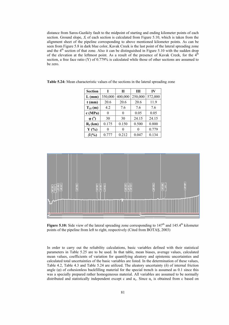
distance frsection. Galignmentseen fromand the 4t

of the elesection, a be zero. Table 5.2

Figure 5.points of t In order tparametermean valucalculatedTable 4.2,angle (φ) was a spedistributed

from Saros-GaGround slope, t sheet of the

m Figure 5.8 inth section of thevation at the

free face ratio

4: Mean char

10: Side viewthe pipeline fr

to carry out rs in Table 5.ues, coefficien

d total uncerta, Table 4.3 anof cohesionle

ecially prepared and statistic

aziköy fault toS, of each secpipeline corr

n dark blue colhat zone. Also

leftmost poino (Y) of 0.779

acteristic valu

Section

L (mm) 3

t (mm)

T15 (m)

c (MPa)

φ (o)

Rf (km)

Y (%) S (%)

w of the lateralrom left to righ

the reliability25 are to be nts of variati

ainties of the bnd Table 5.24ess backfillinged rather homcally independ

81

o the midpointction is calculresponding tolor, Kavak Cro it can be disnt. As a resu9% is calculat

ues of the sect

I II

50,000 400,0

20.6 20.

4.2 7.6

0 0

30 30

0.175 0.15

0 0

0.777 0.21

l spreading zoht, respectivel

y calculationsused. In that on for quanti

basic variables4 are utilized. g material for

mogeneous matdent except c

1

t of starting anlated from Fig

o above mentireek is the laststinguished in

ult of the prested while thos

ions in the lat

I III

000 250,000

.6 20.6

6 7.6

0.05

0 24.15

50 0.500

0

12 0.047

one corresponly (Cited from

s, basic variatable, mean

ifying aleatorys are listed. InThe aleatory

r the special trterial. All var

c and αc. Sinc

nd ending kilogure 5.10, whioned kilomett point of the ln Figure 5.10 sence of Kavse of other sec

teral spreading

IV

572,000

11.9

7.6

0.05

24.15

0.800

0.779

0.134

ding to 147th m BOTAŞ, 200

ables defined biases, averay and epistem

n the determinuncertainty (δrench is assumriables are assce αc is obtain

ometer pointshich is taken fter points. Aslateral spreadiwith the suddak Creek, forctions are assu

g zone

and 145.4th ki03)

with their stage values, camic uncertaintnation of theseδ) of internal med as 0.1 sisumed to be nned from c b

of each from the s can be ing zone den drop r the 4th umed to

ilometer

tatistical alculated ties and

e values, friction

ince this normally based on

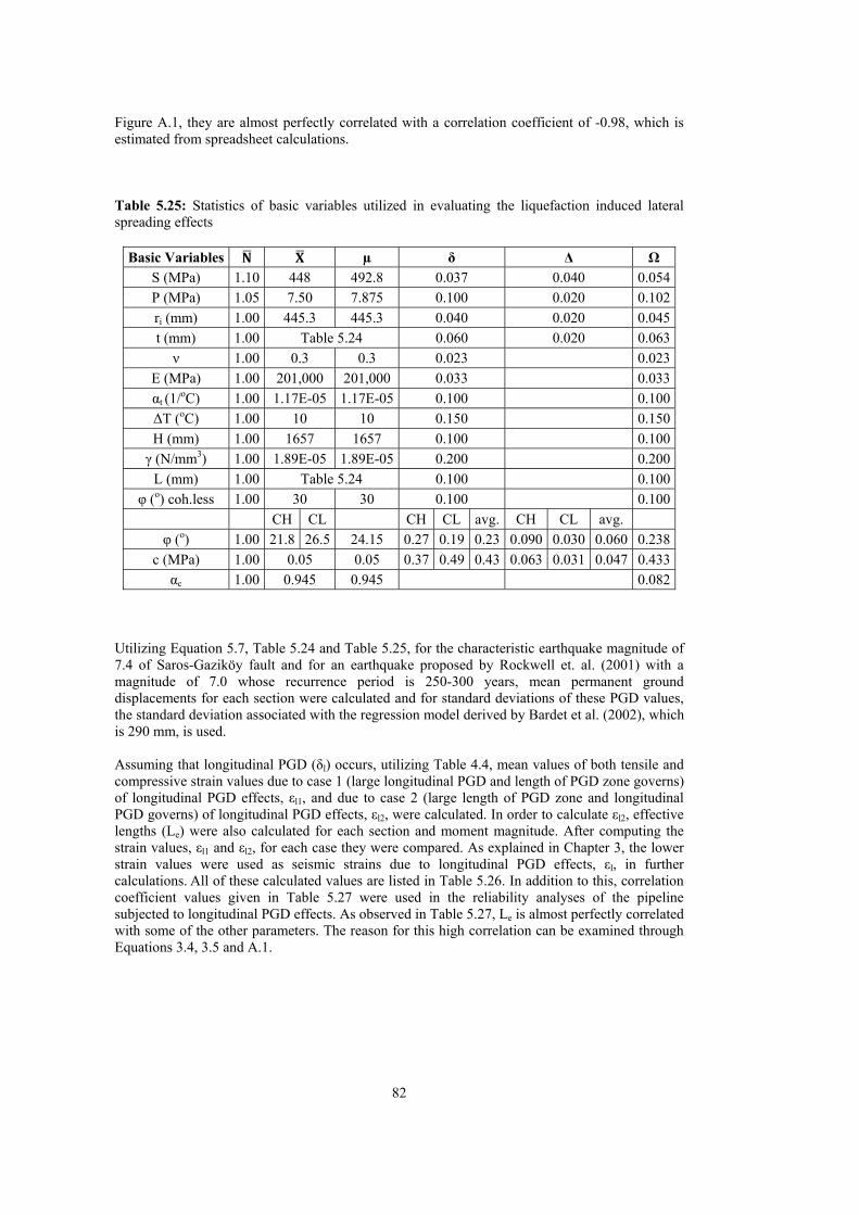
82

Figure A.1, they are almost perfectly correlated with a correlation coefficient of -0.98, which is estimated from spreadsheet calculations. Table 5.25: Statistics of basic variables utilized in evaluating the liquefaction induced lateral spreading effects

Basic Variables µ δ Δ Ω S (MPa) 1.10 448 492.8 0.037 0.040 0.054

P (MPa) 1.05 7.50 7.875 0.100 0.020 0.102

ri (mm) 1.00 445.3 445.3 0.040 0.020 0.045

t (mm) 1.00 Table 5.24 0.060 0.020 0.063

ν 1.00 0.3 0.3 0.023 0.023

E (MPa) 1.00 201,000 201,000 0.033 0.033

αt (1/oC) 1.00 1.17E-05 1.17E-05 0.100 0.100

ΔT (oC) 1.00 10 10 0.150 0.150

H (mm) 1.00 1657 1657 0.100 0.100

γ (N/mm3) 1.00 1.89E-05 1.89E-05 0.200 0.200

L (mm) 1.00 Table 5.24 0.100 0.100

φ (o) coh.less 1.00 30 30 0.100 0.100

CH CL CH CL avg. CH CL avg.

φ (o) 1.00 21.8 26.5 24.15 0.27 0.19 0.23 0.090 0.030 0.060 0.238

c (MPa) 1.00 0.05 0.05 0.37 0.49 0.43 0.063 0.031 0.047 0.433

αc 1.00 0.945 0.945 0.082 Utilizing Equation 5.7, Table 5.24 and Table 5.25, for the characteristic earthquake magnitude of 7.4 of Saros-Gaziköy fault and for an earthquake proposed by Rockwell et. al. (2001) with a magnitude of 7.0 whose recurrence period is 250-300 years, mean permanent ground displacements for each section were calculated and for standard deviations of these PGD values, the standard deviation associated with the regression model derived by Bardet et al. (2002), which is 290 mm, is used. Assuming that longitudinal PGD (δl) occurs, utilizing Table 4.4, mean values of both tensile and compressive strain values due to case 1 (large longitudinal PGD and length of PGD zone governs) of longitudinal PGD effects, εl1, and due to case 2 (large length of PGD zone and longitudinal PGD governs) of longitudinal PGD effects, εl2, were calculated. In order to calculate εl2, effective lengths (Le) were also calculated for each section and moment magnitude. After computing the strain values, εl1 and εl2, for each case they were compared. As explained in Chapter 3, the lower strain values were used as seismic strains due to longitudinal PGD effects, εl, in further calculations. All of these calculated values are listed in Table 5.26. In addition to this, correlation coefficient values given in Table 5.27 were used in the reliability analyses of the pipeline subjected to longitudinal PGD effects. As observed in Table 5.27, Le is almost perfectly correlated with some of the other parameters. The reason for this high correlation can be examined through Equations 3.4, 3.5 and A.1.

83

Table 5.26: Means and standard deviations of longitudinal PGD and effective length, mean strains for cases 1 and 2 of longitudinal PGD effects and the seismic strains due to longitudinal PGD effects in each section for M=7.4 and M=7.0

Section M µδl (mm) σδl (mm) µLe (mm) σLe (mm) εl1 εl2 εl

I 7.4 5610 290 1,499,270 84,431 0.00032 0.01100 0.000327.0 2192 290 1,089,062 27,771 0.00032 0.00206 0.00032

II 7.4 4525 290 1,437,444 74,675 0.00037 0.00689 0.000377.0 1767 290 978,962 18,600 0.00037 0.00181 0.00037

III 7.4 1594 290 232,171 22,346 0.00200 0.03600 0.002007.0 619 290 202,440 12,450 0.00200 0.00628 0.00200

IV 7.4 1954 290 142,776 14,135 5,989 0.09200 0.092007.0 760 290 131,539 12,273 5,989 0.02700 0.02700

Table 5.27: Correlation coefficient matrix used in the estimation of the reliability index corresponding to case 2 of longitudinal PGD effects

Sy ri t P ν E αt ΔT φ H γ c αc Le

Sy 1.00 0.00 0.00 0.00 0.00 0.00 0.00 0.00 0.00 0.00 0.00 0.00 0.00 0.98

ri 0.00 1.00 0.00 0.00 0.00 0.00 0.00 0.00 0.00 0.00 0.00 0.00 0.00 0.00

t 0.00 0.00 1.00 0.00 0.00 0.00 0.00 0.00 0.00 0.00 0.00 0.00 0.00 1.00P 0.00 0.00 0.00 1.00 0.00 0.00 0.00 0.00 0.00 0.00 0.00 0.00 0.00 0.00ν 0.00 0.00 0.00 0.00 1.00 0.00 0.00 0.00 0.00 0.00 0.00 0.00 0.00 0.00E 0.00 0.00 0.00 0.00 0.00 1.00 0.00 0.00 0.00 0.00 0.00 0.00 0.00 1.00

αt 0.00 0.00 0.00 0.00 0.00 0.00 1.00 0.00 0.00 0.00 0.00 0.00 0.00 0.00

ΔT 0.00 0.00 0.00 0.00 0.00 0.00 0.00 1.00 0.00 0.00 0.00 0.00 0.00 0.00

φ 0.00 0.00 0.00 0.00 0.00 0.00 0.00 0.00 1.00 0.00 0.00 0.00 0.00 -1.00H 0.00 0.00 0.00 0.00 0.00 0.00 0.00 0.00 0.00 1.00 0.00 0.00 0.00 -1.00γ 0.00 0.00 0.00 0.00 0.00 0.00 0.00 0.00 0.00 0.00 1.00 0.00 0.00 -1.00c 0.00 0.00 0.00 0.00 0.00 0.00 0.00 0.00 0.00 0.00 0.00 1.00 -0.98 -0.96

αc 0.00 0.00 0.00 0.00 0.00 0.00 0.00 0.00 0.00 0.00 0.00 -0.98 1.00 0.00

Le 0.98 0.00 1.00 0.00 0.00 1.00 0.00 0.00 -1.00 -1.00 -1.00 -0.96 0.00 1.00

In order to carry out reliability analyses, utilizing Table 4.4, safety margins, which are defined by Equation 4.41, and which correspond to tensile and local buckling failure modes due to each cases of longitudinal PGD effects, were formed. After these rigorous analyses, the results, corresponding to tensile and local buckling failure modes due to longitudinal PGD effects, are given in Tables 5.28 and 5.29, respectively. It can be seen from these tables that first two sections are almost perfectly reliable to resist lateral spreading effect when liquefaction occurs. Also in these sections just tensile failure mode is applicable because accompanied with loads due to internal pressure and temperature differences, longitudinal PGD effects cannot form compressive strains in the pipeline.

84

Table 5.28: Strain capacity, strain demands due to internal pressure, temperature changes, and longitudinal PGD, safety margins, reliability indexes and survival probabilities of the pipeline corresponding to tensile failure mode due to longitudinal PGD effects in each section for M=7.4 and M=7.0

Section M εR εP εT εl Mt_LPGD βHL Ps_t

I 7.4 0.04 0.00025 0.00012 0.00032 0.03931 8.5903 1.00000

7.0 0.04 0.00025 0.00012 0.00032 0.03931 8.5903 1.00000

II 7.4 0.04 0.00025 0.00012 0.00037 0.03927 8.6863 1.00000

7.0 0.04 0.00025 0.00012 0.00037 0.03927 8.6863 1.00000

III 7.4 0.04 0.00025 0.00012 0.00200 0.03801 2.6065 0.99543

7.0 0.04 0.00025 0.00012 0.00200 0.03801 2.6065 0.99543

IV 7.4 0.04 0.00044 0.00012 0.09200 -0.05287 -0.1002 0.46009

7.0 0.04 0.00044 0.00012 0.02700 0.01248 0.0506 0.52018 Table 5.29: Strain capacity, strain demands due to internal pressure, temperature changes, and longitudinal PGD, safety margins, reliability indexes and survival probabilities of the pipeline corresponding to local buckling failure mode due to longitudinal PGD effects in each section for M=7.4 and M=7.0

Section M εR εP εT εl Mc_LPGD βHL Ps_lb

I 7.4 0.00789 0.00025 0.00012 0.00032 no net compressive strain

7.0 0.00789 0.00025 0.00012 0.00032 no net compressive strain

II 7.4 0.00789 0.00025 0.00012 0.00037 no net compressive strain

7.0 0.00789 0.00025 0.00012 0.00037 no net compressive strain

III 7.4 0.00789 0.00025 0.00012 0.00200 0.00663 1.9768 0.97597

7.0 0.00789 0.00025 0.00012 0.00200 0.00663 1.9768 0.97597

IV 7.4 0.00456 0.00044 0.00012 0.09200 -0.08721 -0.3740 0.35420

7.0 0.00456 0.00044 0.00012 0.02700 -0.02185 -0.2559 0.39901 These calculations were made to analyze the pipeline subjected to longitudinal PGD effects. However, in that region susceptible to lateral spreading, transverse PGD (δt) may also occur in accordance with the orientation of the pipeline. When topographic map of this region, illustrated in Figure 5.11, is examined, it can be inferred that the pipeline may also be subjected to transverse PGD effects because of the orientation of contour lines. That is why the pipeline passing throughout that region is also analyzed against transverse PGD effects. In the reliability analyses of the pipeline subjected to transverse PGD effects, the same sections used in longitudinal PGD analyses are utilized. Also in account of the similarities of the topographies, the same permanent ground displacements are assumed to occur in case liquefaction induced lateral spreading takes place. Moreover, lengths of sections given in Table 5.24 are assumed to be the width (W) of the transverse PGD zone. The statistics of basic variables in Table 5.25 are used to carry out the reliability analyses.

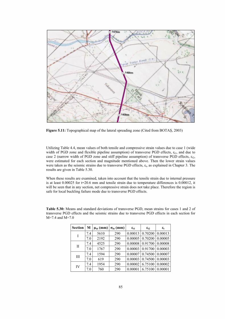
85

Figure 5.11: Topographical map of the lateral spreading zone (Cited from BOTAŞ, 2003) Utilizing Table 4.4, mean values of both tensile and compressive strain values due to case 1 (wide width of PGD zone and flexible pipeline assumption) of transverse PGD effects, εt1, and due to case 2 (narrow width of PGD zone and stiff pipeline assumption) of transverse PGD effects, εt2, were estimated for each section and magnitude mentioned above. Then the lower strain values were taken as the seismic strains due to transverse PGD effects, εt, as explained in Chapter 3. The results are given in Table 5.30. When these results are examined, taken into account that the tensile strain due to internal pressure is at least 0.00025 for t=20.6 mm and tensile strain due to temperature differences is 0.00012, it will be seen that in any section, net compressive strain does not take place. Therefore the region is safe for local buckling failure mode due to transverse PGD effects. Table 5.30: Means and standard deviations of transverse PGD, mean strains for cases 1 and 2 of transverse PGD effects and the seismic strains due to transverse PGD effects in each section for M=7.4 and M=7.0

Section M µδt (mm) σδt (mm) εt1 εt2 εt

I 7.4 5610 290 0.00013 0.70200 0.00013 7.0 2192 290 0.00005 0.70200 0.00005

II 7.4 4525 290 0.00008 0.91700 0.00008

7.0 1767 290 0.00003 0.91700 0.00003

III 7.4 1594 290 0.00007 0.74500 0.00007 7.0 619 290 0.00003 0.74500 0.00003

IV 7.4 1954 290 0.00002 6.75100 0.00002 7.0 760 290 0.00001 6.75100 0.00001

86

Reliability analyses were carried out also for the tensile failure mode. Strain values in Table 5.30 show that case 1 of transverse PGD effects is dominant in all situations. Then, from Equation 4.41, safety margins were formed and reliability indexes and corresponding survival probabilities were calculated as given in Table 5.31. Table 5.31: Strain capacity, strain demands due to internal pressure, temperature changes, and transverse PGD, safety margins, reliability indexes and survival probabilities of the pipeline corresponding to tensile failure mode due to transverse PGD effects in each section for M=7.4 and M=7.0

Section M εR εP εT εt Mt_TPGD βHL Ps_t

I 7.4 0.04 0.00025 0.00012 0.00013 0.03950 8.2954 1.00000

7.0 0.04 0.00025 0.00012 0.00005 0.03958 8.2957 1.00000

II 7.4 0.04 0.00025 0.00012 0.00008 0.03955 8.2956 1.00000

7.0 0.04 0.00025 0.00012 0.00003 0.03960 8.2957 1.00000

III 7.4 0.04 0.00025 0.00012 0.00007 0.03956 8.2956 1.00000

7.0 0.04 0.00025 0.00012 0.00003 0.03961 8.2957 1.00000

IV 7.4 0.04 0.00044 0.00012 0.00002 0.03943 8.2937 1.00000

7.0 0.04 0.00044 0.00012 0.00001 0.03944 8.2937 1.00000 As mentioned before, lateral spreading occurs given that liquefaction takes place. Accordingly, in order to evaluate the reliability of the pipeline due to liquefaction induced lateral spreading, the probability of the liquefaction has to be estimated. For this purpose, ALA Guideline (2005) proposes an easy method to calculate the probability of liquefaction provided that the liquefaction susceptibility of the region considered is known. The probability of liquefaction can be estimated from the equation given below: | 5.8

where, | = probability of liquefaction given a specified peak ground

acceleration (PGA) in g (see Table 5.32) Km = moment magnitude correction factor (see Equation 5.9) Kw = ground water correction factor (see Equation 5.10) Pml = proportion of the map unit susceptible to liquefaction (see Table 5.33) 0.0027 0.0267 0.2055 2.9188 5.9 where, M = moment magnitude 0.022 0.93 5.10 where, dw = groundwater depth (in feet)

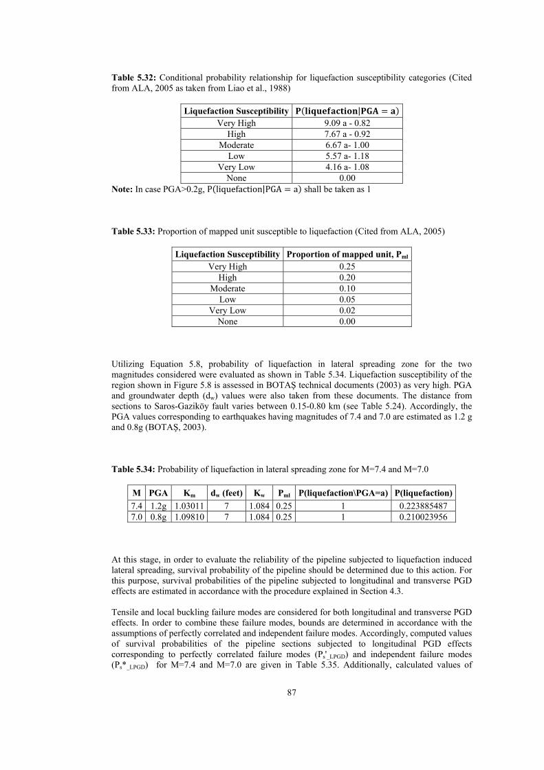
87

Table 5.32: Conditional probability relationship for liquefaction susceptibility categories (Cited from ALA, 2005 as taken from Liao et al., 1988)

Liquefaction Susceptibility | Very High 9.09 a - 0.82

High 7.67 a - 0.92 Moderate 6.67 a- 1.00

Low 5.57 a- 1.18 Very Low 4.16 a- 1.08

None 0.00 Note: In case PGA>0.2g, P liquefaction|PGA a shall be taken as 1 Table 5.33: Proportion of mapped unit susceptible to liquefaction (Cited from ALA, 2005)

Liquefaction Susceptibility Proportion of mapped unit, Pml Very High 0.25

High 0.20 Moderate 0.10

Low 0.05 Very Low 0.02

None 0.00 Utilizing Equation 5.8, probability of liquefaction in lateral spreading zone for the two magnitudes considered were evaluated as shown in Table 5.34. Liquefaction susceptibility of the region shown in Figure 5.8 is assessed in BOTAŞ technical documents (2003) as very high. PGA and groundwater depth (dw) values were also taken from these documents. The distance from sections to Saros-Gaziköy fault varies between 0.15-0.80 km (see Table 5.24). Accordingly, the PGA values corresponding to earthquakes having magnitudes of 7.4 and 7.0 are estimated as 1.2 g and 0.8g (BOTAŞ, 2003). Table 5.34: Probability of liquefaction in lateral spreading zone for M=7.4 and M=7.0

M PGA Km dw (feet) Kw Pml P(liquefaction\PGA=a) P(liquefaction)

7.4 1.2g 1.03011 7 1.084 0.25 1 0.223885487 7.0 0.8g 1.09810 7 1.084 0.25 1 0.210023956

At this stage, in order to evaluate the reliability of the pipeline subjected to liquefaction induced lateral spreading, survival probability of the pipeline should be determined due to this action. For this purpose, survival probabilities of the pipeline subjected to longitudinal and transverse PGD effects are estimated in accordance with the procedure explained in Section 4.3. Tensile and local buckling failure modes are considered for both longitudinal and transverse PGD effects. In order to combine these failure modes, bounds are determined in accordance with the assumptions of perfectly correlated and independent failure modes. Accordingly, computed values of survival probabilities of the pipeline sections subjected to longitudinal PGD effects corresponding to perfectly correlated failure modes (Ps'_LPGD) and independent failure modes (Ps*_LPGD) for M=7.4 and M=7.0 are given in Table 5.35. Additionally, calculated values of

88

survival probabilities of the pipeline sections subjected to transverse PGD effects corresponding to perfectly correlated failure modes (Ps'_TPGD) and independent failure modes (Ps*_TPGD) for M=7.4 and M=7.0 are given in Table 5.36. Table 5.35: Survival probabilities of the pipeline sections with respect to longitudinal PGD effects, assuming perfectly correlated and independent failure modes for M=7.4 and M=7.0

Section M Ps_t Ps_lb Ps'_LPGD Ps*_LPGD

I 7.4 1.000000 NA 1.000000 1.0000007.0 1.000000 NA 1.000000 1.000000

II 7.4 1.000000 NA 1.000000 1.000000

7.0 1.000000 NA 1.000000 1.000000

III 7.4 0.995426 0.975968 0.975968 0.971504

7.0 0.995426 0.975968 0.975968 0.971504

IV 7.4 0.460093 0.354202 0.354202 0.162966

7.0 0.520178 0.399014 0.399014 0.207558 Table 5.36: Survival probabilities of the pipeline sections with respect to transverse PGD effects, assuming perfectly correlated and independent failure modes for M=7.4 and M=7.0

Section M Ps_t Ps_lb Ps'_TPGD Ps*_TPGD

I 7.4 1.000000 NA 1.000000 1.000000

7.0 1.000000 NA 1.000000 1.000000

II 7.4 1.000000 NA 1.000000 1.000000

7.0 1.000000 NA 1.000000 1.000000

III 7.4 1.000000 NA 1.000000 1.000000

7.0 1.000000 NA 1.000000 1.000000

IV 7.4 1.000000 NA 1.000000 1.000000

7.0 1.000000 NA 1.000000 1.000000 The probabilities of occurrence of longitudinal and transverse PGD effects are assumed to be equally likely. Accordingly the survival probability of the pipeline sections subjected to lateral spreading effects corresponding to perfectly correlated (Ps'_LS) and independent failure modes (Ps*_LS) for M=7.4 and M=7.0 were calculated by taking the average values and are shown in the last two columns of Table 5.37. Then utilizing Table 5.37 and considering all four sections, survival probabilities of the pipeline in lateral spreading zone corresponding to perfectly correlated (Pss'_LS) and independent sections (Pss*_LS) for the magnitudes of 7.4 and 7.0 were calculated and the results are tabulated in Table 5.38. Lastly, using the probability values given in Tables 5.34 and 5.38, conservative estimates of survival probability for the pipeline in lateral spreading zone corresponding to independent sections (Pss*_LS) for the magnitudes of 7.4 and 7.0 were taken and reliability of the pipeline

89

subjected to liquefaction induced lateral spreading effects, Ps_LILS, was calculated from the following expression: _ 1 1 _∗ 5.11 Table 5.37: Survival probabilities (as average of longitudinal and transverse PGD effects) of the pipeline sections subjected to lateral spreading effects corresponding to perfectly correlated and independent failure modes for M=7.4 and M=7.0

Section M Ps'_LPGD Ps*_LPGD Ps'_TPGD Ps*_TPGD Ps'_LS Ps*_LS

I 7.4 1.000000 1.000000 1.000000 1.000000 1.000000 1.000000

7.0 1.000000 1.000000 1.000000 1.000000 1.000000 1.000000

II 7.4 1.000000 1.000000 1.000000 1.000000 1.000000 1.000000

7.0 1.000000 1.000000 1.000000 1.000000 1.000000 1.000000

III 7.4 0.975968 0.971504 1.000000 1.000000 0.987984 0.985752

7.0 0.975968 0.971504 1.000000 1.000000 0.987984 0.985752

IV 7.4 0.354202 0.162966 1.000000 1.000000 0.677101 0.581483

7.0 0.399014 0.207558 1.000000 1.000000 0.699507 0.603779 Table 5.38: Survival probabilities of the whole pipeline in lateral spreading zone corresponding to perfectly correlated and independent sections for M=7.4 and M=7.0

M Pss'_LS Pss*_LS 7.4 0.677101 0.6689657.0 0.699507 0.691102

The results are given in Table 5.39. Table 5.39: Conservative estimates of survival probability of the pipeline subjected to liquefaction induced lateral spreading for M=7.4 and M=7.0

M P(liquefaction) Pss*_LS Ps_LILS 7.4 0.223885 0.668965 0.925886 7.0 0.210024 0.691102 0.935124

The results of the reliability analyses indicate that the pipeline in the liquefaction susceptible region is subject to a significant degree of risk in case lateral spreading occurs. Since lateral spreading is the secondary event resulting from liquefaction and the likelihood of liquefaction is a rare event, the risk of liquefaction induced lateral spreading is not in the same order of magnitude as that of the lateral spreading. Yet, the reliability of the pipeline should be enhanced by taking countermeasures in order to mitigate the risk against seismic damage to the pipeline especially in the fourth section of the lateral spreading zone. Increasing pipe wall thickness and using

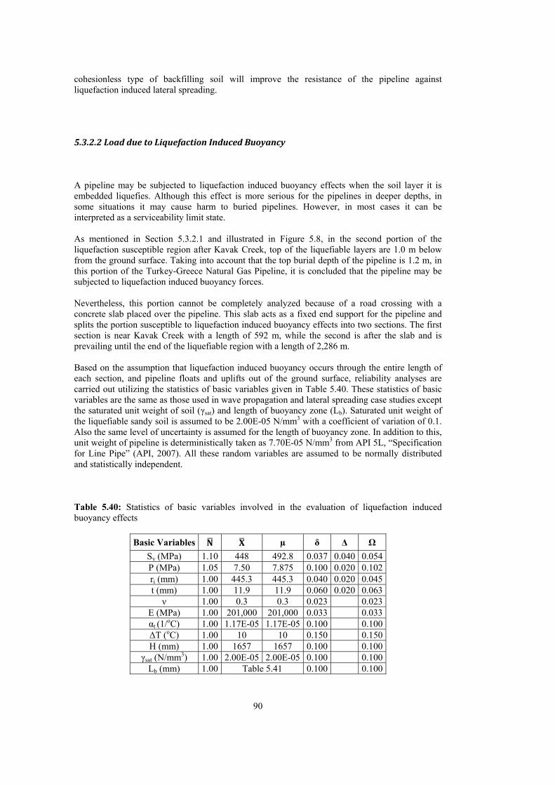
90

cohesionless type of backfilling soil will improve the resistance of the pipeline against liquefaction induced lateral spreading.

5.3.2.2LoadduetoLiquefactionInducedBuoyancy A pipeline may be subjected to liquefaction induced buoyancy effects when the soil layer it is embedded liquefies. Although this effect is more serious for the pipelines in deeper depths, in some situations it may cause harm to buried pipelines. However, in most cases it can be interpreted as a serviceability limit state. As mentioned in Section 5.3.2.1 and illustrated in Figure 5.8, in the second portion of the liquefaction susceptible region after Kavak Creek, top of the liquefiable layers are 1.0 m below from the ground surface. Taking into account that the top burial depth of the pipeline is 1.2 m, in this portion of the Turkey-Greece Natural Gas Pipeline, it is concluded that the pipeline may be subjected to liquefaction induced buoyancy forces. Nevertheless, this portion cannot be completely analyzed because of a road crossing with a concrete slab placed over the pipeline. This slab acts as a fixed end support for the pipeline and splits the portion susceptible to liquefaction induced buoyancy effects into two sections. The first section is near Kavak Creek with a length of 592 m, while the second is after the slab and is prevailing until the end of the liquefiable region with a length of 2,286 m. Based on the assumption that liquefaction induced buoyancy occurs through the entire length of each section, and pipeline floats and uplifts out of the ground surface, reliability analyses are carried out utilizing the statistics of basic variables given in Table 5.40. These statistics of basic variables are the same as those used in wave propagation and lateral spreading case studies except the saturated unit weight of soil (γsat) and length of buoyancy zone (Lb). Saturated unit weight of the liquefiable sandy soil is assumed to be 2.00E-05 N/mm3 with a coefficient of variation of 0.1. Also the same level of uncertainty is assumed for the length of buoyancy zone. In addition to this, unit weight of pipeline is deterministically taken as 7.70E-05 N/mm3 from API 5L, “Specification for Line Pipe” (API, 2007). All these random variables are assumed to be normally distributed and statistically independent. Table 5.40: Statistics of basic variables involved in the evaluation of liquefaction induced buoyancy effects


Sy (MPa) 1.10 448 492.8 0.037 0.040 0.054P (MPa) 1.05 7.50 7.875 0.100 0.020 0.102ri (mm) 1.00 445.3 445.3 0.040 0.020 0.045t (mm) 1.00 11.9 11.9 0.060 0.020 0.063

ν 1.00 0.3 0.3 0.023 0.023E (MPa) 1.00 201,000 201,000 0.033 0.033αt (1/oC) 1.00 1.17E-05 1.17E-05 0.100 0.100ΔT (oC) 1.00 10 10 0.150 0.150H (mm) 1.00 1657 1657 0.100 0.100

γsat (N/mm3) 1.00 2.00E-05 2.00E-05 0.100 0.100Lb (mm) 1.00 Table 5.41 0.100 0.100

91

Utilizing Table 4.4, tensile strain due to case 1 (narrow length of buoyancy zone and stiff pipeline assumption), εb1, and due to case 2 (large length of buoyancy zone and flexible pipeline assumption), εb2t, of liquefaction induced buoyancy effects were calculated and compared. Then the case yielding to the lower strain value was selected. As can be seen from Table 5.41, for both sections of the buoyancy zone, since the lengths of those sections are too long, case 2 gives the lower strains as expected. Because the compressive and tensile strains in case 2 are different, for local buckling failure mode, compressive strain due to case 2 of liquefaction induced buoyancy effects (εb2c) was also calculated by utilizing Table 4.4. Table 5.41: Coordinates and calculated strain values for the two sections located in the buoyancy zone

Section Start (m) End (m) Length, Lb (m) εb1 εb2t εb2c 1 147020 147612 592 1.17E+29 0.00006 0.00002 2 147636 149922 2286 6.98E+47 0 0

The results given in Table 5.41 show that in the second section, buoyancy effects resulting from liquefaction, do not create any tensile or compressive strains. Moreover, for the first section, accompanied with tensile strains due to internal pressure and temperature changes, there is no net compressive strain. Therefore the pipeline passing 592 m length of buoyancy zone is safe for local buckling failure mode. Only the tensile failure mode is checked for that section of the buoyancy zone in terms of reliability. From Equation 4.41, safety margin corresponding to tensile failure mode due to case 2 of liquefaction induced buoyancy effects was obtained. The reliability analysis gave a probability of survival value of nearly 1 (see Table 5.42), like the others mentioned above, indicating that this failure mode of liquefaction induced buoyancy also does not create any risk to Turkey-Greece Natural Gas Pipeline in terms of ultimate limit state. Thus, survival probability of the pipeline due to liquefaction induced buoyancy effects (Ps_LIB) is 1. However, for the pipeline considered, the most critical length of buoyancy is approximately 61 m. For this length of buoyancy, estimated strain value, both tensile and compressive, due to buoyancy effects is 0.00564. Taking into account that local buckling strain capacity for the pipeline having a wall thickness of 11.9 mm is 0.00456, compressive strains due to buoyancy, in the order of 0.00564, may create damage to the pipeline. However, as previously stated, such a length of liquefaction induced buoyancy is not expected along the route of the pipeline. Table 5.42: Strain capacity, strain demands due to internal pressure, temperature changes, and case 2 of liquefaction induced buoyancy effects, mean safety margin, reliability index and survival probability of the pipeline corresponding to tensile failure mode due to liquefaction induced buoyancy effects in the first section of the buoyancy zone

Section εR εP εT εb2t Mt_BUOY βHL Ps 1 0.04 0.00044 0.00012 0.00006 0.03938 8.2936 1.000000

5.3.2.3LoadduetoFaultCrossing

92

Fault crossing is one of the primary concerns in earthquake resistant design of buried continuous pipelines. Permanent ground displacements in several meters may be observed due to surface fault displacements, and this may create serious damages to buried pipelines unless necessary precautions are taken. Turkey-Greece Natural Gas Pipeline is evaluated also with respect to the effects of surface faulting in order to determine the reliability of the pipeline against this effect. In Figure 5.3, main faults in the vicinity of the pipeline are shown. When the route of the pipeline with respect to these faults is examined, it is seen that the pipeline intersects with faults at five locations. These faults and their characteristics are given in Table 5.43. Three fault crossings, Karasu (see Figure 5.12), Edincik (see Figure 5.13) and Saros-Gaziköy (see Figure 5.14), were taken into account in the design phase by BOTAŞ and the characteristics of these faults are obtained from BOTAŞ (2003). The other two fault crossings, Karacabey (see Figure 5.15) and Karabiga (see Figure 5.16), were not considered in the design phase. However, the intersection of the pipeline with these two faults, whose types are unspecified (MTA, 2011), are also taken into account in this study and the information on the characteristics of these faults is cited from the active fault map of General Directorate of Mineral Research and Exploration (MTA, 2011). Table 5.43: Information on fault crossings and characteristics of the faults that intersect the route of Turkey-Greece Natural Gas Pipeline (BOTAŞ, 2003)

Fault Name

KP Fault Type Fault

Length (km)

Estimated Magnitude

Estimated Displacement, δf (mm)

Lateral Vertical Karasu Fault Zone

5.750 Normal +

Right Lateral

5±2 6.3±0.7 0±100 500±200

Edincik Fault Zone

65.500 Right

Lateral + Normal

30±5 6.6±0.4 800±200 0±100

Saros-Gaziköy

Fault Zone

145.750 Right

Lateral

90±15 (45 at

land, 45 in sea)

7.4±0.6 5000±1000

0±1000 (due to the local movements of the lateral

fault)

Karacabey Fault

2.800 Unspecified 10 From moment

magnitude-fault length relationship

(Wells and Coppersmith,

1994)

From displacement-moment magnitude

relationship (Wells and Coppersmith, 1994) Karabiga

Fault 108.000 Unspecified 10

Since fault types are not specified for Karacabey and Karabiga faults, these are assumed to be of strike slip type. The lengths of these faults, which are estimated from the fault maps as 10 km for both of them, are substituted into Wells and Coppersmith (1994) rupture length - magnitude relationship for strike slip type of faults, and the moment magnitudes were estimated as 6.28. This equation is shown below. 5.16 1.12 5.12 where, M = moment magnitude SRL = surface rupture length

Figure 5.1

Figure 5.1

12: Karasu fau

13: Edincik fa

ult crossing (a

ault crossing (

93

as modified fr

(as modified fr

3

rom BOTAŞ, 2

from MTA, 20

2003)

011)

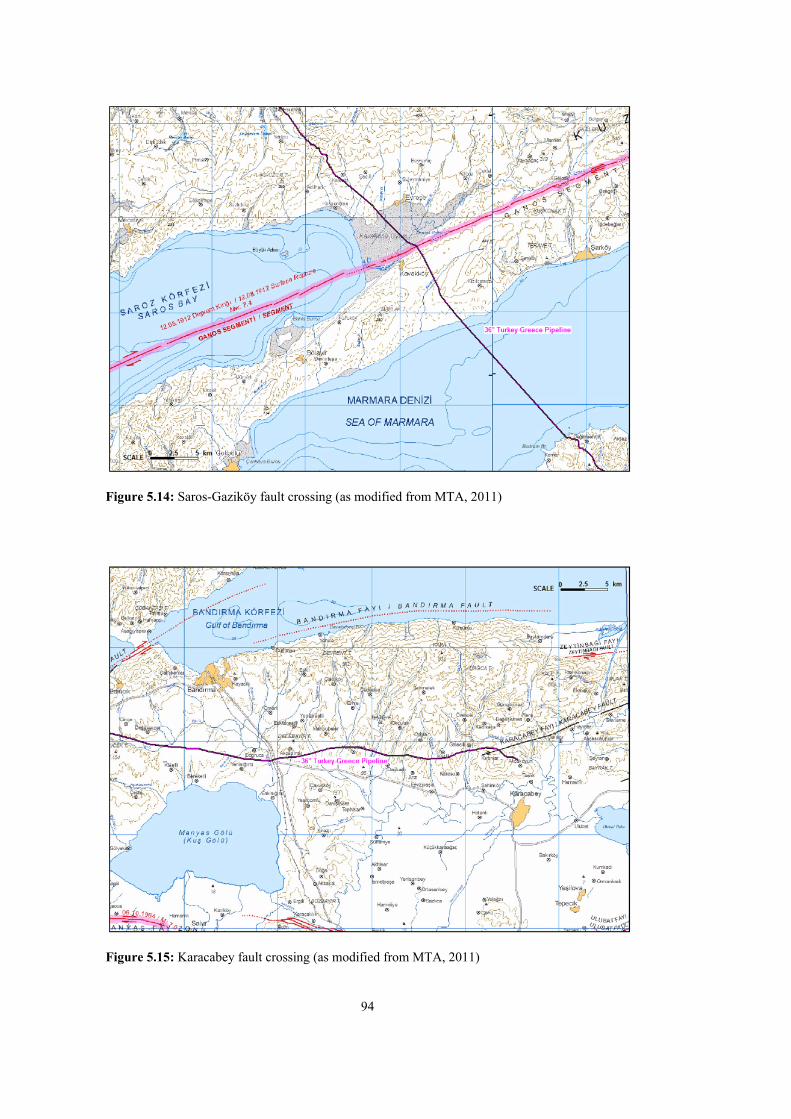
94

Figure 5.14: Saros-Gaziköy fault crossing (as modified from MTA, 2011)

Figure 5.15: Karacabey fault crossing (as modified from MTA, 2011)

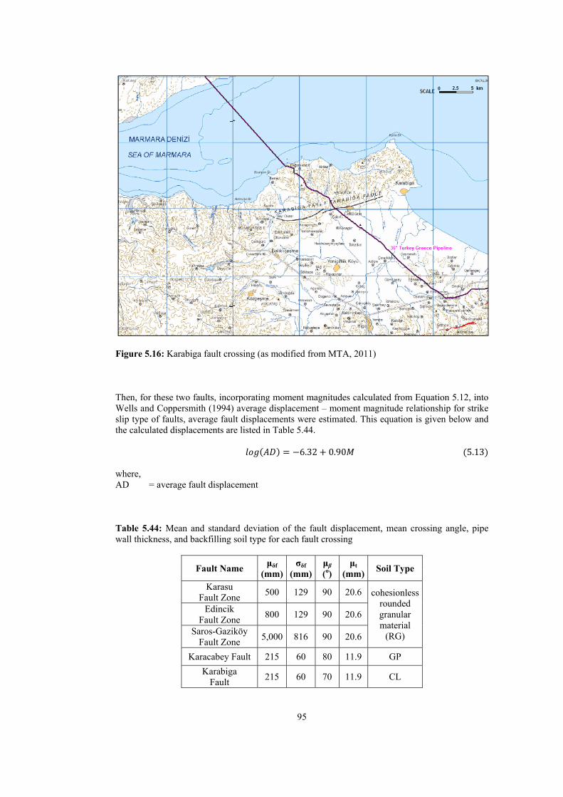
95

Figure 5.16: Karabiga fault crossing (as modified from MTA, 2011) Then, for these two faults, incorporating moment magnitudes calculated from Equation 5.12, into Wells and Coppersmith (1994) average displacement – moment magnitude relationship for strike slip type of faults, average fault displacements were estimated. This equation is given below and the calculated displacements are listed in Table 5.44. 6.32 0.90 5.13 where, AD = average fault displacement Table 5.44: Mean and standard deviation of the fault displacement, mean crossing angle, pipe wall thickness, and backfilling soil type for each fault crossing

Fault Name μδf

(mm)σδf

(mm)μβ

(o) μt

(mm)Soil Type

Karasu Fault Zone

500 129 90 20.6 cohesionless rounded granular material

(RG)

Edincik Fault Zone

800 129 90 20.6

Saros-Gaziköy Fault Zone

5,000 816 90 20.6

Karacabey Fault 215 60 80 11.9 GP

Karabiga Fault

215 60 70 11.9 CL

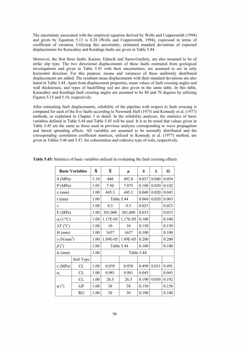
96

The uncertainty associated with the empirical equation derived by Wells and Coppersmith (1994) and given by Equation 5.13 is 0.28 (Wells and Coppersmith, 1994), expressed in terms of coefficient of variation. Utilizing this uncertainty, estimated standard deviations of expected displacements for Karacabey and Karabiga faults are given in Table 5.44. Moreover, the first three faults, Karasu, Edincik and Saros-Gaziköy, are also assumed to be of strike slip type. The two directional displacements of these faults estimated from geological investigations and given in Table 5.43 with their uncertainties, are assumed to act in only horizontal direction. For this purpose, means and variances of these uniformly distributed displacements are added. The resultant mean displacements with their standard deviations are also listed in Table 5.44. Apart from displacement properties, mean values of fault crossing angles and wall thicknesses, and types of backfilling soil are also given in the same table. In this table, Karacabey and Karabiga fault crossing angles are assumed to be 80 and 70 degrees by utilizing Figures 5.15 and 5.16, respectively. After estimating fault displacements, reliability of the pipeline with respect to fault crossing is computed for each of the five faults according to Newmark Hall (1975) and Kennedy et al. (1977) methods, as explained in Chapter 3 in detail. In the reliability analyses, the statistics of basic variables defined in Table 5.44 and Table 5.45 will be used. It is to be noted that values given in Table 5.45 are the same as those used in previous analyses corresponding to wave propagation and lateral spreading effects. All variables are assumed to be normally distributed and the corresponding correlation coefficient matrices, utilized in Kennedy et al. (1977) method, are given in Tables 5.46 and 5.47, for cohesionless and cohesive type of soils, respectively. Table 5.45: Statistics of basic variables utilized in evaluating the fault crossing effects


S (MPa) 1.10 448 492.8 0.037 0.040 0.054

P (MPa) 1.05 7.50 7.875 0.100 0.020 0.102

ri (mm) 1.00 445.3 445.3 0.040 0.020 0.045

t (mm) 1.00 Table 5.44 0.060 0.020 0.063

ν 1.00 0.3 0.3 0.023 0.023

E (MPa) 1.00 201,000 201,000 0.033 0.033

αt (1/oC) 1.00 1.17E-05 1.17E-05 0.100 0.100

ΔT (oC) 1.00 10 10 0.150 0.150

H (mm) 1.00 1657 1657 0.100 0.100

γ (N/mm3) 1.00 1.89E-05 1.89E-05 0.200 0.200

β (o) 1.00 Table 5.44 0.100 0.100

δf (mm) 1.00 Table 5.44

Soil Type

c (MPa) CL 1.00 0.038 0.038 0.490 0.031 0.491

αc CL 1.00 0.981 0.981 0.045 0.045

φ (o)

CL 1.00 26.5 26.5 0.190 0.030 0.192

GP 1.00 38 38 0.150 0.150

RG 1.00 30 30 0.100 0.100

97

Table 5.46: Correlation coefficient matrix, utilized in Kennedy et al. (1977) method for cohesionless type of soils

Sy ri t P ν E αt ΔT φ H γ Le

Sy 1.0 0.0 0.0 0.0 0.0 0.0 0.0 0.0 0.0 0.0 0.0 0.0

ri 0.0 1.0 0.0 0.0 0.0 0.0 0.0 0.0 0.0 0.0 0.0 -1.0

t 0.0 0.0 1.0 0.0 0.0 0.0 0.0 0.0 0.0 0.0 0.0 1.0

P 0.0 0.0 0.0 1.0 0.0 0.0 0.0 0.0 0.0 0.0 0.0 0.0

ν 0.0 0.0 0.0 0.0 1.0 0.0 0.0 0.0 0.0 0.0 0.0 0.0

E 0.0 0.0 0.0 0.0 0.0 1.0 0.0 0.0 0.0 0.0 0.0 1.0

αt 0.0 0.0 0.0 0.0 0.0 0.0 1.0 0.0 0.0 0.0 0.0 0.0

ΔT 0.0 0.0 0.0 0.0 0.0 0.0 0.0 1.0 0.0 0.0 0.0 0.0

φ 0.0 0.0 0.0 0.0 0.0 0.0 0.0 0.0 1.0 0.0 0.0 0.2

H 0.0 0.0 0.0 0.0 0.0 0.0 0.0 0.0 0.0 1.0 0.0 -1.0

γ 0.0 0.0 0.0 0.0 0.0 0.0 0.0 0.0 0.0 0.0 1.0 -1.0

Le 0.0 -1.0 1.0 0.0 0.0 1.0 0.0 0.0 0.2 -1.0 -1.0 1.0

Table 5.47: Correlation coefficient matrix, utilized in Kennedy et al. (1977) method for cohesive type of soils

Sy ri t P ν E αt ΔT φ H γ c αc Le

Sy 1.0 0.0 0.0 0.0 0.0 0.0 0.0 0.0 0.0 0.0 0.0 0.0 0.0 0.0

ri 0.0 1.0 0.0 0.0 0.0 0.0 0.0 0.0 0.0 0.0 0.0 0.0 0.0 0.0

t 0.0 0.0 1.0 0.0 0.0 0.0 0.0 0.0 0.0 0.0 0.0 0.0 0.0 1.0

P 0.0 0.0 0.0 1.0 0.0 0.0 0.0 0.0 0.0 0.0 0.0 0.0 0.0 0.0

ν 0.0 0.0 0.0 0.0 1.0 0.0 0.0 0.0 0.0 0.0 0.0 0.0 0.0 0.0

E 0.0 0.0 0.0 0.0 0.0 1.0 0.0 0.0 0.0 0.0 0.0 0.0 0.0 1.0

αt 0.0 0.0 0.0 0.0 0.0 0.0 1.0 0.0 0.0 0.0 0.0 0.0 0.0 0.0

ΔT 0.0 0.0 0.0 0.0 0.0 0.0 0.0 1.0 0.0 0.0 0.0 0.0 0.0 0.0

φ 0.0 0.0 0.0 0.0 0.0 0.0 0.0 0.0 1.0 0.0 0.0 0.0 0.0 0.0

H 0.0 0.0 0.0 0.0 0.0 0.0 0.0 0.0 0.0 1.0 0.0 0.0 0.0 -1.0

γ 0.0 0.0 0.0 0.0 0.0 0.0 0.0 0.0 0.0 0.0 1.0 0.0 0.0 -1.0

c 0.0 0.0 0.0 0.0 0.0 0.0 0.0 0.0 0.0 0.0 0.0 1.0 -1.0 -1.0

αc 0.0 0.0 0.0 0.0 0.0 0.0 0.0 0.0 0.0 0.0 0.0 -1.0 1.0 0.0

Le 0.0 0.0 1.0 0.0 0.0 1.0 0.0 0.0 0.0 -1.0 -1.0 -1.0 0.0 1.0

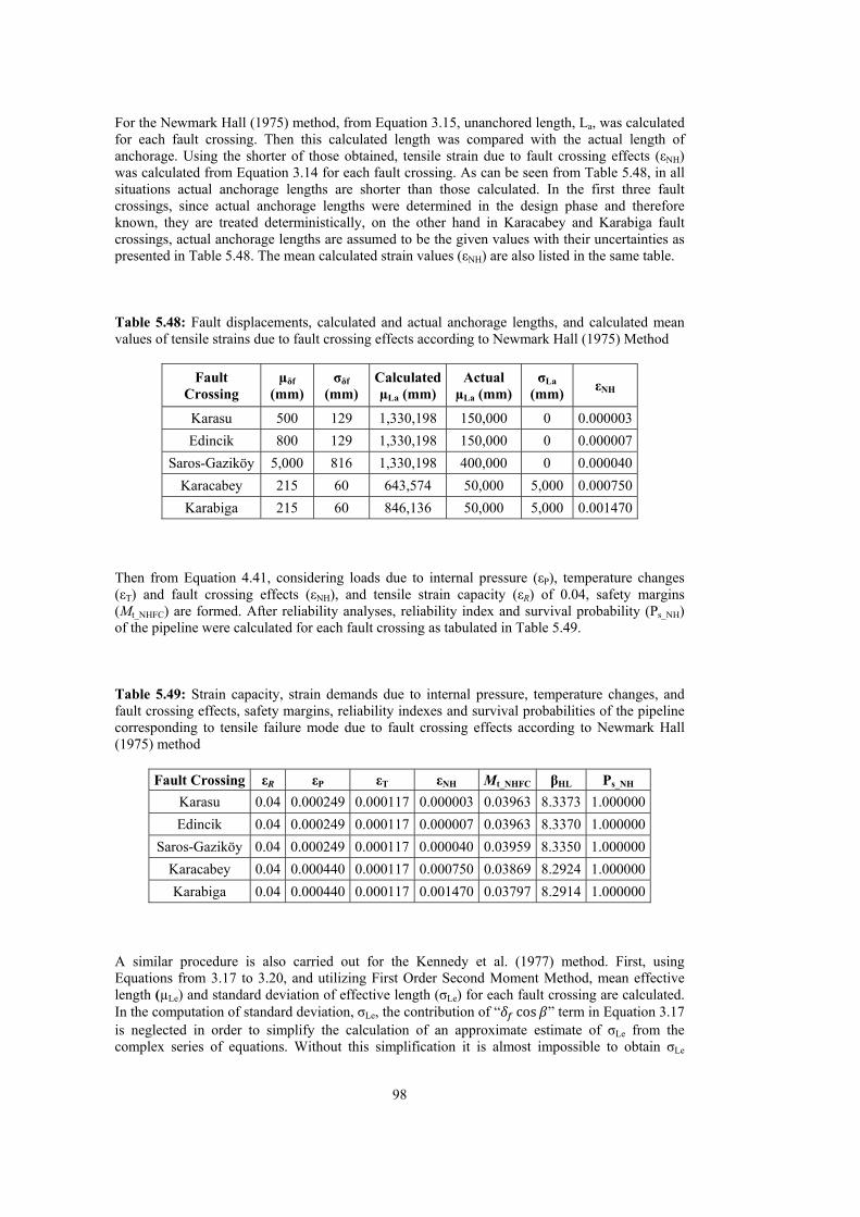
98

For the Newmark Hall (1975) method, from Equation 3.15, unanchored length, La, was calculated for each fault crossing. Then this calculated length was compared with the actual length of anchorage. Using the shorter of those obtained, tensile strain due to fault crossing effects (εNH) was calculated from Equation 3.14 for each fault crossing. As can be seen from Table 5.48, in all situations actual anchorage lengths are shorter than those calculated. In the first three fault crossings, since actual anchorage lengths were determined in the design phase and therefore known, they are treated deterministically, on the other hand in Karacabey and Karabiga fault crossings, actual anchorage lengths are assumed to be the given values with their uncertainties as presented in Table 5.48. The mean calculated strain values (εNH) are also listed in the same table. Table 5.48: Fault displacements, calculated and actual anchorage lengths, and calculated mean values of tensile strains due to fault crossing effects according to Newmark Hall (1975) Method

Fault Crossing

µδf (mm)

σδf (mm)

Calculated µLa (mm)

Actual µLa (mm)

σLa (mm)

εNH

Karasu 500 129 1,330,198 150,000 0 0.000003

Edincik 800 129 1,330,198 150,000 0 0.000007

Saros-Gaziköy 5,000 816 1,330,198 400,000 0 0.000040

Karacabey 215 60 643,574 50,000 5,000 0.000750

Karabiga 215 60 846,136 50,000 5,000 0.001470 Then from Equation 4.41, considering loads due to internal pressure (εP), temperature changes (εT) and fault crossing effects (εNH), and tensile strain capacity (εR) of 0.04, safety margins (Mt_NHFC) are formed. After reliability analyses, reliability index and survival probability (Ps_NH) of the pipeline were calculated for each fault crossing as tabulated in Table 5.49. Table 5.49: Strain capacity, strain demands due to internal pressure, temperature changes, and fault crossing effects, safety margins, reliability indexes and survival probabilities of the pipeline corresponding to tensile failure mode due to fault crossing effects according to Newmark Hall (1975) method

Fault Crossing εR εP εT εNH Mt_NHFC βHL Ps_NH

Karasu 0.04 0.000249 0.000117 0.000003 0.03963 8.3373 1.000000

Edincik 0.04 0.000249 0.000117 0.000007 0.03963 8.3370 1.000000

Saros-Gaziköy 0.04 0.000249 0.000117 0.000040 0.03959 8.3350 1.000000

Karacabey 0.04 0.000440 0.000117 0.000750 0.03869 8.2924 1.000000

Karabiga 0.04 0.000440 0.000117 0.001470 0.03797 8.2914 1.000000 A similar procedure is also carried out for the Kennedy et al. (1977) method. First, using Equations from 3.17 to 3.20, and utilizing First Order Second Moment Method, mean effective length (µLe) and standard deviation of effective length (σLe) for each fault crossing are calculated. In the computation of standard deviation, σLe, the contribution of “ cos ” term in Equation 3.17 is neglected in order to simplify the calculation of an approximate estimate of σLe from the complex series of equations. Without this simplification it is almost impossible to obtain σLe

99

analytically. This is justified since in most fault crossing, ≅ 90 and hence the expected value of cos 0. Then substituting mean effective length into the corresponding strain equation in Table 4.4, tensile strain due to fault crossing effects according to Kennedy et al. (1977) method, εK, was calculated for each fault crossing. The results are listed in Table 5.50. Table 5.50: Fault displacements, calculated means and standard deviations of effective lengths, and mean values of tensile strains due to fault crossing effects according to Kennedy et al. (1977) method

Fault Crossing µδf (mm) σδf (mm) µLe (mm) σLe (mm) εK

Karasu 500 129 128,393 43,653 0.00047

Edincik 800 129 170,221 50,436 0.00063

Saros-Gaziköy 5000 816 511,140 151,860 0.00188

Karacabey 215 60 112,975 25,272 0.00086

Karabiga 215 60 65,654 21,103 0.00243 Similar to Newmark Hall (1975) method, reliability analyses are carried out according to Kennedy et al. (1977) method. First, from Equation 4.41, considering operational loads (εP and εT), and loads due to fault crossing effects (εK), and tensile strain capacity (εR) of 0.04, safety margins (Mt_KFC) are formed. After reliability analyses, reliability index and survival probability (Ps_K) of the pipeline were calculated for each fault crossing according to Kennedy et al. (1977) method as listed in Table 5.51. Table 5.51: Strain capacity, strain demands due to internal pressure, temperature changes, and fault crossing effects, safety margins, reliability indexes and survival probabilities of the pipeline corresponding to tensile failure mode due to fault crossing effects according to Kennedy et al. (1977) method

Fault Crossing εR εP εT εK Mt_KFC βHL Ps_K

Karasu 0.04 0.00025 0.00012 0.00047 0.03916 7.3110 1.000000

Edincik 0.04 0.00025 0.00012 0.00063 0.03901 7.7052 1.000000

Saros-Gaziköy 0.04 0.00025 0.00012 0.00188 0.03775 3.4082 0.999673

Karacabey 0.04 0.00044 0.00012 0.00086 0.03858 8.3672 1.000000

Karabiga 0.04 0.00044 0.00012 0.00243 0.03702 1.9848 0.976417 In order to come up with a single value for the reliability of the pipeline corresponding to each fault crossing, this reliability is estimated based on the assumption that both methods are equally applicable to this case study. Thus, the average of the survival probabilities computed for each fault crossing according to both methods, given in Table 5.52 as Ps_FC, will be the survival probability of the pipeline with respect to tensile failure due to the effects of the corresponding fault crossing.

100

Table 5.52: Characteristic earthquake magnitudes of the faults, survival probabilities of the pipeline with respect to effects of these fault crossings according to Kennedy et al. (1977) and Newmark Hall (1975) methods, and average of these survival probabilities

Fault Crossing M Ps_K Ps_NH Ps_FC

Karasu 6.3 1.000000 1.000000 1.000000

Edincik 6.6 1.000000 1.000000 1.000000

Saros-Gaziköy 7.4 0.999673 1.000000 0.999837

Karacabey 6.3 1.000000 1.000000 1.000000

Karabiga 6.3 0.976417 1.000000 0.988208 The results have indicated that the pipeline has the highest risk at Karabiga fault crossing. This conclusion can be interpreted as reasonable because for this fault crossing there is not any countermeasure taken against seismic damage due to this effect. Taken into account that the backfilling soil is composed of cohesive soil, wall thickness has not been increased, and crossing angle is less than 90 degrees, such a result is not surprising. Additionally, although countermeasures were taken in order to mitigate against seismic damage to the pipeline throughout the Saros-Gaziköy fault crossing, corresponding reliability of the pipeline is not at high levels as a result of the significant fault displacement value.

5.3.3SurvivalProbabilityofthePipelineSubjectedtoDifferentEarthquakeEffects Survival probabilities for the Turkey-Greece Natural Gas Pipeline with respect to seismic wave propagation, liquefaction induced lateral spreading, liquefaction induced buoyancy and fault crossing effects have been computed in the previous subsections. In this section, these survival probabilities will be combined in order to estimate an overall survival probability of the pipeline taking into consideration all of these earthquake effects. In doing so it is to be noted that survival probabilities corresponding to reliability indexes which are computed above 7, are all assumed to be 1 in all cases. The survival probability of the pipeline due to all of these earthquake effects is estimated for two different levels of ground motion which are stated in Section 5.3.1. These are Functional Evaluation Earthquake (FEE) and Safety Evaluation Earthquake (SEE) ground motions. As mentioned before, the pipeline should be fully operational in case an earthquake in the first level, FEE, occurs, whereas only repairable damage is allowed in case the second level of earthquake, SEE, takes place. It is to be noted that FEE and SEE correspond to earthquakes having 10% and 2% probabilities of exceedence during an economic lifetime of 50 years, respectively. The survival probabilities for different earthquake effects are compiled as follows: Reliability of the pipeline against local buckling failure mode is adopted as the reliability of the pipeline subjected to wave propagation effects as stated in Section 5.3.1. Accordingly, conservative estimates of survival probabilities of the pipeline due to seismic wave propagation effects, Ps_WP, are given in Table 5.54 for both levels of earthquake.

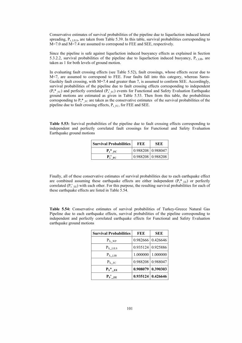
101

Conservative estimates of survival probabilities of the pipeline due to liquefaction induced lateral spreading, Ps_LILS, are taken from Table 5.39. In this table, survival probabilities corresponding to M=7.0 and M=7.4 are assumed to correspond to FEE and SEE, respectively. Since the pipeline is safe against liquefaction induced buoyancy effects as explained in Section 5.3.2.2, survival probabilities of the pipeline due to liquefaction induced buoyancy, Ps_LIB, are taken as 1 for both levels of ground motion. In evaluating fault crossing effects (see Table 5.52), fault crossings, whose effects occur due to M<7, are assumed to correspond to FEE. Four faults fall into this category, whereas Saros-Gaziköy fault crossing, with M=7.4 and greater than 7, is assumed to conform SEE. Accordingly, survival probabilities of the pipeline due to fault crossing effects corresponding to independent (Ps*_FC) and perfectly correlated (Ps'_FC) events for Functional and Safety Evaluation Earthquake ground motions are estimated as given in Table 5.53. Then from this table, the probabilities corresponding to Ps*_FC are taken as the conservative estimates of the survival probabilities of the pipeline due to fault crossing effects, Ps_FC, for FEE and SEE. Table 5.53: Survival probabilities of the pipeline due to fault crossing effects corresponding to independent and perfectly correlated fault crossings for Functional and Safety Evaluation Earthquake ground motions

Survival Probabilities FEE SEE

Ps*_FC 0.988208 0.988047

Ps'_FC 0.988208 0.988208 Finally, all of these conservative estimates of survival probabilities due to each earthquake effect are combined assuming these earthquake effects are either independent (Ps*_EE) or perfectly correlated (Ps'_EE) with each other. For this purpose, the resulting survival probabilities for each of these earthquake effects are listed in Table 5.54. Table 5.54: Conservative estimates of survival probabilities of Turkey-Greece Natural Gas Pipeline due to each earthquake effects, survival probabilities of the pipeline corresponding to independent and perfectly correlated earthquake effects for Functional and Safety Evaluation earthquake ground motions

Survival Probabilities FEE SEE

PS_WP 0.982666 0.426646

PS_LILS 0.935124 0.925886

PS_LIB 1.000000 1.000000

PS_FC 0.988208 0.988047

PS*_EE 0.908079 0.390303

PS'_EE 0.935124 0.426646

102

For the Functional Evaluation Earthquake: The survival probability of Turkey-Greece Natural Gas Pipeline subject to these earthquake effects is computed to be between 0.908079 and 0.935124. In other words, the failure probability of Turkey-Greece Natural Gas Pipeline due to earthquake induced effects is bounded between 0.064876 and 0.091921. For the Safety Evaluation Earthquake: The survival probability of Turkey-Greece Natural Gas Pipeline subject to these earthquake effects lies between 0.390303 and 0.426646. Stated in other words, the failure probability of Turkey-Greece Natural Gas Pipeline due to these earthquake effects is bounded between 0.573354 and 0.609697. These results show that failure probabilities of the pipeline against seismic threats are in the order of 8% for FEE and 59% for SEE. These high failure probabilities also indicate that the pipeline is under significant risk in the regions of high seismicity.

103

CHAPTER6

SUMMARYANDCONCLUSIONS

6.1Summary Buried continuous pipelines are generally used in the transportation of energy sources, such as natural gas, crude oil, etc. Therefore they are important structures which should sustain their functions properly, and without any interruption. These pipelines are separated from other types of pipelines because they are made of steel pipes, which are tough and ductile, and these pipes are connected to each other with strong arc welded joints. That is why these pipelines are called as continuous pipelines. Buried continuous pipelines are subjected to different kinds of loads. Load due to internal pressure is the main load for pipelines transporting natural gas. Together with this load, load resulting from temperature changes can be considered as the other operational load since it becomes effective when the pipeline is under operation. The other load effects, for example earth load and live load, may be taken into account at special situations such as road, railroad or river crossings, which are not considered in this study. In this study, only the above mentioned operating load effects are taken into consideration in addition to loads due to earthquake induced effects. There may be a number of earthquake effects that buried continuous pipelines are subjected to since they traverse a large geographical region and encounter a wide variety of soil conditions. These earthquake effects are split into two in terms of the state of soil deformations, which are transient and permanent. Seismic wave propagation affects the pipeline in the form of transient soil deformations, whereas liquefaction induced lateral spreading, liquefaction induced buoyancy and fault crossing effects to the pipeline take place due to permanent ground deformations (PGD). In this study, the effects of seismic wave propagation, liquefaction induced lateral spreading comprising longitudinal PGD and transverse PGD, liquefaction induced buoyancy, and fault crossing, evaluated by Newmark Hall (1975) and Kennedy et al. (1977) methods, are explained in detail. Reliability assessment of buried continuous pipelines subjected to these earthquake effects are the primary concern of this study. Accordingly, structural reliability of buried pipelines is also discussed. For this purpose, reliability methods, uncertainty modeling, failure modes of the pipeline, combination of these failure modes, limit state functions corresponding to these failure modes, and calculation of survival probabilities are all examined and explained in detail. In order to implement and illustrate the response and reliability analysis of buried continuous pipelines against operational and earthquake induced load effects, two case studies are presented. In the first study, reliability of an existing buried continuous natural gas pipeline (Hatay Natural Gas Pipeline) is assessed with respect to internal pressure only. In addition to this, safety factors corresponding to appropriate target reliability indexes are recommended as an alternative to the existing safety factors in ASME B31.8 code (2010).

104

In the other case study, reliability of another existing buried continuous natural gas pipeline (Turkey-Greece Natural Gas Pipeline) subjected to earthquake effects is assessed. In this case, the effects of seismic wave propagation, liquefaction induced lateral spreading, liquefaction induced buoyancy, and fault crossing to the pipeline are examined separately. For each effect and resulting failure modes, the reliability of the pipeline is assessed and lastly these earthquake effects are combined and the overall reliability of the pipeline subjected to all of these earthquake effects is estimated for the two levels of ground motions, namely: Functional Evaluation Earthquake and Safety Evaluation Earthquake ground motions.

6.2Conclusions The most significant conclusions as well as original contributions, recommendations derived from this study and discussion of the results are presented below: 1. Reliability assessment of buried continuous pipelines subjected to earthquake effects is the

first study carried out in this field in Turkey and may be considered as the most comprehensive one in the international literature on structural reliability.

2. Uncertainties utilized in reliability analyses are obtained from various sources because of the limited knowledge about the soil and pipeline properties in the case studies. However, mean values and coefficients of variation quantifying different sources of uncertainties have been tried to be consistent with the actual values as much as possible. For example, yield strength statistics of the Hatay pipeline is obtained from the manufacturer of the pipes installed in this project.

3. Reliability analyses considering only the internal pressure are carried out for each location classes according to ASME B31.8 code (2010) for the Hatay pipeline. Also safety factors corresponding to target reliability indexes are recommended for each of these location classes as an alternative to the existing safety factors. This work is also the first study in this field in Turkey.

4. Reliability analyses for the recommendations of new safety factors in the first case study are

carried out taking into account only the internal pressure without considering corrosion and the third party damages. On the other hand, ASME B31.8 code (2010) and target reliability indexes, which are calibrated in accordance with this code (Nessim et al., 2009), are determined in such a way that corrosion and third party damages are included. In the later studies, if these factors are also considered in the reliability analyses, more accurate results may be obtained. However, the results in the present study are reasonable especially when the first two location classes are examined. Because in these location classes, the likelihood of third party damages is low due to the low population density. Additionally, in all location classes, corrosion prevention methods, such as cathodic protection, 3 layers of polyethylene coating of the pipeline, etc., are applied to the pipeline. Accordingly, load due to the internal pressure can be adopted as the primary load in these location classes, and the contribution of the other effects mentioned above may be neglected.

5. Pipe costs constitute a significant portion of overall pipeline construction costs. Besides, pipe costs are directly proportional to wall thicknesses of pipes since the cost of the base metal (steel) of the pipe increases with tonnage. Thus, thinner wall thicknesses mean significant amount of cost savings in pipeline construction. Besides, costs of welding in the field decrease, since welding pipes having thinner wall thicknesses costs less. In the first case study, the safety factors corresponding to appropriate reliability indexes are computed as

105

consistently higher than the code specified safety factors. Therefore existing safety factors could be replaced with the recommended safety factors in order to attain a uniform level of safety and prevent the monetary losses resulting from overdesign since the wall thicknesses computed from using recommended safety factors are less than those computed based on existing safety factors specified in ASME B31.8 (2010).

6. Except landslide and settlement, nearly all earthquake effects to buried continuous pipelines

are examined and evaluated in assessing safety in terms of reliability. Seismic wave propagation, liquefaction induced lateral spreading, liquefaction induced buoyancy, and fault crossing effects to buried continuous pipelines are explained and illustrated in a case study in detail. Such a comprehensive reliability study based on real life data has been carried out for the first time in Turkey as well as internationally.

7. The results of the wave propagation effects to buried continuous pipelines indicate that the

pipeline is safe in the tensile failure mode having a resisting strain capacity of 0.04. However, the safety evaluation is different for local buckling failure mode. This type of failure becomes more likely if the pipeline is buried in cohesive soils in high seismicity regions. The failure probabilities computed were quite high confirming this statement in such locations. If wall thickness of the pipeline is increased and the backfilling soil is selected of the cohesionless type instead of local cohesive soil, the seismic wave propagation effects can be reduced in these most hazardous regions.

8. Liquefaction induced lateral spreading may create a risk to pipelines when they traverse

liquefaction susceptible regions. In the second case study such a region is evaluated in terms of its effects to an existing buried continuous pipeline. Lateral spreading may be of two types with respect to the orientation of the pipeline, namely: Longitudinal PGD and transverse PGD. Longitudinal PGD effects are more dangerous with the increase of the length of PGD zone, whereas for the transverse PGD effects, the opposite of this is valid. When the results of lateral spreading effects to the pipeline is examined, longer sections of the pipeline are found more susceptible to adverse effects of longitudinal PGD than transverse PGD. Moreover, the pipeline is safe against transverse PGD effects throughout all sections of the pipeline. However, since the exact direction of PGD is not known, treating these PGD effects equally likely, and taking the average of the survival probabilities of the pipeline due to each effect, is considered as a reasonable approach for this case. Because of the above mentioned reasons, decreasing the lengths of the pipe sections (assumed as four in the case study) and as a result, increasing number of sections, will not change the results significantly. Therefore, the lengths and number of sections selected in the second case study in the lateral spreading zone are reasonable.

9. Liquefaction induced buoyancy generally can be treated as a serviceability limit state for buried continuous pipelines instead of ultimate limit state. The case study also confirms this statement since this effect does not create any risk to the pipeline in terms of ultimate limit state. However, it is calculated that for a critical buoyancy length of 61 m, the pipeline may seriously be harmed due to this type of earthquake effect.

10. Fault crossings are generally considered as the most significant earthquake effect to buried

continuous pipelines in literature. Thus, mitigation countermeasures against this effect deserve the most attention in pipeline construction. In the second case study, involving the reliability assessment of Turkey-Greece Natural Gas Pipeline, when the pipeline is examined in terms of its response to this effect, it is observed that at the crossings where such countermeasures are taken by BOTAŞ, the pipeline shows good performances, whereas at the crossing of the Karabiga fault, which was not taken into account in the design and construction phases, it displays a more critical response.

11. Two methods, Newmark Hall (1975) and Kennedy et al. (1977), are explained and utilized in

the reliability analyses of buried continuous pipelines subjected to fault crossing effects.

106

Since these methods are applicable to strike slip type of faults and to the pipelines in tension, then the faults, which exhibit two directional behavior in the route of the pipeline considered, are assumed to be of strike slip type. With the improvement of the analytical methods, applicable to all type of faults, more accurate results may be obtained. However, the results in this study are reasonable in terms of the direction of resulting strains, since the normal and oblique (in this study it refers to the faults exhibiting both strike-slip and normal type of behavior at the same time) faults, which cause tensile strains in the pipeline, are assumed to be of strike slip.

12. Reliability analyses have been carried out by using the following algorithms: AFOSM code

written by the author in Mathcad program, constrained optimization algorithm described by Thoft-Christensen and Baker (1982) in Mathcad, Low and Tang (2004) method using MS Excel solver. All of these algorithms yield to the same results when limit state functions are formed from simple equations, such as the one corresponding to the evaluation of internal pressure as the only load effect. However, since limit state functions corresponding to earthquake loads are composed of complex equations, only the code written in Mathcad program by the author can be utilized. The other two algorithms were not applicable to such complex equations.

13. All of the earthquake effects are considered together with the operating loads, which are

loads due to internal pressure and temperature changes. Lastly, survival probabilities of the pipeline subjected to all these effects are combined in such a way that different earthquake effects are assumed either to be mutually independent or perfectly correlated with each other. In this way bounds were established for the true survival probability for both of the ground motion levels, which are Functional Evaluation Earthquake and Safety Evaluation Earthquake ground motions. The results have indicated that the Turkey-Greece Natural Gas Pipeline is under significant degree of risk under both levels of ground motion.

14. These undesirable performances may be reduced by taking countermeasures in the design and

construction phases. As mentioned before, increasing wall thicknesses, improving the pipe material strength, avoiding cohesive types of backfilling soil, and also changing the route of the pipeline to avoid fault crossings, liquefaction susceptible and/or high seismicity regions, are the recommended countermeasures in order to enhance the reliability of the buried continuous pipelines subjected to earthquake effects.

15. This study also enables the assessment of the insurance premiums for buried continuous

pipelines against earthquake induced effects. In other words, reliability based safety assessment of the pipelines subjected to earthquake effects is a significant step for the realistic estimation of the insurance premiums of these pipelines against seismic hazards. This study can be extended to serve for this purpose.

16. It is hoped that the work, carried out in relation with this thesis, initiates and encourages the

research work in the reliability based design of buried continuous pipelines in Turkey. In future studies, reliability based safety factors corresponding to selected reliability indexes may be developed for the design of pipelines with respect to hazards resulting from fault crossings, liquefaction susceptible regions and/or high seismicity regions, where the route of the pipeline cannot be altered, and such hazards cannot be avoided. The present study can also be extended to include the other load effects resulting from road, railroad and river crossings, and pipe bends. Furthermore, a Turkish code for the design of buried continuous pipelines taking into consideration the specific conditions of Turkey, can be drafted.

107

REFERENCES

Ahammed, M. and Melchers, R.E., 1997, “Probabilistic Analysis of Underground Pipelines Subject to Combined Stress and Corrosion”, Engineering Structures, Vol. 19, No:12, pp. 998-994, Elsevier. Ahammed, M. 1998, “Probabilistic Estimation of Remaining Life of a Pipeline in the Presence of Active Corrosion Defects”, International Journal of Pressure Vessels and Piping 75, pp. 321–329, Elsevier. American Lifelines Alliance, ALA, July 2001 (with addenda through February 2005), “Guidelines for the Design of Buried Steel Pipe”, A Report by Public-private Partnership between American Society of Civil Engineers (ASCE) & Federal Emergency Management Agency (FEMA). American Lifelines Alliance, ALA, March 2005, “Seismic Guidelines for Water Pipelines”, A Report by Public-private Partnership between Federal Emergency Management Agency (FEMA) and National Institute of Building Sciences (NIBS). American Petroleum Institute, API, August 1996, “Movement of In-Service Pipelines”, API Recommended Practice 1117, Second Edition, USA. American Petroleum Institute, API, 2007, “Specification for Line Pipe”, API Specification 5L, 44th Edition, USA. American Society of Civil Engineers, ASCE, 1984, “Guidelines for the Seismic Design of Oil and Gas Pipeline Systems”, Committee on Gas and Liquid Fuel Lifelines. American Society of Mechanical Engineers, ASME, 2010, “B31.8 Gas Transmission and Distribution Piping Systems”, ASME Code for Pressure Piping. Amirat, A., Mohamed-Chateauneuf, A., Chaoui, K., 2006, “Reliability Assessment of Underground Pipelines under the Combined Effect of Active Corrosion and Residual Stress”, International Journal of Pressure Vessels and Piping 83, Elsevier, pp. 107–117. Ang, A. H.S and Tang, W.H., 1984, “Probability Concepts in Engineering Planning and Design”, Volume II, John Wiley and Sons Inc., New York. Bai, Y. and Mork, K. J., 1994, "Probabilistic Assessment of Dented and Corroded Pipeline", International Conference on Offshore and Polar Engineering, Osaka, Japan.

108

Bai, Y., 2001, "Chapter 14 Remaining Strength of Corroded Pipes", Pipelines and Risers, Elsevier Ocean Engineering Series, Vol. 3, pp. 229-255. Bai, Y., 2003, "Chapter 26 Reliability-Based Design and Code Calibration", Marine Structural Design, Elsevier Science, Oxford, pp. 463-480. Bardet, J. P., Tobita, T., and Mace, N., Hu, J., 2002, “Regional Modeling of Liquefaction Induced Ground Deformation”, Earthquake Spectra, EERI, Vol. 18. Bartlett, S.F. and Youd, T.L., 1992, “Empirical Analysis of Horizontal Ground Displacement Generated by Liquefaction-Induced Lateral Spreads”, Technical Report NCEER-92-0021, Multidisciplinary Center for Earthquake Engineering Research, Buffalo, NY. Bea, R., Xu, T., 16 June 2000, “Risk Assessment and Management (RAM) Based Guidelines for Requalification of Marine Pipelines”, RAM PIPE REQUAL, Pipeline Requalification Guidelines Project Report 4. BOTAŞ Specifications, 10 January 2000, "Ditch Dimensions and Backfilling", Transmission/Branch Lines Typical Drawings, Dwg No: BOT-TYP-PL-0015. BOTAŞ, 2003, "Route Inspection and Investigation Report", Turkey Greece Pipeline System Engineering Works Project, Document Number: RC426.RA.100.C040.1007 BOTAŞ, 2009, "Technical Specifications", Hatay Natural Gas Pipeline Project Procurement Documents, Ankara. Caleyo, F., Gonzales, J.L., Hallen, J.M., 2002, “A Study on the Reliability Assessment Methodology for Pipelines with Active Corrosion Defects”, International Journal of Pressure Vessels and Piping 79, Elsevier, pp. 77–86. Chen, Q. C., Fuglem, M., Stephens, M. J., and Zhou, J., 2001, “Reliability- Based Pipeline Design for Mechanical Damage,” 13th Biennial Joint Technical Meeting on Pipeline Research, Apr. 3–May 4. Cornell, C. A., 1969, “A Probability-based Structural Code.”, J. Amer. Conc. Inst., 66(12): 974-985. Duncan, J. M., 2000, “Factors of Safety and Reliability in Geotechnical Engineering”, Journal of Geotechnical and Geoenvironmental Engineering, ASCE, Vol. 126, No. 4, pp. 307-316. Ellingwood, B.R., Galambos, T.V., MacGregor, J.G. and Cornell, C.A., 1980, “Development of a Probability Based Load Criterion for American National Standards A58”, NPS Special Publication 577, 1980.

109

GSDMA, November 2007, “Guidelines for Seismic Design of Buried Pipelines”, National Information Center of Earthquake Engineering, Indian Institute of Technology Kanpur, Kanpur (India). Gutierrez, M., Duncan, J. M., Woods, C., and Eddy, M., 2003, “Development of a Simplified Reliability-Based Method for Liquefaction Evaluation”, Final Technical Report, Virginia Polytechnic Institute and State Institute, Blacksburg, Virginia. Hall, W. and Newmark, N., 1977, “Seismic Design Criteria for Pipelines and Facilities”, in Current State of Knowledge of Lifeline Earthquake Engineering, American Society of Civil Engineers, New York, pp. 18–34. Hamada, M., Yasuda, S., Isoyama, R., and Emoto, K., 1986, “Study on Liquefaction Induced Permanent Ground Displacements”, Association for the Development of Earthquake Prediction, Japan. Hansen, J.B., 1961, “The Ultimate Resistance of Rigid Piles Against Transversal Forces”, Bulletin 12, Danish Geotechnical Institute, Copenhagen, Denmark. Hasofer, A. A. and Lind, A. M., 1974, “An Exact and Invariant Second-Moment Code Format”, Journal of the Engineering Mechanics Division, ASCE, Vol. 100, pp. 111-121. Kalkan, E., Gülkan, P., Yilmaz, N., and Çelebi, M., August 2009, “Reassessment of Probabilistic Seismic Hazard in the Marmara Region”, Bulletin of the Seismological Society of America, v. 99, no. 4, p. 2127-2146. Kennedy, R.P., Chow, A.W., and Williamson, R.A., 1977, “Fault Movement Effects on Buried Oil Pipeline”, J. Transport. Eng. Div., 103 (TE5), pp. 617–633. Liao, S. S., Veneziano, D., and Whitman, R. V., 1988, “Regression Models for Evaluating Liquefaction Probability”, Journal of Geotechnical Engineering, vol. 114, no. 4, April. Loehr, J.E., Finley, C.A., and Huaco, D.R., 2005, “Final Report for RI03-030: Procedures for Design of Earth Slopes Using LRFD”, Civil & Environmental Engineering University of Missouri – Columbia, Missouri. McCaffrey, M.A. and O’Rourke, T.D., June 1983, “Buried Pipeline Response to Reverse Faulting during the 1971 San Fernando Earthquake,” Earthquake Behavior and Safety of Oil and Gas Storage Facilities, Buried Pipelines and Equipment, PVP-77, American Society of Mechanical Engineers, New York, pp. 151–159. Michalopoulos, E., and Babka, S., 2000, “Evaluation Of Pipeline Design Factors”, Task Report, Hartford.

110

MTA, 2011, “1:250,000 Scale Active Fault Map Series of Turkey”, General Directorate of Mineral Research and Exploration. Nessim, M. A., Zhou, W., Zhou, J., Rothwell, B., and McLamb, M., 2009, “Target Reliability Levels for Design and Assessment of Onshore Natural Gas Pipelines”, ASME Journal of Pressure Vessel Technology, Vol. 131, No. 12, DOI:10.1115/1.3110017. Newmark, N.M., 1967, “Problems in Wave Propagation in Soil and Rocks”, in Proceedings of the International Symposium on Wave Propagation and Dynamic Properties of Earth Materials, University of New Mexico Press, Albuquerque, pp. 7–26. Newmark, N. M., and Hall W. J., 1975, “Pipeline Design to Resist Large Fault Displacement”, Proceedings of the U.S. National Conference on Earthquake Engineering, Ann Arbor, Michigan, EERI, pp. 416–425. NEHRP, February 1997, “Recommended Provisions for Seismic Regulations for New Buildings and Other Structures”, Part 1 - Provisions, Federal Emergency Management Agency. O’Rourke, M.J., Liu, X.J., and Flores-Berrones, R. (1995). “Steel Pipe Wrinkling due to Longitudinal Permanent Ground Deformation”, J. Transport. Eng., 121, pp. 443–451. O’Rourke, M.J. and Liu, X., 1999, “Response of Buried Pipelines Subject to Earthquake Effects”, Monograph Number 3, Multidisciplinary Center for Earthquake Engineering Research, MCEER, Buffalo, New York. O’Rourke, M.J., 2003, “Buried Pipelines”, Chapter 23 in Earthquake Engineering Handbook, Edited by Chen, W., Scawthorn, C., CRC Press. Pipeline Research Council International, PRCI, October 2004, “Guidelines for the Seismic Design and Assessment of Natural Gas and Liquid Hydrocarbon Pipelines, Pipeline Design, Construction and Operations”, Edited by Honegger, D. G., and Nyman D. J., Technical Committee of PRCI Inc. Ramberg, W., and Osgood, W R., July 1943, “Description of Stress-Strain Curves by Three Parameters”, Technical Notes: National Advisory Committee for Aeronautics, Washington. Rockwell, T., Barka, A., Dawson, T., Akyüz, S. ve Thorup K., 2001, “Paleoseismology of the Gaziköy Segment of the North Anatolian Fault, Northwestern Turkey: Comparison of the Historical and Paleoseismic Records, Implications of Regional Seismic Hazard and Models of Earthquake Recurrence”, Journal of Seismology, 5, pp.433-448. Şaroğlu F., Emre Ö. ve Kuşçu İ., 1992, Türkiye Diri Fay Haritası, 1:2,000,000 ölçekli, Maden Tetkik ve Arama Genel Müdürlüğü, Ankara.

111

Seed, H. B. and Idriss, I. M., 1982, “Ground Motions and Soil Liquefaction during Earthquakes”, Earthquake Engineering Research Institute, University of California, Berkeley, 134 pp. Thoft-Christensen, P. and Baker, M. J., 1982, “Structural Reliability Theory and Its Applications”, Springer Verlag, Berlin. TSC, 2007, “Specification for Buildings to be built in Seismic Zones”, Ministry of Public Works and Settlement Government of Republic of Turkey, Ankara. U.S. Army Corps of Engineers, 1997, “Engineering and Design, Introduction to Probability and Reliability Methods for Use in Geotechnical Engineering”, Engr. Tech. Letter No. 1110-2-547, Department of the Army, Washington. Wells, D.L. and K.J. Coppersmith, 1994, “New Empirical Relationships among Magnitude, Rupture Length, Rupture Width, Rupture Area, and Surface Displacement”, Bull. Seismol. Soc. Am., 84, 974–1002. Yeh, G., 1974, “Seismic Analysis of Slender Buried Beams”, Bull. Seismol. Soc. Am., 64, 1551–1562. Yücemen, M.S., 2006, “Unpublished Lecture Notes of CE 589 Structural Reliability”, Department of Civil Engineering, METU, Ankara. Zhou, W., Nessim, M. A., Zhou, J., February 15-16, 2006, “Application of Reliability-based Design and Assessment to Natural Gas Pipelines”, The Pipeline Pigging and Integrity Management Conference, Houston, Texas.

113

APPENDIXA

SOILINDUCEDFORCES

A.1AxialSoilForce The maximum axial soil force per unit length of pipe that can be transmitted to the pipe is (ALA, 2001): 1 2 tan . 1

where: D = outside diameter of pipe c = soil cohesion representative of the soil backfill αc = adhesion factor (curve fit to plots of recommended values in Figure A.1)

= 0.618 0.123 . . where c is in kPa/100

H = depth to pipe centerline γ’ = effective unit weight of soil Ko = coefficient of pressure at rest = 1 sin ′ φ’ = internal friction angle of soil δ’ = interface angle of friction for pipe and soil = ′ f = coating dependent factor relating the internal friction angle of the soil to the friction

angle at the soil-pipe interface (see Table A.1) Table A.1: Friction factor, f, for various external coatings

Pipe Coating f Concrete 1.0 Coal Tar 0.9

Rough Steel 0.8 Smooth Steel 0.7

Fusion Bonded Epoxy 0.6 Polyethylene 0.6

114

Figure A.1: Plotted values for the adhesion factor, αc

A.2LateralSoilForce The maximum lateral soil force per unit length of pipe that can be transmitted to the pipe is (ALA, 2001): . 2 where, Nch = horizontal bearing capacity factor for clay (0 for c = 0)

= 9 where the parameters are in Table A.2

Nqh = horizontal bearing capacity factor (0 for φ = 0o) = where the parameters are in Table A.2 Table A.2: Closed form fit parameters to published empirical (plotted) results in Figure A.2

Factor φ x a b c d e

Nch 0 H/D 6.752 0.065 -11.063 7.119 -

Nqh 20 H/D 2.399 0.439 -0.030 1.059E-03 -1.754E-05

Nqh 25 H/D 3.332 0.839 -0.090 5.606E-03 -1.319E-04

Nqh 30 H/D 4.565 1.234 -0.089 4.275E-03 -9.159E-05

Nqh 35 H/D 6.816 2.019 -0.146 7.651E-03 -1.683E-04

Nqh 40 H/D 10.959 1.783 0.045 -5.425E-03 -1.153E-04

Nqh 45 H/D 17.658 3.309 0.048 -6.443E-03 -1.299E-04Note: Nqh can be interpolated for intermediate values of φ between 20o and 45o

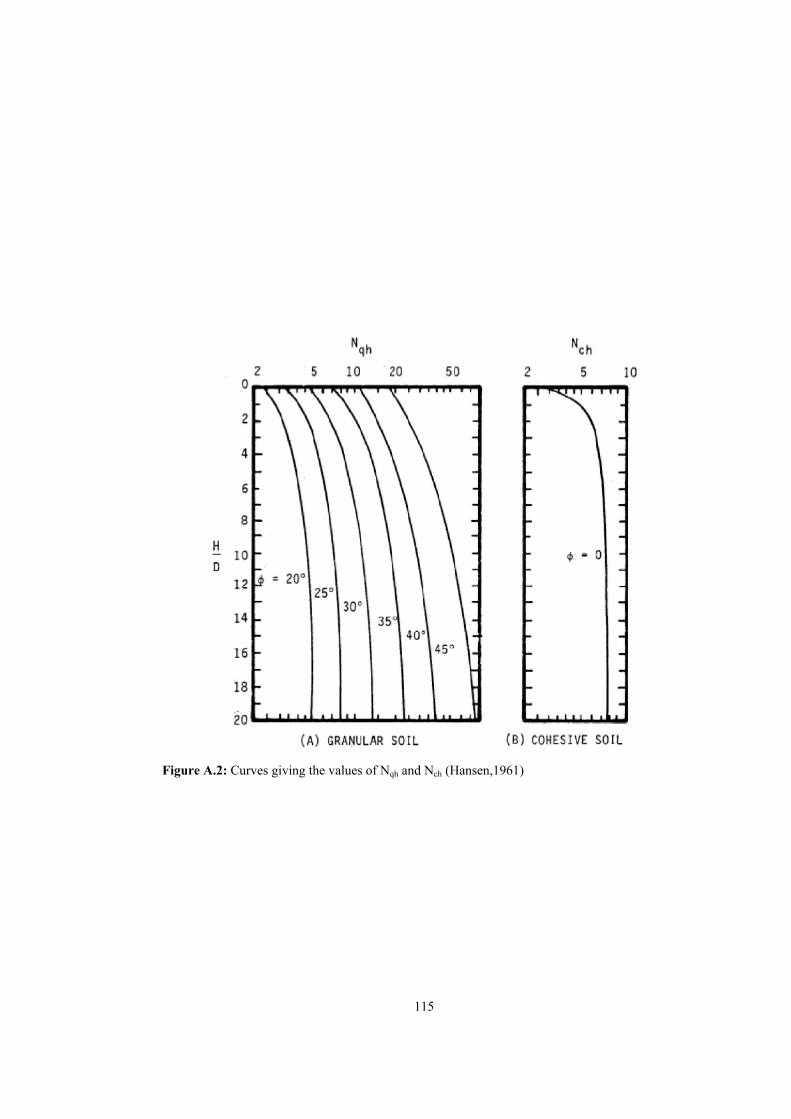
115

Figure A.2: Curves giving the values of Nqh and Nch (Hansen,1961)

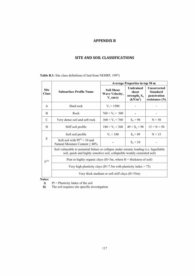
117

APPENDIXB

SITEANDSOILCLASSIFICATIONS

Table B.1: Site class definitions (Cited from NEHRP, 1997)

Site Class

Subsurface Profile Name

Average Properties in top 30 m

Soil Shear Wave Velocity,

Vs (m/s)

Undrained shear

strength, Su (kN/m2)

Uncorrected Standard

penetration resistance (N)

A Hard rock Vs > 1500 - -

B Rock 760 < Vs < 500 - -

C Very dense soil and soft rock 360 < Vs < 760 Su > 98 N > 50

D Stiff soil profile 180 < Vs < 360 49 < Su < 98 15 < N < 50

E Soft soil profile Vs < 180 Su < 49 N < 15

Soft soil with PI(i) > 10 and Natural Moisture Content ≥ 40%

- Su < 24 -

F(ii)

Soil vulnerable to potential failure or collapse under seismic loading (i.e. liquefiable soil, quick and highly sensitive soil, collapsible weakly cemented soil)

Peat or highly organic clays (H>3m, where H = thickness of soil)

Very high plasticity clays (H>7.5m with plasticity index > 75)

Very thick medium or soft stiff clays (H>35m)

Notes: i) PI = Plasticity Index of the soil

ii) The soil requires site specific investigation

118

Table B.2: Unified soil classification system

Soil Classification

Explanation

GW Well-graded gravels, gravel-sand mixtures, little or no fines GP Poorly-graded gravels, gravel-sand mixtures, little or no fines GM Silty gravels, gravel-sand-silt mixtures GC Clayey gravels, gravel-sand-day mixtures SW Well-graded sands, gravelly sands, little or no fines SP Poorly graded sands, gravelly sands, little or no fines SM Silty sands, sand-silt mixtures SC Clayey sands, sand-clay mixtures

ML Inorganic silts and very fine sands, rock flour, silty of clayey fine sands

or clayey silts with slight plasticity

CL Inorganic clays of low to medium plasticity, gravelly clays, sandy

clays, silty clays, lean clays OL Organic silts and organic silty clays of low plasticity

MH Inorganic silts, micaceous or diatomaceous fine sandy or silty soils,

elastic silts CH Inorganic clays of high plasticity, fat clays OH Organic clays of medium to high plasticity, organic silts PT Peat and other highly organic soils

RELIABILITY BASED SAFETY ASSESSMENT OF BURIED …etd.lib.metu.edu.tr/upload/12615423/index.pdf ·...

Documents

Transcript of RELIABILITY BASED SAFETY ASSESSMENT OF BURIED …etd.lib.metu.edu.tr/upload/12615423/index.pdf ·...