1

Reliability and Performance Modeling and Analysis

for Grid Computing

Yuan-Shun Dai 1,2, Jack Dongarra 1,3,4

1 Department of Electrical Engineering and Computer Science, University of Tennessee, Knoxville

2 Department of Industrial and Information Engineering,

University of Tennessee, Knoxville

3 Oak Ridge National Laboratory

4 University of Manchester

Abstract

Grid computing is a newly developed technology for complex systems with large-scale

resource sharing, wide-area communication, and multi-institutional collaboration. It is hard to

analyze and model the Grid reliability because of its largeness, complexity and stiffness.

Therefore, this chapter introduces the Grid computing technology, presents different types of

failures in grid system, models the grid reliability with star structure and tree structure, and

finally studies optimization problems for grid task partitioning and allocation. The chapter

then presents models for star-topology considering data dependence and tree-structure

considering failure correlation. Evaluation tools and algorithms are developed, evolved from

Universal generating function and Graph Theory. Then, the failure correlation and data

dependence are considered in the model. Numerical examples are illustrated to show the

modeling and analysis.

Keywords: Reliability, Performance, Grid computing, Modeling, Graph theory, Bayesian

approach.

2

1. Introduction Grid computing (Foster & Kesselman, 2003) is a newly developed technology for complex

systems with large-scale resource sharing, wide-area communication, and multi-institutional

collaboration etc, see e.g. Kumar (2000), Das et al. (2001), Foster et al. (2001, 2002) and

Berman et al. (2003). Many experts believe that the grid technologies will offer a second

chance to fulfill the promises of the Internet.

The real and specific problem that underlies the Grid concept is coordinated resource

sharing and problem solving in dynamic, multi-institutional virtual organizations (Foster et

al., 2001). The sharing that we are concerned with is not primarily file exchange but rather

direct access to computers, software, data, and other resources. This is required by a range of

collaborative problem-solving and resource-brokering strategies emerging in industry, science,

and engineering. This sharing is highly controlled by the resource management system

(Livny & Raman, 1998), with resource providers and consumers defining what is shared, who

is allowed to share, and the conditions under which the sharing occurs.

Recently, the Open Grid Service Architecture (Foster et al., 2002) enables the integration

of services and resources across distributed, heterogeneous, dynamic, virtual organizations. A

grid service is desired to complete a set of programs under the circumstances of grid

computing. The programs may require using remote resources that are distributed. However,

the programs initially do not know the site information of those remote resources in such a

large-scale computing environment, so the resource management system (the brain of the grid)

plays an important role in managing the pool of shared resources, in matching the programs

to their requested resources, and in controlling them to reach and use the resources through

wide-area network.

The structure and functions of the resource management system (RMS) in the grid have

been introduced in details by Livny & Raman (1998), Cao et al. (2002), Krauter et al. (2002)

and Nabrzyski et al. (2003). Briefly stated, the programs in a grid service send their requests

for resources to the RMS. The RMS adds these requests into the request queue (Livny &

Raman, 1998). Then, the requests are waiting in the queue for the matching service of the

RMS for a period of time (called waiting time), see e.g. Abramson et al. (2002). In the

matching service, the RMS matches the requests to the shared resources in the grid (Ding et

3

al., 2002) and then builds the connection between the programs and their required resources.

Thereafter, the programs can obtain access to the remote resources and exchange information

with them through the channels. The grid security mechanism then operates to control the

resource access through the Certification, Authorization and Authentication, which constitute

various logical connections that causes dynamicity in the network topology.

Although the developmental tools and infrastructures for the grid have been widely

studied (Foster & Kesselman, 2003), grid reliability analysis and evaluation are not easy

because of its complexity, largeness and stiffness. The gird computing contains different

types of failures that can make a service unreliable, such as blocking failures, time-out

failures, matching failures, network failures, program failures and resource failures. This

chapter thoroughly analyzes these failures.

Usually the grid performance measure is defined as the task execution time (service time).

This index can be significantly improved by using the RMS that divides a task into a set of

subtasks which can be executed in parallel by multiple online resources. Many complicated

and time-consuming tasks that could not be implemented before are working well under the

grid environment now.

It is observed in many grid projects that the service time experienced by the users is a

random variable. Finding the distribution of this variable is important for evaluating the grid

performance and improving the RMS functioning. The service time is affected by many

factors. First, various available resources usually have different task processing speeds

online. Thus, the task execution time can vary depending on which resource is assigned to

execute the task/subtasks. Second, some resources can fail when running the subtasks, so the

execution time is also affected by the resource reliability. Similarly, the communication links

in grid service can be disconnected during the data transmission. Thus, the communication

reliability influences the service time as well as data transmission speed through the

communication channels. Moreover, the service requested by a user may be delayed due to

the queue of earlier requests submitted from others. Finally, the data dependence imposes

constraints on the sequence of the subtasks' execution, which has significant influence on the

service time.

This chapter first introduces the grid computing system and service, and analyzes various

4

failures in grid system. Both reliability and performance are analyzed in accordance with the

performability concept. Then the chapter presents models for star- and tree-topology grids

respectively. The reliability and performance evaluation tools and algorithms are developed

based on the universal generating function, graph theory, and Bayesian approach. Both failure

correlation and data dependence are considered in the models. 2. Grid Service Reliability and Performance

2.1. Description of the grid computing

Today, the Grid computing systems are large and complex, such as the IP-Grid

(Indiana-Purdue Grid) that is a statewide grid (http://www.ip-grid.org/). IP-Grid is also a part

of the TeraGrid that is a nationwide grid in the USA (http://www.teragrid.org/). The largeness

and complexity of the grid challenge the existing models and tools to analyze, evaluate,

predict and optimize the reliability and performance of grid systems. The global grid system

is generally depicted by the Fig. 1. Various organizations (Foster et al., 2001), integrate/share

their resources on the global grid. Any program running on the grid can use those resources if

it can be successfully connected to them and is authorized to access them. The sites that

contain the resources or run the programs are linked by the global network as shown in the

left part of Fig. 1.

5

GridResource

Management

Large-Scale Grid

P1,…R1,… P,…

R,…

P,…

SharedResources

AccessControl

Global RM

Inter-requestRM

Requestqueue

ApplicationPrograms

Resourceoffers

Resourcerequests

Matches

Matches

clai

min

gResourcedescriptions

Resourcesites

Res

ourc

e ac

cess

ProgramLayer

RequestLayer

ManagementLayer

ResourceLayer

NetworkLayer

P=ProgramR=ResourceRM=Resource ManagementRMS=Resource Management System

Notations:

Five LayersNetwork

Fig. 1. Grid Computing System

The distribution of the service tasks/subtasks among the remote resources are controlled

by the Resource Management System (RMS) that is the “brain” of the grid computing, see

e.g. Livny & Raman (1998). The RMS has five layers in general, as shown in Fig. 1: program

layer, request layer, management layer, network layer and resource layer.

1) Program layer: The program layer represents the programs of the customer’s applications. The programs describe their required resources and constraint requirements (such as deadline, budget, function etc). These resource descriptions are translated to the resource requests and sent to the next request layer.

2) Request layer: The request layer provides the abstraction of “program requirements” as a queue of resource requests. The primary goals of this layer are to maintain this queue in a persistent and fault-tolerant manner and to interact with the next management layer by injecting resource requests for matching, claiming matched resources of the requests.

3) Management layer: The management layer may be thought of as the global resource allocation layer. It has the function of automatically detecting new resources, monitoring the resource pool, removing failed/unavailable resources, and most importantly matching the resource requests of a service to the registered/detected resources. If resource requests are matched with the registered resources in the grid, this layer sends the matched tags to the next network layer.

6

4) Network layer: The network layer dynamically builds connection between the programs and resources when receiving the matched tags and controls them to exchange information through communication channels in a secure way.

5) Resource layer: The resource layer represents the shared resources from different resource providers including the usage policies (such as service charge, reliability, serving time etc.)

2.2. Failure analysis of grid service

Even though all online nodes or resources are linked through the Internet with one another,

not all resources or communication channels are actually used for a specific service.

Therefore, according to this observation, we can make tractable models and analyses of grid

computing via a virtual structure for a certain service. The grid service is defined as follows:

Grid service is a service offered under the grid computing environment, which can be

requested by different users through the RMS, which includes a set of subtasks that are

allocated to specific resources via the RMS for execution, and which returns the result to

the user after the RMS integrates the outputs from different subtasks.

The above five layers coordinate together to achieve a grid service. At the “Program layer”,

the subtasks (programs) composing the entire grid service task initially send their requests for

remote resources to the RMS. The “Request layer” adds these requests in the request queue.

Then, the “Management layer” tries to find the sites of the resources that match the requests.

After all the requests of those programs in the grid service are matched, the “Network layer”

builds the connections among those programs and the matched resources.

It is possible to identify various types of failures on respective layers:

• Program layer: Software failures can occur during the subtask (program) execution; see e.g. Xie (1991) and Pham (2000).

• Request layer: When the programs’ requests reach the request layer, two types of failures may occur: “blocking failure” and “time-out failure”. Usually, the request queue has a limitation on the maximal number of waiting requests (Livny & Raman, 1998). If the queue is full when a new request arrives, the request blocking failure occurs. The grid service usually has its due time set by customers or service

7

monitors. If the waiting time for the requests in the queue exceeds the due time, the time-out failure occurs, see e.g. Abramson et al. (2002).

• Management layer: At this layer, “matching failure” may occur if the requests fail to match with the correct resources, see e.g. Xie et al. (2004, pp. 185-186). Errors, such as incorrectly translating the requests, registering a wrong resource, ignoring resource disconnection, misunderstanding the users' requirements, can cause these matching failures.

• Network layer: When the subtasks (programs) are executed on remote resources, the communication channels may be disconnected either physically or logically, which causes the “network failure”, especially for those long time transmissions of large dataset, see e.g. Dai et al. (2002).

• Resource layer: The resources shared on the grid can be of software, hardware or firmware type. The corresponding software, hardware or combined faults can cause resource unavailability.

2.3. Grid Service Reliability and Performance

Most previous research on distributed computing studied performance and reliability

separately. However, performance and reliability are closely related and affect each other, in

particular under the grid computing environment. For example, while a task is fully

parallelized into m subtasks executed by m resources, the performance is high but the

reliability might be low because the failure of any resource prevents the entire task from

completion. This causes the RMS to restart the task, which reversely increases its execution

time (i.e. reduces performance). Therefore, it is worth to assign some subtasks to several

resources to provide execution redundancy. However, excessive redundancy, even though

improving the reliability, can decrease the performance by not fully parallelizing the task.

Thus, the performance and reliability affect each other and should be considered together in

the grid service modeling and analysis.

In order to study performance and reliability interactions, one also has to take into

account the effect of service performance (execution time) upon the reliability of the grid

elements. The conventional models, e.g. Kumar et al. (1986), Chen & Huang (1992), Chen et

al. (1997), and Lin et al., (2001), are based on the assumption that the operational

probabilities of nodes or links are constant, which ignores the links' bandwidth,

8

communication time and resource processing time. Such models are not suitable for precisely

modeling the grid service performance and reliability.

Another important issue that has much influence the performance and reliability is data

dependence, that exists when some subtasks use the results from some other subtasks. The

service performance and reliability is affected by data dependence because the subtasks

cannot be executed totally in parallel. For instance, the resources that are idle in waiting for

the input to run the assigned subtasks are usually hot-standby because cold-start is time

consuming. As a result, these resources can fail in waiting mode.

The considerations presented above lead the following assumptions that lay in the base of

grid service reliability and performance model.

Assumptions:

1) The service request reaches the RMS and is being served immediately. The RMS

divides the entire service task into a set of subtasks. The data dependence may exist

among the subtasks. The order is determined by precedence constraints and is

controlled by the RMS.

2) Different grid resources are registered or automatically detected by the RMS. In a grid

service, the structure of virtual network (consisting of the RMS and resources involved

in performing the service) can form star topology with the RMS in the center or, tree

topology with the RMS in the root node.

3) The resources are specialized. Each resource can process one or multiple subtask(s)

when it is available.

4) Each resource has a given constant processing speed when it is available and has a

given constant failure rate. Each communication channel has constant failure rate and a

constant bandwidth (data transmission speed).

5) The failure rates of the communication channels or resources are the same when they

are idle or loaded (hot standby model). The failures of different resources and

communication links are independent.

6) If the failure of a resource or a communication channel occurs before the end of output

data transmission from the resource to the RMS, the subtask fails.

9

7) Different resources start performing their tasks immediately after they get the input data

from the RMS through communication channels. If same subtask is processed by

several resources (providing execution redundancy), it is completed when the first result

is returned to the RMS. The entire task is completed when all of the subtasks are

completed and their results are returned to the RMS from the resources.

8) The data transmission speed in any multi-channel link does not depend on the number

of different packages (corresponding to different subtasks) sent in parallel. The data

transmission time of each package depends on the amount of data in the package. If the

data package is transmitted through several communication links, the link with the

lowest bandwidth limits the data transmission speed.

9) The RMS is fully reliable, which can be justified to consider a relatively short interval

of running a specific service. The imperfect RMS can also be easily included as a

module connected in series to the whole grid service system.

2.4. Grid Service time distribution and reliability/performance measures

The data dependence on task execution can be represented by m×m matrix H such that hki = 1

if subtask i needs for its execution output data from subtask k and hki = 0 otherwise (the

subtasks can always be numbered such that k<i for any hki = 1). Therefore, if hki = 1 execution

of subtask i cannot begin before completion of subtask k. For any subtask i one can define a

set φi of its immediate predecessors: ik φ∈ if hki = 1.

The data dependence can always be presented in such a manner that the last subtask m

corresponds to final task processed by the RMS when it receives output data of all the

subtasks completed by the grid resources.

The task execution time is defined as time from the beginning of input data transmission

from the RMS to a resource to the end of output data transmission from the resource to the

RMS.

10

The amount of data that should be transmitted between the RMS and resource j that

executes subtask i is denoted by ai. If data transmission between the RMS and the resource j

is accomplished through links belonging to a set γj, the data transmission speed is

)(min xjxL

j bsγ∈

= (1)

where xb is the bandwidth of the link Lx. Therefore, the random time tij of subtask i

execution by resource j can take two possible values

j

ijijij s

att +== τˆ (2)

if the resource j and the communication path γj do not fail until the subtask completion and tij

= ∞ otherwise. Here, jτ is the processing time of the j-th resource.

Subtask i can be successfully completed by resource j if this resource and communication

path γj do not fail before the end of subtask execution. Given constant failure rates of

resource j and links, one can obtain the conditional probability of subtask success as

ijtjjijj etp

ˆ)()ˆ( πλ +−= (3)

where jπ is the failure rate of the communication path between the RMS and the resource j

, which can be calculated as ∑∈

=jx

xjγλπ , xλ is the failure rate of the link xL . The

exponential distribution (3) is common in software or hardware components’ reliability that

had been justified in both theory and practice, see e.g. Xie et al. (2004).

These give the conditional distribution of the random subtask execution time ijt :

Pr( )()ˆ ijjijij tptt == and Pr( )(1) ijjij tpt −=∞= .

Assume that each subtask i is assigned by the RMS to resources composing set ωi. The

RMS can initiate execution of any subtask j (send the data to all the resources from ωi) only

11

after the completion of every subtask ik φ∈ . Therefore the random time of the start of

subtask i execution iT can be determined as

)~(max kk

i TTiφ∈

= (4)

where kT~ is random completion time for subtask k. If ∅=iφ , i.e. subtask i does not need

data produced by any other subtask, the subtask execution starts without delay: Ti = 0. If

∅≠iφ , iT can have different realizations ilT (1≤l≤Ni).

Having the time iT when the execution of subtask i starts and the time tij of subtask i

executed by resource j, one obtains the completion time for subtask i on resource j as

ijiij tTt +=~ . (5)

In order to obtain the distribution of random time ijt~ one has to take into account that

probability of any realization of ijilij tTt ˆˆ~ += is equal to the product of probabilities of three

events:

- execution of subtask i starts at time ilT : qil=Pr( iT = ilT );

- resource j does not fail before start of execution of subtask i: pj( ilT );

- resource j does not fail during the execution of subtask i: pj( ijt ).

Therefore, the conditional distribution of the random time ijt~ given execution of subtask i

starts at time ilT ( iT = ilT ) takes the form

Pr( ijilij tTt ˆˆ~ += ) =pj( ilT )pj( ijt ) = pj( ilT + ijt ) = )ˆˆ)(( ijiljj tTe ++− πλ , (6)

Pr( ∞=ijt~ )=1- pj( ilT + ijt )=1- )ˆˆ)(( ijiljj tTe ++− πλ .

The random time of subtask i completion iT~ is equal to the shortest time when one of

the resources from ωi completes the subtask execution:

)~(min~ij

ji tT

iω∈= . (7)

12

According to the definition of the last subtask m, the time of its beginning corresponds to

the service completion time, because the time of the task proceeds with RMS is neglected.

Thus, the random service time Θ is equal to Tm. Having the distribution (pmf) of the

random value Θ ≡ Tm in the form )ˆPr( mlmml TTq == for 1≤l≤Nm, one can evaluate the

reliability and performance indices of the grid service.

In order to estimate both the service reliability and its performance, different measures

can be used depending on the application. In applications where the execution time of each

task (service time) is of critical importance, the system reliability R(Θ*) is defined (according

to performability concept in Meyer (1980), Grassi et al. (1988) and Tai et al. (1993)) as a

probability that the correct output is produced in time less than Θ*. This index can be

obtained as

*)ˆ(1*)(1

ΘTqΘR mlmN

lml <⋅= ∑

=. (8)

When no limitations are imposed on the service time, the service reliability is defined as the

probability that it produces correct outputs without respect to the service time, which can be

referred to as R(∞). The conditional expected service time W is considered to be a measure of

its performance, which determines the expected service time given that the service does not

fail, i.e.

).(/ˆ1

∞= ∑=

RqTW mlmN

lml (9)

3. Star Topology Grid Architecture

A grid service is desired to execute a certain task under the control of the RMS. When the

RMS receives a service request from a user, the task can be divided into a set of subtasks that

13

are executed in parallel. The RMS assigns those subtasks to available resources for execution.

After the resources complete the assigned subtasks, they return the results back to the RMS

and then the RMS integrates the received results into entire task output which is requested by

the user.

The above grid service process can be approximated by a structure with star topology, as

depicted by Fig. 2, where the RMS is directly connected with any resource through respective

communication channels. The star topology is feasible when the resources are totally

separated so that their communication channels are independent. Under this assumption the

grid service reliability and performance can be derived by using the universal generating

function technique.

ResourceManagement

System (RMS)

Resource

Program Resource

ResourceResource

Resource

Program

Program

Program Star Topology

Fig. 2. Grid system with star architecture.

3.1. Universal Generating Function

The universal generating function (u-function) technique was introduced in (Ushakov, 1987)

and proved to be very effective for the reliability evaluation of different types of multi-state

systems.

14

The u-function representing the pmf of a discrete random variable Y is defined as a

polynomial

,)(1

∑=

=K

k

yk kzzu α (10)

where the variable Y has K possible values and αk is the probability that Y is equal to yk.

To obtain the u-function representing the pmf of a function of two independent random

variables ϕ(Yi, Yj), composition operators are introduced. These operators determine the

u-function for ϕ(Yi, Yj) using simple algebraic operations on the individual u-functions of the

variables. All of the composition operators take the form

U(z) = ∑ ∑∑∑= = ==

=⊗=⊗j i j

jhikjhi

ikK

h

K

k

K

h

yyjhik

yjh

K

k

yikji zzzzuzu

1 1 1

),(

1)()( ϕαααα

ϕϕ (11)

The u-function U(z) represents all of the possible mutually exclusive combinations of

realizations of the variables by relating the probabilities of each combination to the value of

function ϕ(Yi, Yj) for this combination.

In the case of grid system, the u-function )(zuij can define pmf of execution time for

subtask i assigned to resource j. This u-function takes the form

∞−+= ztpztpzu ijjijt

ijjij ))ˆ(1()ˆ()(ˆ

(12)

where ijt and )ˆ( ijj tp are determined according to Eqs. (2) and (3) respectively.

The pmf of the random start time Ti for subtask i can be represented by u-function Ui(z)

taking the form

,)(1

ˆ∑=

=iL

lilT

ili zqzU (13)

where )ˆPr( iliil TTq == .

For any realization ilT of Ti the conditional distribution of completion time ijt~ for

subtask i executed by resource j given ili TT ˆ= according to (6) can be represented by the

u-function

15

∞+ +−++= ztTpztTpTzu ijiljtT

ijiljilijijil ))ˆˆ(1()ˆˆ()ˆ,(~ ˆˆ

. (14)

The total completion time of subtask i assigned to a pair of resources j and d is equal to the

minimum of completion times for these resources according to Eq. (7). To obtain the

u-function representing the pmf of this time, given ili TT ˆ= , composition operator with

ϕ(Yj, Yd) = min(Yj ,Yd) should be used:

.))ˆˆ(1))(ˆˆ(1())ˆˆ(1)(ˆˆ(

))ˆˆ(1)(ˆˆ()ˆˆ()ˆˆ(

]))ˆˆ(1()ˆˆ([

]))ˆˆ(1()ˆˆ([)ˆ,(~)ˆ,(~)ˆ,(~

ˆˆ

ˆˆ)ˆ,ˆmin(ˆ

ˆˆ

ˆˆ

min

min

∞+

++

∞+

∞+

+−+−++−++

+−++++=

+−++⊗

+−++=⊗=

ztTptTpztTptTp

ztTptTpztTptTp

ztTpztTp

ztTpztTpTzuTzuTzu

idildijiljtT

idildijilj

tTijiljidild

ttTidildijilj

idildtT

idild

ijiljtT

ijiljilidilijili

ijil

idilidijil

idil

ijil

(15)

The u-function )ˆ,(~ili Tzu representing the conditional pmf of completion time iT~ for subtask

i assigned to all of the resources from set ωi ={j1, … ,ji} can be obtained as

)ˆ,(~...)ˆ,(~)ˆ,(~)ˆ,(~minmin2min1 ilijilijilijili TzuTzuTzuTzu

i⊗⊗⊗= . (16)

)ˆ,(~ili Tzu can be obtained recursively:

),ˆ,(~)ˆ,(~1 ilijili TzuTzu =

)ˆ,(~)ˆ,(~)ˆ,(~min ilieiliili TzuTzuTzu ⊗= for e = j2, …, ji. (17)

Having the probabilities of the mutually exclusive realizations of start time Ti,

)ˆPr( iliil TTq == and u-functions )ˆ,(~ili Tzu representing corresponding conditional

distributions of task i completion time, we can now obtain the u-function representing the

unconditional pmf of completion time iT~ as

∑=

=iN

liliili TzuqzU

1)ˆ,(~)(~ . (18)

Having u-functions )(~ zUk representing pmf of the completion time kT~ for any subtask

},...,{ 1 ii kkk =∈φ , one can obtain the u-functions )(zUi representing pmf of subtask i start

time Ti according to (4) as

16

.)(~...)(~)(~)(1

ˆ

maxmax2max1 ∑=

=⊗⊗⊗=iN

lilT

ilikkki zqzUzUzUzU (19)

)(zUi can be obtained recursively:

,)( 0zzUi =

)(~)()(max

zUzUzU eii ⊗= for e = k1, …, ki. (20)

It can be seen that if ∅=iφ then 0)( zzUi = .

The final u-function Um(z) represents the pmf of random task completion time Tm in the

form

.)(1

ˆ∑=

=mN

lmlT

mlm zqzU (21)

Using the operators defined above one can obtain the service reliability and performance

indices by implementing the following algorithm:

1. Determine ijt for each subtask i and resource ij ω∈ using Eq. (2);

Define for each subtask i (1≤i≤m) )()(~ zUzU ii = = z0.

2. For all i:

If 0=iφ or if for any ik φ∈ )(~ zUk ≠ z0 (u-functions representing the completion

times of all of the predecessors of subtask i are obtained)

2.1. Obtain ∑=

=iN

lilT

ili zqzU1

ˆ)( using recursive procedure (20);

2.2. For l = 1, …, Ni:

2.2.1. For each ij ω∈ obtain )ˆ,(~ilij Tzu using Eq. (14);

2.2.2. Obtain )(~ zui using recursive procedure (17);

17

2.3. Obtain )(~ zUi using Eq. (18).

3. If )(zUm = z0 return to step 2.

4. Obtain reliability and performance indices R(Θ*) and W using equations (8) and (9).

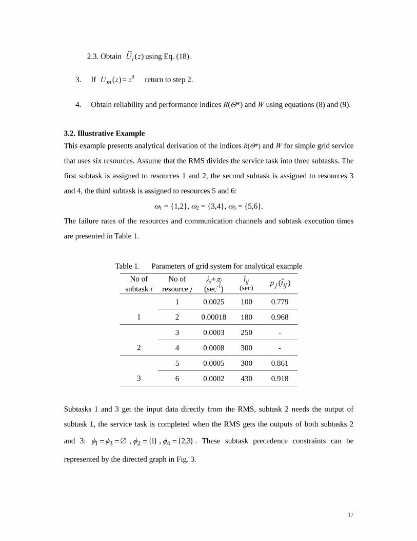
3.2. Illustrative Example This example presents analytical derivation of the indices R(Θ*) and W for simple grid service

that uses six resources. Assume that the RMS divides the service task into three subtasks. The

first subtask is assigned to resources 1 and 2, the second subtask is assigned to resources 3

and 4, the third subtask is assigned to resources 5 and 6:

ω1 = {1,2}, ω2 = {3,4}, ω3 = {5,6}.

The failure rates of the resources and communication channels and subtask execution times

are presented in Table 1.

Table 1. Parameters of grid system for analytical example

No of subtask i

No of resource j

λj+πj (sec-1) (sec)

ijt )ˆ( ijj tp

1

1 0.0025 100 0.779

2 0.00018 180 0.968

2

3 0.0003 250 -

4 0.0008 300 -

3

5 0.0005 300 0.861

6 0.0002 430 0.918

Subtasks 1 and 3 get the input data directly from the RMS, subtask 2 needs the output of

subtask 1, the service task is completed when the RMS gets the outputs of both subtasks 2

and 3: ∅== 31 φφ , }1{2 =φ , }3,2{4 =φ . These subtask precedence constraints can be

represented by the directed graph in Fig. 3.

18

1

3

2

4

Fig. 3. Subtask execution precedence constraints for analytical example

Since ∅== 31 φφ , the only realization of start times T1 and T3 is 0 and therefore,

U1(z)=U2(z)=z0 . According to step 2 of the algorithm we can obtain the u-functions

representing pmf of completion times 11~t , 12

~t , 35~t and 36

~t . In order to determine the

subtask execution time distributions for the individual resources, define the u-functions uij(z)

according to Table 1 and Eq. (9):

=×−−+×−= ∞zzzu )]1000025.0exp(1[)1000025.0exp()0,(~ 10011 0.779z100 + 0.221z∞.

In the similar way we obtain

)0,(~12 zu = 0.968z180 + 0.032z∞;

)0,(~35 zu = 0.861z300 + 0.139z∞; )0,(~

36 zu = 0.918z430 + 0.082z∞.

The u-function representing the pmf of the completion time for subtask 1 executed by both

resources 1 and 2 is

=)(~1 zU )0,(~

1 zu = )0,(~11 zu

min⊗ )0,(~

12 zu = (0.779z100 + 0.221z∞)min⊗ (0.968z180 + 0.032z∞)

=0.779z100 +0.214z180 + 0.007z∞.

The u-function representing the pmf of the completion time for subtask 3 executed by both

resources 5 and 6 is

=)(~3 zU )0,(~

3 zu = )(~35 zu

min⊗ )(~

36 zu = (0.861z300 + 0.139z∞)min⊗ (0.918z430 + 0.082z∞)

=0.861z300 +0.128z430 + 0.011z∞.

Execution of subtask 2 begins immediately after completion of subtask 1. Therefore,

U2(z) = )(~1 zU =0.779z100 +0.214z180 + 0.007z∞

19

(T2 has three realizations 100, 180 and ∞).

The u-functions representing the conditional pmf of the completion times for the subtask 2

executed by individual resources are obtained as follows.

∞+×−++×− −+= zezezu ]1[)100,(~ )250100(0003.0250100)250100(0003.023 =0.9z350+0.1z∞;

∞+×−++×− −+= zezezu ]1[)180,(~ )250180(0003.0250180)250180(0003.023 =0.879z430+0.121z∞;

∞=∞ zzu ),(~23 ;

∞+×−++×− −+= zezezu ]1[)100,(~ )300100(0008.0300100)300100(0008.024 =0.726z400+0.274z∞;

∞+×−++×− −+= zezezu ]1[)180,(~ )300180(0008.0300180)300180(0008.024 =0.681z480+0.319z∞;

∞=∞ zzu ),(~24 .

The u-functions representing the conditional pmf of subtask 2 completion time are:

=⊗= )100,(~)100,(~)100,(~24232 min

zuzuzu (0.9z350+0.1z∞)min⊗ (0.726z400+0.274z∞)

=0.9z350+0.073z400+0.027z∞;

=⊗= )180,(~)180,(~)180,(~24232 min

zuzuzu (0.879z430+0.121z∞)min⊗ (0.681z480+0.319z∞)

=0.879z430+0.082z480+0.039z∞;

.),(~),(~),(~24232 min

∞=∞⊗∞=∞ zzuzuzu

According to Eq. (18) the unconditional pmf of subtask 2 completion time is represented by

the following u-function

∞++= zzuzuzU 007.0)180,(~214.0)100,(~779.0)(~222

=0.779(0.9z350+0.073z400+0.027z∞)+0.214(0.879z430+0.082z480+0.039z∞)+0.007z∞

=0.701z350+0.056z400+0.188z430+0.018z480+0.037z∞

The service task is completed when subtasks 2 and 3 return their outputs to the RMS (which

corresponds to the beginning of subtask 4). Therefore, the u-function representing the pmf of

the entire service time is obtained as

)(~)(~)( 3max24 zUzUzU ⊗=

=(0.701z350+0.056z400+0.188z430+0.018z480+0.037z∞)max⊗ (0.861z300 +0.128z430 +

0.011z∞)=0.603z350 +0.049z400 +0.283z430 +0.017z480 +0.048z∞.

20

The pmf of the service time is:

Pr(T4 = 350) = 0.603; Pr(T4 = 400) = 0.049;

Pr(T4 = 430) = 0.283; Pr(T4 = 480) = 0.017; Pr(T4 = ∞) = 0.048.

From the obtained pmf we can calculate the service reliability using Eq. (8):

=*)(ΘR 0.603 for 350< *Θ ≤400; =*)(ΘR 0.652 for 400< *Θ ≤430;

=*)(ΘR 0.935 for 430< *Θ ≤480; =∞)(R 0.952

and the conditional expected service time according to Eq. (9):

W = (0.603×350 + 0.049×400 + 0.283×430 + 0.017×480) / 0.952 = 378.69 sec. 4. Tree Topology Grid Architecture In the star grid, the RMS is connected with each resource by one direct communication

channel (link). However, such approximation is not accurate enough even though it simplifies

the analysis and computation. For example, several resources located in a same local area

network (LAN) can use the same gateway to communicate outside the network. Therefore, all

these resources are not connected with the RMS through independent links. The resources are

connected to the gateway, which communicates with the RMS through one common

communication channel. Another example is a server that contains several resources (has

several processors that can run different applications simultaneously, or contains different

databases). Such a server communicates with the RMS through the same links. These

situations cannot be modeled using only the star topology grid architecture.

In this section, we present a more reasonable virtual structure which has a tree topology.

The root of the tree virtual structure is the RMS, and the leaves are resources, while the

branches of the tree represent the communication channels linking the leaves and the root.

Some channels are commonly used by multiple resources. An example of the tree topology is

given in Fig. 3 in which four resources (R1, R2, R3, R4) are available for a service.

The tree structure models the common cause failures in shared communication channels.

For example, in Fig. 3, the failure in channel L6 makes resources R1, R2, and R3 unavailable.

This type of common cause failure was ignored by the conventional parallel computing

models, and the above star-topology models. For small-area communication, such as a LAN

21

or a cluster, such assumption that ignores the common cause failures on communications is

acceptable because the communication time is negligible compared to the processing time.

However, for wide-area communication, such as the grid system, it is more likely to have

failure on communication channels. Therefore, the communication time cannot be neglected.

In many cases, the communication time may dominate the processing time due to the large

amount of data transmitted. Therefore, the virtual tree structure is an adequate model

representing the functioning of grid services.

L1

L2

L3L4

L5L6

J1, 48s

J1, 38s

J2, 35.5s

5Kbps0.005s-1

6Kbps

15Kbps 4Kbps

20Kbps

10Kbps0.003s-1

0.004s-1

0.002s-1

0.004s-1

0.008s-1

0.003s-1

0.004s-1

0.001s-1

RMS

R2

R3R4

R1

0.007s-1

J2, 25s

Fig. 3: A virtual tree structure of a grid service.

4.1. Algorithms for determining the pmf of the task execution time

With the tree-structure, the simple u-function technique is not applicable because it does not

consider the failure correlations. Thus, new algorithms are required. This section presents a

novel algorithm to evaluate the performance and reliability for the tree-structured grid service

based on the graph theory and the Bayesian approach.

4.1.1. Minimal Task Spanning Tree (MTST)

The set of all nodes and links involved in performing a given task form a task spanning tree.

This task spanning tree can be considered to be a combination of minimal task spanning trees

(MTST), where each MTST represents a minimal possible combination of available elements

22

(resources and links) that guarantees the successful completion of the entire task. The failure

of any element in a MTST leads to the entire task failure.

For solving the graph traversal problem, several classical algorithms have been suggested,

such as Depth-First search, Breadth-First search, etc. These algorithms can find all MTST

in an arbitrary graph (Dai et al., 2002). However, MTST in graphs with a tree topology can

be found in a much simpler way because each resource has a single path to the RMS, and the

tree structure is acyclic.

After the subtasks have been assigned to corresponding resources, it is easy to find all

combinations of resources such that each combination contains exactly m resources executing

m different subtasks that compose the entire task. Each combination determines exactly one

MTST consisting of links that belong to paths from the m resources to the RMS. The total

number of MTST is equal to the total number of such combinations N, where

∏=

=m

jjN

1||ω (22)

(see Example 4.2.1).

Along with the procedures of searching all the MTST, one has to determine the

corresponding running time and communication time for all the resources and links.

For any subtask j, and any resource k assigned to execute this subtask, one has the amount

of input and output data, the bandwidths of links, belonging to the corresponding paths γk,

and the resource processing time. With these data, one can obtain the time of subtask

completion (see Example 4.2.2).

Some elements of the same MTST can belong to several paths if they are involved in data

transmission to several resources. To track the element involvement in performing different

subtasks and to record the corresponding times in which the element failure causes the failure

of a subtask, we create the lists of two-field records for each subtask in each MTST. For any

MTST Si (1≤i≤N), and any subtask j (1≤j≤m), this list contains the names of the elements

involved in performing the subtask j, and the corresponding time of subtask completion yij

(see Example 4.2.3). Note that yij is the conditional time of subtask j completion given only

MTST i is available.

23

Note that a MTST completes the entire task if all of its elements do not fail by the

maximal time needed to complete subtasks in performing which they are involved. Therefore,

when calculating the element reliability in a given MTST, one has to use the corresponding

record with maximal time.

4.1.2. pmf of the task execution time

Having the MTST, and the times of their elements involvement in performing different

subtasks, one can determine the pmf of the entire service time.

First, we can obtain the conditional time of the entire task completion given only MTST

Si is available as

)(max1

}{ ijmj

i yY≤≤

= for any 1≤i≤N: (23)

For a set ψ of available MTST, the task completion time is equal to the minimal task

completion times among the MTST.

⎥⎦

⎤⎢⎣

⎡==

≤≤∈∈)(maxmin)(min

1}{ ij

mjii

iyYY

ψψψ . (24)

Now, we can sort the MTST in an increasing order of their conditional task completion

times }{iY , and divide them into different groups containing MTST with identical conditional

completion time. Suppose there are K such groups denoted by KGGG ,...,, 21 where

NK ≤≤1 , and any group iG contains MTST with identical conditional task completion

times iΘ ( ).0 21 KΘ...ΘΘ <<<≤ Then, it can be seen that the probability

)(Pr ii ΘΘQ == can be obtained as

)(Pr 121 E,...,E,E,EQ iiii −−= (25)

where iE is the event when at least one of MTST from the group iG is available, and iE

is the event when none of MTST from the group iG is available.

Suppose the MTST in a group iG are arbitrarily ordered, and ijF (j=1,2,…, iN )

represents an event when the j-th MTST in the group is available. Then, the event iE can be

24

expressed by

∪iN

jiji FE

1=

= , (26)

and (25) takes the form

),...,,,Pr( 121 EEEE iii −− = ),...,,,Pr( 1211

EEEF ii

N

jij

i

−−=∪ . (27)

Using the Bayesian theorem on conditional probability, we obtain from (27) that

Qi = ( ) ( )∑=

−−−⋅iN

jijiijijiij FEEEFFFF

11211)2()1( ,,,,,...,,PrPr . (28)

The probability ( )ijFPr can be calculated as a product of the reliabilities of all the

elements belonging to the j-th MTST from group Gi.

The probability ( )ijiijiji FEEEFFF 1211)2()1( ,,,,,...,,Pr −−− can be computed by the

following two-step algorithm (see Example 4.2.4).

Step 1: Identify failures of all the critical elements’ in a period of time (defined by the

start and end time), during which they lead to the failures of any MTST from groups Gm for

m=1,2,…i-1 (events mE ), and any MTST Sk from group Gi for k=1,2,…, 1−j (events ikF ),

but do not affect the MTST Sj from group Gi.

Step 2: Ggenerate all the possible combinations of the identified critical elements that

lead to the event ijiijiji FEEEFFF 1211)2()1( ,,,,,...,, −−− using a binary search, and compute the

probabilities of those combinations. The sum of the probabilities obtained is equal to

( )ijiijiji FEEEFFF 1211)2()1( ,,,,,...,,Pr −−− . When calculating the failure probabilities of

MTSTs' elements, the maximal time from the corresponding records in a list for the given

MTST should be used. The algorithm for obtaining the probabilities },,Pr{ 1

___

2

___

1 ii EEEE −

can be found in Dai et al. (2002).

Having the conditional task completion times }{iY for different MTST, and the

corresponding probabilities Qi, one obtains the task completion time distribution ( ii QΘ , ),

1≤i≤K, and can easily calculate the indices (8) & (9) (see Example 4.2.5).

25

4.2. Illustrative Example

Consider the virtual grid presented in Fig. 3, and assume that the service task is divided into

two subtasks J1 assigned to resources R1 & R4, and J2 assigned to resources R2 & R3. J1,

and J2 require 50Kbits, and 30Kbits of input data, respectively, to be sent from the RMS to

the corresponding resource; and 100Kbits, and 60Kbits of output data respectively to be sent

from the resource back to the RMS.

The subtask processing times for resources, bandwidth of links, and failure rates are

presented in Fig. 3 next to the corresponding elements.

4.2.1. The service MTST

The entire graph constitutes the task spanning tree. There exist four possible

combinations of two resources executing both subtasks: {R1, R2}, {R1, R3}, {R4, R2}, {R4,

R3}. The four MTST corresponding to these combinations are: S1: {R1, R2, L1, L2, L5, L6};

S2: {R1, R3, L1, L3, L5, L6}; S3: {R2, R4, L2, L5, L4, L6}; S4: {R3, R4, L3, L4, L6}.

4.2.2.. Parameters of MTSTs' paths

Having the MTST, one can obtain the data transmission speed for each path between the

resource, and the RMS (as minimal bandwidth of links belonging to the path); and calculate

the data transmission times, and the times of subtasks' completion. These parameters are

presented in Table 2. For example, resource R1 (belonging to two MTST S1 & S2) processes

subtask J1 in 48 seconds. To complete the subtask, it should receive 50Kbits, and return to the

RMS 100Kbits of data. The speed of data transmission between the RMS and R1 is limited

by the bandwidth of link L1, and is equal to 5 Kbps. Therefore, the data transmission time is

150/5=30 seconds, and the total time of task completion by R1 is 30+48=78 seconds.

Table 2: Parameters of the MTSTs' paths

Elements, subtasks R1, J1 R2, J2 R3, J2 R4, J1 Data transmission speed (Kbps) 5 6 4 10

Data transmission time (s) 30 15 22.5 15 Processing time (s) 48 25 35.5 38

Time to subtask completion (s) 78 40 58 53

4.2.3.. List of MTST elements

26

Now one can obtain the lists of two-field records for components of the MTST.

S1: path for J1:(R1,78); (L1,78); (L5,78); (L6,78); path for J2: (R2,40); (L2,40); (L5,40);

(L6,40).

S2: path for J1: (R1,78), (L1,78), (L5,78), (L6,78); path for J2: (R3,58), (L3,58), (L6,58).

S3: path for J1: (R4,53), (L4,53); path for J2: (R2,40), (L2,40), (L5,40), (L6,40).

S4: path for J1: (R4,53), (L4,53); path for J2: (R3,58), (L3,58), (L6,58).

4.2.4. pmf of task completion time

The conditional times of the entire task completion by different MTST are

Y1=78; Y2=78; Y3=53; Y4=58.

Therefore, the MTST compose three groups:

G1 = {S3} with Θ1 = 53; G2 = {S4} with Θ2= 58; and G3 = {S1, S2} with Θ3 = 78.

According to (25), we have for group G1: Q1=Pr(E1)=Pr(S3). The probability that the

MTST S3 completes the entire task is equal to the product of the probabilities that R4, and L4

do not fail by 53 seconds; and R2, L2, L5, and L6 do not fail by 40 seconds.

Pr(Θ=53)=Q1=exp(−0.004×53)exp(−0.004×53)exp(−0.008×40)

×exp(−0.003×40)exp(−0.001×40)exp(−0.002×40) = 0.3738.

Now we can calculate Q2 as

Q2 = ),Pr( 12 EE = ( ) ( )21121 PrPr FEF = ( ) ( )211121 PrPr FFF = ( ) ( )434 PrPr SSS

because G2, and G1 have only one MTST each. The probability that the MTST S4 completes

the entire task ( )4Pr S is equal to the product of probabilities that R3, L3, and L6 do not fail

by 58 seconds; and R4, and L4 do not fail by 53 seconds.

( )4Pr S = )58002.0exp()58004.0exp()53004.0exp()58003.0exp()53004.0exp( ×−×−×−×−×−

= 0.3883

To obtain ( )43Pr SS , one first should identify the critical elements according to the algorithm

presented in the Dai et al. (2002). These elements are R2, L2, and L5. Any failure occurring

in one of these elements by 40 seconds causes failure of S3, but does not affect S4. The

probability that at least one failure occurs in the set of critical elements is

27

( )43Pr SS = )40001.0exp()40003.0exp()40008.0exp(1 ×−×−×−− = 0.3812.

Then,

Pr(Θ =58) = ),Pr( 12 EE = ( )4Pr S ( )43Pr SS = 3812.03883.0 × =0.1480.

Now one can calculate Q3 for the last group G3 = {S1, S2} corresponding to Θ3 = 78 as

Q3 = ),,Pr( 123 EEE = ( ) ( ) ( ) ( )32213132312131 ,,PrPr,PrPr FEEFFFEEF +

= ( ) ( ) ( ) ( )243121431 ,,PrPr,PrPr SSSSSSSSS +

The probability that the MTST S1 completes the entire task is equal to the product of the

probabilities that R1, L1, L5, and L6 do not fail by 78 seconds; and R2, and L2 do not fail by

40 seconds.

( ).1999.0)78002.0exp()78001.0exp(

)40003.0exp()78005.0exp()40008.0exp()78007.0exp(Pr 1=×−×−×

×−×−×−×−=S

The probability that the MTST S2 completes the entire task is equal to the product of the

probabilities that R1, L1, L5, and L6 do not fail by 78 seconds; and R3, and L3 do not fail by

58 seconds.

( ).2068.0)78002.0exp()78001.0exp(

)58004.0exp()78005.0exp()58003.0exp()78007.0exp(Pr 2=×−×−×

×−×−×−×−=S

To obtain ( )143,Pr SSS , one first should identify the critical elements. Any failure of

either R4 or L4 in the time interval from 0 to 53 seconds causes failures of both S3, and S4;

but does not affect S1. Therefore,

( )143 ,Pr SSS = )53004.0exp()53004.0exp(1 ×−×−− =0.3456.

The critical elements for calculating ( )2431 ,,Pr SSSS are R2, and L2 in the interval from 0 to

40 seconds; and R4, and L4 in the interval from 0 to 53 seconds. The failure of both elements

in any one of the following four combinations causes failures of S3, S4, and S1, but does not

affect S2:

1. R2 during the first 40 seconds, and R4 during the first 53 seconds;

2. R2 during the first 40 seconds, and L4 during the first 53 seconds;

3. L2 during the first 40 seconds, and R4 during the first 53 seconds; and

28

4. L2 during the first 40 seconds, and L4 during the first 53 seconds.

Therefore,

( )2431 ,,Pr SSSS = ∏ ∏= =

⎥⎦

⎤⎢⎣

⎡⋅−−−

4

1

2

1

)](exp1[11i

ijijj

tλ =0.1230,

where ijλ is the failure rate of the j-th critical element in the i-th combination (j=1,2),

(i=1,2,3,4); and ijt is the duration of the time interval for the corresponding critical element.

Having the values of ( ) ( ) ( )14321 ,Pr,Pr,Pr SSSSS , and ( )2431 ,,Pr SSSS , one can calculate

Pr(Θ =78)= Q3 =0.1999×0.3456+0.2068×0.1230=0.0945.

After obtaining Q1, Q2, and Q3, one can evaluate the total task failure probability as

Pr(Θ =∞)=1-Q1-Q2-Q3=1-0.3738-0.1480-0.0945=0.3837,

and obtain the pmf of service time presented in Table 3.

Table 3: pmf of service time.

iΘ iQ Θi iQ

53 0.3738 19.8114 58 0.1480 8.584 78 0.0945 7.371 ∞ 0.3837 ∞

4.2.5. Calculating the reliability indices.

From Table 3, weone obtains the probability that the service does not fail as

6164.0)( 321 =++=∞ QQQR ,

the probability that the service time is not greater than a pre-specified value of θ*=60 seconds

as

5218.01480.03738.0*)(1*)(3

1=+=<⋅= ∑

=θθ i

ii ΘQR ,

and the expected service execution time given that the system does not fail as

025.586164.0/7664.35)(/3

1==∞= ∑

=RQΘW i

ii seconds.

29

4.3. Parameterization and Monitoring

In order to obtain the reliability and performance indices of the grid service one has to know

such model parameters as the failure rates of the virtual links and the virtual nodes, and

bandwidth of the links. It is easy to estimate those parameters by implementing the

monitoring technology.

A monitoring system (called Alertmon Network Monitor,

http://www.abilene.iu.edu/noc.html) is being applied in the IP-grid (Indiana Purdue Grid)

project (www.ip-grid.org), to detect the component failures, to record service behavior, to

monitor the network traffics and to control the system configurations.

With this monitoring system, one can easily obtain the parameters required by the grid

service reliability model by adding the following functions in the monitoring system:

1) Monitoring the failures of the components (virtual links and nodes) in the grid service,

and recording the total execution time of those components. The failure rates of the

components can be simply estimated by the number of failures over the total

execution time.

2) Monitoring the real time network traffic of the involved channels (virtual links) in

order to obtain the bandwidth of the links.

To realize the above monitoring functions, network sensors are required. We presented a type

of sensors attaching to the components, acting as neurons attaching to the skins. It means the

components themselves or adjacent components play the roles of sensors at the same time

when they are working. Only a little computational resource in the components is used for

accumulating failures/time and for dividing operations, and only a little memory is required

for saving the data (accumulated number of failures, accumulated time and current

bandwidth). The virtual nodes that have memory and computational function can play the

sensing role themselves; if some links have no CPU or memory then the adjacent processors

or routers can perform this data collecting operations. Using such self-sensing technique

avoids overloading of the monitoring center even in the grid system containing numerous

components. Again, it does not affects the service performance considerably since only small

part of computation and storage resources is used for the monitoring. In addition, such

self-sensing technique can also be applied in monitoring other measures.

30

When evaluating the grid service reliability, the RMS automatically loads the required

parameters from corresponding sensors and calculates the service reliability and performance

according to the approaches presented in the previous sections. This strategy can also be used

for implementing the Autonomic Computing concept.

5. Conclusions Grid computing is a newly developed technology for complex systems with large-scale

resource sharing, wide-area communication, and multi-institutional collaboration. Although

the developmental tools and techniques for the grid have been widely studied, grid reliability

analysis and modeling are not easy because of their complexity of combining various failures.

This chapter introduced the grid computing technology and analyzed the grid service

reliability and performance under the context of performability. The chapter then presented

models for star-topology grid with data dependence and tree-structure grid with failure

correlation. Evaluation tools and algorithms were presented based on the universal generating

function, graph theory, and Bayesian approach. Numerical examples are presented to

illustrate the grid modeling and reliability/performance evaluation procedures and

approaches.

Future research can extend the models for grid computing to other large-scale distributed

computing systems. After analyzing the details and specificity of corresponding systems, the

approaches and models can be adapted to real conditions. The models are also applicable to

wireless network that is more failure prone.

Hierarchical models can also be analyzed in which output of lower level models can be

considered as the input of the higher level models. Each level can make use of the proposed

models and evaluation tools. References: Abramson, D., Buyya, R., Giddy, J. (2002), A computational economy for grid computing

and its implementation in the Nimrod-G resource broker, Future Generation Computer Systems, vol. 18, no. 8, pp. 1061-1074.

Berman, F., Wolski, R., Casanova, H., Cirne, W., Dail, H., Faerman, M., Figueira, S., Hayes, J., Obertelli, G., Schopf, J., Shao, G., Smallen, S., Spring, N., Su, A., Zagorodnov, D., (2003), Adaptive computing on the Grid using AppLeS, IEEE Transactions on Parallel

31

and Distributed Systems, vol.14, no.14, pp.369 – 382.

Cao, J., Jarvis, S.A., Saini, S., Kerbyson, D.J., Nudd, G.R. (2002), ARMS: An agent-based resource management system for grid computing, Scientific Programming, vol. 10, no. 2, pp. 135-148.

Chen D. J., Huang T. H., (1992), Reliability analysis of distributed systems based on a fast reliability algorithm, IEEE Transactions on Parallel and Distributed Systems, vol. 3 , no. 2 , pp. 139 – 154.

Chen, D.J., Chen, R.S., Huang, T.H. (1997), A heuristic approach to generating file spanning trees for reliability analysis of distributed computing systems, Computers and Mathematics with Application, vol. 34, pp. 115-131.

Dai, Y.S., Levitin, G. (2006), Reliability and performance of tree-structured grid services, IEEE Transactions on Reliability, vol. 55, no. 2, pp. 337-349, 2006.

Dai, Y.S., Xie, M., Poh, K.L. (2005), Markov renewal models for correlated software failures of multiple types, IEEE Transactions on Reliability, vol. 54, no. 1, pp. 100-106.

Dai, Y.S., Xie, M. and Poh, K.L. (2006), Availability modelling and cost optimization for the grid resource management system, IEEE Transactions on Systems, Man, and Cybernetics, Part A, In Press. (Accepted)

Dai, Y.S., Pan, Y., Zou, X.K. (2006), A hierarchical modelling and analysis for grid service reliability, IEEE Transactions on Computers, Conditionally Accepted.

Dai, Y.S., Xie, M. and Poh, K.L. (2002), Reliability Analysis of Grid Computing Systems, IEEE Pacific Rim International Symposium on Dependable Computing (PRDC2002), IEEE Computer Press, pp. 97-104.

Dai, Y.S., Xie, M., Poh, K.L., Liu, G.Q. (2003), A study of service reliability and availability for distributed systems, Reliability Engineering and System Safety, vol. 79, no. 1, pp. 103-112.

Dai, Y.S., Xie, M., Poh, K.L., Ng, S.H. (2004), A model for correlated failures in N-version programming, IIE Transactions, vol. 36, no. 12, pp. 1183-1192.

Das, S.K., Harvey, D.J., Biswas, R., (2001), Parallel processing of adaptive meshes with load balancing, IEEE Transactions on Parallel and Distributed Systems, vol. 12, no. 12, pp.1269 – 1280.

Ding, Q., Chen, G.L., Gu, J. (2002), A unified resource mapping strategy in computational grid environments, Journal of Software, vol. 13, no. 7, pp. 1303-1308.

Foster, I., Kesselman, C. (2003), The Grid 2: Blueprint for a New Computing Infrastructure, Morgan-Kaufmann.

Foster, I., Kesselman, C. and Tuecke, S. (2001), The anatomy of the grid: Enabling scalable virtual organizations, International Journal of High Performance Computing Applications, vol. 15, pp. 200-222.

Foster, I., Kesselman, C., Nick, J.M., Tuecke, S. (2002), Grid services for distributed system

32

integration, Computer, vol. 35, no. 6, pp. 37-46. Grassi, V., Donatiello L., Iazeolla G., (1988) Performability evaluation of multicomponent

fault tolerant systems, IEEE Transactions on Reliability, vol. 37, no. 2, pp. 216-222.

Krauter, K., Buyya, R., Maheswaran, M. (2002), A taxonomy and survey of grid resource management systems for distributed computing, Software - Practice and Experience, vol. 32, no. 2, pp. 135-164.

Kumar, A. (2000) An efficient SuperGrid protocol for high availability and load balancing, IEEE Transactions on Computers, vol. 49, no. 10, pp. 1126-1133.

Kumar, V.K.P., Hariri, S., Raghavendra, C.S. (1986), Distributed program reliability analysis, IEEE Transactions on Software Engineering, vol. SE-12, pp. 42-50.

Levitin, G., Dai, Y.S., Ben-Haim, H. (2006), Reliability and performance of star topology grid service with precedence constraints on subtask execution, IEEE Transactions on Reliability, 55(3), pp. 507-515.

Levitin, G., Dai, Y.S., Xie, M., Poh, K.L (2003), Optimizing survivability of multi-state systems with multi-level protection by multi-processor genetic algorithm, Reliability Engineering & System Safety, vol. 82, pp. 93-104.

Lin, M.S., Chang, M.S., Chen, D.J., Ku, K.L. (2001), The distributed program reliability analysis on ring-type topologies, Computers and Operations Research, vol. 28, pp. 625-635.

Liu, G.Q., Xie, M., Dai, Y.S., Poh, K.L. (2004), On program and file assignment for distributed systems, Computer Systems Science and Engineering, vol. 19, no. 1, pp. 39-48.

Livny, M., Raman, R. (1998), High-throughput resource management, In The Grid: Blueprint for a New Computing Infrastructure, San Francisco, CA: Morgan-Kaufmann, pp. 311-338.

Meyer, J. (1980), On evaluating the performability of degradable computing systems, IEEE Transactions on Computers, vol. 29, pp. 720-731.

Nabrzyski, J., Schopf, J.M., Weglarz, J. (2003), Grid Resource Management, Kluwer Publishing.

Pham, H. (2000), Software Reliability, Singapore: Springer-Verlag. Tai, A., Meyer J., Avizienis A. (1993), Performability enhancement of fault-tolerant

software, IEEE Transactions on Reliability, vol. 42, no. 2, pp. 227-237.

Xie, M. (1991), Software Reliability Modeling, World Scientific Publishing Company.

Xie, M., Dai, Y.S., Poh, K.L. (2004), Computing Systems Reliability: Models and Analysis, Kluwer Academic Publishers: New York, NY, U.S.A.

Yang, B. and Xie, M. (2000), A study of operational and testing reliability in software reliability analysis, Reliability Engineering & System Safety, vol. 70, pp. 323-329.