Reliability analysisOSKAR LARSSON

Reliability as a concept

General definition

The ability to meet specific requirements under a specified period

Mathematical definition in structural reliability

The probability that a system does not reach a defined limit state under a given reference period.

2

Background

• During the second world war it became evident that the reliability of complex technical installations was a problem

• As an example the modern warships at the time were only operational for attack/defence in about 60 % of the time

• Similar effects were observed on the reliability of e.g. the V1l V2 rocket systems -the first of many launches were unsuccessful

• These events were the real initiators of the reliability theory for technical components and systems

3

Background

• lnitially the reliability theory was developed for systems with a large number of {semi-} identical components subject to the same exposure conditions

– electrical systems {bulbs, switches, .. }

• and later on to– nuclear power installations {valves, pipes, pumps, .. }– chemical plants (pipes, pressure vessels, valves,

pumps, .. }– manufacturing plants (pumps, compressors,

conveyers, .. }4

Background

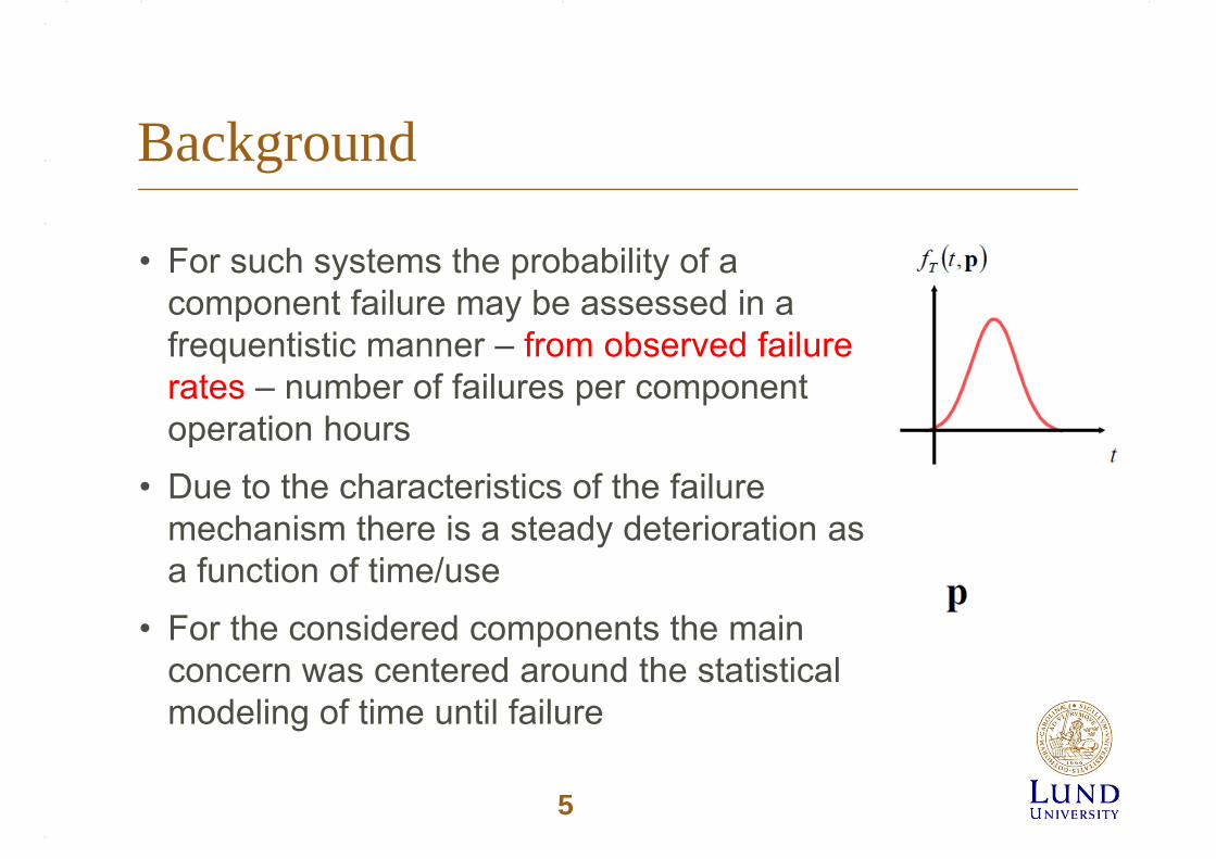
• For such systems the probability of a component failure may be assessed in a frequentistic manner – from observed failure rates – number of failures per component operation hours

• Due to the characteristics of the failure mechanism there is a steady deterioration as a function of time/use

• For the considered components the main concern was centered around the statistical modeling of time until failure

5

Background

• For technical systems such as structures and structural components the classical reliability analysis is of limited use because

– all structural components are unique– the failure mechanism tends to be related to extreme

load events exceeding the residual capacity of the component- not the direct effect of deterioration alone

• For such systems a different approach is thus required, namely

– an individual modeling of both the resistance as a function of time and the loading as a function of time

6

Connection to previous lectures

• Basic statistics:– Distributions, (mean, std. deviation, parameters)– Probability of failure– Standard normal distribution

• Introduction– Codes and standards, partial coefficients– Limit states– Modeling of uncertainties

7

Methods to measure reliability

• Level I methodUncertain parameters are modelled by one characteristicvalue, e.g. code based on partial coefficent method

• Level II methodUncertain parameters modelled by the mean values and the standard deviations and by the correlation coefficietnsbetween stochastic vairables. The stochastic variables areimplicitly assumed to be normally distributed. The reliabilityindex method is an example of a level II method

8

Methods to measure reliability

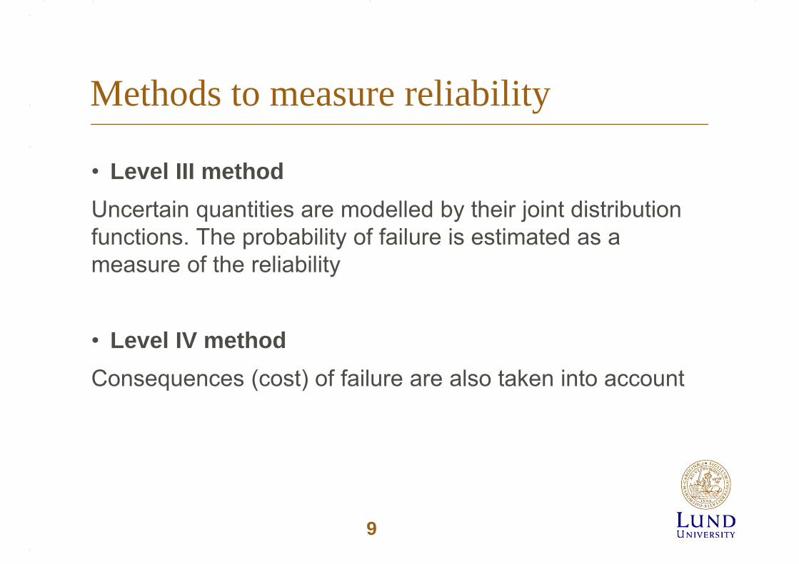
• Level III methodUncertain quantities are modelled by their joint distribution functions. The probability of failure is estimated as a measure of the reliability

• Level IV methodConsequences (cost) of failure are also taken into account

9

Deterministic reliability measures(Level I)

• Single safety factor

• Partial safety factors

10

Safety factor

• Safety factor is a traditional measure on reliability

Design condition: G+Q<R/s

where s is safety factor > 1

• G,Q and R are ”nominal” values not necessarily definedin statistical terms

• Differences in uncertainty between basic parameters arenot considered, e.g. G och Q.

11

Partial safety factor format

Index k denotes characteristic value

Characteristic values are defined in statistical terms

i denote partial safety factors reflecting different degree of uncertainty for basic parameters

dQkGkR

kd SQG

RR )(

12

Implicit and generic risk analysis behind modern structural codes

• Consequences and risk acceptance in the society are implicitly considered in modern structural codes

• The results are presented in terms of required levels of formal reliability in different situations

• This means that the decision problem when designing a structure is transformed to a verification that the probability of violation of the limit state is lower that a prescribed level.

• Modern structural codes are often called limit state design codes

13

Probabilistic reliability measures

14

Structural reliability

Reliability of structures cannot be assessed through failure rates because:

- Structures are unique in nature

- Structural failures normally take place due to extreme loads exceeding the residualstrength

Therefore in structural reliability, models are established for resistances R and loads S individually and the structural reliability is assessed through the probability of failure

15

Probability of failure, reliability

Probability of failure pf = P(R-S<0)

Reliability = 1- pf

Design of a new structure

Design the structure so that pf is less than target value

Verification of existing structure

Check if pf is less than target value

16

Main steps in reliability analysis

1. Select a target reliability level (safety or consequence class)

2. Identify significant failure modes (deflection, bending)3. Formulate limit state functions (g(E,R) = MEd – MRd = 0)4. Identify stochastic variables and deterministic

parameters. Specify distribution types and statistical parameters

5. Estimate reliability of each failure mode6. Change design if reliabiliy does not meat target reliabilty7. Evaluate reliability result by a sensitivity analysis

17

Structural Engineering Decision Problem:

Optimal Design:

01 F D DD

F F DE B I P C C CE BC

P C

Benefit of the Structure in Service

Expected Benefit of the Structure

Reliability Risk

Benefit

Risk

Cost

But what is a proper target reliability???

18

Theory of StructuralReliability

19

FailureIn general defined as: capacity < demand

resistance < load effect

e.g. a beam in bending:

4mG lf W r s

BUT - resistance and load effect are uncertain !!!First assume that r and s are Normal distributed random variables with known mean values and standard deviations.

20

Probability of failure

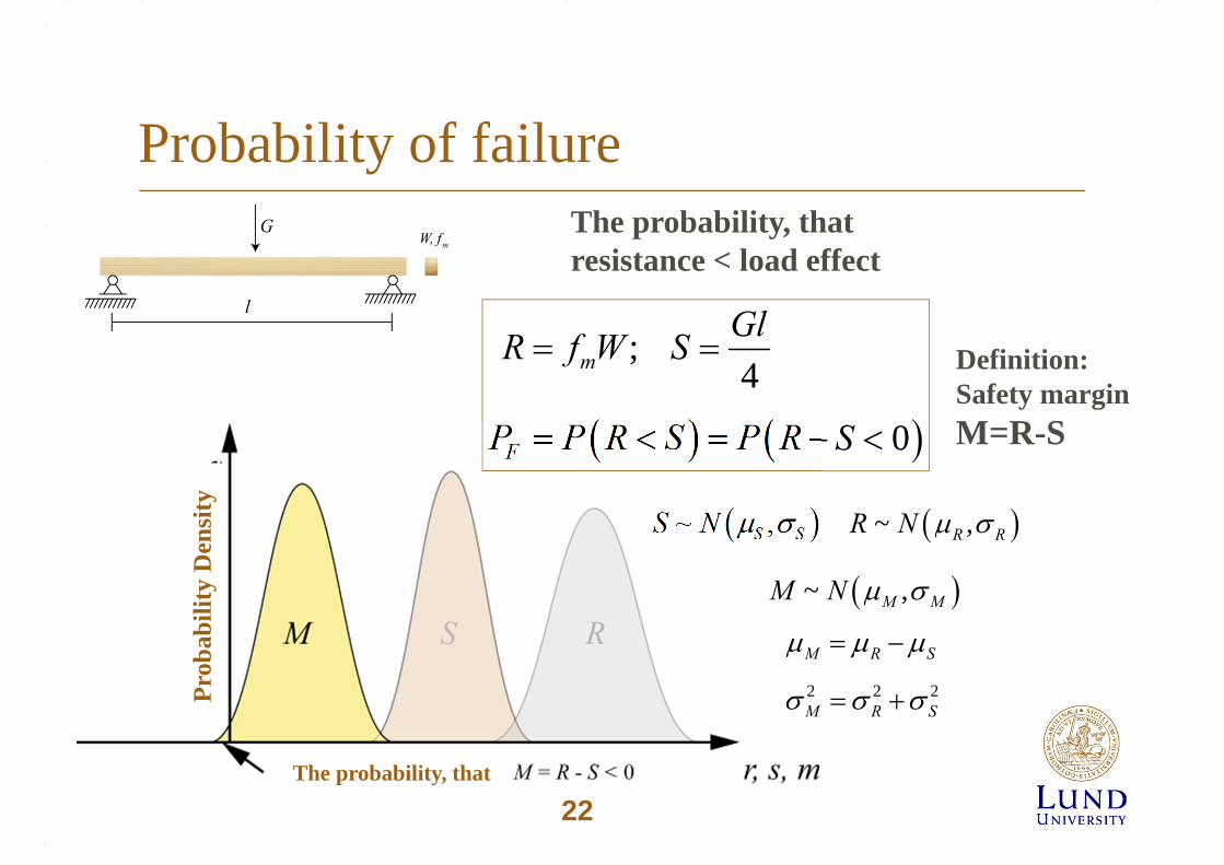
~ ,S SS N ~ ,R RR N

; 4

0

m

F

GlR f W S

P P R S P R S

The probability, that resistance < load effect

21

Probability of failure

~ ,S SS N ~ ,R RR N

; 4

0

m

F

GlR f W S

P P R S P R S

The probability, that resistance < load effect

Prob

abili

ty D

ensi

ty

~ ,M MM N

2 2 2

M R S

M R S

The probability, that

Definition:Safety margin M=R-S

22

Probability of failure

; 4

0 0

m

F

GlR f W S

P P R S P R S P M

0 0 M

F MM

P f m dm

The probability, that resistance < load effect

Prob

abili

ty D

ensi

ty

The probability, that23

0 0 M

F MM

P f m dm

Probability of failure

; 4

0 0

m

F

GlR f W S

P P R S P R S P M

The probability, that resistance < load effect

Prob

abili

ty D

ensi

ty

The probability, that

Mf m

Reliability Index

24

Reliability Index (Safety index)

Prob

abili

ty D

ensi

ty

MF

M

P

Geometrical interpretation:

25

Reliability IndexPr

obab

ility

Den

sity

M

FM

P

Geometrical interpretation:

0 0.51 0.1586552 0.022753 0.001354 3.17E‐055 2.87E‐076 9.87E‐107 1.28E‐128 6.22E‐16

FP

26

Safety class

• The reliability index (probability of failure) is governing the safety class used in the partial safety factor method

Safety class

Reliability index

Probability of failure

Part. Safety factor

1 Less serious

3,7 10-4 0,83

2 Serious 4,3 10-5 0,913 Very serious

4,7 10-6 1,0

27

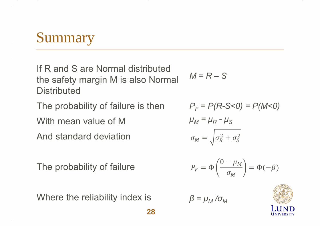
Summary

If R and S are Normal distributed the safety margin M is also Normal DistributedThe probability of failure is thenWith mean value of MAnd standard deviation

The probability of failure

Where the reliability index is

M = R – S

PF = P(R-S<0) = P(M<0)μM = μR - μS

β = μM /σM

Ф0

Ф

28

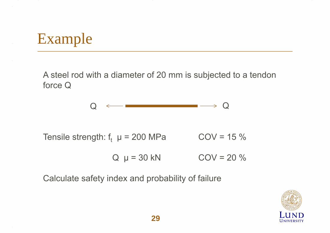
Example

A steel rod with a diameter of 20 mm is subjected to a tendon force Q

Tensile strength: ft μ = 200 MPa COV = 15 %

Q μ = 30 kN COV = 20 %

Calculate safety index and probability of failure

QQ

29

Reliability Analysis, the general case

Limit state function general case

In the general case the resistance and the load may be defined in terms of functions where X are basic random variables

R = f1(X), S = f2(X)

M= R-S = f1(X)-f2(X) = g(X)

The limit state function should be defined so that

M= g(X) > 0 corresponds to the safe state

M= g(X) < 0 corresponds to the failure state

30

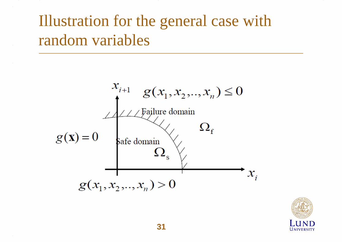
Illustration for the general case with random variables

31

Probability of failure Pf

Pf =P(M0) = P(g(X)0)

Introduce the joint probability density function fX(X)

Then

f

dXXfP Xf

)(

where f is the failure region defined by the limit state function

X = (x1,.....xn )

32

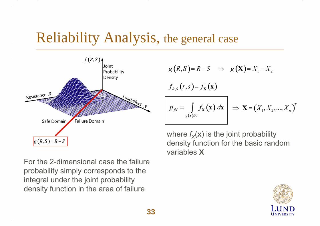
Reliability Analysis, the general case

where fX(x) is the joint probabilitydensity function for the basic random variables X

For the 2-dimensional case the failure probability simply corresponds to the integral under the joint probability density function in the area of failure

33

Analysis methods in reliability analysis

• Analytical methods (only in very special cases)

• First Order Reliability Methods (FORM)

• Second Order Reliability Methods (SORM)

• Simulation techniques

34

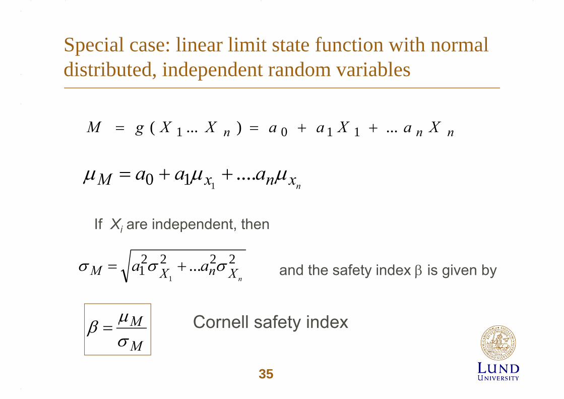
Special case: linear limit state function with normal distributed, independent random variables

nnn XaXaaXXgM ...)...( 1101

nxnxM aaa ....110

If Xi are independent, then

22221 ...

1 nXnXM aa and the safety index is given by

M

M Cornell safety index

35

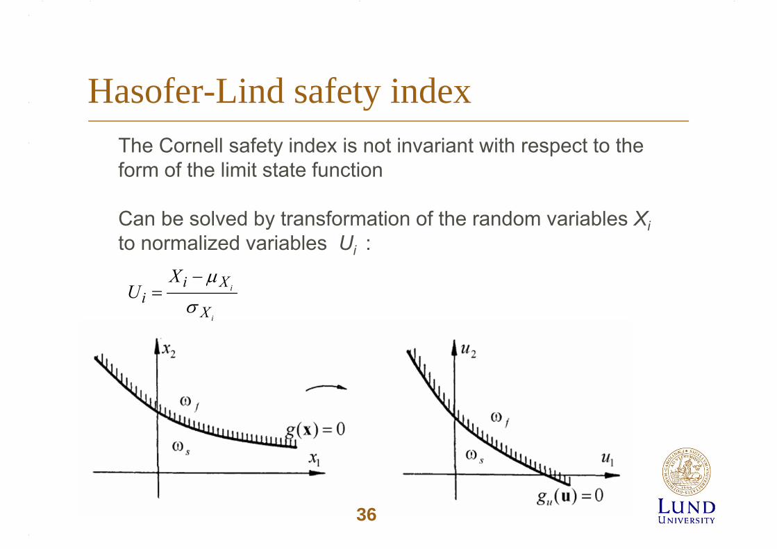
Hasofer-Lind safety indexThe Cornell safety index is not invariant with respect to the form of the limit state function

Can be solved by transformation of the random variables Xito normalized variables Ui :

i

i

X

Xii

XU

36

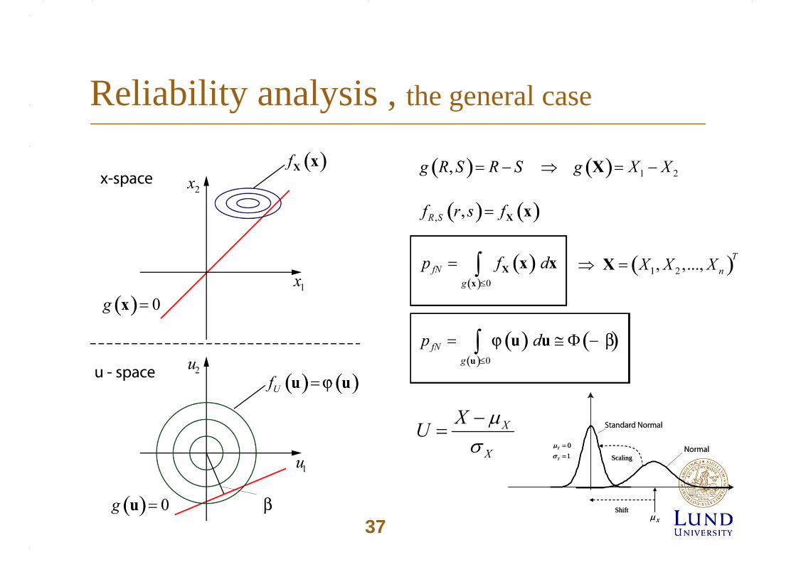
Reliability analysis , the general case

X

X

XU

Standard Normal

Normal

XShift

Scaling

01

Y

Y

Standard Normal

Normal

XShift

Scaling

01

Y

Y

37

Non-linear failure function

The failure function can be linearized by Taylor expansion:

)()( *

1

*

*

uUUgugM i

uu

n

i

where u* is the design point

This is the first order approximation (FORM)If one more term is included in the expansion we have a “second order” approximation (SORM)

Note that u* is not known at the outset, and has to be found by iteration

38

Geometrical interpretation

The safety index is the shortest distance from the failure surface to the origin in the normalised space U

The point u* on the failure surface is called the design point

The components of the unit vector of the normal to the failure surface in the point u* describes the relative importance (or sensitivities) of the random variables.

39

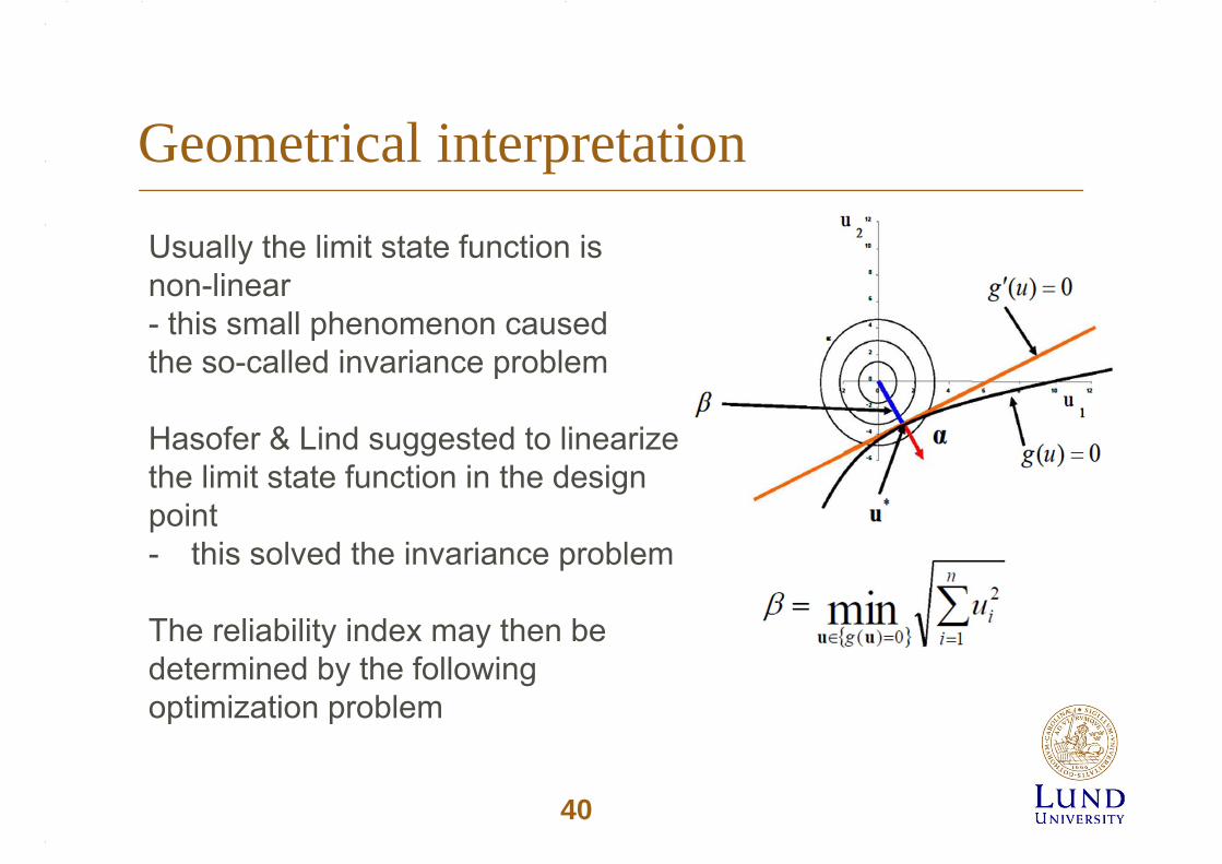
Geometrical interpretation

Usually the limit state function isnon-linear- this small phenomenon causedthe so-called invariance problem

Hasofer & Lind suggested to linearizethe limit state function in the designpoint- this solved the invariance problem

The reliability index may then bedetermined by the followingoptimization problem

40

Iteration processThe optimization problem can be formulatedas an iteration problem

1) the design point is determined as

2) the normal vector to the limit statefunction is determined as

3) the safety index is determined as

4) a new design point is determined as

5) the above steps are continued untilconvergence in is attained

u = β · α

41

Iteration process

• There are two alternative procedures for solving the iteration problem:

- The simultaneous equation procedure (shown in the next example)

- The matrix procedure

42

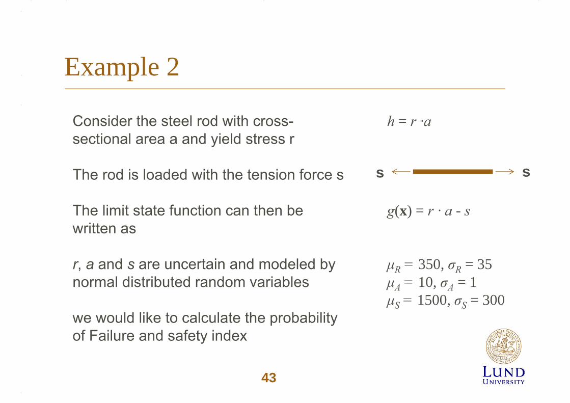
Example 2

Consider the steel rod with cross-sectional area a and yield stress r

The rod is loaded with the tension force s

The limit state function can then be written as

r, a and s are uncertain and modeled bynormal distributed random variables

we would like to calculate the probability of Failure and safety index

h = r ·a

g(x) = r · a - s

μR = 350, σR = 35 μA = 10, σA = 1 μS = 1500, σS = 300

ss

43

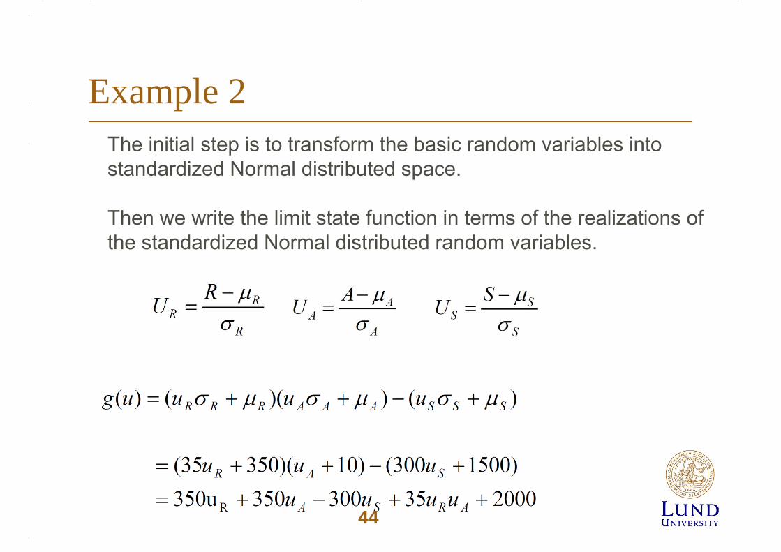
Example 2The initial step is to transform the basic random variables into standardized Normal distributed space.

Then we write the limit state function in terms of the realizations of the standardized Normal distributed random variables.

44

Example 2Choose an arbitrary first design point u = βα

Limit state function

g(u) = 350βαR + 350βαA - 300βαS + 35 βαR βαA + 2000

The safety index is determined by

g(u) = 0

This gives

2000350 350 300 35

45

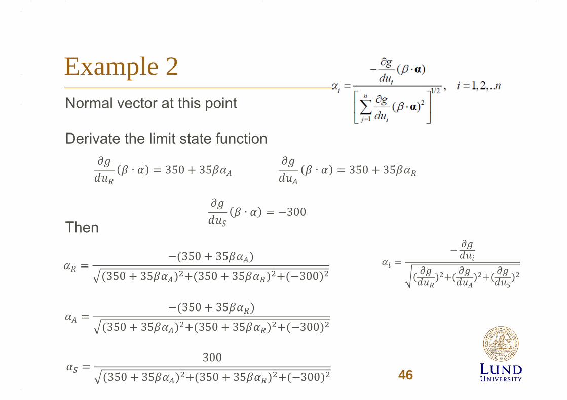
Example 2Normal vector at this point

Derivate the limit state function

Then

∙ 350 35 ∙ 350 35

∙ 300

350 35350 35 350 35 300

350 35350 35 350 35 300

300350 35 350 35 300 46

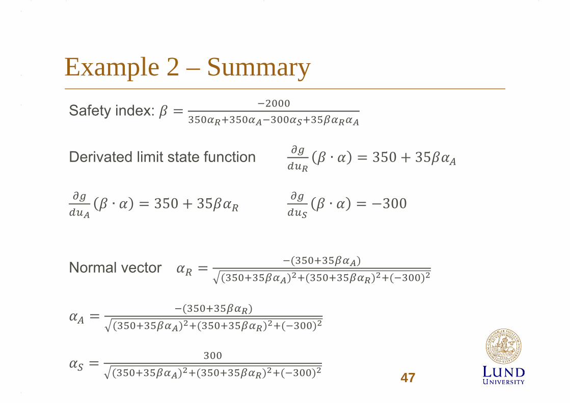
Example 2 – SummarySafety index:

Derivated limit state function ∙ 350 35

∙ 350 35 ∙ 300

Normal vector

47

Example 2 – Iteration

Safety index: 3.74

Start 1 2 3 4 5 6 7β 3 -3.9604 3.162993 3.764099 3.74638 3.744948 3.744835 3.744826αR 1 -0.64088 -0.63663 -0.56327 -0.56049 -0.56102 -0.56099 -0.561αA 1 -0.64088 -0.63663 -0.56327 -0.56049 -0.56102 -0.56099 -0.561αS 1 0.422556 0.435216 0.604532 0.609681 0.60869 0.608749 0.60874∂g/duR 455 438.8344 279.5224 275.7932 276.5072 276.4648 276.4712 276.4707∂g/duA 455 438.8344 279.5224 275.7932 276.5072 276.4648 276.4712 276.4707∂g/duS -300 -300 -300 -300 -300 -300 -300 -300

48

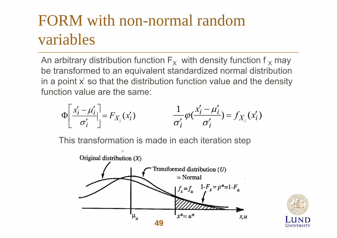
FORM with non-normal random variablesAn arbitrary distribution function FX with density function f X may be transformed to an equivalent standardized normal distribution in a point x so that the distribution function value and the density function value are the same:

)( iXi

ii xFxi

)()(1

iXi

ii

ixfx

i

This transformation is made in each iteration step

49

FORM with correlated, non-normal variables

The random variables are transformed to the U-space of uncorrelated and normalized variables. Two alternative methods may be used:

• The Rosenblatt transformation• The Nataf transformation

The education software COMREL uses the Rosenblatt transformation

50

Second order reliability method (SORM) • Is a more exact method since the expansion of the non-linear

limit state function also includes the second order derivatives of g(X)

FORM

SORMOriginal limit state function

51

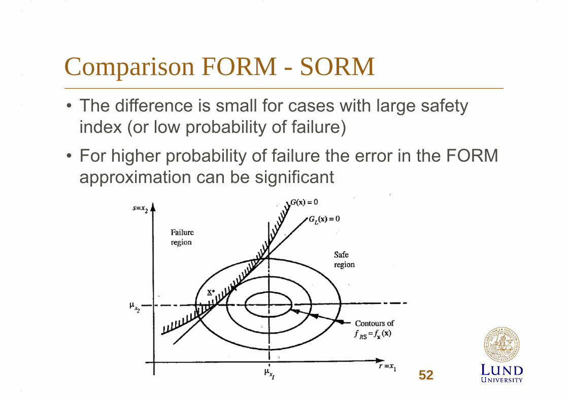
Comparison FORM - SORM• The difference is small for cases with large safety

index (or low probability of failure)• For higher probability of failure the error in the FORM

approximation can be significant

52

• Instead of calculating the reliability index, i.e. the failure probability analytically – it might be much easier to run virtual experiments based on the probabilistic models and the limit state function.

Monte Carlo Simulation

0

2

4

6

8

10

12

14

16

18

20

-2 0 2 4 6 8 10 12Load

Res

ista

nce

mn

p ff

Rand

om num

ber

1

)( iX xFi

jz

jx ix

Random outcome of X

53

Simulation methods

• Crude Monte Carlo simulation (simple but time consuming for low values of pf )

• Importance sampling• Directional simulation• Latin Hypercube simulation• Adaptive simulation methods

Simulation methods can also be used in the case of implicit limit state functions (e.g. FEM models)

54