pyscal DocumentationRelease 2.10.15

Sarath Menon, Grisell Díaz Leines, Jutta Rogal

Nov 06, 2021

CONTENTS

1 Highlights 3

2 Documentation 52.1 Download and Install . . . . . . . . . . . . . . . . . . . . . . . . . . . . . . . . . . . . . . . . . . . 52.2 News and updates . . . . . . . . . . . . . . . . . . . . . . . . . . . . . . . . . . . . . . . . . . . . 82.3 Methods and examples . . . . . . . . . . . . . . . . . . . . . . . . . . . . . . . . . . . . . . . . . . 82.4 pyscal reference . . . . . . . . . . . . . . . . . . . . . . . . . . . . . . . . . . . . . . . . . . . . . 602.5 Publications and Projects . . . . . . . . . . . . . . . . . . . . . . . . . . . . . . . . . . . . . . . . . 842.6 Support, contributing and extending . . . . . . . . . . . . . . . . . . . . . . . . . . . . . . . . . . . 852.7 Help and support . . . . . . . . . . . . . . . . . . . . . . . . . . . . . . . . . . . . . . . . . . . . . 862.8 Citing the code . . . . . . . . . . . . . . . . . . . . . . . . . . . . . . . . . . . . . . . . . . . . . . 862.9 Acknowledgements . . . . . . . . . . . . . . . . . . . . . . . . . . . . . . . . . . . . . . . . . . . . 872.10 License . . . . . . . . . . . . . . . . . . . . . . . . . . . . . . . . . . . . . . . . . . . . . . . . . . 87

Python Module Index 91

Index 93

i

ii

pyscal Documentation, Release 2.10.15

pyscal is a python module for the calculation of local atomic structural environments including Steinhardt’s bondorientational order parameters during post-processing of atomistic simulation data. The core functionality of pyscalis written in C++ with python wrappers using pybind11 which allows for fast calculations with possibilities for easyexpansion in python.

Steinhardt’s order parameters are widely used for identification of crystal structures. They are also used to identify ifan atom is solid or liquid. pyscal is inspired by BondOrderAnalysis code, but has since incorporated many additionsand modifications. pyscal module includes the following functionality-

CONTENTS 1

pyscal Documentation, Release 2.10.15

2 CONTENTS

CHAPTER

ONE

HIGHLIGHTS

• fast and efficient calculations using C++ and expansion using python.

• calculation of Steinhardt’s order parameters and their averaged version and disorder parameters.

• links with Voro++ code, for calculation of Steinhardt parameters weighted using face area of Voronoi polyhedra.

• classification of atoms as solid or liquid.

• clustering of particles based on a user defined property.

• methods for calculating radial distribution function, voronoi volume of particles, number of vertices and facearea of voronoi polyhedra and coordination number.

• calculation of angular parameters such as for identification of diamond structure and Ackland-Jones angularparameters.

• Centrosymmetry parameter for identification of defects.

• Adaptive common neighbor analysis for identification of crystal structures.

3

pyscal Documentation, Release 2.10.15

4 Chapter 1. Highlights

CHAPTER

TWO

DOCUMENTATION

2.1 Download and Install

2.1.1 Downloads

The source code is available in latest stable or release versions. We recommend using the latest stable version for allupdated features.

Source code

• latest stable version of pyscal (tar.gz)

• release version (zip)

Documentation

• PDF version

• Epub version

Publication

• Publication

• citation

2.1.2 Getting started

Trying pyscal

You can try some examples provided with pyscal using Binder without installing the package. Please use this link totry the package.

5

pyscal Documentation, Release 2.10.15

Installation

Supported operating systems

pyscal can be installed on Linux, Mac OS and Windows based systems.

Installation using conda

pyscal can be installed directly using Conda from the conda-forge channel by the following statement-

conda install -c conda-forge pyscal

This is the recommended way to install if you have an Anaconda distribution.

The above command installs the latest release version of pyscal and works on all three operating systems.

pyscal is no longer maintained for Python 2. Although quick installation method might␣→˓work for Python 2, all features may not work as expected.

Installation using pip

pyscal is not available on pip directly. However pyscal can be installed using pip by

pip install pybind11pip install git+https://github.com/pyscal/pyscal

Installation from the repository

pyscal can be built from the repository by-

git clone https://github.com/pyscal/pyscal.gitpip install pybind11cd pyscalpython setup.py install --user

Using a conda environment

pyscal can also be installed in a conda environment, making it easier to manage dependencies. A python3 Condaenvironment can be created by,

conda create -n myenv python=3

Once created, the environment can be activated using,

conda activate myenv

In case C++11 is not available, these can be installed using,

(myenv) conda install -c anaconda gcc

6 Chapter 2. Documentation

pyscal Documentation, Release 2.10.15

Now the pyscal repository can be cloned and the module can be installed. Python dependencies are installed automat-ically.

(myenv) git clone https://github.com/pyscal/pyscal.git(myenv) conda install -c conda-forge pybind11(myenv) cd pyscal(myenv) python setup.py install

A good guide on managing Conda environments is available[here](https://docs.conda.io/projects/conda/en/latest/user-guide/tasks/manage-→˓environments.html).

Dependencies

Dependencies for the C++ part

• pybind11

• C++ 11

Dependencies for the python part

• numpy

• ase

• plotly

• ipywidgets

Optional dependencies

• pytest

• matplotlib

• LAMMPS

Tests

In order to see if the installation worked, the following commands can be tried-

import pyscal.core as pcpc.test()

The above code does some minimal tests and gives a value of True if pyscal was installed successfully. However, pyscalalso contains automated tests which use the pytest python library, which can be installed by pip install pytest.The tests can be run by executing the command pytest tests/ from the main code directory.

It is good idea to run the tests to check if everything is installed properly.

2.1. Download and Install 7

pyscal Documentation, Release 2.10.15

2.2 News and updates

• November 21, 2019 pyscal is selected as the E-CAM module of the month. See the news here.

• November 1, 2019 pyscal paper is accepted in the Journal of Open Source Software. See the paper here.

• October 17, 2019 Publication for pyscal submitted to the Journal of Open Source Software. See the review here.

• July 12, 2019 Version 1.0.0 of pyscal is released.

2.3 Methods and examples

2.3.1 Methods

Methods to calculate neighbors of a particle

pyscal includes different methods to explore the local environment of a particle that rely on the calculation of nearestneighbors. Various approaches to compute the neighbors of particles are discussed here.

Fixed cutoff method

The most common method to calculate the nearest neighbors of an atom is using a cutoff radius. The neighborhoodof an atom for calculation of Steinhardt’s parameters {cite}``Steinhardt1983`` is often carried out using this method.Commonly, a cutoff is selected as the first minimum of the radial distribution functions. Once a cutoff is selected,the neighbors of an atom are those that fall within this selected radius. The following code snippet will use the cutoffmethod to calculate neighbors. In this example, conf.dump is assumed to be the input configuration of the system. Acutoff radius of 3 is assumed for calculation of neighbors.

import pyscal.core as pcsys = pc.System()sys.read_inputfile('conf.dump')sys.find_neighbors(method='cutoff', cutoff=3)

Adaptive cutoff methods

A fixed cutoff radius can introduce limitations to explore the local environment of the particle in some cases:

• At finite temperatures, when thermal fluctuations take place, the selection of a fixed cutoff may result in aninaccurate description of the local environment.

• If there is more than one structure present in the system, for example, bcc and fcc, the selection of cutoff suchthat it includes the first shell of both structures can be difficult.

In order to achieve a more accurate description of the local environment, various adaptive approaches have been pro-posed. Two of the methods implemented in the module are discussed below.

8 Chapter 2. Documentation

pyscal Documentation, Release 2.10.15

Solid angle based nearest neighbor algorithm (SANN)

SANN algorithm {cite}``VanMeel2012`` determines the cutoff radius by counting the solid angles around an atom andequating it to 4𝜋. The algorithm solves the following equation iteratively.

𝑅(𝑚)𝑖 =

∑𝑚𝑗=1 𝑟𝑖,𝑗

𝑚− 2< 𝑟𝑖,𝑚+1

where 𝑖 is the host atom, 𝑗 are its neighbors with 𝑟𝑖𝑗 is the distance between atoms 𝑖 and 𝑗. 𝑅𝑖 is the cutoff radius foreach particle 𝑖 which is found by increasing the neighbor of neighbors 𝑚 iteratively. For a description of the algorithmand more details, please check the reference {cite}``VanMeel2012``. SANN algorithm can be used to find the neighborsby,

import pyscal.core as pcsys = pc.System()sys.read_inputfile('conf.dump')sys.find_neighbors(method='cutoff', cutoff='sann')

Since SANN algorithm involves sorting, a sufficiently large cutoff is used in the beginning to reduce the number entriesto be sorted. This parameter is calculated by,

𝑟𝑖𝑛𝑖𝑡𝑖𝑎𝑙 = threshold ×(

Simulation box volume

Number of particles

) 13

a tunable threshold parameter can be set through function arguments.

Adaptive cutoff method

An adaptive cutoff specific for each atom can also be found using an algorithm similar to adaptive common neighboranalysis {cite}``Stukowski2012``. This adaptive cutoff is calculated by first making a list of all neighbor distances foreach atom similar to SANN method. Once this list is available, then the cutoff is calculated from,

𝑟𝑐𝑢𝑡(𝑖) = padding ×(

1

nlimit

nlimit∑𝑗=1

𝑟𝑖𝑗

)

This method can be chosen by,

import pyscal.core as pcsys = pc.System()sys.read_inputfile('conf.dump')sys.find_neighbors(method='cutoff', cutoff='adaptive')

The padding and nlimit parameters in the above equation can be tuned using the respective keywords.

Either of the adaptive method can be used to find neighbors, which can then be used to calculate Steinhardt’s parametersor their averaged version.

2.3. Methods and examples 9

pyscal Documentation, Release 2.10.15

Voronoi tessellation

Voronoi tessellation provides a completely parameter free geometric approach for calculation of neighbors. Voro++code is used for Voronoi tessellation. Neighbors can be calculated using this method by,

import pyscal.core as pcsys = pc.System()sys.read_inputfile('conf.dump')sys.find_neighbors(method='voronoi')

Finding neighbors using Voronoi tessellation also calculates a weight for each neighbor. The weight of a neighbor 𝑗towards a host atom 𝑖 is given by,

𝑊𝑖𝑗 =𝐴𝑖𝑗∑𝑁𝑗=1 𝐴𝑖𝑗

where 𝐴𝑖𝑗 is the area of Voronoi facet between atom 𝑖 and 𝑗, 𝑁 are all the neighbors identified through Voronoitessellation. This weight can be used later for calculation of weighted Steinhardt’s parameters. Optionally, it is possibleto choose the exponent for this weight. Option voroexp is used to set this option. For example if voroexp=2, theweight would be calculated as,

𝑊𝑖𝑗 =𝐴2

𝑖𝑗∑𝑁𝑗=1 𝐴

2𝑖𝑗

References

{bibliography} ../references.bib :filter: docname in docnames :style: unsrt

Steinhardt’s parameters

Steinhardt’s bond orientational order parameters {cite}``Steinhardt1983`` are a set of parameters based on spheri-cal harmonics to explore the local atomic environment. These parameters have been used extensively for varioususes such as distinction of crystal structures, identification of solid and liquid atoms and identification of defects{cite}``Steinhardt1983``.

These parameters, which are rotationally and translationally invariant are defined by,

𝑞𝑙(𝑖) =( 4𝜋

2𝑙 + 1

𝑙∑𝑚=−𝑙

|𝑞𝑙𝑚(𝑖)|2) 1

2

where,

𝑞𝑙𝑚(𝑖) =1

𝑁(𝑖)

𝑁(𝑖)∑𝑗=1

𝑌𝑙𝑚(𝑟𝑟𝑟𝑖𝑗)

10 Chapter 2. Documentation

pyscal Documentation, Release 2.10.15

in which 𝑌𝑙𝑚 are the spherical harmonics and𝑁(𝑖) is the number of neighbours of particle 𝑖, 𝑟𝑟𝑟𝑖𝑗 is the vector connectingparticles 𝑖 and 𝑗, and 𝑙 and 𝑚 are both intergers with 𝑚 ∈ [−𝑙,+𝑙]. Various parameters have found specific uses, suchas 𝑞2 and 𝑞6 for identification of crystallinity, 𝑞6 for identification of solidity, and 𝑞4 and 𝑞6 for distinction of crystalstructures {cite}``Mickel2013``. Commonly this method uses a cutoff radius to identify the neighbors of an atom. Thecutoff can be chosen based on different methods available. Once the cutoff is chosen and neighbors are calculated, thecalculation of Steinhardt’s parameters is straightforward.

sys.calculate_q([4, 6])q = sys.get_qvals([4, 6])

Averaged Steinhardt’s parameters

At high temperatures, thermal vibrations affect the atomic positions. This in turn leads to overlapping distributionsof 𝑞𝑙 parameters, which makes the identification of crystal structures difficult. To address this problem, the averagedversion 𝑞𝑙 of Steinhardt’s parameters was introduced by Lechner and Dellago {cite}``Lechner2008``. 𝑞𝑙 is given by,

𝑞𝑙(𝑖) =( 4𝜋

2𝑙 + 1

𝑙∑𝑚=−𝑙

1

��(𝑖)

��(𝑖)∑𝑘=0

𝑞𝑙𝑚(𝑘)2) 1

2

where the sum from 𝑘 = 0 to ��(𝑖) is over all the neighbors and the particle itself. The averaged parameters takesinto account the first neighbor shell and also information from the neighboring atoms and thus reduces the overlapbetween the distributions. Commonly 𝑞4 and 𝑞6 are used in identification of crystal structures. Averaged versions canbe calculated by setting the keyword averaged=True as follows.

sys.calculate_q([4, 6], averaged=True)q = sys.get_qvals([4, 6], averaged=True)

Voronoi weighted Steinhardt’s parameters

In order to improve the resolution of crystal structures Mickel et al {cite}``Mickel2013`` proposed weighting the con-tribution of each neighbor to the Steinhardt parameters by the ratio of the area of the Voronoi facet shared between theneighbor and host atom. The weighted parameters are given by,

𝑞𝑙𝑚(𝑖) =1

𝑁(𝑖)

𝑁(𝑖)∑𝑗=1

𝐴𝑖𝑗

𝐴𝑌𝑙𝑚(𝑟𝑟𝑟𝑖𝑗)

where 𝐴𝑖𝑗 is the area of the Voronoi facet between atoms 𝑖 and 𝑗 and 𝐴 is the sum of the face areas of atom 𝑖. Inpyscal, the area weights are already assigned during the neighbor calculation phase when the Voronoi method is usedto calculate neighbors in the System.find_neighbors. The Voronoi weighted Steinhardt’s parameters can be calculatedas follows,

sys.find_neighbors(method='voronoi')sys.calculate_q([4, 6])q = sys.get_qvals([4, 6])

The weighted Steinhardt’s parameters can also be averaged as described above. Once again, the keywordaveraged=True can be used for this purpose.

2.3. Methods and examples 11

pyscal Documentation, Release 2.10.15

sys.find_neighbors(method='voronoi')sys.calculate_q([4, 6], averaged=True)q = sys.get_qvals([4, 6], averaged=True)

It was also proposed that higher powers of the weight {cite}``Haeberle2019`` 𝐴𝛼𝑖𝑗

𝐴(𝛼) where 𝛼 = 2, 3 can also be used,where 𝐴(𝛼) =

∑𝑁(𝑖)𝑗=1 𝐴𝛼

𝑖𝑗 The value of this can be set using the keyword voroexp during the neighbor calculationphase.

sys.find_neighbors(method='voronoi', voroexp=2)

If the value of voroexp is set to 0, the neighbors would be found using Voronoi method, but the calculated Steinhardt’sparameters will not be weighted.

References

{bibliography} ../references.bib :filter: docname in docnames :style: unsrt

Classification of atoms as solid or liquid

pyscal can also be used to distinguish solid and liquid atoms. The classification is based on Steinhardt’s parame-ters, specifically 𝑞6. The method defines two neighboring atoms 𝑖 and 𝑗 as having solid bonds if a parameter 𝑠𝑖𝑗{cite}``Auer2005``,

𝑠𝑖𝑗 =

6∑𝑚=−6

𝑞6𝑚(𝑖)𝑞*6𝑚(𝑗) ≥ threshold

Additionally, a second order parameter is used to improve the distinction in solid-liquid boundaries{cite}``Bokeloh2014``. This is defined by the criteria,

⟨𝑠𝑖𝑗⟩ > avgthreshold

If a particle has 𝑛 number of bonds with 𝑠𝑖𝑗 ≥ threshold and the above condition is also satisfied, it is considered asa solid. The solid atoms can be clustered to find the largest solid cluster of atoms.

Finding solid atoms in liquid start with reading in a file and calculation of neighbors.

import pyscal.core as pcsys = pc.System()sys.read_inputfile('conf.dump')sys.find_neighbors(method='cutoff', cutoff=4)

Once again, there are various methods for finding neighbors. Please check here for details on neighbor calculationmethods. Once the neighbors are calculated, solid atoms can be found directly by,

sys.find_solids(bonds=6, threshold=0.5, avgthreshold=0.6, cluster=True)

bonds set the number of minimum bonds a particle should have (as defined above), threshold and avgthresholdare the same quantities that appear in the equations above. Setting the keyword cluster to True returns the size of thelargest solid cluster. It is also possible to check if each atom is solid or not.

12 Chapter 2. Documentation

pyscal Documentation, Release 2.10.15

atoms = sys.atomsolids = [atom.solid for atom in atoms]

References

{bibliography} ../references.bib :filter: docname in docnames :style: unsrt

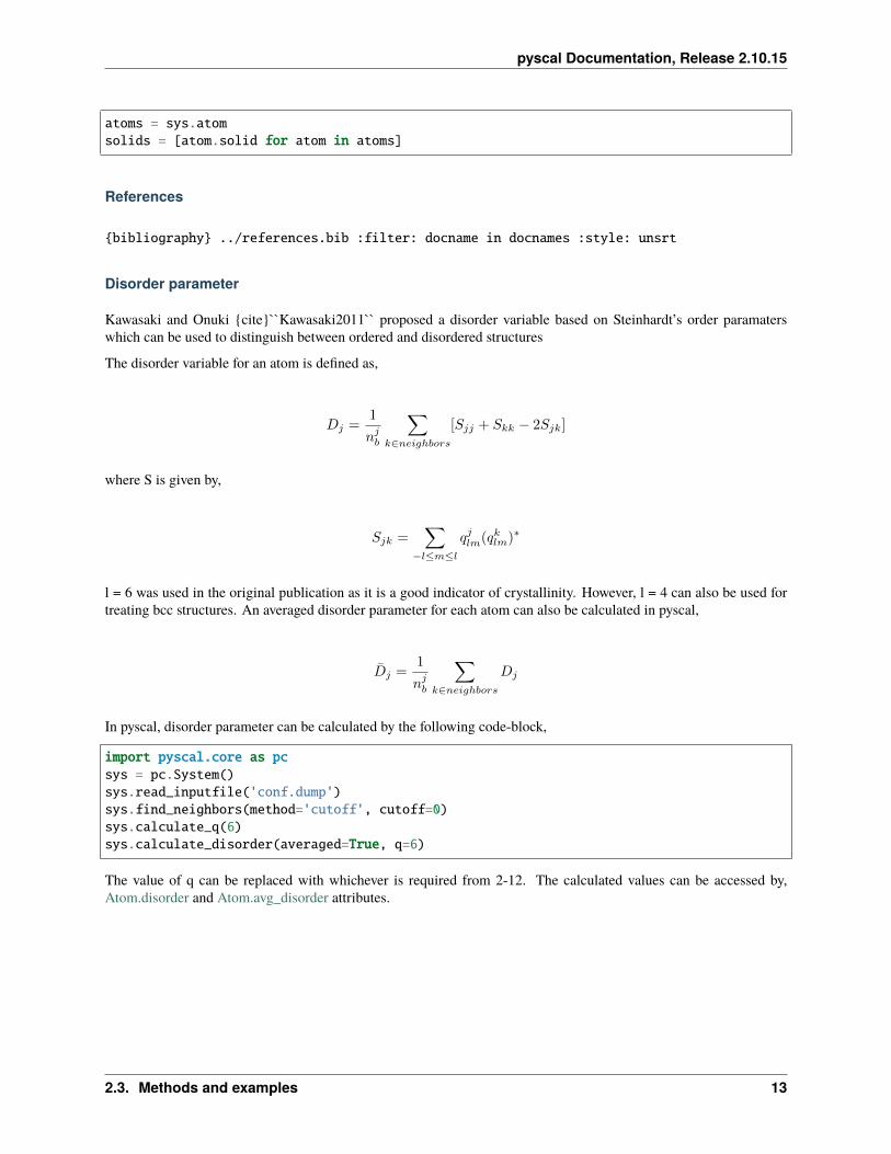
Disorder parameter

Kawasaki and Onuki {cite}``Kawasaki2011`` proposed a disorder variable based on Steinhardt’s order paramaterswhich can be used to distinguish between ordered and disordered structures

The disorder variable for an atom is defined as,

𝐷𝑗 =1

𝑛𝑗𝑏

∑𝑘∈𝑛𝑒𝑖𝑔ℎ𝑏𝑜𝑟𝑠

[𝑆𝑗𝑗 + 𝑆𝑘𝑘 − 2𝑆𝑗𝑘]

where S is given by,

𝑆𝑗𝑘 =∑

−𝑙≤𝑚≤𝑙

𝑞𝑗𝑙𝑚(𝑞𝑘𝑙𝑚)*

l = 6 was used in the original publication as it is a good indicator of crystallinity. However, l = 4 can also be used fortreating bcc structures. An averaged disorder parameter for each atom can also be calculated in pyscal,

��𝑗 =1

𝑛𝑗𝑏

∑𝑘∈𝑛𝑒𝑖𝑔ℎ𝑏𝑜𝑟𝑠

𝐷𝑗

In pyscal, disorder parameter can be calculated by the following code-block,

import pyscal.core as pcsys = pc.System()sys.read_inputfile('conf.dump')sys.find_neighbors(method='cutoff', cutoff=0)sys.calculate_q(6)sys.calculate_disorder(averaged=True, q=6)

The value of q can be replaced with whichever is required from 2-12. The calculated values can be accessed by,Atom.disorder and Atom.avg_disorder attributes.

2.3. Methods and examples 13

pyscal Documentation, Release 2.10.15

References

{bibliography} ../references.bib :filter: docname in docnames :style: unsrt

Angular parameters

Angular criteria for identification of diamond structure

Angular parameter introduced by Uttormark et al {cite}``Uttormark1993`` is used to measure the tetrahedrality of localatomic structure. An atom belonging to diamond structure has four nearest neighbors which gives rise to six three bodyangles around the atom. The angular parameter 𝐴 is then defined as,

𝐴 =

6∑𝑖=1

(cos(𝜃𝑖) +1

3)2

An atom belonging to diamond structure would show the value of angular params close to 0. Angular parameter canbe calculated in pyscal using the following method -

import pyscal.core as pcsys = pc.System()sys.read_inputfile('conf.dump')sys.find_neighbors(method='cutoff', cutoff='adaptive')sys.calculate_angularcriteria()

The calculated angular criteria value can be accessed for each atom using Atom.angular.

𝜒 parameters for structural identification

𝜒 parameters introduced by Ackland and Jones {cite}``Ackland2006`` measures all local angles created by an atom withits neighbors and creates a histogram of these angles to produce vector which can be used to identify structures. Afterfinding the neighbors of an atom, cos 𝜃𝑖𝑗𝑘 for atoms j and k which are neighbors of i is calculated for all combinationsof i, j and k. The set of all calculated cosine values are then added to a histogram with the following bins - [-1.0, -0.945,-0.915, -0.755, -0.705, -0.195, 0.195, 0.245, 0.795, 1.0]. Compared to 𝜒 parameters from 𝜒0 to 𝜒7 in the associatedpublication, the vector calculated in pyscal contains values from 𝜒0 to 𝜒8 which is due to an additional 𝜒 parameterwhich measures the number of neighbors between cosines -0.705 to -0.195. The 𝜒 vector is characteristic of the localatomic environment and can be used to identify crystal structures, details of which can be found in the publication[^2].

𝜒 parameters can be calculated in pyscal using,

import pyscal.core as pcsys = pc.System()sys.read_inputfile('conf.dump')sys.find_neighbors(method='cutoff', cutoff='adaptive')sys.calculate_chiparams()

The calculated values for each atom can be accessed using Atom.chiparams.

14 Chapter 2. Documentation

pyscal Documentation, Release 2.10.15

References

{bibliography} ../references.bib :filter: docname in docnames :style: unsrt

Voronoi tessellation to identify local structures

Voronoi tessellation can be used for identification of local structure by counting the number of faces of the Voronoipolyhedra of an atom {cite}``Finney1970,Tanemura1977``. For each atom a vector ⟨𝑛3 𝑛4 𝑛5 𝑛6⟩ can be calculatedwhere 𝑛3 is the number of Voronoi faces of the associated Voronoi polyhedron with three vertices, 𝑛4 is with fourvertices and so on. Each perfect crystal structure such as a signature vector, for example, bcc can be identified by⟨0 6 0 8⟩ and fcc can be identified using ⟨0 12 0 0⟩. It is also a useful tool for identifying icosahedral structure whichhas the fingerprint ⟨0 0 12 0⟩. In pyscal, the voronoi vector can be calculated using,

import pyscal.core as pcsys = pc.System()sys.read_inputfile('conf.dump')sys.find_neighbors(method='voronoi')sys.calculate_vorovector()

The vector for each atom can be accessed using Atom.vorovector. Furthermore, the associated Voronoi volume of thepolyhedron, which may be indicative of the local structure, is also automatically calculated when finding neighborsusing System.find_neighbors. This value for each atom can be accessed by Atom.volume. An averaged version of thevolume, which is averaged over the neighbors of an atom can be accessed using Atom.avg_volume.

References

{bibliography} ../references.bib :filter: docname in docnames :style: unsrt

Centrosymmetry parameter

Centrosymmetry parameter (CSP) was introduced by Kelchner et al. {cite}``Kelchner1998`` to identify defects incrystals. The parameter measures the loss of local symmetry. For an atom with 𝑁 nearest neighbors, the parameter isgiven by,

CSP =

𝑁/2∑𝑖=1

r𝑖 + r𝑖+𝑁/2

2r𝑖 and r𝑖+𝑁/2 are vectors from the central atom to two opposite pairs of neighbors. There are two main methods toidentify the opposite pairs of neighbors as described in this publication. The first of the approaches is called GreedyEdge Selection (GES) {cite}``Stukowski2012`` and is implemented in LAMMPS and Ovito. GES algorithm calculatesa weight 𝑤𝑖𝑗 = |r𝑖 + r𝑗 | for all combinations of neighbors around an atom and calculates CSP over the smallest 𝑁/2weights.

A centrosymmetry parameter calculation using GES algorithm can be carried out as follows-

import pyscal.core as pcsys = pc.System()sys.read_inputfile('conf.dump')sys.find_neighbors(method='voronoi')sys.calculate_centrosymmetry(nmax = 12)

2.3. Methods and examples 15

pyscal Documentation, Release 2.10.15

nmax parameter specifies the number of nearest neighbors to be considered for the calculation of CSP. The secondalgorithm is called the Greedy Vertex Matching {cite}``Bulatov2006`` and is implemented in AtomEye and Atomsk.This algorithm orders the neighbors atoms in order of increasing distance from the central atom. From this list, theclosest neighbor is paired with its lowest weight partner and both atoms removed from the list. This process is continueduntil no more atoms are remaining in the list. CSP calculation using this algorithm can be carried out by,

import pyscal.core as pcsys = pc.System()sys.read_inputfile('conf.dump')sys.find_neighbors(method='voronoi')sys.calculate_centrosymmetry(nmax = 12, algorithm = "gvm")

References

{bibliography} ../references.bib :filter: docname in docnames :style: unsrt

Entropy - Enthalpy parameters

Entropy fingerprint

The entropy parameter was introduced by Piaggi et al {cite}``Piaggi2017`` for identification of defects and distinctionbetween solid and liquid. The entropy paramater 𝑠𝑖𝑠 is defined as,

𝑠𝑖𝑠 = −2𝜋𝜌𝑘𝐵

∫ 𝑟𝑚

0

[𝑔𝑖𝑚(𝑟) ln 𝑔𝑖𝑚(𝑟) − 𝑔𝑖𝑚(𝑟) + 1]𝑟2𝑑𝑟

where 𝑟𝑚 is the upper bound of integration and 𝑔𝑖𝑚 is radial distribution function centered on atom 𝑖,

𝑔𝑖𝑚(𝑟) =1

4𝜋𝜌𝑟2

∑𝑗

1√2𝜋𝜎2

exp−(𝑟 − 𝑟𝑖𝑗)2/(2𝜎2)

𝑟𝑖𝑗 is the interatomic distance between atom 𝑖 and its neighbors 𝑗 and 𝜎 is a broadening parameter.

The averaged version of entropy parameters 𝑠𝑖𝑠 can be calculated in two ways, either using a simple averaging over theneighbors given by,

𝑠𝑖𝑠 =

∑𝑗 𝑠

𝑗𝑠 + 𝑠𝑖𝑠

𝑁 + 1

or using a switching function as described below,

𝑠𝑖𝑠 =

∑𝑗 𝑠

𝑖𝑠𝑓(𝑟𝑖𝑗) + 𝑠𝑖𝑠∑

𝑗 𝑓(𝑟𝑖𝑗) + 1

𝑓(𝑟𝑖𝑗) is a switching parameter which depends on 𝑟𝑎 which is the cutoff distance. The switching function shows avalue of 1 for 𝑟𝑖𝑗 << 𝑟𝑎 and 0 for 𝑟𝑖𝑗 >> 𝑟𝑎. The switching function is given by,

16 Chapter 2. Documentation

pyscal Documentation, Release 2.10.15

𝑓(𝑟𝑖𝑗) =1 − (𝑟𝑖𝑗/𝑟𝑎)𝑁

1 − (𝑟𝑖𝑗/𝑟𝑎)𝑀

Entropy parameters can be calculated in pyscal using the following code,

import pyscal.core as pcsys = pc.System()sys.read_inputfile('conf.dump')sys.find_neighbors(method="cutoff", cutoff=0)lattice_constant=4.00sys.calculate_entropy(1.4*lattice_constant, averaged=True)atoms = sys.atomsentropy = [atom.entropy for atom in atoms]average_entropy = [atom.avg_entropy for atom in atoms]

The value of 𝑟𝑚 is provided in units of lattice constant. Further parameters shown above, such as 𝜎 can be specifiedusing the various keyword arguments. The above code does a simple averaging over neighbors. The switching functioncan be used by,

sys.calculate_entropy(1.4*lattice_constant, ra=0.9*lattice_constant, switching_→˓function=True, averaged=True)

In pyscal, a slightly different version of 𝑠𝑖𝑠 is calculated. This is given by,

𝑠𝑖𝑠 = −𝜌

∫ 𝑟𝑚

0

[𝑔𝑖𝑚(𝑟) ln 𝑔𝑖𝑚(𝑟) − 𝑔𝑖𝑚(𝑟) + 1]𝑟2𝑑𝑟

The prefactor 2𝜋𝑘𝐵 is dropped in the entropy values calculated in pyscal.

References

{bibliography} ../references.bib :filter: docname in docnames :style: unsrt

2.3.2 Examples

Getting started with pyscal

This example illustrates basic functionality of pyscal python library by setting up a system and the atoms.

[1]: import pyscal as pcimport numpy as np

2.3. Methods and examples 17

pyscal Documentation, Release 2.10.15

The System class

System is the basic class of pyscal and is required to be setup in order to perform any calculations. It can be set up as-

[2]: sys = pc.System()

sys is a System object. But at this point, it is completely empty. We have to provide the system with the followinginformation- * the simulation box dimensions * the positions of individual atoms.

Let us try to set up a small system, which is the bcc unitcell of lattice constant 1. The simulation box dimensions ofsuch a unit cell would be [[0.0, 1.0], [0.0, 1.0], [0.0, 1.0]] where the first set correspond to the x axis, second to y axisand so on.The unitcell has 2 atoms and their positions are [0,0,0] and [0.5, 0.5, 0.5].

[4]: sys.box = [[1.0, 0.0, 0.0], [0.0, 1.0, 0.0], [0.0, 0.0, 1.0]]

We can easily check if everything worked by getting the box dimensions

[5]: sys.box

[5]: [[1.0, 0.0, 0.0], [0.0, 1.0, 0.0], [0.0, 0.0, 1.0]]

The Atom class

The next part is assigning the atoms. This can be done using the Atom class. Here, we will only look at the basicproperties of Atom class. For a more detailed description, check the examples.Now let us create two atoms.

[6]: atom1 = pc.Atom()atom2 = pc.Atom()

Now two empty atom objects are created. The basic poperties of an atom are its positions and id. There are variousother properties which can be set here. A detailed description can be found here.

[7]: atom1.pos = [0., 0., 0.]atom1.id = 0atom2.pos = [0.5, 0.5, 0.5]atom2.id = 1

Alternatively, atom objects can also be set up as

[8]: atom1 = pc.Atom(pos=[0., 0., 0.], id=0)atom2 = pc.Atom(pos=[0.5, 0.5, 0.5], id=1)

We can check the details of the atom by querying it

[9]: atom1.pos

[9]: [0.0, 0.0, 0.0]

18 Chapter 2. Documentation

pyscal Documentation, Release 2.10.15

Combining System and Atom

Now that we have created the atoms, we can assign them to the system. We can also assign the same box we createdbefore.

[10]: sys = pc.System()sys.box = [[1.0, 0.0, 0.0], [0.0, 1.0, 0.0], [0.0, 0.0, 1.0]]sys.atoms = [atom1, atom2]

That sets up the system completely. It has both of it’s constituents - atoms and the simulation box. We can check ifeverything works correctly.

[11]: sys.atoms

[11]: [<pyscal.catom.Atom at 0x7f66e9752730>, <pyscal.catom.Atom at 0x7f66e9752930>]

This returns all the atoms of the system. Alternatively a single atom can be accessed by,

[12]: atom = sys.get_atom(1)

The above call will fetch the atom at position 1 in the list of all atoms in the system. Due to Atom being a completelyC++ class, it is necessary to use get_atom() and set_atom() to access individual atoms and set them back into thesystem object after modification. A list of all atoms however can be accessed directly by atoms.

Once you have all the atoms, you can modify any one and add it back to the list of all atoms in the system. The followingstatement will set the type of the first atom to 2.

[13]: atom = sys.atoms[0]atom.type = 2

Lets verify if it was done properly

[14]: atom.type

[14]: 2

Now we can push the atom back to the system with the new type

[15]: sys.set_atom(atom)

Reading in an input file

We are all set! The System is ready for calculations. However, in most realistic simulation situations, we have manyatoms and it can be difficult to set each of themindividually. In this situation we can read in input file directly. An example input file containing 500 atoms in asimulation box can be read in automatically. The file we use for this example is a file of the lammps-dump format.pyscal can also read in POSCAR files. In principle, pyscal only needs the atom positions and simulation box size,so you can write a python function to process the input file, extract the details and pass to pyscal.

[16]: sys = pc.System()sys.read_inputfile('conf.dump')

Once again, lets check if the box dimensions are read in correctly

2.3. Methods and examples 19

pyscal Documentation, Release 2.10.15

[17]: sys.box

[17]: [[18.85618, 0.0, 0.0], [0.0, 18.86225, 0.0], [0.0, 0.0, 19.01117]]

Now we can get all atoms that belong to this system

[18]: len(sys.atoms)

[18]: 500

We can see that all the atoms are read in correctly and there are 500 atoms in total. Once again, individual atomproperties can beaccessed as before.

[19]: sys.atoms[0].pos

[19]: [-5.66782, -6.06781, -6.58151]

Thats it! Now we are ready for some calculations. You can find more in the examples section of the documentation.

Calculating coordination numbers

In this example, we will read in a configuration from an MD simulation and then calculate the coordination numberdistribution.This example assumes that you read the basic example.

[1]: import pyscal as pcimport numpy as npimport matplotlib.pyplot as plt

Read in a file

The first step is setting up a system. We can create atoms and simulation box using the pyscal.crystal_structuresmodule. Let us start by importing the module.

[2]: import pyscal.crystal_structures as pcs

[3]: atoms, box = pcs.make_crystal('bcc', lattice_constant= 4.00, repetitions=[6,6,6])

The above function creates an bcc crystal of 6x6x6 unit cells with a lattice constant of 4.00 along with a simulation boxthat encloses the particles. We can then create a System and assign the atoms and box to it.

[4]: sys = pc.System()sys.box = boxsys.atoms = atoms

20 Chapter 2. Documentation

pyscal Documentation, Release 2.10.15

Calculating neighbors

We start by calculating the neighbors of each atom in the system. There are two ways to do this, using a cutoff methodand using a voronoi polyhedra method. We will try with both of them. First we try with cutoff system - which hasthree sub options. We will check each of them in detail.

Cutoff method

Cutoff method takes cutoff distance value and finds all atoms within the cutoff distance of the host atom.

[5]: sys.find_neighbors(method='cutoff', cutoff=4.1)

Now lets get all the atoms.

[6]: atoms = sys.atoms

let us try accessing the coordination number of an atom

[7]: atoms[0].coordination

[7]: 14

As we would expect for a bcc type lattice, we see that the atom has 14 neighbors (8 in the first shell and 6 in the second).Lets try a more interesting example by reading in a bcc system with thermal vibrations. Thermal vibrations lead todistortion in atomic positions, and hence there will be a distribution of coordination numbers.

[8]: sys = pc.System()sys.read_inputfile('conf.dump')sys.find_neighbors(method='cutoff', cutoff=3.6)atoms = sys.atoms

We can loop over all atoms and create a histogram of the results

[9]: coord = [atom.coordination for atom in atoms]

Now lets plot and see the results

[10]: nos, counts = np.unique(coord, return_counts=True)plt.bar(nos, counts, color="#AD1457")plt.ylabel("density")plt.xlabel("coordination number")plt.title("Cutoff method")

[10]: Text(0.5, 1.0, 'Cutoff method')

2.3. Methods and examples 21

pyscal Documentation, Release 2.10.15

Adaptive cutoff methods

pyscal also has adaptive cutoff methods implemented. These methods remove the restriction on having the samecutoff. A distinct cutoff is selected for each atom during runtime. pyscal uses two distinct algorithms to do this -sann and adaptive. Please check the documentation for a explanation of these algorithms. For the purpose of thisexample, we will use the adaptive algorithm.

adaptive algorithm

[11]: sys.find_neighbors(method='cutoff', cutoff='adaptive', padding=1.5)atoms = sys.atomscoord = [atom.coordination for atom in atoms]

Now lets plot

[12]: nos, counts = np.unique(coord, return_counts=True)plt.bar(nos, counts, color="#AD1457")plt.ylabel("density")plt.xlabel("coordination number")plt.title("Cutoff adaptive method")

[12]: Text(0.5, 1.0, 'Cutoff adaptive method')

22 Chapter 2. Documentation

pyscal Documentation, Release 2.10.15

The adaptive method also gives similar results!

Voronoi method

Voronoi method calculates the voronoi polyhedra of all atoms. Any atom that shares a voronoi face area with the hostatom are considered neighbors. Voronoi polyhedra is calculated using the Voro++ code. However, you dont need toinstall this specifically as it is linked to pyscal.

[13]: sys.find_neighbors(method='voronoi')

Once again, let us get all atoms and find their coordination

[14]: atoms = sys.atomscoord = [atom.coordination for atom in atoms]

And visualise the results

[15]: nos, counts = np.unique(coord, return_counts=True)plt.bar(nos, counts, color="#AD1457")plt.ylabel("density")plt.xlabel("coordination number")plt.title("Voronoi method")

[15]: Text(0.5, 1.0, 'Voronoi method')

2.3. Methods and examples 23

pyscal Documentation, Release 2.10.15

Finally..

All methods find the coordination number, and the results are comparable. Cutoff method is very sensitive to the choiceof cutoff radius, but voronoi method can slightly overestimate the neighbors due to thermal vibrations.

Calculating bond orientational order parameters

This example illustrates the calculation of bond orientational order parameters. Bond order parameters, 𝑞𝑙 and theiraveraged versions, 𝑞𝑙 are widely used to identify atoms belong to different crystal structures. In this example, we willconsider bcc, fcc, and hcp, and calculate the 𝑞4 and 𝑞6 parameters and their averaged versions which are widely usedin literature. More details can be found here.

[1]: import pyscal as pcimport pyscal.crystal_structures as pcsimport numpy as npimport matplotlib.pyplot as plt

In this example, we analyse MD configurations, first a set of perfect bcc, fcc and hcp structures and another set withthermal vibrations.

Perfect structures

To create atoms and box for perfect structures, the :mod:~pyscal.crystal_structuresmodule is used. The createdatoms and boxes are then assigned to System objects.

[2]: bcc_atoms, bcc_box = pcs.make_crystal('bcc', lattice_constant=3.147, repetitions=[4,4,4])bcc = pc.System()bcc.box = bcc_boxbcc.atoms = bcc_atoms

24 Chapter 2. Documentation

pyscal Documentation, Release 2.10.15

[3]: fcc_atoms, fcc_box = pcs.make_crystal('fcc', lattice_constant=3.147, repetitions=[4,4,4])fcc = pc.System()fcc.box = fcc_boxfcc.atoms = fcc_atoms

[4]: hcp_atoms, hcp_box = pcs.make_crystal('hcp', lattice_constant=3.147, repetitions=[4,4,4])hcp = pc.System()hcp.box = hcp_boxhcp.atoms = hcp_atoms

Next step is calculation of nearest neighbors. There are two ways to calculate neighbors, by using a cutoff distanceor by using the voronoi cells. In this example, we will use the cutoff method and provide a cutoff distance for eachstructure.

Finding the cutoff distance

The cutoff distance is normally calculated in a such a way that the atoms within the first shell is incorporated in thisdistance. The :func:pyscal.core.System.calculate_rdf function can be used to find this cutoff distance.

[5]: bccrdf = bcc.calculate_rdf()fccrdf = fcc.calculate_rdf()hcprdf = hcp.calculate_rdf()

Now the calculated rdf is plotted

[6]: fig, (ax1, ax2, ax3) = plt.subplots(1, 3, figsize=(11,4))ax1.plot(bccrdf[1], bccrdf[0])ax2.plot(fccrdf[1], fccrdf[0])ax3.plot(hcprdf[1], hcprdf[0])ax1.set_xlim(0,5)ax2.set_xlim(0,5)ax3.set_xlim(0,5)ax1.set_title('bcc')ax2.set_title('fcc')ax3.set_title('hcp')ax2.set_xlabel("distance")ax1.axvline(3.6, color='red')ax2.axvline(2.7, color='red')ax3.axvline(3.6, color='red')

[6]: <matplotlib.lines.Line2D at 0x7f7319324978>

2.3. Methods and examples 25

pyscal Documentation, Release 2.10.15

The selected cutoff distances are marked in red in the above plot. For bcc, since the first two shells are close to eachother, for this example, we will take the cutoff in such a way that both shells are included.

Steinhardt’s parameters - cutoff neighbor method

[7]: bcc.find_neighbors(method='cutoff', cutoff=3.6)fcc.find_neighbors(method='cutoff', cutoff=2.7)hcp.find_neighbors(method='cutoff', cutoff=3.6)

We have used a cutoff of 3 here, but this is a parameter that has to be tuned. Using a different cutoff for each structureis possible, but it would complicate the method if the system has a mix of structures. Now we can calculate the 𝑞4 and𝑞6 distributions

[8]: bcc.calculate_q([4,6])fcc.calculate_q([4,6])hcp.calculate_q([4,6])

Thats it! Now lets gather the results and plot them.

[9]: bccq = bcc.get_qvals([4, 6])fccq = fcc.get_qvals([4, 6])hcpq = hcp.get_qvals([4, 6])

[10]: plt.scatter(bccq[0], bccq[1], s=60, label='bcc', color='#C62828')plt.scatter(fccq[0], fccq[1], s=60, label='fcc', color='#FFB300')plt.scatter(hcpq[0], hcpq[1], s=60, label='hcp', color='#388E3C')plt.xlabel("$q_4$", fontsize=20)plt.ylabel("$q_6$", fontsize=20)plt.legend(loc=4, fontsize=15)

[10]: <matplotlib.legend.Legend at 0x7f7319202160>

26 Chapter 2. Documentation

pyscal Documentation, Release 2.10.15

Firstly, we can see that Steinhardt parameter values of all the atoms fall on one specific point which is due to theabsence of thermal vibrations. Next, all the points are well separated and show good distinction. However, at finitetemperatures, the atomic positions are affected by thermal vibrations and hence show a spread in the distribution. Wewill show the effect of thermal vibrations in the next example.

Structures with thermal vibrations

Once again, we create the reqd structures using the :mod:~pyscal.crystal_structures module. Noise can beapplied to atomic positions using the noise keyword as shown below.

[11]: bcc_atoms, bcc_box = pcs.make_crystal('bcc', lattice_constant=3.147, repetitions=[10,10,→˓10], noise=0.1)bcc = pc.System()bcc.box = bcc_boxbcc.atoms = bcc_atoms

[12]: fcc_atoms, fcc_box = pcs.make_crystal('fcc', lattice_constant=3.147, repetitions=[10,10,→˓10], noise=0.1)fcc = pc.System()fcc.box = fcc_boxfcc.atoms = fcc_atoms

[13]: hcp_atoms, hcp_box = pcs.make_crystal('hcp', lattice_constant=3.147, repetitions=[10,10,→˓10], noise=0.1)hcp = pc.System()hcp.box = hcp_boxhcp.atoms = hcp_atoms

2.3. Methods and examples 27

pyscal Documentation, Release 2.10.15

cutoff method

[14]: bcc.find_neighbors(method='cutoff', cutoff=3.6)fcc.find_neighbors(method='cutoff', cutoff=2.7)hcp.find_neighbors(method='cutoff', cutoff=3.6)

And now, calculate 𝑞4, 𝑞6 parameters

[15]: bcc.calculate_q([4,6])fcc.calculate_q([4,6])hcp.calculate_q([4,6])

Gather the q vales and plot them

[16]: bccq = bcc.get_qvals([4, 6])fccq = fcc.get_qvals([4, 6])hcpq = hcp.get_qvals([4, 6])

[17]: plt.scatter(fccq[0], fccq[1], s=10, label='fcc', color='#FFB300')plt.scatter(hcpq[0], hcpq[1], s=10, label='hcp', color='#388E3C')plt.scatter(bccq[0], bccq[1], s=10, label='bcc', color='#C62828')plt.xlabel("$q_4$", fontsize=20)plt.ylabel("$q_6$", fontsize=20)plt.legend(loc=4, fontsize=15)

[17]: <matplotlib.legend.Legend at 0x7f7318e60e80>

The thermal vibrations cause the distributions to spread, but it still very good. Lechner and Dellago proposed usingthe averaged distributions, 𝑞4 − 𝑞6 to better distinguish the distributions. Lets try that.

[18]: bcc.calculate_q([4,6], averaged=True)fcc.calculate_q([4,6], averaged=True)hcp.calculate_q([4,6], averaged=True)

[19]: bccaq = bcc.get_qvals([4, 6], averaged=True)fccaq = fcc.get_qvals([4, 6], averaged=True)

(continues on next page)

28 Chapter 2. Documentation

pyscal Documentation, Release 2.10.15

(continued from previous page)

hcpaq = hcp.get_qvals([4, 6], averaged=True)

Lets see if these distributions are better..

[20]: plt.scatter(fccaq[0], fccaq[1], s=10, label='fcc', color='#FFB300')plt.scatter(hcpaq[0], hcpaq[1], s=10, label='hcp', color='#388E3C')plt.scatter(bccaq[0], bccaq[1], s=10, label='bcc', color='#C62828')plt.xlabel("$q_4$", fontsize=20)plt.ylabel("$q_6$", fontsize=20)plt.legend(loc=4, fontsize=15)

[20]: <matplotlib.legend.Legend at 0x7f7318d640f0>

This looks much better! We can see that the resolution is much better than the non averaged versions.

There is also the possibility to calculate structures using Voronoi based neighbor identification too. Let’s try that now.

[21]: bcc.find_neighbors(method='voronoi')fcc.find_neighbors(method='voronoi')hcp.find_neighbors(method='voronoi')

[22]: bcc.calculate_q([4,6], averaged=True)fcc.calculate_q([4,6], averaged=True)hcp.calculate_q([4,6], averaged=True)

[23]: bccaq = bcc.get_qvals([4, 6], averaged=True)fccaq = fcc.get_qvals([4, 6], averaged=True)hcpaq = hcp.get_qvals([4, 6], averaged=True)

Plot the calculated points..

[24]: plt.scatter(fccaq[0], fccaq[1], s=10, label='fcc', color='#FFB300')plt.scatter(hcpaq[0], hcpaq[1], s=10, label='hcp', color='#388E3C')plt.scatter(bccaq[0], bccaq[1], s=10, label='bcc', color='#C62828')plt.xlabel("$q_4$", fontsize=20)

(continues on next page)

2.3. Methods and examples 29

pyscal Documentation, Release 2.10.15

(continued from previous page)

plt.ylabel("$q_6$", fontsize=20)plt.legend(loc=4, fontsize=15)

[24]: <matplotlib.legend.Legend at 0x7f7318dfaba8>

Voronoi based method also provides good resolution,the major difference being that the location of bcc distribution isdifferent.

Analyzing a lammps trajectory

In this example, a lammps trajectory in dump-text format will be read in, and Steinhardt’s parameters will be calculated.

[1]: import pyscal as pcimport osimport pyscal.traj_process as ptpimport matplotlib.pyplot as pltimport numpy as np

First, we will use the split_trajectory method from pyscal.traj_process module to help split the trajectoryinto individual snapshots.

[2]: trajfile = "traj.light"files = ptp.split_trajectory(trajfile)

files contain the individual time slices from the trajectory.

[3]: len(files)

[3]: 10

[4]: files[0]

[4]: 'traj.light.snap.0.dat'

Now we can make a small function which reads a single configuration and calculates 𝑞6 values.

30 Chapter 2. Documentation

pyscal Documentation, Release 2.10.15

[5]: def calculate_q6(file, format="lammps-dump"):sys = pc.System()sys.read_inputfile(file, format=format)sys.find_neighbors(method="cutoff", cutoff=0)sys.calculate_q(6)q6 = sys.get_qvals(6)return q6

There are a couple of things of interest in the above function. The find_neighbors method finds the neighbors of theindividual atoms. Here, an adaptive method is used, but, one can also use a fixed cutoff or Voronoi tessellation. Alsoonly the unaveraged 𝑞6 values are calculated above. The averaged ones can be calculate using the averaged=Truekeyword in both calculate_q and get_qvals method. Now we can simply call the function for each file..

[6]: q6s = [calculate_q6(file) for file in files]

We can now visualise the calculated values

[7]: plt.plot(np.hstack(q6s))

[7]: [<matplotlib.lines.Line2D at 0x7f5e424c0f60>]

Adding a clustering condition

We will now modify the above function to also find clusters which satisfy particular 𝑞6 value. But first, for a single file.

[8]: sys = pc.System()sys.read_inputfile(files[0])sys.find_neighbors(method="cutoff", cutoff=0)sys.calculate_q(6)

Now a clustering algorithm can be applied on top using the cluster_atoms method. cluster_atoms uses acondition as argument which should give a True/False value for each atom. Lets define a condition.

[9]: def condition(atom):return atom.get_q(6) > 0.5

2.3. Methods and examples 31

pyscal Documentation, Release 2.10.15

The above function returns True for any atom which has a 𝑞6 value greater than 0.5 and False otherwise. Now wecan call the cluster_atoms method.

[10]: sys.cluster_atoms(condition)

[10]: 16

The method returns 16, which here is the size of the largest cluster of atoms which have 𝑞6 value of 0.5 or higher. Ifinformation about all clusters are required, that can also be accessed.

[11]: atoms = sys.atoms

atom.cluster gives the number of the cluster that each atom belongs to. If the value is -1, the atom does not belongto any cluster, that is, the clustering condition was not met.

[12]: clusters = [atom.cluster for atom in atoms if atom.cluster != -1]

Now we can see how many unique clusters are there, and what their sizes are.

[13]: unique_clusters, counts = np.unique(clusters, return_counts=True)

counts contain all the necessary information. len(counts) will give the number of unique clusters.

[14]: plt.bar(range(len(counts)), counts)plt.ylabel("Number of atoms in cluster")plt.xlabel("Cluster ID")

[14]: Text(0.5, 0, 'Cluster ID')

Now we can finally put all of these together into a single function and run it over our individual time slices.

[15]: def calculate_q6_cluster(file, cutoff_q6 = 0.5, format="lammps-dump"):sys = pc.System()sys.read_inputfile(file, format=format)sys.find_neighbors(method="cutoff", cutoff=0)sys.calculate_q(6)def _condition(atom):

return atom.get_q(6) > cutoff_q6(continues on next page)

32 Chapter 2. Documentation

pyscal Documentation, Release 2.10.15

(continued from previous page)

sys.cluster_atoms(condition)atoms = sys.atomsclusters = [atom.cluster for atom in atoms if atom.cluster != -1]unique_clusters, counts = np.unique(clusters, return_counts=True)return counts

[16]: q6clusters = [calculate_q6_cluster(file) for file in files]

We can plot the number of clusters for each slice

[17]: plt.plot(range(len(q6clusters)), [len(x) for x in q6clusters], 'o-')plt.xlabel("Time slice")plt.ylabel("number of unique clusters")

[17]: Text(0, 0.5, 'number of unique clusters')

We can also plot the biggest cluster size

[18]: plt.plot(range(len(q6clusters)), [max(x) for x in q6clusters], 'o-')plt.xlabel("Time slice")plt.ylabel("Largest cluster size")

[18]: Text(0, 0.5, 'Largest cluster size')

2.3. Methods and examples 33

pyscal Documentation, Release 2.10.15

The final thing to do is to remove the split files after use.

[19]: for file in files:os.remove(file)

Using ASE

The above example can also done using ASE. The ASE read method needs to be imported.

[20]: from ase.io import read

[21]: traj = read("traj.light", format="lammps-dump-text", index=":")

In the above function, index=":" tells ase to read the complete trajectory. The individual slices can now be accessedby indexing.

[22]: traj[0]

[22]: Atoms(symbols='H500', pbc=True, cell=[18.21922, 18.22509, 18.36899], momenta=...)

We can use the same functions as above, but by specifying a different file format.

[23]: q6clusters_ase = [calculate_q6_cluster(x, format="ase") for x in traj]

We will plot and compare with the results from before,

[24]: plt.plot(range(len(q6clusters_ase)), [max(x) for x in q6clusters_ase], 'o-')plt.xlabel("Time slice")plt.ylabel("Largest cluster size")

[24]: Text(0, 0.5, 'Largest cluster size')

34 Chapter 2. Documentation

pyscal Documentation, Release 2.10.15

As expected, the results are identical for both calculations!

Disorder variable

In this example, disorder variable which was introduced to measure the disorder of a system is explored. We start byimporting the necessary modules. We will use :mod:~pyscal.crystal_structures to create the necessary crystalstructures.

[1]: import pyscal as pcimport pyscal.crystal_structures as pcsimport matplotlib.pyplot as pltimport numpy as np

First an fcc structure with a lattice constant of 4.00 is created.

[2]: fcc_atoms, fcc_box = pcs.make_crystal('fcc', lattice_constant=4, repetitions=[4,4,4])

The created atoms and box are assigned to a :class:~pyscal.core.System object.

[3]: fcc = pc.System()fcc.box = fcc_boxfcc.atoms = fcc_atoms

The next step is find the neighbors, and the calculate the Steinhardt parameter based on which we could calculate thedisorder variable.

[4]: fcc.find_neighbors(method='cutoff', cutoff='adaptive')

Once the neighbors are found, we can calculate the Steinhardt parameter value. In this example 𝑞 = 6 will be used.

[5]: fcc.calculate_q(6)

Finally, disorder parameter can be calculated.

[6]: fcc.calculate_disorder()

The calculated disorder value can be accessed for each atom using the :attr:~pyscal.catom.disorder variable.

2.3. Methods and examples 35

pyscal Documentation, Release 2.10.15

[7]: atoms = fcc.atoms

[8]: disorder = [atom.disorder for atom in atoms]

[9]: np.mean(disorder)

[9]: -1.041556887034408e-16

As expected, for a perfect fcc structure, we can see that the disorder is zero. The variation of disorder variable ona distorted lattice can be explored now. We will once again use the noise keyword along with :func:~pyscal.crystal_structures.make_crystal to create a distorted lattice.

[10]: fcc_atoms_d1, fcc_box_d1 = pcs.make_crystal('fcc', lattice_constant=4, repetitions=[4,4,→˓4], noise=0.01)fcc_d1 = pc.System()fcc_d1.box = fcc_box_d1fcc_d1.atoms = fcc_atoms_d1

Once again, find neighbors and then calculate disorder

[11]: fcc_d1.find_neighbors(method='cutoff', cutoff='adaptive')fcc_d1.calculate_q(6)fcc_d1.calculate_disorder()

Check the value of disorder

[12]: atoms_d1 = fcc_d1.atoms

[13]: disorder = [atom.disorder for atom in atoms_d1]

[14]: np.mean(disorder)

[14]: 0.00026650465454653035

The value of average disorder for the system has increased with noise. Finally trying with a high amount of noise.

[15]: fcc_atoms_d2, fcc_box_d2 = pcs.make_crystal('fcc', lattice_constant=4, repetitions=[4,4,→˓4], noise=0.1)fcc_d2 = pc.System()fcc_d2.box = fcc_box_d2fcc_d2.atoms = fcc_atoms_d2

[16]: fcc_d2.find_neighbors(method='cutoff', cutoff='adaptive')fcc_d2.calculate_q(6)fcc_d2.calculate_disorder()

[17]: atoms_d2 = fcc_d2.atoms

[18]: disorder = [atom.disorder for atom in atoms_d2]np.mean(disorder)

[18]: 0.030475287944847596

36 Chapter 2. Documentation

pyscal Documentation, Release 2.10.15

The value of disorder parameter shows an increase with the amount of lattice distortion. An averaged version of disorderparameter, averaged over the neighbors for each atom can also be calculated as shown below.

[19]: fcc_d2.calculate_disorder(averaged=True)

[20]: atoms_d2 = fcc_d2.atomsdisorder = [atom.avg_disorder for atom in atoms_d2]np.mean(disorder)

[20]: 0.030373641570262584

The disorder parameter can also be calculated for values of Steinhardt parameter other than 6. For example,

[21]: fcc_d2.find_neighbors(method='cutoff', cutoff='adaptive')fcc_d2.calculate_q([4, 6])fcc_d2.calculate_disorder(q=4, averaged=True)

[22]: atoms_d2 = fcc_d2.atomsdisorder = [atom.disorder for atom in atoms_d2]np.mean(disorder)

[22]: 0.11909705997413539

𝑞 = 4, for example, can be useful when measuring disorder in bcc crystals

Distinction of solid liquid atoms and clustering

In this example, we will take one snapshot from a molecular dynamics simulation which has a solid cluster in liquid.The task is to identify solid atoms and cluster them. More details about the method can be found here.

The first step is, of course, importing all the necessary module. For visualisation, we will use Ovito.

2.3. Methods and examples 37

pyscal Documentation, Release 2.10.15

The above image shows a visualisation of the system using Ovito. Importing modules,

[1]: import pyscal.core as pc

Now we will set up a System with this input file, and calculate neighbors. Here we will use a cutoff method to findneighbors. More details about finding neighbors can be found here.

[2]: sys = pc.System()sys.read_inputfile('cluster.dump')sys.find_neighbors(method='cutoff', cutoff=3.63)

Once we compute the neighbors, the next step is to find solid atoms. This can be done using System.find_solidsmethod. There are few parameters that can be set, which can be found in detail here.

[3]: sys.find_solids(bonds=6, threshold=0.5, avgthreshold=0.6, cluster=False)

The above statement found all the solid atoms. Solid atoms can be identified by the value of the solid attribute. Forthat we first get the atom objects and select those with solid value as True.

[4]: atoms = sys.atomssolids = [atom for atom in atoms if atom.solid]len(solids)

[4]: 203

38 Chapter 2. Documentation

pyscal Documentation, Release 2.10.15

There are 202 solid atoms in the system. In order to visualise in Ovito, we need to first write it out to a trajectory file.This can be done with the help of to_file method of System. This method can help to save any attribute of the atomor ant Steinhardt parameter value.

[6]: sys.to_file('sys.solid.dat', customkeys = ['solid'])

We can now visualise this file in Ovito. After opening the file in Ovito, the modifier compute property can be selected.The Output property should be selection and in the expression field, solid==0 can be selected to select all thenon solid atoms. Applying a modifier delete selected particles can be applied to delete all the non solid particles. Thesystem after removing all the liquid atoms is shown below.

Clustering algorithm

You can see that there is a cluster of atom. The clustering functions that pyscal offers helps in this regard. If you usedfind_clusters with cluster=True, the clustering is carried out. Since we did used cluster=False above, wewill rerun the function

[7]: sys.find_solids(bonds=6, threshold=0.5, avgthreshold=0.6, cluster=True)

[7]: 176

You can see that the above function call returned the number of atoms belonging to the largest cluster as an output. Inorder to extract atoms that belong to the largest cluster, we can use the largest_cluster attribute of the atom.

2.3. Methods and examples 39

pyscal Documentation, Release 2.10.15

[8]: atoms = sys.atomslargest_cluster = [atom for atom in atoms if atom.largest_cluster]len(largest_cluster)

[8]: 176

The value matches that given by the function. Once again we will save this information to a file and visualise it inOvito.

[9]: sys.to_file('sys.cluster.dat', customkeys = ['solid', 'largest_cluster'])

The system visualised in Ovito following similar steps as above is shown below.

It is clear from the image that the largest cluster of solid atoms was successfully identified. Clustering can be done overany property. The following example with the same system will illustrate this.

40 Chapter 2. Documentation

pyscal Documentation, Release 2.10.15

Clustering based on a custom property

In pyscal, clustering can be done based on any property. The following example illustrates this. To find the clustersbased on a custom property, the System.clusters_atoms method has to be used. The simulation box shown abovehas the centre roughly at (25, 25, 25). For the custom clustering, we will cluster all atoms within a distance of 10 fromthe the rough centre of the box at (25, 25, 25). Let us define a function that checks the above condition.

[10]: def check_distance(atom):#get position of atompos = atom.pos#calculate distance from (25, 25, 25)dist = ((pos[0]-25)**2 + (pos[1]-25)**2 + (pos[2]-25)**2)**0.5#check if dist < 10return (dist <= 10)

The above function would return True or False depending on a condition and takes the Atom as an argument. Theseare the two important conditions to be satisfied. Now we can pass this function to cluster. First, set up the system andfind the neighbors.

[11]: sys = pc.System()sys.read_inputfile('cluster.dump')sys.find_neighbors(method='cutoff', cutoff=3.63)

Now cluster

[12]: sys.cluster_atoms(check_distance)

[12]: 242

There are 242 atoms in the cluster! Once again we can check this, save to a file and visualise in ovito.

[13]: atoms = sys.atomslargest_cluster = [atom for atom in atoms if atom.largest_cluster]len(largest_cluster)

[13]: 242

[14]: sys.to_file('sys.dist.dat', customkeys = ['solid', 'largest_cluster'])

2.3. Methods and examples 41

pyscal Documentation, Release 2.10.15

This example illustrates that any property can be used to cluster the atoms!

Voronoi parameters

Voronoi tessellation can be used to identify local structure by counting the number of faces of the Voronoi polyhedraof an atom. For each atom a vector ⟨𝑛3 𝑛4 𝑛5 𝑛6 can be calculated where 𝑛3 is the number of Voronoi faces of theassociated Voronoi polyhedron with three vertices, 𝑛4 is with four vertices and so on. Each perfect crystal structuresuch as a signature vector, for example, bcc can be identified by ⟨0 6 0 8⟩ and fcc can be identified using ⟨0 12 0 0⟩. Itis also a useful tool for identifying icosahedral structure which has the fingerprint ⟨0 0 12 0⟩.

[1]: import pyscal as pcimport pyscal.crystal_structures as pcsimport matplotlib.pyplot as pltimport numpy as np

The :mod:~pyscal.crystal_structures module is used to create different perfect crystal structures. The createdatoms and simulation box is then assigned to a :class:~pyscal.core.System object. For this example, fcc, bcc, hcpand diamond structures are created.

[2]: fcc_atoms, fcc_box = pcs.make_crystal('fcc', lattice_constant=4, repetitions=[4,4,4])fcc = pc.System()fcc.box = fcc_boxfcc.atoms = fcc_atoms

42 Chapter 2. Documentation

pyscal Documentation, Release 2.10.15

[3]: bcc_atoms, bcc_box = pcs.make_crystal('bcc', lattice_constant=4, repetitions=[4,4,4])bcc = pc.System()bcc.box = bcc_boxbcc.atoms = bcc_atoms

[4]: hcp_atoms, hcp_box = pcs.make_crystal('hcp', lattice_constant=4, repetitions=[4,4,4])hcp = pc.System()hcp.box = hcp_boxhcp.atoms = hcp_atoms

Before calculating the Voronoi polyhedron, the neighbors for each atom need to be found using Voronoi method.

[5]: fcc.find_neighbors(method='voronoi')bcc.find_neighbors(method='voronoi')hcp.find_neighbors(method='voronoi')

Now, Voronoi vector can be calculated

[6]: fcc.calculate_vorovector()bcc.calculate_vorovector()hcp.calculate_vorovector()

The calculated parameters for each atom can be accessed using the :attr:~pyscal.catom.Atom.vorovector attribute.

[7]: fcc_atoms = fcc.atomsbcc_atoms = bcc.atomshcp_atoms = hcp.atoms

[8]: fcc_atoms[10].vorovector

[8]: [0, 12, 0, 0]

As expected, fcc structure exhibits 12 faces with four vertices each. For a single atom, the difference in the Voronoifingerprint is shown below

[9]: fig, ax = plt.subplots()ax.bar(np.array(range(4))-0.2, fcc_atoms[10].vorovector, width=0.2, label="fcc")ax.bar(np.array(range(4)), bcc_atoms[10].vorovector, width=0.2, label="bcc")ax.bar(np.array(range(4))+0.2, hcp_atoms[10].vorovector, width=0.2, label="hcp")ax.set_xticks([1,2,3,4])ax.set_xlim(0.5, 4.25)ax.set_xticklabels(['$n_3$', '$n_4$', '$n_5$', '$n_6$'])ax.set_ylabel("Number of faces")ax.legend()

[9]: <matplotlib.legend.Legend at 0x7f13d02b9760>

2.3. Methods and examples 43

pyscal Documentation, Release 2.10.15

The difference in Voronoi fingerprint for bcc and the closed packed structures is clearly visible. Voronoi tessellation,however, is incapable of distinction between fcc and hcp structures.

Voronoi volume

Voronoi volume, which is the volume of the Voronoi polyhedron is calculated when the neighbors are found. Thevolume can be accessed using the :attr:~pyscal.catom.Atom.volume attribute.

[10]: fcc_atoms = fcc.atoms

[11]: fcc_vols = [atom.volume for atom in fcc_atoms]

[12]: np.mean(fcc_vols)

[12]: 16.0

Angular parameter

This illustartes the use of angular parameter to identify diamond structure. Angular parameter was introduced byUttomark et al., and measures the tetrahedrality of the local atomic structure. An atom belonging to diamond structurehas four nearest neighbors which gives rise to six three body angles around the atom. The angular parameter 𝐴 is thendefined as,

𝐴 =∑6

𝑖=1(cos(𝜃𝑖) + 13 )2

An atom belonging to diamond structure would show the value of angular params close to 0. The following exampleillustrates the use of this parameter.

[1]: import pyscal as pcimport pyscal.crystal_structures as pcsimport numpy as npimport matplotlib.pyplot as plt

44 Chapter 2. Documentation

pyscal Documentation, Release 2.10.15

Create structures

The first step is to create some structures using the pyscal crystal structures module and assign it to a System. This canbe done as follows-

[2]: atoms, box = pcs.make_crystal('diamond', lattice_constant=4, repetitions=[3,3,3])sys = pc.System()sys.box = boxsys.atoms = atoms

Now we can find the neighbors of all atoms. In this case we will use an adaptive method which can find an individualcutoff for each atom.

[3]: sys.find_neighbors(method='cutoff', cutoff='adaptive')

Finally, the angular criteria can be calculated by,

[4]: sys.calculate_angularcriteria()

The above function assigns the angular value for each atom which can be accessed using,

[5]: atoms = sys.atomsangular = [atom.angular for atom in atoms]

The angular values are zero for atoms that belong to diamond structure.

𝜒 parameters

𝜒 parameters introduced by Ackland and Jones measures the angles generated by pairs of neighbor atom around thehost atom, and assigns it to a histogram to calculate a local structure. In this example, we will create different crystalstructures and see how the 𝜒 parameters change with respect to the local coordination.

[1]: import pyscal as pcimport pyscal.crystal_structures as pcsimport matplotlib.pyplot as pltimport numpy as np

The :mod:~pyscal.crystal_structures module is used to create different perfect crystal structures. The createdatoms and simulation box is then assigned to a :class:~pyscal.core.System object. For this example, fcc, bcc, hcpand diamond structures are created.

[2]: fcc_atoms, fcc_box = pcs.make_crystal('fcc', lattice_constant=4, repetitions=[4,4,4])fcc = pc.System()fcc.box = fcc_boxfcc.atoms = fcc_atoms

[3]: bcc_atoms, bcc_box = pcs.make_crystal('bcc', lattice_constant=4, repetitions=[4,4,4])bcc = pc.System()bcc.box = bcc_boxbcc.atoms = bcc_atoms

[4]: hcp_atoms, hcp_box = pcs.make_crystal('hcp', lattice_constant=4, repetitions=[4,4,4])hcp = pc.System()

(continues on next page)

2.3. Methods and examples 45

pyscal Documentation, Release 2.10.15

(continued from previous page)

hcp.box = hcp_boxhcp.atoms = hcp_atoms

[5]: dia_atoms, dia_box = pcs.make_crystal('diamond', lattice_constant=4, repetitions=[4,4,4])dia = pc.System()dia.box = dia_boxdia.atoms = dia_atoms

Before calculating 𝜒 parameters, the neighbors for each atom need to be found.

[6]: fcc.find_neighbors(method='cutoff', cutoff='adaptive')bcc.find_neighbors(method='cutoff', cutoff='adaptive')hcp.find_neighbors(method='cutoff', cutoff='adaptive')dia.find_neighbors(method='cutoff', cutoff='adaptive')

Now, 𝜒 parameters can be calculated

[7]: fcc.calculate_chiparams()bcc.calculate_chiparams()hcp.calculate_chiparams()dia.calculate_chiparams()

The calculated parameters for each atom can be accessed using the :attr:~pyscal.catom.Atom.chiparams attribute.

[8]: fcc_atoms = fcc.atomsbcc_atoms = bcc.atomshcp_atoms = hcp.atomsdia_atoms = dia.atoms

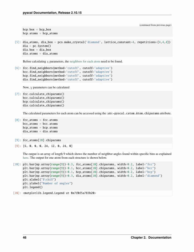
[9]: fcc_atoms[10].chiparams

[9]: [6, 0, 0, 0, 24, 12, 0, 24, 0]

The output is an array of length 9 which shows the number of neighbor angles found within specific bins as explainedhere. The output for one atom from each structure is shown below.

[10]: plt.bar(np.array(range(9))-0.3, fcc_atoms[10].chiparams, width=0.2, label="fcc")plt.bar(np.array(range(9))-0.1, bcc_atoms[10].chiparams, width=0.2, label="bcc")plt.bar(np.array(range(9))+0.1, hcp_atoms[10].chiparams, width=0.2, label="hcp")plt.bar(np.array(range(9))+0.3, dia_atoms[10].chiparams, width=0.2, label="diamond")plt.xlabel("$\chi$")plt.ylabel("Number of angles")plt.legend()

[10]: <matplotlib.legend.Legend at 0x7f0f5a783b20>

46 Chapter 2. Documentation

pyscal Documentation, Release 2.10.15

The atoms exhibit a distinct fingerprint for each structure. Structural identification can be made up comparing the ratioof various 𝜒 parameters as described in the original publication.

Centrosymmetry parameter

Centrosymmetry parameter (CSP) was introduced by *Kelchner et al.* to identify defects in crystals. The parametermeasures the loss of local symmetry. For an atom with 𝑁 nearest neighbors, the parameter is given by,

CSP =

𝑁/2∑𝑖=1

r𝑖 + r𝑖+𝑁/2

2r𝑖 and r𝑖+𝑁/2 are vectors from the central atom to two opposite pairs of neighbors. There are two main methods toidentify the opposite pairs of neighbors as described in this publication. Pyscal uses the first approach called *GreedyEdge Selection*(GES) and is implemented in LAMMPS and Ovito. GES algorithm calculates a weight 𝑤𝑖𝑗 = |r𝑖 +r𝑗 |for all combinations of neighbors around an atom and calculates CSP over the smallest 𝑁/2 weights.

A centrosymmetry parameter calculation using GES algorithm can be carried out as follows. First we can try a perfectcrystal.

[4]: import pyscal as pcimport pyscal.crystal_structures as pcs

import matplotlib.pyplot as plt

[5]: atoms, box = pcs.make_crystal(structure='fcc', lattice_constant=4.0, repetitions=(3,3,3))

[6]: sys = pc.System()sys.box = boxsys.atoms = atomscsm = sys.calculate_centrosymmetry(nmax = 12)

[8]: plt.plot(csm, 'o')

[8]: [<matplotlib.lines.Line2D at 0x7fdb95d78370>]

2.3. Methods and examples 47

pyscal Documentation, Release 2.10.15

You can see all values are zero, as expected. Now lets add some noise to the structure and see how the centrosymmetryparameter changes.

[9]: atoms, box = pcs.make_crystal(structure='fcc', lattice_constant=4.0, repetitions=(3,3,3),→˓ noise=0.1)

[10]: sys = pc.System()sys.box = boxsys.atoms = atomscsm = sys.calculate_centrosymmetry(nmax = 12)

[11]: plt.plot(csm, 'o')

[11]: [<matplotlib.lines.Line2D at 0x7fdb95cfc9d0>]

The centrosymmetry parameter shows a distribution, owing to the thermal vibrations.

nmax parameter specifies the number of nearest neighbors to be considered for the calculation of CSP. If bcc structureis used, this should be changed to either 8 or 14.

48 Chapter 2. Documentation

pyscal Documentation, Release 2.10.15

Cowley short range order parameter

The Cowley short range order parameter can be used to find if an alloy is ordered or not. The order parameter is givenby,

𝛼𝑖 = 1 − 𝑛𝑖

𝑚𝐴𝑐𝑖

where 𝑛𝑖 is the number of atoms of the non reference type among the 𝑐𝑖 atoms in the 𝑖th shell. 𝑚𝐴 is the concentrationof the non reference atom.

We can start by importing the necessary modules

[1]: import pyscal as pcimport pyscal.crystal_structures as pcsimport matplotlib.pyplot as plt

We need a binary alloy structure to calculate the order parameter. We will use the crystal structures modules to do this.Here, we will create a L12 structure.

[2]: atoms, box = pcs.make_crystal('l12', lattice_constant=4.00, repetitions=[2,2,2])

In order to use the order parameter, we need to have two shells of neighbors around the atom. In order to get two shellsof neighbors, we will first estimate a cutoff using the radial distribution function.

[4]: sys = pc.System()sys.box = boxsys.atoms = atoms

[5]: val, dist = sys.calculate_rdf()

We can plot the rdf,

[7]: plt.plot(dist, val)plt.xlabel(r"distance $\AA$")plt.ylabel(r"$g(r)$")plt.xlim(0, 5)

[7]: (0.0, 5.0)

2.3. Methods and examples 49

pyscal Documentation, Release 2.10.15

In this case, a cutoff of about 4.5 will make sure that two shells are included. Now the neighbors are calculated usingthis cutoff.

[8]: sys.find_neighbors(method='cutoff', cutoff=4.5)

Finally we can calculate the short range order. We will use the reference type as 1 and also specify the average keywordas True. This will allow us to get an average value for the whole simulation box.

[9]: sys.calculate_sro(reference_type=1, average=True)

[9]: array([-0.33333333, 1. ])

Value for individual atoms can be accessed by,

[10]: atoms = sys.atoms

[11]: atoms[4].sro

[11]: [-0.33333333333333326, 1.0]

Only atoms of the non reference type will have this value!

Entropy parameters

In this example, the entropy parameters are calculated and used for distinction of solid and liquid. For a description ofentropy parameters, see here.

[1]: import pyscal.core as pcimport matplotlib.pyplot as pltimport numpy as np

We have two test configurations for Al at 900 K, one is fcc structured and the other one is in liquid state. We calculatethe entropy parameters for each of these configurations. First we start by reading in the fcc configuration. For entropyparameters, the values of the integration limit 𝑟𝑚 is chosen as 1.4, based on the original publication.

[2]: sys = pc.System()sys.read_inputfile("../tests/conf.fcc.Al.dump")sys.find_neighbors(method="cutoff", cutoff=0)

The values of 𝑟𝑚 is in units of lattice constant, so we need to calculate the lattice constant first. Since is a cubic box,we can do this by,

[3]: lat = (sys.box[0][1]-sys.box[0][0])/5

Now we calculate the entropy parameter and its averaged version. Averaging can be done in two methods, as a sim-ple average over neighbors or using a switching function. We will use a simple averaging over the neighbors. Thelocal keyword allows to use a local density instead of the global one. However, this only works if the neighbors werecalculated using a cutoff method.

[4]: sys.calculate_entropy(1.4*lat, averaged=True, local=True)

The calculated values are stored for each atom. This can be accessed as follows,

[5]: atoms = sys.atomssolid_entropy = [atom.entropy for atom in atoms]solid_avg_entropy = [atom.avg_entropy for atom in atoms]

50 Chapter 2. Documentation

pyscal Documentation, Release 2.10.15

Now we can quickly repeat the calculation for the liquid structure.

[6]: sys = pc.System()sys.read_inputfile("../tests/conf.lqd.Al.dump")sys.find_neighbors(method="cutoff", cutoff=0)lat = (sys.box[0][1]-sys.box[0][0])/5sys.calculate_entropy(1.4*lat, local=True, averaged=True)atoms = sys.atomsliquid_entropy = [atom.entropy for atom in atoms]liquid_avg_entropy = [atom.avg_entropy for atom in atoms]

Finally we can plot the results

[7]: xmin = -3.55xmax = -2.9bins = np.arange(xmin, xmax, 0.01)x = plt.hist(solid_entropy, bins=bins, density=True, alpha=0.5, color="#EF9A9A")x = plt.hist(solid_avg_entropy, bins=bins, density=True, alpha=0.5, color="#B71C1C")x = plt.hist(liquid_entropy, bins=bins, density=True, alpha=0.5, color="#90CAF9")x = plt.hist(liquid_avg_entropy, bins=bins, density=True, alpha=0.5, color="#0D47A1")plt.xlabel(r"$s_s^i$")

[7]: Text(0.5, 0, '$s_s^i$')

The distributions of 𝑠𝑖𝑠 given in light red and light blue are fairly distinct but show some overlap. The averaged entropyparameter, 𝑠𝑖𝑠 show distinct peaks which can distinguish solid and liquid very well.

[8]: np.mean(solid_entropy), np.mean(solid_avg_entropy)

[8]: (-3.47074287018929, -3.47074287018929)

2.3. Methods and examples 51

pyscal Documentation, Release 2.10.15

Calculating energy

pyscal can also be used for quick energy calculations. The energy per atom can give an insight into the local environ-ment. pyscal relies on the python library interface of LAMMPS for calculation of energy. The python library interface,hence, is a requirement for energy calculation. The easiest way to set up the LAMMPS library is by installing LAMMPSthrough the conda package.

conda install -c conda-forge lammps

Alternatively, this page provides information on how to compile manually.

Interatomic potentials

An interatomic potential is also required for the calculation of energy. The potential can be of any type that LAMMPSsupports. For this example, we will use an EAM potential for Mo which is provided in the file Mo.set.

We start by importing the necessary modules,

[1]: import pyscal.core as pcimport matplotlib.pyplot as pltimport numpy as np

For this example, a LAMMPS dump file will be read in and the energy will be calculated.

[2]: sys = pc.System()sys.read_inputfile("conf.bcc.dump")

Now the energy can be calculated by,

[3]: sys.calculate_energy(species=['Mo'], pair_style='eam/alloy',pair_coeff='* * Mo.set Mo', mass=95)

The first keyword above is species, which specifies the atomic species. This is required for ASE module whichis used under the hood for convertion of files. pair_style species the type of potential used in LAMMPS. Seedocumentation here. pair_coeff is another LAMMPS command which is documented well here. Also, the massneeds to be provided.

Once the calculation is over, the energy can be accessed for each atom as follows,

[4]: atoms = sys.atoms

[5]: atoms[0].energy

[5]: -6.743130736133679

It is also possible to find the energy averaged over the neighbors using the averaged keyword. However, a neighborcalculation should be done before.

[6]: sys.find_neighbors(method="cutoff", cutoff=0)sys.calculate_energy(species=['Mo'], pair_style='eam/alloy',

pair_coeff='* * Mo.set Mo', mass=95, averaged=True)

[7]: atoms = sys.atomsatoms[0].avg_energy

52 Chapter 2. Documentation

pyscal Documentation, Release 2.10.15

[7]: -6.534395941639571

We have two test configurations for Al at 900 K, one is fcc structured and the other one is in liquid state. We calculatethe energy parameters for each of these configurations.

[8]: sys = pc.System()sys.read_inputfile("../tests/conf.fcc.Al.dump")sys.find_neighbors(method="cutoff", cutoff=0)

[9]: sys.calculate_energy(species=['Al'], pair_style='eam/alloy',pair_coeff='* * Al.eam.fs Al', mass=26.98, averaged=True)

Now lets gather the energies

[10]: atoms = sys.atomssolid_energy = [atom.energy for atom in atoms]solid_avg_energy = [atom.avg_energy for atom in atoms]

We can repeat the calculations for the liquid phase,

[11]: sys = pc.System()sys.read_inputfile("../tests/conf.lqd.Al.dump")sys.find_neighbors(method="cutoff", cutoff=0)sys.calculate_energy(species=['Al'], pair_style='eam/alloy',

pair_coeff='* * Al.eam.fs Al', mass=26.98, averaged=True)atoms = sys.atomsliquid_energy = [atom.energy for atom in atoms]liquid_avg_energy = [atom.avg_energy for atom in atoms]

Finally we can plot the results

[13]: xmin = -3.5xmax = -2.5bins = np.arange(xmin, xmax, 0.01)x = plt.hist(solid_energy, bins=bins, density=True, alpha=0.5, color="#EF9A9A")x = plt.hist(solid_avg_energy, bins=bins, density=True, alpha=0.5, color="#B71C1C")x = plt.hist(liquid_energy, bins=bins, density=True, alpha=0.5, color="#90CAF9")x = plt.hist(liquid_avg_energy, bins=bins, density=True, alpha=0.5, color="#0D47A1")plt.xlabel(r"Energy")

[13]: Text(0.5, 0, 'Energy')

2.3. Methods and examples 53

pyscal Documentation, Release 2.10.15

Entropy and enthalpy parameters

In this example, energy and entropy parameters will be used for structural distinction. We will consider bcc, fcc, andhcp structures to calculate the parameters.

[1]: import pyscal.core as pcimport pyscal.crystal_structures as pcsimport numpy as npimport matplotlib.pyplot as plt

Now we will create some structures with thermal vibrations

[2]: bcc_atoms, bcc_box = pcs.make_crystal('bcc',lattice_constant=3.147,repetitions=[10,10,10], noise=0.1)

bcc = pc.System()bcc.atoms = bcc_atomsbcc.box = bcc_box

[3]: fcc_atoms, fcc_box = pcs.make_crystal('fcc',lattice_constant=3.147,repetitions=[10,10,10], noise=0.1)

fcc = pc.System()fcc.atoms = fcc_atomsfcc.box = fcc_box

[4]: hcp_atoms, hcp_box = pcs.make_crystal('hcp',lattice_constant=3.147,repetitions=[10,10,10], noise=0.1)

hcp = pc.System()hcp.atoms = hcp_atomshcp.box = hcp_box

The next step is to calculate the neighbors using adaptive cutoff

54 Chapter 2. Documentation

pyscal Documentation, Release 2.10.15

[5]: bcc.find_neighbors(method='cutoff', cutoff=0)fcc.find_neighbors(method='cutoff', cutoff=0)hcp.find_neighbors(method='cutoff', cutoff=0)

In order to calculate energy, a molybdenum potential is used here.

[6]: bcc.calculate_energy(species=['Mo'], pair_style='eam/alloy',pair_coeff='* * Mo.set Mo', mass=95,averaged=True)

fcc.calculate_energy(species=['Mo'], pair_style='eam/alloy',pair_coeff='* * Mo.set Mo', mass=95,averaged=True)

hcp.calculate_energy(species=['Mo'], pair_style='eam/alloy',pair_coeff='* * Mo.set Mo', mass=95,averaged=True)

Now we will calculate the entropy parameters

[7]: latbcc = (bcc.box[0][1]-bcc.box[0][0])/10latfcc = (fcc.box[0][1]-fcc.box[0][0])/10lathcp = (hcp.box[0][1]-hcp.box[0][0])/10

[8]: bcc.calculate_entropy(1.4*latbcc, averaged=True, local=True)fcc.calculate_entropy(1.4*latfcc, averaged=True, local=True)hcp.calculate_entropy(1.4*lathcp, averaged=True, local=True)

Gather the values

[9]: bccenergy = [atom.energy for atom in bcc.atoms]avgbccenergy = [atom.avg_energy for atom in bcc.atoms]fccenergy = [atom.energy for atom in fcc.atoms]avgfccenergy = [atom.avg_energy for atom in fcc.atoms]hcpenergy = [atom.energy for atom in hcp.atoms]avghcpenergy = [atom.avg_energy for atom in hcp.atoms]

[10]: bccentropy = [atom.entropy for atom in bcc.atoms]avgbccentropy = [atom.avg_entropy for atom in bcc.atoms]fccentropy = [atom.entropy for atom in fcc.atoms]avgfccentropy = [atom.avg_entropy for atom in fcc.atoms]hcpentropy = [atom.entropy for atom in hcp.atoms]avghcpentropy = [atom.avg_entropy for atom in hcp.atoms]

[13]: plt.scatter(fccenergy, fccentropy, s=10, label='fcc', color='#FFB300')plt.scatter(hcpenergy, hcpentropy, s=10, label='hcp', color='#388E3C')plt.scatter(bccenergy, bccentropy, s=10, label='bcc', color='#C62828')plt.xlabel("Energy")plt.ylabel("Entropy")plt.legend()

[13]: <matplotlib.legend.Legend at 0x7f82fd6bc690>

2.3. Methods and examples 55

pyscal Documentation, Release 2.10.15

[14]: plt.scatter(avgfccenergy, avgfccentropy, s=10, label='fcc', color='#FFB300')plt.scatter(avghcpenergy, avghcpentropy, s=10, label='hcp', color='#388E3C')plt.scatter(avgbccenergy, avgbccentropy, s=10, label='bcc', color='#C62828')plt.xlabel("Avg Energy")plt.ylabel("Avg Entropy")plt.legend()

[14]: <matplotlib.legend.Legend at 0x7f82fd615d90>

56 Chapter 2. Documentation

pyscal Documentation, Release 2.10.15

Visualizing System objects

In this notebook, experimental plotting methods of pyscal is illustrated. The plotting functionality works only throughjupyter notebooks or jupyter lab. It depends on ipywidgets and plotly to render the output. There is some extra config-uration that needs to be done which can be found here.

In short, for jupyter lab (>3):

pip install "jupyterlab>=3" "ipywidgets>=7.6"pip install jupyter-dash

In notebooks:

pip install "notebook>=5.3" "ipywidgets>=7.5"

We start by importing the necessary modules

[1]: import pyscal as pc

Now we can set up a system and read in a file to be visualized

[2]: sys = pc.System()sys.read_inputfile("conf8k.dump", customkeys=["vx", "vy", "vz"])

We will further calculate some q values and also the solid particles in the system which will be used later for visualization

[3]: sys.find_neighbors(method="cutoff", cutoff=0)sys.calculate_q([4, 5, 6], averaged=True)sys.find_solids()

[3]: 448

In order to visualize the system, the show method can be used. This method renders a widget which a slider for theradius of atoms and a text box for entering the colormap to be used for coloring atoms. A list of colormaps can befound here. The widget also has a Render plot button which will generate the plot.

[4]: sys.show()

interactive(children=(FloatSlider(value=1.0, description='radius', max=30.0, min=1.0,␣→˓step=1.0), Text(value='S...

This is just a general rendering of the system. Further customization can be done. For example, we can color the atomsusing the averaged q6 values.

[5]: sys.show(colorby="aq6")

interactive(children=(FloatSlider(value=1.0, description='radius', max=30.0, min=1.0,␣→˓step=1.0), Text(value='S...

We can also select which atoms are to be plotted. For example we can refine the figure to only plot the atoms that areidentified as solid in the find_solids method.

[6]: sys.show(colorby="aq6", filterby="solid")

interactive(children=(FloatSlider(value=1.0, description='radius', max=30.0, min=1.0,␣→˓step=1.0), Text(value='S...

2.3. Methods and examples 57

pyscal Documentation, Release 2.10.15

Any atom property can used to color the map. These include any Atom attribute, calculated q values which can beaccessed by qx or aqx, for traditional and averaged Steinhardts parameters respectively. x stands for the number of q.It can also be attributes that are stored in the Atom.custom variable. In the above code bit, when the file was read in, thecustom variable was used to read in the velocities for each atom. We will color atoms using the velocity in x direction,that is vx attribute.

[7]: sys.show(colorby="vx")

interactive(children=(FloatSlider(value=1.0, description='radius', max=30.0, min=1.0,␣→˓step=1.0), Text(value='S...

pyscal Trajectory

Trajectory is a pyscal module intended for working with molecular dynamics trajectories which contain more thanone time slice. Currently, the module only supports LAMMPS dump text file formats. It can be used to get a single orslices from a trajectory, trim the trajectory or even combine multiple trajectories. The example below illustrates varioususes of the module.

``Trajectory`` is an experimental feature at the moment and may undergo significant changes in future releasesStart with importing the module

[1]: from pyscal import Trajectory

Read in a trajectory.

[2]: traj = Trajectory("traj.light")

When using the above statement, the trajectory is not yet read in to memory. Just the basic information is availablenow.

[3]: traj

[3]: Trajectory of 10 slices with 500 atoms

We can know the number of slices in the trajectory and the number of atoms. Trajectory only works with fixednumber of atoms.

Now, one can get a single slice or multiple slices just as is done with a python list. Getting the 2nd slice (counting startsfrom 0!).

[4]: sl = traj[2]sl

[4]: Trajectory slice2-2natoms=500

This slice can now be converted to a more usable format, either to a pyscal System or just written to another text file.Convert to a pyscal System object,

[5]: sys = sl.to_system()sys

[5]: [<pyscal.core.System at 0x7f81f93971d0>]

System objects contain all the information. The atomic positions, simulation box and so on are easily accessible.

58 Chapter 2. Documentation

pyscal Documentation, Release 2.10.15

[6]: sys[0].box

[6]: [[18.22887, 0.0, 0.0], [0.0, 18.234740000000002, 0.0], [0.0, 0.0, 18.37877]]

[7]: sys[0].atoms[0].pos

[7]: [-4.9941, -6.34185, -6.8551]

If information other than positions are required, the customkeys keyword can be used. For example, for velocity inthe x direction,

[8]: sys = sl.to_system(customkeys=["vx"])sys

[8]: [<pyscal.core.System at 0x7f81f9397530>]

[9]: sys[0].atoms[0].custom["vx"]

[9]: '-1.21558'

Instead of creating a System object, the slice can also be written to a file directly.

[10]: sl.to_file("test.dump")

Like normal python lists, multiple slices can also be accessed directly

[12]: sl1 = traj[0:4]sl1

[12]: Trajectory slice0-3natoms=500

to_system and to_file methods can be used on this object too.

Multiple slices can be added together

[13]: sl2 = traj[5:7]sl2

[13]: Trajectory slice5-6natoms=500

[14]: slnew = sl1+sl2slnew

[14]: Trajectory slice0-3/5-6natoms=500

Once again, one could write the combined trajectory slice to a file, or create a System object out of it.

2.3. Methods and examples 59

pyscal Documentation, Release 2.10.15

2.4 pyscal reference

2.4.1 pyscal Reference

pyscal.core module

Main module of pyscal. This module contains definitions of the two major classes in pyscal - the System and Atom .Atom is a pure pybind11 class whereas System is a hybrid class with additional python definitions. For the ease of use,Atom class should be imported from the core module. The original pybind11 definitions of Atom and System can befound in catom and csystem respectively.

class pyscal.core.SystemBases: pyscal.csystem.System

A python/pybind11 hybrid class for holding the properties of a system.

boxA list containing the dimensions of the simulation box in the format [[x_low, x_high], [y_low, y_high],[z_low, z_high]]

Type list of list of floats

atoms

Type list of Atom objects

Notes

A System consists of two major components - the simulation box and the atoms. All the associated variables arethen calculated using this class.

Note: atoms can be accessed or set as atoms. However, due to technical reasons individual atoms should beaccessed using the get_atom() method. An atom can be assigned to the atom using the set_atom() method.

Examples

>>> sys = System()>>> sys.read_inputfile('atoms.dat')

__init__()

add_atoms(atoms)Add a given list of atoms

Parameters atoms (List of Atoms) –

ReturnsReturn type None

property atomsAtom access

property boxWrap for inbuilt box

60 Chapter 2. Documentation

pyscal Documentation, Release 2.10.15

calculate_angularcriteria()Calculate the angular criteria for each atom :param None:

ReturnsReturn type None

Notes

Calculates the angular criteria for each atom as defined in [1]_. Angular criteria is useful for identificationof diamond cubic structures. Angular criteria is defined by,

𝐴 =

6∑𝑖=1

(cos(𝜃𝑖) +1

3)2

where cos(theta) is the angle size suspended by each pair of neighbors of the central atom. A will have avalue close to 0 for structures if the angles are close to 109 degrees. The calculated A parameter for eachatom is stored in angular.

References

calculate_centrosymmetry(nmax=12, get_vals=True)Calculate the centrosymmetry parameter

Parameters nmax (int, optional) – number of neighbors to be considered for centrosymme-try parameters. Has to be a positive, even integer. Default 12

ReturnsReturn type None

Notes

Calculate the centrosymmetry parameter for each atom which can be accessed by centrosymmetry at-tribute. It calculates the degree of inversion symmetry of an atomic environment. Centrosymmetry recalcu-lates the neighbor using the number method as specified in ¬pyscal.core.System.find_neighbors()method. This is the ensure that the required number of neighbors are found for calculation of the parameter.

The Greedy Edge Selection (GES) [1] as specified in [2] in used in this method. GES algorithm is imple-mented in LAMMPS and Ovito. Please see [2] for a detailed description of the algorithms.

References

calculate_chiparams(angles=False)Calculate the chi param vector for each atom

Parameters angles (bool, optional) – If True, return the list of cosines of all neighbor pairs

Returns angles – list of all cosine values, returned only if angles is True.

Return type array of floats

2.4. pyscal reference 61

pyscal Documentation, Release 2.10.15

Notes

This method tries to distinguish between crystal structures by finding the cosines of angles formed by anatom with its neighbors. These cosines are then historgrammed with bins [-1.0, -0.945, -0.915, -0.755,-0.705, -0.195, 0.195, 0.245, 0.795, 1.0] to find a vector for each atom that is indicative of its local coor-dination. Compared to chi parameters from chi_0 to chi_7 in the associated publication, the vector here isfrom chi_0 to chi_8. This is due to an additional chi parameter which measures the number of neighborsbetween cosines -0.705 to -0.195.

Parameter nlimit specifies the number of nearest neighbors to be included in the analysis to find the cutoff.If parameter angles is true, an array of all cosine values is returned. The publication further providescombinations of chi parameters for structural identification which is not implemented here. The calculatedchi params can be accessed using chiparams.

References

calculate_cna(lattice_constant=None)Calculate the Common Neighbor Analysis indices

Parameters lattice_constant (float, optional) – lattice constant to calculate CNA. Ifnot specified, adaptive CNA will be used

Returns cna – dict containing the cna signature of the system

Return type dict

Notes

Performs the common neighbor analysis [1][2] or the adaptive common neighbor analysis [2] and assignsa structure to each atom.

If lattice_constant is specified, a convential common neighbor analysis is used. If lattice_constant isnot specified, adaptive common neighbor analysis is used. The assigned structures can be accessed bystructure. The values assigned for stucture are 0 Unknown, 1 fcc, 2 hcp, 3 bcc, 4 icosahedral.

References

calculate_disorder(averaged=False, q=6)Calculate the disorder criteria for each atom

Parameters• averaged (bool, optional) – If True, calculate the averaged disorder. Default False.

• q (int, optional) – The Steinhardt parameter value over which the bonds have to becalculated. Default 6.

ReturnsReturn type None

62 Chapter 2. Documentation

pyscal Documentation, Release 2.10.15

Notes

Calculate the disorder criteria as introduced in [1]. The disorder criteria value for each atom is defined by,

𝐷𝑗 =1

𝑁 𝑗𝑏

𝑁𝑏∑𝑖=1

[𝑆𝑗𝑗 + 𝑆𝑘𝑘 − 2𝑆𝑗𝑘]

where .. math:: S_{ij} = sum_{m=-6}^6 q_{6m}(i) q_{6m}^*(i)

The keyword averaged is True, the disorder value is averaged over the atom and its neighbors. The disordervalue can be accessed using disorder and the averaged version can be accessed using avg_disorder.For ordered systems, the value of disorder would be zero which would increase and reach one for disorderedsystems.

References

calculate_energy(species='Au', pair_style=None, pair_coeff=None, mass=1.0, averaged=False)Calculate the potential energy of atom using LAMMPS

Parameters• species (str) – Name of atomic species

• pair_style (str) – lammps pair style

• pair_coeff (str) – lammps pair coeff

• mass (float) – mass of the atoms

• averaged (bool, optional) – Average the energy over neighbors if True default False.

ReturnsReturn type None

Notes

Calculates the potential energy per atom using the given potential through LAMMPS. More documentationcoming up. . .

Values can be accessed through pyscal.catom.Atom.energy Averaged values can be accessed throughpyscal.catom.Atom.avg_energy

If averaged is True, the energy is averaged over the neighbors of an atom. If neighbors were calculatedbefore calling this method, those neighbors are used for averaging. Otherwise neighbors are calculated onthe fly with an adaptive cutoff method.

calculate_entropy(rm, sigma=0.2, rstart=0.001, h=0.001, local=False, M=12, N=6, ra=None,averaged=False, switching_function=False)

Calculate the entropy parameter for each atom

Parameters• rm (float) – cutoff distance for integration of entropy parameter in distance units

• sigma (float) – broadening parameter

• rstart (float, optional) – minimum limit for integration, default 0.00001

• h (float, optional) – width for trapezoidal integration, default 0.0001

2.4. pyscal reference 63

pyscal Documentation, Release 2.10.15

• local (bool, optional) – if True, use the local density instead of global density defaultFalse

• averaged (bool, optional) – if True find the averaged entropy parameters default False

• switching_function (bool, optional) – if True, use the switching function to aver-age, otherwise do a simple average over the neighbors. Default False

• ra (float, optional) – cutoff length for switching function used only if switch-ing_function is True

• M (int, optional) – power for switching function, default 12 used only if switch-ing_function is True

• N (int, optional) – power for switching function, default 6 used only if switch-ing_function is True

ReturnsReturn type None

Notes

The entropy parameters can be accessed by entropy and avg_entropy. For a complete description of theentropy parameter, see the documentation

The local keyword can be used to use a local density instead of the global one. This method will only workwith neighbor methods that use a cutoff.

calculate_pmsro(reference_type=1, compare_type=2, average=True, shells=2, delta=True)Calculate pairwise multicomponent short range order

Parameters• reference_type (int, optional) – type of the atom to be used a reference. default 1

• compare_type (int, optional) – type of the atom to be used to compare. default 2

• average (bool, optional) – if True, average over all atoms of the reference type in thesystem. default True.

• delta (bool, optional) – if True, SRO calculation contain the Kronecker delta in thedefinition. if False, delta is always 0, and the function return the Cowley-SRO value. defaultTrue.

Returns vec – The short range order averaged over the whole system for atom of the referencetype. Only returned if average is True. First value is SRO of the first neighbor shell and thesecond value corresponds to the second nearest neighbor shell.

Return type list of float

64 Chapter 2. Documentation

pyscal Documentation, Release 2.10.15

Notes

Calculates the pairwise multicomponent short range order for a higher-dimensional systems alloy using theapproach by Fontaine [1]. Pairwise multicomponent short range order is calculated as,

𝛼𝑖𝑗 =𝑛𝑗/𝑚𝐴− 𝑐𝑗

𝛿𝑖𝑗 − 𝑐𝑗

where i refers to reference type. n_j is the number of atoms of the non reference type among the c_j atomsin the ith shell. m_A is the concentration of the non reference atom. delta_{ij}” = 1 if i = j. Please notethat the value is calculated for shells 1 and 2 by default. In order for this to be possible, neighbors haveto be found first using the find_neighbors() method. The selected neighbor method should include thesecond shell as well. For this purpose method=cutoff can be chosen with a cutoff long enough to includethe second shell. In order to estimate this cutoff, one can use the calculate_rdf() method.

References

calculate_q(q, averaged=False, only_averaged=False, condition=None, clear_condition=False)Find the Steinhardt parameter q_l for all atoms.

Parameters• q_l (int or list of ints) – A list of all Steinhardt parameters to be found from 2-12.

• averaged (bool, optional) – If True, return the averaged q values, default False

• only_averaged (bool, optional) – If True, only calculate the averaged part. defaultFalse

• condition (callable or atom property) – Either function which should take anAtom object, and give a True/False output or an attribute of atom class which has valueor 1 or 0.

• clear_condition (bool, optional) – clear the condition variable for all atoms

ReturnsReturn type None

Notes

Enables calculation of the Steinhardt parameters [1] q from 2-12. The type of q values depend on themethod used to calculate neighbors. See the description find_neighbors() for more details. If thekeyword average is set to True, the averaged versions of the bond order parameter [2] is returned. If onlythe averaged versions need to be calculated, only_averaged keyword can be set to False.

The neighbors over which the q values are calculated can also be filtered. This is done through the argu-ment condition which is passed as a parameter. condition can be of two types. The first type is a functionwhich takes an Atom object and should give a True/False value. condition can also be an Atom attribute ora value from custom values stored in an atom. See cluster_atoms() for more details. If the conditionis equal for both host atom and the neighbor, the neighbor is considered for calculation of q parameters.This is slightly different from cluster_atoms() where the condition has to be True for both atoms. con-dition is only cleared when neighbors are recalculated. Additionally, the keyword clear_condition can alsobe used to clear the condition and reset it to 0. By default, condition is applied to both unaveraged andaveraged q parameter calculation. If condition is needed for only averaged q parameters, this function canbe called twice, initially without condition and averaged=False, and then with a condition specified andaveraged=True. This way, the condition will only be applied to the averaged q calculation.

2.4. pyscal reference 65

pyscal Documentation, Release 2.10.15

References

calculate_rdf(histobins=100, histomin=0.0, histomax=None)Calculate the radial distribution function.

Parameters• histobins (int) – number of bins in the histogram

• histomin (float, optional) – minimum value of the distance histogram. Default 0.0.

• histomax (float, optional) – maximum value of the distance histogram. Default, themaximum value in all pair distances is used.

Returns• rdf (array of ints) – Radial distribution function

• r (array of floats) – radius in distance units

calculate_solidneighbors()Find Solid neighbors of all atoms in the system.

Parameters None –

ReturnsReturn type None

Notes

A solid bond is considered between two atoms if the connection between them is greater than 0.6.

calculate_sro(reference_type=1, average=True, shells=2)Calculate short range order

Parameters• reference_type (int, optional) – type of the atom to be used a reference. default 1

• average (bool, optional) – if True, average over all atoms of the reference type in thesystem. default True.

Returns vec – The short range order averaged over the whole system for atom of the referencetype. Only returned if average is True. First value is SRO of the first neighbor shell and thesecond value corresponds to the second nearest neighbor shell.

Return type list of float

Notes

Calculates the short range order for an AB alloy using the approach by Cowley [1]. Short range order iscalculated as,

𝛼𝑖 = 1 − 𝑛𝑖

𝑚𝐴𝑐𝑖

where n_i is the number of atoms of the non reference type among the c_i atoms in the ith shell. m_A is theconcentration of the non reference atom. Please note that the value is calculated for shells 1 and 2 by default.In order for this to be possible, neighbors have to be found first using the find_neighbors()method. Theselected neighbor method should include the second shell as well. For this purpose method=cutoff can bechosen with a cutoff long enough to include the second shell. In order to estimate this cutoff, one can usethe calculate_rdf() method.

66 Chapter 2. Documentation

pyscal Documentation, Release 2.10.15

References

calculate_vorovector(edge_cutoff=0.05, area_cutoff=0.01, edge_length=False)get the voronoi structure identification vector.

Parameters edge_cutoff (float, optional) – cutoff for edge length. Default 0.05.

area_cutoff [float, optional] cutoff for face area. Default 0.01.

edge_length [bool, optional] if True, a list of unrefined edge lengths are returned. Default false.

Returns vorovector – array of the form (n3, n4, n5, n6)

Return type array like, int

Notes

Returns a vector of the form (n3, n4, n5, n6), where n3 is the number of faces with 3 vertices, n4 is thenumber of faces with 4 vertices and so on. This can be used to identify structures [1] [2].

The keywords edge_cutoff and area_cutoff can be used to tune the values to minimise the effect of ther-mal distortions. Edges are only considered in the analysis if the edge_length/sum(edge_lengths) is at leastedge_cutoff. Similarly, faces are only considered in the analysis if the face_area/sum(face_areas) is at leastface_cutoff.

References

cluster_atoms(condition, largest=True, cutoff=0)Cluster atoms based on a property

Parameters• condition (callable or atom property) – Either function which should take anAtom object, and give a True/False output or an attribute of atom class which has valueor 1 or 0.

• largest (bool, optional) – If True returns the size of the largest cluster. Default False.

• cutoff (float, optional) – If specified, use this cutoff for calculation of clusters. Bydefault uses the cutoff used for neighbor calculation.

Returns lc – Size of the largest cluster. Returned only if largest is True.

Return type int

Notes

This function helps to cluster atoms based on a defined property. This property is defined by the userthrough the argument condition which is passed as a parameter. condition can be of two types. The firsttype is a function which takes an Atom object and should give a True/False value. condition can also be anAtom attribute or a value from custom values stored in an atom.

When clustering, the code loops over each atom and its neighbors. If the condition is true for both hostatom and the neighbor, they are assigned to the same cluster. For example, a condition to cluster solid atomswould be,

2.4. pyscal reference 67

pyscal Documentation, Release 2.10.15

def condition(atom):#if both atom is solidreturn (atom1.solid)

The same can be done by passing “solid” as the condition argument instead of the above function. Passinga function allows to evaluate complex conditions, but is slower than passing an attribute.

embed_in_cubic_box()Embedded the triclinic box in a cubic box

extract_cubic_box(repeat=(3, 3, 3))Extract a cubic representation of the box from triclinic cell

Parameters repeat (list of ints) – the number of times box should be repeat

Returns• cubebox (list of list of floats) – cubic box

• atoms (list of Atom objects) – atoms in the cubic box

find_diamond_neighbors()Find underlying fcc lattice in diamond

Parameters None –

ReturnsReturn type None

Notes

This method finds in the underlying fcc/hcp lattice in diamond. It works by the method described in thispublication . For each atom, 4 atoms closest to it are identified. The neighbors of the its neighbors arefurther identified and the common neighbors shared with the host atom are selected. These atom will fallin the underlying fcc lattice for cubic diamond or hcp lattice for hexagonal lattice.

If neighbors are previously calculated, they are reset when this method is used.

find_largestcluster()Find the largest solid cluster of atoms in the system from all the clusters.

Parameters None –

Returns cluster – the size of the largest cluster

Return type int

Notes

pyscal.core.System.find_clusters() has to be used before using this function.

find_neighbors(method='cutoff', cutoff=None, threshold=2, filter=None, voroexp=1, padding=1.2,nlimit=6, cells=False, nmax=12, assign_neighbor=True)

Find neighbors of all atoms in the System .

Parameters method ({'cutoff', 'voronoi', 'number'}) – cutoff method finds neighbors ofan atom within a specified or adaptive cutoff distance from the atom. voronoi method findsatoms that share a Voronoi polyhedra face with the atom. Default, cutoff number methodfinds a specified number of closest neighbors to the given atom. Number only populates

68 Chapter 2. Documentation

pyscal Documentation, Release 2.10.15

cutoff [{ float, ‘sann’, ‘adaptive’}] the cutoff distance to be used for the cutoff based neighbor calculationmethod described above. If the value is specified as 0 or adaptive, adaptive method is used. If thevalue is specified as sann, sann algorithm is used.

threshold [float, optional] only used if cutoff=adaptive. A threshold which is used as safe limit forcalculation of cutoff.

filter [{‘None’, ‘type’, ‘type_r’}, optional] apply a filter to nearest neighbor calculation. If the filter key-word is set to type, only atoms of the same type would be included in the neighbor calculations. Iftype_r, only atoms of a different type will be included in the calculation. Default None.

voroexp [int, optional] only used if method=voronoi. Power of the neighbor weight used to weight thecontribution of each atom towards Steinhardt parameter values. Default 1.

padding [double, optional] only used if cutoff=adaptive or cutoff=number. A safe padding valueused after an adaptive cutoff is found. Default 1.2.

nlimit [int, optional] only used if cutoff=adaptive. The number of particles to be considered for thecalculation of adaptive cutoff. Default 6.

nmax [int, optional] only used if cutoff=number. The number of closest neighbors to be found for eachatom. Default 12

ReturnsReturn type None

Raises• RuntimeWarning – raised when threshold value is too low. A low threshold value will

lead to ‘sann’ algorithm not converging when finding a neighbor. This function will try toautomatically increase threshold and check again.

• RuntimeError – raised when neighbor search was unsuccessful. This is due to a lowthreshold value.

Notes

This function calculates the neighbors of each particle. There are several ways to do this. A completedescription of the methods can be found here.

Method cutoff and specifying a cutoff radius uses the traditional approach being the one in which theneighbors of an atom are the ones that lie in the cutoff distance around it.

In order to reduce time during the distance sorting during the adaptive methods, pyscal sets an initial guessfor a cutoff distance. This is calculated as,

𝑟𝑖𝑛𝑖𝑡𝑖𝑎𝑙 = 𝑡ℎ𝑟𝑒𝑠ℎ𝑜𝑙𝑑 * (𝑠𝑖𝑚𝑢𝑙𝑎𝑡𝑖𝑜𝑛 𝑏𝑜𝑥 𝑣𝑜𝑙𝑢𝑚𝑒/𝑛𝑢𝑚𝑏𝑒𝑟 𝑜𝑓 𝑝𝑎𝑟𝑡𝑖𝑐𝑙𝑒𝑠)(1/3)

threshold is a safe multiplier used for the guess value and can be set using the threshold keyword.

In Method cutoff, if cutoff='adaptive', an adaptive cutoff is found during runtime for each atom [1].Setting the cutoff radius to 0 also uses this algorithm. The cutoff for an atom i is found using,

𝑟𝑐(𝑖) = 𝑝𝑎𝑑𝑑𝑖𝑛𝑔 * ((1/𝑛𝑙𝑖𝑚𝑖𝑡) *𝑛𝑙𝑖𝑚𝑖𝑡∑𝑗=1

(𝑟𝑖𝑗))

padding is a safe multiplier to the cutoff distance that can be set through the keyword padding. nlimitkeyword sets the limit for the top nlimit atoms to be taken into account to calculate the cutoff radius.

2.4. pyscal reference 69

pyscal Documentation, Release 2.10.15

In Method cutoff, if cutoff='sann', sann algorithm is used [2]. There are no parameters to tune sannalgorithm.

The second approach is using Voronoi polyhedra which also assigns a weight to each neighbor in the ratioof the face area between the two atoms. Higher powers of this weight can also be used [3]. The keywordvoroexp can be used to set this weight.

If method os number, instead of using a cutoff value for finding neighbors, a specified number of closestatoms are found. This number can be set through the argument nmax.

Warning: Adaptive and number cutoff uses a padding over the intial guessed “neighbor distance”.By default it is 2. In case of a warning that threshold is inadequate, this parameter should be furtherincreased. High/low value of this parameter will correspond to the time taken for finding neighbors.

References

find_solids(bonds=0.5, threshold=0.5, avgthreshold=0.6, cluster=True, q=6, cutoff=0, right=True)Distinguish solid and liquid atoms in the system.

Parameters• bonds (int or float, optional) – Minimum number of solid bonds for an atom to

be identified as a solid if the value is an integer. Minimum fraction of neighbors of an atomthat should be solid for an atom to be solid if the value is float between 0-1. Default 0.5.

• threshold (double, optional) – Solid bond cutoff value. Default 0.5.

• avgthreshold (double, optional) – Value required for Averaged solid bond cutoff foran atom to be identified as solid. Default 0.6.

• cluster (bool, optional) – If True, cluster the solid atoms and return the number ofatoms in the largest cluster.

• q (int, optional) – The Steinhardt parameter value over which the bonds have to becalculated. Default 6.

• cutoff (double, optional) – Separate value used for cluster classification. If not spec-ified, cutoff used for finding neighbors is used.

• right (bool, optional) – If true, greater than comparison is to be used for finding solidparticles. default True.

Returns solid – Size of the largest solid cluster. Returned only if cluster=True.

Return type int

Notes

The neighbors should be calculated before running this function. Check find_neighbors() method.

bonds define the number of solid bonds of an atom to be identified as solid. Two particles are said to be‘bonded’ if [1],

𝑠𝑖𝑗 =

6∑𝑚=−6

𝑞6𝑚(𝑖)𝑞*6𝑚(𝑖) ≥ 𝑡ℎ𝑟𝑒𝑠ℎ𝑜𝑙𝑑

where threshold values is also an optional parameter.

70 Chapter 2. Documentation

pyscal Documentation, Release 2.10.15

If the value of bonds is a fraction between 0 and 1, at least that much of an atom’s neighbors should besolid for the atom to be solid.

An additional parameter avgthreshold is an additional parameter to improve solid-liquid distinction. Inaddition to having a the specified number of bonds,

⟨𝑠𝑖𝑗⟩ > 𝑎𝑣𝑔𝑡ℎ𝑟𝑒𝑠ℎ𝑜𝑙𝑑

also needs to be satisfied. In case another q value has to be used for calculation of S_ij, it can be set usedthe q attribute. In the above formulations, > comparison for threshold and avgthreshold can be changed to< by setting the keyword right to False.

If cluster is True, a clustering is done for all solid particles. See find_clusters() for more details.

References

get_atom(index)Get the Atom object at the queried position in the list of all atoms in the System .

Parameters index (int) – index of required atom in the list of all atoms.

Returns atom – atom object at the queried position.

Return type Atom object

get_concentration()Return a dict containing the concentration of the system

Parameters None –

Returns condict – dict of concentration values

Return type dict

get_custom(atom, customkeys)Get a custom attribute from Atom

Parameters• atom (Atom object) –

• customkeys (list of strings) – the list of keys to be found

Returns vals – array of custom values

Return type list

get_distance(atom1, atom2, vector=False)Get the distance between two atoms.

Parameters• atom1 (Atom object) – first atom

• atom2 (Atom object) – second atom

• vector (bool, optional) – If True, the displacement vector connecting the atoms isalso returned. default false.

Returns distance – distance between the first and second atom.

Return type double

2.4. pyscal reference 71

pyscal Documentation, Release 2.10.15

Notes

Periodic boundary conditions are assumed by default.

get_qvals(q, averaged=False)Get the required q_l (Steinhardt parameter) values of all atoms.

Parameters• q_l (int or list of ints) – required q_l value with l from 2-12

• averaged (bool, optional) – If True, return the averaged q values, default False

Returns qvals – list of q_l of all atoms.

Return type list of floats

Notes

The function returns a list of q_l values in the same order as the list of the atoms in the system.

identify_diamond(find_neighbors=True)Identify diamond structure

Parameters find_neighbors (bool, optional) – If True, find 4 closest neighbors

Returns diamondstructure – dict of structure signature

Return type dict

Notes

Identify diamond structure using the algorithm mentioned in [1]. It is an extended CNA method. Theintegers 5, 6, 7, 8, 9 and 10 are assigned to the structure variable of the atom. 5 stands for cubic diamond,6 stands for first nearest neighbors of cubic diamond and 7 stands for second nearest neighbors of cubicdiamond. 8 signifies hexagonal diamond, the first nearest neighbors are marked with 9 and second nearestneighbors with 10.

References

iter_atoms()Iter over atoms

read_inputfile(filename, format='lammps-dump', compressed=False, customkeys=None)Read input file that contains the information of system configuration.

Parameters• filename (string) – name of the input file.

• format ({'lammps-dump', 'poscar', 'ase', 'mdtraj'}) – format of the input file, incase of ase the ASE Atoms object

• compressed (bool, optional) – If True, force to read a gz compressed format, defaultFalse.

• customkeys (list) – A list containing names of headers of extra data that needs to beread in from the input file.

Returns

72 Chapter 2. Documentation

pyscal Documentation, Release 2.10.15

Return type None

Notes

format keyword specifies the format of the input file. Currently only a lammps-dump and poscar files aresupported. Additionaly, the widely use Atomic Simulation environment (https://wiki.fysik.dtu.dk/ase/ase/ase.html). mdtraj objects (http://mdtraj.org/1.9.3/) are also supported by using the keyword ‘mdtraj’ forformat. Please note that triclinic boxes are not yet supported for mdtraj format. Atoms object can also beused directly. This function uses the traj_process() module to process a file which is then assigned tosystem.

compressed keyword is not required if a file ends with .gz extension, it is automatically treated as a com-pressed file.

Triclinic simulation boxes can also be read in.

If custom_keys are provided, this extra information is read in from input files if available. This informationis not passed to the C++ instance of atom, and is stored as a dictionary. It can be accessed directly asatom.custom[‘customval’]

remap_atoms(remove_images=True, assign=True, remove_atoms=False, dtol=0.1)Remap atom back into simulation box

Parameters• pbc (bool, optional) – If True, remove atoms on borders that are repeated

• assign (bool, optional) – If True, assign atoms to the system, otherwise return.

• remove_atoms (bool, optional) – If True, after the atoms, are remapped, remove thosestill outside the box.

• rtol (float, optional) – Tolerance for removing atomic positions. Defaullt 0.1

repeat(reps, atoms=None, ghost=False, scale_box=True)Replicate simulation cell

Parameters• reps (list of ints of size 3) – repetitions in each direction

• atoms (list of atoms, optional) – if not provided, use atoms that are assigned

• ghost (bool, optional) – If True, assign the new atoms as ghost instead of actual atoms

reset_neighbors()Reset the neighbors of all atoms in the system.

Parameters None –

ReturnsReturn type None

2.4. pyscal reference 73

pyscal Documentation, Release 2.10.15

Notes

It is used automatically when neighbors are recalculated.

set_atom(atom)Return the atom to its original location after modification.

Parameters atom (Atom) – atom to be replaced

ReturnsReturn type None

Notes

For example, an Atom at location i in the list of all atoms in System can be queried by, atom = System.get_atom(i), then any kind of modification, for example, the position of the Atom can done by, atom.pos = [2.3, 4.5, 4.5]. After modification, the Atom can be set back to its position in System byset_atom().

Although the complete list of atoms can be accessed or set using atoms = sys.atoms, get_atom andset_atom functions should be used for accessing individual atoms. If an atom already exists at that indexin the list, it will be overwritten and will lead to loss of information.

set_atom_cutoff(factor=1.0)Set cutoff for each atom

Parameters factor (float, optional) – factor for multiplication of cutoff value. default 1

ReturnsReturn type None

Notes

Assign cutoffs for each atom based on the nearest neighbor distance. The cutoff assigned is the averagenearest neighbor distance multiplied by factor.

show(colorby=None, filterby=None)Plot the system

Parameters• sys (System object) –

• colorby (string, optional) – property over which the atoms are to be colored. It canbe any attributed of Atom, a custom attribute, or calculated q values which can be accessedas qx or aqx where x stands for the q number.

• filterby (string, optional) – property over which the atoms are to be filtered beforeplotting. It can be any attribute of atom, or a custom value of atom. It should provide aTrue or False value.

ReturnsReturn type None

to_ase(species)Convert system to an ASE Atoms object

Parameters species (list of string) – The chemical species

74 Chapter 2. Documentation

pyscal Documentation, Release 2.10.15

ReturnsReturn type None

to_file(outfile, format='lammps-dump', customkeys=None, customvals=None, compressed=False,timestep=0, species=None)

Save the system instance to a trajectory file.

Parameters• outfile (string) – name of the output file

• format (string, {'lammps-dump', 'lammps-data', 'poscar'}) – format of the out-put file, default lammps-dump Currently only lammps-dump format is supported.

• customkeys (list of strings, optional) – a list of extra atom wise values to bewritten in the output file.

• customvals (list or list of lists, optional) – If customkey is specified, cus-tomvals take an array of the same length as number of atoms, which contains the values tobe written out.

• compressed (bool, optional) – If true, the output is written as a compressed file.

• timestep (int, optional) – timestep to be written to file. default 0

• species (None, optional) – species of the atoms. Required if any format other than‘lammps-dump’ is used. Required for convertion to ase object.

ReturnsReturn type None

Notes

to_file method can handle a number of file formats. The most customizable format is the lammps-dumpwhich can take a custom options using customkeys and customvals. customkeys will be the header written tothe dump file. It can be any Atom attribute, any property stored in custom variable of the Atom, or calculatedq values which can be given by q4, aq4 etc. External values can also be provided using customvals option.customvals array should be of the same length as the number of atoms in the system.

For all other formats, ASE is used to write out the file, and hence the species keyword needs to be specified.If initially, an ASE object was used to create the System, species keyword will already be saved, and neednot be specified. In other cases, species should be a list of atomic species in the System. For example[“Cu”] or [“Cu”, “Al”], depending on the number of species in the System. In the above case, atoms oftype 1 will be mapped to Cu and of type 2 will be mapped to Al. For a complete list of formats that ASEcan handle, see here .

pyscal.core.test()A simple function to test if the module works

Parameters None –

Returns works – True if the module works and could create a System and Atom object False other-wise.

Return type bool

class pyscal.catom.AtomBases: pybind11_builtins.pybind11_object

Class to store atom details.

2.4. pyscal reference 75

pyscal Documentation, Release 2.10.15

Parameters• pos (list of floats of length 3) – position of the Atom, default [0,0,0]

• id (int) – id of the Atom, default 0

• type (int) – type of the Atom, default 1

Notes

A pybind11 class for holding the properties of a single atom. Various properties of the atom can be accessedthrough the attributes and member functions which are described below in detail. Atoms can be created individ-ually or directly by reading a file. Check the examples for more details on how atoms are created. For creatingatoms directly from an input file check the documentation of System class.

Although an Atom object can be created independently, Atom should be thought of inherently as members of theSystem class. All the properties that define an atom are relative to the parent class. System has a list of allatoms. All the properties of an atom, hence should be calculated through System .

Examples

>>> #method 1 - individually>>> atom = Atom()>>> #now set positions of the atoms>>> atom.pos = [23.0, 45.2, 34.2]>>> #now set id>>> atom.id = 23>>> #now set type>>> atom.type = 1>>> #Setting through constructor>>> atom = Atom([23.0, 45.2, 34.2], 23, 1)

References

Creation of atoms.

__init__()

property allaqlist of floats. list of all averaged q values of the atom.

property allqlist of floats. list of all q values of the atom.

property angularFloat. The value of angular parameter A of an atom. The angular parameter measures the tetrahe-dral coordination of an atom. Meaningful values are only returned if the property is calculated usingcalculate_angularcriteria().

property avg_angularFloat. The average angular parameter value. Not used currently.

property avg_disorderFloat. The value of averaged disorder parameter.

property avg_energyFloat. Value of averaged energy.

76 Chapter 2. Documentation

pyscal Documentation, Release 2.10.15

property avg_entropyFloat. Value of averaged entropy parameter.

property avg_sijfloat. Value of averaged s_ij which is used for identification of solid atoms. s_ij is defined by

𝑠𝑖𝑗 =

𝑙∑𝑚=−𝑙

𝑞𝑙𝑚(𝑖)𝑞*𝑙𝑚(𝑖)

property avg_volumefloat. Averaged version of the Voronoi volume which is calculated as an average over itself and its neighbors.Only calculated when the find_neighbors() using the method=’voronoi’ option is used.

property bonds

property centrosymmetryFloat. The value of centrosymmetry parameter.

property chiparamsFloat. The value of chiparameter of an atom. The return value is a vector of length 8. Meaningful valuesare only returned if chi params are calculated using calculate_chiparams().

property clusterint. identification number of the cluster that the atom belongs to.

property cna

property common

property conditionint. condition that specifies if an atom is included in the clustering algorithm or not. Only atoms with thevalue of condition=1 will be used for clustering in cluster_atoms().

property coordinationint. coordination number of the atom. Coordination will only be updated after neighbors are calculatedusing find_neighbors().

property customdict. dictionary specfying custom values for an atom. The module only stores the id, type and positionof the atom. If any extra values need to be stored, they can be stored in custom using atom.custom ={“velocity”:12}. read_inputfile() can also read in extra atom information. By default, custom valuesare treated as string.

property cutoffdouble. cutoff used for finding neighbors for each atom.

property disorderFloat. The value of disorder parameter.

property edge_lengthslist of floats. For each face, this vector contains the lengths of edges that make up the Voronoi polyhedra ofthe atom. Only calculated when the find_neighbors() using the method=’voronoi’ option is used.

property energyFloat. Value of energy.

property entropyFloat. Value of entropy parameter.

property face_perimeterslist of floats. List consisting of the perimeters of each Voronoi face of an atom. Only calculated when thefind_neighbors() using the method=’voronoi’ option is used.

2.4. pyscal reference 77

pyscal Documentation, Release 2.10.15

property face_verticeslist of floats. A list of the number of vertices shared between an atom and its neighbors. Only calculatedwhen the find_neighbors() using the method=’voronoi’ option is used.

get_q()Calculate the steinhardt parameter q_l value.

Parameters• q (int or list of ints) – number of the required q_l - from 2-12

• averaged (bool, optional) – If True, return the averaged q values, If False, return thenon averaged ones default False

Returns q_l – the value(s) of the queried Steinhardt parameter(s).

Return type float or list of floats

Notes

Please check this link for more details about Steinhardts parameters and the averaged versions.

Meaningful values are only returned if calculate_q() is used.

get_qlm()Get the q_lm values.

Parameters• q (int) – number of the required q_l - from 2-12

• averaged (bool, optional) – If True, return the averaged qlm values, If False, returnthe non averaged ones default False

Returns• q_lm (complex vector) – vector of complex numbers.

• Meaningful values are only returned if calculate_q() is used.

property ghostint. int specifying ghost status of the atom.

property idint. Id of the atom.

property largest_clusterbool. True if the atom belongs to the largest cluster, False otherwise. Largest cluster is only identified afterusing the cluster_atoms() function.

property locint. indicates the position of the atom in the list of all atoms.

property local_anglesList of floats of length 2. List of longitude and colatitude of an atom to its neighbors.

property maskbool. Mask variable for atom. If mask is true, the atom is ignored from calculations.

property neighbor_distanceList of floats. List of neighbor distances of the atom.

property neighbor_vectorList of floats of length 3. List of vectors connecting an atom to its neighbors.

78 Chapter 2. Documentation

pyscal Documentation, Release 2.10.15

property neighbor_weightsList of floats. Used to weight the contribution of each neighbor atom towards the value of Steinhardt’sparameters. By default, each atom has a weight of 1 each. However, if find_neighbors() is used withmethod=’voronoi’, each neighbor gets a weight proportional to the area shared between the neighboringatom and host atom.

property neighborsList of ints. List of neighbors of the atom. The list contains indices of neighbor atoms which indicate theirposition in the list of all atoms.

property next_neighbor_distancesdouble. cutoff used for finding neighbors for each atom.

property next_neighborsdouble. cutoff used for finding neighbors for each atom.

property posList of floats of the type [x, y, z], default [0, 0, 0]. Position of the atom.

set_q()Set the value of steinhardt parameter q_l.

Parameters• q (int or list of ints) – number of the required q_l - from 2-12

• val (float or list of floats) – value(s) of Steinhardt parameter(s).

• averaged (bool, optional) – If True, return the averaged q values, If False, return thenon averaged ones default False

ReturnsReturn type None

property sijfloat. Value of s_ij which is used for identification of solid atoms. s_ij is defined by

𝑠𝑖𝑗 =

𝑙∑𝑚=−𝑙

𝑞𝑙𝑚(𝑖)𝑞*𝑙𝑚(𝑖)

property solidbool. True if the atom is solid, False otherwise. Solid atoms are only identified after using thefind_solids() function.

property sroFloat. The value of short range order parameter.

property structureint. Indicates the structure of atom. Not used currently.

property surfacebool. True if the atom has at least one liquid neighbor, False otherwise. Surface atoms are only identifiedafter using the find_solids() function.

property typeint. int specifying type of the atom.

property vertex_numberslist of floats. For each Voronoi face of the atom, this values includes a List of vertices that constitute theface. Only calculated when the find_neighbors() using the method=’voronoi’ option is used.

2.4. pyscal reference 79

pyscal Documentation, Release 2.10.15

property vertex_positionslist of list of floats. Positions of Voronoi vertices. Only calculated when the find_neighbors() using themethod=’voronoi’ option is used.

property vertex_vectorslist of floats. A list of positions of each vertex of the Voronoi polyhedra of the atom. Only calculated whenthe find_neighbors() using the method=’voronoi’ option is used.

property volumefloat. Voronoi volume of the atom. The Voronoi volume is only calculated if neighbors are found using thefind_neighbors() using the method=’voronoi’ option.

property vorovectorlist of ints. A vector of the form (n3, n4, n5, n6) where n3 is the number of faces with 3 vertices, n4 is thenumber of faces with 4 vertices and so on. This can be used to identify structures [1][2]. Vorovector iscalculated if the calculate_vorovector() method is used.

References

pyscal.crystal_structures module

pyscal module for creating crystal structures.

pyscal.crystal_structures.make_crystal(structure, lattice_constant=1.0, repetitions=None,ca_ratio=1.633, noise=0)

Create a basic crystal structure and return it as a list of Atom objects and box dimensions.

Parameters• structure ({'sc', 'bcc', 'fcc', 'hcp', 'diamond', 'a15' or 'l12'}) – type of the

crystal structure

• lattice_constant (float, optional) – lattice constant of the crystal structure, default1

• repetitions (list of ints of len 3, optional) – of type [nx, ny, nz], repetions ofthe unit cell in x, y and z directions. default [1, 1, 1].

• ca_ratio (float, optional) – ratio of c/a for hcp structures, default 1.633

• noise (float, optional) – If provided add normally distributed noise with standard de-viation noise to the atomic positions.

Returns• atoms (list of Atom objects) – list of all atoms as created by user input

• box (list of list of floats) – list of the type [[xlow, xhigh], [ylow, yhigh], [zlow, zhigh]] whereeach of them are the lower and upper limits of the simulation box in x, y and z directionsrespectively.

80 Chapter 2. Documentation

pyscal Documentation, Release 2.10.15

Examples

>>> atoms, box = make_crystal('bcc', lattice_constant=3.48, repetitions=[2,2,2])>>> sys = System()>>> sys.assign_atoms(atoms, box)

pyscal.trajectory module

class pyscal.trajectory.Timeslice(trajectory, blocklist)Bases: object

Timeslice containing info about a single time slice Timeslices can also be added to each

__init__(trajectory, blocklist)Initialize instance with data

to_ase(species=None)Get block as Ase objects

Parameters blockno (int) – number of the block to be read, starts from 0

Returns sysReturn type ASE object

to_dict()Get the required block as data

to_file(outfile, mode='w')Get block as outputfile

Parameters• outfile (string) – name of output file

• mode (string) – write mode to be used, optional default “w” write also can be “a” toappend.

ReturnsReturn type None

to_system(customkeys=None)Get block as pyscal system

Parameters blockno (int) – number of the block to be read, starts from 0

Returns sys – pyscal System

Return type System

class pyscal.trajectory.Trajectory(filename)Bases: object

A Trajectory class for LAMMPS

__init__(filename)Initiaze the class

Parameters• filename (string) – name of the inputfile

2.4. pyscal reference 81

pyscal Documentation, Release 2.10.15

• customkeys (list of string) – keys other than position, id that needs to be read infrom the input file

get_block(blockno)Get a block from the file as raw data

Parameters blockno (int) – number of the block to be read, starts from 0

Returns data – list of strings containing data

Return type list

load(blockno)Load the data of a block into memory as a dictionary of numpy arrays

Parameters blockno (int) – number of the block to be read, starts from 0

ReturnsReturn type None

Notes

When the data of a block is loaded, it is accessible through Trajectory.data[x]. This data can then bemodified. When the block is written out, the modified data is written instead of existing one. But, loadeddata is kept in memory until unloaded using unload method.

unload(blockno)Unload the data that is loaded to memory using load method

Parameters blockno (int) – number of the block to be read, starts from 0

ReturnsReturn type None

pyscal.traj_process module

pyscal module containing methods for processing of a trajectory. Methods for reading of input files formats, writing ofoutput files etc are provided in this module.

pyscal.traj_process.read_file(filename, format='lammps-dump', compressed=False, customkeys=None)Read input file

Parameters• filename (string) – name of the input file.

• format ({'lammps-dump', 'poscar', 'ase', 'mdtraj'}) – format of the input file, in caseof ase the ASE Atoms object

• compressed (bool, optional) – If True, force to read a gz compressed format, defaultFalse.

• customkeys (list) – A list containing names of headers of extra data that needs to be readin from the input file.

ReturnsReturn type None

pyscal.traj_process.split_trajectory(infile, format='lammps-dump', compressed=False)Read in a trajectory file and convert it to individual time slices.

82 Chapter 2. Documentation

pyscal Documentation, Release 2.10.15

Parameters• filename (string) – name of input file

• format (format of the input file) – only lammps-dump is supported now.

• compressed (bool, optional) – force to read a gz zipped file. If the filename ends with.gz, use of this keyword is not necessary.

Returns snaps – a list of filenames which contain individual frames from the main trajectory.

Return type list of strings

Notes

This is a wrapper function around split_traj_lammps_dump function.

pyscal.traj_process.write_file(sys, outfile, format='lammps-dump', compressed=False, customkeys=None,customvals=None, timestep=0, species=None)

Write the state of the system to a trajectory file.

Parameters• sys (System object) – the system object to be written out

• outfile (string) – name of the output file

• format (string, optional) – format of the output file

• compressed (bool, default false) – write a .gz format

• customkey (string or list of strings, optional) – If specified, it adds this cus-tom column to the dump file. Default None.

• customvals (list or list of lists, optional) – If customkey is specified, custom-vals take an array of the same length as number of atoms, which contains the values to bewritten out.

• timestep (int, optional) – Specify the timestep value, default 0

• species (None, optional) – species of the atoms. Required if any format other than‘lammps-dump’ is used. Required for convertion to ase object.

ReturnsReturn type None

pyscal.misc module

pyscal.misc.compare_atomic_env(infile, atomtype=2, precision=2, format='poscar', print_results=True,return_system=False)

Compare the atomic environment of given types of atoms in the inputfile. The comparison is made in terms ofVoronoi volume and Voronoi fingerprint.

Parameters• infile (string) – name of the inputfile

• atomtype (int, optional) – type of the atom default 2

• precision (float, optional) – precision for comparing Voronoi volumes default 3

• format (string, optional) – format of the input file default poscar

2.4. pyscal reference 83

pyscal Documentation, Release 2.10.15

• print_results (bool, optional) – if True, print the results. If False, return the datainstead. default True

• return_system (bool, optional) – if True, return the system object. default False

Returns• vvx (list of floats) – unique Voronoi volumes. Returned only if print results is False

• vrx (list of strings) – unique Voronoi polyhedra. Returned only if print results is False

• vvc (list of ints) – number of unique quantities specified above. Returned only if print resultsis False

pyscal.misc.find_tetrahedral_voids(infile, format='poscar', print_results=True, return_system=False,direct_coordinates=True, precision=0.1)

Check for tetrahedral voids in the system

Parameters• infile (string) – name of the input file

• format (string) – format of the input file, optional default poscar

• print_results (bool, optional) – if True, print the results. If False, return the datainstead. default True

• return_system (bool, optional) – if True, return the system object. default False

• direct_coordinates (bool, optional) – if True, results are provided in direct coordi-nates default False

• precision (int, optional) – the number of digits to check for distances. default 1

Returns• types (list of atom types)

• volumes (list of atom volumes)

• pos (list of atom positions)

• sys (system object, returns only if return_sys is True)

2.5 Publications and Projects

2.5.1 Publications using pyscal

• Laurens, Gaétan, Jacek Goniakowski, and Julien Lam. “Non-Classical Nucleation of Zinc Oxide from aPhysically-Motivated Machine-Learning Approach.” ArXiv:2108.10601 [Cond-Mat, Physics:Physics], Au-gust 24, 2021.

• Menon, Sarath, Yury Lysogorskiy, Jutta Rogal, and Ralf Drautz. “Automated Free Energy Calculation fromAtomistic Simulations.” ArXiv:2107.08980 [Cond-Mat], July 19, 2021..

• Quentino, J. V., and P. A. F. P. Moreira. “Determining Neighborhood Phases in Hard-Sphere Systems UsingMachine Learning.” The European Physical Journal B 94, no. 6 (June 2021): 130..

• Casillas-Trujillo, Luis, Ulf Jansson, Martin Sahlberg, Gustav Ek, Magnus M. Nygård, Magnus H. Sørby, BjørnC. Hauback, Igor A. Abrikosov, and Björn Alling. “Interstitial Carbon in Bcc HfNbTiVZr High-EntropyAlloy from First Principles.” Physical Review Materials 4, no. 12 (December 2, 2020): 123601..

84 Chapter 2. Documentation

pyscal Documentation, Release 2.10.15

• Menon, Sarath, Grisell Díaz Leines, Ralf Drautz, and Jutta Rogal. “Role of Pre-Ordered Liquid in the Selec-tion Mechanism of Crystal Polymorphs during Nucleation.” The Journal of Chemical Physics 153, no. 10(September 14, 2020): 104508..

• Gao, Xueyun, Haiyan Wang, Lei Xing, Cainv Ma, and Huiping Ren. “Evolution of Local Atomic Structureduring Solidification of Fe-RE (RE=La, Ce) Alloy.” Journal of Non-Crystalline Solids 542 (August 2020):120109..

• Menon, Sarath, Grisell Leines, and Jutta Rogal. “Pyscal: A Python Module for Structural Analysis of AtomicEnvironments.” Journal of Open Source Software 4, no. 43 (November 1, 2019): 1824..

2.5.2 Projects using pyscal

• calphy : A Python library and command line interface for automated free energy calculations.

• pyiron : pyiron - an integrated development environment (IDE) for computational materials science.

• Automated melting temperature calculation using Pyiron : A fully automated approach to determine the meltingtemperature of crystalline materials.

• Pyscal interactive session in Ab initio Description of Iron and Steel (ADIS2020): Diffusion and Precipitationworkshop

2.6 Support, contributing and extending

pyscal welcomes and appreciates contribution and extension to the module. Rather than local modifications, we requestthat the modifications be submitted through a pull request, so that the module can be continuously improved.

2.6.1 Reporting and fixing bugs

In case a bug is found in the module, it can be reported on the issues page of the repository. After clicking on the newissue button, there is template already provided for Bug report. Please choose this and make sure the necessary fieldsare filled. Once a bug is reported, the status can once again monitored on the issues page. Additionally, you are ofcourse very welcome to fix any existing bugs.

2.6.2 New features

If you have an idea for new feature, you can submit a feature idea through the issues page of the repository. Afterchoosing new issue, please choose the template for feature request. As much as information as you can provide aboutthe new feauture would be greatly helpful. Additionally, you could also work on feature requests already on the issuespage. The following instructions will help you get started with local feature development.

2.6. Support, contributing and extending 85

pyscal Documentation, Release 2.10.15

Setting up local environment

1. The first step is to fork pyscal. A detailed tutorial on forking can be found here. After forking, clone the repositoryto your local machine.

2. We recommend creating a virtual environment to test new features or improvements to features. See this link forhelp on managing environments.

3. Once the environment is set up, you can create a new branch for your feature by git checkout -bnew_feauture.

4. Now implement the necessary feature.

5. Once done, you can reinstall pyscal by python setup.py install. After that please make sure that the exist-ing tests work by running pytest tests/ from the main module folder.

6. If the tests work, you are almost done! If the new feature is not covered in existing tests, you can to write a newtest in the tests folder. pyscal uses pytest for tests. This link will help you get started.

7. Add the necessary docstrings for the new functions implemented. pyscal uses the numpy docstring format fordocumentation.

8. Bonus task: Set up few examples that document how the feature works in the docs/source/ folder and link itto the examples section.

9. Final step - Submit a pull request through github. Before you submit, please make sure that the new feature isdocumented and has tests. Once the request is submitted, automated tests would be done. Your pull request willfail the tests if - the unit tests fail, or if the test coverage falls below 80%. If all tests are successful, your feauturewill be incorporated to pyscal and your contributions will be credited.

If you have trouble with any of the steps, or you need help, please send an email and we will be happy to help! All ofthe contributions are greatly appreciated and will be credited in Developers/Acknowledgements page.

2.7 Help and support

In case of bugs and feature improvements, you are welcome to create a new issue on the github repo. You are alsowelcome to fix a bug or implement a feature. Please see the extending and contributing section for more details.

Any other questions or suggestions are welcome, please contact us.

2.8 Citing the code

If you use pyscal in your work, the citation of the following article will be greatly appreciated:

Sarath Menon, Grisell Díaz Leines and Jutta Rogal (2019). pyscal: A python module for structural analysis of atomicenvironments. Journal of Open Source Software, 4(43), 1824, <https://doi.org/10.21105/joss.01824

Click to copy citation in bib format.

86 Chapter 2. Documentation

pyscal Documentation, Release 2.10.15

2.9 Acknowledgements

2.9.1 Developer

• Sarath Menon sarath.menon@pyscal.org

2.9.2 Contributers

• Jan Janßen - developing and maintaining a conda-forge recipe.

• Pedro Antonio Santos Flórez - addition of the pairwise multicomponent short range order parameter.

2.9.3 Acknowledgements

We acknowledge Bond order analysis code for the inspiration and the base for what later grew to be pyscal. We arealso thankful to the developers of Voro++ and pybind11 for developing the great tools that we could use in pyscal. Weare grateful for the help and support received during the E-CAM High Throughput Computing ESDW held in Turin in2018 and 2019. This module was developed at the Interdisciplinary Centre for Advanced Materials Simulation, at theRuhr University Bochum, Germany.

In addition, the following people are acknowledged:

• Grisell Díaz Leines

• Jutta Rogal

• Alberto Ferrari

• Abril Azócar Guzmán

• Matteo Rinaldi

• Yanyan Liang

• David W.H. Swenson

• Alan O’Cais

2.10 License

2.10.1 pyscal License

pyscal uses the BSD 3-Clause New License . A full description is available in the above link or in the repository.

In addition, pyscal license of other codes that pyscal uses are given below-

2.9. Acknowledgements 87

pyscal Documentation, Release 2.10.15

2.10.2 Voro++ license

Voro++ Copyright (c) 2008, The Regents of the University of California, through Lawrence Berkeley National Labo-ratory (subject to receipt of any required approvals from the U.S. Dept. of Energy). All rights reserved.

Redistribution and use in source and binary forms, with or without modification, are permitted provided that the fol-lowing conditions are met:

1. Redistributions of source code must retain the above copyright notice, this list of conditions and the followingdisclaimer.

2. Redistributions in binary form must reproduce the above copyright notice, this list of conditions and the followingdisclaimer in the documentation and/or other materials provided with the distribution.

3. Neither the name of the University of California, Lawrence Berkeley National Laboratory, U.S. Dept. of Energynor the names of its contributors may be used to endorse or promote products derived from this software withoutspecific prior written permission.

THIS SOFTWARE IS PROVIDED BY THE COPYRIGHT HOLDERS AND CONTRIBUTORS "AS IS" AND ANYEXPRESS OR IMPLIED WARRANTIES, INCLUDING, BUT NOT LIMITED TO, THE IMPLIED WARRANTIESOF MERCHANTABILITY AND FITNESS FOR A PARTICULAR PURPOSE ARE DISCLAIMED. IN NO EVENTSHALL THE COPYRIGHT OWNER OR CONTRIBUTORS BE LIABLE FOR ANY DIRECT, INDIRECT, INCI-DENTAL, SPECIAL, EXEMPLARY, OR CONSEQUENTIAL DAMAGES (INCLUDING, BUT NOT LIMITED TO,PROCUREMENT OF SUBSTITUTE GOODS OR SERVICES; LOSS OF USE, DATA, OR PROFITS; OR BUSI-NESS INTERRUPTION) HOWEVER CAUSED AND ON ANY THEORY OF LIABILITY, WHETHER IN CON-TRACT, STRICT LIABILITY, OR TORT (INCLUDING NEGLIGENCE OR OTHERWISE) ARISING IN ANY WAYOUT OF THE USE OF THIS SOFTWARE, EVEN IF ADVISED OF THE POSSIBILITY OF SUCH DAMAGE.

You are under no obligation whatsoever to provide any bug fixes, patches, or upgrades to the features, functionalityor performance of the source code ("Enhancements") to anyone; however, if you choose to make your Enhancementsavailable either publicly, or directly to Lawrence Berkeley National Laboratory, without imposing a separate writtenlicense agreement for such Enhancements, then you hereby grant the following license: a non-exclusive, royalty-freeperpetual license to install, use, modify, prepare derivative works, incorporate into other computer software, distribute,and sublicense such enhancements or derivative works thereof, in binary and source code form.

2.10.3 pybind 11 license

Copyright (c) 2016 Wenzel Jakob (wenzel.jakob@epfl.ch), All rights reserved.

Redistribution and use in source and binary forms, with or without modification, are permitted provided that the fol-lowing conditions are met:

1. Redistributions of source code must retain the above copyright notice, this list of conditions and the followingdisclaimer.

2. Redistributions in binary form must reproduce the above copyright notice, this list of conditions and the followingdisclaimer in the documentation and/or other materials provided with the distribution.

3. Neither the name of the copyright holder nor the names of its contributors may be used to endorse or promoteproducts derived from this software without specific prior written permission.

THIS SOFTWARE IS PROVIDED BY THE COPYRIGHT HOLDERS AND CONTRIBUTORS "AS IS" AND ANYEXPRESS OR IMPLIED WARRANTIES, INCLUDING, BUT NOT LIMITED TO, THE IMPLIED WARRANTIESOF MERCHANTABILITY AND FITNESS FOR A PARTICULAR PURPOSE ARE DISCLAIMED. IN NO EVENTSHALL THE COPYRIGHT HOLDER OR CONTRIBUTORS BE LIABLE FOR ANY DIRECT, INDIRECT, IN-CIDENTAL, SPECIAL, EXEMPLARY, OR CONSEQUENTIAL DAMAGES (INCLUDING, BUT NOT LIMITEDTO, PROCUREMENT OF SUBSTITUTE GOODS OR SERVICES; LOSS OF USE, DATA, OR PROFITS; OR BUSI-NESS INTERRUPTION) HOWEVER CAUSED AND ON ANY THEORY OF LIABILITY, WHETHER IN CON-

88 Chapter 2. Documentation

pyscal Documentation, Release 2.10.15

TRACT, STRICT LIABILITY, OR TORT (INCLUDING NEGLIGENCE OR OTHERWISE) ARISING IN ANY WAYOUT OF THE USE OF THIS SOFTWARE, EVEN IF ADVISED OF THE POSSIBILITY OF SUCH DAMAGE.

You are under no obligation whatsoever to provide any bug fixes, patches, or upgrades to the features, functionalityor performance of the source code ("Enhancements") to anyone; however, if you choose to make your Enhancementsavailable either publicly, or directly to the author of this software, without imposing a separate written license agreementfor such Enhancements, then you hereby grant the following license: a non-exclusive, royalty-free perpetual license toinstall, use, modify, prepare derivative works, incorporate into other computer software, distribute, and sublicense suchenhancements or derivative works thereof, in binary and source code form.

2.10.4 sphinx theme license

Copyright (c) 2007-2013 by the Sphinx team (see AUTHORS file). All rights reserved.

Redistribution and use in source and binary forms, with or without modification, are permitted provided that the fol-lowing conditions are met:

• Redistributions of source code must retain the above copyright notice, this list of conditions and the followingdisclaimer.

• Redistributions in binary form must reproduce the above copyright notice, this list of conditions and the followingdisclaimer in the documentation and/or other materials provided with the distribution.

THIS SOFTWARE IS PROVIDED BY THE COPYRIGHT HOLDERS AND CONTRIBUTORS "AS IS" AND ANYEXPRESS OR IMPLIED WARRANTIES, INCLUDING, BUT NOT LIMITED TO, THE IMPLIED WARRANTIESOF MERCHANTABILITY AND FITNESS FOR A PARTICULAR PURPOSE ARE DISCLAIMED. IN NO EVENTSHALL THE COPYRIGHT OWNER OR CONTRIBUTORS BE LIABLE FOR ANY DIRECT, INDIRECT, INCI-DENTAL, SPECIAL, EXEMPLARY, OR CONSEQUENTIAL DAMAGES (INCLUDING, BUT NOT LIMITED TO,PROCUREMENT OF SUBSTITUTE GOODS OR SERVICES; LOSS OF USE, DATA, OR PROFITS; OR BUSI-NESS INTERRUPTION) HOWEVER CAUSED AND ON ANY THEORY OF LIABILITY, WHETHER IN CON-TRACT, STRICT LIABILITY, OR TORT (INCLUDING NEGLIGENCE OR OTHERWISE) ARISING IN ANY WAYOUT OF THE USE OF THIS SOFTWARE, EVEN IF ADVISED OF THE POSSIBILITY OF SUCH DAMAGE.

2.10. License 89

pyscal Documentation, Release 2.10.15

90 Chapter 2. Documentation

PYTHON MODULE INDEX

ppyscal.catom, 75pyscal.core, 60pyscal.crystal_structures, 80pyscal.misc, 83pyscal.traj_process, 82pyscal.trajectory, 81

91

pyscal Documentation, Release 2.10.15

92 Python Module Index

INDEX

Symbols__init__() (pyscal.catom.Atom method), 76__init__() (pyscal.core.System method), 60__init__() (pyscal.trajectory.Timeslice method), 81__init__() (pyscal.trajectory.Trajectory method), 81

Aadd_atoms() (pyscal.core.System method), 60allaq (pyscal.catom.Atom property), 76allq (pyscal.catom.Atom property), 76angular (pyscal.catom.Atom property), 76Atom (class in pyscal.catom), 75atoms (pyscal.core.System attribute), 60atoms (pyscal.core.System property), 60avg_angular (pyscal.catom.Atom property), 76avg_disorder (pyscal.catom.Atom property), 76avg_energy (pyscal.catom.Atom property), 76avg_entropy (pyscal.catom.Atom property), 77avg_sij (pyscal.catom.Atom property), 77avg_volume (pyscal.catom.Atom property), 77

Bbonds (pyscal.catom.Atom property), 77box (pyscal.core.System attribute), 60box (pyscal.core.System property), 60

Ccalculate_angularcriteria() (pyscal.core.System

method), 60calculate_centrosymmetry() (pyscal.core.System

method), 61calculate_chiparams() (pyscal.core.System method),

61calculate_cna() (pyscal.core.System method), 62calculate_disorder() (pyscal.core.System method),

62calculate_energy() (pyscal.core.System method), 63calculate_entropy() (pyscal.core.System method), 63calculate_pmsro() (pyscal.core.System method), 64calculate_q() (pyscal.core.System method), 65calculate_rdf() (pyscal.core.System method), 66

calculate_solidneighbors() (pyscal.core.Systemmethod), 66

calculate_sro() (pyscal.core.System method), 66calculate_vorovector() (pyscal.core.System

method), 67centrosymmetry (pyscal.catom.Atom property), 77chiparams (pyscal.catom.Atom property), 77cluster (pyscal.catom.Atom property), 77cluster_atoms() (pyscal.core.System method), 67cna (pyscal.catom.Atom property), 77common (pyscal.catom.Atom property), 77compare_atomic_env() (in module pyscal.misc), 83condition (pyscal.catom.Atom property), 77coordination (pyscal.catom.Atom property), 77custom (pyscal.catom.Atom property), 77cutoff (pyscal.catom.Atom property), 77

Ddisorder (pyscal.catom.Atom property), 77

Eedge_lengths (pyscal.catom.Atom property), 77embed_in_cubic_box() (pyscal.core.System method),

68energy (pyscal.catom.Atom property), 77entropy (pyscal.catom.Atom property), 77extract_cubic_box() (pyscal.core.System method), 68

Fface_perimeters (pyscal.catom.Atom property), 77face_vertices (pyscal.catom.Atom property), 78find_diamond_neighbors() (pyscal.core.System

method), 68find_largestcluster() (pyscal.core.System method),

68find_neighbors() (pyscal.core.System method), 68find_solids() (pyscal.core.System method), 70find_tetrahedral_voids() (in module pyscal.misc),

84

Gget_atom() (pyscal.core.System method), 71

93

pyscal Documentation, Release 2.10.15

get_block() (pyscal.trajectory.Trajectory method), 82get_concentration() (pyscal.core.System method), 71get_custom() (pyscal.core.System method), 71get_distance() (pyscal.core.System method), 71get_q() (pyscal.catom.Atom method), 78get_qlm() (pyscal.catom.Atom method), 78get_qvals() (pyscal.core.System method), 72ghost (pyscal.catom.Atom property), 78

Iid (pyscal.catom.Atom property), 78identify_diamond() (pyscal.core.System method), 72iter_atoms() (pyscal.core.System method), 72

Llargest_cluster (pyscal.catom.Atom property), 78load() (pyscal.trajectory.Trajectory method), 82loc (pyscal.catom.Atom property), 78local_angles (pyscal.catom.Atom property), 78

Mmake_crystal() (in module pyscal.crystal_structures),

80mask (pyscal.catom.Atom property), 78module

pyscal.catom, 75pyscal.core, 60pyscal.crystal_structures, 80pyscal.misc, 83pyscal.traj_process, 82pyscal.trajectory, 81

Nneighbor_distance (pyscal.catom.Atom property), 78neighbor_vector (pyscal.catom.Atom property), 78neighbor_weights (pyscal.catom.Atom property), 78neighbors (pyscal.catom.Atom property), 79next_neighbor_distances (pyscal.catom.Atom prop-

erty), 79next_neighbors (pyscal.catom.Atom property), 79

Ppos (pyscal.catom.Atom property), 79pyscal.catom

module, 75pyscal.core

module, 60pyscal.crystal_structures

module, 80pyscal.misc

module, 83pyscal.traj_process

module, 82

pyscal.trajectorymodule, 81

Rread_file() (in module pyscal.traj_process), 82read_inputfile() (pyscal.core.System method), 72remap_atoms() (pyscal.core.System method), 73repeat() (pyscal.core.System method), 73reset_neighbors() (pyscal.core.System method), 73

Sset_atom() (pyscal.core.System method), 74set_atom_cutoff() (pyscal.core.System method), 74set_q() (pyscal.catom.Atom method), 79show() (pyscal.core.System method), 74sij (pyscal.catom.Atom property), 79solid (pyscal.catom.Atom property), 79split_trajectory() (in module pyscal.traj_process),

82sro (pyscal.catom.Atom property), 79structure (pyscal.catom.Atom property), 79surface (pyscal.catom.Atom property), 79System (class in pyscal.core), 60

Ttest() (in module pyscal.core), 75Timeslice (class in pyscal.trajectory), 81to_ase() (pyscal.core.System method), 74to_ase() (pyscal.trajectory.Timeslice method), 81to_dict() (pyscal.trajectory.Timeslice method), 81to_file() (pyscal.core.System method), 75to_file() (pyscal.trajectory.Timeslice method), 81to_system() (pyscal.trajectory.Timeslice method), 81Trajectory (class in pyscal.trajectory), 81type (pyscal.catom.Atom property), 79

Uunload() (pyscal.trajectory.Trajectory method), 82

Vvertex_numbers (pyscal.catom.Atom property), 79vertex_positions (pyscal.catom.Atom property), 79vertex_vectors (pyscal.catom.Atom property), 80volume (pyscal.catom.Atom property), 80vorovector (pyscal.catom.Atom property), 80

Wwrite_file() (in module pyscal.traj_process), 83

94 Index