Release 1.0 Alexander Taylor - Read the Docs

pyknotid DocumentationRelease 1.0

Alexander Taylor

Apr 09, 2018

Contents

1 Contents 31.1 Overview . . . . . . . . . . . . . . . . . . . . . . . . . . . . . . . . . . . . . . . . . . . . . . . . . 31.2 Space curve analysis . . . . . . . . . . . . . . . . . . . . . . . . . . . . . . . . . . . . . . . . . . . 61.3 Invariants . . . . . . . . . . . . . . . . . . . . . . . . . . . . . . . . . . . . . . . . . . . . . . . . . 231.4 Topological representations . . . . . . . . . . . . . . . . . . . . . . . . . . . . . . . . . . . . . . . 271.5 Knot catalogue . . . . . . . . . . . . . . . . . . . . . . . . . . . . . . . . . . . . . . . . . . . . . . 351.6 Visualise . . . . . . . . . . . . . . . . . . . . . . . . . . . . . . . . . . . . . . . . . . . . . . . . . 401.7 About pyknotid . . . . . . . . . . . . . . . . . . . . . . . . . . . . . . . . . . . . . . . . . . . . . . 41

2 Indices and tables 43

Python Module Index 45

i

pyknotid Documentation, Release 1.0

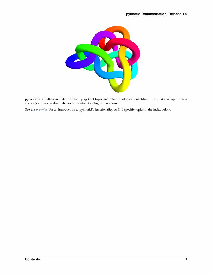
pyknotid is a Python module for identifying knot types and other topological quantities. It can take as input space-curves (such as visualised above) or standard topological notations.

See the overview for an introduction to pyknotid’s functionality, or find specific topics in the index below.

Contents 1


2 Contents

CHAPTER 1

Contents

1.1 Overview

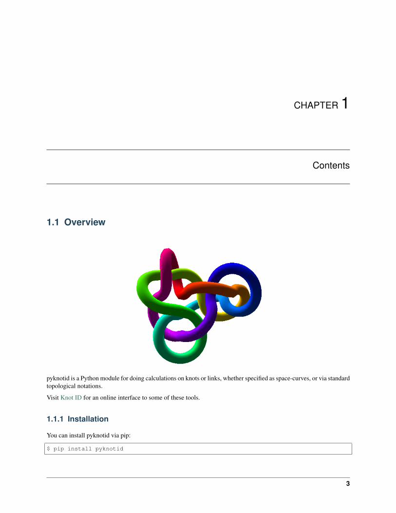
pyknotid is a Python module for doing calculations on knots or links, whether specified as space-curves, or via standardtopological notations.

Visit Knot ID for an online interface to some of these tools.

1.1.1 Installation

You can install pyknotid via pip:

$ pip install pyknotid

3

http://inclem.net/knotidentifier


By default pyknotid will try to compile some cython modules, but if this fails (normally because cython is not installed)it will only print a message and continue without errors. This won’t impact your use of pyknotid except that the cythoncalculations would be, especially during space-curve analysis. If you want to use the improved speed of the cythonimplementations but did not initially install them, you should uninstall pyknotid, install cython, and reinstall pyknotid.

You can also install the pyknotid development version from github at https://github.com/SPOCKnots/pyknotid.

1.1.2 Space curve analysis

pyknotid can perform many calculations on space curves specified as a set of points, as well as plotting the curves inthree dimensions or in projection. See the space curve documentation for more information.

Some topological calculations can only be performed for relatively short, simple curves, but in general pyknotid canwork fine even for space-curves with many thousands of points.

Example:

from pyknotid.make import trefoilfrom pyknotid.spacecurves import Knot

k = Knot(trefoil())

k.determinant() # 3k.gauss_code() # 1+a,2-a,3+a,1-a,2+a,3-ak.identify() # [<Knot 3_1>]

1.1.3 Topological representations

pyknotid can accept input using several standard topological notations including the Gauss code, planar diagram orDowker-Thistlethwaite notation. You can then calculate topological invariants, or even reconstruct a 3D space curve.See the representation documentation for more information.

Example:

from pyknotid.representations import GaussCode, Representation

gc = GaussCode('1+a,2-a,3+a,1-a,2+a,3-a')gc.simplify() # does nothing here, as no Reidemeister moves can be

# performed to immediately simplify the curve

# Representation is a generic topological representation providing# more methodsrep = Representation(gc)rep.determinant() # 3rep.space_curve() # <Knot with 34 points>, a space curve with the

# given Gauss code on projection

1.1.4 Knot catalogue

pyknotid can look up knot types in a prebuilt database containing various invariants for knots with up to 15 crossings.They can be looked up by the knot name (e.g. 3_1 for the trefoil knot, 4_1 for the figure-eight knot etc.), or the valuesof different knot invariants. See the knot catalogue documentation for more information.

Example:

4 Chapter 1. Contents

https://github.com/SPOCKnots/pyknotid


from pyknotid.catalogue import get_knot, from_invariants

k = get_knot('5_2')k.vassiliev_2 # 2k.determinant() # 3

k = get_knot('7_3').space_curve() # <Knot with 83 points>, a space curve# that forms a 7_3 knot.

knots = from_invariants(determinant=7, max_crossings=11) # [<Knot 5_2>,# <Knot 7_1>,# <Knot 9_42>,# <Knot K11n57>,# <Knot K11n96>,# <Knot K11n111>]

1.1.5 Example knots

pyknotid includes several functions for creating example knotted space curves. See the example knots documentationfor more details.

Example:

from pyknotid.make import torus_knot

k = torus_knot(p=5, q=2)k.identify() # [<Knot 5_1>]

from pyknotid.make import torus_link

l = torus_link(p=2, q=8) # a 2-component linkl.linking_number() # 8

from pyknotid.make import figure_eight

k = figure_eight()k.determinant() # 5

1.1. Overview 5


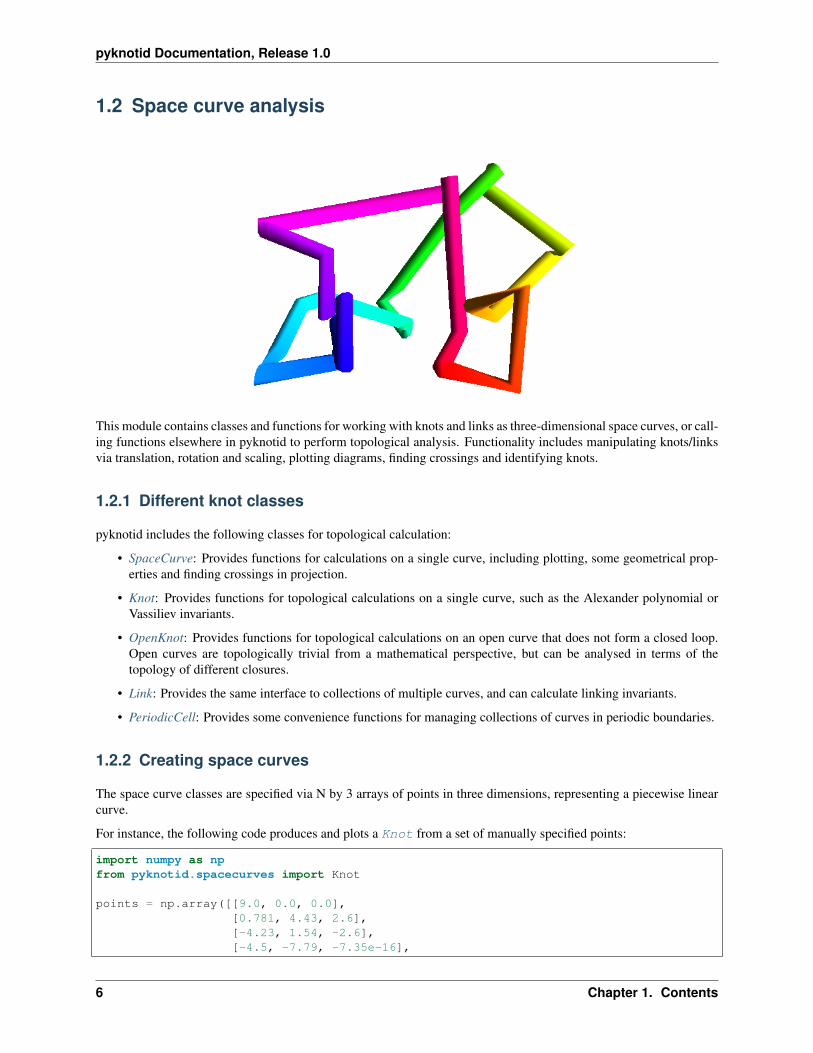
1.2 Space curve analysis

This module contains classes and functions for working with knots and links as three-dimensional space curves, or call-ing functions elsewhere in pyknotid to perform topological analysis. Functionality includes manipulating knots/linksvia translation, rotation and scaling, plotting diagrams, finding crossings and identifying knots.

1.2.1 Different knot classes

pyknotid includes the following classes for topological calculation:

• SpaceCurve: Provides functions for calculations on a single curve, including plotting, some geometrical prop-erties and finding crossings in projection.

• Knot: Provides functions for topological calculations on a single curve, such as the Alexander polynomial orVassiliev invariants.

• OpenKnot: Provides functions for topological calculations on an open curve that does not form a closed loop.Open curves are topologically trivial from a mathematical perspective, but can be analysed in terms of thetopology of different closures.

• Link: Provides the same interface to collections of multiple curves, and can calculate linking invariants.

• PeriodicCell: Provides some convenience functions for managing collections of curves in periodic boundaries.

1.2.2 Creating space curves

The space curve classes are specified via N by 3 arrays of points in three dimensions, representing a piecewise linearcurve.

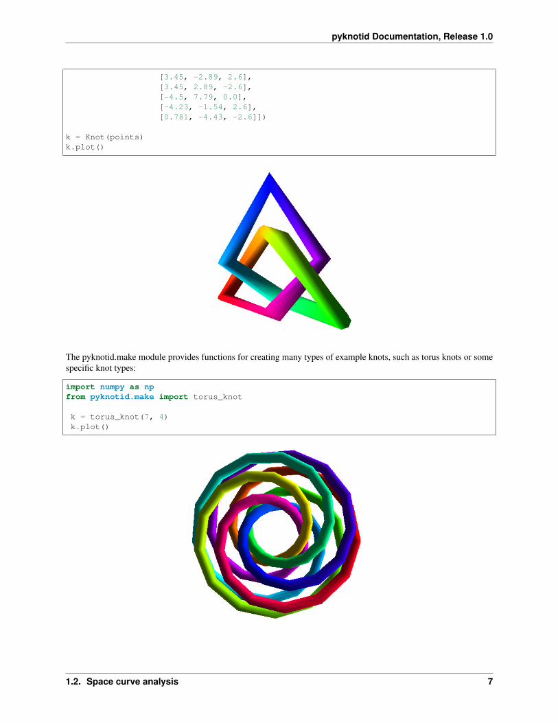
For instance, the following code produces and plots a Knot from a set of manually specified points:

import numpy as npfrom pyknotid.spacecurves import Knot

points = np.array([[9.0, 0.0, 0.0],[0.781, 4.43, 2.6],[-4.23, 1.54, -2.6],[-4.5, -7.79, -7.35e-16],



[3.45, -2.89, 2.6],[3.45, 2.89, -2.6],[-4.5, 7.79, 0.0],[-4.23, -1.54, 2.6],[0.781, -4.43, -2.6]])

k = Knot(points)k.plot()

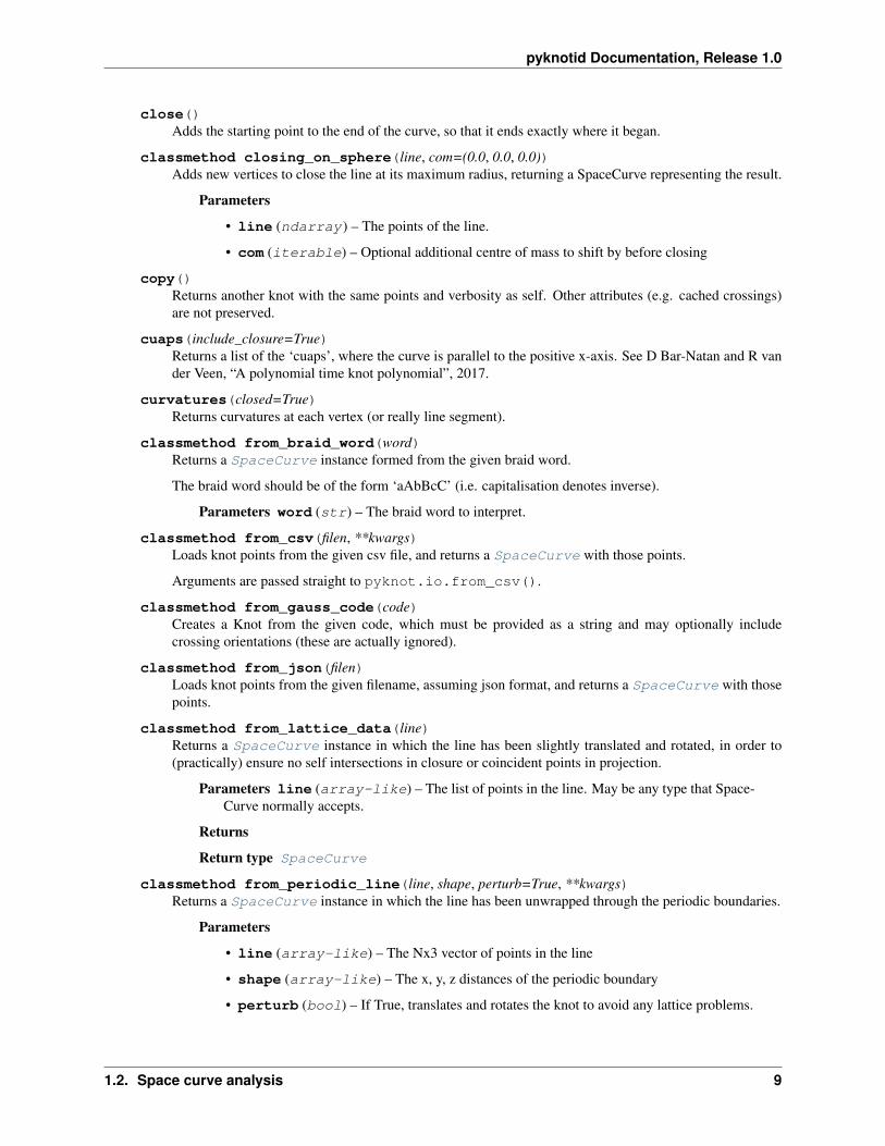
The pyknotid.make module provides functions for creating many types of example knots, such as torus knots or somespecific knot types:

import numpy as npfrom pyknotid.make import torus_knot

k = torus_knot(7, 4)k.plot()

1.2. Space curve analysis 7


1.2.3 SpaceCurve

The SpaceCurve class is the base for all space-curve analysis in pyknotid. It provides methods for geometricalmanipulation (translation, rotation etc.), calculating geometrical characteristics such as the writhe, and obtaining topo-logical representations of the curve by analysing its crossings in projection.

pyknotid provides other classes for topological analysis of the curves:

• Knot for calculating knot invariants of the space-curve.

• Link to handle multiple SpaceCurves and calculate linking invariants.

• Cell for handling multiple space-curves in a box with periodic boundaries.

API documentation

class pyknotid.spacecurves.spacecurve.SpaceCurve(points, verbose=True,add_closure=False,zero_centroid=False)

Bases: object

Class for holding the vertices of a single line, providing helper methods for convenient manipulation and analy-sis.

The methods of this class are largely geometrical (though this includes listing the crossings in projection andextracting a Gauss code etc.). For topological measurements, you should use a Knot.

This class deliberately combines methods to do many different kinds of measurements or manipulations. Someof these are externally available through other modules in pyknotid - if so, this is usually indicated in the methoddocstrings.

Parameters

• points (array-like) – The 3d points (vertices) of a piecewise linear curve representa-tion

• verbose (bool) – Indicates whether the SpaceCurve should print information duringprocessing

• add_closure (bool) – If True, adds a final point to the knot near to the start point, sothat it will appear visually to close when plotted.

• zero_centroid (bool) – If True, shifts the coordinates of the points so that their centreof mass is at the origin.

arclength(include_closure=True)Returns the arclength of the line, the sum of lengths of each piecewise linear segment.

Parameters include_closure (bool) – Whether to include the distance between the finaland first points. Defaults to True.

average_crossing_number(samples=10, recalculate=False, **kwargs)The (approximate) average crossing number of the space curve, obtained by averaging the planar writheover the given number of directions.

Parameters

• samples (int) – The number of directions to average over.

• recalculate (bool) – Whether to recalculate the ACN.

• **kwargs – These are passed directly to raw_crossings().



close()Adds the starting point to the end of the curve, so that it ends exactly where it began.

classmethod closing_on_sphere(line, com=(0.0, 0.0, 0.0))Adds new vertices to close the line at its maximum radius, returning a SpaceCurve representing the result.

Parameters

• line (ndarray) – The points of the line.

• com (iterable) – Optional additional centre of mass to shift by before closing

copy()Returns another knot with the same points and verbosity as self. Other attributes (e.g. cached crossings)are not preserved.

cuaps(include_closure=True)Returns a list of the ‘cuaps’, where the curve is parallel to the positive x-axis. See D Bar-Natan and R vander Veen, “A polynomial time knot polynomial”, 2017.

curvatures(closed=True)Returns curvatures at each vertex (or really line segment).

classmethod from_braid_word(word)Returns a SpaceCurve instance formed from the given braid word.

The braid word should be of the form ‘aAbBcC’ (i.e. capitalisation denotes inverse).

Parameters word (str) – The braid word to interpret.

classmethod from_csv(filen, **kwargs)Loads knot points from the given csv file, and returns a SpaceCurve with those points.

Arguments are passed straight to pyknot.io.from_csv().

classmethod from_gauss_code(code)Creates a Knot from the given code, which must be provided as a string and may optionally includecrossing orientations (these are actually ignored).

classmethod from_json(filen)Loads knot points from the given filename, assuming json format, and returns a SpaceCurve with thosepoints.

classmethod from_lattice_data(line)Returns a SpaceCurve instance in which the line has been slightly translated and rotated, in order to(practically) ensure no self intersections in closure or coincident points in projection.

Parameters line (array-like) – The list of points in the line. May be any type that Space-Curve normally accepts.

Returns

Return type SpaceCurve

classmethod from_periodic_line(line, shape, perturb=True, **kwargs)Returns a SpaceCurve instance in which the line has been unwrapped through the periodic boundaries.

Parameters

• line (array-like) – The Nx3 vector of points in the line

• shape (array-like) – The x, y, z distances of the periodic boundary

• perturb (bool) – If True, translates and rotates the knot to avoid any lattice problems.



gauss_code(recalculate=False, **kwargs)Returns a GaussCode instance representing the crossings of the knot.

The GaussCode instance is cached internally. If you want to recalculate it (e.g. to get an unsimplifiedversion if you have simplified it), you should pass recalculate=True.

This method passes kwargs directly to raw_crossings(), see the documentation of that function forall options.

gauss_diagram(simplify=False, **kwargs)Returns a GaussDiagram instance representing the crossings of the knot.


interpolate(num_points, s=0, **kwargs)Replaces self.points with points from a B-spline interpolation.

This method uses scipy.interpolate.splprep. kwargs are passed to this function.

octree_simplify(runs=1, plot=False, rotate=True, obey_knotting=True, **kwargs)Simplifies the curve via the octree reduction of :module:‘pyknotid.simplify.octree‘.

Parameters

• runs (int) – The number of times to run the octree simplification. Defaults to 1.

• plot (bool) – Whether to plot the curve after each run. Defaults to False.

• rotate (bool) – Whether to rotate the space curve before each run. Defaults to True asthis can make things much faster.

• obey_knotting (bool) – Whether to not let the line pass through itself. Defaults toTrue as this is always what you want for a closed curve.

• **kwargs – Any remaining kwargs are passed to the pyknotid.simplify.octree.OctreeCell constructor.

planar_diagram(**kwargs)Returns a PlanarDiagram instance representing the crossings of the knot.


planar_second_order_writhe(**kwargs)The second order writhe (type 2, i1,i3,i2,i4) of the projection of the curve along the z axis.

planar_writhe(**kwargs)Returns the current planar writhe of the knot; the signed sum of crossings of the current projection.

The ‘true’ writhe is the average of this quantity over all projection directions, and is available from thewrithe() method.

Parameters **kwargs – These are passed directly to raw_crossings().

plot(mode=’auto’, clf=True, closed=False, **kwargs)Plots the line. See pyknotid.visualise.plot_line() for full documentation.

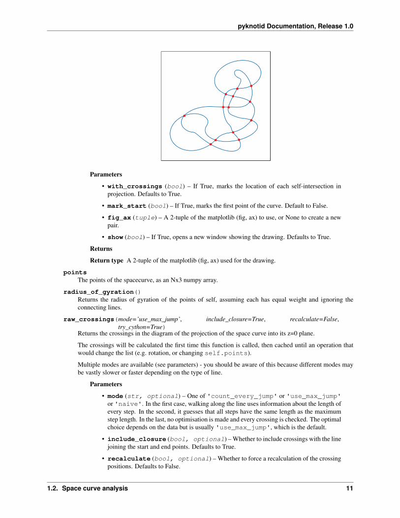
plot_projection(with_crossings=True, mark_start=False, fig_ax=None, show=True,mark_points=False)

Plots a 2D diagram of the knot projected along the current z-axis. The crossings, and start point of thecurve, can optionally be marked.

The projection is drawn using matplotlib.



Parameters

• with_crossings (bool) – If True, marks the location of each self-intersection inprojection. Defaults to True.

• mark_start (bool) – If True, marks the first point of the curve. Default to False.

• fig_ax (tuple) – A 2-tuple of the matplotlib (fig, ax) to use, or None to create a newpair.

• show (bool) – If True, opens a new window showing the drawing. Defaults to True.

Returns

Return type A 2-tuple of the matplotlib (fig, ax) used for the drawing.

pointsThe points of the spacecurve, as an Nx3 numpy array.

radius_of_gyration()Returns the radius of gyration of the points of self, assuming each has equal weight and ignoring theconnecting lines.

raw_crossings(mode=’use_max_jump’, include_closure=True, recalculate=False,try_cython=True)

Returns the crossings in the diagram of the projection of the space curve into its z=0 plane.

The crossings will be calculated the first time this function is called, then cached until an operation thatwould change the list (e.g. rotation, or changing self.points).

Multiple modes are available (see parameters) - you should be aware of this because different modes maybe vastly slower or faster depending on the type of line.

Parameters

• mode (str, optional) – One of 'count_every_jump' or 'use_max_jump'or 'naive'. In the first case, walking along the line uses information about the length ofevery step. In the second, it guesses that all steps have the same length as the maximumstep length. In the last, no optimisation is made and every crossing is checked. The optimalchoice depends on the data but is usually 'use_max_jump', which is the default.

• include_closure (bool, optional) – Whether to include crossings with the linejoining the start and end points. Defaults to True.

• recalculate (bool, optional) – Whether to force a recalculation of the crossingpositions. Defaults to False.



• try_cython (bool, optional) – Whether to force the use of the python (as op-posed to cython) implementation of find_crossings. This will make no difference if thecython could not be loaded, in which case python is already used automatically. Defaultsto True.

Returns The raw array of floats representing crossings, of the form [[line_index, other_index,+-1, +-1], . . . ], where the line_index and other_index are in arclength parameterised by in-tegers for each vertex and linearly interpolated, and the +-1 represent over/under and clock-wise/anticlockwise respectively.

Return type array-like

reparameterised(mode=’arclength’, num_points=None, interpolation=’linear’)Returns a new SpaceCurve where new points have been selected by interpolating the current ones.

Warning: This doesn’t do what you expect! The new segments will probably not all be separated bythe right amount in terms of the new parameterisation.

Parameters

• mode (str) – The function to reparameterise by. Defaults to ‘arclength’, which is cur-rently the only option.

• num_points (int) – The number of points in the new parameterisation. Defaults toNone, which means the same as the current number.

• interpolation (str) – The type of interpolation to use, passed directly to the kindoption of scipy.interpolate.interp1d. Defaults to ‘linear’, and other optionshave not been tested.

representation(recalculate=False, **kwargs)Returns a Representation instance representing the crossings of the knot.

The Representation instance is cached internally. If you want to recalculate it (e.g. to get an unsimplifiedversion if you have simplified it), you should pass recalculate=True.


rotate(angles=None)Rotates all the points of self by the given angles in each axis.

Parameters angles (array-like) – The rotation angles about x, y and z. If None, randomangles are used. Defaults to None.

scale(factor)Scales all the points of self by the given factor.

You can accomplish the same thing, or other more subtle transformations, by modifying self.:py:attr:points.

segment_arclengths()Returns an array of arclengths of every step in the line defined by self.points.

simplify_straight_segments(closed=False)Replaces successive curve segments with identical tangents with a single longer segment.

smooth(repeats=1, periodic=True, window_len=10, window=’hanning’)Smooths each of the x, y and z components of self.points by convolving with a window of the given typeand size.



Warning: This is not topologically safe, it can change the knot type of the curve. For topologicallysafe reduction, see octree_simplify().

Parameters

• repeats (int) – Number of times to run the smoothing algorithm. Defaults to 1.

• periodic (bool) – If True, the convolution window wraps around the curve. Defaultsto True.

• window_len (int) – Width of the convolution window. Defaults to 10. Passed topyknotid.spacecurves.smooth.smooth().

• window (string) – The type of convolution window. Defaults to ‘hanning’. Passed topyknotid.spacecurves.smooth.smooth().

to_json(filen)Writes the knot points to the given filename, in a json format that can be read later by SpaceCurve.from_json(). Uses pyknotid.io.to_json_file() internally.

to_txt(filen)Writes the knot points to the given filename, formatted with each x,y,z component of each point space-separated on its own line, i.e.:

...1.2 6.1 98.56.19 8.5 1.9...

torsions(signed=False, closed=True)Returns torsions at each vertex.

translate(vector)Translates all the points of self by the given vector.

Parameters vector (array-like) – The x, y, z translation distances

writhe(samples=10, recalculate=False, method=’integral’, include_acn=False, **kwargs)The (approximate) writhe of the space curve, obtained by averaging the planar writhe over the givennumber of directions.

Parameters

• samples (int) – The number of directions to average over. Defaults to 10.

• recalculate (bool) – Whether to recalculate the writhe even if a cached result isavailable. Defaults to False.

• method (str) – If ‘projections’, averages the planar writhe over many projections. If‘integral’, calculates the writhing integral.


zero_centroid()Translate such that the centroid (average position of vertices) is at (0, 0, 0).

1.2.4 Knot

Class for dealing with curves as knots. Knot provides many methods for topological manipulation and calculations.



API documentation

class pyknotid.spacecurves.knot.Knot(points, verbose=True, add_closure=False,zero_centroid=False)

Bases: pyknotid.spacecurves.spacecurve.SpaceCurve

Class for holding the vertices of a single line, providing helper methods for convenient manipulation and analy-sis.

A Knot just represents a single space curve, it may be topologically trivial!

This class deliberately combines methods to do many different kinds of measurements or manipulations. Someof these are externally available through other modules in pyknotid - if so, this is usually indicated in the methoddocstrings.

Parameters

• points (array-like) – The 3d points (vertices) of a piecewise linear curve representa-tion

• verbose (bool) – Indicates whether the Knot should print information during processing

• add_closure (bool) – If True, adds a final point to the knot near to the start point, sothat it will appear visually to close when plotted.

alexander_at_root(root, round=True, **kwargs)Returns the Alexander polynomial at the given root of unity, i.e. evaluated at exp(2 pi I / root).

The result returned is the absolute value.

Parameters

• root (int) – The root of unity to use, i.e. evaluating at exp(2 pi I / root). If this isiterable, this method returns a list of the results at every value of that iterable.

• round (bool) – If True and n in (1, 2, 3, 4), the result will be rounded to the nearestinteger for convenience, and returned as an integer type.

• **kwargs – These are passed directly to alexander_polynomial().

alexander_polynomial(variable=-1, quadrant=’lr’, mode=’python’, **kwargs)Returns the Alexander polynomial at the given point, as calculated by pyknotid.invariants.alexander().

See pyknotid.invariants.alexander() for the meanings of the named arguments.

copy()Returns another knot with the same points and verbosity as self. Other attributes (e.g. cached crossings)are not preserved.

determinant()Returns the determinant of the knot. This is the Alexander polynomial evaluated at -1.

exterior_manifold()The knot complement manifold of self as a SnapPy class giving access to all of SnapPy’s tools.

This method requires that Spherogram, and possibly SnapPy, are installed.

hyperbolic_volume()Returns the hyperbolic volume at the given point, via pyknotid.representations.PlanarDiagram.as_spherogram().

Returns

• volume (float) – A float representing the volume returned.



• accuracy (int) – The number of digits of precision. This is significant digits, e.g. 0.00021with 1 digit precision = 2E-4.

• solution_type (str) – The solution type of the manifold. Normally one of: - ‘containsdegenerate tetrahedra’ => may not be a valid result - ‘all tetrahedra positively oriented’ =>

really probably hyperbolic

identify(determinant=True, alexander=False, roots=(2, 3, 4), min_crossings=True)Provides a simple interface to pyknotid.catalogue.identify.from_invariants(), bypassing the given invariants. This does not support all invariants available, or more sophisticated iden-tification methods, so don’t be afraid to use the catalogue functions directly.

Parameters

• determinant (bool) – If True, uses the knot determinant in the identification. Defaultsto True.

• alexander (bool) – If True-like, uses the full alexander polynomial in the iden-tification. If the input is a dictionary of kwargs, these are passed straight toself.alexander_polynomial.

• roots (iterable) – A list of roots of unity at which to evaluate. Defaults to (2, 3,4), the first of which is redundant with the determinant. Note that higher roots can becalculated, but aren’t available in the database.

• min_crossings (bool) – If True, the output is restricted to knots with fewer crossingsthan the current projection of this one. Defaults to True. The only reason to turn thisoff is to see what other knots have the same invariants, it is never not useful for directidentification.

isolate_knot()Return indices of self.points within which the knot (if any) appears to lie, according to a simple closurealgorithm.

This method is experimental and may not provide very good results.

planar_writhe_quantities(num_angles=100, **kwargs)Returns the second order writhes, and arnold 2St+J+ values, for a range of different projection directions.

plot_isolated(**kwargs)Plots the curve in red, except for the isolated local knot which is coloured blue. The local knot is foundwith self.isolate_knot, which may not be reliable or have good resolution.

Parameters **kwargs – kwargs are passed directly to Knot.plot().


slipknot_alexander(num_samples=0, **kwargs)

Parameters

• num_samples (int) – The number of indices to cut at. Defaults to 0, which means tosample at all indices.

• **kwargs – Keyword arguments, passed directly to:meth:‘pyknotid.spacecurves.openknot.OpenKnot.alexander_fractions.

vassiliev_degree_2(simplify=True, **kwargs)Returns the Vassiliev invariant of degree 2 for the Knot.

Parameters



• simplify (bool) – If True, simplifies the Gauss code of self before calculating theinvariant. Defaults to True, but will work fine if you set it to False (and might even befaster).

• **kwargs – These are passed directly to gauss_code().

vassiliev_degree_3(simplify=True, try_cython=True, **kwargs)Returns the Vassiliev invariant of degree 3 for the Knot.

Parameters


• try_cython (bool) – Whether to try and use an optimised cython version of the routine(takes about 1/3 of the time for complex representations). Defaults to True, but the pythonfallback will be slower than setting it to False if the cython function is not available.


whitney_index()The degree of the Gauss map mapping a point on the curve to the direction of the positive tangent vectorat this point.

1.2.5 OpenKnot

Class for working with open (linear) curves, that do not form closed loops. OpenKnot provides methods for visual-ising these curves and analysing their topology via different kinds of closures.

API documentation

class pyknotid.spacecurves.openknot.OpenKnot(*args, **kwargs)Bases: pyknotid.spacecurves.spacecurve.SpaceCurve

Class for holding the vertices of a single line that is assumed to be an open curve. This class inherits fromSpaceCurve, replacing any default arguments that assume closed curves, and providing methods for statisticalanalysis of knot invariants on projection and closure.

All knot invariant methods return the results of a sampling over many projections of the knot, unless indicatedotherwise.

alexander_fractions(number_of_samples=10, **kwargs)Returns each of the Alexander polynomials from self.alexander_polynomials, with the fraction of thattype.

alexander_polynomials(number_of_samples=10, radius=None, recalculate=False,zero_centroid=False, optimise_closure=True)

Returns a list of Alexander polynomials for the knot, closing on a sphere of the given radius, with the givennumber of sample points approximately evenly distributed on the sphere.

The results are cached by number of samples and radius.

Parameters

• number_of_samples (int) – The number of points on the sphere to sample. Defaultsto 10.

• optimise_closure (bool) – If True, doesn’t really close on a sphere but at infinity.This lets the calculation be optimised slightly, and so is the default.



• radius (float) – The radius of the sphere on which to close the knot. Defaults toNone, which picks 10 times the largest Cartesian deviation from 0. This is only used ifoptimise_closure=False.

• zero_centroid (bool) – Whether to first move the average position of vertices to (0,0, 0). Defaults to True.

Returns A number_of_samples by 3 array of angles and alexander polynomials.

Return type ndarray

alexander_polynomials_multiroots(number_of_samples=10, radius=None,zero_centroid=False)

Returns a list of Alexander polynomials for the knot, closing on a sphere of the given radius, with the givennumber of sample points approximately evenly distributed on the sphere. The Alexander polynomials arefound at three different roots (2, 3 and 4) and a the knot types corresponding to these roots are returnedalso.

The results are cached by number of samples and radius.

Parameters

• number_of_samples (int) – The number of points on the sphere to sample. Defaultsto 10.

• radius (float) – The radius of the sphere on which to close the knot. Defaults toNone, which picks 10 times the largest Cartesian deviation from 0.

• zero_centroid (bool) – Whether to first move the average position of vertices to (0,0, 0). Defaults to True.

Returns A number_of_samples by 3 array of angles and alexander polynomials.

Return type ndarray

arclength()Calls pyknotid.spacecurves.spacecurve.SpaceCurve.arclength(), automatically notincluding the closure.

closing_distance()Returns the distance between the first and last points.

closure_alexander_polynomial(theta=0, phi=0)Returns the Alexander polynomial of the knot, when projected in the z plane after rotating the given thetaand phi to the North pole.

Parameters

• theta (float) – The sphere angle theta

• phi (float) – The sphere angle phi

generalised_alexander()Returns the generalised Alexander polynomial for the default projection of the open knot

multiroots_fractions(number_of_samples=10, **kwargs)Returns each of the knot types from self.alexander_polynomials_multiroots, with the fraction of that type.

plot_alexander_map(number_of_samples=10, scatter_points=False, mode=’imshow’, interpola-tion=100, **kwargs)

Creates (and returns) a projective diagram showing each different Alexander polynomial in a differentcolour according to a closure on a far away point in this direction.

Parameters



• number_of_samples (int) – The number of points on the sphere to close at.

• scatter_points (bool) – If True, plots a dot at each point on the map projectionwhere a closure was made.

• mode (str) – ‘imshow’ to plot the pixels of an image, otherwise plots filled contours.Defaults to ‘imshow’.

• interpolation (int) – The (short) side length of the interpolation grid on which themap projection is made. Defaults to 100.

plot_alexander_shell(number_of_samples=100, mode=’mesh’, radius=None, **kwargs)Plots the curve in 3d via self.plot(), along with a translucent sphere coloured by the type of knot obtainedby closing on each point.

Parameters are all passed to OpenKnot.alexander_polynomials(), except opacity and kwargswhich are given to mayavi.mesh, and sphere_radius_factor which gives the radius of the enclosing spherein terms of the maximum Cartesian distance of any point in the line from the origin.

plot_projections(number_of_samples)Plots the projection of the knot at each of the given number of samples squared, rotated such that thesample direction is vertical.

The output (and return) is a matplotlib plot with number_of_samples x number_of_samples axes.

plot_self_linking_map(number_of_samples=10, scatter_points=False, mode=’imshow’,**kwargs)

Creates (and returns) a projective diagram showing each different self linking number in a different colouraccording to a projection in this direction.

plot_self_linking_shell(number_of_samples=100, **kwargs)Plots the curve in 3d via self.plot(), along with a translucent sphere coloured by the self linking numberobtained by projecting from this point.

Parameters are all passed to OpenKnot.virtual_checks(), except opacity and kwargs which aregiven to mayavi.mesh, and sphere_radius_factor which gives the radius of the enclosing sphere in terms ofthe maximum Cartesian distance of any point in the line from the origin.

plot_virtual_map(number_of_samples=10, scatter_points=False, mode=’imshow’, **kwargs)Creates (and returns) a projective diagram showing each different virtual Boolean in a different colouraccording to a projection in this direction.

plot_virtual_shell(number_of_samples=10, zero_centroid=False, sphere_radius_factor=2.0,opacity=0.3, **kwargs)

Plots the curve in 3d via self.plot(), along with a translucent sphere coloured according to whether or notthe projection from this point corresponds to a virtual knot or not.

Parameters are all passed to OpenKnot.virtual_checks(), except opacity and kwargs which aregiven to mayavi.mesh, and sphere_radius_factor which gives the radius of the enclosing sphere in terms ofthe maximum Cartesian distance of any point in the line from the origin.


projection_invariant(**kwargs)First checks if the projection of an open curve is virtual or classical. If virtual, a virtual knot invariant iscalculated. Otherwise a classical invariant is calculated.

raw_crossings(mode=’use_max_jump’, virtual_closure=False, recalculate=False,try_cython=False)

Calls pyknotid.spacecurves.spacecurve.SpaceCurve.raw_crossings(), but withoutincluding the closing line between the last and first points (i.e. setting include_closure=False).



self_linking(theta=0, phi=0)Takes an open curve, finds its Gauss code (for the default projection) and calculates its self linking number,J(K). See Kauffman 2004 for more information.

Returns The self linking number of the open curve

Return type self_link_counter : int

self_linking_fractions(number_of_samples=10, **kwargs)Returns each of the self linking numbers from self.virtual.self_link.projections, with the fraction of eachtype.

self_linkings(number_of_samples=10, zero_centroid=False, **kwargs)Returns a list of self linking numbers for the curve with a given number of projections taken from directionsapproximately evenly distributed.

Parameters

• number_of_samples (int) – The number of points on the sphere to project from.Defaults to 10.

• zero_centroid (bool) – Whether to first move the average position of vertices to (0,0, 0). Defaults to False.

Returns A number_of_samples by 3 array of angles and self linking number

Return type ndarray

smooth(repeats=1, window_len=10, window=’hanning’)Calls pyknotid.spacecurves.spacecurve.SpaceCurve.smooth(), with the periodic argu-ment automatically set to False.

vassiliev_degree_2_average(samples=10, recalculate=False, **kwargs)Returns the average Vassliev degree 2 invariant calculated by averaging its combinatorial value over manydifferent projection directions.

Parameters

• samples (int) – The number of directions to average over. Defaults to 10.

• recalculate (bool) – Whether to recalculate the writhe even if a cached result isavailable. Defaults to False.


virtual_check()Takes an open curve and checks (for the default projection) if its Gauss code corresponds to a virtual knotor not. Returns a Boolean of this information.

Warning: This only checks the distance by which entries in the Gauss code are separated, it is notguaranteed to detect virtual knots.

Returns virtual – True if the Gauss code corresponds to a virtual knot. False otherwise.

Return type bool

virtual_checks(number_of_samples=10, zero_centroid=False)Returns a list of virtual Booleans for the curve with a given number if projections taken from directionsapproximately evenly distributed. A value of True corresponds to the projection giving a virtual knot, withFalse returned otherwise.



Parameters

• number_of_samples (int) – The number of points on the sphere to project from.Defaults to 10.

• zero_centroid (bool) – Whether to first move the average position of vertices to (0,0, 0). Defaults to False.

Returns A number_of_samples by 3 array of angles and virtual Booleans (True if virtual, Falseotherwise)

Return type ndarray

virtual_fractions(number_of_samples=10, **kwargs)Returns each of the virtual booleans from self.virtual.check.projections, with the fraction of each type.

pyknotid.spacecurves.openknot.gall_peters(theta, phi)Converts spherical coordinates to the Gall-Peters projection of the sphere, an area-preserving projection in theshape of a Rectangle.

Parameters

• theta (float) – The latitude, in radians.

• phi (float) – The longitude, in radians.

pyknotid.spacecurves.openknot.knot_db_to_string(database_object)Takes output from from_invariants() and returns knot type as decimal. For example: <Knot 3_1> becomes 3.1and <Knot K13n1496> becomes 13.1496

pyknotid.spacecurves.openknot.mollweide(phi, lambda_)Converts spherical coordinates to the Mollweide projection of the sphere, an area-preserving projection in theshape of an ellipse.

Parameters

• phi (float) – The latitude, in radians.

• lambda (float) – The longitude, in radians.

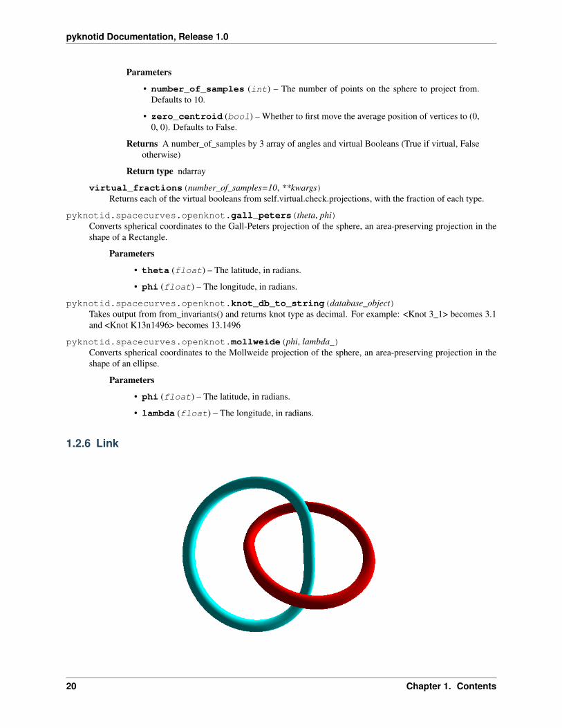
1.2.6 Link



Class for dealing with multiple curves as a link. Link provides methods for topological manipulation and calculationson multiple curves.

API documentation

class pyknotid.spacecurves.link.Link(lines, verbose=True)Bases: object

Class for holding the vertices of multiple lines, providing helper methods for convenient manipulation andanalysis.

The data is stored internally as multiple :class:‘Knot‘s.

Parameters

• lines (list of nx3 array-like or Knots) – List with the points of each line.

• verbose (bool) – Whether to print information during processing. Defaults to True.

arclength(include_closures=True)Returns the sum of arclengths of the lines.

Parameters include_closures (bool) – Whether to include the distance between the finaland first points of each line. Defaults to True.

classmethod from_periodic_lines(lines, shape, perturb=True)Returns a Link instance in which the lines have been unwrapped through the periodic boundaries.

Parameters

• line (list) – A list of the Nx3 vectors of points in the lines

• shape (array-like) – The x, y, z distances of the periodic boundary

• perturb (bool) – If True, translates and rotates the knot to avoid any lattice problems.

gauss_code(**kwargs)Returns a GaussCode instance representing the crossings of the knot.

The GaussCode instance is cached internally. If you want to recalculate it (e.g. to get an unsimplifiedversion if you have simplified it), you should pass recalculate=True.


linking_number(**kwargs)Returns the linking number of the lines in the Link, the sum of signed crossings between them, ignoringcrossings of a line with itself.

octree_simplify(runs=1, plot=False, rotate=True, obey_knotting=False, **kwargs)Simplifies the curves via the octree reduction of :module:‘pyknotid.simplify.octree‘.

Parameters

• runs (int) – The number of times to run the octree simplification. Defaults to 1.

• plot (bool) – Whether to plot the curve after each run. Defaults to False.

• rotate (bool) – Whether to rotate the space curve before each run. Defaults to True asthis can make things much faster.

• obey_knotting (bool) – Whether to not let the line pass through itself. Defaults toFalse - knotting of individual components will be ignored! This is much faster than thealternative.



:param kwargs are passed to the pyknotid.simplify.octree.OctreeCell: :param constructor.:

plot(mode=’vispy’, clf=True, colours=None, **kwargs)Plots all the lines. See pyknotid.visualise.plot_line() for full documentation.

raw_crossings(mode=’use_max_jump’, only_with_other_lines=True, include_closures=True, re-calculate=False, try_cython=True)

Returns the crossings in the diagram of the projection of the space curve into its z=0 plane.

The crossings will be calculated the first time this function is called, then cached until an operation thatwould change the list (e.g. rotation, or changing self.points).

Multiple modes are available (see parameters) - you should be aware of this because different modes maybe vastly slower or faster depending on the type of line.

Parameters

• mode (str, optional) – One of 'count_every_jump' and'use_max_jump'. In the former case, walking along the line uses informationabout the length of every step. In the latter, it guesses that all steps have the same lengthas the maximum step length. The optimal choice depends on the data, but is usually'use_max_jump', which is the default.

• only_with_other_lines (bool) – If True, ignores self-crossings (i.e. the knot typeof the loops) and returns only a list of crossings between the loops. Defaults to True

• include_closures (bool, optional) – Whether to include crossings with thelines joining their start and end points. Defaults to True.

• recalculate (bool, optional) – Whether to force a recalculation of the crossingpositions. Defaults to False.

• try_cython (bool, optional) – Whether to try to use a cython implementation ofcrossing finding. This will make no difference if the cython could not be loaded, in whichcase python is already used automatically. Defaults to True.

Returns The raw array of floats representing crossings, of the form [[line_index, other_index,+-1, +-1], . . . ], where the line_index and other_index are in arclength parameterised by in-tegers for each vertex and linearly interpolated, and the +-1 represent over/under and clock-wise/anticlockwise respectively.

Return type array-like

rotate(angles=None)Rotates all the points of each line of self by the given angle in each axis.

Parameters angles (array-like) – Rotation angles about x, y and z axes. If None, randomangles are used. Defaults to None.

smooth(*args, **kwargs)Smooths each of the x, y and z components of each of self.lines by convolving with a window of the giventype and size.

kwargs are passed straight to pyknotid.spacecurves.spacecurve.SpaceCurve.smooth().

translate(vector, lines=None)Translate all points in some or all lines of self.

Parameters

• vector (array-like) – The x, y, z translation distances



• lines (list or int) – The list of line indices to which the translation should beapplied. Defaults to None, which applies the translation to all the lines of self. If aninteger is supplied, only the line with this index is translated.

1.2.7 PeriodicCell

Tools for working with a periodic cell of spacecurves.

API documentation

class pyknotid.spacecurves.periodiccell.Cell(lines, shape, periodic=True, cram=False,downsample=None)

Bases: object

Class for holding the vertices of some number of lines with periodic boundary conditions.

Parameters

• lines (list) – Must be a list of Knots or ndarrays of vertices.

• shape (tuble or int) – The shape of the cell, in whatever units the lines use.

• periodic (bool) – Whether the cell is periodic. If True, lines are marked as ‘nth’ or‘loop’ in self.line_types. Defaults to True.

classmethod from_qwer(qwer, shape, **kwargs)Returns an instance of Cell from a quartet of differently classified lines in periodic boundaries.

Parameters

• qwer (tuple) – Should be a 4-tuple of lists q, w, e, r. q is closed loops, w is lineswith non-trivial homology, e is lines that terminate on the boundaries of the cell, r is anyremaining (unclassified) lines.

• shape (int or tuple) – The size of the cell along each axis. If a single number ispassed, all axes are assumed to be the same length.

linking_matrix()Get the linking numbers of each line in the cell with every other.

smooth(repeats=1, window_len=10)Smooth each line in the curve, equivalent to smooth().

1.3 Invariants

Functions for retrieving invariants of knots and links.

Many of these functions can be called in a more convenient way via methods of the space curve classes (e.g. Knot)or the Representation class.

1.3.1 Mathematica

Functions whose name ends with _mathematica try to create an external Mathematica process to calculate theanswer. They may hang or have other problems if Mathematica isn’t available in your $PATH, so be careful usingthem.

1.3. Invariants 23


Warning: This module may be broken into multiple components at some point.

1.3.2 API documentation

pyknotid.invariants.alexander(representation, variable=-1, quadrant=’lr’, simplify=True,mode=’python’)

Calculates the Alexander polynomial of the given knot. The representation must have just one knot component,or the calculation will fail or potentially give bad results.

The result is returned with whatever numerical precision the algorithm produces, it is not rounded.

The given representation must be simplified (RM1 performed if possible) for this to work, otherwise thematrix has overlapping elements. This is so important that this function automatically calls pyknotid.representations.gausscode.GaussCode.simplify(), you must disable this manually if youdon’t want to do it.

Note: If ‘maxima’ or ‘mathematica’ is chosen as the mode, the variable will automatically be set to t.

Note: If the mode is ‘cypari’, the quadrant argument will be ignored and the upper-left quadrant always used.

Parameters

• representation (Anything convertible to a) – GaussCode A pyknotidrepresentation class for the knot, or anything that can automatically be converted into aGaussCode (i.e. by writing GaussCode(your_object)).

• variable (float or complex or sympy variable) – The value to caltulatethe Alexander polynomial at. Defaults to -1, but may be switched to the sympy variable tin the future. Supports int/float/complex types (fast, works for thousands of crossings) orsympy expressions (much slower, works mostly only for <100 crossings).

• quadrant (str) – Determines what principal minor of the Alexander matrix should beused in the calculation; all choices should give the same answer. Must be ‘lr’, ‘ur’, ‘ul’ or‘ll’ for lower-right, upper-right, upper-left or lower-left respectively.

• simplify (bool) – Whether to call the GaussCode simplify method, defaults to True.

• mode (string) – One of ‘python’, ‘maxima’, ‘cypari’ or ‘mathematica’. denotes whattools to use; if python, the calculation is performed with numpy or sympy as appropriate. Ifmaxima or mathematica, that program is called by the function - this will only work if theexternal tool is installed and available. Defaults to python.

pyknotid.invariants.alexander_cypari(representation, quadrant=’ul’, verbose=False, sim-plify=True)

Returns the Alexander polynomial of the given representation, by calculating the matrix determinant via cypari,a python interface to Pari-GP.

The function only supports evaluating at the variable t.

The returned object is a cypari query type.

Parameters




• quadrant (str) – Determines what principal minor of the Alexander matrix should beused in the calculation; all choices should give the same answer. Must be ‘lr’, ‘ur’, ‘ul’ or‘ll’ for lower-right, upper-right,

• verbose (bool) – Whether to print information about the procedure. Defaults to False.

• simplify (bool) – If True, tries to simplify the representation before calculating thepolynomial. Defaults to True.

pyknotid.invariants.alexander_mathematica(representation, quadrant=’ul’, verbose=False,via_file=True)

Returns the Alexander polynomial of the given representation, by creating a Mathematica process and runningits knot routines. The Mathematica installation must include the KnotTheory package.


Parameters




• via_file (bool) – If True, calls Mathematica via a written filemathematicascript.m, otherwise calls Mathematica directly with runMath.The latter had a nasty bug in at least one recent Mathematica version, so the default is toTrue.


pyknotid.invariants.alexander_maxima(representation, quadrant=’ul’, verbose=False, sim-plify=True)

Returns the Alexander polynomial of the given representation, by calculating the matrix determinant in maxima.


Parameters





pyknotid.invariants.arnold_2St_2Jminus(representation)Returns J- + 2 * St where J+ and St are Arnold’s invariants of plane curves.

1.3. Invariants 25


See ‘Invariants of curves and fronts via Gauss diagrams’, M Polyak, Topology 37, 1998.

pyknotid.invariants.arnold_2St_2Jplus(representation)Returns J+ + 2 * St where J+ and St are Arnold’s invariants of plane curves.

The calculation is performed by transforming the representation into a representation of an unknot by flippingcrossings, then calculating the second order writhe.

See ‘Invariants of curves and fronts via Gauss diagrams’, M Polyak, Topology 37, 1998.

pyknotid.invariants.contract_points(planar_diagram)For appropriately contracting :class: Points in a :class: PlanarDiagram According to the following rules:

P_a,b P_b,c -> P_a,c P_a,b P_a,b -> P_a,a

pyknotid.invariants.hyperbolic_volume(representation)The hyperbolic volume, calculated by the SnapPy library for studying the topology and geometry of 3-manifolds.This function depends on the Spherogram module, distributed with SnapPy or available separately.

Parameters representation (A PlanarDiagram, or anything convertibleto a) – GaussCode A pyknotid representation class for the knot, or anything that canautomatically be converted into a GaussCode (i.e. by writing GaussCode(your_object)),or a PlanarDiagram.

pyknotid.invariants.jones_mathematica(representation)Returns the Jones polynomial of the given representation, by creating a Mathematica process and running itsknot routines. The Mathematica installation must include the KnotTheory package.

The function only supports evaluating at the variable q.

Parameters representation (A PlanarDiagram, or anything convertibleto a) – GaussCode A pyknotid representation class for the knot, or anything that canautomatically be converted into a GaussCode (i.e. by writing GaussCode(your_object)),or a PlanarDiagram.

pyknotid.invariants.second_order_writhe(representation)Returns the second order writhe (i1,i3,i2,i4) of the representation, as defined in Lin and Wang.

pyknotid.invariants.self_linking(representation)Returns the self linking number J(K) of the Gauss code, an invariant of virtual knots. See Kauffman 2004 formore information.

Currently only works for knots.

pyknotid.invariants.vassiliev_degree_2(representation)Calculates the Vassiliev invariant of degree 2 of the given knot. The representation must have just one knotcomponent, this doesn’t work for links.

Parameters representation (Anything convertible to a) – GaussCode A py-knotid representation class for the knot, or anything that can automatically be converted intoa GaussCode (i.e. by writing GaussCode(your_object)).

pyknotid.invariants.vassiliev_degree_3(representation, try_cython=True)Calculates the Vassiliev invariant of degree 3 of the given knot. The representation must have just one knotcomponent, this doesn’t work for links.

Parameters





pyknotid.invariants.virtual_vassiliev_degree_3(representation)Calculates the virtual Vassiliev invariant of degree 3 (for non-long-knots) of the given representation, as de-scribed in ‘Finite type invariants of classical and virtual knots’ by Goussarov, Polyak and Viro.

Parameters representation (Representation) – A representation class, or anything con-vertible to one (in principle).

1.4 Topological representations

Knots and links can be encoded in many different ways, generally by enumerating their self-intersections in projectionalong some axis. We provide here

This module contains classes and functions for representing knots in knot diagrams, mainly the pyknotid.representations.gausscode.GaussCode and pyknotid.representations.planardiagram.PlanarDiagram.

These provide convenient methods to convert between different representations, and to simplify via Reidemeistermoves.

1.4.1 Creating representations

Knot representations can be calculated from space curves, or created directly by inputting standard notations.

From space curves

pyknotid’s space curve classes can all return topological representations. For instance:

from pyknotid.spacecurves import Knotfrom pyknotid.make import trefoilk = Knot(trefoil())

You can extract a GaussCode object:

k.gauss_code() # 1+a,2-a,3+a,1-a,2+a,3-a

or a PlanarDiagram:

k.planar_diagram() # PD with 3: X_{2,5,3,6} X_{4,1,5,2} X_{6,3,1,4}

or a Gauss diagram:

k.gauss_diagram() # plots the diagram in a new window using matplotlib

1.4. Topological representations 27


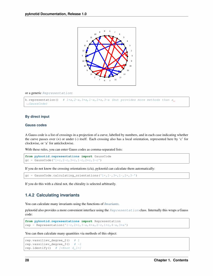
or a generic Representation:

k.representation() # 1+a,2-a,3+a,1-a,2+a,3-a (but provides more methods than a→˓GaussCode)

By direct input

Gauss codes

A Gauss code is a list of crossings in a projection of a curve, labelled by numbers, and in each case indicating whetherthe curve passes over (+) or under (-) itself. Each crossing also has a local orientation, represented here by ‘c’ forclockwise, or ‘a’ for anticlockwise.

With these rules, you can enter Gauss codes as comma-separated lists:

from pyknotid.representations import GaussCodegc = GaussCode('1+c,2-c,3+c,1-c,2+c,3-c')

If you do not know the crossing orientations (c/a), pyknotid can calculate them automatically:

gc = GaussCode.calculating_orientations('1+,2-,3+,1-,2+,3-')

If you do this with a chiral not, the chirality is selected arbitrarily.

1.4.2 Calculating invariants

You can calculate many invariants using the functions of Invariants.

pyknotid also provides a more convenient interface using the Representation class. Internally this wraps a Gausscode:

from pyknotid.representations import Representationrep = Representation('1-c,2+c,3-a,4+a,2-c,1+c,4-a,3+a')

You can then calculate many quantities via methods of this object:

rep.vassiliev_degree_2() # 1rep.vassiliev_degree_3() # -1rep.identify() # [<Knot 4_1>]



For a full list of available functions, see Representation.

1.4.3 GaussCode

Classes for working with Gauss codes representing planar projections of curves.

See class documentation for more details.

API documentation

class pyknotid.representations.gausscode.GaussCode(crossings=”, verbose=True)Bases: object

Class for containing and manipulating Gauss codes.

By default you must pass an extended Gauss code that includes the sign of each crossing (‘c’ for clockwise or ‘a’for anticlockwise), e.g. 1+c,2-c,3+c,1-c,2+c,3-c for the trefoil knot. If you do not know the crossingsigns you can instead call GaussCode.calculating_orientations(), e.g. gc = GaussCode.calculating_orientations('1+,2-,3+,1-,2+,3-').

The length of a Gauss code (e.g. len(GaussCode())) is the number of crossings in it.

Parameters

• crossings (array-like or string or PlanarDiagram or GaussCode)– A raw_crossings array from a Knot or Link, or a string representation of the form(e.g.) 1+c,2-c,3+c,1-c,2+c,3-c, with commas between entries, and with multiplelink components separated by spaces and/or newlines. If a PlanarDiagram or GaussCode ispassed, the code is duplicated.

• verbose (bool) – Whether to print information during calculations. Defaults to True.

classmethod calculating_orientations(code)Takes a Gauss code without crossing orientations and returns an equivalent Gauss code (though not neces-sarily of the same length).

This works by generating a space curve and finding its self-intersections on projection. This is overkill forthe problem, but works.

flipped()Returns a copy of self with crossing over/under switched.

mirrored()Returns a copy of self with crossing orientations reversed.

reindex_crossings()Replaces the indices of the crossings in the Gauss code with the integers from 1 to its length.

Note that this modifies the Gauss code in place, the previous indices are not recorded.

simplify(one=True, two=True, one_extended=True)Simplifies the GaussCode, performing the given Reidemeister moves everywhere possible, as many timesas possible, until the GaussCode is no longer changing.

This modifies the GaussCode - (non-topological) information may be lost!

Parameters

• one (bool) – Whether to use Reidemeister 1, defaults to True.



• two (bool) – Whether to use Reidemeister 2, defaults to True.

• one_extended (bool) – Whether to use extended Reidemeister 1, which removescrossings connected by arcs which include only over or only under crossings (and whichmust thus be topologically irrelevant). Defaults to True.

without_virtual()Returns a version of the Gauss code without explicit virtual crossings.

1.4.4 PlanarDiagram

Classes for working with planar diagram notation of knot diagrams.

See individual class documentation for more details.

API documentation

class pyknotid.representations.planardiagram.Crossing(a=None, b=None, c=None,d=None)

Bases: list

A single crossing in a planar diagram. Each PlanarDiagram is a list of these.

Parameters

• a (int or None) – The first entry in the list of lines meeting at this Crossing.

• b (int or None) – The second entry in the list of lines meeting at this Crossing.

• c (int or None) – The third entry in the list of lines meeting at this Crossing.

• d (int or None) – The fourth entry in the list of lines meeting at this Crossing.

as_mathematica()Get a string of mathematica code that can represent the Crossing in mathematica’s knot library.

The mathematica code won’t be valid if any lines of self are None.

Return type str

components()Returns a de-duplicated list of lines intersecting at this Crossing.

Return type list

update_line_number(old, new)Replaces all instances of the given line number in self.

Parameters

• old (int) – The old line number

• new (int) – The number to replace it with

valid()True if all intersecting lines are not None.

class pyknotid.representations.planardiagram.PlanarDiagram(crossings=”)Bases: list

A class for containing and manipulating planar diagrams.

Just provides convenient display and conversion methods for now. In the future, will support simplification.



Shorthand input may be of the form X_1,4,2,5 X_3,6,4,1 X_5,2,6,3. This is (should be?) the sameas returned by repr.

Parameters crossings (array-like or string or GaussCode) – The list of cross-ings in the diagram, which will be converted to an internal planar diagram representation. Cur-rently these are mostly converted via a GaussCode instance, so in addition to the shorthand anyarray-like supported by GaussCode may be used.

as_mathematica()Returns a mathematica code representation of self, usable in the mathematica knot tools.

as_networkx()Get a networkx graph representing the planar diagram, where each node is a crossing and each edge is anarc. This is a non-directed non-multi graph; where two arcs join the same crossing, they are represented asa single edge, but information about duplicates is returned alongside the graph.

Returns

• g (Graph) – The networkx graph

• duplicates (list) – A list of tuples representing nodes joined by multiple edges.

• heights (dict) – A dictionary of (start, end, arc_number) graph edges, containing the startand end height of each edge.

• first_edge (tuple) – The first edge in the graph, including (start, end, arc_number).

as_networkx_extended()(internal use only) Returns a networkx Graph along with extra information about the crossings.

as_spherogram()Get a planar diagram class from the Spherogram module, which can be used to access SnapPy’s manifoldtools.

This method requires that spherogram and SnapPy are installed.

pyknotid.representations.planardiagram.index_height(index)Returns the height based on the index of the crossing in an entry of a planar diagram; the 0th and 2nd indicesare under crossings, and the 1st and 3rd are over crossings.

pyknotid.representations.planardiagram.shorthand_to_crossings(s)Takes a planar diagram shorthand string, and returns a list of :class:‘Crossing‘s.



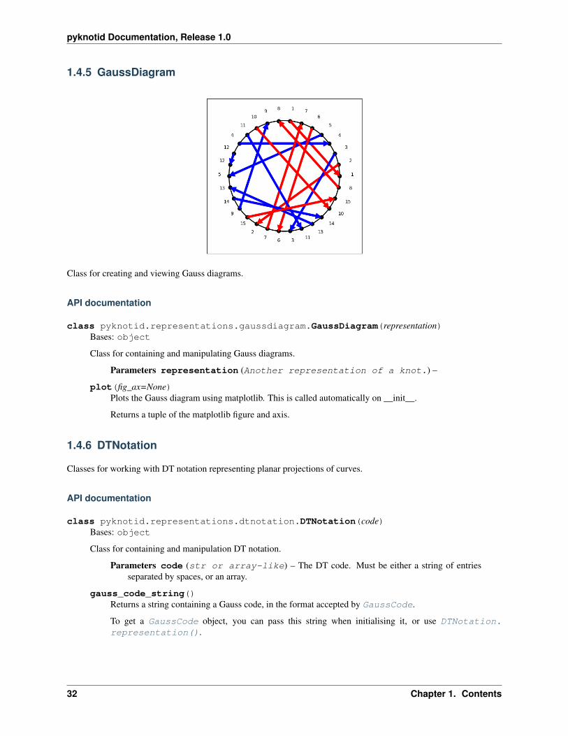
1.4.5 GaussDiagram

Class for creating and viewing Gauss diagrams.

API documentation

class pyknotid.representations.gaussdiagram.GaussDiagram(representation)Bases: object

Class for containing and manipulating Gauss diagrams.

Parameters representation (Another representation of a knot.) –

plot(fig_ax=None)Plots the Gauss diagram using matplotlib. This is called automatically on __init__.

Returns a tuple of the matplotlib figure and axis.

1.4.6 DTNotation

Classes for working with DT notation representing planar projections of curves.

API documentation

class pyknotid.representations.dtnotation.DTNotation(code)Bases: object

Class for containing and manipulation DT notation.

Parameters code (str or array-like) – The DT code. Must be either a string of entriesseparated by spaces, or an array.

gauss_code_string()Returns a string containing a Gauss code, in the format accepted by GaussCode.

To get a GaussCode object, you can pass this string when initialising it, or use DTNotation.representation().



representation(**kwargs)Returns a Representation representing the same DT code. The crossing orientations (and thereforeresulting chirality) are chosen arbitrarily.

1.4.7 Representation

An abstract representation of a Knot, providing methods for the calculation of topological invariants.

API documentation

class pyknotid.representations.representation.Representation(crossings=”,verbose=True)

Bases: pyknotid.representations.gausscode.GaussCode

An abstract representation of a knot or link. Internally this is just a Gauss code, but it exposes extra topologicalmethods and may in future be refactored to work differently.

alexander_at_root(root, round=True, **kwargs)Returns the Alexander polynomial at the given root of unity, i.e. evaluated at exp(2 pi I / root).

The result returned is the absolute value.

Parameters

• root (int) – The root of unity to use, i.e. evaluating at exp(2 pi I / root). If this isiterable, this method returns a list of the results at every value of that iterable.

• round (bool) – If True and n in (1, 2, 3, 4), the result will be rounded to the nearestinteger for convenience, and returned as an integer type.

• **kwargs – These are passed directly to alexander_polynomial().

alexander_polynomial(variable=-1, quadrant=’lr’, mode=’python’, force_no_simplify=False)Returns the Alexander polynomial at the given point, as calculated by pyknotid.invariants.alexander().

See pyknotid.invariants.alexander() for the meanings of the named arguments.

exterior_manifold()The knot complement manifold of self as a SnapPy class giving access to all of SnapPy’s tools.

This method requires that Spherogram, and possibly SnapPy, are installed.

hyperbolic_volume()Returns the hyperbolic volume at the given point, via pyknotid.representations.PlanarDiagram.as_spherogram().

identify(determinant=True, vassiliev_2=True, vassiliev_3=None, alexander=False, roots=(2, 3, 4),min_crossings=True)

Provides a simple interface to pyknotid.catalogue.identify.from_invariants(), bypassing the given invariants. This does not support all invariants available, or more sophisticated iden-tification methods, so don’t be afraid to use the catalogue functions directly.

Parameters

• determinant (bool) – If True, uses the knot determinant in the identification. Defaultsto True.

• alexander (bool) – If True-like, uses the full alexander polynomial in the iden-tification. If the input is a dictionary of kwargs, these are passed straight toself.alexander_polynomial.



• roots (iterable) – A list of roots of unity at which to evaluate. Defaults to (2, 3,4), the first of which is redundant with the determinant. Note that higher roots can becalculated, but aren’t available in the database.

• min_crossings (bool) – If True, the output is restricted to knots with fewer crossingsthan the current projection of this one. Defaults to True. The only reason to turn thisoff is to see what other knots have the same invariants, it is never not useful for directidentification.

• vassiliev_2 (bool) – If True, uses the Vassiliev invariant of order 2. Defaults toTrue.

• vassiliev_3 (bool) – If True, uses the Vassiliev invariant of order 3. Defaults toNone, which means the invariant is used only if the representation has less than 30 cross-ings.

is_virtual()Takes an open curve and checks (for the default projection) if its Gauss code corresponds to a virtual knotor not. Returns a Boolean of this information.

Returns virtual – True if the Gauss code corresponds to a virtual knot. False otherwise.

Return type bool

self_linking()Returns the self linking number J(K) of the Gauss code, an invariant of virtual knots. See Kauffman 2004for more information.

Returns slink_counter – The self linking number of the open curve

Return type int

vassiliev_degree_2(simplify=True)Returns the Vassiliev invariant of degree 2 for the Knot.

Parameters



vassiliev_degree_3(simplify=True, try_cython=True)Returns the Vassiliev invariant of degree 3 for the Knot.

Parameters




virtual_vassiliev_degree_3()Returns the virtual Vassiliev invariant of degree 3 for the representation.



1.5 Knot catalogue

pyknotid provides knot lookup by name or invariant values, using a prebuilt database.

The knot database includes information about all knots with up to 15 crossings, with topological invariants followingthose indexed by the Knot Atlas and the KnotInfo Table of Knot Invariants, or calculated by pyknotid using theDowker-Thistlethwaite codes of the knots.

1.5.1 Downloading the database

The database must normally be downloaded separately, and is currently approximately 230MB in size.

If you do not download the database, most of pyknotid will work fine. Only the explicit knot identification by databaselookup, or direct database queries, are not available.

To download the knot database:

from pyknotid.catalogue.getdb import download_databasedownload_database()

After this has completed (it may take a few seconds), the database functions should all work immediately.

For other database management functions, see Database download module.

1.5.2 Lookup by name

Use pyknotid.catalogue.identify.get_knot():

from pyknotid.catalogue.identify import get_knottrefoil = get_knot('3_1')figure_eight = get_knot('4_1')

1.5.3 Lookup by invariants

Use pyknotid.catalogue.identify.from_invariants():

from pyknotid.catalogue.identify import from_invariants

from_invariants(determinant=5, max_crossings=9)# returns [<Knot 4_1>, <Knot 5_1>]

import sympy as symt = sym.var('t')from_invariants(alexander=1-t+t**2, max_crossings=9)# returns [<Knot 3_1>]

For a full list of lookup parameters, see from_invariants().

1.5.4 Exploring properties of knots

You can view more properties of any knot returned by the database:

1.5. Knot catalogue 35

http://katlas.org/wiki/Main_Page

http://www.indiana.edu/~knotinfo/


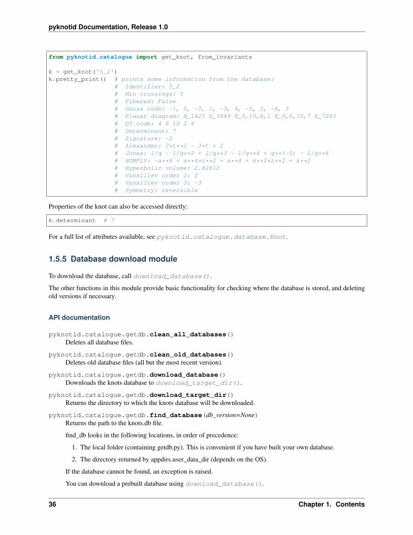
from pyknotid.catalogue import get_knot, from_invariants

k = get_knot('5_2')k.pretty_print() # prints some information from the database:

# Identifier: 5_2# Min crossings: 5# Fibered: False# Gauss code: -1, 5, -2, 1, -3, 4, -5, 2, -4, 3# Planar diagram: X_1425 X_3849 X_5,10,6,1 X_9,6,10,7 X_7283# DT code: 4 8 10 2 6# Determinant: 7# Signature: -2# Alexander: 2*t**2 - 3*t + 2# Jones: 1/q - 1/q**2 + 2/q**3 - 1/q**4 + q**(-5) - 1/q**6# HOMFLY: -a**6 + a**4*z**2 + a**4 + a**2*z**2 + a**2# Hyperbolic volume: 2.82812# Vassiliev order 2: 2# Vassiliev order 3: -3# Symmetry: reversible

Properties of the knot can also be accessed directly:

k.determinant # 7

For a full list of attributes available, see pyknotid.catalogue.database.Knot.

1.5.5 Database download module

To download the database, call download_database().

The other functions in this module provide basic functionality for checking where the database is stored, and deletingold versions if necessary.

API documentation

pyknotid.catalogue.getdb.clean_all_databases()Deletes all database files.

pyknotid.catalogue.getdb.clean_old_databases()Deletes old database files (all but the most recent version).

pyknotid.catalogue.getdb.download_database()Downloads the knots database to download_target_dir().

pyknotid.catalogue.getdb.download_target_dir()Returns the directory to which the knots database will be downloaded.

pyknotid.catalogue.getdb.find_database(db_version=None)Returns the path to the knots.db file.

find_db looks in the following locations, in order of precedence:

1. The local folder (containing getdb.py). This is convenient if you have built your own database.

2. The directory returned by appdirs.user_data_dir (depends on the OS).

If the database cannot be found, an exception is raised.

You can download a prebuilt database using download_database().



Parameters db_version (int) – The database version to find. Defaults to None, in which casethe current db_version from pyknotid.catalogue.database is used.

pyknotid.catalogue.getdb.require_database(func)Decorator that causes a function to query find_database before returning.

1.5.6 Identify module

Functions for identifying knots based on their name or invariants.

API documentation

pyknotid.catalogue.identify.first_from_invariants(*args, **kwargs)Returns the first Knot by crossing number (and arbitrary ordering within that) with the given invariant conditions.

Parameters **kwargs – Any set of invariant conditions. The accepted arguments are the same asfor from_invariants().

pyknotid.catalogue.identify.from_invariants(*args, **kwargs)Takes invariants as kwargs, and does the appropriate conversion to return a list of database objects matching allthe given criteria.

Note: This only searches within the indexed database available. Some invariant options return only resultswhere the invariant both matches and is known, others return those that match or are not known. Check thesource if depending on accurate results.

Does not support all available invariants. Currently, searching is supported by:

Parameters

• or name or id (identifier) – The name of the knot following knot atlas conven-tions, e.g. ‘3_1’

• min_crossings (int) – The minimal crossing number of the knot.

• max_crossings (int) – The maximal known crossing number of the knot. This may behigher than its actual crossing number, it serves only to prune the results list.

• signature (int) – The signature invariant.

• unknotting_number (int) – The unknotting number of the knot.

• or alex (alexander) – The Alexander polynomial, provided as a sympy expression ina single variable (ideally ‘t’).

• or alexander_imag_2 (determinant) – The Alexander polynomial at -1 (==exp(Pi I))

• alexander_imag_3 (int) – The abs of the Alexander polynomial at exp(2 Pi I / 3)

• alexander_imag_4 (int) – The abs of the Alexander polynomial at exp(Pi I / 2)

• roots (iterable) – The abs of the Alexander polnomial at the given roots, assumedto start at 2, e.g. passing (3, 2, 1) is the same as identifying at determinant=3, alexan-der_imag_3=2, alexander_imag_4=1. An entry of None means the value is ignored in thelookup.

• jones (sympy) – The Jones polynomial, provided as a sympy expression in a single vari-able (ideally ‘q’).



• homfly (sympy) – The HOMFLY-PT polynomial, provided as a sympy expression in twovariables.

• or hyp_vol or hypvol (hyperbolic_volume) – The hyperbolic volume of theknot complement. The lookup is a string comparison based on the given number of signifi-cant digits.

• or vassiliev_2 or v_2 or v2 (vassiliev_order_2) – The Vassiliev invari-ant of order 2. This will not prune knots where this invariant is not known (specifically,those with 12 or more crossings).

• or vassiliev_3 or v_3 or v3 (vassiliev_order_3) – The Vassiliev invari-ant of order 3. This will not prune knots where this invariant is not known (specifically,those with 12 or more crossings).

• symmetry (string) – The symmetry of the knot, one of ‘reversible’, ‘positive am-phicheiral’, ‘negative amphicheiral’, ‘chiral’.

• or planar_writhe (writhe) – The writhe of the knot’s minimal diagram as recordedby its dt code. This is not necessarily unique, only the value of the dt code stored is given.

• composite (bool) – If True, will return only composite knots. If False, will return onlyprime knots. Defaults to None, meaning it will return any knot type.

• prime (bool) – If True, will return only prime knots. If False, will return only compositeknots. Defaults to None, meaning it will return any knot type.

• other (iterable) – A list of other peewee terms that can be chained in where() calls,e.g. database.Knot.min_crossings < 5. This provides more flexibility than theother options.

• return_query (bool) – If True, returns the database iterator for the objects, otherwisereturns a list. Defaults to False (i.e. the list). This will be much slower if the list is verylarge, but is convenient for most searches.

pyknotid.catalogue.identify.get_knot(*args, **kwargs)Returns from the database the Knot with the given identifier.

For instance, trefoil = get_knot('3_1').

1.5.7 Database module

pyknotid looks up knot information via a prebuilt sqlite database, accessed using the peewee ORM. Other ORMs arenot currently supported.

The model class is pyknotid.catalogue.database.Knot, documented below. For generic documentationabout using the database, see Knot catalogue.

pyknotid also includes functions for creating a database from scratch (using knot information from the Knot Atlas),and improving an existing database by calculating new invariants or pulling information from other sources suchas the KnotInfo database. These functions can be found in pyknotid.catalogue.build and pyknotid.catalogue.improve, which are not included in the indexed documentation here.

API documentation

class pyknotid.catalogue.database.Knot(*args, **kwargs)Bases: pyknotid.catalogue.database.BaseModel

Peewee model for storing a knot in a database.



alexander = <peewee.TextField object>Alexander polynomial, stored as a json list of coefficients from lowest to highest index, including zeros ifthere are any jumps in index.

alexander_imag_3 = <peewee.IntegerField object>The absolute value of the Alexander polynomial at exp(2 pi I / 3). This will always be an integer.

alexander_imag_4 = <peewee.IntegerField object>The absolute value of the Alexander polynomial at exp(2 pi I / 4) == I. This will always be an integer.

componentsA list tuples (identifier, index), where the knot with the given identifier occurs index times.

composite = <peewee.BooleanField object>Whether the knot is composite or not.

conway_notation = <peewee.CharField object>Conway notation, as a string.

determinant = <peewee.IntegerField object>The knot determinant (Alexander polynomial at -1)

dt_code = <peewee.CharField object>Dowker-Thistlethwaite code, as a string.

fibered = <peewee.BooleanField object>Whether the knot is fibered or not.

gauss_code = <peewee.CharField object>Gauss code, as a string.

homfly = <peewee.TextField object>HOMFLY-PT polynomial, stored as a json list.

hyperbolic_volume = <peewee.CharField object>Hyperbolic volume, stored as a string to avoid precision problems.

identifier = <peewee.CharField object>The standard knot notation, e.g. 3_1 for trefoil

jones = <peewee.TextField object>Jones polynomial, stored as a json list of coefficients and indices for each monomial.

min_crossings = <peewee.IntegerField object>Minimal crossing number for the knot, e.g. 3 for trefoil

name = <peewee.CharField object>The actual name (if any), e.g. trefoil

planar_diagram = <peewee.CharField object>Planar diagram representation, as a string.

planar_writhe = <peewee.IntegerField object>The writhe of the minimal diagram described by the DT_code. This is not necessarily unique (see Perkopair, I think?).

pretty_print()Pretty print all information contained about self.

signature = <peewee.IntegerField object>The knot signature

space_curve(verbose=True, **kwargs)Returns a Knot object representing this knot.



symmetry = <peewee.CharField object>The symmetry type of the knot; reversible, positive amphichiral, negative amphichiral fully amphichiral orchiral.

two_bridge = <peewee.CharField object>Two-bridge notation, as a string.

unknotting_number = <peewee.IntegerField object>Unknotting number, stored as an integer.

url()The guessed url of this knot in the Knot Atlas. This page may not actually exist or be populated.

vassiliev_2 = <peewee.IntegerField object>The Vassiliev invariant of order 2.

vassiliev_3 = <peewee.IntegerField object>The Vassiliev invariant of order 3.

1.6 Visualise

Functions for plotting knots, supporting different toolkits and types of plot.

pyknotid primarily supports Vispy as the plotting mechanism. Mayavi is semi-supported but may not always work.

Many of these functions can be called in a more convenient way via methods of the space curve classes (e.g. Knot).

1.6.1 API documentation

pyknotid.visualise.plot_line(points, mode=’auto’, clf=True, **kwargs)Plots the given line, using the toolkit given by mode.

kwargs are passed to the toolkit specific function, except for:

Parameters

• points (ndarray) – The nx3 array to plot.

• mode (str) – The toolkit to draw with. Defaults to ‘auto’, which will automatically pickthe first available toolkit from [‘mayavi’, ‘matplotlib’, ‘vispy’], or raise an exception if nonecan be imported.

• clf (bool) – Whether the existing figure should be cleared before drawing the new one.

pyknotid.visualise.plot_projection(points, crossings=None, mark_start=False, fig_ax=None,show=True, mark_points=False)

Plot the 2d projection of the given points, with optional markers for where the crossings are.

Parameters

• points (array-like) – The nxm array of points in the line, with m >= 2.

• crossings (array-like or None) – The nx2 array of crossing positions. If None,crossings are not plotted. Defaults to None.

pyknotid.visualise.plot_shell_vispy(func, points, number_of_samples=10, radius=None,zero_centroid=False, sphere_radius_factor=2.0, opac-ity=0.5, cmap=’hsv’, **kwargs)

func must be a function returning values at angles and points, like OpenKnot._alexander_map_values.


http://vispy.org/

http://docs.enthought.com/mayavi/mayavi/


pyknotid.visualise.plot_sphere_lambert_sharp_vispy(func, circle_points=50,depth=2, output_size=500,edge_color=None, cmap=’brg’,smooth=0, mesh=’circles’,**kwargs)

func must be a function of sphere angles theta, phi

pyknotid.visualise.plot_sphere_lambert_vispy(func, circle_points=50, depth=2,edge_color=None, cmap=’hsv’, smooth=0,mesh=’circles’, **kwargs)


pyknotid.visualise.plot_sphere_mollweide_vispy(func, circle_points=50, depth=2,edge_color=None, cmap=’hsv’,smooth=0, mesh=’circles’, **kwargs)


pyknotid.visualise.plot_sphere_shell_vispy(func, rows=100, cols=100, radius=1.0,opacity=1.0, translation=(0.0, 0.0, 0.0),method=’latitude’, edge_color=None,cmap=’hsv’, smooth=0, cutoff=0.4, cut-off_max=0.8, transparent_side=True,**kwargs)


1.7 About pyknotid

pyknotid has been developed as part of Leverhulme Trust Programme Grant RP2013-K-009: Scientific Propertiesof Complex Knots, a collaboration between the University of Bristol and Durham University in the UK. For moreinformation, see the SPOCK homepage.

A graphical interface to some of these tools is available online at Knot ID.

1.7.1 Contacts

Questions or comments are welcome, please email [email protected].

1.7.2 Cite us

If you use pyknotid in your research, please cite us as follows:

A J Taylor and other SPOCK contributors. pyknotid knot identification toolkit. https://github.com/SPOCKnots/pyknotid, 2017. Accessed YYYY-MM-DD.

In bibtex format:

@Misc{pyknotid,author = {Alexander J Taylor and other SPOCK contributors},title = {pyknotid knot identification toolkit},howpublished = {\url{https://github.com/SPOCKnots/pyknotid}},note = {Accessed YYYY-MM-DD},year = 2017,

}

1.7. About pyknotid 41

http://www.maths.dur.ac.uk/spock/index.html/

http://inclem.net/knotidentifier

mailto:[email protected]



CHAPTER 2

Indices and tables

• genindex

• search

43


44 Chapter 2. Indices and tables

Python Module Index

ppyknotid.catalogue, 35pyknotid.catalogue.database, 38pyknotid.catalogue.getdb, 36pyknotid.catalogue.identify, 37pyknotid.invariants, 23pyknotid.representations, 27pyknotid.representations.dtnotation, 32pyknotid.representations.gausscode, 29pyknotid.representations.gaussdiagram,

31pyknotid.representations.planardiagram,

30pyknotid.representations.representation,

33pyknotid.spacecurves, 6pyknotid.spacecurves.knot, 13pyknotid.spacecurves.link, 20pyknotid.spacecurves.openknot, 16pyknotid.spacecurves.periodiccell, 23pyknotid.spacecurves.spacecurve, 7pyknotid.visualise, 40

45


46 Python Module Index

Index

Aalexander (pyknotid.catalogue.database.Knot attribute),

38alexander() (in module pyknotid.invariants), 24alexander_at_root() (py-

knotid.representations.representation.Representationmethod), 33

alexander_at_root() (pyknotid.spacecurves.knot.Knotmethod), 14

alexander_cypari() (in module pyknotid.invariants), 24alexander_fractions() (py-

knotid.spacecurves.openknot.OpenKnotmethod), 16

alexander_imag_3 (pyknotid.catalogue.database.Knot at-tribute), 39

alexander_imag_4 (pyknotid.catalogue.database.Knot at-tribute), 39

alexander_mathematica() (in module py-knotid.invariants), 25

alexander_maxima() (in module pyknotid.invariants), 25alexander_polynomial() (py-


alexander_polynomial() (py-knotid.spacecurves.knot.Knot method), 14

alexander_polynomials() (py-knotid.spacecurves.openknot.OpenKnotmethod), 16

alexander_polynomials_multiroots() (py-knotid.spacecurves.openknot.OpenKnotmethod), 17

arclength() (pyknotid.spacecurves.link.Link method), 21arclength() (pyknotid.spacecurves.openknot.OpenKnot

method), 17arclength() (pyknotid.spacecurves.spacecurve.SpaceCurve

method), 8arnold_2St_2Jminus() (in module pyknotid.invariants),

25arnold_2St_2Jplus() (in module pyknotid.invariants), 26

as_mathematica() (pyknotid.representations.planardiagram.Crossingmethod), 30

as_mathematica() (pyknotid.representations.planardiagram.PlanarDiagrammethod), 31

as_networkx() (pyknotid.representations.planardiagram.PlanarDiagrammethod), 31

as_networkx_extended() (py-knotid.representations.planardiagram.PlanarDiagrammethod), 31

as_spherogram() (pyknotid.representations.planardiagram.PlanarDiagrammethod), 31

average_crossing_number() (py-knotid.spacecurves.spacecurve.SpaceCurvemethod), 8

Ccalculating_orientations() (py-

knotid.representations.gausscode.GaussCodeclass method), 29

Cell (class in pyknotid.spacecurves.periodiccell), 23clean_all_databases() (in module py-

knotid.catalogue.getdb), 36clean_old_databases() (in module py-

knotid.catalogue.getdb), 36close() (pyknotid.spacecurves.spacecurve.SpaceCurve

method), 8closing_distance() (pyknotid.spacecurves.openknot.OpenKnot

method), 17closing_on_sphere() (py-

knotid.spacecurves.spacecurve.SpaceCurveclass method), 9

closure_alexander_polynomial() (py-knotid.spacecurves.openknot.OpenKnotmethod), 17

components (pyknotid.catalogue.database.Knot at-tribute), 39

components() (pyknotid.representations.planardiagram.Crossingmethod), 30

composite (pyknotid.catalogue.database.Knot attribute),39

47


contract_points() (in module pyknotid.invariants), 26conway_notation (pyknotid.catalogue.database.Knot at-

tribute), 39copy() (pyknotid.spacecurves.knot.Knot method), 14copy() (pyknotid.spacecurves.spacecurve.SpaceCurve

method), 9Crossing (class in py-

knotid.representations.planardiagram), 30cuaps() (pyknotid.spacecurves.spacecurve.SpaceCurve

method), 9curvatures() (pyknotid.spacecurves.spacecurve.SpaceCurve

method), 9

Ddeterminant (pyknotid.catalogue.database.Knot attribute),

39determinant() (pyknotid.spacecurves.knot.Knot method),

14download_database() (in module py-

knotid.catalogue.getdb), 36download_target_dir() (in module py-

knotid.catalogue.getdb), 36dt_code (pyknotid.catalogue.database.Knot attribute), 39DTNotation (class in py-

knotid.representations.dtnotation), 32

Eexterior_manifold() (py-


exterior_manifold() (pyknotid.spacecurves.knot.Knotmethod), 14

Ffibered (pyknotid.catalogue.database.Knot attribute), 39find_database() (in module pyknotid.catalogue.getdb), 36first_from_invariants() (in module py-

knotid.catalogue.identify), 37flipped() (pyknotid.representations.gausscode.GaussCode

method), 29from_braid_word() (py-

knotid.spacecurves.spacecurve.SpaceCurveclass method), 9

from_csv() (pyknotid.spacecurves.spacecurve.SpaceCurveclass method), 9

from_gauss_code() (py-knotid.spacecurves.spacecurve.SpaceCurveclass method), 9

from_invariants() (in module py-knotid.catalogue.identify), 37

from_json() (pyknotid.spacecurves.spacecurve.SpaceCurveclass method), 9

from_lattice_data() (py-knotid.spacecurves.spacecurve.SpaceCurveclass method), 9

from_periodic_line() (py-knotid.spacecurves.spacecurve.SpaceCurveclass method), 9

from_periodic_lines() (pyknotid.spacecurves.link.Linkclass method), 21

from_qwer() (pyknotid.spacecurves.periodiccell.Cellclass method), 23

Ggall_peters() (in module pyknotid.spacecurves.openknot),

20gauss_code (pyknotid.catalogue.database.Knot attribute),

39gauss_code() (pyknotid.spacecurves.link.Link method),

21gauss_code() (pyknotid.spacecurves.spacecurve.SpaceCurve

method), 9gauss_code_string() (py-

knotid.representations.dtnotation.DTNotationmethod), 32

gauss_diagram() (pyknotid.spacecurves.spacecurve.SpaceCurvemethod), 10

GaussCode (class in pyknotid.representations.gausscode),29

GaussDiagram (class in py-knotid.representations.gaussdiagram), 32

generalised_alexander() (py-knotid.spacecurves.openknot.OpenKnotmethod), 17

get_knot() (in module pyknotid.catalogue.identify), 38

Hhomfly (pyknotid.catalogue.database.Knot attribute), 39hyperbolic_volume (pyknotid.catalogue.database.Knot

attribute), 39hyperbolic_volume() (in module pyknotid.invariants), 26hyperbolic_volume() (py-


hyperbolic_volume() (pyknotid.spacecurves.knot.Knotmethod), 14

Iidentifier (pyknotid.catalogue.database.Knot attribute),

39identify() (pyknotid.representations.representation.Representation

method), 33identify() (pyknotid.spacecurves.knot.Knot method), 15index_height() (in module py-

knotid.representations.planardiagram), 31

48 Index


interpolate() (pyknotid.spacecurves.spacecurve.SpaceCurvemethod), 10

is_virtual() (pyknotid.representations.representation.Representationmethod), 34

isolate_knot() (pyknotid.spacecurves.knot.Knot method),15

Jjones (pyknotid.catalogue.database.Knot attribute), 39jones_mathematica() (in module pyknotid.invariants), 26

KKnot (class in pyknotid.catalogue.database), 38Knot (class in pyknotid.spacecurves.knot), 14knot_db_to_string() (in module py-

knotid.spacecurves.openknot), 20

LLink (class in pyknotid.spacecurves.link), 21linking_matrix() (pyknotid.spacecurves.periodiccell.Cell

method), 23linking_number() (pyknotid.spacecurves.link.Link

method), 21

Mmin_crossings (pyknotid.catalogue.database.Knot at-

tribute), 39mirrored() (pyknotid.representations.gausscode.GaussCode

method), 29mollweide() (in module pyknotid.spacecurves.openknot),

20multiroots_fractions() (py-


Nname (pyknotid.catalogue.database.Knot attribute), 39

Ooctree_simplify() (pyknotid.spacecurves.link.Link

method), 21octree_simplify() (pyknotid.spacecurves.spacecurve.SpaceCurve

method), 10OpenKnot (class in pyknotid.spacecurves.openknot), 16

Pplanar_diagram (pyknotid.catalogue.database.Knot at-

tribute), 39planar_diagram() (pyknotid.spacecurves.spacecurve.SpaceCurve

method), 10planar_second_order_writhe() (py-

knotid.spacecurves.spacecurve.SpaceCurvemethod), 10

planar_writhe (pyknotid.catalogue.database.Knot at-tribute), 39

planar_writhe() (pyknotid.spacecurves.spacecurve.SpaceCurvemethod), 10

planar_writhe_quantities() (py-knotid.spacecurves.knot.Knot method), 15

PlanarDiagram (class in py-knotid.representations.planardiagram), 30

plot() (pyknotid.representations.gaussdiagram.GaussDiagrammethod), 32

plot() (pyknotid.spacecurves.link.Link method), 22plot() (pyknotid.spacecurves.spacecurve.SpaceCurve

method), 10plot_alexander_map() (py-


plot_alexander_shell() (py-knotid.spacecurves.openknot.OpenKnotmethod), 18

plot_isolated() (pyknotid.spacecurves.knot.Knotmethod), 15

plot_line() (in module pyknotid.visualise), 40plot_projection() (in module pyknotid.visualise), 40plot_projection() (pyknotid.spacecurves.spacecurve.SpaceCurve

method), 10plot_projections() (pyknotid.spacecurves.openknot.OpenKnot

method), 18plot_self_linking_map() (py-


plot_self_linking_shell() (py-knotid.spacecurves.openknot.OpenKnotmethod), 18

plot_shell_vispy() (in module pyknotid.visualise), 40plot_sphere_lambert_sharp_vispy() (in module py-

knotid.visualise), 40plot_sphere_lambert_vispy() (in module py-

knotid.visualise), 41plot_sphere_mollweide_vispy() (in module py-

knotid.visualise), 41plot_sphere_shell_vispy() (in module pyknotid.visualise),

41plot_virtual_map() (py-


plot_virtual_shell() (py-knotid.spacecurves.openknot.OpenKnotmethod), 18

points (pyknotid.spacecurves.knot.Knot attribute), 15points (pyknotid.spacecurves.openknot.OpenKnot at-

tribute), 18points (pyknotid.spacecurves.spacecurve.SpaceCurve at-

tribute), 11pretty_print() (pyknotid.catalogue.database.Knot

Index 49


method), 39projection_invariant() (py-


pyknotid.catalogue (module), 35pyknotid.catalogue.database (module), 38pyknotid.catalogue.getdb (module), 36pyknotid.catalogue.identify (module), 37pyknotid.invariants (module), 23pyknotid.representations (module), 27pyknotid.representations.dtnotation (module), 32pyknotid.representations.gausscode (module), 29pyknotid.representations.gaussdiagram (module), 31pyknotid.representations.planardiagram (module), 30pyknotid.representations.representation (module), 33pyknotid.spacecurves (module), 6pyknotid.spacecurves.knot (module), 13pyknotid.spacecurves.link (module), 20pyknotid.spacecurves.openknot (module), 16pyknotid.spacecurves.periodiccell (module), 23pyknotid.spacecurves.spacecurve (module), 7pyknotid.visualise (module), 40

Rradius_of_gyration() (py-

knotid.spacecurves.spacecurve.SpaceCurvemethod), 11

raw_crossings() (pyknotid.spacecurves.link.Linkmethod), 22

raw_crossings() (pyknotid.spacecurves.openknot.OpenKnotmethod), 18

raw_crossings() (pyknotid.spacecurves.spacecurve.SpaceCurvemethod), 11

reindex_crossings() (py-knotid.representations.gausscode.GaussCodemethod), 29

reparameterised() (pyknotid.spacecurves.spacecurve.SpaceCurvemethod), 12

Representation (class in py-knotid.representations.representation), 33

representation() (pyknotid.representations.dtnotation.DTNotationmethod), 32

representation() (pyknotid.spacecurves.spacecurve.SpaceCurvemethod), 12

require_database() (in module pyknotid.catalogue.getdb),37

rotate() (pyknotid.spacecurves.link.Link method), 22rotate() (pyknotid.spacecurves.spacecurve.SpaceCurve

method), 12

Sscale() (pyknotid.spacecurves.spacecurve.SpaceCurve

method), 12

second_order_writhe() (in module pyknotid.invariants),26

segment_arclengths() (py-knotid.spacecurves.spacecurve.SpaceCurvemethod), 12

self_linking() (in module pyknotid.invariants), 26self_linking() (pyknotid.representations.representation.Representation

method), 34self_linking() (pyknotid.spacecurves.openknot.OpenKnot

method), 18self_linking_fractions() (py-


self_linkings() (pyknotid.spacecurves.openknot.OpenKnotmethod), 19

shorthand_to_crossings() (in module py-knotid.representations.planardiagram), 31

signature (pyknotid.catalogue.database.Knot attribute),39

simplify() (pyknotid.representations.gausscode.GaussCodemethod), 29

simplify_straight_segments() (py-knotid.spacecurves.spacecurve.SpaceCurvemethod), 12

slipknot_alexander() (pyknotid.spacecurves.knot.Knotmethod), 15

smooth() (pyknotid.spacecurves.link.Link method), 22smooth() (pyknotid.spacecurves.openknot.OpenKnot

method), 19smooth() (pyknotid.spacecurves.periodiccell.Cell

method), 23smooth() (pyknotid.spacecurves.spacecurve.SpaceCurve

method), 12space_curve() (pyknotid.catalogue.database.Knot

method), 39SpaceCurve (class in pyknotid.spacecurves.spacecurve),

8symmetry (pyknotid.catalogue.database.Knot attribute),

39

Tto_json() (pyknotid.spacecurves.spacecurve.SpaceCurve

method), 13to_txt() (pyknotid.spacecurves.spacecurve.SpaceCurve

method), 13torsions() (pyknotid.spacecurves.spacecurve.SpaceCurve

method), 13translate() (pyknotid.spacecurves.link.Link method), 22translate() (pyknotid.spacecurves.spacecurve.SpaceCurve

method), 13two_bridge (pyknotid.catalogue.database.Knot attribute),

40

50 Index


Uunknotting_number (pyknotid.catalogue.database.Knot

attribute), 40update_line_number() (py-

knotid.representations.planardiagram.Crossingmethod), 30

url() (pyknotid.catalogue.database.Knot method), 40

Vvalid() (pyknotid.representations.planardiagram.Crossing

method), 30vassiliev_2 (pyknotid.catalogue.database.Knot attribute),

40vassiliev_3 (pyknotid.catalogue.database.Knot attribute),

40vassiliev_degree_2() (in module pyknotid.invariants), 26vassiliev_degree_2() (py-


vassiliev_degree_2() (pyknotid.spacecurves.knot.Knotmethod), 15

vassiliev_degree_2_average() (py-knotid.spacecurves.openknot.OpenKnotmethod), 19

vassiliev_degree_3() (in module pyknotid.invariants), 26vassiliev_degree_3() (py-


vassiliev_degree_3() (pyknotid.spacecurves.knot.Knotmethod), 16

virtual_check() (pyknotid.spacecurves.openknot.OpenKnotmethod), 19

virtual_checks() (pyknotid.spacecurves.openknot.OpenKnotmethod), 19

virtual_fractions() (pyknotid.spacecurves.openknot.OpenKnotmethod), 20

virtual_vassiliev_degree_3() (in module py-knotid.invariants), 27

virtual_vassiliev_degree_3() (py-knotid.representations.representation.Representationmethod), 34

Wwhitney_index() (pyknotid.spacecurves.knot.Knot

method), 16without_virtual() (pyknotid.representations.gausscode.GaussCode

method), 30writhe() (pyknotid.spacecurves.spacecurve.SpaceCurve

method), 13

Zzero_centroid() (pyknotid.spacecurves.spacecurve.SpaceCurve

method), 13

Index 51

Release 1.0 Alexander Taylor - Read the Docs

Documents

Transcript of Release 1.0 Alexander Taylor - Read the Docs