Release 0.4.1.dev262+ng212a868.d20170311 Jerome … · msprime Documentation, Release...

msprime DocumentationRelease 0.4.1.dev262+ng212a868.d20170311

Jerome Kelleher

Mar 11, 2017

Contents

1 Contents: 31.1 Introduction . . . . . . . . . . . . . . . . . . . . . . . . . . . . . . . . . . . . . . . . . . . . . . . 31.2 Installation . . . . . . . . . . . . . . . . . . . . . . . . . . . . . . . . . . . . . . . . . . . . . . . . 31.3 Tutorial . . . . . . . . . . . . . . . . . . . . . . . . . . . . . . . . . . . . . . . . . . . . . . . . . . 61.4 API Documentation . . . . . . . . . . . . . . . . . . . . . . . . . . . . . . . . . . . . . . . . . . . 181.5 Command line interface . . . . . . . . . . . . . . . . . . . . . . . . . . . . . . . . . . . . . . . . . 341.6 Tree Sequence File Format . . . . . . . . . . . . . . . . . . . . . . . . . . . . . . . . . . . . . . . . 391.7 Developer documentation . . . . . . . . . . . . . . . . . . . . . . . . . . . . . . . . . . . . . . . . 411.8 Citing msprime . . . . . . . . . . . . . . . . . . . . . . . . . . . . . . . . . . . . . . . . . . . . . . 47

2 Indices and tables 49

i

msprime Documentation, Release 0.4.1.dev262+ng212a868.d20170311

This is the documentation for msprime, a reimplementation of Hudson’s classical ms simulator.

Contents 1


2 Contents

CHAPTER 1

Contents:

Introduction

The primary goal of msprime is to efficiently and conveniently generate coalescent trees for a sample under a rangeof evolutionary scenarios. The library is a reimplementation of Hudson’s seminal ms program, and aims to eventuallyreproduce all its functionality. msprime differs from ms in some important ways:

1. msprime is much more efficient than ms, both in terms of memory usage and simulation time. In fact,msprime is also much more efficient than simulators based on approximations to the coalescent with re-combination model, especially for simulations with very large sample sizes. msprime can easily simulatechromosome sized regions for hundreds of thousands of samples.

2. msprime is primarily designed to be used through its Python API to simplify the workflow associated withrunning and analysing simulations. (However, we do provide an ms-compatible command line interface toplug in to existing workflows.) For many simulations we first write a script to generate the command lineparameters we want to run, then fork shell processes to run the simulations, and then parse the results to obtainthe genealogies in a form we can use. With msprime all of this can be done directly in Python, which is bothsimpler and far more efficient.

3. msprime does not use Newick trees for interchange as they are extremely inefficient in terms of the timerequired to generate and parse, as well as the space required to store them. Instead, we use a well-defined formatusing the powerful HDF5 standard. This format allows us to store genealogical data very concisely, particularlyfor large sample sizes.

Installation

Quick Start

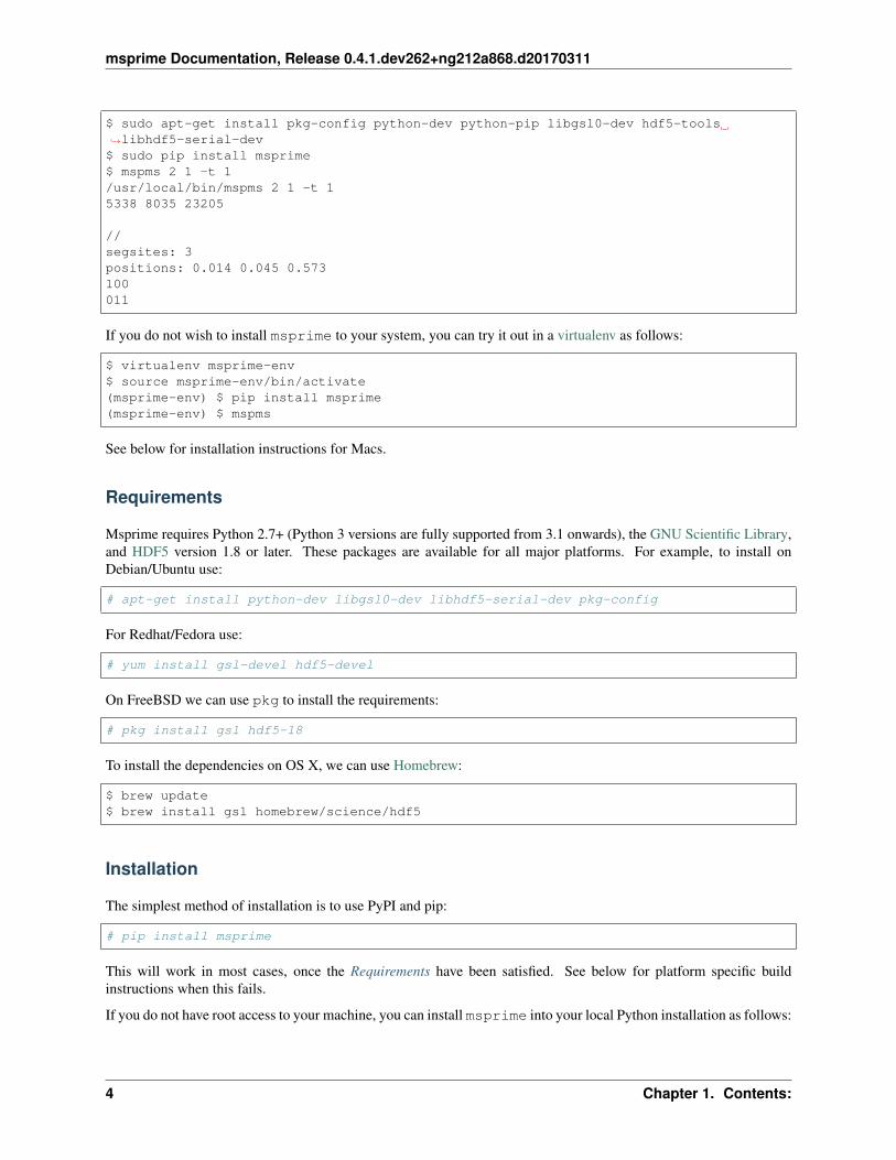
To install and run msprime on a fresh Ubuntu 15.10 installation, do the following:

3

https://www.hdfgroup.org/HDF5/


$ sudo apt-get install pkg-config python-dev python-pip libgsl0-dev hdf5-tools→˓libhdf5-serial-dev$ sudo pip install msprime$ mspms 2 1 -t 1/usr/local/bin/mspms 2 1 -t 15338 8035 23205

//segsites: 3positions: 0.014 0.045 0.573100011

If you do not wish to install msprime to your system, you can try it out in a virtualenv as follows:

$ virtualenv msprime-env$ source msprime-env/bin/activate(msprime-env) $ pip install msprime(msprime-env) $ mspms

See below for installation instructions for Macs.

Requirements

Msprime requires Python 2.7+ (Python 3 versions are fully supported from 3.1 onwards), the GNU Scientific Library,and HDF5 version 1.8 or later. These packages are available for all major platforms. For example, to install onDebian/Ubuntu use:

# apt-get install python-dev libgsl0-dev libhdf5-serial-dev pkg-config

For Redhat/Fedora use:

# yum install gsl-devel hdf5-devel

On FreeBSD we can use pkg to install the requirements:

# pkg install gsl hdf5-18

To install the dependencies on OS X, we can use Homebrew:

$ brew update$ brew install gsl homebrew/science/hdf5

Installation

The simplest method of installation is to use PyPI and pip:

# pip install msprime

This will work in most cases, once the Requirements have been satisfied. See below for platform specific buildinstructions when this fails.

If you do not have root access to your machine, you can install msprime into your local Python installation as follows:

4 Chapter 1. Contents:

http://virtualenv.pypa.io/en/latest/

http://www.gnu.org/software/gsl/


http://brew.sh/


$ pip install msprime --user

To use the mspms program you must ensure that the ~/.local/bin directory is in your PATH, or simply run itusing:

$ ~/.local/bin/mspms

To uninstall msprime, simply run:

$ pip uninstall msprime

Platform specific installation

This section contains instructions to build on platforms that require build time flags for GSL and HDF5.

FreeBSD 10.0

Install the prerequisitites, and build msprime as follows:

# pkg install gsl hdf5-18# CFLAGS=-I/usr/local/include LDFLAGS=-L/usr/local/lib pip install msprime

This assumes that root is logged in using a bash shell. For other shells, different methods are need to set the CFLAGSand LDFLAGS environment variables.

OS X

First, ensure that Homebrew is installed and up-to-date:

$ brew update

We need to ensure that the version of Python we used is installed via Homebrew (there can be issues with linking toHDF5 if we use the built-in version of Python or a version from Anaconda). Therefore, we install Python 3 usinghomebrew:

$ brew install python3$ pip3 install --upgrade pip setuptools

The previous step can be skipped if you wish to use your own Python installation, and already have a working pip.

Now install the dependencies and msprime:

$ brew install gsl homebrew/science/hdf5$ pip3 install msprime

Check if it works:

$ mspms 10 1 -T

1.2. Installation 5


Tutorial

This is the tutorial for the Python interface to the msprime library. Detailed API Documentation is also available forthis library. An ms-compatible command line interface is also available if you wish to use msprime directly withinan existing work flow.

Simulating trees

Running simulations is very straightforward in msprime:

>>> import msprime>>> tree_sequence = msprime.simulate(sample_size=5, Ne=1000)>>> tree = next(tree_sequence.trees())>>> print(tree){0: 5, 1: 7, 2: 5, 3: 7, 4: 6, 5: 6, 6: 8, 7: 8, 8: -1}

Here, we simulate the coalescent for a sample of size 5 with an effective population size of 1000, and then print outa summary of the resulting tree. The simulate() function returns a TreeSequence object, which provides avery efficient way to access the correlated trees in simulations involving recombination. In this example we know thatthere can only be one tree because we have not provided a value for recombination_rate, and it defaults to zero.Therefore, we access the only tree in the sequence using the call next(tree_sequence.trees()).

Trees are represented within msprime in a slightly unusual way. In the majority of libraries dealing with trees, eachnode is represented as an object in memory and the relationship between nodes as pointers between these objects. Inmsprime, however, nodes are integers: the leaves (i.e., our sample) are the integers 0 to 𝑛 − 1, and every internalnode is some positive integer ≥ 𝑛. The result of printing the tree is a summary of how these nodes relate to each otherin terms of their parents. For example, we can see that the parent of nodes 1 and 3 is node 7.

This relationship can be seen more clearly in a picture:

This image shows the same tree as in the example but drawn out in a more familiar format (images like this can bedrawn for any tree using the draw() method). We can see that the leaves of the tree are labelled with 0 to 4, and allthe internal nodes of the tree are also integers with the root of the tree being 8. Also shown here are the times for eachinternal node in generations. (The time for all leaves is 0, and so we don’t show this information to avoid clutter.)

Knowing that our leaves are 0 to 4, we can easily trace our path back to the root for a particular sample using theget_parent() method:

>>> u = 0>>> while u != msprime.NULL_NODE:>>> print("node {}: time = {}".format(u, tree.get_time(u)))>>> u = tree.get_parent(u)node 0: time = 0.0node 5: time = 107.921165302node 6: time = 1006.74711128node 8: time = 1785.36352521

In this code chunk we iterate up the tree starting at node 0 and stop when we get to the root. We know that a nodeis the root if its parent is msprime.NULL_NODE, which is a special reserved node. (The value of the null node is-1, but we recommend using the symbolic constant to make code more readable.) We also use the get_time()method to get the time for each node, which corresponds to the time in generations at which the coalescence eventhappened during the simulation. We can also obtain the length of a branch joining a node to its parent using theget_branch_length() method:



>>> print(tree.get_branch_length(6))778.616413923

The branch length for node 6 is 778.6 generations as the time for node 6 is 1006.7 and the time of its parent is 1785.4.It is also often useful to obtain the total branch length of the tree, i.e., the sum of the lengths of all branches:

>>> print(tree.get_total_branch_length())>>> 5932.15093686

Recombination

Simulating the history of a single locus is a very useful, but we are most often interesting in simulating the historyof our sample across large genomic regions under the influence of recombination. The msprime API is specificallydesigned to make this common requirement both easy and efficient. To model genomic sequences under the influenceof recombination we have two parameters to the simulate() function. The length parameter specifies the lengthof the simulated sequence in bases, and may be a floating point number. If length is not supplied, it is assumed tobe 1. The recombination_rate parameter specifies the rate of crossing over per base per generation, and is zeroby default. See the API Documentation for a discussion of the precise recombination model used.

Here, we simulate the trees across over a 10kb region with a recombination rate of 2× 10−8 per base per generation,with an effective population size of 1000:

>>> tree_sequence = msprime.simulate(... sample_size=5, Ne=1000, length=1e4, recombination_rate=2e-8)>>> for tree in tree_sequence.trees():... print(tree.get_interval(), str(tree), sep="\t")(0.0, 4701.4225005874) {0: 6, 1: 5, 2: 6, 3: 9, 4: 5, 5: 7, 6: 7, 7: 9, 9: -1}(4701.4225005874, 10000.0) {0: 6, 1: 5, 2: 6, 3: 8, 4: 5, 5: 8, 6: 9, 8: 9, 9: -1}

In this example, we use the trees() method to iterate over the trees in the sequence. For each tree we print out theinterval the tree covers (i.e., the genomic coordinates which all share precisely this tree) using the get_interval()method. Thus, the first tree covers the first 4.7kb of sequence and the second tree covers the remaining 5.3kb. Wealso print out the summary of each tree in terms of the parent values for each tree. Again, these differences are bestillustrated by some images:

(We have suppressed the node time labels here for clarity.) We can see that these trees share a great deal of theirstructure, but that there are also important differences between the trees.

Warning: Do not store the values returned from the trees() iterator in a list and operate on them afterwards!For efficiency reasons msprime uses the same instance of SparseTree for each tree in the sequence and updatesthe internal state for each new tree. Therefore, if you store the trees returned from the iterator in a list, they will allrefer to the same tree.

Mutations

Mutations are generated in msprime by throwing mutations down on the branches of trees at a particular rate. Themutations are generated under the infinite sites model, and so each mutation occurs at a unique (floating point) pointposition along the genomic interval occupied by a tree. The mutation rate for simulations is specified using the

1.3. Tutorial 7


mutation_rate parameter of simulate(). For example, to add some mutations to our example above, we canuse:

>>> tree_sequence = msprime.simulate(... sample_size=5, Ne=1000, length=1e4, recombination_rate=2e-8, mutation_rate=2e-→˓8)>>> print("Total mutations = ", tree_sequence.get_num_mutations())>>> for tree in tree_sequence.trees():>>> print(tree.get_interval(), list(tree.mutations()), sep="\t")Total mutations = 1(0.0, 4701.4225005874) [](4701.4225005874, 10000.0) [Mutation(position=5461.212369738915, node=6,→˓index=0)]

In this example (which has the same genealogies as our example above because we use the same random seed), we haveone mutation which falls on the second tree. Mutations are represented as an object with three attributes: positionis the location of the mutation in genomic coordinates, node is the node in the tree above which the mutation occurs,and index is the (zero-based) index of the mutation in the list. Positions are given as a floating point value as we areusing the infinite sites model. Every mutation falls on exactly one tree and we obtain the mutations for a particulartree using the mutations() method. Mutations are always returned in increasing order of position. The mutationin this example is shown as a red box on the corresponding branch:

We can calculate the allele frequency of mutations easily and efficiently using the get_num_leaves() whichreturns the number of leaves underneath a particular node. For example,:

>>> for tree in tree_sequence.trees():... for position, node in tree.mutations():... print("Mutation @ position {} has frequency {}".format(... mutation.position,... tree.get_num_leaves(mutation.node) / tree.get_sample_size()))Mutation @ position 5461.21236974 has frequency 0.4

Sometimes we are only interested in a subset of the mutations in a tree sequence. In these situations, it is useful (andefficient) to update the tree sequence to only include the mutations we are interested in using the TreeSequence.set_mutations() method. Here, for example, we simulate some data and then retain only the common variantswhere the allele frequency is greater than 0.5.

import msprime

def set_mutations_example():tree_sequence = msprime.simulate(

sample_size=10000, Ne=1e4, length=1e7, recombination_rate=2e-8,mutation_rate=2e-8)

print("Simulated ", tree_sequence.get_num_mutations(), "mutations")common_mutations = []for tree in tree_sequence.trees():

for mutation in tree.mutations():p = tree.get_num_leaves(mutation.node) / tree.get_sample_size()if p >= 0.5:

common_mutations.append(mutation)tree_sequence.set_mutations(common_mutations)print("Reduced to ", tree_sequence.get_num_mutations(), "common mutations")

Running this code, we get:



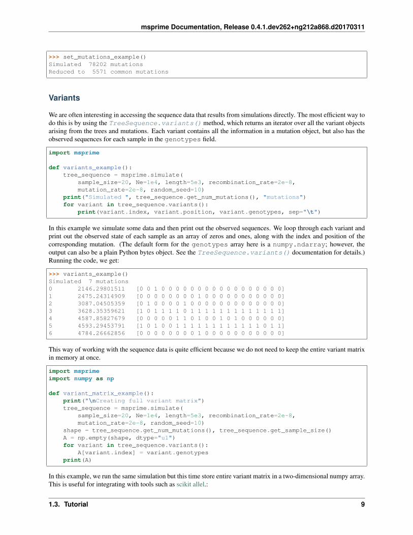
>>> set_mutations_example()Simulated 78202 mutationsReduced to 5571 common mutations

Variants

We are often interesting in accessing the sequence data that results from simulations directly. The most efficient way todo this is by using the TreeSequence.variants() method, which returns an iterator over all the variant objectsarising from the trees and mutations. Each variant contains all the information in a mutation object, but also has theobserved sequences for each sample in the genotypes field.

import msprime

def variants_example():tree_sequence = msprime.simulate(

sample_size=20, Ne=1e4, length=5e3, recombination_rate=2e-8,mutation_rate=2e-8, random_seed=10)

print("Simulated ", tree_sequence.get_num_mutations(), "mutations")for variant in tree_sequence.variants():

print(variant.index, variant.position, variant.genotypes, sep="\t")

In this example we simulate some data and then print out the observed sequences. We loop through each variant andprint out the observed state of each sample as an array of zeros and ones, along with the index and position of thecorresponding mutation. (The default form for the genotypes array here is a numpy.ndarray; however, theoutput can also be a plain Python bytes object. See the TreeSequence.variants() documentation for details.)Running the code, we get:

>>> variants_example()Simulated 7 mutations0 2146.29801511 [0 0 1 0 0 0 0 0 0 0 0 0 0 0 0 0 0 0 0 0]1 2475.24314909 [0 0 0 0 0 0 0 0 1 0 0 0 0 0 0 0 0 0 0 0]2 3087.04505359 [0 1 0 0 0 0 1 0 0 0 0 0 0 0 0 0 0 0 0 0]3 3628.35359621 [1 0 1 1 1 1 0 1 1 1 1 1 1 1 1 1 1 1 1 1]4 4587.85827679 [0 0 0 0 0 1 1 0 1 0 0 1 0 1 0 0 0 0 0 0]5 4593.29453791 [1 0 1 0 0 1 1 1 1 1 1 1 1 1 1 1 1 0 1 1]6 4784.26662856 [0 0 0 0 0 0 0 0 1 0 0 0 0 0 0 0 0 0 0 0]

This way of working with the sequence data is quite efficient because we do not need to keep the entire variant matrixin memory at once.

import msprimeimport numpy as np

def variant_matrix_example():print("\nCreating full variant matrix")tree_sequence = msprime.simulate(

sample_size=20, Ne=1e4, length=5e3, recombination_rate=2e-8,mutation_rate=2e-8, random_seed=10)

shape = tree_sequence.get_num_mutations(), tree_sequence.get_sample_size()A = np.empty(shape, dtype="u1")for variant in tree_sequence.variants():

A[variant.index] = variant.genotypesprint(A)

In this example, we run the same simulation but this time store entire variant matrix in a two-dimensional numpy array.This is useful for integrating with tools such as scikit allel.:

1.3. Tutorial 9

https://scikit-allel.readthedocs.io/en/latest/


>>> variant_matrix_example()Creating full variant matrix[[0 0 1 0 0 0 0 0 0 0 0 0 0 0 0 0 0 0 0 0][0 0 0 0 0 0 0 0 1 0 0 0 0 0 0 0 0 0 0 0][0 1 0 0 0 0 1 0 0 0 0 0 0 0 0 0 0 0 0 0][1 0 1 1 1 1 0 1 1 1 1 1 1 1 1 1 1 1 1 1][0 0 0 0 0 1 1 0 1 0 0 1 0 1 0 0 0 0 0 0][1 0 1 0 0 1 1 1 1 1 1 1 1 1 1 1 1 0 1 1][0 0 0 0 0 0 0 0 1 0 0 0 0 0 0 0 0 0 0 0]]

Historical samples

Simulating coalescent histories in which some of the samples are not from the present time is straightforward inmsprime. By using the samples argument to msprime.simulate() we can specify the location and time atwhich all samples are made.

def historical_samples_example():samples = [

msprime.Sample(population=0, time=0),msprime.Sample(0, 0), # Or, we can use positional arguments.msprime.Sample(0, 1.0)

]tree_seq = msprime.simulate(samples=samples)tree = next(tree_seq.trees())for u in range(tree_seq.get_num_nodes()):

print(u, tree.get_parent(u), tree.get_time(u), sep="\t")

In this example we create three samples, two taken at the present time and one taken 1.0 generations in the past. Thereare a number of different ways in which we can describe the samples using the msprime.Sample object (samplescan be provided as plain tuples also if more convenient). Running this example, we get:

>>> historical_samples_example()0 3 0.01 3 0.02 4 1.03 4 0.5020399553844 -1 4.5595966593

Because nodes 0 and 1 were sampled at time 0, their times in the tree are both 0. Node 2 was sampled at time 1.0,and so its time is recorded as 1.0 in the tree.

Replication

A common task for coalescent simulations is to check the accuracy of analytical approximations to statistics of interest.To do this, we require many independent replicates of a given simulation. msprime provides a simple and efficientAPI for replication: by providing the num_replicates argument to the simulate() function, we can iterateover the replicates in a straightforward manner. Here is an example where we compare the analytical results for thenumber of segregating sites with simulations:


def segregating_sites_example(n, theta, num_replicates):S = np.zeros(num_replicates)



replicates = msprime.simulate(sample_size=n,mutation_rate=theta / 4,num_replicates=num_replicates)

for j, tree_sequence in enumerate(replicates):S[j] = tree_sequence.get_num_mutations()

# Now, calculate the analytical predictionsS_mean_a = np.sum(1 / np.arange(1, n)) * thetaS_var_a = (

theta * np.sum(1 / np.arange(1, n)) +theta**2 * np.sum(1 / np.arange(1, n)**2))

print(" mean variance")print("Observed {}\t\t{}".format(np.mean(S), np.var(S)))print("Analytical {:.5f}\t\t{:.5f}".format(S_mean_a, S_var_a))

Running this code, we get:

>>> segregating_sites_example(10, 5, 100000)mean variance

Observed 14.12173 52.4695318071Analytical 14.14484 52.63903

Note that in this example we did not provide a value for the Ne argument to simulate(). In this case the effectivepopulation size defaults to 1, which can be useful for theoretical work. However, it is essential to remember that allrates and times must still be scaled by 4 to convert into the coalescent time scale.

Population structure

Population structure in msprime closely follows the model used in the ms simulator: we have 𝑁 demes with an𝑁 × 𝑁 matrix describing the migration rates between these subpopulations. The sample sizes, population sizes andgrowth rates of all demes can be specified independently. Migration rates are specified using a migration matrix.Unlike ms however, all times and rates are specified in generations and all populations sizes are absolute (that is, notmultiples of 𝑁𝑒).

In the following example, we calculate the mean coalescence time for a pair of lineages sampled in different demes ina symmetric island model, and compare this with the analytical expectation.


def migration_example():# M is the overall symmetric migration rate, and d is the number# of demes.M = 0.2d = 3# We rescale m into per-generation values for msprime.m = M / (4 * (d - 1))# Allocate the initial sample. Because we are interested in the# between deme coalescence times, we choose one sample each# from the first two demes.population_configurations = [

msprime.PopulationConfiguration(sample_size=1),msprime.PopulationConfiguration(sample_size=1),msprime.PopulationConfiguration(sample_size=0)]

# Now we set up the migration matrix. Since this is a symmetric# island model, we have the same rate of migration between all

1.3. Tutorial 11


# pairs of demes. Diagonal elements must be zero.migration_matrix = [

[0, m, m],[m, 0, m],[m, m, 0]]

# We pass these values to the simulate function, and ask it# to run the required number of replicates.num_replicates = 1e6replicates = msprime.simulate(

population_configurations=population_configurations,migration_matrix=migration_matrix,num_replicates=num_replicates)

# And then iterate over these replicatesT = np.zeros(num_replicates)for i, tree_sequence in enumerate(replicates):

tree = next(tree_sequence.trees())# Convert the TMRCA to coalecent units.T[i] = tree.get_time(tree.get_root()) / 4

# Finally, calculate the analytical expectation and print# out the resultsanalytical = d / 2 + (d - 1) / (2 * M)print("Observed =", np.mean(T))print("Predicted =", analytical)

Running this example we get:

>>> migration_example()Observed = 6.50638181614Predicted = 6.5

Demography

Msprime provides a flexible and simple way to model past demographic events in arbitrary combinations. Here is anexample describing the Gutenkunst et al. out-of-Africa model. See Figure 2B for a schematic of this model, and Table1 for the values used.

Todo

Add a diagram of the model for convenience.

def out_of_africa():# First we set out the maximum likelihood values of the various parameters# given in Table 1.N_A = 7300N_B = 2100N_AF = 12300N_EU0 = 1000N_AS0 = 510# Times are provided in years, so we convert into generations.generation_time = 25T_AF = 220e3 / generation_timeT_B = 140e3 / generation_timeT_EU_AS = 21.2e3 / generation_time# We need to work out the starting (diploid) population sizes based on# the growth rates provided for these two populations


http://dx.doi.org/10.1371/journal.pgen.1000695

http://dx.doi.org/10.1371/journal.pgen.1000695.g002

http://dx.doi.org/10.1371/journal.pgen.1000695.t001

http://dx.doi.org/10.1371/journal.pgen.1000695.t001


r_EU = 0.004r_AS = 0.0055N_EU = N_EU0 / math.exp(-r_EU * T_EU_AS)N_AS = N_AS0 / math.exp(-r_AS * T_EU_AS)# Migration rates during the various epochs.m_AF_B = 25e-5m_AF_EU = 3e-5m_AF_AS = 1.9e-5m_EU_AS = 9.6e-5# Population IDs correspond to their indexes in the population# configuration array. Therefore, we have 0=YRI, 1=CEU and 2=CHB# initially.population_configurations = [

msprime.PopulationConfiguration(sample_size=0, initial_size=N_AF),

msprime.PopulationConfiguration(sample_size=1, initial_size=N_EU, growth_rate=r_EU),

msprime.PopulationConfiguration(sample_size=1, initial_size=N_AS, growth_rate=r_AS)

]migration_matrix = [

[ 0, m_AF_EU, m_AF_AS],[m_AF_EU, 0, m_EU_AS],[m_AF_AS, m_EU_AS, 0],

]demographic_events = [

# CEU and CHB merge into B with rate changes at T_EU_ASmsprime.MassMigration(

time=T_EU_AS, source=2, destination=1, proportion=1.0),msprime.MigrationRateChange(time=T_EU_AS, rate=0),msprime.MigrationRateChange(

time=T_EU_AS, rate=m_AF_B, matrix_index=(0, 1)),msprime.MigrationRateChange(

time=T_EU_AS, rate=m_AF_B, matrix_index=(1, 0)),msprime.PopulationParametersChange(

time=T_EU_AS, initial_size=N_B, growth_rate=0, population_id=1),# Population B merges into YRI at T_Bmsprime.MassMigration(

time=T_B, source=1, destination=0, proportion=1.0),# Size changes to N_A at T_AFmsprime.PopulationParametersChange(

time=T_AF, initial_size=N_A, population_id=0)]# Use the demography debugger to print out the demographic history# that we have just described.dp = msprime.DemographyDebugger(

Ne=N_A,population_configurations=population_configurations,migration_matrix=migration_matrix,demographic_events=demographic_events)

dp.print_history()

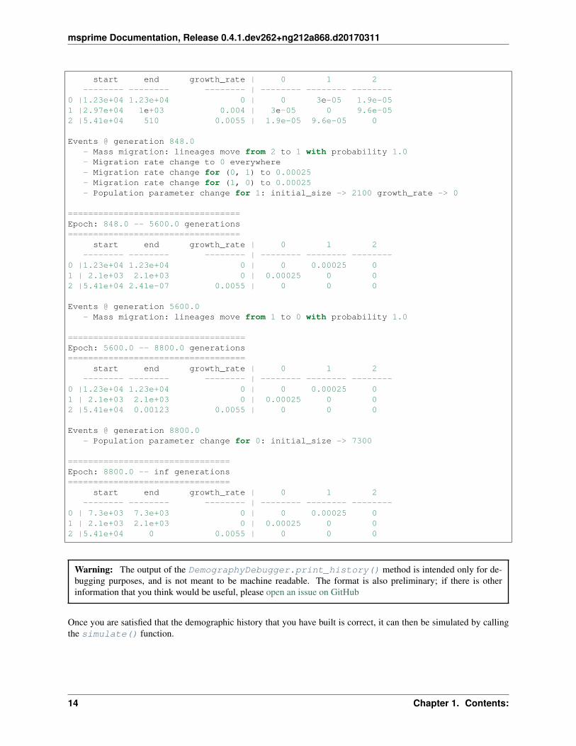
The DemographyDebugger provides a method to debug the history that you have described so that you can be surethat the migration rates, population sizes and growth rates are all as you intend during each epoch:

=============================Epoch: 0 -- 848.0 generations=============================

1.3. Tutorial 13


start end growth_rate | 0 1 2-------- -------- -------- | -------- -------- --------

0 |1.23e+04 1.23e+04 0 | 0 3e-05 1.9e-051 |2.97e+04 1e+03 0.004 | 3e-05 0 9.6e-052 |5.41e+04 510 0.0055 | 1.9e-05 9.6e-05 0

Events @ generation 848.0- Mass migration: lineages move from 2 to 1 with probability 1.0- Migration rate change to 0 everywhere- Migration rate change for (0, 1) to 0.00025- Migration rate change for (1, 0) to 0.00025- Population parameter change for 1: initial_size -> 2100 growth_rate -> 0

==================================Epoch: 848.0 -- 5600.0 generations==================================


0 |1.23e+04 1.23e+04 0 | 0 0.00025 01 | 2.1e+03 2.1e+03 0 | 0.00025 0 02 |5.41e+04 2.41e-07 0.0055 | 0 0 0

Events @ generation 5600.0- Mass migration: lineages move from 1 to 0 with probability 1.0

===================================Epoch: 5600.0 -- 8800.0 generations===================================


0 |1.23e+04 1.23e+04 0 | 0 0.00025 01 | 2.1e+03 2.1e+03 0 | 0.00025 0 02 |5.41e+04 0.00123 0.0055 | 0 0 0

Events @ generation 8800.0- Population parameter change for 0: initial_size -> 7300

================================Epoch: 8800.0 -- inf generations================================


0 | 7.3e+03 7.3e+03 0 | 0 0.00025 01 | 2.1e+03 2.1e+03 0 | 0.00025 0 02 |5.41e+04 0 0.0055 | 0 0 0

Warning: The output of the DemographyDebugger.print_history() method is intended only for de-bugging purposes, and is not meant to be machine readable. The format is also preliminary; if there is otherinformation that you think would be useful, please open an issue on GitHub

Once you are satisfied that the demographic history that you have built is correct, it can then be simulated by callingthe simulate() function.


https://github.com/jeromekelleher/msprime/issues


Recombination maps

The msprimeAPI allows us to quickly and easily simulate data from an arbitrary recombination map. In this examplewe read a recombination map for human chromosome 22, and simulate a single replicate. After the simulation iscompleted, we plot histograms of the recombination rates and the simulated breakpoints. These show that density ofbreakpoints follows the recombination rate closely.

import numpy as npimport scipy.statsimport matplotlib.pyplot as pyplot

def variable_recomb_example():infile = "hapmap/genetic_map_GRCh37_chr22.txt"# Read in the recombination map using the read_hapmap method,recomb_map = msprime.RecombinationMap.read_hapmap(infile)

# Now we get the positions and rates from the recombination# map and plot these using 500 bins.positions = np.array(recomb_map.get_positions()[1:])rates = np.array(recomb_map.get_rates()[1:])num_bins = 500v, bin_edges, _ = scipy.stats.binned_statistic(

positions, rates, bins=num_bins)x = bin_edges[:-1][np.logical_not(np.isnan(v))]y = v[np.logical_not(np.isnan(v))]fig, ax1 = pyplot.subplots(figsize=(16, 6))ax1.plot(x, y, color="blue")ax1.set_ylabel("Recombination rate")ax1.set_xlabel("Chromosome position")

# Now we run the simulation for this map. We assume Ne=10^4# and have a sample of 100 individualstree_sequence = msprime.simulate(

sample_size=100,Ne=10**4,recombination_map=recomb_map)

# Now plot the density of breakpoints along the chromosomebreakpoints = np.array(list(tree_sequence.breakpoints()))ax2 = ax1.twinx()v, bin_edges = np.histogram(breakpoints, num_bins, density=True)ax2.plot(bin_edges[:-1], v, color="green")ax2.set_ylabel("Breakpoint density")ax2.set_xlim(1.5e7, 5.3e7)fig.savefig("hapmap_chr22.svg")

Calculating LD

The msprime API provides methods to efficiently calculate population genetics statistics. For example, theLdCalculator class allows us to compute pairwise linkage disequilibrium coefficients. Here we use theget_r2_matrix() method to easily make an LD plot using matplotlib. (Thanks to the excellent scikit-allel for thebasic plotting code used here.)

import msprimeimport matplotlib.pyplot as pyplot

1.3. Tutorial 15

https://en.wikipedia.org/wiki/Linkage_disequilibrium

http://matplotlib.org/

http://scikit-allel.readthedocs.io/en/latest/index.html

http://scikit-allel.readthedocs.io/en/latest/_modules/allel/stats/ld.html#plot_pairwise_ld


def ld_matrix_example():ts = msprime.simulate(100, recombination_rate=10, mutation_rate=20,

random_seed=1)ld_calc = msprime.LdCalculator(ts)A = ld_calc.get_r2_matrix()# Now plot this matrix.x = A.shape[0] / pyplot.rcParams['savefig.dpi']x = max(x, pyplot.rcParams['figure.figsize'][0])fig, ax = pyplot.subplots(figsize=(x, x))fig.tight_layout(pad=0)im = ax.imshow(A, interpolation="none", vmin=0, vmax=1, cmap="Blues")ax.set_xticks([])ax.set_yticks([])for s in 'top', 'bottom', 'left', 'right':

ax.spines[s].set_visible(False)pyplot.gcf().colorbar(im, shrink=.5, pad=0)pyplot.savefig("ld.svg")

Working with threads

When performing large calculations it’s often useful to split the work over multiple processes or threads. The msprimeAPI can be used without issues across multiple processes, and the Python multiprocessing module often pro-vides a very effective way to work with many replicate simulations in parallel.

When we wish to work with a single very large dataset, however, threads can offer better resource usage because ofthe shared memory space. The Python threading library gives a very simple interface to lightweight CPU threadsand allows us to perform several CPU intensive tasks in parallel. The msprime API is designed to allow multiplethreads to work in parallel when CPU intensive tasks are being undertaken.

Note: In the CPython implementation the Global Interpreter Lock ensures that only one thread executes Pythonbytecode at one time. This means that Python code does not parallelise well across threads, but avoids a large numberof nasty pitfalls associated with multiple threads updating data structures in parallel. Native C extensions like numpyand msprime release the GIL while expensive tasks are being performed, therefore allowing these calculations toproceed in parallel.

In the following example we wish to find all mutations that are in approximate LD (𝑟2 ≥ 0.5) with a given set ofmutations. We parallelise this by splitting the input array between a number of threads, and use the LdCalculator.get_r2_array() method to compute the 𝑟2 value both up and downstream of each focal mutation, filter out thosethat exceed our threshold, and store the results in a dictionary. We also use the very cool tqdm module to give us aprogress bar on this computation.

import threadingimport numpy as npimport tqdmimport msprime

def find_ld_sites(tree_sequence, focal_mutations, max_distance=1e6, r2_threshold=0.5,num_threads=8):

results = {}progress_bar = tqdm.tqdm(total=len(focal_mutations))num_threads = min(num_threads, len(focal_mutations))


https://docs.python.org/2/library/multiprocessing.html#module-multiprocessing

https://docs.python.org/2/library/threading.html#module-threading

https://wiki.python.org/moin/GlobalInterpreterLock

https://pypi.python.org/pypi/tqdm


def thread_worker(thread_index):ld_calc = msprime.LdCalculator(tree_sequence)chunk_size = int(math.ceil(len(focal_mutations) / num_threads))start = thread_index * chunk_sizefor focal_mutation in focal_mutations[start: start + chunk_size]:

a = ld_calc.get_r2_array(focal_mutation, max_distance=max_distance,direction=msprime.REVERSE)

rev_indexes = focal_mutation - np.nonzero(a >= r2_threshold)[0] - 1a = ld_calc.get_r2_array(

focal_mutation, max_distance=max_distance,direction=msprime.FORWARD)

fwd_indexes = focal_mutation + np.nonzero(a >= r2_threshold)[0] + 1indexes = np.concatenate((rev_indexes[::-1], fwd_indexes))results[focal_mutation] = indexesprogress_bar.update()

threads = [threading.Thread(target=thread_worker, args=(j,))for j in range(num_threads)]

for t in threads:t.start()

for t in threads:t.join()

progress_bar.close()return results

def threads_example():ts = msprime.simulate(

sample_size=1000, Ne=1e4, length=1e7, recombination_rate=2e-8,mutation_rate=2e-8)

counts = np.zeros(ts.get_num_mutations())for t in ts.trees():

for mutation in t.mutations():counts[mutation.index] = t.get_num_leaves(mutation.node)

doubletons = np.nonzero(counts == 2)[0]results = find_ld_sites(ts, doubletons, num_threads=8)print(

"Found LD sites for", len(results), "doubleton mutations out of",ts.get_num_mutations())

In this example, we first simulate 1000 samples of 10 megabases and find all doubleton mutations in the resulting treesequence. We then call the find_ld_sites() function to find all mutations that are within 1 megabase of thesedoubletons and have an 𝑟2 statistic of greater than 0.5.

The find_ld_sites() function performs these calculations in parallel using 8 threads. The real work is donein the nested thread_worker() function, which is called once by each thread. In the thread worker, we firstallocate an instance of the LdCalculator class. (It is critically important that each thread has its own instanceof LdCalculator, as the threads will not work efficiently otherwise.) After this, each thread works out the slice ofthe input array that it is responsible for, and then iterates over each focal mutation in turn. After the 𝑟2 values havebeen calculated, we then find the indexes of the mutations corresponding to values greater than 0.5 using numpy.nonzero(). Finally, the thread stores the resulting array of mutation indexes in the results dictionary, andmoves on to the next focal mutation.

Running this example we get:

1.3. Tutorial 17


>>> threads_example()100%|| 4045/4045 [00:09<00:00, 440.29it/s]Found LD sites for 4045 doubleton mutations out of 60100

API Documentation

This is the API documentation for msprime, and provides detailed information on the Python programming interface.See the Tutorial for an introduction to using this API to run simulations and analyse the results.

Simulation model

The simulation model in msprime closely follows the classical ms program. Unlike ms, however, time is measured ingenerations rather than “coalescent units”. Internally the same simulation algorithm is used, but msprime providesa translation layer to allow the user input times and rates in generations. Similarly, the times associated with thetrees produced by msprime are in measured generations. To enable this translation from generations into coalescentunits and vice-versa, a reference effective population size must be provided, which is given by the Ne parameterin the simulate() function. (Note that we assume diploid population sizes thoughout, since we scale by 4𝑁𝑒.)Population sizes for individual demes and for past demographic events are defined as absolute values, not scaled byNe. All migration rates and growth rates are also per generation.

When running simulations we define the length in bases 𝐿 of the sequence in question using the length parameter.This defines the coordinate space within which trees and mutations are defined. 𝐿 is a continuous value, and coordi-nates can take any value from 0 to 𝐿. Mutations occur in an infinite sites process along this sequence, and mutationrates are specified per generation, per unit of sequence length. Thus, given the per-generation mutation rate 𝜇, the rateof mutation over the entire sequence in coalescent time units is 𝜃 = 4𝑁𝑒𝜇𝐿. It is important to remember these scalingfactors when comparing with analytical results!

Similarly, recombination rates are per base, per generation in msprime. Thus, given the per generation crossoverrate 𝑟, the overall rate of recombination between the ends of the sequence in coalescent time units is 𝜌 = 4𝑁𝑒𝑟𝐿.Recombination events occur in a continuous coordinate space, so that breakpoints do not necessarily occur at integerlocations. However, the underlying recombination model is finite, and the behaviour of a small number of loci can bemodelled using the RecombinationMap class. However, this is considered an advanced feature and the majorityof cases should be well served with the default recombination model and number of loci.

Population structure is modelled by specifying a fixed number of demes 𝑑, and a 𝑑 × 𝑑 matrix 𝑀 of per generationmigration rates. Each element of the matrix 𝑀𝑗,𝑘 defines the fraction of population 𝑗 that consists of migrants frompopulation 𝑘 in each generation. Each deme has an initial absolute population size 𝑠 and a per generation exponentialgrowth rate 𝛼. The size of a given population at time 𝑡 in the past (measured in generations) is therefore given by𝑠𝑒−𝛼𝑡. Demographic events that occur in the history of the simulated population alter some aspect of this populationconfiguration at a particular time in the past.

Warning: This parameterisation of recombination, mutation and migration rates is different to ms, which statesthese rates over the entire region and in coalescent time units. The motivation for this is to allow the user changethe size of the simulated region without having to rescale the recombination and mutation rates, and to also allowusers directly state times and rates in units of generations. However, the mspms command line application is fullyms compatible.

Running simulations

The simulate() function provides the primary interface to running coalescent simulations in msprime.



msprime.simulate(sample_size=None, Ne=1, length=None, recombination_rate=None, recombi-nation_map=None, mutation_rate=None, population_configurations=None, mi-gration_matrix=None, demographic_events=[], samples=None, model=None,record_migrations=False, random_seed=None, mutation_generator=None,num_replicates=None)

Simulates the coalescent with recombination under the specified model parameters and returns the resultingTreeSequence.

Parameters

• sample_size (int) – The number of individuals in our sample. If not specified orNone, this defaults to the sum of the subpopulation sample sizes. Either sample_size,population_configurations or samples must be specified.

• Ne (float) – The effective (diploid) population size for the reference population. Thisdetermines the factor by which the per-generation recombination and mutation rates arescaled in the simulation. This defaults to 1 if not specified.

• length (float) – The length of the simulated region in bases. This parameter cannot beused along with recombination_map. Defaults to 1 if not specified.

• recombination_rate (float) – The rate of recombination per base per generation.This parameter cannot be used along with recombination_map. Defaults to 0 if notspecified.

• recombination_map (RecombinationMap) – The map describing the changingrates of recombination along the simulated chromosome. This parameter cannot beused along with the recombination_rate or length parameters, as these val-ues are encoded within the map. Defaults to a uniform rate as described in therecombination_rate parameter if not specified.

• mutation_rate (float) – The rate of mutation per base per generation. If not speci-fied, no mutations are generated.

• population_configurations (list or None.) – The list ofPopulationConfiguration instances describing the sampling configuration,relative sizes and growth rates of the populations to be simulated. If this is not specified, asingle population with a sample of size sample_size is assumed.

• migration_matrix (list) – The matrix describing the rates of migra-tion between all pairs of populations. If 𝑁 populations are defined in thepopulation_configurations parameter, then the migration matrix must bean 𝑁 ×𝑁 matrix consisting of 𝑁 lists of length 𝑁 .

• demographic_events (list) – The list of demographic events to simulate. Demo-graphic events describe changes to the populations in the past. Events should be supplied innon-decreasing order of time. Events with the same time value will be applied sequentiallyin the order that they were supplied before the simulation algorithm continues with the nexttime step.

• samples (list) – The list specifying the location and time of all samples. This param-eter may be used to specify historical samples, and cannot be used in conjunction with thesample_size parameter. Each sample is a (population_id, time) pair such that thesample in position j in the list of samples is drawn in the specified population at the specfiedtime. Time is measured in generations, as elsewhere.

• random_seed (int) – The random seed. If this is None, a random seed will be automat-ically generated. Valid random seeds must be between 1 and 232 − 1.

• num_replicates (int) – The number of replicates of the specified parameters to sim-ulate. If this is not specified or None, no replication is performed and a TreeSequence

1.4. API Documentation 19

https://docs.python.org/2/library/functions.html#int

https://docs.python.org/2/library/functions.html#float




https://docs.python.org/2/library/functions.html#list







object returned. If num_replicates is provided, the specified number of replicates isperformed, and an iterator over the resulting TreeSequence objects returned.

Returns The TreeSequence object representing the results of the simulation if no replication isperformed, or an iterator over the independent replicates simulated if the num_replicatesparameter has been used.

Return type TreeSequence or an iterator over TreeSequence replicates.

Warning If using replication, do not store the results of the iterator in a list! For performancereasons, the same underlying object may be used for every TreeSequence returned which willmost likely lead to unexpected behaviour.

Population structure

Population structure is modelled in msprime by specifying a fixed number of demes, with the migration rates betweenthose demes defined by a migration matrix. Each deme has an initial_size that defines its absolute size attime zero and a per-generation growth_rate which specifies the exponential growth rate of the sub-population.We must also define the size of the sample to draw from each deme. The number of populations and their initialconfiguration is defined using the population_configurations parameter to simulate(), which takes alist of PopulationConfiguration instances. Population IDs are zero indexed, and correspond to their positionin the list.

Samples are drawn sequentially from populations in increasing order of population ID. For example, if we specifiedan overall sample size of 5, and specify that 2 samples are drawn from population 0 and 3 from population 1, thenindividuals 0 and 1 will be initially located in population 0, and individuals 2, 3 and 4 will be drawn from population2.

Given 𝑁 populations, migration matrices are specified using an 𝑁 ×𝑁 matrix of deme-to-deme migration rates. Seethe documentation for simulate() and the Simulation model section for more details on the migration rates.

class msprime.PopulationConfiguration(sample_size=None, initial_size=None,growth_rate=0.0)

The initial configuration of a population (or deme) in a simulation.

Parameters

• sample_size (int) – The number of initial samples that are drawn from this population.

• initial_size (float) – The absolute size of the population at time zero. Defaults tothe reference population size 𝑁𝑒.

• growth_rate (float) – The exponential growth rate of the population per generation.Growth rates can be negative. This is zero for a constant population size. Defaults to 0.

Demographic Events

Demographic events change some aspect of the population configuration at some time in the past, and are specifiedusing the demographic_events parameter to simulate(). Each element of this list must be an instance of oneof the following demographic events that are currently supported. Note that all times are measured in generations, allsizes are absolute (i.e., not relative to 𝑁𝑒), and all rates are per-generation.

class msprime.PopulationParametersChange(time, initial_size=None, growth_rate=None, popula-tion_id=None)

Changes the demographic parameters of a population at a given time.

This event generalises the -eg, -eG, -en and -eN options from ms. Note that unlike ms we do not automati-cally set growth rates to zero when the population size is changed.






Parameters

• time (float) – The time at which this event occurs in generations.

• initial_size (float) – The absolute size of the population at the beginning of thetime slice starting at time. If None, this is calculated according to the initial populationsize and growth rate over the preceding time slice.

• growth_rate (float) – The new per-generation growth rate. If None, the growth rateis not changed. Defaults to None.

• population_id (int) – The ID of the population affected. If population_id isNone, the changes affect all populations simultaneously.

class msprime.MigrationRateChange(time, rate, matrix_index=None)Changes the rate of migration to a new value at a specific time.

Parameters


• rate (float) – The new per-generation migration rate.

• matrix_index (tuple) – A tuple of two population IDs descibing the matrix index ofinterest. If matrix_index is None, all non-diagonal entries of the migration matrix arechanged simultaneously.

class msprime.MassMigration(time, source, destination, proportion=1.0)A mass migration event in which some fraction of the population in one deme simultaneously move to anotherdeme, viewed backwards in time. For each lineage currently present in the source population, they move to thedestination population with probability equal to proportion.

This event class generalises the population split (-ej) and admixture (-es) events from ms. Note that Mass-Migrations do not have any side effects on the migration matrix.

Parameters


• source (int) – The ID of the source population.

• destination (int) – The ID of the destination population.

• proportion (float) – The probability that any given lineage within the source popula-tion migrates to the destination population.

Debugging demographic models

Warning: The DemographyDebugger class is preliminary, and the API is likely to change in the future.

class msprime.DemographyDebugger(Ne=1, population_configurations=None, migra-tion_matrix=None, demographic_events=[])

A class to facilitate debugging of population parameters and migration rates in the past.

print_history(output=<open file ‘<stdout>’, mode ‘w’>)Prints a summary of the history of the populations.








https://docs.python.org/2/library/functions.html#tuple






Variable recombination rates

class msprime.RecombinationMap(positions, rates, num_loci=None)A RecombinationMap represents the changing rates of recombination along a chromosome. This is defined viatwo lists of numbers: positions and rates, which must be of the same length. Given an index j in theselists, the rate of recombination per base per generation is rates[j] over the interval positions[j] topositions[j + 1]. Consequently, the first position must be zero, and by convention the last rate value isalso required to be zero (although it does not used).

Parameters

• positions (list) – The positions (in bases) denoting the distinct intervals where re-combination rates change. These can be floating point values.

• rates (list) – The list of rates corresponding to the supplied positions. Recombi-nation rates are specified per base, per generation.

• num_loci (int) – The maximum number of non-recombining loci in the underlying sim-ulation. By default this is set to the largest possible value, allowing the maximum resolutionin the recombination process. However, for a finite sites model this can be set to smallervalues.

classmethod read_hapmap(filename)Parses the specified file in HapMap format. These files must contain a single header line (which is ig-nored), and then each subsequent line denotes a position/rate pair. Positions are in units of bases, andrecombination rates in centimorgans/Megabase. The first column in this file is ignored, as are subsequencecolumns after the Position and Rate. A sample of this format is as follows:

Chromosome Position(bp) Rate(cM/Mb) Map(cM)chr1 55550 2.981822 0.000000chr1 82571 2.082414 0.080572chr1 88169 2.081358 0.092229chr1 254996 3.354927 0.439456chr1 564598 2.887498 1.478148

Parameters filename (str) – The name of the file to be parsed. This may be in plain text orgzipped plain text.

Processing results

The TreeSequence class represents a sequence of correlated trees output by a simulation. The SparseTree classrepresents a single tree in this sequence.

msprime.NULL_NODE = -1Special reserved value, representing the null node. If the parent of a given node is null, then this node is a root.Similarly, if the children of a node are null, this node is a leaf.

msprime.NULL_POPULATION = -1Special reserved value, representing the null population ID. If the population associated with a particular treenode is not defined, or population information was not available in the underlying tree sequence, then this valuewill be returned by SparseTree.get_population().

msprime.FORWARD = 1Constant representing the forward direction of travel (i.e., increasing coordinate values).

msprime.REVERSE = -1Constant representing the reverse direction of travel (i.e., decreasing coordinate values).





https://docs.python.org/2/library/functions.html#str


msprime.load(path)Loads a tree sequence from the specified file path. This file must be in the HDF5 file format produced by theTreeSequence.dump() method.

Parameters path (str) – The file path of the HDF5 file containing the tree sequence we wish toload.

Returns The tree sequence object containing the information stored in the specified file path.

Return type msprime.TreeSequence

msprime.load_txt(records_file, mutations_file=None)Loads a tree sequence from the specified file paths. The files input here are in a simple whitespace delim-ited tabular format such as output by the TreeSequence.write_records() and TreeSequence.write_mutations() methods. This method is intended as a convenient interface for importing externaldata into msprime; the HDF5 based file format using by msprime.load() will be many times more efficientthat using the text based formats.

The records_file must be a text file with six whitespace delimited columns. Each line in the file mustcontain at least this many columns, and each line will be stored as a single coalescence record. The columnscorrespond to the left, right, node, children, time and population fields as described in theTreeSequence.records() method. The left, right and time fields are parsed as base 10 floatingpoint values, and the node and population fields are parsed as base 10 integers. The children field is acomma-separated list of base 10 integer values, and must contain at least two elements. The file may optionallybegin with a header line; if the first line begins with the text “left” it will be ignored.

Records must be listed in the file in non-decreasing order of the time field. Within a record, children must belisted in increasing order of node value. The left and right coordinates must be non-negative values.

An example of a simple tree sequence for four samples with three distinct trees is:

left right node children time population2 10 4 2,3 0.071 00 2 5 1,3 0.090 02 10 5 1,4 0.090 00 7 6 0,5 0.170 07 10 7 0,5 0.202 00 2 8 2,6 0.253 0

This example is equivalent to the tree sequence illustrated in Figure 4 of the PLoS Computational Biology paper.Nodes are given here in time order (since this is a backwards-in-time tree sequence), but they may be allocatedin any order. In particular, left-to-right tree sequences are fully supported. However, the smallest value in thenode column must be equal to the sample size, and there must not be ‘gaps’ in the node address space.

The optional mutations_file has a similiar format, but contains only two columns. These correspond to theposition and node fields as described in the TreeSequence.mutations() method. The positionfield is parsed as a base 10 floating point value, and the node field is parsed as a base 10 integer. The file mayoptionally begin with a header line; if the first line begins with the text “position” it will be ignored.

Mutations must be listed in non-decreasing order of position, and the nodes must refer to a node defined by therecords. Mutations defined over the root or a node not present in a local tree will lead to an error being producedduring tree traversal (e.g. in the TreeSequence.trees() method, but also in many other methods).

An example of a mutations file for the tree sequence defined in the previous example is:

position node0.1 08.5 4

Parameters



http://dx.doi.org/10.1371/journal.pcbi.1004842


• records_file (str) – The path of the text file containing the coalescence records forthe desired tree sequence.

• mutations_file (str) – The path of the text file containing the mutation records forthe desired tree sequence. This argument is optional and defaults to None.

Returns The tree sequence object containing the information stored in the specified file paths.

Return type msprime.TreeSequence

class msprime.TreeSequenceA TreeSequence represents the information generated in a coalescent simulation. This includes all the treesacross the simulated region, along with the mutations (if any are present).

branch_stats(leaf_sets, weight_fun)Here leaf_sets is a list of lists of leaves, and weight_fun is a function whose argument is a list of integers ofthe same length as leaf_sets that returns a boolean. A branch in a tree is weighted by weight_fun(x), wherex[i] is the number of leaves in leaf_sets[i] below that branch. This finds the sum of all counted branchesfor each tree, and averages this across the tree sequence, weighted by genomic length.

branch_stats_vector(leaf_sets, weight_fun)Here leaf_sets is a list of lists of leaves, and weight_fun is a function whose argument is a list of integers ofthe same length as leaf_sets that returns a boolean. A branch in a tree is weighted by weight_fun(x), wherex[i] is the number of leaves in leaf_sets[i] below that branch. This finds the sum of all counted branchesfor each tree, and averages this across the tree sequence, weighted by genomic length.

breakpoints()Returns an iterator over the breakpoints along the chromosome, including the two extreme points 0 and L.This is equivalent to

>>> [0] + [t.get_interval()[1] for t in self.trees()]

although we do not build an explicit list.

Returns An iterator over all the breakpoints along the simulated sequence.

Return type iter

diffs()Returns an iterator over the differences between adjacent trees in this tree sequence. Each diff returned bythis method is a tuple of the form (length, records_out, records_in). The length is the length of the genomicinterval covered by the current tree, and is equivalent to the value returned by msprime.SparseTree.get_length(). The records_out value is list of (𝑢, 𝑐, 𝑡) tuples, and corresponds to the coalescencerecords that have been invalidated by moving to the current tree. As in the records() method, 𝑢 isa tree node, 𝑐 is a tuple containing its children, and 𝑡 is the time the event occurred. These records arereturned in time-decreasing order, such that the record affecting the highest parts of the tree (i.e., closestto the root) are returned first. The records_in value is also a list of (𝑢, 𝑐, 𝑡) tuples, and these describe therecords that must be applied to create the tree covering the current interval. These records are returned intime-increasing order, such that the records affecting the lowest parts of the tree (i.e., closest to the leaves)are returned first.

Returns An iterator over the diffs between adjacent trees in this tree sequence.

Return type iter

dump(path, zlib_compression=False)Writes the tree sequence to the specified file path.

Parameters

• path (str) – The file path to write the TreeSequence to.




https://docs.python.org/2/library/functions.html#iter




• zlib_compression (bool) – If True, use HDF5’s native compression when storingthe data leading to smaller file size. When loading, data will be decompressed transpar-ently, but load times will be significantly slower.

get_num_mutations()Returns the number of mutations in this tree sequence. See the msprime.TreeSequence.mutations() method for details on how mutations are defined.

Returns The number of mutations in this tree sequence.

Return type int

get_num_nodes()Returns the number of nodes in this tree sequence. This 1 + the largest value 𝑢 such that u is a node in anyof the constituent trees.

Returns The total number of nodes in this tree sequence.

Return type int

get_num_records()Returns the number of coalescence records in this tree sequence. See the records() method for detailson these objects.

Returns The number of coalescence records defining this tree sequence.

Return type int

get_num_trees()Returns the number of distinct trees in this tree sequence. This is equal to the number of trees returned bythe trees() method.

Returns The number of trees in this tree sequence.

Return type int

get_pairwise_diversity(samples=None)Returns the value of pi, the pairwise nucleotide site diversity, which is the average number of mutationsthat differ between a randomly chosen pair of samples. If samples is specified, calculate the diversitywithin this set.

Parameters samples (iterable) – The set of samples within which we calculate the diver-sity. If None, calculate diversity within the entire sample.

Returns The pairwise nucleotide site diversity.

Return type float

get_population(sample)Returns the population ID for the specified sample ID.

Parameters sample (int) – The sample ID of interest.

Returns The population ID where the specified sample was drawn. ReturnsNULL_POPULATION if no population information is available.

Return type int

get_sample_size()Returns the sample size for this tree sequence. This is the number of leaf nodes in each tree.

Returns The number of leaf nodes in the tree sequence.

Return type int


https://docs.python.org/2/library/functions.html#bool










get_samples(population_id=None)Returns the samples matching the specified population ID.

Parameters population_id (int) – The population of interest. If None, return all samples.

Returns The ID of the population we wish to find samples from. If None, return samples fromall populations.

Return type list

get_sequence_length()Returns the sequence length in this tree sequence. This defines the genomic scale over which tree coor-dinates are defined. Given a tree sequence with a sequence length 𝐿, the constituent trees will be definedover the half-closed interval (0, 𝐿]. Each tree then covers some subset of this interval — see msprime.SparseTree.get_interval() for details.

Returns The length of the sequence in this tree sequence in bases.

Return type float

get_time(sample)Returns the time that the specified sample ID was sampled at.

Parameters sample (int) – The sample ID of interest.

Returns The time at which the specified sample was drawn.

Return type int

haplotypes()Returns an iterator over the haplotypes resulting from the trees and mutations in this tree sequence asa string of ‘1’s and ‘0’s. The iterator returns a total of 𝑛 strings, each of which contains 𝑠 characters(𝑛 is the sample size returned by msprime.TreeSequence.get_sample_size() and 𝑠 is thenumber of mutations returned by msprime.TreeSequence.get_num_mutations()). The firststring returned is the haplotype for sample 0, and so on.

Returns An iterator over the haplotype strings for the samples in this tree sequence.

Return type iter

mutations()Returns an iterator over the mutations in this tree sequence. Each mutation is represented as a tuple(𝑥, 𝑢, 𝑗) where 𝑥 is the position of the mutation in the sequence in chromosome coordinates, 𝑢 is the nodeover which the mutation occurred and 𝑗 is the zero-based index of the mutation within the overall treesequence. Mutations are returned in non-decreasing order of position and increasing index.

Each mutation returned is an instance of collections.namedtuple(), and may be accessed viathe attributes position, node and index as well as the usual positional approach. This is the rec-ommended interface for working with mutations as it is both more readable and also ensures that code isforward compatible with future extensions.

Returns An iterator of all (𝑥, 𝑢, 𝑗) tuples defining the mutations in this tree sequence.

Return type iter

records()Returns an iterator over the coalescence records in this tree sequence in time-sorted order. Each record isa tuple (𝑙, 𝑟, 𝑢, 𝑐, 𝑡, 𝑑) defining the assignment of a tree node across an interval. The range of this record isthe half-open genomic interval [𝑙, 𝑟), such that it applies to all positions 𝑙 ≤ 𝑥 < 𝑟. Each record representsthe assignment of a pair of children 𝑐 to a parent parent 𝑢. This assignment happens at 𝑡 generations in thepast within the population with ID 𝑑. If population information was not stored for this tree sequence thenthe population ID will be NULL_POPULATION.








https://docs.python.org/2/library/collections.html#collections.namedtuple



Each record returned is an instance of collections.namedtuple(), and may be accessed via theattributes left, right, node, children, time and population, as well as the usual positionalapproach. For example, if we wished to print out the genomic length of each record, we could write:

>>> for record in tree_sequence.records():>>> print(record.right - record.left)

Returns An iterator of all (𝑙, 𝑟, 𝑢, 𝑐, 𝑡, 𝑑) tuples defining the coalescence records in this treesequence.

Return type iter

trees(tracked_leaves=None, leaf_counts=True, leaf_lists=False)Returns an iterator over the trees in this tree sequence. Each value returned in this iterator is an instance ofSparseTree.

The leaf_counts and leaf_lists parameters control the features that are enabled for the resultingtrees. If leaf_counts is True, then it is possible to count the number of leaves underneath a particularnode in constant time using the get_num_leaves() method. If leaf_lists is True a more efficientalgorithm is used in the SparseTree.leaves() method.

The tracked_leaves parameter can be used to efficiently count the number of leaves in a given setthat exist in a particular subtree using the SparseTree.get_num_tracked_leaves() method. Itis an error to use the tracked_leaves parameter when the leaf_counts flag is False.

Warning Do not store the results of this iterator in a list! For performance reasons, the sameunderlying object is used for every tree returned which will most likely lead to unexpectedbehaviour.

Parameters

• tracked_leaves (list) – The list of leaves to be tracked and counted using theSparseTree.get_num_tracked_leaves() method.

• leaf_counts (bool) – If True, support constant time leaf countsvia the SparseTree.get_num_leaves() and SparseTree.get_num_tracked_leaves() methods.

• leaf_lists (bool) – If True, provide more efficient access to the leaves beneath agive node using the SparseTree.leaves() method.

Returns An iterator over the sparse trees in this tree sequence.

Return type iter

variants(as_bytes=False)Returns an iterator over the variants in this tree sequence. Each variant corresponds to a single mutationand is represented as a tuple (𝑥, 𝑢, 𝑗, 𝑔). The values of 𝑥, 𝑢 and 𝑗 are identical to the values returned by theTreeSequence.mutations() method, and 𝑔 represents the sample genotypes for this variant. Thus,𝑔[𝑘] is the observed state for sample 𝑘 at this site; zero represents the ancestral type and one the derivedtype.

Each variant returned is an instance of collections.namedtuple(), and may be accessed via theattributes position, node, index and genotypes as well as the usual positional approach. This isthe recommended interface for working with variants as it is both more readable and also ensures that codeis forward compatible with future extensions.

The returned genotypes may be either a numpy array of 1 byte unsigned integer 0/1 values, or a Pythonbytes object of ‘0’/‘1’ ASCII characters. This behaviour is controller by the as_bytes parameter. Thedefault behaviour is to return a numpy array, which is substantially more efficient.










Warning The same numpy array is used to represent genotypes between iterations, so if youwish the store the results of this iterator you must take a copy of the array. This warningdoes not apply when as_bytes is True, as a new bytes object is allocated for each variant.

Parameters as_bytes (bool) – If True, the genotype values will be returned as a Pythonbytes object. This is useful in certain situations (i.e., directly printing the genotypes) or whennumpy is not available. Otherwise, genotypes are returned as a numpy array (the default).

Returns An iterator of all (𝑥, 𝑢, 𝑗, 𝑔) tuples defining the variants in this tree sequence.

write_mutations(output, header=True, precision=6)Writes the mutations for this tree sequence to the specified file in a tab-separated format. If headeris True, the first line of this file contains the names of the columns, i.e., position and node. Theposition field describes the location of the mutation along the sequence in chromosome coordinates,and the node field defines the node over which the mutation occurs. After the optional header, the recordsare written to the file in tab-separated form in order of non-decreasing position. The position field is abase 10 floating point value printed to the specified precision. The node field is a base 10 integer.

Example usage:

>>> with open("mutations.txt", "w") as mutations_file:>>> tree_sequence.write_mutations(mutations_file)

Parameters

• output (File) – The file-like object to write the tab separated output.

• header (bool) – If True, write a header describing the column names in the output.

• precision (int) – The number of decimal places to print out for floating pointcolumns.

write_records(output, header=True, precision=6)Writes the records for this tree sequence to the specified file in a tab-separated format. If header is True,the first line of this file contains the names of the columns, i.e., left, right, node, children, timeand population. After the optional header, the records are written to the file in tab-separated form inorder of non-decreasing time. The left, right and time fields are base 10 floating point values printedto the specified precision. The node and population fields are base 10 integers. The childrencolumn is a comma-separated list of base 10 integers, which must contain at least two values.

Example usage:

>>> with open("records.txt", "w") as records_file:>>> tree_sequence.write_records(records_file)

Parameters

• output (File) – The file-like object to write the tab separated output.

• header (bool) – If True, write a header describing the column names in the output.

• precision (int) – The number of decimal places to print out for floating pointcolumns.

write_vcf(output, ploidy=1)Writes a VCF formatted file to the specified file-like object. If a ploidy value is supplied, allele values arecombined among adjacent samples to form a phased genotype of the required ploidy. For example, if wehave a ploidy of 2 and a sample of size 6, then we will have 3 diploid samples in the output, consisting ofthe combined alleles for samples [0, 1], [2, 3] and [4, 5]. If we had alleles 011110 at a particular variant,








then we would output the genotypes 0|1, 1|1 and 1|0 in VCF. Sample names are generated by appendingthe index to the prefix msp_ such that we would have the sample names msp_0, msp_1 and msp_2 inthe running example.

Example usage:

>>> with open("output.vcf", "w") as vcf_file:>>> tree_sequence.write_vcf(vcf_file, 2)

Parameters

• output (File) – The file-like object to write the VCF output.

• ploidy (int) – The ploidy of the individual samples in the VCF. This sample size mustbe divisible by ploidy.

class msprime.SparseTreeA SparseTree is a single tree in a TreeSequence. In a sparse tree for a sample of size 𝑛, the leaves are nodes0 to 𝑛 − 1 inclusive and internal nodes are integers ≥ 𝑛. The value of these nodes is strictly increasing aswe ascend the tree and the root of the tree is the node with the largest value that is reachable from the leaves.Each node in the tree has a parent which is obtained using the get_parent() method. The parent of the rootnode is the NULL_NODE, −1. Similarly, each internal node has a pair of children, which are obtained using theget_children() method. Each node in the tree has a time associated with it in generations. This value isobtained using the SparseTree.get_time() method.

Sparse trees are not intended to be instantiated directly, and are obtained as part of a TreeSequence usingthe trees() method.

draw(path, width=200, height=200, show_times=False)Draws a representation of this tree to the specified path in SVG format.

Parameters

• path (str) – The path to the file to write the SVG.

• width (int) – The width of the image in pixels.

• height (int) – The height of the image in pixels.

• show_times (bool) – If True, show time labels at each internal node.

get_branch_length(u)Returns the length of the branch (in generations) joining the specified node to its parent. This is equivalentto

>>> tree.get_time(tree.get_parent(u)) - tree.get_time(u)

Note that this is not related to the value returned by get_length(), which describes the length of theinterval covered by the tree in genomic coordinates.

Parameters u (int) – The node of interest.

Returns The branch length from u to its parent.

Return type float

get_children(u)Returns the children of the specified node as a tuple (𝑣, 𝑤). For internal nodes, this tuple is always in sortedorder such that 𝑣 < 𝑤. If u is a leaf or is not a node in the current tree, return the tuple (NULL_NODE,NULL_NODE).












Returns The children of u as a pair of integers

Return type tuple

get_index()Returns the index this tree occupies in the parent tree sequence. This index is zero based, so the first treein the sequence has index 0.

Returns The index of this tree.

Return type int

get_interval()Returns the coordinates of the genomic interval that this tree represents the history of. The interval isreturned as a tuple (𝑙, 𝑟) and is a half-open interval such that the left coordinate is inclusive and the rightcoordinate is exclusive. This tree therefore applies to all genomic locations 𝑥 such that 𝑙 ≤ 𝑥 < 𝑟.

Returns A tuple (l, r) representing the left-most (inclusive) and right-most (exclusive) coordi-nates of the genomic region covered by this tree.

Return type tuple

get_length()Returns the length of the genomic interval that this tree represents. This is defined as 𝑟 − 𝑙, where (𝑙, 𝑟) isthe genomic interval returned by get_interval().

Returns The length of the genomic interval covered by this tree.

Return type int

get_mrca(u, v)Returns the most recent common ancestor of the specified nodes.

Parameters

• u (int) – The first node.

• v (int) – The second node.

Returns The most recent common ancestor of u and v.

Return type int

get_num_leaves(u)Returns the number of leaves in this tree underneath the specified node.

If the TreeSequence.trees() method is called with leaf_counts=True this method is a con-stant time operation. If not, a slower traversal based algorithm is used to count the leaves.


Returns The number of leaves in the subtree rooted at u.

Return type int

get_num_mutations()Returns the number of mutations on this tree.

Returns The number of mutations on this tree.

Return type int

get_num_tracked_leaves(u)Returns the number of leaves in the set specified in the tracked_leaves parameter of theTreeSequence.trees() method underneath the specified node. This is a constant time operation.















Returns The number of leaves within the set of tracked leaves in the subtree rooted at u.

Return type int

Raises RuntimeError – if the TreeSequence.trees() method is not called withleaf_counts=True.

get_parent(u)Returns the parent of the specified node. Returns the NULL_NODE -1 if u is the root or is not a node in thecurrent tree.


Returns The parent of u.

Return type int

get_population(u)Returns the population associated with the specified node. For leaf nodes this is the population of thesample, and for internal nodes this is the population where the corresponding coalescence occured. Ifthe specified node is not a member of this tree or population level information was not stored in the treesequence, NULL_POPULATION is returned.


Returns The ID of the population associated with node u.

Return type int

get_root()Returns the root of this tree.

Returns The root node.

Return type int

get_sample_size()Returns the sample size for this tree. This is the number of leaf nodes in the tree.

Returns The number of leaf nodes in the tree.

Return type int

get_time(u)Returns the time of the specified node in generations. Returns 0 if u is a leaf or is not a node in the currenttree.


Returns The time of u.

Return type float

get_tmrca(u, v)Returns the time of the most recent common ancestor of the specified nodes. This is equivalent to:

tree.get_time(tree.get_mrca(u, v))

Parameters

• u (int) – The first node.

• v (int) – The second node.

Returns The time of the most recent common ancestor of u and v.














Return type float

get_total_branch_length()Returns the sum of all the branch lengths in this tree (in units of generations). This is equivalent to

>>> sum(>>> tree.get_branch_length(u) for u in tree.nodes()>>> if u != tree.get_root())

Returns The sum of all the branch lengths in this tree.

is_internal(u)Returns True if the specified node is not a leaf.


Returns True if u is not a leaf node.

Return type bool

is_leaf(u)Returns True if the specified node is a leaf. A node 𝑢 is a leaf if 0 ≤ 𝑢 < 𝑛 for a sample size 𝑛.


Returns True if u is a leaf node.

Return type bool

leaves(u)Returns an iterator over all the leaves in this tree underneath the specified node.

If the TreeSequence.trees() method is called with leaf_lists=True, this method uses anefficient algorithm to find the leaves. If not, a simple traversal based method is used.


Returns An iterator over all leaves in the subtree rooted at u.

Return type iterator

mutations()Returns an iterator over the mutations in this tree. Each mutation is represented as a tuple (𝑥, 𝑢, 𝑗) where𝑥 is the position of the mutation in the sequence in chromosome coordinates, 𝑢 is the node over which themutation occurred and 𝑗 is the zero-based index of the mutation within the overall tree sequence. Mutationsare returned in non-decreasing order of position and increasing index.

Each mutation returned is an instance of collections.namedtuple(), and may be accessed viathe attributes position, node and index as well as the usual positional approach. This is the rec-ommended interface for working with mutations as it is both more readable and also ensures that code isforward compatible with future extensions.

Returns An iterator of all (𝑥, 𝑢, 𝑗) tuples defining the mutations in this tree.

Return type iter

nodes(root=None, order=’preorder’)Returns an iterator over the nodes in this tree. If the root parameter is provided, iterate over the nodes inthe subtree rooted at this node. If this is None, iterate over all nodes. If the order parameter is provided,iterate over the nodes in required tree traversal order.

Parameters











• root (int) – The root of the subtree we are traversing.

• order (str) – The traversal ordering. Currently ‘preorder’, ‘inorder’, ‘postorder’ and‘levelorder’ (‘breadthfirst’) are supported.

Return type iterator

Calculating statistics

The msprime API provides methods for efficiently calculating population genetics statistics from a givenTreeSequence.

class msprime.LdCalculator(tree_sequence)Class for calculating linkage disequilibrium coefficients between pairs of mutations in a TreeSequence. Thisclass requires the numpy library.

This class supports multithreaded access using the Python threading module. Separate instances ofLdCalculator referencing the same tree sequence can operate in parallel in multiple threads. See the Work-ing with threads section in the Tutorial for an example of how use multiple threads to calculate LD valuesefficiently.

Parameters tree_sequence (TreeSequence) – The tree sequence containing the mutationswe are interested in.

get_r2(a, b)Returns the value of the 𝑟2 statistic between the pair of mutations at the specified indexes. This method isnot an efficient method for computing large numbers of pairwise; please use either get_r2_array()or get_r2_matrix() for this purpose.

Parameters

• a (int) – The index of the first mutation.

• b (int) – The index of the second mutation.

Returns The value of 𝑟2 between the mutations at indexes a and b.

Return type float

get_r2_array(a, direction=1, max_mutations=None, max_distance=None)Returns the value of the 𝑟2 statistic between the focal mutation at index 𝑎 and a set of other mutations.The method operates by starting at the focal mutation and iterating over adjacent mutations (in either theforward or backwards direction) until either a maximum number of other mutations have been considered(using the max_mutations parameter), a maximum distance in sequence coordinates has been reached(using the max_distance parameter) or the start/end of the sequence has been reached. For everymutation 𝑏 considered, we then insert the value of 𝑟2 between 𝑎 and 𝑏 at the corresponding index in anarray, and return the entire array. If the returned array is 𝑥 and direction is msprime.FORWARDthen 𝑥[0] is the value of the statistic for 𝑎 and 𝑎 + 1, 𝑥[1] the value for 𝑎 and 𝑎 + 2, etc. Similarly, ifdirection is msprime.REVERSE then 𝑥[0] is the value of the statistic for 𝑎 and 𝑎− 1, 𝑥[1] the valuefor 𝑎 and 𝑎− 2, etc.

Parameters

• a (int) – The index of the focal mutation.

• direction (int) – The direction in which to travel when examining other mutations.Must be either msprime.FORWARD or msprime.REVERSE. Defaults to msprime.FORWARD.

• max_mutations (int) – The maximum number of mutations to return 𝑟2 values for.Defaults to as many mutations as possible.




https://en.wikipedia.org/wiki/Linkage_disequilibrium

http://www.numpy.org/

https://docs.python.org/2/library/threading.html#module-threading








• max_distance (float) – The maximum absolute distance between the focal mutationand those for which 𝑟2 values are returned.

Returns An array of double precision floating point values representing the 𝑟2 values for muta-tions in the specified direction.

Return type numpy.ndarray

Warning For efficiency reasons, the underlying memory used to store the returned array isshared between calls. Therefore, if you wish to store the results of a single call toget_r2_array() for later processing you must take a copy of the array!

get_r2_matrix()Returns the complete 𝑚×𝑚 matrix of pairwise 𝑟2 values in a tree sequence with 𝑚 mutations.

Returns An 2 dimensional square array of double precision floating point values representingthe 𝑟2 values for all pairs of mutations.

Return type numpy.ndarray

Command line interface

Two command-line applications are provided with msprime: msp and mspms. The msp program is an experimentalinterface for interacting with the library, and is a POSIX compliant command line interface. The mspms program isa fully-ms compatible interface. This is useful for those who wish to get started quickly with using the library, andalso as a means of plugging msprime into existing work flows. However, there is a substantial overhead involved intranslating data from msprime‘s native history file into legacy formats, and so new code should use the Python APIwhere possible.

msp

The msp program provides a convenient interface to the msprime API. It is based on subcommands that either generateor consume a history file. The simulate subcommand runs a simulation storing the results in a file. The othercommands are concerned with converting this file into other formats.

Warning: This tool is very new, and the interface may need to change over time. This should be considered analpha feature!

msp simulate

msp simulate provides a command line interface to the msprime.simulate() API function. Using the pa-rameters provided at the command line, we run a simulation and then save the resulting tree sequence to the fileprovided as an argument.

usage: msp simulate [-h] [--length LENGTH][--recombination-rate RECOMBINATION_RATE][--mutation-rate MUTATION_RATE][--effective-population-size EFFECTIVE_POPULATION_SIZE][--random-seed RANDOM_SEED] [--compress]sample_size history_file

Required Arguments




sample_size The number of individuals in the sample

history_file The msprime history file in HDF5 format

Optional Arguments

--length, -L The length of the simulated region in base pairs.

--recombination-rate, -r The recombination rate per base per generation

--mutation-rate, -u The mutation rate per base per generation

--effective-population-size, -N The effective population size Ne

--random-seed, -s The random seed. If not specified one is chosen randomly

--compress, -z Enable HDF5’s transparent zlib compression

Note: The way in which recombination and mutation rates are specified is different to ms. In ms these rates arescaled by the length of the simulated region, whereas we use rates per unit distance. The rationale for this change issimplify running simulations on a variety of sequence lengths, so that we need to change only parameter and not threesimultaneously.

msp upgrade

msp upgrade is a command line tool to convert tree sequence files written by older versions of msprime to the latestversion. This tool requires h5py, so please ensure that it is installed. The upgrade process involves creating a new treesequence file from the records stored in the older file and is non-destructive.

usage: msp upgrade [-h] source destination

Required Arguments

source The source msprime history file in legacy HDF5 format

destination The filename of the upgraded copy.

msp records

msp records is a command line interface to the msprime.TreeSequence.write_records() method. Itprints out the variants stored in the history file in VCF format.

usage: msp records [-h] [--header] [--precision PRECISION] history_file

Required Arguments


Optional Arguments

--header, -H Print a header line in the output.

--precision, -p The number of decimal places to print in records

1.5. Command line interface 35

http://www.h5py.org/


msp vcf

msp vcf is a command line interface to the msprime.TreeSequence.write_vcf() method. It prints outthe coalescence vcf in a history file in a tab-delimited text format.

usage: msp vcf [-h] [--ploidy PLOIDY] history_file

Required Arguments


Optional Arguments

--ploidy, -P The ploidy level of samples

msp mutations

msp mutations is a command line interface to the msprime.TreeSequence.mutations() method. Itprints out the coalescence mutations in a history file in a tab-delimited text format.

usage: msp mutations [-h] [--header] [--precision PRECISION] history_file

Required Arguments


Optional Arguments



msp newick

msp mutations prints out the marginal genealogies in the tree sequence in newick format.

usage: msp mutations [-h] [--header] [--precision PRECISION] history_file

Required Arguments


Optional Arguments



mspms

The mspms program is an ms-compatible command line interface to the msprime library. This interface should beuseful for legacy applications, where it can be used as a drop-in replacement for ms. This interface is not recommendedfor new applications, particularly if the simulated trees are required as part of the output as Newick is very inefficient.The Python API is the recommended interface, providing direct access to the structures used within msprime.



Supported Features

mspms supports a subset of ms‘s functionality. Please open an issue on GitHub if there is a feature of ms that youwould like to see added. We currently support:

• Basic functionality (sample size, replicates, tree and haplotype output);

• Recombination (via the -r option);

• Spatial structure with arbitrary migration matrices;

• Support for ms demographic events. (The implementation of the -es option is limited, and has restrictions onhow it may be combined with other options.)

Gene-conversion is not currently supported, but is planned for a future release.

Argument details

This section provides the detailed listing of the arguments to mspms (also available via mspms --help). See thedocumentation for ms for details on how these values should be interpreted.

mspms is an ms-compatible interface to the msprime library. It simulates the coalescent with recombination for avariety of demographic models and outputs the results in a text-based format. It supports a subset of the functionalityavailable in ms and aims for full compatibility.

usage: mspms [-h] [--mutation-rate theta] [--trees][--recombination rho num_loci] [--structure value [value ...]][--migration-matrix-entry dest source rate][--migration-matrix entry [entry ...]][--migration-rate-change t x][--migration-matrix-entry-change time dest source rate][--migration-matrix-change entry [entry ...]][--growth-rate alpha][--population-growth-rate population_id alpha][--population-size population_id size][--growth-rate-change t alpha][--population-growth-rate-change t population_id alpha][--size-change t x] [--population-size-change t population_id x][--population-split t dest source][--admixture t population_id proportion][--random-seeds x1 x2 x3] [--precision PRECISION] [-V][-f FILENAME]sample_size num_replicates

Required Arguments

sample_size The number of individuals in the sample

num_replicates Number of independent replicates

Optional Arguments

-V, --version show program’s version number and exit

-f, --filename Insert commands from a file at this point in the command line.

Behaviour

--mutation-rate, -t Mutation rate theta=4*N0*mu

--trees, -T Print out trees in Newick format

1.5. Command line interface 37

https://github.com/jeromekelleher/msprime/issues

http://thirteen-01.stat.iastate.edu/snoweye/phyclust/document/msdoc.pdf


--recombination, -r Recombination at rate rho=4*N0*r where r is the rate of recombinationbetween the ends of the region being simulated; num_loci is the number ofsites between which recombination can occur

Structure and migration

--structure, -I Sample from populations with the specified deme structure. The argumentsare of the form ‘num_populations n1 n2 ... [4N0m]’, specifying the numberof populations, the sample configuration, and optionally, the migration ratefor a symmetric island model

--migration-matrix-entry, -m Sets an entry M[dest, source] in the migration matrix to the spec-ified rate. source and dest are (1-indexed) population IDs. Multiple optionscan be specified.

--migration-matrix, -ma Sets the migration matrix to the specified value. The entries are in theorder M[1,1], M[1, 2], ..., M[2, 1],M[2, 2], ..., M[N, N], where N is thenumber of populations.

--migration-rate-change, -eM Set the symmetric island model migration rate to x / (npop - 1)at time t

--migration-matrix-entry-change, -em Sets an entry M[dest, source] in the migration matrixto the specified rate at the specified time. source and dest are (1-indexed)population IDs.

--migration-matrix-change, -ema Sets the migration matrix to the specified value at time t.Theentries are in the order M[1,1], M[1, 2], ..., M[2, 1],M[2, 2], ..., M[N, N],where N is the number of populations.

Demography

--growth-rate, -G Set the growth rate to alpha for all populations.

--population-growth-rate, -g Set the growth rate to alpha for a specific population.

--population-size, -n Set the size of a specific population to size*N0.

--growth-rate-change, -eG Set the growth rate for all populations to alpha at time t

--population-growth-rate-change, -eg Set the growth rate for a specific population to alpha attime t

--size-change, -eN Set the population size for all populations to x * N0 at time t

--population-size-change, -en Set the population size for a specific population to x * N0 at timet

--population-split, -ej Move all lineages in population dest to source at time t. Forwards in time,this corresponds to a population split in which lineages in source split intodest. All migration rates for population source are set to zero.

--admixture, -es Split the specified population into a new population, such that the specifiedproportion of lineages remains in the population population_id. Forwardsin time this corresponds to an admixture event. The new population has IDnum_populations + 1. Migration rates to and from the new population areset to 0, and growth rate is 0 and the population size for the new populationis N0.

Miscellaneous

--random-seeds, -seeds Random seeds (must be three integers)

--precision, -p Number of values after decimal place to print



If you use msprime in your work, please cite the following paper: Jerome Kelleher, Alison M Etheridge and GileanMcVean (2016), “Efficient Coalescent Simulation and Genealogical Analysis for Large Sample Sizes”, PLoS ComputBiol 12(5): e1004842. doi: 10.1371/journal.pcbi.1004842

Tree Sequence File Format

The correlated trees output by a coalescent simulation are stored very concisely in msprime as a sequence of coales-cent records. To make this information as efficient and easy as possible to use, we store the data in a HDF5 based fileformat. This page fully documents this format allowing efficient and convenient access to the genealogical data gener-ated by msprime outside of the native Python API. Using the specification defined here, it should be straightforwardto access tree sequence information in any language with HDF5 support.

Structure

The file format is broken into a number of groups. Each group contains datasets to define the data along with attributesto provide necessary contextual information.

The root group contains one attributes, format_version. This is a pair (major, minor) describing the fileformat version. This document describes version 3.2.

Path Type Dim Description/format_version H5T_STD_U32LE 2 The (major, minor) file format version.

Provenance dataset

The provenance dataset records information relating the the provenance of a particular tree sequence file. When a treesequence file is generated all the information required to reproduce the file should be encoded as a string and stored inthis dataset. Subsequent modifications to the file should be also be recorded and appended to the list of strings.

The format of these strings is implementation defined. In the current version of msprime provenance information isencoded as JSON. This information is incomplete, and will be updated in future versions.

Path Type Dim Description/provenance H5T_STRING Scalar Provenance information.

Mutations group

The mutations group is optional, and describes the location of mutations with respect to tree nodes and theirpositions along the sequence. Each mutation consists of a node (which must be defined in the trees group) and aposition. Positions are defined as a floating point value to allow us to express infinite sites mutations. A mutationposition 𝑥 is defined on the same scale as the genomic coordinates for trees, and so we must have 0 ≤ 𝑥 < 𝐿, where𝐿 is the largest value in the /trees/breakpoints dataset.

As for the coalescence records in the trees group, mutation records are stored as seperate vectors for efficiencyreasons. Mutations must be stored in nondecreasing order of position.

Path Type Dim/mutations/node H5T_STD_U32LE M/mutations/position H5T_IEEE_F64LE M

1.6. Tree Sequence File Format 39


https://en.wikipedia.org/wiki/Hierarchical_Data_Format#Interfaces


Trees group

The trees group is mandatory and describes the topology of the tree sequence. The trees group contains a numberof nested groups and datasets, which we will describe in turn.

Breakpoints dataset

The /trees/breakpoints dataset records the floating point positions of the breakpoints between trees in the treesequence, and the flanking positions 0 and 𝐿. Positions in the /trees/records group refer to (zero based) indexesinto this array. The first breakpoint must be zero, and they must be listed in increasing order.

Path Type/trees/breakpoints H5T_IEEE_F64LE

Nodes group

The /trees/nodes group records information about the individual nodes in a tree sequence. Leaf nodes (from 0 to𝑛− 1) represent the samples and internal nodes (≥ 𝑛) represent their ancestors. Each node corresponds to a particularindividual that lived at some time time in the history of the sample. The nodes group is used to record informationabout these individuals.

Path Type/trees/nodes/population H5T_STD_U32LE/trees/nodes/time H5T_IEEE_F64LE

Records group

The /trees/records group stores the individual coalesence records. Each record consists of four pieces of infor-mation: the left and right coordinates of the coalescing interval, the list of child nodes and the parent node.

The left and right datasets are indexes into the /trees/breakpoints dataset and define the genomic intervalover which the record applies. The interval is half-open, so that the left coordinate is inclusive and the right coordinateis exclusive.

The node dataset records the parent node of the record, and is an index into the /trees/nodes group.

The num_children dataset records the number of children for a particular record. The children dataset thenrecords the actual child nodes for each coalescence record. This 1-dimensional array lists the child nodes for everyrecord in order, and therefore by using the num_children array we can efficiently recover the actual childreninvolved in each event. Within a given event, child nodes must be sorted in increasing order. The records must belisted in time increasing order.

Path Type Dim/trees/left H5T_STD_U32LE N/trees/right H5T_STD_U32LE N/trees/node H5T_STD_U32LE N/trees/num_children H5T_STD_U32LE N/trees/children H5T_STD_U32LE ≤ 2× N

Indexes group

The /trees/indexes group records information required to efficiently reconstruct the individual trees from thetree sequence. The insertion_order dataset contains the order in which records must be applied and the



removal_order dataset the order in which records must be removed for a left-to-right traversal of the trees.

Path Type/trees/indexes/insertion_order H5T_STD_U32LE/trees/indexes/removal_order H5T_STD_U32LE

Developer documentation

If you would like to add some features to msprime, please read the following. If you think there is anything missing,please open an issue or pull request on GitHub!

Quickstart

• Make a fork of the msprime repo on GitHub

• Clone your fork into a local directory.

• Install the basic requirements.

• Install the Python development requirements using pip install -r requirements.txt.

• Build the low level module by running make in the project root. If you are using Python 2.7, run make ext2and if you are using Python 3.x, run make ext3.

• Run the tests to ensure everything has worked: nosetests -vs. These should all pass.

• Make your changes in a local branch, and open a pull request on GitHub when you are ready. Please make surethat (a) the tests pass before you open the PR; and (b) your code passes PEP8 checks (see below for a git commithook to ensure this happens automatically) before opening the PR.

Overview

There are three main parts of msprime, in increasing order of complexity:

1. High-level Python. The Python-API and command line interface tools are all defined in the msprime directory.

2. C library. The underlying high-performance C code is written as a standalone library. All of the code for thislibrary is in the lib directory.

3. Low-level Python-C interface. The interface between the Python and C code is the _msprimemodule.c file,which defines the _msprime module.

Each of these aspects has its own coding conventions and development tools, which are documented in the followingsections.

High-level Python

Throughout this document, we assume that the msprime package is built and run locally _within_ the project directory.That is, msprime is _not_ installed into the Python installation using pip install -e or setuptools developmentmode. Please ensure that you build the low-level module using (e.g.) make ext3 and that the shared object file is inthe project root.

1.7. Developer documentation 41

http://github.com/jeromekelleher/msprime/issues

http://github.com/jeromekelleher/msprime/pulls

http://setuptools.readthedocs.io/en/latest/setuptools.html#id23

http://setuptools.readthedocs.io/en/latest/setuptools.html#id23


Conventions

All Python code follows the PEP8 style guide, and is checked using the flake8 tool as part of the continuous integrationtests. In particular, lines must be no longer than 89 characters.

To avoid failing CI tests, it’s a good idea to install a local commit hook to automatically check that code conforms toPEP8 before committing. Adding this to your .git/hooks/pre-commit should do the trick:

# Run flake8 to check for lint errors.exec flake8 --max-line-length 89 setup.py msprime tests

Packaging

msprime is packaged and distributed as Python module, and follows the current best-practices advocated by thePython Packaging Authority. The primary means of distribution is though PyPI, which provides the canonical sourcefor each release.

A package for conda is also available on BioConda.

Tests

The tests for the high-level code are in the tests directory, and run using nose. A lot of the simulation and basic testsare contained in the tests/test_highlevel.py file, but more recently smaller test files with more focussedtests are preferred (e.g., test_vcf.py, test_demography.py).

All new code must have high test coverage, which will be checked as part of the continuous integration tests byCodeCov.

Interfacing with low-level module

Much of the high-level Python code only exists to provide a simpler interface to the low-level _msprime module.As such, many objects (such as TreeSequence) are really just a shallow layer on top of the corresponding low-level object. The convention here is to keep a reference to the low-level object via a private instance variable such asself._ll_tree_sequence.

Command line interfaces

The command line interfaces for msprime are defined in the msprime/cli.py file. Each CLI has a single entrypoint (e.g. msp_main) which is invoked to run the program. These entry points are registered with setuptoolsusing the console_scripts argument in setup.py, which allows them to be deployed as first-class executableprograms in a cross-platform manner.

There are simple scripts in the root of the project (currently: msp_dev.py, mspms_dev.py) which are used fordevelopment. For example, to run the development version of mspms use python mspms_dev.py.

C Library

The low-level code for msprime is written in C, and is structured as a standalone library. This code is all containedin the lib directory. Although the code is structured as a library, it is not intended to be used outside of the msprimeproject! The interfaces at the C level change considerably over time, and are deliberately undocumented.


https://www.python.org/dev/peps/pep-0008/

http://flake8.pycqa.org/en/latest/

http://git-scm.com/book/gr/v2/Customizing-Git-Git-Hooks

http://packaging.python.org

http://pypa.io/en/latest/

http://pypi.python.org/pypi/msprime

http://conda.io/docs/

http://nose.readthedocs.io/en/latest/

https://codecov.io/gh/jeromekelleher/msprime/


Basics

To compile and develop the C code, a few extra development libraries are needed. Libconfig is used for the develop-ment CLI and CUnit for unit tests. On Debian/Ubuntu, these can be installed using

$ sudo apt-get install libcunit1-dev libconfig-dev

Compile the code locally run make in the lib directory.

Development CLI

When developing the C code, it is usually best to use the development CLI to invoke the code. This is much simplerthan going through the Python interface, and allows tools such as valgrind to be used directly. For example, whendeveloping new simulation functionality, you should get the basic work done using the CLI and only move over to thePython API once you are reasonably sure that the code works properly.

The development CLI is written using libconfig to parse the simulation parameters file, and argtable3 to parse thecommand line arguments. The argtable3 code is included in the source (but not used in the distributed binaries,since this is strictly a development tool).

The CLI is run as follows:

$ ./main <command> <arguments>

Running the main program without arguments will print out a summary of the options.

The most important command for simulator development is simulate, which takes a configuration file as a param-eter and writes the resulting simulation to an output file in HDF5 format. For example,

$ ./main simulate dev.cfg -o out.hdf5

The development configuration file describes the simulation that we want to run, and uses the libconfig syntax. Anexample is given in the file dev.cfg which should have sufficient documentation to be self-explanatory.

Unit Tests

The C-library has an extensive suite of unit tests written using CUnit. These tests aim to establish that the low-levelAPIs work correctly over a variety of inputs, and particularly, that the tests don’t result in leaked memory or illegalmemory accesses. The tests should be periodically run under valgrind to make sure of this. To run all the tests, type./tests. To run a specific test, provide this test name as a command line argument, e.g.:

$ ./tests fenwick_tree

While 100% test coverage is not feasible for C code, we aim to cover all code that can be reached. (Some classes oferror such as malloc failures and IO errors are difficult to simulate in C.) Code coverage statistics are automaticallytracked using CodeCov.

Coding conventions

The code is written using the C99 standard. All variable declarations should be done at the start of a function, andfunctions kept short and simple where at all possible.

No global or module level variables are used for production code.

The code is organised following object-oriented principles. Each ‘class’ is defined using a struct, which encapsulatesall the data it requires. Every ‘method’ on this class is then a function that takes this struct as its first parameter. Each


http://www.hyperrealm.com/libconfig/

http://cunit.sourceforge.net

http://valgrind.org

http://www.hyperrealm.com/libconfig/

https://github.com/argtable/argtable3

http://www.hyperrealm.com/libconfig/libconfig_manual.html#Configuration-Files

http://cunit.sourceforge.net

https://codecov.io/gh/jeromekelleher/msprime/

https://en.wikipedia.org/wiki/C99


class has an alloc method, which is responsible for allocating memory and a free method which frees all memoryused by the object. For example, the Fenwick tree class is defined as follows:

typedef struct {size_t size;size_t log_size;int64_t *tree;int64_t *values;

} fenwick_t;

int fenwick_alloc(fenwick_t *self, size_t initial_size);int fenwick_free(fenwick_t *self);int64_t fenwick_get_total(fenwick_t *self);

This defines the fenwick_t struct, and alloc and free methods and a method to return the total of the tree. Note thatwe follow the Python convention and use self to refer to the current instance.

Most objects also provide a print_state method, which is useful for debugging.

This object-oriented structure means that the vast majority of the code is fully thread safe. The only exceptions tothis rule is the msp_strerror, tree_sequence_load and tree_sequence_dump functions which are notthreadsafe due to their interaction with HDF5’s error handling code. .. I’m not actually that sure if load() and dump()are not threadsafe, but .. better to overly paranoid.

Error handling

A critical element of producing reliable C programs is consistent error handling and checking of return values. Allreturn values must be checked! In msprime, all functions (except the most trivial accessors) return an integer toindicate success or failure. Any negative value is an error, and must be handled accordingly. The following pattern iscanonical:

ret = msp_do_something(self, argument);if (ret != 0) {

goto out;}// rest of function

out:return ret;

Here we test the return value of msp_do_something and if it is non-zero, abort the function and return this samevalue from the current function. This is a bit like throwing an exception in higher-level languages, but discipline isrequired to ensure that the error codes are propagated back to the original caller correctly.

Particular care must be taken in functions that allocate memory, because we must ensure that this memory is freed inall possible success and failure scenarios. The following pattern is used throughout for this purpose:

double x = NULL;

x = malloc(n * sizeof(double));if (x == NULL) {

ret = MSP_ERR_NO_MEMORY;goto out;

}// rest of function

out:if (x != NULL) {

free(x);


https://en.wikipedia.org/wiki/Fenwick_tree


}return ret;

It is vital here that x is initialised to NULL so that we are guaranteed correct behaviour in all cases. For this reason, theconvention is to declare all pointer variables on a single line and to initialise them to NULL as part of the declaration... are there C idioms or typical styles that are inconsistent with this convention? .. if so, could note them here

Error codes are defined in err.h, and these can be translated into a message using msp_strerror(err).

Running valgrind

Valgrind is an essential development tool, and is used extensively. (Being able to run valgrind was one of the motivatingfactors in the C-library architecture. It is difficult to run valgrind on a Python extension module, and so the simplestway to ensure that the low-level code is memory-tight is to separate it out into an independent library.)

Unfortunately due to a bug in HDF5, when running valgrind on either the tests or the development CLI, it appears thatthere is a memory leak:

$ valgrind ./tests fenwick_tree==23308== Memcheck, a memory error detector==23308== Copyright (C) 2002-2015, and GNU GPL'd, by Julian Seward et al.==23308== Using Valgrind-3.11.0 and LibVEX; rerun with -h for copyright info==23308== Command: ./tests fenwick_tree==23308==

CUnit - A unit testing framework for C - Version 2.1-3http://cunit.sourceforge.net/

Suite: msprimeTest: fenwick_tree ...passed

Run Summary: Type Total Ran Passed Failed Inactivesuites 1 0 n/a 0 0tests 74 1 1 0 0

asserts 39798 39798 39798 0 n/a

Elapsed time = 0.342 seconds==23308====23308== HEAP SUMMARY:==23308== in use at exit: 1,360 bytes in 3 blocks==23308== total heap usage: 12,752 allocs, 12,749 frees, 8,295,436 bytes allocated==23308====23308== LEAK SUMMARY:==23308== definitely lost: 0 bytes in 0 blocks==23308== indirectly lost: 0 bytes in 0 blocks==23308== possibly lost: 0 bytes in 0 blocks==23308== still reachable: 1,360 bytes in 3 blocks==23308== suppressed: 0 bytes in 0 blocks==23308== Rerun with --leak-check=full to see details of leaked memory==23308====23308== For counts of detected and suppressed errors, rerun with: -v==23308== ERROR SUMMARY: 0 errors from 0 contexts (suppressed: 0 from 0)

Note the “1,360 bytes in 3 blocks” reported as lost. This is harmless, and can be ignored.



Python C Interface

Overview

The Python C interface is written using the Python C API and the code is in the _msprimemodule.c file. Whencompiled, this produces the _msprime module, which is imported by the high-level module. The low-level Pythonmodule is not intended to be used directly and may change arbitrarily over time.

The usual pattern in the low-level Python API is to define a Python class which corresponds to a given “class”in the C API. For example, we define a TreeSequence class, which is essentially a thin wrapper around thetree_sequence_t type from the C library.

The _msprimemodule.c file follows the standard conventions given in the Python documentation.

Compiling

The setup.py file descibes the requirements for the low-level _msprime module and how it is built from source.To build the module so that it is available for use in the current working directory, run

$ python setup.py build_ext --inplace

A development Makefile is also provided in the project root, so that running make ext2 or make ext3 shouldbuild the extension module for either Python 2 or Python 3.

Testing for memory leaks

The Python C API can be subtle, and it is easy to get the reference counting wrong. The stress_lowlevel.pyscript makes it easier to track down memory leaks when they do occur. The script runs the unit tests in a loop, andoutputs memory usage statistics.

Statistical tests

To ensure that msprime is simulating the correct process we run many statistical tests. Since these tests are quiteexpensive (taking some hours to run) and difficult to automatically validate, they are not run as part of CI but insteadas a pre-release sanity check. They are also very useful to run when developing new simulation functionality, as subtlestatistical bugs can easily slip in unnoticed.

The statistical tests are all run via the verification.py script in the project root. To run it use

$ python verification.py

Warning: The verification.py currently does not support Python 3 because of odd behaviour from den-dropy.

The script has a few extra dependencies like dendropy, matplotlib and statsmodels which will need tobe installed. .. we could drop these in a verification_requirements.txt and here say .. run pip install -r verifica-tion_requirements.txt ?

The statistical tests depend on compiled programs in the data directory. This includes a customised version of msand a locally compiled version of scrm. These programs must be compiled before running the statistical tests, and canbe built by running make in the data directory. If this is successful, there should be several binaries like ms andms_summary_stats present in the data directory.


https://docs.python.org/3.6/c-api/

https://docs.python.org/3.6/extending/index.html

https://scrm.github.io/


The verification.py script contains lots of different tests, each one identified by a particular “key”. To run allthe tests, run the script without any arguments. To run some specific tests, provide the required keys as command linearguments.

Many of the tests involve creating an ms command line, running it line on ms and msprime and comparing the statis-tical properties of the results. The output of each test is a series of plots, written to a directory named after test. For ex-ample, results for the admixture-1-pop2 test are written in the tmp__NOBACKUP__/admixture-1-pop2/directory (the prefix is not important here and can be changed). The majority of the results are QQ-plots of the statisticsin question comparing ms and msprime.

There are also several “analytical” tests, which compare the distributions of values from msprime with analyticalexpectations.

Documentation

Documentation is written using Sphinx and contained in the docs directory. It is written in the reStructuredTextformat and is deployed automatically to readthedocs. To build the documentation locally run make in the docsdirectory. This should build the HTML documentation in docs/_build/html/.

Citing msprime

If you use msprime in your work, please cite the PLoS Computational Biology paper:

Jerome Kelleher, Alison M Etheridge and Gilean McVean (2016), Efficient Coalescent Simulation and GenealogicalAnalysis for Large Sample Sizes, PLoS Comput Biol 12(5): e1004842. doi: 10.1371/journal.pcbi.1004842

Bibtex record:

@article{10.1371/journal.pcbi.1004842,author = {Kelleher, Jerome AND Etheridge, Alison M AND McVean, Gilean},journal = {PLoS Comput Biol},title = {Efficient Coalescent Simulation and Genealogical Analysis for Large Sample→˓Sizes},year = {2016},month = {05},volume = {12},url = {http://dx.doi.org/10.1371%2Fjournal.pcbi.1004842},pages = {1-22},number = {5},doi = {10.1371/journal.pcbi.1004842}}

1.8. Citing msprime 47

http://www.sphinx-doc.org/en/stable/

http://docutils.sourceforge.net/rst.html

https://readthedocs.org/

http://dx.doi.org/10.1371/journal.pcbi.1004842

CHAPTER 2

Indices and tables

• genindex

• modindex

• search

49


50 Chapter 2. Indices and tables

Index

Bbranch_stats() (msprime.TreeSequence method), 24branch_stats_vector() (msprime.TreeSequence method),

24breakpoints() (msprime.TreeSequence method), 24

DDemographyDebugger (class in msprime), 21diffs() (msprime.TreeSequence method), 24draw() (msprime.SparseTree method), 29dump() (msprime.TreeSequence method), 24

Gget_branch_length() (msprime.SparseTree method), 29get_children() (msprime.SparseTree method), 29get_index() (msprime.SparseTree method), 30get_interval() (msprime.SparseTree method), 30get_length() (msprime.SparseTree method), 30get_mrca() (msprime.SparseTree method), 30get_num_leaves() (msprime.SparseTree method), 30get_num_mutations() (msprime.SparseTree method), 30get_num_mutations() (msprime.TreeSequence method),

25get_num_nodes() (msprime.TreeSequence method), 25get_num_records() (msprime.TreeSequence method), 25get_num_tracked_leaves() (msprime.SparseTree

method), 30get_num_trees() (msprime.TreeSequence method), 25get_pairwise_diversity() (msprime.TreeSequence

method), 25get_parent() (msprime.SparseTree method), 31get_population() (msprime.SparseTree method), 31get_population() (msprime.TreeSequence method), 25get_r2() (msprime.LdCalculator method), 33get_r2_array() (msprime.LdCalculator method), 33get_r2_matrix() (msprime.LdCalculator method), 34get_root() (msprime.SparseTree method), 31get_sample_size() (msprime.SparseTree method), 31get_sample_size() (msprime.TreeSequence method), 25

get_samples() (msprime.TreeSequence method), 25get_sequence_length() (msprime.TreeSequence method),

26get_time() (msprime.SparseTree method), 31get_time() (msprime.TreeSequence method), 26get_tmrca() (msprime.SparseTree method), 31get_total_branch_length() (msprime.SparseTree method),

32

Hhaplotypes() (msprime.TreeSequence method), 26

Iis_internal() (msprime.SparseTree method), 32is_leaf() (msprime.SparseTree method), 32

LLdCalculator (class in msprime), 33leaves() (msprime.SparseTree method), 32load() (in module msprime), 22load_txt() (in module msprime), 23

MMassMigration (class in msprime), 21MigrationRateChange (class in msprime), 21mutations() (msprime.SparseTree method), 32mutations() (msprime.TreeSequence method), 26

Nnodes() (msprime.SparseTree method), 32

PPopulationConfiguration (class in msprime), 20PopulationParametersChange (class in msprime), 20print_history() (msprime.DemographyDebugger

method), 21

Rread_hapmap() (msprime.RecombinationMap class

method), 22

51


RecombinationMap (class in msprime), 22records() (msprime.TreeSequence method), 26

Ssimulate() (in module msprime), 18SparseTree (class in msprime), 29

Ttrees() (msprime.TreeSequence method), 27TreeSequence (class in msprime), 24

Vvariants() (msprime.TreeSequence method), 27

Wwrite_mutations() (msprime.TreeSequence method), 28write_records() (msprime.TreeSequence method), 28write_vcf() (msprime.TreeSequence method), 28

52 Index

Release 0.4.1.dev262+ng212a868.d20170311 Jerome … · msprime Documentation, Release...

Documents

Transcript of Release 0.4.1.dev262+ng212a868.d20170311 Jerome … · msprime Documentation, Release...