Relatively hyperbolic groups. B. H....

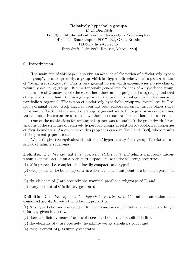
Relatively hyperbolic groups.

B. H. BowditchFaculty of Mathematical Studies, University of Southampton,

Highfield, Southampton SO17 1BJ, Great [email protected]

[First draft, July 1997. Revised, March 1999]

0. Introduction.

The main aim of this paper is to give an account of the notion of a “relatively hyper-bolic group”, or more precisely, a group which is “hyperbolic relative to” a preferred classof “peripheral subgroups”. This is very general notion which encompasses a wide class ofnaturally occurring groups. It simultaneously generalises the idea of a hyperbolic group,in the sense of Gromov [Gro] (the case where there are no peripheral subgroups) and thatof a geometrically finite kleinian group (where the peripheral subgroups are the maximalparabolic subgroups). The notion of a relatively hyperbolic group was formulated in Gro-mov’s original paper [Gro], and has been has been elaborated on in various places since,for example [Fa,Sz]. Many results relating to geometrically finite groups in constant andvariable negative curvature seem to have their most natural formulation in these terms.

One of the motivations for writing this paper was to establish the groundwork for ananalysis of the structure of relatively hyperbolic groups in relation to topological propertiesof their boundaries. An overview of this project is given in [Bo8] and [Bo9], where resultsof the present paper are used.

We shall give two equivalent definitions of hyperbolicity for a group, Γ, relative to aset, G, of infinite subgroups.

Definition 1 : We say that Γ is hyperbolic relative to G, if Γ admits a properly discon-tinous isometric action on a path-metric space, X , with the following properties:

(1) X is proper (i.e. complete and locally compact) and hyperbolic,

(2) every point of the boundary of X is either a conical limit point or a bounded parabolicpoint,

(3) the elements of G are precisely the maximal parabolic subgroups of Γ, and

(4) every element of G is finitely generated.

Definition 2 : We say that Γ is hyperbolic relative to G, if Γ admits an action on aconnected graph, K, with the following properties:

(1) K is hyperbolic, and each edge of K is contained in only finitely many circuits of lengthn for any given integer, n,

(2) there are finitely many Γ-orbits of edges, and each edge stabiliser is finite,

(3) the elements of G are precisely the infinite vertex stabilisers of K, and

(4) every element of G is finitely generated.

1

Relatively hyperbolic groups

The equivalence of these definitions will be proven in this paper (see Theorem 7.10).We refer to the elements of G as “peripheral subgroups”. The insistence that they be finitelygenerated is rather artificial, though it seems to be needed for certain results. Apart fromthis clause, Definition 1 is easily seen to be equivalent to that given in [Gro]. Definition2 is also equivalent to that of “relative hyperbolicity with bounded coset penetration”described in [Fa]. We thus derive the equivalence of these notions.

The first definition could be viewed as a dynamical characterisation, except that weneed to assume that we are dealing with the boundary of a proper hyperbolic space, andthat the action arises from an isometric action on that space. We suspect that these latterclauses are unnecessary, and that one should be able to give a pure dynamical definitionin terms of “convergence actions”. In [Bo7], this was shown to be the case where there areno peripheral subgroups.

The second definition (which we shall introduce first in this paper) will be phrased for-mally in terms of group actions on sets, which are “cofinite” (i.e. finitely many orbits). Wekeep much of the discussion fairly general. In principle, one could take a similar approachto studying other “geometric” properties of groups relative to a given set of subgroups.The standard (non-relative) case corresponds to those actions where all point stabilisers arefinite. In this case, the interesting geometric properties seem to be quasiisometry invariant,though, in the more general setting, there are natural geometric properties which are notquasiisometry invariant (see Section 4). This approach is extended to group splittings in[Bo8].

Each of the various formulations of relative hyperbolicity have technical advantages inspecific contexts, and each make apparent certain features not apparent from the others.We aim to explore such matters in this paper.

There is also a weaker notion, which we shall refer to here as “weak relative hyperbol-icity”. This is a weakening of Definition 2 above. Let G be a conjugacy invariant collectionof infinite subgroups of a group Γ.

Definition : We say that Γ is weakly hyperbolic relative to G if it admits an action on aconnected graph, K, with the following properties:

(1) K is hyperbolic,

(2) there are finitely many Γ-orbits of edges, and

(3) each element of G fixes a vertex of K, and each vertex stabiliser of K contains anelement of G as a subgroup of finite index.

This gives rise to many more examples (see [Fa,Ger,MasM] and Section 1). However,there seems to be a greater degree of arbitrariness about this definition. In this paper, weshall focus mostly on the stronger definitions.

We briefly elaborate further these definitions, beginning with the dynamical formula-tion. Suppose that a group, Γ, acts by homeomorphism on a perfect metrisable compactum,M . We say that Γ, is a “convergence group” (in the sense of [GehM]) if the induced ac-tion on the space of distinct triples is properly discontinuous. (For further discussion, see[GehM,T2,Fr1,Bo6].) We say that a convergence group is “(minimal) geometrically finite”if every point of M is either a conical limit point or a bounded parabolic point. (For def-

2


initions, see Section 6.) This is a natural generalisation of the Beardon-Maskit definition[BeM]. It has also been considered in this generality in [T3] and [Fr2]. It generalises theclassical formulation of geometrical finiteness described by Ahlfors and Greenberg [A,Gre],see [Bo2,Bo4]. We discuss this further in Section 1.

In this paper, we shall mostly confine ourselves to the case where M is the bound-ary, ∂X , of a complete, locally compact, Gromov hyperbolic space, X . (As alluded toearlier, this assumption might be conjectured superfluous in the case of geometrically fi-nite groups.) If Γ acts properly discontinuously and isometrically on X , then the inducedaction of ∂X is a convergence action. We can thus define an action on X to be “geomet-rically finite” if the induced action on ∂X is geometrically finite in the dynamical sense.If Π ⊆ ∂X is the set of parabolic points, then one can show that Π/Γ is finite. In fact,one can construct a strictly invariant system of horoballs, (B(p))p∈Π, about Π, such that(X \

⋃p∈Π intB(p))/Γ is compact. In this way, we recover a generalisation of the Marden

definition of geometrical finiteness [Mar].

This gives us the first definition of relative hyperbolicity, namely that a group Γis hyperbolic relative to a set of infinite finitely generated subgroups (the “peripheralsubgroups”) if it admits a geometrically finite action on a proper hyperbolic space, wherethese subgroups are precisely the maximal parabolic subgroups. We note immediately thatthe intersection of any two peripheral subgroups is finite, and that there are finitely manyconjugacy classes of peripheral subgroups. Moreover, each peripheral subgroup is equal toits normaliser.

It is primarily in this context that relatively hyperbolic groups arise in nature, and isessentially the formulation given in [Gro]. However, it leaves unresolved certain obviousquestions. Note that, in the case of a hyperbolic group (where G = ∅) the quasiisometryclass of the space X depends only on the group, Γ. This allows us to define the boundary,∂Γ, of Γ as ∂X . In the general situation, however, this is not the case. Indeed, there seemsto be no particularly natural choice of quasiisometry class of space X (except, maybe,if we were only interested in geometrically finite kleinian groups, where one could takeX to be the convex hull of the limit set). However, as we shall discuss in a moment,we can associate to a relatively hyperbolic group, (Γ,G), a space X(Γ), together with ageometrically finite action of Γ, which is canonical up to Γ-equivariant quasiisometry, eventhough the construction is somewhat artificial. This allows us to give a formal definition ofthe boundary, ∂(Γ,G) as ∂X(Γ). One can go on to show that if X is any complete locallycompact hyperbolic space admitting a geometrically finite action of Γ, then the limit setof ∂X is, in fact, Γ-equivariantly homeomorphic to ∂(Γ,G). We thus see that ∂(Γ,G) is aquite natural object to associate to (Γ,G). We frequently view G as part of the structureof Γ, and abbreviate ∂(Γ,G) to ∂Γ.

The proofs of these last assertions will be obtained using the second formulation ofrelative hyperbolicity. We shall phrase this in terms of group actions on sets. To relatethis to what we have said earlier, we take the set to be the peripheral structure, with thegroup acting by conjugation.

Suppose we fix a group, Γ. A “Γ-set” is a set, V , on which Γ acts. We refer to pointsof V as “vertices”. If x ∈ V , we write Γ(x) for the vertex stabiliser. A “pair stabiliser” is asubgroup of the form Γ(x) ∩ Γ(y) for distinct x, y ∈ V . We shall usually assume that pair

3


stabilisers are finite. A “(Γ, V )-graph”, K, is a connected Γ-invariant graph with vertex setV , and with finitely many Γ-orbits of edges. Clearly any graph-theoretical property whichis independent of the choice of K can be viewed as a property of a Γ-set, V . Since anytwo (Γ, V )-graphs are clearly quasiisometric, any quasiisometry invariant property, suchas hyperbolicity, can be viewed as a property of a Γ-set. In view of this, we may define aΓ-set, V , to be “weakly hyperbolic” if some, and hence any, (Γ, V )-graph is hyperbolic.

This notion of weak hyperbolity is equivalent to the formulation of relative hyperbol-icity formulated in [Fa] (without the assumption of finite pair stabilisers) and used, forexample, in [MasM] and [Ger]. However, it is weaker than that in which we are primarilyinterested here. For this we shall need an additional combinatorial hypothesis, which weshall call “fineness”. This is not a quasiisometry invariant. However, it turns out to beindependent of the choice of (Γ, V )-graph.

In the same way that hyperbolicity can be viewed as a geometric weakening of certainproperties of a simplicial tree (such as 0-thin triangles), the notion of fineness can be viewedas weakening of combinatorial properties. Thus, for example, a simplicial tree might bedefined as a connected graph which contains no circuits. We say that a graph is “fine”if there are only finitely many circuits of a given length containing any given edge. Thisseems to be a fairly robust notion, and has several equivalent formulations, as we shall seein Section 2. We can thus define a Γ-set, V , to be “fine” if some (hence any) (Γ, V )-graphis fine.

We shall say that a Γ set, V , is “hyperbolic” if it has finite pair stabilisers, finitelygenerated point stabilisers, and is fine and weakly hyperbolic. This reduces to essentiallytwo cases. If every vertex of V has finite stabiliser, then this is equivalent to saying thatΓ is word hyperbolic in the sense of Gromov. On the other hand, if there exist verticesof infinite degree, then we can assume that every vertex has infinite degree. In the lattercase, we get an equivalent definition of relatively hyperbolic group — if G is a peripheralstructure on Γ, then we can view G as a Γ-set, where the action is by conjugation, andwe can define (Γ,G) to be hyperbolic if G is hyperbolic as Γ-set. A more transparentreformulation of this definition is given by Proposition 4.9.

To relate this to the previous formulation of relative hyperbolicity, we use the complexgiven by Proposition 4.9. This is a Γ-invariant 2-dimensional simplicial complex, K, with0-skeleton V , which has finite quotient under Γ, is locally finite away from V , and is“simplicially hyperbolic”. The last statement means that any cycle of a length n in the1-skeleton bounds a simplicial disc in K with the number of 2-simplices bounded above bya linear function of n. We may “realise” K \ V as a complete locally compact path-metricspace, X(K), by giving each 2-simplex the structure of an ideal hyperbolic triangle, insuch a way that the union of two adjacent triangles is isometric to an ideal hyperbolicsquare. It turns out that X(K) is Gromov hyperbolic, and that the action of Γ on X(K)is geometrically finite. This gives us our space, X(Γ), referred to earlier.

Conversely, suppose we have a geometrically finite action of a group Γ on a completelocally compact hyperbolic space X . Let G be the peripheral structure. We can reconstructa fine hyperbolic graph, K, with vertex set G, as a kind of “nerve” to an invariant set ofhoroballs. More precisely, we take any invariant set of horoballs for Γ, and we connecttwo peripheral subgroups by an edge if the distance between the corresponding horoballs

4


is less than some sufficiently large constant. (Alternatively, if we choose the horoballs tooverlap sufficiently, we can take it to be a nerve in the usual sense.) One verifies that Kis indeed fine and hyperbolic, and that ∂X(K) is Γ-equivariantly homeomorphic to ∂X .

There is a slight complicating factor, which we have not explicitly mentioned. Thisconcerns whether we should assume that the peripheral subgroups are all finitely gen-erated. This is not needed in the discussion of geometrically finite groups in Section 6,but seems to be required, or at least desirable, for the constructions of Sections 3 and4. We shall therefore take it as part of the hypotheses of a relatively hyperbolic group,but not of a geometrically finite group. This necessitates an extra clause in the statementof certain results (for example Proposition 7.9) which has no real mathematical content.(We never need to assume that subgroups of peripheral subgroups are finitely generated.)The assumption of finite generation probably places no significant constraint on the likelyapplications. In certain contexts, one might want to place additional restrictions on theclasses of groups that can arise as peripheral subgroups, for example ruling out any infinitetorsion subgroups. However, we shall have no need to do this here. In the classical contextof geometrically finite groups acting on pinched negatively curved manifolds, all peripheralsubgroups are finitely generated virtually nilpotent.

The outline of this paper is roughly as follows. In Section 1, we shall give examples ofrelatively hyperbolic groups, and relate them to accounts given elsewhere. In Section 2, weconsider a few combinatorial properties of infinite graphs, in particular, introducing thenotion of a “fine” graph. In Section 3, we construct a proper hyperbolic space starting witha fine hyperbolic graph, thereby giving us a notion of boundary for such a graph. In Section4, we study actions of a group, Γ, on a set, allowing us to define the notion of a “hyperbolicΓ-set” and hence of a relatively hyperbolic group. In Section 5, we briefly review hyperboliclength spaces. In Section 6, we study geometrically finite finite actions on proper hyperbolicspaces, largely from a dynamical point of view. In Section 7, we recover fine hyperbolicgraphs from geometrically finite actions, thereby showing that a geometrically finite groupwith finitely generated peripheral subgroups is relatively hyperbolic by the combinatorialdefinition of Section 4. In Section 8, we shall explore properties of fine hyperbolic graphs.In Section 9, we show that the limit set of a geometrically finite group depends, up toequivariant homeomorphism, only on the group and the collection of peripheral subgroups.In Section 10, we describe some basic facts about splittings of relatively hyperbolic groupsover finite subgroups, and how these are observed in the topoology of the boundary.

I would like to thank Pekka Tukia and David Epstein for their comments on thispaper. I am also indebted to Andrzej Szczepanski for his ideas on relatively hyperbolicgroups.

1. Examples.

Before embarking on the formal development of the notion of relative hyperbolicity,we describe a few examples to illustrate the ideas outlined in the introduction. This willalso serve to link these definitions with accounts of the subject given elsewhere. None ofthe rest of the paper is logically dependent on any of the statements made in this section.

5


In order to keep the discussion informal, we shall be a little loose in our terminology.In particular, we shall often speak of a “relatively hyperbolic group” when we really meana group which is hyperbolic relative to a given class of subgroups. In subsequent sections,we shall be more precise.

Perhaps the simplest example of a relatively hyperbolic group is the fundamentalgroup of a once-punctured torus. To understand this geometrically, we give the torus acomplete hyperbolic structure. The choice of such structure is not important, though fordefiniteness, let’s consider the “square torus” obtained by identifying the opposite sides ofan ideal hyperbolic square (in such a way that the endpoints of the common perpendicularto these sides are identified). The topological end of the torus carries the standard geometryof a hyperbolic cusp bounded by a horocycle.

If we lift this picture to the hyperbolic plane H2, we get a regular tessellation of H2

by ideal squares. The preimage of the cusp consists of a collection of disjoint horodiscscentred at the parabolic points, which form a countable dense subset of the ideal circleS1 ≡ ∂H2. We can view the 1-skeleton of the square tessellation as dual to this collectionof horoballs, and hence as combinatorially defining a kind of “nerve” to this set.

The fundamental group, Γ, of the once-punctured torus is free of rank 2. The subgroupsupported by the cusp is infinite cyclic, generated (up to conjugacy) by the commutatorof the free generators. Let G be the set of conjugates of this subgroup. We shall see thatΓ is “hyperbolic relative to G”. In other words, Γ, or more precisely (Γ,G), is a relativelyhyperbolic group. We refer to the elements of G as “peripheral subgroups”.

A more combinatorial picture may be obtained as follows. Start with a euclideansquare torus, puncture it a point, and take the universal cover. Now take the metriccompletion of the resulting locally euclidean space with the induced path-metric. Thisspace may alternatively be constructed as a square complex, by glueing together euclideansquares in the same combinatorial pattern as that of the hyperbolic tessellation just de-scribed. Of course, this complex is not locally finite — the link of each vertex is the realline. From the treelike nature in which the squares are glued together, it is easily verified(via the “thin triangle” property) that the space is hyperbolic in the sense of Gromov.Since it not locally compact, we cannot expect its boundary to be compact. In fact, theboundary is homeomorphic to the set of irrational points of the circle in the subspacetopology.

We remark that this square complex is, in fact, quasiisometric to a (simplicial) tree.However, such a quasiisometry cannot be made Γ-equivariant (as can be seen from Bass-Serre theory), and so cannot be constructed in a particularly natural manner.

In any case, the geometry of the square complex is quite different from that of thehyperbolic plane. Up to quasiisometry, the former can be given a number of different de-scriptions. For example, it can be obtained by taking the hyperbolic picture and collapsingeach horodisc to a point — effectively dragging each parabolic point into the interior andthereby removing them from the boundary. (It is the whole circle S1 which we shall wantto define to be the boundary of the relatively hyperbolic group, (Γ,G).) It is also, of course,quasiisometric to its 1-skeleton, which we have already interpreted as a kind of nerve to thecollection of horodiscs. It is also worth remarking that if we equivariantly add a diagonalto each square, we obtain the graph commonly known as the Farey graph. We shall return

6


to this point later.

Yet another way of viewing this construction, up to quasiisometry, is via the Cayleygraph (or any connected graph on which Γ acts with finite stabilisers and finite quotient).Let K be such a graph. Choose any peripheral group, G ≤ Γ, and let KG be any G-orbitin K. Extend this construction Γ-equivariantly, so that KgGg−1 = gKG for g ∈ Γ. We canarrange that the sets KG are disjoint and collapse each KG to a point. Alternatively, wecan “cone off” each set KG by introducing a cone vertex, vG, and connecting each point ofKG to vG by an edge of unit length. These spaces are again quasiisometric to the squarecomplex. This process is described in [Fa].

The once-punctured torus group is an example of a geometrically finite kleinian group.This notion has its origins in the work of Ahlfors and Greenberg [A,Gre]. Since then, severaldifferent formulations have been given, in particular, by Marden, Beardon and Maskit, andThurston. For some discussion of this, see, for example, [Bo2]. One definition demandsthat the convex core (the quotient of the convex hull of the limit set, or to be more precise,some ε-neighbourhood thereof) has finite volume. (To make this work, we need to placea bound on the order of the torsion elements, see [Ha].) Another way of viewing this isto note that the convex core consists of a compact set together with a finite number ofexponentially tapering cusps. In terms of the convex hull of the limit set, these cuspsarise as quotients of horoballs. We are thus in a similar situation to that described for thepunctured torus. Once again, the group is hyperbolic relative to the maximal parabolicsubgroups, which in this situation are always finitely generated virtually abelian. Theboundary of the group may be naturally identified with the limit set.

The above discussion generalises essentially unchanged to pinched hadamard manifolds[Bo4]. (We need to be careful to take the closed convex hull in this case.) The peripheralsubgroups are now all finitely generated virtually nilpotent [Bo3].

In [Gro], Gromov suggested generalising this to proper (complete, locally compact)hyperbolic path-metric spaces. The hyperbolic space, X , plays the role of the closed convexhull of the limit set in previous examples. The peripheral subgroups are again the maximalparabolic subgroups. The quotient space is quasiisometric to a finite wedge of infinite rays— one ray for each conjugacy class of peripheral subgroup — which correspond to the cuspsin the earlier picture. It is this general picture which will serve as (an equivalent to) thedefinition of relative hyperbolicity in this paper. It will be discussed in detail in Section 7.The only general constraint the definition as stated places on peripheral subgroups is thatthey be countable. However we shall add a clause insisting that they be finitely generated.We can identify the boundary of the group with the ideal boundary of X .

Examples of this more general situation may be obtained as follows. Take n copiesof the ideal hyperbolic triangle, and glue them all together via the identity along theirboundaries. If n = 2, we get the thrice punctured sphere. In general we get a locallyCAT(−1) space (see, for example [GhH]), so its universal cover is globally CAT(−1) andhence hyperbolic. The fundamental group is free of rank 2n − 2. There are 3 conjugacyclasses of peripheral subgroups, each free of rank n− 1. More interesting examples of thistype are explored in [GaP].

Starting with Gromov’s formulation of relatively hyperbolic group, we can constructthe “nerve” to the set of horoballs as an abstract graph, whose vertex set is the set of

7


horoballs and with two horoballs connected by an edge if they are at most a (sufficientlylarge) bounded distance apart. As before, this graph is quasiisometric to the coned-offCayley graph. One can show that such a graph is hyperbolic. This weaker condition servesas a definition of relative hyperbolicity in [Fa]. We shall term it “weakly hyperbolic” inthis paper. To recover Gromov’s definition, one needs to observe that the nerve has anadditional combinatorial property which we shall term “fineness”. For hyperbolic graphs,this is equivalent to what Farb calls “bounded coset penetration”. (This is not hard tosee, though we shall not give a proof here.) As we shall see in Section 3, this is sufficientto reconstruct a proper hyperbolic space, and so gives rise to an equivalent formulationof relative hyperbolicity. In other terminology, we deduce that “relatively hyperbolic”in our sense (i.e. that of Gromov) is equivalent to “relatively hyperbolic with boundedcoset penetration” in the sense of Farb. (We shall insist that peripheral subgroups arefinitely generated — things get a bit complicated without this.) We remark that Farb [Fa]shows that such groups are biautomatic provided that all the peripheral subgroups arethemselves biautomatic, thereby generalising the result of Epstein for geometrically finitekleinian groups.

It is natural to ask what happens if one drops the assumption of local compactness ofthe space, X , in Gromov’s formulation. Again, the nerve of the horoball collection will behyperbolic, but not necessarily fine. It remains the case that each element of G is equal toits normaliser, and any two elements of G intersect in a finite group. It is also natural toinsist that G is a union of finitely many conjugacy classes of subgroups.

An example of such a space can be obtained by gluing together ideal triangles asbefore, except that this time, we take n to be the countably infinite cardinal. In this case,the peripheral subgroups are all infinitely generated free groups. By embedding them infinitely generated groups, one can also construct examples where the peripheral subgroupsare all finitely generated.

We can get a still more general notion, called “weakly hyperbolic” here, by simplydemanding that the coned-off Cayley graph of the group Γ be hyperbolic. This is the maindefinition in [Fa]. (One doesn’t really need that Γ be finitely generated for this. A moreprecise definition is given in Section 3.) In this case, G, need not be a peripheral structurein the strict sense — the intersection of peripheral subgroups might be very large. Thisgives rise to many more examples.

For example, Z2 is weakly hyperbolic relative to any infinite subgroup. More generally,if Γ is any group, and G is any normal subgroup, then Γ is weakly hyperbolic relative toG if and only if Γ/G is hyperbolic.

Another class of examples is described in [Ger]. Suppose that Γ is a hyperbolic group,and that G is a collection of quasiconvex subgroups which is a finite union of conjugacyclasses. Then, Γ is weakly hyperbolic relative to G. Moreover, if it happens that eachelement of G is equal to its normaliser, and the pairwise intersecion of elements of G arefinite, then it follows that Γ is hyperbolic relative to G. This will be proven is Section 7(Proposition 7.11). A proof of the “weakly hyperbolic” statement was presented in [Ger]using other methods, though the argument described there contains a gap (which does notaffect the remainder of that paper).

Other examples are described in the paper of Masur and Minsky [MasM]. These are

8


based on the curve complexes of Harvey (or variations thereof). Let S be an orientablehyperbolic surface of finite type. Choose any natural number, m ∈ N, and let K be thegraph whose vertex set is the set of non-trivial homotopy classes of non-peripheral simpleclosed curves on S, and with two such curves joined by an edge in K if their geometricintersection number is at most m. Up to quasiisometry, this construction is independent ofm — unless S is a once-punctured torus and m = 0. (Note that for a once-punctured torus,and m = 1, we get the Farey graph again.) In [MasM], it is shown that K is hyperbolic.From this, one may conclude that a mapping class group is weakly hyperbolic relative toa class of (direct products of) simpler mapping class groups.

Despite the existence of such examples, we shall not pursue the notion of weak hy-perbolicity in detail in this paper. However many of the arguments and results will beapplicable to that case.

2. Graph theory.

The main aim of this section will to be to introduce the notion “fineness” of a graph.We develop some basic properties of fine graphs, and describe some simple graph theoreticaloperations that preserve fineness. Additional properties of fine hyperbolic graphs will beexplored in Section 8. We begin by recalling some facts from elementary graph theory.

Let K be a graph with vertex set V (K) and edge set E(K). We can think of K asa 1-dimensional simplicial complex. (We are not allowing loops or multiple edges.) Wewrite V0(K) and V∞(K) respectively for the sets of vertices of finite and infinite degree.A path of length n connecting x, y ∈ V is a sequence, x0x1 . . . xn of vertices, with x0 = xand xn = y, and with each xi equal to or adjacent to xi+1. It is an arc if the xi areall distinct. A cycle is a closed path (x0 = xn), and a circuit is a cycle with all verticesdistinct. We regard two cycles as the same if their vertices are cyclically permuted (i.e.x0x1 . . . xn−1x0 = xkxk+1 . . . xk for all k). We frequently regard arcs and circuits assubgraphs of K. Two arcs are independent if they meet only in their endpoints. We speakof two paths or subgraphs as distinct simply to mean that they are not identical. Thelength of a subgraph is the cardinality of its edge set.

We put a path metric, dK , on V (K), where dK(x, y) is the length of the shortest pathin K connecting x to y. (We set dK(x, y) = ∞ if there is no such path.) When we speakof a subset of V (K) as being bounded we mean with respect to this metric.

If A ⊆ V (K), we write K \A for the full subgraph of K with vertex set V (K) \A, i.e.the graph obtained by deleting the vertices A together will all incident edges. If x ∈ K,we abbreviate K \x to K \x. We say that K in n-vertex-connected if K \A is connectedfor any subset, A, of V (K), of cardinality strictly less than n. (We are breaking withtradition slightly in that we are deeming the complete graph on n vertices to be n-vertexconnected.)

Let K be a connected graph. A block of K is a maximal 2-vertex-connected subgraph.Two blocks meet, if at all, in a single vertex. The block tree of K is the bipartite graphwhose vertex set is defined as the abstract union of the set, V , of vertices of K and the set,B, of blocks of K, where a vertex, x, is adjacent to a block, B, in the block tree if x ∈ B

9


in K. It’s not hard to see that the block tree is indeed a simplicial tree (i.e. a connectedgraph with no circuits).

So far, everything we have said is standard elementary graph theory. We now moveon to some less standard definitions.

Definition : A collection, L, of subgraphs of K is edge-finite if L ∈ L | e ∈ E(L) isfinite for each edge e ∈ E(K).

Definition : A subset A ⊆ V (K) is locally finite in K if every bounded subset of A isfinite.

If x ∈ V (K), we write VK(x) ⊆ V (K) for the set of vertices adjacent to x.We are now ready for the main result of this section:

Proposition 2.1 : Let K be a graph. The following are equivalent:

(F1): For each n ∈ N, the set of circuits in K of length n is edge-finite.

(F2): For all x, y ∈ V (K) and n ∈ N, the set of arcs of length n connecting x to y is finite.

(F3): For any x, y ∈ V (K) and n ∈ N, there does not exist an infinite collection of pairwiseindependent arcs of length n connecting x to y.

(F4): Suppose x, y ∈ V (K) are any pair of distinct vertices, and n ∈ N. If L is anyedge-finite collection of connected subgraphs of K of length n, each containing both x andy, then L is finite.

(F5): For each vertex x ∈ K, the set VK(x) is locally finite in K \ x.

Proof : We prove (F2) ⇒ (F1) ⇒ (F3) ⇒ (F2), (F2) ⇒ (F4) ⇒ (F3) and (F2) ⇒ (F5)⇒ (F3).

(F2) ⇒ (F1): Suppose e ∈ E(K) has endpoints x, y ∈ V (K). Each circuit, γ, of length ncontaining e gives us an arc, γ \ e, of length n − 1 connecting x and y. There can only befinitely many such arcs, and hence only finitely many such circuits.

(F1) ⇒ (F3): Suppose, for contradiction, that there is an infinite collection, (βi)i∈N, ofpairwise independent arcs of length n connecting the same pair of distinct points. Let e beany edge of β0. Now, for each i, β0 ∪βi is a circuit of length 2n containing e, contradicting(F1).

(F3) ⇒ (F2): Suppose, for contradiction, that (F2) fails. Let n ∈ N be minimal such thatthere exist distinct points, x, y ∈ V (K) and an infinite collection, (βi)i∈N, of distinct arcsof length at most n connecting x to y.

We claim that only finitely many of the βi contain any given point, z ∈ V (K)\x, y.To see this, note that z divides any such arc, βi, into two subarcs, β−

i and β+i , each of

length at most n − 1, and connecting x to z and z to y respectively. From the minimalityof n, we see that there are only finitely many possibilities for β−

i and β+i , and hence for

βi, as claimed. It follows, more generally, that if A ⊆ V (K) \ x, y is any finite set, theni ∈ N | βi ∩ A 6= ∅ is finite.

10


We can thus, inductively, pass to a subsequence, (βij)j , such that βij

meets no point of⋃k<j V (βik

)\x, y. In other words, (βij)j is an infinite collection of pairwise independent

arcs of length at most n, connecting x to y. This contradicts (F3).

(F2) ⇒ (F4): Suppose, for contradiction, that (Li)i∈N is an edge-finite collection of con-nected subgraphs of k, each of length n, and each containing a pair of distinct points,x, y ∈ V (K). Now, we can inductively pass to a subsequence, (Lij

)j of subgraphs whichare pairwise edge-disjoint (since only only finitely many graphs, Li, contain any of thefinite set,

⋃k<j E(Lik

), of edges of K). Now, let βj be any arc in Lijconnecting x to y.

These arcs are all edge-disjoint, and so, in particular, are distinct. Moreover, they all havelength at most n, contradicting (F2).

(F4) ⇒ (F3): Clearly, any collection of independent arcs connecting a pair of points willbe edge-disjoint, and hence finite by (F4).

(F2) ⇒ (F5): Suppose, for contradiction, that x ∈ V , and that VK(x) is not locally finitein K \ x. In other words, we can find some y ∈ VK(x), and some n ∈ N, such that there isan infinite sequence, (zi)i∈N, of distinct points in VK(x), each a distance at most n fromy. Let αi be a shortest path in K \ x from y to zi, and let βi be α concatenated with theedge zix. We see easily that βi is an arc of length at most n + 1 connecting y to x. Sincezi ∈ V (βi), these arcs are all distinct, contradicting (F2).

(F5) ⇒ (F3): Suppose, for contradiction, that there exist points x, y ∈ V , and an infinitesequence, (βi)i∈N of pairwise independent arcs of length n connecting x to y. Let zi be thefirst vertex of the arc βi after x, and let αi be the subarc of βi connecting zi to y. Thus,zi ∈ VK(x), and αi has length n − 1 and lies in K \ x. We see that any pair of points,zi and zj are connected by a path of length 2(n − 1) in K \ x. Thus, zi | i ∈ N is aninfinite subset of VK(x), which is bounded in K \ x, contradicting (F5). ♦

Definition : We say that a graph is fine if it satisfies one, hence all, of the properties(F1)–(F5) featuring in Proposition 2.1.

We first make some trivial observations about fineness. The proofs are easy.

Lemma 2.2 : Any subgraph of a fine graph is fine. Any locally finite graph is fine. Agraph is fine if and only of each of its components is fine. A connected graph is fine if andonly if each of its blocks is fine. ♦

Another point to note is that a 2-vertex-connected fine graph is countable. Thisfollows, since in this case, every vertex has countable degree by property (F5).

We want to describe some slightly less trivial operations on graphs which preservefineness. To this end, the following lemma will be useful.

Let K be a graph. Given an arc, α, in K, we write e(α) for the unordered pairof endpoints of α. If A is a set of arcs, we write K[A] for the graph with vertex setV (K[A]) = V (K), and edge set, E(K[A]) = E(K) ∪ e(A) | α ∈ A. (This union neednot be disjoint — if α has length 1, then e(α) is already in E(K).)

11


Lemma 2.3 : Suppose that K is a fine graph, and A an edge-finite collection of arcs ofbounded length in K. Then, K[A] is fine.

Proof : Let k be the maximal length of any arc in A. Suppose that L is a connectedsubgraph of K[A] of length n. We may associate to L, a connected subgraph, L′, of K,with V (L) ⊆ V (L′), and of length at most kn, as follows. For each edge, e ∈ E(L), wechoose some α ∈ A with e = e(α), and let L′ be the union of all such arcs. (That is thesubgraph consisting of all vertices and all edges of such arcs. If E(L) happens to be empty,then we set L′ = L.)

We claim that if L is an edge-finite collection of connected subgraphs of K[A], thenL′ = L′ | L ∈ L is edge-finite in K. To see this, fix some edge e ∈ K. Now, A(e) =α ∈ A | e ∈ E(α) is finite, and so E(e) = e(α) ∈ E(K[A]) | α ∈ A(e) is finite. Now,if e ∈ E(L′) for some L ∈ L, we see that E(e) ∩ E(L) 6= ∅. Since E(e) is finite, and L isedge-finite, we see that the set of such L ∈ L is finite. This shows that L′ is edge-finite asclaimed.

Now, suppose that x, y ∈ V (K[A]) = V (K) are distinct, and that L is an edge-finitecollection of connected subgraphs of K[A] of bounded length containing x and y. We seethat L′ is an edge-finite collection of subgraphs of K of bounded length containing x andy. By (F5), it follows that L′ is finite. But only finitely many graphs in L can give rise toa given graph is L′, so it follows that L is finite. This verifies property (F5) for K[A]. ♦

More generally, suppose that L is any edge finite collection of subgraphs of boundedlength. Let A be the set of arcs which lie inside some graph in L. Clearly this collectionis also edge-finite. Let K[L] = K[A]. In other words, for every L ∈ L, we span V (L) by acomplete graph. By Lemma 2.3, we get:

Lemma 2.4 : Suppose that K is fine, and that L is an edge-finite collection of connectedsubgraphs of bounded length. Then, K[L] is fine. ♦

If L ∈ L, we write F (L) for the full subgraph of K[L] with vertex set V (L). Thus,F (L) is complete. We also see easily that the collection, F (L) | L ∈ L is edge finite (usingproperty (F4)). Thus, for many purposes, we take an edge-finite collection of subgraphsof bounded length to consist entirely of complete subgraphs.

We shall use Lemma 2.4 in a number of constructions, three of which we describebelow.

Let K be any graph, and n ∈ N. We construct a graph Kn, with vertex set, V (Kn) =V (K), by connecting distinct x, y ∈ V (Kn) by an edge in Kn if and only if either xy ∈E(K) or x and y lie in some circuit in K of length at most n. Clearly, K ⊆ Kn.

If we write L for the set of circuits of length at most n in K, we get that Kn = K[L].It thus follows from Lemma 2.4 that:

Lemma 2.5 : If K is fine, then Kn is fine for all n ∈ N. ♦

The next operation we consider is that of “binary subdivision”. Suppose that K isa graph. If e ∈ E(K), we can subdivide e into two edges by inserting an extra vertexat the “midpoint”, m(e), of e. If we do this for each edge of K, we obtain a graph, L,

12


whose realisation is identical to that of K. We now form a graph, K ′, containing L, withvertex set V (K ′) = V (L), by connecting two midpoints, m(e1) and m(e2) by a new edgewhenever there exists a third edge e3 ∈ E(K) such that e1, e2, e3 forms a 3-circuit in K.We refer to K ′ as the binary subdivision of K.

Another way to express this construction is to define the “flag 2-complex”, Σ(K),associated to a graph K. This is the 2-dimensional simplicial complex with 1-skeleton K,and with a set of three vertices of K spanning a simplex in Σ(K) if and only if they forma 3-circuit in K. (Note that, if K is fine, then Σ(K) is locally finite on the complement ofthe set of vertices.) Now, Σ(K ′) is obtained from Σ(K) by dividing each edge in two, anddividing each 2-simplex into four smaller simplices. (Figure 1.) Note that the realisationof the flag 2-complex remains unchanged.

Lemma 2.6 : If K is fine, then so is the binary subdivision, K ′.

Proof : Let L be the graph obtained by dividing each edge of K in two. The circuits of Lare of even length and correspond precisely to circuits of half their length in K. It followsthat L is fine. Now, K ′ ⊆ L6, and so, by Lemma 2.5, we see that K ′ is fine. ♦

Suppose that A ⊆ V (K) and n ∈ N. We define a graph K(A, n), with vertex setV (K(A, n)) = A, and with x, y ∈ A joined by an edge in K(A, n) if and only if there existsan arc, α, of length at most n in K, with α ∩ A = x, y. Recall that V∞(K) ⊆ V (K) isthe set of vertices of infinite degree in K.

Lemma 2.7 : Suppose that K is fine, V∞(K) ⊆ A ⊆ V (K), and n ∈ N. Then, K(A, n)is fine.

Proof : Let A be the set of arcs of length at most n in K meeting A precisely in theirendpoints. Since each vertex of V (K)\A has finite degree, we see easily that there are onlyfinitely many possibilities for such arcs passing through any given edge. In other words, Ais edge-finite. Thus, by Lemma 2.4, K([A]) is fine. Now, K(A, n) is obtained from K[A]by deleting the isolated vertices V (K) \ A. It follows that K(A, n) is fine. ♦

In relation to the last construction, we should make a simple observation for futurereference.

Definition : A subset, A ⊆ V (K) is r-dense if every vertex of K is a distance at most rfrom some point of A.

The following is easily verified:

Lemma 2.8 : If K a connected graph, and A ⊆ V (K) is r-dense, then K(A, 2r + 1) isconnected. ♦

We finish this section with another construction which preserves fineness. We firstmake a trivial observation:

13


Lemma 2.9 : Suppose that K is a graph and A ⊆ V (K). Suppose that every point ofA has degree 0 or 1 in K. If K \ A is fine, then so is K.

Proof : By property (F1), since every circuit of K lies in K \ A. ♦

Suppose that (Li)i∈I is a collection of subgraphs of a graph K, indexed by a set I.We say that (Li)i∈I is “edge-finite” if the set Li | i ∈ I is edge-finite, and only finitelymany Li are equal to any given subgraph. In other words, i ∈ I | e ∈ E(Li) is finite forevery edge e ∈ E(K).

Lemma 2.10 : Suppose that K is a graph, n ∈ N, and A ⊆ V (K). Suppose thatfor each x ∈ A, there is a connected subgraph L(x) ⊆ K \ A, of length at most n, andcontaining every vertex adjacent to a in K. If K \ A is fine, and the collection (L(x))x∈A

is edge-finite, then K is fine.

Proof : We may as well suppose that K is connected. Let M be a subgraph of K withV (M) = V (K), which contains K \A, and such that every element of A has degree 1 in M .Given x ∈ A, let L′(x) be the subgraph of M consisting of L(x) together with the uniqueedge of M incident on x. Thus, L′(x) is connected, and has length at most n + 1, andvertex set V (L(x)) ∪ x. Now, it’s clear that the collection (L′(x))x∈A is an edge-finitecollection of subgraphs of M . Let L = L′(x) | x ∈ A. By Lemma 2.4, M [L] is fine. Butnow, K is naturally embedded as a subgraph M [L], and so K is fine as claimed. ♦

Fine graphs without finite order vertices have the property that geodesic arcs areextendible. More precisely:

Proposition 2.11 : Suppose that K is a fine graph with every vertex of infinite degree.Any finite geodesic arc in K lies inside an biinfinite geodesic arc.

Proof : It’s enough to show that if x, y ∈ V (K), then there is some z ∈ V (K) adjacentto y such that dK(x, z) = dK(x, y) + 1. To see this, note that if z is adjacent to y, anddK(x, z) ≤ dK(x, y), then the edge xz together with any geodesic from x to z is an arc oflength at most dK(x, y)+1 connecting x to y. There are only finitely many such arcs, andhence only finitely many such z. ♦

We remark that, throughout this section, we could equally well have worked insteadwith a notion of “uniform” fineness, where we bound the number of circuits of a givenlength through any given edge etc. In the group theoretical applications, all the finegraphs we work with will be uniformly fine in this sense.

3. Hyperbolic graphs and complexes.

In this section, we explore the notion of hyperbolicity of graphs and related spaces.One of the main objectives will be to associate a space, X(K), to a graph, K, which willbe hyperbolic under suitable hypotheses on K (see Theorem 3.8).

14


For the present purposes, we shall define hyperbolicity in terms of the linear isoperi-metric inequality. Our discussion here is essentially combinatorial, though it will be conve-nient to phrase certain ideas in terms of CW-complexes. We shall look at other aspects ofhyperbolicity in Section 5. Specific properties of fine hyperbolic graphs will be consideredfurther in Section 8.

Suppose that K is a connected graph, and that n ∈ N. We write Ωn(K) for theCW-complex obtained by gluing a 2-cell to every circuit of length at most n in K. (ThusK is fine if and only if, for all n ∈ N, Ωn(K) is locally finite away from V (K).)

Definition : We say that K is n-simply connected if Ωn(K) is simply connected. We saythat K is coarsely simply connected if it is n-simply connected for some n.

Clearly a graph is n-simply connected if and only if each of its blocks is.

We can define the notion of hyperbolicity in similar terms using “cellular discs”. By acellulation of a space, we mean a representation of the space as a CW-complex. A cellularmap between CW-complexes is one which sends cells into (possibly lower dimensional)cells. (This is more restrictive than the definition of “cellular map” commonly given inthis context.) We can think of a cycle in K as consisting of a cellulation of the circle, S1,together with a cellular map of S1 into K which sends each 1-cell homeomorphically ontoan edge of K. We can define a cellular disc, (D, f), (of coarseness n) as consisting of acellulation of the disc, D, together with a map, f , of the 1-skeleton of D into K such thatthe boundary of each 2-cell in D has at most n 1-cells and gets mapped to a cycle (of lengthat most n) in K. We measure the area of D (or of (D, f)) as the number of 2-cells in D.We speak of (D, f) as a (cellular) spanning disc for the cycle f |∂D, and of the cycle f |∂Das bounding (D, f). Note that we can extend f to a cellular map f : D −→ Ωn(K), whichgives us a more intuitive way of thinking about such an object. (There are a multitude ofother ways of formulating the notion of “spanning disc” and “area”, and we shall see slightvariations on these later. All we really require of such a notion is that it should satisfy a“rectangle inequality” — see, for example, [Bo1] for some discussion.)

There is another technical point we should make, namely that one can reformulateeverything we say using circuits in place of cycles. This is based on the following simpleobservation. Suppose β is a cycle in K. Then, we can find a cellulation of the disc, D, withthe number of 2-cells bounded by fixed linear function of length(β), and an extension ofβ to the 1-skeleton of D, such that the boundary of each 2-cell in D is either collapsed toan edge or point of K, or mapped onto a circuit. This can be achieved inductively. If twovertices of β get mapped to the same vertex of K, then we split β into two subcycles byconnecting these two vertices by an edge which gets collapsed to a point in K. (Note thatthis process need not give us a spanning disc, since we have no control over the lengths ofthese circuits.)

We now equip our graph K with its path metric, dK , obtained by assigning each edgea length 1. The following is one expression of the linear isoperimetric inequality:

Proposition 3.1 : A connected graph K is hyperbolic if and only if there is somen ∈ N, and a fixed linear function, such that every cycle in K has a cellular spanning disc

15


of coarseness n, whose area is bounded by the given linear function of the length of thecycle. ♦

The number n together with the linear function will be referred to as “hyperbolicityparameters”.

From the earlier observation, we see that we could replace the word “cycle” by “circuit”in the this proposition. An immediate consequence of this is that a connected graph ishyperbolic if and only its blocks are uniformly hyperbolic (i.e. with fixed hyperbolicityparameters). We also note that hyperbolic graph is coarsely simply connected.

For some purposes, it is better to define hyperbolicity in terms of simplicial complexes,rather than cell complexes.

By a flag 2-complex , we shall mean a 2-dimensional simplicial complex with the prop-erty that every 3-circuit in the 1-skeleton bounds a 2-simplex. Prior to the statementof Lemma 2.6, we defined the flag complex, Σ(K), associated to a graph, K, which wemay identify with Ω3(K). Thus, Σ(K) is simply connected if and only if K is 3-simplyconnected. We note:

Lemma 3.2 : If K is n-simply connected, then Kn is 3-simply connected. ♦

(Here Kn is the graph defined in Section 2.)We also get a combinatorial notion of hyperbolicity.

Definition : A simplicial disc, (D, f), in K, consists of a triangulation of the disc D,together with a simplicial map, f , of D into Σ(K). We speak of (D, f) as a (simplicial)spanning disc bounding the cycle f |∂D in K. We measure the area of (D, f) as the numberof 2-simplices in the triangulation of D.

Definition : We say that a connected graph, K, is simplicially hyperbolic if there is afixed linear function such that every cycle in K bounds a simplicial disc, whose area isbounded by this linear function of the length of the cycle.

As before, we can replace the word “cycle” by “circuit”, without changing the defini-tion. A graph is simplicially hyperbolic if and only if its blocks are uniformly simpliciallyhyperbolic. A simplicially hyperbolic graph is obviously 3-simply connected.

Note that if β is a circuit, then we can assume that a simplicial spanning disc, (D, f),,maps ∂D homeomorphically to β.

Clearly this notion has combinatorial as well as geometric content — it is certainlynot a quasiisometry invariant. However, we note:

Lemma 3.3 : If K is hyperbolic, then Kn is simplicially hyperbolic for some n. ♦

The following discussion of links in K is only indirectly relevant to the main objectiveof this section (the construction of the space X(K)). However it will help to clarify certainpoints arising.

Let K be any graph, and x ∈ V (K). Recall that VK(x) ⊆ V (K) is the set of verticesadjacent to x. Let LK(x) be the full subgraph of K with vertex set VK(x). Thus LK(x)

16


is precisely the link of x in Σ(K). The following is a simple exercise:

Lemma 3.4 : If K is 2-vertex-connected and 3-simply connected, then LK(x) is con-nected for each x ∈ LK(x). ♦

(It follows that the space Σ(K) \ V (K) is connected.) The proof of Lemma 3.4 isessentially the same as that of the following result.

If L is a connected subgraph of K, we say that L is linearly distorted if given anyx, y ∈ V (L), dL(x, y) is bounded above by some fixed linear function (the distortion bound)of dK(x, y).

Lemma 3.5 : If K is 2-vertex-connected and simplicially hyperbolic, then LK(x) islinearly distorted in K \x for all x ∈ V (K). Moreover, the distortion bound is independentof x ∈ V (K).

Proof : Suppose y, z ∈ L = LK(x) are distinct. Let β be an arc of minimal length, say n,connecting y to z. We see that β ∪ yxz is a circuit of length n + 2 in K. It thus bounds asimplicial disc, f : D −→ Σ(K), whose area is linearly bounded in terms of n. We identify∂D with its image in K. Let S be the star of x. Consider the preimage of the componentof f−1S which contains x/ Its boundary lies in f−1L, is connected, and contains y andz. It follows that there is an arc in f−1L connecting y to z. The length of this arc islinearly bounded in terms of n, and its image in K connects x to y in L. This shows thatL is linearly distorted in K (and indeed that L is connected, as claimed by Lemma 3.4).Moreover, the distorsion bound is uniform. ♦

Note that if Σ(K) is locally finite away from V (K), then LK(x) is locally finite for allx ∈ V (K). It is now a simple consequence of Lemma 3.5 that:

Lemma 3.6 : If K is simplicially hyperbolic and Σ(K) is locally finite away from V (K),then K is fine.

Proof : Note that each block of K is satisfies the same hypotheses, and so, using Lemma3.5, satisfies condition (F5) of fineness. By Lemma 2.2, we see that K is fine. ♦

We remark that the proofs of Lemmas 3.5 and 3.6 have not really used the fact thatΣ(K) is a flag 2-complex. Both lemmas hold if we take Σ to be any simplicially hyperbolic2-complex with 1-skeleton K.

(An indirect proof of Lemma 3.6, can also be given from the construction of the space,X(K), together with the results of Section 7.)

We now assume that K is 2-vertex-connected, and set about the construction of thespace X(K). We can view this as a geometric realisation of the space, Σ(K) \ V (K),which, as we have already observed, is connected. To do this, we take, for each 2-simplexin Σ(K), an ideal hyperbolic triangle. We glue these triangles together by isometry alongtheir edges, in the same combinatorial pattern as Σ(K). There is a canonical way ofperforming these identifications, which may be characterised by saying that the union of

17


two adjacent triangles is isometric to an ideal hyperbolic square. The following is a simpleobservation:

Lemma 3.7 : If K is fine, then X(K) is complete and locally compact.

This will turn out to be the only case of interest to us, though we have no need to imposethe assumption of fineness in what follows.

Our main result will be:

Theorem 3.8 : If K is 2-vertex-connected and simplicially hyperbolic, then X(K) ishyperbolic.

Here, of course, we use “hyperbolic” in the sense of Gromov [Gro], which we shall elaborateon shortly. (See also Section 5.)

In fact we will draw further consequences from our construction, notably that thereis a canonical embedding of V (K) in the ideal boundary, ∂X(K), of X(K). Moreover, apoint of V (K) is isolated in ∂X(K) if and only if it has finite degree in K.

Let’s focus for the moment on showing that X(K) is hyperbolic. We shall needanother notion of spanning disc, appropriate to the present context. The idea is to take ariemannian metric on the disc D and a lipschitz map from D into our space X , where ofcourse, we need to bound the lipschitz constant. However, we need to make allowance forthe fact that X is not simply connected. We thus make do with a riemannian metric on aplanar surface H ⊆ D, bounded by ∂D and a finite number of circles S1, . . . , Sk in D. Weinsist that the lengths of each of these circles is bounded above by some fixed constant.We measure the area of D as the riemannian area plus the sum of the lengths of the curvesSi. A “perforated” spanning disc thus consists of a lipschitz map, f , of H into X . Wespeak of (D, f) as “spanning” the loop f |∂D. It is easily checked that this notion satisfiesthe rectangle inequality as described in [Bo1]. It follows that X is hyperbolic if every loop,β, in X bounds a spanning disc whose area is linearly bounded by length(β).

The following construction is a special case of a more general procedure of taking“cusps” over metric spaces, described in [Gro].

By a spike in the hyperbolic plane, H2, we mean a closed region bounded by twoasymptotic geodesic rays and a horocyclic arc of length 1. More precisely, we can define aspike, Y , as the region [0, 1] × [1,∞) in the upper half-space model. We write Yt ⊆ Y forthe region [0, 1] × [et,∞) (so that Y = Y0). Note that Yt is the intersection of Y with ahorodisc of hyperbolic height t above the horocyclic boundary of Y .

Suppose now that L is a connected graph. We construct a space by taking a spike forevery edge of L, and gluing them together, by isometry along the bounding rays, in thepattern prescribed by L. This gives us a hyperbolic 2-complex denoted cusp(L), with acopy of L embedded in the 1-skeleton as the union of all the horocyclic edges. (Here weuse “hyperbolic” in the sense of hyperbolic geometry.) The remainder of the 1-skeletonconsists of a set of geodesic rays, one for each vertex of L. These rays are asymptotic,in the sense that the distance between any two of them is bounded. We can thus embedcusp(L) is a hausdorff topological space, cusp(L) ∪ p, by adjoining an “ideal point”,

18


p, which compactifies each of these rays. A neighbourhood base of p is given as thecomplements of bounded subsets of cusp(L). (In the case of particular interest, where L islocally finite, cusp(L) will be complete and locally compact, and we obtain the one-pointcompactification of cusp(L).)

We observe that cusp(L) is hyperbolic (in the sense of Gromov). This is readily seenby spanning a loop, β, in cusp(L) simply by coning over the ideal point p. The area of thedisc thus obtained is at most length(β). We have the technical detail that our disc is notentirely contained in our space. However we can easily put this right by making a smallhole in the disc at p, and pushing it into cusp(L). Thus gives us a perforated spanningdisc, in the sense described earlier. This shows that cusp(L) is hyperbolic.

It is now a simple matter to show that the ideal boundary of cusp(L) consists of asingle point which we may identify with our point p. Moreover, L is a horocycle about p.It is also worth observing that the closed subset, Bt ⊆ cusp(L) obtained as the union ofthe sets Yt in the construction of cusp(L), is a horoball about p.

Suppose we subdivide an ideal triangle into four pieces using three horocyclic arcswhich touch pairwise at points on the edges of the triangle, as shown in Figure 2. Wehave the happy coincidence that each horocylic arc has length 1, so that each of the threeunbounded pieces is isometric to a spike, as described earlier. (This saves us the botherof rescaling.) Now, subdividing each triangle of X(K) in this way, we obtain a realisationof Σ(K ′) \ V (K) as a complex with 2-cells locally modelled on the hyperbolic plane. HereK ′ is the binary subdivision of K. Now, if x ∈ V (K), we write S(x) for the star of xin Σ(K ′). Thus, L(x) = LK′(x) is the boundary of S(x) in Σ(K ′). Clearly S(x) \ x isisometric to cusp(L(x)). Note that the interiors of these stars are all disjoint.

Given A ⊆ V (K), recall that K ′ \ A is defined as the full subgraph of K with vertexset V (K ′) \ A. We see that Σ(K ′ \ A) = Σ(K ′) \

⋃x∈A intS(x). Let P = Σ(K ′ \ V (K)).

Thus, V (P ) = V (K ′) \ V (K).

Proof of Theorem 3.8 : Let β be a loop (i.e. a closed rectifiable path) in X(K). Wesuppose that β consists of an alternating sequence of paths, α1, γ1, α2, γ2, . . . , αk, γk, whereeach αi consists of a sequence of edges in the 1-skeleton of P , and each γi is a path of lengthat least 2 in lying in S(xi) for some xi ∈ V (K). (More precisely, we can homotop β tosuch a path, only increasing its length by an amount which depends linearly on the originallength, and such that the area of the homotopy is similarly bounded.) Let yi, zi ∈ V (P )be the endpoints of the path γi. Let γ′

i be the path yixizi in K ′. Let β′ be the path inK ′ obtained from β by replacing each path γi by γ′

i. Thus length(β′) ≤ length(β). Now,by hypothesis, K and hence K ′ is simplicially hyperbolic, and hence bounds a simplicialdisc, D0, whose area (as measured by the number of 2-cells) is linearly bounded in terms oflength(β′). Note that the riemannian area of its image in X(K) (punctured at the verticesV (K)) is certainly less than π times this combinatorial area.

Now, consider the closed path γi ∪ γ′i in S(xi) = cusp(L(xi))∪ xi. As in our earlier

discussion, we see that this spans a disc, Di, of area at most length(γi), obtained byconing over the point xi. We perform this construction for each i = 1, . . . , k. In this way,we obtain a spanning disc, D, for β, by joining each Di to D0 along the arc γ′

i. Note that∑k

i=1 area(Di) ≤∑k

i=1 length(γi) ≤ length(β). We conclude that the total hyperbolic area

19


of D is linearly bounded in terms of length(β).As before, we are left with the technical point that our disc may pass (finitely often)

through points of V (K). However, we can simply puncture the disc at these points andpush it slightly into X(K). Since everything is locally just a cone, we can control thelength of the new boundary curves arising. In this way we get a perforated spanning discin X(K), of the type described earlier. It follows that X(K) is hyperbolic as claimed. ♦

In fact, we see that the hyperbolicity parameters of X(K), depend only on those ofK.

Let ∂X(K) be the ideal boundary of X(K). This is a metrisable topological space. Inthe case of real interest to us, where is X(K) is locally compact, ∂X(K) will be compact,though we have no reason to assume this at present.

Suppose x ∈ V (K). Write S′(x) = S(x)\x, so that S′(x) is isometric to cusp(L(x)).Suppose y ∈ VK′(x). The edge yx (minus the point x) is gives us a ray, β, in S′(x) ⊆ X(K).We parameterise β by arc-length such that β(0) = y. From the intrinsic geometry ofS′(x) = cusp(L(x)), we see easily that β is a geodesic in cusp(L(x)), and that the distanceof β(t) from L(x) is equal to t. Now, L(x) is the boundary of S′(x) in X(K), and soit follows easily that β is, in fact, a geodesic ray in X(K). Now, any two such rays inS′(x) are asymptotic and so define an ideal point, p(x) ∈ ∂X(K). Moreover, we see thatS′(x) is a horoball about p(x) in X(K). In particular it follows (see Section 5) that S′(x)is quasiconvex in X(K). Moreover the constant of quasiconvexity is independent of x.(Another proof of this can be given via Lemma 3.5.) Note that if x 6= y, then it’s easilyseen that p(x) 6= p(y), and so p gives us a canonical embedding of V (K) in ∂X(K).

Let B(x, t) ⊆ S(x) be the subset corresponding to Bt in cusp(L(x)). We see thatB(x, t) is also a horoball about x. Moreover, from the quasiconvexity of S(x), it’s not hardto see that B(x, t) is actually convex for all sufficiently large t (independently of x).

For future reference, it’s worth noting that, given the space X(K) and the collection ofhoroballs, B = B(x, t) | x ∈ V (K) for a fixed t, we can recover the graph K geometricallyas a graph with vertex set B, and with two vertices connected by an edge if the distancebetween them in X(K) is at most (or in this case equal to) 2t. This construction makessense for any hyperbolic space with a collection of horoballs — indeed in any metric spacewith a collection of preferred subsets. We shall make use of this construction in Section 7.

We finish this section with another result which may be proven along similar lines toTheorem 3.8:

Lemma 3.9 : Suppose K is simplicially hyperbolic and A ⊆ V (K). Suppose that thelinks LK(x) are uniformly hyperbolic for x ∈ A. Then, K ′ \ A is hyperbolic.

Proof : Suppose β is a cycle in K ′ \A. Now β bounds a simplicial disc, f : D −→ Σ(K)′,whose area is linearly bounded in terms of length(β). Suppose that U is a component off−1(int S(x)) for some x ∈ A. The closure of U in D is a subcomplex which is a planarsurface. The outer boundary of U is a closed curve whose length is at most the area ofU . Now f maps this boundary component to a cycle in L(x). Since L(x) is hyperbolic,this cycle bounds a cellular disc in L(x), whose area is, in turn, linearly bounded by areaof U . Repacing f |U by this cellular disc, and performing this construction for each such

20


U , we get a cellular disc in K ′ \ A spanning β. We have increased the area by an amountlinearly bounded in terms of the area of D. Thus its total area is still linearly bounded interms of length(β). We have thus verified a form of the linear isoperimetric inequality forK ′ \ A. ♦

4. Groups acting on sets.

In this section, we extend the notions of fineness and hyperbolicity to group actionson sets. This will lead to the first definition of relative hyperbolicity, given at the end ofthis section.

As mentioned in the introduction, the approach of this section could be used to studyother “relative” geometric properties of groups. It is based on the construction of graphswhich play the role of Cayley graphs in the non-relative case (where all point stabilisersare finite).

Certain kinds of relative splittings of groups can be phrased naturally in these terms.This gives a convenient formal setting in which te explore splittings of relatively hyperbolicgroups. For some applications of this, see [Bo8].

Suppose Γ is a group. By a Γ-set , we mean a set, V , on which Γ acts. We shall refer tothe points of V as vertices. Thus, if x ∈ V , we refer to the group, Γ(x) = g ∈ Γ | gx = xas a vertex stabiliser . A pair stabiliser is a subgroup of the form Γ(x)∩Γ(y), where x, y ∈ Vare distinct. We write V = V0tV∞, where V0 and V∞ are, respectively, the sets of verticeswith finite and infinite stabilisers. Clearly these are Γ-invariant. We say that V is cofiniteif V/Γ is finite.

Definition : Given a Γ-set, V , a (Γ, V )-graph is a connected Γ-invariant graph with vertexset V and with finite quotient under Γ.

By having “finite quotient” we mean that there are finitely many Γ-orbits of vertices andedges. (We do not take this to imply that there are no edge-inversions — so there mightbe no well-defined quotient graph.)

We shall say that V is connected if it admits a (Γ, V )-graph. Clearly, a connectedΓ-set is cofinite.

(Note that Γ is itself a Γ-set under left multiplication. In this case, a (Γ, Γ)-graphis precisely a Cayley graph. Clearly, Γ is connected as a Γ-set if and only if it is finitelygenerated as a group.)

Lemma 4.1 : Suppose V is a Γ-set and W ⊆ V is Γ-invariant. If V is cofinite, andW is connected and non-empty, then V is connected. Conversely, if V is connected andV∞ ⊆ W , then W is connected.

Proof : For the first statement, let K be a (Γ, W )-graph, and let V ′ ⊆ V \W be a (finite)Γ-orbit transversal of V \ W . For each x ∈ V ′, connect x to any point of W by an edge,

21


e(x). Let L be the graph with vertex set V and edge set E(K)∪⋃

x∈V ′ Γe(x), where Γe(x)is the Γ-orbit of e(x). We see easily that L is a (Γ, V )-graph.

The second statement follows by a similar argument to Proposition 4.10. ♦

Definition : We shall say that a V -set is of finite type if it is connected and has all pairstabilisers finite, and all vertex stabilisers finitely generated.

Although we are ultimately only interested in Γ-sets of finite type, we shall onlyintroduce these hypotheses as we need them.

We continue our study of Γ-sets with a simple observation.

Lemma 4.2 : Suppose V is a connected Γ-set. Any two (Γ, V )-graphs are quasiisometricvia a Γ-equivariant quasiisometry which restricts to the identity on V . ♦

Thus any quasiisometry invariant property of graphs gives rise to a property of con-nected Γ-sets. An obvious example of this is hyperbolicity, and we shall return to thislater. We shall also see that certain combinatorial properties, notably fineness, are alsoindependent of the choice of graph, despite not being quasiisometry invariant. We beginwith some general observations.

Lemma 4.3 : Suppose that V is a connected Γ-set, and K is a fine (Γ, V )-graph. Thenall edge stabilisers of K are finite if and only if all pair stabilisers of V are finite.

Proof : The “only if” bit is trivial. Conversely, suppose that each edge stabiliser of Kis finite. Clearly the stabiliser of any non-trivial arc is finite. Now, suppose x, y ∈ V aredistinct. We connect x and y by an arc, α, in K. By property (F2) of fineness, the set of(Γ(x) ∩ Γ(y))-images of α is finite. It follows that Γ(x) ∩ Γ(y) is finite, as required. ♦

Lemma 4.4 : Suppose that V is a connected Γ-set with finite pair stabilisers, and K isa (Γ, V )-graph. If L is a Γ-invariant collection of finite subgraphs of K with L/Γ finite,then L is edge-finite.

Proof : If L ∈ L and e ∈ E(K), then g ∈ Γ | ge = e is finite. Thus, only finitely manyΓ-images of L contain the edge e. The result follows since L/Γ is finite. ♦

Lemma 4.5 : Suppose that V is a connected Γ-set with finite pair stabilisers, and Kand L are (Γ, V )-graphs. If K is fine, then so is L.

Proof : Suppose e ∈ E(L). Since K is connected, we can find an arc, α, in K whoseendpoints coincide with those of e, i.e. e = e(α) in the notation of Lemma 2.3. We canperform this construction Γ-equivariantly, giving us a Γ-invariant set, A, of arcs in K withL ⊆ K[A]. Since E(L)/Γ is finite, we see that A/Γ is finite, so A is edge-finite by Lemma4.4. By Lemma 2.3, we see that K[A] and hence also L is fine. ♦

22


Definition : We say that a Γ-set is fine if it is connected, has finite pair stabilisers, andif some (and hence every) (Γ, V )-graph is fine.

An alternative way of formulating this is given by the following lemma:

Lemma 4.6 : A connected Γ-set, V is fine if and only if a (Γ, V )-graph has finite edgestabilisers and finitely many Γ-orbits of n-circuits for any n.

(Here, “a” could be interpreted either as “some” or “every”.)

Proof : Let K be a (Γ, V )-graph. The “if” statement follows from Lemmas 4.3 and 4.4.Conversely, suppose K is fine. Let E0 be a finite set of edges containing an edge from eachΓ-orbit. Now, any n-circuit must have some Γ-image meeting E0. By fineness, there areonly finitely many possibilities for such images. ♦

For many purposes it is convenient (if not essential) to restrict to (Γ, V )-graphs whichare 2-vertex-connected. There is more that one way to justify doing this. In general, notethat if K is a (Γ, V )-graph, then Γ acts on the block tree, T , of K. We thus get a splittingof Γ whose vertex groups are either vertex stabilisers of K, or setwise block stabilisers. Wealso note that if B is a block of K, and Γ(B) is the setwise stabiliser of B, then V (B) is aconnected Γ(B)-set, and B is a (Γ(B), V (B))-graph. Thus, for many purposes, we don’tloose much by restricting to a 2-vertex-connected graph.

Another observation which helps to justify this liberty is the following:

Lemma 4.7 : Suppose that V is a Γ-set of finite type. Then V admits a 2-vertex-connected (Γ, V )-graph.

Proof : Let K be any (Γ, V )-graph. Suppose x ∈ V . Recall that VK(x) is the set ofadjacent vertices. Now Γ(x) acts on VK(x) with finite vertex stabilisers and finite quotient.Since Γ(x) is finitely generated, we can find a connected Γ(x)-invariant graph, H(x), withvertex set VK(x), and with E(H(x))/Γ(x) finite. We can perform this construction Γ-equivariantly for each x ∈ V . Let L be the graph with vertex set V , and with edge setE(L) = E(K) ∪

⋃x∈V E(H(x)). Thus, E(L)/Γ is finite. We see that L is a 2-vertex-

connected (Γ, V )-graph as required. ♦

We also have a converse to Lemma 4.7, though it requires additional hypotheses.Note that since coarse simple connectedness is a quasiisometry invariant, we can speak ofa connected Γ-set as being “coarsely simply connected”.

Lemma 4.8 : Suppose a Γ-set, V , is fine and coarsely simply connected. If V admits a2-vertex-connected (Γ, V )-graph, then it is of finite type.

Proof : In other words, we want to show that all vertex stabilisers are finitely generated.Let K be a 2-vertex-connected (Γ, V )-graph. Since K is coarsely simply connected,

there is some n such that Σ(Kn) is simply connected (Lemma 3.2). Suppose x ∈ V . ByLemma 3.4, the link, LKn(x), of x in Σ(Kn) is connected. Since Kn is fine (Lemma 2.5),

23


LKn(x) is locally finite. Now, Γ(x) acts on LKn(x) with finite edge stabilisers and finitequotient. It follows that Γ(x) is finitely generated. ♦

We are now ready for the main definition of this section.

Definition : We say that a connected Γ-set, V , is weakly hyperbolic if some (hence every)(Γ, V )-graph is hyperbolic (in the sense of Gromov, as described in the Section 3).

Definition : A Γ-set is hyperbolic if it has finite type, and is fine and weakly hyperbolic.

In other words, it admits some fine weakly hyperbolic (Γ, V )-graph with all edge stabilisersfinite and all vertex stabilisers finitely generated.

Since this last definition is a bit cryptic, we give a reformulation in the form of thefollowing proposition:

Proposition 4.9 : A Γ-set, V , is hyperbolic if and only if we can represent V as thevertex set, V = V (Σ), of a Γ-invariant simplicial complex, Σ, such that Γ acts on Σ withfinite edge stabilisers and finite quotient, and such that Σ is simplicially hyperbolic andhas no cut vertex.

From the fact that Σ has finite quotient and finite edge stabilisers, we see immediatelythat it is locally finite away from V (Σ). In the definition, we can replace “simpliciallyhyperbolic” by “hyperbolic” (in the usual geometric sense of Gromov), together with theadditional assumption that there are finitely many Γ-orbits of n-circuits in the 1-skeletonof Σ for any n ∈ N. (In fact, for all n sufficiently large in relation to the hyperbolicityparameters will do.) This latter assumption is, in turn, equivalent to saying that, for anyn, we can place some bound on the area of a simplicial disc spanning any circuit (or cycle)of length n in the 1-skeleton of Σ. It turns out that there is no loss in assuming that Σis a flag 2-complex, i.e. every 3-circuit in the 1-skeleton of Σ bounds a 2-simplex. Theassumption that Σ has no cut vertex corresponds to assuming that all vertex stabilisersare finitely generated. It is questionable how natural this assumption is, though withoutit, we would be lead into a number of complications. This point was also discussed in theintroduction.

Proof of Proposition 4.9 : Suppose V is hyperbolic. By Lemma 3.6, V admitsa 2-vertex-connected (Γ, V )-graph, K. Now, K is hyperbolic, so by Lemma 3.3, Kn issimplicially hyperbolic for some n. Let Σ = Σ(Kn). Since Kn is fine and has finitequotient, we see that that Σ has finite quotient. Since, V had finite pair stabilisers, Σ hasfinite edge stabilisers.

Conversely, suppose V is the vertex set of a 2-complex, Σ, with the properties stated.Let K be the 1-skeleton of Σ. We have already observed that Σ is locally finite away fromV . Thus, by Lemma 3.6, and the subsequent remark, we see that K is fine. By Lemma4.6, V has finite pair stabilisers. By Lemma 4.8, V has finitely generated vertex stabilisers.We see that V is of finite type, fine and weakly hyperbolic, as required. ♦

24


We remark that, from the construction, it is easily seen that the complex, K, givenby Propositon 4.9 can be assumed to contain any given Γ-invariant 2-complex with finitequotient.

We refer to a vertex x ∈ V as having “finite” or “infinite degree” according to whetherΓ(x) is finite or infinite. Recall that V0 and V∞ are, respectively, the sets of vertices offinite and infinite degree.

Proposition 4.10 : Suppose that V is a hyperbolic Γ-set, and that W ⊆ V is a Γ-invariant subset with V∞ ⊆ W . Then, W is a hyperbolic Γ-set.

Proof : Let K be a fine hyperbolic (Γ, V )-graph. We can assume that W 6= ∅, so that Wis r-dense in K. Let L = K(W, 2r+1). By Lemma 2.8, L is connected, and by Lemma 2.7,it is fine. Also, from its description as K[A] for an edge-finite arc system, A, (after deletingthe vertices of V \ W ), we see that is has finite quotient. Thus, L is a (Γ, W )-graph. Wesee that W is fine. Since K and L are quasiisometric, we see that L is hyperbolic. Itfollows that W is hyperbolic. ♦

Note that the argument shows that Proposition 4.10 in fact holds for the propertiesof fineness and weak hyperbolicity individually. We saw in Lemma 4.1 that it also holdsfor the property of connectedness.

We can go on to give a stronger result:

Proposition 4.11 : Suppose that V is a hyperbolic Γ-set, and W ⊆ V is Γ-invariant,and that Γ(x) is hyperbolic for each x ∈ V \ W . Then W is a hyperbolic Γ-set.

Proof : Let K be a 2-vertex-connected (Γ, V )-graph, and K ′ be its binary subdivision.Let A = V \ W . Now, for each x ∈ A, Γ(x) acts with finite quotient on the link LK(x).Thus LK(x) is hyperbolic. Since V/Γ is finite, the hyperbolicity parameters are uniformover A. By Lemma 2.6, K ′ and hence K ′ \A is fine. By Lemma 3.9, K ′ \A is hyperbolic.Now K ′ \ A is a (Γ, V (K ′) \ A)-graph for the the Γ-set V (K ′) \ A. Thus V (K ′) \ A ishyperbolic. Now, W ⊆ V (K ′) \ A and every point of (V (K ′) \ A) \ W = V (K ′) \ V hasfinite degree. Thus, by Proposition 4.10, W is hyperbolic. ♦

We also have the following converse of Proposition 4.10:

Lemma 4.12 : Suppose that V is a cofinite Γ-set and that W ⊆ V is a non-emptyΓ-invariant subset with V∞ ⊆ W . If W is hyperbolic, then Γ is hyperbolic.

Proof : Clearly V is of finite type. Let K be a (Γ, V )-graph such that K \W is connected.Thus K \ W is a (Γ, W ) graph, and hence fine and hyperbolic. We can clearly constructK so that no two vertices of W are adjacent. Given x ∈ V \ W , since Γ(x) is finite andK \W is connected, we can find a finite connected Γ(x)-invariant subgraph, L(x) of K \W .We perform this construction Γ-equivariantly, as x ranges over V \ W . By Lemma 4.4,the set L(x) | x ∈ V \ W is edge-finite. In fact, the argument of Lemma 4.4, tells us(L(x))x∈V \W is edge-finite as an indexed collection. By Lemma 2.10, K is fine. Now, K

25


and K \V are quasiisometric, and so K is also hyperbolic. It follows that V is hyperbolic.♦

Suppose, now, that V is a hyperbolic Γ-set. Let Σ = Σ(K) be a flag 2-complex ofthe type described by Proposition 4.9. Let X(Σ) be the space obtained by realising each2-simplex of Σ \ V as an ideal hyperbolic triangle, as described in Section 3. Thus, Γacts by isometry on Σ. In this case, X(Σ) is complete and locally compact. By Theorem3.8, it is (Gromov) hyperbolic. Its boundary, ∂X(Σ), is a compact metrisable topologicalspace. We can construct a Γ-invariant system of horoballs about points of V , such thatthe closure of the complement is compact. In the terminology of Section 6, we shall saythat the action of Γ on X(Σ) is “geometrically finite”.

Clearly, this construction depends on the choice of flag 2-complex, Σ. It turns out,however, that its quasiisometry class does not.

To see this, consider two 2-vertex-connected 3-simply connected (Γ, V )-graphs K1 andK2, so that the 2-complexes Σ(K1) and Σ(K2) are simplicially hyperbolic. Let K1∪K2 bethe graph with vertex set V , and edge set E(K1∪K2) = E(K1)∪E(K2). Clearly K1 ∪K2

is also a (Γ, V )-graph. Since K1 ∪ K2 is hyperbolic, (K1 ∪ K2)n is 3-vertex-connected for

some n. Let L = (K1 ∪ K2)n, so that L is (Γ, V )-graph. Thus Σ(L) has the property

described by Proposition 4.9. Now, Σ(K1) and Σ(K2) are both subcomplexes of Σ(L),and so X(K1) and X(K2) are both subspaces of X(L). It’s easily seen that each X(Ki) isquasidense in X(L), and that the inclusion is a quasiisometry. Moreover, it clearly respectsgeodesic rays tending to any point of V . We thus get a quasiisometry of X(K1) to X(K2).This extends to a homeomorphism of the boundaries which respects the canonical inclusionof V . Clearly everything can be taken to be Γ-equivariant.

In summary, we have shown:

Proposition 4.13 : Suppose V is a hyperbolic Γ-set, and K1 and K2 are 2-vertex-connected 3-simply connected (Γ, V )-sets. Then, there is a Γ-equivariant quasiisome-try from X(K1) to X(K2). Moreover, the induced Γ-equivariant homeomorphism from∂X(K1) to ∂X(K2) respects the natural inclusion of V into these spaces. ♦

We may write X(V ) and ∂V = ∂X(V ) for the spaces constructed in this manner. Theyare well defined up to Γ-equivariant quasiisometry, and Γ-equivariant homeomorphism,respectively. We may identify V as a subset of ∂V . A point of V is isolated in ∂V if andonly if it has finite degree (unless V consists of a single point). In fact it’s not hard to seethat every isolated point of ∂V lies in V .

It is natural to definite the restricted boundary , ∂0V , of V to be equal to ∂V \ V0.(Recall that V0 and V∞ are, respectively, the subsets of V with finite and infinite stablisers.)Thus, ∂0V is a closed Γ-invariant subset of ∂V . Intrinsically it is a metrisable continuum,and is either perfect, or else consists of at most two points. This is probably best seen bysplitting into different cases.

Firstly, if V∞ = ∅, then Γ is word hyperbolic, and ∂0V is naturally homeomorphic to∂Γ. In this case, ∂0V is the set of accumulation point of ∂V . If V∞ is finite, then it mustconsist of a single point, and ∂0V consist precisely of this point. The interesting case forus is when V∞ is infinite. In this case, V∞ is itself hyperbolic (Propostion 4.10), and wemay identify ∂0V with ∂0V∞ = ∂V∞. Again, ∂0V is the set of accumulation points of ∂V .

26


It finally remains to define a “relatively hyperbolic group” in these terms. Briefly, ifΓ admits a hyperbolic Γ-set V , we say that Γ is “hyperbolic relative to” the collection ofinfinite vertex stabilisers, Γ(x) | x ∈ V∞. If V∞ = ∅, we clearly get the standard notionof a (Gromov) hyperbolic group. (In this case the hypothesis of fineness is superfluous.)We can thus assume that V∞ 6= ∅, and rephrase the definition in terms of a “peripheralstructure”.

Definition : A peripheral structure on a group Γ, consists of a set, G, of infinite subgroupsof Γ, that each G ∈ G is equal to its normaliser in Γ, and each Γ-conjugate of G lies in G.

We refer to an element of G as a peripheral subgroup.

We can think of G as a Γ-set, where Γ acts by conjugation. Note that the stabiliser of aperipheral subgroup under this action is precisely the peripheral subgroup itself. We canformally rephrase Definition 2 of the introduction in these terms.

Definition : We say that Γ is hyperbolic relative to G if either G = ∅ and Γ is hyperbolic,or if G 6= ∅ and G is a hyperbolic Γ-set.

We speak of (Γ,G) as a relatively hyperbolic group.

We note that in such a case, each peripheral subgroup is finitely generated, and anytwo intersect in a finite group.

The results of this section translate into results about relatively hyperbolic groups.For example, we can associate to such a group, (Γ,G), a canonical boundary, ∂(Γ,G), whichis a compact metrisable space on which Γ acts by homeomorphism. From the description ofthe canonical inclusion of the Γ-set in the boundary, we see that each peripheral subgroup isthe stabiliser of a point of ∂(Γ,G). We shall see that the action is, in fact, a “geometricallyfinite” convergence action, and the peripheral groups are precisely the maximal parabolicsubgroups. We shall elaborate on this is Section 6.

We remark that we could take a more unified approach to the above definitions, forexample, by taking V to be the Γ-set Γ t G, where Γ acts by left multiplication on Γ andby conjugation on G. We could then define (Γ,G) to be hyperbolic if V is hyperbolic, anddefine ∂(Γ,G) = ∂0V .

5. Hyperbolic path-metric spaces.

So far, our treatment of (Gromov) hyperbolic spaces has been primarily in termsof isoperimetric inequalities. In this section, we summarise other basic geometric factswhich will be needed in the remainder of this paper. For simplicity, we shall deal mainlywith length spaces, though the discussion will be seen to generalise easily to path-metricspaces, with minor modifications. It also extends to path-pseudometric spaces. We shallfinish with a brief discussion of the special case of proper (i.e. complete locally compact)path-metric spaces. Such spaces are necessarily length spaces.

27


The notion of a hyperbolic space was defined by Gromov in [Gro]. Further expositionscan be found in [Bo1,CDP,GhH,Sh].

Let (X, ρ) be a metric space. Given x ∈ X and r ≥ 0, we write N(x, r) = y ∈ X |ρ(x, y) ≤ r. Given Q ⊆ X , write N(Q, r) =

⋃x∈Q N(x, r). Suppose that β is a path

connecting x to y in X . We say that β is a geodesic if lengthβ = ρ(x, y). (We won’tworry about parameterisations in this paper.) We say that X is a length space if everypair of points are connected by a geodesic. A triangle, (α, β, γ), consists of three geodesicsegments cyclically connecting three points of X . We say that a point, x ∈ X is a k-centreof (α, β, γ) if maxρ(x, α), ρ(x, β), ρ(x, γ) ≤ k. We say that (X, ρ) is hyperbolic if there issome k such that every triangle has a k-centre. We refer to k as the hyperbolicity constant .

As in [Bo1], we adopt the following convention regarding “approximate” inequalities.Suppose ζ, ξ ∈ R. We write ζ ξ + c, where c is some multiple of the hyperbolicityconstant. We behave as though the relation were transitive, so the constant, c, maychange during the course of an argument. However, at any given stage, it is completelydetermined. Its value can, in principle, be ascertained by retracing the steps of a givenproof back to the definitions, though we won’t bother to keep track of this. We writeζ ξ to mean ξ ζ, and ξ ' ζ to mean ξ ζ and ζ ξ. We write ζ ξ to meanthat ζ + C ≤ ξ, where C is some sufficiently large multiple of the hyperbolicity constant,(which can be ascertained, generally by anticipating the remaining steps of an argument).We view the relations α ξ and ξ ζ as mutually exclusive. If x ∈ X and Q ⊆ X , wesay that x is close to Q if ρ(x, Q) ' 0.

Given x, y ∈ X , we write [x, y] for a geodesic from x to y. Any two geodesics are close(in the sense that every point of one is close to the other), so this choice will not matter tous (except where we need to ensure that a construction is canonical). We can also definea centre of a triple (x, y, z) as a point close to each of [x, y], [y, z] and [z, x]. Such centresalways exist, and any two centres are close to each other.

We say that a subset, Q, is λ-quasiconvex if [x, y] ⊆ N(x, λ) for all x, y ∈ Q. Weshall here always take λ to be some fixed multiple of the hyperbolicity constant, and referto Q as simply being quasiconvex . Note that in such a case, N(Q, λ) is intrinsically apath-metric space, and is intrinsically hyperbolic in the induced path-metric. Note alsothat every uniform neighbourhood of a quasiconvex set is quasiconvex.

Suppose that Q ⊆ X is quasiconvex. Given x ∈ X , we may associate a subsetPQ(x) ⊆ Q by PQ(x) = y ∈ Q | ρ(x, y) ' ρ(x, Q). Thus, PQ(x) is always nonemptyand diamPQ(x) ' 0. It will be notationally convenient to single out an arbitrary pointprojQ(x) ∈ PQ(x). This gives us a “projection map” projQ : X −→ Q, which we may aswell take to be the identity on Q. Other choices will not matter to us. Now, projQ neednot be continuous. However, it is approximately distance decreasing:

Lemma 5.1 : If Q ⊆ X is quasiconvex, and x, y ∈ X , then ρ(projQ x, projQ y) ρ(x, y).♦

Another point to note is:

Lemma 5.2 : Suppose Q, Q′ ⊆ X are both quasiconvex, and ρ(Q, Q′) 0. Then,diam(projQ Q′) ' 0. ♦

28


The proofs of these results are elementary (cf. [Bo1]).Suppose Q, Q′ ⊆ X are quasiconvex and ρ(Q, Q′) 0. Let β be a path in X connect-

ing Q to Q′ with lengthβ ' ρ(Q, Q′). Any two such paths will remain close to β. We shallwrite [Q, Q′] for some choice of such path. Similarly, given x ∈ X and Q ⊆ X quasiconvex,we shall write [x, Q] for some choice of path from x to Q with length[x, Q] ' ρ(x, Q).

As usual, we define the ideal boundary, ∂X , of X as the set of parallel classes ofgeodesic rays in X . (Two rays are “parallel” if they remain a bounded distance apart.)Given x ∈ X ∪ ∂X and y ∈ ∂X \ x, we can connect x to y by a geodesic, and we denoteby [x, y] one choice of such. We refer to it as a geodesic ray or biinfinite geodesic dependingon whether x ∈ X or x ∈ ∂X . We define a topology on ∂X as follows. Given p ∈ ∂X ,x ∈ X and r ≥ 0, we let D(p, x, r) = y ∈ X | ρ(x, [p, y]) ≥ r. We fix some x ∈ X andlet D(p, x, r) | r ≥ 0 be a neighbourhood base of p. Changing x gives and equivalentneighbourhood base. We deem the subspace topology on X to be the metric topology. Itturns out that X ∪ ∂X is metrisable.

We may extend the notion of a centre to define the centre of a triple, x, y, z, of pointsof X ∪ ∂X , provided no two of x, y, z are equal to the same ideal point.

Given a subset A ⊆ ∂X , we may define joinA to be the set of points x ∈ X such thatρ(x, β) ' 0 for some biinfinite geodesic, β, with both endpoints in A. For any A, joinA isquasiconvex.

Definition : We say that X is taut if X = join ∂X .

(Of course, there is an additive constant ' 0 implicit in this definition.)

Lemma 5.3 : Suppose X is taut, and p ∈ ∂X . Given any x ∈ X , there is some q ∈ ∂Xsuch that ρ(x, [p, q]) ' 0. ♦

(Note that the implied additive constant be greater than that featuring in the defini-tion of tautness.) The proof is elementary.

We next want to define horofunctions and horoballs.

Definition : Suppose p ∈ ∂X . A horofunction about p is a function h : X −→ R suchthat if x, a ∈ X and ρ(a, [x, p]) ' 0, then h(a) ' h(x) + ρ(x, a).

(Note that we not assuming horofunctions to be continuous.) It’s easily seen that ifx, y ∈ X and a is a centre of x, y, p, then h(x)+ρ(x, a) ' h(y)+ρ(y, a). (This might serveas an alternative equivalent definition of a horofunction.) By standard arguments, we canalways construct a horofunction about any ideal point. Moreover, any two horofunctionsabout the same point differ approximately by an additive constant. More precisely, ifh and h′ are horofunctions about the same point, then there is some t ∈ R, such thath′(x) ' h(x) + t for all x ∈ X .

Lemma 5.4 : Suppose p, q ∈ ∂X with p 6= q. Suppose hp and hq are horofunctions aboutp and q respectively. Then, there is some t ∈ R such that hp(x) + hq(x) + 2ρ(x, [p, q]) ' tfor all x ∈ X .

29


Proof : Suppose x, y ∈ [p, q]. Without loss of generality, we have ρ(y, [x, p]) ' 0 andρ(x, [y, q]) ' 0. Thus, hp(y) ' hp(x) + ρ(x, y). Similarly, hq(x) ' hq(y) + ρ(x, y). Thus,hp(x) + hq(x) ' hp(y) + hq(y). In other words, hp + hq is approximately constant, equalto t, say, along [p, q].

Now, suppose x ∈ X . Let z ∈ [p, q] be a centre of (p, q, x). Then ρ(z, [x, p]) ' 0,so hp(z) ' hp(x) + ρ(x, z). Similarly, hq(z) ' hq(x) + ρ(x, z). Now ρ(x, z) ' ρ(x, [p, q]).Thus, we get that hp(x) + hq(x) + 2ρ(x, [p, q]) ' hp(z) + hq(z) ' t as required. ♦

Definition : A horoball about p is a closed subset B ⊆ X such that there is a horofunctionabout p such that h(x) 0 for all x ∈ B, and h(x) 0 for all x ∈ X \ B.

(In fact, we could choose the horofunction, h, so that B = h−1[0,∞).)Note that p is uniquely determined by B, and we refer to it as the centre of the

horoball. Note also that a horoball is quasiconvex. Moreover, if B is a horoball about p,then so is N(B, r) for all r ≥ 0.

We next want to consider quasigeodesics. Suppose that f : [0,∞) −→ [0,∞) is a non-decreasing function. Suppose β is a path in X . (As with geodesics, we are unconcernedabout parameterisations.) We say that β is an O(f)-path if, given any subpath, α, of β,we have lengthα f(ρ(x, y)) where x and y are the endpoints of α. If f is linear, we referto β as a quasigeodesic. In this case, we refer to f as the linear bound on β. The followingis well-known:

Lemma 5.5 : Suppose β is a quasigeodesic connecting points x, y ∈ X ∪∂X . Then thereis some r ≥ 0 such that β ⊆ N([x, y], r) and [x, y] ⊆ N(β, r). Moreover, r depends onlythe on the hyperbolicity constant and the linear bound of β. ♦

We shall more or less prove this in the course of proving the next lemma, whichappears to be folklore, but less standard:

Lemma 5.6 : Suppose f is a subexponential function. Then any O(f)-path is quasi-geodesic. Moreover the linear bound depends only on f and the hyperbolicity constant.

In fact, it’s enough to assume that f(t) = o(λt), where λ is small enough in relationto the hyperbolicity constant. Since I don’t have an explicit reference for Lemma 5.6, weoutline a proof below. This essentially just amounts to one of the standard arguments forproving Lemma 5.5 (cf. [GhH]).

Proof of Lemma 5.6 : Let β be an O(f)-path connecting x1 to x2 in X . Choosea ∈ [x1, x2] so as to maximise ρ(a, β). Let t = ρ(a, β). Thus ρ(a, xi) ≥ t for i = 1, 2.Let yi, zi ∈ [xi, a] be points with ρ(a, yi) = t and ρ(a, zi) = 2t. If ρ(a, xi) < 2t, we takezi = xi. Let wi be a point of β with ρ(zi, wi) ≤ t. If z = xi, we take wi = xi. Let α bethe subpath of β connecting w1 to w2. Note that ρ(w1, w2) ≤ 6t, so length α ' f(6t). Letγ be the path [y1, z1] ∪ [z1, w1] ∪ α ∪ [w2, z2] ∪ [z2, y2]. Thus, length γ 4t + f(6t). Also,ρ(a, γ) ≥ t, and ρ(y1, y2) = 2t. In other words, γ connects two points (namely y1 and y2)in the boundary of N(x, t), while not entering the interior of N(x, t). Now, a standard

30


result about hyperbolic spaces tells us that the length of such a path is bounded below (upto an additive constant) by an exponential function, say [u 7→ ωu], of the distance betweenits endpoints. Here, ω, depends only on the hyperbolicity constant. Thus, ωt 4t+f(6t).Since f(6t) = o(ω6t), we get an upper bound, say s, on possible values of t. (Here s dependsonly on f and the hyperbolicity constant.) We have thus shown that [x, y] ⊆ N(β, s).

We now apply the standard argument (subdividing x, y into O(ρ(x, y)) subpaths ofbounded length) to show that β lies inside a uniform neighbourhood of [x, y]. With just alittle more work, we conclude that lengthβ is bounded by a linear function of ρ(x, y).

Since we can apply exactly the same argument to any subpath of β, we conclude thatβ is quasigeodesic. ♦

A result of a similar but more combinatorial flavour was proven in [Bo1]. This concerns“broken geodesics” i.e. piecewise geodesic paths (where the “break points” are regardedas part of the structure). This time we put upper bounds on the number of geodesicsegments and on the pairwise “backtracking” between distinct segments. First we givesome definitions.

We shall consider “directed” geodesic segments, i.e. with an ordering on their end-points (though a weaker statement for non-directed segments would suffice for this pa-per). We say that two directed geodesics, [x, y] and [z, w], backtrack a distance l 0 ifρ(x, y) + ρ(w, z) ' ρ(x, w) + ρ(y, z) + 2l. Less formally, this means that they remain closebut directed in opposite directions for a distance approximately l. We say that a brokengeodesic backtracks at most l if any pair of distinct directed geodesic segments thereofbacktrack at most l.

The following is given as Proposition 7.3.4 of [Bo1]. (It is really a statement about afinite sequence of points, viewed as the break points of a broken geodesic.)

Proposition 5.7 : Let β be a broken geodesic path consisting with n geodesic segmentswith backtracking at most l ≥ 0. Let x, y be the endpoints of β. Then, lengthβ ≤ρ(x, y) + h(n), where h is a function depending on l and on the hyperbolicity constant, k,and which is linear in n.

(In fact, h has the form h(n) = (f(k) + g(l))j(n) where f , g and j are fixed linearfunctions.)

Note, in particular, that a closed broken geodesic with n-segments (i.e. an “n-gon”)which has bounded backtracking has total length bounded by linear function of n.

On can give a fairly elementary argument to obtain a quadratic bound in n (along thelines of Corollary 7.2 of this paper). The linear bound appears to be more subtle. All werequire in this paper is a subexponential bound.

Proposition 5.7 is used in the proof of Theorem 7.11, but is not required elsewhere inthis paper.

This more or less concludes our general discussion of hyperbolic length spaces. Wenote that our arguments through with only slight modification to path-metric spaces. Inthis case, we should redefine a geodesic connecting x to y to be a path, β, with lengthβ 'ρ(x, y). In fact, we can generalise still further to path-pseudometric spaces. A path-pseudometric space is hyperbolic if and only if its hausdorffification (as a path-metric

31


space) is hyperbolic. Also, the fact that hyperbolicity is a quasiisometry invariant remainstrue for path-pseudometrics.

In the other direction, one might want to specialise to proper (i.e. complete locallycompact) hyperbolic path-metric spaces, X . Such spaces are necessarily length spaces, andall closed bounded subsets are compact. Moreover, the ideal boundary, ∂X , is compact. IfA ⊆ ∂X is compact, then Q = join(A) is closed, quasiconvex and intrinsically hyperbolicin the induced path-metric. We may identify ∂Q with A. Moreover Q ∪A is precisely theclosure of Q in X ∪ ∂X .

6. Geometrically finite groups.

In this section, we discuss the notion of “geometrical finiteness” for groups acting onproper (i.e. complete locally compact) Gromov hyperbolic spaces. This notion has its rootsin work of Ahlfors, Greenberg and others in the context of 3-dimensional kleinian groups[A,Gre]. Since then, other formulations have been given in increasingly general contexts.The cases of constant and variable negative curvature are discussed respectively in [Bo2]and [Bo4]. A purely dynamical study of this notion has recently been made by Tukia [T3](see also [Fr2]). Of course, at each stage of the generalisation process, certain features arelost. However, even in the purely dynamical set-up there remain many interesting resultsand questions, and it seems to be the most natural context in which to express manyaspects of the subject. Our account in this section, can be thought of falling somewherebetween that in [Bo4] and that in [T3] in generality.

For a proper Gromov hyperbolic space, X , we shall see essentially two ways of for-mulating geometrical finiteness, based on the those of Beardon and Maskit [BeM] andMarden [Mar] respectively (“GF2” and “GF1” in [Bo2]). The Beardon-Marden definitionis intrinsic to ∂X , and is one of the definitions considered in [T3]. Here, we shall interpretthe Marden definition in terms of systems of horoballs, which is appropriate to the dis-cussion of Section 7. The second dynamical definition given by [T3] can also be viewed afurther generalisation of the Marden definition to case of a convergence action on a perfectcompact metrisable space M . Tukia [T3] shows the equivalence of these definitions in thedynamical setting. In the special case where M is the boundary of a Gromov hyperbolicspace, it can probably also be deduced from the results of this section, though we shall notpursue this matter here. We suspect, in fact, that the dynamical description of geometricalfiniteness should give an a alternative formulation of a relatively hyperbolic group. Thisis known to be the case when the peripheral structure is empty [Bo7].

We shall begin by recalling briefly some basic facts about convergence groups. Thesewere introduced by Gehring and Martin [GehM]. For further discussion, see for example,[Fr1,T2,Bo6].

Suppose that M is a compact metrisable topological space. Suppose that a group, Γ,acts by homeomorphism on M . We say that Γ is a convergence group if the induced actionon the space of distinct triples of M is properly discontinuous. In such a case, we writeΛΓ ⊆ M for the limit set of Γ, which (unless Γ is virtually cyclic) is the unique minimalclosed non-empty Γ-invariant subset. We say that the action is minimal if ΛΓ = M . We

32


say that a subgroup G ≤ Γ is parabolic if it is infinite, fixes some point of M , and containsno loxodromics. (Here we shall allow for the possibility of an infinite torsion parabolicgroup). In this case, the fixed point of G is unique. We refer to it as a parabolic point .(Tukia has suggested that one should reserve the term “parabolic fixed point” for one whichis fixed by a parabolic element, which need not be the case here. In [T3], Tukia showsthat any point fixed by infinitely many non-loxodromic elements is a parabolic point.) Thestabiliser, stabΓ(p) of a parabolic point is necessarily a parabolic group. There is thus anatural bijective correspondence between parabolic points in M and maximal parabolicsubgroups of Γ. We say that a parabolic group, G, with fixed point p, is bounded if thequotient (M \ p)/G is compact. (It is necessarily hausdorff.) We say that p is a boundedparabolic point if stabΓ(p) is bounded. A conical limit point is a point y ∈ M such thatthere exists a sequence (γi)i∈N in Γ, and distinct points a, b ∈ M , such that γiy → a andγix → b for all x ∈ M \ y. There are a number of alternative formulations of conicallimit point, see [Bo6] and [T3]. It is shown in [T3] that:

Proposition 6.1 : A conical limit point cannot be parabolic point. ♦

The notion of a conical limit point has quite a long history in the theory of fuchsian andkleinian groups (see [He]). They have also been called “radial limit points” or “points ofapproximation”.

If Γ is a non-elementary group (i.e. not finite, virtually cyclic or parabolic), then ΛΓ isperfect (i.e. has no isolated points). Moreover, y ∈ ΛΓ is a (bounded) parabolic point withrespect to action of Γ on ΛΓ if and only if it is a (bounded) parabolic point with respect tothe action on M . The same goes for conical limit points. This this reason, it is convenientto restrict to minimal actions of Γ (so that M is perfect). In the context of (boundaries of)Gromov hyperbolic spaces, there is no essential loss of generality in doing this. (Since wecan replace X by join ΛΓ, which is intrinscally taut and hyperbolic with ideal boundaryΛΓ — see Section 5.) However, as observed by Tukia [T3], in the (possibly) more generalsetting of convergence actions, the issue appears to be more subtle. We shall not pursuethis general question here.

We are now ready for the definition of geometrical finiteness based on that of Beardonand Maskit [BeM]:

Definition : Let M be a compact metrisable space, and suppose that Γ is a convergencegroup acting on M . We say that (the action of) Γ is geometrically finite if every point ofM is either a conical limit point or a bounded parabolic point.

It follows that M is perfect, and that the action of Γ on M is minimal.Let G be the set of maximal parabolic subgroups of Γ. It’s easy to see that G is a

peripheral structure on G as defined at the end of Section 4. Moreover, the intersectionof any two peripheral subgroups is finite. Tukia [T3] shows that there are finitely manyconjugacy classes of peripheral subgroups. (We give a proof below, in the case of Gromovhyperbolic spaces.)

I don’t know if the peripheral subgroups are necessarily finitely generated. In general

33


a parabolic subgroup of a convergence group need not be. It’s unclear what additionalhypotheses, geometric or dynamical, are needed to force parabolic subgroups to be finitelygenerated. (For example, it is true in a riemannian manifold of pinched negative curvature[Bo3].) We shall have no reason to assume this in this section.

We now explore what this means in the case where M is the boundary of a properhyperbolic length space, X . Most of the arguments are variations of those that can be foundin [Bo2] and [Bo4]. We shall need to find substitutes for certain results and constructions.For example, in the context of pinched Hadamard manifolds, the Margulis Lemma ensuresthat horoballs can be chosen to be disjoint. Here, this follows from Lemma 6.8, which restsultimately on the dynamical result of Proposition 6.1.

Suppose then that X is a proper hyperbolic length space with boundary, ∂X . Thus,∂X is a compact metrisable topological space. It will be convenient to assume that Xis taut, i.e. every point of X is a bounded distance from a biinfinite geodesic, though formost purposes, this will not be necessary.

If Γ acts properly discontinuously and isometrically on X , then we get an inducedaction of Γ on ∂X , which is a convergence action (see, for example, [Fr1,T2,Bo6]). In thiscontext, a point y ∈ ∂X is a conical limit point if and only if for some (hence every) pointx ∈ X , there is a sequence of Γ-images of x which converges to y while remaining withinbounded distance of some geodesic ray with endpoint at y.

Suppose that G is a discrete parabolic group acting on X with fixed point p ∈ ∂X . Ifh : X −→ R is a horofunction about p, then so is [x 7→ infh(gx) | g ∈ G]. (Recall thatwe are not assuming horofunctions to be continuous.) We see that:

Lemma 6.2 : If G is a parabolic group with fixed point p, then there is a G-invarianthorofunction about p. ♦

Similarly, if B ⊆ X is a horoball about p, then so is the closure, B′, of⋃

g∈G gB. Notethat B ⊆ B′, and that B′ lies in a bounded neighbourhood of B. We see that there is noloss in assuming horofunctions and horoballs are G-invariant if necessary.

We need to consider the geometric meaning of a “bounded parabolic point”. Given ahoroball B, we write fr B for the frontier of B in X .

Lemma 6.3 : Suppose that G is a parabolic group with fixed point p. Suppose thatB is a G-invariant horoball about p. Then G is a bounded parabolic group if and only if(fr B)/G is compact.

Proof : Let F be the subset of (fr B) × (∂X \ p) consisting of pairs (x, q) such thatx lies within a some fixed distance, r 0, of some biinfinite geodesic connecting p to q.Thus, F is closed and G-invariant, and the projection to ∂X \p is surjective and proper.The same is true of the projection to fr B, provided we choose r large enough so that everypoint of X is within a distance r of some biinfinite geodesic with one endpoint at p. (Thisis possible by Lemma 5.3, since we are assuming that X is taut.) It follows that G actscocompactly on ∂X \ p if and only if it does so on F and hence, in turn, on frB. ♦

34


Lemma 6.4 : Suppose that G is a bounded parabolic group with fixed point p. If B, B′

are G-invariant horoballs about p, then (B′ \ int B)/G is compact.

Proof : This is equivalent to showing that if h is a horofunction about p, and a, b ∈ R,then the closure of h−1[a, b] in X has compact quotient under G. The argument is thesame as that of Lemma 6.3, replacing fr B by the closure of h−1[a, b]. ♦

(In this case, we don’t know that the projection of F to the first coordinate is nec-essarily surjective, unless b − a 0, in which case, we can deduce a converse to Lemma6.4.)

Although we shall not formally be using the fact, it is worth noting that:

Proposition 6.5 : If G is a bounded parabolic group with fixed point p, then the space((X ∪ ∂X) \ p)/G has precisely one topological end. ♦

In fact, a neighbourhood base of the end is given by the collection of sets of the formB/G as B ranges over the set of G-invariant horoballs about p. The proof is along similarlines to the previous two lemmas.

Definition : If G as a bounded parabolic group, then a cusp region for G is a set of theform B/G where B is a G-invariant horoball.

We note that every point of B is a bounded distance from some G-image of a fixed geodesicray tending to p. This bound can be assumed to be uniform (i.e. depending only on thehyperbolicity parameters) provided we take B sufficiently small. We also note that B/Gis quasiisometric to a ray.

Now let us return to our group Γ acting properly discontinuously isometrically on X .We suppose that the action is minimal and that X is taut.

Lemma 6.6 : Suppose that p is a bounded parabolic fixed point, and that h : X −→ R

is a stabΓ(p)-invariant horofunction about p. If x ∈ X , then h(γx) | γ ∈ Γ is boundedaway from ∞.

Proof : Suppose, to the contrary, that we can find a sequence γi in Γ, with h(γix) → ∞.Since p is bounded, we can suppose that each point γix is a bounded distance from ageodesic ray tending to p. We see that p is a conical limit point, contradicting Proposition6.1. ♦

We can thus find a G-invariant horoball about p, which misses the orbit Γx.

Now, suppose that Π ⊆ ∂X is a Γ-invariant set of parabolic points.

Definition : An invariant system of horofunctions for Π consists of a collection, (hp)p∈Π,of horofunctions indexed by p, such that hp is a horofunction about p, and such thathγp(x) = hp(γ

−1x) for all x ∈ X and p ∈ Π.

35


Lemma 6.7 : Suppose that Π ⊆ ∂X is a Γ-invariant set of bounded parabolic points withΠ/Γ finite. Suppose x ∈ X . Then, hp(x) → −∞ as p varies over Π (i.e. p ∈ Π | hp(x) ≥ tis finite for all t ∈ R).

Proof : Since Π/Γ is finite, it’s enough to prove the result in the case where Π is the orbitof a single point. By Lemma 6.6, there is some a ≥ 0 such that hp(x) ≤ a for all p ∈ Π.Also, by Lemma 6.4, and the fact that Γx is discrete, we see that p ∈ Π | hp(x) ∈ [b, c]is finite for all b, c ∈ R. ♦

Given p, q ∈ Π, with p 6= q, and x ∈ X , we write Hpq(x) = hp(x) + hq(x). Also wewrite [p, q] for some choice of geodesic connecting p and q. Thus, Lemma 5.4 tells us thatHpq(x) + 2ρ(x, [p, q]) is bounded above and below (by constants whose difference dependsonly on the hyperbolicity parameters). Under the same hypotheses as Lemma 6.7, we seethat these functions are uniformly bounded away from ∞.

Lemma 6.8 : If Π is a Γ-invariant set of bounded parabolic points with Π/Γ finite, thenthere is some t ∈ R such that hp(x)+hq(x) ≤ t for all distinct p, q ∈ Π and for all x ∈ X .

Proof : Suppose not. Then we can find sequences, (xi)i in X and sequences (pi)i and(qi)i in Π such that Hpiqi

(x) → ∞. Since Π/Γ is finite, we can suppose that pi = p isconstant. Lemma 5.4 tells us that, up to an additive constant, the maximum values ofHpqi

are attained along the geodesic [p, qi]. Thus, we can choose the points xi so thathp(xi) is bounded above and below. Now, by Lemma 6.4, and the stabΓ(p)-invariance ofhp, we can assume that the xi all lie in compact set. In fact, we can assume that theyconverge on some x ∈ X . Now, for all q ∈ Π, |hq(xi)−hq(x)| ρ(x, xi) is bounded, and soHpqi

(xi) ' Hpqi(x). We see that Hpqi

(x) → ∞ and so hqi(x) → ∞ contradicting Lemma

6.7. ♦

We can assume that, in Lemma 6.8, t ≥ 0. Thus, replacing each horofunction hp bythe horofunction hp − t, we have shown that, under the hypotheses of Lemma 6.8, we canconstruct an invariant system, (hp)p∈Π, of horofunctions, such that hp(x) + hq(x) ≤ 0 forall x ∈ X and distinct p, q ∈ Π. In fact, we can eliminate the hypothesis that Π/Γ is finitefrom this statement. To do this, we first note:

Lemma 6.9 : The set of all bounded parabolic points is countable.

Proof : This is shown in [T3] for convergence groups. It is based on the observation thatif p is a bounded parabolic fixed point, then there is a finite subset, S(p) ⊆ stabΓ(p), suchthat p is the unique common fixed point of the elements of S(p). Since Γ is countable,there are countably many such subsets. ♦

Lemma 6.10 : Suppose Π ⊆ ∂X is a Γ-invariant set of bounded parabolic fixed points.Then we can find an invariant system of horofunctions, (hp)p∈Π, such that hp(x)+hq(x) ≤ 0for all x ∈ X and distinct p, q ∈ Π.

36


Proof : By Lemma 6.9, we can write Π as an increasing union, Π =⋃

n Πn, whereΠ0 = ∅, Πn ⊆ Πn+1 and Πn+1 \Πn is a Γ-orbit for each n. (Thus, Πn/Γ has cardinality n.)Suppose, inductively that we have constructed hp for each p ∈ Πn. Let (h′

p)p∈Πn+1be an

invariant system of horofunctions for Πn+1 such that h′p = hp for all p ∈ Πn. By Lemma

6.8, there is some t ≥ 0 such that h′p +h′

q ≤ t for all distinct p, q ∈ Πn+1. Given p ∈ Πn+1,let hp be the horofunction h′

p − t. This extends our system of horofunctions (hp) to Πn+1

in such a way that hp + hq ≤ 0 for all distinct p, q. We now continue inductively. ♦

In particular, the sets h−1p (0,∞) are pairwise disjoint. We can rephrase this in terms

of horoballs.Let Π be a Γ-invariant set of parabolic points.

Definition : An invariant system of horobolls is a collection, (B(p))p∈Π, indexed by Π,such that B(p) is a horoball about p and such that B(γp) = γB(p) for all γ ∈ Γ and allp ∈ Π.

Such a system is r-separated if ρ(B(p), B(q)) ≥ r for all distinct p, q ∈ Π.

It is strictly invariant if it is r-separated for some r > 0.

Proposition 6.11 : If Π is a Γ-invariant set of bounded parabolic points and r ≥ 0,then there exists an r-separated invariant system of horoballs for Π.

Proof : Let (hp)p∈Π be the system of horofunctions given by Lemma 6.10. Let s r.Choose horoballs (B(p))p∈Π equivariantly so that B(p) ⊆ h−1

p [s,∞) for all p ∈ Π. ♦

We now set about describing a geometric formulation of geometrical finiteness, basedon that of Marden [Mar].

Given an invariant system, B = (B(p))p∈Π of horoballs, we write Y (B) = X \⋃p∈Π int B(p). Thus, Y (B) is a closed Γ-invariant subset of X .

Proposition 6.12 : Suppose that Π ⊆ ∂X is a Γ-invariant set of parabolic points.Suppose we can find a strictly invariant system, B, of horoballs for Π such that Y (B)/Γis compact. Then Π/Γ is finite, each point of Π is a bounded parabolic point, and eachpoint of ∂X \ Π is a conical limit point.

Proof : We first note that if p ∈ Π, then (fr B(p))/ stabΓ(p) can be identified as a closedsubset, F (p), of Y (B)/Γ. Since Y (B)/Γ is compact, it follows that F (p) is compact, andso p is bounded by Lemma 6.3. From the strict invariance of the horoball system, we seethat the sets F (p) cannot accumulate in Y (B)/Γ, as p ranges over an orbit transversal ofΠ. It follows that Π/Γ is finite.

Now choose any x ∈ Y (B). There is some r > 0 such that Y (B) ⊆ N(Γx, r). Supposey ∈ ∂X \Π. Let α be a geodesic ray tending to y. Now α cannot eventually remain withinany one horoball, and thus meets Y (B) is an unbounded set. It follows that we can findan infinite sequence γi ∈ Γ with γix → y and with ρ(γix, α) ≤ r. Thus, y is a conical limitpoint. ♦

By Lemma 6.1, it follows that Π is, in fact, the set of all parabolic points.

37


Proposition 6.13 : Let Π be the set of all bounded parabolic points. Suppose thatevery point of ∂X \Π is a conical limit point. Then Π/Γ is finite. Moreover, for any r ≥ 0,we can find an r-separated collection, B, of horoballs such that Y (B)/Γ is compact.

Proof : By Proposition 6.11, we can find an r-separated collection B = (B(p))p∈Π ofhoroballs for Π.

We claim Y (B)/Γ is compact. Since Y (B) is closed, it is enough to show that Y (B) ⊆N(Γx, r) for some x ∈ Y (B) and r ≥ 0. Suppose not. Fix x ∈ Y (B), and let (xi)i∈N be asequence in Y (B) with ρ(xi, Γx) → ∞. After translation by a suitable element of Γ we cansuppose that ρ(xi, x) = ρ(xi, Γx) for all i. After passing to a subsequence, we can supposethat xi tends to some y ∈ ∂X .

If y /∈ Π, then y is a conical limit point. We can thus find a sequence, (γj)j∈N, inΓ with γjx → y and γjx remaining within a bounded distance of a geodesic ray. Now, asimple geometric argument shows that we can find some j ∈ N such that for all z ∈ X ,sufficiently close to y, we have ρ(z, γjx) < ρ(z, x). In particular, ρ(xi, Γx) ≤ ρ(xi, γjx) <ρ(xi, x) = ρ(xi, Γx), thereby contradicting the choice of xi.

We can thus suppose that y ∈ Π. Now, (fr B)/ stabΓ(p) is compact, so there existst ≥ 0 such that fr B lies inside the t-neighbourhood of the stabΓ(p)-orbit of x. In particular,fr B ⊆ N(Γx, t). Now, since xi → y, and xi /∈ int B(y), a simple geometric argument showsthat we can find zi ∈ [x, yi]∩ fr B with zi → y, and ρ(x, zi) → ∞. Now, we can find γi ∈ Γ,with ρ(zi, γix) ≤ t. Since zi ∈ [x, yi], we see that ρ(xi, x) − ρ(xi, γix) ≥ ρ(zi, x) − t → ∞.In particular, ρ(xi, γix) < ρ(xi, x) for all sufficiently large i, contradicting the choice of xi

as before.

We have thus proven the claim that Y (B)/Γ is compact. Choosing any r > 0, we seefinally, by Proposition 6.12, that Π/Γ is finite. ♦

Proposition 6.14 : Suppose Π ⊆ ∂X is a Γ-invariant set of bounded parabolic pointswith Π/Γ finite and B and invariant system of horoballs for Π with Y (B)/Γ compact.Then, every point of ∂X \ Π is a conical limit point.

Proof : Let B = (B(p))p∈Π. Given r > 0, we can find an r-separated collection, B′ =(B′(p))p∈Π of horoballs for Π. Without loss of generality, we can suppose that B′(p) ⊆B(p). By Lemma 6.4, (B(p)\ intB′(p))/ stabΓ(p) is compact for each p ∈ Π. Now Y (B′)/Γis a union of Y (B)/Γ and the projection to X/Γ of a finite number of sets of this form. Itfollows that Y (B′)/Γ is compact. The result follows by Proposition 6.12. ♦

Propositions 6.12, 6.13 and 6.14, together give us a number of equivalent ways ofdescribing geometrical finiteness.

To relate this to Marden’s definition [Mar], recall that a cusp region is a set of theform B(p)/ stabΓ(p), where p is a bounded parabolic point in ∂X . We thus see that Γ isgeometrically finite if and only if X/Γ can be written a union of a compact set togetherwith a finite number of pairwise disjoint cusp regions. In particular, X/Γ has finitely manyends, and is quasiisometric to a wedge of rays.

Note also, that we have shown:

38


Proposition 6.15 : If Γ is geometrically finite, then there are finitely many orbits ofparabolic points, and each parabolic point is bounded. ♦

This is also shown in [T3] for general geometrically finite convergence groups.Suppose that Γ is geometrically finite. Let G be the set of maximal parabolic sub-

groups. We have already observed that G is peripheral structure. We shall see in Section 9that (Γ,G) is a relatively hyperbolic group, and that ∂X is Γ-equivariantly homeomorphicto ∂(Γ,G), as defined in Section 4.

7. Systems of quasiconvex sets.

In this section, we describe a construction which, in some sense, is an inverse to thatdescribed in Section 4. There, we constructed a hyperbolic space with a preferred set ofhoroballs, starting with a fine hyperbolic graph. In this section, we start with a hyperbolicspace, with a preferred system of quasiconvex sets (for example horoballs) and constructa graph as a kind of “nerve” of this system. More precisely, we construct a graph whosevertex set is the set of quasiconvex sets, and regard two such sets as adjacent in the graph ifthey are a bounded distance apart in X . Under appropriate hypotheses (that the system is“sufficiently separated”, “quasidense” and “locally finite”) we verify that this graph is fineand hyperbolic (Proposition 7.8). These conditions are automatic for a standard systemof horoballs for a minimal geometrically finite action of a group on a proper hyperbolicspace. As a corollary, we deduce that such a group is hyperbolic relative to the set ofmaximal parabolic subgroups (by the definitions of Section 4). In Section 9, we shall carrythis analysis further to the study of the boundaries of such spaces.

In fact, with a more careful analysis, we can drop the assumption of sufficient sepa-rability (Proposition 7.12). This has an application to proving that a hyperbolic group ishyperbolic relative to quasiconvex subgroups (Theorem 7.11), though it will not be neededelsewhere.

As an intermediate step towards proving Proposition 6.8, we shall see that if we takeany sufficiently separated collection of quasiconvex sets in a hyperbolic length space, andcollapse each quasiconvex set to a point, then the resulting space is also hyperbolic. Thisis the geometric interpretation of Proposition 7.4.

We begin by giving the main definitions of this section. Let (X, ρ) be a hyperboliclength space. Let (Q(p))p∈Π be a collection of subsets of X , indexed by a set Π.

Definition :

We say that (Q(p))p∈Π is r-separated if ρ(Q(p), Q(q)) ≥ r for all distinct p, q ∈ Π.

We say that (Q(p))p∈Π is t-dense if X = N(⋃

p∈Π Q(p), t).

We say that (Q(p))p∈Π is locally finite if p ∈ Π | ρ(x, Q(p)) ≤ u is finite for all x ∈ Xand u ≥ 0.

We say that (Q(p))p∈Π is sufficiently separated if it is r-separated for some r 0 (suffi-ciently large in relation to the hyperbolicity constant).

We say that (Q(p))p∈Π is quasidense if it is t-dense for some t ≥ 0.

39


For the moment, we shall just assume that (Q(p))p∈Π is a sufficiently separated systemof closed (uniformly) quasiconvex sets. In particular, we require that diam(projQ(p) Q(q)) '0 whenever p 6= q (see Lemma 5.2). Given p 6= q, we shall write [Q(p), Q(q)] for some choiceof path connecting Q(p) to Q(q) with length[Q(p), Q(q)] ' ρ(Q(p), Q(q)). As discussed inSection 5, any two such paths are close, so this choice will not matter to us.

We may define a path-pseudometric, σ, on X , by modifying ρ so that it is identicallyzero on each of the sets Q(p). The hausdorffification of (X, σ) can be thought of asthe path-metric space obtained by collapsing each of the sets Q(p) to a point. Our firstobjective will be to show that (X, σ) is hyperbolic. We begin by making some more precisedefinitions.

In what follows, we shall abuse notation slightly be regarding a path in X as a subsetof X , and denoting concatenation of paths as unions etc. Given a path, β, we shall write∂β ⊆ X for the unordered pair of endpoints of β.

By a relative path, (γ, α), we mean a path γ, with a subset α ⊆ γ conisting of a disjointunion of a finite number of subpaths, α1, α2, . . . , αn, of γ, occurring in this order along γ,such that for each i ∈ 1, . . . , n, there is some pi ∈ Π such that ∂αi ⊆ Q(pi). Moreover,we assume that pi+1 6= pi for each i. (Note that ∂γ may or may not meet α.) We writen(γ, α) = n and L(γ, α) = length(γ \ α). We can write γ = β0 ∪ α1 ∪ β1 ∪ · · · ∪ αn ∪ βn,where β0, . . . , βn are the complementary paths of α in γ. Note that one or both of β0 andβn may be empty. For each i ∈ 1, . . . , n − 1, the path βi connects Q(pi) to Q(pi+1).In particular, we have lengthβi ≥ ρ(Q(pi), Q(pi+1)) ≥ r, where r 0 is the constantfeaturing in the hypothesis that (Q(p))p∈Π is sufficiently separated. We thus have L(γ, α) =∑n

i=0 lengthβi ≥ (n − 1)r. In particular, we see that L(γ, α) is bounded below by a fixedlinear function of n(γ, α).

We say that a relative path (γ, α) is efficient if pi 6= pj whenever i 6= j. We say that(γ, α) is semipolygonal if each arc αi is a geodesic segment. We say that it is polygonal ifit is semipolygonal and βi = [Q(pi), Q(pi+1)] for all i ∈ 1, . . . , n − 1 and β0 = [x, Q(p1)]and βn = [y, Q(pn)] where x, y are the enpoints of γ, if either β0 or βn is non-empty.

We can also speak about a closed relative path, (γ, α), where γ is a closed path in X ,and α is finite disjoint union of subpaths. Thus the components, α1, . . . , αn, are cyclicallyordered and γ = α1 ∪ β1 ∪ α2 ∪ · · ·αn ∪ βn. We similarly define n(γ, α), L(γ, α), efficientclosed paths, etc.

Given x, y ∈ X , we let σ(x, y) = infL(γ, α), where (γ, α) ranges over all relativepaths from x to y. Of course, we could restrict to efficient polygonal paths. It’s easily seenthat σ is a path-pseudometric. (A σ-continuous path consists essentially of a sequence ofρ-continuous paths connecting different sets Q(p). We can fill in the gaps with ρ-geodesicsto give us a relative path, say (γ, α). The σ-length of the original path equals L(γ, α).)

We aim to prove that (X, σ) is hyperbolic. To this end, we need some lemmas aboutrelative paths.

Lemma 7.1 : There is a fixed linear function, H, such that if (γ, α) is an efficient closedsemipolygonal path, then lengthαi ≤ H(L(γ, α)) for each component, αi, of α.

40


Proof : Let γ = α1 ∪ β1 ∪ α2 ∪ · · · ∪ αn ∪ βn, so that ∂αi ⊆ Q(pi). We shall verify thestatement for α1.

Given i ∈ 1, . . . , n, let xi, yi, be the endpoints of βi. Thus, xi ∈ Q(Pi) and yi ∈Q(pi+1). Let x′

i = projQ(p1)xi and y′

i = projQ(p1)yi. Thus, x′

1 = x1 ∈ Q(p1) andy′

n = yn ∈ Q(p1). By Lemma 5.1, we have ρ(x′i, y

′i) ρ(xi, yi) ≤ lengthβi. Let β′

i = [x′i, y

′i].

Then lengthβ′i lengthβi. Given each i ∈ 2, . . . , n we similarly define α′

i to be [yi−1, xi].Since yi−1, xi ∈ Q(pi) and pi 6= p1 (since (γ, α) is efficient), we have lengthα′

i ' 0,by Lemma 5.2. Now let δ = β′

1 ∪ α′2 ∪ β′

2 ∪ · · · ∪ α′n ∪ β′

n. Thus length δ − L(γ, α) =∑ni=2 lengthα′

i +∑n

i=1(lengthβ′i − lengthβi) is bounded above by a linear function of

n(γ, α) and hence by a linear function of L(γ, α). We deduce that length δ ≤ H(L(γ, α))for some fixed linear function, H. Now, α1 and δ both connect x0 to yn and α1 is geodesic.Thus, lengthα1 ≤ length δ ≤ H(L(γ, α)) as required. ♦

In particular, it follows that length γ ≤ L(γ, α) + n(γ, α)H(L(γ, α)). Now, L(γ, α)is bounded above by a linear function of L(γ, α). This gives us a quadratic bound onlength γ. In other words, we have shown:

Corollary 7.2 : There is a fixed quadratic function, S, such that if (γ, α) is an efficientclosed semipolygonal path, then length γ ≤ S(L(γ, α)). ♦

(In fact, one could obtain a linear bound using Proposition 5.7. All we shall need hereis a subexponential bound.)

Note that, if (γ, α) is relative path, and δ ⊆ γ, then (δ, δ ∩ α) is also a relative path.If (γ, α) is efficient, semipolygonal or polygonal, then so is (δ, δ∩α). The appropriate wayof defining quasigeodesics with respect to the path-pseudometric, σ, is as follows. We saythat a relative path, (γ, α), is a σ-quasigeodesic if there is a linear function, say J , suchthat if δ ⊆ γ is a subpath, then L(δ, δ ∩ α) J(σ(x, y)), where x, y are the endpoint of δ.Note that σ(x, y) ≤ ρ(x, y). For our purposes, it will, in fact, be enough to assume thatL(δ, δ ∩ α) J(ρ(x, y)).

Lemma 7.3 : Suppose that (γ, α) is an efficient semipolygonal path in X . If (γ, α)is a σ-quasigeodesic, then γ is a quasigeodesic in X with respect to the path-metric ρ.Moreover, the linear bound of the latter depends only on the hyperbolicity constant andthe linear bound of the former.

Proof : It’s enough to verify that lengthγ is bounded by a linear function of ρ(x, y),where x, y are the enpoints of γ (since we can apply the same argument to any subpathof γ). By Lemma 5.6, it’s enough, in fact, to find a subexponential bound. Here, we shallgive a quadratic bound.

To this end, we connect x to y by a geodesic [x, y], and let δ be the closed path γ∪[x, y].Now, (δ, α) is a closed efficient semipolygonal path. Also, L(δ, α) = L(γ, α) + ρ(x, y),which is bounded by a linear function of ρ(x, y) (since (γ, α) is a σ-quasigeodesic). Now,length γ ≤ length δ ≤ S(L(δ, α)), where is the quadratic function given by Corollary 7.2.Thus, length γ is quadratically bounded in terms of L(γ, α) and hence in terms of ρ(x, y)as claimed. ♦

41


We can use this to verify that (X, σ) is hyperbolic. We should first convince ourselvesthat every geodesic in (X, σ) can indeed be viewed as a σ-quasigeodesic, as we have definedit. Since we don’t know that (X, σ) is a length space, we should view a geodesic in (X, σ)as a σ-continuous path whose σ-length is equal to the σ-distance between its endpointsup to a small additive constant. As discussed earlier, we can, in turn, view this as asequence of paths, βi, with each βi connecting distinct sets Q(pi) and Q(pi+1). The factthat is almost distance minimising means that it is necessarily the case that the pi areall distinct (since we could simply omit any subpath with returns to the same set Q(pi),significantly reducing the σ-length). Now, filling in the gaps by ρ-geodesics, αi, we obtaina relative path, (γ, α), with the same endpoints, and with L(γ, α) equal to the σ-length ofthe original σ-geodesic. (In fact, if an endpoint of the path lies in a set Q(p), we are freeto attach a ρ-geodesic arc to any other point of Q(p), so we can take any point Q(p) as anendpoint of the path γ.) We see that (γ, α) is an efficient semipolygonal σ-quasigeodesic,by the earlier definitions. By Lemma 7.3, we see that γ is a ρ-quasigeodesic. We can nowprove:

Proposition 7.4 : Let (X, ρ) be hyperbolic, and let (Q(p))p∈Π be a sufficienly separatedsystem of uniformly quasiconvex sets, and let σ be the path pseudometric on X obtainedby modifying the metric on each set Q(p) to be zero. Then, the path-pseudometric space,(X, σ), is hyperbolic.

Proof : Suppose that (γ1, γ2, γ3) is a σ-geodesic triangle. From the preceding discussion,we can assume that each γi is a ρ-quasigeodesic, and so, by Lemma 5.5, remains within aρ-bounded distance of a ρ-geodesic, δi, with the same endpoints (with the extra freedomto determine an endpoint lying in one of the sets Q(p) as noted above). In this way, weobtain ρ-geodesic triangle, (δ1, δ2, δ3). Now, any ρ-centre for (δ1, δ2, δ3) will be a σ-centrefor (γ1, γ2, γ3). This proves that (X, σ) is hyperbolic. ♦

Suppose now that (Q(p))p∈Π is quasidense, i.e. it is t-dense for some t > 0. It’s easilyseen that t ≥ r/2, where r 0 is the constant featuring in the hypothesis that (Q(p))p∈Π

is sufficiently separated. Let u be a constant greater than 2t. We can construct a graph, K,with vertex set Π, by deeming two points p, q ∈ Π to be adjacent if ρ(Q(p), Q(q)) ≤ u. Werefer to K as the u-nerve of (Q(p))p∈Π. In fact, for the purposes of Section 9, we shall needa slightly more general notion. For this, we allow ourselves two constants, u2 ≥ u1 > 2t,and say that K is a nerve for (Q(p))p∈Π if it contains the u1-nerve and is contained in theu2-nerve. When we speak about nerves, it will always be understood that the constant u1

is sufficiently large (i.e. greater than 2t 0).Now, it’s easily seen that a nerve, K, is connected, and so has a combinatorial path

metric, dK . Moreover, by standard elementary arguments, we see that (K, dK) is quasiiso-metric to (X, σ). We observed in Section 5 that hyperbolicity is a quasiisometry invariantfor path-pseudometric spaces. We can thus conclude immediately that:

Lemma 7.5 : Suppose (Q(p))p∈Π is a quasidense sufficiently separated system of quasi-convex sets. Then, any nerve for (Q(p))p∈Π is hyperbolic. ♦

(One could give a direct proof of this, without explicitly introducing the pseudometric,

42


σ, though the argument becomes more complicated. A more general argument is given forPropostion 7.12.)

Suppose that π is a path in a nerve, K, of (Q(p))p∈Π. For the moment, let’s assumethat π = p0p1 . . . pn is finite, where pi ∈ Π. For each i ∈ 1, . . . , n − 1, we let βi be thepath [Q(pi), Q(pi+1)] from Q(pi) to Q(pi+1). Thus, lengthβi ' ρ(Q(pi), Q(pi+1)) ≤ u2.As usual, we connect the paths, βi, together by geodesics segments to give us a pathγ = γ(π) = β0∪α1∪β1∪· · ·∪αn−1 ∪βn−1. Let α ⊆ γ be the union of the αi. Thus, (γ, α)

is a polygonal path. Note that L(γ, α) =∑n−1

i=0 lengthβi is bounded above by a linearfunction of n. If π is an arc, the (γ, α) is efficient. If π is also quasigeodesic in K, then(γ, α) is a σ-quasigeodesic. It follows that γ is a ρ-quasigeodesic. Note that we are free toattach geodesic arcs α0 and αn to either end of γ, with ∂α0 ⊆ Q(p0) and ∂αn ⊆ Q(pn),and the same argument shows that α0 ∪ γ ∪ αn is a ρ-quasigeodesic, joining an arbitrarypoint of Q(p0) to an arbitrary point of Q(pn). As a result, we may conclude (via Lemma5.5) that γ is a bounded distance from the path [Q(p0), Q(pn)].

We can apply these constructions to rays and biinfinite paths in K as well as to cyclesand circuits.

In summary, to each path π in K, we have associated a polygonal path γ(π), or moreproperly (γ(π), α(π)), in X with the following properties:

Lemma 7.6 : If π′ is a subpath of π then γ(π′) is a subpath of γ(π). If π is an arc,then γ(π) is efficient. If π is a quasigeodesic arc, then γ(π) is a quasigeodesic in (X, ρ).If π is a finite quasigeodesic arc connecting p to q in π, the γ(π) is a bounded distancefrom [Q(p), Q(q)]. (Here the bounds given by the conclusions, depend only on the boundsimplicit in the hypotheses.) ♦

We now finally introduce the assumption of local finiteness into the proceedings:

Lemma 7.7 : Suppose that (Q(p))p∈Π is a locally finite sufficiently separated system ofquasiconvex sets. Then, any nerve of (Q(p))p∈Π is fine.

(We have only formally defined “nerve” under the assumption that (Q(p))p∈Π is quasidense,though here the hypothesis is irrelevant.)

Proof : Suppose π is a circuit in K. Let (γ(π), α(π)) be the efficient closed polygonal pathgiven by Lemma 7.6. Now, there is a bound (linear in n) on the quantity L(γ(π), α(π)),and hence, by Corollary 7.2, a bound (quadratic in n) on length γ(π). This bound, sayC(n), depends only on n and the hyperbolicity constant.

Suppose p0, p1 ∈ Π = V (K) are adjacent in K. Let δ = [Q(p0), Q(p1)]. If π is acircuit of length n containing the edge p0p1, then δ ⊆ γ(π). Thus, γ ⊆ N(δ, C(n)). Ifq ∈ π ∩Π, then ρ(δ, Q(q)) ≤ C(n). By local finiteness of (Q(p))p∈Π, there are only finitelymany possibilities for q, and hence for the circuit π. In other words, there are only finitelymany circuits of a given length in K containing any given edge. This shows that K is fine.

♦

Combining Lemmas 7.5 and 7.7, we get:

43


Proposition 7.8 : Suppose that (Q(p))p∈Π is a locally finite quasidense sufficientlyseparated system of quasiconvex subsets of X . Then any nerve of (Q(p))p∈Π is fine andhyperbolic. ♦

Note that if X is proper (i.e. complete and locally compact), then the hypotheses that(Q(p))p∈Π is locally finite is redundant.

We now want to apply this to geometrically finite actions on a proper hyperbolicspace.

Suppose then that (X, ρ) is a taut proper hyperbolic length space, and that Γ acts aminimal geometrically finite group on X . Let Π ⊆ ∂X be the set of (bounded) parabolicpoints. We can view Π as a Γ-set, which we have already seen is cofinite (Proposition6.15). The vertex stabilisers are precisely the maximal parabolic subgroups.

By Proposition 6.13, we can find a sufficiently separated system, (B(p))p∈Π, of horoballsfor Γ. Assuming that Π 6= ∅, this system is necessarily quasidense. Let K be a Γ-invariantnerve for the system (B(p)). (For example, take K to be the u-nerve for some sufficientlylarge u.) Since (X \

⋃p∈Π intB(p)) is compact, it is easily seen that K/Γ is finite. Thus,

K is a (Γ, Π)-graph. By Proposition 7.8, K is fine and hyperbolic. If, in addition, weassume that all peripheral subgroups are finitely generated, then we conclude that Π is ahyperbolic Γ-set. In summary, we have shown:

Proposition 7.9 : Suppose that Γ acts as a (minimal) geometrically finite group on a(taut) proper hyperbolic length space, X . Suppose that all maximal parabolic subgroupsare finitely generated. Let Π ⊆ ∂X be the set of (bounded) parabolic points. Then, Π isa hyperbolic Γ-set. ♦

(From the discussion of Section 6, we see that the hypotheses of minimality andtautness are superfluous here.)

In other words, we have shown that a geometrically finite group is hyperbolic relativeto its maximal parabolic subgroups.

Putting these various results together, we can now conclude:

Theorem 7.10 : Definition 1 and Definition 2 of the Introduction are equivalent.

Proof : To deduce Definition 1 from Definition 2, put together Proposition 4.9, Lemma 3.7and Theorem 3.8, as discussed at the end of Section 4. For the converse, use Proposition7.9. ♦

It is possible for the same group, Γ, to act as a minimal geometrically finite group, ontwo taut proper hyperbolic length spaces, say X and X ′, with same set, G, of peripheral(i.e. maximal parabolic) subgroups. The spaces, X and X ′, need not be quasiisometric.However, we shall see in Section 9, that the boundaries ∂X and ∂X ′ are Γ-equivariantlyhomeomorphic.

Note that one of these spaces, X ′, could be taken to be the space arising from theconstruction of Section 4 (for example, starting with the nerve of X). Now, ∂X ′ is,by definition, the boundary, ∂(Γ,G), of the relatively hyperbolic group (Γ,G). We shalltherefore conclude that ∂X is Γ-equivariantly homeomorphic to ∂(Γ,G).

44


We shall finish this section with a proof of the following result which is described, atleast partially, in [Ger], as discussed in Section 1.

Theorem 7.11 : Suppose that Γ is a hyperbolic group, and that G is a collection ofinfinite quasiconvex subgroups. Suppose that G is invariant under conjugacy, and thatthere are finitely many conjugacy classes. Then, Γ is weakly hyperbolic relative to G. If, inaddition, each element of G is equal to its normaliser, and the intersection of any distinctpair of elements of G is finite, then Γ is hyperbolic relative to G.

The proof amounts to a variation on Proposition 7.8 where we drop the assumption ofsufficient separation. Of course, this gives an alternative route to Proposition 7.8 from thatalready described. However, since the additional techniques are not required elsewhere,we prefer to view it as a supplement to the main theme of this paper.

Let us return, for the moment, to the general setting of a hyperbolic space (notnecessarily proper). We shall show:

Proposition 7.12 : Let (X, ρ) be a hyperbolic space, and let (Q(ρ))p∈Π be a quasi-dense collection of uniformly quasiconvex subsets of X . Then, any nerve of (Q(p))p∈Π ishyperbolic.

Recall what this means. We have that (Q(p))p∈Π is t-dense for some t ≥ 0. A nerve,K, is a graph with vertex set Π, and with p, q ∈ Π adjacent if ρ(Q(p), Q(q)) ≤ u1 andnot adjacent if ρ(Q(p), Q(q)) > u2 where u2 ≥ u1 > 2t are fixed. For Proposition 7.12,we shall need to insist that u1 0. This condition was automatically satisfied in the casewhere the quasiconvex sets were sufficiently separated.

The argument is similar to that of the previous results, except that we need to bringProposition 5.7 into play. As usual, we shall verify the thin triangle property.

Suppose that π = p0p1 · · ·pn is a geodesic arc of length n in K. Thus, p0, p1, . . . , pn ∈Π are distinct. Let γ = β0 ∪ α1 ∪ β1 ∪ · · · ∪ αn−1 ∪ βn−1 be a broken geodesic, where βi

is a geodesic of length u2 connecting Q(pi) to Q(pi+1), and αi is a geodesic with bothendpoints in Q(pi). Among all such broken geodesics, we choose γ to have length close tominimal.

We claim that γ has bounded backtracking. In other words, there is some l ≥ 0,depending only on the hyperbolicity constant (and quasiconvexity constant) and the quasi-density constant, t, such that the backtracking of γ, in the sense defined in Section 5, isat most l. Since the geodesics βi all have bounded length, we just want to check if i < jthen αi and αj don’t backtrack a distance more than l.

Suppose they did. Choose points z ∈ αi and w ∈ αj with ρ(z, w) ' 0, and suchthat z is closest to the initial endpoint of αi with the property that such a w exists. Byquasiconvexity, we can find z′ ∈ Q(pi) and w′ ∈ Q(pj) close to z and w respectively. Sinceρ(z′, w′) ' 0 u1, we have ρ(z′, w′) ≤ u1, so that pi and pj are adjacent in K. Since π isgeodesic, it follows that j = i + 1. We now replace βi with [z′, w′] and adjust αi and αi+1

accordingly. By choosing l sufficiently large (which we can done a-priori), we see that thissignificantly reduces the length of γ, contradicting approximate minimality. This proves

45


the claim that γ has bounded backtracking.

Suppose that γ connects x ∈ Q(p0) to y ∈ Q(pn). Since π is geodesic, and (Q(p))p∈Π

is quasidense, we see that n is bounded above by a linear function of ρ(x, y). Also, byProposition 5.7, it follows that length γ − ρ(x, y) is bounded by a linear function of n.Thus, length γ is bounded by a linear function of ρ(x, y).

Now, this argument applies equally well to any subpath of γ, and so we see that γ is,by definition, a quasigeodesic. (In fact, by Lemma 5.6, it we see that any subexponentialbound in Proposition 5.7 would suffice.)

From here, the argument proceeds as before. Given a geodesic triangle, (π1, π2, π3) inK, we get a quasigeodesic triangle, (γ1, γ2, γ3) in X . By Lemma 5.5, this has a centre inX . By quasidensity of (Q(p))p∈Π, this gives rise to a centre of (π1, π2, π3) in K as required.

We finally note that since u1 > 2t, by quasidensity, K, is connected.

This proves Proposition 7.12.

In general, of course, the nerve need not be fine. For this, we need an additionalhypothesis on our collection of quasiconvex sets.

We shall say that (Q(p))p∈Π has bounded penetration if, given any r ≥ 0, there is someD ≥ 0 such that for all distinct p, q ∈ Π, the set N(Q(p), r) ∩ N(Q(q), r) has diameter atmost D. In fact, it is enough to assume this for some fixed r 0 — the statement forall r then follows. Another way to view this condition is that the “projection” of any setQ(p) onto any other set Q(q) has bounded diameter. Note that bounded penetration isclearly implied by sufficient separation.

Under this additional hypothesis, it is clear that if π is any arc in K, and γ is anassociated broken geodesic in X as constructed above, then γ has bounded backtracking.By applying the same argument to a circuit π, we see that there is a (linear) bound on thelength of γ in terms of the length of π.

The following follows exactly as in Lemma 7.7:

Lemma 7.13 : Suppose that (Q(p))p∈Π is a locally finite collection of uniformly quasi-convex sets with bounded penetration. Then any nerve of K is fine. ♦

Proof of Theorem 7.11 : Suppose that G is a disjoint union of conjugates H1, . . . , Hk.Any quasiconvex subgroup of a hyperbolic group is of finite index in its commensurator(in this case, the unique maximal commensurable subgroup, and the setwise stabiliser ofits limit set). This commensurator is itself quasiconvex, and equal to its normaliser. Thus,without loss of generality, we can assume that each element of G is equal to its normaliser.Let G be a disjoint union of conjugates of H1, . . . , Hk ∈ G.

Let (X, ρ) be a graph on which Γ acts freely with finite quotient, X/Γ. We can assumethat the graph X/Γ has at least k vertices. For each i ∈ 1, . . . , k, choose a vertex, vi, ofX , so that v1, . . . , vk project to distinct vertices of X/Γ.

Now, if G ∈ G, then G = gHig−1 for some i ∈ 1, . . . , k and g ∈ Γ. Let Q(G) = gHivi.

Since Hi is equal to its normaliser, this is independent of the choice of g. Moreover thisconstruction is Γ-equivariant, i.e. Q(gGg−1) = gQ(G) for all G ∈ G and g ∈ Γ. Also, ifgQ(G) ∩ Q(G) 6= ∅, then g ∈ G.

46


The sets Q(G) are uniformly quasiconvex. Moreover, they are disjoint, and so forma locally finite collection. Let K be a nerve of (Q(G))G∈G. Thus, G is precisely the setof vertex stabilisers of K. By Proposition 7.12, K is hyperbolic. By local finiteness of(Q(G))G∈G, there are only finitely may Γ-orbits of edges. Thus, by definition, Γ is weaklyhyperbolic relative to G.

For the second statement, we want to verify that (Q(G))G∈G has bounded penetration.Suppose, to the contrary, that there are sequences of vertices, (x1)i, (yi)i, (zi)i and (wi)i,and groups Gi, G

′i ∈ G, with Gi 6= G′

i, xi, yi ∈ Q(Gi), x′i, y

′i ∈ Q(G′

i), with ρ(xi, x′i)

and ρ(yi, y′i) bounded, and with ρ(xi, yi) → ∞. By local finiteness of X , we can assume

that yi and y′i are constant, hence Gi = G and G′

i = G′ are constant. In summary, wehave sequences xi ∈ Q(G) and x′

i ∈ Q(G′), with ρ(xi, x′i) bounded, but with ρ(xi, xj)

unbounded. Since X is locally finite, it follows that on passing to a subsequence, we canfind gi ∈ Γ such that xi = gix0 and x′

i = gix′0. But now it follows that gi ∈ G ∩ G′. By

hypothesis there are only finitely many such gi giving us a contradiction.Finally, by Lemma 7.13, it follows that K is fine. Every element of G is finitely

generated. Thus, Γ is hyperbolic relative to G. ♦

8. Fine hyperbolic graphs.

In this section, we shall explore further the properties of fine hyperbolic graphs. Thisseems to be a fairly robust notion, and such graphs share many of the properties of locallyfinite hyperbolic graphs. The discussion will set the scene for the description of boundariesof relatively hyperbolic groups in Section 9.

In the case of 2-vertex connected graphs, we can construct the space X(Kn) wheren is any sufficiently large number so that Kn is simplicially hyperbolic, as discussed inSection 3. Indeed this space is potentially a useful tool in studying such graphs, as weshall see in Section 9. In particular, the boundary we shall define for K can be canonicallyidentified with the usual Gromov boundary of X(Kn).

Recall that a graph is fine if every edge is contained in finitely many circuits of lengthat most n. We do not place any bound on this number, though it is clear that one caneasily reinterpret many of the results here for “uniformly fine” hyperbolic graphs, wherethis number is controlled as a function of n. Thus, various sets which are proven to befinite here will be seen to have bounded cardinality in that case. All the fine graphs ofinterest in studying relatively hyperbolic groups are uniformly fine in this sense.

Another point worth noting is that for hyperbolic graphs (i.e. graphs which are Gro-mov hyperbolic as path metric spaces), it is sufficient to check fineness for circuits of acertain bounded length:

Proposition 8.1 : Given k ∈ N there is a number n(k) such that if K is a hyperbolicgraph of hyperbolicity constant k with the property that any set of circuits of length atmost n(k) containing any given edge is finite, then K is fine. (In fact, n(k) can be takento be a linear function of k.)

47


Proof : The argument is a variation one of the standard arguments for deriving a linearisoperimetric inequality from the “thin triangles” property (cf. [Bo1]). In general, theidea is to inductively cut any cycle into (a linearly bounded number of) cycles of boundedlength. Here, we perform essentially the same construction, but taking care to ensure thatif we start with a circuit, then we end up only with circuits. Only the inductive step isrelevant here. We prove, by induction on n starting at n = n(k), that there are onlyfinitely many circuits of length n containing any given edge.

Suppose then, that γ is a circuit in K of length greater than n(k). By a standardargument (see for example, Lemma 6.1.4 of [Bo1]) we can cut γ into two subarcs, γ1 and γ2,and find a geodesic arc, α, in K, such that γ1, γ2 and α all have the same pair of endpoints,and such that lengthα < minlength γ1, length γ2. (It is from this result that the constantn(k) arises.) Moreover, we can suppose that α meets γ only in these endpoints. For, inthe general case, let α1, . . . , αm be the closures of the components of α \γ. By consideringthe successive distances between the endpoints of these arcs in the induced path-metric onγ, we see easily that there is some i such that the endpoints of αi cut γ into two subarcseach of length greater than lengthαi. We can then replace α by αi.

Now, let βi = α ∪ γi. Thus, β1 and β2 are circuits with γ ⊆ β1 ∪ β2, and lengthβi <length γ. Suppose we fix an edge e ∈ E(γ). Without loss of generality, e ∈ E(β1). Bythe induction hypothesis, there are only finitely many possibilities for β1. Since β1 ∩ β2

contains at least one edge, there are thus only finitely many possibilities for β2. Sinceγ ⊆ β1 ∪ β2, there are finitely many possibilities for γ, as required. ♦

From now on, we shall assume that K is a fine hyperbolic graph with combinatorialmetric d = dK . Let ∂K be the usual Gromov boundary of K (as discussed in Section 5).This caries a natural topology, though for the moment, we just regard it as a set.

Suppose f, g : N −→ N are functions. We write f ≤ g to mean that f(n) ≤ g(n) forall n ∈ N. We write 1N for the identity function. We are interested here only in linearfunctions, or function bounded above by linear functions. If f ≥ 1N is such a function, an“f -quasigeodesic” arc is an arc β such that lengthα ≤ f(d(x, y)) for any subarc, α of β,where x, y are the endpoints of α. Thus, a 1N-quasigeodesic arc is a geodesic.

We stress that thoughout this section we are only interested in quasigeodesic arcs, i.e.paths which never return to the same vertex. This is essential to the application of thefineness assumption.

Given a, b ∈ V (K)∪∂K, we write Ff (a, b) for the set of f -quasigeodesic arcs from a tob, and write Ff (a, b) =

⋃Ff (a, b). Thus, Ff (a, b) is a connected subgraph of K. We shall

abbreviate F1N(a, b) and F1N

(a, b) to F(a, b) and F (a, b) respectively. Clearly, if f ≤ g,then Ff (a, b) ⊆ Fg(a, b). Also, if c ∈ F (a, b), then F (a, c) ⊆ F (a, b). For any a ∈ ∂K, weset Ff (a, a) = Ff (a, a) = ∅.

If α, β ∈ Ff (a, b), then there is a constant r ≥ 0, depending only on the hyperbolicityconstant and f , such that β ⊆ N(α, r).

Note that if a, b ∈ V (K), then F (a, b) is finite, by fineness. More generally, we have:

Lemma 8.2 : For any a, b ∈ V (K) ∪ ∂K and any linear function, f , the graph Ff (a, b)is locally finite.

48


Proof : Let α be any geodesic from a to b. Since Ff (a, b) ⊆ N(α, r), it’s enough toshow that Ff (a, b)∩N(x, r) is finite for all x ∈ V (α). For simplicity, we shall assume thata, b ∈ ∂K, or at least, that d(x, a) ≥ 4r and d(x, b) ≥ 4r. The remaining cases are dealtwith similarly.

Let y1, y2 ∈ V (α) be vertices on either side of α such that d(x, y1) = d(x, y2) = 4r.Suppose that z ∈ V (Ff (a, b))∩N(x, r). Then, z ∈ V (β) for some β ∈ Ff (a, b). The pointz divides β into two subarcs β1 and β2. Since z ∈ N(x, r) and β ⊆ N(α, r), it is easily seenthat d(y1, β1) ≤ 2r and d(y2, β2) ≤ 2r. Let δi be a geodesic connecting yi to the nearestpoint, zi, in βi. Let ε be subarc of β connecting w1 to w2, and let γ = δ1 ∪ ε∪ δ2. Thus, γis an arc of bounded length connecting y1 and y2 and containing z. By fineness, there areonly finitely many possibilities for γ and hence for z. ♦

Using Lemma 8.2, it’s not hard to see that if a, b, c ∈ V (K) ∪ ∂K, then the setV (Ff (a, b))∩V (Ff (b, c))∩V (Ff (c, a)) is finite. Also, for suitable f , depending only on thehyperbolicity constant, this set is non-empty, provided that no two of a, b, c are both equalto the same point of ∂K. This leads naturally to a strong notion of a centre of a tripleof three points. We shall not pursue this notion further here, so some of the subsequentconstructions could be rephrased in these terms.

Lemma 8.3 : Suppose f ≥ 1N is a linear function, and e ∈ E(K). Then there is a finiteset Ef (e) ⊆ E(K) with the property that if α and β are f -quasigeodesic arcs connectingthe same pair of points of V (K) ∪ ∂K and with e ∈ E(α), then Ef (e) ∩ E(β) 6= ∅.

Proof : Suppose a1, a2 ∈ V (K) ∪ ∂K and α, β ∈ Ff (a1, a2), with e ∈ E(α). We cansuppose that e /∈ E(β). We aim to construct a circuit, γ, of bounded length, with e ∈ E(γ)and E(β)∩E(γ) 6= ∅. By fineness, there are only finitely many possibilities for γ. We canthus set Ef (e) to be the union of all sets E(γ) as γ ranges over all such possibilities.

Let α1, α2 be the components of α \ e with endpoints a1, a2 respectively. Thus, α =α1 ∪ e ∪ α2. Let ε be any geodesic connecting a1 and a2. Thus, α, β ∈ N(ε, r) for somefixed r ≥ 0.

Suppose first that α and β meet only in their endpoints (i.e. αi∩β = ai if ai ∈ V (K)and αi ∩ β = ∅ if ai ∈ ∂K). We construct arcs δi connecting αi to β as follows.

Let x ∈ V (ε) be a point with d(x, e) ≤ r. If d(x, ai) ≤ 4r, set δi = ai. If d(x, ai) >4r, let xi ∈ V (ε) be the vertex of ε a distance 4r from x in the direction of ai. Sinceαi ⊆ N(ε, r) and d(x, αi) ≤ r, we see easily that d(y1, αi) ≤ 2r. Let yi ∈ V (αi) be a vertexwith d(xi, yi) ≤ 2r. We also choose zi ∈ V (β) with d(xi, zi) ≤ 2r. Let γi be any geodesicfrom yi to zi. We can find a subarc, δi, of γi which meets αi in a single point, y′

i, andmeets β in a single point, z′i. By construction, we see that δ1, δ2 and e are all disjoint. Letα′ be the subarc of α between y′

1 and y′2, and let β′ be the subarc of β between z′1 and z′2.

Note that e ∈ E(α′) and E(β′) 6= ∅. Let γ be the circuit α′ ∪ δ1 ∪ β′ ∪ δ2. We see that γhas bounded length, e ∈ E(γ) and E(γ) ∩ E(β) 6= ∅ as required.

To deal with the general case, note that some subarc, β0, of β must connect a vertexof α1 to a vertex of α2 (where we allow for the possibility that β0 ∩ αi = ∅ and β0 hasendpoint ai ∈ ∂K). By choosing a minimal such subarc, we can suppose that β0 meets αonly in these points. Let α0 be the subarc of α connecting these points. Thus, e ∈ α0. By

49


replacing α by α0 and β by β0, we are reduced to the situation already dealt with. ♦

The next step will be to define a boundary of K. The construction is analogous tothat described in [Bo5]. This boundary will be a compact hausdorff space, incorporatingV (K) as a dense subset. Vertices of finite degree in K will be isolated. In the case whereK is 2-vertex connected, this boundary can be identified with the usual Gromov boundaryof the complex X(Kn) for sufficiently large n, as constructed in Section 4. Details of thiswill be discussed in Section 9.

Let ∆K = V (K) ∪ ∂K. We put a topology on ∆K as follows. Given a ∈ ∆K andA ⊆ V (K), we write

M(a, A) = b ∈ ∆K | A ∩ V (F (a, b)) ⊆ a.

If A, B ⊆ M , then M(a, A) ∩ M(a, B) = M(a, A ∪ B). In particular, if A ⊆ B, thenM(a, B) ⊆ M(a, A). Note also that a ∈ M(a, A).

We shall take the collection M(a, A)A as A ranges over all finite subsets of V (K),as a basis for the topology about a. In other words, we define a set U ⊆ ∆K to be openif for all a ∈ U there is a finite subset A ⊆ V (K) such that M(a, A) ⊆ U . The aboveobservations show that this is indeed a topology. We shall eventually see that M(a, A) isa neighbourhood of a in this topology, so the collection M(a, A)A is a neighbourhoodbase for a. First, however, we describe a number of equivalent bases for a.

Note that M(a, A) is the set of points b ∈ ∆K such that each geodesic from a to bmeets A, if at all, in a. We could similarly use quasigeodesics. Thus, given a function,f : N −→ N, with f ≥ 1N and f bounded by a linear function, we define

Mf (a, A) = b ∈ ∆K | A ∩ V (Ff (a, b)) ⊆ a.

Thus, if f = 1N, we recover M(a, A). We similarly define M ′f (a, A) to be the set of points

b ∈ ∆K such that there exists an f -quasigeodesic arc, β, from a to b with V (β)∩A ⊆ a.We can do a similar thing with edges. Given a subset I ⊆ E(K), we write

Pf (a, I) = b ∈ ∆K | I ∩ E(Ff(a, b)) = ∅.

We set P ′f (a, I) to be the set of b ∈ ∆K such that there exists an f -quasigeodesic arc from

b to a with E(β) ∩ I = ∅. In each of the above definitions we shall drop the subscript f iff = 1N, i.e. if we are dealing with geodesics.

We claim that we can obtain equivalent bases for the point a ∈ ∆K by taking anyof the collections Mf (a, A)A, M ′

f (a, A)A, Pf (a, I)I or P ′f (a, I)I, where f ≥ 1N is

any fixed function bounded above by a linear function, and where A or I ranges over allfinite subsets of V (K) or E(K) respectively. We shall also see that if a ∈ V (K), then issufficient to allow I to range only over finite subsets of edges incident on a.

To prove these facts, we first make some trivial observations. Firstly, note thatMf (a, A) ⊆ M ′

f (a, A) and Pf (a, I) ⊆ P ′f (a, I). Also, if f ≤ g, then

Mf (a, A) ⊇ Mg(a, A)

M ′f (a, A) ⊆ M ′

g(a, A)

Pf (a, I) ⊇ Pg(a, I)

P ′f (a, I) ⊆ P ′

g(a, I).

50


Now, suppose I ⊆ E(K) is finite and f ≥ 1N. Let J =⋃

e∈I Ef (e), where Ef (e) is thefinite set of edges associated to e as given by Lemma 8.3. We see that P ′

f (a, J) ⊆ Pf (a, I).Since Pf (a, I) ⊆ P ′

f (a, I), we deduce the equivalence of Pf (a, I)I and P ′f (a, I)I as I

ranges over all finite subsets of E(K).

Given f, g ≥ 1N, let h = maxf, g. Putting the above facts together, we derivethe equivalence of Pf (a, I)I with Ph(a, I)I and hence with Pg(a, I)I . Thus, up toequivalence, these bases are independent of f .

Now, given any finite I ⊆ E(K), let A(I) ⊆ V (K) be the set of vertices incident onsome element of I. Thus, Mf (a, A(I)) ⊆ Pf (a, I), and M ′

f (a, A(I)) ⊆ P ′f (a, I).

Conversely, given any finite set A ⊆ V (K), let I(A) be the set of edges of⋃

b∈A E(Ff (a, b))which are incident on some element of A. By Lemma 8.2, I(A) is finite. We now havePf (a, I(A)) ⊆ Mf (a, A) and P ′

f (a, I(A)) ⊆ M ′f (a, A).

We have thus derived the equivalence with the bases Mf (a, A)A and M ′f (a, A)A

as A ranges over all finite subsets of V (K).

Finally, note that if a ∈ V (K), then in the last but one paragraph, we could insteadhave taken I(A) to be the set of edges of

⋃b∈A E(Ff (a, b)) which are incident to a. We again

get Pf (a, I(A)) ⊆ Mf (a, A) and P ′f (a, I(A)) ⊆ M ′

f (a, A). We thus derive the equivalencewith the bases Pf (a, I)I and P ′

f (a, I)I as I ranges over finite subsets of edges incidenton a.

This proves all the equivalences we previously asserted.

In applications, a certain class of quasigeodesic arc frequently arises. Suppose α andβ are geodesics meeting only at a common endpoint, a ∈ V (K). Suppose, moreover, thata is the nearest point of α to each point of β. Then α ∪ β is an f0-quasigeodesic, wherewe can take f0 to be a fixed linear function (with multiplicative constant 1). We shallabbreviate Mf0

(a, A) to M0(a, A) etc. Note that if γ is any geodesic, and x ∈ ∆K, wecan “drop a perpendicular”, β, from x to γ at some point y ∈ V (γ), which we call “foot”of the perpendicular. Now, y separates γ into two (possibly trivial) subarcs, α1 and α2,so that β ∪ α1 and β ∪ α2 satisfy the above conditions, and so are f0-quasigeodesic arcs.In the case where x ∈ ∂K, the existence of a perpendicular calls for a diagonal sequenceargument, noting that there are only finitely many possibilities for y, and hence for eachof the successive vertices of β, using Lemma 8.2. The same argument allows us to drop aperpendicular from any element of ∆K to any finite subset of V (K). This last observationwill be used in the proof of Proposition 8.6.

We are finally ready to verify that M(a, A)A is indeed a neighbourhood base for anya ∈ ∆K. In other words, given any finite A ⊆ V (K), we can find a finite B ⊆ V (K) suchthat if b ∈ M(a, B) then the exists a finite C ⊆ V (K) such that M(b, C) ⊆ M(a, A). Infact, from the equivalence of the bases we have described, it is enough to verify the followingstatement. Given any finite A ⊆ V (K) and b ∈ M0(a, A) we have M0(b, A) ⊆ M(a, A).

We can suppose that b 6= a. Given any c ∈ M0(b, A), let α be any geodesic from a toc. We drop a perpendicular, β from b to α, whose foot divides α into two subarcs α1 andα2 so that γ1 = β∪α1 and γ2 = β∪α2 are both f0-quasigeodesic arcs. Since b ∈ M0(a, A),we have γ1 ∩ A ⊆ a. Since c ∈ M0(b, A), we have γ2 ∩ A ⊆ b. Since α ⊆ γ1 ∪ γ2,we conclude that α ∩ A ⊆ a. Since α was arbitrary, it follows that c ∈ M(a, A). ThusM0(b, A) ⊆ M(a, A) as claimed.

51


We can now move on to study properties of the boundary, ∆K. Firstly, we note:

Proposition 8.4 : ∆K is hausdorff.

Proof : Suppose a, b ∈ ∆K are distinct. Choose an edge e ∈ E(F (a, b)). Thus e lies ona geodesic α from a to b. By dropping a perpendicular to α as in the previous argument,we see that P0(a, e) ∩ P0(b, e) = ∅. ♦

In fact, it will follow from the results of Section 9, that in the case where K is 2-vertexconnected, then ∆K is metrisable. I suspect this is true more generally if K is countable.

Proposition 8.5 : The subspace topology on ∂K induced from ∆K agrees with theusual boundary topology on ∂K.

Proof : In the boundary topology, a neighbourhood base for a point a ∈ ∂K is given bythe collection M(a, A)A as A ranges over all bounded subsets of V (K). We thereforeneed to replace bounded subsets by finite subsets. In other words, given a bounded subsetA ⊆ V (K) we want to find a finite subset B ⊆ V (K) such that M(a, B) ⊆ M(a, A).

Fix any vertex c ∈ V (K). By Lemma 8.2, the set V (F0(a, c)) is locally finite. Thus,for any r ∈ N, the set B(r) = N(c, r) ∩ V (F0(a, c)) is finite. We claim that M(a, B(r)) =M(a, N(c, r)). To see this, suppose that b /∈ M(a, N(c, r)). Then there is some geodesicα from a to b with d(c, α) ≤ r. Let β be a geodesic from c to a nearest point, x ∈ V (α).Concatenating β with a subarc of α, we get an f0-quasigeodesic arc connecting c to aand containing the point x. Thus, x ∈ B(r), and so α ∩ B(r) 6= ∅. It follows thatb /∈ M(a, B(r)). Since M(a, N(c, r)) ⊆ M(a, B(r)), the claim follows.

Now, any bounded set, A ⊆ V (K), lies inside N(c, r) for some r ≥ 0, and soM(a, B(r)) ⊆ M(a, A) as required. ♦

We also note that V (K) is dense in ∆K. This is easily seen directly from the definitionof the topology. If x is any point of ∂K, choose any geodesic ray in K converging on x.The sequence of vertices of this geodesic tends to x in the topology of ∆K.

For the next proof, we shall need the following “shortcutting” procedure.

Suppose that a, b ∈ ∆K are not both equal to the same point of ∂K, and thatc ∈ V (K). Suppose that α and β are geodesics connecting a to c and c to b respectively.We want to shortcut c by jumping from α to β near a centre of the the points a, b, c. (Herewe use “centre” in the sense of a Gromov hyperbolic space, as discussed in Section 5. Itis well defined up to a bounded set.) If α and β meet at some point near the centre, thenwe choose the nearest intersection point on α to a. We then jump directly from α to β atthis point. If there is no such intersection point, choose any points x ∈ V (α) and y ∈ V (β)near the centre, and let δ be a geodesic from x to y. By replacing δ by a suitable subarc,if necessary, we can suppose that α ∩ δ = x and β ∩ δ = y. Let α′ be the subarc ofα between a and x, and let β′ be the subarc of β between b and y. Let γ = α′ ∪ δ ∪ β′.Thus, γ is an f1-quasigeodesic arc from a to b, where f1 depends only on the hyperbolicityconstant. We shall abbreviate Mf1

(a, A) to M1(a, A) etc. Note that since length δ isbounded, this shortcutting only changes things in a bounded neighbourhood of α, where

52


the bound depends only on the hyperbolicity constant. Note also that if a ∈ V (K) andc 6= a, we can easily arrange that the edge of α incident to a also lies in γ.

We are now ready for:

Proposition 8.6 : ∆K is compact.

Proof : We begin with the observation that if A ⊆ V (K) is finite, then ∆K =⋃

a∈A M ′(a, A).This can be seen by dropping a perpendicular from any point of ∆K to A.

Now, let (An)n∈N be an increasing sequence of finite subsets of V (K) with V (K) =⋃n∈N

An. Suppose that U is an open cover of ∆K. We claim that there is some n suchthat for all a ∈ An, there is some U ∈ U such that M ′(a, An) ⊆ U . This gives rise to afinite subcover of ∆K by the observation of the first paragraph.

Suppose to the contrary, there for each n there is some point an ∈ An such thatM ′(an, An) is not contained in any element of U .

Suppose first that an = a is constant. Now, a ∈ U for some U ∈ U . Thus, there issome finite set B ⊆ V (K) such that M ′(a, B) ⊆ U . Now B ⊆ An for all sufficiently largen, and so we get M ′(a, An) ⊆ M ′(a, B) contrary to our assumption.

We can therefore assume that the an are all distinct. Fix any x0 ∈ V (K). For eachn, we choose some geodesic, αn, connecting x0 to an.

Now x0 ∈ U for some U ∈ U , and so we can find a finite set, I, of edges incident onx0 such that P ′

1(x0, I) ⊆ U . Moreover, we can suppose that each endpoint of each edge ofI lies in An for all n.

Suppose that I∩E(αn) = ∅. In this case, we claim that M ′(an, An) ⊆ P ′1(x0, I). To see

this, suppose b ∈ M ′(an, An). We connect b to an by a geodesic, β, with V (β)∩An = an.In particular, we note that x0 /∈ V (β). By the shortcutting procedure described earlier, wecan find an f1-quasigeodesic arc, γ, connecting b to x0, with e ∈ E(γ). Thus, I ∩E(γ) = ∅.This shows that b ∈ P ′

1(x0, I), as claimed. We therefore see that M ′(an, An) ⊆ U , againcontrary to our assumption.

Since I is finite, after passing to a subsequence, we can assume that the first edge of thegeodesics αn is fixed. Let x1 ∈ V (K) be the other endpoint of this edge. Now, by applyingexactly the same argument, with x1 replacing x0 (and ignoring the first edge of the arcsαn), we can assume that second edge of each of the geodesics αn is also fixed. Continuingin this way, and using a diagonal sequence argument, we can find a fixed geodesic ray, ε,emanating from x0, such that for each n, the geodesic αn agrees with ε for at least thefirst n edges.

Let y ∈ ∂K be the endpoint of ε. There is some U ∈ U such that y ∈ U , and hencesome finite set B ⊆ V (K) such that M ′

1(y, B) ⊆ U . We can suppose that B ⊆ An for alln. Now, B ⊆ N(x0, r) for some r ≥ 0. Let n be some number much bigger than r. Weclaim that M ′(an, An) ⊆ M ′

1(y, B).

To see this, connect y to an by any geodesic α. Since ε and αn agree on an initialsegment of length much bigger than r, we see (by the “thin triangle” property) that d(x0, α)is also much bigger than r. Suppose that z ∈ M ′(an, An). Then there is a geodesic,β, connecting z to an meeting An only in the point an. In particular, V (β) ∩ B = ∅,since B ⊆ An. We now carry out the shortcutting procedure on α ∪ β, to obtain an f1-

53


quasigeodesic, γ, from z to y. Since the shortcutting only changes things on a boundedneighbourhood of α, and since d(x0, α) is much bigger than r, we get that V (γ) ∩ B = ∅.Thus, z ∈ M ′

1(y, B) as claimed.

This shows that M ′(an, An) ⊆ U contrary to our assumption. We have thus deriveda contradiction, proving the result. ♦

We finally note that the boundary doesn’t change under some of the operations de-scribed in Section 2.

Suppose that K and L are fine hyperbolic graphs with the same vertex set, V =V (K) = V (L), and with E(K) ⊆ E(L). Suppose moreover that if x, y ∈ V are adjacentin L then they are connected by an arc of length at most p in L. In other words, themetrics dK and dL are related by dL ≤ dK ≤ pdL. Then, the embedding of K in L is aquasiisometry, so we get a natural identification of the sets ∂K and ∂L, and hence of ∆Kand ∆L.

Now, any geodesic in K is an f -quasigeodesic arc in L, where f is the map [n 7→ pn].Thus, if a ∈ ∆K ≡ ∆L, and A ⊆ V , we see that the set M ′(a, A) ⊆ ∆K as defined in Kis a subset of the set M ′

f (a, A) ⊆ ∆L as defined in L. This shows that the identificationmap from ∆K to ∆L is continuous. Since ∆K is compact and ∆L is hausdorff, it mustbe a homeomorphism. We have shown:

Proposition 8.7 : If K ⊆ L is a quasiisometric embedding of fine hyperbolic graphswith the same vertex set V , then there is a natural homeomorphism from ∆K to ∆L whichis the identity on V . ♦

In particular, in the notation of Section 2, we see that ∆K can be naturally identifiedwith ∆Kn for any n ∈ N, and indeed with ∆L for any graph L with K ⊆ L ⊆ Kn.

If K is the graph featuring in the second definition of a relatively hyperbolic group,(Γ,G), in the introduction, then ∆K can be taken to be the boundary of (Γ,G). This willbe elaborated on in the next section.

9. Boundaries.

This section can be viewed a continuation of Section 7. The mail goal will be to showthat the boundary of a relatively hyperbolic group is well defined. We already seen anumber of ways of associating a boundary to such a group, either via geometrically finitegroups, as suggested in Section 6, or via fine hyperbolic graphs, as suggested in Section8. We therefore need to relate these constructions. Most of this can be done withoutintroducing group actions.

We discussed fine hyperbolic graphs in some detail in Section 8. Most of this is notlogically required for the results of this section, though it helps to set them in context. Weshall just need to recall the definition of the boundary.

Let K be a fine hyperbolic graph, with vertex set V (K) and Gromov boundary ∂K.Let ∆K = V (K) ∪ ∂K. Given a ∈ ∆K and A ⊆ V (K), let M(a, A) be the set of pointsb ∈ ∆K such that any geodesic from b to a meets A, if at all, only in the point a. We

54


define a set U ⊆ ∆K to be open if for all a ∈ U , there is a finite set A ⊆ V (K) such thatM(a, A) ⊆ U .

Now, suppose that (X, ρ) is a proper hyperbolic length space. The (Gromov) bound-ary, ∂X , is compact metrisable. Suppose Π is a subset of ∂X , and that (B(p))p∈Π is asufficiently separated quasidense system of horoballs. It follows easily that Π is a countabledense subset of ∂X . Let K be a nerve of (B(p))p∈Π. By definition, the vertex set, V (K),is precisely the indexing set Π. We can thus identify Π both as a subset of ∂X and as asubset of ∆K. We aim to show:

Proposition 9.1 : There is a homeomorphism from ∆K to ∂X which fixes Π.

Since Π is dense in ∂X , it follows that this homeomorphism must be unique.

Before we set about proving this, let’s recall the relevant definitions more precisely.We are assuming that there are constants, r1, r2, r3, r4, such that (B(p))p∈Π is r1-separatedand r2-dense, and such that K contains the r3-nerve of (B(p))p∈Π and is contained in ther4-nerve. We necessarily have that r1 ≤ r2 and that r3 ≤ r4. We need in addition that2r2 < r3 and that r1 is sufficiently large in relation to the hyperbolicity constant. In otherwords, r1 ≤ 2r2 < r3 ≤ r4, and r1 is large.

For the purposes of proving Proposition 9.1, it will be convenient to alter the meaningof the notations ', ', , etc. and the terminology “close”, to take account of these newconstants. In other words, we write ζ ξ to mean that ζ ≤ ξ + c, where c depends onr1, r2, r3, r4 as well as the hyperbolicity constant. As usual, the value of c at any givenpoint in an argument is completely determined as a function of these basic constants,though we won’t bother to explicitly keep track of it. With this new convention, we canwrite, for example ρ(B(p), B(q)) ' 0 whenever p, q ∈ Π are adjacent in K.

Suppose π is a path in K. As described by Lemma 7.6, we may construct a polygonalpath, γ(π), in X . If p ∈ π ∩ Π, then γ(π) ∩ B(p) 6= ∅. Moreover, any point of γ(π) liesclose to B(p) for some p ∈ π ∩ Π. If π is a geodesic, then γ(π) is a quasigeodesic. Ifπ′ ⊆ π connects p, q ∈ π ∩ Π, then γ(π′) ⊆ γ(π) and γ(π′) lies a bounded distance from[B(p), B(q)]. (In this section, we may as well take [B(p), B(q)] to be a shortest geodesicconnecting B(p) to B(q).) Note that [B(p), B(q)] lies close to [p, q] \ (B(p) ∪ B(q)).

We want to associate a geodesic, δ(π), in X to a geodesic path, π, in K. We considerthree possibilities. Firstly, if π connects p, q ∈ Π, we set δ(π) = [p, q]. Secondly, suppose πis a geodesic ray based at p ∈ Π. Now, γ(π) is a quasigeodesic ray in X , and so convergesto some y ∈ ∂X . Since γ(π) meets infinitely many horoballs in X , we see easily thaty /∈ Π. We set δ(π) = [p, y]. Finally, if π is a biinfinite geodesic, then γ(π) is a biinfinitequasigeodesic with endpoints x, y ∈ ∂X \ Π. We set δ(π) = [x, y].

Note that, in the first case, γ(π) lies close to δ \ (B(p)∪B(q)). In the second case, itlies close to δ(π) \B(p). In the final case, it lies close to δ(π). Here “close to” means thateach lies in a bounded neighbourhood of the other.

To construct our homeomorphism, we shall also need to associate geodesics in K withgeodesics in X .

55


Lemma 9.2 : Suppose α is a geodesic ray in X , tending to a point, y, of ∂X \ Π. Thenthere is a geodesic ray, π, in K such that γ(π) lies a bounded distance from α.

Proof : Let (xn)∞n=1 be a sequence of points of α with x0 an endpoint of α, and withρ(x0, xn) tending monotonically to ∞ (so that xn → y). For each n, we choose qn ∈ Π sothat ρ(xn, B(qn)) ' 0. Passing to a subsequence if necessary, we can suppose that the qn

are all distinct, and that ρ(xm, B(qn)) 0 whenever m 6= n. (Here we use the fact thaty /∈ Π.) It follows easily that if 0 < m < n, then ρ(xm, [B(p0), B(pn)]) ' 0.

Now, for each n, we choose a geodesic, πn, in K connecting q0 to qn. Since γ(πn) runsclose to [B(q0), B(qn)], we see that if 0 < m < n, then xm lies close to B(pm,n) for somepm,n ∈ πn ∩ Π. Since (B(p))p∈Π is locally finite, we see that for a given m, there are onlyfinitely many possibilities for pm,n. By a diagonal sequence argument, we can thereforesuppose that pm,n = pm is independent of n > m. In other words, pm ∈ πn for all n > m.We set p0 = q0. It’s now easy to see that the points pm all lie on a geodesic, π, in Kemanating from p0. Since ρ(xm, B(pm)) ' 0 and xm → y, we see that π must be infinite,i.e a geodesic ray. Moreover, γ(π) lies a bounded distance from α as required. ♦

By a slight variation on this argument, we can also deduce:

Lemma 9.3 : Suppose that α is a biinfinite geodesic in X with both endpoints in ∂X \Π.Then, there is a biinfinite geodesic, π, in K such that γ(π) lies a bounded distance fromα. ♦

We are now in a position to define the map f : ∆K −→ ∂X , which we shall eventuallyprove to be a homeomorphism. We set f |Π to be the inclusion of Π in ∂X . Supposea ∈ ∂K. Let π be a geodesic in K tending to a. We define f(a) to be the endpoint of thequasigeodesic γ(π) in X . We have already observed that f(a) /∈ Π. By Lemma 9.2, f issurjective. To see that f is injective, it’s enough to show that if a, b ∈ ∂K are distinct,then f(a) 6= f(b). But we can find rays π and π′ tending to a and b respectively such thatπ ∪ π′ is a biinfinite geodesic in K. Now γ(π ∪ π′) is a biinfinite geodesic in X , and itsendpoints, by definition, are f(a) and f(b). Therefore f(a) 6= f(b) as claimed.

Of course, we still have to verify that f is well defined, i.e. does not depend on thechoice of ray π. Suppose that π and π′ are both rays in K tending to a ∈ ∂K. Lety, y′ ∈ ∂X \ Π be the endpoints of γ(π), γ(π′) respectively. Suppose, for contradiction,that y 6= y′. Using Lemma 9.3, we can find rays τ, τ ′, in K such that τ ∪ τ ′ is a biinfinitegeodesic in K, and such that γ(τ) and γ(τ ′) tend to y and y′ respectively. Let b, b′ be theendpoints of τ, τ ′ in ∂K. Thus, b 6= b′. By the injectivity part of the argument, we seethat b = a = b′. This contradiction shows that y = y′ as claimed.

So far, we have constructed a bijective map f : ∆K −→ ∂X . To show that it is ahomeomorphism, we need some preliminary observations.

Fix a point w ∈ X . Given r ≥ 0, let Π(r) = p ∈ Π | ρ(w, B(p)) ≤ r. Thus, Π(r) isfinite.

Suppose that π is a geodesic in K with π∩Π(r) = ∅. Since δ(π) is a bounded distancefrom

⋃p∈π∩Π(r) B(p), we see that ρ(w, δ(π)) r.

Now suppose π is a geodesic ray or segment in K with an endpoint at p ∈ Π. Supposethat π ∩ Π(r) ⊆ p. In this case, we see that ρ(w, δ(π) \ B(p)) r. Now a simple

56


geometric argument shows that if δ is any biinfinite geodesic with endpoint at p, then(since w /∈ B(p)) we have ρ(w, δ \ B(p)) 2ρ(w, δ). In particular, putting δ = δ(π), wesee that ρ(w, δ(π)) r/2.

Conversely, suppose that A ⊆ Π is finite, and that π is a geodesic in K satisfyingρ(δ(π),

⋃p∈A B(p)) 0. Now, γ(π) is close to δ, and meets B(p) for each p ∈ π ∩ Π. We

thus conclude that π ∩ A = ∅.

We can now ready for:

Proof of Proposition 9.1 : We have constructed a bijective map, f : ∆K −→ ∂X . Weneed to show that it is a homeomorphism. We first show that it is continuous. We fix abasepoint, w ∈ X .

Suppose a ∈ ∂K and r ≥ 0. Suppose b ∈ M(a, Π(r)). Let π be a geodesic connectinga to b in K. Thus δ(π) connects f(a) to f(b) in X . Now, by the definition of M(a, Π(r)),we have that π ∩Π(r) = ∅. From the previous discussion, we have that ρ(w, δ(π)) r. Inother words, we can ensure that ρ(w, [f(a), f(b)]) is arbitrarily large, by choosing r largeenough. This shows that f is continuous at a.

Suppose a ∈ V (K) and r ≥ 0. Suppose b ∈ M(a, Π(r)). This time, we have π∩Π(r) ⊆a for any geodesic, π, from a to b in K. From the earlier discussion, we deduce thatρ(a, δ(π)) r/2, so we can again ensure that ρ(w, [f(a), f(b)]) is arbitrarily large. Thisshows that f is continuous at a.

We have shown that f is continuous everywhere. It remains to show that f−1 iscontinuous.

Suppose, then, that x ∈ ∂X\Π, and that A ⊆ V (K) is finite. Now, A∪⋃

p∈A N(B(p), C) =⋃p∈A(p ∪ N(B(p), C)) is closed in X ∪ ∂X for all C ≥ 0. Taking C 0, we see that

for all y ∈ ∂X sufficiently close to x, we get that ρ(δ,⋃

p∈A B(p)) 0 for all geodesics δ

connecting x to y. Now, suppose that π is a geodesic in K connecting f−1(x) to f−1(y).We have ρ(δ(π),

⋃p∈A B(p)) 0, so π ∩A = ∅. Thus, f−1(y) ∈ M(f−1(x), A). Since A is

arbitrary, this shows that f−1 is continuous at x.

Finally, suppose x ∈ Π, so that f−1(x) = x. Suppose A ⊆ V (K) \ x is finite. Thesame argument shows that f−1(y) ∈ M(x, A) for all y ∈ ∂X sufficiently close to x. Thisshows that f−1 is continuous at x.

We have shown that f−1 is continuous everywhere, thus concluding the proof of Propo-sition 9.1. ♦

We remark that we could have bypassed some of the above proof, using the fact thata continuous bijection from a compact space to a hausdorff space is continuous (usingProposition 8.4). The above argument is perhaps more generally applicable in that wehave made no use of the local compactness of X , other than the fact that the collection(B(p))p∈Π is locally finite.

Note that, if K is 2-vertex connected, we could apply Proposition 9.1 to the properhyperbolic space X(K) constructed in Section 3. We conclude that, in this case, the space,∆K, we have defined is really the same as the boundary ∂X(K). This gives another proofof the fact that ∆K is compact hausdorff in this case. In fact, we see that ∆K is metrisable.I suspect that the boundary of any countable fine hyperbolic graph will be metrisable.

57


We now apply this result to geometrically finite groups. Suppose that Γ acts a geo-metrically finite group on a taut proper hyperbolic space, X . Let Π ⊆ ∂X be the set of(bounded) parabolic points, which we assume to be non-empty. As discussed in Section 7,we can construct a sufficiently separated Γ-invariant system of horoballs, (B(p))p∈Π, forΓ. Let r 0, and let L be the r-nerve of (B(p))p∈Π. Thus, L is a (Γ, Π)-graph. Supposethat K is another (Γ, Π)-graph containing L. Then K is also a nerve of (B(p))p∈Π (sincethere is an upper bound on ρ(B(p), B(q)), where p, q ∈ Π are adjacent in K). By Propo-sition 7.8, K is fine and hyperbolic. From the naturality of the construction, Γ acts byhomeomorphism on ∆K. By Proposition 9.1, there is a homeomorphism from ∆K to ∂Xfixing Π. This homeomorphism is unique, and hence Γ-equivariant.

We can now prove:

Theorem 9.4 : Suppose that X and X ′ are taut proper hyperbolic length spaces, andthat Γ acts as a minimal geometrically finite group on both X and X ′. Let Π ⊆ ∂X andΠ′ ⊆ ∂X ′ be the respective sets of (bounded) parabolic points. Suppose that there is aΓ-equivariant bijection, f : Π −→ Π′ such that Γ(p) = Γ(f(p)) for all p ∈ Π. Then we canextend f to a Γ-equivariant homeomorphism f : ∂X −→ ∂X ′.

Proof : We identify Π and Π′ via f . Thus, Π is a Γ-set. Let L and L′ be Γ-equivariantnerves for the systems of horoballs for the actions of Γ on X and X ′ respectively. Let K be a(Γ, Π)-graph containing both L and L′. Thus, K is a nerve for both systems of horoballs.By Proposition 9.1, and the above discussion, we get Γ-equivariant homeomorphisms,g : ∆K −→ ∂X and g′ : ∆K −→ ∂X ′, both fixing Π. Now let f = g′ g−1. This gives thedesired homeomorphism. ♦

We have been considering only minimal geometrically finite actions and taut hyper-bolic spaces. However, as observed in Section 6, there is no essential loss of generalityin doing this. If Γ acts as a geometrically finite group on a proper hyperbolic space, X ,then it acts as a minimal geometrically finite group on the taut proper hyperbolic space,join ΛΓ, where ΛΓ ⊆ ∂X is the limit set of Γ.

Translating Theorem 9.4 into these terms, we see that if we have geometrically finiteaction of a group Γ on proper hyperbolic spaces, X and X ′, with f : Π −→ Π′ as in thehypotheses, then we can extend f to a Γ-equivariant homeomorphism between the corre-sponding limit sets. For geometrically finite kleinian groups (constant negative curvatureof any dimension) this is proven in [T1].

Theorem 9.4 enables us to make simplifying assumptions about a geometrically finiteaction when we interested in relating properties of the boundary to properties of thegroup. Thus, for example, we can assume that X has the form of a complex built out ofideal hyperbolic triangles in the manner described in Section 3 (at least, if all peripheralsubgroups are finitely generated). In particular, this puts a strong control on the geometryof horoballs. This is needed, for example, in [Bo9].

10. Connectedness of boundaries.

58


In this section, we make a few observations about spittings of relatively hyperbolicgroups over finite subgroups. We express such splittings in terms of actions of the group onsimplicial trees with finite edge stabilisers and without edge inversions. A splitting is saidto be relative to a certain collection of subgroups if every subgroup in this collection fixesa vertex of the tree. It is non-trivial if no vertex of the tree is fixed by Γ. The quotientof the tree by the group gives a representation of the group as the fundamental group ofa graph of groups.

The first result tells us when a boundary is connected:

Proposition 10.1 : The boundary, ∂Γ, of a relatively hyperbolic group, Γ, is connectedif and only if Γ does not split non-trivially over any finite subgroup relative to peripheralsubgroups.

There is also an accessibility result:

Proposition 10.2 : Any relatively hyperbolic group can be expressed as the fundamentalgroup of a finite graph of groups with finite edge groups and with every peripheral subgroupconjugate into a vertex group, with the property that no vertex group splits non-triviallyover any finite subgroup relative to the peripheral subgroups.

We also note:

Proposition 10.3 : Suppose a relatively hyperbolic group splits as a graph of groupswith finite edge groups and relative to the peripheral subgroups. Then each vertex groupis hyperbolic relative to the peripheral subgroups that it contains.

In the last result, we need to admit the possibility that a vertex group might be finite,or might consist of just a single peripheral subgroup. In all cases, the boundary of a vertexgroup is naturally identified as a closed subset of the boundary, ∂Γ, of the whole group, Γ.

If the splitting is maximal the sense of Proposition 10.2, then the boundary of eachvertex group is connected. In fact, each component of ∂Γ is either a single point or theboundary of an infinite non-peripheral vertex group. A singleton component is either fixedpoint of a vertex group that is also a peripheral group, or else corresponds to one of theideal points of the tree corresponding to the splitting.

In the context of hyperbolic groups, Propositions 0.1 and 0.2 are simple consequencesrespectively of Stallings’s theorem on ends of finitely generated groups and Dunwoody’saccessibility theorem for finitely presented groups, and Proposition 0.3 is a simple exercise.One can easily adapt these arguments to deal with the relative case, though since thereseems to be no explicit reference, it is appropriate to give some commentary.

In view of the fact that the hyperbolic case is well-known, it is convenient to restrictto the non-hyperbolic case, i.e. where the set, G of peripheral subgroups of Γ is non-empty.Thus, Γ acts on a Γ-set V , such that Γ is precisely the set of point stabilisers of V , so thatwe can identify ∂Γ with ∂V . Now, Γ acts on a simplicially hyperbolic 2-complex, Σ, in themanner described by Proposition 4.9. Let K be the 1-skeleton of Σ, and let X = X(K)

59


be the hyperbolic complex constructed in Section 3. Thus we can identify ∂Γ ≡ ∂V with∆K ≡ ∂X .

We shall say that K is multiended if and only if we can partition V (K) into twodisjoint infinite subsets A t B such that only finitely many edges of K connect A to B.Note that if K is fine and every vertex has infinite degree (as in the case above) then thesame holds for the full subgraphs, KA and KB, on the sets A and B. Thus, by Lemma2.11 it’s enough to suppose that A and B are non-empty. Indeed, this implies that KA

and KB must be intrinsically unbounded, from which it follows easily that A and B mustbe unbounded as subsets of K.

Returning the case where K is the 1-skeleton of our complex, Σ, we note:

Lemma 10.4 : The space ∆K is disconnected if and only if K is multiended.

Proof : This is probably most easily seen using the complex X .Suppose that ∆K ≡ ∂X is disconnected. Write ∂X = P t Q, where P and Q are

disjoint closed and non-empty. Let A = P ∩ V and B = Q ∩ V . Since V is dense in ∂X ,A and B are non-empty. Now, X ∪ ∂X is compact hausdorff, so we can find disjoint opensubsets, O ⊇ P and U ⊇ Q, of X ∪ ∂X . Now (X ∪ ∂X) \ (O ∪ U) is a compact subset ofX which meets every edge of K connecting A to B. Thus, the set of such edges is finite.

Conversely, if only finitely many edges of K connect A to B, then there is a compactsubset of Σ \ V ≡ X which separates A from B. It is now easily seen that the closures ofA and B in ∂X are disjoint. Since V is dense in ∂X , these closures partition ∂X . ♦

Propositions 0.1 and 0.2 now follow by combinatorial arguments. We only requirethat Σ is simply connected and locally finite away from V . Following Dunwoody [D], wedefine a track on Σ to be a connected subset Σ \ V which meets each edge of Σ in a finiteset, and each 2-simplex of Σ in a finite set of disjoint arcs, each arc connecting to differentfaces of the simplex. If A ⊆ B are connected by a finite set of edges, then we can find atrack, t, which meets an edge of Σ (in one point) if and only if this edge connects A andB. Thus, t separates A from B. In other words, K is multiended if and only if Σ admitsa finite separating track.

The proof of Proposition 10.1 is now identical to that given in [D]. If Σ admits a finiteseparating track, then one can find such a track, t, such that any Γ-image of t is eitherequal to t or disjoint from it. This gives rise to an action of Γ on a simplicial tree, T ,whose edges are in bijective correspondence to the set, Γt, of Γ-images of t, and whosevertices are in correspondence with the connected components of Σ \

⋃Γt. In particular,

each vertex stabiliser of Σ fixes a vertex of T . In other words, we get a splitting relativeto G. (In [D] it is assumed that the complex, Σ, is locally finite, though only the fact thatit is locally finite away from V is used.)

The converse of this result is easier. If Γ acts on a simplicial tree, T , with each elementof G fixing a vertex, then there is an equivariant map of V to the vertex set, V (T ), of T .We can assume that the action on T is non-trivial. Let K be a any (Γ, V )-graph. If e isany edge of T , then it is easily seem that only finitely many edges of K connect verticesof K which map to vertices of T on different sides of e. This finite set of edges separatesK into (at least) two unbounded components. Thus, K is multiended.

60


Putting the results of the previous two paragraphs together with Lemma 10.4, wededuce Proposition 10.1.

The accessibility result of Proposition 10.2 also follows immediately from [D]. Thereis a bound on the number of non-parallel tracks one embed in the quotient complex, Σ/Γ.(We may to subdivide Σ in order to take the quotient.) Thus there is a bound on thecomplexity of any representation of Γ as a reduced graph of groups. The result follows bytaking such a splitting of maximal complexity.

To prove Proposition 10.3, suppose that Γ acts on a simplicial tree, T , such that eachelement of G fixes a (unique) element vertex of T . We can assume that this action isminimal. By collapsing down the irrelevant bits of the graph of groups, we can supposethat the quotient is a finite graph. Moreover, after subdividing the edges of T , we canassume that the vertex set, V (T ), can be partitioned as V (T ) = V0(T ) t V1(T ), such thateach element of V0(T ) has finite degree and finite stabiliser, and such that each edge of Thas one endpoint in each of these sets. We obtain an equivariant map, φ : V −→ V1(T ).We can extend this to an equivariant map of a (Γ, V )-graph, L, into T . After subdividingthe edges of L, we obtain a graph, M , whose vertex set can be written as a disjoint union,V tW , where W is a cofinite Γ-set with finite point stabilisers, such that each edge of Mis either mapped to a vertex or to an edge of T . Now the preimage in W of each elementof V0(T ) is finite. By connecting every pair of points in such a preimage by an edge, weobtain a new (Γ, V ∪W )-graph, K ⊇ M , and an extension φ : K −→ T , with the propertythat φ−1x is a finite connected subgraph of K for each x ∈ V0(T ). Note that K is fine andhyperbolic.

Now suppose that x ∈ V1(T ). Let T (x) be the star of x in T , i.e. the union of allincident edges. Let K(x) = φ−1(T (x)) ⊆ K. Thus, K(x) is a subgraph of K. Moreover,since K is connected, and the preimage of each vertex of T adjacent to x is connected,we see easily that K(x) is connected. Now, the vertex stabiliser, Γ(x), acts on K(x) withfinite quotient. Thus, K(x) is a (Γ(x), V (K(x)))-graph. Since it is a subgraph of K, itmust be fine. The infinite degree vertices of K(x) are precisely the vertices of V whichcorrespond to those elements of G which lie inside Γ(x). Thus, to prove Proposition 10.3,it remains only to check that the graph, K(x), is hyperbolic.

There are several ways to see this. Probably the simplest is to note that the diametersof the subgraphs φ−1y where y is adjacent to x, are bounded. Thus if α is any geodesicconnecting two points of K(x), there is a bound on the length of the components of α\K(x).It follows that K(x) is quasiconvex in K, and hence intrinsically hyperbolic.

This proves proposition 10.3.

The results of this section represent only the first step towards studying topologicalproperties of boundaries. The next natural things to consider are splittings over parabolicsubgroups. Splitting of this type are studied in [Bo8]. Topologically they can be recognisedfrom global cut points in the boundary. There is an accessibility result for such splittings,as well as an analogue of Proposition 10.3.

These results are used in [Bo9] to show that the boundary of a relatively hyperbolicgroup is locally connected if it is connected — at least provided one assumes that eachperipheral subgroup is finitely presented, one-or-two ended and contains no infinite torsionsubgroup. Once this has been established, it opens the way to a more detailed analysis

61


of the topology of boundaries, and their relation to algebraic properties. A start in thisdirection has been made by Guralnik [Gu]. There has been much work on the boundariesof hyperbolic groups, and it is likely that much of this could be generalised to relative case.

References.

[A] L.V.Ahlfors, Fundamental polyhedrons and limit sets for Kleinian groups : Proc. Nat.Acad. Sci. U.S.A. 55 (1966) 251–254.

[BeM] A.F.Beardon, A.Maskit, Limit points of kleinian groups and finite sided fundamentalpolyhedra : Acta Math. 132 (1974) 1–12.

[Bo1] B.H.Bowditch, Notes on Gromov’s hyperbolicity criterion for path-metric spaces :in “Group theory from a geometrical viewpoint” (ed. E.Ghys, A.Haefliger, A.Verjovsky),World Scientific (1991) 64–167.

[Bo2] B.H.Bowditch, Geometrical finiteness for hyperbolic groups : J. Functional Anal. 113(1993) 245–317.

[Bo3] B.H.Bowditch, Discrete parabolic groups : J. Differential Geom. 38 (1993) 559-583.

[Bo4] B.H.Bowditch, Geometrical finiteness with variable negative curvature : Duke Math.J. 77 (1995) 229–274.

[Bo5] B.H.Bowditch, A class of incomplete non-positively curved manifolds : Pacific J.Math. 172 (1996) 1–39.

[Bo6] B.H.Bowditch, Convergence groups and configuration spaces : in “Group theorydown under” (ed. J.Cossey, C.F.Miller, W.D.Neumann, M.Shapiro), de Gruyter (1999),23–54.

[Bo7] B.H.Bowditch, A topological characterisation of hyperbolic groups : J. Amer. Math.Soc. 11 (1998) 643–667.

[Bo8] B.H.Bowditch, Peripheral splittings of groups : preprint, Southampton (1997).

[Bo9] B.H.Bowditch, Boundaries of relatively hyperbolic groups : Math. Z. 230 509–527.

[CDP] M.Coornaert, T.Delzant, A.Papadopoulos, Les groupes hyperboliques de Gromov :Lecture Notes in Mathematics No. 1441, Springer Verlag (1990).

[D] M.J.Dunwoody, The accessibility of finitely presented groups : Invent. Math. 81 (1985)449–457.

[Fa] B.Farb, Relatively hyperbolic and automatic groups with applications to negativelycurved manifolds : thesis, Princeton (1994).

[Fr1] E.M.Freden, Negatively curved groups have the convergence property : Ann. Acad.Sci. Fenn. Ser. A Math. 20 (1995) 333-348.

[Fr2] E.M.Freden, Properties of convergence groups and spaces : Conform. Geom. Dynam.1 (1997) 13–23.

62


[GaP] D.Gaboriau, F.Paulin, Sur les immeubles hyperboliques : preprint, E.N.S. Lyon/Orsay(1998).

[GehM] F.W.Gehring, G.J.Martin, Discrete quasiconformal groups I : Proc. London Math.Soc. 55 (1987) 331–358.

[Ger] S.M.Gersten, Subgroups of word hyperbolic groups in dimension 2 : J. London Math.Soc. 54 (1996) 261–283.

[GhH] E.Ghys, P.de la Harpe (eds.), Sur les groupes hyperboliques d’apres Mikhael Gromov: Progress in Maths. 83, Birkhauser (1990).

[Gre] L.Greenberg, Fundamental polyhedra for Kleinian groups : Ann. Math. 84 (1966)433–441.

[Gro] M.Gromov, Hyperbolic groups : in “Essays in Group Theory” (ed. S.M.Gersten)M.S.R.I. Publications No. 8, Springer-Verlag (1987) 75–263.

[Gu] D.P.Guralnik, Constructing a splitting-tree for a cusp-finite group acting on a Peanocontinuum (Hebrew) : M.Sc. Dissertation, Technion, Haifa (1998).

[Ha] E.Hamilton, Geometrical finiteness for hyperbolic orbifolds : Topology 37 (1998)635–657.

[He] G.A.Heglund, Fuchsian groups and transitive horocycles : Duke Math. J. 2 (1936)530–542.

[Mar] A.Marden, The geometry of finitely generated Kleinian groups : Ann. Math. 99

(1974) 383–462.

[MasM] H.A.Masur, Y.M.Minsky, Geometry of the complex of curves I: hyperbolicity :preprint, Chicago/Stony Brook (1996).

[Sh] H.Short et al. Notes on word hyperbolic groups : in “Group theory from a geometricalviewpoint” (ed. E.Ghys, A.Haefliger, A.Verjovsky), World Scientific (1991) 3–63.

[Sz] A.Szczepanski, Relatively hyperbolic groups : Michigan Math. J. 45 (1998) 611–618.

[T1] P.Tukia, On isomorphisms of geometrically finite Mobius groups : Publ. Math. Inst.Hautes Etud. Sci. 61 (1985) 171–214.

[T2] P.Tukia, Convergence groups and Gromov’s metric hyperbolic spaces : New ZealandJ. Math. 23 (1994) 157–187.

[T3] P.Tukia, Conical limit points and uniform convergence groups : J. Reine. Angew.Math. 501 (1998) 71–98.

63

Relatively hyperbolic groups. B. H....

Documents

Transcript of Relatively hyperbolic groups. B. H....