Relative Orientation - Massachusetts Institute of...
38
Massachusetts Institute of Technology The Artificial Intelligence Laboratory A.I. Memo No. 994-A September 1978, revised March 1989 Relative Orientation Berthold K.P. Horn Abstract: Before corresponding points in images taken with two cameras can be used to recover distances to objects in a scene, one has to determine the position and orientation of one camera relative to the other. This is the classic photogram- metric problem of relative orientation, central to the interpretation of binocular stereo information. Iterative methods for determining relative orientation were developed long ago; without them we would not have most of the topographic maps we do today. Relative orientation is also of importance in the recovery of motion and shape from an image sequence when successive frames are widely separated in time. Workers in motion vision are rediscovering some of the meth- ods of photogrammetry. Described here is a simple iterative scheme for recovering relative orientation that, unlike existing methods, does not require a good initial guess for the baseline and the rotation. The data required is a pair of bundles of corresponding rays from the two projection centers to points in the scene. It is well known that at least five pairs of rays are needed. Less appears to be known about the existence of multiple solutions and their interpretation. These issues are discussed here. The unambiguous determination of all of the parameters of relative orientation is not possible when the observed points lie on a critical surface. These surfaces and their degenerate forms are analysed as well. Key Words: Relative Orientation, Photogrammetry, Binocular Stereo, Motion Vi- sion, Coplanarity Condition, Representation of Rotation, Sampling the Space of Rotations. © Massachusetts Institute of Technology, 1987, 1989 Acknowledgements: This paper describes research done at the Artificial Intelligence Lab- oratory of the Massachusetts Institute of Technology. Support for the laboratory’s artifi- cial intelligence research is provided in part by the Advanced Research Projects Agency of the Department of Defense under Army contract number DACA76–85–C–0100, in part by the System Development Foundation, and in part by the Advanced Research Projects Agency of the Department of Defense under Office of Naval Research contract number N00014–85–K–0124.
Transcript of Relative Orientation - Massachusetts Institute of...
Massachusetts Institute of TechnologyThe Artificial Intelligence Laboratory
A.I. Memo No. 994-A September 1978, revised March 1989
Relative Orientation
Berthold K.P. Horn
Abstract: Before corresponding points in images taken with two cameras can beused to recover distances to objects in a scene, one has to determine the positionand orientation of one camera relative to the other. This is the classic photogram-metric problem of relative orientation, central to the interpretation of binocularstereo information. Iterative methods for determining relative orientation weredeveloped long ago; without them we would not have most of the topographicmaps we do today. Relative orientation is also of importance in the recovery ofmotion and shape from an image sequence when successive frames are widelyseparated in time. Workers in motion vision are rediscovering some of the meth-ods of photogrammetry.
Described here is a simple iterative scheme for recovering relative orientationthat, unlike existing methods, does not require a good initial guess for the baselineand the rotation. The data required is a pair of bundles of corresponding raysfrom the two projection centers to points in the scene. It is well known that atleast five pairs of rays are needed. Less appears to be known about the existenceof multiple solutions and their interpretation. These issues are discussed here.The unambiguous determination of all of the parameters of relative orientationis not possible when the observed points lie on a critical surface. These surfacesand their degenerate forms are analysed as well.
Key Words: Relative Orientation, Photogrammetry, Binocular Stereo, Motion Vi-sion, Coplanarity Condition, Representation of Rotation, Sampling the Space ofRotations.
© Massachusetts Institute of Technology, 1987, 1989
Acknowledgements: This paper describes research done at the Artificial Intelligence Lab-oratory of the Massachusetts Institute of Technology. Support for the laboratory’s artifi-cial intelligence research is provided in part by the Advanced Research Projects Agencyof the Department of Defense under Army contract number DACA76–85–C–0100, in partby the System Development Foundation, and in part by the Advanced Research ProjectsAgency of the Department of Defense under Office of Naval Research contract numberN00014–85–K–0124.

1. Introduction 1
1. Introduction
The coordinates of corresponding points in two images can be used todetermine the positions of points in the environment, provided that theposition and orientation of one of the cameras with respect to the other isknown. Given the internal geometry of the cameras, including its principaldistance and the location of the principal point, rays can be constructedby connecting the points in the images to their corresponding projectioncenters. These rays, when extended, intersect at the point in the scenethat gave rise to the image points. This is how binocular stereo data isused to determine the positions of points in the environment after thecorrespondence problem has been solved.
It is also the method used in motion vision when feature points aretracked and the image displacements that occur in the time between twosuccessive frames are relatively large (see for example [Ullman 79] and[Tsai & Huang 84]). The connection between these two problems has notattracted much attention before, nor has the relationship of motion vi-sion to some aspects of photogrammetry (but see [Longuet-Higgins 81]).It turns out, for example, that the well known motion field equations[Longuet-Higgins & Prazdny 80] [Bruss & Horn 83] are just the parallaxequations of photogrammetry [Hallert 60] [Moffit & Mikhail 80] that occurin the incremental adjustment of relative orientation. Most papers on rel-ative orientation only give the equation for y-parallax, corresponding tothe equation for the y-component of the motion field (see for examplethe first equation in [Gill 64], equation (1) in [Jochmann 65], and equation(6) in [Oswal 67]). Some papers actually give equations for both x- andy-parallax (see for example equation (9) in [Bender 67]).
In both binocular stereo and large displacement motion vision anal-ysis, it is necessary to first determine the relative orientation of one cam-era with respect to the other. The relative orientation can be found if asufficiently large set of pairs of corresponding rays have been identified[Thompson 59b, 68] [Ghosh 72] [Schwidefsky 73] [Schwidefsky & Acker-mann 76] [Slama et al. 80] [Moffit & Mikhail 80] [Wolf 83] [Horn 86].
Let us use the terms left and right to identify the two cameras (in thecase of the application to motion vision these will be the camera posi-tions and orientations corresponding to the earlier and the later framesrespectively)1. The ray from the center of projection of the left camera
1In what follows we use the coordinate system of the right (or later) camera as thereference. One can simply interchange left and right if it happens to be moreconvenient to use the coordinate system of the left (or earlier) camera. Thesolution obtained in this fashion will the exact inverse of the solution obtained
2 Relative Orientation
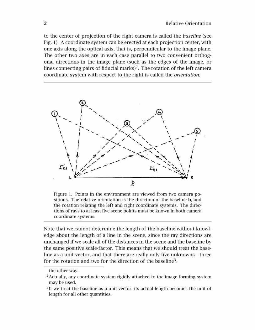
to the center of projection of the right camera is called the baseline (seeFig. 1). A coordinate system can be erected at each projection center, withone axis along the optical axis, that is, perpendicular to the image plane.The other two axes are in each case parallel to two convenient orthog-onal directions in the image plane (such as the edges of the image, orlines connecting pairs of fiducial marks)2. The rotation of the left cameracoordinate system with respect to the right is called the orientation.
Figure 1. Points in the environment are viewed from two camera po-sitions. The relative orientation is the direction of the baseline b, andthe rotation relating the left and right coordinate systems. The direc-tions of rays to at least five scene points must be known in both cameracoordinate systems.
Note that we cannot determine the length of the baseline without knowl-edge about the length of a line in the scene, since the ray directions areunchanged if we scale all of the distances in the scene and the baseline bythe same positive scale-factor. This means that we should treat the base-line as a unit vector, and that there are really only five unknowns—threefor the rotation and two for the direction of the baseline3.
the other way.2Actually, any coordinate system rigidly attached to the image forming systemmay be used.
3If we treat the baseline as a unit vector, its actual length becomes the unit oflength for all other quantities.

2. Existing Solution Methods 3
2. Existing Solution Methods
Various empirical procedures have been devised for determining the rela-tive orientation in an analog fashion. Most commonly used are stereoplot-ters, optical devices that permit viewing of image pairs and superimposedsynthetic features called floating marks. Differences in ray direction par-allel to the baseline are called horizontal disparities (orx-parallaxes), whiledifferences in ray direction orthogonal to the baseline are called verticaldisparities (or y-parallaxes)4. Horizontal disparities encode distances topoints on the surface and are the quantities sought after in measurementof the underlying topography. There should be no vertical disparitieswhen the device is adjusted to the correct relative orientation, since therays from the left and right projection center must lie in a plane thatcontains the baseline (an epipolar plane) if they are to intersect.
The methods used in practice to determine the correct relative ori-entation depend on successive adjustments to eliminate the vertical dis-parity at each of five or six image points that are arranged in one or an-other specially designed pattern [Sailor 60] [Thompson 64] [Slama et al. 80][Moffit & Mikhail 80] and [Wolf 74]. In each of these adjustments, a sin-gle parameter of the relative orientation is varied in order to remove thevertical disparity at one of the points. Which adjustment is made to elim-inate the vertical disparity at a specific point depends on the particularmethod chosen. In each case, however, one of the adjustments, ratherthan being guided visually, is made by an amount that is calculated, usingthe measured values of earlier adjustments. The calculation is based onthe assumptions that the surface being viewed can be approximated bya plane, that the baseline is roughly parallel to this plane, and that theoptical axes of the two cameras are roughly perpendicular to this plane5.
The whole process is iterative in nature, since the reduction of verticaldisparity at one point by means of an adjustment of a single parameter ofthe relative orientation disturbs the vertical disparity at the other points.Convergence is usually rapid if a good initial guess is available. It can beslow, however, when the assumptions on which the calculation is basedare violated, such as in “accidented” or hilly terrain [Van Der Weele 59–60].These methods typically use Euler angles to represent three-dimensional
4This naming convention stems from the observation that, in the usual viewingarrangement, horizontal disparities correspond to left-right displacements inthe image, whereas vertical disparities correspond to up-down displacements.
5While these very restrictive assumptions are reasonable in the case of typicalaerial photography, they are generally not reasonable in the case of terrestrialor industrial photogrammetry, or in robotics.

4 Relative Orientation
rotations [Korn & Korn 68] (traditionally denoted by the greek letters κ,φ, and ω). Euler angles have a number of shortcomings for describingrotations that become particularly noticeable when these angles becomelarge6.
There also exist related digital procedures that converge rapidly whena good initial guess of the relative orientation is available, as is usually thecase when one is interpreting aerial photography [Slama et al. 80]. Not allof these methods use Euler angles. Thompson [1959b], for example, usestwice the Gibb’s vector [Korn & Korn 68] to represent rotations. Theseprocedures may fail to converge to the correct solution when the initialguess is far off the mark. In the application to motion vision, approx-imate translational and rotational components of the motion are oftennot known initially, so a procedure that depends on good initial guessesis not particularly useful. Also, in terrestrial, close-range [Okamoto 81]and industrial photogrammetry [Fraser & Brown 86] good initial guessesare typically harder to come by than they are in aerial photography.
Normally, the directions of the rays are obtained from points gener-ated by projection onto a planar imaging surface. In this case the direc-tions are confined to the field of view as determined by the active area ofthe image plane and its distance to the center of projection. The field ofview is always less than a hemisphere, since only points in front of thecamera can be imaged7. The method described here applies, however, nomatter how the directions to points in the scene are determined. Thereis no restriction on the possible ray directions. We do assume, however,that we can tell which of two opposite semi-infinite line-segments thepoint lies on. If a point lies on the correct line-segment we will say thatit lies in front of the camera, otherwise it will be considered to be behindthe camera (even when these terms do not strictly apply).
The problem of relative orientation is generally considered solved,and so has received little attention in the photogrammetric literature inrecent times [Van Der Weele 59–60]. In the annual index of Photogrammet-ric Engineering, for example, there is only one reference to the subject inthe last ten years [Ghilani 83] and six in the decade before that. This is verylittle in comparison to the large number of papers on this subject in thefifties, as well as the sixties, including [Gill 64] [Sailor 65] [Jochmann 65][Ghosh 66] [Forrest 66] and [Oswal 67].
In this paper we discuss the relationship of relative orientation to the
6The angles tend to be small in traditional applications to photographs takenfrom the air, but often are quite large in the case of terrestrial photogrammetry.
7The field of view is, however, larger than a hemisphere in some fish-eye lenses,where there is significant radial distortion.

3. Coplanarity Condition 5
problem of motion vision in the situation where the motion between theexposure of successive frames is relatively large. Also, a new iterative al-gorithm is described, as well as a way of dealing with the situation whenthere is no initial guess available for the rotation or the direction of thebaseline. The advantages of the unit quaternion notation for represent-ing rotations are illustrated as well. Finally, we discuss critical surfaces,surface shapes that lead to difficulties in establishing a unique relativeorientation.
(One of the reviewers pointed out that L. Hinsken recently obtained amethod for computing the relative orientation based on a parameteriza-tion of the rotation matrix that is similar to the unit quaternion represen-tation used here [Hinsken 87, 88]. In his work, the unknown parametersare the rotations of the left and right cameras with respect to a coordinatesystem fixed to the baseline, while here the unknowns are the directionof the baseline and the rotation of a coordinate system fixed to one of thecameras in a coordinate system fixed to the other camera. Hinsken alsoaddresses the simultaneously orientation of more than two bundles ofrays, but says little about multiple solutions, critical surfaces, and meth-ods for searching the space of unknown parameters.)
3. Coplanarity Condition
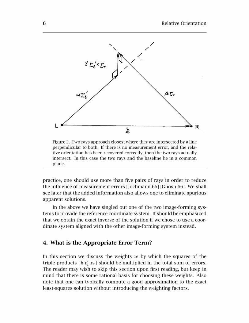
If the ray from the left camera and the corresponding ray from the rightcamera are to intersect, they must to lie in a plane that also contains thebaseline. Thus, if b is the vector representing the baseline, rr the ray fromthe right projection center to the point in the scene and rl the ray fromthe left projection center to the point in the scene, then the triple product
[b r′l rr ] (1)equals zero, where r′l = Rot(rl) is the left ray rotated into the right cam-era’s coordinate system8. This is the coplanarity condition (see Fig. 2).
We obtain one such constraint from each pair of rays. There will bean infinite number of solutions for the baseline and the rotation whenthere are fewer than five pairs of rays, since there are five unknowns andeach pair of rays yields only one constraint. Conversely, if there are morethan five pairs of rays, the constraints are likely to be inconsistent as theresult of small errors in the measurements. In this case, no exact solutionof the set of constraint equations will exist, and it makes sense insteadto minimize the sum of squares of errors in the constraint equations. In
8The baseline vector b is here also assumed to be measured in the coordinatesystem of the right camera.
6 Relative Orientation
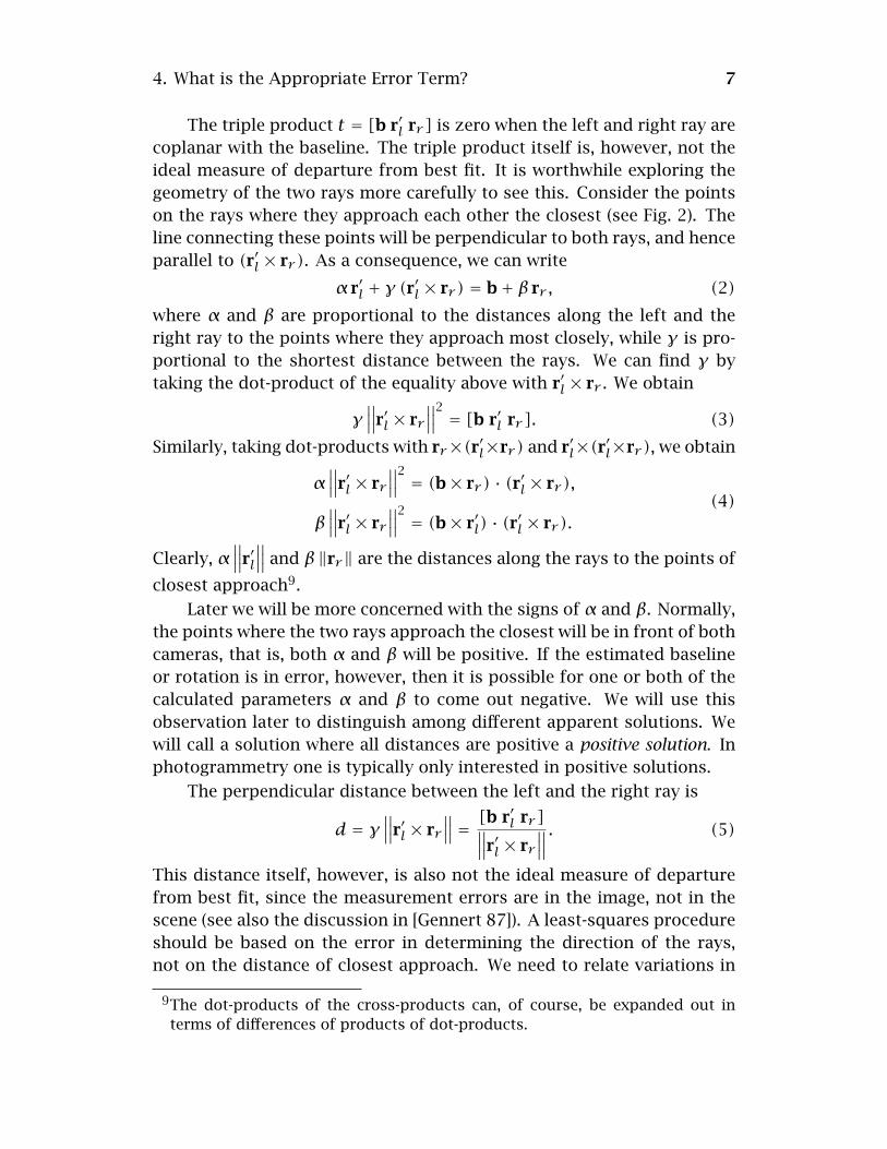
Figure 2. Two rays approach closest where they are intersected by a lineperpendicular to both. If there is no measurement error, and the rela-tive orientation has been recovered correctly, then the two rays actuallyintersect. In this case the two rays and the baseline lie in a commonplane.
practice, one should use more than five pairs of rays in order to reducethe influence of measurement errors [Jochmann 65] [Ghosh 66]. We shallsee later that the added information also allows one to eliminate spuriousapparent solutions.
In the above we have singled out one of the two image-forming sys-tems to provide the reference coordinate system. It should be emphasizedthat we obtain the exact inverse of the solution if we chose to use a coor-dinate system aligned with the other image-forming system instead.
4. What is the Appropriate Error Term?
In this section we discuss the weights w by which the squares of thetriple products [b r′l rr ] should be multiplied in the total sum of errors.The reader may wish to skip this section upon first reading, but keep inmind that there is some rational basis for choosing these weights. Alsonote that one can typically compute a good approximation to the exactleast-squares solution without introducing the weighting factors.
4. What is the Appropriate Error Term? 7
The triple product t = [b r′l rr ] is zero when the left and right ray arecoplanar with the baseline. The triple product itself is, however, not theideal measure of departure from best fit. It is worthwhile exploring thegeometry of the two rays more carefully to see this. Consider the pointson the rays where they approach each other the closest (see Fig. 2). Theline connecting these points will be perpendicular to both rays, and henceparallel to (r′l × rr ). As a consequence, we can write
α r′l + γ (r′l × rr ) = b+ β rr , (2)where α and β are proportional to the distances along the left and theright ray to the points where they approach most closely, while γ is pro-portional to the shortest distance between the rays. We can find γ bytaking the dot-product of the equality above with r′l × rr . We obtain
γ∥∥∥r′l × rr
∥∥∥2 = [b r′l rr ]. (3)Similarly, taking dot-products with rr×(r′l×rr ) and r′l×(r′l×rr ), we obtain
α∥∥∥r′l × rr
∥∥∥2 = (b× rr ) · (r′l × rr ),
β∥∥∥r′l × rr
∥∥∥2 = (b× r′l) · (r′l × rr ).(4)
Clearly, α∥∥∥r′l∥∥∥ and β‖rr‖ are the distances along the rays to the points of
closest approach9.
Later we will be more concerned with the signs of α and β. Normally,the points where the two rays approach the closest will be in front of bothcameras, that is, both α and β will be positive. If the estimated baselineor rotation is in error, however, then it is possible for one or both of thecalculated parameters α and β to come out negative. We will use thisobservation later to distinguish among different apparent solutions. Wewill call a solution where all distances are positive a positive solution. Inphotogrammetry one is typically only interested in positive solutions.
The perpendicular distance between the left and the right ray is
d = γ∥∥∥r′l × rr
∥∥∥ = [b r′l rr ]∥∥∥r′l × rr∥∥∥ . (5)
This distance itself, however, is also not the ideal measure of departurefrom best fit, since the measurement errors are in the image, not in thescene (see also the discussion in [Gennert 87]). A least-squares procedureshould be based on the error in determining the direction of the rays,not on the distance of closest approach. We need to relate variations in
9The dot-products of the cross-products can, of course, be expanded out interms of differences of products of dot-products.

8 Relative Orientation
ray direction to variations in the perpendicular distance between the rays,and hence the triple product.
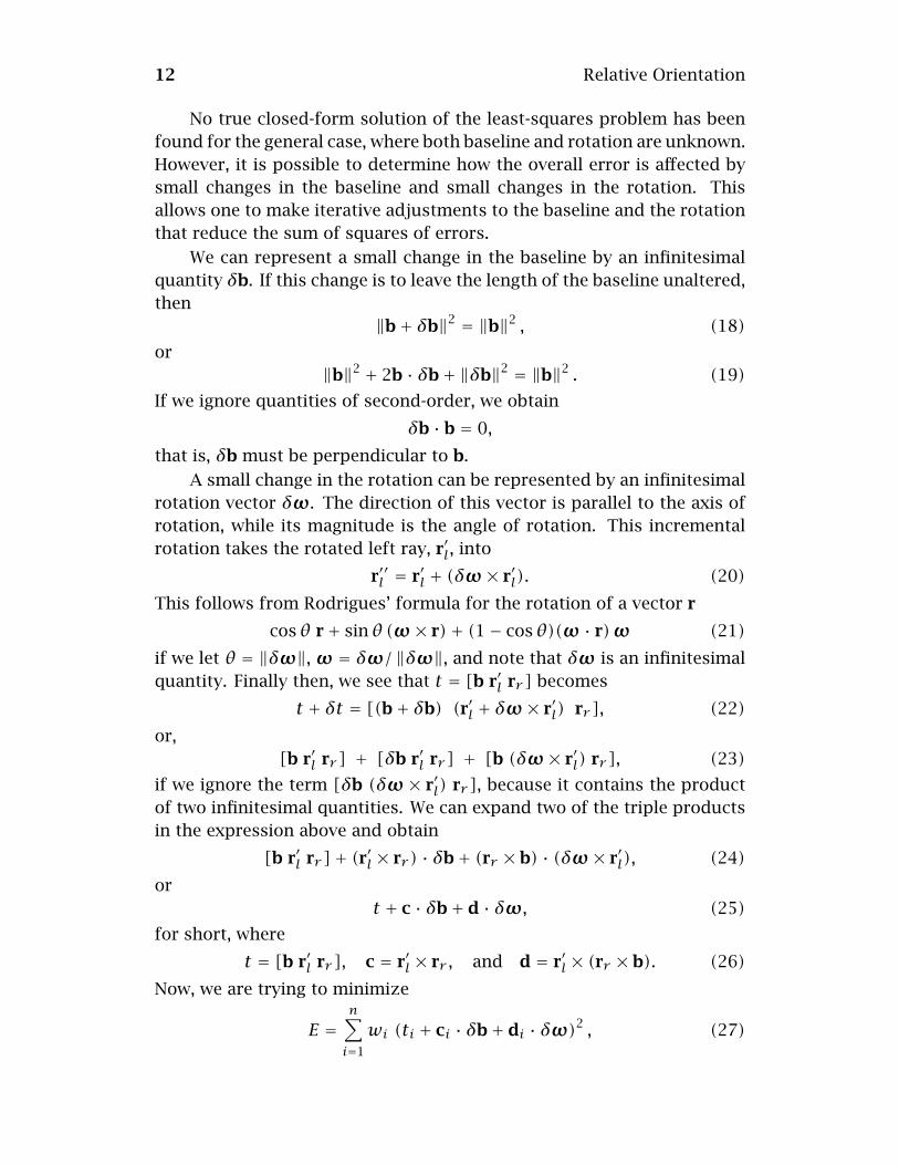
Suppose that there is a change δθl in the vertical disparity of the leftray direction and δθr in the vertical disparity of the right ray direction.That is, r′l and rr are changed by adding
δr′l =r′l × rr∥∥∥r′l × rr
∥∥∥∥∥∥r′l∥∥∥δθl and δrr = r′l × rr∥∥∥r′l × rr
∥∥∥ ‖rr‖δθr , (6)
respectively. Then, from Fig. 3, we see that the change in the perpendic-ular distance d is just δθl times the distance form the left center of pro-jection to the point of closest approach on the left ray, minus δθr timesthe distance from the right center of projection to the point of closestapproach on the right ray, or
δd = α∥∥∥r′l∥∥∥δθl − β‖rr‖δθr . (7)
From equation (5) we see that the corresponding change in the triple prod-uct is
δt =∥∥∥r′l × rr
∥∥∥ δd.Thus if the variance in the determination of the vertical disparity of the leftray is σ 2
l , and the variance in the determination of the vertical disparityof the right ray is σ 2
r , then the variance in the triple product will be10
σ 2t =
∥∥∥r′l × rr∥∥∥2σ 2d, (8)
or
σ 2t =
∥∥∥r′l × rr∥∥∥2(α2∥∥∥r′l∥∥∥2σ 2l + β2 ‖rr‖2 σ 2
r
). (9)
This implies that we should apply a weight
w = σ 20 /σ
2t (10)
to the square of each triple product in the sum to be minimized, whereσ 2
0 is arbitrary (see page 65 in [Mikhail & Ackerman 76]). Written out infull we have
w =∥∥∥r′l × rr
∥∥∥2σ 2
0((b× rr ) · (r′l × rr )
)2∥∥∥r′l∥∥∥2σ 2l +
((b× r′l) · (r′l × rr )
)2 ‖rr‖2 σ 2r
.
(11)
10The error in determining the direction of a ray depends on image position,since a fixed interval in the image corresponds to a larger angular interval inthe middle of the image than it does at the periphery. The reason is that themiddle of the image is closer to the center of projection than is the periphery. Inany case, one can determine what the variance of the error in vertical disparityis, given the image position and the estimated error in determining positionsin the image.
5. Least Squares Solution for the Baseline 9
(Note again that errors in the horizontal disparity do not influence thecomputed relative orientation; instead influencing errors in the distancesrecovered using the relative orientation).
Introduction of the weighting factors makes the sum to be minimizedquite complicated, since changes in baseline and rotation affect both nu-merators and denominators of the terms in the total error sum. Nearthe correct solution, the triple products will be small and so changes inthe estimated rotation and baseline will tend to induce changes in thetriple products that are relatively large compared to the magnitudes ofthe triple products themselves. The changes in the weights, on the otherhand, will generally be small compared to the weights themselves. Thissuggests that one should be able to treat the weights as constant duringa particular iterative step.
Also note that one can compute a good approximation to the solutionwithout introducing the weighting factors at all. This approximation canthen be used to start an iterative procedure that does take the weightsinto account, but treats them as constant during each iterative step. Thisworks well because changes in the weights become relatively small as thesolution is approached.
5. Least Squares Solution for the Baseline
If the rotation is known, it is easy to find the best fit baseline, as we shownext. This is useful, despite the fact that we do not usually know therotation. The reason is that the ability to find the best baseline, givena rotation, reduces the dimensionality of the search space from five tothree. This makes it much easier to systematically explore the space ofpossible starting values for the iterative algorithm.
Let {rl,i} and {rr ,i}, for i = 1 . . . n, be corresponding bundles of leftand right rays. We wish to minimize
E =n∑i=1
wi [b r′l,i rr ,i]2 =n∑i=1
wi(b · (r′l,i × rr ,i)
)2, (12)
subject to the condition b · b = 1, where r′l,i is the rotated left ray rl,i, asbefore. If we let ci = r′l,i× rr ,i, we can rewrite the sum in the simpler form
E =n∑i=1
wi (b · ci)2 = bT
⎛⎝ n∑i=1
wi cicTi
⎞⎠b, (13)
where we have used the equivalence b · ci = bTci, which depends on theinterpretation of column vectors as 3 × 1 matrices. The term cic
Ti is a

10 Relative Orientation
Figure 3. Variations in the triple product t = [b r′l rr ] can be related tovariations in the perpendicular distance d between the two rays. Vari-ations in this distance, in turn, can be related to variations in the mea-surement of the directions of the left and right rays. These relationshipscan be used to arrive at weighting factors that allow minimization of er-rors in image positions while working with the sums of squares of tripleproducts.
dyadic product, a 3× 3 matrix obtained by multiplying a 3× 1 matrix bya 1× 3 matrix.
The error sum is a quadratic form involving the real symmetric ma-trix11.
C =n∑i=1
wi cicTi . (14)
The minimum of such a quadratic form is the smallest eigenvalue of thematrix C , attained when b is the corresponding unit eigenvector (see, forexample, the discussion of Rayleigh’s quotient in [Korn & Korn 68]). Thiscan be verified by introducing a Lagrangian multiplier λ and minimizing
E′ = bTC b+ λ(1− bTb), (15)subject to the condition bTb = 1. Differentiating with respect to b and
11The terms in the sum of dyadic products forming the matrix C contain theweights discussed in the previous section. This only makes sense, however, if aguess is already available for the baseline—unit weights may be used otherwise.
6. Iterative Improvement of Relative Orientation. 11
setting the result equal to zero yields
C b = λb. (16)The error corresponding to a particular solution of this equation is foundby premultiplying by bT :
E = bTC b = λbTb = λ. (17)The three eigenvalues of the real symmetric matrix C are non-negative,and can be found in closed form by solving a cubic equation, while eachof the corresponding eigenvectors has components that are the solutionof three homogeneous equations in three unknowns [Korn & Korn 68].If the data are relatively free of measurement error, then the smallesteigenvalue will be much smaller than the other two, and a reasonableapproximation to the sought-after result can be obtained by solving for theeigenvector using the assumption that the smallest eigenvalue is actuallyzero. This way one need not even solve the cubic equation (see also [Horn& Weldon 88]).
If b is a unit eigenvector, so is −b. Changing the sense of the baselinedoes not change the magnitude of the error term [b r′l rr ]. It does, how-ever, change the signs of α, β and γ. One can decide which sense of thebaseline direction is appropriate by determining the signs of αi and βifor i = 1 . . . n. Ideally, they should all be positive, but when the baselineand the rotation are incorrect they may not be.
The solution for the optimal baseline is not unique unless there are atleast two pairs of corresponding rays. The reason is that the eigenvectorwe are looking for is not uniquely determined if more than one of theeigenvalues is zero, and the matrix has rank less than two if it is the sumof fewer than two dyadic products of independent vectors. This is not asignificant restriction, however, since we need at least five pairs of raysto solve for the rotation anyway.
6. Iterative Improvement of Relative Orientation.
If one ignores the orthonormality of the rotation matrix, a set of nine ho-mogeneous linear equations can be obtained by a transformation of thecoplanarity conditions that was first described in [Thompson 59b]. Theseequations can be solved when eight pairs of corresponding ray directionsare known [Rinner 63] [Longuet-Higgins 81]. This is not a least-squaresmethod that can make use of redundant measurements, nor can it be ap-plied when fewer than eight points are given. The method is also stronglyaffected by measurement errors and fails for certain configurations ofpoints [Longuet-Higgins 84].
12 Relative Orientation
No true closed-form solution of the least-squares problem has beenfound for the general case, where both baseline and rotation are unknown.However, it is possible to determine how the overall error is affected bysmall changes in the baseline and small changes in the rotation. Thisallows one to make iterative adjustments to the baseline and the rotationthat reduce the sum of squares of errors.
We can represent a small change in the baseline by an infinitesimalquantity δb. If this change is to leave the length of the baseline unaltered,then
‖b+ δb‖2 = ‖b‖2 , (18)or
‖b‖2 + 2b · δb+ ‖δb‖2 = ‖b‖2 . (19)If we ignore quantities of second-order, we obtain
δb · b = 0,that is, δb must be perpendicular to b.
A small change in the rotation can be represented by an infinitesimalrotation vector δωω. The direction of this vector is parallel to the axis ofrotation, while its magnitude is the angle of rotation. This incrementalrotation takes the rotated left ray, r′l, into
r′′l = r′l + (δωω× r′l). (20)This follows from Rodrigues’ formula for the rotation of a vector r
cosθ r+ sinθ (ωω× r)+ (1− cosθ)(ωω · r)ωω (21)if we let θ = ‖δωω‖, ωω = δωω/‖δωω‖, and note that δωω is an infinitesimalquantity. Finally then, we see that t = [b r′l rr ] becomes
t + δt = [(b+ δb) (r′l + δωω× r′l) rr ], (22)or,
[b r′l rr ] + [δb r′l rr ] + [b (δωω× r′l) rr ], (23)if we ignore the term [δb (δωω × r′l) rr ], because it contains the productof two infinitesimal quantities. We can expand two of the triple productsin the expression above and obtain
[b r′l rr ]+ (r′l × rr ) · δb+ (rr × b) · (δωω× r′l), (24)or
t + c · δb+ d · δωω, (25)for short, where
t = [b r′l rr ], c = r′l × rr , and d = r′l × (rr × b). (26)Now, we are trying to minimize
E =n∑i=1
wi (ti + ci · δb+ di · δωω)2 , (27)
6. Iterative Improvement of Relative Orientation. 13
subject to the condition b·δb = 0. We can introduce a Lagrange multiplierin order to deal with the constraint. Instead of minimizing E itself, we thenhave to minimize:
E′ = E + 2λ(b · δb), (28)(where the factor of two is introduced to simplify the algebra later). Dif-ferentiating E′ with respect to δb, and setting the result equal to zeroyields
n∑i=1
wi (ti + ci · δb+ di · δωω) ci + λb = 0. (29)
By taking the dot-product of this expression with b, and using the factthat b · b = 1 one can see that
λ = −n∑i=1
wi ti (ti + ci · δb+ di · δωω) , (30)
which means that −λ is equal to the total error when one is at a stationarypoints, where δb and δωω are equal to zero.
If we differentiate E′ with respect to δωω and set this result also equalto zero, we obtain
n∑i=1
wi (ti + ci · δb+ di · δωω)di = 0. (31)
Finally, if we differentiate E′ with respect to λ we get back the constraint
b · δb = 0. (32)The two vector equations and the one scalar equation (equations (29),(31) & (32)) constitute seven linear scalar equations in the six unknowncomponents of δb and δωω and the unknown Lagrangian multiplier λ. Wecan rewrite them in the more compact form:
C δb + F δωω + λb = −c
FT δb+Dδωω = −d
bT δb = 0
(33)
or ⎛⎜⎝C F bFT D 0bT 0T 0
⎞⎟⎠⎛⎜⎝δbδωωλ
⎞⎟⎠ = −
⎛⎜⎝
cd0
⎞⎟⎠ (34)
where
C =n∑i=1
wi cicTi , F =n∑i=1
wi cidTi , and D =n∑i=1
wi didTi , (35)
while
c =n∑i=1
wi ti ci and d =n∑i=1
wi ti di. (36)

14 Relative Orientation
The above gives us a way of finding small changes in the baseline androtation that reduce the overall error sum12. The equations shown (equa-tion (34)) are the symmetric normal equations (see also page 229 in [Mikhail& Ackerman 76]) and yield incremental adjustments for the rotation andthe baseline13. This method can be applied iteratively to locate a mini-mum. Numerical experiments confirm that it converges rapidly when agood initial guess is available.
7. Singularities and Sensitivity to Errors
The computation of the incremental adjustments cannot be carried outwith precision when the coefficient matrix becomes ill-conditioned. Thisoccurs when there are fewer than five pairs of rays, as well as for certainrare configurations of points in the scene (see the discussion of critical sur-faces later). The coefficient matrix may also become ill-conditioned whenthe iterative process approaches a stationary point that is not a minimum,as is often found between two nearby local minima. At such points thetotal error will typically still be quite large, yet vary rather slowly overa significant region of parameter space. In this situation the correctionterms δb and δωω that are computed may become very large. Since thewhole method is based on the assumption that these adjustements aresmall, it is important to limit their magnitude14.
To guard against bad data points (and local minima of the error func-tion) it is important to compute the total error before accepting a solution.It should be compared against what is expected, given the variance of theerror in the vertical disparity of the ray directions. The estimate σ̂ 2
0 of thevariance factor σ 2
0 can be obtained from the weighted error sum
E =n∑i=1
wi [b r′l,i rr ,i]2 (37)
12It is also possible to reduce the problem to the solution of six linear equationsin six unknowns by first eliminating the Lagrangian multiplier λ using b ·b = 1[Horn 87c], but this leads to an asymmetrical coefficient matrix that requiresmore work to set up. One of the reviewers pointed out that the symmetricnormal equations can be solved directly, as shown above.
13Note that the customary savings of about half the computation when solving asystem of equations with symmetric coefficient matrix cannot be fully achievedhere since the last element on the main diagonal is zero. It may also be ofinterest to note that the top left 6× 6 submatrix has at most rank n, since it isthe sum of n dyadic products—it thus happens to be singular when n = 5.
14The exact size of the limit is not very important, a limit between 1/10 and 1 onthe combined magnitudes of δb and δωω appears to work quite well.

8. Adjusting the Baseline and the Rotation 15
using the updated values of the rotation and the baseline, or from theapproximation
E =n∑i=1
wi (ti + ci · δb+ di · δωω)2 , (38)
using the computed increments δb and δωω, and the old values of therotation and the baseline. We have
σ̂ 20 = E/(n− 5), (39)
where n is the number of pairs of rays (see also page 115 in [Mikhail &Ackerman 76]). A χ2-test with five degrees of freedom can be applied toσ̂ 2
0 /σ20 to test whether the estimated variance factor deviates significantly
from the assumed value.
The inverse of the normal matrix introduced above has great signifi-cance, since from it can be derived the covariance matrix for the unknownorientation parameters (the elements of δb and δωω) using the covariancematrix of the quantities (c and d) appearing on the right hand side of thenormal equations (see also page 230 [Mikhail & Ackerman 76]). It is im-portant to point out, however, that the variances of the six parametersdo not tell the whole story, since the covariances (off-diagonal elements)can become very large, particularly in ill-conditioned cases. In such cases,the total error may vary appreciable when any one of the parameters ischanged individually, yet a carefully chosen combination of changes inthe parameters may leave the total error almost unchanged. In these sit-uations, movement along special directions in parameter space may yieldchanges in total error that are a million-fold smaller than changes inducedby movement in other directions. This means that for the same change inthe total error, movement in parameter space in these special directionscan be a thousand-fold larger than in other directions.
Ideally, a sensitivity analysis should be performed to check the sta-bility of the solution [Förstner 87].
8. Adjusting the Baseline and the Rotation
The iterative adjustment of the baseline is straightforward:
bn+1 = bn + δbn, (40)
where bn is the baseline estimate at the beginning of the n-th iteration,while δbn is the adjustment computed during the n-th iteration, as dis-cussed in the previous section. If δbn is not infinitesimal, the result willnot be a unit vector. We can, and should, normalize the result by dividingby its magnitude.
16 Relative Orientation
8.1 Adjustment of Rotation using Unit Quaternions
Adjusting the rotation is a little harder. Rotations are conveniently rep-resented by unit quaternions [Stuelpnagle 64] [Salamin 79] [Taylor 82][Horn 86, 87a]. The groundwork for the application of the unit quater-nion notation in photogrammetry was laid by Thompson [1959a], Schut[1958–59] and Pope [1970]. A positive rotation about the axis ωω throughan angle θ is represented by the unit quaternion
q̊ = cos(θ/2)+ sin(θ/2) ωω, (41)
where ωω is assumed to be a unit vector. Composition of rotations cor-responds to multiplication of the corresponding unit quaternions. Therotated version of a vector r is computed using
r̊′ = q̊ r̊ q̊∗, (42)
where q̊∗ is the conjugate of the quaternion q̊, that is, the quaternion ob-tained by changing the sign of the vector part. Here, r̊ is a purely imaginaryquaternion with vector part r, while r̊′ is a purely imaginary quaternionwith vector part r′. The above can also be written in the form
r′ = (q20 − q · q) r+ 2(q · r)q+ 2q0(q× r), (43)
where q0 and q are the scalar and vector parts of the unit quaternion q̊(see also [Horn 86]).
The infinitesimal rotation δωω corresponds to the quaternion
δω̊ = 1+ 12δωω. (44)
We can adjust the rotation q̊ by premultiplying with δω̊, that is,
q̊n+1 = δω̊n q̊n. (45)
If δωωn is not infinitesimal, δω̊n will not be a unit quaternion, and sothe result of the adjustment will not be a unit quaternion either. Thisundesirable state of affairs can be avoided by using either of the two unitquaternions
δω̊ =√
1− 14‖δωω‖2 + 1
2δωω, (46)
or
δω̊ =(1+ 1
2δωω
)/√1+ 1
4‖δωω‖2 . (47)
Alternatively, one can simply normalize the product by dividing by itsmagnitude.

8. Adjusting the Baseline and the Rotation 17
8.2 Adjustment of Rotation using Orthonormal Matrices
The adjustment of rotation is a little trickier if orthonormal matrices areused to represent rotations. We can write the relationship
r′ = r+ (δωω× r), (48)in the form
r′ = r+W r, (49)where the skew-symmetric matrix W is defined by
W =⎛⎜⎝
0 −δωωz δωωy
δωωz 0 −δωωx
−δωωy δωωx 0
⎞⎟⎠ , (50)
in terms of the components of rotation vector δωω = (δωωx,δωωy,δωωz)T .Consequently we may write r′ = Q r, where Q = I +W , or
Q =⎛⎜⎝
1 −δωωz δωωy
δωωz 1 −δωωx
−δωωy δωωx 1
⎞⎟⎠ , (51)
One could then attempt to adjust the rotation by multiplication of thematrices Q and R as follows:
Rn+1 = QnRn. (52)The problem is that Q is not orthonormal unless δωω is infinitesimal. Inpractice this means that the rotation matrix will depart more and morefrom orthonormality as more and more iterative adjustments are made. Itis possible to re-normalize this matrix by finding the nearest orthonormalmatrix, but this is complicated, involving the determination of the square-root of a symmetric matrix [Horn et al. 88]15.
To avoid this problem, we should really start with an orthonormalmatrix to represent the incremental rotation. We can use either of the twounit quaternions in equations (46) or (47) to construct the correspondingorthonormal matrix
Q =⎛⎜⎝q2
0 + q2x − q2
y − q2z 2(qxqy − q0qz) 2(qxqz + q0qy)
2(qyqx + q0qz) q20 − q2
x + q2y − q2
z 2(qyqz − q0qx)2(qzqx − q0qy) 2(qzqy + q0qx) q2
0 − q2x − q2
y + q2z
⎞⎟⎠ ,(53)
where q0 is the scalar part of the quaternion δω̊, while qx , qy , qz arethe components of the vector part.16 Then the adjustment of rotation is
15This is another place where the unit quaternion representation has a distinctadvantage: it is trivial to find the nearest unit quaternion to a quaternion thatdoes not have unit magnitude.
16This expression for the orthonormal normal matrix in terms of the componentsof the corresponding unit quaternion can be obtained directly by expandingr̊′ = q̊ r̊ q̊∗ or by means of Rodrigues’ formula [Horn 86, 87a].
18 Relative Orientation
accomplished usingRn+1 = QnRn. (54)
Note, however, that the resulting matrices will still tend to depart slightlyfrom orthonormality due to numerical inaccuracies. This may be a prob-lem if many iterations are required.
9. Ambiguities
9.1 Inherent Ambiguities and Dual Solution
The iterative adjustment described above may arrive at a number of appar-ently different solutions. Some of these are just different representationsof the same solution, while others are related to the correct solution bya simple transformation. First of all, note that −q̊ represents the samerotation as q̊, since
(−q̊) r̊ (−q̊∗) = q̊ r̊ q̊∗. (55)That is, antipodal points on the unit sphere in four dimensions representthe same rotation. If desired, one can prevent any confusion by ensur-ing that the first nonzero component of the resulting unit quaternion ispositive, or that the largest component is positive.
Next, note that the triple product, [b r′l rr ], changes sign, but notmagnitude, when we replace b with −b. Thus the two possible senses ofthe baseline yield the same sum of squares of errors. However, changingthe sign of b does change the signs of both α and β. All scene pointsimaged are in front of the camera, so the distances should all be positive.In the presence of noise, it is possible that some of the distances turnout to be negative, but with reasonable data almost all of them shouldbe positive. This normally allows one to pick the correct sense for thebaseline.
Not so obvious is another possibility: Suppose we turn all of the leftmeasurements through π radians about the baseline, in addition to therotation already determined. That is, replace q̊ by q̊′ = b̊ q̊, where b̊ is apurely imaginary quaternion with vector part b. The triple product canbe written in the form
t = [b r′l rr ] = Rot(rl) · (rr × b) = (q̊ r̊l q̊∗) · (̊rr b̊), (56)
where r̊l and r̊r are purely imaginary quaternion with vector part rl and rrrespectively. If we replace q̊ by q̊′ = b̊ q̊, we obtain for the triple product
t′ = (b̊ q̊ r̊l q̊∗ b̊∗) · (̊rr b̊) = (b̊ q̊ r̊l q̊
∗) · (̊rr b̊ b̊), (57)or
t′ = (b̊ q̊ r̊l q̊∗) · (−b · b)̊rr = −(b̊ q̊ r̊l q̊
∗) · r̊r , (58)
9. Ambiguities 19
ort′ = −(q̊ r̊l q̊
∗) · (b̊∗ r̊r ) = −(q̊ r̊l q̊∗) · (̊rr b̊) = −t, (59)
where we have repeatedly used special properties of purely imaginaryquaternions, as well as the fact that b · b = 1. We conclude that the signof the triple product is changed by the added rotation, but its magnitudeis not. Thus the total error is undisturbed when the left rays are rotatedthrough π radians about the baseline. The solution obtained this way willbe called the dual of the other solution.
We can obtain the same result using vector notation: We replace r′lwith
r′′l = 2(b · r′l)b− r′l. (60)using Rodrigues’ formula for the rotation of a vector r
cosθ r+ sinθ (ωω× r)+ (1− cosθ)(ωω · r)ωω, (61)with θ = π and ωω = b. Then the triple product [b r′l rr ] turns into
2(b · r′l)[b b rr ]− [b r′l rr ] = −[b r′l rr ]. (62)This, once again, reverses the sign of the error term, but not its magnitudeThus the sum of squares of errors is unaltered. The signs of α and β areaffected, however, although this time not in as simple a way as when thesense of the baseline was reversed.
If [b r′l rr ] = 0, we find that exactly one of α and β changes sign. Thiscan be shown as follows: The triple product will be zero when the left andright rays are coplanar with the baseline. In this case we have γ = 0, andso
α r′l = b+ β rr , (63)Taking the cross-product with b we obtain
α(r′l × b) = β(rr × b), (64)If we now replace r′l by r′′l = 2(b · r′l)b− r′l, we have for the new distancesα′ and β′ along the rays:
−α′ (r′l × b) = β′ (rr × b), (65)We conclude that the productα′β′ has sign opposite to that of the productαβ. So if α and β are both positive, one of α′ or β′ must be negative.
In the presence of measurement error the triple product will not beexactly equal to zero. If the rays are nearly coplanar with the baseline,however, we find that one of α and β almost always changes sign. Withvery poor data, it is possible that both change sign17. In any case, we canreject a solution in which roughly half the distances are negative. More-over, we can find the correct solution directly by introducing an additional
17Even with totally random ray directions, however, this only happens 27.3% ofthe time, as determined by Monte Carlo simulation.
20 Relative Orientation
rotation of π radians about the baseline, that is, by computing the dualof the solution.
9.2 Remaining Ambiguity
If we take care of the three apparent two-way ambiguities discussed inthe previous section, we find that in practice a unique solution is found,provided that a sufficiently large number of ray pairs are available. That is,the method converges to the unique global minimum from every possiblystarting point in parameter space18.
Several local minima in the sum of squares of errors appear whenonly a few more than the minimum of five ray pairs are available (as iscommon in practice). This means that one has to repeat the iteration withdifferent starting values for the rotation in order to locate the global min-imum. A starting value for the baseline can be found in each case usingthe closed-form method described in section 5. To search the parame-ter space effectively, one needs a way of efficiently sampling the spaceof rotations. The space of rotations is isomorphic to the unit sphere infour dimensions, with antipodal points identified. The rotation groups ofthe regular polyhedra provide convenient means of uniformly samplingthe space of rotations. The group of rotations of the tetrahedron has 12elements, that of the hexahedron and the octahedron has 24, and that ofthe icosahedron and the dodecahedron has 60 (representations of thesegroups are given in Appendix A for convenience). One can use these asstarting values for the rotation. Alternatively, one can just generate anumber of randomly placed points on the unit sphere in four dimensionsas starting values for the rotation19.
9.3 Number of Solutions Given Five Pairs of Rays
When there are exactly five pairs of rays, the situation is different again. Inthis case, we have five nonlinear equations (equation (1)) in five unknownsand so in general expect to find a finite number of exact solutions. Thatis, it is possible to find baselines and rotations that satisfy the coplanarityconditions exactly and reduce the sum of squares of errors to zero.
18It has been shown that at most three essentially different relative orientationsare compatible with a given sufficiently large number of ray pairs [Longuet-Higgins 88]—in practice one typically finds just one.
19We see here another advantage of the unit quaternion representation. It is notclear how one would sample the space of rotations using orthonormal matricesdirectly.
9. Ambiguities 21
We can in fact easily express the coplanarity constraint as a polyno-mial in the components of b and q̊. Noting that r′l = Rot(rl) and that thetriple product can be written in the form
t = [b r′l rr ] = (q̊ r̊l q̊∗) · (̊rr b̊) (66)
we can expand equation (1), using equation (53), into((q2
0+q2x−q2
y−q2z)lx+2(qxqy−q0qz)ly+2(qxqz+q0qy)lz
)(rybz−rzby)+(
2(qyqx+q0qz)lx+(q20−q2
x+q2y−q2
z)ly+2(qyqz−q0qx)lz)(rzbx−rxbz)+(
2(qzqx−q0qy)lx+2(qzqy+q0qx)ly+(q20−q2
x−q2y+q2
z)lz)(rxby−rybx)= 0 (67)
where b = (bx, by, bz)T , rl = (lx, ly , lz)T , rr = (rx, ry, rz)T , while q̊ =(q0, qx, qy, qz)T . This equation is linear in the components of b andquadratic in the components of q̊. When there are five ray pairs, thereare five such equations. Together with the quadratic equations b · b = 1and q̊ · q̊ = 1, they constitute seven polynomial equations in the sevencomponents of b and q̊. An upper bound on the number of solutions isgiven by the product of the orders of the equations, which is 27 = 128 inthis case20. Note however that the equations are not changed if we changethe sign of either b or q̊. Taking this into account, we see that there canbe at most 32 distinct solutions. Not all of these need be real, of course.
In practice it is found that the number of solutions is typically a mul-tiple of four (if we ignore reversals of q̊ and b). With randomly chosen raydirections, about half of the cases lead to eight solutions, slightly morethan a quarter have four solutions, while slightly less than a quarter havetwelve. Less frequent are cases with sixteen solutions and a very smallnumber of randomly generated test cases lead to twenty solutions, whichappears to be the maximum number possible. Ray bundles for whichthere is no solutions at all are equally rare, but do exist. When one of thesolutions corresponds to a critical surface, then the number of solutionsis not a multiple of four—such cases correspond to places in ray param-eter space that lie on the border between regions in which the number ofsolutions are different multiples of four. In this situation, small changesin the ray directions increase or decrease the number of solutions by two.
It has been brought to my attention, after receiving the commentsof the reviewers, that it has recently been shown that there can be atmost twenty solutions [Faugeras & Maybank 89] of the relative orientationproblem whenn = 5, and that there exist pairs of ray bundles that actually
20The three components of the baseline vector b can be eliminated fairly easily,because the equations are linear and homogeneous in these components. Thisleaves a smaller number of higher order equations in the four components ofq̊.
22 Relative Orientation
lead to twenty solutions [Netravali & et al. 89]21. Typically there is onepositive solution (or none), although several positive solutions may existfor a given set of ray bundles.
The ambiguities discussed above are, of course, of little concern ifa reasonable initial guess is available. Note that methods that apply tothe special case when there are five pairs of rays do not generalize to theleast-squares problem when a larger number of ray pairs are available. Inpractice one should use more than five ray pairs, both to improve accuracyand to have a way of judging how large the errors might be.
10. Summary of the Algorithm
Consider first the case where we have an initial guess for the rotation.We start by finding the best-fit baseline direction using the closed-formmethod described in section 5. We may wish to determine the correctsense of the baseline by choosing the one that makes most of the signsof the distances positive. Then we proceed as follows:
• For each pair of corresponding rays, we compute r′l,i, the left ray di-rection rl,i rotated into the right camera coordinate system, usingthe present guess for the rotation (equations (42), (43) or using equa-tion (53)).
• We then compute the cross-product ci = r′l,i × rr ,i, the double cross-product di = r′l,i × (rr ,i × b) and the triple-product ti = [b r′l,i rr ,i].
• If desired, we then compute the appropriate weighting factor wi asdiscussed in section 4 (equation (11)).
• We accumulate the (weighted) dyadic products wi cicTi , wi cidTi andwi didTi , as well as the (weighted) vectors wi tici and wi tidi. Thetotals of these quantities over all ray pairs give us the matrices C , F ,D and the vectors c and d (equations (35) & (36)).
• We can now solve for the increment in the baseline δb and the in-crement in the rotation δωω using the method derived in section 6(equation (34)).
• We adjust the baseline and the rotation using the methods discussedin section 8 (equations (40), (45) or (53), (54)), and recompute the sumof the squares of the error terms (equation (12)).
21Since dual solutions (obtained by rotating the left ray bundle through π aboutthe baseline) are apparently not counted by these authors, they actually claimthat the maximum number of solutions is ten.

11. Search of Parameter Space and Statistics 23
The new orientation parameters are then used in the next iteration of theabove sequence of steps. As is the case with many iterative procedures,it is important to know when to stop. One could stop after either a fixednumber of iterations or when the error becomes less than some prede-termined threshold. Another approach would be to check on the size ofthe increments in the baseline and the rotation These become smaller andsmaller as the solution is approached, although their absolute size doesnot appear to provide a reliable stopping criterion.
The total error typically becomes small after a few iterations and nolonger decreases at each step, because of limited accuracy in the arith-metic operations. So one could stop the iteration the first time the errorincreases. The total error may, however, also increase when the surfacesof constant error in parameter space are very elongated in certain direc-tions, as happens when the problem is ill-conditioned. In this case a stepin the direction of the local gradient can cause one to skip right acrossthe local “valley floor.” It is thus wise to first check whether smaller stepsin the given direction reduce the total error. The iteration is only stoppedwhen small steps also increase the error.
When the decision has been made to stop the iteration, a check ofthe signs of the distances along the rays is in order. If most of them arenegative, the baseline direction should be reversed. If neither sense of thebaseline direction yields mostly positive distances, one needs to considerthe dual solution (rotation of the left ray bundle through π radians aboutthe baseline b).
It makes sense also to check whether the solution is reasonable orwhether it has perhaps been spoilt by some gross error in the data, suchas incorrect correspondence between rays. When more than five pairs ofrays are available, recomputation of the result using sub-sets obtained byomitting one ray at a time yield useful test results. These computationsdo not take much work, since a good guess for the solution is available ineach case.
It is, of course, also useful to compute the total error E and to es-timate the variance factor, as suggested in section 7. Finally, it may bedesirable to estimate the standard deviations of the error in the six un-known parameters using the inverse of the matrix of coefficients of thesymmetric normal equations, as indicated in section 7.
11. Search of Parameter Space and Statistics
If an initial guess is not available, one proceeds as follows:

24 Relative Orientation
• For each rotation in the chosen group of rotations, perform the aboveiteration to obtain a candidate baseline and rotation.
• Choose the solution that has all positive signs of the distances alongrays and yields the smallest total error.
When there are many pairs of rays, the iterative algorithm will converge tothe global minimum error solution from any initial guess for the rotation.There is no need to sample the space of rotations in this case.
Also, instead of sampling the space of rotations in a systematic wayusing a finite group of rotations, one can generate points randomly dis-tributed on the surface of the unit sphere in four-dimensional space. Thisprovides a simpler means of generating initial guesses, although more ini-tial guesses have to be tried than when a systematic procedure is used,since the space of rotations will not be sampled evenly.
The method as presented minimizes the sum of the squares of theweighted triple products [b r′l rr ]. We assumed that the weighting factorsvary slowly during the iterative process, so that we can to use the currentestimates of the baseline and rotation in computing the weighting factors.That is, when taking derivatives, the weighting factors are treated as con-stants. This is a good approximation when the parameters vary slowly, asthey will when one is close to a minimum.
The method described above can be interpreted as a straight-forwardweighted least-squares optimization, which does not allow estimation ofuncertainty in the parameters. One can also apply more sophisticatedanalyses to this problem, such as best linear unbiased estimation, whichdoes not require any assumptions to be made about the distribution ofthe errors, only that their standard deviations be known. The standarddeviations of the resultant parameters can then be used to evaluate theiruncertainty, although no testing of confidence intervals is possible. Fi-nally, one may apply maximum likelihood estimation of the orientationparameters, where the observation errors are assumed to be distributedin a Gaussian fashion with known standard deviations. This allows one toderive confidence regions for the estimate orientation parameters, whichcan be treated as quantities that contain an error that is distributed inGaussian fashion also.
12. Critical Surfaces
In certain rare cases, relative orientation cannot be accurately recovered,even when there are five or more pairs of rays. Normally, each error termvaries linearly with distance in parameter space from the location of an

12. Critical Surfaces 25
extremum, and so the sum of squares of errors varies quadratically. Thereare situations, however, where the error terms to not vary linearly withdistance, but quadratically or higher order, in certain special directionsin parameter space. In this case, the sum of squares of errors does notvary quadratically with distance from the extremum, but as a functionof the fourth or even higher power of this distance. This makes it verydifficult to accurately locate the extremum. In this case, the total erroris not significantly affected by a change in the rotation, as long as thischange is accompanied by an appropriate corresponding change in thebaseline. It turns out that this problem arises only when the observedscene points lie on certain surfaces called Gefährliche Flächen or criticalsurfaces [Brandenberger 47] [Hofmann 49] [Zeller 52] [Schwidefsky 73].We show next that only points on certain hyperboloids of one sheet andtheir degenerate forms can lead to this kind of problem.
We could try to find a direction of movement in parameter space (δb,δωω) that leaves the total error unaffected (to second order) when given aparticular surface. Instead, we will take the critical direction of motion inthe parameter space as given, and try to find a surface for which the totalerror does not change (to second order).
Let R be a point on the surface, measured in the right camera coordi-nate system. Then
β rr = R and α r′l = b+ R, (68)for some positive α and β. In the absence of measurement errors,
[b r′l rr ] = 1αβ[b (b+ R) R] = 0. (69)
We noted earlier that when we change the baseline and the rotation slightly,the triple product [b r′l rr ] becomes
[(b+ δb) (r′l + δωω× r′l) rr ], (70)or, if we ignore higher-order terms,
[b r′l rr ]+ (r′l × rr ) · δb+ (rr × b) · (δωω× r′l). (71)The problem we are focusing on here arises when this error term is un-changed (to second order) for small movement in some direction in theparameter space. That is when
(r′l × rr ) · δb+ (rr × b) · (δωω× r′l) = 0, (72)for some δb and δωω. Introducing the coordinates of the imaged pointswe obtain:
1αβ
(((b+ R)× R
) · δb+ (R × b) · (δωω× (b+ R))) = 0, (73)
or(R × b) · (δωω× R)+ (R × b) · (δωω× b)+ [b R δb] = 0. (74)
26 Relative Orientation
If we expand the first of the dot-products of the cross-products, we canwrite this equation in the form
(R · b)(δωω · R)− (b · δωω)(R · R)+ L · R = 0, (75)where
L = × b, while = b× δωω+ δb. (76)The expression on the left-hand side contains a part that is quadratic in Rand a part that is linear. The expression is clearly quadratic in X, Y , andZ , the components of the vector R = (X, Y , Z)T . Thus a surface leadingto the kind of problem described above must be a quadric surface [Korn& Korn 68].
Note that there is no constant term in the equation of the surface,so R = 0 satisfies the equation (75). This means that the surface passesthrough the right projection center. It is easy to verify that R = −b satis-fies the equation also, which means that the surface passes through theleft projection center as well. In fact, the whole baseline (and its exten-sions), R = kb, lies in the surface. This means that we must be dealingwith a ruled quadric surface. It can consequently not be an ellipsoid orhyperboloid of two sheets, or one of their degenerate forms. The sur-face must be a hyperboloid of one sheet, or one of its degenerate forms.Additional information about the properties of these surfaces is given inAppendix B, while the degenerate forms are explored in Appendix C (seealso [Negahdaripour 89]).
It should be apparent that this kind of ambiguity is quite rare. Thisis nevertheless an issue of practical importance, since the accuracy of thesolution is reduced if the points lie near some critical surface. A textbookcase of this occurs in aerial photography of a roughly U-shaped valleytaken along a flight line parallel to the axis of the valley from a heightabove the valley floor approximately equal to the width of the valley. Inthis case, the surface can be approximated by a portion of a circular cylin-der with the baseline lying on the cylinder. This means that it is closeto one of the degenerate forms of the hyperboloid of one sheet (see Ap-pendix C).
Note that hyperboloids of one sheet and their degenerate forms areexactly the surfaces that lead to ambiguity in the case of motion vision.The coordinate systems and symbols have been chosen here to make thecorrespondence between the two problems more apparent. The relation-ship between the two situations is nevertheless not quite as transparentas I had thought at first [Horn 87b]:
In the case of the ambiguity of the motion field, we are dealing witha two-way ambiguity arising from infinitesimal displacements in camera

13. Conclusions 27
position and orientation. In the case of relative orientation, on the otherhand, we are dealing with an elongated region in parameter space withinwhich the error varies more slowly than quadratically, arising from imagestaken with cameras that have finite differences in position and orientation.Also note that the symbol δωω stands for a small change in a finite rotationhere, while it refers to a difference in instantaneous rotational velocitiesin the motion vision case.
In practice, the relative orientation problem becomes ill-conditionednear a solution that corresponds to ray-intersections that lie close to acritical surface. In this case the surfaces of constant error in parameterspace become very elongated and the location of the true minimum is notwell defined. In addition, iterative algorithms based on local lineariza-tion tend to require many steps for convergence in this situation. It isimportant to point out that a given pair of bundles of corresponding raysmay lead to poor behavior near one particular solution, yet be perfectlywell-behaved near other solutions. In general these sorts of problems aremore likely to be found when the fields of view of one or both cameras aresmall. It is possible, however, to have ill-conditioned problems with widefields of view. Conversely, a small field of view does not automaticallylead to poor behavior.
Difficulties are also encountered when two local minima are near oneanother, since the surfaces of constant error in this case tend to be elon-gated along the direction in parameter space connecting the two minimaand there is a saddle point somewhere between the two minima. At thesaddle point the normal matrix is likely to be singular.
13. Conclusions
Methods for recovering the relative orientation of two cameras are of im-portance in both binocular stereo and motion vision. A new iterativemethod for finding the relative orientation has been described here. Itcan be used even when there is no initial guess available for the rotationor the baseline. The new method does not use Euler angles to representthe orientation and it does not require that the measured points be ar-ranged in a particular pattern, as some previous methods do.
When there are many pairs of corresponding rays, the iterative methodfinds the global minimum from any starting point in parameter space. Lo-cal minima in the sum of squares of errors occur, however, when there arerelatively few pairs of corresponding rays available. Method for efficientlylocating the global minimum in this case were discussed. When only five

28 Relative Orientation
pairs of corresponding rays are given, several exact solutions of the copla-narity equations can be found. Typically only one of these is a positivesolution, that is, one that yields positive distances to all the points in thescene. This allows one to pick the correct solution even when there is noinitial guess available.
The solution cannot be determined with accuracy when the scenepoints lie on a critical surface.
Acknowledgments
The author thanks W. Eric L. Grimson and Rodney A. Brooks, who madehelpful comments on a draft of this paper, as well as Michael Gennertwho insisted that a least-squares procedure should be based on the er-ror in determining the direction of the rays, not on the distance of theirclosest approach. I would also like to thank Shahriar Negadahripour, whoworked on the application of results developed earlier for critical surfacesin motion vision to the case when the step between successive images isrelatively large. Harpreet Sawhney brought the recent paper by Faugerasand Maybank to my attention, while S. (Kicha) Ganapathy alerted me tothe work of Netravali et al.
Finally, I am very grateful to the anonymous reviewers for point-ing out several relevant references, including [Pope 70] [Hinsken 87, 88][Longuet-Higgins 88] and for making significant contributions to the pre-sentation. In particular, one of the reviewers drew my attention to thefact that one can solve the symmetric normal equations directly, with-out first eliminating the Lagrange multiplier. This not only simplifies thepresentation, but leads to a (small) reduction in computational effort.
References
Bender, L.U. (1967) “Derivation of Parallax Equations,” Photogrammetric Engineer-ing, Vol. 33, No. 10, pp. 1175–1179, October.
Brandenberger, A. (1947) “Fehlertheorie der äusseren Orientierung von Steilauf-nahmen,” Ph.D. Thesis, Eidgenössische Technische Hochschule, Zürich, Switzer-land.
Brou, P. (1983) “Using the Gaussian Image to Find the Orientation of an Object,”International Journal of Robotics Research, Vol. 3, No. 4, pp. 89–125.
Bruss, A.R. & B.K.P. Horn, (1983) “Passive Navigation,” Computer Vision, Graphics,and Image Processing, Vol. 21, No. 1, January, pp. 3–20.
13. Conclusions 29
Faugeras, O.D. & S. Maybank (1989) “Motion from Point Matches: Multiplicity ofSolutions,” Proceedings of IEEE Workshop on Motion Vision, Irvine, CA, March20–22.
Förstner, W. (1987) “Reliability Analysis of Parameter Estimation in Linear Modelswith Applications to Mensuration Problems in Computer Vision,” ComputerVision, Graphics, and Image Processing, Vol. 40, No. 3, pp. 273–310, Decem-ber.
Forrest, R.B. (1966) “AP-C Plotter Orientation,” Photogrammetric Engineering, Vol. 32,No. 5, pp. 1024–1027, September.
Fraser, C.S. & D.C. Brown (1986) “Industrial Photogrammetry: New Developmentsand Recent Applications,” Photogrammetric Record, Vol. 12, No. 68, pp. 197–217, October.
Gennert, Michael A. (1987) “A Computational Framework for Understanding Prob-lems in Stereo Vision,” Ph.D. thesis, Department of Electrical Engineering andComputer Science, MIT, August 1987.
Ghilani, C.D. (1983) “Numerically Assisted Relative Orientation of the Kern PG-2,”Photogrammetric Engineering and Remote Sensing, Vol. 49, No. 10, pp. 1457–1459, October.
Ghosh, S.K. (1966) “Relative Orientation Improvement,” Photogrammetric Engi-neering, Vol. 32, No. 3, pp. 410–414, May.
Ghosh, S.K. (1972) Theory of Stereophotogrammetry, Ohio University Bookstores,Columbus, OH.
Gill, C. (1964) “Relative Orientation of Segmented, Panoramic Grid Models on theAP-II,” Photogrammetric Engineering, Vol. 30, pp. 957–962,
Hallert, B. (1960) Photogrammetry, McGraw-Hill, New York, NY.
Hilbert, D. & S. Cohn-Vossen (1953, 1983) Geometry and the Imagination, ChelseaPublishing, New York.
Hinsken, L. (1987) “Algorithmen zur Beschaffung von Näherungswerten für dieOrientierung von beliebig im Raum angeordneten Strahlenbündeln,” Disser-tation, Deutsche Geodätische Kommision, Reihe C, Heft Nr. 333, München,Federal Republic of Germany.
Hinsken, L. (1988) “A Singularity-Free Algorithm for Spatial Orientation of Bun-dles,” International Archives of Photogrammetry and Remote Sensing, Vol. 27,Part B5, Comm. V, pp. 262–272.
Hofmann, W. (1949) “Das Problem der ‘Gefährlichen Flächen’ in Theorie and Praxis,”Ph.D. Thesis, Technische Hochschule München, Published in 1953 by DeutscheGeodätische Kommission, München, Federal Republic of Germany.
Horn, B.K.P. (1986) Robot Vision, MIT Press, Cambridge, MA & McGraw-Hill, NewYork, NY.
30 Relative Orientation
Horn, B.K.P. (1987a) “Closed-form Solution of Absolute Orientation using UnitQuaternions,” Journal of the Optical Society A, Vol. 4, No. 4, pp. 629–642,April.
Horn, B.K.P. (1987b) “Motion Fields are Hardly Ever Ambiguous,” InternationalJournal of Computer Vision, Vol. 1, No. 3, pp. 263–278, Fall.
Horn, B.K.P. (1987c) “Relative Orientation,” Memo 994, Artificial Intelligence Lab-oratory, MIT, Cambridge, MA. Also, (1988) Proceedings of the Image Under-standing Workshop, 6–8 April, Morgan Kaufman Publishers, San Mateo, CA,pp. 826–837.
Horn, B.K.P., H.M. Hilden & S. Negahdaripour (1988) “Closed-form Solution of Ab-solute Orientation using Orthonormal Matrices,” Journal of the Optical Soci-ety A, Vol. 5, No. 7, pp. 1127–1135, July.
Horn, B.K.P. & E.J. Weldon Jr. (1988) “Direct Methods for Recovering Motion,” In-ternational Journal of Computer Vision, Vol. 2, No. 1, pp. 51–76, June.
Jochmann, H. (1965) “Number of Orientation Points,” Photogrammetric Engineer-ing, Vol. 31. No. 4, pp. 670–679, July.
Korn, G.A. & T.M. Korn (1968) Mathematical Handbook for Scientists and Engineers,2-nd edition, McGraw-Hill, New York, NY.
Longuet-Higgins, H.C. (1981) “A Computer Algorithm for Reconstructing a Scenefrom Two Projections,” Nature, Vol. 293, pp. 133–135, September.
Longuet-Higgins, H.C. (1984) “The Reconstruction of a Scene from Two Projections—Configurations that Defeat the Eight-Point Algorithm,” IEEE, Proceedings ofthe First Conference on Artificial Intelligence Applications, Denver, Colorado.
Longuet-Higgins, H.C. (1988) “Multiple Interpretations of a Pair of Images of aSurface,” Proceedings of the Royal Society of London A, Vol. 418, pp. 1–15.
Longuet-Higgins, H.C. & K. Prazdny (1980) “The Interpretation of a Moving RetinalImage,” Proceedings of the Royal Society of London B, Vol. 208, pp. 385–397.
Mikhail, E.M. & F. Ackerman (1976) Observations and Least Squares, Harper & Row,New York, NY.
Moffit, F. & E.M. Mikhail (1980) Photogrammetry, 3-rd edition, Harper & Row, NewYork, NY.
Negahdaripour, S. (1989) “Multiple Interpretation of the Shape and Motion of Ob-jects from Two Perspective Images,” unpublished manuscript of the WaikikiSurfing and Computer Vision Society of the Department of Electrical Engi-neering at the University of Hawaii at Manoa, Honolulu, HI.
Netravali, A.N., T.S. Huang, A.S. Krisnakumar & R.J. Holt (1989) “Algebraic Meth-ods in 3-D Motion Estimation From Two-View Point Correspondences,” un-published internal report, A.T. & T. Bell Laboratories, Murray Hill, NJ.
13. Conclusions 31
Okamoto, A. (1981) “Orientation and Construction of Models—Part I: The Orienta-tion Problem in Close-Range Photogrammetry,” Photogrammetric Engineer-ing and Remote Sensing, Vol. 47, No. 10, pp. 1437–1454, October.
Oswal, H.L. (1967) “Comparison of Elements of Relative Orientation,” Photogram-metric Engineering, Vol. 33, No. 3, pp. 335–339, March.
Pope, A. (1970) “An Advantageous, Alternative Parameterization of Rotations forAnalytical Photogrammetry,” ESSA Technical Report CaGS-39, Coast and Geode-tic Survey, U.S. Department of Commerce, Rockville, MA. Also Symposiumon Computational Photogrammetry, American Society of Photogrammetry,Alexandria, Virginia, Jan 7–9.
Rinner, K. (1963) “Studien über eine allgemeine, vorraussetzungslose Lösung desFolgebildanschlusses,” Österreichische Zeitschrift für Vermessung, Sonder-heft 23.
Sailor, S. (1965) “Demonstration Board for Stereoscopic Plotter Orientation,” Pho-togrammetric Engineering, Vol. 31, No. 1, pp. 176–179, January.
Salamin, E. (1979) “Application of Quaternions to Computation with Rotations,”Unpublished Internal Report, Stanford University, Stanford, CA.
Schut, G.H. (1957–58) “An Analysis of Methods and Results in Analytical AerialTriangulation,” Photogrammetria, Vol. 14, pp. 16–32.
Schut, G.H. (1958–59) “Construction of Orthogonal Matrices and Their Applicationin Analytical Photogrammetry,” Photogrammetria, Vol. 15, No. 4, pp. 149–162.
Schwidefsky, K. (1973) An Outline of Photogrammetry, (Translated by John Fos-berry), 2-nd edition, Pitman & Sons, London, England.
Schwidefsky, K. & F. Ackermann (1976) Photogrammetrie, Teubner, Stuttgart, Fed-eral Republic of Germany.
Slama, C.C., C. Theurer & S.W. Henrikson, (eds.) (1980) Manual of Photogrammetry,American Society of Photogrammetry, Falls Church, VA.
Stuelpnagle, J.H. (1964) “On the Parameterization of the Three-Dimensional Ro-tation Group,” SIAM Review, Vol. 6, No. 4, pp. 422–430, October.
Taylor, R.H. (1982) “Planning and Execution of Straight Line Manipulator Trajecto-ries,” in Robot Motion: Planning and Control, Brady, M.J., J.M. Hollerbach, T.L.Johnson, T. Lozano-Pérez & M.T. Mason (eds.), MIT Press, Cambridge, MA.
Thompson, E.H. (1959a) “A Method for the Construction of Orthonormal Matri-ces,” Photogrammetric Record, Vol. 3, No. 13, pp. 55–59, April.
Thompson, E.H. (1959b) “A Rational Algebraic Formulation of the Problem of Rel-ative Orientation,” Photogrammetric Record, Vol. 3, No. 14, pp. 152–159, Oc-tober.
32 Relative Orientation
Thompson, E.H. (1964) “A Note on Relative Orientation,” Photogrammetric Record,Vol. 4, No. 24, pp. 483–488, October.
Thompson, E.H. (1968) “The Projective Theory of Relative Orientation,” Photogram-metria, Vol. 23, pp. 67–75.
Tsai, R.Y. & T.S. Huang (1984) “Uniqueness and Estimation of Three-DimensionalMotion Parameters of Rigid Objects with Curved Surfaces,” IEEE Transactionson Pattern Analysis and Machine Intelligence, Vol. 6, No. 1, pp. 13–27, January.
Ullman, S. (1979) The Interpretation of Visual Motion, MIT Press, Cambridge, MA.
Van Der Weele, A.J. (1959–60) “The Relative Orientation of Photographs of Moun-tainous Terrain,” Photogrammetria, Vol. 16, No. 2, pp. 161–169.
Wolf, P.R. (1983) Elements of Photogrammetry, 2-nd edition, McGraw-Hill, NewYork, NY.
Zeller, M. (1952) Textbook of Photogrammetry, H.K. Lewis & Company, London,England
Appendix A—Rotation Groups of Regular Polyhedra
Each of the rotation groups of the regular polyhedra can be generatedfrom two judiciously chosen elements. For convenience, however, an ex-plicit representation of all of the elements of each of the groups is givenhere. The number of different component values occurring in the unitquaternions representing the rotations can be kept low by careful choiceof the alignment of the polyhedron with the coordinate axes. The attitudesof the polyhedra here were selected to minimize the number of differentnumerical values that occur in the components of the unit quaternions.A different representation of the group is obtained if the vector parts ofeach of the unit quaternions is rotated in the same way. This just corre-sponds to the rotation group of the polyhedron in a different attitude withrespect to the underlying coordinate system. This observation leads to aconvenient way of generating finer systematic sampling patterns of thespace of rotations than the ones provided directly by the rotation groupof a regular polyhedron in a particular alignment with the coordinate axes(see also [Brou 83]).
The components of the unit quaternions here may take on the values0 and 1, as well as the following:
a =√
5− 14
, b = 12, c = 1√
2, and d =
√5+ 14
. (77)
Here are the unit quaternions for the twelve elements of the rotation groupof the tetrahedron:

13. Conclusions 33
(1, 0, 0, 0) (0, 1, 0, 0) (0, 0, 1, 0) (0, 0, 0, 1)(b, b, b, b) (b, b, b, -b) (b, b, -b, b) (b, b, -b, -b)(b, -b, b, b) (b, -b, b, -b) (b, -b, -b, b) (b, -b, -b, -b)
(78)
Here are the unit quaternions for the twenty-four elements of the rotationgroup of the octahedron and the hexahedron (cube):
(1, 0, 0, 0) (0, 1, 0, 0) (0, 0, 1, 0) (0, 0, 0, 1)(0, 0, c, c) (0, 0, c, -c) (0, c, 0, c) (0, c, 0, -c)(0, c, c, 0) (0, c, -c, 0) (c, 0, 0, c) (c, 0, 0, -c)(c, 0, c, 0) (c, 0, -c, 0) (c, c, 0, 0) (c, -c, 0, 0)(b, b, b, b) (b, b, b, -b) (b, b, -b, b) (b, b, -b, -b)(b, -b, b, b) (b, -b, b, -b) (b, -b, -b, b) (b, -b, -b, -b)
(79)
Here are the unit quaternions for the sixty elements of the rotation groupof the icosahedon and the dodecahedron:
(1, 0, 0, 0) (0, 1, 0, 0) (0, 0, 1, 0) (0, 0, 0, 1)(0, a, b, d) (0, a, b, -d) (0, a, -b, d) (0, a, -b, -d)(0, b, d, a) (0, b, d, -a) (0, b, -d, a) (0, b, -d, -a)(0, d, a, b) (0, d, a, -b) (0, d, -a, b) (0, d, -a, -b)(a, 0, d, b) (a, 0, d, -b) (a, 0, -d, b) (a, 0, -d, -b)(b, 0, a, d) (b, 0, a, -d) (b, 0, -a, d) (b, 0, -a, -d)(d, 0, b, a) (d, 0, b, -a) (d, 0, -b, a) (d, 0, -b, -a)(a, b, 0, d) (a, b, 0, -d) (a, -b, 0, d) (a, -b, 0, -d)(b, d, 0, a) (b, d, 0, -a) (b, -d, 0, a) (b, -d, 0, -a)(d, a, 0, b) (d, a, 0, -b) (d, -a, 0, b) (d, -a, 0, -b)(a, d, b, 0) (a, d, -b, 0) (a, -d, b, 0) (a, -d, -b, 0)(b, a, d, 0) (b, a, -d, 0) (b, -a, d, 0) (b, -a, -d, 0)(d, b, a, 0) (d, b, -a, 0) (d, -b, a, 0) (d, -b, -a, 0)(b, b, b, b) (b, b, b, -b) (b, b, -b, b) (b, b, -b, -b)(b, -b, b, b) (b, -b, b, -b) (b, -b, -b, b) (b, -b, -b, -b)
(80)
Remember that changing the signs of all the components of a unit quater-nion does not change the rotation that it represents.
Appendix B—Some Properties of Critical Surfaces
In this appendix we develop some more of the properties of the criticalsurfaces. The equation of a critical surface can be written in the form
(R × b) · (δωω× R)+ L · R = 0, (81)

34 Relative Orientation
or(R · b)(δωω · R)− (b · δωω)(R · R)+ L · R = 0, (82)
whereL = × b, while = b× δωω+ δb. (83)
It is helpful to first establish some simple relationships between the quan-tities appearing in the formula above. We start with the observations that · b = 0, that · δωω = δb · δωω, and × δb = −(δb · δωω)b.
We can also expand L to yield,
L = δωω− (b · δωω)b+ δb× b. (84)It follows that L · b = 0, that L · δb = δωω · δb, and
L × b = −(b× δωω+ δb) = − ,L × δωω = (δb · δωω)b− (b · δωω) . (85)
We have already established that R = kb is an equation for one of therulings passing through the origin. A hyperboloid of one sheet has twointersecting families of rulings, so there should be a second ruling passingthrough the origin. Consider the vector S defined by
S = (L × δωω)× L, (86)which can be written in the form
S = (L · L)δωω− (L · δωω)L, (87)or
S = (δωω · δb) + (b · δωω)( · )b, (88)so that S · b = (b · δωω)( · ) and S · δωω = (δωω · δb)2 + (b · δωω)2( · ).
If we substitute R = kS into the formula
(R × b) · (δωω× R)+ L · R, (89)we obtain zero, since L · S = 0 and
S× b = (δωω · δb)L (90)is orthogonal to
S× δωω = −(L · δωω)L × δωω. (91)We conclude that R = kS is an equation for the other ruling that passesthrough the right projection center.
There are two families of parallel planes that cut an ellipsoid in cir-cular cross-sections [Hilbert & Cohn-Vossen 53]. Similarly, there are twofamilies of parallel planes that cut a hyperboloid of one sheet in circularcross-sections. One of these families consists of planes perpendicular tothe baseline, that is, with common normal b. We can see this by substi-tuting R · b = k in the equation of the critical surface. We obtain
k(δωω · R)− (b · δωω)(R · R)+ L · R = 0, (92)or
(b · δωω)(R · R)− (kδωω+ L) · R = 0. (93)
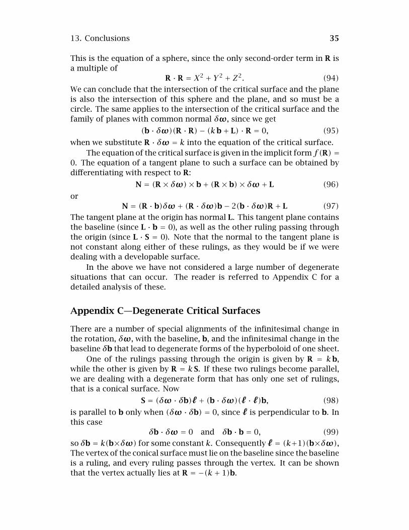
13. Conclusions 35
This is the equation of a sphere, since the only second-order term in R isa multiple of
R · R = X2 + Y 2 + Z2. (94)We can conclude that the intersection of the critical surface and the planeis also the intersection of this sphere and the plane, and so must be acircle. The same applies to the intersection of the critical surface and thefamily of planes with common normal δωω, since we get
(b · δωω)(R · R)− (kb+ L) · R = 0, (95)when we substitute R · δωω = k into the equation of the critical surface.
The equation of the critical surface is given in the implicit form f(R) =0. The equation of a tangent plane to such a surface can be obtained bydifferentiating with respect to R:
N = (R × δωω)× b+ (R × b)× δωω+ L (96)or
N = (R · b)δωω+ (R · δωω)b− 2(b · δωω)R + L (97)The tangent plane at the origin has normal L. This tangent plane containsthe baseline (since L · b = 0), as well as the other ruling passing throughthe origin (since L · S = 0). Note that the normal to the tangent plane isnot constant along either of these rulings, as they would be if we weredealing with a developable surface.
In the above we have not considered a large number of degeneratesituations that can occur. The reader is referred to Appendix C for adetailed analysis of these.
Appendix C—Degenerate Critical Surfaces
There are a number of special alignments of the infinitesimal change inthe rotation, δωω, with the baseline, b, and the infinitesimal change in thebaseline δb that lead to degenerate forms of the hyperboloid of one sheet.
One of the rulings passing through the origin is given by R = kb,while the other is given by R = kS. If these two rulings become parallel,we are dealing with a degenerate form that has only one set of rulings,that is a conical surface. Now
S = (δωω · δb) + (b · δωω)( · )b, (98)is parallel to b only when (δωω · δb) = 0, since is perpendicular to b. Inthis case
δb · δωω = 0 and δb · b = 0, (99)so δb = k(b×δωω) for some constant k. Consequently = (k+1)(b×δωω),The vertex of the conical surface must lie on the baseline since the baselineis a ruling, and every ruling passes through the vertex. It can be shownthat the vertex actually lies at R = −(k+ 1)b.
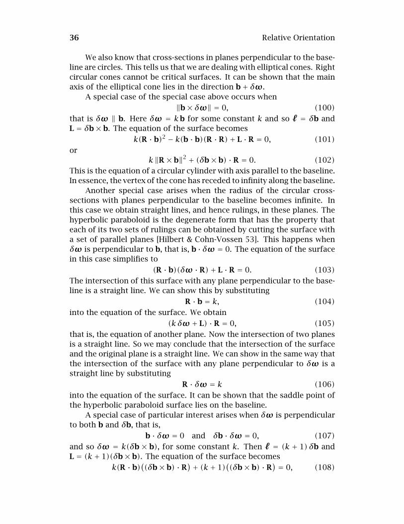
36 Relative Orientation
We also know that cross-sections in planes perpendicular to the base-line are circles. This tells us that we are dealing with elliptical cones. Rightcircular cones cannot be critical surfaces. It can be shown that the mainaxis of the elliptical cone lies in the direction b+ δωω.
A special case of the special case above occurs when
‖b× δωω‖ = 0, (100)that is δωω ‖ b. Here δωω = kb for some constant k and so = δb andL = δb× b. The equation of the surface becomes
k(R · b)2 − k(b · b)(R · R)+ L · R = 0, (101)or
k‖R × b‖2 + (δb× b) · R = 0. (102)This is the equation of a circular cylinder with axis parallel to the baseline.In essence, the vertex of the cone has receded to infinity along the baseline.
Another special case arises when the radius of the circular cross-sections with planes perpendicular to the baseline becomes infinite. Inthis case we obtain straight lines, and hence rulings, in these planes. Thehyperbolic paraboloid is the degenerate form that has the property thateach of its two sets of rulings can be obtained by cutting the surface witha set of parallel planes [Hilbert & Cohn-Vossen 53]. This happens whenδωω is perpendicular to b, that is, b ·δωω = 0. The equation of the surfacein this case simplifies to
(R · b)(δωω · R)+ L · R = 0. (103)The intersection of this surface with any plane perpendicular to the base-line is a straight line. We can show this by substituting
R · b = k, (104)into the equation of the surface. We obtain
(kδωω+ L) · R = 0, (105)that is, the equation of another plane. Now the intersection of two planesis a straight line. So we may conclude that the intersection of the surfaceand the original plane is a straight line. We can show in the same way thatthe intersection of the surface with any plane perpendicular to δωω is astraight line by substituting
R · δωω = k (106)into the equation of the surface. It can be shown that the saddle point ofthe hyperbolic paraboloid surface lies on the baseline.
A special case of particular interest arises when δωω is perpendicularto both b and δb, that is,
b · δωω = 0 and δb · δωω = 0, (107)and so δωω = k(δb × b), for some constant k. Then = (k + 1)δb andL = (k+ 1)(δb× b). The equation of the surface becomes
k(R · b)((δb× b) · R
)+ (k+ 1)((δb× b) · R
) = 0, (108)

13. Conclusions 37
or just (k(R · b)+ (k+ 1)
)((δb× b) · R
) = 0. (109)so either
(δb× b) · R = 0 or k(R · b)+ (k+ 1) = 0. (110)The first of these is the equation of a plane containing the baseline band the vector δb. The second is the equation of a plane perpendicularto the baseline. So the solution degenerates in this case into a surfaceconsisting of two intersecting planes. One of these planes appears onlyas a line in each of the two images, since it passes through both projectioncenters, and so does not really contribute to the image. It is fortunate thatplanes can only be degenerate surfaces if they are perpendicular to thebaseline, since surfaces that are almost planar occur frequently in aerialphotography22.
To summarize then, we have the following degenerate cases:
• elliptical cones when δωω ⊥ δb,
• circular cylinders when δωω ‖ b,
• hyperbolic paraboloids when δωω ⊥ b,
• intersecting planes when δωω ⊥ δb and δωω ⊥ b.
For further details, and a proof that not all hyperboloids of one sheetpassing through the origin lead to critical surfaces, see [Horn 87b].
22The baseline was nearly perpendicular to the surface in the sequence of pho-tographs obtained by the Ranger spacecraft as it crashed into the lunar surface.This made photogrammetric analysis difficult.