Relative Hazard Calculation Methodology

PNNL-12008Rev. 0

Relative Hazard CalculationMethodology

R. D. StennerM. K. WhiteD. L. StrengeW. B. Andrews

February 1999

Prepared for theOffice of Science and Risk PolicyU.S. Department of EnergyOffice of Environmental ManagementandCenter for Risk ExcellenceU.S. Department of EnergyChicago Operations Office

Prepared for the U.S. Department of Energyunder Contract DE-AC06-76RLO 1830

DISCLAIMER

This report was prepared as an account of work sponsored by an agency of theUnited States Government. Neither the United States Government nor anyagency thereof, nor Battelle Memorial Institute, nor any of their employees,makes any warranty, express or implied, or assumes any legal liability orresponsibility for the accuracy, completeness, or usefulness of anyinformation, apparatus, product, or process disclosed, or represents thatits use would not infringe privately owned rights. Reference herein to anyspecific commercial product, process, or service by trade name, trademark,manufacturer, or otherwise does not necessarily constitute or imply itsendorsement, recommendation, or favoring by the United States Governmentor any agency thereof, or Battelle Memorial Institute. The views and opinionsof authors expressed herein do not necessarily state or reflect those of theUnited States Government or any agency thereof.

PACIFIC NORTHWEST NATIONAL LABORATORYoperated byBATTELLE

for theUNITED STATES DEPARTMENT OF ENERGY

under Contract DE-AC06-76RLO 1830

Printed in the United States of America

Available to DOE and DOE contractors from theOffice of Scientific and Technical Information, P.O. Box 62, Oak Ridge, TN 37831;

prices available from (615) 576-8401.

Available to the public from the National Technical Information Service,U.S. Department of Commerce, 5285 Port Royal Rd., Springfield, VA 22161

This document was printed on recycled paper.

(9/97)

PNNL-12008Rev. 0

Relative Hazard Calculation Methodology

R. D. StennerM. K. WhiteD. L. StrengeW. B. Andrews

February 1999

Prepared for theOffice of Science and Risk PolicyU.S. Department of EnergyOffice of Environmental ManagementandCenter for Risk ExcellenceU.S. Department of EnergyChicago Operations Office

Pacific Northwest National LaboratoryRichland, Washington 99352

iii

Acknowledgments

The authors wish to acknowledge and thank Mark Gilbertson and the Department of Energy-Office ofScience and Risk Policy (DOE/EM-52) for the insight to fund and promote the development of thisdocument.

Also, a special acknowledgment and thanks go to Al Young and Mark Bollinger of the Department ofEnergy-Center for Risk Excellence (CRE), and the CRE Board, for identifying the need, through thedevelopment of the site risk profiles, for the methodology addressed by the document. They alsoprovided funding and support for the application of this methodology to site-specific risk profiles, whichhelped to iteratively develop the methodology using real site cases.

The authors also wish to acknowledge and thank Bruce Napier (PNNL) for providing peer review andexcellent technical suggestions for improving the document.

v

Contents

Acknowledgments ........................................................................................................................ iii

1.0 Introduction .......................................................................................................................... 1.1

2.0 Relative Hazard Calculation.................................................................................................. 2.1

2.1 Quantity Data ............................................................................................................... 2.2

2.2 Release Fraction .......................................................................................................... 2.2

2.3 Hazard Measure Factors ............................................................................................... 2.3

2.3.1 Radionuclides..................................................................................................... 2.3

2.3.2 Hazardous Chemicals ......................................................................................... 2.9

2.4 Hazard Control Factors................................................................................................. 2.10

2.4.1 Hazard Versus Risk............................................................................................ 2.12

2.4.2 Factors Affecting the HC.................................................................................... 2.13

2.4.3 Approach for Estimating HCs............................................................................. 2.14

2.5 Approach to Calculating Relative Hazard Ratios Using the RelativeHazard Equation ........................................................................................................... 2.23

3.0 Application Examples........................................................................................................... 3.1

3.1 Example Site #1............................................................................................................ 3.1

3.1.1 Surface Contamination Calculation Notes........................................................... 3.1

3.1.2 Sub-Surface Contamination Calculation Notes ................................................... 3.4

3.1.3 Waste Disposal Operations Calculation Notes .................................................... 3.6

3.1.4 References ......................................................................................................... 3.8

vi

3.2 Example Site #2............................................................................................................ 3.8

3.2.1 Nuclear Materials Calculation Notes .................................................................. 3.8

3.2.2 Transuranic Waste Calculation Notes ................................................................. 3.10

3.2.3 Low-Level Waste and Mixed Low-Level Waste Calculation Notes..................... 3.12

4.0 Summary .......................................................................................................................... 4.1

5.0 References .......................................................................................................................... 5.1

vii

Figures

3.1 Surface Contamination Calculated for Example Site #1......................................................... 3.4

3.2 Sub-Surface Contamination Calculated for Example Site #1 ................................................. 3.5

3.3 Waste Disposal Calculations for Example Site #1 ................................................................. 3.7

3.4 Nuclear Material Relative Hazards Calculated for Example Site #2....................................... 3.10

3.5 Transuranic Waste Relative Hazards Calculated for Example Site #2 .................................... 3.12

3.6 LLW and LLMW Relative Hazards Calculated for Example Site #2 ..................................... 3.15

viii

Tables

2.1 Air Exposure Pathway Groups for Radionuclides ................................................................. 2.5

2.2 Surface Water Exposure Pathway Groups for Radionuclides ................................................. 2.6

2.3 Partition Coefficients (Kds) and Derived Groundwater Transfer Coefficients Usedin the Groundwater Exposure Pathway Radionuclide Categories ........................................... 2.7

2.4 Groundwater-to-Surface Water Exposure Pathway Groups for Radionuclides ....................... 2.8

2.5 Fire/Explosion Exposure Pathway Groups for Radionuclides ................................................ 2.8

2.6 Direct Contact Exposure Pathway Groups for Radionuclides................................................. 2.9

2.7 Hazard Measures for Chemicals Based on Reportable Quantity............................................. 2.10

2.8 Hazard Measures Determination for Representative Constituents .......................................... 2.11

2.9 Hazard Reduction Measures with Generic Hazard Control Factors........................................ 2.16

2.10 Contaminant Categories........................................................................................................ 2.17

2.11 Hanford Hazard Control Factor Parameters........................................................................... 2.19

2.12 INEEL Hazard Control Factor Parameters............................................................................. 2.20

2.13 Rocky Flats Hazard Control Factor Parameters ..................................................................... 2.21

2.14 Savannah River Hazard Control Factor Parameters ............................................................... 2.22

3.1 Sub-Surface Inventory .......................................................................................................... 3.2

3.2 Surface Inventory ............................................................................................................. 3.2

1.1

1.0 Introduction

In February 1997, the Center for Risk Excellence (CRE) was created and charged as a technical,field-based partner to the Office of Science and Risk Policy (EM-52). One of the initial charges to theCRE was to assist the sites in the development of “site risk profiles.” These profiles were to be relativelyshort summaries (periodically updated) with a broad perspective on the major risk-related challenges thatface the respective site. The risk profile serves as a high-level communication tool for interested internaland external parties to enhance the understanding of these risk-related challenges. The risk profile foreach site has been designed to qualitatively present the following information: 1) a brief overview of thesite, 2) a brief discussion on the historical mission of the site, 3) a quote from the site manager indicatingthe site’s commitment to risk management, 4) a listing of the site’s top risk-related challenges, 5) a briefdiscussion and detailed table presenting the site’s current risk picture, 6) a brief discussion and detailedtable presenting the site's future risk reduction picture, and 7) illustrations of the projected management ofthe relative hazards at the site. During fiscal year 1998, risk profiles for the Richland Operations Office(DOE 1998a), Nevada Operations Office (DOE 1998b), Rocky Flats Field Office (DOE 1998c),Savannah River Operations Office (DOE 1998d), and Albuquerque Operations Office (DOE 1998e) weredeveloped, which used the methodology discussed in this report.

The illustrations were included to provide the reader of the risk profiles with a high-level mentalpicture to associate with all the qualitative information presented in the risk profile. This report presentsthe methodology developed to produce the graphics showing the relative hazard reductions that occur as aresult of a site's projected risk management actions.

The term “controlling constituent” is used often in this document. Controlling constituents aredefined as those radionuclides and/or hazardous chemicals in a particular waste type that tend to controlits environmental impact or hazardousness of the consequences associated with the waste material. In theanalysis methods discussed in this document, it is advantageous to limit the number of controllingconstituents to as few as possible and still adequately represent the hazardousness of the waste material.In most risk assessments, there are usually just one or two constituents that tend to drive the risk. It isthese constituents that we are calling “controlling constituents.”

2.1

2.0 Relative Hazard Calculation

The methodology consists of 1) using site-specific information (e.g., information from site dispositionmaps, site-specific Project Baseline Summaries (PBSs), and other site documents that address elements ofthe overall risk story for a site) and 2) applying factors from applicable site-specific risk assessmentresults or look-up tables to generate relative hazard (RH) ratio values by waste type.

Relative hazard calculations are made using the following relationship of key risk-related parametersthat can be extracted from the information provided for the risk profiles:

0tcccctcct0cctcct0ccctcct0cct HC/HCHM/HMRF/RFQ/Q(RH)HazardRelativen

1cc

∗∗∗= ∑=

(2.1)

where Qcct = quantity of the controlling constituents (radionuclides, in curies and hazardouschemicals, in kilograms) at time t (i.e., time when specified risk management actionis completed)

Qcct0 = quantity of the controlling constituents (radionuclides, in curies and hazardouschemicals, in kilograms) at time t0 (i.e., the original baseline or starting time)

RFcct = fraction of controlling constituent quantity that is releasable to the controllingpathway at time t

RFcct0 = fraction of the controlling constituent quantity that is releasable to the controllingpathway at time t0

HMcct = hazard measure factor for controlling constituent and controlling pathway at time t(hazard measure factors from look-up tables)

HMcct0 = hazard measure factor for controlling constituent and controlling pathway at time t0(hazard measure factors from look-up tables)

HCcct = hazard control factor for risk management control action specific at time t (hazardcontrol factors may be estimated from site risk data or approximated using suppliedlook-up tables)

HCcct0 = hazard control factor for risk management control action specific at time t0 (hazardcontrol factors may be estimated from site risk data or approximated using suppliedlook-up tables)

n = number of controlling constituents.

2.2

Note: If only one controlling constituent is identified (highly encouraged), the equation will not need tobe summed over the number of controlling constituents.

The RH equation calculates a relative ratio, which represents a hazard reduction resulting from aspecified risk management action compared to a baseline. It does not calculate an absolute hazard value.At this time, the level of data available in the disposition maps and PBSs are not detailed enough tosupport the calculation of absolute hazard values. The current state is the baseline to which each riskmanagement action is compared. The baseline factor is designated as time-zero (t0) in subscripts and riskmanagement factors at subsequent times (t). To compare each risk management action step with theprevious risk management action time step, the baseline factors (i.e., factorcct0) can simply be replacedwith the corresponding previous time factor (i.e., factorcct-1). Each factor of the RH equation is discussedseparately below.

2.1 Quantity (Q) Data

The best available site-specific quantity data should be used when calculating the RH ratios. In orderfor the RH ratios to be comparable across the different waste types, the quantity data should be specific toeach controlling constituent and should be provided in units of curies for radionuclides or grams forhazardous chemicals. If exact amounts of each controlling constituent are not available, rough estimatesof the fraction of each controlling constituent contained in the total waste quantity can be made. Thesefractions can then be used to adjust the total waste quantity to estimate the quantity of each respectivecontrolling constituent. If controlling constituent quantity data in curies (radionuclides) or grams(hazardous chemicals) are just not available and it is not possible to estimate the fractions of eachcontrolling constituent in the total waste quantity, the total waste quantity of each waste type can be usedas a rough surrogate, provided that units of this quantity remain the same through out the analysis of therespective waste type. However, without controlling constituent quantities, the RH result would generallybe non-comparable across waste types. The RH ratios may not be accurate for risk management actionsthat involve treatment of the controlling constituent(s).

2.2 Release Fraction (RF)

In some cases, the total quantity of a controlling constituent is not all releasable to the controllingexposure pathway of concern (i.e., dominant exposure pathway). In these cases, a release fraction (i.e.,the fraction of the total quantity of the controlling constituent that is releasable to the controlling pathway)should be provided for use in the RH equation to adjust the quantity. Use of a release fraction allows onlythe fraction of the controlling constituent quantity that can actually be released to the exposure pathway tobe considered. If all of the controlling constituent quantities are available for release to the controllingexposure pathway, which is true for many waste type situations, the RF factor can be assigned a valueof 1.

2.3

2.3 Hazard Measure (HM) Factors

The HM considers the inherent toxicity or carcinogenic potential of the controlling contaminantsidentified, as well as its potential to expose members of the public through various exposure pathways.Because constituents then are determined a priori, the HM factors, along with Q data, is probably one ofthe least subjective of the RH equation factors. The HM factor look-up tables are provided.

The HM factors were derived differently for radionuclides and chemicals. Chemical HMs were baseddirectly on the reportable quantities (RQs) of 40 CFR Part 302, “Designation, Reportable Quantities, andNotification.” Radionuclide HMs were determined for five exposure pathways using ICRP-30 dosecalculation methods and near-field exposure modeling assumptions. Derivation of these radionuclideHMs was based on a method developed for the Modified Hazard Ranking System (Hawley and Napier1985; Hawley et al. 1986; Stenner et al. 1986). Because radionuclide and chemical HMs are determineddifferently, details of the two methods and differences between them are discussed below.

2.3.1 Radionuclides

The HM for radionuclides are similar to an exposure pathway-specific dose factor although themodeling is not detailed enough to provide an absolute dose estimate. The Modified Hazard RankingSystem (MHRS), the original use of radionuclide HMs, was developed to work within the framework ofthe EPA’s Hazard Ranking System (HRS) (EPA 1982). However, the MHRS also provides a moreappropriate treatment of radionuclides in ranking mixed waste sites for the National Priority List underthe Comprehensive Environmental Response, Compensation, and Liability Act (CERCLA). Like theMHRS and HRS, radionuclides are evaluated under five potential exposure pathways: air, surface water,groundwater, fire/explosion, and direct contact.

Designed for generic application anywhere the HRS could be used, the MHRS included a limitedsuite of radionuclides and used the ICRP Publication 2 (ICRP 1959) “critical organ” concept in assigninga potential “hazard ranking” to radionuclides. Like the MHRS-based factors, however, the RH-based HMfactors are based upon near-field scenarios. In a near-field scenario, interest is focused on the doses anindividual could receive at a particular location as a result of initial contamination or external sources(i.e., buried solid waste, contaminated soil, contaminated water, or contamination in air).(a) Near-fieldassumptions were used, since the basic difference between near-field and far-field scenarios is dilution.In an RH analysis, the affect of dilution distance can be accounted for in the hazard control (HC)parameter associated with relocation of material further from a receptor.

(a) This differs from a far-field scenario, defined as determining impacts of a particular release of

radioactive or hazardous material into a wide environment, such as the dose from releases from astack to individuals or populations downwind.

2.4

While the MHRS approach was retained, several enhancements were made to the HM factorspresented for use in the RH calculations:

Additional radionuclides are included. Like the MHRS-based factors, the RH-based factors aregenerally limited to radionuclides with a half-life of 1 year or greater, unless they were specificallynoted as being potentially important in one of the waste materials being considered.

• The dose calculation methodology was updated to ICRP Publication 30 (ICRP 1979), using theGENII computer codes (Napier et al. 1988a; 1988b; 1988c) to perform updated calculations for thefive exposure pathways. Radionuclide HMs are now based upon effective dose equivalent (EDE)rather than critical organ dose.

• The methodology used to produce the RH-based HM values utilized default inputs of the GENIIcode, and, for the groundwater exposure pathway, used groundwater transfer partition coefficients(Kd) from Serne and Wood (1990).

Descriptions of the exposure assumptions and radionuclide categories for each of the five exposurepathways are provided in the sections below, along with the respective HM factor look-up tables. In eachexposure pathway table, radionuclides are categorized by the approximate dose received per unitconcentration. Each category differs from the others by approximately an order of magnitude in the“relative dose impact.” All exposure-pathway-specific HM-factor tables have been normalized, so thatthe highest category is V and the lowest is 0, corresponding to the exponent of the value of the HM factorassigned to each category (i.e., category V has an HM value of 100,000, while category 0 has an HMvalue of 1).

2.3.1.1 Air Exposure Pathway

This is a chronic exposure pathway that primarily poses long-term, large-scale risks to the public.Assumptions are that the exposed individual:

• lives continuously in contaminated air (chronic inhalation)

• is continuously exposed to external radiation from radionuclides deposited on the ground surface

• is continuously immersed in the airborne radioactive plume.

The values of the HM factor for the air exposure pathway are given in Table 2.1 for selectedradionuclides.

2.5

Table 2.1. Air Exposure Pathway Groups for Radionuclides

CategoryHazard

Measure (HM) Radionuclide Grouping

V 105 22Na, 54Mn, 60Co, 94Nb, 125Sb, 134Cs, 137Cs, 152Eu, 154Eu

IV 104 155Eu, 232Th, 233U, 234U, 235U, 238U, 237Np, 239Np, 238Pu, 239Pu,240Pu, 241Am, 243Cm, 244Cm, 245Cm

III 103 10Be, 36Cl, 109Cd, 129I, 241Pu, 226Ra, 242Cm, 252Cf

II 100 55Fe, 59Ni, 90Sr, 93Mo, 99Tc, 147Pm

I 10 14C, 135Cs, 151Sm

0 1 3H, 63Ni

2.3.1.2 Surface-Water Exposure Pathway

This is a chronic exposure pathway that primarily poses long-term risks to public users of localsurface water sources. Assumptions are that the exposed individual:

• eats food irrigated with contaminated surface water, at an irrigation rate of 150 L/m2/mo for 6 mo/y

• eats fish from the contaminated water

• is exposed to external radiation from contaminated sediments along the bank

• gets drinking water from the contaminated surface water.

Resuspension and external radiation from radionuclides deposited on the soil from irrigation are notconsidered. The values of the HM factor for the surface-water exposure pathway are given in Table 2.2for selected radionuclides.

2.3.1.3 Groundwater-to-Surface-Water Exposure Pathway

This is a chronic exposure pathway that primarily poses long-term risks to public users of the localsurface water sources. Groundwater is assumed to connect with surface water through infiltration, andexposure is via the surface water exposure pathway. No direct groundwater exposure via groundwaterwells is assumed. Assumptions are that the exposed individual:

• eats food irrigated with surface water contaminated via connection with groundwater, at an irrigationrate of 150 L/m2/mo for 6 mo/y

• eats fish from the contaminated water

2.6

Table 2.2. Surface Water Exposure Pathway Groups for Radionuclides

CategoryHazard


V 105 134Cs, 137Cs, 237Np

IV 104 129I, 135Cs, 226Ra, 232Th, 241Am, 243Cm, 244Cm, 245Cm, 252Cf

III 103 14C, 22Na, 36Cl, 60Co, 109Cd, 152Eu, 154Eu, 233U, 234U, 235U,238U, 239Np, 238Pu, 239Pu, 240Pu, 242Cm

II 100 10Be, 54Mn, 55Fe, 63Ni, 90Sr, 94Nb, 99Tc, 125Sb, 147Pm, 151Sm,155Eu, 241Pu

I 10 59Ni, 93Mo

0 1 3H

• is exposed to external radiation from contaminated sediments along the bank

• gets drinking water from the contaminated surface water.

Resuspension and external radiation from radionuclides deposited on the soil from irrigation are notconsidered.

The groundwater-to-surface-water exposure pathway radionuclide categories were adjusted for thetendency of radionuclides to adsorb to soil particles (partition coefficient, Kd) during groundwatertransport. Partition coefficients were obtained (Serne and Wood 1990) and converted to groundwatertransfer coefficients from 1 to 100 (Hawley and Napier 1985; Hawley et al. 1986) to be consistent withthe multiplicative RH strategy. The Kd values used for each radionuclide and the derived groundwatertransfer coefficients are shown in Table 2.3. The HM factor for groundwater does not consider the time ittakes the radionuclide to move through the vadose zone to the saturated zone and to a point where it couldfit the near-field scenario. The values of the HM factor for the groundwater-to-surface-water exposurepathway are given in Table 2.4 for selected radionuclides.

2.3.1.4 Fire/Explosion Pathway

The fire/explosion pathway is also intended to represent non-energetic acute releases resulting fromfacility accident sequences. This acute exposure pathway primarily poses near-term, large-scale publichealth risks. Assumptions are as follows:

• Exposure lasts only a short time, approximately 0.5 hour, with the exposed individual at the centerline of the released plume.

• The only relevant pathway is inhalation; to account for the high concentration of material in theplume, it was modeled as resuspension with a mass loading of 1 g/m3.

2.7

Table 2.3. Partition Coefficients (Kds) and Derived Groundwater Transfer Coefficients Usedin the Groundwater Exposure Pathway Radionuclide Categories

Constituent/Radionuclide Kd

Groundwater TransferCoefficient

3H 0(a) 100

Be 30(b) 314C 0(a) 100

Na 3(a) 33

Cl 0(a) 100

Mn 20(a) 5

Fe 20(a) 5

Co 10(a) 10

Ni 15(a) 7

Sr 10(a) 10

Sb 0(b) 100

Nb 100(b) 1

Mo 0(a) 100

Tc 0(a) 100

Cd 15(a) 7

I 0(a) 100

Cs 50(a) 2

Lanthanides Eu, Pm, Sm 50(a) 2

Ra 20(a) 5

Th 50(a) 2

U 0(a) 100

Np 3(a) 33

Pu 100(a) 1

Am, Cm 100(a) 1

Ac, Cf 100(b) 1

(a) Serne and Wood (1990).

(b) Serne (1994).

2.8

Table 2.4. Groundwater-to-Surface Water Exposure Pathway Groups for Radionuclides

CategoryHazard


V 105 237Np

IV 104 129I

III 103 14C, 36Cl, 134Cs, 137Cs, 232Th, 233U, 234U, 235U, 238U, 239Np,241Am

II 100 22Na, 60Co, 99Tc, 125Sb, 135Cs, 226Ra, 243Cm, 244Cm, 245Cm,252Cf

I 10 54Mn, 55Fe, 90Sr, 109Cd, 152Eu, 154Eu, 238Pu, 239Pu, 240Pu,242Cm

0 1 3H, 10Be, 59Ni, 63Ni, 94Nb, 93Mo, 147Pm, 151Sm, 155Eu, 241Pu

The values of the HM for the fire/explosion exposure pathway are given in Table 2.5 for keyradionuclides.

Table 2.5. Fire/Explosion Exposure Pathway Groups for Radionuclides

CategoryHazard


V 105 232Th, 233U, 234U, 235U, 238U, 237Np, 238Pu, 239Pu, 240Pu,241Am, 243Cm, 244Cm, 245Cm, 252Cf

IV 104 22Na, 54Mn, 60Co, 94Nb, 125Sb, 134Cs, 137Cs, 152Eu, 154Eu,226Ra, 241Pu, 242Cm

III 103 10Be, 90Sr, 109Cd, 129I, 155Eu, 239Np

II 100 36Cl, 93Mo, 99Tc, 135Cs, 147Pm, 151Sm

I 10 14C, 55Fe, 59Ni, 63Ni

0 1 3H

2.3.1.5 Direct Contact Exposure Pathway

This is an acute exposure pathway that primarily poses near-term risks to individual workers ormembers of the public. Assumptions are as follows:

• The exposed individual is in direct contact with the material for a short period of time, approximately1 hour, while digging or otherwise creating loose material airborne.

• Exposure pathways are inhalation, external exposure, and resuspension of loose material with massloading of 0.0001 g/m3.

2.9

The values of the HM factor for the direct contact exposure pathway are given in Table 2.6 for selectedradionuclides.

Table 2.6. Direct Contact Exposure Pathway Groups for Radionuclides

CategoryHazard


V 105 22Na, 54Mn, 60Co, 94Nb, 125Sb, 134Cs, 137Cs, 152Eu, 154Eu

IV 104 155Eu, 232Th, 233U, 234U, 235U, 238U, 237Np, 239Np, 238Pu, 239Pu,240Pu, 241Am, 243Cm, 244Cm, 245Cm, 252Cf

III 103 109Cd, 129I, 226Ra, 241Pu, 242Cm

II 100 10Be, 36Cl, 55Fe, 59Ni, 90Sr, 93Mo

I 10 14C, 63Ni, 99Tc, 135Cs, 147Pm, 151Sm

0 1 3H

2.3.2 Hazardous Chemicals

The HM factor values for hazardous chemicals are based on the RQs of 40 CFR Part 302.4,“Designation of Hazardous Substances.” According to the EPA, “RQs represent a determination only ofpossible or potential harm, not that releases of a particular amount of a hazardous substances willnecessarily be harmful to the public health or welfare or to the environment.” The RQs provide a simple,readily available method of comparing the potential hazard from a specific set of chemicals.

The RQ-derived HMs for hazardous chemicals are fundamentally different from the HMs forradionuclides in that the RQs are not exposure-pathway specific. Their primary criteria for evaluation areaquatic toxicity, mammalian toxicity (oral, dermal, and inhalation), ignitability, reactivity, chronictoxicity, and potential carcinogenicity.

The HMs for chemicals were derived from the RQs as shown in Table 2.7. An adjustment was madeto maintain a multiplicative scheme for the RH strategy. Relationships between the various RQs andHMs are maintained by this adjustment.

Table 2.7. Hazard Measures for Chemicals Based on Reportable Quantity

Category RQ HMA 1 1000B 10 100C 100 10D 1000 1E 5000 0.5

2.10

Not all chemicals identified for the various DOE facilities and areas will have RQs listed in40 CFR 302. Some HM values were derived by comparison to similar chemicals. When no values of RQare available for a specific key chemical, surrogate values of HM can be developed using RQ values froma chemical with similar transport (Kd, Koc, Kow, solubility limit, etc.) and toxicity (e.g., slope factors andreference doses). Transport and toxicity parameter values can be reviewed using the Multimedia-Modeling Environmental Database Editor (Warren and Strenge 1994), which accesses the MultimediaEnvironmental Pollution Assessment System (MEPAS) database (Strenge and Peterson 1989). Table 2.8provides a list of constituents of possible importance to DOE sites and indicates the use of surrogatechemicals in several instances. The table lists current RQ values from 40 CFR 302 for several chemicals,with HM values determined using the convention of Table 2.7. For those chemicals not included in40 CFR 302, the estimated HM is given with an indication of the basis. For example, values for thealcohols ethanol and isopropanol are set to the value for methanol because of chemical similarity. TheHM values for benzo(b)fluoranthene and benzo(k)fluoranthene were estimated from the HM ofbenzo(a)pyrene and the toxicity equivalence among the three compounds. From the MEPAS database,the oral slope factors for the three chemicals are:

benzo(a)pyrene 7.3 kg-d/mgbenzo(b)fluoranthene 0.73 kg-d/mgbenzo(k)fluoranthene 0.073 kg-d/mg

The HM for benzo(a)pyrene is multiplied by the chemical oral slope factor and divided by thebenzo(a)pyrene slope factor to estimate the HM for the chemical. The inorganic chemicals in the list areassumed to be in ionic form. Some of these are expected to be in relatively non-toxic forms in theenvironment (e.g., sodium, potassium, magnesium, and nitrate) and have HM values set to the minimumvalue (0.5) from Table 2.7.

2.4 Hazard Control Factors

The hazard control (HC) factors represent the worth, in terms of reduction in hazard, of specific riskmanagement actions. These actions include

• risk management activities such as vitrification or grouting of waste materials

• separation, reduction and/or removal of specific constituents from a waste stream

• relocation of waste material away from receptors or vulnerable pathways

• repackaging and/or stabilization of waste material.

In calculating the RH of a waste type at a site, it is recommended that these HC factors be estimatedfrom existing risk assessment data, where possible. In many cases, there will be specific risk assessmentsfor which generalizations can be made to roughly estimate the worth of a specific risk managementaction. Often, there are risk estimates for specified accident conditions in a Safety Analysis Report (SAR)

2.11

Table 2.8. Hazard Measures Determination for Representative Constituents

CAS Name Final RQ HM HM Basis56235 Carbon Tetrachloride 10 100 RQ

67561 Methanol 5000 0.5 RQ

64175 Ethanol -- 0.5 Methanol HM

67630 Isopropanol -- 0.5 Methanol HM

75058 Acetonitrile 5000 0.5 RQ

91203 Naphthalene 100 10 RQ

91576 2-Methylnaphthalene -- 10 Naphthalene HM

107211 Ethylene glycol 5000 0.5 RQ

110543 Hexanes 5000 0.5 RQ

117817 Bis(2-ethylhexyl)phthalate 100 10 RQ126738 Tributylphosphate -- 10 Tetrachloroethylene HM

127184 Tetrachloroethylene 100 10 RQ

79016 Trichloroethylene 100 10 RQ

50328 Benzo(a)pyrene 1 1000 RQ

205992 Benzo(b)fluoranthene -- 100 Benzo(a)pyrene HM and toxicityequivalence

207089 Benzo(k)fluoranthene -- 10 Benzo(a)pyrene HM and toxicityequivalence

1809194 Dibutyl Phosphate -- 10 Tetrachloroethylene HM

6834920 Silica -- 0.5 Minimum HM value

7429905 Aluminum ion 5000 0.5 RQ for aluminum sulfate7439987 Molybdenum ion -- 1 HM value for chromium III and VI

7440393 Barium 1000 1 RQ

7440473 Chromium VI ion 1000 1 RQ for chromic acetate and sulfate

7440611 Uranium ion 100 10 RQ for uranyl acetate and nitrate

7440622 Vanadium ion 1000 1 RQ for vanadium compounds

7440677 Zirconium ion 5000 0.5 RQ for zirconium compounds

7440702 Calcium ion -- 0.5 Minimum HM value

7447407 Potassium ion -- 0.5 Minimum HM value

7447418 Lithium ion 10 100 RQ for lithium chromate

7601549 Phosphate ion 5000 0.5 RQ for phosphoric acid

7647145 Sodium ion -- 0.5 Minimum HM value

7782414 Fluoride ion 1000 1 RQ for fluorides of sodium and zinc

7786303 Magnesium ion -- 0.5 Minimum HM value

12808798 Sulfate ion -- 0.5 Minimum HM value

14797558 Nitrate ion -- 0.5 Minimum HM value

15438310 Iron ion 1000 1 RQ for ferric chloride and sulfate

16065831 Chromium III ion 1000 1 RQ for chromus chloride

14797650 Nitrite ion 1000 1 RQ for sodium nitrite

7440360 Antimony ion 1000 1 RQ for common antimony salts

2.12

or safety basis document that can be examined to get a rough estimate of the worth of a specific action. Incases where no such risk assessment data are available, HC look-up tables are provided to use inestimating the HC factor.

The HC factor is used to assess changes in the relative hazard of a contaminant or waste based onchanges in its physical condition or location due to waste management or environmental restorationactions. The HC factor for a specific hazard reduction measure (e.g., capping) represents the reduction inhazard associated with that measure (i.e., the post-action hazard divided by the pre-action hazard). Inconjunction with the other factors representing contaminant inventory, the nature of the contaminant, andpotential contaminant exposure mechanism, the HC factor allows evaluation of the potential reduction inhazard associated with a variety of potential waste management or environmental restoration actions.

2.4.1 Hazard Versus Risk

The term “hazard” as used here relates to potential health effects associated with a contaminant orwaste material, assuming that it is already released to the environment. In contrast, the estimates of risktypically used to assess the need for or effectiveness of environmental restoration or waste managementactivities assume potential health effects and likelihood of contaminant release and subsequent exposure.In simple terms, hazard and risk are related as follows:

Risk =Probability ofRelease orExposure

X Hazard

Therefore, the term “hazard” as used here relates only to the intrinsic danger to health that would beposed by the contaminant or waste material in the environment in its current physical form and location.Changes in physical form or location of a contaminant or waste that alter its hazard can also change itsassociated risk. However, it is not necessarily true that that a contaminant or waste with a relatively highhazard poses a high risk in the sense that is usually discussed in “risk assessments.”

This relationship between risk and hazard can be used to facilitate calculating HCs. If the risks arecompared for a contaminant or waste in differing physical conditions or locations but having the sameprobability of release or exposure, the relative hazards are related in the same proportion as the relativerisks.

Therefore, standard risk-estimating techniques that make the probability of release or exposureconstant allow direct estimation of the change in hazard associated with management or restorationactions. The simplest way to “fix” the probability of release or exposure is to assume that thecontaminant or waste has already been released. This is the approach that was used to estimate thechanges in hazard (i.e., HCs) discussed in the following sections.

2.13

2.4.2 Factors Affecting the HC

Five aspects of a contaminant or waste that have significant impacts relative to assessing its hazardare described in the following sections.

2.4.2.1 Toxicity or Radiological Nature

A contaminant’s toxic or radiological characteristics determine the severity of its health effects whenexposure occurs. Differences among contaminants in this regard are accounted for in the health effectsdata used in risk assessment methodologies. While typical waste management or environmentalrestoration activities may affect the amount of contaminant present, they generally do not affect its toxicor radiological nature. Therefore, this aspect of potential hazard is not addressed in assessing HCs forsuch actions. However, since this factor affects hazard but not HCs, this aspect of hazard is addressed bythe HM factor in the relative hazard calculation.

2.4.2.2 Chemical Nature

The second key aspect of a contaminant affecting its hazard, or the impact of hazard control measureson it, is its chemical nature. Organic and inorganic contaminants generally behave differently both intheir environmental transport and their response to treatment. In addition, the hazard associated with aradioactive elements changes spontaneously as it decays.

2.4.2.3 Mobility

A third aspect of a contaminant or waste affecting its hazard is its mobility in the environment.Contaminants that move more readily through the environment are more likely to be transported tooff-site receptors than those that are relatively immobile. Thereby, they pose greater health risks to thosereceptors. In addition, slow transport of radioactive elements allows time for these contaminants to decayprior to exposing receptors.

2.4.2.4 Physical Form

The physical form of a contaminant or waste has a significant impact on its hazard. The physicalform of a contaminant or waste affects its availability for transport (i.e., the rate at which it is released).For example, liquid wastes are generally easier to transport than solid wastes and, therefore, are morehazardous. In addition, solid waste that has been treated to immobilize contaminants (e.g., cemented orvitrified) allows contaminants to be released more slowly for transport and, therefore, is less hazardous.

2.4.2.5 Location

A contaminant released to the environment in an isolated location with long transport pathways toreceptors is intrinsically less hazardous than the same contaminant in a location that allows rapid transportto receptors. In addition, the hazard reduction associated with a waste management or environmentalrestoration action will vary depending on the waste’s location.

2.14

2.4.3 Approach for Estimating HCs

Calculating site-specific HCs for a variety of potential waste management or environmentalrestoration actions requires taking all these considerations into account. The approach used here is tocompare the calculated risks for site-specific conditions before and after such actions are taken to infer thecorresponding reduction in hazard, as suggested by the relationship between risk and hazard discussedabove.

Such risk calculations can be performed with any risk calculation methodology that allows parametricvariation of the key parameters discussed above. For the illustrative calculations discussed below, theRemedial Action Assessment System (RAAS) was utilized (PNNL 1996). RAAS was developed byPacific Northwest National Laboratory (PNNL) for DOE as an analytical tool for defining and evaluatingalternative remedial action strategies for DOE waste sites. The RAAS methodology is useful for this sortof analysis because it allows direct variation of the key waste form and waste location parametersdescribed above.

The RAAS includes elements of the MEPAS for calculating risk for the maximum exposed individual(MEI) as a result of transport of contaminants to potential receptors (Droppo et al. 1989). Comparison ofthese MEI risks as key waste forms or location factors are varied allows calculation of the correspondingHC.

2.4.3.1 Waste Form Variations

Four different waste forms were analyzed in the following illustrations: liquid waste, soil waste,cemented or grouted waste, and vitrified waste. These classifications represent the most likely forms thatwill be encountered in assessing hazard reduction measures, and many of the key hazard reductionmeasures result in a transition from one of these physical states to another.

The relative hazards associated with these states were calculated by comparing the risk associatedwith equivalent amounts of contaminant already released to the environment. For the solid waste forms(soil waste, cemented or grout wastes, and vitrified waste), in situ wastes of the corresponding wasteforms or states were modeled and the corresponding risk calculated. Since these waste were alreadyreleased, the probability of release or exposure in the risk calculation is the same (i.e., probability ofrelease or exposure is 1.0). Therefore, the relative risks also represent the relative hazards. The liquidwaste state was modeled as a pond containing the same amount of contaminant as the soil site. Again, thecontaminant is modeled as already released, so the corresponding calculated risk can be used to assesschanges in hazard. These calculations, performed for each site of interest, result in the following factorsthat are subsequently used in HC calculations:

risk associated with unit of contaminant in cemented/grouted wasteGF =

risk associated with unit of contaminant in soil waste

risk associated with unit of contaminant in vitrified wasteVF =


2.15

risk associated with unit of contaminant in liquid wasteSF =


2.4.3.2 Hazard Reduction Measures

Hazard controls were estimated for a variety of waste treatment or environmental restoration activitiesinvolving the waste form changes described above. In addition, the following similar factors weredefined or estimated (also using the RAAS methodology) for other actions typically occurring as part ofwaste treatment and environmental restoration:

FMR = Fraction of Medium Removed (in contaminated medium)

FCR = Fraction Contaminant Remaining (after separation/destruction treatment)

risk associated with unit of contaminant in capped siteCF =

risk associated with unit of contaminant in soil waste site

risk associated with unit of contaminant in alternative waste siteRF =

risk associated with unit of contaminant in original soil waste

The first two of these (FMR and FCR) relate to actions that change the inventory or contaminant. Ingeneral, the hazard associated with a contaminant is proportional to its inventory. If waste is removedfrom a contaminated site for treatment, the fraction remaining (1 - FMR) retains its initial hazard level,while the fraction removed (FMR) may have a different hazard level, depending on how it is treated andsubsequently disposed. Note that this formulation assumes that the contaminant removed is proportionalto the medium removed. If this is not the case, then the fraction of the contaminant remaining should beused rather than the fraction of the medium remaining. Similarly, FCR is used to assess the change inhazard associated with in situ or ex situ treatment that separates or destroys the contaminant, therebychanging the contaminant inventory and corresponding hazard. These two factors (i.e., FMR and FCR)are provided to allow the user to make adjustments for inventory reductions within the HC factor;however, these inventory adjustments can also be made by directly adjusting the respective Q values ofthe RH equation. It is left to the user’s discretion to decide where best to account for inventory changesassociated with specific risk/hazard management actions, but care should be taken not to “double count”the inventory reductions. Table 2.9 defines the HCs for a variety of potential waste management orenvironmental restoration actions, in terms of the various hazard reduction factors previously defined.

2.4.3.3 Contaminant Categories

Ideally, the various factors defined above could be calculated for every contaminant of concern andthen used as appropriate to estimate HCs for waste management or environmental restoration actions ofinterest. The RAAS methodology contains the necessary physical, chemical, and health effect data for

2.16

Table 2.9. Hazard Reduction Measures with Generic Hazard Control (HC) Factors

Hazard Reduction Measure HC FactorTreatment to separate or destroycontaminants

1 – FMR(a) (1 – FCR)(b)

Cement/package removed medium 1 – FMR(1 – GF)(c)

Removal, treatment, anddisposal of treated mediumin original environmentalsetting Vitrify/package removed medium 1 – FMR(1 – VF)(d)

Off-site disposal (on treatment) 1 - FMR

Direct disposal in alternative ES on-site 1 – FMR(1 – RF)(e)

Treat to separate or destroy contaminantsand replace in alternative environmentalsetting on-site

1 – FMR[1 – (FCR)(RF)]

Cement/package and replace inalternative environmental setting on-site

1 – FMR[1 – (GF)(RF)]

Removal, treatment, and/orremote disposal of treatedmedium either off-site or inalternative environmentalsetting on-site

Vitrify/package and replace in alternativeenvironmental setting on-site

1 – FMR[1 – (VF)(RF)]

In situ separation/destruction FCR

Grout in place GF

In situ vitrification VF

In situ treatment orcontainment

Capping CF(f)

Solidify liquid waste SF(g)

Separate/destroy contaminants FCR

Cement solid waste GFEx situ waste treatment

Vitrify solid waste VF

(a) FMR = Fraction of contaminated Medium Removed for treatment(b) FCR = Fraction of Contaminant Remaining (final concentration divided by initial

concentration) after treatment to separate or destroyed contaminant(c) GF = Grout Factor = (risk associated with unit of contaminant in grouted waste)/(risk

associated with a unit contaminant in untreated waste)(d) VF = Vitrification Factor = (risk associated with unit of contaminant in vitrified waste)/(risk

associated with a unit of contaminant in untreated waste)(e) RF = Relocation Factor = (risk associated with a unit of contaminant in relocated waste)/(risk

associated with a unit of contaminant in waste in original location)(f) CF = Capping Factor = (risk associated with a unit of contaminant in waste after cap is

applied)/(risk associated with a unit of contaminant in waste in original location prior toapplying cap)

(g) SF = Solidification Factor = (risk associated with unit of contaminant in solidifiedwaste)/(risk associated with a unit of contaminant in liquid waste)

2.17

over 400 organic, inorganic, and radioactive contaminants of potential concern. However, performingsuch comprehensive calculations is time-consuming and probably not warranted in terms of theincremental insight provided. Rather, representative contaminants can be selected and used as surrogatesfor specific contaminants. As discussed previously, the key contaminant-specific differences of concernrelate to the chemical or radiological nature of the contaminant and its mobility.

For the purposes of the illustrative HC estimates developed here, a set of contaminant categories weredeveloped that represent potential variation in these key contaminant characteristics, and a representativecontaminant was selected for each category. These categories and representative contaminants are shownin Table 2.10.

Table 2.10. Contaminant Categories

Low Mobility High Mobility

ContaminantType Organic

Inorganicor LongHalf-Life

Radionuclide

ShortHalf-Life

Radionuclide Organic

Inorganicor Long

Half-LifeRadionuclide

ShortHalf-Life

RadionuclideRepresentativecontaminant(s)

PCBMercury

239Pu137Cs TCE

Arsenic99Tc

3H

2.4.3.4 Illustrative Hazard Control Calculations

The methodology described above was used to develop illustrative HCs for DOE sites, using site-specific information and data.

Site-Specific Data and Information. Illustrative hazard reduction factors, for use in calculatingHCs, were calculated for the following DOE installations and corresponding environmental settings:

DOE Installation Environmental Settings

Hanford100-N Area300 Area200-E Area

INEEL

ANL-WCFAPlayasTANRCWM

2.18

DOE Installation Environmental Settings

Rocky Flats

Coll_WmFColl_WIFRFA_WmFRFA_WIFOU3

Savannah River Plant

GS-TNX-DKCLP-RA-M

Multiple “environmental settings” were analyzed for each DOE installation to reflect differences inmajor site characteristics (stratigraphy, hydrogeology, etc.) that potentially affect the transport ofcontaminants to receptors and, thus, the risk calculations. These environmental settings are representativeof the major areas of interest at these DOE installations. Environmental settings and the correspondingdata of interest were developed for analysis supporting DOE’s Programmatic Environmental ImpactStatement for Waste Management and the Baseline Environmental Management Report (Holdren et al.1995).

These and supplementary data were used to perform a set of RAAS analyses for each environmentalsetting (Buck et al. 1997). A “typical” waste site of 10 meters by 10 meters extending the entire depth ofthe top vadose zone layer was defined. Contaminant concentrations for all eight of the illustrativecontaminants previously discussed were set at approximately 1% of the limiting concentration for eachcontaminant. Characteristics of the soil, such as porosity and moisture content, and characteristics of thecontaminant, such as its distribution coefficient (Kd) and solubility, limit the amount of contaminant thatcan be distributed uniformly in soil without accumulation of pure contamination. The risk for a nearbyreceptor from a contaminant transported via the groundwater pathway was then calculated by the RAASmethodology. The RAAS methodology reports either the estimated risk (e.g., 10-5 probability ofincremental cancer incidence due to exposure to the contaminant from the waste site) or a lower limit of10-10 if a lower magnitude than that is calculated.

Similar risk calculations were performed assuming that the same waste site was capped, grouted inplace, or vitrified in place. A fairly high-performance cap was assumed, limiting infiltration to 1% ofnormal for 140 years. Using default parameters in the RAAS methodology, typical grout diffusioncoefficients and glass leach rates were used to represent grout-in-place and vitrify-in-place scenarios.

For each environmental setting, a contaminated pond or impoundment was also defined containingthe same amount of each contaminant as the corresponding soil waste site. The risk for a nearby receptorfor contaminant transported from the pond via the groundwater pathway was then calculated by theRAAS methodology.

2.19

Site-Specific Results. Completing the calculations described above for all environmental settings atan installation allowed calculation of all the hazard reduction factors of interest, using the relationshipspreviously described among various risk calculation results.

Tables 2.11 through 2.14 show the results of these calculations for each environmental setting at eachDOE installation. These tables do not contain estimates for the FMR and FCR factors. For the purposeof estimating HCs, either (1 - FMR) or FCR can be roughly assumed to be in the range of 10-3 to 10-5,depending on the particular removal or treatment technology employed.

Also note that the results are shown only as “order of magnitude.” The uncertainty implicit in riskestimation calculations makes reporting of additional significant figures misleading.

Table 2.11. Hanford Hazard Control Factor Parameters

Contaminant Type


Organic

Inorganicor Long


ShortHalf-Life


Inorganicor Long


ShortHalf-Life

RadionuclideEnviron-mentalSetting

HazardReduction

Factor PCBMercury

239Pu 137Cs TCEArsenic

99Tc 3H

GF 1 1 1. 1 1 10-1

VF <10-10 1 10-2 <10-10 10-3 10-5

RF 1 1 <10-10 10-1 <10-10 <10-10

CF 1 1 1 1 1 10-2

100-NArea

SF 10-5 10-1 <10-10 1 1 1

GF 1 1 1 1 1 10-1

VF <10-10 10-1 10-3 <10-10 10-3 10-5

RF 10-2 10-8 <10-10 1 10-8 <10-10

CF 1 1 1 1 1 10-2

300 Area

SF 10-3 10-1 10-3 1 10-1 1

GF 1 1 1 1 1 1

VF 1 1 1 1 1 1

RF Environmental Setting Assumed for Alternative On-Site Disposal Site, RF = 1.0

CF 1 1 1 1 1 1

200-EArea

SF 10-5 <10-10 <10-10 1 10-8 <10-10

2.20

Table 2.12. INEEL Hazard Control Factor Parameters

Contaminant Type


Organic

Inorganicor Long


ShortHalf-Life


Inorganicor Long


ShortHalf-Life


HazardReduction

Factor PCBMercury


99Tc 3HGF 1 1 1 1 1 1

VF <10-10 1 1 <10-10 1 1

RF 1 1 1 10-1 1 1

CF 1 1 1 1 1 1

ANL-W

SF 10-3 <10-10 <10-10 10-1 10-8 <10-10

GF 1 1 1 1 1 1

VF <10-10 1 1 <10-10 1 1

RF 1 1 1 10-1 1 1

CF 1 1 1 1 1 1

CFA

SF 1 <10-10 10-6 10-1 <10-10 <10-10

GF 1 1 1 1 1 1

VF <10-10 1 1 <10-10 1 1

RF 1 1 1 10-1 1 10-1

CF 1 1 1 1 1 1

Playas

SF 1 1 1 10-2 10-8 10-9

GF 1 1 1 1 1 1

VF <10-10 1 1 <10-10 1 1

RF 1 1 1 10-1 1 10-1

CF 1 1 1 1 1 1

TAN

SF 1 1 1 10-2 10-8 <10-10

GF 1 1 1 1 1 1

VF 1 1 1 1 1 1

RF Environmental Setting Assumed for Alternative On-Site Disposal Site, RF=1.0

CF 1 1 1 1 1 1

RCWM

SF 1 1 1 1 1 1

2.21

Table 2.13. Rocky Flats Hazard Control Factor Parameters

Contaminant Type


Organic

Inorganicor Long


ShortHalf-Life


Inorganic orLong


ShortHalf-Life


HazardReduction

Factor PCBMercury


99Tc 3H

GF 1 1 1 1 1 1

VF <10-10 1 10-1 <10-10 10-2 10-4

RF 10-1 10-1 10-1 10-1 10-1 10-1

CF 1 1 10-1 1 1 10-2

Coll_WmF

SF 10-1 10-1 10-1 1 1 1

GF 1 1 1 1 1 1

VF <10-10 1 10-1 <10-10 10-2 10-4

RF 10-1 10-1 10-1 10-1 10-1 10-1

CF 1 1 10-1 1 1 10-2

Coll_WIF

SF 10-1 10-1 10-1 1 1 1

GF 1 1 1 1 1 1

VF <10-10 10-1 1 <10-10 10-2 10-4

RF 1 1 10-1 10-1 10-1 10-1

CF 1 1 10-1 1 1 10-1

RFA_WmF

SF 1 1 1 1 1 1

GF 1 1 1 1 1 1

VF <10-10 10-1 1 <10-10 10-2 10-4

RF 1 1 10-1 10-1 10-1 10-1

CF 1 1 10-1 1 1 10-1

RFA_WIF

SF 1 1 1 1 1 1

GF 1 1 1 1 1 1

VF <10-10 10-1 1 <10-10 10-2 10-4


CF 1 1 10-1 1 1 10-1

OU3

SF 10-2 10-2 10-1 1 10-2 10-1

2.22

Table 2.14. Savannah River Hazard Control Factor Parameters

Contaminant Type


Organic

Inorganicor Long


ShortHalf-Life


Inorganicor Long


ShortHalf-Life


HazardReduction

Factor PCBMercury


99Tc 3H

GF 1 1 1 1 1 10-1

VF <10-10 10-2 10-2 <10-10 10-4 10-6

RF 1 10-2 10-2 10-2 10-2 10-2

CF 1 1 1 1 1 10-2

GS-TNX-D

SF 1 1 1 1 1 1

GF 1 1 1 1 1 10-1

VF <10-10 10-2 10-3 <10-10 10-4 10-6

RF 1 10-1 10-2 10-2 10-2 10-2

CF 1 1 1 1 1 10-2

KC

SF 1 1 1 1 1 1

GF 1 1 1 1 1 10-1

VF <10-10 10-2 10-3 <10-10 10-4 10-6

RF 1 10-1 10-2 10-2 10-2 10-2

CF 1 1 1 1 1 10-2

L

SF 1 1 1 1 1 1

GF 1 1 1 1 1 10-1

VF <10-10 10-2 10-3 <10-10 10-4 10-6

RF 1 10-2 10-2 10-2 10-2 10-2

CF 1 1 1 1 1 10-2

P-R

SF 1 1 1 1 1 1

GF 1 1 1 1 1 10-1

VF <10-10 10-1 1 <10-10 10-2 10-4


CF 1 1 1 1 1 10-2

A-M

SF 10-2 10-2 10-2 1 10-5 10-1

2.23

2.5 Approach to Calculating Relative Hazard Ratios Using the RelativeHazard Equation

In using the RH equation to estimate RH ratios and produce relative hazard reduction graphs, oneshould always apply the test of “technical feasibility and reasonableness” to each factor of the equationand to the final resulting RH value generated over the course of the projected risk management actions.In most cases, it will be helpful to sketch out an intuitive RH graph considering all the risk managementactions being considered. Then, once the RH calculations are made, a comparison of the resulting graphwith the intuitive graph can be made to test the reasonableness of the results. Any significantdiscrepancies should be examined by looking at the individual parameters and the logic behind them.

The general steps of the RH estimation methodology include the following:

• Use the site-specific “Current Risk/Hazards” and “Future Risk/Hazard Management Actions” tablesof the site’s risk profile to determine the controlling constituents, quantities (considering totalamounts and releasable fractions of controlling constituents), controlling pathways, and riskmanagement actions pertinent to the waste type being evaluated.

• Assign site-specific values for the base case and each risk/hazard management action case to theparameters of the RH equation, using data from the risk profile tables, site-specific risk assessmentdata, values from look-up tables, and general knowledge of the site in question.

- Assign quantity (Q) and release fraction (RF) values for the controlling constituents. If values ofQ are all releasable to the controlling pathway, the respective RF value can be assigned a 1.

- Assign hazard measure (HM) values (specific for the controlling constituent and pathway), usingthe HM look-up tables provided. As the overall risk management approach is examined, considerthe logic flow where a specific risk/hazard management activity may cause a change from onepathway to another or a change in the status of the controlling constituent. For instance, there maybe a separations and disposal process where the initial controlling constituent is either changed oreliminated resulting in a different controlling constituent.

- Assign hazard control (HC) values (specific for each risk/hazard management activity). In manycases, the HC is simply related to the reduction in the volume (i.e., amount of controllingconstituents) of the hazardous material in question. In these cases, simply assign the HC a valueof 1 and adjust the Q values over time to reflect the reduction, or use the FMR and/or FCR factors,as applicable, to generate an HC value to account for the volume change. The HC values areintended to reflect significant impact changes in the waste material or its setting, e.g., vitrificationof the same amount of waste to change its form, repackaging leaking hazardous material ormoving hazardous material away from a vulnerable exposure setting. In some cases, there will beboth reduction in volume and changes in the waste material or setting. A representative HC valueshould then be used, along with a reduction in the Q values (or the appropriate FMR and/or FCRfactors of the HC used to account for the volume change). If risk assessment results are available

2.24

for the general activity or a related activity at the site, use the results of the risk assessment toestimate the order of magnitude of the activity. If no pertinent risk assessment results areavailable, use the HC look-up tables provided to estimate the worth of the activity. Use these tablevalues in combinations with the Q and HM parameters to as closely as possible represent the logicflow of all the risk management activities at the site.

• Assemble all of the RH equation factor values, with references and assumption informationdocumented, into a simple worksheet format to provide documentation for the analysis process.

• Calculate the RH ratio values, considering the general flow of activities that occur over time. Asmentioned, it would be helpful to sketch out an intuitive graph of the activities over time. Thesesketches will prove invaluable in selecting the best RH equation input factors and increase thelikelihood that the results are logically reasonable.

• Assign “best estimate” relative time (RT) values based on the general understanding of timeassociated with the completion of each risk/hazard management activity. In many cases, quantity andactivity data are presented on a year-by-year basis, which is the best data for an RH graph. In thesecases, simply assign RT values by year. In cases, where these year-by-year data are not available, itwill be necessary to estimate the number of years out from the starting time that each risk/hazardmanagement activity is projected to occur and the amount of time that it will take to complete theactivity. Then, assign these time blocks to the respective RT values.

• Develop a plotting table, using the plotting routine software of your choice, and produce theindividual waste type RH versus RT plots. For purposes of the risk profiles, use onlyorder-of-magnitude axes scaling (listing of axis values is optional), label the axes, and write thepertinent risk/hazard management action identifier information directly on the graphs. In past risk-profile development, several sites have asked not to have the axis values presented because they caneasily get misinterpreted as absolute risk values (i.e., order-of-magnitude risk values). This problemwas solved by simply including tick marks and noting in the text (and/or as footnotes) that each tickmark represents an order of magnitude reduction in the relative hazard.

3.1

3.0 Application Examples

Example RH calculations and graphs are provided in the following sections to illustrate the method’sapplication to actual site examples and its flexibility working with the data-availability constraints and asite’s specific risk story. Two example cases, with considerably different levels of available input data,are shown to illustrate flexibility. Close examination of the RH equations, as presented in the examples,shows that the methodology tends to single out the specific risk (hazard) management factors that arebeing altered by the projected risk management actions. The methodology can adjust as many factors inthe RH equation as necessary to best represent the hazard reduction effected by a projected riskmanagement activity.

3.1 Example Site #1

Example Site #1 provides a good example of a site with known declining (decaying) inventory. Eachtime increment is 10 years. The site has a large volume of waste containing some relatively short half-lifematerial that will naturally decline over the years. To simplify, the site inventory was divided into eithersurface or sub-surface inventory categories. The inventory information is presented in Tables 3.1 (Sub-Surface Inventory) and 3.2 (Surface Inventory). Inventory amounts in the tables are in curies.

3.1.1 Surface Contamination Calculation Notes

The GW pathway is assumed to be the controlling pathway.

The total initial inventory associated with surface contamination, as taken from Table 3.2, is 2042 Ci.

Q total = 2042 Ci

The baseline disposition maps show an 8% reduction in this inventory associated with treatment andoffsite disposal (i.e., 168 Ci); a 0.9% reduction due to offsite disposal (i.e., 18 Ci); and a 0.4% reductiondue to continued onsite controls (i.e., 8 Ci). The treatment and onsite disposal activities need to considerdecay as a means of reducing the inventory of radionuclides. This reduction in inventory is shown inTable 3.2 (i.e., 2042-Ci initial inventory and 1300-Ci decayed inventory for the 70-year period shown).

Q treatment and offsite disposal = 168 CiQ offsite disposal = 18 CiQ continued onsite control = 8 Ci (part of current operations)Q treatment and onsite disposal = 2042 Ci; Q w/decay over 70 y = 1300 Ci.

It was assumed that all of the inventory was releasable to the environment. Thus,

RF = 1

3.2

Table 3.1. Sub-Surface Inventory

RadInitialInv.

Act.Frac.

10 yInv.

Act.Frac

20 yInv.

Act.Frac

30 yInv.

Act.Frac

40 yInv.

Act.Frac

50 yInv.

Act.Frac

60 yInv.

Act.Frac

70 yInv.

Act.Frac

3H 1.0E8 0.901 5.7E7 0.869 3.3E7 0.828 1.9E7 0.777 1.1E7 0.715 6.0E6 0.643 3.4E6 0.564 2.0E6 0.48185Kr 3.7E5 0.003 1.9E5 0.003 1.0E5 0.003 5.3E4 0.002 2.8E4 0.002 1.5E4 0.002 7.6E3 0.001 4.0E3 0.00190Sr 4.7E6 0.042 3.7E6 0.055 2.9E6 0.073 2.3E6 0.094 1.8E6 0.119 1.4E6 0.147 1.1E6 0.178 8.5E5 0.209

137Cs 5.7E6 0.051 4.5E6 0.068 3.6E6 0.091 2.9E6 0.119 2.3E6 0.153 1.8E6 0.192 1.4E6 0.235 1.1E6 0.280151Sm 1.9E5 0.002 1.8E5 0.003 1.6E5 0.004 1.5E5 0.006 1.4E5 0.009 1.3E5 0.014 1.2E5 0.020 1.1E5 0.027241Pu 1.9E5 0.002 1.2E5 0.002 7.3E4 0.002 4.5E4 0.002 2.8E4 0.002 1.7E4 0.002 1.1E4 0.002 6.6E3 0.002

Total 1.1E8 1.000 6.6E7 1.000 4.0E7 1.000 2.4E7 1.000 1.5E7 1.000 9.4E6 1.000 6.1E6 1.000 4.1E6 1.000

Table 3.2. Surface Inventory

Rad T ½ (d) Initial Inv. (Ci) Initial %Frac. Of N 25550

(t,days) 70 y Inv. (Ci) % at 70 y% Reduction In

Total60Co 1.92E3 35 1.71 9.9E-5 3.5E-3 0.0 1090Sr 1.04E4 330 16.16 1.8E-1 6.0E1 4.5 81.8

137Cs 1.10E4 310 15.18 2.0E-1 6.2E1 4.7 80152Eu 4.96E3 147 7.20 2.8E-2 4.1 0.3 97.2239Pu 8.81E6 1070 52.40 1.0 1.1E3 80.4 2.8

241Am 1.58E5 150 7.35 8.9E-1 1.3E2 10.1 13.3

Total 2042 100.00 1.3E3 100.00 36.3

3.3

The plutonium isotopes were considered to be the controlling constituents for the analysis. Using theHM look-up table for the groundwater pathway, an HM value of 10 was assigned.

HM = 10

An HC factor of one (1) is assigned to current operations because this is assumed to be the baselinefrom which to compare the reductions. Based on the disposition maps, the site estimated the fraction ofmedia removed (i.e., FMR) from the amount associated with treatment and offsite hazardous disposal(i.e., the 168 Ci) is roughly 12% (i.e., FMR = 0.12). Based on past experience and assessments, the siteestimated that their treatment and onsite disposal operations effected roughly four orders of magnitudereduction in risk. This reduction was assumed to be associated with controlling the hazard; thus, an HCvalue of E-4 was assigned to the treatment and onsite disposal operations. Thus,

HC current operations = 1HC treatment and offsite hazardous disposal = (1 – FMR) = (1 – 0.12) = 0.88HC treatment and onsite disposal = E-4

Applying the above factors to the RH equation results in the following RH values for the variousrisk/hazard management actions projected for the site:

RH current operations = (2042/2042)(1/1)(10/10)(1/1)] = 1RH treatment and offsite hazardous material disposal = (168/2042)(10/10)(0.88/1) = 0.07RH treatment and onsite disposal without decay = (2042/2042)(10/10)(E-4/1) = 1.0E-4RH treatment and onsite disposal with decay = (1300/2042)(10/10)(E-4/1) = 6.4E-5

The risk profile tables show that the remediation of offsite surface contamination is scheduled tobegin in 2006; thus, an RT period from 0.0 to 7.0 was assigned to current operations. It was estimatedthat the treatment and offsite hazardous material disposal operations will take roughly three (3) years;thus, an RT value of 10 was assigned to this action. The analysis was performed for a 70-year period;thus, an RT value was assigned to the treatment and onsite disposal with decay operations. The treatmentand onsite disposal without decay RH calculation was provided above simply to examine the effect of thedecay. The following plot table was produced, as was Figure 3.1:

RT RH0.00 1.007.00 1.00

10.00 0.0770.00 6.40E-5

3.4

S u r f a c e C o n t a m inat ion

R e l a t i v e T i m e

Rel

ativ

e H

azar

dC u r e n t O p e r a t i o n s

Trea tment and Of f -S i t e D i sposa l o f H a z a r d o u s C o n s t i t u e n t C o m p o n e n t

T r e a t m e n t a n d O n - S i t e D i s p o s a l w / D e c a y

Figure 3.1. Surface Contamination Calculated for Example Site #1

3.1.2 Sub-Surface Contamination Calculation Notes

The GW pathway is assumed to be the controlling pathway.

The total initial inventory associated with sub-surface contamination, as taken from Table 3.1, is1.1E8 Ci.

Q subsurface contamination = 1.1E8 Ci

Based on information provided in Table 3.1, decay results in a 70-year inventory of 4.1E6 Ci.

Q subsurface contamination w/70 y decay = 4.1E6 Ci

It was assumed that all of the inventory was releasable to the environment.

RF = 1.0

The 137Cs isotope was considered to be the controlling constituent. It had the highest activity fraction,next to tritium, and it also had the highest associated HM factor (1000) from the groundwater table.

HM = 1000

3.5

A robust groundwater monitoring and control program is cited in the risk profile table for the riskmanagement action for sub-surface contamination. While such a program is essential to safely maintainthe sub-surface contamination, it does not reduce the hazard.

HC maintain institutional control = 1

Applying the above factors to the RH equation results in the following RH values for sub-surfacecontamination risk/hazard management at the site:

RH current operations = (1.1E8/1.1E8)(1000/1000)(1/1) = 1RH monitoring and management with 70-y decay = (4.1E6/1.1E8)(1000/1000)(1/1) = 3.7E-2

The risk profile table projects the continuance of administrative control with robust groundwatermonitoring for the entire 70-year period. Thus, the RT values, as presented in the following plot table,apply and the relationship is plotted in Figure 3.2.

RT RH0.00 1.00

70.00 3.7E-2

Sub-Surface Contam inat ion

Relat ive Time

Rel

ativ

e H

azar

d

Continued Safe Monitor ing and Management

Figure 3.2. Sub-Surface Contamination Calculated for Example Site #1

3.6

3.1.3 Waste Disposal Operations Calculation Notes

The following inventory information for waste disposal operations was received from the site:

500,000 Ci landfills with surface isotopic distribution1,250 Ci crater subsidence with surface isotopic distribution

9,000,000 Ci underground with 89% tritium and 7.3% americium assumed9,502,250 Ci total

Thus, Q current total = 9,502,250 Ci.

The estimated surface isotopic distribution is:

Isotope Percentage60Co 1.790Sr 16.1137Cs 15.1152Eu 7.2239Pu 52.4241Am 7.3

For the landfills and crater subsidence, a surface isotopic distribution is to be assumed. The surfacedistribution percentage can be obtained from Table 3.2. The reduction in the mixture (i.e., the landfillsand crater subsidence materials) due to 70 years of decay can then be estimated from the initial and70-year totals of the table: i.e., 1-(1.3E3)/2042 = 1.0–0.64 = 0.36. The tritium decay can be estimated as98.1% over the 70-year period using the data in Table 3.1, i.e., (1.01E8 – 1.95E6)/1.01E8 = 98.1%. Theamericium decay can be estimated as 13.3% over the 70-year period using the data in Table 3.2, i.e.,(150 - 130)/150 = 13.3%. This all results in the following decay corrections with resulting 70-yeardecayed inventory:

Q 70 mix = 501,250 Ci (0.36) = 180,450 CiQ 70 H-3 = 9,000,000 Ci (0.89) (1-0.981) = 152,190 CiQ 70 Am-241 = 9,000,000 (0.07)(1-0.133) = 546,210 CiTotal 8.8E5 Ci

The 241Am isotope was considered to be the controlling constituent for the analysis since it makes upthe largest amount of the decayed inventory after the 70-year period (i.e., 546,210 Ci) and has a long half-life. From the HM look-up table for groundwater, 241Am has an HM value of 1,000.

HM = 1000

Given the isolation, climate, depth-to-groundwater, cover, containment, monitoring, and managementof the disposed waste, the site has estimated the worth of the control actions to be roughly four orders ofmagnitude.

HC covering and confinement = E-4

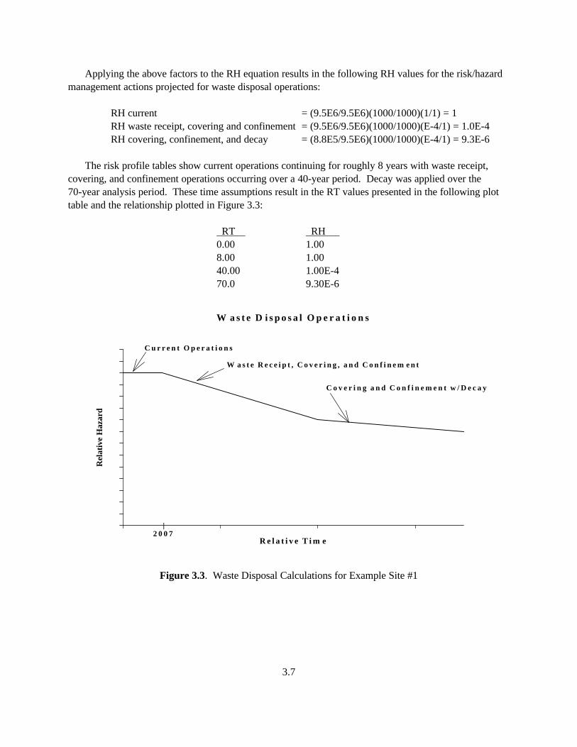
3.7

Applying the above factors to the RH equation results in the following RH values for the risk/hazardmanagement actions projected for waste disposal operations:

RH current = (9.5E6/9.5E6)(1000/1000)(1/1) = 1RH waste receipt, covering and confinement = (9.5E6/9.5E6)(1000/1000)(E-4/1) = 1.0E-4RH covering, confinement, and decay = (8.8E5/9.5E6)(1000/1000)(E-4/1) = 9.3E-6

The risk profile tables show current operations continuing for roughly 8 years with waste receipt,covering, and confinement operations occurring over a 40-year period. Decay was applied over the70-year analysis period. These time assumptions result in the RT values presented in the following plottable and the relationship plotted in Figure 3.3:

RT RH 0.00 1.008.00 1.0040.00 1.00E-470.0 9.30E-6

W a s t e D i s p o s a l O p e r a t i o n s


Rel

ativ

e H

azar

d

C u r r e n t O p e r a t i o n s

W a s t e R e c e i p t , C o v e r i n g , a n d C o n f i n e m e n t

C o v e r i n g a n d C o n f i n e m e n t w / D e c a y

|2 0 0 7

Figure 3.3. Waste Disposal Calculations for Example Site #1

3.8

3.1.4 References

Since the purpose of this analysis is only to serve as an example, the pertinent references are notincluded; however, documenting the references is an important part of an actual analysis. In pastanalyses, the inventory information was assembled in a spreadsheet utilizing the reference note capabilityof the spreadsheet software. This allows documentation of the references from which each specific pieceof information/data was obtained. It is also good practice to include a bibliographic list of all thereferences (cited in the spreadsheet) in the calculation notes.

3.2 Example Site #2

The Example Site #2 analysis provides a good example of a site with detailed annual source-termquantity data. However, for security reasons, detailed curie-content data were not releasable for all wastetypes at the site. Thus, the volume data were used in the analysis. These data are less desirable for theanalysis because the results will be less comparable across the different waste types. It also necessitatesassigning the entire volume of the material to the controlling constituent quantity. This generallyproduces an overly conservative quantity of the respective constituents. However, since the RH is a ratio,these quantities will balance out for most cases. This overly conservative approach could greatly impactthe relative hazard results when risk management actions involve direct modification of part or all of theinventory (e.g, separation, elimination, or reduction of controlling constituents in the total inventory).

The inventories were taken from the site’s disposition maps. Specific waste streams within a wastetype were consolidated in an effort to roll up the inventories to the highest level that matched the PBSdescriptions. Hazard control factors were based on risk evaluations conducted for a site-specificcumulative impact assessment.

3.2.1 Nuclear Materials Calculation Notes

The air pathway is assumed to be the controlling pathway.

The initial inventory is the sum of the inventories presented for nuclear materials in the risk profiletables, divided into the categories of solids/sludges and liquids.

Q = 1.3E4 kg solids and sludgesQ = 1.2E2 kg liquids


RF = 1.0

The plutonium and uranium isotopes were considered to be the controlling constituents for theanalysis. Using the HM look-up table for the air pathway, an HM value of 1.0E4 was assigned.

HM = 1.0E4

3.9

Based on an internal risk assessment for the site, the site submitted the following HC values to beconsidered for the projected risk/hazard management actions:

HC current = 1 (baseline)HC solid residue stabilize and repack = 1.8 (reflects increase in inventory

activity)HC pits removed from site = 0.4HC special nuclear materials (SNM) consolidated = 0.1

HC enriched uranium removed from site = 0.05HC liquid residue stabilization = 0.01HC Pu metal and oxides stabilized, repacked and shipped offsite = 0.005HC solid residue stabilized, repacked and shipped offsite = 0.001


RH current solid and sludge = (1.3E4/1.3E4)(1/1)(1.0E4/1.0E4)(1/1) = 1RH current liquid = (1.2E2/1.2E2)(1/1)(1.0E4/1.0E4)(1/1) = 1RH solid residue stabilize and repack = (1.3E4/1.3E4)(1/1)(1.8/1) = 1.8RH pits removed from site (1.3E4/1.3E4)(1/1)(1.0E4/1.0E4)(0.4/1) = 0.4RH SNM consolidated = (1.3E4/1.3E4)(1/1)(1.0E4/1.0E4)(0.01/1) = 0.01RH enriched uranium removed from site = (1.3E4/1.3E4)(1/1)(1.0E4/1.0E4)(0.05/1) = 0.05RH liquid residue stabilization = (1.2E2/1.2E2)(1/1)(1.0E4/1.0E4)(0.1/1) = 0.1RH Pu metal and oxides stabilized, repacked, = (1.3E4/1.3E4)(1/1)and shipped offsite (1.0E4/1.0E4)(0.005/1) = 0.005RH solid residue stabilized, repacked and = (1.3E4/1.3E4)(1/1)

shipped offsite (1.0E4/1.0E4)(0.001/1) = 0.001

Only a 20-year analysis period was used because the site is schedule to be cleaned up within thatperiod of time. The site provided specific dates for completion of the various risk/hazard managementactivities, which were converted directly by starting from a 1998 starting point into the RT values shownin the following table and the plot in Figure 3.4:

RT RH0.00 1.001.00 1.001.50 1.801.55 0.401.70 0.103.50 5.00E-27.00 1.00E-27.80 5.00E-3

20.00 1.00E-3

3.10

N u c l e a r M a t e r i a l


Rel

ativ

e H

azar

d

C u r r e n t O p e r a t i o n sS o l i d R e s i d u e S t a b i l i z a t i o n & R e p a c k

P i t s R e m o v e d F r o m S i t e

S N M C o n s o l i d a t e d i n B 3 7 1

E n r i c h e d U r a n i u m ( e U ) R e m o v e d F r o m S i t e

L i q u i d R e s i d u e S t a b i l i z a t i o n C o m p l e t e

P u M e t a l s a n d O x i d e s S t a b i l i z e d ,R e p a c k e d a n d S h i p p e d O f f s i t e

S o l i d R e s i d u e S t a b i l i z e d ,R e p a c k a g e d a n d S h i p p e d O f f s i t e

Figure 3.4. Nuclear Material Relative Hazards Calculated for Example Site #2

3.2.2 Transuranic Waste Calculation Notes

The air pathway is assumed to be the controlling pathway.

The total inventory is the sum of the inventories presented for transuranic waste in the risk profiletables.

Q = 9.5E3 m3

The site provided the following year-by-year inventory projections through the year 2009, withrunning Q values assigned accordingly, which included each year’s increase:

Year Additional Inventory (m3)1998 1261999 10002000 20002001 20002002 20002003 17742004 3442005 1572006 642007 452008 142009 9

Total 9.5E3

3.11


RF = 1

The plutonium isotopes were considered to be the controlling constituents for the analysis. Using theHM look-up table for the air pathway, an HM value of 1.0E4 was assigned.

HM = 1.0E4


HC current = 1 (baseline)HC during residue stabilization and decontamination and decommissioning (D&D) activities

= 1 (actual increases in RH due to generation, shown as inventory increase)HC residue stabilization and D&D complete

= 0.0001


RH 1998 = (126/126)(1/1)(1.0E4/1.0E4)(1/1) = 1RH 1999 = [(126+1000)/126](1/1)(1.0E4/1.0E4)((1/1) = 8.9RH 2000 = [(126+1000+2000)/126](1/1)(1.0E4/1.0E4)(1/1) = 24.8RH 2001 = [(126+1000+2000+2000)/126](1/1)(1.0E4/1.0E4)(1/1) = 40.7RH 2002 = [(126+1000+2000+2000+2000)/126](1/1)(1.0E4/1.0E4)(1/1) = 56.6RH 2003 = [(126+1000+6000+1774)/126](1/1)(1.0E4/1.0E4)(1/1) = 70.6RH 2004 = [(126+1000+6000+1774+344)/126](1/1)(1.0E4/1.0E4)(1/1) = 73.3RH 2005 = [(126+1000+6000+1774+344+157)/126](1/1)(1.0E4/1.0E4)(1/1) = 74.6RH 2006 = [(126+1000+6000+1774+344+157+64)/126](1/1)(1.0E4/1.0E4)(1/1) = 75.1RH 2007 = [(126+1000+6000+1774+344+157+64+45)/126](1/1)(1.0E4/1.0E4)(1/1)

= 75.5RH 2008 = [(126+1000+6000+1774+344+157+64+45+14)/126](1/1)(1.0E4/1.0E4)(1/1)

= 75.6RH 2009 = [(126+1000+6000+1774+344+157+64+45+14+9)/126](1/1)(1.0E4/1.0E4)

(1/1) = 75.63RH residue stabilization and D&D complete

= (9533/126)(1/1)(1.0E4/1.0E4)(0.0001/1)= 7.5E-3

Only a 20-year analysis period was used because the site is scheduled to be cleaned up within thatperiod of time. The individual years associated with each inventory change were used to directly assignRT values, resulting in the following table and the plot in Figure 3.5:

3.12

RT RH

0.00 1.001.00 1.002.00 8.903.00 24.804.00 40.705.00 56.606.00 70.607.00 73.308.00 74.609.00 75.10

10.00 75.5011.00 75.6012.00 75.6316 0.007520.0 0.0075

T r a n s u r a n i c W a s t e


Rel

ativ

e H

azar

d

R e s i d u e S t a b i l i z a t i o n a n d D & D G e n e r a t i o n

R e s i d u e S t a b i l i z a t i o na n d D & D C o m p l e t i o n

Figure 3.5. Transuranic Waste Relative Hazards Calculated for Example Site #2

3.2.3 Low-Level Waste and Mixed Low-Level Waste Calculation Notes

The surface water pathway is assumed to be the controlling pathway.

The total inventory is the sum of the inventories presented for low-level waste (LLW) and mixed low-level waste (MLLW) in the risk profile tables.

3.13

Q = 3.5E5 m3

The site provided the following year-by-year inventory projections through the year 2020, withQ values for each year assigned accordingly:

Year Inventory (m3)1998 71181999 92502000 68002001 188992002 126352003 131492004 140432005 133092006 126472007 122342008 122242009 119772010 119772020 11977

Total 3.5E5


RF = 1

The plutonium and uranium isotopes were considered to be the controlling constituents for theanalysis. Using the HM look-up table for the surface water pathway, an HM value of 1.0E3 was assigned.

HM = 1.0E3 (Pu and U isotopes, 100 nCi/g controlling constituents)


HC current = 1 (baseline)HC D&D completion = 1.0E-3

Applying the above factors to the RH equation results in the following RH values for the risk/hazardmanagement actions projected for the site:

RH 1998 = (7118/7118)(1/1)(1.0E3/1.0E3)(1/1) = 1RH 1999 = (9250/7118)(1/1)(1.0E3/1.0E3)(1/1) = 1.3RH 2000 = (6800/7118)(1/1)(1.0E3/1.0E3)(1/1) = 0.96

3.14

RH 2001 = (18899/7118)(1/1)(1.0E3/1.0E3)(1/1) = 2.65RH 2002 = (12635/7118)(1/1)(1.0E3/1.0E3)(1/1) = 1.77RH 2003 = (13149/7118)(1/1)(1.0e3/1.0E3)(1/1) = 1.84RH 2004 = (14043/7118)(1/1)(1.0E3/1.0E3)(1/1) = 1.97RH 2005 = (13309/7118)(1/1)(1.0E3/1.0E3)(1/1) = 1.87RH 2006 = (12647/7118)(1/1)(1/0E3/1.0E3)(1/1) = 1.77RH 2007 = (12234/7118)(1/1)(1.0E3/1.0E3)(1/1) = 1.71RH 2008 = (12224/7118)(1/1)(1.0E3/1.0E3)(1/1) = 1.71RH 2009 = (11977/7118)(1/1)(1.0E3/1.0E3)(1/1) = 1.69RH 2010 = (11977/7118)(1/1)(1.0E3/1.0E3)(1.0E-3/1) = 1.69E-3RH 2020 = (11977/7118)(1/1)(1.0E3/1.0E3)(1.0E-3/1) = 1.69E-3

Only a 20-year analysis period was used because the site is scheduled to be cleaned up within thatperiod of time. The individual years associated with each inventory were used to directly assign RTvalues, resulting in the following table and the plot in Figure 3.6:

RT RH

0.00 1.001.00 1.002.00 1.303.00 0.964.00 2.655.00 1.776.00 1.847.00 1.978.00 1.879.00 1.77

10.00 1.7111.00 1.7112.00 1.6913.0 1.69E-323.0 1.69E-3

3.15

L o w L e v e l a n d L o w L e v e l M i x e d W a s t e


Rel

ativ

e H

azar

d

.

R a m p U p o f D & D

D & D O p e r a t i o n s

E n v i r o n m e n t a l R e s t o r a t i o n O p e r a t i o n s

D & C o m p l e t i o n

Figure 3.6. LLW and LLMW Relative Hazards Calculated for Example Site #2

4.1

4.0 Summary

The methodology presented in this document was developed to provide a means of calculating the RHratios to use in developing useful graphic illustrations. The RH equation, as presented in this method-ology, is primarily a collection of key factors relevant to understanding the hazards and risks associatedwith projected risk management activities. The RH equation has the potential for much broaderapplication than generating risk profiles. For example, it can be used to compare one risk managementactivity with another, instead of just comparing it to a fixed baseline as was done for the risk profiles. Ifthe appropriate source term data are available, it could be used in its non-ratio form to estimate absolutevalues of the associated hazards. These estimated values of hazard could then be examined to helpunderstand which risk management activities are addressing the higher hazard conditions at a site.Graphics could be generated from these absolute hazard values to compare high-hazard conditions. If theRH equation is used in this manner, care must be taken to specifically define and qualify the estimatedabsolute hazard values (e.g., identify which factors were considered and which ones tended to drive thehazard estimation).

5.1

5.0 References

40 CFR 302, U.S. Environmental Protection Agency, Designation of Hazardous Substances. 1989. Codeof Federal Regulations.

Buck, J.W., L.M. Bagaasen, M.P. Bergeron, G.P. Streile, L.H. Staven, K.J. Castleton, G.M. Gelston,D.L. Strenge, K.M. Krupka, R.J. Serne, and T.A. Ikenberry. 1997. Analysis of the Long-Term Impact ofTRU Waste Remaining at Generator Sites for No Action Alternative 2. PNL-11251, Pacific NorthwestNational Laboratory, Richland, Washington.

Droppo, J.G., Jr. D. L. Strenge, J. W. Buck, B. L. Hoopes, R.D. Brockhaus, M. B. Walter, and G. Whelan.1989. Multimedia Environmental Pollutant Assessment System (MEPAS) Application GuidanceVolume 1 – User’s Guide. PNL-7216, Pacific Northwest Laboratory, Richland, Washington.

Hawley, K.A., and B.A. Napier. 1985. A Ranking System for Mixed Radioactive and Hazardous WasteSites in U.S. DOE. Proceedings of the Fifth DOE Environmental Protection Information Meeting. CONF-841187, Volume 1. Proceedings of a conference held in Albuquerque, New Mexico, November 6-8,1984. U.S. Department of Energy, Washington, D.C.

Hawley, K.A., R.A. Peloquin, and R.D. Stenner. 1986. Modified Hazard Ranking System for Sites withMixed Radioactive and Hazardous Wastes – User Manual. PNL-5841, Pacific Northwest Laboratory,Richland, Washington.

Holdren, G.R., C.S. Glance, L.K. Berg, K. Kelinger, C.J. Fosmire, S.M. Goodwin, J.R. Rustad,R. Schalla, and J.A. Schramke. 1995. Environmental Settings for Selected U.S. Department of EnergyInstallations - Support Information for the Programmatic Environmental Impact Statement and theBaseline Management Report. PNNL-10550, Pacific Northwest National Laboratory, Richland,Washington.

International Commission on Radiological Protection (ICRP). 1959. Report of Committee II onPermissible Dose for Internal Radiation. International Commission on Radiological Protection,Publication 2, Pergamon Press, New York.

International Commission on Radiological Protection (ICRP). 1979. Limits for Intakes of Radionuclidesby Workers. International Commission on Radiological Protection, Publication 30, Pergamon Press,New York.

Napier, B.A., R.A. Peloquin, D.L. Strenge, and J.V. Ramsdell. 1988a. Conceptual Representation.Vol. 1, of GENII – The Hanford Environmental Radiation Dosimetry Software System. PNL-6584,Pacific Northwest Laboratory, Richland, Washington.

5.2

Napier, B.A., R.A. Peloquin, D.L. Strenge, and J.V. Ramsdell. 1988b. User’s Manual. Vol. 2, ofGENII – The Hanford Environmental Radiation Dosimetry Software System. PNL-6584, PacificNorthwest Laboratory, Richland, Washington.

Napier, B.A., R.A. Peloquin, D.L. Strenge, and J.V. Ramsdell. 1988c. Code Maintenance Manual.Vol. 3 GENII – The Hanford Environmental Radiation Dosimetry Software System. PNL-6584, PacificNorthwest Laboratory, Richland, Washington.

Pacific Northwest National Laboratory (PNNL). 1996. Remedial Action Assessment System (RAAS)Version 1.1. PNL-8751, Rev. 3, Pacific Northwest National Laboratory, Richland, Washington.

Serne, R.J., and M.I. Wood. 1990. Hanford Waste-Form Release and Sediment Interaction. PNL-7297,Pacific Northwest Laboratory, Richland, Washington.

Strenge, D.L., and S.R. Peterson. 1989. Chemical Data Base for the Multimedia EnvironmentalPollutant Assessment System (MEPAS), Version 1. PNL-7145, Pacific Northwest Laboratory, Richland,Washington.

Stenner, R.D., R.A. Peloquin, and K.A. Hawley. 1986. Modified Hazard Ranking System/HazardRanking System for Sites with Mixed Radioactive and Hazardous Wastes – Software Documentation.PNL-6066, Pacific Northwest Laboratory, Richland, Washington.

U.S. Department of Energy (DOE). 1998a. Richland Operations Office: Risk Prospectus – HanfordSite. U.S. Department of Energy, Center for Risk Excellence, Argonne, Illinois.

U.S. Department of Energy (DOE). 1998b. Nevada Operations Office: Human Health and Safety RiskSummary – Nevada Test Site and Off-Site Test Areas. U.S. Department of Energy, Center for RiskExcellence, Argonne, Illinois.

U.S. Department of Energy (DOE). 1998c. Rocky Flats Field Office: Risk Summary – Rocky FlatsEnvironmental Technology Site. U.S. Department of Energy, Center for Risk Excellence, Argonne,Illinois.

U.S. Department of Energy (DOE). 1998d. Savannah River Operations Office: Risk Summary –Savannah River Site. U.S. Department of Energy, Center for Risk Excellence, Argonne, Illinois.

U.S. Department of Energy (DOE). 1998e. Albuquerque Operations Office: Risk Summary – PantexPlant, Sandia National Laboratories and Los Alamos National Laboratory. U.S. Department of Energy,Center for Risk Excellence, Argonne, Illinois.

U.S. Environmental Protection Agency (EPA). 1982. Uncontrolled Hazardous Waste Site RankingSystem, Appendix A, Subpart H of the National Oil and Hazardous Substance Contingency Plan. U.S.Environmental Protection Agency, Federal Register 31219-31243 (July 16, 1982).

5.3

Warren, B.R., and D.L. Strenge. 1994. Multimedia-Modeling Environmental Database and Editor(MMEDE): User Manual. PNNL-11562, Pacific Northwest National Laboratory, Richland, Washington.

PNNL-12008Rev. 0

Distr.1

Distribution

No. ofCopies

OFFSITE

M. GilbertsonDOE-EMEM-52

No. ofCopies

ONSITE

52 Pacific Northwest National Laboratory

W. B. Andrews K7-10W. J. Martin K3-54R. D. Stenner (50) K3-54

Relative Hazard Calculation Methodology

Documents

Transcript of Relative Hazard Calculation Methodology