Relationship-specific investment and hold-up problems in ...

ORIGINAL RESEARCH

Relationship-specific investment and hold-up problemsin supply chains: theory and experiments

Ernan Haruvy1 • Elena Katok1 • Zhongwen Ma1 •

Suresh Sethi1

Received: 5 April 2018 / Accepted: 25 June 2018 / Published online: 20 July 2018

� The Author(s) 2018

Abstract Supply chains today routinely use third parties for many strategic

activities, such as manufacturing, R&D, or software development. These activities

often include relationship-specific investment on the part of the vendor, while final

outcomes can be uncertain. Therefore, writing complete contracts for such

arrangements is often not feasible, but incomplete contracts, especially when rela-

tionship-specific investment is required, may leave the supplier vulnerable to a

version of the ‘‘hold-up problem,’’ which is known to result in sub-optimal levels of

investment. We model the phenomenon as a sequential move game with asymmetric

information. Absent behavioral considerations, the unique Perfect Bayesian

Equilibrium implies zero investment. However, with social preferences, the hold-up

problem may be mitigated. We propose a model that incorporates social preferences

and random errors, and solve for the equilibrium. In addition, we look at reputation

and find it to be effective for increasing investment. We conduct laboratory

experiments with human subjects and find that a model with social preferences and

random errors organizes our data well.

Keywords Supply chain contracts � Behavioral economics � Game

theory

& Elena Katok

[email protected]

Ernan Haruvy

[email protected]

Zhongwen Ma

[email protected]

Suresh Sethi

[email protected]

1 Naveen Jindal School of Management, University of Texas at Dallas, Richardson, TX 75080,

USA

123

Business Research (2019) 12:45–74

https://doi.org/10.1007/s40685-018-0068-0

http://orcid.org/0000-0002-7037-7896

http://crossmark.crossref.org/dialog/?doi=10.1007/s40685-018-0068-0&domain=pdf

http://crossmark.crossref.org/dialog/?doi=10.1007/s40685-018-0068-0&domain=pdf

https://doi.org/10.1007/s40685-018-0068-0

1 Introduction

1.1 Theoretical and Empirical Background

Today, firms increasingly rely on third party vendors for many strategic activities,

including manufacturing. For example, The New York Times reported that

‘‘…almost all of the 70 million iPhones, 30 million iPads and 59 million other

products Apple sold last year were manufactured overseas.’’ (Duhigg and Bradsher

2012). Reliance on vendors for performing strategic activities, such as the

manufacturing of products using proprietary technology, creates a number of

pitfalls. One of the major pitfalls, and the focus of our paper, has to do with a

version of the hold-up problem.

The hold-up problem (Rogerson 1992) emerges when one firm in a relationship is

able to expropriate the returns from an investment made by another firm (for a

discussion on the ability of a firm to appropriate value, see MacDonald and Ryall

2004). Specifically, if one firm makes an investment that has a low value outside of

the relationship, that firm is vulnerable to being ‘‘held up’’ for the value of that

relationship-specific investment. The hold-up problem is particularly likely to

emerge in settings in which writing complete contracts is not feasible due to some

combination of information asymmetry and environmental uncertainty (Rogerson

1992). It has long been argued in the economics literature (see Coase 2006 for an

overview) that the presence of a potential hold-up problem results in under-

investment in relationship-specific investments leading to inefficiency, and so the

ability to mitigate the hold-up problem has potential value.

Crocker and Reynolds (1993) describe an interesting example from the 1970s

dealing with government procurement. The US military made a significant

investment in Research & Development (R&D) for production of jet engines for

F-15 and F-16 fighter. The military was working with Pratt & Whitney as a sole

source supplier on this project. As the sole supplier, Pratt was in a strong position to

hold up the US military by demanding excessive concessions to correct quality

problems. As a result, in 1979 the Air Force commissioned General Electric to

develop a functionally equivalent jet engine for the use in its B-1 bomber. This

resolved the hold-up problem and the number of contract disputes decreased, but at

the cost of funding a second engine by the US Military. The US Congress has

continued to fund the two engines through 2011 (Schone 2011).

Other examples of negative and costly consequences that have the hold-up flavor

include expensive and protracted lawsuits, such as one between the U.S. Postal

Service and Northrop–Grumman Corp., whose contract dispute led to over $500

million in lawsuits (Reilly 2012). Fears of the hold-up problem, on the other hand,

result in under-investment by suppliers (Haruvy et al. 2012), leading to Original

Equipment Manufacturers (OEMs) being unable to fill lucrative contracts. Barnes

(2012) describes Boeing’s situation of being unable to fill orders worth billions of

dollars for many years due to its suppliers’ inability or unwillingness to invest in

required capacity.

46 Business Research (2019) 12:45–74

123

1.2 Experimental literature on the hold-up problem

We study incomplete contracts that make one of the players vulnerable to a version

of the hold-up problem, using laboratory experiments with human subjects. In the

experimental economics literature, the hold-up problem builds on the extensively

studied investment game (Berg et al. 1995). In the investment game, the first

mover—the seller (the terms seller and buyer are accepted terminology, e.g., Hoppe

and Schmitz 2011)—decides whether to invest in production. Investment creates

surplus (generally in investment game experiments, the surplus to be divided is

three times the investment amount—a parameterization not required for the

definition of an investment game). The second mover—the buyer—decides how

much of the created surplus to expropriate. There is much room for mutual gain of

both parties, but given the sequential nature of the game, it is best response of the

buyer to expropriate the entire surplus in a single shot game. By backward

induction, the seller will not invest. In numerous experimental studies (see overview

in Camerer 2003), the general pattern is that sellers do invest and buyers share some

of the surplus with the sellers.

The setting that we study in this paper is different from the standard investment

game in several aspects. One aspect is that the seller has the last word and can

accept or reject the buyer’s offer. In Dufwenberg et al. (2013), two variations were

studied. In the first, the ‘‘Low game,’’ the first mover could reject an unkind surplus

division, resulting in a loss to both himself and the second mover. In the second, the

‘‘High game,’’ rejection would actually improve the outcome for the buyer, and thus

may not be useful as a threat. As expected, none of the sellers who decided to

initially produce chose to reject an unkind offer that results in a gain to the buyer.

Even in this High game version, there is investment (40%) by the seller, which is

difficult to justify in an equilibrium sense. The authors also report that the vast

majority of buyers (90%) in fact did choose the unkind surplus division, which

makes the fact that 40% of the sellers chose to invest particularly surprising.

Ellingsen and Johannesson (2004a) run a hold-up game experiment as well (using

the term hold-up), to study the effect of communication. Their interpretation of what

constitutes a hold-up game is the same as Dufwenberg et al. The seller (their

terminology has seller and buyer) first decides whether to invest 60 or not. Then, the

buyer proposes a division of 100 tokens, which is the revenue created by the

investment. The seller can then accept or reject. This structure is the same as

Dufwenberg et al. with somewhat different payoffs. The purpose of the experiment

was to compare the basic treatment to communication treatments with promises by

the buyers or threats by the seller. They found that communication did in fact

mitigate the hold-up problem. An important companion to Ellingsen and Johan-

nesson (2004a) is Ellingsen and Johannesson (2004b). A key difference between

these two studies is that bargaining in the latter is not in ultimatum format. In that

design, each of the two agents makes a claim. The revenue is equal to 0 if the sum of

the claims exceeds 100. If the sum of the claims is 100 or less, each subject gets his

claim (i.e., bilateral bargaining according to Nash’s demand game, Nash 1953).

Other than that, the experimental designs are largely identical. Ellingsen and

Johannesson (2004a) find that communication mitigates the hold-up problem.

Business Research (2019) 12:45–74 47

123

Specifically, unilateral communication—by buyer or seller—facilitates coordination

and increases investment.

Hoppe and Schmitz (2011) study the effect of contracting on the hold-up game.

They find that option contracts improve performance. Unlike Dufwenberg, they add

a participation decision in which either party can decide to decline participating in

the game. After that stage, the game has the same structure as Dufwenberg et al.

(2013): The seller makes an investment decision (0 or 8). The buyer then learns the

investment decision and makes a take-it-or-leave-it price offer. The seller can then

take it or leave it. If he leaves it, he forgoes the cost of the investment—thus the

hold-up. Hoppe and Schmitz model all contract decisions as eliminating one of the

stages and thus reducing the hold-up problem to an investment problem. In the fixed

price contract, the buyer’s pricing decision and the seller’s final accept/reject

decisions go away and the problem becomes equivalent to an investment/trust game

with the buyer moving first, choosing to pay the seller or not. If he pays, he has to

trust the seller to make the investment and not to expropriate the surplus. In the

option contract, the seller invests without the option of accepting or rejecting. They

also investigated a contract with renegotiation which is similar in spirit to the

communication study of Ellingsen and Johannesson (2004a) described above.

Davis and Leider (2013), similar to Hoppe and Schmitz (2011), study the

possibility that an option contract mitigates the holdup problem. In the option

contract, the retailer and supplier agree ex ante to buy and sell units up to D units at

a wholesale price of w and the retailer pays a lump sum option fee to the supplier.

The framework is different in that the first mover makes a capacity investment,

demand is random, and bargaining is structured. Bargaining is such that both roles

have the ability to make multiple back-and-forth offers while also providing

feedback on the offers they receive. They find that the option contract does indeed

mitigate the hold-up problem. They further find that the evolution of offers during

bargaining suggests ‘‘superficial fairness.’’ Specifically, wholesale price falls in the

middle of the available contracting space, away from the coordinating contract

parameter.

There are other studies that model settings that are closer to the theoretical hold-

up problem, without invoking the term. In Hackett (1994) experiment, for example,

two players decide on respective investments that increase joint surplus but also

increase individual cost. They then realize a probabilistic outcome that depends on

the investments and then bargain over the joint surplus, with either party having a

veto power. Hackett (1994) finds that the surplus division is responsive to the

investments. The setting is closer to the theoretical literature in that the unknown

realization of the eventual outcome makes the contract incomplete—unlike the

settings of Dufwenberg et al. (2013) and Hoppe and Schmitz (2011).

The key innovation in the setting we study, that distinguishes it from the

literature we summarized above, is the presence of asymmetric information.

Asymmetric information makes designing a ‘‘better contract’’ less plausible because

contingent contracts may be impossible to enforce. So the asymmetric information

aspect in our study is important for practice, and new in terms of research focus.


123

1.3 Behavioral contribution

It has been shown in experimental economics, as well as in the behavioral

operation management literature, that people are not motivated exclusively by

monetary payoffs—they have social preferences (see Cooper and Kagel 2015;

Loch and Wu 2008; Katok and Pavlov 2013). A stream of theoretical works

investigates social preferences, such as inequality aversion, in the context of the

hold-up problem (Gantner et al. 1998, Oosterbeek et al. 1999; Sonnemans et al.

2001; von Siemens 2009). Dufwenberg et al. (2013) argue that the patterns

observed in the hold-up problem are explained by reciprocity. We use a

behavioral model to analyze the hold-up problem, but our behavioral model uses

inequality aversion (Bolton and Ockenfels 2000; Fehr and Schmidt 1999; Cui

et al. 2007). We further solve the problem in a dynamic framework, whereas

Dufwenberg et al. (2013) analyze the one-shot setting. We analyze the dynamics

by approximating a dynamic setting in our experiments and refer to this as

dynamic approximation.

Thus, our solution concept involves a tradeoff. On the one hand, it is quite broad,

which allows us to use it for testing a model that does not rely on reciprocity

preferences and generalizing the solution to dynamic environments. On the other

hand, our approach involves an approximation that captures how people think about

the uncertain future actions of others. We think this approximation is reasonable and

is a good first step to understanding behavior in repeated settings.

Our second behavioral contribution is a demonstration that reputation

information can help solve the hold-up problem. Reputation may serve in lieu

of informal agreements (Hart et al. 2013). Board (2011) shows that theoretically,

even in the presence of many potential partners, an optimal contract design

implies loyalty to existing partners.1 Bolton et al. (2004) show that reputation

increases both trust and trustworthiness. They also report that, contrary to standard

theory, some cooperation exists even without a formal feedback mechanism. This

argument is also consistent with the findings by Ozer et al. (2011) that people are

more truthful than the standard theory predicts. Ozer et al. (2013) refine these

findings and extend them to a multi-cultural setting. Our work complements these

earlier findings by showing that some cooperation is consistent with the dynamic

equilibrium approximation in a repeated setting with a finite number of players.

More importantly, we show that even though the dynamic approximation analysis

is only an approximation for the actual setting in our experiment, it predicts the

outcomes remarkably well.

1 The proof hinges on grim-trigger punishment in an infinitely repeated game. Once a partner defects,

investment is zero forever after a certain period. The setting is not at all like ours because the principal

has multiple partners to choose from, and a rich space of repeated game strategies to employ, but the idea

of the game being more than a one-shot is an important component of the present setting, as well as the

concept of reputation.


123

2 Model

In this section, we describe the basic game setting used in our study. We show that if

players are motivated exclusively by monetary payoffs, the hold-up problem is

severe. We then proceed to extend the model to include social preferences and

random errors, and develop the dynamic equilibrium approximation that can predict

that these behavioral considerations may mitigate the hold-up problem.

2.1 The game and standard model

We begin with the basic setting, which is a sequential game with asymmetric

information. The standard analysis assumes that players care exclusively about their

monetary payoffs. We then proceed to add social preferences and random errors.

Figure 1 displays the extensive form of the game we analyze.

The seller moves first and decides whether to produce or not produce. If the seller

chooses not to produce, then the buyer and the seller earn their outside option

payoffs eB and eS, respectively. If the seller chooses to produce, product quality is

qL with probability d ¼ P qLð Þ and qH with probability 1� d ¼ P qHð Þ ¼ 1� P qLð Þ:Quality is privately known to the buyer.2 That is, the seller does not know the

quality while the buyer does. In the context of the buyer being an end consumer, this

is a straightforward assumption. The end consumer knows whether he likes the

product and finds it esthetically pleasing, functional, fitting, or satisfying. The seller

does his best to satisfy the consumer but if the consumer claims to be dissatisfied the

seller cannot verify whether this claim is correct. In a supply chain context, this

motivation extends to downstream channel members. The closer a channel member

is to the end consumer, the more knowledge he has regarding end customer

Fig. 1 Extensive form game

2 In the experiment, the buyer is told realized quality.


123

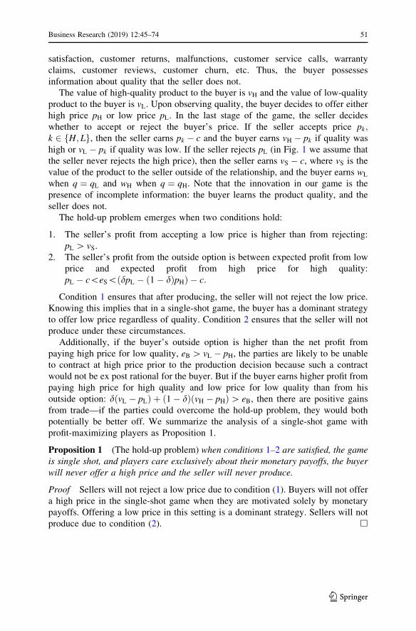
satisfaction, customer returns, malfunctions, customer service calls, warranty

claims, customer reviews, customer churn, etc. Thus, the buyer possesses

information about quality that the seller does not.

The value of high-quality product to the buyer is vH and the value of low-quality

product to the buyer is vL. Upon observing quality, the buyer decides to offer either

high price pH or low price pL. In the last stage of the game, the seller decides

whether to accept or reject the buyer’s price. If the seller accepts price pk;k 2 H; Lf g, then the seller earns pk � c and the buyer earns vH � pk if quality was

high or vL � pk if quality was low. If the seller rejects pL (in Fig. 1 we assume that

the seller never rejects the high price), then the seller earns vS � c, where vS is the

value of the product to the seller outside of the relationship, and the buyer earns wL

when q ¼ qL and wH when q ¼ qH. Note that the innovation in our game is the

presence of incomplete information: the buyer learns the product quality, and the

seller does not.

The hold-up problem emerges when two conditions hold:

1. The seller’s profit from accepting a low price is higher than from rejecting:

pL [ vS.

2. The seller’s profit from the outside option is between expected profit from low

price and expected profit from high price for high quality:

pL � c\eS\ dpL � 1� dð ÞpHð Þ � c:

Condition 1 ensures that after producing, the seller will not reject the low price.

Knowing this implies that in a single-shot game, the buyer has a dominant strategy

to offer low price regardless of quality. Condition 2 ensures that the seller will not

produce under these circumstances.

Additionally, if the buyer’s outside option is higher than the net profit from

paying high price for low quality, eB [ vL � pH, the parties are likely to be unable

to contract at high price prior to the production decision because such a contract

would not be ex post rational for the buyer. But if the buyer earns higher profit from

paying high price for high quality and low price for low quality than from his

outside option: d vL � pLð Þ þ 1� dð Þ vH � pHð Þ[ eB, then there are positive gains

from trade—if the parties could overcome the hold-up problem, they would both

potentially be better off. We summarize the analysis of a single-shot game with

profit-maximizing players as Proposition 1.

Proposition 1 (The hold-up problem) when conditions 1–2 are satisfied, the game

is single shot, and players care exclusively about their monetary payoffs, the buyer

will never offer a high price and the seller will never produce.

Proof Sellers will not reject a low price due to condition (1). Buyers will not offer

a high price in the single-shot game when they are motivated solely by monetary

payoffs. Offering a low price in this setting is a dominant strategy. Sellers will not

produce due to condition (2). h


123

2.2 Social preferences

We will apply to the game in Fig. 1 a simplified version of the inequality aversion

model by Bolton and Ockenfels (2000) that has been extended to a supply channel

setting by Cui et al. (2007).

Consider a linear version of the Bolton and Ockenfels (2000) and Fehr and

Schmidt (1999) model in which player i derives negative utility when her profit is

below some fair outcome in terms of the relative difference between her and player

j’s profit. Player i’s utility can be written as:

ui ¼ pi � a cpj � pi

� �þ�b pi � cpj

� �þ; ð1Þ

where a is player i’s degree of disadvantageous inequality aversion (negative utility

from earning less than some relative fair share c), and b is i’s degree of advanta-

geous inequality aversion. Parameter c represents the share of the channel profit thatplayer j earns under profit distribution that is considered to be fair (c may reflect

differences in initial investment or other value-added activities; see Cui et al. 2007).

In the rest of the paper, we will set c ¼ 1 because it is reasonable for our

laboratory setting and will simplify notation. For the same reasons, we will also

make the simplifying assumption b ¼ 0. The assumption of c ¼ 1 means that player

i considers the fair allocation to be at the point where the profits of both players are

exactly equal. Cui and Mallucci (2016) experimentally evaluated an environment

structured similarly to ours in that there is a two-stage dyadic channel, in which

firms decide on investments in the first stage and then on prices in the second stage.

Their utility specification is identical to our utility Eq. (1), with only a slight

notation difference. Specifically, they denote s= 1� sð Þ for our c. They note that

s ¼ 12(c = 1 in our notation) corresponds to the strict egalitarian ideal.

They also proposed a ‘‘sequence-aligned’’ notion of fairness in their framework

which corresponds to the share of the decision maker in their framework under the

Stackelberg equilibrium. In their setting, this notion prescribed s ¼ 13. In our

experiment, the equilibrium is for no production to take place, and both players earn

equal outside payoffs of 2, resulting in a sequence-aligned prescription of s ¼ 12

(c = 1 in our notation), identical to the egalitarian notion. Our study thus does not

distinguish these fairness notions, as they both prescribe c = 1.

Incidentally, Cui and Mallucci (2016) found that the sequence-aligned notion of

fairness fits their data better than the strict egalitarian value, and this is consistent

with c = 1 in our framework. They also conclude that b = 0 which we rely on as

support for our own b = 0 assumption.

The simplified seller’s utility function then becomes

uS ¼ pS � a pS � pBð Þþ;

and it will be used in the rest of the paper.

The main effect of inequality aversion on the seller has to do with the seller’s

reaction to low price. With inequality aversion, the seller needs to form a belief

about the buyer’s payoff, meaning that he has to form a belief about quality which

he does not observe. Specifically, the seller does not know quality realization but


123

can form a belief about quality conditional on the price he was offered. The critical

piece of information that the seller would like to know when he is offered a low

price is whether this was due to low quality or not. In other words, the seller would

like to know PðqLjpLÞ. We assume that the seller knows the unconditional

probability of being offered a high price, P pHð Þ (for example, based on historical

data), and then uses Bayes’ rule to calculate conditional probabilities. We further

assume that high price for low quality is dominated for the buyer so that

P pHjqLð Þ ¼ 0). This gives us

P qLjpLð Þ ¼ P pLjqLð ÞP qLð ÞP pLð Þ ¼ P qLð Þ

P pLð Þ ¼d

1� P pHð Þ : ð2Þ

We assume that the seller operates in the environment of being subject to

disadvantageous inequality only. The seller’s expected utilities from accepting and

rejecting a low price are

E uS pL;Að Þ½ � ¼ pL � c � a 1� d1� P pHð Þ

� �vH � pLð Þ þ d

1� P pHð Þ

� �vL � pLð Þ � ðpL � cÞ

� �þ;

E uS pL;Rð Þ½ � ¼ vS � c � a 1� d1� P pHð Þ

� �wH þ d

1� P pHð Þ

� �wL � vS � cð Þ

� �þ:

ð3Þ

Consider the terms in Eq. (3) that multiply a. These terms represent potential loss

in utility to the seller due to being relatively worse off than the buyer. If vS\pL

(according to Condition 1), which is a reasonable assumption for a setting in which

the seller makes a relationship-specific investment, then rejecting a low price makes

the seller worse off in absolute terms. If it is also the case that

1� d1� P pHð Þ

� �vH � pLð Þ þ d

1� P pHð Þ

� �vL � pLð Þ � ðpL � cÞ

� �þ

\ 1� d1� P pHð Þ

� �wH þ d

1� P pHð Þ

� �wL � vS � cð Þ

� �þ;

ð4Þ

then rejecting makes the seller worse off in relative terms as well, and consequently

the seller has no reason to reject, and the buyer can offer low prices with impunity.

We call (4) the impunity condition.

Proposition 2 (Reciprocity) If the impunity condition (4) does not hold and the

buyer earns higher profit from high price for high quality than from a rejection (

vH � pH [wH), the buyer motivated exclusively by profit may offer high price for

high quality in the single-shot game if the seller has sufficiently high a. A seller with

sufficiently high a will produce.

Proof If condition (4) does not hold, it means that there exists a high enough a thatthe seller with this a will have higher utility from rejecting than from accepting a

low price. Therefore, this seller may reject a low price. Since vH � pH [wH, the

buyer will offer high price for high quality. Since pH � c[ eS, the seller will

produce. h


123

2.3 Incorporating errors

It has been shown that laboratory participants make random errors (Su 2008). It is

useful to incorporate these random errors into the analysis to obtain better estimates

of behavioral parameters. We follow the basic idea of a logistic mapping between

expected utilities and action probabilities (e.g., McKelvey and Palfrey 1995). It

implies that people are more likely to choose an action that yields higher expected

utility.

Our goal here is to construct a parsimonious model that captures the essential

aspects of the problem setting. The critical aspects of the problem setting are the

ones that result in the hold-up problems: (1) the seller is financially better off to not

produce unless there is a sufficient likelihood that the buyer will offer high price for

high quality, and (2) in the long run, the buyer is much better off if the seller

produces, even if he has to induce production by sometimes paying high prices for

high quality. So the buyer and the seller face fundamentally different problems.

The seller will only produce if he expects to see a high price with sufficiently

high probability. It is reasonable to model a seller as if he is playing a game in

which he is using information from past rounds to forecast the probability P pHð Þ butis not attempting to affect the future behavior of the buyers. In contrast, the buyer is

facing a clear tradeoff each period between the immediate payoff from paying low

price for high quality and the loss from lack of production by suppliers in future

rounds. Therefore, we approximate buyers’ behavior with a model in which buyers

decide on a fixed probability of offering high price for high quality given the sellers’

response function and the behavior of other buyers in the market.3 That is, sellers

need to form beliefs given the history of the game, whereas buyers need to develop

reputations (individually or as a group) to make it desirable for sellers to produce.

This framework results in simple theoretical benchmarks that capture most of the

regularities of the data in our laboratory experiments.

2.3.1 The sellers

We model the seller’s probability of producing as a logit function (McKelvey and

Palfrey 1995).4

P Produceð Þ ¼ exp sE uS Produceð Þ½ �ð Þexp seSð Þ þ exp sE uS Produceð Þ½ �ð Þ ; ð5Þ

where s is the rationality parameter and

3 The model of buyers we propose is parsimonious, and we do not argue that it is ‘‘the right model’’ but

merely a very simple one that has a chance of being consistent with the data. For example, Ozer, Zheng

and Chen (2011) propose a model in which retailers, faced with a problem that has similar features to

ours, are averse to lying. Additionally, buyers could make random errors, which would not affect

qualitative predictions, but in all likelihood would make the model fit the data even better.4 In this section, we are analyzing the repeated game equilibrium approximation under the assumption

that sellers are ex ante symmetric, and therefore we do not subscript sellers’ decisions either by time

subscript t or seller subscript j. In the estimation section, in which we use the panel data from our

experiment, we will add subscripts for seller j and time period t to our notation.


123

E uS Pr oduceð Þ½ � ¼ P pHð ÞE uS pH;Að Þ½ �þ 1� P pHð Þð Þ P pL;Að ÞE uS pL;Að Þ½ � þ P pL;Rð ÞE uS pL;Rð Þ½ �½ �:

If the seller’s decision to reject is not dominated, then we start with the seller’s

decision to accept or reject a low price. The seller’s expected utility from accepting

a low or a high price works out to be

E uS pL;Að Þ½ � ¼ pL � c � a 1� d1� P pHð Þ

� �vH � vLð Þ þ vL � 2pL þ c

� �þ; ð6Þ

and

E uS pH;Að Þ½ � ¼ pH � c � a vH � 2pH þ cð Þþ:To keep the problem tractable, we assume vL � pL [ pL � c; meaning that the

term inside the parentheses in the expression for E uS pL;Að Þ½ � in Eq. (6) is positive.

Meanwhile, the seller’s expected utility from rejecting either a low or a high

price is

E uS pL;Rð Þ½ � ¼ E uS pH;Rð Þ½ � ¼ vS � c � a vB qð Þ � vS � cð Þð Þþ:

It follows that the probability of accepting price pk is

P pk;Að Þ ¼ exp sE uS pk;Að Þ½ �ð Þexp sE uS pk;Að Þ½ �ð Þ þ exp sE uS pk;Rð Þ½ �ð Þ ; k 2 H; Lf g: ð7Þ

2.3.2 The buyers

Let us assume that there are n buyers in the market, randomly matched with n

sellers, but the number of periods is large relative to n so that after some number of

periods, sellers assume that P pHð Þ in the current period will follow the probability

distribution of the past P pHð Þ. We assume full information, which means that P pHð Þforecasted by sellers, d ¼ P qLð Þ, as well as sellers’ a and s, are all known to buyers.

This means that buyers know (5) and (7)—the sellers’ probabilities of future

production and of rejecting a low price.

Each buyer i maximizes her expected long run average profit by choosing

Pi pHjqð Þ where q 2 qL; qHf g.max

PiðpHjqÞE uB Pi pHjqð Þð Þ½ � ð8Þ

where

E uB Pi pHjqð Þð Þ½ � ¼ P Produceð Þ dE uB Pi pHjqLð Þð Þ½ � þ 1� dð ÞE uB Pi pHjqHð Þð Þ½ �f gþ 1� P Produceð Þð ÞeB;

and P Produceð Þ is defined by (5) and in the long run depends on P pHð Þ observed by

the seller. Note that P pHð Þ is based on the behavior of all n buyers, so each buyer i

has an effect on the average P pHð Þ that a seller observes.

If the buyer never pays high price for low quality, so Pi pHjqLð Þ ¼ 0, then the

buyer’s expected utility when he observes low quality is


123

E uB Pi pHjqLð Þð Þ½ � ¼ P pL;Að Þ vL � pLð Þ þ P pL;Rð Þ vB qLð Þð Þ:Let us also assume that sellers accept high prices with certainty, so the buyer’s

expected utility when he observes high quality and offers high price for it with

probability PiðpHjqHÞ isE uB Pi pHjqHð Þð Þ½ � ¼ Pi pHjqHð Þ vH � pHð Þ

þ 1� Pi pHjqHð Þð Þ P pL;Að Þ vH � pLð Þ þ P pL;Rð ÞwH½ �:The last piece of the model is the link between buyer i’s average probability of

offering high price for high quality, Pi pHjqHð Þ, and the seller’s forecasted

probability of being offered a high price, P pHð Þ.In the dynamic equilibrium approximation, let P�iðpHjqHÞ be the average

probability from the other n - 1 buyers in the market of offering high price for high

quality. In this case, let the average probability of high price that sellers observe be

P pHð Þ ¼ 1� dð Þ 1� kð ÞP�i pHjqHð Þ þ kPi pHjqHð Þð Þ; ð9Þ

where k is the effect buyer i has on the total probability of high price in the

population of buyers. So for example, in the impunity treatments, if sellers correctly

calculate the historical probability of high price, then k ¼ 1n, where n is the total

number of buyers. In the dynamic equilibrium approximation, sellers use (9) in (5)–

(7) when they make their production and acceptance decisions. The buyer solves (8)

to find her average equilibrium probability of offering high price for high quality.

Let buyer i’s average equilibrium probability of offering high price for high quality

when the other n - 1 buyers use P�iðpHjqHÞ beP�

i;�i pHjqHð Þ ¼ argmaxPiðpHjqHÞ

E uB Pi pHjqHð Þð Þ½ �: ð10Þ

2.3.3 Reputation

Consider a setting in which a seller, rather than observing the history P pHð Þ for theentire market, observes instead seller-specific history, Pi pHð Þ ¼ 1� dð ÞPiðpHjqHÞ,for the seller i with whom she is matched in the current period. This implies k ¼ 1,

and (9) becomes

P pHð Þ ¼ 1� dð ÞPi pHjqHð Þ: ð11ÞIn other words, Pi pHð Þ is buyer i’s reputation. Intuitively, as k increases, buyer

i benefits more from offering a high price for high quality because he captures more

of the future benefits.

Proposition 3 (Reputation) In the dynamic equilibrium approximation,

P�i;�i pHjqHð Þ increases in k.

Proof See Appendix A.

Corollary 1 P�i;�i pHjqHð Þ is higher when reputation information is available than

when it is not available.


123

Proof Follows from the fact that k is higher when reputation information is

available. h

In summary, P�i;�i pHjqHð Þ is increasing in k. Moreover, reputation information

increases its value.

3 Experimental design and hypotheses

3.1 Experimental design

We designed a laboratory setting in which the hold-up problem would be present in

the single-shot game (consistent with Proposition 1). In all experimental treatments,

we set parameters at d ¼ 0:2; eS ¼ eB ¼ 2; vH ¼ 14; vL ¼ 7; c ¼ 4; pH ¼ 9; vS ¼ 5,

and pL ¼ 5:5. This means that if the quality is high and the buyer offers a high price,

both players earn 5 (pB ¼ pS ¼ 5), if the quality is high and the buyer offers a low

price that the seller accepts, then pB ¼ 14� 5:5 ¼ 8:5 and pS ¼ 5:5� 4 ¼ 1:5. Ifthe quality is low and the buyer offers a high price that the seller accepts, then

pB ¼ 7� 9 ¼ �2 and pS ¼ 9� 4 ¼ 5. If the quality is low and the buyer offers a

low price that the seller accepts, then pB ¼ 7� 5:5 ¼ 1:5 and pS ¼ 5:5� 4 ¼ 1:5.If the seller rejects, then pS ¼ 5� 4 ¼ 1 in all treatments.

Our experimental treatments vary in the effects seller rejection have on the profit

of the buyer. In the impunity condition, we set wL ¼ 2 and wH ¼ 9, and in the

reciprocity condition, we set wL ¼ wH ¼ 1. Thus, if the seller rejects, then in the

impunity condition pB ¼ 9 if the quality is high and pB ¼ 2 if the quality is low

(making the seller worse off from rejecting in relative terms as well as in absolute

terms), while in the reciprocity condition pB ¼ 1 regardless of quality (so the seller

is worse off in absolute terms, but better off in relative terms). Figure 2 provides

experimental parameters in the extensive form of the game. See appendix for

experimental instructions.

Fig. 2 Extensive form representation of the game in the laboratory experiment


123

3.2 Experimental treatments

The experiment includes three treatments. In all treatments, we randomly assign

participants to buyer and seller roles when they arrive at the laboratory, and they

keep the roles for the duration of the session. Each treatment includes four sessions,

and each session includes four buyers and four sellers. Participants play the game

corresponding to one treatment (with payoffs corresponding to Fig. 2) for 100

rounds. They are randomly re-matched each round. In total, our experiment includes

96 participants. We pay participants a $5 show-up fee and an additional amount

proportional to their total profits earned in the experiment. Average earnings were

$26.68 for buyers and $18.78 for sellers. We recruited participants using ORSEE

recruitment system (Greiner 2004) and offered cash as the only incentive to

participate. We designed experimental software using zTree (Fischbacher 2007).

Our design examines the effect of social preferences by comparing impunity and

reciprocity conditions. Additionally, we test an intervention that we call reputation,

in which we keep track and show to the seller the average number of times the

current buyer offered a high price. In summary, our experiment includes the

following three treatments:

1. In the impunity treatment, participants have access to their own prior history that

includes past production decisions, the price offered (if production occurred), and

their own realized profits. The buyers have one additional piece of information

that sellers do not have—the realized quality for the current and all past periods.

2. In the reciprocity treatment, the payoffs are different from the impunity

treatment—the only difference being in the buyer’s payoff that results from

seller’s rejection. Participants have access to the same historical information as

in the impunity treatment.

3. In the reputation treatment, the payoffs are the same as in the impunity

condition. Historical information is different. Specifically, sellers see the

proportion of the time the buyer with whom the seller is matched during the

current period offered a high price; this buyer-specific history is shown to the

seller prior to making the production decision.

3.3 Theoretical predictions and hypotheses

In this section, we derive theoretical predictions for the behavior in the three

treatments.

3.3.1 The impunity treatment

In the impunity treatment, a buyer motivated exclusively by monetary payoff

derives his average equilibrium probability of offering high price for high quality

according to Eqs. (8) and (9).

Figure 3 plots the buyer’s equilibrium expected profit as a function of the

probability of offering high price for high quality for three levels of a(a ¼ 0; a ¼ 0:25 and a ¼ 1), and s ¼ 2 in Fig. 3a and lower levels of s in Fig. 3b.


123

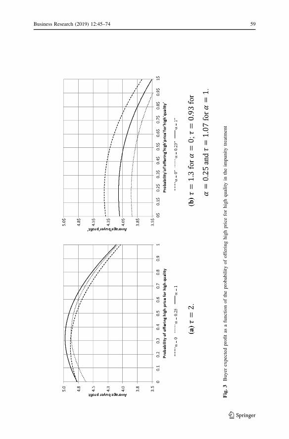
Fig.3

Buyer

expectedprofitas

afunctionoftheprobabilityofofferinghighprice

forhighqualityin

theim

punitytreatm

ent


123

It is easy to calculate that a fully rational seller (very high s) not concerned with

inequality aversion (a ¼ 0) prefers to produce as long as

P pHjqHð Þ[ 2�1:50:8 5�1:5ð Þ ¼ 0:1785, or equivalently P pHð Þ[ 0:1428. For a seller

concerned with inequality aversion, this threshold would be higher. A seller with

a low s, however, would produce even for a lower P pHð Þ.Figure 3a shows that when s ¼ 2 (this is the approximate level of swemeasured in

our data), buyer’s equilibrium P� pHð Þ ranges from 26% when a ¼ 0 to 36% when

a ¼ 0:25 (P� pHð Þ ¼ 0:32 for a ¼ 1). Figure 3b varies s for each level of a so as to

make P� pHjqHð Þ ¼ 0:1785: Here, s ranges from 0.93 for a ¼ 0:25 to 1.3 for a ¼ 0

(s ¼ 1:07 for a ¼ 1). Because those levels of s aremuch lower than the levels observed

in our data, our first hypothesis predicts positive levels of production and significant

probability of high prices given for high quality in the impunity treatment.

Hypothesis 1. In the impunity treatment, buyers offer high prices for high quality

on average at least 17.85% of the time, and sellers sometimes produce. Sellers never

reject any price offer.

Whether a seller produces depends on the seller’s a and on the P pHð Þ the seller

anticipates. The utility from not producing is 2, while the expected utility from

producing is

E uS Produceð Þ½ � ¼ 5P pHð Þ þ 1� P pHð Þð Þ 1:5� 7 1� d1� P pHð Þ

� �a

� �: ð12Þ

Setting E uS Produceð Þ½ � in Eq. (12) equal to 2 and solving for a characterizes

when a fully rational seller produces, i.e.,

a\5P pHð Þ þ 1:5 1� P pHð Þð Þ � 2

7 1� P pHð Þð Þ � d: ð13Þ

Note that since it is dominated for the buyer to offer a high price for low quality,

it follows that P pHð Þ� 1� d. Therefore, the closer P pHð Þ is to 1� d, the closer to

certainty it is for the seller to get high price for high quality and the more likely he is

to produce regardless of a. Generally, we see from (13) that for a fully rational

seller, the likelihood of production decreases in a and increases in P pHð Þ.

3.3.2 The reciprocity treatment

In the reciprocity treatment, rejection is not a dominated action for a seller because

even though the seller foregoes 0.5 in absolute profit, he implements the equal split.

The seller’s utility from rejecting a low price is 1, and based on Eq. (6), his expected

utility from accepting a low price is E uS pL;Að Þ½ � ¼ 1:5� 7a 1� d1�P pHð Þ

� , so a

fully rational seller whose a[ 0:57

1�P pHð Þ1�P pHð Þ�d

� would reject a low price. This gives

buyers an additional incentive to offer a high price for high quality in the reciprocity

treatment.

We plot the buyer’s expected profit function for three levels of a and s ¼ 2 in

Fig. 4. We see from the figure that P� pHð Þ is higher in the reciprocity treatment than


123

in the impunity treatment for all three levels of a, and the differences are especially

pronounced for higher values of a.We summarize predictions about the differences between the impunity and

reciprocity treatments in the following hypothesis:

Hypothesis 2. In the reciprocity treatment, the frequency of rejections of low

prices will be higher than in the impunity treatment, the frequency of high prices for

high quality will be higher than in the impunity treatment, and the production rate

will be higher than in the impunity treatment.

3.3.3 The reputation treatment

In the reputation treatment, we keep track of each buyer i’s proportion of high

prices, denoted Pi pHð Þ. We use the notation P pHð Þ to denote the average proportion

of high prices over the buyers in a cohort. In the reputation treatment, the seller

observes the buyer-specific Pi pHð Þ prior to deciding whether or not to produce.

Knowing Pi pHð Þ, the seller can use Eq. (5) to decide whether or not to produce for

each specific buyer. In the reputation treatment, each buyer controls his own Pi pHð Þ,in contrast to the impunity treatment, in which each buyer only affects the average

P pHð Þ in his group. Therefore, we expect higher proportion of high prices offered

for high quality in the reputation treatment than in the impunity treatment, and

indeed we can see from comparing Figs. 3a and 5 that P� pHð Þ is higher in the

reputation treatment than in the impunity treatment for all three levels of a. A higher

P� pHð Þ also implies a higher production rate in the reputation treatment than in the

impunity treatment, as we summarize in our last hypothesis.

Hypothesis 3 In the reputation treatment, production and high prices for high

quality will be higher than in the impunity treatment. Rejections will be similar

across the two treatments.

Fig. 4 Buyer’s expected profit as a function of the probability of offering high price for high quality inthe reciprocity treatment


123

4 Results

We present summary statistics for production, prices, profits and rejections in the

three treatments. We then report estimates for a behavioral model that includes non-

monetary preferences and errors.

4.1 Summary statistics

Table 1 reports average rates for production, high prices for high and low quality,

rejections and players’ earnings. We report standard errors in parenthesis, and we

use the session average as a unit of analysis (recall that each treatment includes four

sessions).

All p values reported are for a t test with four independent session-level

observations. We examine the results as they relate to H1 pertaining to the impunity

Fig. 5 Buyer’s expected profit as a function of the probability of offering high price for high quality inthe reputation treatment

Table 1 Summary statistics

Probability Treatment

Impunity Reciprocity Reputation

High prices for high quality 0.256 (0.090) 0.695 (0.177) 0.589 (0.083)

Production 0.569 (0.156) 0.821 (0.183) 0.771 (0.126)

Low prices rejected 0.140 (0.139) 0.527 (0.185) 0.105 (0.137)

High prices for low quality 0.075 (0.027) 0.003 (0.007) 0.103 (0.136)

High prices rejected 0.000 (0.000) 0.000 (0.000) 0.003 (0.004)

Seller earnings 2.154 (0.027) 3.205 (0.688) 2.909 (0.221)

Buyer earnings 4.523 (0.469) 3.848 (0.344) 4.401 (0.335)

Session is used as a unit of analysis. Each treatment incudes four sessions. Standard errors are in

parenthesis


123

treatment. As hypothesized, the proportion of high prices given for high quality is

significantly above zero in the impunity treatment (p = 0.010). In fact, the

proportion of high prices for high quality is not significantly different from the

hypothesized 0.1785 (p = 0.168), indicating that sellers with low a values are nearlyindifferent, on average, between producing and not producing. Last, as predicted,

the proportion of production is significantly above zero (p = 0.0053). These aspects

of the data are consistent with H1.

However, two aspects of the data are not entirely consistent with the theory. First,

the proportion of high prices given for low quality is low, but is significantly above

zero (p = 0.012). Second, the proportion of rejections is significantly above zero in

the impunity treatment (p = 0.011). However, both are sufficiently small in absolute

terms to be attributed to errors as we will show in the model estimation.

We now turn our attention to H2, concerned with the comparison of the impunity

and reciprocity treatments. We find that the data are consistent with H2 in that the

proportion of high prices given for high quality is significantly higher in the

reciprocity treatment than in the impunity treatment (p = 0.004), and the proportion

of production is higher in the reciprocity treatment than in the impunity treatment

(although only weakly significant; p = 0.080).

H3 is concerned with the comparison of the impunity and reputation treatments.

We find the patterns in the data to be consistent with H3. Specifically, the proportion

of high prices for high quality in the reputation treatment is above the corresponding

proportion in the impunity treatment (p = 0.002), and the proportion of production

in the reputation treatment is higher than the corresponding proportion in the

impunity treatment (weakly so; p = 0.086).

4.2 Dynamics

In Fig. 6, we present rejections, high prices offered for high quality, and production

rates, as they evolve over time. To focus on the trend, we aggregate 100 periods of

data into 20 five-period blocks. Rejections and production are highly stable after an

initial learning that takes about 20 periods. The proportion of high prices for high

quality is quite stable in rounds 21–80, but in the reputation treatment, in contrast to

the reciprocity treatment, it exhibits end-game effect in the last 20 rounds. This is

not surprising; other studies also found end-game effects in reputation treatments

(see for example Bolton et al. 2005).

In the next section, we report on estimation of a behavioral model using periods

21–100 for the analysis to eliminate the initial periods of steep learning.

4.3 Estimation

In this section, we jointly estimate behavioral parameters a and s for the behavioralmodel presented in Sect. 2.3. We estimate behavioral parameters for sellers only.

The buyers are assumed to anticipate seller’s reactions, and we capture their

decisions with a dynamic equilibrium approximation. Sellers make two decisions—

production and accept/reject—and these decisions are not independent. The

production decision of seller j in period t results in the probability of production


123

Fig.6

Averagerejections,pricesandproductionover

time


123

Pjt Produceð Þ, specified in Eq. (5) (but now indexed by j and t because we are using

panel data for estimation). This production decision depends, in turn, on the

probabilities of accepting price pk; k 2 L;Hf g; Pjt pk;Að Þ, the seller’s second

decision is determined by Eq. (7). Because the two decisions are not independent,

we estimate them jointly through a joint likelihood function.

Both of the seller’s decisions depend on the seller’s forecast of the buyer’s

conditional probability of paying a high price Pjit pHjqHð Þ, where i denotes the buyer

who has been matched with seller j in period t. We assume that in the impunity and

the reciprocity treatments, these forecasts are simply the average probability that

seller j observed high prices in the past, multiplied by the unconditional probability

of high quality. Specifically, in the estimation for impunity and reciprocity

treatments, Pjit pHjqHð Þ ¼ 1t�1

Pt�1s¼1 Pjs ¼ pH

� �. Note that subscript i does not appear

on the right hand side because the seller cannot distinguish among different buyers

in the impunity and the reciprocity treatments. In the reputation treatment, on the

other hand, the seller has historical information specific to buyer i:

Pjit pHjqHð Þ ¼ 1t�1

Pt�1s¼1 Pjis ¼ pH

� �:

The joint log-likelihood is defined as

LL ¼Xn

j¼1

XT

t¼1

ln Pjt Pr oduceð Þ� �

Pr oducejt þ ln 1� Pjt Produceð Þ� �

1� Producejt

� �

þ ln Pjt pjt;A� ��

Acceptjt þ ln 1� Pjt pjt;A� ��

1� Acceptjt� ��

;

where n is the total number of sellers in the session (n = 4), T is the number of

periods in a session (T = 100), Producejt is 1 if seller j decided to produce in period t

and 0 otherwise, and Acceptjt is 1 if seller j accepted the price the buyer offered in

period t and 0 otherwise.

The joint estimation implies that the parameter a is estimated in a way that

maximizes the fit not only of the acceptance/rejection decision but also of the

production decision. In the impunity and reputation treatments, where it is optimal

to always accept, one could expect that the production decision would have the

greater influence over the estimate of a, whereas in the reciprocity treatment, where

acceptance depends largely on inequality aversion, it would be the accept/reject

decision that would have the greater impact on the estimate.

We report results of the estimation in Table 2.

The main takeaway from the estimation has to do with the comparison between

predicted behavior, based on the estimates of a and s under the dynamic equilibrium

approximation analyzed in Sect. 2.35 (see bottom section of Table 2), and the actual

behavior (see Table 1). We stress that even though the dynamic equilibrium

approximation model in Sect. 2.3 is only a rough approximation for the actual

5 Predicted high prices for high quality are based on solving Eq. (10) for the impunity and reciprocity

treatments and Eq. (12) for the reputation treatment. Production probability is based on Eq. (5). Rejection

rates are based on Eq. (7). The average buyer’s and seller’s profits are also based on repeated game

equilibrium approximation solution given average behavioral parameters a and s.


123

setting, its prediction qualitatively matches virtually all important aspects of the

data:

1. Proportions of high prices for high quality and production rates are lowest in the

impunity treatment, highest in the reciprocity treatment, and in between in the

reputation treatment. None of the high price proportions are different from

predictions.

2. Proportions of low prices rejected are highest in the reciprocity treatment,

lowest in the reputation treatment, and in between in the impunity treatment.

None of the rejection rates are significantly different from predictions.

3. Seller profits are highest in the reciprocity treatment and lowest in the impunity

treatment. None of the seller’s profits are significantly different from

predictions.

4. Buyer’s profits are lowest in the impunity treatment. Buyer profits in the

impunity and reciprocity treatments are not significantly different from

predictions.

The only qualitative difference between predictions and the actual data is that

buyer’s profits are predicted to be higher in the reputation than in the impunity

treatment, while there is no statistically significant difference between them in the

data (p = 0.719). In fact, average buyer profits in the reputation treatment are

significantly lower than predicted (p = 0.031).

A deviation from predictions is that quantitatively the proportion of high prices

offered for high quality and production rates are slightly lower than predicted in the

reciprocity and reputation treatments. This may be due to individual heterogene-

ity—we computed predictions based on average values of a and s. In fact, there is a

good deal of heterogeneity in behavior (see Appendix B).

Table 2 Estimation results and predictions based on MLE

Impunity treatment Reciprocity treatment Reputation treatment

Fit

Log likelihood - 927.05 - 629.61 - 699.30

Parameters 3 3 3

v2 (restricted s) 13.068** 15.38** 4.19*

Estimated parameters

s Production 1.562** (0.029) 2.633** (0.141) 1.880** (0.131)

s Acceptance 2.342** (0.162) 1.435** (0.168) 1.564** (0.079)

a 0.042** (0.009) 0.102** (0.011) 0.042** (0.013)

Predictions| MLEs

High prices for high quality 0.260 0.763 0.510

Production 0.569 0.996 0.894

Rejection rate 0.253 0.446 0.188

Seller profit 2.285 4.115 3.191

Buyer profit 4.562 4.275 5.383

*p\ 0.05; **p\ 0.01


123

Last, inequality aversion appears low (although significant) in all three

treatments. The estimates are lower than estimates reported in the literature (for

example, De Bruyn and Bolton (2008) report a ¼ 1:03 in the linear version of the

model—of course they analyze bargaining games that are structurally quite different

from ours). In terms of our treatments, estimated a’s are not significantly different

between the impunity and reputation treatments (v2 ¼ 0:002; p ¼ 0:989) but are

significantly higher in the reciprocity treatment (v2 ¼ 15:51 for the comparison with

impunity and v2 ¼ 10:89 for the comparison with reputation; p\0:001 for both

comparisons). It is possible that inequality aversion is more salient in the reciprocity

treatment than in the other two treatments because the seller can implement a fair

split by punishing the buyer in that treatment. Saliency of inequality aversion is,

however, beyond the scope of this paper.

5 Conclusion

With the prevalence of using third party vendors for strategic activities, such as

manufacturing, by many major firms, the hold-up problem has to be considered as

one of the major pitfalls in supply chain management. For example, contract

manufacturers take on increasingly sophisticated tasks and activities requiring

relationship-specific investments which leave firms on both sides of the transaction

more vulnerable to the hold-up problem than ever before. Additionally, incomplete

information is typically present in these arrangements because the OEMs and

contract manufacturers are often located on different continents and are subject to

different cultural norms.

We analyze and test in the laboratory a stylized game designed to highlight the

possibility of the hold-up problem due to the relationship-specific investment by the

supplier. We derive approximate equilibrium predictions that match the data

remarkably well. In our impunity setting, the analysis predicts limited cooperation

but also a large loss in efficiency due to the hold-up problem—predictions that

match the data well. We also find, both analytically and empirically, that a setting in

which the supplier has the ability to negatively reciprocate, cooperation increases, as

does efficiency. Whether or not negative reciprocity is possible is usually not a

decision made by the parties but is rather a function of the environment, so we also

consider a setting in which we provide to the supplier basic reputation information

about the buyers’ past actions. We find that reputation information mitigates the

hold-up problem, both analytically and empirically.

The managerial implication of our work is that the hold-up problem can be

effectively mitigated in settings in which the relationship is not one shot. Most

supply chain relationships, even the ones that involve short-term contracts, are not

one shot, because information about the firm’s past actions tends to become

available to the community, even if informally. Our findings suggest that a

systematic way of making this reputation information available mitigates the hold-

up problem a great deal.


123

A fruitful direction for future research would be to test other, more sophisticated,

reputation system designs. For example, systems that track not just average

performance, but also provide information about recent versus past actions, may

work even better. It may also be worthwhile to analyze informal arrangements, such

as hand-shake agreements, in the context of relationship-specific investments, to

learn to what extent they may mitigate the hold-up problem.

Open Access This article is distributed under the terms of the Creative Commons Attribution 4.0

International License (http://creativecommons.org/licenses/by/4.0/), which permits unrestricted use, dis-

tribution, and reproduction in any medium, provided you give appropriate credit to the original

author(s) and the source, provide a link to theCreativeCommons license, and indicate if changesweremade.

Appendix A: Proof of Proposition 3

To find P�i;�i pHjqHð Þ, buyer i solves the optimization problem:

maxPi pHjqHð Þ

E uB Pi pHjqHð Þð Þ½ �

We assume that seller does not reject offers when it is dominated to do so in the

dynamic setting. Therefore, rejections do not depend on k or on Pi pHjqHð Þ).Rewriting the objective function for the optimization problem above and setting its

decision variable Pi pHjqHð Þ ¼ x gives

e YþZ 1�kð ÞP�i pHjqHð Þþxkð Þ½ �s

eeSs þ e YþZ 1�kð ÞP�i pHjqHð Þþxkð Þ½ �s

� vH � pHð Þx þ vH � pLð Þ 1� xð Þ 1� dð Þ½

þCd� vH � pHð Þxd� eB� þ 1;

ðA1Þ

where C, Y and Z are constants that we define to simplify the expressions:

Y ¼ pL � c � a 1� dð Þ vH � vLð Þ þ vL � 2pL þ cð Þð Þ;

Z ¼ pH � pL � a vH � 2pH þ cð Þþþa vH � 2pL þ cð Þ;

and C ¼ P pL;Að Þ vL � pLð Þ þ P pL;Rð Þ wLð Þ ¼ vL � pLð Þ.The first order condition (FOC) of expression (A1) with respect to decision

variable x is

vH � pHð Þ � vH � pLð Þð Þe YþZ 1�kð ÞP�i pHjqHð Þþxkð Þ½ �s 1� dð ÞþeeSs kZ Cd� eBð Þs� vH � pLð Þ 1� dð Þ 1� Z 1� xð Þskð Þ þ vH � pHð Þ 1� dð Þ 1þ Zxskð Þ½ �

�

e� YþZ 1�kð ÞP�i pHjqHð Þþxkð Þ½ �s eseS þ e YþZ 1�kð ÞP�i pHjqHð Þþxkð Þð Þsð Þ2

¼ 0:

Because the denominator is strictly positive, we restrict attention to the

numerator denoted as F �ð Þ:According to the implicit function theorem, x is increasing in k; iff

oxok ¼ � Fk

Fx[ 0:

We show that Fx is negative while Fk is positive for x�P�i pHjqHð Þ; whereFx ¼ eses þ es YþZ xkþP�i pHjqHð Þ�kP�i pHjqHð Þð Þð Þ� �

Z 1� dð Þks pL � pHð Þ;


123

http://creativecommons.org/licenses/by/4.0/

Fk ¼ Zses YþZ xkþP�i pHjqHð Þ�kP�i pHjqHð Þð Þð Þ pL � pHð Þ 1� dð Þ x � P�i pHjqHð Þð Þð Þþ Zseess dC þ x 1� dð Þ vH � pHð Þ þ 1� xð Þ 1� dð Þ vH � pLð Þ � ebf g:

Fx is negative because Z [ 0; pL\pH and 1� dð Þ[ 0:Since pL � pH\0 for x�P�i pHjqHð Þ, the Fp is positive if dC þ

x 1� dð Þ vH � pHð Þ þ 1� xð Þ 1� dð Þ vH � pLð Þ � eB [ 0: Because

� 1� xð Þ 1� dð Þ\0, therefore

�dC þ x �1þ dð Þ vH � pHð Þ þ �1þ x þ d� xdð Þ vH � pLð Þ þ eB\� dC

þ x �1þ dð Þ vH � pHð Þ þ �1þ x þ d� xdð Þ vH � pHð Þ þ eB

¼ �dC þ �1þ dð Þ vH � pHð Þ þ eB ¼ �d vL � pLð Þ þ �1þ dð Þ vH � pHð Þ þ eB

The above expression is negative, which follows from the assumption that

d vL � pLð Þ þ 1� dð Þ vH � pHð Þ[ eB in Sect. 2.1. We also checked the second order

condition of (A1) to verify that the solution of the optimization problem is a

maximum by showing that implicit function theorem when x�P�i pHjqHð Þ is

sufficient for the global maximum. h

Appendix B: Individual Heterogeneity

We calculated average P pHjqHð Þ and PðpHjqL) for the buyers, as well as average

production and rejection rates for the sellers. Figure 7 shows the distributions of

average P pHjqHð Þ and PðpHjqL) for individual buyers.

Figure 8 shows the distribution of average production rates for individual sellers.

Figure 9 shows the distribution of average rejection rates for individual sellers.


123

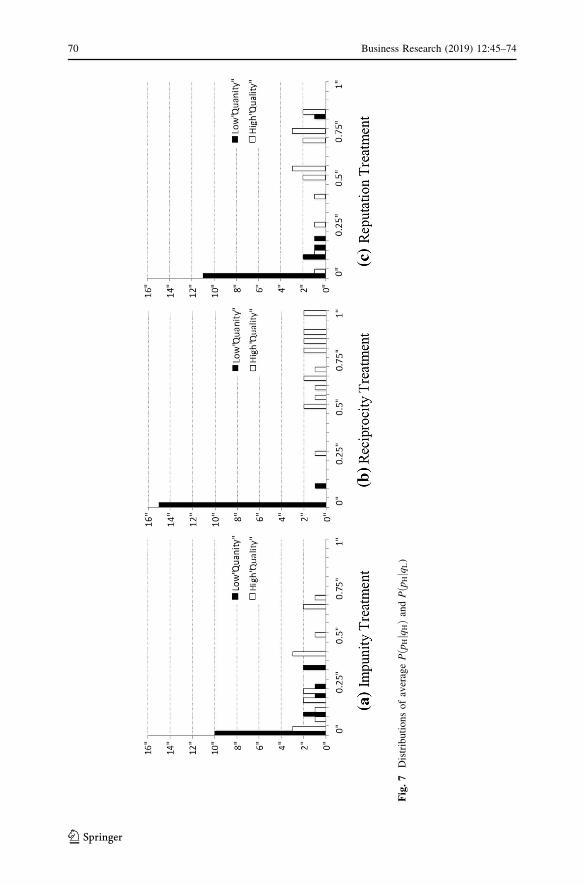
Fig.7

Distributionsofaverage

PpHjq

Hð

Þand

Pðp

Hjq

L)


123

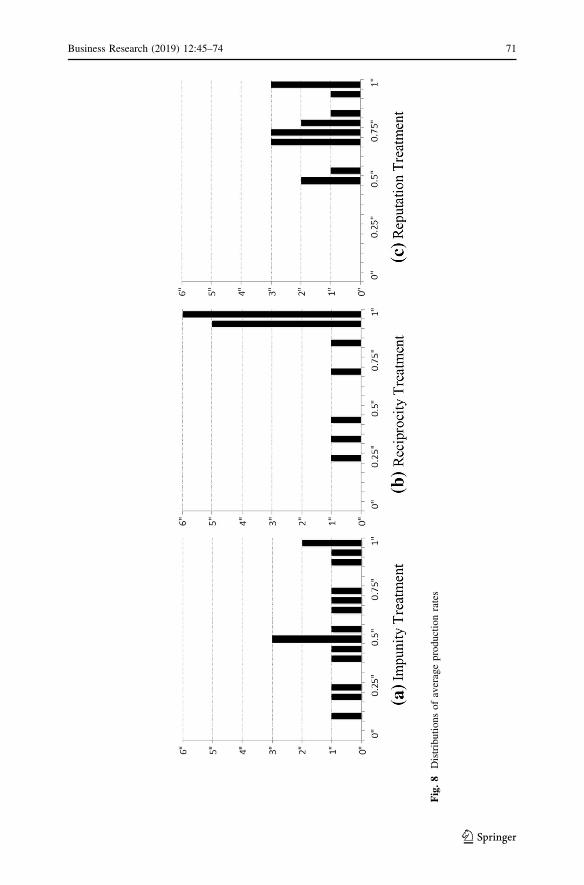
Fig.8

Distributionsofaverageproductionrates


123

Fig.9

Distributionsofaveragerejectionrates


123

References

Barnes, A, 2012 Boeing: Faster, faster, faster: The planemaker struggles to fulfill a rush of orders. The

Economist January 28, http://www.economist.com/node/21543555. Accessed 07/026/13.

Berg, Joyce, John Dickhaut, and Kevin McCabe. 1995. Trust, Reciprocity and Social History. Games and

Economic Behavior 10: 122–142.

Board, Simon. 2011. Relational Contracts and the Value of Loyalty. American Economic Review 101

((December 2011)): 3349–3367.

Bolton, G.E., and A. Ockenfels. 2000. A theory of equity, reciprocity, and competition. American

Economics Review 90 (1): 166–193.

Bolton, G.E., E. Katok, and A. Ockenfels. 2004. How effective are online reputation mechanisms? An

experimental study. Management Science 50 (11): 1587–1602.

Bolton, G.E., E. Katok, and A. Ockenfels. 2005. Cooperation among strangers with limited information

about reputation. Journal of Public Economics 89 (8): 1457–1468.

Camerer, Colin. 2003. Behavioral Game Theory: Experiments in Strategic Interaction. Princeton:

Princeton University Press.

Coase, R. 2006. The Conduct of Economics: The Example of Fisher Body and General Motors. Journal of

Economics & Management Strategy 15 (2): 255–278.

Cooper, D., and J. Kagel. 2015. Other Regarding Preferences: A Selective Survey of Experimental

Results. Forthcoming. In The Handbook of Experimental Economics 2, eds. Kagel, J., and A. Roth.

Princeton, NJ: Princeton University Press.

Crocker, K.J., and K.J. Reynolds. 1993. The Efficiency of Incomplete Contracts: An Empirical Analysis

of Air Force Engine Procurement. The RAND Journal of Economics 24 (1): 126–146.

Cui, T.H., J.S. Raju, and Z.J. Zhang. 2007. Fairness and channel coordination. Management Science 53

(8): 1303–1314.

Cui, Tony Haitao, and Paola Mallucci. 2016. Fairness Ideals in Distribution Channels. Journal of

Marketing Research 53 (6): 969–987.

Davis, Andrew and Stephen Leider (2013), Capacity Investment in Supply Chains Contracts and the

Hold-up Problem, working paper.

De Bruyn, A., and G.E. Bolton. 2008. Estimating the influence of fairness on bargaining behavior.

Management Science 54 (10): 1774–1791.

Dufwenberg, M., A. Smith, and M. Van Essen. 2013. Hold-up: with a Vengeance. Economic Inquiry 51:

896–908.

Duhigg C, Bradsher K (2012) How the U.S. Lost Out on iPhone Work. The New York Times, 1/21/2012.

http://www.nytimes.com/2012/01/22/business/apple-america-and-a-squeezed-middle-class.html?page

wanted=all&_r=0. Accessed 9 June 2013.

Ellingsen, T., and M. Johannesson. 2004a. Promises, Threats and Fairness. Economic Journal 114:

397–420.

Ellingsen, Tore, and Magnus Johannesson. 2004b. Is There a Hold-up Problem? Scandinavian Journal of

Economics 106 (3): 475–494.

Fehr, E., and K.M. Schmidt. 1999. A Theory of Fairness, Competition and Cooperation. Quarterly

Journal of Economics 114 (3): 817–868.

Fischbacher, U. 2007. z-Tree: Zurich Toolbox for Ready-made Economic experiments. Experimental

Economics 10 (2): 171–178.

Gantner A, W Guth, M Konigstein. 1998. Equity Anchoring in Simple Bargaining Games with

Production, Discussion paper 128, Department of Economics, Humboldt University

Greiner, B. 2004. An online recruitment system for economic experiments. In Forschung und

Wissenschaftliches Rechnen. GWDG Bericht 63, ed. K. Kremer, V. Macho Gottingen: Gesellschaft

fur Wissenschaftliche Datenverarbeitung, 79-93.

Hackett, S.C. 1994. Is Relational Exchange Possible in the Absence of Reputations and Repeated

Contact? Journal of Law Economics and Organization 10 (4): 360–389.

Hart O, E Fehr, C Zehnder 2013. Working paper. How Do Informal Agreements and Renegotiation Shape

Contractual Reference Points?.

Haruvy, E., T. Li, and S. Sethi. 2012. Two-Stage Pricing for Custom-Made Products. European Journal

of Operational Research 219 (2): 405–414.

Hoppe, E.I., and P.W. Schmitz. 2011. Can contracts solve the hold-up problem? Experimental evidence.

Games and Economic Behavior 73 (1): 186–199.


123

http://www.economist.com/node/21543555

http://www.nytimes.com/2012/01/22/business/apple-america-and-a-squeezed-middle-class.html%3fpagewanted%3dall%26_r%3d0

http://www.nytimes.com/2012/01/22/business/apple-america-and-a-squeezed-middle-class.html%3fpagewanted%3dall%26_r%3d0

Katok, E., and V. Pavlov. 2013. Fairness in supply chain contracts. Journal of Operations Management

31: 129–137.

Loch, C.H., and Y. Wu. 2008. Social preferences and supply chain performance: An experimental study.

Management Science 54 (11): 1835–1849.

MacDonald, G., and M.D. Ryall. 2004. How do value creation and competition determine whether a firm

appropriates value? Management Science 50 (10): 1319–1333.

McKelvey, R.D., and T.R. Palfrey. 1995. Quantal Response Equilibrium for Normal Form Games. Games

and Economic Behavior 10: 6–38.

Nash, J. 1953. Two-person Cooperative Games. Econometrica 21: 128–140.

Oosterbeek, H., J. Sonnemans, and S. van Velzen. 1999. Bargaining with Endogenous Pie Size and

Disagreement Points: A Holdup Experiment. Mimeo: University of Amsterdam.

Ozer, O., K. Zheng, and K. Chen. 2011. Trust in Forecast Information Sharing. Management Science 57

(6): 1111–1137.

Ozer O, K Zheng, Y Ren. 2013. Forecast Information Sharing in China and the U.S.: Country Effects in

Trust and Trustworthiness, Management Science forthcoming.

Reilly S. 2012. Northrop Grumman sues USPS in bitter contract dispute. Federal Times, May 8. http://

www.federaltimes.com/article/20120508/DEPARTMENTS02/205080307/Northrop-Grumman-sues-

USPS-bitter-contract-dispute. Accessed 07/026/13.

Rogerson, W. 1992. Contractual Solutions to the Hold-Up Problem. Review of Economic Studies 59 (4):

774–794.

Schone, M. 2011. After Work Stopped on Jet Engine, GE Blasts Competitor Pratt Whitney, ABC News,

3/25. http://abcnews.go.com/Blotter/work-stopped-jet-engine-ge-blasts-competitor-pratt/story?id=

13219559. Accessed 07/026/13.

Sonnemans, J., R. Sloof, and H. Oosterbeek. 2001. On the Relation between Asset Ownership and

Specific Investments. Economic Journal 111 (474): 791–820.

Su, X. 2008. Bounded rationality in newsvendor models. Manufacturing & Service Operations

Management 10 (4): 566–589.

von Siemens, F.A. 2009. Bargaining under incomplete information, fairness, and the hold-up problem.

Journal of Economic Behavior & Organization 71 (2): 486–494.

Publisher’s note Springer Nature remains neutral with regard to jurisdictional claims in published maps

and institutional affiliations.


123

http://www.federaltimes.com/article/20120508/DEPARTMENTS02/205080307/Northrop-Grumman-sues-USPS-bitter-contract-dispute



http://abcnews.go.com/Blotter/work-stopped-jet-engine-ge-blasts-competitor-pratt/story%3fid%3d13219559

http://abcnews.go.com/Blotter/work-stopped-jet-engine-ge-blasts-competitor-pratt/story%3fid%3d13219559

Relationship-specific investment and hold-up problems in ...

Documents

Transcript of Relationship-specific investment and hold-up problems in ...