Relationship between Global Peace Index and Economic ...€¦ · Relationship between Global Peace...
15
www.ijemr.net ISSN (ONLINE): 2250-0758, ISSN (PRINT): 2394-6962 428 Copyright © 2017. Vandana Publications. All Rights Reserved. Volume-7, Issue-4, July-August 2017 International Journal of Engineering and Management Research Page Number: 428-442 Relationship between Global Peace Index and Economic Growth of SAARC Countries: An Empirical Analysis Dr. Madhulika Sarkar 1 , Shelly Oberoi 2 1 Assistant Professor, IGNOU, INDIA 2 Research Scholar, IGNOU, INDIA ABSTRACT Purpose- The objective of the research is to study the Trends of Gross Domestic Product (GDP) of SAARC Countries and their position in Global Peace Index (GPI) over the years and also to observe the impact of GPI on the GDP of SAARC Countries. Design/ Methodology/Approach- The data for GPI and GDP of SAARC Countries has been collected for time period of 2008-2017.To evaluate the data and to establish the connexion, Augmented Dickey Fuller (ADF) Test and Philip Perron test, Johanson's cointegration approach, and Granger causality has been employed. Further, Panel data cross sectional fixed effect has been applied. Findings-The result suggests a Uni- variate causality between GPI scores and GDP of Afghanistan, Bangladesh, India and Srilanka, where as in Nepal and Bhutan, there is no Co-integration and Causality between the two parameters. Pakistan is the only SAARC Nation which depicts a Bi-Variate causality between GPI and GDPscores. Maldives have been omitted from the analyses as it is not part of Global Peace Index. Practical Implications- The results of the research would help the nations to develop the strategies to maintain peace and harmony resulting in the growth and development. Keywords-- Global; Growth; Peace; Political; Stability I. INTRODUCTION There are several factors which strengthens the peace and harmony in any nation which impacts the Economic Growth of the country. Peace and harmony of any nation is measured by the various parameters and indicators like safety, security, military expenditure, Inner conflicts. Conflicts with neighbouring countries, political stability etc. which influences the Growth and Development of any nation. Hence, it is imperative for any nation to cultivate a peaceful environment within the nation to stimulate the progress of the country. This paper endeavours to disclose how peace in SAARC nations influences the overall growth within the nations. South Asian Association for Regional Cooperation (SAARC) SAARCH was founded on 8 th December, 1985 in Dhaka. SAARC is a regional organisation and geo- political union of countries of South Asia. At present, It has 8 members namely, Bangladesh, Afghanistan, India, Bhutan, Nepal, Maldives, Pakistan, Srilanka, comprising, 3% of World’s area; 21% of world’s population and 4% of Global Economy. It promotes Economic Development and regional integration among member countries. On 17 th January, 1987, its Secretariat was recognised at Kathmandu, Nepal. Its Secretariat is sustained by Regional Centres situated in member nations to stimulate regional cooperation. Till date, 18 SAARC Countries have been held at various locations of member countries.SAARC has 6 apex bodies namely, SCCI (SAARC Chamber of Commerce and Industry), SAARCLAW( South Asian Association for Regional Cooperation), SAFA( South Asian Federation of Accountants), SAIEVAC( South Asia Initiative to end Violence against Children ), FOSWAL( Foundation of SAARC writer and Literature). Global Peace Index (GPI) GPIwas developed by Institute for Economics and Peace in consultation with an international panel of peace experts with data collected by the Economic Intelligence Unit (EIU). This index was launched in 2007 which ranked almost 121 countries, now the number has increased to approx. 164 countries. This index gauges three themes: Safety and Security Domestic and International Conflict Degree of militarization The updated index is released every year in London, Washington D.C and at UN Secretariat in New York. The peaceful of countries is measured with the help of 22 indicators to gauge harmony or discord within the nation. The 22 indicators used to develop GPI are: Number of External and Internal Conflicts , Number of
Transcript of Relationship between Global Peace Index and Economic ...€¦ · Relationship between Global Peace...
www.ijemr.net ISSN (ONLINE): 2250-0758, ISSN (PRINT): 2394-6962
428 Copyright © 2017. Vandana Publications. All Rights Reserved.
Volume-7, Issue-4, July-August 2017
International Journal of Engineering and Management Research
Page Number: 428-442
Relationship between Global Peace Index and Economic Growth of
SAARC Countries: An Empirical Analysis
Dr. Madhulika Sarkar1, Shelly Oberoi
2
1Assistant Professor, IGNOU, INDIA 2Research Scholar, IGNOU, INDIA
ABSTRACT
Purpose- The objective of the research is to
study the Trends of Gross Domestic Product (GDP) of
SAARC Countries and their position in Global Peace
Index (GPI) over the years and also to observe the
impact of GPI on the GDP of SAARC Countries.
Design/ Methodology/Approach- The data for
GPI and GDP of SAARC Countries has been collected
for time period of 2008-2017.To evaluate the data and to
establish the connexion, Augmented Dickey Fuller
(ADF) Test and Philip Perron test, Johanson's
cointegration approach, and Granger causality has been
employed. Further, Panel data cross sectional fixed
effect has been applied.
Findings-The result suggests a Uni- variate
causality between GPI scores and GDP of Afghanistan,
Bangladesh, India and Srilanka, where as in Nepal and
Bhutan, there is no Co-integration and Causality between
the two parameters. Pakistan is the only SAARC Nation
which depicts a Bi-Variate causality between GPI and
GDPscores. Maldives have been omitted from the
analyses as it is not part of Global Peace Index.
Practical Implications- The results of the
research would help the nations to develop the strategies
to maintain peace and harmony resulting in the growth
and development.
Keywords-- Global; Growth; Peace; Political; Stability
I. INTRODUCTION
There are several factors which strengthens the
peace and harmony in any nation which impacts the
Economic Growth of the country. Peace and harmony of
any nation is measured by the various parameters and
indicators like safety, security, military expenditure,
Inner conflicts. Conflicts with neighbouring countries,
political stability etc. which influences the Growth and
Development of any nation. Hence, it is imperative for
any nation to cultivate a peaceful environment within the
nation to stimulate the progress of the country.
This paper endeavours to disclose how peace in SAARC
nations influences the overall growth within the nations.
South Asian Association for Regional Cooperation
(SAARC)
SAARCH was founded on 8th
December, 1985
in Dhaka. SAARC is a regional organisation and geo-
political union of countries of South Asia. At present, It
has 8 members namely, Bangladesh, Afghanistan, India,
Bhutan, Nepal, Maldives, Pakistan, Srilanka,
comprising, 3% of World’s area; 21% of world’s
population and 4% of Global Economy. It promotes
Economic Development and regional integration among
member countries. On 17th
January, 1987, its Secretariat
was recognised at Kathmandu, Nepal. Its Secretariat is
sustained by Regional Centres situated in member
nations to stimulate regional cooperation. Till date, 18
SAARC Countries have been held at various locations of
member countries.SAARC has 6 apex bodies namely,
SCCI (SAARC Chamber of Commerce and Industry),
SAARCLAW( South Asian Association for Regional
Cooperation), SAFA( South Asian Federation of
Accountants), SAIEVAC( South Asia Initiative to end
Violence against Children ), FOSWAL( Foundation of
SAARC writer and Literature).
Global Peace Index (GPI)
GPIwas developed by Institute for Economics
and Peace in consultation with an international panel of
peace experts with data collected by the Economic
Intelligence Unit (EIU). This index was launched in
2007 which ranked almost 121 countries, now the
number has increased to approx. 164 countries.
This index gauges three themes:
Safety and Security
Domestic and International Conflict
Degree of militarization
The updated index is released every year in London,
Washington D.C and at UN Secretariat in New York.
The peaceful of countries is measured with the help of
22 indicators to gauge harmony or discord within the
nation.
The 22 indicators used to develop GPI are:
Number of External and Internal Conflicts , Number of
www.ijemr.net ISSN (ONLINE): 2250-0758, ISSN (PRINT): 2394-6962
429 Copyright © 2017. Vandana Publications. All Rights Reserved.
deaths from Organised Conflict (Internal & External),
Level of Organised Conflict within the nation, Relations
with border countries, Level of observed criminality ,
Number of refugees &displaced persons as percentage of
population, Refugee population by country or
territory of origin and the number of a country's
internally displaced people as a percentage of the total
population of the country, Political instability, Terrorist
activity , Political terror scale, Number of Homicides
Per 100,000 Persons, Intentional Homicides comprising
Infanticide but exclusive of minor road traffic & petty
offences, Level of violent crime, Violent
Demonstrations, Number of prisoned persons per
100,000 people, Rate of incarcerated persons as
compared to the total population of the country, Number
of Security Officers and police per 100,000 persons,
Military expenditure in proportion to GDP, Cash outlays
of central or federal government to meet costs of
national armed forces, as a percentage of GDP, Number
of armed-services personnel, Volume of transfers of
major conventional weapons imports per 100,000
people, Imports of conventional weapons per 100,000
people, Volume of transfers of major conventional
weapons exports per 100,000 people, Exports of
conventional weapons per 100,000 people, Financial aid
to UN Peacekeeping Missions, Total number, Nuclear
and heavyweight weapons capability, The Military
Balance and Easiness in accessing small arms and
lightweight weapons.
The 11th
edition of GPI 2017 indicates that New Zealand,
Iceland, Portugal, Austria and Denmark are most
peaceful countries and Syria, Africa, South Sudan, Iraq,
and Yemen are least peaceful.
The present paper challenges to find a
relationship between GPI scores and the Economic
Growth of SAARC countries.
The main objectives of the paper are as follows:
1. To understand and highlight the trend of GDP
of SAARC nations and their position in GPI
over last few years.
2. To scrutinize the impact of GPIon the GDP of
SAARC Countries.
3. To suggest some vital policy implications.
In the light of above objectives, this study intends to
test following research hypothesis:
H01: There is no Co-integration and Causality between
GPI scores and GDP of SAARC countries.
HA1: There is Co-integration and Causality between
GPI scores and GDP of SAARC countries.
In order to achieve objectives and to test
hypotheses, the paper is divided into following sections.
Section I i.e. the present section gives the insights of
SAARC nations with their economic conditions. This
section also highlights the GPI followed by Section II
which gives an exhaustive Review of Existing Literature.
Section III defines the nature of data and methodology
used for analysis. Section IV involves the Analysis and
Interpretations of the results, followed by Conclusion
and Policy Implications which will be part of Section V.
References will be part of the last Section.
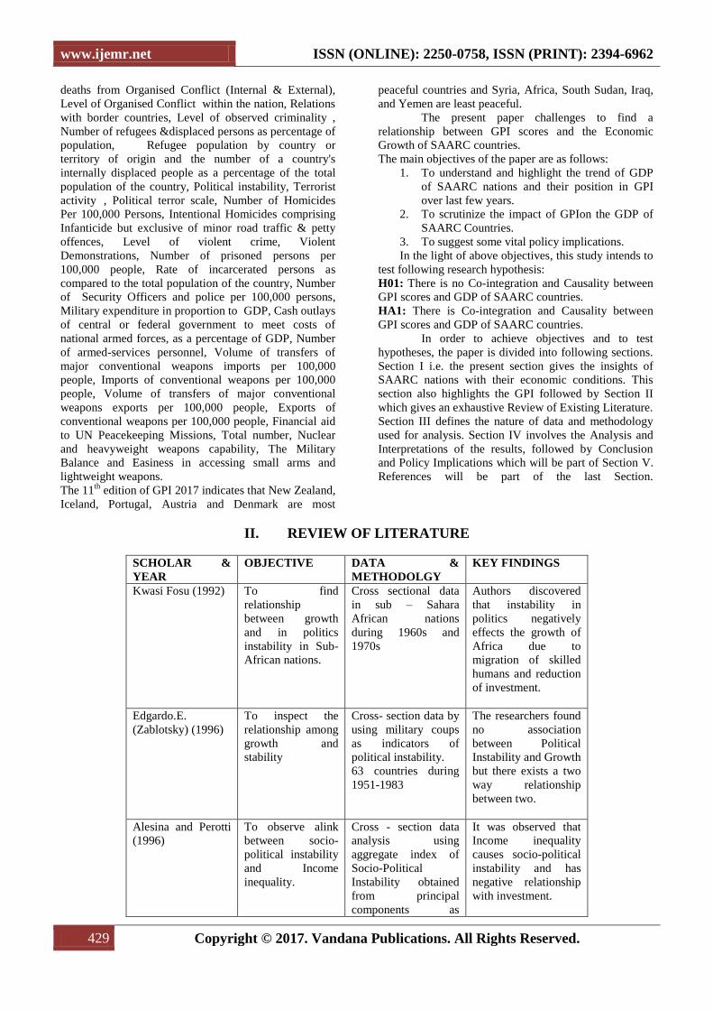
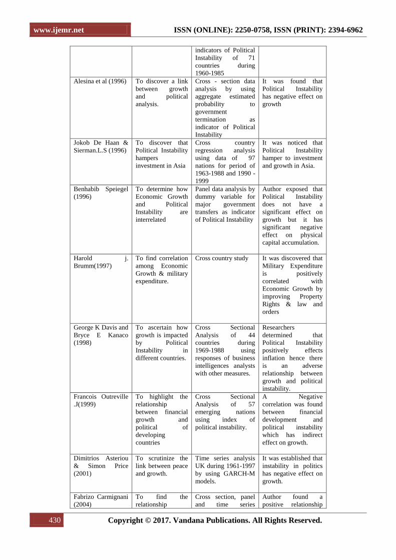
II. REVIEW OF LITERATURE
SCHOLAR &
YEAR
OBJECTIVE DATA &
METHODOLGY
KEY FINDINGS
Kwasi Fosu (1992) To find
relationship
between growth
and in politics
instability in Sub-
African nations.
Cross sectional data
in sub – Sahara
African nations
during 1960s and
1970s
Authors discovered
that instability in
politics negatively
effects the growth of
Africa due to
migration of skilled
humans and reduction
of investment.
Edgardo.E.
(Zablotsky) (1996)
To inspect the
relationship among
growth and
stability
Cross- section data by
using military coups
as indicators of
political instability.
63 countries during
1951-1983
The researchers found
no association
between Political
Instability and Growth
but there exists a two
way relationship
between two.
Alesina and Perotti
(1996)
To observe alink
between socio-
political instability
and Income
inequality.
Cross - section data
analysis using
aggregate index of
Socio-Political
Instability obtained
from principal
components as
It was observed that
Income inequality
causes socio-political
instability and has
negative relationship
with investment.
www.ijemr.net ISSN (ONLINE): 2250-0758, ISSN (PRINT): 2394-6962
430 Copyright © 2017. Vandana Publications. All Rights Reserved.
indicators of Political
Instability of 71
countries during
1960-1985
Alesina et al (1996) To discover a link
between growth
and political
analysis.
Cross - section data
analysis by using
aggregate estimated
probability to
government
termination as
indicator of Political
Instability
It was found that
Political Instability
has negative effect on
growth
Jokob De Haan &
Sierman.L.S (1996)
To discover that
Political Instability
hampers
investment in Asia
Cross country
regression analysis
using data of 97
nations for period of
1963-1988 and 1990 -
1999
It was noticed that
Political Instability
hamper to investment
and growth in Asia.
Benhabib Speiegel
(1996)
To determine how
Economic Growth
and Political
Instability are
interrelated
Panel data analysis by
dummy variable for
major government
transfers as indicator
of Political Instability
Author exposed that
Political Instability
does not have a
significant effect on
growth but it has
significant negative
effect on physical
capital accumulation.
Harold j.
Brumm(1997)
To find correlation
among Economic
Growth & military
expenditure.
Cross country study It was discovered that
Military Expenditure
is positively
correlated with
Economic Growth by
improving Property
Rights & law and
orders
George K Davis and
Bryce E Kanaco
(1998)
To ascertain how
growth is impacted
by Political
Instability in
different countries.
Cross Sectional
Analysis of 44
countries during
1969-1988 using
responses of business
intelligences analysts
with other measures.
Researchers
determined that
Political Instability
positively effects
inflation hence there
is an adverse
relationship between
growth and political
instability.
Francois Outreville
.J(1999)
To highlight the
relationship
between financial
growth and
political of
developing
countries
Cross Sectional
Analysis of 57
emerging nations
using index of
political instability.
A Negative
correlation was found
between financial
development and
political instability
which has indirect
effect on growth.
Dimitrios Asteriou
& Simon Price
(2001)
To scrutinize the
link between peace
and growth.
Time series analysis
UK during 1961-1997
by using GARCH-M
models.
It was established that
instability in politics
has negative effect on
growth.
Fabrizo Carmignani
(2004)
To find the
relationship
Cross section, panel
and time series
Author found a
positive relationship

www.ijemr.net ISSN (ONLINE): 2250-0758, ISSN (PRINT): 2394-6962
431 Copyright © 2017. Vandana Publications. All Rights Reserved.
between Political
Instability and
Growth, Fiscal
Policy and
Monetary Policy.
analysis with
summary of broad
literature
between all
parameters.
Selvarathinam
Santhirasegaram
(2008)
To investigate the
influence of Peace
on Economic
Growth in
emerging nations.
Pooled data Analysis
of 70 underdeveloped
nations from 2000-
2004 using OLS
Econometric
Methods.
Author emphasized
that peace as
determinant of growth
should be
incorporated within
growth theories in
future.
Deyshappriya(2015) To model the effect
of Corruption and
Peace on
Economic Growth.
Cross-country
analysis which
focuses of countries.
Corruption and Peace
were represented by
corruption perception
index and GPI.
OLS estimates was
applied to analyse the
data.
Result established that
Corruption adversely
affects the per capita
economic growth,
while peace stimulates
the economic growth.
Balami & et. al
(2016)
To inspect the
association
between peace,
security and
inclusive growth in
Nigeria.
Existing literature Result suggested that
Peace and Security
are very vital and
instrumental in the
Economic
development of any
nation.
III. DATA AND METHODOLOGY
The data have been collected from various
sources like, the handbook of statistics of Reserve Bank
of India, International Financial Statistics, and IMF and
from the GPI .The data for the study has been collected
from 2008 to 2017.
Owing to the nature of data, it becomes very
important to test whether data is stationary or not before
applying test like Cointegration, Granger Causality and
OLS technique as the data is time series. We use
different unit root tests, namely Augmented- Dicky
Fuller (ADF) to add robustness in the results. We first
study the data properties from an econometric
perspective starting with the Stationarity of Data. We
employ cointegration technique to understand the
causality in GPI and GDP of SAARC Countries. The
Stationarity of data has been tested using ADF test. The
ADF test uses the presence of Unit Root as the null
hypothesis. The next logical step for our purpose is to
study the Granger-causal relationship between the
variables.
The Time Series data has been analyzed
Country-wise as well as Panel Data Cross Sectional
Fixed Effect Analyses has been done.
IV. RESULTS AND ANALYSIS
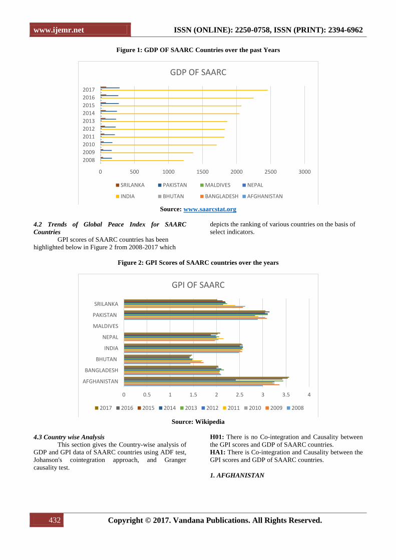
4.1 Trends and composition of GDP of SAARC
Countries
To understand the effect of GPI on GDP of
SAARC Countries, it is important to examine the trends
of GDP of SAARC Countries over the past years, which
will give an inclusive picture of how the landscape of
SAARC countries have changed over the years. Figure 1
given below gives the overview of trend of GDP of
SAARC Countries form 2008-2017.
www.ijemr.net ISSN (ONLINE): 2250-0758, ISSN (PRINT): 2394-6962
432 Copyright © 2017. Vandana Publications. All Rights Reserved.
Figure 1: GDP OF SAARC Countries over the past Years
Source: www.saarcstat.org
4.2 Trends of Global Peace Index for SAARC
Countries
GPI scores of SAARC countries has been
highlighted below in Figure 2 from 2008-2017 which
depicts the ranking of various countries on the basis of
select indicators.
Figure 2: GPI Scores of SAARC countries over the years
Source: Wikipedia
4.3 Country wise Analysis
This section gives the Country-wise analysis of
GDP and GPI data of SAARC countries using ADF test,
Johanson's cointegration approach, and Granger
causality test.
H01: There is no Co-integration and Causality between
the GPI scores and GDP of SAARC countries.
HA1: There is Co-integration and Causality between the
GPI scores and GDP of SAARC countries.
1. AFGHANISTAN
0 500 1000 1500 2000 2500 3000
2008
2009
2010
2011
2012
2013
2014
2015
2016
2017
GDP OF SAARC
SRILANKA PAKISTAN MALDIVES NEPAL
INDIA BHUTAN BANGLADESH AFGHANISTAN
0 0.5 1 1.5 2 2.5 3 3.5 4
AFGHANISTAN
BANGLADESH
BHUTAN
INDIA
NEPAL
MALDIVES
PAKISTAN
SRILANKA
GPI OF SAARC
2017 2016 2015 2014 2013 2012 2011 2010 2009 2008
www.ijemr.net ISSN (ONLINE): 2250-0758, ISSN (PRINT): 2394-6962
433 Copyright © 2017. Vandana Publications. All Rights Reserved.
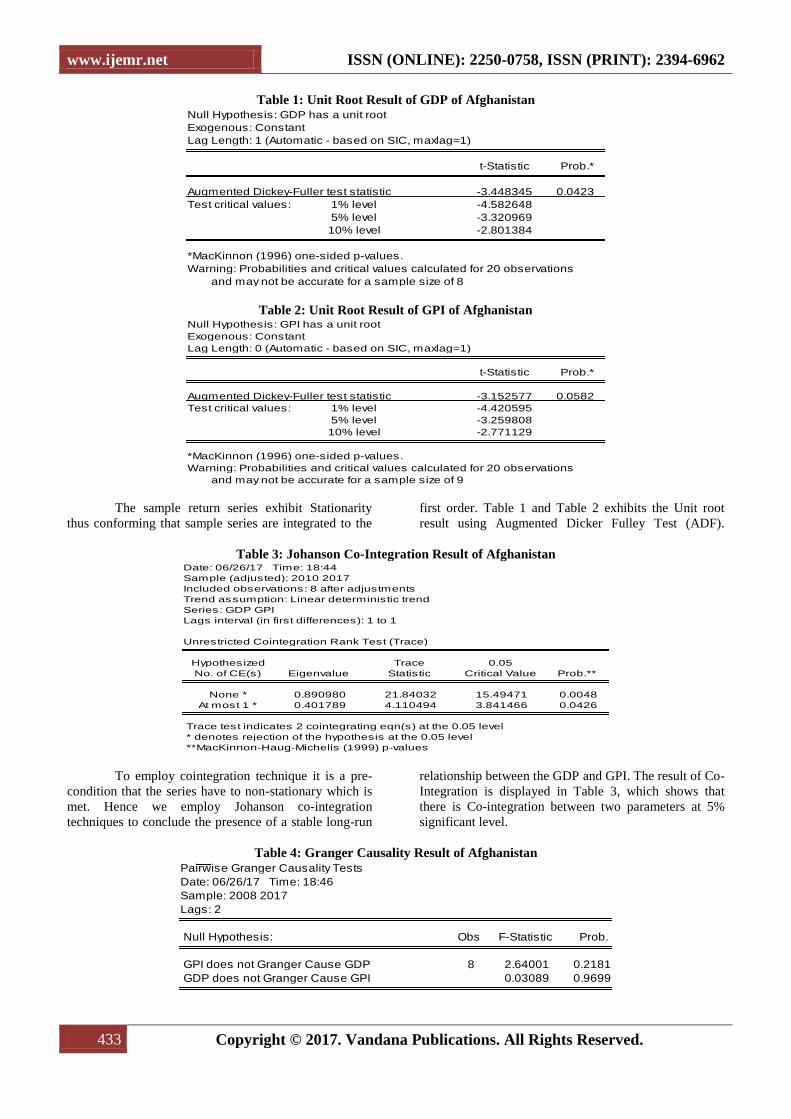
Table 1: Unit Root Result of GDP of Afghanistan
Table 2: Unit Root Result of GPI of Afghanistan
The sample return series exhibit Stationarity
thus conforming that sample series are integrated to the
first order. Table 1 and Table 2 exhibits the Unit root
result using Augmented Dicker Fulley Test (ADF).
Table 3: Johanson Co-Integration Result of Afghanistan
To employ cointegration technique it is a pre-
condition that the series have to non-stationary which is
met. Hence we employ Johanson co-integration
techniques to conclude the presence of a stable long-run
relationship between the GDP and GPI. The result of Co-
Integration is displayed in Table 3, which shows that
there is Co-integration between two parameters at 5%
significant level.
Table 4: Granger Causality Result of Afghanistan
Null Hypothesis: GDP has a unit root
Exogenous: Constant
Lag Length: 1 (Automatic - based on SIC, maxlag=1)
t-Statistic Prob.*
Augmented Dickey-Fuller test statistic -3.448345 0.0423
Test critical values: 1% level -4.582648
5% level -3.320969
10% level -2.801384
*MacKinnon (1996) one-sided p-values.
Warning: Probabilities and critical values calculated for 20 observations
and may not be accurate for a sample size of 8
Null Hypothesis: GPI has a unit root
Exogenous: Constant
Lag Length: 0 (Automatic - based on SIC, maxlag=1)
t-Statistic Prob.*
Augmented Dickey-Fuller test statistic -3.152577 0.0582
Test critical values: 1% level -4.420595
5% level -3.259808
10% level -2.771129
*MacKinnon (1996) one-sided p-values.
Warning: Probabilities and critical values calculated for 20 observations
and may not be accurate for a sample size of 9
Date: 06/26/17 Time: 18:44
Sample (adjusted): 2010 2017
Included observations: 8 after adjustments
Trend assumption: Linear deterministic trend
Series: GDP GPI
Lags interval (in first differences): 1 to 1
Unrestricted Cointegration Rank Test (Trace)
Hypothesized Trace 0.05
No. of CE(s) Eigenvalue Statistic Critical Value Prob.**
None * 0.890980 21.84032 15.49471 0.0048
At most 1 * 0.401789 4.110494 3.841466 0.0426
Trace test indicates 2 cointegrating eqn(s) at the 0.05 level
* denotes rejection of the hypothesis at the 0.05 level
**MacKinnon-Haug-Michelis (1999) p-values
Pairwise Granger Causality Tests
Date: 06/26/17 Time: 18:46
Sample: 2008 2017
Lags: 2
Null Hypothesis: Obs F-Statistic Prob.
GPI does not Granger Cause GDP 8 2.64001 0.2181
GDP does not Granger Cause GPI 0.03089 0.9699

www.ijemr.net ISSN (ONLINE): 2250-0758, ISSN (PRINT): 2394-6962
434 Copyright © 2017. Vandana Publications. All Rights Reserved.
After analysing that there is a significant cointegration in
the sample series, we employ Granger Causality Test to
test the Causality between the two variables and the
results are proven in Table 4 which verifies a uni variate
causality between the two variables.
2. BANGLADESH
Table 5: Unit Root Result of GDP of Bangladesh
Table 6: Unit Root Result of GPI of Bangladesh
Table 5 and Table 6 displays the stationarity on
2nd
level difference, hence, co-integration test can be
employed.
Table 7: Johanson Co-Integration Result of Bangladesh
Table 7 reveals the result of Co-Integration test
showing the co-integration between both the variables at
5% significant level at 1st difference.
Null Hypothesis: D(GDP,2) has a unit root
Exogenous: Constant
Lag Length: 1 (Automatic - based on SIC, maxlag=1)
t-Statistic Prob.*
Augmented Dickey-Fuller test statistic -3.043056 0.0844
Test critical values: 1% level -5.119808
5% level -3.519595
10% level -2.898418
*MacKinnon (1996) one-sided p-values.
Warning: Probabilities and critical values calculated for 20 observations
and may not be accurate for a sample size of 6
Null Hypothesis: GPI has a unit root
Exogenous: Constant
Lag Length: 0 (Automatic - based on SIC, maxlag=1)
t-Statistic Prob.*
Augmented Dickey-Fuller test statistic -2.053937 0.2630
Test critical values: 1% level -4.420595
5% level -3.259808
10% level -2.771129
*MacKinnon (1996) one-sided p-values.
Warning: Probabilities and critical values calculated for 20 observations
and may not be accurate for a sample size of 9
Date: 06/26/17 Time: 18:54
Sample (adjusted): 2010 2017
Included observations: 8 after adjustments
Trend assumption: Linear deterministic trend
Series: GDP GPI
Lags interval (in first differences): 1 to 1
Unrestricted Cointegration Rank Test (Trace)
Hypothesized Trace 0.05
No. of CE(s) Eigenvalue Statistic Critical Value Prob.**
None * 0.867584 18.55498 15.49471 0.0167
At most 1 0.257378 2.380542 3.841466 0.1229
Trace test indicates 1 cointegrating eqn(s) at the 0.05 level
* denotes rejection of the hypothesis at the 0.05 level
**MacKinnon-Haug-Michelis (1999) p-values
www.ijemr.net ISSN (ONLINE): 2250-0758, ISSN (PRINT): 2394-6962
435 Copyright © 2017. Vandana Publications. All Rights Reserved.
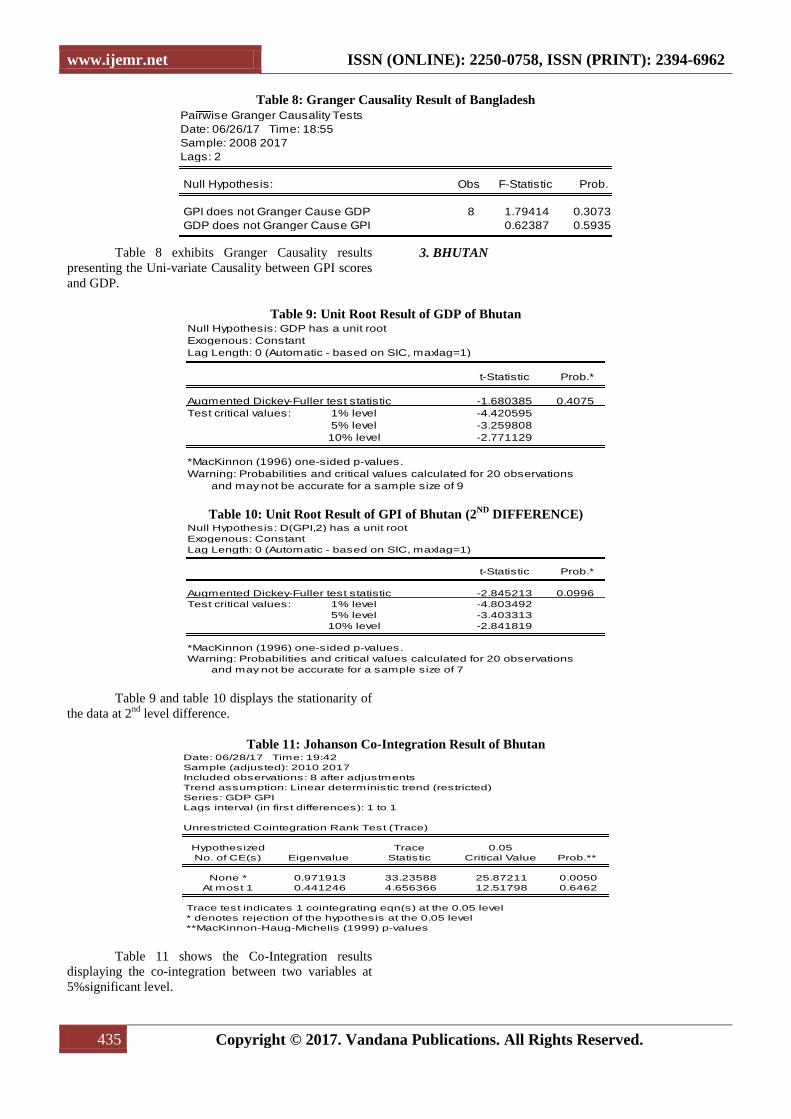
Table 8: Granger Causality Result of Bangladesh
Table 8 exhibits Granger Causality results
presenting the Uni-variate Causality between GPI scores
and GDP.
3. BHUTAN
Table 9: Unit Root Result of GDP of Bhutan
Table 10: Unit Root Result of GPI of Bhutan (2ND
DIFFERENCE)
Table 9 and table 10 displays the stationarity of
the data at 2nd
level difference.
Table 11: Johanson Co-Integration Result of Bhutan
Table 11 shows the Co-Integration results
displaying the co-integration between two variables at
5%significant level.
Pairwise Granger Causality Tests
Date: 06/26/17 Time: 18:55
Sample: 2008 2017
Lags: 2
Null Hypothesis: Obs F-Statistic Prob.
GPI does not Granger Cause GDP 8 1.79414 0.3073
GDP does not Granger Cause GPI 0.62387 0.5935
Null Hypothesis: GDP has a unit root
Exogenous: Constant
Lag Length: 0 (Automatic - based on SIC, maxlag=1)
t-Statistic Prob.*
Augmented Dickey-Fuller test statistic -1.680385 0.4075
Test critical values: 1% level -4.420595
5% level -3.259808
10% level -2.771129
*MacKinnon (1996) one-sided p-values.
Warning: Probabilities and critical values calculated for 20 observations
and may not be accurate for a sample size of 9
Null Hypothesis: D(GPI,2) has a unit root
Exogenous: Constant
Lag Length: 0 (Automatic - based on SIC, maxlag=1)
t-Statistic Prob.*
Augmented Dickey-Fuller test statistic -2.845213 0.0996
Test critical values: 1% level -4.803492
5% level -3.403313
10% level -2.841819
*MacKinnon (1996) one-sided p-values.
Warning: Probabilities and critical values calculated for 20 observations
and may not be accurate for a sample size of 7
Date: 06/28/17 Time: 19:42
Sample (adjusted): 2010 2017
Included observations: 8 after adjustments
Trend assumption: Linear deterministic trend (restricted)
Series: GDP GPI
Lags interval (in first differences): 1 to 1
Unrestricted Cointegration Rank Test (Trace)
Hypothesized Trace 0.05
No. of CE(s) Eigenvalue Statistic Critical Value Prob.**
None * 0.971913 33.23588 25.87211 0.0050
At most 1 0.441246 4.656366 12.51798 0.6462
Trace test indicates 1 cointegrating eqn(s) at the 0.05 level
* denotes rejection of the hypothesis at the 0.05 level
**MacKinnon-Haug-Michelis (1999) p-values

www.ijemr.net ISSN (ONLINE): 2250-0758, ISSN (PRINT): 2394-6962
436 Copyright © 2017. Vandana Publications. All Rights Reserved.
Table 12: Granger Causality Result of Bhutan
Table 12 exhibits that there is non-existence of
Causality between two variables, hence unveils a
negative relationship between the two variables.
4. INDIA
Table 13: Unit Root Result of GDP of India
Table 14: Unit Root Result of GPI of India
Table 13 and Table 14 confirms that the data is
stationary as p value is less than 0.05.
Table 15: Johanson Co-Integration Result of India
Table 15 unveils the Co-integration between
GPI scores and GDP at 5 percent significant level.
Pairwise Granger Causality Tests
Date: 06/28/17 Time: 19:43
Sample: 2008 2017
Lags: 2
Null Hypothesis: Obs F-Statistic Prob.
GPI does not Granger Cause GDP 8 0.83009 0.5165
GDP does not Granger Cause GPI 0.29620 0.7631
Null Hypothesis: GDP has a unit root
Exogenous: Constant
Lag Length: 0 (Automatic - based on SIC, maxlag=1)
t-Statistic Prob.*
Augmented Dickey-Fuller test statistic -4.932776 0.0052
Test critical values: 1% level -4.420595
5% level -3.259808
10% level -2.771129
*MacKinnon (1996) one-sided p-values.
Warning: Probabilities and critical values calculated for 20 observations
and may not be accurate for a sample size of 9
Null Hypothesis: D(GPI) has a unit root
Exogenous: Constant
Lag Length: 0 (Automatic - based on SIC, maxlag=1)
t-Statistic Prob.*
Augmented Dickey-Fuller test statistic -2.312888 0.1894
Test critical values: 1% level -4.582648
5% level -3.320969
10% level -2.801384
*MacKinnon (1996) one-sided p-values.
Warning: Probabilities and critical values calculated for 20 observations
and may not be accurate for a sample size of 8
Date: 06/28/17 Time: 19:46
Sample (adjusted): 2010 2017
Included observations: 8 after adjustments
Trend assumption: Linear deterministic trend (restricted)
Series: GDP GPI
Lags interval (in first differences): 1 to 1
Unrestricted Cointegration Rank Test (Trace)
Hypothesized Trace 0.05
No. of CE(s) Eigenvalue Statistic Critical Value Prob.**
None * 0.999826 77.46435 25.87211 0.0000
At most 1 0.641295 8.202040 12.51798 0.2356
Trace test indicates 1 cointegrating eqn(s) at the 0.05 level
* denotes rejection of the hypothesis at the 0.05 level
**MacKinnon-Haug-Michelis (1999) p-values

www.ijemr.net ISSN (ONLINE): 2250-0758, ISSN (PRINT): 2394-6962
437 Copyright © 2017. Vandana Publications. All Rights Reserved.
Table 16: Granger Causality Result of India
Table 16 discloses Uni- variate causality
between GDP and GPI scores of India. 5. NEPAL
Table 17: Unit Root Result of GDP of Nepal
Table 18: Unit Root Result of GPI of Nepal
Table 17 and table 18 approves the stationarity of data as
p value is less than 0.05, henceforth, Co-integration test
can be performed.
Table 19: Johanson Cointegration Result of Nepal
Table 19 supports the cointegration between
GPI scores and GDPat 5 % significant level.
Pairwise Granger Causality Tests
Date: 06/28/17 Time: 19:47
Sample: 2008 2017
Lags: 2
Null Hypothesis: Obs F-Statistic Prob.
GPI does not Granger Cause GDP 8 0.16840 0.8525
GDP does not Granger Cause GPI 1.31740 0.3885
Null Hypothesis: D(GDP) has a unit root
Exogenous: Constant
Lag Length: 0 (Automatic - based on SIC, maxlag=1)
t-Statistic Prob.*
Augmented Dickey-Fuller test statistic -15.49320 0.0000
Test critical values: 1% level -4.582648
5% level -3.320969
10% level -2.801384
*MacKinnon (1996) one-sided p-values.
Warning: Probabilities and critical values calculated for 20 observations
and may not be accurate for a sample size of 8
Null Hypothesis: D(GPI) has a unit root
Exogenous: Constant
Lag Length: 0 (Automatic - based on SIC, maxlag=1)
t-Statistic Prob.*
Augmented Dickey-Fuller test statistic -2.508265 0.1472
Test critical values: 1% level -4.582648
5% level -3.320969
10% level -2.801384
*MacKinnon (1996) one-sided p-values.
Warning: Probabilities and critical values calculated for 20 observations
and may not be accurate for a sample size of 8
Date: 06/28/17 Time: 19:17
Sample (adjusted): 2010 2017
Included observations: 8 after adjustments
Trend assumption: Linear deterministic trend (restricted)
Series: GDP GPI
Lags interval (in first differences): 1 to 1
Unrestricted Cointegration Rank Test (Trace)
Hypothesized Trace 0.05
No. of CE(s) Eigenvalue Statistic Critical Value Prob.**
None * 0.944145 30.19275 25.87211 0.0136
At most 1 0.588973 7.112764 12.51798 0.3329
Trace test indicates 1 cointegrating eqn(s) at the 0.05 level
* denotes rejection of the hypothesis at the 0.05 level
**MacKinnon-Haug-Michelis (1999) p-values

www.ijemr.net ISSN (ONLINE): 2250-0758, ISSN (PRINT): 2394-6962
438 Copyright © 2017. Vandana Publications. All Rights Reserved.
Table 20: Granger Causality Result of Nepal
Table 20 exhibits the results of Granger
Causality test which confirms non-existence of causality
in GDP and GPI of Nepal, hence, approves anadverse
relationship between the two variables.
6. PAKISTAN
Table 21: Unit Root Result of GDP of Pakistan
Table 22: Unit Root Result of GPI of Pakistan
Table 21 and table 22 displays the result of Unit root
confirming that the data is stationary.
Table 23: Johanson Co-Integration Result of Pakistan
Table 23 exhibits that there exists co-integration between
the two variables at 5% significant level.
Pairwise Granger Causality Tests
Date: 06/28/17 Time: 19:19
Sample: 2008 2017
Lags: 2
Null Hypothesis: Obs F-Statistic Prob.
GPI does not Granger Cause GDP 8 0.31260 0.7528
GDP does not Granger Cause GPI 0.00736 0.9927
Null Hypothesis: GDP has a unit root
Exogenous: Constant
Lag Length: 0 (Automatic - based on SIC, maxlag=1)
t-Statistic Prob.*
Augmented Dickey-Fuller test statistic -2.554155 0.1354
Test critical values: 1% level -4.420595
5% level -3.259808
10% level -2.771129
*MacKinnon (1996) one-sided p-values.
Warning: Probabilities and critical values calculated for 20 observations
and may not be accurate for a sample size of 9
Null Hypothesis: D(GPI) has a unit root
Exogenous: Constant
Lag Length: 1 (Automatic - based on SIC, maxlag=1)
t-Statistic Prob.*
Augmented Dickey-Fuller test statistic -4.470954 0.0144
Test critical values: 1% level -4.803492
5% level -3.403313
10% level -2.841819
*MacKinnon (1996) one-sided p-values.
Warning: Probabilities and critical values calculated for 20 observations
and may not be accurate for a sample size of 7
Date: 06/28/17 Time: 19:27
Sample (adjusted): 2010 2017
Included observations: 8 after adjustments
Trend assumption: No deterministic trend (restricted constant)
Series: GDP GPI
Lags interval (in first differences): 1 to 1
Unrestricted Cointegration Rank Test (Trace)
Hypothesized Trace 0.05
No. of CE(s) Eigenvalue Statistic Critical Value Prob.**
None * 0.764753 21.91404 20.26184 0.0294
At most 1 * 0.725316 10.33707 9.164546 0.0298
Trace test indicates 2 cointegrating eqn(s) at the 0.05 level
* denotes rejection of the hypothesis at the 0.05 level
**MacKinnon-Haug-Michelis (1999) p-values

www.ijemr.net ISSN (ONLINE): 2250-0758, ISSN (PRINT): 2394-6962
439 Copyright © 2017. Vandana Publications. All Rights Reserved.
Table 24: Granger Causality Result of Pakistan
Table 24 reveals the result of granger causality test,
confirming a Bi-variate causality, hence, showing a
positive relationship between GDP and GPI of Pakistan.
7. SRILANKA
Table 25: Unit Root Result of GDP of Srilanka
Table 26: Unit Root Result of GPI of Srilanka
Table 25 and Table 26 shows the result of Unit
root depicting that the data is stationary and co-
integration test can be performed on data.
Table 27: Johanson Co-Integration Result of Srilanka
Table 27 gives the result of co-integration
showing co-integration between two variables at 5%
significant level.
Pairwise Granger Causality Tests
Date: 06/28/17 Time: 19:28
Sample: 2008 2017
Lags: 2
Null Hypothesis: Obs F-Statistic Prob.
GPI does not Granger Cause GDP 8 1.72682 0.3169
GDP does not Granger Cause GPI 0.88632 0.4984
Null Hypothesis: GDP has a unit root
Exogenous: Constant
Lag Length: 1 (Automatic - based on SIC, maxlag=1)
t-Statistic Prob.*
Augmented Dickey-Fuller test statistic -2.591386 0.1322
Test critical values: 1% level -4.582648
5% level -3.320969
10% level -2.801384
*MacKinnon (1996) one-sided p-values.
Warning: Probabilities and critical values calculated for 20 observations
and may not be accurate for a sample size of 8
Null Hypothesis: D(GPI) has a unit root
Exogenous: Constant
Lag Length: 0 (Automatic - based on SIC, maxlag=1)
t-Statistic Prob.*
Augmented Dickey-Fuller test statistic -1.762658 0.3693
Test critical values: 1% level -4.582648
5% level -3.320969
10% level -2.801384
*MacKinnon (1996) one-sided p-values.
Warning: Probabilities and critical values calculated for 20 observations
and may not be accurate for a sample size of 8
Date: 06/28/17 Time: 19:32
Sample (adjusted): 2010 2017
Included observations: 8 after adjustments
Trend assumption: Linear deterministic trend
Series: GDP GPI
Lags interval (in first differences): 1 to 1
Unrestricted Cointegration Rank Test (Trace)
Hypothesized Trace 0.05
No. of CE(s) Eigenvalue Statistic Critical Value Prob.**
None * 0.822732 22.61000 15.49471 0.0036
At most 1 * 0.665848 8.769266 3.841466 0.0031
Trace test indicates 2 cointegrating eqn(s) at the 0.05 level
* denotes rejection of the hypothesis at the 0.05 level
**MacKinnon-Haug-Michelis (1999) p-values

www.ijemr.net ISSN (ONLINE): 2250-0758, ISSN (PRINT): 2394-6962
440 Copyright © 2017. Vandana Publications. All Rights Reserved.
Table 28: Granger Causality Result of Srilanka
Table 28 depicts the result of Granger Causality test
confirming a Uni-variate causality between the two
variables.
4.4 PANEL DATA CROSS SECTIONAL ANALYSIS
USING FIXED EFFECT
Table 29: Unit Root Result of GDP of SAARC Countries
Table 30: Unit Root Result of GPI of SAARC Countries
Pairwise Granger Causality Tests
Date: 06/28/17 Time: 19:33
Sample: 2008 2017
Lags: 2
Null Hypothesis: Obs F-Statistic Prob.
GPI does not Granger Cause GDP 8 0.77684 0.5347
GDP does not Granger Cause GPI 1.70778 0.3198
Null Hypothesis: GDP has a unit root
Exogenous: Constant
Lag Length: 0 (Automatic - based on SIC, maxlag=11)
t-Statistic Prob.*
Augmented Dickey-Fuller test statistic -2.307853 0.1721
Test critical values: 1% level -3.515536
5% level -2.898623
10% level -2.586605
*MacKinnon (1996) one-sided p-values.
Augmented Dickey-Fuller Test Equation
Dependent Variable: D(GDP)
Method: Least Squares
Date: 06/19/17 Time: 19:10
Sample (adjusted): 2 80
Included observations: 79 after adjustments
Variable Coefficient Std. Error t-Statistic Prob.
GDP(-1) -0.128810 0.055814 -2.307853 0.0237
C 36.67603 37.97292 0.965847 0.3371
R-squared 0.064696 Mean dependent var 0.978481
Adjusted R-squared 0.052549 S.D. dependent var 316.6735
S.E. of regression 308.2407 Akaike info criterion 14.32463
Sum squared resid 7315949. Schwarz criterion 14.38462
Log likelihood -563.8229 Hannan-Quinn criter. 14.34866
F-statistic 5.326186 Durbin-Watson stat 1.927156
Prob(F-statistic) 0.023694
Null Hypothesis: GPI has a unit root
Exogenous: Constant
Lag Length: 0 (Automatic - based on SIC, maxlag=11)
t-Statistic Prob.*
Augmented Dickey-Fuller test statistic -3.610749 0.0076
Test critical values: 1% level -3.515536
5% level -2.898623
10% level -2.586605
*MacKinnon (1996) one-sided p-values.
Augmented Dickey-Fuller Test Equation
Dependent Variable: D(GPI)
Method: Least Squares
Date: 06/19/17 Time: 19:10
Sample (adjusted): 2 80
Included observations: 79 after adjustments
Variable Coefficient Std. Error t-Statistic Prob.
GPI(-1) -0.283699 0.078571 -3.610749 0.0005
C 0.564945 0.178715 3.161147 0.0022
R-squared 0.144801 Mean dependent var -0.012418
Adjusted R-squared 0.133694 S.D. dependent var 0.762208
S.E. of regression 0.709429 Akaike info criterion 2.176277
Sum squared resid 38.75327 Schwarz criterion 2.236263
Log likelihood -83.96295 Hannan-Quinn criter. 2.200310
F-statistic 13.03751 Durbin-Watson stat 2.249462
Prob(F-statistic) 0.000541
www.ijemr.net ISSN (ONLINE): 2250-0758, ISSN (PRINT): 2394-6962
441 Copyright © 2017. Vandana Publications. All Rights Reserved.
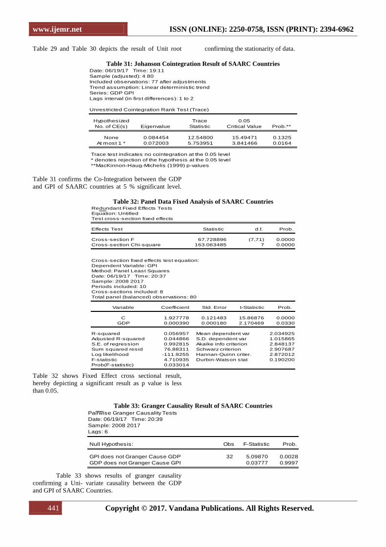
Table 29 and Table 30 depicts the result of Unit root confirming the stationarity of data.
Table 31: Johanson Cointegration Result of SAARC Countries
Table 31 confirms the Co-Integration between the GDP
and GPI of SAARC countries at 5 % significant level.
Table 32: Panel Data Fixed Analysis of SAARC Countries
Table 32 shows Fixed Effect cross sectional result,
hereby depicting a significant result as p value is less
than 0.05.
Table 33: Granger Causality Result of SAARC Countries
Table 33 shows results of granger causality
confirming a Uni- variate causality between the GDP
and GPI of SAARC Countries.
Date: 06/19/17 Time: 19:11
Sample (adjusted): 4 80
Included observations: 77 after adjustments
Trend assumption: Linear deterministic trend
Series: GDP GPI
Lags interval (in first differences): 1 to 2
Unrestricted Cointegration Rank Test (Trace)
Hypothesized Trace 0.05
No. of CE(s) Eigenvalue Statistic Critical Value Prob.**
None 0.084454 12.54800 15.49471 0.1325
At most 1 * 0.072003 5.753951 3.841466 0.0164
Trace test indicates no cointegration at the 0.05 level
* denotes rejection of the hypothesis at the 0.05 level
**MacKinnon-Haug-Michelis (1999) p-values
Redundant Fixed Effects Tests
Equation: Untitled
Test cross-section fixed effects
Effects Test Statistic d.f. Prob.
Cross-section F 67.728896 (7,71) 0.0000
Cross-section Chi-square 163.063485 7 0.0000
Cross-section fixed effects test equation:
Dependent Variable: GPI
Method: Panel Least Squares
Date: 06/19/17 Time: 20:37
Sample: 2008 2017
Periods included: 10
Cross-sections included: 8
Total panel (balanced) observations: 80
Variable Coefficient Std. Error t-Statistic Prob.
C 1.927778 0.121483 15.86876 0.0000
GDP 0.000390 0.000180 2.170469 0.0330
R-squared 0.056957 Mean dependent var 2.034925
Adjusted R-squared 0.044866 S.D. dependent var 1.015865
S.E. of regression 0.992815 Akaike info criterion 2.848137
Sum squared resid 76.88311 Schwarz criterion 2.907687
Log likelihood -111.9255 Hannan-Quinn criter. 2.872012
F-statistic 4.710935 Durbin-Watson stat 0.190200
Prob(F-statistic) 0.033014
Pairwise Granger Causality Tests
Date: 06/19/17 Time: 20:39
Sample: 2008 2017
Lags: 6
Null Hypothesis: Obs F-Statistic Prob.
GPI does not Granger Cause GDP 32 5.09870 0.0028
GDP does not Granger Cause GPI 0.03777 0.9997
www.ijemr.net ISSN (ONLINE): 2250-0758, ISSN (PRINT): 2394-6962
442 Copyright © 2017. Vandana Publications. All Rights Reserved.
V. CONCLUSION AND
IMPLICATIONS
The main purpose of the study is to comprehend
the effect of peace on the growth of SAARC countries.
Out of 8 member nations of SAARC countries, Maldives
is not been part of GPI, hence, our study excludes the
Maldives from the analyses. The result of OLS and
pooled cross- sectional analyses proposes that in
Afghanistan, Bangladesh, India and Srilanka, a Uni-
Variate causality between GPI scores and GDP, hence,
rejecting the null hypotheses, whereas, in Pakistan there
is a Bi-Variate causality between the two variables
depicting that peace and economic growth both of
Pakistan are inter-related. On the other hand, result for
Nepal and Bhutan depicts a negative relationship
between two variables, hence, accepting the null
Hypotheses. The results would help the nations to
develop the strategies to maintain peace and harmony
resulting in the growth and development.
REFRENCES
[1] Alesina and Alberto. (1996). Political instability and
Economic Growth. Journal of Economic Growth. Vol,
1/2, pp. 189-211.
[2] Alesina and Perotti. (1996). Income distribution,
political instability and investment. European economic
review, Vol 46, pp.1203-23.
[3] Balami &et. al. (2016). The Imperative of Peace and
Security forthe Attainment of Inclusive Growth in
Nigeria, European Journal of Research in Social
Sciences, Vol. 4 No. 2, ISSN 2056-5429.
[4] Benhabib, Jess and Rustichini, Aldo. (1996).Social
Conflict and Growth. Journal of Economic Growth. Vol,
1, issue, 1, pp. 127-42.
[5] Campos and Jeffrey B. Nugent. (2003).
Consequences of social and political instability.
Economica, 70, pp.533-49.
[6] Chetan Ghate, Quan Vu Le and Paul J. Zak. (2003).
Optimum fiscal policy in an economy facing socio-
political instability. Review of economic development,
7, 4, pp.583-98.
[7] David Fielding. (2003). Modelling Political
Instability and Economic Performance: Israeli
Investment during the Intifada, Economica 70, pp. 159 –
86.
[8] Deyshappriya. (2015). Do corruption and peace
affect economic growth? Evidences from the cross-
country analysis. Journal of Social and Economic
Development, Volume 17, Issue 2, pp 135–147. DOI:
10.1007/s40847-015-0016-1
[9] Dimitrios Asteriou, Simon Price. (2001). Political
Instability and Economic Growth: UK Time Series
Evidence, Scottish Journal of Political Economy, 48, 4,
pp. 383-399.
[10] Edgardo E. Zablotsky. (1996). Political stability and
economic growth –Two way relation, working paper
No.103, Centre for macroeconomic studies, Argentina.
[11] Fabrizo Carmignani. (2004). Efficiency of
institutions, political stability and economic dynamics.
Working paper, United Nation Economic Commission
for Europe (UNECE).
[12] Francois Outreville .J. (1999). Financial
development, and human capital and political stability,
UNCTAD discussion paper, No 142, available at
www.unctad.org/en/pub/public
[13] George K Davis and Bryce E Kanaco. (1998).
Inflation, inflation uncertainty, political stability, and
economic growth. Working paper, department of
economics, Miani University, Oxford Ohio, 45056.
[14] Harold j. Brumm. (1997) .Military Spending,
Government Disarray, and Economic Growth: A Cross-
Country Empirical Analysis Journal of Macroeconomics,
19, 4, pp. 827–838.
[15] James L.Butkiewicz and Halit Yanikkaya. (2005).
the impact of socio-political instability on economic
growth: Analysis and implications, Journal of policy
modelling, Vol 27, pp.629-45.
[16] Jokob de Haan and Clemens.L.J Sierman. (1996).
Political instability, freedom, and economic growth:
Some further evidence, Economic Development and
Cultural Change, Vol, 44 (2).
[17] John Gerring, PhilipBond, William T.B and Carola
Mereno. (2005). Democracy and economic growth: A
historical perspectives, World Politics, a quarterly
journal of international relation, 57/4. And full version
available in Web Site in May 2007 at
http://web.bu.edu/pardee/events/conferences/2007/
[17] Kwasi Fosu. (1992). Political instability and
economic growth, economic development and cultural
change, Vol, 40, pp. 829-41.
[18] Ludovic Comeau.Jr. (2003). Democracy and
growth: A relationship revised. Eastern economic
journal, 29, pp.1-19.
[19] Richard Jing – A- Pin. (2006). on the measurement
of political stability and its impacts on growth, Working
paper, department of economics, university of
Groningen, Nether Land.
[20] Selvarathinam Santhirasegaram. (2008). Peace and
Economic Growth in Developing Countries: Pooled Data
Cross -Country Empirical Study. International
Conference on Applied Economics – ICOAE 2008.
[21] Suleiman Abu-Bader, Aamer S. Abu-Qarn. (2003).
Government expenditures, military spending and
economic growth: causality evidence from Egypt, Israel,
and Syria, Journal of Policy Modelling, 25, pp. 567–583
World development index (WDI) of World Bank group,
Data query, Available in June 2007 at
http://genderstats.worldbank.org/dataquery/