Relational development site appraisal model for the ...

Relational development site appraisal model for the deployment of Marine Energy

Convertors in Scotland

Mark H, Wemyss

Submitted for the degree of Doctor of Philosophy

Heriot-Watt University

International Centre for Island Technology (ICIT), Institute of Petroleum Engineering

May/2014

The copyright in this thesis is owned by the author. Any quotation from the thesis or

use of any of the information contained in it must acknowledge this thesis as the source

of the quotation or information.

ABSTRACT

The use of GIS tools in marine spatial planning has become widespread. Such tools

however often prescribe sterilized zones from a developer’s perspective (e.g. protected

areas) and use surrogate indicators of wave and tidal resource with these being used to

suggest areas of likely commercial development.

The work undertaken in this thesis follows a more dynamic approach which has

developed software to model the development appraisal process for wave and tidal

projects. This means the most economically feasible sites for development can be

located, taking into account factors (such as cable costs) ignored where resolve

parameters alone are used in marine spatial planning.

Moreover the model developed enables contrasting scenarios for differing harvesting

technologies, grid connection points, cable types, port facilities to be examined and for

specific improvement plans for such infrastructure to be investigated.

i

ACKNOWLEDGEMENTS

All staff and students at the International Centre of Island Technology (ICIT) and in

particular both supervisors: Professor Jon Side and Dr Sandy Kerr.

Dr Mike Bell, Internal Examiner, Heriot Watt University.

Dr Keith Tovey, External Examiner, University of East Anglia.

Lesley Johnston, Ken, Kathleen and Struan Wemyss. For their dedicated support.

ii

DECLARATION STATEMENT

iii

TABLE OF CONTENTS

CHAPTER 1 – INTRODUCTION Page 1

1.1 Overall project aim

1.2 Research methodology

1.3 Renewable energy policy Page 2

1.4 Marine Spatial Planning Page 7

1.4.1 MSP background and history Page 8

1.5 Previous similar work undertaken within Marine Spatial Planning,

marine renewable planning and other related research

Page 10

1.5.1 Strategic Environmental Assessment (SEA), by Scottish

Executive

1.5.2 Department of Trade and Industry (DTI) UK marine

renewable energy atlas

Page 11

1.5.3 The Department for Environment and Rural Affairs (Defra)

Irish Sea pilot

Page 12

1.5.4 Shetland Marine Spatial planning project Page 13

1.5.5 Other related work

1.6 Weaknesses with the Marine Spatial Planning and previous approaches Page 15

1.7 Dynamic Marine Spatial Planning tool Page 16

1.8 Research rationale and overarching challenge Page 18

1.9 Research objectives and aims Page 19

1.10 Likely end users and their requirements

1.11 Structure of thesis

Page 20

CHAPTER 2 – STUDY AREA BACKGROUND AND BOUNDARIES Page 21

2.1 The study area

2.1.1 Other physical characteristics and resource Page 23

2.1.2 Electrical grid Page 24

2.1.3 Ports Page 29

2.2 Marine Energy Devices (MECs) Page 30

2.2.1 Technological review Page 31

2.2.2 Wave energy and devices Page 32

2.2.3 Wave devices coastal (fixed) methods Page 34

iv

2.2.4 Wave devices offshore methods Page 35

2.2.5 Tidal energy and technology Page 36

2.2.6 Tidal barrage technology Page 36

2.2.7 Tidal lagoon technology Page 38

2.2.8 Tidal current technology Page 39

2.2.9 Description of relevant devices used in modelling Page 40

CHAPTER 3 – DATA REQUIREMENTS AND MODEL DESIGN Page 44

3.1 External datasets

3.2 Self constructed datasets Page 46

3.3 Automated model datasets Page 47

3.4 Top level design for the model with the identified datasets, and project

aims

Page 48

3.5 Overall description of the program model design Page 50

3.5.1 Finding a valid site

3.5.2 Determine a cable, costs and revenue Page 54

3.5.3 Determine installation, decommissioning and financial costs Page 57

3.5.4 Conclusion drawn from top level design Page 58

3.6 Design analysis for working example of model Page 59

3.7 Datasets selected to construct model 1

3.7.1 Acquired external data

3.7.2 Self constructed datasets review Page 63

3.7 3 Automated model data

3.8 Manipulation of available datasets Page 64

3.8.1 GEBCO data

3.8.2 DTI data Page 66

3.8.3 Self constructed and automated data Page 70

3.8 4 Random access file format Page 72

3.9 Working model design Page 73

3.9.1 Low level design of model construction Page 75

3.9.2 Low level design of supporting applications and test modules

3.10 Dataset design and methodology for testing Page 77

3.10.1 White and black box testing Page 78

3.10.2 In built test facility random access files Page 79

3.10.3 Twin application operation Page 80

v

3.10.4 Other datasets and datasets produced due to the program

design

Page 80

3.10.5 VRML (Virtual Reality Modelling Language) data handling

3.10.6 Other tools such a Google Earth

Page 82

CHAPTER 4 – OPERATION OF MODEL Page 83

4.1 Twin modes of operation

4.2 Graphical User Interface (GUI) Page 84

4.2.1 Visual Basic (VB) as a Graphical User Interface (GUI) programming

solution

Page 85

4.2.2 Event driven and structured programming methods

4.3 Batch operation and outputs Page 86

4.4 User operation and outputs Page 88

4.5 The function of the application model

4.5.1 User operation example walk through Page 89

4.5.2 Batch operation example walk through

Page 106

CHAPTER 5 MODEL TESTING RESULTS Page 118

5.1 Structure and methodology of model result testing

5.2 Batch results from first run Page 120

5.3 Batch results after change to resource test logic (second run) Page 124

5.4 Batch results after changes, and additions to various database

parameters (third run)

Page 125

5.5 Batch results after alteration to cables record set (fourth and fifth runs) Page 129

5.5.1 Batch results, fourth run

5.5.2 Batch results, fifth run Page 133

5.5.3 Batch results, comparison between fourth and fifth runs Page 137

5.6 Overall summary of batch test runs Page 140

5.7 Test comparison of batch and user facilities

Page 141

CHAPTER 6 ILLUSTRATED EXAMPLE Page 144

6.1 Data to be added to include the proposed grid upgrade

6.2 Model run before and after proposed grid upgrade added to database Page 147

6.3 Model results and comparison of before and after model results Page 148

6.4 Further changes to input data with resulting site outputs Page 149

vi

6.5 Economic distribution Page 152

6.6 Overall findings

Page 154

CHAPTER 7–HOW THE MODEL COULD BE IMPROVED Page 156

7.1 Missing constraints and functionality

7.2 Data and program resolution Page 159

7.3 Further functionality

7.3.1 Logical detail Page 160

7.3.2 Data addition

7.3.3 Result data management Page 161

7.3.4 Human Computer Interaction (HCI) considerations

7.3.5 Economic features Page 162

7.3.6 Cable modelling

7.3.7 Pipeline and shore station model Page 163

7.3.8 Hydrodynamic model Page 164

7.3.9 Automated automisation

7.3.10 Automated data formatting Page 165

7.4 Feedback and possible further usage

CHAPTER 8–DISCUSSION AND CONCLUSION

Page 167

REFERENCES Page 172

APPENDIX A BATCH ALGORITHMS AND CALCULATIONS

THE MODEL USES

Page 185

A.1 Determining a spatial distribution for each device determined by water

depth

A.2 Determining a spatial distribution for each device determined by

resource

A.3 Determining a spatial distribution for each device determined by

distance to land

Page 186

A.4 Determining an overall spatial distribution for each device determined

by water depth, resource, and distance to land

A.5 Constructing a distance matrix from each site to closest power station Page 187

A.6 Constructing a distance matrix from each site to closest port Page 188

vii

A.7 Calculate cable costs for each site against valid location for each

device

Page 189

A.8 Calculate the number of devices required and device output at a given

site

A.9 Calculate the device cost for a given valid site Page 193

A.10 Add device costs to cable costs Page 194

A.11 Calculate revenue at each site for each valid device

A.12 Calculate installation depth factor for each site

A.13 Calculate installation distance factor for each site Page 195

A.14 Calculate overall installation and decommissioning Costs

A.15 Add installation costs to device and cable costs Page 196

A.16 Determine profit/loss for each valid device at each valid site

A.17 Calculate distance between two given points

A.18 Record dataset range values Page 198

A.19 Output dataset range values

A.20 Clear output dataset range

A.21 Write valid results dataset Page 199

A.22 Clear valid results dataset

A.23 Calculate cable cost without device validation

APPENDIX B ALGORITHMS AND CALCULATIONS REQUIRED

FOR MODEL USER OPERATION

Page 201

B.1 Find GEBCO depth

B.2 Find DTI resolution data Page 202

B.3 Find closest landing point Page 203

B.4 Find closest port Page 204

B.5 Calculate distance between two given points Page 205

B.6 Select a device

B.7 Display union device results Page 208

B.8 Calculate site output Page 209

B.9 Calculate cable details

B.10 Calculate overall device cost Page 211

B.11 Calculate installation depth factor

B.12 Calculate installation distance factor

B.13 Calculate user installation costs Page 212

viii

B.14 Calculate decommissioning cost

B.15 Calculate revenue Page 213

B.16 Calculate total profit/loss

APPENDIX C GLOBAL ALGORITHMS AND CALCULATIONS

REQUIRED FOR GLOBAL OPERATIONS

Page 214

C.1 Set global variables

C.2 Calculate device parameters

C.3 Calculate power station and port minutes Page 215

APPENDIX D ALGORITHMS AND CALCULATIONS REQUIRED

FOR RANDOM ACCESS TEST FACILITY

Page 216

D.1 Setup display combo for test function

D.2 Random access file test facility display

D.3 Calculate random access data file statistics Page 217

APPENDIX E ALGORITHMS AND CALCULATIONS USED FOR

DISPLAY RESULTS FACILITY

Page 219

E.1 Display overall profit/loss statistics

E.2 Load files with valid results Page 220

E.3 Display results Page 221

E.4 Sort results

APPENDIX F OTHER WINDOWS RELATED METHODS AND

FUNCTIONS

Page 223

F.1 Enter location of deployment site screen, Form_Load

F.2 Enter location of deployment site screen, location combo box events

F.3 Enter location of deployment site screen, enter location, command

button

Page 225

F.4 Characteristics of site screen “Find device”, command button Page 226

F.5 Device results screen, select device, command button Page 227

F.6 Batch menu, run batch, command button

F.7 Load entity record set data

ix

APPENDIX G, LIST OF DATASETS USED BY THE MODEL (AS

BUILT)

Page 229

G.1 DTI Datasets, in form: Name of dataset (unit)

G.2 GEBCO Data

G.3 Automated static model data Page 230

G.4 Automated model data, for any given device

G.5 Microsoft Access Data Tables Page 232

APPENDIX H Page 233

H.1 Batch results from first run

H.1.1 Device 5 (Pelamis)

H.1.2 Device 75 (Test wave device) Page 239

H.1.3 Device 76 (Test tidal device) Page 246

H.2 Batch results, second run Page 251

H.2.1 Device 5 (Pelamis) results Page 252

H.2.2 Device 75 (Test wave device) results

H.2.3 Device 76 (Test tidal device) results Page 255

H.3 Batch results, third run

H.3.1 Device 5 (Pelamis) Page 256

H.3.2 Device 7 (OSPREY)

H.3.3 Device 13 (Wave Star) Page 257

H.3.4 Device 45 (Marine current turbines) Page 260

H.3.5 Device 47 (TidE1)

H.3.6 Device 56 (Hammerfest Strøm) Page 261

H.3.7 Device 75 (Test wave device) Page 262

H.3.8 Device 76 (Test tidal device) Page 266

APPENDIX I, LIST OF DEVICES MODEL USES Page 267

I.1 Wave Devices

I.2 Tidal Devices Page 268

I.3 Devices identified, but not processed by model due to insufficient data,

in form: name of device, company/developer.

Page 269

APPENDIX J, PSEUDO CODE OF MODEL (AS BUILT)

FUNCTIONS, BATCH OPERATION

Page 271

x

J.1 Determining a spatial distribution for each device determined by water

depth

J.2 Determining a spatial distribution for each device determined by

resource

Page 272

J.3 Determining a spatial distribution for each device determined by

distance to land

Page 273

J.4 Determining an overall spatial distribution for each device determined

by water depth, resource, and distance to land

J.5 Constructing a distance matrix from each site to closest power station Page 274

J.6 Construct a distance matrix from each site to closest port Page 275

J.7 Calculate cable costs for each site against valid location for each device Page 276

J.8 Calculate the number of devices required and device output at a given

site

Page 278

J.9 Calculate the device cost for a given valid site Page 279

J.10 Add device costs to cable costs Page 280

J.11 Calculate revenue at each site for each valid device Page 282

J.12 Calculate installation depth factor for each site Page 283

J.13 Calculate installation distance factor for each site Page 284

J.14 Calculate overall installation costs

J.15 Add installation costs to device and cable costs Page 286

J.16 Determine profit/loss for each valid device at each valid site Page 287

J.17 Calculate Distance Page 288

APPENDIX K, GUIDE TO ACCOMPANYING ELECTRONIC

MATERIAL

Page 290

K.1 Software used and compatibility

K.2 Submitted electronic program files

K.3 Program data

K.4 Installing and using software application Page 291

xi

LIST OF TABLES AND FIGURES

Figure 1.1 Showing a view of the simplified approaches taken by a

traditional MSP method and Dynamic Marine Spatial

Planning tool developed in this research. The MSP

approach gathers data which is mapped and used for

zoning, while the method in this research tests the

available data at each site for each form of technology

(variables that can all be changed) to produce dynamic

results.

Page 18

Figure 2.1 Maximum geographical boundary of the project. Page 21

Figure 2.2 Showing the DTI data coverage around Scotland. The

extent of the tidal data is shown in purple. The wave

resource resolution grid can be seen further to the west.

Page 22

Figure 2.3 Showing the range for offshore distances within the study

area. This image has been captured using the DTI data,

(BERR, 2008).

Page 23

Figure 2.4 Showing the annual mean tidal power (kW/m2) for the

study area on the left, and the annual mean wave power

on the right (kW/m). These images have been captured

using the DTI data (BERR, 2008).

Page 24

Figure 2.5 Pentland Firth and Orkney waters round 1 development

sites. Source Crown Estate.

Page 27

Figure 2.6 Showing a summary of devices that feature in the data

modelling and analysis later in the thesis. These

parameters within the database are key to the

calculations of the model. Values that are unknown

(Null) will not allow the model to consider the devices

beyond the initial stages of testing. The reason these

devices do feature in the more detailed modelling is

because these values are updated in the model testing in

Chapter 5 of the thesis.

Page 43

Figure 3.1 Showing a top level design for what is required to satisfy

the aims of the model. Most of the processes have been

Page 49

xii

simplified (grouped into higher level single processes) for

this level of design. The blue arrows represent the site

analysis aspect of the design, while the green ones

represent economic aspects.

Figure 3.2 Showing an expanded view of the likely physical

constraints (and therefore datasets) that the device is

tested against at every site.

Page 51

Figure 3.3 Showing an expanded view of the non physical

constraints (and therefore datasets) that the device is

tested against at every site.

Page 52

Figure 3.4 Showing an expanded view of the more detailed site

analysis incorporating a hydrodynamic modelling

element.

Page 54

Figure 3.5 Showing an expanded view of how the cable, various

costs and revenue are determined.

Page 56

Figure 3.6 Showing an expanded view of how the installation,

decommissioning, project costs, and profit/loss are

determined.

Page 58

Figure 3.7 Top level design of overall ideal model, with dash

sections showing what was omitted from the example

model top level design.

Page 60

Figure 3.8 Showing the boundary of the truncated GEBCO dataset. Page 65

Figure 3.9 Showing an example of the boundaries and data

resolution changes for the DTI datasets.

Page 68

Figure 3.10 Showing the annual mean tidal power density, more

importantly it shows the boundaries where the main tidal

values exist, i.e. areas not in grey.

Page 69

Figure 3.11 Example model, top level design. Hierarchical data flow

chart of the batch operation’s main methods. More

emphasis is given in this design to the data flows between

the main processes.

Page 74

Figure 3.12 Showing a VRML image of the GEBCO Bathymetry data

viewed from an elevated viewpoint to essentially show a

2D representation of the study area. Data in VRML can

be viewed in 3D in graphical viewer i.e. effectively the

Page 81

xiii

data at any point can be navigated to by the user. The

above image is in a looking down view of the dataset to

represent a map with a flat layer added at sea level.

Figure 3.13 Showing a VRML image of the GEBCO Bathymetry data

from an elevated viewpoint rotated on the x axis to show

the 3D element of the data, i.e. white above sea level is

land, and seabed below. West of Ireland the data shows a

greater distance between the flat sea level blue layer, and

the bottom white layer, which represents the descending

water depth from the continental shelf.

Page 82

Figure 4.1 Showing the initial progress bar and Enter location of

deployment site screen which is displayed when the

application data are fully loaded. For the batch menu the

user does not need to select a location which is only for

the user operation. A proceeding menu could have been

used for Batch and User, however this would have

created an unnecessary level and screen at this stage.

Page 89

Figure 4.2 characteristics of site screen in the user operation.. Page 90

Figure 4.3 Showing the difference between the two distance

calculation methods. Positions C to D is the point to

point method where the exact positions are measured.

Positions A to B is the centre file locations dictated by the

resolution of the data.

Page 92

Figure 4.4 Showing a plot in Google Earth of the UK, Ireland and

Isle of Man coastal power station and grid landing points

that are stored in the model database.

Page 93

Figure 4.5 Power station/landing point details screen Page 96

Figure 4.6 Port details screen Page 97

Figure 4.7 Device results screen Page 98

Figure 4.8 Marine energy device screen Page 100

Figure 4.9 Marine energy company details screen Page 102

Figure 4.10 Cable and costing results screen Page 103

Figure 4.11 Cable and costing results screen after alteration of

number of devices.

Page 104

Figure 4.12 Cable details screen. Note there are some fields that do Page 105

xiv

not contain data as these are not used in the working

model and were to be part of the full model.

Figure 4.13 Batch menu screen Page 106

Figure 4.14 Testing facility screen loaded from selecting “Data Test”

at 4.13. The form shows the results of position Row 1

Column 0 (start position) of the Mean water depth from

tidal file. The “Char Size” indicates the number of

characters in each data cell within the Random Access

File, giving the total variable length.

Page 107

Figure 4.15 Testing facility screen showing an alternative test

example, this time showing a valid result that is

connected to the Pelamis wave device ID 5. The Device

ID has been entered into the “Select File” text box to

select the file which is described below.

Page 108

Figure 4.16 A file directory view showing the sub directory structure

where the various output files are located.

Page 110

Figure 4.17 A file directory view showing the various individual

output files from within the profit loss result directory.

Note all files are the same size which is due to the

random access format.

Page 111

Figure 4.18 Run individual batch processes screen Page 113

Figure 4.19 Profit/loss results/display screen Page 114

Figure 4.20 Profit/loss results screen with another example, Device

76, Test tidal device

Page 116

Figure 4.21 Profit/loss results screen with an example to show “All”

valid results for all valid devices. The display shows the

full path name which was required during the

development, but a refinement would be to simplify the

path with a filter that could be turned on or off. A full

discussion of the various improvements that can be made

in the future is discussed within Chapter 7.

Page 117

Figure 5.1 Showing each model test result run undertaken with the

relationship between the model runs and data

comparisons. The initial first run was found to have a

problem with the model logic. Run 2 therefore cures this

Page 119

xv

and the results are compared to confirm this. Runs 2 and

3 are also compared to determine user level changes

made to input datasets. Various valid site inconsistencies

were found in the results of run 3, so run 4 and 5 were

undertaken to replicate run 2 and 3 after the required

modifications were undertaken to the model data.

Therefore the results comparison between runs 4 and 5

directly replicated the analysis undertaken between 2 and

3. The results comparison between runs 2 and 4, & 3 and

5 were to confirm the various required alterations to the

model were successful and that the latest tests were

giving acceptable results. Within each run the valid

devices for a site were reviewed.

Figure 5.2 Showing the valid devices found at valid sites for each

particular run.

Page 120

Figure 5.3 Showing the DTI peak flow for a mean spring tide (left)

and the annual mean tidal power density (right) with

corresponding keys. The narrow inner channels to the

north of the isles (which is Yell sound and Bluemull

sound) show a light blue colour for the peak flow which is

hard to identify on the key scale. The power density map

shows the value as 0.00. Therefore, it can be confirmed

from the atlas and a study of the underlying data values,

the actual resource has not been identified.

Page 122

Figure 5.4 Showing the tidal resource data (each point being a site

with data from the DTI) which clearly shows missing data

from various coastal areas and inner sounds.

Page 123

Figure 5.5 Showing a later version of the DTI data which has gone

through various upgrades and improvements since the

initial release which is used in this research. It can be

seen that the data still does not include any resource

indication for the Shetland channels in question.

Figure 5.6 Showing the difference between the first and second batch

runs in terms of number of sites per device and cable.

The results show the difference after the logic for the

Page 124

xvi

resource test was modified not to include a conflicting

resource at sites.

Figure 5.7 Showing the distribution change for all devices before

(first run) and after (second run) the alteration to the

code. Device 5 plotted in blue, Device 75 in black, and

Device 76 in red. Note there is only one red plot in the

second run, in the Solway Firth at the very bottom of the

map. All devices show a distinct reduction.

Page 125

Figure 5.8 Showing the difference between the second and third

batch run with the various planned changes.

Page 127


(second run) and after (third run) the alteration to

various controlling data sources. Although at this scale it

is difficult to notice the change in detail, it can be seen

various new sites have been found, which is of course the

new devices now making it to a profit/loss result. Device

5 plotted in Blue, Device 75 in Black, Device 76 in Red,

Device 56 in Yellow, Device 47 in Pink, Device 7 in Grey,

and Device 13 in Brown.

Page 128

Figure 5.10 Showing the relationship between the data in the second

and fourth run.

Page 130


(second run) and after (fourth run) the alteration to

various controlling data sources. At this scale it is

extremely difficult to identify any difference in the two

sets. Device 5 plotted in Blue, Device 75 in Black, Device

76 in Red.

Figure 5.12 Showing an overall distribution of Device 75 for the

second (left) and fourth runs. The colour scheme follow

the logics that the more intense the colour (red) the more

cost effective the site, i.e. higher the profit/loss result. At

this resolution it is very difficult to identify the difference

in device numbers.

Page 132

Figure 5.13 The left image shows the data difference between the

second and fourth runs for Device 75. Each point

Page 133

xvii

indicates an individual site. 495 sites were identified

which are all within 33kV and 132kV distance voids from

various landing points. This problem was corrected in

the fourth run and therefore these sites were identified as

a result. To the right is an example for Shetland which

has been focused to a level where valid (and void) sites

can be distinguished from a valid site dataset previous to

the cable data alteration.

Figure 5.14 Showing the relationship between the data in the third

and fifth run.

Page 134


(third run) and after (fifth run) the alteration to various

controlling data sources. At this scale it is very difficult

to identify any difference in the two sets. Device 5 plotted

in Blue, Device 75 in Black, Device 76 in Red, Device 56

in Yellow, Device 47 in Pink, Device 7 in Grey, and

Device 13 in Brown.

Page 135

Figure 5.16 Showing an overall distribution of Device 75 for the third

(left) and fifth runs. At this resolution it is very difficult to

identify the difference in device numbers, or the

distribution change of the sites per cost.

Page 136

Figure 5.17 Showing the data difference between the fifth and third

runs for Device 75. Each point indicates an individual

site. 581 sites were identified which are all within 33kV

and 132kV distance voids from various landing points.

This problem was corrected for the fourth run, and

therefore these sites were identified as a result.

Page 137

Figure 5.18 Showing the relationship between the data in the fourth

and fifth run for device 75, Test wave device.

Page 138


(fourth run) and after (fifth run) the alteration to various

controlling data sources. At this scale it is difficult to

identify the changes clearly, however the additional

devices and sites can be seen on close inspection. Device

5 plotted in Blue, Device 75 in Black, Device 76 in Red,

xviii

Device 56 in Yellow, Device 47 in Pink, Device 7 in Grey,

and Device 13 in Brown.


fourth (left) and fifth runs. The distribution change of the

sites per cost can be identified with careful inspection. In

the current analysis for Device 75 the number and

location of sites were identical for both runs. The only

changes appeared in the cost values in the financial

model.

Page 139

Figure 5.21 Showing the final profit/loss result screen for the user

method at site 57.96 (57° 57’ 0”) north -7.09 (7° 5’ 0”)

west (or in data location terms data row 213, data

column 100). To get to this point the user selected 200

(which is the minimum number of devices for the HVDC

cable type at this distance from landing point) Test wave

devices, which is Device 75 within the database.

Page 142

Figure 5.22 Showing a data test enquiry for the same location (57.96°

north, 7.09° west / data row 213 data column 100) for the

Test wave device (Device 75) for the minimum profit/loss

result for a HVDC cable, i.e. the data inputs as for the

user example above.

Figure 6.1 Showing one of the scenarios the Crown Estate has

proposed for offshore grid development.

Page 145

Figure 6.2 Showing the offshore points added to the landing

point/connection dataset.

Page 146

Figure 6.3 Showing the plotted offshore connection points.

Figure 6.4 Showing the relationship between the data in the sixth

and seventh runs. There is only 1 new sites identified.

Page 148

Figure 6.5 Showing the relationship between the data in the eighth

and ninth runs

Page 149

Figure 6.6 Showing the valid results for run 8 (left in turquoise only)

with entire results for run 9 (additional new sites shown

in red). On the right are the newly found sites for run 9

only. Note the new connection points plotted in yellow.

Page 150

Figure 6.7 Showing the specific new sites found for Device 4 and

xix

Device 5 in relation to the connection points added.

Device 4 in pink, Device 5 in blue, with connection points

in yellow. Note no new sites were found in relation to the

sites added around the Firth of Forth/Tayside.

Figure 6.8 Showing the valid sites for the 3 tidal devices, Devices 46,

56, and 64, which are all in the same area of the Pentland

Firth. This distribution did not alter after the addition of

the new offshore connection points. Note that in 4 of the

above locations more than one device was found at the

same site.

Page 152


fourth (left) and fifth runs. Note the lack of sites found in

the south east for this hypothetical device set with

favourable parameter data.

Page 153

Figure 6.10 Showing the 2 sites in Shetland (blue) that experienced a

lower profit loss result as a result of the new connection

points which are shown in yellow and black. The other

yellow plot is the offshore connection point added in run

5 that allowed a significant reduction in cost with the

hypothetical device which had a favourable water depth

and distance to land set to allow offshore sites to be

found.

Figure A.1 Showing a matrix of a search area of valid (green) and

red (invalid) sites. If the originating site is 1 (that cannot

fulfil the output required for a valid cable type) the

search would test adjacent sites such as 2, 3, 4, 5, 6, 7

and 8. If these additional sites still did not produce the

desired output, further sites could be tested, although it is

likely some boundary rules would exist. In the example

above only sites directly connected spatially are

considered to be valid (green) i.e. the connected sites can

make up one continuous arrangement.

Page 193

Figure H.1 Device 5 (Pelamis wave device) showing the 3rd

4th

and

5th

ranked 33kV sites on the west coast of the Orkney

Isles.

Page 233

xx

Figure H.2 Device 5 (Pelamis wave device) showing the 1st and

6th

ranked 33kV sites in the Passage of Tiree between the

islands of Mull and Coll/Tiree.

Page 234

Figure H.3 Device 5 (Pelamis wave device) showing the 2nd

ranked

33kV site in St Magnus Bay on the west coast of the

Shetland Mainland.

Figure H.4 Characteristics of site screen showing the site details of

the 6th

most likely development sites between the islands

of Mull and Coll and Tiree.

Page 235

Figure H.5 Site Details of the 4th

site, off Westray, Orkney. Page 237


, 3rd

and

4th

ranked 132kV sites around Unst and Sumburgh.

Shetland, like many of the remote areas that follow, only

has a 33kV network so it is broadly assumed such a

development could only take place with further

developments to the onshore grid. The model for these

tests is set so that onshore capacity is available to

highlight the potential offshore sites.

Figure H.7 Device 5 (Pelamis wave device) showing the 1st, 5th and

6th

ranked 132kV sites off the west coast of Lewis, and

Westray, Orkney. The distance (calculated in Google

Earth) for the most feasible site in Orkney to the closest

grid connection point is EMEC tidal site (plotted in blue)

at 33.36 km.

Page 238

Figure H.8 Device 5 (Pelamis wave device) showing 1st and 2

nd (all)

ranked HVDC sites off Cape Wrath. The blue plot shown

in this instance is to the closest grid connection point,

Dounreay Power Station in Caithness 66.78 km.

Page 239

Figure H.9 Device 75 (Test wave device) showing the 5th

, 6th

, and

8th

ranked 33kV sites around the Isle of Tiree.

Page 240

Figure H.10 Device 75 (Test wave device) showing the1st to 4th

, 7 th

,

9th

and 10th

ranked 33kV sites around Eday in the Orkney

Isles.

Figure H.11 showing the Orkney Islands with each point representing

where a DTI water depth value exists. The scale values

Page 241

xxi

have been inverted so that lighter shades represent the

higher values, this is to help highlight the shoreline

regions that is the area of concern. It is also worth

noting the various resource datasets are the same

resolution, which will not show up the true potential of

the tidal channels around Orkney.

Figure H.12 Device 75 (Test wave device) showing the 1st, 3

rd, 6

th and

9th

ranked 132kV sites around the Shetland Isles.

Page 242

Figure H.13 Device 75 (Test wave device) showing the 2nd

, 4th, and

7th

ranked 132kV sites around North Ronaldsay, Orkney.

While the current development allows for different cable

types, other current or future constraints such as the

current regional grid network (currently, 33kV in

Orkney) should be addressed in future developments.

Figure H.14 Device 75 (Test wave device) showing the 5th, 8th, and

10th

ranked 132kV sites off the west coast of Lewis.

Page 243

Figure H.15 Device 75 (Test wave device) showing the, 3rd

, 4th

, 6th

, 7th

,

8th

, 9th

, and 10th

ranked HVDC sites off the West coast of

the Isle of Harris. The landing point for such a

development in this case is over 50km away at Loch

Carnan in South Uist.

Figure H.16 Device 75 (Test wave device) showing the1st, 2

nd and 5

th

ranked HVDC sites off the west coast of the Isle of Lewis.

Note the other development sites off the Isle of Harris

shown in Figure H.15, are the sites at the southern end of

this plot. These have been included to show the

relationship between the two sites.

Page 244


to the

31985th

ranked (i.e. 8 most unlikely) HVDC sites which

are located in the North Sea. The furthest most point

from significant land (which does not include Fair Isle)

being 99.35 km.

Page 245


and the

31983rd

ranked HVDC sites which are located west of the

Shetland Isles. The furthest most point from land being

xxii

81.46 km. Note within the DTI data an island such as

Foula/Fair Isle are not considered to be a significant

land mass and therefore the distance calculation was

taken to the Shetland Mainland.

Figure H.19 Entire cable and site results for Device 75 (Test wave

device) showing the overall distribution. It is interesting

to note that with the favourable device data, the return of

sites was significant, however, there are still large areas

where the device did not return any valid sites, such as

the Minch, Moray Firth, the south east, and south west

perimeters of the study area. This is due to these areas

having a wave resource too low for the Test wave device

which is set at 27 kW/m.

6

Figure H.20 Device 76 (Test tidal device) with a 33kV cable, with the

1st to the 10

th ranked 33kV sites, which are located within

Hoy/Burra Sound, and the Falls of Warness in Orkney.

Page 247

Figure H.21 Device 76 (Test tidal device) showing the 9th

and 10th

ranked 132kV sites which are located around Sanda Isle,

off the Mull of Kintyre.

Page 248

Figure H.22 Device 76 (Test tidal device) showing the 8th ranked

132kV site which is located in the Sound of Harris

between the isles of Harris and Berneray/North Uist.

Figure H.23 Device 76 (Test tidal device) showing the 1st to 5

th ranked

132kV sites which are located around North Ronaldsay in

the north of the Orkney Isles. Note the 4th

plot has ended

up on land according to the Google Map background

layer used for illustration purposes, which indicates a

problem with the DTI bathymetry data at this location.

Page 249

Figure H.24 Device 76 (Test tidal device) with a 132kV cable, with the

6th

and 7th

most likely development sites which are

located off Sumburgh Head, in the south of the Shetland

mainland.

Page 250

Figure H.25 Device 76 (Test tidal device) showing the 1st, 2

nd and 3

rd

ranked HVDC sites which are located in the Little Minch

of the North coast of the Isle of Skye.

xxiii

Figure H.26 Device 76 (Test tidal device), showing the 4th

to 10th

ranked HVDC sites which are located off the Mull of

Galloway.

1

Figure H.27 showing a GIS (MapInfo) plot for all sites found for

Device 76 Test tidal device.


nd, 3

rd, 5

th,

6th

, and 9th

ranked 33kV sites in the Passage of Tiree, and

8th

off Barra.

Page 252


, 7th

and 10th

ranked 33kV sites in the Orkney Isles.

Page 253


rd, 4

th,

6th

,7th

and 9th

ranked 132 kV sites off the west coast of

the Isle of Lewis.


, 5th

and 10th

ranked 132kV sites around the Shetland Isles.

Page 254

Figure H.32 Device 75 (Test wave device) showing the 1st to 10

th

ranked HVDC sites off the west coast of Harris and

Lewis.

Figure H.33 Device 76 (Test tidal device) showing the only site to

have passed to the final profit/loss results, which is off

Annan in the upper reaches of the Solway Firth.

Page 255

Figure H.34 Device 7 (OSPREY) showing the 1st to 4

th (all) ranked

33kV sites in the Orkney and Shetland Isles.

Page 256

Figure H.35 Device 7 (OSPREY) showing the 1st and 2

nd (all) ranked

132kV sites off the Isle of Skye and Mull respectively.

Page 257

Figure H.36 Device 13 (Wave Star) showing the 1st to 10

th ranked

33kV sites off the east coast off the Isle of Lewis,

Dounreay, and around the Orkney Isles.

Figure H.37 Device 13 (Wave Star) showing the 1st, 2

nd, 3

rd and 6th

ranked 132kV sites off the island of Yell, Unst and Fetlar

in the Shetland Isles.

Page 258

Figure H.38 Device 13 (Wave Star) showing the 5th

and 7th

ranked

132kV sites off the Buchan coast in the north east of

Scotland.


, 8th

, 9th

, and 10th

Page 259

xxiv

ranked 132kV sites off the west coast off the Isle of Lewis.


th ranked

HVDC sites in various locations around the western coast

and isles.

Figure H.41 Device 13 (Wave Star) showing the entire 253 results

plotted with the GIS package MapInfo.

0

Figure H.42 Device 47 (TidE1) showing the 1st (only) ranked 132kV

site off the Northern Irish coast.

Page 261

Figure H.43 Device 56 (Hammerfest Strøm) showing the 4th

to 7th

ranked 132kV sites off the north coast of the Isle of Man.

Figure H.44 Device 56 (Hammerfest Strøm) showing the 1st to 3

rd

ranked 132kV site off the Northern Irish coast.

Page 262

Figure H.45 Showing an overall distribution of device 75 for the

second (left) and third runs. At this resolution it is very

difficult to spot the difference in device numbers, however

the distribution change of the sites per cost can be

identified with careful inspection which is the result of the

newly added connection points (shown in blue) on the

east coast.

Page 263

Figure H.46 showing the new landing points at the centre of defined

study areas in the Pentland Firth (left yellow) and North

Sea (right blue).

Page 264

Figure H.47 showing the data difference between the second and third

runs (left), and third and second runs (right). Each point

indicates an individual site. 95 sites were identified in the

second run which were not found in the third run, and 9

sites were identified in the third run which were not in the

second run. These results point to a potential error in the

coding/data used.

Page 265

Figure K.1 Showing the structure of the C:\Mark Wemyss PhD Hand

in.

Page 292

Figure K.2 Showing the structure of the “C:\Mark Wemyss PhD

Hand in\Computer modelling\Visual Basic Version”.

Page 293

xxv

GLOSSARY

= - Equal

<> - Not equal

≥ - Greater than or equal

≤ - Less than or equal

3rd

Generation programming language - Computer environment that allows the

development of block structured programming.

4th

Generation programming language - Computer environment that allows the

development of event driving programming and graphical user interfaces.

33kv - 33 kilovolts, a standardised High Voltage rating.

132kv - 132 kilovolts, a standardised High Voltage rating.

AND gate - A logical operation that behaves according a truth table where a true output

is only gained when both inputs are true.

ANM - Active Network Management scheme.

ArcGIS - Geographical Information System (GIS) software package.

Batch processing - a series of commands/scripts/programs that are run from start to

finish without intervention.

BERR - Business Enterprise and Regulatory Reform.

Binary - A representation for numbers using only two digits 0 and 1.

Bitmap - Raster memory organisation of a file format used to store digital images.

BODC - British Oceanographic Data Centre.

Boolean - binary truth values of 0 or 1.

BWEA - British Wind Energy Association

CD ROM - Compact Disc Read Only Memory.

Combo (combination) box - Windows Graphical User Interface (GUI) facility to allow

predefined user input (data) to be selected from a list at run time. Also referred to as

drop down menu.

Command button - Windows Graphical User Interface (GUI) facility to allow code

(such as to open a new Form Window) to be executed from a specific place, i.e. a

button.

dBase - Database software package which was one of the first widely used Database

Management System (DBMS) for Microcomputers.

DCF - Discounted Cash Flow.

DECC - Department of Energy and Climate Change.

xxvi

Defra - Department for Environment, Food and Rural Affairs.

Drop down menu - Windows Graphical User Interface (GUI) facility to allow

predefined user input (data) to be selected from a list at run time. Also referred to as

Combo box (Combination box).

DTI - Department of Trade and Industry.

DVD - Digital Versatile Disc, an optical disc storage format.

EDF - Electricite de France.

EEZ - Exclusive Economic Zone.

ENSG - Electricity Networks Strategy Group.

EMEC - European Marine Energy Centre.

Excel - A Microsoft product allowing mathematical analysis of data via a variety of

tools and spreadsheets.

Event Driven Programming (EPD) language - A computing feature that allows

computer code to be controlled by user events, i.e. a window based language to allow

the development of windows applications/graphical user interfaces. EPD can also be

defined as a 4th

Generation Programming Language.

Form - Windows Graphical User Interface screen which will in most cases contain

many other Graphical User Interface items.

For loop - A function within a programming language that allows code to be repeated

for a given length of time.

GEBCO - General Bathymetric Chart of the Oceans

GIS - Graphical Information System, designed to capture, store, manipulate, analyze,

manage, and present all types of geographically referenced data.

Google Earth - Open sourced GIS based system.

Google Maps - Open source mapping system that can be integrated with Google Earth

to allow a front end display for GIS data.

GUI - Graphical User Interface.

GW - gigawatt, equal to one billion (109) watts or one thousand (10

3) megawatts.

High level programming language - Programming environments where English

syntax is used rather than binary or hexadecimal code. Languages of 3rd

generation

onwards.

Human Computer Interaction (HCI) - A term used for the study of the usability of

computers and computer software.

HVDC (High Voltage DC) - a High Voltage category that uses Direct Current

technology.

xxvii

ICIT - International Centre for Island Technology, Heriot-Watt University.

IDRISI - Geographical Information System (GIS) software.

IRR - Internal Rate of Return

km - Kilometre, equal to one thousand (103) metres.

kW/m kW/m2 - kilowatt per metre and kilowatt per metre squared , common units of

measurement for wave and tidal energy resource.

kV - kilovolt, equal to one thousand (103) volts.

kW - kilowatt, equal to one thousand (103) watts.

Kriging - An interpolation technique for obtaining estimates of unknown value from a

set of neighbouring control point values.

Latitude (Lat) - A system of referencing relative north-south locations on the earth's

surface. It is measured in degrees (°), minutes (‘), and seconds(’’) north or south of the

equator, incrementing to the poles.

List box - Windows Graphical User Interface (GUI) facility to allow list data to be

displayed.

LNR - Local Nature Reserves.

Longitude (Long) - A system of referencing relative east-west locations on the earth's

surface. It is measured in degrees (°), minutes (‘), and seconds (’’) east or west of the

Prime Meridian which runs through Greenwich, England.

Macro - A method in Microsoft office terms to allow multiple commands to be

executed.

MNR - Marine Nature Reserves.

Matrix - A rectangular arrangement of rows and columns containing data entries or

matrix elements.

MapInfo - Geographical Information System (GIS) software.

MEC - Marine Energy Convertor, generic term for both wave and tidal devices.

Megawatt - The megawatt is equal to one million (106) watts, or one thousand (10

3)

kilowatts.

Megawatt hour (MWh) - unit of energy equal to the work of one megawatt acting for

one hour. 1 watt hour equals 3600 joules.

Metres per second (ms-1) - Common unit of measurement for tidal energy resource, in

particular tidal velocity. 1 ms-1 = 1.9438 nautical miles (knots)/ 2.2369 miles per hour.

Microsoft (MS) - Software company, producer of many products such as Visual Basic,

Excel, Access, Office.

MSP - Marine Spatial Planning.

xxviii

MSS - Marine Scotland Science.

MS (Microsoft) - Software company, producer of many products such as Visual Basic,

Excel, Access, Office.

MW- Megawatt, equal to one million (106) watts, one thousand (10

3) kilowatts.

m - Metres.

NA - in model terms a spatial area that is not processed by the model as no marine data

exists, such as a location on land.

na - in model terms a valid spatial area which has produced an invalid result from one

or more of the calculations undertaken at this location.

NNR - National Nature Reserves.

NPV - Net Present Value.

Nested for loop - A looped section of code nested within another loop. This allows

multiple datasets (or various locations within the same dataset) to be read and compared

within the same section of code.

Ofgem - Office of Gas and Electricity Markets.

OIC - Orkney Islands Council.

OREF - Orkney Renewable Energy Forum.

Pseudo code - high level description of the operating principle of computer programing

and algorithms.

PTO - Power take off.

Radio button - Windows Graphical User Interface (GUI) facility to allow a user to

select only one of many logical options.

RAMSAR - Convention on wetland sites.

Random access file format - Feature available in Visual Basic to allow text files to be

read as a matrix, therefore any row/column can be read without having to read the entire

file.

Raster data - Cell data arranged in a regular grid pattern in which each unit (pixel or

cell) in the grid is assigned an identifying value based on its characteristics.

Raster/vector conversion - To convert data from raster format to vector format with

position and orientation selected by the user. Also known as a raster-to-vector

conversion, or vectorization.

ROCs - Renewables Obligation Certificates.

ROS - Renewable Obligation (Scotland).

R - Programming language and software environment for statistical computing and

graphics.

xxix

Script - Combination of computer code to undertake a specific task.

SEA - Strategic Environmental Assessment.

SHETL - Scottish Hydro Electric Transmission Ltd.

Spreadsheet - function within Microsoft Excel with tools to capture, analyze, and share

two-dimensional matrix datasets.

Sequential file access - A file format in Visual Basic that contains only data and no

information as to how this data is stored. Therefore data has to be read from the start to

finish regardless of where the data are stored within the file.

Spherical geometry - the geometry of the two-dimensional surface of a sphere.

Spring/Neap tides - Approximately twice a month (around new and full moon) when

the sun, moon and Earth form a line tidal forces are increased. This is when the tidal

range reaches its maximum and is called the spring tide. When the moon is at first

quarter or third quarter, the sun and moon are separated by 90° when viewed from the

Earth, and the solar tidal force partially cancels that of the moon. This is when the tidal

range reaches its minimum and is called the neap tide.

SSMEI - Scottish Sustainable Marine Environment Initiative.

SAC - Special Areas of Conservation.

SPA - Special Protection Area.

SSSI - Sites of Special Scientific Interest.

Software package - overall software product when viewed as an entire collection.

Text box - Windows Graphical User Interface (GUI) facility to allow short data strings

to be displayed.

Truth table - A mathematical table used in logic to compute whether an expression is

true for all legitimate input values.

UKDEAL - UK offshore oil and gas information.

UKHO - UK Hydrographic Office.

UNIX - Computing operating system.

UNESCO - United Nations Educational, Scientific and Cultural Organization.

UN - United Nations.

VBA (Visual Basic for Applications) - A form of the Visual Basic programming

language that can specifically be integrated with Windows applications such as

Microsoft Access, and Excel.

VB (Visual Basic) - A high level computing programming language produced by

Microsoft. VB can be used as a block structured and event driven programming

environment.

xxx

VRML - Virtual Reality Modelling Language.

Watt - Derived unit of measurement of power, defined as one joule per second and

measures the rate of energy conversion.

Windows - Operating system produced by Microsoft.

XYZ file format - Text file containing latitude longitude and water depth/land height

data.

1

CHAPTER 1 - INTRODUCTION

With the continued development and success of prototype Marine Energy Convertors

(MEC), Scotland can legitimately be described as being at forefront of the marine

renewable energy industry through its research, development, and testing facilities. The

majority of the leading companies involved in the industry have a presence in Scotland,

either as Scottish based companies, or foreign businesses utilising the world leading test

facilities and centres of academic excellence available.

It is also apparent that commercial energy extraction by these devices is a feasible

prospect. Detailed research and assessments will however, be required to identify

specific marine resources and sites that will be best suited for commercial development.

There are many restrictions and criteria that will determine the suitability of any

particular site for offshore energy development, some of which have been partly

addressed by previous work such as the Strategic Environmental Assessment (SEA,

Faber Maunsell, 2007) commissioned by the Scottish Executive. This thesis offers a

more dynamic approach to allow more flexible analyses of specific site suitability than

the generic site assessments provided to date.

1.1 Overall project aim

The main aim of this research was to construct a coherent spatial model that can answer

marine renewable development and planning questions such as the best suited locations

to install a particular MEC in Scotland. Once potential sites are identified an indication

of the cost to develop a site with any particular device is given. The results of this

development appraisal approach allow easy identification of potential commercial sites,

i.e. a technology neutral developer will be able to use such a model to determine which

method would best suit a site. In order to manage the required data analysis, and user

requirements, a software application was required to encapsulate all elements and

operations.

1.2 Research methodology

The line of study follows a methodology not dissimilar to a marine spatial planning

exercise with sensitivity analyses to highlight any particularly sensitive attributes. This

2

is required to identify feasible locations from a range of varying constraints. This in

turn allows an economic model to be formed, providing an estimated cost to install a

MEC with due consideration of all of the attributes and constraints. The model design

must be dynamic in that it can be used for any location with any technology, i.e. any

MEC with the characteristic variables at any site will be processed by the model to

produce an end result that represents a cost indication within a spatial context.

Therefore, a detailed map of sites (which can be built up to include nested multiple sites

or even bodies of water) has to be constructed to show the estimated cost for any

particular MEC deployment.

Of particular emphasis to the research is the development of a relational economic

model that can be explicitly linked to the technologies, site restrictions and suitability

criteria, and their spatial distribution. Many of the restrictions and criteria can be

evaluated straightforwardly on a monetary (cardinal) scale enabling the use of cost

benefit tools in the spatial modelling. Others need to be evaluated by (ordinal) non-

monetary sensitivity expressions e.g. importance for sensitive seabird populations.

The method adopted is a computer modelling approach and applied to marine planning

and appraisal specific to the wave and tidal sector of renewable energy. This was

achieved by using a modelling methodology implemented using a high level computer

programming language working with various datasets to represent the study area. Thus,

the datasets in many ways act as layers where each layer contains a specific piece of

information for each given geographical site.

Thus, the model methodology (by constructing a dynamic software package, with the

ability to add/amend data and run distribution models) uses the data to formulate an

answer to specific marine renewable planning and development appraisal questions.

This provides a powerful and more relevant tool than a traditional (static) marine spatial

planning project undertaken using a GIS package, such as ArcGIS, IDRISI, MapInfo

etc.

1.3 Renewable energy policy

Scotland has significant quantities of fossil fuel deposits, nevertheless the Scottish

Government has set ambitious (and ever evolving) targets for renewable energy

3

production, as the various renewable industries gather pace, and the political appetite for

the use of sustainable energy grows larger.

The Scottish Government’s policy demonstrates its wish to lead the way in marine

renewables (RenewableUK, 2011). This recognises the success of Denmark’s

contribution to the wind industry (global export market worth over 5.7 billion euros in

2008, a 20% share in the global wind turbine market and employing 28,0000 workers)

when a significant portion of the initial research and development took place in

Scotland (RenewableUK, 2011). In 2009 the total employed in the European wind

sector totalled 192,000 (European Wind Energy Association EWEA, 2009). Scotland

can see a similar opportunity for marine renewables, with the current assumed “world

leading” status in marine renewables sustained by continued investment (Scottish

Government, 2010).

The appetite for an increase in renewable energy is clearly apparent with rising

renewable and emission targets, even over a short period of time. In 2005 the

Government set a target aim for 18% of Scotland's electricity production to be generated

by renewable sources by 2010, rising to 40% by 2020. In 2007 this was increased to

50% of electricity from renewables by 2020, with an interim target of 31% by 2011

(Scottish Executive, 2005). The following year new targets to reduce overall greenhouse

gas emissions by 80% by 2050 were announced. In 2011 this was further increased to

100% of electrical demand by 2020 (Scottish Government, 2011).

The UK government has set a target to cut the UK’s carbon dioxide emissions by 60%

by 2050. The change of UK government in 2010 (for the first time in 13 years) has also

brought a change of thinking on a range of policy issues, and there is now a stated

ambition that the new Conservative-Liberal Coalition is to become the “Greenest

government ever” (Cameron, 2010).

The new government’s first spending review was in November 2010 where DECC was

allocated £200 million towards the development of low-carbon technologies over the

next 4 financial years, starting from April 2011. £60 million of this fund will be

directly allocated to port development to facilitate offshore wind, and it is still unclear

how the remaining fund will be invested within renewables.

4

The positive political attitude towards renewables has resulted in major investment in

research and development in Scotland. One of the best examples of this is the European

Marine Energy Centre (EMEC) which has dedicated state of the art testing berths linked

to a data centre for both wave and tidal devices. A facility such as EMEC is critical for

trials and testing, and therefore, development of MECs. At present only a handful of

MECs have fulfilled a test programme at EMEC and full scale deployment is still a

significant step away for most developers. This has also now been addressed by EMEC

who have introduced nursery wave and tidal testing facilities (non grid connected)

within the centre, with the first tidal scale device successful deployed late September

2011 (EMEC, 2011).

Scotland already has an impressive renewable portfolio with plans for future growth.

According to RenewableUK from the overall ~10.5 GW demand, 1.4 GW is generated

from Hydro Electric schemes, and 3.5 GW from onshore wind (at the beginning of

2010) which is the fastest growing renewable industry at present (RenewableUK, 2011).

Taking into account the MEC installed capacity, as of March 2012 there is 3.75 MW of

installed marine energy capacity which is likely to expand to ~7 MW by mid 2012

(EMEC, 2012).

There are many predictions in the public domain as to potential installed marine

capacity, which are generally high. The Forum for Renewable Energy Development in

Scotland’s (FREDS) Marine Energy Group’s (MEG) Marine Road Map published at the

end of 2009, outlined a high scenario of 2 GW of installed capacity by 2020 (Forum for

Renewable Energy Development in Scotland FREDS, 2009).

In UK terms it has been predicted that marine energy could provide 20% of the UK

electricity consumption, from a practically extractable resource of 36 GW. The sector

currently employs 800 full time employees in the UK (RenewableUK, 2011).

According to RenewableUK there is an indication that 60 MW of cumulative marine

energy projects are being planned for deployment by 2014, most of which are within

Scottish waters. These figures are the result of an industry study of 13 of the leading

technology developers, international utilities and the Crown Estate.

Financial aid to the marine renewables industry also exists in the form of the

Renewables Obligation. This scheme places an obligation on UK suppliers of

5

electricity to source an increasing proportion of their electricity from renewable

sources. In Scotland this takes the form of the Scottish Government Renewables

Obligation (Scotland) (ROS). According to the Scottish Government the scheme

allows Scotland to be the most attractive long-term market for private investment in

the marine energy sector anywhere in the world. Similarly, Wave and Tidal Energy

Support Scheme (WATES) is clear evidence of the Scottish Government's

commitment, and the priority which it attaches to supporting this sector (Forum for

Renewable Energy Development in Scotland FREDS, 2009).

A Renewables Obligation Certificate (ROC) is granted for each MWh of renewable

output generated. The system was introduced in 2002 by the Department of Trade and

Industry (DTI), the Scottish Executive and the Department of Enterprise Trade and

Investment respectively, and is administered by the Gas and Electricity Markets

Authority (whose day to day functions are performed by Ofgem) (UK Government

2009). Suppliers meet their obligations by presenting sufficient ROCs. Where

suppliers do not have sufficient ROCs to meet their obligations, they must pay an

equivalent amount into a fund, the proceeds of which are paid back on a pro-rata basis

to those suppliers that have presented ROCs (UK Government 2009). Various

renewable technologies have different ROC bands with marine being higher at present

to represent the stage of the industry. Currently, wave is set at 5 ROCs with tidal 3,

although there are various campaigns to increase tidal to be the same as wave. The

Renewables Obligation scheme has now been under review since October 2011.

DECC initially planned to publish the results of this review in 2012 (Ofgem, 2011)

and at the time of printing no update has been released.

Alongside the Renewables Obligation is the Climate Change Levy (CCL), which is

another government mechanism for encouraging renewable energy. Introduced on the

1st April 2001, this is a tax on energy use by both business and public sectors. The

principal aim of the levy is to encourage non-domestic electricity users to become

more energy efficient and so reduce carbon emissions. The levy package as a whole

was expected to save millions of tonnes of carbon with all revenue raised being

recycled back to business through cuts in employers national insurance contributions,

and additional support for energy efficiency and low carbon technologies (HM

Revenue & Customs, 2011).

6

The Government is also offering substantial incentives such as the Saltire Prize to

marine renewable developers. This is a £10 million prize to the first developer to

produce 100 GWh over a continuous 2 year period, or the developer to convert the most

energy by 2017 (Scottish Government, 2011, 2).

A significant amount of interest has been created by the recent Crown Estate leasing

rounds, described in detail in Chapter 2. The planned delivery for the Pentland Firth

and Orkney waters round one sites, represents a total installed capacity of 1.6 GW,

which involves 11 sites, 6 wave (600 MW) and 5 tidal sites (1000 MW). A further

Scottish leasing round is currently open for the rest of Scotland’s territorial waters with

applications of up to 30 MW per site. The leasing rounds and Saltire Prize have been

identified as encouraging one and another, and therefore promoting development in

Scotland as a whole.

Therefore, it can be seen that high level policies are encouraging the marine renewable

industry to grow. As a result, one of the benefactors of this funding, EMEC, is a facility

that is starting to flourish with a significant number of new devices being installed on

both the wave and tidal sites. The latest successes of EMEC are shown in the centre’s

financial system, where revenue made from developer berth fees is now the main source

of funding. EMECs mission statement is clear and in line with the Scottish

Government’s aspiration. “To be the internationally acknowledged leading test and

certification centre for marine energy converters” (EMEC, 2011, 2).

Once developers have the confidence to go commercial after testing at a facility such as

EMEC, the next logical step is to deploy MECs at suitable sites. This combined with

the current thrust for marine renewables in terms of national policy means a robust tool

is required for site selection in terms of what is technically feasible, quantifying

potential constraints and how these will affect the cost of device and array

developments. This is where the strengths of this research are to be realised, by

providing a dynamic software package (tool) to identify such sites in a technology

specific manner.

7

1.4 Marine Spatial Planning

As the work within this research has been identified as a programme not dissimilar to

that of Marine Spatial Planning (MSP), it is valuable at this point to explore MSP and

how this project fits (and otherwise) with the principles of this technique. MSP has

come into existence to help manage the increasing human demand for marine resources.

As not all outputs from the marine resource can be expressed in monetary terms (such

as environmental attributes such as habitats) markets find it difficult to perform

allocation tasks. Some form of public process is therefore required to decide what mix

of resources from the marine environment will be produced over time and space

(UNESCO, 2010).

MSP can be described as a tool that brings together multiple users of the marine

environment to make informed and coordinated decisions about how to use marine

resources sustainably. MSP extensively uses mapping techniques to create a more

comprehensive representation of the activities of the marine environment.

There is an increase in the development pressure for sectors that rely on the natural

resource of the sea and sectors that use the space and location advantages offered by the

marine environment; in combination they create potential conflicts that a marine spatial

planning system could help to resolve (Tyldesley, 2004).

Therefore, MSP is defined as an integrated, policy-based approach to the regulation,

management and protection of the marine environment. This includes the allocation of

space that addresses the multiple, cumulative and potentially conflicting uses of the sea

and thereby facilitates sustainable development (Department of Environment, Food, and

Rural Affairs Defra, 2006). Defra also explain one of the key characteristics of MSP is

the ability to integrate policies across different sectors of activity.

MSP can also be defined as a public process, analysing and allocating spatial and

temporal distribution of human activities in the marine environment to achieve

ecological, economic and social objectives that usually have been specified through a

political process. It is a practical way to create and establish a more rational use of

marine space and the interactions between its uses, to balance demands for development

8

with the need to protect the environment, and achieve social and economic objectives in

an open and planned way (UNESCO, 2010).

MSP is described as operating within three dimensions, i.e. addressing activities: on the

seabed, in the water column; and on the sea surface. This allows the same space to be

used for different purposes (European Commission, 2008).

1.4.1 MSP background and history

Although MSP is experiencing increased application and importance around the world,

it is not entirely a new technique as marine zoning (albeit in a sector by sector, case by

case basis) took place even before the inception of MSP. The most obvious examples

of this include fishing grounds, exclusion zones (such as military, and later with the oil

and gas industry) and shipping lanes. As more pressure was put on the environment,

and ever new expanding industries that are often in competition, more consideration of

the effects on other human activities and the overall marine environment were

emerging. This ultimately led to the initial concept of MSP, and one of its primary tools

which is zoning, stimulated by international and national interests in developing marine

protected areas (MPAs) (European Commission, 2008).

The first application of MSP technique as we know it today was as a management

approach for the conservation in the Great Barrier Reef Marine Park (GBRMP),

encompassing 2,300 km of coastline. The area of the GBRMP is approximately

344,400 km2, making it one of the largest marine protected areas in the world,

containing one of the world’s richest and most diverse ecosystems. The GBRMP was

established by the Great Barrier Reef Marine Park Act of 1975 (UNESCO, 2010, 2).

The perception that the condition of the Great Barrier Reef was degrading, was a

fundamental driver in the process of establishing the marine park in the late 1960s and

early 1970s. The main threats included oil drilling and limestone mining, pollution

from shipping, land-based sources of pollution, and increased fishing and tourism

activity (UNESCO, 2010, 2).

Another well known example of MSP is the Florida Keys National Marine Sanctuary in

the United States which covers an area of 9,600 km2 and stretching 350 km south and

9

west from the Florida mainland. It was designated as a national marine sanctuary in

1990 under the Florida Keys National Marine Sanctuary Act (UNESCO, 2010, 3).

In 1997 Canada became the first country in the world to adopt comprehensive

legislation for integrated ocean management. By passing its Ocean Act, Canada made a

commitment to conserve, protect and develop the oceans in a sustainable manner

(UNESCO, 2010, 4).

Belgium was among one of the first countries to implement an operational, multiple-use

MSP system that covers its territorial sea and exclusive economic zone (EEZ) entitled a

Master Plan for the North Sea, which has been implemented incrementally since 2003.

The Belgian section of the North Sea covers around 3,600 km2 with a 66 km coastline

which is intensely used. The main driver for spatial planning in Belgium came from the

demand for offshore wind energy and international requirements for the protection and

conservation of ecologically and biologically valuable areas (UNESCO, 2010, 5).

In 2002 the Irish Sea Pilot Project researched options for developing, implementing, and

managing MSP in all UK offshore waters. The study had two key objectives: to obtain a

better understanding and appreciation of available evidence and experiences to date in

the field of MSP and its relevance and applicability to UK marine and coastal waters;

and to undertake a pilot project to determine the feasibility and practicality of

developing and applying a MSP (Department of Environment, Food, and Rural Affairs

Defra, 2006).

MSP is required in Scottish and UK Marine Acts as a key tool to achieve more

sustainable management of the marine environment. In 2008, informed by the 2002

Irish Sea Pilot, the UK introduced a Marine and Coastal Access Bill and Marine

Scotland Bill into Parliament. This followed consultation documents in March 2006

and 2007 and a draft Marine Bill in April 2008. At a strategic level the UK recognised

the potential benefit of MSP in addressing the need for a more coherent and integrated

approach to the threats from on-going and increasing use of the marine environment

(Scottish Government, 2010).

Through the Scottish Sustainable Marine Environment Initiative (SSMEI), the Scottish

Government is also developing and testing new approaches to marine management.

10

The initiative has entered its third and final phase, with four pilots now established in

Berwickshire, Clyde, Shetland and the Sound of Mull (Scottish Government, 2011, 3).

1.5 Previous similar work undertaken within Marine Spatial Planning, marine

renewable planning and other related research

At the time this research was initiated, it became apparent the Scottish Executive were

going to produce a Strategic Environmental Assessment (SEA). The overall objective

and original study area initially looked to be similar to this research, however it was

clear that the methods and aims of the research were different.

There has been a significant amount of other work undertaken, which has helped this

research rather than requiring it to take a change of direction. The main research within

the related fields are as follows:

1.5.1 Strategic Environmental Assessment (SEA), by Scottish Executive

Strategic Environmental Assessment (SEA) is the process of appraisal through which

environmental protection and sustainable development may be considered, and factored

into national and local decisions regarding Government (and other) plans and

programmes, such as oil and gas licensing rounds and other offshore energy

developments. The process aims to help inform Ministerial decisions through

consideration of the environmental implications of the proposed action. The Department

of Energy and Climate Change (DECC), as the principal regulator of the offshore oil

and gas industry, has taken a proactive stance on the use of SEA as a means of striking a

balance between promoting economic development of the UK’s offshore energy

resources and effective environmental protection (DECC, 2011).

The Scottish Executive SEA was undertaken by consultants Faber Maunsell, in

association with Metoc plc, an environmental engineering consultancy. The aim of the

Scottish Executive SEA was to enable a better understanding of the environmental

impacts from wave and tidal energy development around the west coast of Scotland

from the Mull of Galloway northwards to Orkney and Shetland, including the Pentland

Firth. The executive also stated that the SEA will help shape planning guidance, and

11

steer project developers to the best sites for device deployment. Essentially this is

achieved with the study of a number of spatial constraints.

The study area was described as the regions with the most significant interest for the

development of wave and tidal devices, after consultation with developers and their

steering group. Therefore, the study area focused on the western seaboard of Scotland,

the Pentland Firth and the Northern Isles. It was concluded there was no evidence that

developer would be interested in the east coast of Scotland. The Solway Firth is also

not included.

The research in this thesis covers the areas of greatest interest, however it was also

considered appropriate to look at areas not covered in the SEA. When considering

electrical grid and port/maintenance facilities, the east coast and Solway Firth is in a

stronger position for both, even although the resource is probably further from land and

not as substantial.

In the SEA St Kilda was initially identified as a potential site, probably due to the fact it

has a significant wave resource, however, the area has little in the way of infrastructure.

St Kilda does not fare favourably in the various logical tests within the model

constructed by this research, where a different approach has been used to that adopted

by the SEA.

Within the SEA there is a fairly comprehensive list of both wave and tidal devices with

22 wave and 17 tidal devices having been identified, which accounts for around 36% of

the devices identified in the technological review that was undertaken as part of this

research. A more detailed analysis of the various device categories was undertaken in

the technological review, and as more devices were identified, a fuller categorisation

method could be formulated.

1.5.2 Department of Trade and Industry (DTI) UK marine renewable energy atlas

In 2004, a UK marine renewable energy resource mapping project was completed by the

Department of Trade and Industry (DTI), which was replaced by the Department for

Business Enterprise and Regulatory Reform (BERR) as of June 2007, and later in

October 2008 by the Department of Energy and Climate Change (DECC). This project

12

was a consortium led by ABP Marine Environmental Research (ABPmer), which

included the providers of major marine data holdings, and provided the renewables

sector with a spatial distribution for the wind, wave and tidal resources, to the boundary

limits of the UK continental shelf. In 2008, an updated version of the DTI Atlas (as it is

commonly known) was available with improved underlying resource datasets (BERR

2008, 2).

One aim for the atlas was to assist decisions on future rounds of licensing for large-scale

deployment of marine renewable technologies. This work was undertaken as part of the

DTI led Strategic Environmental Assessment (SEA) combined programme covering oil

& gas and marine renewable agendas.

Initially, a SEA was undertaken for the areas proposed for offshore wind farm

developments (DECC, 2003). While the consultation focused on offshore wind energy,

the Government indicated that it wished to ensure that the proposed planning

framework was also appropriate for other offshore technologies such as tidal stream and

wave energy devices. This was the view before the dedicated SEA for renewables was

undertaken, and before the introduction of wind energy to the general oil and gas SEA

that the DTI also undertook.

The work completed by the DTI for the atlas has been invaluable for this research. The

data behind the Atlas is available and was reformatted to enable its use by the model

developed in this research.

1.5.3 The Department for Environment and Rural Affairs (Defra) Irish Sea pilot

In 2002 Defra produced a document designed to illustrate what a marine spatial plan for

the Irish Sea could look like and what it might contain. It had been produced by a

process that also simulates strategic plan making and includes stakeholder consultation.

The plan is supported by a number of scenarios that have been developed to indicate

how the information might be used to make spatial allocations for certain future uses

(Department of Environment, Food, and Rural Affairs Defra, 2004).

The pilot collated geophysical, hydrographical, nature conservation, ecological and

human use data and used GIS analysis. While intertidal and near coast biological

13

information was found to be satisfactory, data were sparse for most offshore localities to

a degree which would constrain good decision making. Undertaking this work led to a

better understating of MSP, and various recommendations for future MSP projects in

the UK were made. (Department of Environment, Food, and Rural Affairs Defra, 2004).

1.5.4 Shetland Marine Spatial planning project

Shetland’s MSP brings together authoritative spatial data on the marine and coastal

environment and its various uses. It establishes an overarching policy framework to

guide the placement of activity, from marine renewable energy to aquaculture.

The plan has benefited from extensive consultation with a wide range of stakeholders

since the project began in 2006, including a public consultation and trial

implementation. (IronsideFarrar/Scottish Sustainable Marine Environment Initiative

(SSMEI), 2010)

As a related piece of work in Shetland, working in tandem with the MSP project, a one

year research programme was undertaken to look specifically at the marine renewable

potential for the Shetland Isles (Wemyss, 2010). This work concluded (in consultation

with the BERR renewable atlas, and various initial findings from this research) that a

resource study should be commissioned for the Shetland wave and tidal resources,

which was completed in 2011 (NaturalPower, 2011).

1.5.5 Other related work

The MSP detailed above is mainly concerned with zoning and policy driven mapping.

In terms of finding suitable sites where specific MECs could be deployed, there are

several studies available. The most notable early publication is the EC Joule report

conducted in 1996, which examines the resource, technology and economics relating to

the possible exploitation of offshore tidal and marine currents as a future source of

energy within the European Community. The technological review within the report

details only six designs that had been used to that point. The economic discussion was

based around the construction costs of the devices (European Commission, 1996).

In 2003 an earlier piece of work to this research (Wemyss, 2004) was undertaken to

identify potential tidal development regions within the Pentland Firth using 3 forms of

14

tidal technology. This followed work undertaken by ICIT in the form of feasibility

studies for the placement of tidal devices in the Pentland Firth (Bullen and Dacre 2002),

which was undertaken in conjunction with Robert Gordon University, and potential

tidal sites for Orkney and Shetland (ICIT and European Union, 1995).

Strathclyde University have undertaken various studies mainly addressing the Marine

Current Energy Baseload Supply Strategy for Scotland (Akwensivie et al., 2004). MSc

Students at Strathclyde University’s Energy Systems Research Unit also undertook a

study in 2006 to investigate the characteristics of the tidal resources in Scotland and

demonstrate how to match those resources with the appropriate marine current

technology (Glynn et al., 2006).

In New Zealand a study was produced in 2008 by The Electricity Commission (EC), the

Energy Efficiency and Conservation Authority (EECA) and Greater Wellington

Regional Council (GWRC) to review the current state of domestic and international

marine energy technologies and their development and deployment. New wave and tidal

energy resource assessments were undertaken by integrating the performance

characteristics of modelled wave and tidal devices (Power Projects, 2008). In 2011 the

United States undertook a similar exercise with the Mapping and Assessment of the US

Ocean Wave Energy Resource identifying the naturally available and technically

recoverable U.S. wave energy resource, using a hindcast resource database and selection

of wave devices (Electrical Power Research Institute, 2011).

In many ways these studies capture some of the aims of this study in that they look at

the technologies available (albeit with just one form or another in most cases) and

compare these to physical restrictions, mainly resource. There is little consideration

given to planning in spatial terms with other physical and non physical constraints.

These studies were also desk top studies using static parameters with no aim to model

dynamically the effects of the spatial arrangement (with different devices for example)

or to model the effects of changing spatial constraints such as the electrical grid.

More generally there is active research in various other related (albeit less relevant)

areas. A multidisciplinary research programme titled: Sustainable Power Generation

and Supply (SuperGen Marine) which is managed and led by the Engineering and

Physical Sciences Research Council (EPSRC) has undertaken 2 phases of work relating

15

to marine renewables (EPSRC/Edinburgh University, 2007). For example, work

package 6 from phase 1 (“Network interaction of marine energy”) examined the

electrical grid around Scotland and how marine renewable energy might be connected.

This is in response to the view that the electrical network requires significant

reinforcement to allow the vast renewables potential to be harnessed, transmitted and

exported (Mather, 2010).

There have been many specific static studies undertaken for MEC deployments, MSP

assessments of various environmental constraints, and wave and tidal resource

assessments. However, there is no conclusive evidence that these techniques have been

used with one another for the specific task of modelling the spatial distribution of

devices (both wave and tidal) to produce economic indicators appropriate to

development appraisal.

1.6 Weaknesses with the Marine Spatial Planning and previous approaches

Although MSP is a powerful technique and useful planning tool that will undoubtedly

aid the successful management of the marine environment, there are some weaknesses

in terms of spatial and data modelling which were addressed in this research. This is

not a criticism of the MSP technique, as it is not designed to be used in this way.

One of the main MSP tools, zoning, is problematic from a development point of view,

as in practice the technique produces “no go” zones that sterilize particular areas. The

technique identifies space left over from other marine uses where new or additional

activity can take place. The use of zoning has caused concerns within MSP projects.

The Shetland MSP project for example stopped short of publishing any zoning work as

it was felt to be too academic and restrictive, as well as added risk of labelling open

areas that maybe inappropriate for development. (Marine Scotland 2010 / Scottish

Sustainable Marine Environment Initiative (SSMEI) 2010).

Mapping produced by MSP is also of a static nature, i.e. outputs are layered maps. The

data behind these maps, in many cases, cannot be used to make fully informed

decisions, and therefore there is little or no interaction. This is for several reasons:

some datasets (maps) are constructed as spatial areas (take a protected area for example)

which is a spatial section determined by boundary coordinates and therefore does not

16

contain any valuable underlying datasets that can be used in modelling. As MSP is

essentially a mapping exercise the format and resolution of the underlying datasets is

not a concern. Therefore, most datasets differ in these terms, which is an advantage of

the system in many ways, as layers can be built up without being restricted to a system

format or resolution. However, it makes it difficult to use the datasets with each other

for future data manipulation and modelling. In order to use data from MSP projects to a

conduct dynamic modelling, further software approaches have to be taken.

As one example it is worth considering a specific question regarding the electrical grid

for MEC developments; what affect would a MEC development have on the grid? This

can also be reversed by asking how would an upgrade to the grid in any particular area

change the spatial distribution of likely development, and the overall cost of this

development? These are the sort of questions that MSP presently cannot answer owing

to its static nature and application of datasets, data structures and the relationships

between them.

Therefore, to achieve automated data modelling where data values (for spatial sites) can

be manipulated and tested to obtain dynamic spatial results for specific MEC

developments, a new approach was developed.

1.7 Dynamic Marine Spatial Planning tool

This research concentrated on defining the optimal areas for MECs in Scottish waters

with a predictive model, rather than taking the traditional option of existing MSP zoned

datasets, that identify “free space” within larger areas with potential constraints. In

practice, the MSP process usually results in a plan for a marine region, which more

often than not, is centred around zoning plans, which grant or deny individual permits

for the use of marine space. This may even be a single layer such as a protected area or

a shipping lane. Instead of dismissing a site as it has an identified restriction(s), in

which a device may not actually have an effect, it is valuable and more efficient to look

at all sites initially to define where the most optimum locations are, highlighting the

sites where there is the most pressure to develop. The device itself will have physical

limitations of course, such as resource, distance to land and water depth.

17

Generally MSP and policy are interlinked, that is, there is a theme where MSP

techniques are used to define policy, and policy using MSP as a method for

reinforcement. This research did not attempt to marry, in the modelling undertaken, any

form of current or existing policy. A considerable amount of literature surrounding

MSP, is how MSP will be (and has been) used within legislative frameworks. (European

Commission 2008 and 2010). This normally tackles the questions of how best to

achieve a legislative structure using MSP, and how MSP and policy will complement

each other. Therefore, MSP can be seen as a tool for management and policy, whereas

this research provides a tool for highlighting the most optimal (and feasible) sites

specifically for MEC deployments regardless of restrictions in place. This is a task not

possible with current MSP techniques.

There are other subtle differences with this project and one taking a more traditional

MSP approach. This research is specifically working with existing data and is not

working or communicating directly with stakeholders which is a key aspect of a fully

developed MSP programme. The modelling within this research also takes into

consideration the terrestrial infrastructure that is important for modelling the overall

system, such as electrical grid, cabling and port locations.

There is however an inter relationship with MSP, as this research can be used by MSP

(that is, layers of data showing where the most optimum, and therefore economical,

developments could take place) as an MSP input. This research can also use MSP

techniques and outputs (such as datasets used within the process) as inputs to the data

modelling processes used. The overall work can be considered to be a part of a MSP

process providing information to feed in, or as an extension by taking the information

available from MSP and using it in a dynamic modelling fashion. There is also synergy

to the outputs of this research and MSP where all outputs will utilise easily

understandable spatial mapping, utilising only sound information and scientific

knowledge for input parameters, with each step of the modelling process being

undertaken in a transparent manner.

18

Figure 1.1 showing a view of the simplified approaches taken by a traditional MSP

method and Dynamic Marine Spatial Planning tool developed in this research. The

MSP approach gathers data which is mapped and used for zoning, while the method in

this research tests the available data at each site for each form of technology (variables

that can all be changed) to produce dynamic results.

1.8 Research rationale and overarching challenge

In MSP at the present time, data on the wave and tidal resource provides a poor basis

for prioritising areas likely to be favoured for commercial development. To do this a

full development appraisal is required which must take into account a range of other

factors. MSP tends to use spatial factors (such as Special Protected Areas, shipping

lanes, fishing grounds etc) as constraints to development within a zoning approach.

This can lead to sterilisation. In contrast investors and developers having identified

favoured areas for commercial development would tend to view such spatial features as

risk and challenges to be overcome in the planning approval and consenting process.

For developers and investors a favoured approach would be one that takes all spatial

features necessary for a full commercial development appraisal into account for any

given technology and location.

This development appraisal approach, however, could provide a level of detail on areas

favoured for commercial development for MSP, replacing the reliance on resource only

data. For this, however, the appraisal would have to be undertaken for all possible

technologies and locations.

Data collection

Analyse and map

results

Run predictive model

for each site/technology

Select model tests and

conditions

Data collection

Static overlay and

zoning

Map data

Dynamic MSP Approach MSP Approach

19

Thus the challenge is really one of incorporating all features necessary for a commercial

development appraisal both for a given technology and location, and for all suitable

technologies and locations. This provides outputs of value not only for developers and

investors, but also for MSP.

1.9 Research objectives and aims

The principal objective of this research is thus one that can satisfy this challenge. In

order to do this it is necessary to construct a spatial model which can: incorporate all the

elements necessary for a commercial development appraisal for not only a given

technology and location, but also for all unsuitable technologies and locations.

In working towards such an objective there are many desirable features that might be

incorporated. Some of these are features of any software development (e.g. ease of use)

and others are specific to achieving this objective. However some key aims were

adopted.

While it would be impracticable to incorporate every single feature in the model from

the start, the software developed should be written in such a way as to facilitate the

incorporation of additional features, such as new data on technologies, spatial

constraints, and data at finer spatial resolutions. The working model should as a priority

demonstrate the complete development appraisal process.

1.10 Likely end users and their requirements

An important aim of the project was to produce a software application that although not

incorporating all possible features, nonetheless encapsulates the complete operation of

the model. This software package acts as a tool for the end user within a Windows

interface environment, allowing easy interaction with the various model functionality

the application makes available. That is, the model can be used by a range of users and

will not need significant background knowledge of the methodology, logic, or any of

the technical aspects of the model’s code.

20

It is anticipated that the model will be of significant interest to developers of MECs or

developers of MEC deployments such as energy companies using a MEC of their

choice, or who are technology neutral. This has been the case already with an energy

company already showing interest in the development of this research. This company

was progressing plans to install a farm of a proven prototype MEC in Scotland, however

they were unsure of the best location. After a technical feasibility study the company

selected the specific device that fulfilled their requirements, however, they did not know

how (or have the time or resource) to process the site data to determine where the device

could be located within their preferred overall area.

The company also had access to a substantial amount of relevant data (for a large

specific area) and were unsure of the best method in which to analyse these data in order

to make a scientific judgement. What would be the best specific site for their proposed

development, considering their favoured device?

In addition to developers it is anticipated that the findings of this research will also be of

interest to the Crown Estate and Marine Scotland, as the results will ultimately

determine the areas most likely to be developed. Therefore, this will indicate the sites

that will be in demand from developers. The findings will also be of interest to marine

planning and other researchers in the general subject area.

1.11 Structure of thesis

Chapter 2 details the study area with an introductory look at the parameters that that will

need to be extracted from the study area and technologies to produce a model. Chapter

3 undertakes a dataset review and sets out a design for the ideal model. A working

design is also set out with the datasets required to undertake this development. Chapter

4 describes the operation of the built model and how it is used. Chapter 5 documents a

full set of test scenarios undertaken to ensure the model was built to design. Chapter 6

describes an illustrated example of how the model can be used to show distribution

changes. Chapter 7 details how the model could be improved and Chapter 8 concludes

the thesis. Appendixes A to H document the low level designs and datasets, and any

other detailed information referenced from the main body of text.

21

CHAPTER 2 – STUDY AREA BACKGROUND AND BOUNDARIES

In this chapter the study area and project boundaries are defined. The characteristics of

the main study area are identified to formulate a list of parameters required to build the

model. This chapter also introduces the technologies that the model includes.

2.1 The study area

The main study area of the project is Scotland and adjacent seas. The full coordinates

of the area are detailed later within Chapter 3. The actual area of data covers a wider

area than just Scotland and her seas, as the model works from a matrix of data rather

than following various contours that are associated with geographical boundaries.

Figure 2.1 maximum geographical boundary of the project.

From north to south the maximum area covered in Figure 2.1 is approximately 520

miles. From west to east the maximum distance at the south west to south east point is

around 535 miles and 430 miles at the north west to east point. Therefore, the area

covered is roughly 250,000 square miles. The study area includes areas of inshore, sea

and ocean sites. The majority of the northern North Sea is included, as is the northern

sector of Irish Sea sector which is relevant to Scotland.

22

There are areas of data sparseness around the boundaries of the study area and the

waters off Donegal (Republic of Ireland) which are fully described in Chapter 3.

However (and most importantly) the area covered, with present data, encapsulates the

significant wave and tidal resource within the Scottish territorial seas and continental

shelf.

In the resource mapping produced for the DTI Atlas, the boundaries were variable, with

the wave boundaries extending further west than the tidal. At this point it was apparent

the wave data beyond the continental shelf also becomes much less detailed. Initially

this was a concern which promoted the view that if the DTI data were to be used further,

then the boundary of the project may need to follow a consistent size and stay within

area of the smaller tidal datasets. However, the final decision was left until a full review

of the datasets available was undertaken, and is fully covered later in Chapter 3.

Figure 2.2 showing the DTI data coverage around Scotland. The extent of the tidal

data is shown in purple. The wave resource resolution grid can be seen further to the

west.

It was apparent that it would be an advantage to design the model in such a way that

these boundaries do not need to be fixed, and if data were available (that included a

wider area) then these can be accommodated. The same is true for higher resolution

data, for example, if more detailed data for a small area (such as the Pentland Firth)

23

became available, the model could process these by nesting them without needing to be

completely redesigned.

2.1.1 Other physical characteristics and resource

The bathymetry of the area is varied with shallow inshore to relatively deep sea areas.

The greatest recorded depth within the DTI bathymetry dataset was 248 m, which is an

area in the North Sea 125 km east of the Orkney Isles.

The coastline is the boundary the model uses for various distance calculations, i.e. the

distance from any site at sea to the shore. The actual physical attributes of the land is

not considered other than potentially looking at onshore cable routing. The furthest

distance to land within the study area (another position in the North Sea) measures 301

km to eastern coast of Scotland.

Figure 2.3 showing the range for offshore distances within the study area. This image

has been captured using the DTI data, (BERR, 2008).

Within the study area there is also significant natural renewable resources in the form of

wind as well as wave and tidal. The wind resource is not considered from a

development point of view within this research, however the data is considered useful

24

for other calculations, for example factoring weather and installation costs at a

particular site. The tidal resource (mean spring peak flow) reaches a maximum of

19.129 kW/m2 in the Pentland Firth with other significant hotspots around the study

area. The wave resource (annual mean wave power) peaks over 50 kW/m in the deep

water sites on the west coast.

Figure 2.4 showing the annual mean tidal power (kW/m2) for the study area on the left,

and the annual mean wave power on the right (kW/m). These images have been

captured using the DTI data (BERR, 2008).

2.1.2 Electrical grid

The Scottish transmission and distribution system was designed and developed with

large generating power stations transmitting to demand areas, meaning transmission is

from a strong central point to weaker peripheries, by 400-275-132 kilovolt (kV) step

downs, then delivering power through lower voltage distribution networks. This

generally means that the best resources (usually in the most remote areas, and furthest

away from the centres of demand) have only a weak distribution network. In Scotland

the general rule is that the grid is weak in many rural areas and future upgrades (such as

the Beauly to Denny upgrade) are urgently required to help the situation (Electricity

Networks Strategy Group, 2009).

An established electrical grid is a must for any renewable project and should be

considered as part of any renewable energy research. A major concern for the

25

renewable energy sector is the capacity of the electrical grid to integrate additional

generation, which is also a major national financial concern when considering the cost

of upgrades. It is widely acknowledged that substantial upgrades will be required to

Scotland’s electricity transmission system depending on the level of renewable

development to be accommodated (Electricity Networks Strategy Group, 2009).

At the start of 2000, the Scottish Executive, transmission owners and the DTI started to

address these grid connection issues, by undertaking various planning exercises to help

develop the capability to connect additional renewable generation. Ofgem (the

electricity market regulator) proposed a mechanism to fund a number of key Scottish

transmission upgrades (Forum for Renewable Energy Development in Scotland

FREDS, 2005).

The recommendation made was to upgrade the Beauly-Denny and Sloy links to reduce

bottlenecks between north south transmissions, as well as upgrading the south-west

Scotland network, and the Scotland-England interconnector. These key upgrades, along

with further local reinforcements, could allow the connection of up to 6.3 gigawatt

(GW) of the current generation applications, depending on the locations of consented

generation schemes (Forum for Renewable Energy Development in Scotland FREDS,

2005).

By 2006 the Path to Power report by the British Wind Energy Association (BWEA),

concluded the grid connection presented a major hurdle for the development in both

northern Scotland and Western Isles.

The 400 kV Beauly-Denny link was approved in 2010 although there is one report

suggesting the completion date is slipping, possibly 2015/16 rather than 2013/14,

(reNews, 2011). Although the upgraded line must be in place within 10 years to comply

with planning conditions, the consent states that construction of the line must begin

within 4 years, and that electricity transmission should begin within 6 years of the start

of construction. Within the same article (reNews, 2011) the cost has also reported to

have escalated to £557 million, from the 2004 estimate of £250 million.

The current lack of availability of grid capacity provides a fundamental barrier to the

development of the marine industry, and future reinforcements will require substantial

26

investment. RenewableUK (Formally the BWEA) see the connection to the Shetland,

Orkney, and Western Isles as a priority for the industry (RenewableUK, 2011).

Scottish Hydro Electric Transmission (SHETL) has started to examine a series of new

grid connection options for Orkney, such as an additional 132 kV/180 MW link. The

Orkney Islands Council (OIC) and Orkney Renewable Energy Forum (OREF) suggest

that if things go to plan beyond 2016, a gigawatt scale connections will be required

which will most likely be a HVDC connection (Orkney Islands Council and Orkney

Renewable Energy Forum 2010). SHETL has investigated a HVDC solution of up to

600 MW to the West Mainland of Orkney and a 300 to 400 MW HVDC to South

Ronaldsay. This is mainly being triggered by the Crown Estate leasing rounds which

were initiated with the Pentland Firth and Orkney waters. In May 2009 the Crown

Estate announced that 42 applications had been received from 20 bidders for the area.

The commercial scale out from this leasing round will not take place until 2015/16 with

400 MW of which the majority is around Orkney.

In Orkney the Active Network Management scheme (ANM) gives the potential for

generation to be switched off during extreme generation peaks or troughs in demand.

This scheme (sometimes also known as “Connect and Manage”) has allowed 15 GW of

generation projects around the UK to be offered grid connection dates. The system

allows more generation devices to be connected to the grid and improve the efficiency

of its use. The ANM initially estimated that perhaps 50 MW of additional capacity

could made available in Orkney which has a baseload of ~20 MW. A report by the OIC

and OREF in June 2010, states that the current ANM has been capped at 15 MW and

suggests that an urgent review is required to determine how much of the remaining 35

MW could be used and when (OREF, 2010) (Orkney Island Council, 2009).

In the Western Isles, a ANM also exists to enable small generation (< 10 MW) with 75

MW of capacity being available from the latest stage of upgrades, mainly from Fort

Augustus to the Western Isles. There is also a proposal for 450 MW HVDC

interconnector in late 2014/2015 (RenewableUK, 2011).

Shetland, which is rich in tidal and wave resource, has no connection to the grid. The

cost of a link at present excludes marine renewable development and access to this

resource is currently reliant on the potential commitment of the 103 turbine Viking

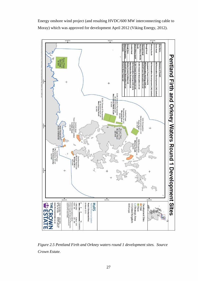
27

Energy onshore wind project (and resulting HVDC/600 MW interconnecting cable to

Moray) which was approved for development April 2012 (Viking Energy, 2012).

Figure 2.5 Pentland Firth and Orkney waters round 1 development sites. Source

Crown Estate.

28

In addition, there are various plans throughout Scotland to reinforce the electrical

network. A brief list of these include: Knocknagael (a new substation to allow 125

MW of export in the north west), a new 275 kV south west Scotland transmission line,

and upgrades to the following lines: Beauly-Blackhillock, Beauly-Dounreay, Beauly-

Mossford, Kintyre-Hunterston, East Coast transmission route (to 400 kV) and Scotland-

England interconnectors to increase the export capacity to 3.2 GW (Scottish Power

2011, Scottish & Southern Electricity, 2011).

Another disadvantage for all renewables is grid connection charges. A variation in

connection charges exists, due to losses in power that are incurred when electricity is

transmitted on the grid over long distances. The system to regulate this is continually

debated, and may change with Ofgem’s project TransmiT (Ofgem, 2011, Ofgem, 2011,

2, and Ofgem, 2012).

At present, a location dependent measure reflects the higher loss levels with the

increasing distance to demand, that is, high charges are imposed on those projects

furthest from the market. The National Grid charging zones have significant

implications for the location of renewable generation, as the preferred connection zones

are in the south closest to demand, which is unfortunately, furthest away from a

significant proportion of the marine energy resource. Therefore the charging system, by

default, imposes the highest charges on the areas with the highest renewable resource.

In areas with lowest resource/closest to demand, there are often no or negative

connection charges.

It is likely that the continual growth of onshore wind power (which also experiences the

best resources in remote areas) may help overcome transmission problems, and efforts

could also be made to look at other methods to avoid connection problems and charges,

such as producing hydrogen by electrolysis, i.e. allowing a product to be exported by

batch from a marine energy farm instead of exporting electricity directly to the grid.

In some remote areas it may be more logical to concentrate on supplying local demands,

rather than looking at expensive transmission to the central belt. It is also interesting to

speculate as to how much upgrading the grid actually requires. An integrated overall

upgrade of the system in the future (with the above mentioned AMS methods) could

see an efficient and cost effective result considering that traditional power plants do not

29

need to produce as much power if renewable energy producing to remote sites is

successful. However, there is no question that the remote outposts need upgrading to

allow generation to be exported, rather than being at the end of the import line.

The grid infrastructure is vitally important to the development of marine renewables

within the study area, and is therefore included within the model. The method used to

model the grid was a comprehensive list of coastal power stations and connection

points. There are also many inland power stations on the grid that are not particularly

relevant for the offshore modelling (such as offshore cabling to a development site),

however these will be important for the construction of onshore grid modelling.

The number of coastal Scottish power stations (and connections points such as EMEC

and oil terminals) is 31. Since the boundary of the project extends to include northern

England and the northern area of Ireland, the power stations and connection points from

these areas are also included to stay consistent with the other datasets the model used,

such as resource. Therefore, this figure is increased to 91 connection points from within

and around the study area.

Many of these connection points have limited capacity, however these will still play an

important role within the model, as the methodology allows real values (such as

capacity) to be altered to witness potential distribution changes. Conversely, by

following this methodology the model has the capability to determine what part of the

grid needs upgraded for certain developments to be undertaken.

2.1.3 Ports

Scotland has a wide range of ports, and unlike the grid infrastructure, large safe ports

are located strategically close to the actual resource. The Northern Isles is probably the

best example of this where good tidal and wave resource exist in combination with ports

such as Scapa Flow and Lerwick, which are more than capable of accommodating the

type of vessels/rigs required for marine energy deployment (Marine Publications

Limited, 2006 to 2011).

Ports around Scotland will play an important role in the development of marine

renewables and will likely have a bearing on the economics of a site development.

30

Therefore, datasets were required for ports and harbours in the study area, and along

with power landing points, make a significant contribution to the methods used by the

research model. The methodology behind the data capture, structure and storage was

similar to that of the power stations and connection points.

In conclusion 165 Scottish ports and harbours have been identified. Many smaller

harbours are also included, as although too small at present in terms of the size of vessel

they can accommodate, they may in the future be upgraded which highlights another

important aspect of the model. If a harbour is developed, the model can analyse

whether this will affect the cost of a MEC deployment, which if turned the other way

around, the model can show which ports should be developed.

2.2 Marine Energy Devices (MECs)

There are various forms of technology emerging in the marine energy sector as various

parties try to produce a device that will not only convert marine energy efficiently

within a construction and operational budget, but also withstand the harsh operating

environment. There has been a substantial amount of work done in the two distinct

sectors of wave and tidal technology, with major progress in both sectors in recent years

(RenewableUK, 2011).

The wave sector has a longer development history than tidal. However, this does not

relate directly to the advance of the two forms of technology in comparison with each

other. When many of the wave methods that are included within the research were in

development, tidal barrage was the only recognised form of tidal technology, a method

which in many senses is considered to be a different sector to tidal current technology.

Tidal current technology has advanced quickly and arguably has caught up with wave

development, if not surpassed it. From the initial study undertaken to formulate the

technological review for this research, a wider range of wave than tidal technologies

were found.

One explanation for this is the wave sector has been around longer, allowing a wider

range of methods to be developed within this greater length of time. Another (more

technical) reason is that the wave resource is much larger with many variations of deep

and shallow water waves which are very dependant on location. This has resulted in

31

various development methods, which are designed to extract, at most, only a very small

percentage of the energy in a very specific way.

Therefore, of the two distinct branches of the marine energy the wave sector has

developed a diverse range of devices and classifications, simply because there are more

ways to extract wave energy. There are schools of thought that believe this broad

diversification is a problem for the wave industry (Whittaker and Folley, 2005). There

is also a range of fringe products that have reached (or are very close to) commercial

status. These niche products have focused on other “work” that marine energy can

provide where other conventional methods are expensive. A short overview of this

technology is described within this section.

Tidal extraction methods on the other hand have had a shorter time to evolve, and have

the advantage of extracting a resource which is more consistent than localised wave

regimes. This has resulted in a common design theme that mainly resembles

underwater wind turbines, albeit with specialised alterations. In stating the above there

are of course a couple of exceptions to this rule with a handful of devices that use other

means.

Although MEC technology generally looks at a marine resource to produce electricity, it

is worth pointing out that some of the devices have actually been designed to perform

other purposes. The majority of devices included (in addition) will be able provide

potable water through reverse osmosis, or produce electricity as a primary resource or

for the purpose of producing hydrogen. Some devices are also designed in such a way

to act as a coastal defence as a secondary effect of extracting energy for one of the

above main purposes. All devices discovered within this research are included where

possible, as all are able to produce electricity even although their main purpose may

have been to fulfil other functions.

2.2.1 Technological review

One initial task set within this overall research was to identify the various forms of tidal

and wave technology and to provide a detailed evaluation of current and emerging

technology. A stand alone report was produced which provides a more in-depth

analysis of the industry and technology past, present and possible future, which cannot

32

be incorporated within this thesis because of page and word constraints. However an

electronic copy has been included within the accompanying DVD data which is

explained at Appendix K.

The technological review in itself can be used as a current reference on MEC

technology. The review has already been updated several times since the initial review

was completed early in the research. Behind the review the technical data were

captured in the relational database that is used by the model.

The majority of the material contained is directly from specifications and literature

released by developers. Significantly crucial information may be kept confidential and

the data (notably surrounding output and economics) in many instances have not been

verified by a third party.

The review therefore incorporates both wave and tidal technology and includes 76

devices, with a further 30 having been identified and logged in the main database,

however for reasons relating to insufficient technical data these are not processed by the

model. As a break down there are 45 wave devices and 31 tidal, with a further 24 wave

and 6 tidal identified but not presently used. With insufficient data this is not a major

concern as when the data do become available then they can obviously be included.

Historical device designs were also researched as part of the review, and added to the

database for completeness. It is also worth noting that the model may actually find a

historical design theoretically suitable at a given site. A full list of all the devices

included within this research is given in Appendix I.

One of the main conclusions from a previous springboard study was additional sites

may have been considered feasible, and better matching criteria may have been

identified, if additional forms of technology were reviewed (Wemyss, 2004). With this

in mind, it was deemed essential that the review included a broad view of past, current,

and emerging technology.

2.2.2 Wave energy and devices

Existing wave power devices can be categorised by several different methods: the

design used to harvest energy from the wave, the size and orientation, the intended

33

location, and by the power take off. The intended location includes shoreline and

offshore, both of which were covered in this research. The offshore category can then

be broken into two further sections: nearshore, and true offshore where a device would

extract energy from the wave in deep water around ≥50 m. The reasons for the differing

locations are described later in more detail.

If the size of device is very small compared to the typical wavelength, the device is

described as a point absorber according to a device’s horizontal size and orientation.

Conversely, if the extension is comparable to, or larger than the typical wavelength, the

device is called a line absorber, with the descriptive terms terminator and attenuator

being more frequently used. A device is described as a terminator or attenuator if it is

aligned along or normal to the prevailing direction of wave crests respectively (Brooke

2003).

Designs that attenuate the wave may be classified in various ways, for instance:

oscillatory motion, type of absorber, and type of reaction point. Energy can be absorbed

by the heave (vertical motion), surge (horizontal motion in the direction of wave travel),

pitch (angular motion about the wave crest), yaw (angular motion about a vertical axis),

or combinations of these.

The conversion of wave energy to usable power relies, in all cases on the effect of the

wave’s force on some material or fluid, be that a moveable mechanism or for instance

air or hydraulic oil. Three fundamental approaches can be set out from this within

which all wave energy devices fall:

Water to air interface. By allowing the wave action to enter a hollow structure

(which has an air chamber above a movable body of water) the wave forces the air

to move through an air turbine. The turbine then drives an electrical generator.

Water action on movable bodies. The wave action causes heaving, yawing,

surging and/or pitching motion of a solid or flexible body (or linked bodies). This

motion acts on a pump, forcing fluid through a hydraulic turbine or motor.

Water storage method. Waves are channelled along a tapered waterway where sea

water is lifted into a confined basin (reservoir) above the normal sea level. The

water is then released back to the sea in a controlled sluiceway through low head

hydro-electric turbines.

34

Power take off systems are required as a secondary conversion and are almost always

required to obtain useful form of energy. Methods include hydraulic rams and various

hydraulic and pneumatic components. Typically, secondary energy conversion is

obtained by means of a turbine. In addition, electric generators are included if the

absorbed wave energy is to be converted into electricity (Brooke, 2003). An example of

how PTO systems work together is the operation of the Aquamarine Oyster. Oyster's

hinged flap, pitches backwards and forwards in the nearshore waves. The movement of

the flap drives two hydraulic pistons which push high pressure water onshore via a

subsea pipeline to drive a conventional hydro-electric turbine (Aquamarine, 2012).

2.2.3 Wave devices coastal (fixed) methods

Devices that are fixed to, or embedded in the shoreline have a major advantage in that

maintenance and installation is much less complicated. In addition they do not require

deep water moorings and long lengths of underwater electrical cable to the shore.

However, these devices experience a much less powerful wave regime. The reason for

this can be explained by studying the behaviour of a wave as it comes ashore. In short,

water particles within a deep water wave move in diminishing orbital paths to a depth of

approximately ½ the wavelength below the still water level (Duxbury & Duxbury,

1993). Therefore, the radius of the orbit reduces exponentially with depth and as an

approximation, 95% of the energy is contained in the top ¼ wavelength of sea depth.

By the time waves come ashore they have already lost the majority of their energy due

to the interaction with the seabed as the water depth decreases.

This interaction occurs as the water depth decreases, this causes the particle motion to

change and frictional resistance to appear. The wave forms slow down and become

shorter, higher and steeper. The waves break when the steepness reaches 1/7. This

usually occurs when the water depth is around 1.3 times the wave height. Therefore,

most of the energy contained within the wave is released in the surf zone when the swell

reaches shallow water (Open University, 1999).

This means there are very few sites around the world where coastal forms of wave

extraction can take place. The main criteria for an onshore coastal method is for deep

water up to the shoreline, or a shoreline that can be modified or used to build an

35

extraction method. There are of course many cliff sites that will have deep water close

to the shore but it is then extremely difficult to house the extraction technology that is

required to convert the energy. Another method is to create an environment that can

house a conversion method, such as a harbour breakwater.

2.2.4 Wave devices offshore methods

The greatest wave resource is offshore before the wave interacts with the seabed and

shoreline. Offshore methods can be categorised into two distinct classifications:

nearshore and offshore.

The offshore class of device exploits the more powerful wave regimes available in deep

water (≥50 m depth) before energy dissipation mechanisms have had a significant

effect. Nearshore devices will be placed between the shoreline (but not fixed to) and

anything up to the 50 m contour (Brooke, 2003). There does not appear to be a clearly

defined distinction for when nearshore and offshore meet. In recent projects there has

been an indication by developers to install in water depths of around 70 m. This can be

seen with the new EMEC wave berth at Billia Croo, Orkney, and other projects such as

the Aegir project in Shetland, both of which are aiming for 70 m water depth (EMEC

2012, 2) (Aegir Wave Power, 2012).

Although the majority of the resource is offshore in deep water there are many good

reasons for choosing fixed coastal methods if a site exists, mainly due to the

survivability the device. Near and offshore wave devices have to operate in an

environment much more severe than fixed coastal devices. In order to extract energy

from the waves, the devices will need to be at, or near, the surface where the energy is

most abundant. Many devices are floating and require complicated and vulnerable

flexible moorings and electrical transmission cables (Brooke, 2003).

As there are limited sites available for coastal methods, offshore technology is being

developed in order to make large scale wave energy extraction become a reality.

36

2.2.5 Tidal energy and technology

Since the earliest days of seafaring and oceanography, it has been recognised that there

are strong sea currents with large amounts of energy. These are mainly caused by the

rise and fall of tides under the influence of the relative motion of the earth, moon and

sun’s gravitational fields. Useful energy has been extracted from the flow of water

currents for centuries, mainly in the form of water wheels or tide mills in rivers and

estuaries. A tide mill consisted of a pond filled through a sluice during the flood tide

and emptied on the ebb tide via an undershot water wheel. In more recent times tidal

barrage schemes using the same principle (to store water behind a barrage and thereby

storing potential energy) have been constructed.

Tide mills were in use around the coasts of Spain, France and the UK As early as 1100.

La Range Estuary was used as a Tidal Mill from the 12th

Century and the Schelde River

in Belgium was also used around 1800. They remained in common use for many

centuries, but were gradually replaced by more convenient methods of power

generation. The power was typically used for grinding grains into flour, the last

working mill in the UK (Woodbridge) was closed in 1957 after over 800 years of

service. Power was available for about two to three hours, twice a day. In Hayle,

England, tidal power was used to “dredge” a shipping channel by flushing it regularly

with a pulse of stored tidally impounded water (World Energy Council (WEC), 2001).

Tidal mill and barrage schemes use the height difference between high and low tide,

however, the flow of tidal currents can also be harnessed to generate power using

current turbines and hydraulic devices. Tidal energy (unlike most other forms of

renewable energy) can be predicted with high accuracy and the energy available for

conversion can be forecast with confidence.

2.2.6 Tidal barrage technology

Tidal barrage technology is a proven concept with the first (and still the largest)

example of a large commercial tidal barrage being the La Rance barrage on the Rance

estuary in Brittany, France. Construction began in 1961 and was completed in 1966.

The 22 km2 basin has a tidal range of 13.5 m (equinox tide) and the barrage across the

basin is 750 m long providing the towns of Dinard and St Malo with a major road

37

connection, thus saving a 35 km drive. The 24 x 5.4 m diameter turbines (rated at 10

MW each) can generate power during the flood and ebb cycle giving an overall rating of

240 MW. Annually La Rance produces around 600 GWh (EDF, 2010).

The smallest commercial tidal plant is located at Kislaya Guba on the White Sea in

Russia. It has a 500 kW capacity. There are approximately 10 other small barrages

scattered throughout the world, but they are not intended for commercial power

generation. For example, there is a 200 kW tidal barrage on the River Tawe in Swansea

Bay, that operates the gates of a lock. China has several tidal barrages of 400 kW and

less in size.

The second largest commercial scale tidal barrage was put in service at Annapolis

Royale, Nova Scotia, Canada in 1982. Annapolis utilises the sea water of the Bay of

Fundy home of the world's highest tides which can reach 17 m in height (World Energy

Council, 2001). Similar barrage schemes have been proposed in the UK at the Severn

Estuary (with a mean spring tidal range of 12 m) and Mersey estuary (with a mean

spring tidal range of 8 m).

A barrage scheme for the production of electricity at the Severn Estuary has been

investigated as early as 1925 with the establishment of a dedicated study group. In

1975 the Central Electricity Generating Board (CEGB) published a study stating a

barrage would not be feasible unless the energy situation deteriorated significantly

(Peters, 2010). In 1979 with the energy crisis the barrage was reinvestigated by the

Severn Barrage Committee which resulted in an energy paper recommending a 10 mile

barrage between Brean Down and Lavarnock Point (HMSO, 1981). This proposal was

investigated further by the Severn Tidal Power Group and in 1989 it was estimated the

barrage would cost £8 billion (generating 17 TWh of electricity per year) and was not

considered economically viable given the then present energy situation (HMSO, 1989).

The barrage was cited within the 2003 UK Government Energy White Paper as a future

possibility, although not considered fruitful to pursue at that stage (DECC, 2003, 2). In

2007 DECC through the Sustainable Development Commission concluded the project

could play a key part of the UK meeting its 2020 and 2020 CO2 emission targets

(DECC, 2011, 2).

38

At the beginning of the millennium detailed plans were emerging for the construction of

various tidal barrage plants in Korea, mainly the Shiwa (254 MW), Garolim (480 MW)

and Incheon (1 GW). Reports on the progress of these projects vary, although it is

evident the Shiwa project has been underway for some time as the original compound

was built for flood mitigation and agricultural purposes (Lee et al., 2006). An exact

completion date is unclear for the project as many target completion dates can be found,

most of which have passed. In circulation there are also planned completion dates of

2012 and 2015 for the Garolim and Incheon projects respectively (Korea Herald, 2010).

A barrage scheme can also forge a transport link across an estuary, which is beneficial

for the socio-economic environment. It also has the advantage of having a long

operational life with low maintenance costs, which can lower the economics of the

electricity production. However, large tidal barrage schemes do have major drawbacks.

Expensive initial civil engineering works are required which are usually lengthy, with

significant environmental consequences experienced in the estuary. These

consequences include:

Poor water quality.

Variations to water levels and, therefore, the inter tidal zones.

Disturbance to habitats and their ecology.

Violent sluice and turbine currents causing altered sediment distribution and

erosion.

During construction, major environmental impacts can also occur, for example, La

Rance Estuary was isolated from the open sea for 3 years during construction. There

are also a very limited number of sites around the world where large tidal barrages can

be constructed due to tidal conditions and geography. Various tidal barrage studies

have estimated that as little as 20 sites world wide may exist for large scale barrage

schemes (Hammonds, 1993). It is for all of the above reasons, tidal barrage technology

was not considered any further within this research.

2.2.7 Tidal lagoon technology

An alternative to tidal barrage technology is tidal lagoons, a new approach to offshore

tidal power generation that helps resolve some of the environmental and economic

39

problems associated with tidal barrage technology. Tidal lagoons use an impoundment

structure and low-head hydroelectric generating equipment situated offshore in a high

tidal range area. Shallow tidal flats having been identified as the most economical sites.

Although an alternative to tidal barrage technology, it is still likened to this method for

various reasons. This is mainly due to workings and construction of tidal lagoons.

They both suffer from one common drawback in that a substantial amount of capital has

to available, i.e. major engineering has to be carried out before any output is gained.

However, rather than blocking an estuary with a barrage, offshore tidal power

generators use an impoundment structure, making it completely self-contained and

independent of the shoreline, thereby eliminating the environmental problems

associated with blocking off and changing the shoreline. Although an offshore hazard is

created, navigation is not prevented and from an environmental point of view concerns

such as migratory fish will not be affected by isolated offshore structures.

Considering tidal lagoon technology is in a very early stage (in contrast to the maturing

tidal stream technology) the method was not considered any further within this research,

although a robust model would be able to determine suitable sites in the future with

more detailed information.

2.2.8 Tidal current technology

The kinetic energy within tidal currents can readily be harnessed with more simple

engineering concepts than compared to tidal barrage technology. Tidal currents usually

have a low velocity, however, when these movements are channelled through

constraining topography, such as straits between islands, shallows between the open

sea, and around the ends of headland, the tidal velocity is increased.

Probably one of the biggest milestones in tidal power was the realisation that turbines

(similar to that of designs to work in air) would work in water. The main advantage of

this, is that tidal development was able to move forward quickly using experience

already gained in the now more mature wind sector. It is for this reason many devices

resemble underwater turbines, with a few exceptions.

40

Although tidal devices operate in a relatively stable location the environment is still

technically challenging. Any mechanical device does not generally like to be exposed

to seawater, and electrical equipment is (by its nature) averse to moisture. The high

density of water (around 832 times denser than air) means that devices are exposed to

large forces acting on their structures from both the movement of the tides and the

effects of surface waves, especially if surface piercing. By definition, they also must be

installed in areas where high current velocities are present, where tidal windows (slack

water) are very short, contributing to difficult installation and maintenance operations.

2.2.9 Description of relevant devices used in modelling

The technological review describes all the identified wave and tidal devices in full.

There is also a discussion document detailing an alternative categorisation method of

these devices in terms of their marine placement. These documents are located within

the “Write up and associated files\Technological Review” folder on DVD disc 1.

To save the reader referring to the technological review within the DVD, a summary of

the devices relevant in this thesis are described below. These are the devices that are

important to the modelling results later in the thesis.

Wave Dragon

Wave Dragon is an offshore wave device that has a large reservoir contained within the

structure. This reservoir is filled by waves overtopping the structure, channelled by 2

wave reflectors towards a ramp where the water is elevated and released at the base of

the structure via turbines. The device is buoyant and is tethered to the seabed. The

device is referenced in the model as Device 4.

Pelamis

Pelamis is an offshore wave device which consists of four long cylindrical sections

linked together by three hinged joints containing three hydraulic independent power

conversion units. The device is tethered to the seabed, is buoyant and floats on the

surface where the relative motion of the different segments of the device, as it contours

the surface, provides the power. The device is referenced in the model as Device 5.

41

OSPREY

The OSPREY (Ocean Swell Powered Renewable EnergY) design is a nearshore wave

device. The power take off system is an Oscillating Water Column (OWC)

housed in the buoyant device that is ballasted to create a gravity base on seabed. The

device is referenced in the model as Device 7.

Wave Star

The Wave Star is a nearshore wave device based on a row of floats, with integrated

arms, which are fixed to a horizontal shaft with a one way bearing. The device is held

on station by the structure penetrating the seabed. The device is referenced in the model

as Device 13.

PowerBuoy

PowerBuoy is a nearshore wave device that uses an internal piston that moves as the

buoy heaves with the rise and fall of the waves, and in turn driving a seabed generator.

The device is buoyant and tethered to seabed. The device is referenced in the model as

Device 26.

Marine Current Turbine

The Marine Current Turbine (MCT) is a tidal stream device using a pair of axial flow

rotor turbines. The nacelle (with turbines, gearboxes and generators) is mounted on a

monopole that penetrates the seabed. The device is referenced in the model as Device

46.

TidE1

The TidE1 is tidal stream device using a pair of contra-rotating turbines mounted

together on a single crossbeam. The nacelle contains the gearbox and generator. The

turbines are of an axial flow rotor design with an assembly which is buoyant and is

fixed (submerged) to the seabed using a flexible wire mooring arrangement. The device

is referenced in the model as Device 47.

42

Hammerfest Strøm

The Hammerfest Strøm is a tidal stream device. The nacelle contains the gearbox and

generator. The turbines are of an axial flow rotor design. The bottom mounted base is a

steel structure with gravity footings made. The device is referenced in the model as

Device 56.

Tidal Generation Ltd

The Tidal Generation is a tidal stream device. The nacelle contains the gearbox and

generator. The turbines are of an axial flow rotor design. The bottom mounted base is a

steel structure with gravity footings made. The device is referenced in the model as

Device 64.

Test wave device and test tidal device.

The test wave and tidal devices are set within the model to have favourable attributes to

allow the model to be tested. As for design they are assumed to use an Oscillating

water column (test wave) and water turbine (test tidal). The devices are referenced in

the model as Device 75 and Device 76 respectively.

43

ID Name Type Depth Resource Distance Output

4 Wave Dragon Wave 30 m 48 kW/m Null 11 MW

5 Pelamis Wave 50 m 27 kW/m 5 km 0.75 MW

7 OSPREY Wave 14 m 25 kW/m 0.3 km 2 MW

13 Wave Star Wave 15-20 m 10 kW/m Null 5 MW

26 PowerBuoy Wave 30 m Null Null 0.02 MW

46 Marine Current

Turbines

Tidal 50 m 2.83 ms-1 Null 1.2 MW

47 TidE1 Tidal 30-200 m 2.57 ms-1 Null 1 MW

56 Hammerfest Strøm Tidal Null 1.8 ms-1 Null 0.35 MW

64 Tidal Generation Ltd Tidal 20-100 m Null Null 1 MW

75 Test wave Wave 5-200 m 27 kW/m 100 km 1 MW

76 Test Tidal Tidal 5-200 m 2 ms-1 30 km 1 MW

Figure 2.6 showing a summary of devices that feature in the data modelling and

analysis later in the thesis. These parameters within the database are key to the

calculations of the model. Values that are unknown (Null) will not allow the model to

consider the devices beyond the initial stages of testing. The reason these devices do

feature in the more detailed modelling is because these values are updated in the model

testing in Chapter 5 of the thesis.

44

CHAPTER 3 – DATA REQUIREMENTS AND MODEL DESIGN

This chapter describes in detail the design and data requirements of the model, and is

structured to reflect the sequence of steps undertaken:

Initially a generic dataset review was conducted to identify the data required to

construct a model to satisfy the aims of the research, (3.1 to 3.3).

Following the initial data review, a top level model design was developed, (3.4).

After discussion, a top level design for a working example of the model is

presented, recognising there was neither time, nor available data to construct the

ideal design, (3.5 to 3.6).

Before a more detailed design could be finalised, a closer look at the available

datasets was required to give a clear description of the inputs, outputs, data

structures and how all of these interact, (3.7).

The available datasets identified required manipulation which is documented, (3.8).

Leading from the full data description and manipulation, a more detailed working

model design with the model data flows was developed, (3.9).

To conclude the chapter, a review of the model testing methodology is documented,

(3.10).

At the earliest stage of the design it was envisaged that the project would have data

requirements that fall into three distinct forms: 1) External datasets, 2) Self constructed

datasets, and 3) Automated model datasets.

3.1 External datasets

The boundary of the project was defined early in the project as a relatively wide area,

with coordinates up to 61.5° to 54° north / 9.75° west to 3.375° east. Considering this

geographical range and the time scale that was involved, it was impossible to manually

construct data for this region, or if so, it would not be at any kind of resolution that

would be helpful. Therefore, to save time (and in many respects to increase accuracy) it

was deemed essential that data be sought for many of the model parameters.

In the early stages of the project it was difficult to determine exactly what data would be

available, however, it was clear the model would require resource data (wave and tide)

45

and bathymetry data in order to conduct the most basic of site analyses. For more

complex and accurate analysis various constraint datasets would be required. An

idealised list of datasets (and potential sources) for a definitive site analysis was

developed as follows:

Resource data such as wave, tidal, and wind. Sources: DTI, Seazone.

Bathymetry. There are various water depth datasets available from various sources

such as: International Hydrographic Organization (IHO), UK Hydrographic Office

(UKHO), GEBCO, SeaZone, DTI.

Other physical data such as geological data to confirm the condition of the seabed

and so on. Sources include British Geological Survey (BGS), UK offshore oil and

gas information (UKDEAL), SeaZone.

Areas of high vessel density associated with narrow channels and shipping. Various

data sources available: Automatic Identification System (AIS), marine radar and

traffic systems.

Offshore structures such as in the oil and gas industries and their associated

pipelines, safety zones and so on. Sources: UKDEAL, SeaZone.

Offshore electrical and telecommunication cables. Source: UKHO.

Wrecks and other marine archaeological sites. Source: UKHO.

Former dumping grounds and contaminated areas. Source: UKHO.

Military zones such as training areas and bombing ranges. Source: UKHO.

International shipping lanes and areas of high vessel density. Sources: International

Maritime Organization (IMO), AIS.

Fishing grounds and aquaculture. Sources: Marine Scotland and Crown Estate.

Offshore wind (various deployments and leasing rounds), and of course other MEC

developments. Source: Crown Estate.

Other activity areas and licencing. Source: Crown Estate.

Other marine resource extraction such as marine aggregate dredging.

Areas of high recreational use.

Protected and special sites, such as: Special Protection Area (SPA), Sites of Special

Scientific Interest (SSSI), and Special Areas of Conservation (SAC), National

scenic areas, RAMSAR (Convention on wetlands) sites, Marine Nature Reserves

(MNR), National and Local Nature Reserves (NNR/LNR). Sources: Crown Estate,

Scottish Natural Heritage (SNH), Marine Scotland.

46

Areas close to protected sites where the designation includes mobile species such as

seals and birds.

Other environmentally valuable sites (that are not officially designated), such as:

maerl beds, reefs and so on.

Breeding areas for: birds, seals, cetaceans and fish such as herring spawning areas.

3.2 Self constructed datasets

A high percentage of the data that was specific to this project had to be sourced and

compiled.

An initial task was to conduct a review of the past and present wave and tidal

technology. This allowed the required knowledge of the technology and the industry as

a whole to be gained. It also allowed the construction of a database (logging each

device) with any known associated data to be used in the program model. For the

model to operate effectively, device data (such as the rated output, depth constraints,

resource constraints, core construction materials and so on) were all fundamental

attributes for the various model algorithms. The devices that are important, in terms of

model testing for this thesis, are detailed above at 2.2.9 Description of relevant devices

used in modelling.

After assembling the device dataset from the review, similar datasets began to be

produced. These datasets were for: ports, coastal power stations, offshore cable types

and so on. These were essential to the project, and although easy to construct with

publicly available data, it was a time consuming task.

To source the actual data, various methods were used. Most of the searches would

normally start on the Internet which would usually give an indication where information

was available. For the port dataset for example, data were obtained from a variety of

sources, the port’s own information on the Internet and handbooks, Admiralty charts,

Google Earth, pilot handbooks, tide tables and atlas. This allowed various data fields to

be populated, such as: water depth, quay lengths/locations, tidal ranges and times,

maximum ship dimensions, port services and so on. More often than not, each source

provided a little piece of the jig saw required to complete a useful dataset.

47

The self constructed datasets comprise:

Devices: containing their type, specifications, output, weight, Power Take Off

(PTO) type, and cost.

Power Take of Systems (PTO) and their costs.

Material types and their costs.

Mooring types and their costs.

Cables type: containing their design, specifications, and costs.

Power stations/electrical landing points: containing thier locations, spare capacities,

connection charges.

Ports: containing their locations, capabilities and cost.

Ships: their specifications and costs.

3.3 Automated model datasets

The third category of data that is used within the program model was data that were

constructed automatically by the program itself. Working with the two other data

collection methods described above, the model is designed specifically to have the

functionality to construct new datasets from these existing datasets, i.e. perform a set of

tests or calculations and print the results to a new dataset. In a cascading effect the

newly constructed data are then used again for further analysis, which may produce

further datasets, and therefore continuing the data development process. As one

example, the program model has to be able to take every given location, calculate the

distance to the nearest power station, and store this distance and station id at each

location to a new dataset. Then, for any given location, this newly constructed dataset

with the distance values is used to calculate a cable type, again storing the results, which

are then used to calculate a cable cost and so on. The model produces a substantial

amount of data by this method.

When the model program produces a new dataset, it is in the form of a matrix, with the

data spatially arranged within the area of the project boundary, and in the same format

as the externally sourced data which are then used for comparison and computation.

This functionality allows single values such as latitude and longitude in other datasets

such as list tables (for example a database table containing only a name of an entity and

its location) to be used by the program model to construct distance matrixes to the

48

spatial boundary of the project. This design methodology allows spatial data to be

quickly and easily constructed.

3.4 Top level design for the model with the identified datasets, and project aims

Once the general input datasets had been identified, the top level design for the model

was developed. From the identified input files a structural flow chart was constructed

to help understand how these datasets interact with one and other, and what parameter

values can be determined.

At this stage, the design followed the logic that each process (a labelled text box within

a structural flow chart) would carry out a specific task which allows the model to

progress, firstly to find a valid site result for each device (to satisfy the site selection

aim of the project) and then to a final profit/loss indicator for that site. This design

assumes a dataset of devices will sit around the described set of sequences, and

therefore each device is tested in sequence (with each process detailed in the flow chart)

to determine where it can be located, and give a profit/loss indication for that site.

49

Figure 3.1 showing a top level design for what is required to satisfy the aims of the

model. Most of the processes have been simplified (grouped into higher level single

processes) for this level of design. The blue arrows represent the site analysis aspect of

the design, while the green ones represent economic aspects.

1Test external physical

constraints

12 Potential

ROCs etc

5 Determine

spare capacity

9 Device cost

8 Number of

devices/output 6 Determine cable

type

21 Entire

Project cost

11 Running

costs

15 Depth

factor

22 Determine

profit/loss

13 Calculate

revenue

14 Distance

from port factor

4 Find shore power

station/ distance

2Test other external

constraints

7 Cable cost

17 Installation

cost

10 Maintenance

costs

19 Physical

project cost

20 Financial

costs

3Valid site

16 Weather

factor

18 Decommission

cost %

50

The design (shown in Figure 3.1) it not intended to describe how this model works.

Furthermore most, if not all, of the above processes require complex code and data

structure management to achieve their specific aims, and also require design

methodologies at much lower levels from this the top level design. However, in the

following text, the top level design is explained and is expanded to show how the lower

levels of the model were built up around it.

3.5 Overall description of the program model design

In order to process the considerable amount of data that were required for this project,

the most feasible approach was a batch sequential computer program, where the

program takes each device in turn, and works matrix cell by cell from the north west

boundary (working east) line by line (south) through the external data conducting the

various tests required. With this design, the model is able to process every device with

every site during the one single program run without any user intervention.

3.5.1 Finding a valid site

It can be seen from Figure 3.1 that many of the processes are complex, and require

multiple calculations to take place.

During the initial processes (indexed 1 and 2 in the flow diagram) the device will have

to pass various tests to ensure the device is suitable for the site. There will be many

physical tests such as resource, which will restrict all devices if not favourable. After

all, no energy converting device can be deployed in an area with no or little resource.

There is also an upper limit to this of course where the resource may be too extreme.

There will be other restrictions such as shipping or scenic areas that are not so clear, and

could be device specific. For example, some devices are on the seabed and others will

have structures piercing above the water column. Another potential restriction is the

presence of offshore structures such as in the oil & gas industries. For most devices this

will be a restriction, however a very small number of devices may actually be able to

work in conjunction with these structures (for example providing a fixing point in deep

water with electrical infrastructure) and would pass this test at this location, where other

devices would fail.

51

Each device will require substantial information to be known in order for a valid site

(index 3 on the flow chart in Figure 3.1) to be found. In fact, the list is determined by

the number of external datasets that can be obtained or constructed. Therefore, the

processes and associated datasets required to undertake the physical constraints test

(index 1) use the following design format:

Figure 3.2 showing an expanded view of the likely physical constraints (and therefore

datasets) that the device is tested against at every site.

For testing other external constraints (or non physical external constraints, at index 2 of

the flow diagram) a very similar method was applied with various additional constraint

datasets being used:

Test external physical

constraints

Distance

to land

Wrecks Resource Offshore

structures

Military Geology Water

depth

Training Bombing

ranges

Platforms

oil/gas Oil/gas

exclusion Wind/other

MECs Pipelines Cables

Electrical Communications

Wave Tidal

Combined

analysis

Dumping

Grounds

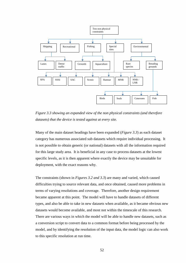
52

Figure 3.3 showing an expanded view of the non physical constraints (and therefore

datasets) that the device is tested against at every site.

Many of the main dataset headings have been expanded (Figure 3.3) as each dataset

category has numerous associated sub datasets which require individual processing. It

is not possible to obtain generic (or national) datasets with all the information required

for this large study area. It is beneficial in any case to process datasets at the lowest

specific levels, as it is then apparent where exactly the device may be unsuitable for

deployment, with the exact reasons why.

The constraints (shown in Figures 3.2 and 3.3) are many and varied, which caused

difficulties trying to source relevant data, and once obtained, caused more problems in

terms of varying resolutions and coverage. Therefore, another design requirement

became apparent at this point. The model will have to handle datasets of different

types, and also be able to take in new datasets when available, as it became obvious new

datasets would become available, and most not within the timescale of this research.

There are various ways in which the model will be able to handle new datasets, such as

a conversion script to convert data to a common format before being processed by the

model, and by identifying the resolution of the input data, the model logic can also work

to this specific resolution at run time.

Test non physical

constraints

Fishing

Shipping Special

sites

Environmental Recreational

Rare species

Breading

grounds

SPA SSSI SAC Scenic Ramsar

Cataceans Fish

Lanes Dense

traffic Grounds Aquaculture

Seals Birds

MNR NNR /

LNR

53

For the model design when more than one valid site is found, there is then the need to

compare the adjacent sites as they may have a hydrodynamic effect on one another.

That is, a decision will have to be taken as to how many devices will be allowed at any

particular site. For example, when a tidal device is placed downstream of another

device (which of course becomes upstream once the tide has turned) each device will

experience a modified resource. The downstream resource will be less as some of the

energy has already been converted by the upstream device(s) and the structure shape

and operation is likely to cause turbulence in the water column. For wave energy this is

similar with offshore devices likely to affect devices between the further offshore

deployments and the shoreline. Again, this is likely to be a reduced (and distorted

quality of the) resource.

Therefore, multiple valid sites need to analysed to determine the effect of spatial

placement, and sites (along with the total allowed number of devices at any given site)

may need to be reduced if they are deemed to potentially cause a problem. There is

little known about the possible effects of multiple devices in close proximity, as to date

deployment of device arrays has not been achieved. There can however be estimations

drawn from similar studies, such as Wind Park Effect for the spatial distribution of wind

arrays.

The results of such calculations will feed into the economic calculations of the model

(index 8 on the flow chart in Figure 3.1) in terms of how many devices will be placed at

a site, and therefore the site output. At this point a suitable load factor for each device

will be determined. This value (in megawatt hours MWh) will have to take into

consideration the individual device design load factors with the largely unknown

packing densities, so will be initially set low in order not to over estimate. A key

feature at this point is the ability of the design for these values to be calculated more

accurately in the future, by using key user defined variables in the database, as

knowledge is gained. There is a further discussion of packing densities at Appendix A.8

Calculate the number of devices required and device output at a given site.

54

Figure 3.4 showing an expanded view of the more detailed site analysis incorporating a

hydrodynamic modelling element.

The above can only be achieved by incorporating a hydrodynamic model to determine if

certain sites will cause a problem, which may in turn modify the number of valid sites,

i.e. potentially more sites eliminated as the model essentially creates another constraint

to be overcome. The reason this hydrodynamic consideration is incorporated separately

from the other constraints (that is, the hydrodynamic analysis is not an extra constraint

test carried out at the same time as the other constraint analysis) is because the entire

valid sites dataset has to be completed first. Valid sites have to be found so a

comparison can take place. This cannot be done during the constraints analysis, as this

increments one site at a time and the overall valid sites (index 3 in Figure 3.1) is only

complete at the end of the constraints batch procedure, meaning combined valid site

analysis can only take place after all the valid sites have been found. To help the logical

operation of the model, the resource datasets would likely be altered by the

hydrodynamic feature at run time for each device each time a valid site was found.

3.5.2 Determine a cable, costs and revenue

Once the valid site (index 3) is found, the model determines the closest land power

station/power landfall point. This is done by comparing the location of each site, and

the location of each recorded landfall point in a separate dataset, which also holds the

Union of sites that pass all constraints

Updated union

results/valid sites

Hydrodynamic study

of multiple valid sites Comparison of valid sites

Valid Site

No of devices/output

Find shore power

station/ distance

55

spare grid capacity of this landfall point (covering indexes 4 and 5 on the main flow

chart). If this landfall point does not have enough capacity (which maybe for various

reasons, such as bottle necks exporting the energy on land, Beauly-Denny in the North

of Scotland for example) the next closest landfall point has to be found. Storing (and

testing) data such as power landfall points without any capacity, is as important for the

working of the model as landfall points with capacity, as it may be able to show where

bottle necks are, and therefore where development is required. Another way to look at

this would be to say, what if we entered a “landfall” connection point in the required

dataset to be somewhere offshore, i.e. in an area where there are currently only long and

expensive distances to shore facilities. The model would then be able to test this

connection point which may positively affect the amount of available sites, and would

most certainly change the economics of these sites and therefore the overall spatial

distribution.

It is clear the model has to be setup in such a way where connection points and/or

associated capacity values can be changed to show any distribution changes. It was

therefore a design requirement that as many values used by the model for calculations

could be altered for the purpose of analysis.

Knowing the spare capacity and distance to landfall allows a cable type to be

determined, index 6. There is a significant amount of logic required for cable selection,

with a further dataset containing the various cable types depending on distance, and

rating. Distance is assumed to be a key variable for the selection of cable type, with

various configurations having an ideal minimum and maximum range that is used to test

against the distance to landfall point. The database has a cable configuration example

from the offshore wind industry, this has been used to define a working range which

may not give a true reflection for some MEC development scenarios. However this

range can be changed by the user as knowledge is gained. Once the single ideal cable

type (with associated rating) is determined by the model the number of devices (assisted

by the valid site analysis at index 3), the output of the site (and therefore overall revenue

via any potential financial incentives) as well as the cable and connection costs can be

determined, which covers indexes 8, 9, 12 and 13 of the main flow chart.

To determine the device cost (index 7) more information on what makes up the device

is required. The base materials, power take off (PTO), and moorings need to be

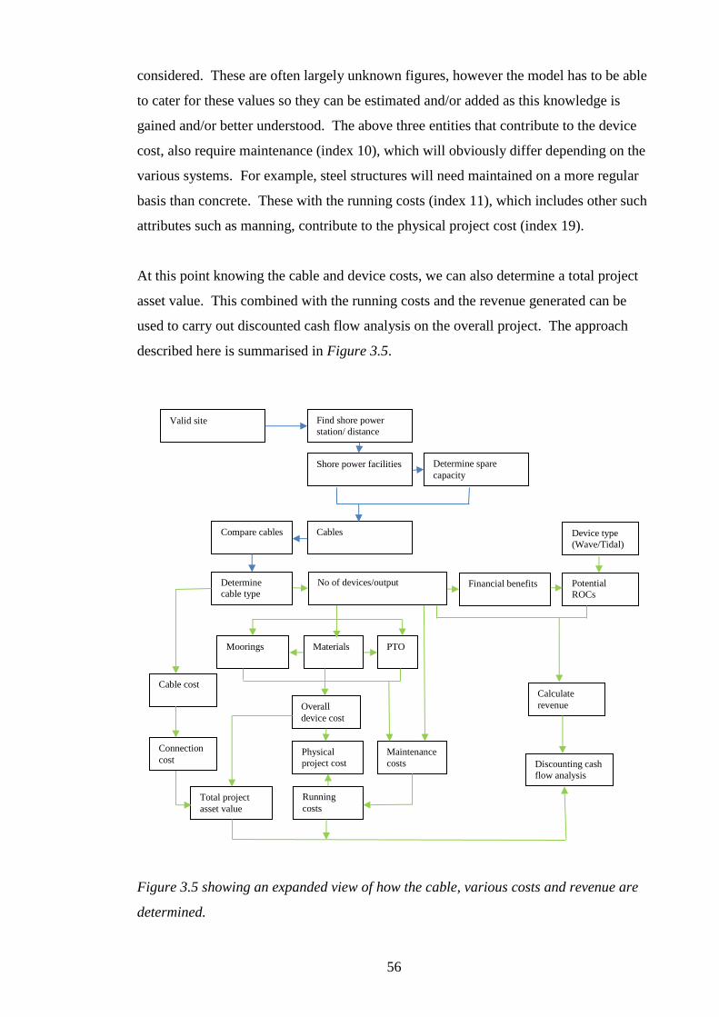
56

considered. These are often largely unknown figures, however the model has to be able

to cater for these values so they can be estimated and/or added as this knowledge is

gained and/or better understood. The above three entities that contribute to the device

cost, also require maintenance (index 10), which will obviously differ depending on the

various systems. For example, steel structures will need maintained on a more regular

basis than concrete. These with the running costs (index 11), which includes other such

attributes such as manning, contribute to the physical project cost (index 19).

At this point knowing the cable and device costs, we can also determine a total project

asset value. This combined with the running costs and the revenue generated can be

used to carry out discounted cash flow analysis on the overall project. The approach

described here is summarised in Figure 3.5.

Figure 3.5 showing an expanded view of how the cable, various costs and revenue are

determined.

Cables

Determine spare

capacity

Financial benefits No of devices/output

Find shore power

station/ distance Valid site

Shore power facilities

Determine

cable type

Cable cost

Compare cables

Potential

ROCs

Calculate

revenue Overall

device cost

Materials Moorings

Running

costs

Maintenance

costs Discounting cash

flow analysis

Total project

asset value

PTO

Physical

project cost

Device type

(Wave/Tidal)

Connection

cost

57

The detailed low level design and code for this section is substantial.

3.5.3 Determine installation, decommissioning and financial costs

The design work described in 3.5.1 and 3.5.2, provide the main foundations of the

model. However, a few more details complete the description of the overall design. To

complete the physical project cost (index 19), the installation costs (index 17) need to be

determined which is another complex problem. One of the main attributes that will

determine the installation cost for any particular devices is the geology of the site in

which the device will be deployed. The geological dataset can referenced back through

the hierarchy (as it was processed in the site analysis procedures) and will therefore be

known by cross referencing. Other factors will include the distance from port, water

depth, and weather windows covering indexing 14, 15 and 16 (see Figure 3.1) and for

each particular area the shipping costs. The distance from port calculations work in an

identical fashion to determining electrical landing points, so that computer code is

reused at this point. The water depth is already known as it has been processed during

the site analysis.

Weather factoring is slightly more complex and takes into consideration wave and tidal

resource at the site, and also wind. Not all sites are as exposed as others so this could

have a significant outcome to the overall profit/loss result, as it will have a bearing on

the ships and equipment used to carry out the installation, and weather windows for

maintenance.

As for decommissioning (index 18) this is another unknown but does work in a similar

(reverse) fashion to that of installation, so a percentage figure could be used together

with all the previous work described above to give an overall physical project cost, and

therefore an overall amount that can be used to calculate the finance (index 20)

required. This will in turn then give an entire project cost (index 21) which can be

directly compared to the revenue gained (index 13) giving a final profit/loss figure

(index 22). This approach is summarised in Figure 3.6.

58

Figure 3.6 showing an expanded view of how the installation, decommissioning, project

costs, and profit/loss are determined.

3.5.4 Conclusion drawn from top level design

Given there were many constraints encountered during this work, mainly research time

(to source, construct, format the various datasets identified above) and available

resource to purchase datasets that cannot be obtained publically, it was considered, at

the initial design phase, not possible to construct the model in its entirety. For example

to undertake the full valid site analysis, a detailed hydrodynamic model would be a

substantial undertaking as there is little knowledge at present on how devices will affect

one and other, which is a significant research topic in its own right.

Therefore, the strategy was to concentrate on a working representation of the model,

giving the best indication of how the overall structure would work with available time

and data. Unfortunately, sacrifices had to be made and it was not easy to decide how

best to demonstrate an overall working model from the ideal design described. That is,

what was to be built, and what functionality had to remain in the design. As already

mentioned, some of this was determined by data availability. However, some aspects

Entire project

cost

Depth

factor

Determine

profit/loss

Revenue

Distance

from port

Installation cost

Physical project

cost

Financial costs

Weather

factor

Decommission

cost %

Shipping costs

Water

depth Geology Wind Wave Tidal Ships/offshore

equipment

59

were too important to leave out, regardless of how difficult it proved to obtain the data

required.

3.6 Design analysis for working example of model

At this juncture it is worth noting what was left out of the model presented here and

why. Starting from the top the model design now only compares a device to: resource,

bathymetry and distance to land data, rather than the extensive constraints originally

designed. This is for several reasons. The data for all the identified constraints proved

difficult to obtain, and to verify the working of the model, logically, not all constraints

would be required. For the model design to process three constraints is logically the

same as processing a large number. It is also the case that the constraints analysis is one

of the less complicated features to add onto the overall program at a later date, as the

structure will be in place to import and process the additional constraint data.

From this point, rather than cut out key aspects of the design, the decision was taken to

simplify many of the processes. Again, this has been done to show an overall working

structure where the level of detail can be built upon at a later date. Therefore, the valid

site analysis and installation calculations are simplified, as are the running costs,

detailed financial analysis, ROC systems and so on.

After careful consideration a simplified design was reached to show an overall working

model from the earlier complete design. That is, an overall working model which

would provide a valid site per device and profit/loss indicator for that site, rather than

encompassing all aspects of the overall design. The design in Figure 3.7 details this,

with the processes at a design top level; again the lower level functionality is not shown.

As before, the design is based on a batch operation, running through each device in turn,

with each site, until all devices have been tested with all sites.

60

Figure 3.7 Top level design of overall ideal model, with dash sections showing what

was omitted from the example model top level design.

Test external physical

constraints

Potential

ROCs etc

Determine spare

capacity

Device cost

Number of

devices/output Determine cable type

Entire Project

cost

Running costs

Depth factor

Determine

profit/loss

Calculate

revenue

Distance from

port factor

Find shore power

station/ distance

Test other external

constraints

Cable cost

Installation

cost

Maintenance

costs

Physical project

cost

Financial costs

Valid site

Weather

factor

Decommission

cost %

61

Before a more detailed design description of the example model is presented, a closer

look at the available datasets (and how these were formatted) allows a clearer indication

of the inputs and outputs, data structures and how all of these interact.

3.7 Datasets selected to construct model

The requirements for the three already identified categories of datasets used: external

required datasets, self constructed datasets, and automated model datasets are described

in more detail.

3.7.1 Acquired external data

The main requirement after the design stage was to begin construction of the model and

provide a site analysis from oceanographic features such as the bathymetry, wave and

tidal resource. There are various sources where bathymetry data could be obtained for

the study area. Obtaining the resource data on the other hand was not so easy, there

were many specific studies in localised areas from smaller studies which have been used

to build up resource modelling, such as used by the DTI.

The DTI produced an atlas of the UK renewable energy resources in 2004 to document

the resource available for wave, tidal and wind energy. The atlas also came with a CD

ROM with the underlying data mainly in the database management format of dBase. In

terms of this project the data accompanying this work was invaluable as the resource

and bathymetry data can be extracted. The dataset gained from this source is listed in

full in Appendix A. This list also shows the dataset types and the value range of the

data entries. In the DTI CD ROM there are also some other very useful datasets,

“distance to shore” being one as various distance calculations were required in the

model. There are also 20 wind datasets which could have been used in the

installation/decommission costing in the model. However, this was scaled back in order

to save time and ultimately allow for a complete representation of the model to be

completed. These available datasets is a feature that can easily be added at a later date.

The digital DTI datasets also contained more data than appears graphically in the hard

copy of the atlas. Some of these have been used in calculations (for example to

62

calculate mean results from several underlying datasets) and were therefore not printed

in the atlas as stand alone sets.

There was slightly more choice when considering bathymetry data during the initial

data review. Publicly available bathymetry data were also acquired from the General

Bathymetric Chart of the Oceans (GEBCO) digital atlas. The GEBCO, one minute grid

data are freely available to download via a host at the British Oceanographic Data

Centre (BODC) (General Bathymetric Chart of the Oceans GEBCO, 2003). Therefore,

a copy of the north Atlantic data were obtained which was stored in an xyz format

within a text file. After the bathymetry datasets where selected and formatted for the

model, it was found that GEBCO had released a higher resolution dataset. This was to a

half minute resolution compared to both the approximate 1 minute datasets from the

DTI and previous downloaded set from GEBCO.

There is also bathymetric data available from SeaZone who sell digitised data from UK

Hydrographic office Admiralty Charts. This is a widely used resource and was

considered at the time of the data review. There were several concerns at the time with

the SeaZone data in comparison to the data that could be obtained from the

DTI/GEBCO.

SeaZone mainly vended data in localised zones, i.e. small geographical areas such as

found on shipping charts. To cover the area required the majority of the individual

Seazone sets for Scotland would have had to have been purchased. There were also

concerns regarding data processing such as joining the various zones to construct a

single dataset, and the use of techniques such as kriging to interpolate irregularly spaced

Seazone data to a required model grid, i.e. to ensure a populated matrix (at a defined

resolution) was made up from the distributed sporadic nature of Admiralty charted

depths.

Taking the data resolution discussions further it also became apparent that regardless of

the quality of resolution (around half minute resolution) gained by purchasing data,

there was a restriction from the resource data in any case. As the DTI resource data

were to be used for resource, therefore, potentially higher resolution bathymetry data to

run alongside the resource data were not going to enhance the model significantly, that

is, in relation to the cost of (and work required to format) the data.

63

The easy access to the GEBCO and DTI datasets, and the overarching aim of producing

a working example rather than a detailed section of the model, meant the SeaZone

datasets were not considered further.

As for the GEBCO data it was a similar story with the higher resolution half minute

dataset. There was the added disadvantage that this set only became available after the

DTI and lower resolution GEBCO datasets, which were selected for further modelling.

The GEBCO one minute dataset was the first dataset found with the initial data review

and after going through the various formatting processes it was decided to include the

GEBCO data alongside the DTI bathymetry data for two main reasons.

The two datasets (at slightly different resolutions described fully within sections

3.8.1 and 3.8.2) can be used to validate one and other.

One of the main design requirements is to develop a model that can handle data at

different resolutions. Therefore, the GEBCO data (in comparison to the DTI data)

will be used to test (and be an example) of how the model data structures are built

to handle this functionality.

3.7.2 Self constructed datasets review

For the self constructed datasets there has been little change with the model redesign.

All of the main datasets captured (with the exception of ships) are still used within the

model. However, some of the attributes within some of the main datasets are redundant.

The flexibility of the model to pick and choose the data to manipulate, allowing

additional data to be incorporated at a later stage, is maintained.

3.7 3 Automated model data

The third category of data used within the program is the data that are constructed

automatically by the program model itself. Therefore the new design and changed

outputs to the overall model will have little effect on these data structures, but with

reduced inputs there is proportionately less automated data produced.

64

3.8 Manipulation of available datasets

Once it had been established which datasets were to be used in the model, investigation

focussed on how these datasets were handled. Obviously there are various sources and

types of datasets, which required specific manipulation. All of the external datasets

were manipulated by various methods (sometimes several times) to enable storage in a

format that the program model could use.

The external datasets are obviously constructed by someone (or by a program designed

to produce a desired format by someone) and therefore required an initial analysis to

identify what this format was. Once the format was understood, the choice was then

either to construct program code to directly use the data in its original format, or

construct new code to reformat the data into a structure more appropriate to the overall

requirements.

3.8.1 GEBCO data

The GEBCO dataset was the first external dataset which was acquired. The initial file

was in a 1 minute resolution from 90° north to 90° south / 180° west to 180° east which

is the entire globe. The original file was 280 megabytes (mb) making it difficult to

work with, i.e. simple tasks such as opening the file was difficult. This task was made

more difficult in that the original file format was a UNIX Operating System variant

where there were various hidden characters that Windows could not decipher.

Therefore, a Visual Basic for Applications (VBA) script within MS Excel was

constructed to copy the contents of the file into another file recognised by MS

Windows. A further script was constructed to take only the data range required, and

again save this to a new file. The resulting file contained data from 65° north to 54°

north / 20° west to 4° east, as at this early stage of working the exact project boundaries

had not yet been fixed. The project boundaries were later defined once the DTI

renewable resource data were obtained.

65

Figure 3.8 showing the boundary of the truncated GEBCO dataset.

The data format of the file was an xyz list format, i.e. location in longitude (x) and

latitude (y), and water/land depth/height (z). A further script was constructed to arrange

the data (water or land, depth or height) into a matrix format, without the geographic

location details, i.e. a matrix containing only the water or land, depth or height. For this

dataset, the boundary coordinates and the resolution are known, and therefore there was

no need to save the location of each data field against each value, as the location

coordinates can be calculated (and therefore referenced) from within the program code

by these key features.

The result of the above data manipulation was a VBA constructed sequential file access

data file, in the form of a matrix contained 1441 entries from west to east (columns) and

661 entries from north to south (rows) making 952,501 individual data entries.

Sequential data files can only be read from the start of the file, sequentially until the end

of the file is reached. This is a very slow and inefficient method when trying to read

data from within a file, as to find a given field, the whole file has to be processed from

the first entry until the last, regardless of where this field is actually stored within the

file. A more efficient way to do this is to use the random access file access format

66

which VB provides for. The GEBCO dataset was not the only dataset that was

considered for the random access format, and the majority of data files during the model

development ended up utilising this format. The manipulation required for random

access files is detailed in 3.8.4 random access file format.

3.8.2 DTI data

The DTI data are stored in a database format called dBase. Since the model was at this

stage being trialled with MS Excel (which includes a built in version of VBA) it was

decided to import the data into Microsoft’s dBase equivalent, which is MS Access.

Access provides this functionality, and the various tables within the dBase database

were successfully imported to Access.

This allowed direct access to the underlying data which was used by the DTI to

construct the renewable resource atlas. The aim at this point was to convert the DTI

data into the same format as the GEBCO data. The original DTI tidal data covered the

area from coordinates: 63.83° north to 48.16° north / 9.91° west to 3.39° east.

Therefore, these data covers the UK continental shelf and Channel Island territorial sea

limit. The data were at a lower resolution than that of the GEBCO data: 60 data fields

for 1° north to south, and only 40 for west to east. This varying resolution is accepted

as being a relatively equal resolution between longitude and latitude due to spherical

geometry. Although the resolution was different from the GEBGO data, the earlier

scripts that were constructed (to follow the same process to obtain the data into a

random access matrix) were still used to carry out the same task. This was possible due

to script construction relying on variable loop structures, incrementing according to user

defined values (i.e. the data resolution) rather than static code that had to work to a fixed

data resolution. The decision was taken to leave the DTI data at the original resolution

rather than converting either the DTI or GEBCO sets and would be handled by logic in

the model which is discussed later in the thesis.

The DTI data was exported from MS Access into a text file format using an export

query. This started with the tidal data and the format of each tidal data file was in the

form of: record ID number, latitude, longitude and the relevant data value (categories

such as spring tidal power density, neap tidal power density and so on) in a list format.

67

Therefore, a matrix was required for each of the data values within this list, which was

undertaken in the programming language R.

The DTI data in this list did not contain a full set of values, due to the study area not

being the shape of a matrix, but representing the Exclusive Economic Zone (EEZ) with

a list of plot values following the actual shape of the EEZ. At the west, east, north, and

south boundaries there would be large gaps when constructing the data in the shape of a

matrix. Locations not listed in the DTI set (the locations required to construct a matrix)

were filled with blank values when processed at this stage.

These fillers were set to “NA” as this could not be confused with any real data value.

The DTI data also did not have any data for land masses so landmass areas were also set

to “NA”.

The size of the tidal resolution grid also changed for the outer reaches of the data, to the

inner more important areas, resource wise. Where this grid changes offshore, there are

also changes in the recorded data where power figures for example are not included.

This was again expected as the tidal stream effects are weak in these areas. Therefore,

the DTI tidal data were truncated to only include the areas of complete data, which was

a significant step to determining the overall study area of the research.

68

Figure 3.9 showing an example of the boundaries and data resolution changes for the

DTI datasets.

The result of this process using R, was a sequential file access matrix, containing just

the data values, like the GEBCO data. As before, and using the same methods, the data

were then converted into a random access format.

The procedure for the wave data were slightly more complex in that the resolution

changed considerably between spatial sections of the study area, with the resolution

being much lower in various areas than with the tidal data. The resource for offshore

wave sites is unlikely to change in vast open areas so a lower resolution is sufficient.

69

With tidal sites on the other hand a finer resolution is required in order to highlight

areas of resource that can change significantly within a short distance.

Figure 3.10 showing the annual mean tidal power density, more importantly it shows

the boundaries where the main tidal values exist, i.e. areas not in grey.

An R script was then used to produce a dataset of wave values at the resolution of the

desired tidal data range, by matching a matrix grid to the size and resolution of the tidal

grid, and filling in the fields with the nearest valid wave resource value. A kriging

method was considered at this point, however, with the actual data values being so

sparse in several areas, it was deemed that no clear benefit would be obtained by using

this method.

70

As with the tidal data, it was also found that the wave data located in areas around the

continental shelf (where the resolution became much less detailed) was of little use

when considering future site analysis. Also, the tidal data beyond roughly 8° west, had

spare data recorded which is expected due to the nature of tidal resources only having

any real significant resource close to land. Therefore, to keep the data consistent over

the study area, the initial tidal matrix (that contained the complete set of tidal resource

values) was used to define the project boundaries at this point.

As already stated, the study is focused on the general boundary area of Scottish waters.

The DTI data covers the whole of the UK Continental Shelf and Channel Isles territorial

sea limit. The western boundary of the data are truncated, which is a feature that could

have been used to eliminate the data for the southern part of the UK. However, since

the western boundary was set to keep the tidal and wave data consistent it was felt that it

would be a good option to leave the southern datasets, as this would be beneficial if the

scope of the model were to cover the entire UK and Channel Isles in the future, and,

again this highlights the flexibility of the model design. With random access format

only the relevant data needs to be read by the program code. Therefore, extra data can

exist within the datasets without causing any problem to the adopted boundary design.

The southern data remains within these datasets, however, it is not read or processed by

the model.

The resulting DTI matrices contained 520 entries from west to east (columns) and 785

entries from north to south (rows) making 408,200 individual data entries. However,

for the project boundary adopted, only 520 columns and 450 rows (resulting in 234,000

entries) are used within the program model. This resulted in the data matrix spanning

61° 29.5’ north to 53° 59.5’ north / 9° 35.25’ west to 3° 23.25’ east, which is an area

that extends over the southern Scottish border to ensure a good coverage of the south of

Scotland.

3.8.3 Self constructed and automated data

Since the structure of both data methods were controlled directly from the outset, or by

a program script written to do so, there was no real need to manipulate any of these

datasets. The export of several datasets from different formats such as MS Excel to

71

Access was a straightforward task, unlike the procedures described above with the

external datasets.

The self constructed datasets were initially stored within MS Excel spreadsheets as the

initial versions of the model program used Excel as a platform. However, as later

versions were progressed, the need for a more coherent programming platform led to the

use of Visual Basic (VB) and the various self constructed datasets were transferred to

MS Access.

MS Access is also an environment that suits the structure of the self constructed data.

These sets are not large matrix files containing data values for a single entity (such as

bathymetry or resource) rather, they are lists, features or facilities (such as a device or a

commercial port) which have numerous attributes assigned to them.

During the collection of data to make up these datasets, more data were recorded than

completely necessary, outwith the physical boundaries of the project. There were

several reasons for doing this, for example, the methodology for the cabling function

had to include a larger dataset of power stations/connection points. The most obvious

power stations/connection may exist just outside the current boundary, which would

obviously affect the results. The power station/connection point dataset was also used

as a test example of the flexibility of the model, i.e. to show how the model could

operate with a dataset larger than required and still give the desired result. Therefore,

the decision was made to include all UK and Ireland power stations and landing points

to show how additional data can exist without causing any operational problems when

running the model. Other connection points, such as Norway and Faroe, could have

been added considering some of the sites may be closer to these areas than to the UK.

Future modelling (to that conducted for this thesis) can be undertaken by adding these

entries to the power station/connection dataset.

91 power station and connection points were identified, 60 of which are outwith the

actual study area. If (for example) the boundary of the research was extended to include

the entire UK, these datasets are already in place. No redesign of the actual model logic

needs to take place in order for data within these datasets to be included or excluded.

This also applies to the insertion of additional power stations/connection points within

the existing dataset.

72

The methodology behind the data capture of ports (structure and storage) was similar to

that of the power stations and connection points. However, the same logic for working

through an entire UK and Ireland dataset was not used for ports. This is because the

power stations/connection points were captured and processed as an example of how

this can be done and not affect the operation of the model. The ports dataset processing

on the other hand just covers the study area and slightly beyond. However in the future

if the model were to include a larger area then additional data can be processed, as

within the port dataset there are entries for ports around the boundary of the study area

which includes England, Ireland, Norway, Denmark, Isle of Man and Faroe, totalling

450 additional ports. These ports could be added to a model run in the future to see if

their addition, changes any of the overall results.

3.8 4 Random access file format

As already mentioned above, sequential data files can only be read from the start of the

file, sequentially until the end is reached which is an inefficient method. Therefore,

with the amount of data and analysis likely to be required there was a preference for the

random access file format. This file format in VB/VBA acts like a record structure

within the file, where each record (and then column within that record) can be called

directly. This method allows each record, and each column within each record to be

referenced by a unique index. Any data field can be called directly, like a two

dimensional array, or a cell anywhere within an MS Excel spreadsheet. For example, in

Excel: x = sheet1(10, 10) would make variable x equal to the value stored with row 10

column 10. The random access equivalent to interrogate this location from a file would

be x = dataStructure(10).column(10).

Unlike Excel however, data structures do require to be set when reading and writing

random access files as the method works by knowing the size of each field, and the

number of fields in a record. If a field size is declared and then written at 4 characters

in length, it has to be read back into the input structure in exactly the same format. To

use this system effectively to its full potential more information has to be known about

the data to ensure the data fields within the program data structure are set to the right

size, avoiding truncating any values, or wasting storage by potentially over allocating

field character (variable) length.

73

To provide some validation of the various input datasets an additional script was

constructed to ascertain and check the physical length of the data values. Thus in a

random access data structure, a value”143.3” would require 5 characters to store the

information. At the same time, for validation use in later analyses, the largest and

smallest values were also saved along with the physical value with the longest length in

character terms.

This seemed a long winded when compared to data handling in MS Excel, however, the

version used (Office 2000) in the early coding only allowed 256 columns and a

maximum of 65536 rows. To have used this would have required splitting the dataset

into sections. With subsequent versions of Microsoft Office (2007 and 2010), the

maximum number of both columns and rows is much greater, and this would not be a

restriction.

The setup of the random access files did require various programming skills as

described above, however this was not significant compared with trying to use various

“work around solutions” with Excel.

3.9 Working model design

Now that we have described the input dataset formatting, the detailed model design can

be presented. To help with this process the design documented in 3.6 Design analysis

for working example, will be used to show the various input and outputs the model

utilises.

74

Figure 3.11 example model, top level design. Hierarchical data flow chart of the batch

operation’s main methods. More emphasis is given in this design to the data flows

between the main processes.

1 Device on depth 3 Device on distance 2Device on resource

4Union of methods 1to 3

5 Distance

from power

9 Calculate

device cost

8Calculate device

Number.

7 Calculate cable

costs

10 Add device/

cable costs

14 Calculate

installation costs 15 Add device/

cable to installation

/decommissioning

12 Calculate

depth factor

16 Determine

profit/loss

Device/Depth File Device/Distance File Device/Resource File

Union truth table file

Cable cost file Devices per cable file

Site output file

Device cost file

Device Cable Cost

File

Total cost file

Distance to

power file

Distance to port file

Revenue generated

file Installation cost

file

Depth factor file

Profit/loss result file

Cable cost file

Program process method

Output file produced by that method

Input file used by that method

Filename of matrix produced

1 Process method

13 Calculate

distance factor

Distance

factor file

11 Calculate

revenue

6Distance

from port

Decommissioning

cost file

Valid results record set

Output database record produced by

that method

75

This design phase shows the datasets and data flow, many of which are automated and

generated by the program. This top level design is showing the processes, with the

specific inputs and outputs datasets. The low level design is described below.

3.9.1 Low level design of model construction

The low level design of the model was a significant undertaking as would be expected

for a project this size. The as built model has produced a substantial amount of code

(approximately 4000 lines) which is complex and difficult to describe in a concise

manner. Much of the design work for the main body of design, described within the

flow chart in Figure 3.11, was conducted in pseudo code, a method by which computer

scientists use to describe programming code in English without using the syntax of any

particular language.

The reference number in the flow chart processes (Figure 3.11) is again an index, this

time for the full low level design which is fully documented in Appendix A. Therefore

Appendix A.1 contains a low level design description for devices on depth from the flow

chart above. Appendix J, also contains the full pseudo code of main model following

the same indexing system.

With the model being essentially one large computer program, it is a large collection of

algorithms and calculations. The designs within the appendices take the reader on a

step by step description of the design of the various program blocks that make up the

model. The model has been designed in such a way that new and extended blocks of

code and logic can be added in with ease. Within the code there is documentation

indicating where future logic should be added, such as some of the initial features that

had to be left out of the working model design. Due to space limitations the

descriptions do not include the various scripts used to manipulate the various datasets

described at 3.8 Manipulation of available datasets although all scripts used are

included within the accompanying DVD data.

3.9.2 Low level design of supporting applications and test modules

The program has been written in two sections with a batch and user system sitting on

top of the same overall model logic. The batch system takes all the input files, works

76

through the full set of procedures until all the values have been tested and the relevant

results are returned. The second section allows a user to select the values that they

wish to be tested and the program then works to these. Although there are two distinct

operations within the model application (user and batch) most methods are underpinned

by the same logic throughout. The code has been structured in such as fashion so that

methods can be accessed from either mode.

The user operation as already mentioned uses the same logic that is used within the

batch operation. The batch operation works from the first line of code to the last, the

user operation on the other hand works in stages at a time, depending on the user’s

choice, which is known in computing as “events”, and the logic within the user

operation is accessed through a Graphical User Interface (GUI).

Unlike the batch process, where each file stored is processed one after the other until the

end, the user operation is designed to take a user defined location which is then

converted into a row and column location allowing a call to the relevant data within the

various files and datasets.

There is also slightly more functionality within the user operation in order to allow the

user to see (and therefore understand) what restrictions the system uses to pass or fail

data “tests”, i.e. they can alter key parameters at run time to allow a test to pass that

would normally fail within the batch operation. This extra functionality has meant

separate methods to contain what is essentially the same logic was required for the user

operation. The design of the user methods are described fully in Appendix B algorithms

and calculations required for model user operation.

There are also other sections of the program that are required to initialise variables, data

structures and datasets which are required by both modes of the application. The design

of these are fully described at Appendix C global algorithms and calculations required

for global operations.

When the model was under construction a random access test facility was developed in

order to help test the various random access files, and therefore the model as a whole.

The facility was then built into the model as it still acts as a useful function in its own

right, and will also be beneficial if future data are added. The facility is essentially an

77

extension of the batch operation, and the design is fully described in Appendix D

algorithms and calculations required for random access test facility.

As part of the batch operation there is also a useful extension to the functionality with a

facility to display the results from any of the batch output files, i.e. any of the device

overall profit/loss results can be loaded up. The design for this facility is fully

described at Appendix E algorithms and calculations used for display results facility.

There are also many other methods within the program model carrying out various

windows events, code sequence, and data loading functions. These methods are

secondary to the calculations required to make the model work, and carry out window’s

GUI tasks to make the applications required to run the model. These methods are

required for the application and most are carrying out small tasks with as little as one

line of code. Some on the other hand are more substantial and the most important of

these have been documented. For completeness of the design, all significant windows

and event driven functions are fully described at Appendix F other windows related

methods and functions.

All the methods in the project have specifically been designed in small manageable

sections usually dealing with only one or two objectives. The batch functions use

output files as a method to store results, so future functions can use these values in

future calculations as mentioned in the top level design phases. The methodology of the

user operation of the program is to use internal variables that are passed between

functions as the storage method, and hence the reason for various windows methods

required to transfer and manipulate these values.

3.10 Dataset design and methodology for testing

There was a considerable effort required to ensure the logic and syntax of the code was

functioning as designed. In computing science there are various methods and tools used

to help the testing process, as, when the number of lines of code becomes significant, it

can become a difficult task. To physically check every single line operation, of which

many are in nested loops, would be an impossible task without help of testing methods.

78

3.10.1 White and black box testing

The most widely accepted methods in computer science for testing software

development are white and black box testing, which in essence, are two contrasting

testing methodologies. The theory behind black box testing is that the system is tested

only by the results/outputs of the system, and if the results match what the code was

designed to do, then the system passes the test. The output is checked against the input

without checking what happened in between, i.e. inside the black box.

White box testing on the other hand acknowledges that the black box methodology is

not fool proof due to: code getting the correct result (by a method not actually intended)

and/or an incomplete black box test data strategy. Therefore, the code is looked at more

closely step by step to ensure the results gained are not by accident. The output of each

input is checked at each stage of the program (box) and therefore is transparent. In

practice, both methods have to be used in a software project of this size, and it also good

practice to be aware of the principles and benefits of each.

Black box testing on the model took place after each section or module of code was

completed. The model has been built up from a collection of small code sections which

is deliberate, as this way it is easy to construct, document and therefore understand and

test. Each small section of code was tested with the range of inputs that it would have

to handle, to ensure the output was correct. Many of the larger sections within the

model were built up from smaller sections dealing with single tasks and, more often

than not, stand alone. For example, a stand alone water depth program was constructed

where the depth was returned for a given location, which now sits within the overall

structure of the entire program. Another example was the initial construction of a stand

alone simple cable model which was the first modelling undertaken in the project. The

construction and use of these smaller stand alone units allowed for this specific logic to

be white box tested before it was incorporated with the larger model.

Black box testing also took place when using the system. Many software developers

will test a system by simply using it over a period of time. This is true of this project as

the system has been in testing usage ever since the earliest level of functionality, which

tested what was already developed, and any interaction of new code. The user and

batch systems were used to test each other as they use the same logic embedded in

79

separate code. In addition, during the whole development, entire potential results were

written to separate output files at selected intermediate points, so that they could be

independently checked.

With some of the model results, an external method sometimes had to be sought to

verify the results. For example, the model has a distance calculation method which

measures the straight line distance between two points. The results from the module

(when in development) appeared to be what the design had intended, however to be

totally confident validation methods such as Admiralty Charts and Google Earth were

used.

White box testing was a method used more during the actual software development.

During the coding, small sections (sometimes as small as a single line) were tested to

ensure they were operating as intended. White box testing is very time consuming and

in many ways is a method to help development as much as test it. White box testing

was also prominent in discovering logical errors during development. Various methods

were used in these occasions, such as the VB variable watcher (where a watch can be

placed on a variable so you can see when it changes and what the value changes to),

break point (where the program can be stopped at a particular point and continued one

line at a time with the watch facility) and outputting values to file or screen while the

code was in execution mode.

3.10.2 In built test facility random access files

As part of the functionality of the system, there is an inbuilt test facility for the random

access files. This allows any column and/or row to be selected and the data value in that

location is returned to the user. For all the static input files (for example the DTI files)

and the random access files that were produced by the program, a drop down box is

provided on the GUI where the file can be selected. Although this function is now a

useable tool within the application, it was initially setup as a testing method while the

system was being developed.

80

3.10 3 Twin application operation

The application, as already described, was developed in two separate functionality

modes, described further in Chapter 4. One side of the system (user operation) allows

the user to select a location which will display a list of all the input dataset values (DTI,

GEBCO and so on) for that location. The user then has the facility to select further

options (such as selecting a device) and so on. In contrast the other mode of operation

takes all the datasets and runs through a batch process. What is important here is that

the two very different aspects of the system use the same logical methods and in many

instances the same code. Therefore, the first mode was used as testing tool (although its

end use was always going to part of the system’s functionality) for the overall system,

i.e. the batch operation.

3.10.4 Other datasets and datasets produced due to the program design

At times during the development there were opportunities to produce output files

containing data that would confirm the logic used on methods, or data in other datasets.

For example, there is a method that can calculate the distance between two points that

did require a level of refinement to account for the spherical geometry over the study

area. A DTI dataset containing a distance value to the nearest land mass was also

available. The results from the specific project built calculation method (which allowed

batch processes to output files of desired points to point) was compared to the DTI

dataset as a method of testing, and as a method to validate the DTI data. Also, the user

operation aspect of the overall application shows the result of the inbuilt distance

calculations alongside the DTI data result so they can be compared directly. These

values generally correlate and the differences are discussed later in the thesis.

3.10.5 VRML (Virtual Reality Modelling Language) data handling

VRML is a virtual reality modelling language where objects can be viewed in 3

dimensions. Within the language there is a facility called an elevation grid where a 2

dimensional matrix can be defined containing elevation values. The 2 dimensional

matrix plots the (Y axis), west east (X axis) boundary with the elevation values

contained shown on the Z axis (Ames et al., 1997). The elevation function requires the

81

resolution of the data contained within the matrix, and once this is defined, data such as

the GEBCO bathymetry can be displayed in a 3D representation.

This was carried out with the geographical data (such as the DTI and GEBCO data) in

order to visually inspect the various datasets. Obviously with the above datasets, if the

various data manipulations were successful then the image shown in 3D would

represent a 3D map of the study area, which was confirmed.

This was a useful exercise as it helped quickly validate data that had undergone various

formatting processes. The original dBase files (the original DTI data format) were

converted into MS Access, processed by R into a matrix format and converted into

random access format. VRML itself does not work with random access files so several

random access files were converted back to sequential, then processed by VRML to

visualise the data, example shown in Figure 3.12. These additional facilities also

provided confirmation that the conversions to and from random access format were

correct.

Figure 3.12 showing a VRML image of the GEBCO Bathymetry data viewed from an

elevated viewpoint to essentially show a 2D representation of the study area. Data in

VRML can be viewed in 3D in graphical viewer i.e. effectively the data at any point can

82

be navigated to by the user. The above image is in a looking down view of the dataset

to represent a map with a flat layer added at sea level.

Figure 3.13 showing a VRML image of the GEBCO Bathymetry data from an elevated

viewpoint rotated on the x axis to show the 3D element of the data, i.e. white above sea

level is land, and seabed below. West of Ireland the data shows a greater distance

between the flat sea level blue layer, and the bottom white layer, which represents the

descending water depth from the continental shelf.

3.10.6 Other tools such a Google Earth

As mentioned earlier, there were other tools such as Google Earth that were used to

verify results, as well as gain data on port facilities and locations etc. The tool was used

for many of the port and power stations geographical locations. Google Earth also has a

point to point measurement tool which was useful to get a quick result to see if the

result produced by the system was within a reasonable error margin. The measurement

tool was also able to provide certain port data where the resolution of the image was

high enough to measure port facilities such as piers and docks, when their values were

not known from other more authoritative sources.

83

CHAPTER 4 – OPERATION OF MODEL

The logical model has been encapsulated in two separate operating modes to allow

greater usability of the package. This package (the overall end product) has been

written with a standard Microsoft Windows style Graphical User Interface (GUI) with

the Visual Basic (VB) software development tool. The GUI allows the model to be

used, without the user having to have any great knowledge of the internal mechanisms

that allow the model operate.

This chapter describes in detail the operation of the model, and is structured to reflect

the sequence of steps undertaken:

Introduction to the batch and user (twin) modes of the application, (4.1)

Full description of the window’s graphical user systems, tools and conventions,

(4.2).

Description of batch and user operations and their outputs, (4.3 and 4.3)

Full illustrated walk through and description of the user operation of model

(4.5.1).

Full illustrated walk through and description of the batch operation of the model

(4.5.2).

4.1 Twin modes of operation

The twin operation has been developed to allow the program logic to be utilised in two

different forms that enhances functionality and usability. The batch facility works on

the methodology that all the available data within the model is processed in a batch

process until a set of results is finally achieved.

The user facility on the other hand allows the user to enter a specific location (single

matrix cell) and the application package loads the relevant data for that specific

location. The user then has various options (such as the available devices for that site)

when examining various physical and economic outputs. It is more than possible that

the site the user has selected may not allow the user to continue to an overall result,

depending on the various validation methods that discount site values, due to properties

84

not fulfilling a specified criteria. This is also true of various devices at various

locations.

The two methods have their specific end use. The batch method is designed to process

the data for the entire project area which shows where specific sites and devices can be

located. The user facility on the other hand allows a specific site to be studied in more

detail allowing the user to view the full details and logical test conditions of the specific

site.

The two methods obviously can be used in tandem where the batch system can indicate

potential sites that can then be looked at in more detail with the user facility. The

converse is also true as if a site fails to show as favourable in the batch results then that

site in question can be loaded in the user facility to see what the constraints were. Also,

if a favourable site is selected in the user process, the batch process can be run to “see”

what adjacent sites are also feasible.

4.2 Graphical User Interface (GUI)

The model started its development under MS Excel working with spreadsheets

containing Macro (an embedded Microsoft method to allow more advanced scripts and

commands) enabled VBA code. The cells within the spreadsheet were essentially the

user interface where various input variables such as the site location, device and so on,

were entered into various allocated cells. The embedded code was then activated

running an Excel Macro via a drop down menu on the actual MS Excel application, and

the various results were returned in various other cells assigned for this output.

A batch list of various inputs was initiated to run which was the full extent of the

user/model interaction. With the growing number of datasets and related tests, it

became clear a more dynamic platform was required to satisfy the user interaction

requirement. Therefore, a user interface was required where the user could select their

data choice in a logical manner which then could be processed by the code behind the

interface. Within computing science, the sub discipline dealing with user interaction is

known as Human Computer Interaction (HCI).

85

If the main requirement from the package was to work only with the batch facility, an

argument would have existed to support the fact the entire project could have been

completed in Excel or a structured language. This argument however is purely on an

interface level as MS Excel was discounted as an appropriate platform due to the

technical issues regarding data boundaries described at 3.8.4 Random access file format.

The current interface for the batch facility is therefore a simple design, unlike the

various forms and interface constructions within the user facility.

4.2.1 Visual Basic (VB) as a Graphical User Interface (GUI) programming solution

VB is a programming language that allows Windows applications to be developed

relatively quickly. VB is both a 4th

Generation Programming Language and an Event

Driven Programming (EDP) Language. This means the language allows a program

execution flow to be determined by events, and for the application to be built up around

a GUI, such as Windows. The events within an EDP/4th

Generation language are

usually triggered by command buttons, drop down boxes and so on. Within this

development (where the user can be presented with a large number of variables that are

the results of various calculations) the use of 4th

Generation Event Driven Programming

environment is an ideal solution.

There are disadvantages to EDP, mainly in terms of the logic within the methods. It is

difficult to control the program flow, unlike a structured programming method where

you always know which line of code is executed next. This may sound a little obvious

as it is an EDP language, however, when there are many methods and many events, the

combination of where any particular line of code can be triggered from the variety of

differing events can be problematic. Testing is therefore more difficult with EDP than

structured methods as the combination of events has to be looked at very carefully to

ensure the data (external variable of input/output file) is accessed at the desired time.

4.2.2 Event driven and structured programming methods

Although the interface of the project is a classic EDP development, there is still a

significant proportion of the program design in a structured programming format,

which is programming technique usually referred to as a 3rd

generation programming. It

has already been shown how the batch method could have stayed within the Excel

86

platform as it is essentially a structured program that does not need any user interaction,

other than a single command to execute the batch operation. The input files are in place

for the various methods to work in sequence until a result is gained. The user facility on

the other hand uses the same data but does require various user interactions (events) to

gain a result.

4.3 Batch operation and outputs

The batch operation of the program uses structured programming format which is a 3rd

generation programming language technique. This means is the code is executed in a

linear fashion working from start to finish triggered by one command to run.

The batch method in essence is a collection of small program methods that carry out

specific and usually individual tasks. It is triggered by an event placed on a window

command button and the 16 main methods (required to produce the final profit/loss

results) are run in sequence one after the other. Once the button is activated the first

line command is to call the first required method and therefore the flow drops into the

called method. Once the flow has reached the end of this method the code returns to the

button event method and the next line is executed which is another method call and so

on.

There is also an added feature where the user can use interface buttons to call any of the

specific methods in the batch process. As well as being a usable function this was also

used in the development of the project as means to test and save time while testing. For

example, if there was a problem within the 10th

method in the batch process, then a

modification could be made at this stage and the remaining methods could be run from

the 10th

method onwards providing valid data exists from previous methods. Otherwise,

the whole sequence would have to be run from the start which takes around 20 minutes

in total for an average specification personal computer. Figure 3.11 shows a simplified

flow of the batch process, detailing the method interactions with each other, and the

various datasets produced as output then used later as input. The reference number in

the flow chart processes in Figure 3.11 is an index, and details the order of the 16 main

methods. Figure 4.18 Run individual batch processes screen shows the 16 methods

ordered from the top left to bottom right.

87

The batch operation itself runs through a logical process where the results gained at

each method stage are used in the next method stage. The first stage is to check each

device that is stored within the database to see if it matches the criteria of each site on

water depth, distance from land, and resource. These values are assumed by the model

to be the three main physical constraints for each device, and if they do not match the

criteria then no further tests will be carried out for that device. The logic checks that

each device passes all three criteria in order to be used in further analysis by the model.

The way in which the model does this is to look at each device within the database and

with each device, each single site value is compared to the controlling factor, e.g. device

maximum water depth with DTI water depth. Once each site has been checked then the

next device within the database is selected and process is therefore repeated until the

end of the device dataset has been reached. The output from this section is a file for

each device. Sectioned within this file for each site is a value showing whether the

device has passed or failed the criteria set. A union process is then run to amalgamate

the three physical properties to find out which devices have passed all three. This result

is a “true” or “false” indicator at each site where the device can be placed with regard to

the three physical restrictions. There are obviously many other physical constraints that

would be in place as described in the original design.

Once a union file is produced, the batch method continues through various methods that

produce a random access file at each stage. The overall output from the batch method is

again a random access file in the usual form of a matrix showing an indication at each

site of a profit/loss value where valid. A separate profit/loss file will exist for each valid

device with each cable type. The methods required to do this, their interactions with

other methods, file and database input/output are explained fully in Appendix A batch

algorithms and calculations the model uses.

The batch operation also uses various methods to enable testing, data querying,

statistical analysis and display of the results produced by the model. The design and

operation of these methods is fully described in Appendix E, algorithms and

calculations used for display results facility and Appendix D algorithms and

calculations required for random access test facility. Therefore, there are a range of

outputs from the batch operation: random access files, database record sets, and, on

88

screen loaded data. The outputs of the batch operation can also be seen in the form of

screen shots in: 4.5.2 Batch operation example walk through.

4.4 User operation and outputs

The user operation on the other hand uses only on screen facilities to display its results.

To do this the user operation uses standard Windows GUI techniques in an event driven

mode. The methods behind this carry out various calculations that are described in

Appendix B algorithms and calculations required for model user operation. The

outputs of the user operation can also be seen in the form of screen shots in: 4.5.1 User

operation example walk through.

The outputs from the user operation are displayed over 9 forms, with various Windows

GUI display functions. These follow the Windows convention that strictly stipulates the

Windows objects that should be used to display and manage particular data and events.

In brief, data that is not to be changed by the user is entered in labels. Text boxes on the

other hand are used for user entry or data editing. Combo (combination) boxes are used

when the logic requires the user to enter a value from a data list that is already known.

The data are loaded as a choice within the combo box, which also assists the user as the

selection will always be correct in a validation sense.

Check boxes are used when the user is allowed to select more than one choice, while

radio buttons are used when the logic wishes the user to select only one option from

several. This convention also applies to the entire application and not just the user

operation, although the majority of Windows objects are contained within the user

operation. This brief introduction to the Window programming convention is

essentially good practice Human Computer Interaction (HCI) techniques, that are

strictly followed within the application.

4.5 The function of the application model

The operation of the application is complex and is best understood through its use.

Since this is not possible within the structure of this thesis, the operation of the model

will be described with specific examples that will explain the methodology. It may be

beneficial for the reader to load up the application and follow the documented

89

sequences. For information on installing and running the application please refer to

Appendix K Guide to accompanying electronic material.

4.5.1 User operation example walk through

When the application is launched, a progress screen is loaded while the application

loads various datasets that are required before the application can be used. Once the

application is fully loaded, the user is presented with a screen to enter a location.

Figure 4.1 showing the initial progress bar and Enter location of deployment site

screen which is displayed when the application data are fully loaded. For the batch

menu the user does not need to select a location as this is only relevant for the user

operation. A proceeding menu could have been used for Batch and User, however this

would have created an unnecessary level and screen at this stage.

90

The screen is loaded with combo boxes to allow the user to select a latitude and

longitude of a site. The combo boxes are set so that the user cannot select a site that is

outwith the bounds of 61.5° north to 54° north / 9.75° west to 3.375° east. The screen

print above shows the available choices for latitude degrees. If for example 61° is

selected then the minutes is automatically set to be within bounds, and the minute

combo box is updated to only allow from 0 to 29. This theme of logic controls all the

combo boxes to ensure a valid choice is selected within the project boundary. After

selecting a location (which will be the centre of the nearest data cell from the user

selection) the user can continue with the user operation by selecting the “Enter

Location” button. The batch menu button on the other hand will take the user to the

batch operation and is described in 4.5.2 Batch operation example walk through. On

this occasion it is assumed the user has proceeded with the user operation and the

following form is loaded.

Figure 4.2 Characteristics of site screen in the user operation.

91

This form loads the physical characteristics of the site location that the user has

selected. There are various properties displayed here which are mainly self explanatory

from the screen print. However some do require an explanation. During the

development of the model different datasets and calculations were used at different

times. The user operation of the model in many ways acted as a testing facility so some

datasets and alternative calculation methods have been left in to allow cross referencing,

and therefore ensure the model was working to design. This is evident above with the

two values for water depth, and the two values for closest port and power stations. The

distances can also be cross referenced at sight against a distance to closest shore value.

For water depth, data from both DTI and GEBGO were available which is documented

at section 3.7.1 Acquired external data. These datasets are at different resolutions and it

is therefore interesting to cross reference the screen result for the user’s chosen location.

The water depth values are expressed in negative metres. Unlike the GEBCO data

(which expresses land values at positive metres) the DTI data does not include land

values. On the occasion of a location being selected on land the DTI data file will

return a “NA” value standing for Not Applicable as a valid data value does not exist for

this site. The GEBCO data will however return the on land positive value. Again, this

is a quick method to ensure two differing values from the two datasets correlate, i.e.

when a GEBCO positive data value is returned then a NA result should be returned

from the DTI data. In all further calculations within the model the DTI data are used.

Therefore the GEBCO data in this sense is only used as a reference, and to shown the

model can include various datasets at the same time.

The two alternate distances to power stations and ports are the result of two separate

calculations. The results titled “Closest power station/Port point to point” takes the user

entered location (in this case 59° 59’ 0’’ north, 3° 3’ 0’’ west) and calculates the direct

point to point distance (by using a method that takes the two locations and calculating

the distance between them taking into account spherical geometry, which is fully

described in Appendix A.17 Calculate distance between two given points) to each power

station and port within the database, and the results shown are the closest port/power

station. The point to point calculations return a true value regardless of the user’s

selected location being on land or sea.

92

The alternate result for the required distances is obtained from two files (i.e. two files

per port and power station) produced by the model that places a distance in the distance

field (the nautical mile result, with the kilometre result being calculated at run time) and

ID (cross referenced in the database to obtain the location name) in the other.

These files are structured within the model resolution and have an internal structure that

allocates a data value sector at each increment form north to south and west to east. The

results titled “Closest power station from sector file/closest port from sector file” in the

screen print represent the distance to the closest power station with spare capacity, and

closest port from the static location within the file. Incidentally the method used to

calculate the distances within the file is the same used within the point to point method,

just the starting values of the site is different. That is, from the file the increment static

point is used as the start point (i.e. the centre point and therefore location of the data

entry) where the point to point method uses the exact location (which maybe anywhere

in the cell) and is not restricted by the resolution of the data. The reason the results

differ is due to the fact the file location used to find the closest location result is at the

data resolution available, as opposed to using the exact coordinates.

Figure 4.3 showing the difference between the two distance calculation methods.

Positions C to D is the point to point method where the exact positions are measured.

Positions A to B is the centre file locations dictated by the resolution of the data.

Therefore, the point to point result is more accurate as it is taking the actual point to

point values of the two locations in question. The results from the point to point is

shown as a reference, as the result in the file is actually used (for overall data

consistency) within the model for all calculations.

The “Distance to land” value also helps show that the model is working to design as it

should show in the majority of cases a correlation with the landing points, considering

D

B

A

C

93

the completeness of the landing point dataset, i.e. there is a substantial number of

landing points saved within the database, which covers the entire geographical extent of

the UK. The distance to land variable is used as various devices have a maximum limit

they can be placed. For example, some offshore wave devices will have moorings to

allow an element of rotation around the vertical axis (yaw) i.e. the mooring system will

be set to yaw in the general direction of the prevailing swell. If this kind of device is

deployed too far offshore the fetch may cause the device to rotate putting pressure on

the moorings. For devices where this is not an issue, their relevant distance to land

value will be set as not to restrict them within the model.

Figure 4.4 showing a plot in Google Earth of the UK, Ireland and Isle of Man coastal

power station and grid landing points that are stored in the model database.

The file values are used as the model methodology works on the basis of the sector sites

at the global resolution of the model (the distance files ideally have to be at same

resolution as the rest of the DTI data and therefore consistent to the rest of the model).

The two results shown above, show the difference from an accurate point to point

method and a potential pitfall of a chosen resolution. However, it can be seen that the

chosen resolution in this instance is not causing a major concern with regard to the

94

resulting error margin. By testing the model with regard to the study area and list of

landing points and port, it can be found that the maximum error is less than 1% between

the point to point method and the centre of the data file location. Since this margin is

low, and that the location from within the file is the actual location being studied this is

deemed acceptable. The difference in distance can actually be viewed as the difference

between the user entered location, and the location of the nearest data cell (site location)

defined by the model resolution, meaning the distance from the centre of this cell is

appropriate to use in further calculations.

All the other data on the screen print has been sourced from the DTI other than the “data

row and data column” fields which is another testing facility. These values are the

location within the random access data files which directly correspond to the Latitude

and Longitude of the site. In other words, this is the location system the program uses

which works in an increment fashion from the north west boundary of the study area.

The location of these values is beside the Latitude and Longitude of the site at the top

right of the form, see Figure 4.2.

At the bottom of this form are three check boxes that relate to the physical criteria for

selecting a device. For the model to proceed to the next screen via the “Find device”

command button at least one of the check boxes has to clicked.

The user operation of the model differs slightly from the batch operation as the user

operation will allow the user to proceed to the next screen by selecting a device to pass

just one or two of the physical criteria. This is to maintain flexibility where the user

operation is used as a method to test the overall model and to allow a step by step

operation, showing how each result has been achieved, and therefore bringing

transparency to the whole process. For the model to work to the design of the batch

operation then all three check boxes should be selected as these are the three physical

criteria that the device must pass in order for further analysis.

The user method does not enforce a requirement that all three are selected as the user

can then see (if a device did pass just one criteria for arguments sake) what the rest of

the prospects for each device would be. If a user cannot understand why no devices (for

example) are passing the test, then the model is allowing the criteria to be relaxed to

enable the user to understand the model and how the relevant constraint operates.

95

The other feature that requires explanation is the combo box to control resource +/-

factor. The device design resource (a method of survivability and resource extraction)

is tested to be within a suitable range, considering the device’s ideal resource extraction

figure, which is also tested against the various power figures retrieved from the DTI

datasets displayed within the “Characteristics of site” screen, see Figure 4.2. The way

in which this is done obviously differs for wave and tidal devices.

For wave devices, the annual mean wave power figure loaded on the “Characteristics of

Site” screen from the given location, is used with a percentage selected by the user in

the combo box. The percentage selected is added and subtracted (to provide the given

scale) to the annual mean wave power, and if the device’s design resource falls within

this defined maximum and minimum range then it will pass the test.

For tidal devices a similar method is used with the percentage figure being used with the

mean spring peak flow to provide a maximum and minimum range in order for the

device to pass

If on the other hand the user selects the “Season and cycle extremes” another scale is

defined. For wave devices, the device’s designed operation figure for resource is tested

to fall within the winter mean wave power and the summer mean wave power, i.e. to

two mean extremes during a season. For a wave device there is a clear maximum

exposure due to the survivability of the device. On the other hand, the lower figure is

where the device will still be able to produce electricity with the given resource. For

tidal devices, the resource figure is tested to confirm whether or not it is within the

mean spring peak flow, and the mean neap peak flow, the two mean extremes of the

peak flow during tidal cycles.

This method within the user operation again differs slightly from the batch operation,

which has a static test consisting of the season and cycle extremes method described

above. A progression of the model design would be to allow the user to change the

settings so that the user could define the test criteria before the overall model is run.

The reason the user operation differs is to again allow a more transparent look at how

the tests and data are interacting, and by changing a value (such as the percentage range)

then the user can see how this has a direct bearing on the result (shown in the

proceeding screen) of that specific test.

96

The range will allow the user to select up to 100%, which is obviously extreme and

realistically there would never need to be such a positive/negative margin. However,

this allows the user to see exactly how much the resource figure has to be altered (and

therefore how far the resource and/or device is from ideal) for any particular device to

pass this test.

The various results achieved by completing the three physical attribute check boxes and

selecting a resource boundary, are described after the two information screens are

illustrated (that are available from the “Site Details Screen”) for both power stations and

ports.

Figure 4.5 Power station/landing point details screen.

The “Power Station/Landing Point Details” form allows a little more information on the

closest landing point. At present there is no more data listed for power stations and this

is an aspect of the application that could be expanded. The “Grid Connection Zone”

refers to the National Grid zone for connection tariff. This is not used in the working

example of the model, however is an important variable if the model were to be

extended to include for example the full economic analysis proposed in the initial

design.

97

Figure 4.6 Port details screen.

Using the same approach as the “Power station/Landing point details”, the “Port details”

form allows more information to be presented to the user. The port dataset has been set

up to allow more data than actually used, with a varying number of ports at present

having varying levels of data entry. None of this data (other than the actual locations

and therefore distances to sites) has been used within the model methods for calculation,

so it is only providing an information facility at present. This on its own is helpful to

the user from a planning point of view.

The port dataset (like the power station dataset) was designed so that the various

attributes could be used within various calculations and therefore refine the overall

results. For example, a dataset containing ships could be directly compared to the port

details to help refine an appropriate calculation on installation cost. Once this

relationship is defined then the cost for this vessel at this port could be established,

which would again help refine the installation cost and so on.

98

The nearest port is shown as Moclett on the small island of Papa Westray in Orkney.

There is not a lot of data associated with this entry as it is only a small pier servicing a

very small community. Other entries are more complete.

From the screen view above the only attribute that requires further explanation is the

“Services code” shown to the middle right of the form. This is an entry to document the

services available (as an abbreviated code) at a particular port such as fresh water,

marine fuel etc. A full list would accompany the finished system to allow the user to

decipher these codes. From the above example only fresh water (W) and an airport

(airfield) (A) are available within the vicinity of Moclett Pier. The services code would

have been used in the model coding had the attribute been used in the model

calculations, which it is not. More details of how the model could be taken forward are

discussed further within Chapter 7.

Figure 4.7 Device results screen

The screen shown in Figure 4.7 is displayed after the “Find device” button is selected

on the “Characteristics of site” screen. For this, all three physical criteria on the

“Characteristics of site” must have been selected, and valid values attained at the site in

order to compare, and therefore test against. This screen print is from the original

location of 59° 59’ north and 3° and 3’ west with the resource combo box set at 50%.

The screen shows all the available devices specific to each criteria. If only one or two

criteria were selected then only the relative criteria are displayed within the

corresponding fill box area. A union of all the available devices is then worked out with

99

the results shown in the combo box, titled above as “1 Total available devices” The “1”

in this instance shows that only one device passed all three physical tests which is a test

device, that has been set up to have favourable attributes in order to test the model

design. If any device does pass all three tests then these will be loaded into the

corresponding result Combo box with the number of entries displayed to the left as

already described.

From this illustration it can be seen that only one device (a hypothetical test device)

passed all three physical criteria at this site, although several other devices passed the

“Devices per depth” and the “Devices per resource” tests. This highlights the point

made earlier where the user can reduce the criteria of the test, by missing out one or two

of the tests, and by increasing the resource test range, in order to allow the model to

continue towards a result, and therefore allow the user a greater insight to the

methodology of the model when applying constraints.

To continue the user also has to enter the number of devices they would wish to deploy.

The user may or may not know this number and the model actually gives the required

number of devices at the next stage. However, at this point the user has to enter a

number to be processed.

If a device is available then the detail of the device can then be called up using the

“Show device” button. From this, the screen shown in Figure 4.8 is displayed. An

error message box is displayed if a device is not available or has not been selected.

100

Figure 4.8 Marine energy device screen

Within this screen there are many attributes that are used by various elements of the

model. This is mainly to test whether the device is suitable for a site. As a quick

reference the “Minimum Depth” “Maximum Depth” and “Ideal Depth” are all used

against the physical water depth of any particular site. “Distance to Land” is used

against the physical distance to land of any particular site, and “Tidal/Wave Climate” is

used against the physical resource of any particular site. The three principal physical

criteria are a main part of the device dataset which the user can call up to see how the

model works (all these figures can be cross referenced against the “Characteristics of

Site” screen).

There are many other attributes above that are used in the model calculation, here is a

quick summary of the more important attributes that are used within the model:

101

Mooring type, used in calculation to determine mooring cost.

Deployment method, used in calculation to determine installation cost.

Deployment time, used in calculation to determine installation cost.

Design life, used in calculation to determine revenue generated.

Tonnage, used in calculation to produce power to weight ratio, also used in the

calculation of the cost of the device by taking the tonnage and unit cost of the base

material(s) used to construct.

PTO system/PTO system 2/PTO system 3, used in device cost calculation.

Base material/Base material 2/Base material 3, used in device cost calculation.

Base 1/2/3 %, used in device cost calculation by giving the percentage of each base

material used.

Cost of material, model generated result attribute of the cost with the relevant

percentage of the base material(s) used within the structure of the device.

PTO Cost, model generated result attribute of the cost of the PTO system(s).

Mooring cost, mooring equipment value used in device cost calculation.

Device cost, model generated result attribute of cost of material, PTO cost and

mooring equipment cost.

Daily installation cost, used in calculation to determine installation cost.

From the “Marine energy device” screen the “Show company” button can be selected to

display the “Marine energy company details” shown in a screen print below.

102

Figure 4.9 Marine energy company details screen

The design and methodology behind this function is the same the “Power

station/landing details” screen, the “Port details” screen and so on. Therefore this

screen is used as an information facility only, and none of the details within are actually

used in any of the model calculations.

Returning to the “Device results” screen in Figure 4.7 (where the information screens

for “Marine energy device details” and “Marine energy company details” lead) we can

select the “Select device” button to continue.

103

Figure 4.10 Cable and costing results screen.

The results shown above are dependent on the device chosen and the number of devices

that the user has entered. As a recap, in this scenario the user selected the Test device

(as it was the only device that fulfilled all the criteria) and entered a total of 150 devices.

The results for a 1 MW Test device shows a 150 MW Site Output which is a shortfall of

50 devices for a feasible cable method. A minimum and maximum output range for a

cable configuration has been manually set for the purpose of simulations (which is

defined in the database based on examples which have been considered feasible in the

offshore wind industry, and can be altered) to help determine a number of devices for a

site. The cable capacities is a output range, for example the database has set 200 MW

minimum and 500 MW for a 132 kV cable so any site output within this range will be

valid.

Since there is no feasible cable method the calculation cannot complete, that is, it can

only show the user the problem, which in this case is a shortfall of 50 devices to meet

the minimum cable capacity requirement. This screen can also show the user if there is

a device excess (too much output for a feasible cable choice), or a distance excess, i.e.

the distance of the site is beyond a feasible cable method. In the interests of comparison

the site distances are called up and are shown within the fields “Site distance to closest

power station”.

104

Now that the user is aware that the model cannot complete the calculation due to the

parameters associated with the cable, and relating parameters associated with the device

array (which is determined by the device output and device number) they can now go

back to the “Device results” screen (Figure 4.7) and re-enter a value within the

“Number of devices for site”. This can allow the cable test to pass and therefore allow

the model to complete the calculation. For example, if the user in this instance goes

back and enters “200” in the “Number of devices” screen then the following calculation

results are obtained.

Figure 4.11 Cable and costing results screen after alteration of number of devices.

This time a feasible cable method is available (with no problems identified for device

number or distance) and the associated costs of this method is shown to the user. To

obtain the final profit/loss indication for the chosen site with a device, the “Cost of

cable” is added to: “Total no of device cost” the “Installation cost” the

“Decommissioning cost”, minus the “Revenue generated”. The “Installation depth

factor” and “Installation distance factor” are values used to help obtain an “Installation”

and “Decommissioning cost” by taking into consideration the depth of the site and the

distance of the site to a suitable port.

The factoring method works by a database table with a liner range of depths and

distances which are scored according to the value that is assigned to this range. The

resulting factor value is stored in the same table adjacent to the relevant distance/depth

105

which is read when the site distance/depth is found. The above example shows an

“Installation depth factor” of 1.9 which relates to a depth between the ranges of >85 m

and <=95 m in the database, the actual depth of the site is 86 m. The “Installation

distance factor” shown as 1.3 which relates to a distance between the ranges of >30

nautical miles and <=40 nautical miles, with the actual distance being 37.8 nautical

miles.

This method has been used to allow a quick scoring method to be used for depth and

distance. The method also allows for the scoring values to be changed with ease within

the database table. The method can be refined in the future if more accurate scoring

values to populate the database were available.

The installation cost itself is produced with the number of devices, daily installation

costs, number of days to deploy the device, and installation depth and distance factors.

The “Decommissioning cost” is obtained by using a default percentage of the obtained

installation cost.

The final progression within the user method is via the “View cable” command button

which loads the following information screen.

106

Figure 4.12 Cable details screen. Note there are some fields that do not contain data as

these are not used in the working model and were to be part of the full model.

This screen is like all the other information screens within the system showing the

various attributes for the entity. In this example many of the attributes are used within

calculations within the model. It is important to remember that all the important

attributes used in calculations are viewable to the user so the user can follow and

reproduce the calculation manually so that all calculations are transparent.

The only function that is left to explain is that, forms, when loaded stay loaded so the

user can compare the values on the screens without having to close and open screens.

(Two relevant screens can be open side by side so the user can easily see how the model

is functioning).

4.5.2 Batch operation example walk through

The batch operation of the model is activated by the same initial screen as with the user

operation, which has already been illustrated in Figure 4.1. In this instance the “Batch

Menu” command button is used to load the batch menu. The default location on the

application initial screen (within the combo boxes) is not a requirement to enter the

batch menu, as the coordinates are only used for the user operation of the model.

Figure 4.13 Batch menu screen

107

The resulting screen is the “Batch menu” from which four choices are available. For the

moment we will follow the “Data test” function which loads the “Testing form” shown

in Figure 4.14.

Figure 4.14 testing facility screen loaded from selecting “Data Test” at 4.13. The form

shows the results of position Row 1 Column 0 (start position) of the Mean water depth

from tidal file. The “Char Size” indicates the number of characters in each data cell

within the Random Access File, giving the total variable length.

This function was used as tool during the development of the application, but is also a

valuable tool for debugging, and/or confirming the model results. The user is supplied

with the complete list of all input and output files that the system uses. Any one of

these can be selected from the drop down box titled “Select file name”. From here the

user can select the row and column that they wish. Once the “Enter” button is selected

the form loads the character size (“Char size” or variable length) of the data fields

within the file, the location in latitude and longitude (“Location Lat/Long”), and the

“Value” stored within this field.

108

The user can change the row and column value in order to test any value within the file.

If the user selects a file that is specific to a device then the screen will resemble the

screen shown in Figure 4.15 below.

Figure 4.15 Testing facility screen showing an alternative test example, this time

showing a valid result that is connected to the Pelamis wave device ID 5. The Device

ID has been entered into the “Select File” text box to select the file which is described

below.

In Figure 4.15 the user has selected the HVDC max profit loss file, however there will

be a HVDC max profit loss file for each device that passes all three physical criteria, i.e.

water depth, resource, distance to land. The devices that do pass all the criteria are

listed within the “Valid devices (all physical)” list box as a reference for the user. In

order for the user to test a file that directly relates to a device then the “Selected file”

field has to be edited by replacing the “[Enter Device ID]” with the actual ID of one of

the listed devices. In the example above the user has selected device ID ”5”, which is

Pelamis. Since this was a testing tool in the development it was felt the device selection

functionality was sufficient in terms of usability, however, in future revisions of the

software this could be improved with another combo box containing the valid devices

so the user could select one directly.

109

In this example the user has also made a change in the “Row” and “Column” fields to

test row 170 and column 182 which has returned the value “-41914129” which is a

profit/loss indication result. If the site (file location) does not contain a valid result

“NA” (Not Applicable) is displayed within the field that is set up for a monetary value

for valid results.

In the form, the overall statistics for the record set are displayed. This gives an

indication of how many data types exist within this dataset. There are two sites within

the study area which provided valid locations for the selected device. However, there

were a large number of locations corresponding to land or outside the DTI data area

where there are clearly no valid sites indicated by the “NA” count of 119466, and a

comparable number of locations indicated by the “na” count of 114532 relating to sites

which failed in one or more of the physical tests. The “NA” and “na” count values were

important in the development stage of the project but could be removed for the more

general use later.

In this example (as opposed to the example in Figure 4.14) the user has selected the

“Run Count” button. This activates a function that analyses all the relevant total

profit/loss files and summarizes the number of valid and not valid points at the bottom

of the form. In this example there are 30 Profit/loss files with a total number of

7020000 results. However of these 3,582,972 entries were “NA” results, 3,346,368

entries were “na” values, leaving 90660 fields that contained valid data values. Once

again these values were important from a development and testing point of view but

somewhat unnecessary for a user once the data and model has been setup.

However, if the user or future developer were to working with new data this testing

function would be a valuable tool for the user. In future revisions of the software many

improvements could be made to increase the usability of these facilities for non-

technical minded users.

When the run count has completed the system displays a message in order to let the user

know that the calculation has completed. This is important as the calculation can take

several minutes on a standard machine.

The logic on this form also validates the user’s entries so that a run time error is not

encountered. This applies to the filename (a valid file name has to be entered) and the

110

row and column values which have to be in the range of the file selected. In order to

help the user a relevant error message is displayed, also all the relevant information that

is required is also displayed on the screen, such as a list of the valid devices, and the

total number of rows and columns for the selected file. The “Char Size” is the size of

each field within the file, i.e. character or variable length. The importance of this this

related directly to the random access file format which is fully described at 3.8.4

Random access file format.

If we return to the batch menu (Figure 4.13) and select the “Run batch” command then

the batch program is run from start to finish. When the program has finished its full

execution, a message is displayed to inform the user the program has finished its

execution run. It is important at this point to explain the “Data test” function described

first within this section can only be used fully (that is with the examples above showing

the various result and output files) after a full batch run has taken place. Input files can

be tested before a full batch run.

The main output from the batch run is various output files. In the example below

(Figure 4.16) the program has produced 390 files arranged in 19 folders. The data

within these files totals 725 MB. The structure described here can be viewed in a

Windows directory view with the “Output Files” directory showing the 19 sub

directories.

111

Figure 4.16 a file directory view showing the sub directory structure where the various

output files are located.

Figure 4.17 below show is the directory view showing the 30 files within the “Profit

loss result” folder.

Figure 4.17 a file directory view showing the various individual output files from within

the profit loss result directory. Note all files are the same size which is due to the

random access format.

These files are all the same size as they all have an identical file length which is

required for the random access format that was used. The files produced are for the

devices that are valid, and passed the various tests along the way to an end result. The

“profit loss” directory contains the final model results and therefore the devices shown

above are the only devices that the model was able to obtain a result for.

These devices in this example are: device 5 Pelamis, device 40 Hanstolm Buoy, device

70 ENERMAR, device 75 Test wave device, device 76 Test tidal device. The devices

112

that appear in this thesis are described at Description of relevant devices used in

modelling as well as in the Technological review within the DVD data.

For each of the devices there is the profit loss results for each cable type (33kV, 132kV,

and HVDC) and the maximum and minimum device numbers associated with this cable.

(Each cable type has a range in which there is a maximum and minimum MW rating,

therefore this determines the number of devices at the site). The model provides the

results for the maximum and minimum available devices (the device’s rated power

output) associated with each particular cable power rating.

These files can then be opened in applications such as Word or Notepad so the contents

can be viewed. However, since the system uses an inbuilt reference system, the location

is not stored in the files in order to save space. This is a slight problem in result

analyses terms, however the system has a facility to view the results of the batch run in

a logical fashion, which is described later in this section.

If we again take a step back to the batch menu shown in Figure 4.13 the user can select

“Section Menu” which loads the following “Run Individual Batch Processes” form

shown in Figure 4.18 which is a further menu.

113

Figure 4.18 Run individual batch processes screen.

This menu shows several available options and in short these are the individual

processes that make up the entire batch run. This function was used in the beginning as

a function to allow testing of the batch run. If just the one section was altered then only

that section of code (and subsequent methods) need to be run which saved time, as the

previous results were stored and not altered in any way by progressive alterations. This

is in contrast to the full batch run which will take all of the above processes and run

them from start to finish. Any individual process can be run as long as the process has

the relevant data for input, that is if “Cable Costs” process is run data from all the

previous processes would have to exist. This is not a problem if a full batch run is

undertaken before using the functions within this menu. If a change is made (say for

example to a dataset) and the individual process dealing with that dataset is run again to

update the results, it will only update the results for that individual process. All

following processes would have to be run in turn for the results to be registered through

the subsequent datasets. A further revision to the software could allow the user for

example to run an individual process and all processes that follow their selection

automatically.

114

Although this function does not serve as a useful function for an end user in the current

model and data setup, it has been left in the package as the overall model is a system

that has been designed to be altered and customised. Therefore this function will serve

a useful purpose when the user of the model decides to make alterations or future

developments. This function is also useful if (in the unlikely event that) the batch run

would fail, i.e. this function can be used individually to find out where, and therefore

give a clue as to why it has failed. Once a section has competed the model displays the

usual “Complete” message.

The only function that is possible to run, that is not within the overall batch run, is

“Cable cost & output without device” which is an historical function that was

superseded by another cable cost function which is described in: Appendix A.7

Calculate cable costs for each site against valid location for each device. The original

method is described in: Appendix A.23 Calculate cable cost without device validation.

Going back to the batch menu once again (Figure 4.13) if we select the “Display

results” command button we have a facility to view the results of the various output

files.

Figure 4.19 Profit/loss results/display screen.

115

The files that are available to view with this function are the overall resulting profit/loss

files. These files are for each valid device with each cable maximum and minimum

type. For each device there will be potentially 6 files, a minimum and maximum for

each 33kV, 132kV, and HVDC cable. If of course no valid results for a device/cable

exist, then no results can be displayed.

While any individual file may be selected within the combo box at the top of the screen,

there is also an option to select “All” files in which all 90660 valid results (from our

example batch run) will be displayed in the main results list area in the centre of the

screen. The figure 90660 in this instance comes from the total number of valid sites

found for all devices and all cables.

The way in which these results are collated is by the final function of the batch process

using a condition that when a valid result is gained, then this result along with the

device and cable type (i.e. the result filename) is stored to the database so the above

form can use this dataset to call up the valid results. For the relevant valid results to be

displayed, a filter is then used within the database table in order to extract the relevant

entries that match the criteria (filename) selected by the user in the combo box.

In the example above (Figure 4.19) Device 5 (Pelamis wave device) 33kV max

profit/loss file has been selected and within that file there is only 6 valid results. This

means that there is only 6 values that contain a positive or negative number, as opposed

to a “na” or “NA” value.

The results screen also allows the user to order the results either by: latitude (north first

to south), latitude (south first to north), longitude (west first to east) longitude (east first

to west), value (highest first to lowest), and value (lowest first to highest). The control

for this in Graphical User Interface terms is called a “radio box” control which means

that only one of any of the 6 clickable objects that make up the radio box group can be

selected at any one time. A future revision to the software could allow for additional

levels of data result sorting.

116

Figure 4.20 Profit/loss results screen with another example, Device 76, Test tidal device

There is also a facility to display ALL the valid results. For this to make sense the

filename of each of the entries is displayed alongside the various values, otherwise it

would not be known which dataset the values came from. In this example the results

have been displayed from high to low.

117

Figure 4.21 Profit/loss results screen with an example to show “All” valid results for

all valid devices. The display shows the full path name which was required during the

development, but a refinement would be to simplify the path with a filter that could be

turned on or off. A full discussion of the various improvements that can be made in the

future is discussed within Chapter 7.

As with the “Run count” button function within the testing function described above

(Figure 4.15) there is also an overall statistical function that analyses all the total

profit/loss files, and prints the various statistics associated with these.

118

CHAPTER 5 MODEL TESTING RESULTS

This chapter describes the white and black box testing of the model software.

As seen within section 4.5.2 Batch operation example walk through, the batch operation

results can be viewed within a list form specifically written for this purpose. The list

data are not instantly easy to understand in this format. Therefore, a graphical

representation is required and this can be done with various software tools such as the

various available GIS software packages, or VRML as previous described. For this

thesis, the data points of interest have been plotted to Google Earth/Maps and the GIS

package MapInfo.

The initial results that were plotted are the overall findings from the model with mainly

known input data, with exception of 2 test devices which will be described later. That

is, actual data for each existing device is known and not assumed/added for purpose of

testing. Later testing then allows for values to be changed in order to see how the

model reacts.

The testing regime was undertaken in five sections, or test “runs”. This is for several

reasons. Weaknesses were found within the model from the initial results gained, which

were corrected. Therefore the model was run again to ensure these weaknesses were

eliminated. In later testing various attributes were also changed in the input database to

ensure the model identified these changes, which was achieved by analysing the various

distribution results and model calculations.

5.1 Structure and methodology of model result testing

The structure of the testing that was undertaken is shown below starting with a

summary of the main batch test runs undertaken:

First (initial) run, providing the first set of results from the model. Showing valid

devices at valid sites.

Second run, after the first run it was discovered that a tidal device passed a test for a

site with significant wave regime, and vice versa. The logic was reprogrammed so

that the opposing resource at sites were considered. This logical alteration was then

successfully tested during the second run.

119

Third run, after the second run it was decided to add 2 new connection points and

favourably alter the data for 5 devices in order to see how the model would react.

Most of the results were expected, however a data problem was found where sites

positioned within certain distances from land were being ignored. The database was

therefore updated to prevent this from happening.

Fourth run, after the alteration to the database following the third run, the corrected

input data were tested to ensure all valid sites were being found, which was

successful. Within this test the previous alterations made (to the connection points

and devices for the third run) were removed so the test acted as the second run,

without the data problem previously described.

Fifth run, for completeness the fifth run was used to test the same alterations made

for the third run (addition of connection points and data alterations to the same

devices) without the previously found data problem. This then allowed the

distributions from the fourth and fifth runs to be analysed with confidence that the

data and logic were working as predicted, which was not possible before hand for

the various above mentioned reasons.

Figure 5.1 showing each model test result run undertaken with the relationship between

the model runs and data comparisons. The initial first run was found to have a problem

with the model logic. Run 2 therefore cures this and the results are compared to confirm

this. Runs 2 and 3 are also compared to determine user level changes made to input

datasets. Various valid site inconsistencies were found in the results of run 3, so run 4

and 5 were undertaken to replicate run 2 and 3 after the required modifications were

undertaken to the model data. Therefore the results comparison between runs 4 and 5

directly replicated the analysis undertaken between 2 and 3. The results comparison

Run 4, showing

valid devices Run 3, showing




valid devices

Results

Comparison

Results

Comparison

Results

Comparison

Results

Comparison

Results

Comparison

120

between runs 2 and 4, & 3 and 5 were to confirm the various required alterations to the

model were successful and that the latest tests were giving acceptable results. Within

each run the valid devices for a site were reviewed.

The list of devices that are found with a valid site vary through the testing. This is

mainly in runs 3 and 5 where the device dataset was altered in order to see how the

model reacted. The valid devices which were found are displayed in Figure 5.2. Runs

4 and 5 are essentially the same as runs 2 and 3 (with a data correction not linked to the

device dataset). The devices found for runs 2 and 4, & 3 and 5 did not alter.

1st run 2

nd / 4

th run 3

rd /5

th run

Device 5 (Pelamis) Device 5 (Pelamis) Device 5 (Pelamis)

Device 75 (Test wave

device)


device)

Device 7 (OSPREY)

Device 76 (Test tidal

device)


device)

Device 13 (Wave Star)

Device 47 (TidE1)

Device 56 (Hammerfest

Strøm)


device)


device)

Figure 5.2 showing the valid devices found at valid sites for each particular run.

5.2 Batch results from first run

The results from the first initial batch run show that only three devices made it through

the various tests to the final profit/loss results. These devices were: Device 5 Pelamis

wave device, Device 75 Test wave device, and Device 76 Test tidal device. The two

test devices are hypothetical devices with favourable attributes used to test the model,

and represent the only hypothetical data added to the device dataset at this point. A

more in depth record of the above test results is documented at H.1 Batch results, first

run.

There are a couple of important points to make from the initial batch results. Figure

H.24 shows two tidal sites off Sumburgh head which is a known area for considerable

wave regime. The area in question (according to the model) has a wave regime around

121

32.76 kW/m. In reality, a tidal developer would avoid this site due to the high wave

regime as the wave action (along with the tidal regime) will cause turbulence effects, as

well as create additional structural loadings on the device that would not exist at a

“clean” tidal site. This is not to say Sumburgh head will not be developed in the future,

rather, it is unlikely at this stage of the industry that a site with such challenging

characteristics will be commercially developed before other more manageable sites.

Therefore, this was a weakness in the model that required attention. The code was

therefore altered so that the logic checks the resource for a site and device type. This

works by having a default maximum wave or tidal resource figure set for each device,

so that the corresponding wave or tidal resource can be validated to ensure the wave or

tidal site is a clean site, without the complication of the site having a conflicting

resource.

Staying in the Shetland Isles, it was a little surprising that no sites were discovered in

Bluemull or Yell sounds which have a known tidal resource and also have considerable

other advantages such as favourable water depth, proximity to land, and port/grid

infrastructure. This can be explained by manually entering these locations to the user

operation of the model where it is discovered that DTI does not recognise these areas as

having a resource. This is again due to the resolution of the data combined with the

shape of both Bluemull and Yell Sounds, i.e. long narrow channels, Bluemull Sound

being only 0.8 km wide, and Yell sound being 2.6 km with the added complication of a

0.58 km wide island within this channel. This missed resource was confirmed when

looking at the DTI atlas which is shown in Figure 5.3.

122

Figure 5.3 showing the DTI peak flow for a mean spring tide (left) and the annual mean

tidal power density (right) with corresponding keys. The narrow inner channels to the

north of the isles (which is Yell sound and Bluemull sound) show a light blue colour for

the peak flow which is hard to identify on the key scale. The power density map shows

the value as 0.00. Therefore, it can be confirmed from the atlas and a study of the

underlying data values, the actual resource has not been identified.

This means that the data resolution within the model is not reliable around these

identified areas. It is likely similar areas around the Scottish coast will have a similar

weakness. This can also be confirmed from the DTI Atlas where within the data notes

there is an entry: “Model accuracy is less robust in areas closer than 1 km to land”.

(BERR, 2008, 2).

123

Figure 5.4 showing the tidal resource data (each point being a site with data from the

DTI) which clearly shows missing data from various coastal areas and inner sounds.

The resolution weakness described above also fits with what was shown in Figure H.11

with the water depth around the northern isles of Orkney. Since all the DTI data are

within the same resolution then it can be confirmed that all datasets will share the same

weakness, i.e. it is not just resource data for Shetland or water depth data for Orkney

that is too coarse. The data resolution used is not sufficient to adequately model inshore

areas.

Figure 5.5 showing a later version of the DTI data which has gone through various

upgrades and improvements since the initial release which is used in this research. It

can be seen that the data still does not include any resource indication for the Shetland

channels in question.

124

Following this discovery (via the Shetland Marine Energy Development Project) the

Shetland Islands Council commissioned a complete resource study model for the isles

undertaken by NaturalPower in 2011 (Wemyss, 2010). The initial Shetland Marine

Energy Development report (and subsequent modelling by NaturalPower) therefore

highlighted true resource around the isles.

5.3 Batch results after change to resource test logic (second run)

It was discovered from the initial run the results were not be acceptable in terms of

conflicting resources at wave and tidal sites. Therefore, the code dealing with the

resource check (with the device against the site) was changed to include an additional

logical test in order to make sure a tidal site does not have a wave resource, that is in

excess of the operational wave limit of the tidal device. A logical test is also included

to ensure a wave site does not have a tidal resource that is in excess of the operational

tidal limit of the wave device. After these changes the model has been run again, and

the results show a significant change has taken place from the original batch run. To

summarise the statistics, the first two batch runs are displayed below in Figure 5.6.

Run 1, no of sites. Run 2, no of sites.

Device 5 (Pelamis) 33kV 6 4


Device 5 (Pelamis) HVDC 2 0

Device 75 (Test wave device) 33kV 4498 2661


Device 75 (Test wave device) HVDC 31992 25364

Device 76 (Test tidal device) 33kV 444 1

Device 76(Test tidal device) 132kV 175 0

Device 76 (Test tidal device) HVDC 30 0

Valid count 45330 33014

Figure 5.6 showing the difference between the first and second batch runs in terms of

number of sites per device and cable. The results show the difference after the logic for

the resource test was modified not to include a conflicting resource at sites.

125

With the latest test, the results are significantly lower for all devices. The overall valid

count is down around 27%, with this figure being much higher for individual devices

such as Device 76, Test tidal device.

Figure 5.7 showing the distribution change for all devices before (first run) and after

(second run) the alteration to the code. Device 5 plotted in blue, Device 75 in black,

and Device 76 in red. Note there is only one red plot in the second run, in the Solway

Firth at the very bottom of the map. All devices show a distinct reduction.

A more in depth record of the above test results is documented at H.2 Batch results,

second run.

5.4 Batch results after changes, and additions to various database parameters

(third run)

The results shown so far are for valid sites with known data before any significant

alterations have been made. This is of course not considering the logical resource

correction (made as a result of the first run to correct the conflicting resource) and the

theoretical input test devices. The model is however designed to be flexible, so that a

change to any variable (and the low level logic) can be made to see how this will alter

the overall results, and therefore the distribution of sites.

126

For this example, several data values were changed in the database. 2 new connection

points were added to the power station/landing point dataset, one in the Pentland Firth

(58° 43’ 7” north and 3° 5‘ 19” west) and another in the North sea: 58° 5’ 31” north and

1° 6’ 27” west. 5 randomly selected devices were also modified to help them pass the

various model tests, and therefore increase their probability of featuring in the final

results. The changes are as follows:

Wave device 7 (OSPREY) wave climate of 25 kW/m set.

Wave device 13 (Wave Star) tonnage of 1000 tones, and 10 km from shore value

set.

Tidal device 45 (Marine Current Turbines) 5 km from shore, maximum conflicting

wave regime of 5 kW/m set.

Tidal device 47 (TidE1) 5 km from shore, tonnage of 500 tones, maximum and

conflicting wave regime of 5 kW/m set.

Tidal device 56 (Hammerfest Strøm) 5 km from shore, depth range of 30 to 60 m,

and maximum conflicting wave regime of 5 kW/m set.

All the actual values for the above parameters were not known, and therefore have been

added to the device dataset purely for test purposes. To summarise the statistics from

the second and third batch runs see Figure 5.8.

127





Device 7 (OSPREY) 33kV NA 4

Device 7 (OSPREY) 132kV NA 2

Device 7 (OSPREY) HVDC NA 0

Device 13 (Wave Star) 33kV NA 115

Device 13 (Wave Star) 132kV NA 83

Device 13 (Wave Star) HVDC NA 55

Device 47 (TidE1) 33kV NA 0

Device 47 (TidE1) 132kV NA 1

Device 47 (TidE1) HVDC NA 0

Device 56 (Hammerfest Strøm) 33kV NA 0

Device 56 (Hammerfest Strøm) 132kV NA 7

Device 56 (Hammerfest Strøm) HVDC NA 0








Figure 5.8 showing the difference between the second and third batch run with the

various planned changes.

128

Figure 5.9 showing the distribution change for all devices before (second run) and after

(third run) the alteration to various controlling data sources. Although at this scale it is

difficult to notice the change in detail, it can be seen various new sites have been found,

which is of course the new devices now making it to a profit/loss result. Device 5 plotted

in Blue, Device 75 in Black, Device 76 in Red, Device 56 in Yellow, Device 47 in Pink,

Device 7 in Grey, and Device 13 in Brown.

A script was written to examine in more detail the sites in an area 10 km2 around the

two new landing points using Device 75 (theoretical wave device) which returned the

most valid sites in second and third runs. For the Pentland Firth landing point no new

sites were identified in this area for any cable type. The reason is because these sites are

in an area of high tidal energy, and the constraint of excluding wave devices in such

locations incorporated in the second run excluded any such devices. For the North Sea

landing point, the same 35 sites were found for Device 75 in both the second and third

runs. The important difference however was the change in the profit/loss indication

results which show a reduction in cost (on average 17%) and a consequential increased

profit/loss value for sites adjacent to the new landing points.

This change in distribution can be explained by the fact all the sites in question can now

be linked to a close connection point via a 33kV cable, as opposed to a mainland point

by a HVDC cable.

129

During the third run a problem was found when analysing the results for Device 75.

There were 95 sites found in second run that were not available in the third, and 9 new

sites found in the third run that were not available in the second. These results were

unexpected. On inspection it was found the logic within the model was working

correctly. However, a problem was discovered with the cable dataset where a distance

gap was left between the different cable types, meaning sites falling within these

distances from a connection point would fail to match a valid cable, and ultimately not

pass to a profit/loss result.

Therefore, the data for cables was changed to ensure there were no distance gaps

between cable types that unnecessarily eliminated potentially valid sites. A full analysis

of this problem with examples is documented at H.3.7 Device 75 (Test wave device). A

more in depth record of the entire test results is also documented at H.3 Batch results,

third run.

5.5 Batch results after alteration to cables record set (fourth and fifth runs)

Since the previous test example runs have resulted in some form of code or data

alteration being required, two further batch runs were undertaken using the previously

mentioned modifications to compensate for the issues discussed above.

5.5.1 Batch results, fourth run

The fourth run was undertaken to simulate the second run, with the required alteration

to the cable type dataset being the only major difference. The complete alterations for

the fourth run include:

No void gaps left between the cable types. 33kV now extended to cover up to

29.999 km (previously 0 to 29 km), 132kV extended to cover up to 49.999 km,

(previously 30 to 49 km) with HVDC unchanged from 50 to 500 km.

Removal of the two new connection points (Pentland Firth and North Sea) that were

added for the previous third run.

Device record set returned to its original state, before various devices were altered

for the previous third run.

130

As expected, the devices that were modified in order to pass the test within the previous

run, now do not show in the final results, only Devices 5, 75 and 76 reaching the final

results as in the second run. There was however, a significant number of new sites

found (from the second run) simply because the alteration to the cable distance

attributes opened up many new areas for consideration. The summarised statistics from

the second and fourth batch runs are shown in Figure 5.10.












Figure 5.10 showing the relationship between the data in the second and fourth run.

131

Figure 5.11 showing the distribution change for all devices before (second run) and

after (fourth run) the alteration to various controlling data sources. At this scale it is

extremely difficult to identify any difference in the two sets. Device 5 plotted in Blue,

Device 75 in Black, Device 76 in Red.

As predicted in the fourth run, the valid site numbers increased. Device 75 witnessed

the greatest increase with the 33kV and 132kV cable options both higher. The HVDC

option for the same device did not increase which is expected as the boundaries of the

cable distance within the database had changed for 33kV and 132kV, while the

boundary for the HVDC cable stayed the same. Therefore, more 33kV and 132kV sites

were found with the alteration, and the HVDC sites have been unaffected. As for the

other devices there were not enough valid sites in the first place in order for the

alteration to make any difference, i.e. the parameters of these devices were as such that

very few sites were found in the first place, and the alteration (which has only affected

sites further out to sea) did not allowed any more sites to be found.

Further data analysis was used on the most favourable device, Device 75 Test wave

device. A union comparison on the data from both runs show that 33007 sites were

found within the second and fourth run which is expected as this is the total of all the

cable types of Device 75 in the second run. The fourth run was expected to explicitly

find new sites and not eliminate already found sites from the second run analysis. This

was confirmed further when no sites were found in a data difference test between the

second and fourth runs, i.e. there were no data entries within the second run that did not

appear in the fourth run. However (and as expected) 495 sites were found in the fourth

run that were not in the second run which is a direct result of the cable attribute data

change. Therefore, this change to the model has been proven to be successful and

eliminates the previous weakness.

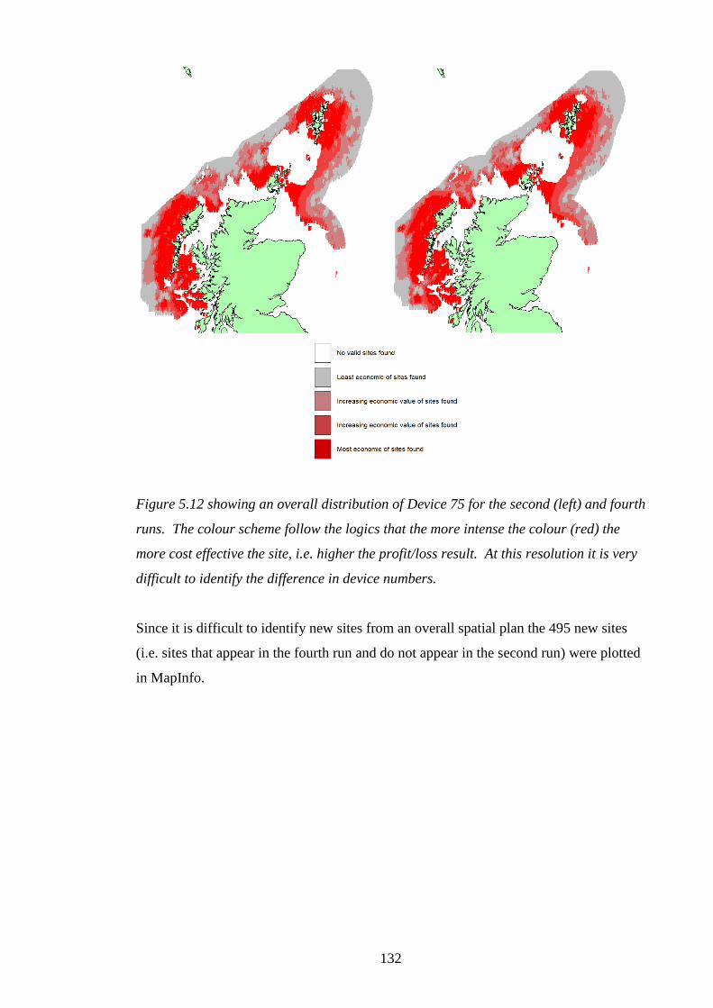
132

Figure 5.12 showing an overall distribution of Device 75 for the second (left) and fourth

runs. The colour scheme follow the logics that the more intense the colour (red) the

more cost effective the site, i.e. higher the profit/loss result. At this resolution it is very

difficult to identify the difference in device numbers.

Since it is difficult to identify new sites from an overall spatial plan the 495 new sites

(i.e. sites that appear in the fourth run and do not appear in the second run) were plotted

in MapInfo.

133

Figure 5.13 the left image shows the data difference between the second and fourth runs

for Device 75. Each point indicates an individual site. 495 sites were identified which

are all within 33kV and 132kV distance voids from various landing points. This

problem was corrected in the fourth run and therefore these sites were identified as a

result. To the right is an example for Shetland which has been focused to a level where

valid (and void) sites can be distinguished from a valid site dataset previous to the cable

data alteration.

5.5.2 Batch results, fifth run

The fifth run can be said to replicate the third, as the same data changes were made to

the devices, with the additional connection points reinstated. The methodology behind

the fourth and fifth runs is to recapture the second and third runs without the data

problem (concerning the cable distances) and therefore gain a better representation of

the valid sites. The summarised statistics from the third and fifth batch runs are shown

in Figure 5.14.

As expected in the fifth run the majority of the devices that were modified in order to

pass the test (which was also done in third run) show in the final results. There are also

a significant number of new sites found (from the previous third run) simply because

the alteration to the cable distance attributes opened up many new areas for

consideration. This is mainly with Device 75 which is the significant device in terms of

distribution due to it having a favourable attributes set.

134





Device 7 (OSPREY) 33kV 4 4

Device 7 (OSPREY) 132kV 2 2

Device 7 (OSPREY) HVDC 0 0

Device 13 (Wave Star) 33kV 115 115

Device 13 (Wave Star) 132kV 83 84

Device 13 (Wave Star) HVDC 55 55

Device 47 (TidE1) 33kV 0 0

Device 47 (TidE1) 132kV 1 1

Device 47 (TidE1) HVDC 0 0

Device 56 (Hammerfest Strøm) 33kV 0 0


Device 56 (Hammerfest Strøm) HVDC 0 0








Figure 5.14 showing the relationship between the data in the third and fifth run.

135

Figure 5.15 showing the distribution change for all devices before (third run) and after

(fifth run) the alteration to various controlling data sources. At this scale it is very

difficult to identify any difference in the two sets. Device 5 plotted in Blue, Device 75 in

Black, Device 76 in Red, Device 56 in Yellow, Device 47 in Pink, Device 7 in Grey, and

Device 13 in Brown.

As predicted in the fifth run, the number of valid sites increased. Device 75 again seen

the greatest increase with the 33kV and 132kV cable options both higher. The HVDC

option for the same device did not increased which is expected as the boundaries of the

cable distance within the database were changed for 33kV and 132kV with no change to

the boundary for the HVDC cable. Therefore, more 33kV and 132kV sites have been

found with the alteration, and the HVDC sites have been unaffected. Device 13 (Wave

Star) also had a new site identified for a 132kV cable. This was the exception to the

pattern found with the other devices, as the rest of these were not returning enough valid

sites in order for the alteration to make any difference, i.e. the parameters of these

devices were as such, that very few sites were found in the first place and the alteration

(which has only affected sites further out to sea) did not allowed any more sites to be

found.

The same data analysis methodology as before was again used on the most significant

device, Device 75, test wave device. The union results show that 32921 sites were

136

found within both the third and fifth run which is expected as this is the total of all the

cable types for Device 75 in run 3. (The fifth run expected to explicitly find new sites

and not eliminate any sites which were found during the third run analysis). This was

further confirmed when no sites were found in the data difference test between the third

and fifth runs, i.e. there were no data entries within the third run that did not appear in

the fifth run. However (and as expected) 581 sites were found in the fifth run that were

not in the third run which is a direct result of the cable attribute data change. Therefore,

the change to the model has again proved to be successful.

It is also worth noting that due to HVDC distance limit (set within the database at 500

km) there was an expectation not to find any new HVDC sites as a result of adding new

connection points.

Figure 5.16 showing an overall distribution of Device 75 for the third (left) and fifth

runs. At this resolution it is very difficult to identify the difference in device numbers, or

the distribution change of the sites per cost.

137

Since it is difficult to identify new sites from an overall spatial plan, the 581 new sites

(i.e. sites that appear in the fifth run and do not appear in the third) were plotted in

MapInfo.

Figure 5.17 showing the data difference between the fifth and third runs for Device 75.

Each point indicates an individual site. 581 sites were identified which are all within

33kV and 132kV distance voids from various landing points. This problem was

corrected for the fourth run, and therefore these sites were identified as a result.

5.5.3 Batch results, comparison between fourth and fifth runs

At this point it is also worth looking at a comparison in results between the fourth and

fifth runs, which are essentially the same as the second and third runs with the main

difference being the alteration to the cable distance values. (The second and third runs

were designed to test the change in distribution when the parameters of several devices

were changed/made more favourable, and the addition of two new connection points).

The methodology with the fourth and fifth runs comparison is the same, with the fourth

run acting as the substitute second run (with the cable distance void plugged) and the

fifth run acting as the substitute third run where the various parameters were

added/altered.

Therefore, the results from the fourth and fifth runs give a more accurate picture

compared to the previous second and third runs, where the cable distance issue became

apparent and significant anomalies in the data results were discovered. Figure 5.18

138

summarises the results for the fourth and fifth runs for the Device 75, with Figure 5.19

showing the spatial distribution for all devices in the fourth and fifth runs.





Total 33502 33502

Figure 5.18 showing the relationship between the data in the fourth and fifth run for

device 75, Test wave device.

It is worth noting that in Figure 5.18 only shows Device 75 as the other devices

(relevant to their individual runs) were unchanged and therefore have been documented

already either above or in Appendix H. In the fifth run there were also results from

devices not found in the fourth run as a result of the various alterations made to them for

the fifth run, which is not relevant for a direct comparison between the fourth and fifth

runs, and were again unchanged from the third run.

Figure 5.19 showing the distribution change for all devices before (fourth run) and

after (fifth run) the alteration to various controlling data sources. At this scale it is

difficult to identify the changes clearly, however the additional devices and sites can be

139

seen on close inspection. Device 5 plotted in Blue, Device 75 in Black, Device 76 in

Red, Device 56 in Yellow, Device 47 in Pink, Device 7 in Grey, and Device 13 in

Brown.

It is slightly unexpected that with the addition of the two landing points no additional

sites have become available for Device 75, which has the most favourable parameters

set and therefore more sensitive to changes than any other device. However, after

inspection this can be explained by the fact the new connection points allowed for a

change in the cable types within the area, rather than a change in actual sites which is

largely down to the HVDC cable having a significant range in terms of the model

boundaries.

Figure 5.20 showing an overall distribution of Device 75 for the fourth (left) and fifth

runs. The distribution change of the sites per cost can be identified with careful

inspection. In the current analysis for Device 75 the number and location of sites were

identical for both runs. The only changes appeared in the cost values in the financial

model.

140

As with the results from the second and third runs the number of HVDC sites is lower in

the fifth run than the fourth run. This is again for the same reason where the added

connection points (mainly the North Sea connection point) has allowed for the valid

sites within that area to be closer to a landing point and therefore use shorter cable

methods. The new connection points also did not allow for any new HVDC connection

due to the maximum length set for the HVDC cable (which is obviously a realistic

strength of this cable type) and the fact that the database holds a comprehensive

distribution of connection points meaning all sites in the study area are available from

the current HVDC cable setting of 500 km.

The furthest point from land according to the DTI dataset is 301.28 km and the furthest

offshore site from a connection point (fifth run) is 309.84 km. This site is located 56° 5'

2” north and 3° 15 36” east routing to Cleveland combined heat & power plant 54° 33’

22” north and 0 49’ 18” west. Incidentally this site (furthest offshore site from a

connection point) is unaffected by the additional landing points made in the fifth run.

For the study area and current list of identified landing points, a HVDC cable with its

current cable length range is a valid option for even the furthest offshore site. If in the

future the minimum HVDC distance value were less, then additional valid sites might

have been found and this could be tested by appropriately changing the cable distance

limits.

5.6 Overall summary of batch test runs

This section will provide a recap with a summary of the main batch test runs

undertaken:

First (initial) run, providing the first set of results from the model to be analysed.

Second run, after the first run it was discovered that tidal devices passed the test for

a site with significant wave regime and vice versa. The logic was altered so that the

opposing resource was considered. This alteration was then successfully tested

during the second run.

Third run, after the second run it was decided to add 2 new connection points and

favourably alter the data for 5 randomly selected devices in order to see how the

model would react. Most of the results were expected, however a data problem was

141

found in that sites positioned within the distances set for each cable type were being

ignored. The database was therefore updated to prevent this from happening.

Fourth run, after the alteration to the database following the third run, the new data

were tested within the fourth run to ensure all valid sites were found, which was

successful. Within this test the previous alterations made (to the connection points

and devices for the third run) were removed so the test acted as the second run,

without the cable data problem.

Fifth run, for completeness the fifth run was used to test the same alterations made

for the third run (addition of connection points and data alterations to the same

devices) without the cable data problem. This then allowed the distributions from

the fourth and fifth runs to be analysed with confidence that the data and logic were

working as expected.

This concludes the result documentation and testing methodology of the batch

processes.

5.7 Test comparison of batch and user facilities

As stated the user and batch modes have specific purposes. The batch mode carries out

the overall functional objectives of the model, while the user mode uses the same logic

and data, at run time, for analysis of only one specific site at a time. Therefore, the two

separate systems can actually be compared against each other to ensure they produce the

same results. This is important as one of the key strengths of the user method is to

allow (in essence) a testing facility for the user where they can see step by step how the

model has reached any particular result within the corresponding batch operation.

Although this sounds a straightforward task, i.e. considering the two methods use the

same logic and data, it still has to be tested as the actual code carrying out the logic and

interpreting the data is different due to the separate operations of the methods. The

batch mode takes every site (with every device) and works to a profit/loss result with no

interaction with the user. The user method on the other hand takes a specific site and

allows the user to select devices and conditional values and so on. Therefore, the

structure of the code (albeit with the same logic) has to be organised accordingly which

has resulted in separate methods for many of the user and batch operations.

142

Figure 5.21 showing the final profit/loss result screen for the user method at site 57.96

(57° 57’ 0”) north -7.09 (7° 5’ 0”) west (or in data location terms data row 213, data

column 100). To get to this point the user selected 200 (which is the minimum number

of devices for the HVDC cable type at this distance from landing point) Test wave

devices, which is Device 75 within the database.

Figure 5.22 Showing a data test enquiry for the same location (57.96° north, 7.09° west

/ data row 213 data column 100) for the Test wave device (Device 75) for the minimum

profit/loss result for a HVDC cable, i.e. the data inputs as for the user example above.

143

From the test example above it can be seen that the batch operation has concluded that

for site 57.96° north 7.09° west the profit/loss value is -31292012. This location within

the user operation (using the same number and type of device) confirms the overall

result value is the same. This confirms the separate code within the two separate

methods is following the design logic, and the different modes can be used to verify

each other. As a point of interest, if the overall results did not match, the data test and

user method results could have been used in conjunction as above to make a comparison

with each other in order to find out at what point the results differed. The testing

function can call up any batch output file, with any site value displayed if required.

Each stage value (i.e. each value required to eventually gain the profit/loss result) is also

displayed within the user method forms so they can be directly compared if for some

reason they did not directly correlate.

144

CHAPTER 6 – ILLUSTRATED EXAMPLE

The aim of this chapter is to show the model in use, and the true power of the dynamic

approach which this research has produced.

The example has taken inspiration from various feasibility studies undertaken for the

development of an east coast offshore grid. Of note are two studies undertaken for the

Crown Estate: East coast transmission network, technical feasibility study by Crown

Estate, Senergy Econnect and National Grid (2008), and Offshore transmission network

feasibility study by National Grid (2011).

The investigation presents an indicative set of optimum offshore and onshore electricity

transmission network reinforcements required for the connection of up to 46GW of

generation as part of the offshore wind leasing rounds (Crown Estate, 2008 / National

Grid 2011). This provides an interesting example as sections of the proposed grid

upgrade can be included in runs to see how this will change the distribution of valid

sites and their corresponding economic indictors.

The methodology will be similar to the previous test runs undertaken in Chapter 5

where model runs will take place before and after the proposed east coast grid upgrade

is added. For clarity, no hypothetical test devices were used for this illustration, and all

landing points were set to allow additional capacity to be connected.

6.1 Data to be added to include the proposed grid upgrade

The Crown Estate propose various scenarios for the east coast network linking Shetland

to north east England. The various options are not important in this context as a list of

offshore coordinates were taken to represent a sample of the Crown Estate proposals.

Figure 6.1 shows the Crown Estate indicative coordinated network design for 2030.

145

Figure 6.1 showing one of the scenarios the Crown Estate has proposed for offshore

grid development.

To relate to this example in Scottish waters, the Shetland (not shown in Figure 6.1),

Orkney, Moray Firth and Firth of Forth/Tayside offshore points were added to the

landing point dataset. This dataset already contains many east coast landing points, and

was not expanded to include onshore landing points, as the report suggests upgrading

existing landfall points, that are generally represented in the landfall dataset. The aim of

this illustration is to show a change to the offshore distribution. The offshore points are

as follows:

146

Offshore Location Latitude/Longitude DTI Water Depth

Shetland 59 53.000 -1 35.000 96 m

Orkney 58 53.000 -1 35.000 100 m

Beatrice North 58 23.889 -2 21.663 61 m

Beatrice East 58 10.000 -2 27.000 57 m

Beatrice West 58 9.000 -3 10.000 57 m

Cullen 57 48.000 -2 45.000 68 m

Tayside 56 26.000 -2 21.000 35 m

Firth of Forth 56 15.000 -1 35.000 49 m

Edinburgh 56 5.000 -2 17.000 53 m

Figure 6.2 showing the offshore points added to the landing point/connection dataset.

Figure 6.3 showing the plotted offshore connection points.

To aid the results analysis only 6 devices were used in this illustrated example. These

included 3 wave devices: Wave Dragon (Device 4), Pelamis (Device 5), PowerBuoy

(Device 26) and 3 tidal devices: Marine Current Turbines (Device 46), Hammerfest

Strøm (Device 56), Tidal Generation Limited (Device 64). From the initial testing runs,

147

some of the data entries have been updated to represent fresh information that has been

gained since the initial technological review was completed. In particular this includes:

Wave Dragon (4), minimum and maximum water depth extended, and distance to

land set.

Pelamis (5), minimum and maximum water depth extended.

PowerBuoy (26), wave and tidal regime added, distance to land and tonnage set.

Marine Current Turbines (46), minimum depth and distance to land set.

Hammerfest Strøm (56), minimum and maximum water depth set. Tidal regime

increased and distance from land set.

Tidal Generation Limited (64). Tidal regime and PTO set.

In short these alterations were expected to increase the likelihood of all 6 devices

finding suitable sites. In the previous testing at Chapter 5, only device 5 (Pelamis)

passed to a final profit/loss indication without alteration. New devices (from the

testing) have also been used for this illustration (which is not linked to the earlier

testing) to demonstrate further the operation of the model.

For this example, the HVDC cable option was also removed due to the earlier

realisation regarding the extensive distance capability of this cable in relation to the size

of the study area, that would ultimately make data analysis more difficult. If the HVDC

option were not removed, offshore sites potentially would have changed cable type,

rather than showing as a new site. This is because the HVDC cable can reach any site

in the study area from the current landing point dataset.

6.2 Model run before and after proposed grid upgrade added to database

Since the device input data has changed from the testing undertaken in Chapter 5, a

model run was undertaken before and after the additional connection points were added.

The first set of results therefore act as the benchmark for this illustrated example. The

additional connection points and subsequent model run generate two sets of results that

can be directly compared to see how the additional points change the distribution of

devices, and their economic indicators.

148

6.3 Model results and comparison of before and after model results

The results from the both model runs can be seen below in Figure 6.4

Run 6. Run 7.

Device 4 (Wave Dragon) 33kV 55 55




Device 26 (PowerBuoy) 33kV 13 13


Device 46 (Marine Current Turbines) 33kV 2 2




Device 64 (Tidal Generation) 33kV 5 5

Device 64 (Tidal Generation Limited) 132kV 0 0

Valid count 392 393

Figure 6.4 showing the relationship between the data in the sixth and seventh runs.

There is only 1 new sites identified.

As expected all devices entered returned a valid result. However, on comparison of the

two datasets it was found the results were disappointing, in that only 1 new site (in

Shetland) was found for the Pelamis device, and one site changed from a 132kV cable

to a 33kV cable as there was a closer connection point. There was also a very slight

decrease in the cost indication (3 sites lowered) from run 6 to run 7 for sites in the

region of the new Shetland offshore connection point.

On analysis of the data, it was discovered the user defined distance to land set for the

devices was a major limiting factor, that is, the offshore connection points were not

going to find new sites as the connection point distance was beyond the distance

capabilities set for the devices.

149

6.4 Further changes to input data with resulting site outputs

In order to find the true effect of the new offshore connection points, a higher figure of

70 km was set for the distance to land for all 6 devices. The model was then run again

before and after the offshore landing point additions. This change had the following

results shown in Figure 6.5.

Run 8. Run 9.











Device 64 (Tidal Generation) 33kV 5 5

Device 64 (Tidal Generation Limited) 132kV 0 0


Figure 6.5 showing the relationship between the data in the eighth and ninth runs.

As expected the model has found new sites with both Device 4 (Wave Dragon) and

Device 5 (Pelamis) as a result of the additional connection points. Pelamis had the

greatest share of the 25 new sites found.

To identify the new sites effectively, only the new results were viewed by extracted the

difference data from run 9 compared with 8, shown in Figure 6.6 below. The

connection points are also plotted with the run 9 results, to show the relationship

between the connection points and the newly found sites.

150

Figure 6.6 showing the valid results for run 8 (left in turquoise only) with entire results

for run 9 (additional new sites shown in red). On the right are the newly found sites for

run 9 only. Note the new connection points plotted in yellow.

The data analysis can be taken further to show how the connection points affected each

device.

151

Figure 6.7 showing the specific new sites found for Device 4 and Device 5 in relation to

the connection points added. Device 4 in pink, Device 5 in blue, with connection points

in yellow. Note no new sites were found in relation to the sites added around the Firth

of Forth/Tayside.

Wave Dragon and Pelamis were the only devices that were able to find new sites. The

remaining wave device (Device 26 Power Buoy) did not return any new sites as a result

of the new connection points. This can be explained by looking at the parameters sets

for the device which allowed a lower return in general. Device 26 had a 30 m depth

specified meaning only sites exactly 30 m could be considered. The offshore landing

points were all in relatively deep water (see Figure 6.2) meaning the changes had no

affect on the valid sites found.

The 3 tidal devices also did not return any new valid sites. This can mainly be

explained by the low tidal resource around the offshore connection points. If a

connection point was added in a higher tidal resource, the results would have been

different. In addition, all the offshore landing points have a relatively high wave

resource which the model does a check for, and will rule out for tidal devices.

The connection points in the south around the Tay and Forth did not allow for any new

sites as the wave and tidal resource was not adequate. This can be confirmed by

looking at the resource in the user method and by earlier testing when a hypothetical test

device with favourable attributes set also did not allow any results in this area, see

Figure 6.9.

152

Figure 6.8 showing the valid sites for the 3 tidal devices, Devices 46, 56, and 64, which

are all in the same area of the Pentland Firth. This distribution did not alter after the

addition of the new offshore connection points. Note that in 4 of the above locations

more than one device was found at the same site.

6.5 Economic distribution

There was also a very slight change in the cost distribution with an expected fall in run

9 with 2 sites showing a lower cost indication, and one other site changing from a

132kV to a 33kV site. Although a cost reduction was expected, a more marked

decrease was expected.

This is for several reasons. To explain the results, the method used to indentify the

change first has to be understood. Only sites that appeared in run 8 and run 9 can be

compared for an economic change. If we look at the east coast area in run 8 there were

very few east coast sites identified in the first place as the higher resource required was

further offshore, beyond the capabilities of device and cable. The new connection

points alleviated this problem in run 9 and new sites were found. However, since there

were few east coast sites in run 8 there were very few sites to compare economically in

run 9 as most of the east coast sites were new. The sites that did show a reduction are

shown in Figure 6.10.

56, 64

56, 64

56, 64

64

56, 64

46

46

153

This reasoning can further be confirmed by looking at the previous forth and fifth runs

where a hypothetical wave device (Device 75) had favourable parameters set which did

allow for offshore east coast sites. An addition of an offshore connection point (in the

Moray Firth area of the North Sea shown in Figure 6.10 as the most easterly yellow

plot) did allow for a significant economic change in distribution for this area, as there

were available sites for comparison in both run 4 and 5. Figure 6.9 shows the

distribution for Device 75 during these previous runs.

Figure 6.9 showing an overall distribution of Device 75 for the fourth (left) and fifth

runs. Note the lack of sites found in the south east for this hypothetical device set with

favourable parameter data.

154

Figure 6.10 showing the 2 sites in Shetland (blue) that experienced a lower profit loss

result as a result of the new connection points which are shown in yellow and black.

The other yellow plot is the offshore connection point added in run 5 that allowed a

significant reduction in cost with the hypothetical device which had a favourable water

depth and distance to land set to allow offshore sites to be found.

There are other important economic considerations with the addition of offshore

connection points. Although a connection point will become available with a low cable

cost (due to decreased distance) the water depth is likely to be higher for new sites, and

distance to port further so the installation/decommissioning costs will rise. Many of the

values in the database are mainly test values or values gained from other industries

which may not show the true trade-off between such changes, i.e. fully understanding

the scale between the various cost sets in the database. Therefore newly found offshore

sites will be higher even with the new connection points, when compared to sites closer

to shore with a similar distance to a connection point.

As the illustrated example did not check the load capacity availability of onshore

connection points (which will be an important consideration as most onshore connection

points are likely to be running at capacity) the true distribution of the newly added

connection points was not shown. This is considering the model checks for the closest

landing point which will likely have no capacity available, these values were artificially

set to allow the model to proceed. Therefore, the new offshore connection points may

have been the closest point with spare capacity. To carry out this logical test the

landing points without spare capacity can be reset to reflect the actual capacity.

Removing landing/connection points without capacity from dataset would also have the

same effect. This action would have a marked effect on the sites found, with Shetland

site for example likely not to appear due to the lack of spare capacity.

6.6 Overall findings

From the illustrative example undertaken there are several key points that can be made:

Changes made to the device dataset (with new information) had a positive affect in

that each device returned valid sites. This can be seen further when comparing the

155

testing undertaken in Chapter 5 where Pelamis (in smaller numbers) was the only

device to have returned a valid site.

The various model logic worked as expected. The distance to land test for example

prevented new sites being found even when offshore landing points were added.

The addition of the offshore landing points had a positive result for devices that

would allow this change, in terms of the device having suitable attributes such as

distance to land. This allowed sites to be found further offshore.

With the addition of the offshore landing points (in this illustration and previous

run 5 example) the economic distribution of the valid sites has changed, lowering

the cost for site development.

156

CHAPTER 7 – HOW THE MODEL COULD BE IMPROVED

Although a working model has been produced, it does not claim to be complete. The

ideal model was presented in Chapter 3, however this was impractical to build mainly

because of time and available data. From the ideal design a working model was

produced and one that can be readily extended in order to get closer to the ideal model.

This chapter describes in detail how the model could be improved, and is structured to

reflect the sequence of steps undertaken:

A list and recap of the missing constraints and functionality omitted from the as

built model from the ideal model design, (7.1)

Improvements that could be made to the data and program resolution, (7.2).

A full description of the further functionality (over and above originally

designed for the ideal model) that can be added such as: logical detail, data

addition, result data management, human computer interaction, economic

features, cabling modelling, pipeline and shore station modelling, hydrodynamic

modelling, automated automisation, and automated data formatting. (7.3)

Feedback and possible future usage of the model (7.4).

7.1 Missing constraints and functionality

The as built model is only a working representation of the ideal design and omits some

of the constraints analysis and functionality. The elements that were removed to

construct the working example of the model are essentially detail, as the main structure

stayed in pace with, albeit at a much higher level. As a recap, the idealised list of

datasets identified to construct the ideal model was as follows:

Resource data such as wave, tidal, and wind.

Bathymetry.

Other physical data such as geological data to confirm the condition of the seabed

and so on.

Areas of high vessel density associated with narrow channels and shipping.

157

Offshore structures such as in the oil and gas industries and their associated

pipelines, safety zones and so on.

Offshore electrical and telecommunication cables.

Wrecks and other marine archaeological sites.

Former dumping grounds and contaminated areas.

Military zones such as training areas and bombing ranges.

International shipping lanes and areas of high vessel density.

Fishing grounds and aquaculture.

Offshore wind (various deployments and leasing rounds), and of course other MEC

developments.

Other activity areas and licencing.

Other marine resource extraction such as marine aggregate dredging.

Areas of high recreational use.

Protected and special sites, such as: Special Protection Area (SPA), Sites of Special

Scientific Interest (SSSI), and Special Areas of Conservation (SAC), National

scenic areas, RAMSAR (Convention on wetlands) sites, Marine Nature Reserves

(MNR), National and Local Nature Reserves (NNR/LNR).

Areas close to protected sites where the designation includes mobile species such as

seals and birds.

Other environmentally valuable sites (that are not officially designated), such as:

maerl beds, reefs and so on.

Breeding areas for: birds, seals, cetaceans and fish such as herring spawning areas

For the working model bathymetry, resource data (wave and tide) and distance to land

were essential features to include. These allowed the basics of a model to be built as

these are constraints that can technically prevent a development. The other constraints

may not prevent a development, but rather create a problem that will be different for

each device.

However for an accurate development appraisal to take place, many site constraints (the

development risks) will need to be known. These constraints will determine the likely

route through the planning and consents process, as well as give an indication of any

device redesign (such as moorings for example) and any additional costs.

158

The way in which the model would handle these additional datasets is essentially the

same as the constraint methods already in place. For the constraints that would not stop

the development from a technical point of view, the model would not rule out that site

as it does with the current physical constraints. Rather, the model would show that a

constraint exists and determine through logic (using methods to compare the device

datasets against constraints) the increased risk. Obviously if many constraints exist, the

overall development cost will increase proportionately. Each constraint will pose a

different risk to a particular device and it is only a matter of adding in the additional

constraints data and any particular logic to test the particular constraint against a device.

An example here would be to compare a device mooring with the geology at a particular

site.

The economic appraisal and cabling methods of the working example were scaled back

significantly form the original ideal design. This is mainly in terms of detail, where

levels of additional costs (maintenance, finance etc) and revenue (ROCs and other

financial incentives) calculations were only carried out at a high level. The original

ideal design would allow for more accurate cost and revenue values such as adding

discounts rates for Discounted Cash Flow (DCF) to give a Net Present Value (NPV) of

the project. The Internal Rate of Return (IRR) could also be generated at this point,

which in turn would improve the accuracy of the overall profit/loss indication. Thus it

would be beneficial for these original designs to be implemented, but this in time will

depend on more data being available for each device.

The original model was also conceived with a hydrodynamic function. This was to

determine the most efficient packing density of an array development by calculating

energy losses and turbulent effects of an array. A fuller discussion on packing density

is detailed at: A.8 Calculate the number of devices required and device output at a given

site.

The hydrodynamic function would allow a more dynamic look at surrounding sites to be

added so that cable requirements (in particular minimum output from a device array)

does not force high packing densities on a particular site, as presently experienced with

the working example. Therefore a single site may actually turn into several sites to fit

the number of devices required to satisfy the cable specification. The design

specification of the hydrodynamic model (and sequence within the ideal model) is

159

discussed in 3.5.1 Finding a valid site. Alternatively the model could handle

hydrodynamic data as inputs which is discussed at 7.3 Further functionality.

Many of the self constructed datasets were setup with future modifications in mind,

with many datasets containing additional data that is not processed by any logic, such as

additional device statistics and parameters. Some of these were setup before the

decision was made not to undertake the ideal model but are available for future use.

7.2 Data and program resolution

The data included in the working model has been proven to be at a resolution much too

coarse to provide adequate results, particularly inshore sites and areas with narrow tidal

channels. This was a downfall partly of modelling an area the size of Scotland and her

seas, and partly of the resolution of the available data.

An improvement would be data at a finer resolution. The model design allows smaller

areas (such as the Pentland Firth where the volume of fine resolution data are

increasing) to be added without any redesign of the model structure or code. The model

could work at various resolutions, providing say a regional and nested localised view

where data exists. Either the regional model could be run in order to find areas of

interest which could be studied in more detail with finer datasets, or the model could

run to the resolution of the finest dataset. The latter could be implemented by either

converting all datasets to the finest dataset before processing by the model, or by the

model checking the resolution of each dataset and reading the closest value (or by using

methods such as interpolation or kriging) at any given location for datasets at a lower

resolution. This would allow datasets of various resolutions to be processed at the same

time.

7.3 Further functionality

There is simply not room to discuss all possible additional features and functionality,

however some of these are considered further below.

160

7.3.1 Logical detail

There can be many improvements made to the functionality the code provides. One

such example, as already shown, was the improvement made to the logic after the first

initial run of results. The resource methods were modified so that the logic discarded

any significant wave sites with large tidal resource and vice versa. This is an example

of significant improvement to the logical function of the model which was done with an

insignificant alteration to the code. This is the sort of logical detail (programming

tasks) can be extended within the data structures that already exist. This example can be

taken further as it would be a beneficial addition if the opposition tidal/wave resource

could be controllable i.e. a switch option to turn on or off, and increase or decrease the

tolerance value so the differences can then be analysed. This in turn would depend on a

better understanding of how wave and tidal current interactions affect each device.

There are many other improvements that can be considered, such as improving the logic

used for distances between points in the model.

7.3.2 Data addition

Within the working model there are a lot of record entries that are not complete. Device

datasets is a good example of this, as many of the key factors of a device have to be

known in order to allow the model to proceed. The more complete the valid data used,

the more accurate the final result. In the case of devices, many identified devices are

not considered by the model as key features are not known. If they were known, the

results are likely to have been different as shown in earlier testing (Chapter 5) by

experimenting with altering (and adding) input values for devices.

Since the various model test runs were undertaken for this thesis, there has been the

release of several new devices. The industry is moving extremely fast at present, and

there are new designs from existing and new companies emerging on a regular basis. It

would therefore be beneficial to keep the device datasets up to date and run the new data

through the model as soon as it is obtained.

161

7.3.3 Result data management

The model, as described, has a results function where the valid results can be displayed

in various lists. However, without various computing (and in particular database and

GIS skills) then the results at present are not easy to visualise. It is quick and easy to

discover the best site for a device and cable and so on, however, to actually change one

data field within the database and see how this affects the distribution is not so easy.

This is only possible at present by working with data outputs with other tools such as

GIS. However, an in built GIS display system would make this sort of result viewing

much easier. This would be more beneficial than using database queries and program

scripts for example to find the differences in result datasets, which ideally need to be

plotted into other tools. This consideration is particularly important if the model is to be

developed and used by an end user that may not necessarily have GIS, database or other

general programming skills. To keep with the open source theme of the project, an

automated Google Earth/Maps output would be priority during this work.

7.3.4 Human Computer Interaction (HCI) considerations

From a user point of view improvements could be made to make the entire application

more user friendly. This applies to use of the underlying database, right through to

analysing the final results.

The database that is used to store many of the datasets the model uses, is at a basic level

in Human Computer Interaction (HCI) terms. There is no Graphical User Interface

(GUI) associated with any of the base datasets which makes appending or editing data

slightly more problematic if the user was unfamiliar with database record sets.

Therefore, standard Windows GUI tools and functions would make viewing, appending

and editing data in the database more straightforward.

The same argument applies here to the various inputs and outputs the model is working

with. The current setup is to process one collection of data at one time, which has to be

predefined in the database. The model can only process one collection of data at a time,

outputting one set of collection output files from predefined input data. The current

procedure to switch between the input and output data locations is logical in terms of a

162

user with computing/programming skills. However, the model will over a period of

time ideally work with multiple data collections, that is, provide a GUI selectable option

for the user to load for input, and where to save the output files. This would eliminate

the need to change any database or code entries, and the names of files and directories.

The model output files could also be formatted automatically to other software

standards such as MapInfo, Google Earth and so on. This would allow the results to be

loaded and viewed more easily.

7.3.5 Economic features

Over and above the ideal design there are several additional economic features that can

be added. One such example could be the addition some economic controllers, where

scales and thresholds can be set, such as for a project budget. This could take the form

of another filter in the overall equation that could be also be used to turn on or off

spatial results, if profit/loss over (or under) budget, or specified internal rate of return.

There are many more additional economic features, techniques and methodologies that

could be used to expand the economic functionality of the model. Another such as

example would be to include economy of scales for a MEC development.

7.3.6 Cable modelling

The current cabling method could be expanded to include additional functionality and

therefore a more robust cable selection method. There are many considerations such as:

Cable configurations. This is a new and developing technology for the marine

energy sector and MEC cable methods cannot be realistically compared to other

cable projects, other than offshore wind at present. Information from the wind

industry is hard to establish, as each project is unique. There can also be added

logical detail to include various configurations for the same site, the as built model

only considers one ideal cable configuration determined by cable distance.

However, it would be valuable to compare various different configurations at the

same site.

163

Routing algorithms, the site to shore will not be a straight route as assumed at

present, and therefore all distances will most certainly be longer. Additional

algorithms will also be required to work out the cable length (and therefore cost) to

link up each device within the array. There will also be the need to look at the

cable route in terms of constraints (physical and non physical) that may prevent a

cable deployment, or increase the cost. This can be achieved by comparing the site

constraints against the cable in the same way the model compares the site

constraints against a device.

Cables may need to be buried/spanned/armoured in various areas.

Specific devices will require specific solutions, affecting installation costs.

Grid tariffs, such as firm and non firm grid connections and connection charges.

Additional onshore requirements such as routing, available capacity throughout the

network etc.

To include this level of detail, a separate project or sub model could be incorporated

into the overall logic of this project on completion. This is consistent with the overall

design, as the overarching model basically sits on top of many sub models (functions)

that all have specific tasks. A sophisticated cable model could be developed

independently and brought into the overall model to work with the other existing sub

models.

7.3.7 Pipeline and shore station modelling

Since not all the devices convert extracted energy to electricity offshore, there will be

need to cater for devices such as the Oyster that uses an offshore pumping system to

drives an onshore hydroelectric system. For this category of device, a pipeline model

would be used instead of an offshore cabling model, which share a similar

methodologies, such as distance, device capacity, route, price per km and so on. A

further method could also be added to locate suitable sites for onshore conversion

stations. This will be an important consideration to identify these terrestrial locations,

as well as having a bearing on many other variables such as the offshore distance

calculations.

164

7.3.8 Hydrodynamic modelling

Another benefit to the model would be the inclusion of a hydrodynamic model as

discussed previously. However as hydrodynamic models are a very specific product, it

may be beneficial to use hydrodynamic data as an data input much in the same way as

the cable sub model.

The main overall advantages of including a hydrodynamic model are discussed at 7.1

Missing constraints and functionality. Providing a robust hydrodynamic model would

allow a great deal of additional functionality to be developed, such examples include:

Predictions of actual wave and tidal resource at any particular site, including tidal

cycle.

From the above example, if we consider the tidal resource in more detail and in

particular the resource through the water column. The velocity will vary

significantly from the surface to the seabed, which is understandably difficult to

model considering each site is likely to be different. The DTI data tidal power is

calculated for the upper (50%) of the water column.

Selection of tidal devices, as well as where they could be placed. Following on

from the resource through the water column modelling, ideal rotor dimensions at

any given location can be determined. The converse is also true as the model

could answer the question: how significantly would a particular device need

tailored for a particular site?

7.3.9 Automated automisation

The model could also be automated with the inputs required to find favourable results

determined iteratively by code that is integrated in the application. This would work

along the lines of running the current batch program, and when results for devices and

sites do not pass, then the model could review and record the critical values as a form of

sensitivity analysis. The model could loop around to test the critical values again

which would ultimately give a set of values (in separate data output files) that a device

would have to possess if it were to produce a valid profit/loss indication.

165

The output would be a significant volume of files which would have to be analysed in

an automated fashion, giving more work to the result data management function of the

model.

7.3.10 Automated data formatting

It would also be beneficial to construct a software tool to automate further the data

formatting processes. With any programme logic, there is a desired format for input

data, so the task would be to set up a tool to format any kind of data to the input

specification. This would require a significant amount of code and logic, however it

would allow more external datasets to be quickly converted for the model to use. A

software tool of this kind would also have the functionality to turn non formatted spatial

data into such for the model’s benefit. The integrated tool would be used to convert

data into the model format before future modelling, and therefore not need to be

undertaken within each model run.

7.4 Feedback and possible further usage

At this point in development, it would also be beneficial to take the work produced to

industry for feedback, i.e. what would a developer or planner like the model to do, and

what would they see as a logical development path.

In general it would also make sense for the model to be used from a user/planner point

of view rather than a software developer point of view, to find out exactly what it can

show us. The model has been developed to carry out a specific set of logical tests and

some of the results have been analysed, however, it has not been trialled by others to

any great extent. Therefore, it would be beneficial for the model to be used over a

period of time, putting it to the task it was designed for (indicating where MECs can be

deployed). It is also more than likely that different users would wish to tailor the model

to a specific purpose, depending on their particular priorities.

With model structure in place, there is potential to add functionality and additional data

to analyse shoreline devices. This is also true of other forms of technology such as

offshore wind as the methodology is transferable. The model could also be set up to

produce dataset layers to aid zoning and therefore act as inputs to a conventional marine

166

spatial planning tool. It could also be set up to address onshore spatial planning

questions within the terrestrial environment.

167

CHAPTER 8–DISCUSSION AND CONCLUSION

One of the main stated aims of this research was to produce a site appraisal model that

could provide a more dynamic and efficient approach than currently available through

convention Marine Spatial Planning (MSP) approaches. MSP, through techniques such

as constraint zoning, unnecessarily rule out no go zones, which could be more

effectively treated as developers risk, even in protected areas. As a result of zoning

“free space” is identified which may be inappropriate for MEC development as various

criteria (such as resource) may not exist in this free space. A model was necessary to

show the valuable sites to MEC development, highlighting where the pressure would be

to develop with the available resource, grid, technology and so on.

An idealised predictive model was designed to achieve this aim. However due to time

constraints and lack of data for the overall study area this design was not feasible. A

working model was produced with a framework that can be expanded to encapsulate all

aspects of a fully functional model. The data and functionality omitted from the full

model design can in most parts be easily be assimilated to the working model and

therefore can be upgraded in stages. There are new and improved datasets available at

present (and continue to become available) that there was not time to include. This is

also true of functionality such as the various economic calculations that can also be

added with ease, although unknown aspects such as maintenance and weather window

are likely to remain problematic. It was acknowledged early in the project that the ideal

model could not be built, however it was important to design the model in its ideal

form, and produce an overall scaled version rather than concentrating on smaller

aspects. Therefore, a working example was successfully constructed to demonstrate and

confirm the overall methodology.

Although the model produced is only a working representation, the functionally

included has shown to be extremely flexible and powerful. The construction of the

application is such that technologies, cables, landing points, ports and so on can be

added, amended and deleted with ease, meaning this tool can interact with a significant

number of variables with no intervention from the user once set to run. This allows the

model to be run with varying input data very effectively, and has shown to have a

significant affect on the output results. This dynamic approach allows any stored value

to be changed, which depending on the value’s significance will have an affect on the

168

overall physical site and economic distribution. This was highlighted in the various

testing and illustrated examples where several small changes to device parameters, and

the inclusion of new landing points had a significant change in the resulting

distributions.

The resulting tool, although designed to be used for developers and investors, provides

improved information to the planners than resource maps do at present. Additionally it

is able to provide information if circumstances change in terms of grid capacity, cabling

and technology which will be of significant benefit to the industry. For example a

technological neutral company can use the model to determine which method would

best suit a site. The industry is in an early uncertain stage with no clear indication of

which technology (in terms of MEC, cabling, grid solutions and so on) is best suited to

the emerging marine energy problem, so a dynamic tool is required to give an indication

of what the best technology is to use. This is an important feature as this development

appraisal approach allows easy identification of potential commercial sites which has

not been possible before now.

The research has made a number of recommendations for future development with

attention to detail, and more accurate and comprehensive data being the key identified

issues. Ideally, the working example should be extended to incorporate the full design.

There are also various recommendations to improve the overall model even further with

a continued resource. Many development proposals have been documented, only

possible due to the foundation laid by the construction of the working model. The level

of detail and inclusion of additional datasets can be a continual process as knowledge is

gained. There is also the potential to improve the use of the model application and how

the results are analysed and presented, which at present is not as user friendly as it could

be.

Another key feature of the application model is that it has been developed in various

tools all of which are inexpensive to buy. There is an argument that the modelling

could have been undertaken in other packages such as IDRISI or ArcGIS, however, it

was felt extremely important to keep the work as open source as possible, with the

added advantage Microsoft windows products allowing enhanced usability through the

various graphical tools that can be used. An executable application file is provided with

this thesis which does not need a Visual Basic (VB) compiler to run. If the model is to

169

be altered the VB development software will be required. However, Microsoft VB and

Access (part of the Office suite) are both inexpensive off the shelf products that can be

used to develop or amend the model. The full code listings are also available and the

code for the batch mode has been documented in pseudo code so that the model can be

coded in any programming language. Therefore, the methods and calculations of the

model are not only open source, but fully transparent.

Therefore, a powerful tool has been produced that can be used and developed

inexpensively. It can also be developed further with off the shelf products or in a new

development environment with the documentation provided in this thesis.

This will allow the end user to model various scenarios in a dynamic and flexible way,

showing the true power of the model. Although test and demonstration examples have

been documented, the true value of this thesis will be shown in the use of the model to

help answer complex problems. The model has the potential for much more advanced

and powerful operation in addition to its current capabilities, which can be summarised

as:

A more advanced tool for developers, planners and investors using a specific form

or technology, or finding a technology for a specific site.

A beneficial use for organisations such as the Crown Estate and Marine Scotland

in identifying with spatial planning economically efficient use of the resource.

More advanced modelling functionality that is not instantly obvious from the

already established design functions above. One such example would be to

further understand the conclusions drawn from the recent Ofgem significant code

review, which sets out new transmission charging arrangements. Within this

report Ofgem reiterates its argument that generators should pay for the costs

which they impose on the transmission network, which will inevitably increase

project costs on islands (Ofgem, 2012, 2).

There are mitigating principles that have been suggested, such as generic/average

cable costs used for islands rather than actual costs to ensure consistency,

extension to the Active Network Management (ANM) scheme with charges based

on usage rather than installed capacity, re-examining island security factors, and

the treatment of expensive HVDC convertor station costs. In short, these can be

170

considered as complex economic proposals, and their consequences are difficult

to quantify without the help of modelling to determine the economic distribution

change of such measures.

The model developed in this thesis can be setup to show the economic distribution

for each solution (with the economic scenarios catered for by refining the added

project costs) and various combinations of these. Various model runs with each

scenario would be undertaken to allow a picture of what solutions would work

best for a particular area, i.e. show the distribution change with the distributed

project costs. The results may show that another solution may be needed for

island projects to be economically feasible, such as the idea of island ROCs.

Alternatively, the results may show the current system in place will allow some

island projects to be feasible as Ofgem are suggesting, or a situation that will stifle

growth as feared by industry (Baster, 2012). This is just one example of how the

model can be used as economic situations arise. The connection charge issue

above is a complex situation that is causing deep concern (Scottish Renewables et

al., 2012) with, until now, no easy way to answer such questions.

Another further modelling example would be to analyse optimal cable connection

points. The model could be set up to run in multiple time to determine where the

best cable connection points would be in terms of the resource, and also the

capacity these would need for different scenarios of development. This would

work by running the model from the start to end location geographically to

determine the project costs at each location with a new connection point added.

Once each location has been calculated, a comparison can be made to test where

would be the most economically feasible locations for connection points. Similar

tests would also be carried out to indicate the most feasible landfall points,

additional landfall points, and landing points to upgrade. There is also the

potential for the model to produce random data for many of the unknown inputs.

This would allow the integration of Monte Carlo experimentation with the model

data.

The above multiple time functionality, in conjunction with a hydrodynamic

modelling element, would also help define the device on device impacts where the

resource at each site can be modified considering neighbouring developments.

171

Therefore, the technique and methodology provided in this research is able to provide

the marine renewable industry with a unique site appraisal tool. This will assist

technological developers, who can spend their limited time and resource on their

devices, rather than trying to identify sites to deploy them. Effective and planned MEC

deployment will ultimately help the emerging marine renewable industry achieve

commercial energy extraction, and assist Scotland in realising her renewable energy

potential.

172

REFERENCES

Aegir Wave Power (2012). The Shetland Project. Available:

http://www.aegirwave.com/the-shetland-project.aspx. Last accessed 11/07/2012.

Ames, A.L., Nadeau, D.R. and Moreland, J.L. (1997). The VRML 2.0 Sourcebook.

New York: Wiley.

Aquamarine Power (2012). Technology: How Oyster wave power works. Available:

http://www.aquamarinepower.com/technology/how-oyster-wave-power-works/.

Last accessed 11/07/2012.

Akwensivie, F., Chandra, P., McAlister, C., Murray R., Sullivan, N. (2004). Marine

Current Energy Baseload Supply Strategy for Scotland. Strathclyde University.

Available: http://www.esru.strath.ac.uk/EandE/Web_sites/03-

04/marine/index2.htm. Last accessed: 12/07/2012.

Bahaj A.S., Myers L.E., Thomson M.D. and Jorge N. (2007). Characterising the

wake of horizontal axis marine current turbines. Proceedings Seventh European

Wave and Tidal Energy Conference, Porto, Portugal.

Baster, J. (2012). OIC Briefing, Ofgem’s Significant Code Review Conclusions.

Orkney Islands Council (unpublished paper).

British Wind Energy Association (BWEA) (2006). Path to Power Wave and Tidal

Stream Energy around the United Kingdom Legal and Regulatory Requirements.

Available: http://www.bwea.com/pdf/pathtopower/Stage1.pdf. Last accessed

10/07/2012.

Brooke, J. (2003). Wave Energy Conversion Handbook. Oxford: Elsevier Science.

Bullen, C.R. and Dacre, S. (2002). Pentland Firth Tidal Current Energy Feasibility

Study - Phase 1. Available:

http://www.see.ed.ac.uk/~ibryden1/REE/Tidal%20Power%202008/Pentland%20

Firth%20Feasibility%20Study-%20phase%201.pdf. Last accessed 10/07/2012.

Bryden, I.G., Bullen, C.R., Baine, M.S. and Paish, O. (1995). An Assessment of

Tidal Streams as Energy Sources in Orkney and Shetland. Underwater

Technology: The International Journal of the Society for Underwater, Volume

21/Number 2, 21-29.

Cameron, D. (2010) Prime Ministers Speech at DECC. British Prime Minister’s

Office. Available: http://www.number10.gov.uk/news/pms-speech-at-decc/ Last

accessed 11/07/2012

173

Carbon Trust (2011). UK tidal current resource and economics study. Available:

http://www.carbontrust.com/media/77264/ctc799_uk_tidal_current_resource_an

d_economics.pdf. Last accessed 11/07/2012.

Crown Estate, National Grid, and Senergy Econnect (2008). Round 3 Offshore

Wind Farm Connection Study. Available:

http://www.thecrownestate.co.uk/media/214346/round3_connection_study.pdf .


Department for Business, Enterprise and Regulatory Reform (BERR) (2008).

Renewable Atlas Technical Report and associated data. Available:

http://www.renewables-

atlas.info/downloads/documents/R1432_Final_15May08.pdf. Last accessed

10/07/2012.

Department for Business, Enterprise and Regulatory Reform (BERR) (2008).

Renewable Atlas. Available: http://www.renewables-

atlas.info/downloads/documents/Renewable_Atlas_Pages_A4_April08.pdf.


Department of Energy and Climate Change (DECC) (2003). Offshore Wind Farm

Development Strategic Environmental Assessment. Available:

https://www.gov.uk/government/publications/offshore-wind-farm-development-

strategic-environmental-assessment-r2-wind-environmental-report. Last

accessed 10/07/2012.

Department of Energy and Climate Change (DECC) (2003). Energy White Paper

Our energy future – creating a low carbon economy. Available:

http://webarchive.nationalarchives.gov.uk/+/http://www.berr.gov.uk/files/file10

719.pdf. Last accessed 10/07/2012.

Department of Energy and Climate Change (2009). The UK Renewable Energy

Strategy. Available: http://www.official-

documents.gov.uk/document/cm76/7686/7686.pdf. Last accessed 10/07/2012.

Department of Energy and Climate Change (DECC) (2010). Severn Tidal Power,

Feasibility Study Conclusions and Summery report. Available:

http://www.decc.gov.uk/assets/decc/what%20we%20do/uk%20energy%20suppl

y/energy%20mix/renewable%20energy/severn-tp/621-severn-tidal-power-

feasibility-study-conclusions-a.pdf. Last accessed 10/07/2012.

Department of Energy and Climate Change (DECC) (2011). Offshore energy

Strategic Environmental Assessments. Available:

174

https://www.gov.uk/government/organisations/department-of-energy-climate-

change/series/offshore-energy-strategic-environmental-assessments. Last


Department of Energy and Climate Change (DECC) (2011). Chapter 5 of the

Digest of United Kingdom energy statistics (DUKES) for 2011. Available:

http://webarchive.nationalarchives.gov.uk/20121217150421/http://www.decc.go

v.uk/assets/decc/11/stats/publications/dukes/2307-dukes-2011-chapter-5-

electricity.pdf. Last accessed 10/07/2012.

Department for Environment, Food and Rural Affairs (Defra) (2004). The Irish

Sea Pilot. Available: http://jncc.defra.gov.uk/pdf/irishseapilot_all.pdf. Last


Department for Environment, Food and Rural Affairs (Defra) (2006). Marine

Spatial Planning Pilot, Final Report. Available:

http://www.abpmer.net/mspp/docs/finals/MSPFinal_report.pdf. Last accessed

10/07/2012.

Department of Trade and Industry (DTI) (2004). Renewable Atlas Data and GIS

Systems used, published on CD ROM.

Department of Trade and Industry (DTI) (2007). A White Paper on Energy.

Available:

http://www.decc.gov.uk/assets/decc/publications/white_paper_07/file39387.pdf.

Last accessed 11/07/2012

Duxbury and Duxbury (1993). Fundamentals of Oceanography. USA: Brown

(William C.) Co.

Electricity Networks Strategy Group (ENSG) (2009). Our Electricity Transmission

Network: A Vision for 2020. Available:

http://webarchive.nationalarchives.gov.uk/20100919181607/http:/www.ensg.go

v.uk/assets/1696-01-ensg_vision2020.pdf. Last accessed 10/07/2012.

Electric Power Research Institute (EPRI) (2011). Mapping and assessment of the

United States Ocean Wave Energy Resource, Technical Report. Available:

www1.eere.energy.gov/water/pdfs/mappingandassessment.pdf. Last accessed

10/07/2012.

EPSRC/Edinburgh University (2007) Supergen Marine Energy Research Full Report.

Available: http://www.supergen-

marine.org.uk/drupal/files/reports/supergen_2007_monograph.pdf. Last


175

European Commission (1996). The exploitation of tidal marine currents (non-nuclear

energy JOULE II project results. Report EUR 16683EN. Luxembourg : DG

Science, Research and Development. European Commission Publishing.

European Commission (2008). Roadmap for Maritime Spatial Planning: Achieving

Common Principles in the EU /* COM/2008/0791 final */. Available: http://eur-

lex.europa.eu/LexUriServ/LexUriServ.do?uri=COM:2008:0791:FIN:EN:HTML


European Commission (2010). Maritime Spatial Planning in the EU - achievements

and future development /* COM/2010/0771 final */. Available: http://eur-

lex.europa.eu/LexUriServ/LexUriServ.do?uri=COM:2010:0771:FIN:EN:HTML


European Marine Energy Centre (EMEC) (2009). Assessment of tidal energy

resource. Available:

http://www.emec.org.uk/download/4%20Assessment%20of%20Tidal%20Energ

y%20Resource.pdf. Last accessed 10/07/2012.

European Marine Energy Centre (EMEC) (2011). About us. Available:

http://www.emec.org.uk/about-us/. Last accessed 10/07/2012.

European Marine Energy Centre (EMEC) (2011). Scale site clients. Available:

http://www.emec.org.uk/about-us/scale-site-clients/ Last accessed 10/07/2012.

European Marine Energy Centre (EMEC) (2012). Various wave and tidal clients.

Available:

http://www.emec.org.uk/about-us/our-tidal-clients/voith-hydro/

http://www.emec.org.uk/about-us/wave-clients/wello-oy/

http://www.emec.org.uk/about-us/our-tidal-clients/scotrenewables/

http://www.emec.org.uk/about-us/our-tidal-clients/andritz-hydro-hammerfest/

http://www.emec.org.uk/about-us/our-tidal-clients/atlantis-resources-

corporation-2/

http://www.emec.org.uk/about-us/wave-clients/eon-uk/

http://www.emec.org.uk/about-us/wave-clients/scottishpower-renewables/

http://www.emec.org.uk/about-us/our-tidal-clients/open-hydro/

http://www.emec.org.uk/about-us/wave-clients/aquamarine-power/


European Marine Energy Centre (EMEC) (2012). Wave test site. Available:

http://www.emec.org.uk/facilities/wave-test-site/


176

European Wind Energy Association (EWEA) (2009). Wind at work, wind energy

and job creation in the EU. Available:

http://www.ewea.org/fileadmin/ewea_documents/documents/publications/Wind

_at_work_FINAL.pdf. Last accessed 10/07/2012.

Faber Maunsell/Metoc (2007). Scottish Marine Renewables SEA, Environmental

report. Scottish Executive. Available:

http://www.scotland.gov.uk/Resource/Doc/1086/0048531.pdf. Last accessed

11/07/2012.

Forum for Renewable Energy Development in Scotland (FREDS) (2005).

Scotland’s Renewable Energy Potential: realising the 2020 target. Available:

http://www.scotland.gov.uk/Publications/2005/09/09144010/40120. Last


Forum for Renewable Energy Development in Scotland (FREDS) (2009). Marine

Energy Group’s (MEG) Marine Road Map. Available:


10/07/2012.

General Bathymetric Chart of the Oceans (GEBCO ) (2003). One Minute Grid

Data – a global one arc-minute grid, updated 2008. Available:

http://www.gebco.net/data_and_products/gridded_bathymetry_data/ Last


Glynn, J., Hamilton, K., McCombes, T., MacDonald, M. (2006). Marine Current

Resource and Technology Methodology. Strathclyde University. Available:

http://www.esru.strath.ac.uk/EandE/Web_sites/05-

06/marine_renewables/home/welcome.htm. Last accessed: 12/07/2012.

Hammonds, T.J. (1993). Tidal Power. Institute of Electrical and Electronics

Engineers, 81, 419 – 433.

HM Revenue & Customs (2011) Climate Change Levy. Available:

http://www.hmrc.gov.uk/climate-change-levy/index.htm. Last accessed

10/07/2012.

HMSO (1981). Tidal power from the Severn Estuary, Volume 1: Energy Paper 46.

HMSO (1989). The Severn Barrage Project: General Report. Energy Paper 57.

ICIT and European Union (1995). Feasibility Study of Tidal Current Power

Generation Power Generation for Coastal Waters: Orkney and Shetland, Final

Report. EU contract XVII=4 1040=92-41. Heriot-Watt University.

177

IronsideFarrar (2010). Strategic Environmental Assessment, Environmental Report, A

Marine Spatial Plan for the Shetland Islands. Available:

www.nafc.ac.uk/.../Files/Part%20One%20Policy%20Framework.pdf. Last

accessed 10/07/2012

Korea Herald (The) (2010). Garolim and Incheon tidal barrage projects. The Korea

Herald Available:

www.koreaherald.com/specialreport/Detail.jsp?newsMLId=20090727000092.


Lee, Kwang-Soo. (2006). Coastal Engineering Research Department, Korea Ocean

Research and Development Institute, Tidal and Tidal Current Power Study in

Korea. Presentation. Available:

http://www.docstoc.com/docs/46343368/Tidal-Current-Power-Development-in-

Korea. Last accessed 10/07/2012

Marine Scotland (2010). Sustainable Marine Environment Initiative, Project

Evaluation. Available:

www.scotland.gov.uk/Resource/Doc/295194/0100906.doc. Last accessed

10/07/2012

Mather, J. (2010). Scottish Government, New Release: Beauly Denny upgrade

approved. Available:

http://www.scotland.gov.uk/News/Releases/2010/01/06141510. Last accessed

10/07/2012.

Maritime Publications Limited (2006, 2007, 2008, 2009, 2010, 2011). Ports of

Scotland (2006 to 2011). Edinburgh: Maritime Publications Limited.

National Grid (2011). Offshore transmission network feasibility study

Available: http://www.nationalgrid.com/NR/rdonlyres/4FBE15A0-B244-4BEF-

87DC-8D0B7D792EAE/49346/Part1MainBodysection191.pdf. Last accessed

11/07/2012.

NaturalPower (2011). Shetland Islands Wave and Tidal resource. Available:

http://www.nafc.ac.uk/WebData/Files/Natural%20Power%20Final%20Report.p

df. Last accessed 11/07/2012.

Ofgem (2011). Renewables Obligation: Guidance for generators. Available:

http://www.ofgem.gov.uk/Pages/MoreInformation.aspx?docid=271&refer=Susta

inability/Environment/RenewablObl. Last accessed 11/07/2012.

Ofgem (2011). Project TransmiT: Electricity Transmission Charing Significant Code

Review. Available:

178

http://www.ofgem.gov.uk/Networks/Trans/PT/WF/Documents1/TransmiT%20

WG%20Initial%20Report.pdf. Last accessed 11/07/2012.

Ofgem (2012). Project TransmiT. Available:

http://www.ofgem.gov.uk/Networks/Trans/PT/Pages/ProjectTransmiT.aspx.


Ofgem (2012). Electricity transmission charging arrangements: Significant Code

Review conclusions. Available:

http://www.ofgem.gov.uk/Networks/Trans/PT/Documents1/TransmiT%20SCR

%20conclusion%20document.pdf. Last accessed 11/07/2012.

Open University (1999). Waves, Tides and Shallow-water Processes. 2nd

Edition,

Oxford: Butterworth Heinemann.

Orkney Islands Council (OIC) (2009). A sustainable energy strategy for Orkney

Available: http://www.orkney.gov.uk/Files/Business-and-

Trade/Orkney_Sustainable_Energy.pdf. Last accessed 11/07/2012.

Orkney Islands Council (OIC) and Orkney Renewable Energy Forum (OREF)

(2010). Committing to connection.

Orkney Renewable Energy Forum (OREF) (2010). Response to Ofgem Consultation

TransmiT. Available:

http://www.ofgem.gov.uk/Networks/Trans/PT/Documents1/Orkney_Renewable

_Energy_Forum.pdf. Last accessed 11/07/2012.

Peters, C. (2010). Severn Estuary Tidal Power, National Assembly for Wales paper

number 10 / 011. Available: http://www.assemblywales.org/10-011.pdf. Last


Pelamis wave power (2012). Wave power infrastructure. Available:

http://www.pelamiswave.com/infrastructure. Last accessed 11/07/2012.

Power Projects Limited, Electricity Commission Energy Efficiency and

Conservation Authority, Greater Wellington Regional Council and Power

Projects Limited. (2008) Development of Marine Energy in New Zealand.

Available: http://www.eeca.govt.nz/sites/all/files/marine-energy-in-nz-jun-

08.pdf. Last accessed 11/07/2012.

RenewableUK (2011). Wave and Tidal Energy in the UK, State of the industry report.

Available: http://www.bwea.com/pdf/marine/Wave_Tidal_energy_UK.pdf. Last


reNews (2011). Beauly Denny link. reNews May 2011.

179

Scottish Executive (2005). Scotland’s Renewable Energy Potential, realising the 2020

target, Future Generation Group Report. Available:


11/07/2012.

Scottish Executive (2006). Matching Renewable Electricity Generation with Demand.

Available: http://www.scotland.gov.uk/Resource/Doc/112589/0027356.pdf.


Scottish Government (2010). Marine Scotland Act. www.scotland.gov.uk/marinebill.


Scottish Government (2011). 2020 Routemap for Renewable Energy in Scotland.

Available: http://www.scotland.gov.uk/Resource/Doc/917/0118802.pdf. Last


Scottish Government (2011). Saltire Prize. Available:

//scotland.gov.uk/Topics/Business-Industry/Energy/Action/leading/saltire. Last


Scottish Government (2011). The Scottish Sustainable Marine Environment Initiative

(SSMEI). Available:

http://www.scotland.gov.uk/Topics/marine/seamanagement/regional/SSMEI.


Scottish Power (2011). Scottish Power Projects. Available:

http://www.spenergynetworks.com/PublicInformation/investment.asp. Last


Scottish Renewables, Roberts, L. (2012). Without amendments to the current charging

regime the potential presented by marine energy development is at risk.

Available: http://www.holyrood.com/2012/09/energy-companies-overcharged/.


Scottish and Southern Energy (2011). Scottish and Southern Energy Projects.

Available: www.ssepd.co.uk/Projects. Last accessed 11/07/2012.

Scottish Sustainable Marine Environment Initiative (SSMEI) (2010) A Marine

Spatial Plan for the Shetland Islands. Part One: Policy Framework and Part

Two: Marine Atlas. Available: http://www.nafc.ac.uk/SSMEI.aspx. Last


Tyldesley, D. and Associates (2004). Making the case for marine spatial planning in

Scotland’ report commissioned by RSPB Scotland and RTPI in Scotland.

180

Available: http://www.rspb.org.uk/Images/marineplanning_tcm9-132919.pdf.


UK Government (2009). National Renewable Energy Action Plan for the United

Kingdom Article 4 of the Renewable Energy Directive 2009/28/EC. Available:

https://www.gov.uk/government/uploads/system/uploads/attachment_data/file/4

7871/25-nat-ren-energy-action-plan.pdf. Last accessed 12/07/2012.

United Nations Educational, Scientific and Cultural Organization (UNESCO)

(2010). Marine spatial planning initiative. Available: www.unesco-ioc-

marinesp.be. Last accessed 12/07/2012.


(2010). Great Barrier Reef Marine Park. Available: http://www.unesco-ioc-

marinesp.be/spatial_management_practice/australia_great_barrier_reef. Last



(2010). Florida Keys National Marine Sanctuary. Available:

http://www.unesco-ioc-

marinesp.be/spatial_management_practice/united_states_florida_keys. Last



(2010). Canada Pacific Coast (Marine Planning Partnership for the Pacific

North Coast). Available:

http://www.unesco-ioc-marinesp.be/msp_around_the_world/canada_mapp. Last



(2010). Belgium, The Government's Master Plan. Available:

http://www.unesco-ioc-marinesp.be/spatial_management_practice/belgium.


Vennell, R. (2010). Tuning Turbines in a Tidal Channel. Journal of Fluid Mechanics,

663, 253-267.

Viking Energy (2012). Viking Energy wind farm gains planning consent. Available:

http://www.vikingenergy.co.uk/news-detail.asp?item=71. Last accessed

12/07/2012.

Wemyss, M. (2004). Tidal Development Scenarios for the Pentland Firth, MSc. UK:

Heriot-Watt University.

181

Wemyss, M. (2010). Shetland Marine Energy Project, Stage 1 Final Report. NAFC

Marine Centre. Available:

http://www.nafc.ac.uk/WebData/Files/SMED%20Project%20Phase%201%20Fi

nal%20Report.pdf. Last accessed 11/07/2012.

Whittaker. T, and Folley. M, (2005) Optimisation of wave power devices – towards

economic wave power systems – presentation. Queen’s University Belfast.

Available: www.owsc.ac.uk/talks/WREC_talk.ppt. Last accessed 11/07/2012.

World Energy Council (WEC) (2001). Survey of Energy Resources - Tidal Energy.

Available: http://www.worldenergy.org/documents/ser_sept2001.pdf. Last


Internet sources (last accessed on 23/03/2012)

AquaEnergy Group, www.aquaenergygroup.com

Archimedes Wave Swing, www.waveswing.com

AW Energy, www.aw-energy.com

Blue Energy, http://www.bluenergy.com/tidal_power.html

Blue Water, www.bluewater.com

Brooke Ocean Technology Limited, www.brooke-ocean.com/s_horse1.html

California Energy Commission, http://www.energy.ca.gov/oceanenergy/index.html

Carbon Trust, UK Tidal Stream Resource

http://www.carbontrust.co.uk/NR/rdonlyres/CF053293-72CB-4204-B4DA-

418AFD1244E2/0/PhaseIITidalStreamResourceReport.pdf

Carbon Trust, http://www.carbontrust.co.uk/Pages/Default.aspx

Center for Renewable Energy Sources, www.cres.gr/kape/index_eng.htm

Cleancurrent, www.cleancurrent.com

Clearpower, www.clearpower.ie/index.html

Countries of the World, www.theodora.com/wfb

DAEDALUS Informatics, www.daedalus.gr

DECC (Climate Change Levy & Agreements),

http://www.decc.gov.uk/en/content/cms/emissions/ccas/cc_levy/cc_levy.aspx

DTI, www.dti.gov.uk

EDF, (Marine Energies), http://businesses.edf.com/generation/hydropower-and-

renewable-energy/marine-energies/how-it-works-43777.html

182

Edinburgh University (Wave Power Group)

www.mech.ed.ac.uk/research/wavepower

Energetech, www.energetech.com.au

Energyme.com (Energy News) www.energyme.com

Engineering Business Limited, http://www.engb.com/index.php

Electrical Power Research Institute (EPRI) my.epri.com/portal/server.pt?

European Commission, ec.europa.eu

European Marine Energy Centre (The), www.emec.org.uk

Evelop/Ecofys WaveRotor, www.evelop.com / http://www.ecofys.com

Federal Energy Regulatory Commission, www.ferc.gov

Float Incorporated, www.floatinc.com

Global Village Energy Partnership, http://www.gvepinternational.org/

Gorlov Helical Turbine, http://www.gcktechnology.com/GCK/pg2.html

Green Cat Renewables, http://www.greencatrenewables.co.uk

Green Energy, www.greenenergy.uk.com

Guangzhou Institute of Energy Conversion, http://english.giec.cas.cn/

Hammerfest Strøm AS, http://www.hammerfeststrom.com/

HM Revenue & Customs (HMRC) (Climate Change Levy)

http://www.hmrc.gov.uk/climate-change-levy/index.htm

HydroVenturi, www.hydroventuri.com/index.html

Hydro, www.hydro.com/en

Iberdrola,

http://www.iberdrola.es/webibd/corporativa/iberdrola?cambioIdioma=ESWEBINICIO

IN

Independent Natural Resources http://www.inri.us/

JAMSTEC, http://www.jamstec.go.jp/e/

Kenetic Energy Systems, www.kineticenergysystems.com

Kneider’s Wave Energy Driven Ship, kneider.site.voila.fr

Korea Ocean Research and Development Institute,

http://www.oreg.ca/docs/May%20Symposium/KOREA.pdf

Korea Water Resources Corporation, http://english.kwater.or.kr/

Lunar Energy, www.lunarenergy.co.uk

Manchester Bobber, www.manchesterbobber.com (No longer available). Similar

information can be found at:

http://www.reuk.co.uk/Manchester-Bobber-Wave-Power.htm

183

http://www.ode-ltd.co.uk/projects/manchester-bobber-10.html

http://www.all-energy.co.uk/userfiles/file/Frank_Allison220508.pdf

Maretec Wave Energy, http://www.maretec.org/

Marine Current Turbines Limited, www.marineturbines.com

National Renewable Energy Laboratory, www.nrel.gov

New and Renewable Energy Centre, www.narec.co.uk

Nova Scotia Power, www.nspower.ca

Nova Scotia Power (Annapolis Tidal Station),

http://www.nspower.ca/en/home/environment/renewableenergy/tidal/annapolis.aspx

Oceanor, www.oceanor.no

Ocean Power Delivery, www.oceanpd.com

Ocean Power Technologies, www.oceanpowertechnologies.com

Ocean WaveMaster, www.oceanwavemaster.com (No longer available) now at:

http://www.libertyparkusafd.org/BuildingGreenUSA/Ocean%20Power/Ocean%20Wave

Master%20Limited%20-%20Power%20from%20the%20Open%20Ocean.htm

Ocean Wave Surge Converter, www.owsc.ac.uk

Offshore Wave Energy, owel.co.uk

Orcadian, www.orcadian.co.uk

Ordnance Survey, www.ordnancesurvey.co.uk/oswebsite

OpenHydro, www.openhydro.com

Optimum population, www.optimumpopulation.org/opt.more.energy.html

Orkney Renewable Energy Forum, http://www.oref.co.uk/

Peak Oil News and Message Boards, peakoil.com/

Porte Di Archimede S.P.A, www.pontediarchimede.com/language_us

Race Rocks Reserve www.racerocks.com

Renewable Energy Association (REA), http://www.r-e-a.net/

Robert Gordon University, www.rgu.ac.uk

Rotech, www.rotech.co.uk

Ryokuseisha Corporation, http://www.ryokuseisha.com/eng/

Seapower, www.seapower.se

Seavolt Technologies, www.seavolt.com/product.html (No longer available)

ScotRenewables, www.scotrenewables.com

Scotsman (The),

http://news.scotsman.com/news/39Energy-bonanza39-to-power-750000.6157463.jp

184

Scottish Government (The),

http://www.scotland.gov.uk/News/Releases/2005/06/20110737

Scottish Renewables, http://www.scottishrenewables.com/

Scripps Institution of Oceanography, sio.ucsd.edu

Shetland Marine News, www.shetlandmarine.com

South West of England Regional Development Agency, http://www.wavehub.co.uk

Stratkraft, www.statkraft.co.uk

SMD Hydrovision, www.smd-hydrovision.com

Strathclyde University, www.esru.strath.ac.uk

Swanturbines, http://www.swanturbines.co.uk/

Tidal Electric, www.tidalelectric.com

Tidal Generation Limited, www.tidalgeneration.co.uk

Tidal Hydraulic Generators, www.thglimited.com/index.html

Tidal Stream, www.tidalstream.co.uk

Underwater Electric Kite, www.uekus.com

Verdant Power, www.verdantpower.com

Viking Energy, www.vikingenergy.co.uk

Water Wall Turbine, www.wwturbine.com

Waveenergy Denmark, www.waveenergy.dk

Wave Energy Centre, http://www.wavec.org/

Wavegen, www.wavegen.co.uk

Wavemill Energy Corp, www.wavemill.com (No longer available) now at:

http://www.zulenet.com/electriceco/wavemill.html

Wave Plane, www.waveplane.com

Wave Dragon, www.wavedragon.net

Wave Star Energy, wavestarenergy.com

Woodshed Technologies, www.woodshedtechnologies.com.au

World Energy Council, www.worldenergy.org

185

APPENDIX A BATCH ALGORITHMS AND CALCULATIONS THE MODEL

USES

A.1 Determining a spatial distribution for each device determined by water depth

This method checks the device table within the MS Access database which contains a

value for the maximum and minimum depth that the device can be placed. These

values for each device are tested against the mean water depth from the DTI data. If the

water depth in the DTI dataset falls within the maximum and minimum a “1” is written

to a data structure which in turn is written to an output file.

If the water depth is not valid then a “0” is written to the structure and output file. The

method also checks where the DTI data does not exist around the edges of the matrix

(indicated in the DTI data fields as “NA”) and “NA” is written so that output file to stay

consistent with the DTI datasets. The output file is at the same resolution as the DTI

original, and contains true and false values for locations where devices can be placed

spatially. The name of the file contains the device ID so each output file is unique to

each device. The logic behind this method can be found at Appendix J.1 in the form of

pseudo code.

A.2 Determining a spatial distribution for each device determined by resource


value for the ideal resource for both wave and tidal devices.

If the device is a wave device, the resource value (its operational power boundary) is

tested against the winter mean wave power and the summer mean wave power value

from the DTI data. If the device resource value falls within these two seasonal DTI

values then a “1” is written to a data structure which in turn is written to an output file.

The same logic applies to tidal devices were the device resource value is tested against

the mean spring peak flow and the mean neap peak flow values from the DTI data.

Again if the device value falls between the two DTI values then a “1” is written to a

data structure which in turn is written to an output file.

186

If any of the resource values are not valid then a “0” is written to the structure and

output file. “NA” is written where no data exist. The output file is at the same

resolution as the DTI original, and contains a true and false values for locations where

devices can be placed. The name of the file contains the device ID so each output file

is unique to each device. The logic behind this method can be found at Appendix J.2 in

the form of pseudo code.

A.3 Determining a spatial distribution for each device determined by distance to

land


value for the maximum distance that the device can be placed from land. The device

distance to land values are tested against the distance from land value from the DTI

dataset. If the device distance is less than the DTI value then a “1” is written to a data

structure which in turn is written to an output file.

If the device distance is greater, then a “0” is written to the structure and output file. As

before the method also checks where the DTI data has “NA” written values and outputs

an according “NA” to the output file. The output file is at the same resolution as the

DTI original, and contains true and false values for locations where devices can be

placed. The name of the file contains the device ID so each output file is unique to

each device. The logic behind this method can be found at Appendix J.3 in the form of

pseudo code.

A.4 Determining an overall spatial distribution for each device determined by

water depth, resource, and distance to land

This method takes the results from: A 1, A 2, and A 3 and produces a logical union as a

single output file for each device, which shows where each device can physically be

placed in relation to the depth, resource, and distance tests. The three results combined

together acts like a binary truth table where the “1” values in the datasets act as true and

“0” as false. The test within this method is an “AND” logical function (or AND Gate)

where the test is only true if all the values are true. If a device at any given location

does have a true value for depth, resource, and distance then a “1” is written to a data

structure which in turn is written to an output file.

187

If any of the depth, resource or distance fields hold a false “0” value then a “0” is

written to file, regardless if one or both the other values are true. The logic behind this

system is that if a device fails on any of the key features then the site is not suitable.

To achieve this, the method opens the three files produced at: A.1, A.2, and A.3, reads

each data field from each of the three files from start to finish, and writes to the data

structure whether the data within the data field have passed or failed the logical test.

The same principles again apply to the “NA” values for areas with no DTI data, and a

file for each device is also output. In theory, there could be no limit to the number of

tests like: A.1, A.2, A.3 where a constraint could restrict a device. If additional data

existed (for example seabed geology) then more tests could be set to produce true and

false values, that could then be validated all at the same time under this method (A.4)

using the above described logic. The logic behind this method can be found at

Appendix J.4 in the form of pseudo code.

A.5 Constructing a distance matrix from each site to closest power station

This method uses the power station table within the MS Access database to construct

two outputs files containing the ID and Distance value to the closest power station at

each site.

The power station table contains a value for longitude and latitude, and the method

holds the values of the west and north boundary. A nested “for loop” (which is a

system used on all the batch and file handling methods) works to the boundary values of

450 records and 520 columns and each time an increment is made on the outer record

loop, a north count is decremented by the scale of the cell resolution of the file, which in

this case is 60 seconds. Each time an increment is made on the inner column loop the

west count is decremented by the cell resolution scale which is this case is 90 seconds.

With each record, every power station’s location (in seconds) is compared against the

above mentioned north and west counters in order to get a difference value, which is

between the current site and power station. These values are then passed to a separate

sub method (calculating distance, see A.17 Calculate distance between two given points)

188

which works out the distance from the latitude and longitude difference values, taking

into consideration spherical geometry.

Once the distance method has determined the actual distance between the points, the

distance is returned. As the method proceeds with each power station to the end of the

record, the distance value is updated if a shorter power station distance is found. There

is also a logical test to ensure the power stations have enough spare capacity to take the

new connection. This is achieved by comparing the overall distance of the site with the

corresponding cable length. The cable type can then be determined with its rating,

which can be compared with the power station spare capacity. If a valid landing point

cannot be found then “na” is written to the dataset.

The same principles again apply to the “NA” values for areas with no DTI data, and a

file for device is output. Within this method there is the option within the code to

comment out (disable) the logic check condition that checks where the DTI banks exist.

If the condition is disabled then the method will produce a complete matrix of values

regardless of any DTI data, i.e. the calculation within method operates without the need

for the DTI data so the entire matrix of locations can be populated with valid data if

required. At present the method follows the DTI format. The logic behind this method

can be found at Appendix J.5 in the form of pseudo code.

A.6 Constructing a distance matrix from each site to closest port

The logic in this method is very similar to that of A 5. The output is also very similar in

that a distance and ID is written to two separate output files. The output files in this

instance contain the distance at each location to the closest port in the database, with the

second file holding the ID of this port at each location within the file. The only main

difference in the logic is there is no logical test for spare capacity for ports as there is

with power stations. The logic behind the power method can be found at Appendix J.6

in the form of pseudo code.

189

A.7 Calculate cable costs for each site against valid location for each device

This method uses the distance to power station output file constructed at A.6 and the

cable table within the database to construct a cable cost for each device. The method

validates each site (per device) by checking the union result output file produced at A.4.

The cable table within the database contains three distinct cable types with their

individual attributes. The three types are generally seen as the three main options for

development, depending on the properties of the development, i.e. distance from land,

and level of generation. These factors are looked at in more detail shortly, this method

is solely concerned with generating a cable cost by using the cost per km from the cable

table, and the distance from the program generated distance to power station file. The

logic behind this method can be found at Appendix J.7 in the form of pseudo code.

A.8 Calculate the number of devices required and device output at a given site

This method uses the cable and device table within the database, and the distance to

power station output file (produced at A.5) to construct two new outputs files containing

the number of devices, and site output value for each relevant cable type, and device.

The devices considered are those that have had passed the union test which is recorded

within the output file produced at A.4. Another validation check is performed using the

distance to power station output file, which, with the cable table determines if a location

is within the range of a particular cable type. If the location is within range for a cable

type, for each cable and device, the output from the device is used with the cable’s

maximum and minimum output loads to determine how many devices would be

required to justify the cable at this site. At this point, the maximum and minimum site

output can be calculated for each device and cable type at this location. The output and

number of device values are written to file in the usual fashion. The logic behind this

method can be found at Appendix J.8 in the form of pseudo code.

With the built model there is a problem with the above logic, in that the ideal packing

density can be exceeded, i.e. there is no logic to prevent this eventuality. The ideal

packing density for marine devices is somewhat unknown and is different for both

190

individual wave and tidal devices. However it is an important consideration and is

worth some discussion.

The area of a site within the spatial system built is 1 nautical mile from north to south,

and 0.666 nautical miles from west to east, which gives an area equivalent to 2.284 km2.

For the packing density for tidal devices EMEC have set a standard stating that per km2,

devices are to be spaced 2.5 D by 10 D where D equals the rotor diameter of the device.

(EMEC, 2009). This is directly equivalent to 1.25 D by 20 D as suggested by the

University of Southampton (Bahaj et al., 2007). Which can be expressed as 1 rotor per

25D2 m2 (Carbon Trust 2011).

To take an example with a proven device from the database, the Marine Current Turbine

(MCT) device has a rotor diameter of 16 m, which would allow 156 devices with the 1

km2 area and 356 for the site area defined by this project. However this device has a

twin lateral rotor design so this figure would have to be reduced by approximately 50%.

For the size of site defined by the model this would mean 178 devices would be

allowed, i.e. 0.5*(1 km2/25D2*2.284). MCT is a 1.2 MW device so the device would

not allow a valid 33kV cable as the minimum requirement (within the database) is set to

400 MW and the site would only produce 213.6 MW. However, the minimum

requirement for both 132 kV and HVDC cables is 200 MW. This is also the top line

figure without taking into consideration wake and turbulent effects which will reduce

the efficiency of the device and therefore lower the overall site output.

To take another example, the largest single tidal device at present (the AK1000, claimed

by developer Atlantis Resource Corporation) has a rotor diameter of 18 m and an output

of 1 MW. This device is not within the database of this research as it was not identified

at the time of the technological review. However, if it were added it would return 282

devices per site, as the diameter to output statistic is slightly more favourable in terms

of the packing density suggested, and the cable requirements of the database. However,

this is of course if the other physical parameters were in the model range.

It is also interesting to note that the newly identified device again would not allow for a

33 kV (400 MW) cable. A full study of all the devices would need to be undertaken

(for which the rotor diameter data are sparse) as the minimum requirement for a 33kV

cable would be restrictive in terms of the spatial arrangement of tidal energy convertors.

191

This may also be the case with other cable types for devices with less favourable rotor

size to output ratings. It has been assumed the percentage of energy not captured by the

turbines due to wake turbulence propagation is between 5 and 20% of the total amount

of energy extracted from the system (Carbon Trust, 2011).

It has also been suggested that the farm packing density could be modified to enhance

the response of the hydrodynamic tidal system however this remains an emerging

science (Vennell, 2010).

For wave devices the methodology for determining the packing density is different with

the general convention at present suggesting an output limit per area, as opposed to a

spatial restriction. Unlike tidal arrays this value is not agreed with various figures being

suggested.

Although it is difficult to determine exactly what this figure might be, there are several

sources, such as the Electric Power Research Institute (EPRI) in the United States, and

developers such as Pelamis believing the total recoverable wave energy resource is

limited to 15 MW per km2 (EPRI, 2011) (Pelamis Wave Power, 2012). Another

developer Carnegie Corporation, is expecting to achieve 8 MW/km2 for the CETO II

device which has a rated capacity at 300 kW (Power Projects Limited et al., 2008).

It is however possible that other wave energy developers are aiming above 15 MW/km2.

AWS Ocean Energy with their current device design (with a capacity of 2.5 MW)

consists of an array of 12 cells, measuring around 16 m wide by 8 m deep, arranged

around a circular structure with an overall diameter of 60 m. This would therefore mean

only 6 of these devices (taking up around 131 m2) in a 1 km2 spatial area.

Even with the high footprint of the latest Pelamis device (720 m2) it is debatable if it

would be physically possible to place more than 15 MW (20 devices) within the 1 km2

area. With the larger site area defined by the model, the output capacity (using 15

MW/1 km2) would be 34.26 MW which converts to around 45 Pelamis devices.

Although it is difficult to find any significant reference to other specific devices that

may allow for higher (or lower) densities, there is some evidence that point absorber

devices (buoy like structures that tend to have a small footprint, such as the OPT Power

Buoy and Wavebob) may allow a packing density of up to 25 MW per km2 (Power

192

Projects Limited et al., 2008). This in the model spatial terms would allow 57.1 MW

per site, which is still short of the lowest cable output requirement (200 MW) of the

model.

Therefore, the current packing density creates a significant problem for wave devices

(and to a lesser extent tidal devices) to the current set up of the model. That is, with the

current cable range values, no wave site would be able to allocate a valid cable type.

The cable data used were adopted from the offshore wind industry as there were no

examples available from the wave and tidal industries.

Therefore, for the allocated size of the wave site, the cable options would have to be

more flexible (that is, lower ratings) or adjacent sites would have to be joined to

adjacent valid sites in order reduce this problem. The values in the database for cables

can be relaxed to take this into consideration. It is likely, as cable technology continues

to mature, specifications will become more realistic for wave energy developments and

that additional cable types will continue to be developed.

The logic to look at adjacent sites is possible with expansion of the loop structure of the

design. This would take the methodology if one site did not allow a high enough

output, then testing of the adjacent sites would be carried out to identify an adequate

resource. Some of these sites will obviously fail as they will not match the other criteria

set by the model (depth, resource, distance to land) so it still may not be possible to

identify a suitable development area using this method.

The logic for identifying adjacent sites would start with the 8 “connecting” sites and

work outwards, i.e. if we imagine our initial site is in the middle of a block of 9 sites. If

the 8 adjacent sites did not allow a high enough output, or one too many of them did not

pass any of the other model criteria, it would be wise to set up some boundary rules, so

that further sites outwith the block of 9 could only be tested if they were connected to

the original site. As an example, if only 1 out the example block of 9 sites was

available then only sites that were adjacent to the new valid site could be considered.

However this could be modified with additional logical rules if required.

193

12 13 14 15 16

11 2 3 4 17

10 9 1 5 18

25 8 7 6 19

24 23 22 21 20

Figure A.1 Showing a matrix of a search area of valid (green) and red (invalid) sites. If

the originating site is 1 (that cannot fulfil the output required for a valid cable type) the

search would test adjacent sites such as 2, 3, 4, 5, 6, 7 and 8. If these additional sites

still did not produce the desired output, further sites could be tested, although it is likely

some boundary rules would exist. In the example above only sites directly connected

spatially are considered to be valid (green) i.e. the connected sites can make up one

continuous arrangement.

As with tidal devices the optimal layout and packing density, wake and other effects

between wave devices is uncertain. There have been suggested power losses of up to

5% through wave array effects, although the Scottish Executive believe this figure is

only around 1% (Scottish Executive, 2006).

Generation

A.9 Calculate the device cost for a given valid site

This method calculates the capital cost of valid devices at any given location by using

the device table in the database and the number of devices required data file produced at

A.8.

The device table has an entry for the capital cost of an individual device which is

calculated mainly from the base materials used to construct the device, i.e. the material

cost per weight, percentage of the materials that make up the device, and the device

tonnage.

With the cost value, this is used with the maximum and minimum number of devices

per site, to produce a total device cost. The outputs from this method, are the valid

devices, with the maximum and minimum device cost for each cable type written to file

194

in the usual fashion. The logic behind this method can be found at Appendix J.9 in the

form of pseudo code.

A.10 Add device costs to cable costs

This method produces a cost for the cable and the device at a valid site, with the cable

cost output file produced by A.7, and the device cost output file produced by A.9.

The two previously produced output files are used by this method as input files, with

their values added together and written as a file containing the cost for both the device

and cable at each location in the usual fashion. The logic behind this method can be

found at Appendix J.10 in the form of pseudo code.

A.11 Calculate revenue at each site for each valid device

This method produces an output file containing the revenue gained by using the model

data table in the database, and the number of devices required and device output at a

given site file produced at A.8.

The database holds the record set which contains various data that are used by the

model, this method calls on the unit price of electricity field which is used with the rated

output at each valid site with the number, and design life of each valid device, giving a

revenue figure which is written to an output file in the usual fashion. The design life of

the device is also validated and if a value does not exist then a default value from the

model record set is used. The unit cost of electricity is a variable within the database set

manually. The logic behind this method can be found at Appendix J.11 in the form of

pseudo code.

A.12 Calculate installation depth factor for each site

This method produces an installation depth factorisation file using the DTI water depth

file and the installation depth factor table in the database for each valid site and device.

To estimate an installation cost, which are figures that are not widely known, a table

was set up in the database using a factoring system that assumes the deeper the site the

195

more expensive it is to install the device. Therefore, for each location the water depth is

compared against the depth in the factor table, and the resulting factor value is then

sorted in a output file in the usual fashion. The logic behind this method can be found

at Appendix J.12 in the form of pseudo code.

A.13 Calculate installation distance factor for each site

The logic behind this method is identical to that of A.12. Within the database there is a

table for the distance factor which is this time used with the distance to power output

file produced at A.5. A separate output file from this method is written in the usual

fashion. The logic behind this method can be found at Appendix J.13 in the form of

pseudo code.

A.14 Calculate overall installation and decommissioning costs

This method uses several files and datasets to calculate a final maximum and minimum

installation and decommissioning cost values for each valid site, and each valid device.

This method uses the output files produced at: A.8 Calculate the number of devices

required and device output at a given site, A.13 Calculate installation distance factor

for each site, and A.12 Calculate installation depth factor for each site. The method

also uses the device, mooring method factors, and model values from the database.

The installation cost are determined by number of devices per cable, daily installation

cost of device, number of days to deploy determined by the mooring method, and the

depth and distance factors. The decommissioning cost is a percentage of the estimated

installation costs.

The mooring factor values are stored as number of days and the mooring method

assumes there will be an average number of days taken for a single device to be

deployed. Each device has a different mooring method and it is also assumed that each

method, on average, will take a differing length of time to deploy, which gives us our

mooring method factor per device.

196

This method produces an installation cost and decommissioning output file in the usual

fashion. The logic behind this method can be found at Appendix J.14 in the form of

pseudo code.

A.15 Add installation costs to device and cable costs

This method produces a total deployment cost from the device, cable and installation

costs for each valid site and device. This is calculated from the device and cable cost,

and installation cost files produced at A.10 and A.14 respectively.

The two previously produced output files are used by this method as input files, their

values are added together and are written as a file containing the cost for both the

device/cable and the installation cost at each location in the usual fashion. The logic

behind this method can be found at Appendix J.15 in the form of pseudo code.

A.16 Determine profit/loss for each valid device at each valid site

This method concludes the batch processes by determining a profit or loss figure in an

output file by subtracting the overall costs from the revenue generated. The overall

costs and revenue generated files were produced at A.15 and A.11 respectively. The

value is written to file as a positive or negative pound value (or score indication) in the

usual fashion. The logic behind this method can be found at Appendix J.16 in the form

of pseudo code.

A.17 Calculate distance between two given points

The Calculate distance method is one of the many sub methods (or scripts) used within

the program to undertake a specific task and that can be used by various other methods

within the program.

This method takes the distance from two points and refines the actual true distance

involved with the correction formula, i.e. essentially the distance between the two points

is accepted by the method which then calculates the correction required when

considering spherical geometry. Once this has been achieved the method then returns

the corrected distance value to the calling method.

197

The actual four input values passed to the calling method are: latitude distance,

longitude distance, holding degree value (average latitude degree value from the two

distances), and latitude seconds. The equatorial radius and pi values are stored within

the method and various calculation variables are also set which will be described below.

Firstly, the input latitude and longitude distances are converted into nautical miles. The

average latitude is then calculated in radians which in turn is used in a cosine

calculation with the equatorial radius to produce a radius latitude variable. This variable

is then is multiplied by 2 x pi to produce the circumference latitude variable which is

then divided by 360 to give the distance per degree longitude, and then converted into

nautical miles. A longitude correction is then obtained by the longitude distance

divided by 360 and multiplied by the distance per degree longitude. The overall result

is finally gained by obtaining the square root of latitude distance nautical, plus long

correction squared.

Therefore the point to point distance was calculated as the straight line planar

trigonometric distance. The method then returns the overall distance to the method in

which made the call. This method is called from: A.5 Constructing a Distance Matrix

from each site to closest power station, A.6 Construct a distance matrix from each site

to closest port in the batch process, as well as: B.3 Find closest landing point and B.4

Find closest port from the user process.

This method in the as built model has a fundamental limitation, in that the method

assumes the distance is a straight point to point and does not take in to consideration

cable and shipping routes which are not direct. Therefore the distance calculation may

result in an underestimate of the true distance as the line may well go across headlands

on the land mass as well as the sea.

The accuracy of this function could also be further increased if the earth was treated as

an ellipsoid rather than a sphere. However, it was deemed for this project that this level

of detail was not required as the increase in accuracy will not have a marked difference

on the overall results, considering the various coarse resolution and assumptions used

throughout the model. The logic behind this method can be found at Appendix J.17 in

the form of pseudo code.

198

A.18 Record dataset range values

This method is used to validate the largest and longest values within any dataset. This

is important as the data structures within the model have a field set length which is a

requirement when using random access files. If the field within the data structure is set

too low then data will be truncated and therefore lost. If the field is set too high then

file and memory space can be wasted. The method helped set data structures handling

random access files. This was not done dynamically in the strictest sense, although the

structure and methods are in place for a future revision to include this functionality.

This method can also point out any potential anomalies within the dataset.

A.19 Output dataset range values

This method works with the record dataset maximum values by taking these values

recorded and saving them to the dynamic external properties dataset within the

database. The resulting record set can then be used to check that each data structure

within the program has the right memory allocation. The record set will contain an

entry for every output file with a largest and smallest value along with the

corresponding filename.

A.20 Clear output dataset range

This method is used to clear the dataset range value record set, before each method’s

range values are stored, i.e. a new record set is created (overwritten) for every program

run. This is required as a record of previous program runs is not required, and if any of

the data change (i.e. the number of valid devices considering a file entry is made for

every output file which is obviously different if a varying number of valid devices are

found) then a fresh analysis of the dataset is required.

It is also important to remember if a new device (or information is obtained about a

current device) then it is likely a new set of values will be run through the model that

will produce different results. These results may exceed the allocation of the relevant

data structures within the model and therefore highlights the importance of these

storage, writing and resetting methods.

199

A.21 Write valid results dataset

This method is called from the A.16 Determine profit/loss for each valid device at each

valid site method each time a valid result is identified. When a valid result is found, the

current value, the location (in latitude and longitude seconds) and the filename is passed

to this method where they are saved to the valid results dataset of the database. This

dataset table is used in further operations to power the display functions of the program.

A.22 Clear valid results dataset

This method is used to clear the valid results record set before each new set of valid

results are considered, i.e. a new record set is created (overwritten) every program run.

A record of previous program runs is not required and if any of the data change then a

fresh analysis of the dataset is performed.

A.23 Calculate cable cost without device validation

This method is a stand alone feature within the batch operation that no longer is part of

the main batch operation run. This is for historical reasons as it was superseded during

the development of A.7 Calculate Cable Costs for each site against valid location for

each device.

This method is not device dependant, i.e. it checks each site and only compares the

cable constraints, there is no cross reference validation with a device. Therefore, the

data produced by this method can be used later in model calculations as long as it

remembered that the device validation must take place.

The method has been superseded as it was deemed after it was written that a check as to

where the device can go before checking the cable attributes was required, i.e. the cable

cost can only calculated after a device fits a site, and if the cable attributes then match.

This method on the other hand does not take the device location into consideration and

prints a cable cost for a site if the site passes the cable attributes. The method also

prints to file the minimum and maximum power output for a site.

200

This method has been left as a stand alone method within the model and can be run

individually from the batch menu within the GUI. The results from this method are

obviously different and for a spatial stand alone cable cost dataset it is actually a

valuable test, as sites are not ruled out due to device restrictions.

It also shows that the methods within the model can be added/amended and still have an

overall use, i.e. this small section of code has been superseded by another small method

and both are still usable within the system without causing conflict. This method was

by passed in the batch flow operation by altering the “call” handler which was one line

of code which can be reverted.

201

APPENDIX B ALGORITHMS AND CALCULATIONS REQUIRED FOR

MODEL USER OPERATION

The user operation mode employs much of the same logic that is used within the batch

operation mode. What is different, is the order and location from which the logic is

used. The batch operation works from the first line of code to the last, the user

operation on the other hand works at stages at a time, depending on the users choice,

which is captured as “events”.

Unlike the batch process, where each stored location site is processed one after the other

until the end, the user operation takes a user entered location and therefore has to find

that location within the random access file, a format that is excellent at allowing this.

For this to work, the user’s desired site location (longitude and latitude) is captured and

the location converted into a row and column location which is then used to call the

relevant data within the various files and datasets.

There is also slightly more functionally within the user operation in order to allow the

user to see (and therefore understand) what restrictions the system uses to pass data, i.e.

they can alter key parameters at run time to allow a test to pass that would not normally

within the batch operation. This extra functionality, and by the fact much of the logic

is called from varying locations, means separate methods contain what is essentially the

same logic required for the user operation.

B.1 Find GEBCO depth

This method is responsible for loading the GEBGO bathymetry data into the

characteristics of site form.

The way in which the method does this is to take the users entered location and

compares this to the north west boundary of the dataset which is stored locally within

the method. A calculation is then used to determine the “difference” in the locations

which is then converted into a column and record number (location) that is used to

directly determine the location within the GEBCO file.

202

The entire record that contains the single value corresponding to the location the user

entered, is loaded into a locally declared data structure. Using this data structure, the

relevant column is located and the value displayed onto the characteristics of site form.

B.2 Find DTI resolution data

This method works in a very similar fashion to that of B.1 Find GEBCO depth, and is

used to load the various DTI datasets for display. The only reason the two methods had

to be handled differently was because the GEBCO data are in a different resolution to

the rest of the data used within the model, i.e. the GEBCO dataset was the first dataset

to be trialled within the project and it was not until the DTI data were obtained that the

actual boundary of the project was defined. The GEBCO data were left at the original

resolution as the model is versatile enough to read only data required. However, a

separate method was used for the GEBGO data in this instance to keep the program

structure neat and easy to understand.

Therefore, this method is responsible for loading all the data (other than the GEBGO

bathymetry data) into the characteristics of site form.

The way in which the method does this is to declare a local results array to the size of

28 which represents the number of data files the method has to handle. The details of

the file location, field character size (variable length) is held within the external random

access files record set within the database so this is read from beginning to end.

When reading the external random access files, each record has the field character size

checked (which is vitally important for the random access file format) and once this is

found a data structure for the record that is to be read can be set up to accept the data.

Once the data structure is in place, the file can be opened and the relevant record read

into the local data structure, and in turn the relevant column (data field) is then read into

the local results array. The method will then continue this process until every one of the

28 random access files have been processed, and values captured within the local results

array.

203

The method prints out the contents of the local results array, which is a string array

containing 28 values. The “Characteristics of site” form has a corresponding 28 labels

in place to accept the data and they are labelled with the corresponding data description,

e.g. “DTI Water Depth”. The “Characteristics of site” form with the 28 array values is

shown at Figure 4.2.

The method also carries out a couple of smaller tasks such as converting the DTI

distance to shore value from metres to kilometres and nautical miles and printing the

results. The closest landing point and port are stored within the file as ID numbers, so

the relevant power station and port record sets have to be searched within the database

in order to load the actual names of these sites. The distance of these sites are also

displayed in kilometres.

B.3 Find closest landing point

This method was one of the first methods written and was used initially as part of a

smaller trial cable/distance model. When the DTI data were obtained the method was

largely superseded by: A.5 Constructing a distance matrix from each site to closest

power station, and A.6 Construct a distance matrix from each site to closest port

This original “point to point” method takes the user entered location and calculates the

direct point to point distance to the each power station within the database, and the

result is the closest power station/landing point. This method will also return a valid

value regardless of the user’s selected location being on land or sea.

The alternate method that superseded this method, uses the previously documented two

output files produced by the batch operation of the model. This places a distance in the

distance file and the power station/landing point ID in the other. These files are

structured within the model resolution of 1 minute from north to south and 0.666 minute

from west to east and have an internal structure that allocates a data value sector at each

increment form north to south and west to east. The result values in the file represents

the distance to the closest power station from the static location within the file.

Incidentally, the method used to calculate the distances within the file, is the same as

used within the point to point method, just the starting values of the site is different, i.e.

from the file the increment static point is used as the start point, where the point to point

204

method uses the exact location. Therefore, the results will differ due to the fact the file

location increments uses the closest location result at the resolution available, as

opposed to using the exact locations.

Therefore, the point to point result is slightly more accurate as it is taking the actual

point to point values of the two locations in question. The results from the point to

point are shown as a reference, as the result in the file is actually used within the model

for all further calculations.

The way in which this method actually undertakes the point to point task is to run

through the entire power station record set from the database, and for every entry in the

set the distance from this entry to the users entered location is calculated. This is done

using the latitude and longitude of the power station entry, the users entered location in

latitude and longitude which is passed to the method A.17 Calculate distance between

two given points. A.17 will then return an overall distance result to this the calling

method.

As the power station record set is processed, the local method variables that hold the

name and distance of the closest power station are overwritten, if the current power

station location is closer. Once the entire record set has been processed then the name

and distance of the closest power station is be printed to the characteristics of site form

screen. There is also a logical test to ensure each power station has enough spare

capacity to allow a new connection. This is achieved by comparing the overall distance

of the site with the corresponding cable length. The cable type can then be determined

with its corresponding rating, which can be compared with the power station spare

capacity.

It was seen to be beneficial to leave this original method for the distance calculation, as

it acts a way to ground truth the results and also shows the versatility of the model

where more than one method can be used without interfering with one and other.

B.4 Find closest port

This method is very similar to the B.3 Find closest landing point method in that it

broadly shares the same structure and logic. The main difference is that the method is

205

using the port record set within the database in order to find a result rather than the

power station record set. The port calculation logic also does not validate any spare

capacity as with the power station calculations.

B.5 Calculate distance between two given points

The Calculate distance method in one of the many sub methods (or scripts) used within

the program to undertake a specific task and that can be used by various other calling

methods within the program. The method is used by both the batch and user operations

of the model and for that reason has already been described at A.17 Calculate distance

between two given points.

B.6 Select a device

This method is called from the characteristics of site screen at the point where the user

selects the criteria in order to find a device. The results of this method are shown on the

device results screen.

The method determines the criteria the user has entered, such as to find the device

results corresponding to: depth, distance from land, resource, and the resource range

they have selected, if any.

The method achieves this by a series of logical operations. The method first checks if

the user has selected results for depth. If the user has selected depth then the method

then checks, for each device in the device record set, the depth at the site location is

within the bounds (or equal) to the operational depth of the device. If so, then the

device ID is written to the device holding table record set. A list box for devices within

depth range on device results screen is also populated by each device that passes this

test.

The method then carries on with a similar operation with the resource calculation. The

method first checks if the user has selected results for resource. If the user has selected

resource, the method checks for each device in the device record set, the resource at the

site location is within range to the operational resource of the device. If so, then the

device ID is written to the device holding table record set.

206

In order to do this, the logic in this section is slightly more complicated than for depth

described above, as in the device record set we only know the ideal resource for each

device, so a percentage is used estimate what the maximum and minimum would be

from the ideal figure. The percentage is a user defined item within a combo box with

the data range from: “10%” to “100%” or “Seasonal & cycle extremes”.

The way the method works out the maximum and minimum range values for both wave

and tidal devices is by assigning local variables and adding and subtracting the users

selected percentage to the site’s relevant power values (annual mean wave power or

mean spring peak flow) to give the variables: maximum wave resource, minimum wave

resource, maximum tidal resource, and minimum tidal resource. If seasonal & cycle

extremes is selected, the method assigns the range values with the relevant power values

at the site: winter/summer mean wave power or mean spring/neap peak flow.

Once the device maximum and minimum resource ranges have been defined at the site,

the device’s ideal operational power figure can be directly tested to see if it is within the

ranges defined, and if so, as mentioned above, the device ID will be written to the

device holding table record set. A list box for devices within the resource range on the

device results screen is also populated by each device that passes this test.

As a matter of interest and as a recap: the batch operation calculation checks if a wave

device ideal operational power figure is greater or equal to summer resource and less or

equal to winter resource, i.e. if the device figure is within the seasonal extremes. For a

tidal device the batch method checks if the device operational power figure is greater or

equal to the neap resource and less or equal to spring resource, i.e. cycle extremes.

Therefore, the user option of “Seasonal & cycle extremes” is the method used by the

batch operation.

The “Seasonal & cycle extremes” compared against the annual power ranges, will work

out to be within the middle range of scale provided by the model, i.e. the user can

exceed the seasonal values with the percentage range provided by the model.

Therefore, the resource within the user method can be reduced or raised which will

affect the number of valid devices found. Below is an example for the random selected

location: 59°, 59’ north and 3° 3’ west, to show the relationship and scale between the

two different systems used by the user method:

207

Annual mean wave power 34.37 kW/m

Summer mean wave power 11.47 kW/m (~33% of annual mean wave power)

Winter mean wave power 57.26 kW/m (~60% in excess of annual mean wave power)

Mean spring peak flow 0.61 ms-1

Mean neap peak flow 0.3 ms-1 (~49% of mean spring peak flow)

It is worth noting at this point the model deals with the wave and tidal devices

differently. The wave device’s operational resource can be compared to the annual

mean wave power (a figure expressed in kW/m) with the option of adding various

percentages to this, i.e. the annual figure roughly sits between the Summer and Winter

extremes and in a sense acts as an average between the extremes. By allowing this

adjustment the user can vary the calculation used by the model.

For tidal devices the logic is slightly different in that an annual figure is not used in the

user method. An annual mean tidal power (expressed in kW/m2) does exist, however it

was felt that to use the mean spring peak flow as the start point for the users alteration

of the device resource test was adequate, considering the user method is more a display

option in comparison to the batch method that uses the more accurate and strict range

restrictions. The method used by the batch method can also be selected by the use of

the range extremes in any case. With the use of only the mean spring and neap peak

flow values, avoidance of the differing formats of kW/m2 and ms-1 was achieved.

Wave and tidal developers also use the differing formats with wave using the kW/m

value to determine output and survivability, with tidal developers using the tidal

velocity. The output figures are gained by the relationship between the tidal velocity,

and the output from the device at this velocity.

The method proceeds to check that the distance to land figure is within range of the

devices range limit. The logic behind this is similar to that of the depth operation with

no specific test for wave or tidal devices. Devices that do fall within the range have

their device ID is written to the device holding table record set in the usual fashion. A

list box for devices within distance range on the device results screen is also populated

by each device that passes this test.

The method also carries out a couple of smaller tasks such managing the holding table

record set so that no old results are held from previous workings. All result containers

208

(list boxes and so on) in the device results screen also have to be cleared on each

method run for the same reason, i.e. results from previous working are deleted from the

record sets so that they do not interfere with the any current workings.

B.7 Display union device results

This method follows the work started by B.6 Select a device to determine how many

devices pass each test, and displays the results in the device results screen. The way in

which this is done is a little cryptic. By using the device holding table record set, the

method is able to determine how many times each device appears in the device holding

table record set, and test if this value matches the number of criteria the user entered. In

other words, if the user has selected all three criteria on the sites characteristics screen

then the device has to appear three times in the device holding table record set,

otherwise it did not pass all three tests and is therefore not considered a valid device.

This also applies if the user has selected one and/or two of the criteria, i.e. each device

within the criteria(s) have to appear in the holding table record set a given time to pass

the test.

If the device does appear in the device holding table the same number of times as the

user requested, then the device name is written to a combo box that is further used in

user selection. Therefore, the logic behind finding the device union, that matches one to

three (depth, resource, distance to land) of the users selection, can instantly be tested by

using the combo box, i.e. the combo box will only contain devices that will appear in

each of the three result list boxes for each of the criteria: depth, resource, and distance to

land within the device results screen.

This method (like many within the model) was originally part of a larger method (B.6

Select a device) which was carrying out many different tasks. Therefore the decision

was taken to construct a new method to carry out this specific task. This has several

advantages, mainly it breaks the code into more manageable sections and is therefore

easier to read. It also creates the advantage that the specific logic within the method can

be called at any time within the model if required, without having to run unnecessary

lines of code.

209

B.8 Calculate site output

This small method is used to run through the device record set once the user’s selection

from the device results screen is matched to the relevant entry within the device record

set. The devices output is then used with the number of devices the user has entered

within the device results screen. The result of this calculation is printed to the cable and

costing results screen as the “Site output”

B.9 Calculate cable details

This method works out a feasible cable type for a particular site and device, and if a

feasible cable type is not possible the user is told why. The device in question is of

course a valid device the user has selected in the device results screen. In the device

results screen the user can only select a device that passes the depth, resource, and

distance from land test, in which the user can alter the scale of the test as described at

B.6 Select a Device and B.7 Display Union Device Results.

The method achieves its aim by using the cable record set. Within this record set there

are three forms of cable technology that were identified through a study of electrical

cabling used (and planned) for the offshore wind industry. These 3 cable types have a

very different criteria in the form of cable distance, and cable power rating (site output).

The logic works with the distance criteria first, checking that the site to landing point

distance is within the cable minimum and maximum values.

If a valid cable type is found for distance (and it will be one as the distance values do

not overlap with the input data supplied) the logic will continue to test the site output

with the cable criteria, i.e. the logic assumes that the distance is the critical factor and

that if the distance is not within range then the test will not continue. An overlap

option for cabling is an option that could be provided in a future revision of the model

with different input data.

The power rating of the cable is then compared to the site output, which is stored on the

cable and costing results screen and was calculated by the B 8 Calculate site output

method. If the site output is within the cable maximum and minimum power range then

the valid cable type is printed to the cable and costing results screen. A cost is

210

calculated from the distance to the landing point from the site, and the cost per distance

stored within the cable record set.

If the output of the site is not within range then the logic tests to find out if the output is

either short or in excess of the particular cable’s power range, displaying on the cable

and costing results screen the result, in the form of a device short or over fall figure in

relation to the cables maximum/minimum power range, site output, and the individual

device output, i.e. the site output is controlled by the number of devices and their

individual output. Therefore the site output short or over fall in MW is compared to a

device’s individual output and the number of devices can then be determined as to a

number short or over the required amount in order to fall within the cable power range.

The logic behind this is for example: Short/Over Fall = (Site output – Max/Min Cable

output) / (Site output /Number of devices). Where the number of devices is a user

entered value, after they selected a valid device at the device results screen.

There can be the situation where the distance may be out of range. The three cable

types have different distance ranges and do not overlap. The 33kV cable starts within

the database with a minimum distance of 0 km and the HVDC type has a maximum

distance of 500 km. In essence there cannot be a distance over or short fall considering

the number of landing points within the boundary, and that distance from 0 can logically

be catered for. However the logic has to exist to cater for the eventuality that the cable

details and available landing points may change. Therefore if the logic finds that the

site distance to the closest landing point is not within the cable range, the distance short

or over fall is displayed within the cable and costing results screen.

A boolean check marker is used within the logic and if a valid cable type is found the

method proceeds to call the seven remaining user methods required to find an overall

profit/loss result which is displayed within the cable and costing results screen, i.e. once

the cable and costing results screen has been reached by the program no other user

intervention is required and therefore this screen is the last “calculation” screen.

Therefore, all results for this method are displayed on the cable and costing results

screen.

211

B.10 Calculate overall device cost

This is the method that is used to insert onto the cable and costing results screen the

overall device cost for number of devices chosen. This is done by comparing the users

selected valid device on the device results screen, and running through the device record

set to find out the individual cost of the selected device. Once this cost is known it can

be used with the number of devices the user has selected on the device results screen to

calculate an overall cost.

B.11 Calculate installation depth factor

This method calculates an installation depth factor for the site. The model assumes that

the deeper a site then the more it will cost to install a device. The increase in cost with

depth is unknown so an installation depth factor record set has been set up containing a

large sequential range of depths that have a factor assigned to them, so a simple extra

cost per depth can be calculated. The scale used within the record set can then be

modified by the user in the database when more knowledge on the cost per depth is

known. At present a simple score is used per water depth to show the working of the

structure: 0 to 25 metres scores 1, 26 to 30 metres scores 1.1 31 to 35 metres scores 1.2

and so on up to 260 metres that scores 4.8.

The way in which the method carries out his task is to take the DTI water depth stored

on the site characteristics screen and compares it to the range of depths stored within the

installation depth factor record set. Once the depth range is found (the range goes in 5

m increments) the factor is read and printed to the cable and costing results screen.

B.12 Calculate installation distance factor

This method calculates an installation distance factor for the site. The model assumes

that the further away a site then the more it will cost to install a device. The increase in

cost with distance is unknown so an installation distance factor record set has been set

up containing a large sequential range of distances that have a factor assigned to them,

so an extra cost per distance can be calculated. The scale used within the record set can

then be modified by the user in the database when more knowledge on the cost per

depth is known.

212

The logic behind this method is identical to that of B.11 Calculate installation depth

factor, with the only obvious difference being the distance to the closest port is used

with a separate installation distance factor record set within the database.

Once the distance range is found (the range goes in 5 nautical mile increments) the

factor is read and printed to the cable and costing results screen.

B.13 Calculate user installation costs

This method adds an installation cost from the mooring type of the device and the

number of days associated with installing that mooring type. The method achieves this

by using the mooring method factor record set which has a factor for each device

mooring type. The method also has to use the device record set and once the user’s

selected device is found the mooring type within the device record set is then compared

to the mooring type within the mooring method factor record set in the database.

Once a match is made the daily installation cost from within the device record set is

multiplied with the number of devices the user selected (stored within the device results

screen), the number of days value from the mooring method factor record set, the

installation depth factor and installation distance factor (which are both stored on the

cable and costing results screen) to give the final installation cost that is also displayed

on the cable and costing results screen.

B.14 Calculate decommissioning cost

This method provides a decommissioning cost estimate for the site. The method

achieves this by using the model values record set which has an assigned

decommissioning cost percentage that is used with the installation cost value which is

stored within the cable and cost results screen. The model assumes the

decommissioning cost will be a percentage of the installation cost and the percentage

can be set in the main database. The result of the method is displayed on the cable and

costing results screen.

213

B.15 Calculate revenue

This method provides a revenue stream value for the site. The method achieves this by

using the model values record set which has an assigned unit price for electricity that is

used with the site output value (which is stored within the cable and cost results screen)

and the design life of the device. The design life of the device is also checked, and if

does not exist the default design life assigned is retrieved from the model values record

set. The result of the method is displayed on the cable and costing results screen.

B.16 Calculate total profit/loss

This method concludes the user operation of the model. The total costs value is

calculated from the: cost of cable, total number of device cost, installation cost, and

decommissioning costs which are all stored within the cable and costing results screen

as a result of the corresponding methods described above. A profit/loss score value is

then obtained by using the revenue generated value minus the total costs value which

are again within the cable and costing results screen. In the usual fashion the end result

is displayed on the cable and costing results screen. As part of the built model,

discounting and Internal Rate of Return (IRR) is not considered, however, the model

can easily be extended to include these in the financial calculations.

214

APPENDIX C GLOBAL ALGORITHMS AND CALCULATIONS REQUIRED

FOR GLOBAL OPERATIONS

Although there are two distinct modes of operation provided by the model (user and

batch) there are several methods that are required and used by both. The code has been

structured in such as fashion so the following methods can be accessed from either

mode.

C.1 Set global variables

This method defines the main database and working directory, i.e. where database and

various data files are held. This eliminates having to use the same line of code in each

procedure that calls the database

The working directory of the database and files is stored in the database itself and has to

be changed within the database record if the system is used at a different location. The

method is equally important for both the user and batch operations of the application.

C.2 Calculate device parameters

In addition to the batch methods within the program there are also various methods that

support the main processes described above. The calculate device parameters method is

a method that is called when the program is loaded. The purpose of this method is to

populate device parameters within the database with other run time data parameters.

One of the main functions is to calculate the overall cost of a device. For this, the

method uses the material that the device is constructed from (base material) and the

overall tonnage of the device. If the device is constructed from more than one material

then the percentage of the materials is taken into consideration. The tonnage and base

material(s) of the device has to be known (and the method validates that this is the

case), which is used with the material cost record set within the database.

This method as part of the device cost, also works out the Power Take Off (PTO) costs

for the device, i.e. the PTO costs are added together in order to get the total device cost.

The PTO costs are calculated with the PTO record set within the database holding an

215

assumed value (although this is changeable in the usual fashion) for each PTO system in

terms of rated kW per device output. As with base materials, the device may have

several combined PTO systems in order to convert energy, and these are added to the

overall PTO and device cost.

The method also calculates the power to weight ratio of the devices which is stored

within the database for future reference.

C.3 Calculate power station and port minutes

This is another method that is called as soon as the program is loaded. The method

allows for the correct location conversion to be undertaken for newly entered power

station/port in their relevant record sets. That is, the method will calculate the longitude

and latitude seconds from the users entered longitude and latitude degrees, minutes, and

seconds. The method does this by checking that each entry has a valid longitude and

latitude value entered either by user, or previously by this method and if not, the

relevant second value is added. All locational calculations executed in the model are

undertaken using seconds only, as it is easier to compare location values, as well as

incrementing/decrementing locational values and other such calculations. This

convention is however only used in the background of the model, as all location values

are displayed to the user in degrees, minutes and seconds. The user may not know what

the second value is when they make a new entry so this method does it for them.

216

APPENDIX D ALGORITHMS AND CALCULATIONS REQUIRED FOR

RANDOM ACCESS TEST FACILITY

When the model was under construction a random access test facility was developed in

order to help test the various random access files, and therefore the model as a whole.

The facility has been built into the application as it still provides a useful function in its

own right and will also be beneficial as future data are added.

D.1 Setup display combo for test function

This method runs through the external random access files record set (which is a set

containing information about the random access files the model uses) and appends the

file paths into a combo box within the testing form screen. This is so the user can select

a file path to view various results rather than having to type the path out.

This method also runs through the device record set and enters all valid devices into a

list box within the same testing form. The user has to use this in conjunction with the

combo box as the combo only displays each type of random access file, rather than

every single random access file, i.e. not each file type with each valid device is

displayed in the combo box, only the essential random access file structure as it were.

The device number has to be entered by the user and hence the reason for a display

showing which devices are available for that file type. Its use during testing is

discussed fully within 4.5.2 Batch operation example walk through.

D.2 Random access file test facility display

This method allows the user to enter record and row locations in order to find out its

value within a random access file. The methods is called from a windows event

embedded within a command button on the test result form.

The method initially finds the users selected file and calls up: the data field character

length (the field length, required in random access files), the value’s unit, and the

resolution (rows and columns used) which are all displayed on the testing form screen.

217

The method then reads in the desired record from the data file into a data structure with

a length defined by the data field character. The record and subsequent user desired

field within the record is selected using the values entered by the user in two input

boxes in the testing form screen. The method also validates that the user’s entry is

within the boundary of the datasets row and columns.

The method also keeps an internal count of the location so that when the user enters a

record and field location the actual location in latitude and longitude can be displayed

on the testing form screen. The user operation of the test facility and form is described

in 4.5.2 Batch operation example walk through.

D.3 Calculate random access data file statistics

This method allows the various data file statistics to be displayed on the testing form

screen. To carry out this task there are actually seven methods that are all similar in

operation. These methods run through the current data structure that is in use by the

random access file test facility method. With the testing facility, the user has the choice

to call up any of the random access files all of which are different sizes. For example if

the user selects the mean water depth from tidal dataset the data field characters

(variable length) are set at 4 characters (digits) each. If the user selects the distance to

land data then the character size (variable length) is 6. Overall there are seven different

data structures with seven different variable lengths set: 2, 3, 4, 5, 6, 9 and 13. The

smallest (2) is for boolean sets that contain either 0, 1, na, or NA, and the largest (13) is

required for large costing values and is the variable length for most of the costing data

structures such as the final profit/loss results.

Therefore, depending on which file the user has selected, the corresponding statistical

report method will be called that matches the data structure size required to hold the

data from the users selected file.

The reason for this effort is to allow the testing facility function to show the overall

statistics of the dataset the user has selected. The results returned are: NA count (sites

where no data existed for, such as a location on land), na count (a site where data does

exist but for whatever reason the site did not produce a valid result for this particular

218

site against device), valid count (where a valid value exists within the dataset for the

site) and a total of all values, which will match the overall field count of the dataset.

This method (and the 6 other logically identical methods) allow a relevant sized data

structure to be populated with the data within the file selected by the user. The way in

which the method does this is to read a record at a time into an internal method data

structure set to the size of one data file record. For these imported records, the various

statistical counters required are incremented until the end of the record is reached. The

method then overwrites the internal structure with the next record of the data file (i.e.

for each record row by row from the beginning, the method increments the various

internal method counters depending on each data field’s value, until the last data field in

the last record row has been reached).

219

APPENDIX E ALGORITHMS AND CALCULATIONS USED FOR DISPLAY

RESULTS FACILITY

As part of the batch operation there is an extension to the functionality with a facility to

display the results from any of the final batch output files, i.e the overall profit/loss

results. The way this works is that valid results within any of batch profit/loss output

files can be searched and loaded in a display for the user. The logic required to do this

is described below.

E.1 Display overall profit/loss statistics

This method is called from two different forms, one is the random access testing form

of which the main operations are described above (Appendix D algorithms and

calculations required for random access test facility), and the display results facility

which is described within this section.

The main function of the method is to provide the random access test facility and the

display results facility a statistical overview of the results of the profit/loss random

access result files.

The results that are printed on the screen forms of the random access test facility and the

display results facility show all profit/loss result statistics, that is, every profit/loss result

for every device and cable that had an output file created.

The results returned are: NA count (site where no data existed for, such as a location on

land), na count (a site where data does exist but for whatever reason did not produce a

valid result for this particular site), valid count (where a valid value exists within the

dataset for the site) and a total count for all the values. The number of profit/loss files is

also displayed with the number of data entries per file. For the current model set up

(with the defined project boundaries, and therefore corresponding size and structure of

the data files) the entries per file will read 234000 (450 rows by 520 columns).

The way in which the method does this is to take each device at a time, while looping

through the device record set, to find a file within the profit/loss file directory that

matches that of a current device name. When the profit/loss file for that device (that is,

220

each cable type associated with the device) is found it is loaded into an array of data

structures one record at a time. The array contains a data structure for each profit/loss

result, i.e. the device with each cable type. The individual data structure is the size of

one record of the data file so each record line (row) of the data file is read into the data

structure at a time. As each record, and then each data field (column within the record

row) is read a counter is incremented depending on the field’s value. The value will

either be: “NA”, “na”, or a real number.

Once the counters for all the data fields in all the records of all the files, for each device

have been incremented, the results are displayed on the form that called the method, i.e.

either the random access testing facility or the display results facility.

E.2 Load files with valid results

This method loads a list of valid profit/loss filenames within a combo box in the display

results form, i.e. the main task of the method is to search through the valid result record

set and load every unique filename into the display results form file combo box situated

for the user to select one of the valid filenames.

The method uses the valid results record set within the database which is created by the

A.21 Write valid results dataset method, which is called within the A.16 Determine

profit/loss for each valid device at each valid site.

The valid results record set holds an entry for every valid result identified within the

entire profit/loss files. Every unique filename that is identified within the valid results

record set is copied into a new holding record set which is then sorted in ascending

order by a database query and again saved as a new holding record set. These holding

record sets are a convenient way to manipulate the datasets without having to do

anything more than copy data from the original tables.

These sorted results are then loaded into the combo box. Within this method there is

also the requirement to manage these two “holding” record sets so that no old results are

still held when this method is run.

221

E.3 Display results

This method populates the list box within the display results facility with the profit/loss

results relevant to the user choice in the file selection drop down combo box.

The method does this by comparing the users selection (filename from combo box) with

the filename field of every record in the valid results record set within the database.

When a match on the filename is found then the record from the valid results record set

is written to a holding table which is another temporary record set used specifically for

transferring the relevant data for the display results facility. Within the user combo box

there is also the option to select all results, and in this case all the profit/loss results are

used to populate the display list box.

The method then checks and records the user radio box choice which will determine the

order in which the data are displayed. Each option has a corresponding index which is

recorded and passed the E.4 Sort results method.

Within this method there is also the requirement to manage the holding record set so

that no old results are held when this method is run. The list box also has to be cleared

before any new and/or sorted data are entered.

E.4 Sort results

This method takes the user option to order the resulting data (latitude

ascending/descending, longitude ascending/descending, value ascending/descending)

and updates the display results form display list box with the results.

The way in which the method does this is to take the holding record set created at E.3

Display results (which contains all the data required, just maybe not in the desired

order) and from within the method a relevant database query is run to append the data in

the desired order to a new record set called sorted results.

The method has to check the user choice and this is done with the radio box group

identifying index which has been passed by the E.3 Display results method. A database

query exists for each possible index value and once the relevant query has been

222

executed the sorted results record set will list the data in the desired order. The method

then populates the list box with the data from the sorted results record set.

Within this method there is also the requirement to manage the sorted results record set

so no old results are held when this method is run. The list box also has to be cleared

before any new and/or sorted data are entered.

223

APPENDIX F OTHER WINDOWS RELATED METHODS AND FUNCTIONS

There are other methods within the program to handle various windows events, code

sequence, and data loading functions. These methods do not necessarily provide any

input to the calculations, rather they carry out window tasks for the overall application.

Most are carrying out small tasks with as little as one line of code. Some are however

more substantial and the most important methods are described below.

F.1 Enter location of deployment site screen, Form_Load

This is the first method executed in the application for the initial display screen. Behind

the screen a From_Load event has a method to call three methods (C.1 Set global

variables, C.2 Calculate device parameters, and C.3 Calculate power station and port

minutes) which are all involved with setting various database and global variables

required by the application.

Since all combo boxes within Visual Basic have to be populated at run time the method

also populates the six location combo boxes with relevant data given the boundary of

the project area.

F.2 Enter location of deployment site screen, location combo box events

On the opening data entry screen (Enter location of deployment site) there are six

combo boxes that contain the various options for the user to enter their desired location.

The data selection in the combo boxes is what the model will use as its location. This is

the reason combo boxes are used, as unlike text entry boxes, combo boxes give much

greater control, however a level of validation is still required. This mainly happens for

example when the highest or lowest degree value is selected, then depending on the

boundary, the number of minutes and seconds will not be the full 60 range.

Both the degree and minute combo boxes for both longitude and latitude have events

associated with them that allows the program to drop down into the logic required to

ensure the data values within the combo boxes is consistent with the project boundaries,

i.e. the user is able to select any site location within the boundary, but not a location out

with the boundary. All combo boxes have to be populated at run time, and since the

224

user has the option to change these values, the combo boxes must have the ability to

update with the changed values at run time.

For the four methods required to do this, the logic is mainly the same. To give a brief

description of each:

Latitude degree combo box ensures when the latitude degree combo box has a user

selection of “61” the latitude minute combo box is populated with a data range from “0”

to “29”. The way in which the method does this is to identify the value entered into the

latitude degree combo box and a loop (set to terminate depending on the degree value

entered) will populate the latitude minute combo box on the loop’s increment index.

Longitude degree combo box ensures when the longitude degree combo box has a user

selection of “-9” the longitude minute combo box is populated with a data range from

“0” to “35”. The method continues to ensures when the longitude degree combo box

has a user selection of “3” the longitude minute combo box is populated with a data

range from “0” to “23”. Otherwise the latitude minute combo box is populated with a

data range from “0” to “59”. Due to the longitude boundaries involved, the method

also has to look after the longitude seconds and when the longitude degree combo box

has a user selection of “-9” or “3” the longitude second combo box is populated with a

data range from “0” to “15”, otherwise the longitude second combo box is populated

with a data range from “0” to “59”.

The logic behind this method is slightly more complex than the other combo box

methods described in this section due to the fact this method has to control both the

corresponding minute and seconds values. The way in which the method does this is to

identify the value entered into the longitude degree combo box and two loops (set to

terminate depending on the degree value entered) will populate the latitude minute and

second combo box with the increment index of each loop.

Latitude minute combo box ensures that if the user has selected “61” in latitude degree

combo box and the user has selected “29” in this the latitude minute combo box then the

latitude second combo box is populated with a data range from “0” to “29”. Otherwise

the latitude second combo box is populated with a data range from “0” to “59” with the

same logic as described for latitude degree combo box.

225

Longitude minute combo box ensures that if the user has selected “-9” in longitude

degree combo box and the user has selected “35” in this the longitude minute combo

box, or, if the user has selected “3” in the longitude degree combo box and selected “23”

in this the longitude minute combo box then the latitude second combo box is populated

with a data range from “0” to “15”. Otherwise the longitude second combo box is

populated with a data range from “0” to “59” with the same logic as described for

latitude degree combo box.

F.3 Enter location of deployment site screen, enter location, command button

This method is linked to the “enter location” command button located on the initial

enter location of deployment site screen. Therefore, when the button is clicked the

model drops into this method and the code within it is executed.

This method takes the values that the user entered in the location combo boxes and

converts these values into a single second values for the model to use. Since the

boundary of the project spans both sides of Greenwich meridian, there are both western

and eastern values from Greenwich meridian available to select. The general

convention with latitude and longitude refers to coordinates west or east of Greenwich

meridian, indicated by either “W” or “E”. The model uses this system with the slight

change in that the system is completely numerical and uses positive and negative values

to indicate western or eastern values which is common practice for numerical coordinate

systems. Therefore, within the model -1° indicates 1° west of Greenwich meridian.

When selecting from the enter location coordinates screen, the minute and seconds

values are displayed as positive results such as -1°, 1’, 1’’.

The method is responsible for converting all locations values to the same scale, and into

a single location values in seconds. The method also performs other tasks such as

displaying the chosen location within the site characteristics screen which is the next

step in the user system. The values displayed on the site characteristics screen show

part of the result of the conversion of the coordinate values, which is also used as a test

facility, i.e. the values shown on the site characteristics screen are the values after they

have been converted to the same positive or negative scale which will match what the

user has selected. For example -1° 1’ 1’’ will be displayed as -1° -1’ -1’’.

226

The method also calls the initial user operation main model methods (B.1 Find GEBCO

depth, B.3 Find closest landing point, B.2 Find DTI resolution data, B.4 Find closest

port) which are described at the indicated index. The method also calls (A.6 Construct

a distance matrix from each site to closest port, and A.5 Construct a distance matrix

from each site to closest power station) methods in case the port/power record sets have

changed since the last model run, i.e. these methods are within the batch operation,

however they are responsible for constructing the data matrixes required by the user

operation as well, and if this was not done (and if the batch operation was not run after a

port/power record set update) then the new data within the record set(s) would not be

considered by the model.

F.4 Characteristics of site screen “Find device”, command button

This method is linked to the find device command button on the characteristics of site

screen and when the button is clicked the application drops to this method which is

responsible for validating the user selection, and either takes the user to the next stage or

reports a problem.

Since the boundary of the project is in the shape of a matrix, and the underlying data

were converted to conform to this shape, there are areas around the perimeters where

valid data are not available, set by the model to read as “NA”. Therefore, the method

tests that the site the user has selected contains valid DTI: water depth, resource, and

distance to land values. In this instance all the DTI data are matched to the same

coverage, so if one data value exists, then all will exist. However, this may not be the

case with future tests, as the logic will test for any of the three values to be valid in

terms of comparison with the device, and will only let the user proceed if the criteria

they selected contains a valid result, regardless of the other non selected criteria. If a

valid value is not available for a user selected criteria (water depth, resource, distance to

land) the logic will un-tick the check box used for that criteria. The method then checks

that at least one check box is still ticked and if so the device results screen is loaded and

the B.6 Select a device method is called. Otherwise the user is notified of the problem

via a windows message box.

227

F.5 Device results screen, select device, command button

This method is contained within the click event of the “Select device” command button

within the device results screen and is responsible for validating the users entry from the

“Total available devices” combo box and the text box allocated to the “Number of

devices for site” option for the user.

The method first checks that the “Total available devices” combo box has been

populated with at least one device. The program logic populates the combo box if a

device passes the criteria set by the user on the site characteristics site. If no entries

exist in the combo box then the user is informed. If on the other hand a valid device

does exist, the method then checks the user has made a selection from the combo box,

informing them of any problem. If a device has been selected and the number of

devices they require for a site has not been entered, then the user is informed. If a

device has been selected with a valid number of devices entered then the logic continues

and calls the B.8 Calculate site output, and B.9 Calculate cable details in sequence, and

loads the cable and costing result screen, with the distance also loaded for the closest

power station from the sector file result within the site characteristics screen.

F.6 Batch menu, run batch, command button

This method is contained within the click event of the “Run batch” command button

within the batch menu screen and is an example of a method within the application that

is simply in existence to run important methods in sequence. The method calls all the

main batch process methods in order, and displays a windows message box when

completed. The methods called are: A.20 Clear output dataset range, then every batch

method from A.1 Determining a spatial distribution for each device determined by

water depth to A.16 Determine profit/loss for each valid device at each valid site. The

historical method A.23 Calculate cable cost without device validation is also called at

the end for completeness.

F.7 Load entity record set data

On most of the screens around the application if the user is presented with a result (such

as the closest port, or power station) or they have to make a choice (device or power

228

cable) then they are given the option to load the data held within the database on this

entity. The logic behind all the entities is the same, and is achieved by the relevant

record set being searched, and, once the relevant entity is found the method loads each

data value into a corresponding data label (container) within the relevant screen. This

method exists within the user operation for each of the following record sets: port,

power station, device, cable, and developer company.

229

APPENDIX G, LIST OF DATASETS USED BY THE MODEL (AS

BUILT)

G.1 DTI Datasets, in form: Name of dataset (unit)

Distance to shore (Metres)

Water depth (Metres)

Mean spring tidal range (Metres)

Mean neap tidal range (Metres)

Mean spring peak flow rate (Meters per second, ms-1)

Mean neap peak flow rate (Meters per second, ms-1)

Annual mean tidal power (kilowatts per metre squared, kW/m2)

Mean spring tidal power density (kilowatts per metre squared, kW/m2)

Mean spring tidal power density (kilowatts per metre squared, kW/m2)

Annual mean significant wave height (Metres)

Spring mean significant wave height (Metres)

Summer mean significant wave height (Metres)

Autumn mean significant wave height (Metres)

Winter mean significant wave height (Metres)

Annual mean wave power (kilowatts per metre, kW/m)

Spring mean wave power (kilowatts per metre, kW/m)

Summer mean wave power (kilowatts per metre, kW/m)

Autumn mean wave power (kilowatts per metre, kW/m)

Winter mean wave power (kilowatts per metre, kW/m)

Annual mean wave period (Seconds)

Spring mean wave period (Seconds)

Summer mean wave period (Seconds)

Autumn mean wave period (Seconds)

Winter mean wave period (Seconds)

G.2 GEBCO Data

Bathymetry (Metres)

230

G.3 Automated static model data

Distance to power station (Nautical miles)

Closest power station ID (ID)

Distance to port (Nautical miles)

Closest port ID (ID)

Cable cost 33 kV (£)

Cable cost 132 kV (£)

Cable cost HVDC (£)

G.4 Automated model data, for any given device

[Device ID x] Distribution by depth (Binary 0 or 1)

[Device ID x] Distribution by distance (Binary 0 or 1)

[Device ID x] Distribution by resource (Binary 0 or 1)

[Device ID x] Union distribution by depth/distance/resource (Binary 0 or 1)

[Device ID x] 33kV min device cost (£)

[Device ID x] 33kV max device cost (£)

[Device ID x] 132kV min device cost (£)

[Device ID x] 132kV max device cost (£)

[Device ID x] HVDC min device cost (£)

[Device ID x] HVDC max device cost (£)

[Device ID x] 33kV min device number (Decimal count)

[Device ID x] 33kV max device number (Decimal count)

[Device ID x] 132kV min device number (Decimal count)

[Device ID x] 132kV max device number (Decimal count)

[Device ID x] HVDC min device number (Decimal count)

[Device ID x] HVDC max device number (Decimal count)

[Device ID x] 33kV cable cost (£)

[Device ID x] 132 cable cost (£)

[Device ID x] HVDC cable cost (£)

[Device ID x] 33kV min cost of device and cable (£)

[Device ID x] 33kV max cost of device and cable (£)

[Device ID x] 132kV min cost of device and cable (£)

231

[Device ID x] 132kV max cost of device and cable (£)

[Device ID x] HVDC min cost of device and cable (£)

[Device ID x] HVDC max cost of device and cable (£)

[Device ID x] 33kV min installation cost (£)

[Device ID x] 33kV max installation cost (£)

[Device ID x] 132kV min installation cost (£)

[Device ID x] 132kV max installation cost (£)

[Device ID x] HVDC min installation cost (£)

[Device ID x] HVDC max installation cost (£)

[Device ID x] 33kV min decommissioning cost (£)

[Device ID x] 33kV max decommissioning cost (£)

[Device ID x] 132kV min decommissioning cost (£)

[Device ID x] 132kV max decommissioning cost (£)

[Device ID x] HVDC min decommissioning cost (£)

[Device ID x] HVDC max decommissioning cost (£)

[Device ID x] 33kV min output (MW)

[Device ID x] 33kV max output (MW)

[Device ID x] 132kV min output (MW)

[Device ID x] 132kV max output (MW)

[Device ID x] HVDC min output (MW)

[Device ID x] HVDC max output (MW)

[Device ID x] 33kV min overall costs (£)

[Device ID x] 33kV max overall costs (£)

[Device ID x] 132kV min overall costs (£)

[Device ID x] 132kV max overall costs (£)

[Device ID x] HVDC min overall costs (£)

[Device ID x] HVDC max overall costs (£)

[Device ID x] 33kV min revenue (£)

[Device ID x] 33kV max revenue (£)

[Device ID x] 132kV min revenue (£)

[Device ID x] 132kV max revenue (£)

[Device ID x] HVDC min revenue (£)

[Device ID x] HVDC max revenue (£)

[Device ID x] 33kV min profit/loss (£)

232

[Device ID x] 33kV max profit/loss (£)

[Device ID x] 132kV min profit/loss (£)

[Device ID x] 132kV max profit/loss (£)

[Device ID x] HVDC min profit/loss (£)

[Device ID x] HVDC max profit/loss (£)

[Device ID x] depth factor (scale factor)

[Device ID x] distance factor (scale factor)

* Note [Device ID] can relate to any device within the database and therefore if 10

valid devices were discovered within the model, each file above would be present for

each device ID from 1 to 10.

G.5 Microsoft Access Data Tables

Cables

Company

Deployment method factor

Devices

Devices at depth

External random access files

Installation depth factor

Installation distance factor

Material costs

Model values

Mooring costs

Mooring method factor

Ports

Power stations

PTO costs

Ships

233

APPENDIX H MODEL TESTING, SUPPORTING MATERIAL

Within Chapter 5 there is a summary of the various initial test runs that were undertaken

in this project. In order to allow the main text to flow, in depth detail of the first three

test runs were placed within this appendix.

H.1 Batch results, first run

For a summary of the first run methodology and results please refer to 5.2 Batch results

from first run.


Since the model produces a result for each cable type, each cable type for the device can

be plotted, ranked by profit/loss result. Device 5 only produced 6 valid results for a

33kV cable, for which the model stipulates the site must be between the shore line and

29 km maximum. However, and more importantly, Pelamis, has to be within a

maximum of 5 km from land. 3 of these sites are on the west coast of the Orkney Isles:

3rd

4th

and 5th

likely for development according to the model, 2 sites are between Mull

and the islands of Coll and Tiree which are the 1st

and 6th

most likely for development.

The second most likely according to the model is off the west coast of the Shetland

Mainland.

234

Figure H.1 Device 5 (Pelamis wave device) showing the 3rd

4th

and 5th

ranked 33kV sites

on the west coast of the Orkney Isles.

Figure H.2 Device 5 (Pelamis wave device) showing the 1st and 6

thranked 33kV sites in

the Passage of Tiree between the islands of Mull and Coll/Tiree.


ranked 33kV site in St

Magnus Bay on the west coast of the Shetland Mainland.

The site found in Shetland is worth further explanation. The model does check for

spare capacity at a landing point, however the values for each landing point in the

235

database were set to pass this capacity test, otherwise, so few sites would allow for a

connection, and the model could not have been tested fully. This explains why Shetland

(which is not connected to the mainland grid) allows for sites to be found, even

although an array deployment is not possible at present.

At this point it is worth showing the testing methods that are available. As an example

the location of the 6th

most likely site (shown in Figure H.2) has been entered into the

user method of the application to call the site details, with the resulting information

shown in Figure H.4.

Figure H.4 Characteristics of site screen showing the site details of the 6th

most likely

development sites between the islands of Mull and Coll and Tiree.

From the site details shown in Figure H.4 it can be seen that there is a variation between

the DTI and GEBCO data in terms of water depth. The model uses the DTI data for all

calculations and therefore the site is equal to the maximum depth for Pelamis. This

only proves the model is calling the correct water depth from the correct data field. For

the Pelamis device the minimum and maximum depths are not known, only the ideal

depth of 50 m is known, therefore only sites exactly 50 m will pass the water depth test.

236

The water depth from admiralty chart 2171 shows the water depth is ~70 m. The wave

climate for Pelamis is known to be 27 kW/m and the site has an annual mean power of

16.37 kW/m, a summer mean power of 5.8 kW/m and a Winter Mean Power of 28.9

kW/m. The algorithm that checks the resource against the device within the model

states that the ideal output of the device (27 kW/m) has to be within the seasonal

extremes of the site which is the summer (5.8 kW/m) and winter (28.9 kW/m) mean

power figures.

A check on some of the other details in Google Earth reveals the distance to the closest

land is 4.01 km which is a variation compared to the DTI data, 2.8 km. The closest

port, Scarinish (Tiree) is 22.63 km from the site (22.6 calculated by the model), and the

closest power station (Tiree) being 24.81 km from the site (24.8 calculated by the

model). Therefore, at this site a test of the various model calculations shows a strong

correlation apart from the water depth and DTI distance to closest shore in that area.

The water depth issue is probably an anomaly with the resolution and the complex

seabed in this area, so to gain more confidence in the working of the model, the 4th

site

in Orkney (shown in Figure H.1) was also checked for distance to land and water depth.

The model for this site reads 50 m for the DTI water depth and 40 m for the GEBCO.

The DTI figure has to read 50 m otherwise the Pelamis device would not have matched.

The distance to land according to the model is 4.4 km with Google Earth showing 4.98

km. Chart 2249 shows a distance of 4.99 km and depth in the area is largely

unsurveyed, however a 50 m contour line is adjacent (0.8 km) to the western (seaward)

side of the site. The closest value to eastern landward side (1.8 km) shows 35 m.

237

Figure H.5 Site Details of the 4th

site, off Westray, Orkney.

This concludes the results for the 33kV cables. Moving onto the 132kV cables, only 6

valid sites were identified.


, 3rd

and 4th

ranked 132kV

sites around Unst and Sumburgh. Shetland, like many of the remote areas that follow,

238

only has a 33kV network so it is broadly assumed such a development could only take

place with further developments to the onshore grid. The model for these tests is set so

that onshore capacity is available to highlight the potential offshore sites.

Figure H.7 Device 5 (Pelamis wave device) showing the 1st, 5th and 6th

ranked 132kV

sites off the west coast of Lewis, and Westray, Orkney. The distance (calculated in

Google Earth) for the most feasible site in Orkney to the closest grid connection point is

EMEC tidal site (plotted in blue) at 33.36 km.

Studying the results above, it may seem odd that the sites identified for the 33kV cable

were different to the 132kV cable considering the device cannot be placed further than 5

km from the shore. However, the model states the 132 km cable has to be minimum 30

km and maximum 49 km in length from the a grid point, which in the model’s case is a

coastal power station or grid link in point. Therefore, this has allowed more remote

locations to be identified out with the maximum range of 29 km of the 33kV cable.

Moving onto the HVDC cable, only 2 valid sites were identified.

239

Figure H.8 Device 5 (Pelamis wave device) showing 1st and 2

nd (all) ranked HVDC sites

off Cape Wrath. The blue plot shown in this instance is to the closest grid connection

point, Dounreay Power Station in Caithness 66.78 km.

As with the 132kV cable the HVDC also has its own parameters set within the model.

For a site to have a HVDC cable then it must be minimum 50 km and maximum 500 km

from the connection point. This again allows the model to find remote sites. It is

interesting to observe that due to the Pelamis device having to be a maximum 5 km

from the shore, the “remote sites” are only remote in the sense they are remote from

grid connection points. If, for example, a grid connection point did exist at Cape Wrath

then the sites would have been within the 33kV cable type. If Pelamis had the ability to

work further offshore then sites further from the actual shore would have been

identified, if these sites passed the various other model tests.

H.1.2 Device 75 (Test wave device)

Device 75 Test wave device, with favourable attributes allowed the model return 4498

valid sites for a 33kV cable. Plotted into Google Earth (and using Google Maps as the

front end) are the top 10 most likely in terms of the cost analysis.

240


, 6th

, and 8th

ranked 33kV sites

around the Isle of Tiree.

Figure H.10 Device 75 (Test wave device) showing the1st to 4th

, 7 th

, 9th

and 10th

ranked

33kV sites around Eday in the Orkney Isles.

It can be seen from the above results that the test device is returning sites much closer to

land. This is because in the database the minimum depth has been set to 5 m allowing

shallow water sites to be tested by this device entry. If the 33kV cable type allowed a

further distance from the shore then deeper water sites would have been shown as the

device maximum depth has been set to 200 m. This is however shown when the longer

241

distance cables are plotted below. There is however a problem in that the 2nd

and 3rd

locations are actually on the shore. This again highlights the problem with the

resolution of the underlying data. If the 3rd

site is checked manually, the GEBCO data

returns 16 m elevation on land, with the DTI returning 13 m of water.

Since this was an obvious concern, the original DTI water depth data (in its original

format) was taken and loaded into the GIS package MapInfo to confirm the validity of

data for this region, i.e. to test there has not been a flaw in the system used to undertake

the various data formatting early in the project.

Figure H.11 showing the Orkney Islands with each point representing where a DTI

water depth value exists. The scale values have been inverted so that lighter shades

represent the higher values, this is to help highlight the shoreline regions that is the

area of concern. It is also worth noting the various resource datasets are the same

resolution, which will not show up the true potential of the tidal channels around

Orkney.

The results show that the area around the Northern Isles of Orkney has various data

anomalies, in that water depth data are plotted on land, and various areas at sea do not

have any assigned data which confirms the theory that the resolution is problem,

especially for intricate areas of shoreline such as Orkney. Moving to 132kV cable,

8177 sites were identified as valid. The top 10 places are plotted below.

242


rd, 6

th and 9

thranked 132kV

sites around the Shetland Isles.


, 4th, and 7th

ranked 132kV

sites around North Ronaldsay, Orkney. While the current development allows for

different cable types, other current or future constraints such as the current regional

grid network (currently, 33kV in Orkney) should be addressed in future developments.

243

Figure H.14 Device 75 (Test wave device) showing the 5th, 8th, and 10th

ranked 132kV

sites off the west coast of Lewis.

Moving onto the device with HVDC cable, 31992 valid sites were identified. The top

10 places are plotted below.

Figure H.15 Device 75 (Test wave device) showing the, 3rd

, 4th

, 6th

, 7th

, 8th

, 9th

, and 10th

ranked HVDC sites off the West coast of the Isle of Harris. The landing point for such a

development in this case is over 50km away at Loch Carnan in South Uist.

244

Figure H.16 Device 75 (Test wave device) showing the1st, 2

nd and 5

th ranked HVDC

sites off the west coast of the Isle of Lewis. Note the other development sites off the Isle

of Harris shown in Figure H.15, are the sites at the southern end of this plot. These

have been included to show the relationship between the two sites.

The HVDC cables should also identify sites further offshore. The test wave device has

a water depth set to 200 m and a 100 km distance from land. For reference, the device

also has a wave resource set at 27 kW/m. The HVDC cable as mentioned before has a

range of minimum 50 to maximum 500 km from a grid connection point. The offshore

sites will however not show up in the top 10 listings as they are listed in order of cost,

i.e. the top 10 sites are the 10 most likely in terms of economics, which means they will

effectively be closer to the grid connection point, strategic port and so on. Therefore, to

test the model is working as expected, the lowest 10 sites were also plotted.

245


to the 31985th

ranked

(i.e. 8 most unlikely) HVDC sites which are located in the North Sea. The furthest most

point from significant land (which does not include Fair Isle) being 99.35 km.


and the 31983rd

ranked

HVDC sites which are located west of the Shetland Isles. The furthest most point from

land being 81.46 km. Note within the DTI data an island such as Foula/Fair Isle are

not considered to be a significant land mass and therefore the distance calculation was

taken to the Shetland Mainland.

As predicted, the model has found sites further offshore. The furthest site in the North

Sea is 128.05 km from Lerwick power station and the furthest site in the Atlantic is

246

110.51 km from Sullom Voe oil terminal. Therefore, it can be seen that the distance to

land parameter set for the Test wave device (100 km) was a limiting factor (in

comparison to the HVDC distance ability) for the device, and if the distance to land was

set higher then sites further offshore may have been found, as the HVDC cable (set at

500 km) would allow this. However, as always, the various other criteria set by the

model would also be a consideration.

Since individual plotting on Google Earth is restrictive for a device with a large return

of results, the GIS package MapInfo was used to plot the entire Device 75 results which

are shown in Figure H.19

Figure H.19 entire cable and site results for Device 75 (Test wave device) showing the

overall distribution. It is interesting to note that with the favourable device data, the

return of sites was significant, however, there are still large areas where the device did

not return any valid sites, such as the Minch, Moray Firth, the south east, and south

west perimeters of the study area. This is due to these areas having a wave resource

too low for the Test wave device which is set at 27 kW/m.

H.1.3 Device 76 (Test tidal device)

Device 76 (Test tidal device) has also been set with favourable attributes which allowed

the model to return 444 valid sites for a 33kV cable. Plotted in Google Earth with

247

Google Maps Figure H.20 shows the top 10 most likely in terms of the cost analysis.

This is much less than for the test wave device which is expected, as high energy tidal

sites are far fewer than wave. It is likely the resolution of the data will also be a

contributing factor, as many high energy areas are close to shore where the coarse

resolution is most apparent. Further testing was undertaken with the model data to

establish if this explanation was valid.

The Test tidal device has the following properties set: water depth 200 m, tidal climate

of 2 m per second and a maximum distance from land of 30 km.

Figure H.20 Device 76 (Test tidal device) with a 33kV cable, with the 1st to the 10

th

ranked 33kV sites, which are located within Hoy/Burra Sound, and the Falls of Warness

in Orkney.

For the 132kV cable, 175 valid sites were identified. The top 10 sites are plotted in the

figures below.

248

Figure H.21 Device 76 (Test tidal device) showing the 9th

and 10th

ranked 132kV sites

which are located around Sanda Isle, off the Mull of Kintyre.

Figure H.22 Device 76 (Test tidal device) showing the 8th ranked 132kV site which is

located in the Sound of Harris between the isles of Harris and Berneray/North Uist.

249

Figure H.23 Device 76 (Test tidal device) showing the 1st to 5

th ranked 132kV sites

which are located around North Ronaldsay in the north of the Orkney Isles. Note the 4th

plot has ended up on land according to the Google Map background layer used for

illustration purposes, which indicates a problem with the DTI bathymetry data at this

location.

With the sites around North Ronaldsay it was found that one site (4th

) is on the shore,

again this is due to the resolution of the DTI data. The results from a manual check

show that the DTI data has the site incorrectly listed as 25 meters of water with the

GEBCO data showing 1 meter elevation. The DTI data also shows that the 4th

site is 8.1

km from land which is roughly the distance to the island of Sanday to the south from the

site. This shows that North Ronaldsay is not considered as a significant land mass and

Figure H.11 proves that the DTI data does include an actual land mass in this area.

The algorithm concerned with the plotting of the site, and the underlying data were

checked at this point again, and it is safe to conclude that the algorithm is reading

correctly. If the calculation was geographically inaccurate many other sites would have

been found on land. Therefore, the various tests prove that the DTI water depth,

GEBCO water depth and chart data do all correlate in terms of geographical location.

This problem is caused by the resolution of the data, which is more apparent when close

to shore.

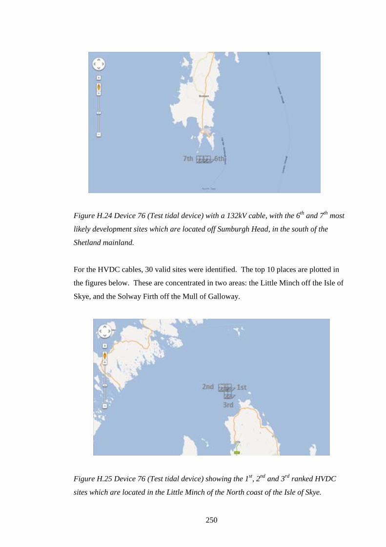
250

Figure H.24 Device 76 (Test tidal device) with a 132kV cable, with the 6th

and 7th

most

likely development sites which are located off Sumburgh Head, in the south of the

Shetland mainland.

For the HVDC cables, 30 valid sites were identified. The top 10 places are plotted in

the figures below. These are concentrated in two areas: the Little Minch off the Isle of

Skye, and the Solway Firth off the Mull of Galloway.

Figure H.25 Device 76 (Test tidal device) showing the 1st, 2

nd and 3

rd ranked HVDC

sites which are located in the Little Minch of the North coast of the Isle of Skye.

251

Figure H.26 Device 76 (Test tidal device), showing the 4th

to 10th

ranked HVDC sites

which are located off the Mull of Galloway.

Figure H.27 showing a GIS (MapInfo) plot for all sites found for Device 76 Test tidal

device.

H.2 Batch results, second run

For a summary of the second run methodology and results please refer to: 5.3 Batch

results after change to resource test logic (second run).

252


The results show for Device 5 (Pelamis) the top 4 sites are the same for a 33kV cable,

with the remaining 2 sites from the original 6 (North of Westray see Figure H.1, and

the northern most in the passage of Tiree, see Figure H.2) now not passing to the final

results. For a 132kV cable, only the site east of Shetland (see Figure H.3) and the site

west of Lewis (see Figure H.7) survived, these sites are now ranked1st and 2

nd (all) as

opposed to being 2nd

and 5th

originally. For a HVDC cable no valid sites were returned

in the second run.


For Device 75 (Test wave device) the top five, along with the 7th

9th

, 10th

33kV

positions have all now fallen, of which, the top four and the 7th

, 9th

, 10th

were all in the

highly tidal Falls of Warness in Orkney (see Figure H.10), with the last remaining being

in the Passage of Tiree (see Figure H.9). The new top 10 are displayed in Figures H.28

and H.29 below.


nd, 3

rd, 5

th, 6

th, and 9

th

ranked 33kV sites in the Passage of Tiree, and 8th

off Barra.

253


, 7th

and 10th

ranked 33kV

sites in the Orkney Isles.

For the 132 kV results the 2nd

4th

and 7th

sites (see Figure H.13) around North

Ronaldsay in Orkney have been lost, as have the 3rd

and 9th

sites (see Figure H.12) off

the south west Shetland mainland, along with the 1st site at the Out Skerries in Shetland.

The new top 4 is made up of sites that were already in the top 10 with the remaining

sites all new to the top 10, see Figures H.30 and H.31.


rd, 4

th, 6

th,7

th and 9

th ranked

132 kV sites off the west coast of the Isle of Lewis.

254


, 5th

and 10th

ranked 132kV

sites around the Shetland Isles.

For the HVDC cable, the previous rankings from 1st to 5

th remain. Positions 6

th, 7

th, 9

th

and 10th

have gone due to them being in the tidal areas (see Figures H.15 and H.16).

The original position 8th

is now 6th

in the latest run, with new 7th

to 10th

positions.

Figure H.32 Device 75 (Test wave device) showing the 1st to 10

th ranked HVDC sites off

the west coast of Harris and Lewis.

255


For device 76 (test tidal device) the alteration to the logic has marked effect with only 1

out of the previous 649 sites now passing the various tests to make it to the final

profit/loss result. This is mainly due to the model not finding favourable sheltered sites

as the resolution of the DTI data are not high enough within inland areas. The model is

now ruling out exposed tidal sites where there is a high wave regime, however, with the

resolution of the DTI data the model cannot find sheltered sites, which is a weakness of

the present model. The only site to pass to the final profit/loss result is high in the

Solway Firth off Annan. This site ranked 54th

out of the 444 33kV sites found in the

first run.

Figure H.33 Device 76 (Test tidal device) showing the only site to have passed to the

final profit/loss results, which is off Annan in the upper reaches of the Solway Firth.

As expected, no new sites were found, as no actual data have been changed to allow

this. The result were only ever going to be the sites found in the first run, minus the

sites identified with conflicting tidal or wave resource.

H.3 Batch results, third run

For a summary of the third run methodology and results please refer to: 5.4 Batch

results after changes, and additions to various database parameters (third run).

256


From the third run, with various changes made, there were no changes to the overall

results for Device 5. Again only 6 sites (4 for 33kV and 2 for 132kV) were found and

their rankings did not change.

H.3.2 Device 7 (OSPREY)

The additional data entered for this device has allowed for it to pass to the final

profit/loss indication results. The device has returned 6 sites: four 33kV and two

132kV.

Figure H.34 Device 7 (OSPREY) showing the 1st to 4

th (all) ranked 33kV sites in the

Orkney and Shetland Isles.

257

Figure H.35 Device 7 (OSPREY) showing the 1st and 2

nd (all) ranked 132kV sites off the

Isle of Skye and Mull respectively.

H 3.3 Device 13 (Wave Star)

The additional data entered for this device has allowed for it to pass to the final

profit/loss indication results. Device 13 (Wave Star) has come out very favourably,

with 253 sites identified.


th ranked 33kV sites off the east

coast off the Isle of Lewis, Dounreay, and around the Orkney Isles.

258

Figure H.37 Device 13 (Wave Star) showing the 1st, 2

nd, 3

rd and 6th ranked 132kV sites

off the island of Yell, Unst and Fetlar in the Shetland Isles.


and 7th

ranked 132kV sites off the

Buchan coast in the north east of Scotland.

259


, 8th

, 9th

, and 10th

ranked 132kV sites

off the west coast off the Isle of Lewis.


th ranked HVDC sites in

various locations around the western coast and isles.

260

Figure H.41 Device 13 (Wave Star) showing the entire 253 results plotted with the GIS

package MapInfo.

H.3.4 Device 45 (Marine Current Turbines)

The addition of additional device data and extra connection points has not allowed

Device 45 to produced any final profit/loss results. While there were positive

developments for all three physical attributes of : physical resource, distance from land,

depth, there did not all coincide at the same site, and hence no valid union file was

produced. A key reason for this was the device record stipulating 30 m of water (with

no lower or upper range), a relatively high resource required (2.83 ms-1), and some

issues with the data resolution as discussed earlier. This is made more difficult

considering the alteration to the code to overlook tidal sites with a conflicting wave

resource, which discounts many large areas with a high tidal resource.

H.3.5 Device 47 (TidE1)

The additional data entered for this device have allowed it to pass to the final profit/loss

indication results, returning a single 132kV result.

261

Figure H.42 Device 47 (TidE1) showing the 1st (only) ranked 132kV site off the

Northern Irish coast.

H.3.6 Device 56 (Hammerfest Strøm)

The additional data entered for this device have allowed for it to pass to the final

profit/loss indication results with 7 sites with a 132kV cable providing final results.

Figure H.43 Device 56 (Hammerfest Strøm) showing the 4th

to 7th

ranked 132kV sites

off the north coast of the Isle of Man.

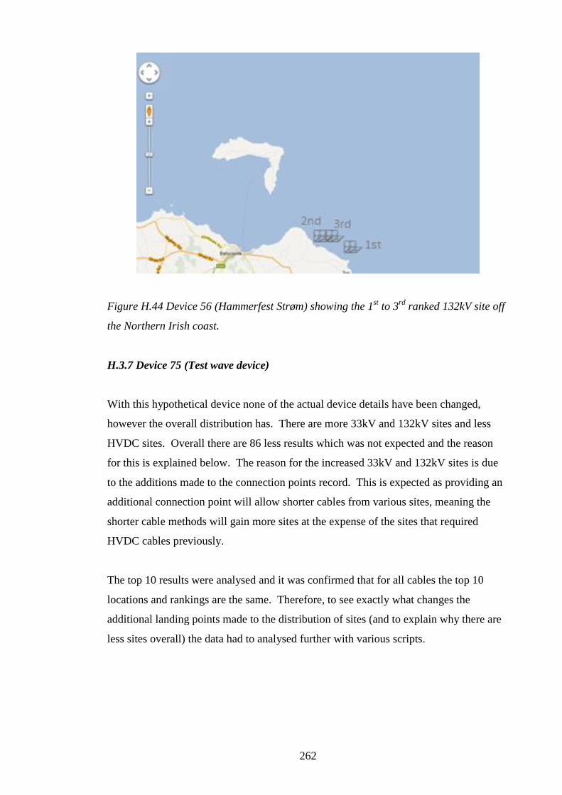
262

Figure H.44 Device 56 (Hammerfest Strøm) showing the 1st to 3

rd ranked 132kV site off

the Northern Irish coast.


With this hypothetical device none of the actual device details have been changed,

however the overall distribution has. There are more 33kV and 132kV sites and less

HVDC sites. Overall there are 86 less results which was not expected and the reason

for this is explained below. The reason for the increased 33kV and 132kV sites is due

to the additions made to the connection points record. This is expected as providing an

additional connection point will allow shorter cables from various sites, meaning the

shorter cable methods will gain more sites at the expense of the sites that required

HVDC cables previously.

The top 10 results were analysed and it was confirmed that for all cables the top 10

locations and rankings are the same. Therefore, to see exactly what changes the

additional landing points made to the distribution of sites (and to explain why there are

less sites overall) the data had to analysed further with various scripts.

263

Figure H.45 showing an overall distribution of device 75 for the second (left) and third

runs. At this resolution it is very difficult to spot the difference in device numbers,

however the distribution change of the sites per cost can be identified with careful

inspection which is the result of the newly added connection points (shown in blue) on

the east coast.

As Device 75 returned the most valid sites in the second and third runs, a supplementary

script was written to examine in more detail valid Device 75 sites with a 10 km2 area

around the two new landing points. In the case of the newly added Pentland Firth

landing point no new sites were identified in this area for any cable type. The reason for

this is that the area is a high tidal energy site, and the constraint of excluding wave

devices in such locations incorporated in the second batch run excluded any such

devices. At the second new landing point in the North Sea, the same 35 sites were found

for Device 75 in both second and third runs. The important difference however was the

change in the profit/loss indication results which show a reduction in cost (on average

17%) and a consequential increased profit/loss value for sites adjacent to the new

landing points.

264

Figure H.46 showing the new landing points at the centre of defined study areas in the

Pentland Firth (left yellow) and North Sea (right blue).

There is little difference in the actual profit/loss (cost) indication results for all sites in

this area, less than 1% in both runs between the top site and the 35th

site. However,

within this new connection point area for the third run, there is a lower cost distribution

between the top (1st) to bottom (35

th) sites compared to the second run, i.e. the site

profit/loss results return closer values in relation to each other than before. This change

in distribution can be explained by the fact all the sites can now be linked to a close

connection point via a 33kV cable, as opposed to a mainland point by a HVDC cable.

Another script was used to take a closer look at all the devices within the new North Sea

10 km test zone. From this the maximum and minimum cable values were stored to

enable further analysis of the same 35 Device 75 sites. It was established that the

maximum development scenario for the site and cable, showed a significantly lower

cost indication in the third run (with the insertion of the new connection point) than

previously. However, some of the values for the minimum development scenario were

actually lower for the HVDC cable (second run) as the cable attributes within the

database allows for a minimum of 200 MW to be installed for a HVDC cable rather

than 400 MW for a 33kV. The cost of the devices, equalling 200 (1 MW each) for the

minimum HVDC solution in the second run, was actually less than for the minimum

265

33kV solution using 400 (1 MW devices) in the third. It can also be established that the

device cost is also a factor when considering the maximum HVDC output which is 600

MW, compared to the 33kV 500 MW within the database. The device cost has been

shown to be significant in this exercise, as has the use of a particular cable with the

associated maximum and minimum devices (in which these are the two values used by

the model), as did the shorter allowed cable made available by the new connection

point.

A further script was then used to extract the “difference” result from the both datasets,

i.e. data that exists in one dataset but not the other, in order to explain why there are less

sites overall. The results show data entries that exist for Device 75 (all cable types) in

the second run that did not exist in the third run. This totalled 95, with a corresponding

9 entries in the third run set that does not exist in the second. This means 95 sites were

found in second run were not available in the third run, and 9 new sites found in run

three were not available in run two.

Figure H.47 showing the data difference between the second and third runs (left), and

third and second runs (right). Each point indicates an individual site. 95 sites were

identified in the second run which were not found in the third run, and 9 sites were

identified in the third run which were not in the second run. These results point to a

potential error in the coding/data used.

The circular array of points in the MapInfo display in Figure H.47 represents the

difference between the two batch runs which demonstrates the importance of using

differential data to check the validity of results. The feature in the display was not

expected and indicated an issue with the data entries within the database. Inspection of

the cable dataset, indicated that the defined distances for the 33kv cables were: 0-29 km,

266

30-49 km for 132 kV, and above 50 km for HVDC cables. This meant that there were

void areas between 29-30 km and 49-50 km. For example, one of the newly identified

sites in the third run is 28.8 km east of the Pentland Firth test landing point to the east of

Orkney. This site in the second run would have been out with the bounds of a 33kv

cable to Kirkwall power station as at 29.67 km distance, it was greater than the upper

threshold for the 33 kV cable, and too short for the 132kV cable. 6 more of the sites

further to the east of the new Pentland Firth connection point were in the previous

distance region between the 132kV and HVDC void for Kirkwall Power Station and

Flotta landing points.

The two remaining new sites within the third run were 35.8 km from the newly added

North Sea test landing point. Before the North Sea landing point was added, the closest

landing point was St Fergus on the Buchan coast which was 49.55 km away, again in

between the distance of a 132kV cable and a HVDC cable. The logic is working

correctly in the model, however this is not an ideal situation as valid sites are being

missed. Therefore, the data for the cables has been changed so there is no gap between

the cable types and to ensure sites are not missed.


With this hypothetical device none of the actual device details have been changed, and

this has not changed the overall result pattern in this run. There was only one result

from the second batch run, which was found to be the unchanged in the third run.

267

APPENDIX I, LIST OF DEVICES MODEL USES

Devices processed by model, in form: Device ID number, name of device

(company/developer)

I.1 Wave Devices

1 WaveDragon (Nissum Bredning), Wave Dragon ApS

2 WaveDragon (North Sea Design), Wave Dragon ApS

3 WaveDragon (36 kW/m Design), Wave Dragon ApS

4 Wave Dragon (Full Scale), Wave Dragon ApS

5 Pelamis, Ocean Power Delivery Limited (OPD)

6 EB Frond 0.5 MW, The Engineering Business Limited (EB)

7 OSPREY, Wavegen

8 OSPREY2, Wavegen

9 Mighty Whale, Japan Marine Science and Technology Centre (JAMSTEC)

10 Archimedes WaveSwing (AWS) Demonstration(2 MW), Archimedes

WaveSwing (AWS) II BV

11 Archimedes WaveSwing (AWS) (6 MW) Archimedes WaveSwing (AWS) II BV

12 Floating Wave Power Vessel (FWPV), Sea Power International AB

13 Wave Star (North Sea Design)

14 Green Cat Turbine (GCT), Green Cat Renewables Ltd

15 Wave Rotor, Evelop BV

16 WaveRoller, Advanced Wave Energy (AW-Energy) Oy

17 Offshore Wave Energy Device (OWEL), Offshore Wave Energy Limited

18 SEAREV 0.5, Lecole Centrale de Nantes (Central School of Nantes)

19 WECA PDP500 (Wave Energy Conversion Activator-Pressure Dynamics

Processor), DAEDALUS Informatics Ltd

20 Salter/Edinburgh Duck, Edinburgh University (The Wave Power Group)

21 PS Frog, Lancaster University Renewable Energy Group

22 Sea Clam, Coventry University

23 Cockerell Raft, Wavepower Limited (Sir Christopher Cockerell)

24 IPS Buoy, Interproject Service (IPS) AB

25 Sloped IPS Buoy, Edinburgh University (The Wave Power Group)

268

26 PowerBuoy, Ocean Power Technologies, Inc. (OPT)

27 Spurboy, Embley Energy Ltd

28 Wavebob, Clearpower Technology Limited

29 Swedish Hosepump, Technocean (Sweden)

30 McCabe Wave Pump, Hydam Technologies Ltd (Peter McCabe)

31 CETO Wave Energy Converter, Seapower Pacific PTY LTD

32 CETO Wave Energy Converter Full Scale, Seapower Pacific PTY LTD

33 Combined Energy System (CES), Ocean Motion International (OMI)

34 Slot-Cone Generator (SSG) Breakwater, WAVEenergyAS

35 Manchester Bobber, The University of Manchester Intellectual Property

36 C-Wave 1 MW, C-Wave Limited

37 AquaBuOY, AquaEnergy Group Limited

38 Float Pump, Danish Wave Power (DWP)

39 Bolgepumpen, Danish Maritime Institute

40 Hanstholm Buoy, Not Known

41 Oyster, AQUAMARINE POWER

42 Neptune Triton, Neptune Renewable Energy Ltd

43 bioWave, BioPower Systems Pty Ltd

44 Waveberg, Waveberg Development Limited

75 Test Wave Device, Hypothetical Test Company

I.2 Tidal Devices

45 Marine Current Turbines, Marine Current Turbines Limited (MCT)

46 Marine Current Turbines, Marine Current Turbines Limited (MCT)

47 TidE1, SMD Hydrovison

48 Stingray, The Engineering Business Limited (EB)

49 Stingray 2nd Generation, The Engineering Business Limited (EB)

50 Brian the Snail, Robert Gordon University (RGU)

51 Exim Stromturbiner, Sea Power International AB

52 Tidal Fence (Micro), Blue Energy Canada Inc

53 Venturi Energy Generating Apparatus (VEGA), Nova Energy Limited

54 Underwater Kite, Underwater Electric Kite (UEK)

55 Gorlov Helical Turbine, GCK Technology Inc

269

56 Hammerfest Strøm, Hammerfest Strøm

57 Ramsey sound Turbine, Tidal Hydraulic Generators Ltd

58 OpenCenter Submerged Composite Turbine, OpenHydro

59 TidalStream Semi-Submersible Turbine 2x1 MW Rotor, TidalStream

60 TidalStream Semi-Submersible Turbine 2x2 MW Rotor, TidalStream

61 SwanTurbine, SwanTurbines Limited

62 Offshore Energy Platform (KESC Bowsprit Tidal Generator), Kinetic Energy

Systems, Inc.

63 KESC Bowsprit Tidal Generator, Kinetic Energy Systems Inc.

64 Tidal Generation Turbine, Tidal Generation Limited

65 Verdant Power Turbine, Verdant Power, LLC

66 Neptune Proteus Tidal Power Pontoon, Scottish and Southern Electric

67 Rotech (Lunar) Tidal Turbine (RTT) (1 MW), Lunar Energy Limited

68 Rotech (Lunar) Tidal Turbine (RTT) (2 MW), Lunar Energy Limited

69 Race Rocks, Pearson Collage Race Rocks Project

70 ENERMAR, Ponte di Archimede S.p.A. & Dpt of Aeronautical Eng, University

of Naples

71 MYTHOS, Ponte di Archimede S.p.A. & Dpt of Aeronautical Eng, University of

Naples

72 Loch Linnie Device, Scottish Nuclear, IT Power, and NEL

73 bioStream, BioPower Systems Pty Ltd

74 Leslie Pump, George Leslie, The Leslie Pump

76 Test Tidal Device, Hypothetical Test Company

I.3 Devices identified, but not processed by model due to insufficient data, in form:

name of device, company/developer.

Wave Devices

WavePlane, WavePlane Production A/S

Oscillating Device, Arvid Nesheim

Waterturbine, Arvid Nesheim

Wave Plunger, Danish Maritime Institute

WaveMill (Self Contained), Wavemill Energy Corp (WEC)

270

Seawave Slot-Cone (SSG) Offshore Fixed Device, WAVEenergyAS

Ocean Wave Energy Converter (OWEC), Ocean Wave Energy Company (OWECo)

Oscillating Wave Surge Converter (OWSC), Queen's University Belfast and

Manchester Metropolitian University

WaveMaster, Ocean WaveMaster Limited

DAM-ATOLL, Lockheed Missiles and Space Company

Pneumatically Stabilized Platform (PSP), Float Incorporated

Bristol Cylinder, Bristol University& Sir Robert McAlpine

HRS Rectifier/Russell Lock, Hydraulics Research Station and Robert Russell

Kaimei, Japan Marine Science and Technology Centre (JAMSTEC)

Backward Bent Duct Buoy, Ryokuseisha Corporation

Wave Rider, SeaVolt Technologies

Wavemill Open Buoy Design, Wavemill Energy Corp (WEC)

Directly Driven Linear Generators (DDLG), Seabased Energy AB

Snapper, Ed Spooner & New and Renewable Energy Centre (NaREC)

SEADOG Pump, Independent Natural Resources, Inc.(INRI)

WaveBlanket, WindWavesAndSun.com

SyncWave Power Resonator, SyncWave Energy Inc

Polo, Edinburgh University (The Wave Power Group)

FO³ SEEWEC, SEEWEC

Tidal Devices

Rochester Venturi, HydroVenturi Ltd

Scotrenewables Turbine, ScotRenewables

GENTEC Venturi, Greenheat Systems

Water Wall Turbine (Tidal), Water Wall Turbine Inc.

Tidal Fence (Blue Energy Power System) 500 MW, Blue Energy Canada Inc.

Tidal Fence (Mega Power System) 10 MW, Blue Energy Canada Inc.

271

APPENDIX J, PSEUDO CODE OF MODEL (AS BUILT)

FUNCTIONS, BATCH OPERATION

J.1 Determining a spatial distribution for each device determined by water depth

Declare dataStructure as column (520) with 4 digits per field

Declare outputStructure as column (520) with 2 digits per field

Open DTI Water Depth file

While Device.Name in Database Device Table <>End of File

If (Device.Minimum Depth and Maximum Depth <>“”) Then

Open Device by Depth file for Random Access

For each record row (j) (j = 1 to 450)

Read into dataStructure the (j) record of the DTI Water Depth file

For each column (i) (i = 0 to 519)

If (dataStructure.column(i) <> “NA”) Then

If (dataStructure.column(i) >= Device.Max Depth &<= Device.Min

Depth) then

outputStructure.column(i) = “1”

Else


End if

Else

outputStructure(j).column(i) = “NA”

End if

Increment i

Write outputStructure to (j) record of the Device by Depth file

Increment j

ElseIF (Device.Ideal Depth <> “”) Then


Read into dataStructure the (j) record of the DTI Water Depth file



If (dataStructure.column(i) = Device.IdealDepth) Then


Else


End if

Else

outputStructure(j).column(i) = “NA”

End if

Increment i

Write outputStructure to (j) record of theDevice by Depth file

Increment j

End if

Close Device by Depth file

Move to Next Device

Close DTI Water Depth file

272

J.2 Determining a spatial distribution for each device determined by resource

Declare dataStructure1 as column (520) with 5 digits per field





Open DTI:Winter Mean Wave Power, Summer Mean Wave Power, Mean Spring Peak

Flow, Mean Neap Peak Flow files

While Device.Name in Database Device Table <> End of File

If (Device.Wave Climate <> “”& Device.Type = “WAVE”) Then

Open Device by Resource file for Random Access


Read into dataStructure1 the (j) record of the DTI Winter Mean Wave Power (j)

Read into dataStructure2 the(j) record of the DTI Summer Mean Wave Power (j)


If (dataStructure1.column(i)<> “NA”) Then

If (devices.Wave Climate <= dataStructure1.column(i) and >=

dataStructure2.column(i) ) then


Else


End if

Else

outpurtStructure.column(i) = “NA”

End if

Increment i

Write outputStructure to (j) record of the Device by Resource file

Increment j

ElseIF (Device.Tidal Climate<> “”& Device.Type = “TIDAL”) Then


Read into dataStructure3 the (j) record of the DTI Mean Spring Peak Flow file

Read into dataStructure4 (j) record of the DTI Mean Neap Peak Flow file

For each column (j) (i = 0 to 519)

If (dataStructure3.column(i) <> “NA”) Then

If (Device.Tidal Climate <= dataStructure3.column(i) &>=

dataStructure4.column(i)) Then


Else


End if

Else

outputStructure.column(i) = “NA”

End if

Increment i

Write outputStructure to (j) record of the Device by Resource file

Increment j

End if

Close Device by Resource file

Move to Next Device

273

Close DTI: Winter Mean Wave Power, Summer Mean Wave Power, Mean Spring

Peak Flow, Mean Neap Peak Flow files

J.3 Determining a spatial distribution for each device determined by distance to

land



Open DTI Distance to Land file


If (Device.Distance to Land<> “”) Then

Open Device by Distance file for Random Access


Read into dataStructure the (j) record of the DTI Distance to Land file



If (dataStructure.column(i) to km <= Device.Distance to land) then


Else


End if

Else

outpurStructure(j).column(i) = “NA”

End if

Increment i

Write outputStructure to (j) record of the Device by Distance file

Increment j

End if

Close Device by Distance file

Move to Next Device

Close DTI Distance to Land file

J.4 Determining an overall spatial distribution for each device determined by

water depth, resource, and distance to land






If (Device by Depth, Resource and Distance files<> “”) then

Open Device by: Depth, Resource, Distance files

Open Device by Distance file for Random Access


Read into dataStructure the (j) record of the DTI Distance to Land file

274



If (dataStructure1.column(i) = “1” & dataStructure2.column(i) = “1” &

dataStructure3.column(i) = “1”) then


Else


End if

Else

outpurStructure(j).column(i) = “NA”

End if

Increment i

Write outputStructure to (j) record of the Device by Union file

Increment j

End if

Close Device by Union file

Close DTI Distance to Land file

Move to Next Device

J.5 Constructing a distance matrix from each site to closest power station


Declare outputStructure1 as column (520) with 5 digits per field


Open DTI Annual Mean Wave Height file

Open Power Distance file for Random Access

Open Power ID file for Random Access

Set Latitude Seconds to 221370, location of 61° 29.5’ North


Set Longitude Seconds to -34515, location of 9° 35’ 25’’ West

Read into dataStructure the (j) record of the DTI Annual Mean Wave Height


Set shortestDistance to10000

Set boolean marker to false


outputStructure1.column(i) = “NA”


Else

While Power Station.Name in Database Device Table <> End of File

Calculate Latitude Difference from Latitude Seconds – Power

Stations.LatitudeSeconds

Calculate Longitude Difference from Longitude Seconds – Power

Stations.Longitude Seconds

Save Power Stations.Latitude Seconds as Holding Degree Value

Call Calculate Distance Method (passing: Latitude Difference, Longitude

Difference, Holding Degree Value, Latitude Seconds) Returning Overall

Distance

275

If (Overall Distance < Shortest Distance) Then

While Cables in Database <> End of File

If (Overall Distance > Cables.Min Length and < Cables.Shortest Length)

Then

If (Cables.Max Output < Power Station.Capacity) then

Shortest Distance = Overall Distance

Shortest Location = Power Stations.ID

Set boolean marker to true

End if

End if

Move to next Cable

End if

Move to next Power Station

If (marker =true) then

outputStructure1.column(i) = Shortest Distance

outputStructure2.column(i) = Shortest Location

End if

outputStructure1.column(i) = na

outputStructure2.column(i) = na

End if

Increment Longitude Seconds by 90

Increment i

Write outputStructure1 to (j) record of Power Distance file

Write outputStructure2 to (j) record of Power ID file

Decrement Latitude Seconds by 60

Increment j

Close DTI Annual Mean Wave Height file

Close Power Distance file

Close Power ID file

J.6 Construct a distance matrix from each site to closest port

This method is very similar to that of J.5 Constructing a distance matrix from each site

to closest power station. The main difference is this method is calculating the port

datasets. There is also a slight difference in logic as this method does not look at a

spare capacity figure as with the power stations, and that the method saves the first port

as a distance benchmark which is not undertaken for power stations.




Open DTI Annual Mean Wave Height file

Open Port Distance file for Random Access

Open Port ID file for Random Access

Set Latitude Seconds to 221370, location of 61° 29.5’ North


276

Set Longitude Seconds to -34515, Location of 9° 35’ 25’’ West

Read into dataStructure the (j) record of the DTI Annual Mean Wave Height


Set boolean marker to false




Else

While Port.Name in Database Device Table <> End of File

Calculate Latitude Difference from Latitude Seconds – Port.LatitudeSeconds

Calculate Longitude Difference from Longitude Seconds – Port.Longitude

Seconds

Save Port.Latitude Seconds as Holding Degree Value

Call Calculate Distance Method (passing: Latitude Difference, Longitude

Difference, Holding Degree Value, Latitude Seconds) Returning Overall

Distance

If (marker = True) Then

If (Overall Distance < Shortest Distance) Then


Shortest Location = Port.ID

End if

Else


Shortest Location = Port.ID

End if

Set boolean marker to true

Move to next Port Station

outputStructure1.column(i) = Shortest Distance

outputStructure2.column(i) = Shortest Location

End if

Increment Longitude Seconds by 90

Increment i

Write outputStructure1 to (j) record of Port Distance file

Write outputStructure2 to (j) record of Port ID file

Decrement Latitude Seconds by 60

Increment j

Close DTI Annual Mean Wave Height file

Close Port Distance file

Close Port ID file

J.7 Calculate cable costs for each site against valid location for each device



Declare CableCostArray array (0 to 2) as column (520) with 9 digits per field

Declare CurrentFileName array (0 to 2) as String


Open Device by Union file

If (Device by Union file <> “”) Then

277

Open Power Distance file

Open Cable Costs 33kV file for Random Access as CurrentFileName(0)

Open Cable Costs 132kV file for Random Access as CurrentFileName(1)

Open Cable Costs HVDC file for Random Access as CurrentFileName(2)


Read into dataStructure1 the (j) record of the Device by Union file

Read into dataStructure1 the (j) record of thePower Distance file


If (dataStructure1.column(i) = “NA”) Then

For each x (x = 0 to 2)

cableCostArray(x).column(i) = “NA”

Next x

If (dataStructure1.column(i) = “na”) Then


cableCostArray(x).column(i) = “na”

Next x

Elseif (dataStructure1.column(i) = “0”) Then


cableCostArray(x).column(i) = “0”

Next x

Else

Set count to 0

While Cables.Name in Database Device Table <> End of File

If (theStructure2.column(i) to km >= Cables.Min Length km) &

theStructure2.column(i) to kilometers<= Cables.Max Length km) Then

cableCostArray(count).column(i) = theStructure2.column(i) to

km * Cables.Overall Cost

Else

cableCostArray(count).column(i) = “na”

End if

increment count

Move to next Cable

End if

Increment i


Write cableCostArray(x) to (j) record of CurrentFileName(x)

Increment x

Increment j


Close Cable Costs 33kV file for Random Access

Close Cable Costs 132kV file for Random Access

Close Cable Costs HVDC file for Random Access

Move to next Device

278

J.8 Calculate the number of devices required and device output at a given site



Declare CableInputsArrayarray (0 to 5) as column (520) with 5 digits per field

Declare OutputValueArray array (0 to 5) as column (520) with 3 digits per field

DecareouputFile array (0 to 5) as String



If (Device by Union file<> “”) Then

Open Device by Union file as CurrentFileName(0)

Open Power Distance file as CurrentFileName(1)

Open Device 33kV Min Number file for Random Access as CurrentFileName(2)

Open Device 33kV Max Number file for Random Access as CurrentFileName(3)

Open Device 132kV Min Number file for Random Access as CurrentFileName(4)

Open Device 132kV Max Number file for Random Access as CurrentFileName(5)

Open Device HVDC Min Number file for Random Access as CurrentFileName(6)

Open Device HVDC Max Number file for Random Access as CurrentFileName(7)

Open Device 33kV Min Output Number file for Random Access as outputFile(0)

Open Device 33kV Max Output Number file for Random Access as outputFile(1)

Open Device 132kV Min Output Number file for Random Access as outputFile(2)

Open Device 132kV Max Output Number file for Random Access as outputFile(3)

Open Device HVDC Min Output Number file for Random Access as outputFile(4)

Open Device HVDC Max Output Number file for Random Access as outputFile(5)



Read into dataStructure2 the (j) record of the Power Distance file



cableInputsArray(x).column(i) =””

outputValueArray(x).column(i) =””

Next x



cableInputsArray(x).column(i) = “NA”

outputValueArray(x).column(i) = “NA”

Next x

Elseif (dataStructure1.column(i) <> “0” or dataStructure2.colum(i) = “na”) Then


cableInputsArray(x).column(i) = “na”

outputValueArray(x).column(i) = “na”

Next x

Else

Set count to 0

While Power Cables in Database Device Table <> End of File

If (Cables.Min Length <theStructure2.column(i) to km &

Cables.Max Length km > theStructure2.column(i) to kilometers Then

cableInputsArray(count).column(i) = Cables.Min Output /

Devices.output

279

cableInputsArray(count +1).column(i) = Cables.Max Output /

Devices.output

outputValueArray (count).column(i) =

cableInputsArray(count).column(i) * Devices.output

outputValueArray (count +1).column(i) =

cableInputsArray(count +1).column(i) * Devices.output

Else

cableInputsArray(count).column(i) = “na”

cableInputsArray(count +1).column(i) = “na”

outputValueArray(count).column(i) = “na”

outputValueArray(count +1).column(i) = “na”

End if

increment count by 2

Move to next Cable

End if

Increment i


Write cableInputsArray(x) to (j) record of CurrentFileName(x +2)

Write outputValueArray(x) to (j) record of outputFile(x)

Increment x

Increment j



Close Device 33kV Min Number file

Close Device 33kV Max Number file



Close Device HVDC Min Number file

Close Device HVDC Max Number file

Close Device 33kV Min Output Number file

Close Device 33kV Max Output Number file

Close Device 132kV Min Output Number file

Close Device 132kV Max Output Number file

Close Device HVDC Min Output Number file

Close Device HVDC Max Output Number file

Move to next Device

J.9 Calculate the device cost for a given valid site

Declare dataStructure array (0 to 5) as column (520) with 5 digits per field

Declare deviceCostArray array (0 to 5) as column (520) with 9 digits per field

DecareoutputFile array (0 to 5) as String



If (Device 33kV Min Number file <> “”) Then

Set Device 33kV Min Number file as CurrentFileName(0)

Set Device 33kV Max Number file as CurrentFileName(1)

Set Device 132kV Min Number file as CurrentFileName(2)

280

Set Device 132kV Max Number file as CurrentFileName(3)

Set Device HVDC Min Number file as CurrentFileName(4)

Set Device HVDC Max Number file as CurrentFileName(5)

Set Device 33kV Min Cost file for Random Access as outputFile(0)

Set Device 33kV Max Cost file for Random Access as outputFile(1)

Set Device 132kV Min Cost file for Random Access as outputFile(2)

Set Device 132kV Max Cost file for Random Access as outputFile(3)

Set Device HVDC Min Cost file for Random Access as outputFile(4)

Set Device HVDC Max Cost file for Random Access as outputFile(5)


Open CurrentFileName(x)

Open outputFile(x)


Read into dataStructure(x) the (j) record of the file set at CurrentFileName(x)


deviceCostArray(x).column(i) =””

If (Devices.device cost > 0) Then

If (dataStructure(x).column(i) = “NA”) Then

deviceCostArray(x).column(i) = “NA”

Elseif (dataStructure(x).column(i) = “na”) Then

deviceCostArray(x).column(i) = “na”

Else

deviceCostArray(x).column(i) = Devices.device cost *

dataStructure(x).column(i)

End if

Else

deviceCostArray(x).column(i) = “na”

End if

Increment i

Write deviceCostArray(x) to (j) record of outputFile(x)

Increment j

Close outputFile(x)

Close CurrentFileName(x)

Increment x

End if

Move to next Device

J.10 Add device costs to cable costs

Declare dataStructure1 array (0 to 2) as column (520) with 9 digits per field


Declare costArray array (0 to 8) as column (520) with 9 digits per field

Declare CurrentFileName1 array (0 to 2) as String


Declare outputFile array (8) as String


If (Device 33kV Min Cost file <> “”) Then

Open Device 33kV Cable Cost as CurrentFileName1(0)

281

Open Device 132kV Cable Cost as CurrentFileName1(1)

Open Device HVDC Cable Cost file as CurrentFileName1(2)

Open Device 33kV Min Cost file as CurrentFileName2(0)

Open Device 33kV Max Cost file as CurrentFileName2(1)

Open Device 132kV Min Cost file as CurrentFileName2(2)

Open Device 132kV Max Cost file as CurrentFileName2(3)

Open Device HVDC Min Cost file as CurrentFileName2(4)

Open Device HVDC Max Cost file as CurrentFileName2(5)

Open Device/Cable 33kV Min Cost file for Random Access as outputFile(0)

Open Device/Cable 33kV Max Cost file for Random Access as outputFile(1)

Open Device/Cable 132kV Min Cost file for Random Access as outputFile(2)

Open Device/Cable 132kV Max Cost file for Random Access as outputFile(3)

Open Device/Cable HVDC Min Cost file for Random Access as outputFile(4)

Open Device/Cable HVDC Max Cost file for Random Access as outputFile(5)

Set Count to 0



Read into dataStructure1(x) the (j) record of the file set at

CurrentFileName(x)

Read into dataStructure2 (count) the (j) record of the file set at

CurrentFileName2(count)

Read into dataStructure2 (count +1) the (j) record of the file set at

CurrentFileName2(count +1)


costArray(count).column(i) = “”

costArray(count +1).column(i) = “”

If (dataStructure2(count).column(i) = “NA”) Then

costArray(count).column(i) = “NA”

costArray(count +1).column(i) = “NA”

Else if (dataStructure2(count).column(i) = “na”) Then

costArray(count).column(i) = “na”

costArray(count +1).column(i) = “na”

Else

costArray(count).column(i) = dataStructure1(x).column(i) +

dataStructure2(count).column(i)

costArray(count +1).column(i) = dataStructure1(x).column(i) +

dataStructure2(count +1).column(i)

End if

Increment i

Write CostArray(count) to (j) record of outputFile (count)

Write CostArray(count +1) to (j) record of outputFile (count +1)

Increment j

Increment count by 2

Increment x

Close Device 33kV Cable Cost file

Close Device 132kV Cable Cost file

Close Device HVDC Cable Cost file

282

Close Device 33kV Min Cost file

Close Device 33kV Max Cost file

Close Device 132kV Min Cost file

Close Device 132kV Max Cost file

Close Device HVDC Min Cost file

Close Device HVDC Max Cost file

Close Device/Cable 33kV Min Cost file

Close Device/Cable 33kV Max Cost file

Close Device/Cable 132kV Min Cost file

Close Device/Cable 132kV Max Cost file

Close Device/Cable HVDC Min Cost file

Close Device/Cable HVDC Max Cost file

End if

Move to next Device

J.11 Calculate revenue at each site for each valid device


Declare valueArray array (0 to 5) as column (520) with 9 digits per field


Declare OutputFile array (0 to 5) as String

While ModelData <> End of File

If (ModelData.Name = “Unit price of electricity”) Then

UnitPriceOfElec = ModelData.value

End if

Move to next ModelData


If (Device 33kV Min Number file <> “”) Then

Open Device 33kV Min Number file as CurrentFileName(0)

Open Device 33kV Max Number file as CurrentFileName(1)



Open Device HVDC Min Number file as CurrentFileName(4)

Open Device HVDC Max Number file as CurrentFileName(5)

Open Device Revenue 33kV Min Income file for Random Access as outputFile(0)

Open Device Revenue 33kV Max Income file for Random Access as outputFile(1)

Open Device Revenue 132kV Min Income file for Random Access as outputFile(2)

Open Device Revenue 132kV Max Income file for Random Access as outputFile(3)

Open Device Revenue HVDC Min Income file for Random Access as outputFile(4)

Open Device Revenue HVDC Max Income file for Random Access as outputFile(5)



Read into dataStructure(x) the (j) record of the file set at CurrentFileName(x)


valueArray(count).column(i) = “”


283

valueArray(x).column(i) = “NA”

Else if (dataStructure(x).column(i) = “na”) Then

valueArray(x).column(i) = “na”

Else

valueArray(x).column(i) = dataStructure(x).column(i) *

UnitPriceOfElec

End if

Increment i

Write valueArray(x) to (j) record of outputFile (x)

Increment j

Increment x







Close Device Revenue 33kV Min Income file

Close Device Revenue 33kV Max Income file



Close Device Revenue HVDC Min Income file

Close Device Revenue HVDC Max Income file

End if

Move to next Device

J.12 Calculate installation depth factor for each site




Declare valueArray as column (520) with 3 digits per field


If (Device by Union file <> “”) Then

Open Device by Union file

Open DTI Water Depth file

Open Installation Depth Factor file for Random Access



Read into dataStructure2 the (j) record of the DTI Water Depth file


valueArray.column(i) = “”


valueArray.column(i) = “NA”

Else if (dataStructure1.column(i) = “na”) Then

valueArray.column(i) = “na”

Else

While DepthFactor table in Database <> End of File

If (dataStructure2.column(i) <= DepthFactor.Depth&

284

dataStructure2.column(i) >= DepthFactor.Depth2) Then

valueArray.column(i) = DepthFactor.Factor

End if

Move to next DepthFactor

End if

Increment i

Write valueArray to (j) record of Installation Depth Factor file

Increment j

End if


Close DTI Water Depth file

Close Installation Depth Factor file

Move to next Device

J.13 Calculate installation distance factor for each site

For the logic of this method please refer to: J.12 Calculate installation depth factor for

each site above. The only differences in the two methods is the output file name

(Installation Distance Factor file), the database table name which is DistanceFactor

rather than DepthFactor and the variable names that associated with the Database tables,

i.e. Depth Factor.Depth would read DistanceFactor.Distance. To calculate the factor the

Port Distance file is used rather than the DTI Water Depth file.

J.14 Calculate overall installation costs







If (Device Installation Depth Factor File <> “”) Then





Open Device HVDC Min Number file as CurrentFileName(4)

Open Device HVDC Max Number file as CurrentFileName(5)

Open Device Installation Depth Factor file as CurrentFileName(6)

Open Device Installation Distance Factor file as CurrentFileName(7)

Open Device 33kV Min Installation Cost file for Random Access as outputFile(0)

Open Device 33kV Max Installation Cost file for Random Access as outputFile(1)

285

Open Device 132kV Min Installation Cost file for Random Access as outputFile(2)

Open Device 132kV Max Installation Cost file for Random Access as outputFile(3)

Open Device HVDC Min Installation Cost file for Random Access as outputFile(4)

Open Device HVDC Max Installation Cost file for Random Access as outputFile(5)

While MooringFactor () End of File

If (MooringFactor.Method = Devices.Mooring Type Then

numberOfDays = MooringFactor.Factor

End if

Move to next ModelData



Read into dataStructure1(0) the (j) record of the file set at CurrentFileName(6)

Read into dataStructure1(1) the (j) record of the file set at CurrentFileName(7)

Read into dataStructure2 the (j) record of the file set at CurrentFileName(x)


valueArray(x).column(i) = “”

If (dataStructure2(x).column(i) = “NA”) Then


Else if (dataStructure2(x).column(i) = “na”) Then


Else

If (Devices.Daily Installation Cost <> “”) Then

valueArray(x).column(i) = dataStructure2(x).column(i) *

Devices.Daily Installation Cost * numberOfDays *

dataStructure1(0).column(i) * dataStructure1(1).column(i)

Else


End if

End if

Increment i


Increment j

Increment x







Close Device Installation Depth Factor file

Close Device Installation Distance Factor file

Close Device 33kV Min Installation Cost file

Close Device 33kV Max Installation Cost file



Close Device HVDC Min Installation Cost file

Close Device HVDC Max Installation Cost file

End if

Move to next Device

286

J.15 Add installation costs to device and cable costs








If (Device 33kV Min Installation Cost file <> “”) Then

Open Device 33kV Min Installation Cost file as CurrentFileName1(0)

Open Device 33kV Max Installation Cost file as CurrentFileName1(1)

Open Device 132kV Min Installation Cost file as CurrentFileName1(2)

Open Device 132kV Max Installation Cost file as CurrentFileName1(3)

Open Device HVDC Min Installation Cost file as CurrentFileName1(4)

Open Device HVDC Max Installation Cost file as CurrentFileName1(5)

Open Device 33kV Min Device\Cable Cost file as CurrentFileName2(0)

Open Device 33kV MaxDevice\Cable Cost file as CurrentFileName2(1)

Open Device 132kV Min Device\Cable Cost file as CurrentFileName2(2)

Open Device 132kV Max Device\Cable Cost file as CurrentFileName2(3)

Open Device HVDC Min Device\Cable Cost file as CurrentFileName2(4)

Open Device HVDC Max Device\Cable Cost file as CurrentFileName2(5)

Open Device 33kV Min Overall Costs file for Random Access as outputFile(0)

Open Device 33kV Max Overall Costs file for Random Access as outputFile(1)

Open Device 132kV Min Overall Costs file for Random Access as outputFile(2)

Open Device 132kV Max Overall Costs file for Random Access as outputFile(3)

Open Device HVDC Min Overall Costs file for Random Access as outputFile(4)

Open Device HVDC Max Overall Costs file for Random Access as outputFile(5)



Read into dataStructure1 the (j) record of the file set at CurrentFileName1(x)

Read into dataStructure2 the (j) record of the file set at CurrentFileName2(x)



If (dataStructure2(x).column(i) = “NA”) Then


Else if (dataStructure2(x).column(i) = “na”) Then


Else

valueArray(x).column(i) = dataStructure1(x).column(j) +

dataStructure2(x).column(j)

End if

Increment i


Increment j

Increment x

287





Close Device HVDC Min Installation Cost file

Close Device HVDC Max Installation Cost file

Close Device 33kV Min Device\Cable Cost file

Close Device 33kV MaxDevice\Cable Cost file

Close Device 132kV Min Device\Cable Cost file

Close Device 132kV Max Device\Cable Cost file

Close Device HVDC Min Device\Cable Cost file

Close Device HVDC Max Device\Cable Cost file

Close Device 33kV Min Overall Costs file

Close Device 33kV Max Overall Costs file



Close Device HVDC Min Overall Costs file

Close Device HVDC Max Overall Costs file

End if

Move to next Device

J.16 Determine profit/loss for each valid device at each valid site







If (Device 33kV Min Overall Costs file <> “”) Then

Open Device 33kV Min Overall Costs file as CurrentFileName1(0)

Open Device 33kV Max Overall Costs file as CurrentFileName1(1)

Open Device 132kV Min Overall Costs file as CurrentFileName1(2)

Open Device 132kV Max Overall Costs file as CurrentFileName1(3)

Open Device HVDC Min Overall Costs file as CurrentFileName1(4)

Open Device HVDC Max Overall Costs file as CurrentFileName1(5)

Open Device Revenue 33kV Min Income file as CurrentFileName2(0)

Open Device Revenue 33kV MaxIncome file as CurrentFileName2(1)

Open Device Revenue 132kV Min Income file as CurrentFileName2(2)

Open Device Revenue 132kV Max Income file as CurrentFileName2(3)

Open Device Revenue HVDC Min Income file as CurrentFileName2(4)

Open Device Revenue HVDC Max Income file as CurrentFileName2(5)

Open Device 33kV Min Profit Loss file for Random Access as outputFile(0)

Open Device 33kV Max Profit Loss file for Random Access as outputFile(1)

Open Device 132kV Min Profit Loss file for Random Access as outputFile(2)

Open Device 132kV Max Profit Loss file for Random Access as outputFile(3)

Open Device HVDC Min Profit Loss file for Random Access as outputFile(4)

Open Device HVDC Max Profit Loss file for Random Access as outputFile(5)

288



Read into dataStructure(x) the (j) record of the file set at CurrentFileName1(x)

Read into dataStructure (x +6) the (j) record of the file set at

CurrentFileName2(x +6)





Else if (dataStructure(x).column(i) = “na”) Then


Else

valueArray(x).column(i) = dataStructure(x +6).column(j) -

dataStructure(x).column(j)

End if

Increment i


Increment j

Increment x

Close Device 33kV Min Overall Costs file as CurrentFileName1(0)




Close Device HVDC Min Overall Costs file

Close Device HVDC Max Overall Costs file





Close Device Revenue HVDC Min Income file

Close Device Revenue HVDC Max Income file

Close Device 33kV Min Profit Loss file for Random Access

Close Device 33kV Max Profit Loss file for Random Access

Close Device 132kV Min Profit Loss file for Random Access

Close Device 132kV Max Profit Loss file for Random Access

Close Device HVDC Min Profit Loss file for Random Access

Close Device HVDC Max Profit Loss file for Random Access

End if

Move to next Device

J.17 Calculate Distance

Accept from calling methods: Latitude Distance, Longitude Distance, Holding Degree

Value, Latitude Seconds, overallDistance.

Declare DegreesLAT as Double

Declare RadiusLAT as Double

Declare CircumferenceLAT as Double

Declare DistancePerDegreeLONG as Double

Declare DistancePerDegreeNM as Double

Declare longCorrection as Double

289

Declare latDistanceNaut as Double

Declare longDistanceNaut as Double

Declare pi as Double (4 * Atn(1))

Declare EquatorialRadius as Double (6378.135)

latDistanceNaut = (latDistance / 60)

longDistanceNaut = (longDistance / 60)

DegreesLAT = ((latSeconds + holdingDegreeValue) / 2) / 3600

DegreesLAT = DegreesLAT * (pi / 180)

RadiusLAT = EquatorialRadius * Cosine(DegreesLAT)

CircumferenceLAT = RadiusLAT * 2 * pi

DistancePerDegreeLONG = CircumferenceLAT / 360

DistancePerDegreeNM = DistancePerDegreeLONG / 1.852

longCorrection = (longDistance / 3600) * DistancePerDegreeNM

overallDistance = Square root((latDistanceNaut * latDistanceNaut) + (longCorrection *

longCorrection))

Return overallDistance to calling method.

290

APPENDIX K, GUIDE TO ACCOMPANYING ELECTRONIC

MATERIAL

K.1 Software used and compatibility

Overall software application – constructed in Visual Basic 6.0 enterprise edition on

the Windows XP operating system with forward tested compatibility with Windows 7.

Database files – stored in Microsoft Access tables. Microsoft Access version 2000

with forward tested compatibility to version 2010. This includes both the input

database (mother database) and results database.

Input files – formatted using various methods of Visual Basic and Visual Basic for

Applications (VBA). Stored in .txt format and can be opened in any text editor such as

Microsoft Notepad. Care must be taken as these are stored in the random access format

and all spaces are important to the structure of the file.

Output files – formatted and produced using Visual Basic. Stored in .txt format and

can be opened in any text editor such as Microsoft Notepad. Care must be taken as

these are stored in the random access format and all spaces are important to the structure

of the file.

K.2 Submitted electronic program files

All files and scripts used to: construct, format, and program are included within the

attached DVD data. These are in differing formats such as Microsoft Excel, Microsoft

Visual Basic, and Visual Basic for Applications. Therefore to view (and certainly to

execute) these files correctly the reader may need the relevant software. The versions

used and compatibility is described at K.1.

K.3 Program data

All model data described within this thesis is available in the attached DVD data. This

includes the 9 data test and illustration runs undertaken as part of the model description

in Chapter 5 and Chapter 6.

291

K.4 Installing and using software application

The attached DVD data contains a Readme.txt file within the root directory which

contains the same information as this section, which is designed to instruct the user in

installing and using the software application.

When opening DVD disc 1 (which will likely be mapped to drive d:\) there is a

Setup.bat file which when run will copy the contents of the DVD to the local machine

currently in use. This will save the files to “C:\Mark Wemyss PhD Hand in”. It is

highly recommended the model is run from the local hard drive. Once the batch file is

ready for the second DVD disc to be installed the user is prompted.

The files within the DVD’s could be copied manually to another desired location.

However, if the program is not run from the default location (“C:\Mark Wemyss PhD

Hand in”) then the working directory within the database (pointer to where input data

files are read and output files to be written) has to be changed. For example if the

program is copied to the user’s desktop then the following has to be undertaken. Firstly

load the database (“Access 2000 Mother Database”) within the “C:\Mark Wemyss PhD

Hand in\Computer modelling\Visual Basic Version\Data” directory. Once loaded, open

the “Model Values” table and change the path (“Value”) of the working directory entry,

to the new location of the model data. In the instance of the desktop example above, the

path would need to be changed to “c:\documents and settings\%username%\desktop”

where %username% is the account the user is currently logged in as. Incidentally, the

path to the desktop within Windows XP and Windows 7 is different, however Windows

7 will recognise the older XP path and convert to the correct location. Every input

database used by the model will need to be changed in the same way.

The setup file will also create a short cut to the hand in directory (“C:\Mark Wemyss

PhD Hand in”) and a short cut to the application model executable (.exe) file which are

both placed on the user desktop. These are named: “Mark Wemyss PhD Hand In”

which will open the main project directory of the same name on the root of C drive, and

“Application Model” which will automatically run the application model.

This should prevent any need to copy the entire project hand in file to the desktop or

any other location. It is advisable to leave the project installed in the default location. It

292

is also advisable not to transfer the entire project files to the desktop, as large amounts

of data on the desktop can cause Windows profiling/account problems, as well as the

need to alter the pointer paths as already described.

The file structure of the C:\Mark Wemyss PhD Hand is displayed in Figure K.1 which

is a Window 7 display format.

Figure K.1 showing the structure of the C:\Mark Wemyss PhD Hand in.

The “Computer modelling” folder contains all the input/output data, program modules

and anything else related to the software build. The “File formatting and early

modelling” contains a collection of the scripts and MS Excel applications constructed

for file and data manipulation, which is described within Chapter 2. The “Write up and

associated files” contains a copy of this thesis and other documentation associated with

the write up. The “Application Model” file is a shortcut to the executable (.exe) file that

will launch the model application. Rather than explain the workings and usability of the

model in this section, the reader can refer to Chapter 4 of the thesis where a step by step

walkthrough is given.

293

Figure K.2 showing the structure of the “C:\Mark Wemyss PhD Hand in\Computer

modelling\Visual Basic Version”.

The folder “Visual Basic Version” within the “Computing modelling” folder contains

the entire Visual Basic work undertaken to construct the application, which includes all

the code and forms. This allows the user to view, edit, recompile any of the work

undertaken. This folder also contains the data input and output results which were

used/created by the model during the testing and illustrations carried out in Chapters 5

and 6. The output files can be viewed, and to recreate any of the test runs undertaken in

Chapters 5 and 6, rename the desired data directory (which will be named: “ Data”,

Data 2nd

run”, “Data 3rd

run”, “Data 4th

run”, “Data 5th

run” and so on) to simply “Data”

as the model looks for the input data saved in a directory with this specific name. The

“Data” folder in this directory is the data for the first model run which is the data that

will be loaded when the model is run. If any of the other run data is to be loaded

rename the “Data” folder to “Data 1st run” and the desired run folder to “Data”. Care

must be taken to rename the folders back to the correct run index when various data

folders are used in succession.

The Output Files folders were used by the application for the various output result files.

When the model is run an “Output Files” folder is created automatically so care must be

taken to save (rename) any previous runs if the user does not wish to loose these.

294

Shown within figure K.2 is the various output files from the previous runs that have

been renamed and therefore saved.

Relational development site appraisal model for the ...

Documents

Transcript of Relational development site appraisal model for the ...