Related Lending

Rafael La Porta, Florencio López-de-Silanes, and Guillermo Zamarripa*

April 9, 2001

Abstract

In many countries, banks lend to related parties, e.g., to firms controlled by the bank’s owners. We

examine the benefits of related lending using a newly assembled dataset for Mexico. We find that related

lending is large (20% of commercial loans) and that it takes place on better terms than arm’s-length lending

(annual interest rates are 4 percentage points lower). Related loans are 33% more likely to default and, when

they do, have lower recovery rates (30 cents/dollar less) than unrelated ones. The evidence supports the view

that related lending, rather than enhancing information sharing, is a manifestation of looting.

* The authors are at the Department of Economics of Harvard University, the John F. Kennedy School ofGovernment at Harvard University, and National Banking and Securities Commission (México), respectively.The views expressed here are those of the authors and not of the institutions they represent. We are gratefulto John Campbell, Simeon Djankov, Michael Kremer, Ken French, Stewart Myers, Paul Romer, RaghuramRajan, David Scharfstein, Andrei Shleifer, Jeremy Stein, Tuomo Vuolteenaho, Luigi Zingales, andparticipants of the Finance Seminars at Harvard, Michigan, MIT, Stanford, Texas A&M, and Yale for helpfulcomments and to Lucila Aguilera, Juan Carlos Botero, Jamal Brathwaite, Claudia Cuenca, Mario Gamboa-Cavazos, Soledad Flores, Martha Navarrete, Alejandro Ponce, and Ekaterina Trizlova for excellent arm’s-length research assistance.

-2-

I. Introduction.

This paper presents direct evidence on related lending, an important feature of banking systems in

many countries. Related lending refers to lending by banks to persons who control or own the bank and/or

to firms controlled, or owned by the same persons who control or own the bank. Using credit-level data for

Mexico, we show that related lending accounts for roughly 20% of all commercial lending. Moreover,

related and arm’s-length lending take place on very different terms. For example, real interest rates on

related loans average 4 percentage points per year lower than those on arm’s-length transactions.

In principle, related parties could be borrowing on advantageous terms because close ties between

banks and borrowers improve efficiency. Lamoreaux (1994, page 79) writes that “...given the generally poor

quality of information [in post-Revolution New England], the monitoring of insiders by insiders may actually

have been less risky than extending credit to outsiders.” The view that close ties between banks and

borrowers are valuable is related to Gerschenkron’s (1961) analysis of long-term bank lending in Germany,

to the optimistic assessments of bank lending inside the keiretsu groups in Japan (Aoki, Patrick and Sheard

1994, and Hoshi, Kashyap, Scharfstein 1991), and to theoretical work on credit rationing (Stiglitz and Weiss

1981). Related lending may improve credit efficiency in several ways. Bankers know more about related

borrowers than unrelated ones (because, as in the case of Mexico, they are represented on the borrower’s

Board of directors and share in the day-to-day management of the borrower) and may be able to use such

information to assess the ex-ante risk characteristics of investment projects or to force borrowers to abandon

bad investment projects early (Rajan 1992). In addition, both hold-up problems and incentives for pursuing

policies that benefit one class of investors at the expense of others may be reduced when banks and firms

own equity in each other. Thus, related lending may be better for both the borrower and the lender because

more information is shared and incentives are improved.

Alternatively, related parties could be borrowing on better terms than unrelated ones to divert

resources from depositors and/or minority shareholders to themselves. This view is related to the ideas of

looting (Akerlof and Romer 1993) and tunneling (Johnson et al. 2000) as well as the revisionist view of the

benefits of keiretsu groups in Japan (Morck and Nakamura 1999, Kang and Stulz 1997). Looting can take

several forms. If the banking system is protected by deposit insurance, the controllers of a bank can take

excessive risk, or simply make loans to their own companies on non-market terms, fully recognizing that the

government bears the costs of such diversion (see Demirgüç-Kunt and Detraiache 2000, Gil-Díaz 2000, and

1 Demirgüç-Kunt and Detraiache (2000) find evidence that deposit insurance is associated with ahigher incidence of systemic banking crisis in a sample of 69 countries. Gil-Díaz (2000) explains how moralhazard problems and deposit insurance were interrelated during Mexico’s crisis in 1994-95. Kane (1989)emphasizes the importance of risk-shifting in the 1982 Savings and Loans’ crisis in the US.

2 Barth, Caprio and Levine (2001) examine the rules regarding the ownership of commercial banksby non-financial firms in 107 countries. Perhaps surprisingly, the ownership of banks by non-financial firmsis unrestricted in 38 countries (including Austria, Germany, Switzerland, and the UK but also Bolivia, Brazil,Indonesia, Russia, and Turkey). The ownership of banks by non-financial firms is prohibited in only fourcountries (e.g., in British Virgin Islands, China, Guernsey, and Maldives).

3 Two general sources on the links between banks and non-financial firms in Latin America and Asiaare AmericaEconomia (Annual Edition, 1995-1996, pages 116-128) and Backman (1999), respectively.Country-specific sources include: Edwards and Edwards (1991) for Chile, Revista Dinero(http://www.dinero.com/old/pydmar97/portada/top/topmenu.htm) for Colombia, Standard & Poor’s(Sovereign Ratings Service, November 2000, page 9) for Ecuador, African Business (May 1999) for Kenya,Koike (1993) and The Economist (8/5/2000, pages 70-71) for Philippines, Nagel (1999) for Russia, TheFinancial Mail (12/6/1996) for South Africa, Euromoney (Dec 1997) for Thailand, and Verbrugge andYantac (1999) for Turkey. Finally, Beim and Calomiris (2000) discuss the importance of related lending infinancial crises.

-3-

Kane 1989).1 Even without deposit insurance, the controllers of a bank have a strong incentive to make loans

on non-market terms to companies they control if their exposure to the cash flow of these companies is

greater than their exposure to the profits of the bank. The basic implication of this view is that related

lending is very attractive to the borrower, but may bankrupt the lender. Auditors may later find, as the

auditor commissioned by the Mexican congress did, that some related loans “...were granted without any

appropriate reference to the capacity of the debtors to repay” and that loan officers had accepted “...collateral

from the borrower that they knew was false or of no value to the bank.” (Mackey, 1999, pages 215 and 219).

In sum, the economic and finance literature points to benefits of related lending associated with more

informed lending decisions, but also recognizes costs induced by agency conflicts. Thus, it is ultimately an

empirical question whether related lending is on-balance beneficial or detrimental. In this paper, we assess

related lending from the perspective of the information and looting views using a newly–assembled database

of the lending patterns of all the Mexican banks circa 1995. We stress that related lending in Mexico took

a very different form than in (contemporaneous) Germany and Japan-- which have been the focus of the

existing empirical literature. Specifically, Mexican banks were typically controlled by stockholders who also

owned or controlled non-financial firms. The Mexican banking structure is common in many of today’s

developing countries.2 Banks that are controlled by persons or entities with substantial non-financial

interests are prominent in Bulgaria, Brazil, Chile, Colombia, Ecuador, Guatemala, Hong Kong, Indonesia,

Kazakstan, Kenya, Peru, Philippines, Russia, South Africa, Taiwan, Thailand, Turkey, and Venezuela.3

4 See also Cottrell (1980, pages 14-15).5 Other nineteenth century examples include Mexico (Haber, 1991), Russia (Crisp, 1966, page 221),

and Scotland (Munn, 1981, pages 4 and 157).6 The information view is also consistent with related parties borrowing on less advantageous terms

than unrelated ones if, for example, low-quality debtors are those that are monitored by banks while high-quality debtors borrow against collateral. We do not discuss this hypothesis further because related partiesborrow on better terms than unrelated ones in our data.

-4-

Faccio et al. (2000) report that the ultimate controlling shareholder of 60% of the publicly-traded firms in

Asia also controls a bank (even in Europe, this figure is as high as 28%).

The Mexican banking setup is similar not only to that of many developing countries but also to that

of the early-stages of development in countries such as England, Japan, and the US. In eighteenth century

England, “it would quickly become apparent to the industrialist that a banking adjunct not only solved his

payment problem but also enabled him to raise a substantial capital from the general public at zero real rate

of interest...” (Cameron 1967, page 56).4 Similarly, once the industrial revolution got underway in Japan

“...businessmen founded or obtained control of captive banks in order to obtain funds cheaply and readily

for their own use.” (Patrick 1967, page 278). And, in the early nineteenth century, the directors of banks in

New England “...often funneled the bulk of the funds under their control to themselves, their relatives, or

others with personal ties to the board.” (Lamoreaux, 1994, page 4).5 Mexican-style banking structures

deserve more attention than they have received so far.

We focus on three questions. First, what is the extent of related lending? Both the information and

the looting views predict high levels of related lending in Mexico. The information view says that related

lending mitigates moral hazard and asymmetric information problems, both likely to be high in Mexico (La

Porta et al. 1998). The looting view says that related lending is associated with deposit insurance, lax

supervision, and bad creditor rights, all present in the Mexican banking system in 1995.

Second, do banks lend to related parties at different and possibly more favorable terms? Both the

information and the looting views are consistent with favorable borrowing terms for related parties borrow.

In the information view, banks minimize costs by lending to borrowers they know well and/or to firms whose

investment policies they control. These efficiency gains allow borrowers to obtain credit on preferential

terms.6 The gains created by relationship lending may not be fully captured by the borrower. Rather, the

split is determined by the competitiveness of the banking market (Gorton and Schmid 2000, Weinstein and

Yafeh 1998). Similarly, under the looting view, related borrowers obtain credit on preferential terms as a

result of self-dealing by those who control the banks.

7 In fact, related borrowers may take too few risks. For example, critics of German banks argue thatbanks veto worthwhile investment projects because, as creditors, they do not internalize the benefits thataccrue to shareholders when risky projects are successful (Wenger and Kaserer, 1998).

8 Other versions of the information hypothesis are possible and we discuss one of them later inSection VII.

-5-

Third, how do related- and unrelated loans perform in a “bad” state of the world? The devaluation

in December of 1994 started a severe and prolonged downturn in the Mexican economy, during which many

borrowers defaulted on their bank loans. A plausible version of the information view holds that low expected

default rates and high expected recovery rates justify granting related parties advantageous lending terms.

In this view, related lending facilitates the optimal allocation of capital by removing informational barriers

to selecting good projects and/or empowering banks to curtail excessive risk-taking by borrowers. Related

lending then improves loan performance (i.e., reduces default rates and increases recovery rates) and that

some of the gains are passed on to the borrower.7, 8 The opposite should be true if related lending is a device

to tunnel the bank’s capital to companies controlled by bank insiders in ways that minimize what the

government can recover when the bank’s capital is finally depleted.

Using all banks in Mexico, we first examine the identity of each bank’s top-300 borrowers at the end

of 1995, and find that $1 out of every $5 in loans were made to related parties. We then collect information

on the borrowing terms of a random sample of loans from the top-300 loans outstanding of each bank at the

end of 1995. Most importantly, we also track the performance of the loans in the random sample across time

to evaluate their default and recovery rates. The results show that related parties borrow at lower rates and

are less likely to post collateral. The central finding in the paper is that, after controlling for borrower and

loan characteristics, related borrowers are 33%-35% more likely to default than unrelated ones. The default

rate on loans made to related persons and to privately-held companies related with the bank is 77.4%. The

equivalent rate for unrelated parties is 32.1%. Furthermore, recovery rates are $0.30 per dollar lower for

related borrowers than for unrelated ones. All these results are broadly consistent with the looting view and

challenge the information view. The sheer magnitude of the gap in default rates between related and

unrelated loans makes it difficult to argue that it is optimal to lend to related parties on better terms than to

unrelated ones. Furthermore, to the extent that we can measure it, related borrowers emerge from the crisis

relatively unscathed, i.e., bank’s owners lose control over their banks but not over their industrial assets.

Despite these facts, our results may be consistent with some versions of the information view which we

discuss later.

The next section summarizes the regulation of the Mexican banking sector and describes the

9 Reserve requirements were set at 50% and few loans were made to the private sector. On average,30% of the loans made by the banking sector during the period 1982-87 went to private-sector borrowers.Even the little private lending that banks did was heavily regulated. For example, banks had to allocate about25% of their loans to industrial sectors in accordance with government quotas.

10 For details on the Mexican Banking Crisis see Gavito, Silva and Zamarripa (1998).

-6-

resulting incentives. Section III presents a simple model of looting. Section IV describes the sample and

basic methodology. Section V asks how extensive was related lending in Mexico. Section VI compares the

borrowing terms obtained by related parties and unrelated ones. Section VII examines the ex-post

performance of related and unrelated loans in the aftermath of the financial crisis of 1994. Section VIII

relates the ownership structure of the borrower to both the terms and the ex-post performance of the loans

to capture the financial incentives of the controllers of banks to loot. Section IX presents conclusions.

II. Mexican Banking.

The Mexican banking business has been anything but dull over the last twenty years. All commercial

banks were nationalized in 1982. During the years under state management, banks functioned as an annex

to the Treasury.9 Privatization took place gradually through the placement of minority stakes in the stock

market in 1987. By 1992, government ownership of commercial banks was fully eliminated. Shortly

afterwards the government became an active participant in the banking business once again as most of the

privatized banks had failed by the year 2000.10

Initially, the privatization of banks appeared successful. Economic growth was restored in 1988 after

a long period of stagnation. Financial penetration (measured as M4/GNP) doubled between 1988-1994 and

banks prospered. The success of bank privatization, however, was short-lived. Signs of stress in the

financial sector first appeared in 1993 as the economy slipped into a recession. By July 1994, a number of

financial institutions were experiencing serious difficulties and the government was forced to take over two

banks (Union and Cremi). The devaluation of 1994 ended hopes of gradually nursing financial institutions

to health by improving supervision and increasing minimum capital requirements. Only three of the eighteen

commercial banks that existed at the beginning of the crisis remained independent by year 2000. The others

were under government management (7 banks), or had been acquired by either domestic banks (3 banks) or

by foreign financial institutions (5 banks).

Inappropriate regulation partially explains the spectacular failure of banking privatization. At the

time of privatization, Mexico created a deposit insurance system (“FOBAPROA”) similar to the FDIC in the

US. FOBAPROA guaranteed all deposits equally, regardless of the creditworthiness of the bank. At the

11 The number of non-financial firms with publicly-traded equity at the time of privatization is toosmall to compute the value of control for those firms.

12 Higher percentages were possible with the authorization of the Ministry of Finance.

-7-

same time, minimum capitalization requirements were independent of the riskiness of a bank’s loan portfolio.

Banks were allowed to set interest rates freely and directed credit was abolished.

In privatization, control over banks was auctioned off to the highest cash bidder. However, important

ownership restrictions were put in place at that time to prevent banks from becoming controlled by either

non-financial corporations or by foreigners. Specifically, at least 51% of the votes of a bank had to be held

by a Mexican group, and control over banks by corporations was ruled out. Instead, banks had to be

controlled by a dispersed group of individuals. Each of the members of the controlling group could own up

to 5% the equity of a bank without question, or up to 10% with the express consent of the Ministry of

Finance. Foreign entities could own up to 30% of a bank’s equity in low-voting shares under similar

ownership-dispersion requirements as those that applied to individuals.

These ownership restrictions, coupled with the low-level of development of financial markets,

severely limited competition at the privatization auction by restricting potential bidders to domestic investors

with cash to bid. Nevertheless, the median privatized bank was divested at a Tobin’s-Q value of 2.42. By

comparison, the median privatized firm was divested at a Tobin’s-Q value of 0.62 (López-de-Silanes 1999).

Similarly, the average control premium paid for banks at the time of their privatization was 51.8% (50.0%)

(López-de-Silanes and Zamarripa 1995).11 These data are consistent with the view that controlling

shareholders of banks perceived private benefits to be high.

Financial institutions were organized according to the European universal banking model. Although

banks were barred by law from directly engaging in underwriting, brokerage, and insurance activities, they

could participate in such businesses indirectly through independent subsidiaries. To avoid perverse incentive

problems, the holding company of the financial group bore full liability for the obligations of each of its

subsidiaries and had to own at least 51% of their equity.

Just as corporations were not allowed to control banks, banks were not allowed to own more than

5% of the capital of non-financial corporations.12 Despite the intent of the law, financial and industrial

conglomerates were closely linked as many of the controlling shareholders of industrial groups were also

members of the groups controlling financial institutions. To illustrate this point, Figure 1 shows the 1995

ownership structure of Serfin (the third largest bank). Adrián Sada González was the Chairman of the Board

and owned 8% of the capital and 10.1% of the votes in Serfin. Although his stake in Serfin met the letter

13 Adrián Sada González owned 10.9% of the capital and 18.14% of the votes in Vitro. Otherofficers and directors of Vitro owned 12.3% of the capital and 20.5% of the votes in Vitro.

-8-

of the government rules regarding ownership dispersion requirements, it seriously underestimates Sada-

González’s control over the Board of Serfin. Other directors and officers of the bank owned 33.6% of the

capital and 42.7% of the votes in Serfin. Two sons of Adrián Sada González sat on the Board and eleven

of the forty-four members of the Board of Serfin were related by blood or marriage to another member of

the same group. Because reporting requirements do not allow us to know the identity of those directors and

officers, we cannot pin down the fraction of the votes effectively controlled by Adrián Sada González but

it clearly exceeded his reported 10% stake.

Adrián Sada González was also the largest shareholder and Chairman of the Board of Vitro -a

publicly-traded maker of glass products.13 In fact, the Board of Serfin included the controlling shareholders

of fourteen other publicly-traded firms (see Table I). To put this figure in perspective, only 185 firms were

publicly traded in 1995. As we shall see later, many of the publicly-traded firms controlled by Serfin’s

directors and officers were among its largest borrowers. In Table I, for example, only three out of the sixteen

firms that are affiliated with members of Serfin’s Board are not among the bank’s largest 100 borrowers.

All of these facts suggest that the separation between the control of industrial and financial firms may have

been more apparent than real. They also suggest that the agency problems in Mexican banking were different

from those in, for example, Japan where both banks and industrial firms are typically widely-held and run

by professional managers.

The only bank in our sample that is clearly different from Serfin is Citibank. From a regulatory

standpoint there was no difference between Citibank Mexico and domestic banks. Like all other Mexican

banks, Citibank’s deposits were backed by the deposit insurance scheme. However, Citibank operated in

Mexico as a wholly-owned subsidiary of the US parent and some of its Board members were officers of

Citibank New York. Loan officers used the same procedures to assess loans in Mexico and in the US. Most

large loans made by Citibank’s Mexican subsidiary had to be approved by the headquarters office in the U.S.

Perhaps as a consequence, Citibank did not mimic the aggressive growth strategy of its domestic rivals and

remained a niche player in the corporate-loan and credit-card markets nor did it engage in related lending.

The incentives for banks to make insider deals are universal and are typically addressed by prudential

regulation. In Mexico, the rules regarding related lending were rather lenient: related loans could not exceed

20% of a banks’ loan portfolio and no special approval was required on loans to related parties as long as

each loan was smaller than 0.2% and 1% of the bank’s net capital for loans to individuals and firms,

14 In February of 1995, restrictions on related lending were changed. The new rules allowed banksto lend to related parties up to their net capital.

15 For example, López-de-Silanes and Zamarripa (1995) argue that supervision was inadequate forfour reasons. “First, for 2-3 years after the privatization, supervision systems did not change. Second,accounting information standards did not evolve or were not set to match international standards. Third,there was no overall system of prudential regulation beyond the old capitalization rules (the methodologyused for capitalization did not resemble that of Basle). Fourth, a reform of deposit insurance did not takeplace. The continuation of the old system of total coverage does not take into account the risk take by thenew private institutions. Finally, the rules for asset classification gave insufficient levels of provisions.”

16 Akerlof and Romer (1993) is one notable exception. Their model is deterministic. Looting takesplace when the value of the bank’s capital falls below a threshold. Instead, we emphasize the option-likenature of default as insiders may default on their bank loans at the cost of foregoing their equity in the bank.

-9-

respectively.14 When those limits where exceeded, loans to related parties had to be approved by a majority

of the members of the Board of Directors. No rules limited the participation of interested directors in such

decisions. Bank supervision was lax partly because regulators were overwhelmed by the rapid growth of

credit that followed privatization and partly because prudential regulation was inappropriate (Gil-Díaz and

Carstens, 1997 and López-de-Silanes and Zamarripa, 1995).15

In summary, during the sample period, banks operated under a generous deposit insurance system

and lax supervision. Privatization rules encouraged close-ties between banking and industry. Since

corporations and foreigners were not allowed to bid for control, banks fell into the hands of local families

that already controlled industrial groups and had the financial resources required to bid. Such ownership

structure may have been optimal given the difficulties of screening investment projects and monitoring

borrowers stressed by the information view but it may also have set the stage for the conflicts of interest

stressed by the looting view.

III. A Simple Model of Looting.

In this section, we develop a simple two-period model that captures the main features of the looting

view that we emphasize in the paper. The banking literature stresses the incentives for excessive risk-taking

when banks are financially distressed. Here we draw attention to other forms of looting that have received

considerably less attention.16 Specifically, we focus on the incentives for controlling shareholders to divert

cash for their own benefit. We assume that each bank is controlled by a single shareholder with sufficient

managerial discretion to structure self-dealing transactions to frustrate the ability of third parties to collect

17 This discussion is related to the argument in Johnson et al. (2000) that self-dealing by insiders arevery difficult to challenge when courts assess them under the “business-judgement rule” (which requires thatoutside investors prove that no prudent businessman would have taken the challenged action) rather thanunder the fiduciary duty of loyalty (which inverts the burden of the proof by requiring that insiders show thatthey did not take improper advantage of outside investors).

-10-

on related-party loans when these default. One way to justify such assumption is to argue that it is difficult

to collect on un-collateralized loans (perhaps because courts don’t work) and that the controlling shareholder

has the discretion to require no collateral and/or to accept collateral of low quality on related-party loans.

Ex-post, outsiders may perceive these un-collateralized related-party loans as bad business decisions but will

find it very difficult to prove that they were made with fraudulent intent.17

We assume that the bank’s controlling shareholder owns a fraction of the cash-flows of the bankα

and a fraction of the cash flows of an industrial firm (i.e., the “related party”) which she also controls.β

In the first period, a fraction of the assets of the bank must be financed by deposits ($D) and the rest byγ

shareholders’ equity ($E). Investors are risk-neutral and, initially, there is no deposit insurance. For

simplicity, we assume that the risk-free rate is zero while the promised (gross) interest on deposits is r. In

the first period, the bank lends $L to the related party at the (gross) rate and $E+$D-$L to unrelatedRG ,Θ

parties at the (gross) rate of . In the second period, loans are due and the world ends. The state of theUG ,Θ

world can be either “good” or “bad” in the second period, with probabilities q and (1-q), respectively. In the

bad state, the bank recovers per dollar of unrelated loans but nothing on related loans. Effectively,UB ,Θ

in the bad state, the related party optimally defaults on its loan (at the cost of foregoing the insider’s equity

in the bank) and banks are unable to recover anything. Finally, to make our results interesting, we assume

that the bank goes bankrupt if the controlling shareholder defaults.

We consider the equilibrium in which the insider does not default in the good state since, under our

-11-

πG r= + − + −Θ ΘG,U G,R*(E D L) *L D [1]*

[ ] [ ]D q r D q= + − + −* * ( ) *1 Θ B,U *(E D L) [2]

q R E D L R L DG U R* *( ) *π = + − + − [3]

assumptions, outside shareholders cannot break-even when the insider defaults in both states. In the good

state, the bank earns on loans made to unrelated parties, receives *L from the related party inUG ,Θ RG ,Θ

repayment of its loan, and pays off depositors fully. Accordingly, the profits of the bank in the good state

are given by:

Depositors are indifferent between investing in the riskless asset or in the bank. They are paid in full

in the good state and receive the value of the bank’s equity in the bad state. As a result, the value of deposits

D is given by:

Plugging [2] into [1] yields an expression for the expected profits in the good state:

where RU and RR are the bank’s expected returns from lending to unrelated parties (q* +(1-q)* )UG ,Θ UB ,Θ

and related ones (q* ), respectively. The first two terms of the equation are the revenues from lendingRG ,Θ

to outsiders and from lending to insiders, respectively. These revenues are available to shareholders after

paying depositors, on average, $D to compensate them for their initial investments in the bank.

Insiders receive profits from their equity holdings and from looting. In the good state, insiders

receive their pro-rata share of the profits of the bank at the cost of having the related party pay back interest

and principal on her loan. Insiders shoulder only a fraction of the interest bill as the rest is paid byβ

minority shareholders in the related party. In the bad state, the related party defaults and pockets the

principal of the loan. However, the insider only captures a fraction of the booty from looting as the restβ

is shared by minority shareholders in the related party. The profits of the controller of the bank are thus

-12-

q q LG*( * ( )*α π β β- *( -1) *L) + * [4]G,RΘ 1−

( ) ( )α β α* * ( ) * ( ) ( ) * * ( ) *R E D D q R q L R R LU R U R+ − + − − − − −1 [5]

given by:

Using [3] to substitute for in [4] we can rewrite the profits of the insider as follows:Gπ

The first term represents the insider’s pro-rata share in the profits of the bank when there is no

related lending. Related lending creates “private benefits” that the insider does not share with other

shareholders. These private benefits are worth to the insider as the relatedLqq RG *))1*)1((* , −Θ−−β

party defaults in the bad state and pays back interest on her loan in the good state. However, related lending

cuts into the bank’s profits as outside lending is more profitable than related lending (i.e., RU >RR) and the

insider bears a fraction of the foregone profits due to related lending.α

Four results follow immediately from the expression above. First, the profits of the controlling

shareholder are decreasing in RR when (which was typically the case in Mexico). The testableαβ >

implication is that, when , related lending will take place on beneficial terms as the controllingαβ >

shareholder will minimize the value of RR. Second, related lending is profitable only when is larger thanβ

. When both and are equal, related lending lowers the profits of the insider by 1-RU. Statedα α β

differently, the profitability of related lending is increasing in if related lending is at all attractive to theβ

controller of the bank (i.e., when RR<1). This has the testable implication that the controlling shareholder

will grant better borrowing terms to high- firms than to low- ones. Third, related lending is lessβ β

attractive when RU is high. Intuitively, related lending is not attractive when the economy is very productive

and lending to outsiders is very profitable. As a result, the model predicts that related lending will increase

when outside lending opportunities deteriorate (as they did in Mexico over the sample period). Fourth,

-13-

E q G= *π [6]

L RR R

E DU

U Rmax * ( )= −

−+1 [7]

α π β* * *,G G R≥ Θ L [8]max

α π βmin ,* *G G R= Θ *L [9]max

assuming that related lending is profitable, the insider will want do so as much of it as possible. Because

related lending hurts the profitability of the bank, its extent is limited by the need to provide an adequate rate

of return to outside shareholders. Thus, the maximum level of insider lending is such that outside

shareholders break-even, or:

which using [3] yields:

An alternative way to derive the equation above is to note that both equity holders and depositors

are fully reimbursed for their investment in the firm. Thus, the bank needs to generate, on average, E+D

through its investments. It can do so from two sources: loans to outsiders which return RU in expected terms

and loans to insiders which return RR in expected terms. As a result, E+D must equal revenues from lending

RU*(E+D-L)+RR*L. Not surprisingly, related lending is not feasible when lending to outsiders does not

generate profits (i.e., when RU is equal to 1). More generally, outsiders can tolerate a higher level of related

lending when banks are very profitable and the bad state is unlikely.

Finally, we focus on the incentives of insiders to voluntarily repay the bank. Consider first the good

state. The insider is willing to voluntarily pay her loan to the bank when the value of the equity that she is

able to retain by doing so exceeds her liability. Formally,

This expression ties down the minimum level of ownership such that the insider is willing to repay

in the good state:

When falls below , the insider is willing to forego her equity in the bank to captureα minα

by directing the related party to default on its loan. By doing so, he puts the bank in financialmax* Lβ

-14-

[ ]α β* * *, ,Θ Θ ΘB,U max max max*(E D L ) *L D *L [10]+ − + − <G R G Rr

Θ B,U max*(E D L ) < D+ − r *

distress and, as a result, outside shareholders also loose their equity. Because outside shareholders would

lose their investment in both states, cannot be an equilibrium. In other words, has to exceedminαα < α

to induce related parties to willingly repay the bank in the good state and for outside shareholders tominα

break-even.

Consider next the bad state. The controlling shareholder defaults in the bad state when her liabilities

to the bank exceed her share of the bank’s profits if she repays the loan, i.e.,)**( , mazRG LΘβ

which is more likely to hold the larger is the wedge between and . A testable implication of the modelβ α

is that default rates on related parties loans are higher for high- firms (e.g., privately-held firms ) than forβ

low- ones (e.g., publicly-traded firms). An insider with always defaults given our assumptionβ αβ ≥

that doing so puts the bank in a position of insolvency, i.e., when:

As a result, banks are very fragile: related parties optimally default on their loans with the bank precisely

when outside borrowers are in financial distress.

Deposit insurance has three important effects in our model. First, it makes depositors indifferent

about the financial condition of the bank because they receive a subsidy s(L) of D- *(E+D-L) from theUB ,Θ

government in the bad state. With deposit insurance, the extent of related lending continues to be limited

by the need for outside shareholders to break even. However, deposit insurance makes it easier for outside

shareholders to break-even because the cost of raising deposits falls from r to 1 and the bank is more

profitable in the good state. As a result, the maximum level of L that outside shareholders are able to tolerate

and break-even is higher. Specifically, in order to fully reimburse equity holders and depositors, E+D must

-15-

LR

R RE D

qR R

s LU

U R U Rmax max*( ) ( )=

−−

+−−

1 1 + * [11]

now equal the sum of government subsidies ((1-q)*s(L)) plus revenues from lending (RU*(E+D-L)+RR*L).

Thus,

which exceeds the maximum amount of related lending in the absence of deposit insurance by the second

term. Second, the minimum level of insider ownership required to preclude a default in the good)( minα

state rises. With more to be gained by defaulting, the insider needs a higher fractional ownership in the

profits of the firm to voluntarily pay back his loans to the bank in the good state. Third, if the insider found

it optimal to default in the bad state without deposit insurance, he will be even more willing to do so in the

presence of deposit insurance. The cost to outsiders (in this case to taxpayers) of his default rises with the

level of related lending.

To summarize, related lending is profitable for the bank’s insiders because it transfers resources from

the bank’s minority shareholders and the deposit insurance fund to parties related to her. Since the incentive

to engage in related lending is driven by the related parties’ ability to avoid payment in the bad state, related

lending should be large where, as in the Mexican case, the bad state happens with some regularity and where

creditor’s rights are difficult to enforce. The model also predicts that related loans, particularly those to

individuals and closely-held corporations, should take place on beneficial terms because the related party

must pay them back in the good state of nature and insiders have an incentive to minimize their cost. Finally,

despite beneficial terms, related loans, particularly those to individuals and closely-held corporations, have

very low recovery rates in the bad state. The remainder of the paper examines empirically these predictions.

IV. Data and Methodology.

A. Data

This paper is based on a new database describing the terms and performance of a sample of loans

made by 19 Mexican banks circa 1995. We are interested in comparing the terms offered to related and

18 Data on ownership of firms in Mexico are generally not available. We checked the accuracy ofthe reported classification of related and unrelated borrowers using a list of all the officers and directors ofall banks, publicly-traded firms (and their subsidiaries), and the top-500 firms (and their subsidiaries) in1995. With rare exceptions, all the borrowers with links to the banks as officers and directors had beenappropriately classified as related by our primary sources.

19 Although our definition of related party is quite comprehensive, it leaves out two important modesof self-dealing. First, associates of Bank X may have systematically borrowed from Bank Y whereasassociates of Bank Y may have systematically borrowed from Bank X. In fact, audits of some of thebankrupt banks revealed that related lending sometimes took exactly that form. As a robustness check, wehave expanded the definition of related lending to include borrowers associated with other banks (8borrowers). The results are qualitatively similar and we do not report them on the text. Second, somebankers may have avoided related-lending regulations by lending to firms controlled by front men (Mackey,1999). Unfortunately, we have no way of addressing outright fraud in our database. Fraud, however, biasesthe results against our findings.

-16-

unrelated borrowers as well as the ex-post performance of those loans. The banks in the sample are the 19

that existed in 1992 when privatization was concluded. With the exception of Citibank, all of them had

recently been privatized. Three new banks entered the market in 1994 and are not in our sample as they may

not have had sufficient time to reach “steady-state”. The 19 banks in our sample represent 98% of the assets

of the banking system at the end of 1994.

In 1995 banks were required to submit to the banking supervisor a list of the three hundred largest

loans together with their size and the names of the borrowers behind each of them. Importantly, banks were

also required to disclose the affiliation of these debtors. We follow legal practice and define related debtors

as those who are: (1) shareholders, directors or officers of the bank; (2) family members of the previous

group of individuals; (3) firms where the previous two categories of individuals are officers or directors; or

(4) firms where the bank itself owns shares.18, 19

To illustrate our data, Table II shows the list of Serfin’s largest 20 loans to the private sector. To

protect the confidentiality of the data, we conceal the name of the borrowers. The largest loan represented

3.55% of the value of all private sector loans among Serfin’s top 300 loans. The borrower was a publicly-

traded firm controlled by a member of Serfin’s Board. This turns out to be a rather common occurrence as

8 of the top twenty loans to the private sector were given to publicly-traded firms controlled by members of

Serfin’s board. Another 3 of the largest 20 private-sector loans went to privately-held firms owned by

Serfin’s directors and officers. Finally, the son of a member of the Board was among the top 20 private

sector borrowers. All in all, related parties obtained 12 of the largest 20 loans made to the private sector.

Furthermore, related lending represented 19% of all the loans to the private sector included in the top 300

loans in 1995.

20 In contrast, it is relatively frequent for loans to be reclassified from performing to non-performingwhen there is a change in control.

21 There are no write-offs in our sample. Circular 1164 prohibited partial write-offs and imposedburdensome requirements for full ones.

-17-

To examine whether some unrelated loans may have been intentionally mislabeled, we compared

their classification in 1995 with that six months after the bank was taken over by the government. The

implicit assumption is that most knowable cases of fraud and misreporting are likely to be identified by the

new management of the bank within the first six months of a change in control. We found very few (2 to 3

per bank) mistakes in the initial classification of a debtor as related or unrelated.20 Unfortunately, this

analysis is not perfect because the post-change-in-control list does not include the status of the 1995

borrowers that had dropped in relative size and were no longer among the 300 largest when control changed

hands. It is important to note that to the extent that fraud was an important factor, our results both

underestimate the true magnitude of related lending and overestimate the ex-post performance of related

loans.

We used the list of the three hundred largest loans from each bank in our sample for two very

different purposes: to get a snapshot of the aggregate magnitude of related and unrelated lending in Mexico,

and to select a random sample of these loans for further analysis of their terms and ex-post performance. The

data on loan terms and ex-post performance covered approximately 90 different borrowers from each bank.

The random sample of borrowers is based on the three hundred largest loans in December 1995 (the

first reporting date) or, when unavailable, March of 1996. The loans in the random sample give us a snapshot

of the loan portfolio of the 19 banks in our sample circa 1995. In addition, we follow their evolution through

time until December of 1999 as they are repaid, renewed, restructured, etc.21 It is important to notice that

the banks in our sample were in varying degrees of financial distress at the time we took the snapshot of their

loan portfolio. Table III shows the timing of government interventions and of forced changes in control for

the banks in our sample. The first bank failures (Union, Cremi, and Oriente) took place in the second half

of 1994 and the last one (Serfin) in 1999. At the onset of the financial crisis, the government took over

financially distressed banks with the goal of restructuring them and finding a buyer for them in better times.

The government took over three banks in this fashion in 1994 (Cremi, Union, and Oriente). Three years later,

the government sold the branches of those three banks but retained most of their (non-performing) loans.

Later, the government focused on finding buyers for the failing banks (11 cases) and skipped the

restructuring process. Typically, the related party that made the loan in our random sample is not the agent

22 Banks that sold loans to FOBAPROA, retained responsibility for the collection of payments andall other administrative matters.

23 In some cases banks did not have 45 related loans among the largest 300 loans and we had to settlefor less. Those cases are: Banpais (40), Cremi (38), and Citibank which did not do any related loans.

24 Banks were told that the goal of the project was to assess recovery rates.

-18-

that tries to recover from a non-performing borrower.22 We believe this is an advantage as related parties

may have procrastinated before pulling the plug on loans to their associates. We include bank-fixed effects

in the regressions to capture the fact that banks faced different incentives to loot. We also include in the

regressions a dummy for whether the bank is under government or private management.

When possible, we sample 45 related and 45 unrelated loans for each bank.23 Once we selected a

random sample of (approximately) 90 borrowers per bank, the National Banking and Securities Commission

sent an official request to gather documentation about them.24 Our sample may be biased towards the

“cleaner” forms of self-dealing as it is drawn from loans that were routinely scrutinized by regulators. Each

bank was required to locate the relevant files in their regional offices and ship them to the Head of Credit

Allocation. In addition, the bank was required to extract and supply the following information from each

of these files:

1) characteristics of the debtor (assets, total liabilities, liabilities with the bank, sales, and profits);

2) characteristics of the credit (interest rates, maturity, collateral, and guarantees);

3) performance of the credit (date of default, percentage recovered, terms of any renewals,

restructures and/or loan forgiveness);

4) amount of the yearly payments made by the borrower between 1993 and 1998;

5) analogous information about other credits that the debtor had, or obtained within four years of the

date of the loan, with the same bank.

Although the information was supplied by the banks, the credit files were made available to the regulator to

verify their accuracy.

The total number of loans in the sample is over 1,500. However, we have been able to process data

for only seventeen of the nineteen banks (Bancrecer and Banoro are missing). We plan to update the sample

shortly. Some borrowers had more than one loan outstanding with the same bank. In such cases, we report

the weighted average of the terms (e.g., interest rates) of all loans by the same borrower and we sum the

promised and actual payments by borrower.

B. Methodology.

25 For data availability reasons, we cap the maturity of loans at December of 1999.26 For fixed loans, s is zero and i is the promised coupon rate.27 As a robustness check, we computed the average ex-post spread of the contracted domestic or

foreign interest rate over the relevant one-month government rate during the period 1995-1998. The resultsare qualitatively very similar.

-19-

1 111T

i st

tt

T + ++= π

(1)

11T

i s rt tf

t

T

( )+ −=

(2)

In this section, we discuss how we compute interest rates and recovery rates. We introduce the

remaining variables as we discuss them in the text (see Table IV for definitions of the variables). Loans vary

on the date on which they were granted and on their maturity. This complicates direct comparisons across

loans since interest rates were highly volatile over the sample period. To partially address this difficulty, we

report realized real interest rates over the maturity of the loan. To illustrate, consider a loan that, on period

t, pays a spread of s over the reference rate i and has a maturity of T months.25, 26 Letting the inflation rate

be π, we compute the average real rate for this loan as follows:

In addition to real interest rates, we also computed the average difference between the interest rate

paid by the loan and the “risk-free” rate measured as the one-month rate on government bonds. Continuing

with the previous example and letting rf be the currency- and maturity-matched rate on government bonds

(i.e., depending on the currency of the loan, the US or Mexican government bond rate), our measure of

spread over government rates is computed as follows:

We keep floating and fixed interest rates separate as they present different risk characteristics. For

the same reason, we also keep domestic and foreign interest rates separate and deflate using the Mexican or

US wholesale price index as appropriate.27 As a result, we group loans in four categories: (1) domestic/fixed;

(2) domestic/floating; (3) dollar/fixed; and (4) dollar/floating.

One of the goals of the paper is to assess the number of loans that paid less than initially contracted

(“bad loans”). To examine the performance of the loans in our random sample, we track them from the time

they were granted through 1998 as they are either: (1) paid at maturity; (2) paid in advance; (3) renewed; (4)

restructured; (5) transferred to FOBAPROA, (6) settled in court; or (7) in default and not yet settled. We

aggregate all these outcomes into a single performance measure (“recovery ratio”) by keeping track of the

28 At least some of that did take place. “Interest accruing on these loans [referring to loan toDirectors] was frequently capitalized rather than paid. In some cases, additional loans were issued toborrowers for the purpose of paying interest on the initial loans.” (Mackey, 1999, page 216).

-20-

payment renewi

capital

t t

tt

T

t

−+= 11 (3)

net cash-flows paid to the bank by the borrower once the loan has been granted. Specifically, we define the

recovery ratio as follows:

where: paymentt includes coupon and amortization payments received, amounts recovered in court, and

collateral repossessed; renewt is the face value of loan renewals; it is the contracted interest rate; capital0 is

the face value of the loan when it was first made; and T is the maturity of the loan extended, if necessary,

by renewals, restructurings, or court awards.

Our treatment of renewals and restructures deserves discussion. Problems with related loans may

take time to show up if banks renew related loans without paying attention to their credit quality or

restructure loans without assessing the repayment ability of the borrower.28 As a result, the performance of

the loan when it is renewed or restructured may convey a misleading image as problems with related loans

lay below the surface and will transpire over time. Our calculations are designed to avoid these problems.

For instance, suppose that a bank lends $100 for a year and renews the loan at the end of that year, but the

borrower defaults once the loan has been renewed. In such case, the recovery ratio would adequately by

zero.

Identifying bad loans involves some judgment calls. The most obvious bad loans are those that

defaulted. For regulatory purposes, after 90 days of missing a payment, or in the case of a one-payment loan,

after 30 days of missing the payment. But because default does not capture the full range of loans that

experience distress, we add two important categories to our proxy for bad loans: performing loans sold to

the government (FOBAPROA) as part of the bailout of the financial system, and performing loans

restructured at a loss to the bank.

A central element of the government bailout program was the transfer of non-performing loans to

the deposit insurance scheme. FOBAPROA agreed to acquire roughly two pesos of loans for every peso of

additional capital committed by the bank’s shareholders. On average, FOBAPROA paid 88.7% of the face

value of the loans but have recovered only 15-20% of their face value so far. In total, the government

acquired 18% of the loan portfolio outstanding in December of 1994 and the total cost of all government

-21-

support program for debtors and banking institutions was around 20% of 1999 GDP. Because banks had

incentives to sell to FOBAPROA those loans with the worst repayment expectations, it is fair to classify all

loans sold to FOBAPROA as bad loans even if they had not technically defaulted at the time when they were

transferred to the government.

Forced restructurings of performing loans are more difficult to capture. Most loans were typically

restructured because the borrower was financially distressed. However, it is possible that some loans were

restructured at no loss to the bank. We err on the conservative side by classifying restructured loans as bad

loans only when the bank simultaneously takes an accounting loss. Thus, our proxy for bad loans

underestimates the true level of noncompliance by not capturing, for example, a bank that grants additional

time without interest to pay back a debt.

V. The Magnitude of Related Lending.

In this section, we document the size of related lending for the sample of the three hundred largest

loans made by each bank. Table IV presents the basic data. We group banks into two categories. The first

group of thirteen banks (“bankrupt banks”) includes those that were either taken over by the government or

were acquired by other banks to avoid a government takeover. The remaining five banks (“survivor banks”)

survived the crisis. We include Bancomer in this second group despite the fact that it was acquired by a

foreign bank in 2000 because that acquisition was motivated by standard business reasons, not linked to

financial distress, and there was no government support with fiscal funds. We keep both groups of banks

separate as they may have faced different incentives to loot. However, some of the members of the

“survivor” group of banks experienced considerable financial distress during the sample period.

For both groups of banks, we report the percentage of the top-300 loans made to related parties and

the percentage of non-performing loans both in December 1993 (i.e., before the crisis) and in the post-crisis

period. We define the post-crisis period as six months after a “bankrupt” bank changes control and as

September of 1997 for all “survivor” banks. We arbitrarily picked September of 1997 as the reporting date

for the “survivor” banks because it roughly corresponds to the median date of change in control for the

“bankrupt” banks. We examine distressed banks six months after they experienced a change in control for

two reasons. First, the looting view predicts that related lending increases as the capital of the bank is

depleted (i.e., when RU falls unexpectedly). Second, measurement error may be smaller after a change in

control than before. Six months after a change in control, auditors are typically able to identify most of the

inappropriate practices followed by the previous management. At the same time, six months is probably not

29 We have experimented with a wide variety of reporting windows and found that results are verysimilar to those on Table IV.

-22-

long enough for new management to turn around the bank, alter its lending policies, and deal aggressively

with non-performing loans.29

We focus first on the related lending figures for the crisis period. Table IV shows that the fraction

of related loans ranges from 0% for Citibank to 41% for Cremi. The key result in this section is that related

lending is a large fraction of the banking business: related parties obtained 21% (20%) of the largest 300

hundred private loans made by an average (median) bank in the sample. Interestingly, the percentage of

related lending is higher for “bankrupt” banks than for “survivor” ones: 24% versus 13% (t-stat of 2.19). The

volume of related lending is large relative to the price that bidders paid to gain control of the banks. In fact,

the mean (median) bidder obtained $1.50 ($0.72) in (top-300) loans for each dollar that she paid at the

privatization auction. In summary, banks appear to have maxed-out the level of related loans as prudential

regulation required that no more than 20% of all loans could be made to related parties. These figures are

large as they likely underestimate the magnitude of related lending to the extent that the controllers of banks

were able to camouflage some self-dealing transactions to avoid detection.

This table also reports the fraction of non-performing loans made to the private sector. We compute

non-performing loans based on the loans to the private sector in the sample of top-300 loans for each bank.

Naturally, non-performing loans are significantly higher for distressed banks than for healthier ones (32%

versus 10%). A striking finding on Table IV is the correlation between non-performing loans and related

lending. Figure II presents a scatter plot of the two series. The correlation of the two series is 0.815. This

suggests that related loans may have experienced higher default rates than unrelated ones. However, micro-

level data is needed to examine this issue in detail and we postpone such analysis until Section VI.

The final set of results on Table IV concerns the evolution of relating lending over time. In the

looting model, incentives for self-dealing are increased by falls in the value of equity as bank insiders bear

a dwindling fraction of the costs of making bad loans. In addition, falls in the value of equity increase the

attractiveness of gambling-for-resurrection. Interestingly, the results show that the mean (median) bank in

the sample had 12% (13%) of the top-300 outstanding loans with related parties in 1993. These figures on

related-lending figures are much lower than those for the crisis year when the mean (median) bank in the

sample had 24% (25%) of the top-300 outstanding loans with related parties. Furthermore, consistent with

the looting view, much of the increase is concentrated in the group of “bankrupt” banks. The mean (median)

fraction of related lending increases by 12 (12) percentage points for “bankrupt” banks but only by 3 (6)

percentage points for “survivor” banks. Note that although there is a big wedge between the fraction of

-23-

related loans for “bankrupt” and “survivor” banks in the crisis year (11 percentage points for the means), the

gap is much narrower in December of 1993 (2 percentage points for the means). One interpretation of the

results on the evolution of related lending over time is that they support the predictions of the looting view

that tunneling becomes more aggressive when lending to outsiders is less profitable. An alternative

interpretation is that bankrupt banks also did a lot of related lending in 1993 but were able to conceal it.

Reporting problems probably play a large role in the rapid increase of related lending at Banco Cremi. The

incumbent management reported that related loans were only 4% of top-300 loans in December 1993.

However, once external auditors moved in (and incumbent management out) that figure skyrocketed to 41%

of top-300 loans in December 1994 (i.e., twice the legal maximum).

To review the results so far, consistent with both views of related lending, banks make large loans

to related parties. Banks appear to step up the intensity of related lending as a forced change in control looms

closer. Related loans are strongly correlated with the fraction of non-performing loans. Although the last

two findings require further examination, which we undertake in the next three sections, they are consistent

with the looting view and difficult to reconcile with the information view.

VI. Lending Terms.

In this section, we compare the terms under which related and unrelated borrowers obtained credit.

On the information view, related borrowers obtain preferential terms (e.g., lower interest rates) because they

are easier to screen and monitor. Under the looting view, better terms for related borrowers reflect self-

dealing behavior on the part of insiders of the bank. The results in this section, and in the remainder of the

paper, are based on the random sample of roughly 90 loans for each bank. Table V presents descriptive data

on borrowing terms for related and unrelated borrowers. For each bank, we collected data on these five

categories of variables for roughly 90 random loans: (1) interest rates; (2) collateral; (3) guarantees; (4)

original maturity; and (5) grace period.

Panel A in Table V shows the results for real interest rates. Interest rates on related loans are

consistently lower for related parties than for unrelated ones. Consider the case of flexible rate loans in

domestic currency, the most frequent type of loan in our sample. The mean (median) real interest rate is

9.56% (9.87%) for unrelated loans but only 6.75% (7.36%) for related ones. Spreads over government bonds

tell a very similar story (Panel B). Continuing with the case of flexible rate loans in domestic currency, the

mean (median) spread is 6.54% (7.00%) for unrelated loans but only 3.44% (4.00%) for related ones.

Panel C reports the incidence of collateral and guarantees as well as their value as a fraction of the

loan’s principal at the time it was granted. Although related parties borrow at lower rates, their loans are less

-24-

likely to be backed by collateral. Whereas 84% of the unrelated loans are collateralized with assets, only

53% of related loans are backed by collateral. Furthermore, the mean (median) collateral-to-face-value ratio

is 2.89 (1.84) for collateralized loans to unrelated parties and 1.19 (0.52) for loans to related parties

(differences in means and medians are both significant at 1%). Parallel results hold for the frequency of

guarantees (see Panel D). Related loans are less likely than unrelated ones to have personal guarantees

(47.7% versus 66.3%). The evidence on interest rates and collateral requirements is consistent with the

looting view and can be reconciled with the information view if related parties are the high-quality

borrowers.

Panel E shows that unrelated loans have slightly shorter maturities than related ones (although the

difference is not statistically significant). The mean (median) maturity is 45.6 (36) months for unrelated

loans and 48.7 (36) months for related ones. Similarly, unrelated parties have shorter grace periods than

related ones (7.4 months shorter for means and 6 months shorter for medians) before banks have the right

to pull the plug on them (Panel F). One interpretation of these findings is that banks need to keep a closer

eye on unrelated borrowers than on related ones. Thus, banks may shorten the maturity of loans to unrelated

parties to facilitate monitoring and gain bargaining power over low-quality borrowers. The alternative

interpretation is that banks are soft on related parties.

Differences in the ex-ante financial risk characteristics of the two types of borrowers may account

for the observed divergence in borrowing terms. Table VI rounds up the usual suspects. It presents measures

of borrower’s size, profitability, and leverage when the loan was granted. To examine the characteristics of

borrowers, we break the sample into two groups: corporate and individual. Profitability and sales

information is not available for loans made to individuals. As it turns out, related and unrelated borrowers

are remarkably similar in their financ`ial characteristics. Differences in means and medians often show

opposite signs and are rarely statistically significant. There is no evidence in favor of the view that related

loans are less risky than unrelated ones based on the initial levels of size, profitability, and leverage.

We examine next whether our initial finding that related lending is done on more advantageous terms

that unrelated lending survives in regressions that control for size, profitability, and leverage. The dependent

variables are: (1) real interest rates; (2) interest rate spread over the risk-free rate; (3) a dummy that takes

value of 1 if the loan has collateral; (4) the collateral-to-face-value ratio; (5) the guarantee-to-face-value ratio;

(6) the maturity period; and (7) the grace period. Because we pool fixed, floating, and foreign loans, we also

include in the regressions dummies for fixed-rate and foreign currency loans. The independent variables also

include size, profitability, and leverage, as well as fixed-year and industry effects. Since the profitability and

sales information is not available for loans made to individuals, we run two regressions for each dependent

-25-

variable. The first regression is run using the sub-sample of corporate borrowers and includes the log of sales

as a measure of size, the debt-to-asset ratio as a proxy for financial risk, and the income-to-sales ratio as a

measure of profitability. The second regression is run using all observations and controls for the log of assets

and the debt-to-asset ratio but not for profitability.

Table VII presents the results. In the regressions using real interest rates, size and profitability have

the expected signs, but only size is significant. Fixed-rate loans and domestic-currency loans pay lower real

rates (presumably because of the surprise devaluation of 1994 and the inflation that ensued). The coefficient

of interest is that of the dummy for related borrowing. The estimated coefficient indicates that related loans

pay between 4.22 and 4.15 percentage points less than unrelated ones depending on whether we base our

results on the sample of all loans or only of corporate ones. In both cases, the coefficients on related

borrowing are highly significant. Results using interest rate spreads are very similar, although they imply

that related loans pay 5.15 percentage points less than unrelated ones.

The results on collateral are also interesting. Large firms, more profitable firms, and less leveraged

firms post collateral less frequently and, when they do, in smaller amounts. Related loans are between 28%

and 30% less likely to have collateral and the predicted collateral-to-loan ratio is roughly 2.9 units lower for

related than unrelated parties. To put this figure in perspective, note that the mean collateral-to-loan ratio is

2.14 with standard deviation of 3.38. The results on guarantees, maturity, and grace also confirm our

findings on Table V.

To summarize, related parties borrow at lower interest rates and longer maturities than unrelated

ones. They also post less collateral against their loans and offer fewer personal guarantees than unrelated

creditors. The preferential treatment received by related parties does not appear to be tied to differences in

size, profitability, or leverage. One interpretation of these results is that the favorable borrowing terms

enjoyed by related parties are a manifestation of looting. An alternative interpretation is that related loans

are safer than arm’s length ones in ways that are not picked up by our controls. We compare the two

interpretations in the next section.

VII. Ex-post performance.

In this section, we compare the default and recovery rates of performance of the related and unrelated

loans in our random sample of loans. The information view generally predicts that related loans takes place

on beneficial terms because they have lower default rates and higher recovery rates than unrelated ones. For

example, low-quality borrowers should be more prevalent among unrelated borrowers than related ones if

having ties to the bank facilitates screening. Similarly, banks with control rights over borrowers should

30 One possible concern is that defaults may be more likely for loans that mature in 1995 and thatrelated loans may disproportionately do so. The opposite is true. Loans that mature in 1995 are more likelyto be unrelated than related ones (58.5% versus 41.5%).

-26-

experience higher recovery rates if gambling-for-resurrection is a severe problem when firms are in financial

distress. Other versions of the information hypothesis are possible and we discuss one of them later in the

section. In contrast, the looting view predicts that related lending takes place on advantageous terms

although related borrowers have higher default rates and lower recovery rates than unrelated ones.

Panel A in Table VIII shows the incidence of bad loans in our sample. Consistent with the looting

view, the default rate is 37% for unrelated borrowers and 66% for related ones (the difference is statistically

significant at 1%). The number of performing loans restructured with forgiveness (“other bad loans”) is very

small. As a result, the fraction of all bad loans is 39% for unrelated borrowers and 70% for related ones.30

One can interpret these findings in two ways. One interpretation is that related borrowers were hit

disproportionately hard by the crisis. A more cynical interpretation is that related borrowers found it easier

to default. Recall that related loans were less likely to be collateralized, raising the incentive to default. In

addition, as pointed out by the FOBAPROA officer in charge of recovering bad loans, “...proper procedure

was not followed when loans were granted, they lacked some of the required legal documentation, collateral

was not duly registered in the Public Register of Property, there was no follow up of how borrowed funds

were used or of how loans performed...” (Jornada 8/2/99). Plenty of anecdotal evidence is consistent with

the cynical view including loans backed by buildings that were never built or by planes that could not fly.

It is worth pointing out that loan default is not tightly linked to bankruptcy in Mexico. Fourteen of

the defaulted related borrowers in our random sample were publicly-traded firms, and it is easy to follow

them in the post-1995 period. Only one publicly-traded industrial firm, Fiasa, went bankrupt. Courts finally

sanctioned Fiasa’s bankruptcy because it did not have a known address, which suggests that its assets may

also prove difficult to locate (“El Economista”, 9/11/2000).

Panel B shows the collection procedures followed by banks. The management that made the loans

was often not the same as the one that collected them. Accordingly, one may wonder how aggressive were

collection efforts, particularly when the government took over banks. Collection efforts were fairly

aggressive as most bad loans were sent to court (461 loans out of 807). Only 13.3% of bad loans to unrelated

parties and 12.4% of bad loans to related parties were restructured but not sent to court. Finally, few loans

31 The government’s subsidy on the loans sold to FOBAPROA was structured in the form of a bondpayable in 10 years with a loss-sharing clause based on actual collection by that time.

-27-

3-4% were sold to FOBAPROA. These loans were still under the collection efforts of each individual bank

and there were further economic incentives to try to recover those loans.31

Table IX presents data on the recovery rate of bad loans. As predicted by the looting view, the mean

(median) recovery rate for bad loans was 46.2% (44.8%) for unrelated borrowers and 27.2% (15.0%) for

related ones (the differences are statistically significant at 1%). Some of the large difference in recovery

rates may stem from the fact that, as shown in Section V, unrelated credits are backed by more collateral than

related ones. But even when the loan was not backed by collateral, collection was substantially higher for

unrelated parties. The mean (median) recovery rate for an uncollateralized unrelated bad loan was 42.1%

(43%), while a similar related loan only yielded 25.8% (10%). We obtain similar results if we compare the

recovery rates of bad loans backed by less collateral than the median loan in the sample.

Panel B shows recovery rates for all loans. We shift the focus of the analysis from bad loans to all

loans to aggregate the effects of default rates and recovery rates into a single number. Related loans are hit

by a double whammy: higher default probabilities and lower recovery rates in default than unrelated ones.

As result, the mean (median) gap in the recovery rate of all loans widens to 30% (60%) from 19% (30%) for

all bad loans. The recovery rate for the median related loan in our sample is a paltry 40%.

For robustness, we check whether our results survive in regressions that control for size, profitability,

and leverage, as well as bank, year-of-loan and industry effects. Table X shows that borrowers that are

bigger, more profitable, and less leveraged when the loan was made are less likely to default and have higher

recovery rates when they do. Controlling for everything else, related borrowers are 33-35% more likely to

default (depending on whether we use all the sample or only corporate borrowers). The results on recovery

rates also show an economically large effect of related lending: the recovery rate drops by 0.28 for a bad loan

made to a related borrower, and by 0.70-0.78 for all related loans. The related dummy is significant at 1%

in all regressions. All the univariate results survive in the regressions.

The results so far indicate that related parties pay lower interest rates despite similarity in size,

profitability, and leverage to unrelated borrowers. In addition, related loans are backed by less collateral and

guarantees. Finally, payments on related loans are much more likely to be below the promised level than for

unrelated loans. These results fit well with the looting view of related lending. They may, however, also

be consistent with some versions of the information view. A realistic model of the world could, for example,

include three states (good, bad, and awful) and not just two. In the good state of the world, both related and

unrelated loans pay as promised. In contrast, in the bad state of the world, unrelated borrowers default half

32 Both Bernanke (1983) and Diamond and Rajan (2000) emphasize the losses that result fromsevering the ties between bankers and their related borrowers during financial crises.

-28-

the time but related ones never default. In the awful state of the world, related loans always default and

unrelated ones still default only half of the time. One way to motivate this scenario is to argue that related

borrowers are negatively affected by the loss of banking relationships (perhaps because relationship banks

have specialized human capital that other banks cannot easily substitute).32 As a result, the recovery rate for

related loans may be very low when a severe crisis destroys the links between banks and borrowers during

the awful state of the world. It may then be fair to charge related borrowers lower interest rates if the awful

state of the world is infrequent enough. Similarly, since unrelated borrowers have higher default rates under

these assumptions, it may also be fair to require more collateral from them. Implicitly, the argument assumes

that 1995 was the awful state of the world.

We do not find the three-state model persuasive. Whereas there can be little disagreement that 1995

was a very bad year it is less clear that, the devaluation of that year was a rare event. In fact, the country

experienced six devaluations during the period 1970-95 of 20% or more in real terms (in 1976, 1982, 1985,

1986, 1994, and 1995). In addition, the three-state model does not explain the finding in Table IV that banks

step up their lending to related parties as the crisis sets in. The next section further suggests that the three-

state model would need additional refinements to fit the data.

VIII. Further Results.

In this section, we examine a straightforward prediction of the looting view. Under that view,

borrowing terms should be more advantageous the higher is the cash flow ownership of the bank’s insider

(be it a manager or controlling shareholder) in the related party. Data on ownership is simply not available

except for rare exceptions (e.g., companies with ADRs in the US). As a proxy for ownership, we use a

dummy that takes value of 1 if the borrower is a publicly-traded firm and 0 otherwise. The implicit

assumption is that related parties own a larger fraction of the equity in privately-held entities than in publicly-

traded firms. Consider the incentives of an insider who needs to allocate a loan of $1 to a borrower that she

knows will never pay back. Since all banks in the sample are publicly-traded, the controlling shareholder

owns only a fraction of the equity in the bank. The controlling shareholder has an incentive to allocate that

loan to a related firm only if her fractional equity stake in the firm is larger than that in the bank (which we

assume to be always true for privately-held firms). Even in that case, the controlling shareholder has a

stronger incentive to allocate one loan to a firm wholly owned by her than to a publicly-traded firm that she

partly owns because in the latter case she is forced to share the windfall with minority shareholders. In

-29-

contrast, the information view would hold that banks will charge higher interest rates on loans to closely-held

firms than to publicly-traded ones because the former are more opaque.

Table XI shows the results of regressions that explain the borrowing terms and the performance of

the loans using the same control variables of the previous regressions but adding the interaction term between

related party and publicly-traded firm. Publicly-traded firms pay lower interest rates than non-publicly-

traded firms or individuals. However, among related borrowers, banks offer worse terms to publicly-traded

firms. Related publicly-traded firms face higher real interest rates and spreads and have higher collateral

requirements than related individuals and privately-held firms. Nonetheless, the performance of related

parties differs sharply depending on whether they are publicly-traded firms or not. Loans to related parties

are 29.4% less likely to be bad when made to publicly-traded firms. Similarly, among related parties, the

recovery rate on loans to publicly-traded firms is 0.52 higher than on loans to individuals and privately-held

firms. In contrast, borrowing terms and ex-post performance line up much better for unrelated parties.

Among the unrelated parties, publicly-traded firms pay lower interest rates and post less collateral than

individuals and privately-held firms but the two groups have similar recovery rates.

In summary, banks offer all related borrowers similar terms despite the fact that loans to individuals

and privately-held companies are substantially more risky than loans to publicly-traded firms, presumably

because they benefit personally more from a dollar diverted to a privately-held than to a publicly-traded firm.

Consistent with the looting view, the closeness of the relationship between the controllers of the bank and

the borrower matters for the terms on which related parties borrow. These results also place constraints on

the structure of a successful three-state model: the version of the efficient view that fits these data is one in

which non-publicly traded firms with close ties to the bank are the best performers in the intermediate state

of the world, followed by publicly-traded firms with close ties to the bank, and unrelated parties are the worst

performers.

IX. Conclusion.

Banking crises are common. There is widespread agreement that the fragility of the banking system

is related to moral hazard problems. Less understood is the precise nature of the moral hazard problem that

makes banks so fragile. One view is that banking crises result from bad management. Another view is that

deposit insurance contributes by creating incentives for excessive risk taking. Still another view is that

financial crises result from soft budget constraints created by reputational problems . Here we draw attention

to perhaps another source of moral hazard: looting or tunneling. According to the looting view, the

-30-

controllers of banks deliberately transfer wealth to their own firms and to themselves making banks

inherently fragile. This is in part due to deposit insurance but also to the incentives to expropriate minority

shareholders.

Our results shed light on three issues. First, related lending was a large fraction of the banking

business in 1995. Consistent with the looting view, when the economy slipped into a recession in 1993, the

fraction of related lending almost doubled for the banks that subsequently went bankrupt and increased only

slightly for the banks that survived. Second, the borrowing terms offered to related parties were substantially

better than those available to unrelated ones even controlling for observable financial characteristics. Finally,

related loans had much higher default rates and lower recovery rates than unrelated ones. As predicted by

the looting view, those who benefitted the most from related lending were persons and companies closest

to the controllers of banks. In fact, a dollar lent to a related person or a related privately-held company

turned out to be a dollar lost (banks recovered 78 cents less on a dollar lent to related parties than to unrelated

ones). This evidence speaks to the relevance of related lending as a source of bank fragility.

The results in this paper may have profound implications for the regulatory design of banking

institutions. Most of the Basel rules address incentives for excessive risk-taking. Our paper shows the

importance of focusing on looting as a key determinant of banking stability. The best way to reduce the

fragility of financial systems may be to reduce the importance of related lending (Diamond and Rajan, 2000).

This may be achieved by explicit regulation of related lending as well as by enhanced reporting requirements,

better investor protection (e.g., more scrutiny of self-dealing transactions and directors’ liability in

bankruptcy) and closer supervision. Allowing foreigners to own banks may also have beneficial effects as

they are likely to have fewer incentives to engage in related lending.

-31-

References

[1] Akerlof, George A. and Paul Romer, “Looting: The Economic Underworld of Bankruptcy for

Profit,” Brookings Papers on Economic Activity, no. 2 (1993), 1-73.

[2] Aoki, Masahiko, Hugh Patrick, and Paul Sheard, “The Japanese Main Banking System: An

Introductory Overview,” in Masahiko Aoki and Hugh Patrick, eds.: The Japanese Main Banking

System (Oxford University Press, Oxford, U.K,, 1994), 3-50.

[3] Backman, Michael, “Asian Eclipse: Exposing the Dark Side of Business in Asia,”(John Wiley &

Sons (Asia) Pte Ltd, Singapore, 1999).

[4] Barth, James R., Gerard Caprio, J.r, and Ross Levine, “The Regulation and Supervision of Banks

Around the World. A New Database,” World Bank Mimeo, 2001.

[5] Bernanke, Benjamin, “Non-monetary Effects of the Financial Crisis in the Propagation of the Great

Depression,” American Economic Review 73:3 (1983), 257-276.

[6] Beim, David O., and Charles W. Calomiris, “Emerging Financial Markets,” (McGraw-Hill Irvin,

New York, 2001).

[7] Cameron, Rondo, “Banking in the Early Stages of Industrialization. A Comparative Study,” (Oxford

University Press, New York, 1967).

[8] Cottrell, Philip L., “Industrial Finance, 1830-1914,” (Methuen, London, 1980).

[9] Crisp, Olga, “Russia, 1860-1914,” in Rondo Cameron, “Banking in the Early Stages of

Industrialization. A Comparative Study,” (Oxford University Press, New York, 1967).

[10] Diamond, Douglas and Raghuram Rajan, “Banks, Short-Term Debt, and Financial Crises: Theory,

Policy Implications and Applications,” National Bureau of Economic Research 7764, 2000.

[11] Demirgüç-Kunt, Ash and Enrica Detragiache, “Does Deposit Insurance Increase Banking Stability?,

An Empirical Investigation,” World Bank Mimeo, 2000.

[12] Edwards, Sebastian and Alejandra Cox Edwards, “Monetarism and Liberalization: The Chilean

Experiment,” (The University of Chicago Press, Chicago, 1991).

[13] Faccio, Mara, Larry H.P. Lang, and Leslie Young, “Debt, Agency Costs and Institutions,” Mimeo,

2000.

[14] Friedman, Eric and Simon Johnson, “Tunneling and Propping,” Mimeo, 2000.

[15] Gavito, Javier, Aaron Silva and Guillermo Zamarripa, “Recovery After Crisis: Lessons for Mexico’s

banks and private sector,” in Roett Riordan, ed.: Mexico’s Private Sector: Recent History and Future

Challenges (Lynne Reinner Publishers Inc., Colorado, U.S., 1998), 87-109.

-32-

[16] Gerschenkron, Alexander, Economic Backwardness in Historical Perspective, A Book of Essays

(Harvard University Press, Cambridge, Mass, 1962).

[17] Gil-Díaz, Francisco, “The China Syndrome or the Tequila Crisis,” draft prepared for the Conference

on Fiscal and Financial Reforms in Latin America, Stanford University, 2000.

[18] Gil-Díaz, Francisco and Augustín Carstens, “Pride and Prejudice: The Economics Profession and

Mexico’s Financial Crisis,” in Sebastian Edwards and Moisés Naím, eds, “Mexico 1994: Anatomy

of an Emerging Market Crash,” (Carnegie Endowment for International Peace, 1997).

[19] Gorton, Gary, and Frank A. Schmid, “Universal Banking and the Performance of German Firms,”

Journal of Financial Economics 58:1-2 (2001), 29-80

[20] Haber, Stephen H., “Industrial Concentration and the Capital Markets: A Comparative Study of

Brazil, Mexico, and the United State, 1830-1930,” The Journal of Economic History 51:3 (1991),

559-580.

[21] Hoshi, Takeo, Anil Kashyap, and David Scharfstein, “Corporate Structure, Liquidity, and

Investment: Evidence from Japanese Industrial Groups,” Quarterly Journal of Economics, Vol.

106:1 (1991), 33-60.

[22] Jaffee, D., and T. Russell, “Imperfect Information, Uncertainty, and Credit Rationing,” Quarterly

Journal of Economics 90:4 (1976), 651-66.

[23] Jensen, M., Meckling, W., “Theory of the firm: managerial behavior, agency costs, and ownership

structure,” Journal of Financial Economics 3:4 (1976), 305-360. [24] Johnson, Simon, Rafael La Porta, López-de-Silanes, and Andrei Shleifer, “Tunneling,” American

Economic Review Papers and Proceedings 90 :2 (2000), 22-27.

[25] Kane, Edward J., “The S&L Insurance Mess: How did it Happen?” (The Urban Institute Press,

Washington DC, 1989).

[26] Kang, Jun-Koo, and René Stulz, “Is Bank-Centered Corporate Governance Worth it: A Cross-

Sectional Analysis of the Performance of Japanese Firms During the Asset Price Deflation,”

Working Paper 6328, National Bureau of Economic Research, 1997.

[27] Koike, Kenji, The Ayala Group During the Acquino Period: Diversification Along with a Changing

Ownership and Management Structure,” The Developing Economies XXXI-4 (1993), 442-464.

[28] Lamoreaux, Naomi R., “Insider Lending. Banks, Personal Connections, and Economic Development

in Industrial New England,” (Cambridge University Press, New York, 1994).

[29] La Porta, Rafael, Florencio López-de-Silanes, Andrei Shleifer and Robert Vishny, “Law and

Finance,”Journal of Political Economy 6:106 (1998), 1113-1155.

-33-

[30] La Porta, Rafael, Florencio López-de-Silanes, and Andrei Shleifer, “Government Ownership of

Banks,”forthcoming in the Journal of Finance (2001).

[31] López-de-Silanes, Florencio, “Determinants of Privatization Prices,” Quarterly Journal of

Economics 112:4 (1997), pp. 966-1028.

[32] López-de-Silanes, Florencio, and Guillermo Zamarripa, “Deregulation and Privatization of

Commercial Banking,” Revista de Análisis Económico 10:2 (1995), 113-164.

[33] Mackey, Michael W., “Report of Michael W. Mackey on the Comprehensive Evaluation of the

Operations and Functions of the Fund for the Protection of Bank Savings ‘FOBAPROA’ and Quality

of Supervision of the FOBAPROA Program 1995-1999,” Mimeo, 1999.

[34] Mahrt-Smith, Jan, “Should Banks Own Equity? A Corporate Finance Perspective,” Mimeo, London

Business School, 2000.

[35] Morck, Randall and Masao Nakamura, “Banks and Corporate Control in Japan,” Journal of Finance

54:1 (1999), 319-339.

[36] Munn, Charles W., “The Scottish Provincial Banking Companies, 1747-1864," (John Donald

Publisher, Edinburgh, 1981) .

[37] Nagel, Mark Steven, “Supplicants, Robber Barons, and Pocket Banks,” Harvard University, Ph.D

Thesis in Political Science, 1999.

[38] Patrick, Hugh T., “Japan, 1968-1914,” in Rondo Cameron, “Banking in the Early Stages of

Industrialization. A Comparative Study,” (Oxford University Press, New York, 1967).

[39] Rajan, Raghuram, “Insiders and Outsiders: The Choice Between Informed and Arm’s Length Debt,”

Journal of Finance 47:4 (1992), 1367-1400.

[40] Stiglitz, Joseph, and Andrew Weiss, “Credit Rationing in Markets with Imperfect Information,”

American Economic Review 71:3 (1981), 393-410.

[41] Verbrugge, James A. and Cavit Yantac, “Bank Privatization in Turkey,” University of Georgia

Mimeo, 1999.

[42] Wenger, E., and C. Kaserer, “The German Model of Corporate Governance–A Model that Should

Not be Imitated.” In: S.W., Moersch, M. (Eds.), “Competition and Convergence in Financial

Markets,” (Amsterdam, Elsevier, 1998), 41-78.

[43] Weinstein, David E. and Yishay Yafeh, “On the Costs of a Bank-Centered Financial System:

Evidence from the Changing Main Bank Relationship in Japan,” Journal of Finance 53:2 (1998),

635-672.

-34-

Adrian Sada Gonzalez7.91% C

10.08% V

Other Officers & Directors33.64% C42.71% V

Funds, Trusts, OBSA Subs *2.10% C2.67% V

GE Capital8.92% C0.00% V

Grupo Financiero Serfin S.A.Chairman: Adrian Sada Gonzalez

Figure I

Grupo Financiero Serfin S.A.

Ownership structure in 1995

* The Funds are equity funds, managed and partially owned by OBSA (a subsidiary of Banca Serfin) and Banca Serfin. The trusts were established for

employees of OBSA and Banca Serfin.

C=Controlling rights; V=Voting rights.

Source: American Depository Receipts filing 20-F (containing ownership for June 1995).

-35-

Rela

ted lo

ans/

Priva

te s

ect

or

port

folio

Non-performing loans/ Private sector portfolio0.00 0.62

0.00

0.41

BNO

BAN

ORO

ATL

BCO

PRO

MEX

PROBIT

SER

INV

CEN

CON

ORI

BPI

BCR

CRE

UNI

CIT

Figure II

Related loans vs. non-performing loans

(as % of the 300 largest private sector loans)

-36-

Table IGrupo Financiero Serfin S.A.Director affiliations in 1995

This table presents the names of the members of the board of directors of Grupo Financiero Serfin S.A. in 1995 and theiraffiliations as major shareholders and board members of non-financial firms. The last column specifies whether the firmswere amongst Serfin’s largest 100 loans in 1995.

Directors of Serfin (Series A) Their firms Among

largest 100

loans?

A. Sada González ; F. Sada González Vitroaq

P. González Sada ; A. Sada Treviño Vitroaq

R. Garza Delgado; D. Garza Medina Alfaa q

J. González Díaz ; J. González Lobo Crisol q

T. González Sada Cydsaa q

M. Saba Ades ; I. Saba Raffoul Industrias Ocotlán q

G. Ballesteros Ch.; J. Ballesteros I. Grupo de Desarrollo Industriala q

J. J. Gomez Sainz Aceites Grasas y DerivadosF. Terrazas Torres Cementos Chihuahuaa q

J. Souza Lagorreta Compañía de Descuento VianaE. Martens Rebolledo Aerovías de Méxicoa q

J. Garza Calderón Domos Internacional q

L. Prado Vieyra C. Administradora y PromotoraR. González Barrera Grupo Masecaa q

E. C. Molina Sobrino Compañía Industrial Escorpión q

J. López del Bosque Grupo Industrial Saltilloa q

J. Mendoza Fernández Grupo Bufete Industriala q

a Publicly-traded firm or subsidiary of a publicly-traded firm.Source: American Depository Receipts filing 20-F (December 1995)

-37-

Table II

Banco Serfin’s top 20 outstanding loans to the private sector in December 1995

The table provides details about the largest 20 private sector loans of Banco Serfin in December 1995. The second andthird columns show the main industrial sector of each debtors and the size of the loan as a percentage of the largest 300private sector loans in Banco Serfin’s loan portfolio at the time. The next three columns specify the nature of the relationshipbetween the debtor and Banco Serfin. The last column of the table denotes if the loan was made to a publicly traded firm orone of its subsidiaries.

Nature of Relationship

Debtor Sector Size of

loan (%)

Shareholder1

in Serfin

Director/Officer

in Serfin

Family

of Serfin

Publicly traded

firm or subsidiary

1 Glass 3.55 q q q

2 Diversified 2.54 q

3 Paper 2.19 q q q

4 Real Estate 2.045 (Individual) 1.92 q

6 Steel 1.66 q q q

7 Textile 1.62 q q q

8 Construction 1.619 Textile 1.50 q

10 Steel 1.4911 Construction 1.45 q

12 Minerals 1.39 q q

13 Steel 1.3914 Metals 1.29 q

15 Construction 1.16 q q

16 Fibers 1.06 q q

17 Hotels 1.02 q

18 Fibers 1.01 q q q

19 Steel 0.91 q q

20 Construct./Hotels 0.91

Total related/ largest 300

private sector

18.99%

Total related/ largest 20

private sector

59.89%

1 Shareholder of 1% or more of Serfin.Source: Sam-300 and Senicreb databases.

-38-

IVII IIIIVII IIIIVII IIIIVIVII IIIIVII III

199919981997199619951994

IIIIIIIIIII

Mexicano

Promex

Atlantico

Confia

Banoro

Bancrecer

Serfin

Inverlat

Centro

Probursa

Banpais

Oriente

Union

Cremi

IVII IIIIVII IIIIVII IIIIVIVII IIIIVII III

199919981997199619951994

IIIIIIIIIII

Mexicano

Promex

Atlantico

Confia

Banoro

Bancrecer

Serfin

Inverlat

Centro

Probursa

Banpais

Oriente

Union

Cremi

Table III

This table presents the dates of changes in control for financially distressed banks and the timeline of governmentinterventions in the banking system. Panel A describes the dates of government interventions, the dates of sale to privatebuyers and the name of the buyer for bankrupt banks. Panel B shows the timing of government interventions and specifiesthe time when our sample of random loans was drawn (last quarter of 1995 and first quarter of 1996).

Panel A – Dates of changes in control for financially distressed banks

Bank Date of Governmentintervention

Date of sale to privatebuyer

Name of private buyer

Cremi July 1994 July 1997 (branches) BBVUnion July 1994 July 1997 (branches) PromexOriente December 1994 July 1997 (branches) BBVBanpais March 1995 December 1997 BanorteProbursa June 1995 June 1995 BBVInverlat June 1995 July 1996 Nova ScotiaCentro June 1995 September 1997 BanorteMexicano December 1996 December 1996 SantanderBanoro January 1997 January 1997 BancrecerConfia May 1997 October 1998 CitibankAtlantico December 1997 December 1997 BitalPromex December 1997 December 1997 BancomerBancrecer December 1997 To be announced BanorteSerfin June 1999 May 2000 Santander

Panel B – Time of government takeover and of random loan sample

-39-

Table IVThe Size of Related Lending

This table presents summary statistics on the size of related loans in Mexico, before the 1995 Mexican crisis and sixmonths after each bank bankruptcy. Panel A presents summary statistics for bankrupt banks taken over while Panel Bpresents summary statistics for survivor banks. Each panel presents the mean and the median values for bankrupt and survivorbanks. Panel C shows the mean and median for all the 19 banks. Finally, Panel D, reports t-statistics and z-statistics(Wilcoxon rank sum) as the test for significance on the difference in mean and median values between bankrupt and survivorbanks. Definitions for related and non-performing loans can be found in Appendix A.

BankRelated loans / private sector loans Value of related

loans /Value paid inprivatization

Non-performing loans / privatesector loans

Before the crisis Six months afterbank bankruptcy

Before the crisis Six months afterbank bankruptcy

Panel A: Bankrupt banks taken overCremi 0.04 0.41 5.47 0.01 0.47Inverlat 0.22 0.38 1.17 0.25 0.28Union 0.17 0.35 7.05 0.20 0.49Centro 0.11 0.31 1.33 0.03 0.36Banpais 0.21 0.29 1.67 0.38 0..62Atlantico 0.14 0.25 0.41 0.04 0.52Promex 0.15 0.25 0.54 0.06 0..29Confia 0.15 0.22 1.35 0.02 0.27Bancrecer 0.14 0.20 2.72 0.03 0.35Serfin 0.11 0.25 0.72 0.01 0.26Probursa 0.05 0.15 0.59 0.01 0.20Banoro 0.05 0.13 0.39 0.02 0.11Oriente 0.09 0.10 1.42 0.07 0.14Mexicano 0.04 0.07 0.56 0.01 0.06Mean 0.12 0.24 1.81 0.08 0.32Median 0.13 0.25 1.25 0.03 0.29

Panel B: Survivor banksBanamex 0.16 0.20 0.31 0.01 0.25Bital 0.10 0.16 0.71 0.06 0.08Bancomer 0.10 0.16 0.46 0.03 0.10Banorte 0.15 0.11 0.19 0.22 0.06Citibank 0.00 0.00 — 0.00 0.00Mean 0.10 0.13 0.42 0.06 0.10Median 0.10 0.16 0.38 0.03 0.08

Panel C: All banksMean all banks 0.12 0.21 1.50 0.08 0.26Median all banks 0.11 0.20 0.72 0.03 0.26

Panel D: Tests of difference in means (t-stats) and medians (z-stats)Bankrupt vs.survivor means 0.5451 2.1850b 1.3570 0.3087 2.8094b

Bankrupt vs.survivor medians 0.3720 1.8520c 2.2300b 0.4210 2.6850b

a=significant at 1%; b=significant at 5%; c=significant at 10%. Source: Sam-300 and Senicreb databases.

-40-

Table VTerms of the loans for the sample of unrelated and related loans

This table presents raw results for the random sample of unrelated and related loans. The table presents, for eachempirical proxy, the number of usable observations, the mean, and the median values for unrelated and related loans. Wereport t-statistics and z-statistics (Wilcoxon rank sum) as the test for significance for the change in mean and median values,respectively. Definitions for each variable can be found in Appendix A.

Unrelated loans Related loans

Variable N MeanMedian

N MeanMedian

Difference t-statisticz-statistic

Panel A: Real interest ratesFlexible rate & domestic currency 381 0.0956 264 0.0675 0.0281 5.28a

0.0987 0.0736 0.0251 7.67a

Flexible rate & US dollars 185 0.1247 173 0.1022 0.0225 6.44a

0.1294 0.0981 0.0313 8.59a

Fixed rate & domestic currency 181 0.0438 123 -0.0250 0.0688 4.83a

0.0744 -0.0367 0.1111 5.87a

Fixed rate & US dollars 111 0.1200 119 0.0792 0.0408 6.36a

0.1197 0.0732 0.0465 6.69a

Panel B: Interest rate spreadsFlexible rate & domestic currency 381 0.0654 264 0.0344 0.0310 6.42a

0.0700 0.0400 0.0300 12.36a

Flexible rate & US dollars 185 0.0687 173 0.0412 0.0275 10.75a

0.0700 0.0388 0.0312 10.55a

Fixed rate & domestic currency 181 0.0461 123 -0.0865 0.1326 10.40a

0.0518 -0.1032 0.1550 9.39a

Fixed rate & US dollars 111 0.0691 119 0.0217 0.0474 7.67a

0.0609 0.0145 0.0464 7.77a

Panel C: CollateralCollateral dummy 858 0.8380 679 0.5272 0.3108 14.02a

1.0000 1.0000 0.0000 13.21a

Collateral value / loan 847 2.8950 671 1.1878 1.7072 10.09a

1.8399 0.5209 1.3190 14.51a

Panel D: GuaranteesPersonal guarantees dummy 858 0.6632 679 0.4772 0.1860 7.47a

1.0000 0.0000 1.0000 7.34a

Panel E: MaturityMaturity (months) 858 45.6241 679 48.7284 -3.1043 -1.27

36.0000 36.0000 0.0000 0.98

Panel F: Grace period Grace period (months) 858 4.8077 679 12.1845 -7.3768 -10.83a

0.0000 6.0000 -6.0000 -11.89a

a=significant at 1%; b=significant at 5%; c=significant at 10%.

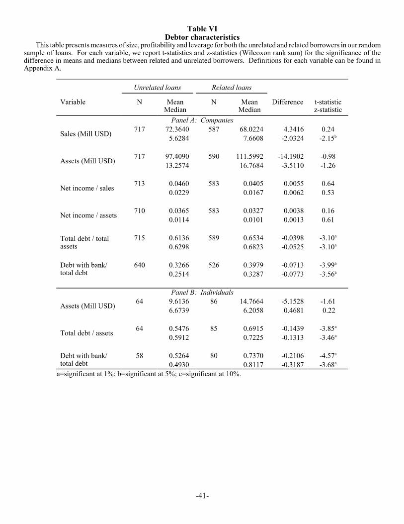
-41-

Table VIDebtor characteristics

This table presents measures of size, profitability and leverage for both the unrelated and related borrowers in our randomsample of loans. For each variable, we report t-statistics and z-statistics (Wilcoxon rank sum) for the significance of thedifference in means and medians between related and unrelated borrowers. Definitions for each variable can be found inAppendix A.

Unrelated loans Related loans

Variable N MeanMedian

N MeanMedian

Difference t-statisticz-statistic

Panel A: Companies

Sales (Mill USD) 717 72.3640 587 68.0224 4.3416 0.245.6284 7.6608 -2.0324 -2.15b

Assets (Mill USD) 717 97.4090 590 111.5992 -14.1902 -0.9813.2574 16.7684 -3.5110 -1.26

Net income / sales 713 0.0460 583 0.0405 0.0055 0.640.0229 0.0167 0.0062 0.53

Net income / assets 710 0.0365 583 0.0327 0.0038 0.160.0114 0.0101 0.0013 0.61

Total debt / totalassets

715 0.6136 589 0.6534 -0.0398 -3.10a

0.6298 0.6823 -0.0525 -3.10a

Debt with bank/total debt

640 0.3266 526 0.3979 -0.0713 -3.99a

0.2514 0.3287 -0.0773 -3.56a

Panel B: Individuals

Assets (Mill USD) 64 9.6136 86 14.7664 -5.1528 -1.616.6739 6.2058 0.4681 0.22

Total debt / assets 64 0.5476 85 0.6915 -0.1439 -3.85a

0.5912 0.7225 -0.1313 -3.46a

Debt with bank/total debt

58 0.5264 80 0.7370 -0.2106 -4.57a

0.4930 0.8117 -0.3187 -3.68a

a=significant at 1%; b=significant at 5%; c=significant at 10%.

-42-

Table VII - Panel ALoan terms regressions

OLS and Probit regressions for the cross-section of loans. For the probit, derivatives are calculated based on the averageof the scale factor in the case of the continuous regressors, and as the average of the difference in the cumulative normaldistributions evaluated with and without the dummy variable in the case of binomial regressors. Standard errors are shownin parenthesis. OLS regressions have robust standard errors. Definitions for each variable can be found in Appendix A.

Dependent variables:

Interest rates Collateral

Independentvariables:

Real interest rates Interest rate spreads Collateral dummy(Probit)

Collateral value /loan

(Tobit)

Related -0.0422a

(0.0039)-0.0415a

(0.0036)-0.0515a

(0.0040)-0.0515a

(0.0037)-0.2797a

(0.0268)-0.2992a

(0.0250)-2.9474a

(0.2749)-2.9842a

(0.2477)

Log of sales -0.0050a

(0.0012)-0.0033a

(0.0011)-0.0368a

(0.0075)-0.2252a

(0.0705)

Log of assets -0.0061a

(0.0012)-0.0040a

(0.0011)-0.0358a

(0.0084)-0.2372a

(0.0754)

Net income / sales -0.0016(0.0097)

-0.0035(0.0101)

-0.0493(0.0715)

-0.9010(0.6512)

Total debt / totalassets

0.0045(0.0099)

0.0015(0.0090)

-0.0076(0.0093)

0.0100(0.0085)

0.0557(0.0599)

0.0158(0.0568)

1.4546a

(0.5789)1.7421a

(0.5262)

Domestic currencydummy

-0.0600a

(0.0054)-0.0564a

(0.0041)-0.0292a

(0.0040)-0.0309a

(0.0038)-0.0419(0.0296)

-0.0612b

(0.0278)-0.3811(0.2877)

-0.3994(0.2599)

Fixed interest ratedummy

-0.0407a

(0.0054)-0.0422a

(0.0048)-0.0360a

(0.0057)-0.0385a

(0.0052)-0.2396a

(0.0320)-0.2318a

(0.0299)-1.3987a

(0.3121)-1.3471a

(0.2795)

Individual dummy 0.0042(0.0052)

0.0065(0.0054)

-0.0798c

(0.0429)-0.6483c

(0.3816)

Constant 0.1834a

(0.0287)0.2035a

(0.0283)0.1035a

(0.0305)0.1166a

(0.0304)5.4295a

(1.8122)5.6623a

(1.7884)

Bank dummies Yes Yes Yes Yes Yes Yes Yes YesLoan year dummies Yes Yes Yes Yes Yes Yes Yes YesIndustry dummies Yes Yes Yes Yes Yes Yes Yes Yes

Number ofobservations

1307 1470 1307 1470 1257 1418 1289 1451

Adjusted R2 /Pseudo R2

0.28 0.29 0.24 0.25 0.20 0.20 0.04 0.05

Log - likelihood -629.86 -707.40 -2842.09 -3145.93

a=significant at 1%; b=significant at 5%; c=significant at 10%.

-43-

Table VII - Panel BLoan terms regressions

Probit and Tobit regressions for the cross-section of loans. For the probit, derivatives are calculated based on the averageof the scale factor in the case of the continuous regressors, and as the average of the difference in the cumulative normaldistributions evaluated with and without the dummy variable in the case of binomial regressors. Standard errors are shownin parenthesis. Definitions for each variable can be found in Appendix A.

Dependent variables:

Independentvariables:

Personal guarantees(Probit)

Maturity in months(Tobit)

Grace period in months(Tobit)

Related -0.1918a

(0.0288)-0.2286a

(0.0277)7.2484a

(2.4564)6.0365b

(2.3681)20.9650a

(1.7933)20.2374a

(1.6612)

Log of sales -0.0117(0.0076)

-2.5309a

(0.6361)-1.3417b

(0.4533)

Log of assets -0.0280a

(0.0089)-1.3380c

(0.7214)-1.0094b

(0.5033)

Net income / sales -0.0224(0.0729)

10.0093c

(5.8785)6.9071c

(4.0067)

Total debt / totalassets

0.1584b

(0.0630)0.0413

(0.0620)-10.0349c

(5.2601)-13.5593a

(5.1138)-5.6744(3.7215)

-6.4817c

(3.4959)

Domestic currencydummy

-0.0661b

(0.0303)-0.0638b

(0.0299)2.1445

(2.5962)2.7273

(2.5095)0.2294

(1.8583)-0.0459(1.7268)

Fixed interest ratedummy

0.0569c

(0.0323)0.0416

(0.0317)-27.5106a

(2.7449)-27.9162a

(2.6349)-16.8188a

(2.0947)-16.4636a

(1.9197)

Individual dummy -0.3719a

(0.0399)-7.7577b

(3.7026)-9.6037a

(2.5244)

Constant 61.4569a

(16.7883)58.4428a

(17.6659)-0.1143

(11.4898)-2.6504

(11.6765)

Bank dummies Yes Yes Yes Yes Yes YesLoan year dummies Yes Yes Yes Yes Yes YesIndustry dummies Yes Yes Yes Yes Yes Yes

Number ofobservations

1307 1470 1307 1470 1307 1470

Adjusted R2 /Pseudo R2

0.09 0.13 0.02 0.02 0.06 0.05

Log - likelihood -790.33 -870.20 -6736.25 -7608.91 -2768.26 -3121.96

a=significant at 1%; b=significant at 5%; c=significant at 10%.

-44-

Table VIIILoan performance for the sample of unrelated and related loans

This table presents data on the incidence of non-performing loans in the random sample of loans. In Panel B, “other loanoutcomes” include: (1) bad loans that were later fully or partially liquidated without requiring court or internal collection;(2) loans for which required reserve was applied and the bank assumed a complete loss; and (3) loans for which negotiationsbetween the bank and the borrower are still undergoing. N is the number of loans in each category. The table reports t-statistics for differences in means. Definitions for each variable can be found in Appendix A.

Unrelated loans Related loans

N Frequency N Frequency Difference t-statPanel A: Performance of the loans

Loans that defaulted 317 0.3695 451 0.6642 -0.2947 -11.99a

Other bad loans 15 0.0175 24 0.0353 -0.0178 -2.21b

All bad loans 332 0.3869 475 0.6996 -0.3127 -12.81a

Panel B: Breakup of bad loans by outcome Restructured 44 0.1325 59 0.1242 0.0083 0.35Sold to FOBAPROA 10 0.0301 19 0.0400 -0.0099 -0.74Sent to court 205 0.6175 256 0.5389 0.0786 2.22b

Sent to collection department 35 0.1054 72 0.1516 -0.0462 -1.03Other loan outcomes 38 0.1145 69 0.1453 -0.0308 -1.27

a=significant at 1%; b=significant at 5%; c=significant at 10%.

-45-

Table IXRecovery rates for the sample of unrelated and related bad loans

This table presents data on the recovery rate of non-performing loans in the random sample of loans. N is the numberof loans in each category. The table reports t-statistics and z-statistics for differences in means and medians, respectively.Definitions for each variable can be found in Appendix A.

Unrelated loans Related loans

N Mean Median

N Mean Median

Difference t-statisticz-statistic

Panel A: All bad loansAll bad loans 332 0.4624 475 0.2721 0.1903 7.62a

0.4475 0.1500 0.2975 6.49a

All bad loans & no collateral 53 0.4206 204 0.2580 0.1626 3.08a

0.4299 0.1000 0.3299 2.14b

All bad loans & collateral<median 95 0.3705 315 0.2694 0.1011 2.52b

0.1800 0.1200 0.0600 1.56

Panel B: All loans

All loans 858 0.7920 679 0.4908 0.3012 15.07a

1.0000 0.4000 0.6000 13.94a

a=significant at 1%; b=significant at 5%; c=significant at 10%.

-46-

Table XLoan performance regressions

Probit and Tobit regressions of the cross-section of loans. For the probit, derivatives are calculated based on the averageof the scale factor in the case of the continuous regressors, and as the average of the difference in the cumulative normaldistributions evaluated with and without the dummy variable in the case of binomial regressors. Standard errors are shownin parenthesis. Definitions for each variable can be found in Appendix A.

Dependent variables:

Default Recovery rates

Independent variables: All bad loans(Probits)

All bad loans (Tobits)

All loans(Tobits)

Related 0.3303a

(0.0315)0.3509a

(0.0287)-0.2768a

(0.0461)-0.2840a

(0.0429)-0.6991a

(0.0664)-0.7796a

(0.0635)

Log of sales -0.0572a

(0.0096)0.0170

(0.0132)0.0919a

(0.0176)

Log of assets -0.0466a

(0.0100)0.0263c

(0.0155)0.0874a

(0.0199)

Net income / sales -0.6273a

(0.0933)0.1403

(0.1154)1.0442a

(0.1594)

Total debt / total assets 0.1833b

(0.0732)0.2884a

(0.0678)-0.0484(0.0994)

-0.0227(0.0932)

-0.2301c

(0.1380)-0.4537a

(0.1327)

Domestic currencydummy

0.0788b

(0.0360)0.0482

(0.0331)0.1691a

(0.0503)0.1229a

(0.0462)0.0048

(0.0685)-0.0167(0.0645)

Fixed interest ratedummy

0.0434(0.0379)

0.0445b

(0.0345)-0.0329(0.0515)

-0.0443(0.0472)

-0.0883(0.0703)

-0.1075(0.0662)

Individual dummy 0.1328a

(0.0470)-0.1058c

(0.0579)-0.2742a

(0.0878)

Constant 0.4317b

(0.2075)0.3817c

(0.2331)0.6188b

(0.2883)0.9430a

(0.3146)

Bank dummies Yes Yes Yes Yes Yes YesYear of loan dummies Yes Yes Yes Yes Yes YesIndustry dummies Yes Yes Yes Yes Yes Yes

Number of observations 1307 1470 665 791 1307 1470Log-likelihood -629.10 -730.70 -523.07 -620.48 -993.69 -1174.78Adjusted R2 / Pseudo R2 0.31 0.28 0.16 0.15 0.23 0.22

a=significant at 1%; b=significant at 5%; c=significant at 10%.

-47-

Table XIPublicly-traded debtor regressions

OLS, Probit and Tobit regressions of the cross-section of loans. For the probit, derivatives are calculated based on theaverage of the scale factor in the case of the continuous regressors, and as the average of the difference in the cumulativenormal distributions evaluated with and without the dummy variable in the case of binomial regressors. OLS regressions haverobust standard errors. Definitions for each variable can be found in Appendix A.

Dependent variables:

Interest rates Collateral Default Performance

Independent variables: Realinterest

rates

Interest ratespreads

Collateraldummy(Probit)

Collateral /loan

(Tobit)

All badloans

(Probit)

Recoveryrate

(Tobit)

Related -0.0450a

(0.0039)-0.0547a

(0.0040)-0.3295a

(0.0268)-3.1174a

(0.2653)0.4064a

(0.0301)-0.8442a

(0.0656)

Publicly traded -0.0339a

(0.0098)-0.0198b

(0.0089)-0.3069a

(0.0671)-1.6776a

(0.5277)-0.0955(0.0710)

0.2570(0.1731)

Publicly traded andrelated

0.0302a

(0.0118)0.0248a

(0.0105)0.1838a

(0.0425)1.4215b

(0.7051)-0.2943a

(0.0808)0.5209b

(0.2072)

Individual dummy 0.0031(0.0052)

0.0004(0.0054)

-0.0895b

(0.0436)-0.7141c

(0.3818)0.1131b

(0.0484)-0.2177a

(0.0861)

Log of assets -0.0048a

(0.0013)-0.0034a

(0.0012)-0.0237a

(0.0087)-0.1738b

(0.0779)-0.0361a

(0.0102)0.0634a

(0.0200)

Total debt / total assets -0.0037(0.0089)

-0.0087(0.0084)

-0.0017(0.0570)

-1.6537a

(0.5255)0.2994a

(0.0683)-0.4528b

(0.1295)

Domestic currencydummy

-0.0574a

(0.0041)-0.0314a

(0.0038)-0.0713b

(0.0278)-0.4517c

(0.2298)0.0429

(0.0337)0.0322

(0.0632)

Fixed interest ratedummy

-0.0417a

(0.0048)-0.0381a

(0.0051)-0.2289a

(0.0301)-1.3169a

(0.2791)0.0392

(0.0352)-0.0971a

(0.0648)

Constant 0.1933a

(0.0281)0.1103a

(0.0301)5.1223a

(1.7938)1.0783a

(03096)

Bank dummies Yes Yes Yes Yes Yes YesYear of loan dummies Yes Yes Yes Yes Yes YesIndustry dummies Yes Yes Yes Yes Yes Yes

Number of observations 1470 1470 1418 1451 1470 1470Adjusted R2 / Pseudo R2 0.30 0.25 0.21 0.05 0.30 0.23Log - likelihood -697.08 -3140.80 -708.75 -1152.98

a=significant at 1%; b=significant at 5%; c=significant at 10%.

-48-

Appendix ADescription of the variables

This table describes the quantitative variables collected for the terms and performance of a random sample of loans madeby 19 Mexican banks circa 1995. The banks in the sample are the 19 banks that existed in 1992 when privatization wasconcluded. With the exception of Citibank, all of them had recently been privatized. Reporting requirements in 1995 requiredbanks to submit a list of the largest three hundred loans together with their size and the names of the borrowers behind eachof them. The first column gives the name of the variable or the ratio. The second column describes the item. Sources: SAM-300 database (largest 300 loans for each bank), SENICREB database (complete list of loans made by each of the privatizedbanks), and every bank individual database reported for Mexican Banking Commission’s request.

Variable Description

Related loans According to the article 73 of the Mexican Code of Mercantile Institutions, a related loan is a loan for whichthe borrower is either: (1) a shareholder of 1% or more of the voting rights of the bank; (2) a person who hasfamily ties—by marriage or blood up to the second degree—with a shareholder of 1% or more of the votingrights of the bank; (3) a director, officer, or employee of a company or trust fund that holds 1% or more of thevoting rights of the bank or a director, officer, or employee of the bank itself with the power to engage intocontracts or transactions under the name bank; or (4) a person holding 10% or more of the voting rights of acompany that holds 1% or more of the shares in the bank.

Unrelated loan An unrelated loan is an arms-length loan given to a borrower who is not a shareholder, director, officer, oremployee of the bank nor a relative of any of the previous groups of persons.

Shareholder Any person or company holding, directly or indirectly, 1% or more of the voting shares of the financial groupor of the bank itself. Similarly, the definition of shareholder includes any person holding 10% or more of theshares of the borrowing company. For the purposes of Table 1, a shareholder can be either a holder of thebank’s equity or of a company’s that is related with the bank.

Director/Officer All members of the board of directors, officers, and employees of a borrowing company or of the bank itselfwith the power to engage into contracts or transactions under the name of the borrowing company or of thebank. This definition is in line with the statutes described in article 73 of the Mexican Code of MercantileInstitutions.

Family Any relative of shareholders, directors/officers, or employees of a borrowing company or the lending bankitself, related by either marriage or by blood up to the second degree.

Publicly traded Dummy variable that takes a value equal to 1 if the borrowing company was listed and publicly traded in theMexican Stock Exchange during the year of 1995; the variable takes a value equal to 0 otherwise.

Fixed interest-ratedummy

Dummy variable that takes a value equal to 1 if the loan pays a fixed interest rate; the variable takes a valueequal to 0 otherwise. A fixed interest rate loan pays an annual percentage rate on a fixed basis without beingupdated during the duration of the loan.

Flexible interest-ratedummy

Dummy variable that takes a value equal to 1 if the loan pays a flexible interest rate; the variable takes a valueequal to 0 otherwise. A flexible interest rate loan pays a spread above a reference rate and is updated with afrequency pre-established in the contract between the bank and the borrower. Typically, flexible interest ratesare referenced to market interest rates such as Treasury bills (CETES), the average annual percentage cost ofdeposits within the banking system (CPP), or the interbank interest rates (TIIE or TIIP).

Real interest rate The average real interest rate paid during the duration of the loan. The average real interest rate is computed

as: , where i is the reference interest rate assigned to the loan, s is the spread above the1 111T

i st

tt

T ( )( )+ ++= π

interest rate and π the inflation rate. For loans in Mexican pesos the inflation rate was calculated using theProducer Price Index (INPP) excluding oil products. For loans in US dollars and other foreign currencies theinflation rate was calculated using the US Producer Price Index (PPI) of finished products.

Variable Description

-49-

Interest rate spread The average interest rate spread of the loan above the benchmark risk-free security rate. The average interest

rate spread is computed as: , where rf is the risk-free security rate and s is the spread agreed11T

i s rt tf

t

T

( )+ −=

in the contract between the bank and the borrower above the loan reference rate i. For loans in Mexican pesosthe risk-free security is the 28-day Treasury bills (CETES) rate. For loans in US dollars and other foreigncurrencies, the risk-free security rate is the 1-month LIBOR rate.

Collateral Dummy that takes a value equal to 1 if the loan is backed up by collateral; the variable takes a value equal to0 otherwise. Definitions fro collateral include physical tangible assets, financial documents (e.g., titledocuments, securities, etc.), intangibles, and business proceeds pledged by the borrower to ensure repaymenton his loan. Collateral does not include personal guarantees such as obligations backed only by the signatureof the borrower or the submission of wealth statements from guarantors to the bank—a usual practice inMexico.

Personal guarantees Dummy that takes a value equal to 1 if the loan is secured by a personal guarantee; the variable takes a valueequal to 0 otherwise. A personal guarantee is defined as the obligation to repayment by a letter of compromise.Usually, the debtor must submit wealth statements from a guarantor who is willing to backs his loan.

Maturity The number of months to maturity of the loan starting from the moment in which the loan is given. Maturityvaries according to debtor characteristics, loan type, and terms established in the loan contract..

Months-to-maturityfrom 12/1994

The number of months for the loan to mature starting from December 1994. This variable is set to zero forall loans with a maturity date before or equal to December 1994.

Grace period Grace period is the number of months, beyond maturity, given to a debtor in order for him to repay his duebalance with the bank. A grace period is granted to a debtor on an individual basis. A loan may have no graceperiod at all but, if granted, the grace period may vary according to the loan type and terms established in theloan contract.

Net income / sales The ratio of net income to sales. Net income is equal to operating income minus interest expenses and nettaxes paid, as well as the cost of any extraordinary items. Sales are equal to the total value of products andservices sold, nationally and internationally, minus sales returns and discounts. Net income and sales figuresare from 1989-1998 (the first pair available) in millions of Mexican pesos that were deflated to December1995 using Mexico’s Producer Price Index and then converted to US dollars using the average 1995 exchangerate.

Sales (Mill USD) Sales in millions of US dollars deflated to December 1995. Sales are equal to the total value of products andservices sold, nationally and internationally, minus sales returns and discounts. Sales figures are from 1989-1998 (the first available) that were deflated to December 1995 using Mexico’s Producer Price Index and thenconverted to US dollars using the average 1995 exchange rate.

Log (sales) The natural logarithm of sales as defined above.

Assets (Mill USD) Assets in millions of US dollars deflated to December 1995. Total assets are equal to the total value of currentassets, long term receivables, investment in unconsolidated subsidiaries, other investments, net property plantand equipment and other assets. Total assets figures are from 1989-1998 (the first available) that were deflatedto December 1995 using Mexico’s Producer Price Index and then converted to US dollars using the average1995 exchange rate.

Log (assets) The natural logarithm of total assets as defined above.

Net income/assets The ratio of net income to total assets. Net income is equal to operating income minus interest expenses andnet taxes paid, as well as the cost of any extraordinary items. Total assets are equal to the total value of currentassets, long term receivables, investment in unconsolidated subsidiaries, other investments, net property plantand equipment and other assets. Net income and total assets figures are from 1989-1998 (the first pairavailable) in millions of Mexican pesos that were deflated to December 1995 using Mexico’s Producer PriceIndex and then converted to US dollars using the average 1995 exchange rate.

Variable Description

-50-

Total debt/total assets The ratio of total debt to total assets. Total debt is equal to the sum of all interest bearing obligations of thedebtor plus all other liabilities. Total assets is equal to the total value of current assets, long term receivables,investment in unconsolidated subsidiaries, other investments, net property plant and equipment and otherassets. Total debt and total assets figures are from 1989-1998 (the first pair available) in millions of Mexicanpesos that were deflated to December 1995 using Mexico’s Producer Price Index and then converted to USdollars using the average 1995 exchange rate.

Debt with bank/totaldebt

The ratio fo total bank debt to total debt. Debt with bank includes all outstanding loans that the debtor hadat the end of the first year it started relations with that bank. Total debt is equal to the sum of all interestbearing obligations of the debtor plus all other liabilities. Debt with the bank and total debt figures are from1989-1998 (the first pair available) in millions of Mexican pesos that were deflated to December 1995 usingMexico’s Producer Price Index and then converted to US dollars using the average 1995 exchange rate.

Domestic currencydummy

Dummy variable that takes a value equal to 1 if the currency is domestic, that is, Mexican pesos or theinflation-adjusted currency units UDIs (Unidad de Inversión); the variable takes a value equal to 0 otherwise.

Individual dummy Dummy variable that takes a value equal to 1 if the debtor is an individual—not a firm; the variable takes avalue equal to 0 otherwise.

Year of loandummies

Six fixed-year effect dummy variables. We generated a year of origination dummy variable for the years of1990, 1991, 1992, 1993, 1994, 1995, and 1996. The year of loan dummy takes the value equal to 1if loan wasoriginated in that year; the variable takes a value equal to 0 otherwise. The year of origination of the loan isthe year when the loan was contracted and granted.

Industry dummies Twelve industry dummy variables. We classified every debtor in one of 12 broad sectors of the economy. Thefollowing are the industries captured: (1) agriculture, fishery, and forestry; (2) minning; (3) manufacture offood, beverages, and tobacco; (4) construction; (5) electricity, gas, and water; (6) commerce, hotels, andrestaurants; (7) transportation; (8) financial services; (9) community services; (10) civil and mercantileassociations; (11) government, defense, public security; and (12) foreign and international organizations.

Non-performing loanorLoans that defaulted

A non-performing loan is a loan that has stopped payment on principal and interest and has defaulted on theoriginal terms of the borrower’s loan agreement at the moment we drew the sample of random loans. InMexico, the general rule for the classification of a loan as non-performing is the is that the debtor must missone coupon payment or as soon as it fails to pay interest payment when principal is payed at the end, whateverhappens first.

Other bad loans Other bad loans are defined as loans that were not non-performing but still were sent to Fobaproa or had arecovery rate of less than 100%.

All bad loans Total bad loans is the sum of other bad loans and non-performing loans. Total bad loans are the loans that:(1) were non-performing; or (2) were sold to Fobaproa; or (3) had recovery rates of less than 100%.

Loans sold toFOBAPROA

A loan sold to Fobaproa is a non-performing loan sold to the deposit insurance agency Fobaproa (Fondo deProtección al Ahorro Bancario).

Restructured loans A restructured loan is a loan for which the original terms have been altered due to the deterioration of thedebtor’s financial condition. A restructure is generally undertaken in order to avoid complete default oruncollectibility from the debtor. In most of the cases, a restructure involves the extension of the maturity ofthe loan, the change of the interest rate terms, and/or the rescheduling of payments.

Loans sent to court A loan sent to court is a non-performing loan for which the bank initiated a judicial proceeding (generally civillawsuit) against the debtor in a Mexican court of law in order to recover the debtor’s due balance with thebank, by either taking over the assets put forward as guarantee or achieving a court injunction favorable to thebank..

Variable Description

-51-

Loans sent toadministrativecollection

A loan sent to administrative collection is a non-performing loan for which the bank filed an internal paymentcollection procedure. The procedure works on a borrower-by-borrower basis and is intended to make theborrower resume payments on her defaulted loan, either by negotiating a restructure, a forgiveness of her debt,or both. This is procedure functions as a warning for the borrower with due payments and is less stringent thana court procedure. Generally, if administrative collection fails the bank will then file a lawsuit against thedebtor in a Mexican court of law.

Other loan outcomes Other loan outcomes include: (1) bad loans that were later fully or partially liquidated without requiring courtor internal collection; (2) loans for which required reserve was applied and the bank assumed a complete loss;and (3) loans for which negotiations between the bank and the borrower are still undergoing.

Collateralized loans A collateralized loan is a loan for which an asset has been pledged by the debtor in order to ensure repaymenton the face value of the loan. Our definition of collateral includes physical assets, financial documents (e.g.,title documents), intangibles, and business proceeds pledged by the borrower to ensure repayment, but rulesout personal guarantees such as obligations backed only by the signature of the debtor or guarantors.