LOCA on Tehran by RELAP5-MOD3.2 Code 1-s2.0-S0149197007000704-Main
RELAP5/MOD3.3 CODE MANUALVOLUME I:
CODE STRUCTURE,SYSTEM MODELS, AND SOLUTION METHODS
Nuclear Safety Analysis Division
December 2001Information Systems Laboratories, Inc.
Rockville, MarylandIdaho Falls, Idaho
Prepared for the Division of Systems Research
Office of Nuclear Regulatory ResearchU. S. Nuclear Regulatory Commission
Washington, DC 20555
1

2

ABSTRACT
The RELAP5/MOD3.3 code has been developed for best-estimate transient simulation of light water
reactor coolant systems during postulated accidents. The code models the coupled behavior of the reactor
coolant system and the core for loss-of-coolant accidents and operational transients such as anticipated
transient without scram, loss of offsite power, loss of feedwater, and loss of flow. A generic modeling
approach is used that permits simulating a variety of thermal hydraulic systems. Control system and
secondary system components are included to permit modeling of plant controls, turbines, condensers, and
secondary feedwater systems.
RELAP5/MOD3.3 code documentation is divided into seven volumes: Volume 1 presents modeling
theory and associated numerical schemes; Volume 2 details instructions for code application and input data
preparation; Volume 3 presents the results of developmental assessment cases that demonstrate and verify
the models used in the code; Volume 4 discusses in detail RELAP5 models and correlations; Volume 5
presents guidelines that have evolved over the past several years through the use of the RELAP5 code;
Volume 6 discusses the numerical scheme used in RELAP5; Volume 7 presents a collection of
independent assessment calculations; and Volume 8 contains information of interest to RELAP5
programmers.
3 NUREG/CR-5535/Rev 1-Vol I

NUREG/CR-5535/Rev 1-Vol I 4
CONTENTS
Page
1 INTRODUCTION.........................................................................................................................1
1.1 Development of RELAP5/MOD3.3 .................................................................................1
1.1.1 References ...........................................................................................................3
1.2 Relationship to Previous Code Versions...........................................................................3
1.2.1 References ...........................................................................................................4
1.3 Quality Assurance ............................................................................................................4
2 CODE ARCHITECTURE.............................................................................................................5
2.1 Computer Adaptability .....................................................................................................5
2.2 Top Level Organization ....................................................................................................5
2.3 Input Processing Overview...............................................................................................6
2.4 Transient Overview ..........................................................................................................7
3 HYDRODYNAMIC MODEL..................................................................................................... 11
3.0.1 References .........................................................................................................12
3.1 Field Equations...............................................................................................................15
3.1.1 Basic Differential Equations .............................................................................153.1.2 Numerically Convenient Set of Differential Equations ....................................333.1.3 Semi-Implicit Scheme Difference Equations ....................................................363.1.4 Time Advancement for the Semi-Implicit Scheme ...........................................463.1.5 Difference Equations and Time Advancement for the
Nearly-Implicit Scheme ....................................................................................553.1.6 Volume-Average Velocities ...............................................................................633.1.7 Implicit Hydrodynamic and Heat Structure Coupling ......................................693.1.8 Numerical Solution of Boron Transport Equation ............................................723.1.9 References .........................................................................................................75
3.2 State Relationships .........................................................................................................79
3.2.1 State Equations ..................................................................................................793.2.2 Single-Component, Two-Phase Mixture ...........................................................803.2.3 Two-Component, Two-Phase Mixture ..............................................................843.2.4 References .........................................................................................................92
3.3 Constitutive Models........................................................................................................93
3.3.1 Vertical Volume Flow Regime Map ..................................................................943.3.2 Horizontal Volume Flow Regime Map .............................................................993.3.3 High Mixing Volume Flow Regime Map........................................................1013.3.4 ECC Mixer Volume Flow Regime Map ..........................................................1013.3.5 Junction Flow Regime Map ............................................................................1053.3.6 Interphase Friction...........................................................................................1073.3.7 Coefficient of Virtual Mass .............................................................................1313.3.8 Wall Friction....................................................................................................132
5 NUREG/CR-5535/Rev 1-Vol I

3.3.9 Wall Heat Transfer Models..............................................................................1413.3.10 Wall Heat Transfer Correlations......................................................................1453.3.11 Interphase Mass Transfer ................................................................................1483.3.12 Direct Heating .................................................................................................1653.3.13 References .......................................................................................................165
3.4 Special Process Models ................................................................................................171
3.4.1 Choked Flow ...................................................................................................1713.4.2 Horizontal Stratification Entrainment/Pullthrough Model..............................1843.4.3 Abrupt Area Change........................................................................................1863.4.4 User-Specified Form Loss...............................................................................1963.4.5 Crossflow Junction ..........................................................................................1973.4.6 Water Packing Mitigation Scheme ..................................................................2013.4.7 Countercurrent Flow Limitation Model ..........................................................2033.4.8 Mixture Level Tracking Model .......................................................................2073.4.9 Thermal Stratification Model ..........................................................................2253.4.10 Energy Conservation at an Abrupt Change .....................................................2333.4.11 Jet Junction Model...........................................................................................2343.4.12 References .......................................................................................................234
3.5 Component Models ......................................................................................................239
3.5.1 Branch .............................................................................................................2393.5.2 Separator..........................................................................................................2423.5.3 Jet Mixer..........................................................................................................2543.5.4 Pump................................................................................................................2613.5.5 Turbine ............................................................................................................2733.5.6 Valves ..............................................................................................................2803.5.7 Accumulator ....................................................................................................2933.5.8 ECC Mixer ......................................................................................................3093.5.9 Annulus ...........................................................................................................3263.5.10 References .......................................................................................................326
4 HEAT STRUCTURE MODELS ...............................................................................................329
4.1 Heat Conduction Numerical Techniques......................................................................329
4.2 Mesh Point and Thermal Property Layout ...................................................................330
4.3 Difference Approximation at Internal Mesh Points .....................................................333
4.4 Difference Approximation at Boundaries ....................................................................335
4.5 Thermal Properties and Boundary Condition Parameters ............................................336
4.6 RELAP5 Specific Boundary Conditions .....................................................................337
4.6.1 Correlation Package Conditions......................................................................3374.6.2 Insulated and Tabular Boundary Conditions ...................................................340
4.7 Solution of Simultaneous Equations ............................................................................340
4.8 Computation of Heat Fluxes.........................................................................................342
4.9 Two-Dimensional Conduction Solution/Reflood .........................................................343
4.10 Fine Mesh Rezoning Scheme .......................................................................................347
NUREG/CR-5535/Rev 1-Vol I 6

4.10.1 References .......................................................................................................349
4.11 Gap Conductance Model ..............................................................................................349
4.11.1 References .......................................................................................................358
4.12 Surface-to-Surface Radiation Model ............................................................................358
4.12.1 References .......................................................................................................360
4.13 Metal-Water Reaction Model .......................................................................................361
4.13.1 References .......................................................................................................362
4.14 Cladding Deformation Model.......................................................................................362
4.14.1 References .......................................................................................................368
5 TRIP SYSTEM..........................................................................................................................369
5.1 Variable Trips ...............................................................................................................369
5.2 Logical Trips.................................................................................................................369
6 CONTROL SYSTEM................................................................................................................371
6.1 Arithmetic Control Components ..................................................................................371
6.1.1 Constant...........................................................................................................3716.1.2 Addition-Subtraction .......................................................................................3716.1.3 Multiplication ..................................................................................................3716.1.4 Division ...........................................................................................................3716.1.5 Exponentiation.................................................................................................3726.1.6 Table Lookup Function ...................................................................................3726.1.7 Standard Functions ..........................................................................................3726.1.8 Delay ...............................................................................................................3726.1.9 Unit Trip ..........................................................................................................3726.1.10 Trip Delay........................................................................................................373
6.2 Integration Control Component....................................................................................373
6.3 Differentiation Control Components ............................................................................374
6.4 Proportional-Integral Component.................................................................................375
6.5 Lag Control Component ...............................................................................................376
6.6 Lead-Lag Control Component......................................................................................377
6.7 Shaft Component ..........................................................................................................378
7 POINT REACTOR KINETICS MODEL .................................................................................381
7.1 Point Reactor Kinetics Equations.................................................................................381
7.2 Fission Product Decay Model ......................................................................................382
7.3 Actinide Decay Model..................................................................................................385
7.4 Transformation of Equations for Solution....................................................................386
7.5 Initialization..................................................................................................................388
7.6 Reactivity Feedback .....................................................................................................389
7 NUREG/CR-5535/Rev 1-Vol I
7.6.1 Separable Feedback Model .............................................................................3897.6.2 Tabular Feedback Model .................................................................................3907.6.3 Reference.........................................................................................................396
7.7 Reactor Kinetics Numerical Procedures.......................................................................396
7.7.1 References .......................................................................................................400
8 SPECIAL TECHNIQUES.........................................................................................................401
8.1 Time Step Control ........................................................................................................401
8.1.1 New Mass/Energy Cell-Based (Material) Courant Limit................................4018.1.2 Momentum Cell-Based (Momentum) Courant Limit .....................................4038.1.3 Original Material Courant Limit .....................................................................4058.1.4 Mass Error Check............................................................................................4058.1.5 Other Checks ...................................................................................................407
8.2 Mass/Energy Error Mitigation......................................................................................408
8.3 Steady-State..................................................................................................................409
8.3.1 Fundamental Concepts for Detecting Hydrodynamic Steady-State During Transient Calculations ...................................................409
8.3.2 Calculational Precision and the Steady-State Convergence Criteria...............4138.3.3 Steady-State Testing Scheme, Time Interval Control, and Output..................4178.3.4 Heat Structure Heat Conductance Scheme for Steady-State...........................4208.3.5 Interrelationship of Steady-State and Transient Restart/Plot Records ............421
8.4 Self-Initialization..........................................................................................................421
8.4.1 General Description.........................................................................................4218.4.2 Required Plant Model Characteristics .............................................................4228.4.3 Standard Suboptions........................................................................................4238.4.4 Inherent Model Incompatibilities ....................................................................4258.4.5 Description of Standard Controllers................................................................425
NUREG/CR-5535/Rev 1-Vol I 8

FIGURES
Page2.2-1 RELAP5 top level structure........................................................................................................... 62.4-1 Modular structures of transient calculations in RELAP5.............................................................. 82.4-2 Transient/steady-state block structure ........................................................................................... 83.1-1 Interface heat transfer in the bulk and near the wall for subcooled boiling ................................ 213.1-2 Relation of central angle to void fraction ................................................................................... 303.1-3 Difference equation nodalization schematic................................................................................ 383.1-4 Schematic of a volume cell showing multiple inlet and outlet junction mass flows................... 633.3-1 Schematic of Vertical Flow Regime Map with Hatchings Indicating Transitions ...................... 953.3-2 Schematic of Horizontal Flow Regime Map with Hatchings Indicating Transition Regions ... 1003.3-3 Schematic of High Mixing Volume Flow Regime Map ............................................................ 1023.3-4 Schematic of ECC Mixer Volume Flow Regime Map (modified Tandon et al.) ...................... 1033.3-5 Slug Flow Pattern ...................................................................................................................... 1233.3-6 Three Vertical Volumes with the Middle Volume Being Vertically Stratified........................... 1263.3-7 Flow Regimes Before and After the Critical Heat Flux (CHF) Transition ............................... 1313.3-8 RELAP5 Boiling and Condensing Curves ................................................................................ 1433.3-9 RELAP5 Wall Heat Transfer Flow Chart .................................................................................. 1443.4-1 Equilibrium Speed of Sound as a Function of Void Fraction and Virtual Mass Coefficient..... 1763.4-2 Coefficient of Relative Mach Number for Thermal Equilibrium Flow as a Function of
Void Fraction and Virtual Mass Coefficient .............................................................................. 1773.4-3 Subcooled Choking Process ...................................................................................................... 1783.4-4 Pressure Distribution for Choked Flow Through a Converging-Diverging Nozzle.................. 1833.4-5 Abrupt Expansion ...................................................................................................................... 1883.4-6 Abrupt Contraction .................................................................................................................... 1893.4-7 Orifice at Abrupt Area Change.................................................................................................. 1903.4-8 Schematic Flow of Two-Phase Mixture at Abrupt Area Change .............................................. 1933.4-9 Modeling of Crossflows or Leak ............................................................................................... 1993.4-10 Simplified Tee Crossflow .......................................................................................................... 2003.4-11 Leak Flow Modeling ................................................................................................................. 2013.4-12 Two Vertical Vapor/Liquid Volumes ......................................................................................... 2033.4-13 Pressure-Drop Characteristics Near the Boundary Between Countercurrent and
Cocurrent Flow .......................................................................................................................... 2043.4-14 Plot of versus for a Typical CCFL Correlation........................................................................ 2053.4-15 Mixture Level in Normal Void Profile ...................................................................................... 2093.4-16 Mixture Level in a Volume Below a Void Fraction Inversion................................................... 2093.4-17 Mixture Level Above a Void Fraction Inversion....................................................................... 2103.4-18 Level Detection Logic Diagram ................................................................................................ 2123.4-19 Level Detection Logic for Volume L Above an Inverted Profile .............................................. 2133.4-20 Level Detection Logic Diagram for Volume L Below an Inverted Profile ............................... 2143.4-21 Level Detection Logic Diagram for a Normal Profile............................................................... 2153.4-22 The Control Volume for Momentum Cell j ............................................................................... 2233.4-23 Hydrodynamic Volume with Heat Structure ............................................................................. 2253.4-24 Thermal Front in a Tank ............................................................................................................ 2273.4-25 Thermal Front Detection Logic Diagram for Volume L............................................................ 228
9 NUREG/CR-5535/Rev 1-Vol I
3.4-26 Computation of Thermal Front Parameters Logic Diagram for Volume L ............................... 2313.4-27 Hydrodynamic Volume with Thermal Front ............................................................................. 2333.5-1 One-Dimensional Branch .......................................................................................................... 2403.5-2 Gravity Effects on a Tee ............................................................................................................ 2423.5-3 Typical Separator Volume and Junctions................................................................................... 2433.5-4 Donor Junction Voids for Outflow ............................................................................................ 2443.5-5 Schematic of First Stage of Mechanistic Separator................................................................... 2453.5-6 Dryer Capacity........................................................................................................................... 2553.5-7 Schematic of Mixing Junctions ................................................................................................. 2563.5-8 Flow Regimes and Dividing Streamline.................................................................................... 2603.5-9 Typical Pump Characteristic Four-Quadrant Curves................................................................. 2643.5-10 Typical Pump Homologous Head Curves ................................................................................. 2653.5-11 Typical Pump Homologous Torque Curves............................................................................... 2663.5-12 Single-Phase Homologous Head Curves for 1-1/2 Loop MOD1 Semiscale Pumps................. 2673.5-13 Fully Degraded, Two-phase Homologous Head Curves for 1-1/2 Loop MOD1
Semiscale Pumps ....................................................................................................................... 2683.5-14 Torque versus Speed, Type 93a Pump Motor (Rated Voltage).................................................. 2723.5-15 A Schematic of a Stage Group with Idealized Flow Path between Points 1 and 2 ................... 2743.5-16 Schematic of Lumped Model for Turbine Stage Group ............................................................ 2803.5-17 Diagram of Inertial Valve .......................................................................................................... 2843.5-18 Two Views of a Partially Open Flapper Valve .......................................................................... 2853.5-19 Schematic of a Typical Relief Valve in the Closed Position ..................................................... 2873.5-20 Schematic of a Typical Relief Valve in the Partially Open Position ......................................... 2883.5-21 Schematic of a Typical Relief Valve in the Fully Open Position .............................................. 2893.5-22 Typical Cylindrical Accumulator .............................................................................................. 2943.5-23 Typical Spherical Accumulator ................................................................................................. 2953.5-24 ECCMIX Component ................................................................................................................ 3103.5-25 Schematic Cross-Section of Stratified Flow Along the ECCMIX Component,
Showing the Length of Interface (Lm) and the Jet Length (Ljet) ............................................... 3133.5-26 Schematic Vertical Cross-Section of the ECCMIX Component, Showing the
Width of Liquid Surface, Ls, and the Tending Half-Angle........................................................ 3144.2-2 Typical Mesh Points .................................................................................................................. 3314.2-1 Mesh Point Layout..................................................................................................................... 3314.2-3 Boundary Mesh Points............................................................................................................... 3324.9-1 Volume and Surface Elements Around a Mesh Point (i, j)........................................................ 3444.10-1 An Elementary Heat Structure Unit for Reflood ....................................................................... 3484.10-2 An Example of the fine Mesh-Rezoning Process...................................................................... 3494.11-1 Segmentation at the Fuel-Cladding Gap.................................................................................... 3504.14-1 ORNL Correlation of Rupture Temperature as a Function of Engineering Hoop
Stress and Temperature-Ramp Rate with Data from Internally Heated Zircaloy Cladding in Aqueous Atmospheres ........................................................................................... 364
4.14-2 Maximum Circumferential Strain as a Function of Rupture Temperature for Internally Heated Zircaloy Cladding in Aqueous Atmospheres at Heating Rates Less Than or Equal to 10 C/s..................................................................................................... 367
4.14-3 Maximum Circumferential Strain as a Function of Rupture Temperature for Internally Heated Zircaloy Cladding in Aqueous Atmospheres at Heating Rates Greater Than or Equal to 25 C/s................................................................................................ 367
NUREG/CR-5535/Rev 1-Vol I 10

4.14-4 Reduction in PWR Assembly Flow Area as a Function of Rupture Temperature and Ramp... 3688.1-1 Difference Equation Nodalization Schematic ........................................................................... 403
11 NUREG/CR-5535/Rev 1-Vol I

NUREG/CR-5535/Rev 1-Vol I 12
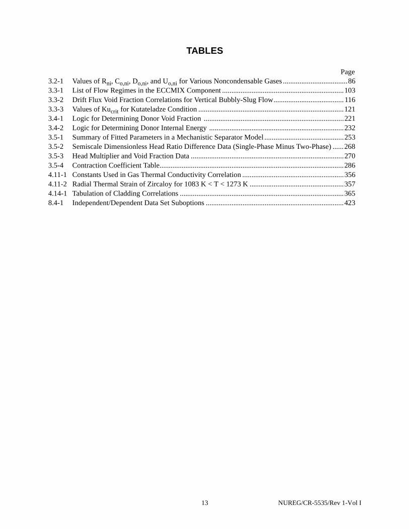
TABLES
Page3.2-1 Values of Rni, Co,ni, Do,ni, and Uo,ni for Various Noncondensable Gases ...................................863.3-1 List of Flow Regimes in the ECCMIX Component ..................................................................1033.3-2 Drift Flux Void Fraction Correlations for Vertical Bubbly-Slug Flow...................................... 1163.3-3 Values of Kucrit for Kutateladze Condition ...............................................................................1213.4-1 Logic for Determining Donor Void Fraction ............................................................................2213.4-2 Logic for Determining Donor Internal Energy .........................................................................2323.5-1 Summary of Fitted Parameters in a Mechanistic Separator Model ...........................................2533.5-2 Semiscale Dimensionless Head Ratio Difference Data (Single-Phase Minus Two-Phase) ......2683.5-3 Head Multiplier and Void Fraction Data ...................................................................................2703.5-4 Contraction Coefficient Table....................................................................................................2864.11-1 Constants Used in Gas Thermal Conductivity Correlation .......................................................3564.11-2 Radial Thermal Strain of Zircaloy for 1083 K < T < 1273 K ...................................................3574.14-1 Tabulation of Cladding Correlations .........................................................................................3658.4-1 Independent/Dependent Data Set Suboptions ...........................................................................423
13 NUREG/CR-5535/Rev 1-Vol I

NUREG/CR-5535/Rev 1-Vol I 14
EXECUTIVE SUMMARY
The light water reactor (LWR) transient analysis code, RELAP5, was developed at the Idaho
National Engineering Laboratory (INEL) for the U.S. Nuclear Regulatory Commission (NRC). Code uses
include analyses required to support rulemaking, licensing audit calculations, evaluation of accident
mitigation strategies, evaluation of operator guidelines, and experiment planning analysis. RELAP5 has
also been used as the basis for a nuclear plant analyzer. Specific applications have included simulations of
transients in LWR systems such as loss of coolant, anticipated transients without scram (ATWS), and
operational transients such as loss of feedwater, loss of offsite power, station blackout, and turbine trip.
RELAP5 is a highly generic code that, in addition to calculating the behavior of a reactor coolant system
during a transient, can be used for simulation of a wide variety of hydraulic and thermal transients in both
nuclear and nonnuclear systems involving mixtures of steam, water, noncondensable, and solute.
RELAP5/MOD3.3 has been developed jointly by the NRC and a consortium consisting of several
countries and domestic organizations that were members of the International Code Assessment and
Applications Program (ICAP) and its successor organization, Code Applications and Maintenance
Program (CAMP). Credit also needs to be given to various Department of Energy sponsors, including the
INEL laboratory-directed discretionary funding program. The mission of the RELAP5/MOD3.3
development program was to develop a code version suitable for the analysis of all transients and
postulated accidents in LWR systems, including both large- and small-break loss-of-coolant accidents
(LOCAs) as well as the full range of operational transients.
The RELAP5/MOD3.3 code is based on a nonhomogeneous and nonequilibrium model for the two-
phase system that is solved by a fast, partially implicit numerical scheme to permit economical calculation
of system transients. The objective of the RELAP5 development effort from the outset was to produce a
code that included important first-order effects necessary for accurate prediction of system transients but
that was sufficiently simple and cost effective so that parametric or sensitivity studies were possible.
The code includes many generic component models from which general systems can be simulated.
The component models include pumps, valves, pipes, heat releasing or absorbing structures, reactor point
kinetics, electric heaters, jet pumps, turbines, separators, accumulators, and control system components. In
addition, special process models are included for effects such as form loss, flow at an abrupt area change,
branching, choked flow, boron tracking, and noncondensable gas transport.
The system mathematical models are coupled into an efficient code structure. The code includes
extensive input checking capability to help the user discover input errors and inconsistencies. Also
included are free-format input, restart, renodalization, and variable output edit features. These user
conveniences were developed in recognition that generally the major cost associated with the use of a
system transient code is in the engineering labor and time involved in accumulating system data and
developing system models, while the computer cost associated with generation of the final result is usually
small.
15 NUREG/CR-5535/Rev 1-Vol I

The development of the models and code versions that constitute RELAP5 has spanned more than 20
years from the early stages of RELAP5 numerical scheme development to the present. RELAP5 represents
the aggregate accumulation of experience in modeling reactor core behavior during accidents, two-phase
flow processes, and LWR systems. The code development has benefited from extensive application and
comparison to experimental data in the LOFT, PBF, Semiscale, ACRR, NRU, and other experimental
programs.
Several new models, improvements to existing models, and user conveniences have been added to
RELAP5/MOD3.3. The new models include
• The Bankoff counter-current flow limiting correlation that can be activated by the user at
each junction in the system model.
• The ECCMIX component for modeling of the mixing of subcooled emergency core
cooling system (ECCS) liquid and the resulting interfacial condensation.
• A zirconium-water reaction model to model the exothermic energy production on the
surface of zirconium cladding material at high temperature.
• A surface-to-surface radiation heat transfer model with multiple thermal radiation
enclosures defined through user input.
• A level tracking model.
• A thermal stratification model.
• A new thermodynamically consistent set of steam tables for light water based on the
International Association for the Properties of Water and Steam (IAPWS) Formulation
1995 for the Thermodynamic Properties of Ordinary Water Substance for General and
Scientific Use.
• CANDU models.
Improvements to existing models include
• New correlations for interfacial friction for all types of geometry in the bubbly-slug flow
regime in vertical flow passages.
• Use of junction-based interphase drag.
• An improved model for vapor pullthrough and liquid entrainment in horizontal pipes to
obtain correct computation of the fluid state convected through a break.
NUREG/CR-5535/Rev 1-Vol I 16

• A new critical heat flux correlation for rod bundles based on tabular data.
• An improved horizontal stratification inception criterion for predicting the flow regime
transition between horizontally stratified and dispersed flow.
• A modified reflood heat transfer model.
• Improved logic for vertical stratification inception to avoid excessive activation of the
water packing model.
• An improved boron transport model.
• A mechanistic separator/dryer model.
• An improved crossflow model.
• An improved form loss model.
• The addition of a simple plastic strain model with a clad burst criterion to the fuel
mechanical model.
• The addition of a radiation heat transfer term to the gap conductance model.
• Modifications to the noncondensable gas model to eliminate erratic code behavior and
failure.
• Improvements to the downcomer penetration, ECCS bypass, and upper plenum
deentrainment capabilities.
• Henry-Fauske and Moody choking models.
Additional user and programmer conveniences include
• Computer portability through the conversion of the FORTRAN coding to adhere to the
FORTRAN 77 standard.
• Code execution and validation on a variety of systems. The code should be easily installed
(i.e., the installation script is supplied with the transmittal) on the CRAY X-MP
(UNICOS), DECstation 5000 (ULTRIX), DEC Alpha Workstation (OSF/1), IBM
Workstation 6000 (UNIX), SUN Workstation (UNIX), SGI Workstation (UNIX), and HP
Workstation (UNIX), Linux Workstations, both little and big Endian computers, and
Windows (NT, 9x, 2000). The code can be installed easily on all 64-bit machines (integer
17 NUREG/CR-5535/Rev 1-Vol I

and floating point operands) and any 32-bit machine that provides for 64-bit floating
point.
• Removal of the bit-packing.
The RELAP5/MOD3.3 code manual consists of eight separate volumes and one appendix to Volume
II. The modeling theory and associated numerical schemes are described in Volume I, to acquaint the user
with the modeling base and thus aid in effective use of the code. Volume II contains more detailed
instructions for code application. The Appendix to Volume II contains specific instructions for input data
preparation. Both Volumes I and II are expanded and revised versions of the RELAP5/MOD2 code
manuala and Volumes I and III of the SCDAP/RELAP5/MOD2 code manual.b
Volume III presents the results of developmental assessment cases run with RELAP5/MOD3.3 to
demonstrate and validate the models used in the code. The assessment matrix contains phenomenological
problems, separate-effects tests, and integral systems tests.
Volume IV contains a detailed discussion of the models and correlations used in RELAP5/MOD3.3.
It presents the user with the underlying assumptions and simplifications used to generate and implement
the base equations into the code so that an intelligent assessment of the applicability and accuracy of the
resulting calculations can be made. Thus, the user can determine whether RELAP5/MOD3.3 is capable of
modeling his or her particular application, whether the calculated results will be directly comparable to
measurement or whether they must be interpreted in an average sense, and whether the results can be used
to make quantitative decisions.
Volume V provides guidelines for users that have evolved over the past several years from
applications of the RELAP5 code at the Idaho National Engineering Laboratory, at other national
laboratories, and by users throughout the world.
Volume VI discusses the numerical scheme in RELAP5/MOD3.3, and Volume VII is a collection of
independent assessment calculations.
Volume VIII provides information of interest to RELAP5/MOD3.3 programmers.
a. V. H. Ransom, et al. RELAP5/MOD2 Code Manual, Volumes I and II. NUREG/CR-4312, EGG-2396. Idaho
National Engineering Laboratory. August 1995 and December 1985, revised March 1987.
b. C. M. Allison and E. C. Johnson, Eds. SCDAP/RELAP5/MOD2 Code Manual, Volume I: RELAP5 Code
Structure, System Models, and Solution Methods, and Volume III: User’s Guide and Input Requirements.
NUREG/CR-5273, EGG-2555. Idaho National Engineering Laboratory. June 1989.
NUREG/CR-5535/Rev 1-Vol I 18

ACKNOWLEDGMENTS
Development of a complex computer code such as RELAP5/MOD3.3 is the result of team effort and
requires the diverse talents of a large number of people. Special acknowledgment is given to those who
pioneered and continue to contribute to the RELAP5 code, in particular, V. H. Ransom, J. A. Trapp, and
R. J. Wagner. A number of other people have made and continue to make significant contributions to the
continuing development of the RELAP5 code. Recognition and gratitude is given to the members of the
INEL RELAP5 team:
V. T. Berta C. E. Lenglade R. A. Riemke
K. E. Carlson M. A. Lintner R. R. Schultz
C. D. Fletcher C. C. McKenzie A. S-L. Shieh
E. E. Jenkins G. L. Mesina R. W. Shumway
E. C. Johnsen C. S. Miller C. E. Slater
G. W. Johnsen G. A. Mortensen S. M. Sloan
J. M. Kelly P. E. Murray M. Warnick
H-H. Kuo R. B. Nielson W. L. Weaver
N. S. Larson S. Paik G. E. Wilson
The list of contributors is incomplete, as many others have made significant contributions in the past.
Rather than attempt to list them all and risk unknowingly omitting some who have contributed, we
acknowledge them as a group and express our appreciation for their contributions to the success of the
RELAP5 effort.
The list of contributors to the RELAP5 Program at SCIENTECH, Inc., include:
Bill Arcieri Doug Barber Robert Beaton
Robert Copp Byron Hansen Scott Lucas
Glen Mortensen Dan Prelewicz Rex Shumway
Randy Tompot Weidong Wang
The list of contributors to the RELAP5 Program at Information Systems Laboratories, Inc., include:
Bill Arcieri Doug Barber Robert Beaton
Mark Bolander Glen Mortensen Don Fletcher
Dan Prelewicz Rex Shumway Randy Tompot
The RELAP5 Program is indebted to the technical monitors from the U. S. Nuclear Regulatory
Commission and the Department of Energy-Idaho Operations Office for giving direction and management
to the overall program. Those from the NRC include W. Lyon, Y. Chen, R. Lee, R. Landry, H. Scott,
M. Rubin, D. E. Solberg, D. Ebert, S. Smith, T. Lee, V. Mousseau, Weidong Wang, Jennifer Uhle, and F.
19 NUREG/CR-5535/Rev 1-Vol I
Eltawila. Monitors from DOE-ID when the RELAP5 program was at the INEL include N. Bonicelli, C.
Noble, W. Rettig, and D. Majumdar.
The technical editing of the RELAP5 manuals when the RELAP5 program was at the INEL was
done by D. Pack and E. May.
Finally, acknowledgment is made of all the code users who have been very helpful in stimulating
timely correction of code deficiencies and suggesting improvements.
NUREG/CR-5535/Rev 1-Vol I 20

NOMENCLATURE
A cross-sectional area (m2), coefficient matrix in hydrodynamics, coefficient inpressure and velocity equations
A1 coefficient in heat conduction equation at boundaries
At throat area (m2)
a speed of sound (m/s), interfacial area per unit volume (m-1), coefficient in gapconductance, coefficient in heat conduction equation, absorption coefficient
B coefficient matrix, drag coefficient, coefficient in pressure and velocity equations
B1 coefficient in heat conduction equation at boundaries
b coefficient in heat conduction equation, source vector in hydrodynamics
Bx body force in x coordinate direction (m/s2)
By body force in y coordinate direction (m/s2)
C coefficient of virtual mass, general vector function, coefficient in pressure andvelocity equations, delayed neutron precursors in reactor kinetics, concentration,pressure-dependent coefficient in Unal’s correlation (1/K•s)
Co coefficient in noncondensable energy equation (J/kg•K)
C0, C1 constants in drift flux model
CD drag coefficient
Cp specific heat at constant pressure (J/kg•K)
Cv specific heat at constant volume (J/kg•K), valve flow coefficient
c coefficient in heat conduction equation, coefficient in new-time volume-averagevelocity equation, constant in CCFL model
D coefficient of relative Mach number, diffusivity, pipe diameter or equivalentdiameter (hydraulic diameter) (m), heat conduction boundary condition matrix,coefficient in pressure and velocity equations
Do coefficient in noncondensable energy equation (J/kg•K2)
D1 coefficient of heat conduction equation at boundaries
d coefficient in heat conduction equation, droplet diameter (m)
DISS energy dissipation function (W/m3)
E total energy (U + v2/2) (J/kg), emissivity, Young’s modulus, term in iterative heatconduction algorithm, coefficient in pressure equation
e interfacial roughness
F term in iterative heat conduction algorithm, gray-body factor with subscript,frictional loss coefficient, vertical stratification factor
21 NUREG/CR-5535/Rev 1-Vol I

FA force per unit volume
FIF, FIG interphase drag coefficients (liquid, vapor) (s-1)
FI interphase drag coefficient (m3/kg•s)
FWF, FWG wall drag coefficients (liquid, vapor) (s-1)
f interphase friction factor, vector for liquid velocities in hydrodynamics
G mass flux (kg/m2-s), shear stress, gradient, coefficient in heat conduction, vectorquantity, fraction of delayed neutrons in reactor kinetics
GC dynamic pressure for valve (Pa)
Gr Grashof number
g gravitational constant (m/s2), temperature jump distance (m), vector for vaporvelocities in hydrodynamics
H elevation (m), volumetric heat transfer coefficient (W/K•m3), head (m)
HLOSSF, HLOSSG form or frictional losses (liquid, vapor) (m/s)
h specific enthalpy (J/kg), heat transfer coefficient (W/m2•K), energy transfercoefficient for Γg, head ratio
hL dynamic head loss (m)
I identity matrix, moment of inertia (N-m-s2)
J junction velocity (m/s)
j superficial velocity
K energy form loss coefficient
Ks Spring constant
Ku Kutateladze number
k thermal conductivity (W/m•K)
kB Boltzmann constant
L length, limit function, Laplace capillary length
M Mach number, molecular weight, pump two-phase multiplier, mass transfer rate,mass (kg)
m constant in CCFL model
N number of system nodes, number density (#/m3), pump speed (rad/s),nondimensional number
Nu Nusselt number
n unit vector, order of equation system
PBP valve closing back pressure (Pa)
NUREG/CR-5535/Rev 1-Vol I 22
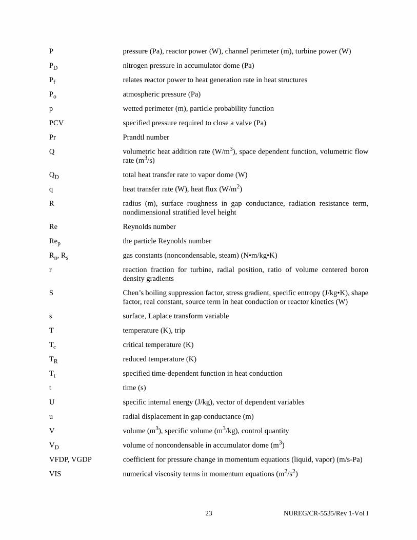
P pressure (Pa), reactor power (W), channel perimeter (m), turbine power (W)
PD nitrogen pressure in accumulator dome (Pa)
Pf relates reactor power to heat generation rate in heat structures
Po atmospheric pressure (Pa)
p wetted perimeter (m), particle probability function
PCV specified pressure required to close a valve (Pa)
Pr Prandtl number
Q volumetric heat addition rate (W/m3), space dependent function, volumetric flowrate (m3/s)
QD total heat transfer rate to vapor dome (W)
q heat transfer rate (W), heat flux (W/m2)
R radius (m), surface roughness in gap conductance, radiation resistance term,nondimensional stratified level height
Re Reynolds number
Rep the particle Reynolds number
Rn, Rs gas constants (noncondensable, steam) (N•m/kg•K)
r reaction fraction for turbine, radial position, ratio of volume centered borondensity gradients
S Chen’s boiling suppression factor, stress gradient, specific entropy (J/kg•K), shapefactor, real constant, source term in heat conduction or reactor kinetics (W)
s surface, Laplace transform variable
T temperature (K), trip
Tc critical temperature (K)
TR reduced temperature (K)
Tt specified time-dependent function in heat conduction
t time (s)
U specific internal energy (J/kg), vector of dependent variables
u radial displacement in gap conductance (m)
V volume (m3), specific volume (m3/kg), control quantity
VD volume of noncondensable in accumulator dome (m3)
VFDP, VGDP coefficient for pressure change in momentum equations (liquid, vapor) (m/s-Pa)
VIS numerical viscosity terms in momentum equations (m2/s2)
23 NUREG/CR-5535/Rev 1-Vol I

VISF, VISG numerical viscosity terms in momentum equations (liquid, vapor) (m2/s2)
VUNDER, VOVER separator model parameters (liquid, vapor)
v mixture velocity (m/s), phasic velocity (m/s), flow ratio, liquid surge line velocity(m/s)
vc choking velocity (m/s)
W weight of valve disk, weighting function in reactor kinetics, relaxation parameterin heat conduction, shaft work per unit mass flow rate, mass flow rate
Wcrit critical Weber number
We Weber number
w humidity ratio
X flow quality, static quality, mass fraction, conversion from MeV/s to watts
x spatial coordinate (m), vector of hydrodynamic variables
Y control variable
Z two-phase friction correlation factor, function in reactor kinetics
∆Z height of volume
z elevation change coordinate (m)
Symbols
α void fraction, subscripted volume fraction, angular acceleration (rad/s2),coefficient for least-squares fit, speed ratio
β coefficient of isobaric thermal expansion (K-1), effective delayed neutron fractionin reactor kinetics
Γ volumetric mass exchange rate (kg/m3•s)
γ exponential function in decay heat model
∆Pf dynamic pressure loss (Pa)
∆Ps increment in steam pressure (Pa)
∆Vs increment in specific volume of steam (m3/kg)
∆t increment in time variable (s)
∆tc Courant time step (s)
∆x increment in spatial variable (m)
δ area ratio, truncation error measure, film thickness (m), impulse function,Deryagin number
ε coefficient, strain function, emissivity, tabular function of area ratio, surfaceroughness, wall vapor generation/condensation flag
NUREG/CR-5535/Rev 1-Vol I 24

ζ diffusion coefficient, multiplier, or horizontal stratification terms
η efficiency, bulk/saturation enthalpy flag
θ relaxation time in correlation for Γ, angular position (rad), discontinuity detectorfunction
κ coefficient of isothermal compressibility (Pa-1)
Λ prompt neutron generation time, Baroczy dimensionless property index
λ eigenvalue, interface velocity parameter, friction factor, decay constant in reactorkinetics
µ viscosity (kg/m•s)
ν kinematic viscosity (m2/s), Poisson’s ratio
ξ exponential function, RMS precision
π 3.141592654
ρ density (kg/m3), reactivity in reactor kinetics (dollars)
∑f fission cross-section
∑′ depressurization rate (Pa/s)
σ surface tension (J/m2), stress, flag used in heat conduction equations to indicatetransient or steady-state
τ shear stresses (N), torque (N-m)
υ specific volume (m3/kg)
φ donored property, Lockhart-Martinelli two-phase parameter, neutron flux inreactor kinetics, angle of inclination of valve assembly, velocity-dependentcoefficient in Unal’s correlation
Φ Roe’s superbee gradient limiter
χ Lockhart-Martinelli function
ψ coefficient, fission rate (number/s)
ω angular velocity, constant in Gudanov solution scheme
Subscripts
AM annular mist to mist flow regime transition
a average value
ann liquid film in annular mist flow regime
BS bubbly-to-slug flow regime transition
b bubble, boron
25 NUREG/CR-5535/Rev 1-Vol I

bulk bulk fluid
CHF value at critical heat flux condition
c vena contracta, continuous phase, cladding, critical property, cross-section,condensation
cm cladding midpoint
co carryover
core vapor core in annular-mist flow regime
cr, crit critical property or condition
cu carryunder
D drive line, vapor dome, discharge passage of mechanical separator
DE value at lower end of slug to annular-mist flow regime transition
d droplet, delay in control component
drp droplet
e equilibrium, equivalent quality in hydraulic volumes, value ring exit, elasticdeformation, entrainment
ent entrainment
F wall friction, fuel
FB, FBB film boiling, Bromley film boiling
f liquid phase, flooding, film, flow
fg phasic difference (i.e., vapor term-liquid term)
flow flow
fp onset of vapor pull-through
fr frictional
front value at thermal stratification front
g vapor phase, gap
ge incipient liquid entrainment
H head
HE homogeneous equilibrium
h, hy, hydro hydraulic
I interface
IAN inverted annular flow regime
i interface, index
NUREG/CR-5535/Rev 1-Vol I 26

in volume inlets
iso isothermal
j, j+1, j-1 spatial noding indices for junctions
K spatial noding index for volumes
k iteration index in choking model
L spatial noding index for volume, laminar
lev, level value at two-phase level
l left boundary in heat conduction
M rightmost boundary in heat conduction, spatial noding index for volume
m mixture property, motor, mesh point
min minimum value
NOZ nozzle
n noncondensable component of vapor phase
o reference value
out volume outlets
p partial pressure of steam, particle, projected
pipe cross-section of flow channel
R rated values
r relative Mach number, right boundary in heat structure mesh
ref reference value
rms root mean square
S suction region
SA value at upper end of slug to annular-mist flow regime transition
s steam component of vapor phase, superheated
sat saturated quality
sb small bubbles
sr surface of heat structure
st stratified
std standard precision
T point of minimum area, turbulent
TB transition boiling
27 NUREG/CR-5535/Rev 1-Vol I

Tb Taylor bubble
t total pressure, turbulent, tangential, throat
up upstream quantity
v mass mean Mach number, vapor quantity, valve
w wall, water
wall wall
wg, wf wall to vapor, wall to liquid
1 upstream station, multiple junction index, vector index
1φ single-phase value
2 downstream station, multiple junction index, vector index
2φ two-phase value
τ torque
µ viscosity
infinity
~ vector
≈ Matrix
Superscripts
B bulk liquid
b boundary gradient weight factor in heat conduction, vector quantities
exp old time terms in velocity equation, used to indicate explicit velocities in choking
m-1, m, m+1 mesh points in heat conduction finite difference equation or mean value
n, n+l time level index
n+1/2 an average of quantities with superscripts n and n+1
o initial value
R real part of complex number, right boundary in heat conduction
s saturation property, space gradient weight factor in heat conduction
v volume gradient weight factor in heat conduction
W wall
1 vector index, coefficient in velocity equation
2 vector index
∞
NUREG/CR-5535/Rev 1-Vol I 28
* total derivative of a saturation property with respect to pressure, local variable,bulk/saturation property
′ derivative
- vector, average quantity
. donored quantity
~ unit momentum for mass exchange, intermediate time variable
linearized quantity, quality based on total mixture massˆ
29 NUREG/CR-5535/Rev 1-Vol I

NUREG/CR-5535/Rev 1-Vol I 30
INTRODUCTION
1 INTRODUCTION
The RELAP5 computer code is a light water reactor transient analysis code developed for the U.S.
Nuclear Regulatory Commission (NRC) for use in rulemaking, licensing audit calculations, evaluation of
operator guidelines, and as a basis for a nuclear plant analyzer. Specific applications of this capability have
included simulations of transients in LWR systems, such as loss of coolant, anticipated transients without
scram (ATWS), and operational transients such as loss of feedwater, loss of offsite power, station blackout,
and turbine trip. RELAP5 is a highly generic code that, in addition to calculating the behavior of a reactor
coolant system during a transient, can be used for simulation of a wide variety of hydraulic and thermal
transients in both nuclear and nonnuclear systems involving mixtures of steam, water, noncondensable,
and solute.
1.1 Development of RELAP5/MOD3.3
RELAP5/MOD3.3 has been developed jointly by the NRC and a consortium consisting of several
countries and domestic organizations that were members of the International Code Assessment and
Applications Program (ICAP) and its successor organization, Code Applications and Maintenance
Program (CAMP). In addition, improvements have been made on behalf of several Department of Energy
sponsors. The mission of the RELAP5/MOD3 development program was to develop a code version
suitable for the analysis of all transients and postulated accidents in LWR systems, including both large-
and small-break loss-of-coolant accidents (LOCAs) as well as the full range of operational transients.
RELAP5/MOD3 was produced by improving and extending the modeling base that was established
with the release of RELAP5/MOD21.1-1,1.1-2,1.1-3 in 1985. Code deficiencies identified by members of
ICAP and CAMP through assessment calculations were noted, prioritized, and subsequently addressed.
Consequently, several new models, improvements to existing models, and user conveniences have been
added to RELAP5/MOD3.3. The new models include
• The Bankoff counter-current flow limiting correlation, that can be activated by the userat each junction in the system model.
• The ECCMIX component for modeling of the mixing of subcooled emergency corecooling system (ECCS) liquid and the resulting interfacial condensation.
• A zirconium-water reaction model to model the exothermic energy production on thesurface of zirconium cladding material at high temperature.
• A surface-to-surface radiation heat transfer model with multiple radiation enclosuresdefined through user input.
• A level tracking model.
• A thermal stratification model.
1 NUREG/CR-5535/Rev 1-Vol I

INTRODUCTION
• A new thermodynamically consistent set of steam tables for light water based on theInternational Association for the Properties of Water and Steam (IAPWS) Formulation1995 for the Thermodynamic Properties of Ordinary Water Substance for General andScientific Use.
• CANDU models.
Improvements to existing models include
• New correlations for interfacial friction for all types of geometry in the bubbly-slug flowregime in vertical flow passages.
• Use of junction-based interphase drag.
• An improved model for vapor pullthrough and liquid entrainment in horizontal pipes toobtain correct computation of the fluid state convected through the break.
• A new critical heat flux correlation for rod bundles based on tabular data.
• An improved horizontal stratification inception criterion for predicting the flow regimetransition between horizontally stratified and dispersed flow.
• A modified reflood heat transfer model.
• Improved vertical stratification inception logic to avoid excessive activation of the waterpacking model.
• An improved boron transport model.
• A mechanistic separator/dryer model.
• An improved crossflow model.
• An improved form loss model.
• The addition of a simple plastic strain model with clad burst criterion to the fuelmechanical model.
• The addition of a radiation heat transfer term to the gap conductance model.
• Modifications to the noncondensable gas model to eliminate erratic code behavior andfailure.
• Improvements to the downcomer penetration, ECCS bypass, and upper plenumdeentrainment capabilities.
NUREG/CR-5535/Rev 1-Vol I 2

INTRODUCTION
• Henry-Fauske and Moody choking flow models.
Additional user conveniences include
• Computer portability through the conversion of the FORTRAN coding to adhere to theFORTRAN 77 standard and its extensions. It has even been compiled using the Fortran90 compiler on a few CPUs.
• Code execution and validation on a variety of systems. The code should be easilyinstalled (i.e., the installation script is supplied with the transmittal) on the CRAY, DECRISC, DEC ALPHA, DEC ALPHA F90, IBM RISC, SUN SOLARIS, SUN OS, SGI,SGI 64-BIT, STARDENT, HP, HP F90, VAX, LINUX BIG ENDIAN, LINUX LITTLEENDIAN, and WINDOWS PC The code should be able to be installed on all 64-bitmachines (integer and floating point operands) and any 32-bit machine that provides for64-bit floating point operations.
1.1.1 References
1.1-1. V. H. Ransom, et al. RELAP5/MOD2 Code Manual, Volumes 1 and 2. NUREG/CR-4312, EGG-2396. Idaho National Engineering Laboratory. August 1985 and December 1985, revised March1987.
1.1-2. V. H. Ransom, et al. RELAP5/MOD2 Code Manual, Volume 3: Developmental AssessmentProblems. EGG-TFM-7952. Idaho National Engineering Laboratory. December 1987.
1.1-3. R. A. Dimenna, et al. RELAP5/MOD2 Models and Correlations. NUREG/CR-5194, EGG-2531.Idaho National Engineering Laboratory. August 1988.
1.2 Relationship to Previous Code Versions
The series of RELAP codes began with RELAPSE (REactor Leak And Power Safety Excursion),
which was released in 1966. Subsequent versions of this code are RELAP2,1.2-1 RELAP3,1.2-2 and
RELAP4,1.2-3 in which the original name was shortened to Reactor Excursion and Leak Analysis Program
(RELAP). All of these codes were based on a homogeneous equilibrium model (HEM) of the two-phase
flow process. The last code version of this series is RELAP4/MOD7,1.2-4 which was released to the
National Energy Software Center (NESC) in 1980.
In 1976, the development of a nonhomogeneous, non equilibrium model was undertaken for
RELAP4. It soon became apparent that a total rewrite of the code was required to efficiently accomplish
this goal. The result of this effort was the beginning of the RELAP5 project.1.2-5 As the name implies, this
is the fifth in the series of computer codes that was designed to simulate the transient behavior of LWR
systems under a wide variety of postulated accident conditions. RELAP5 follows the naming tradition of
previous RELAP codes, i.e., the odd numbered series are complete rewrites of the program while the even
numbered versions had extensive model changes, but used the architecture of the previous code. Each
3 NUREG/CR-5535/Rev 1-Vol I
INTRODUCTION
version of the code reflects the increased knowledge and new simulation requirements from both large-
and small-scale experiments, theoretical research in two-phase flow, numerical solution methods,
computer programming advances, and the increased capability of computers.
The principal new feature of the RELAP5 series was the use of a two-fluid, nonequilibrium,
nonhomogeneous, hydrodynamic model for transient simulation of the two-phase system behavior.
RELAP5/MOD2 employed a full nonequilibrium, six-equation, two-fluid model. The use of the two-fluid
model eliminated the need for the RELAP4 submodels, such as the bubble rise and enthalpy transport
models, which were necessary to overcome the limitations of the single-fluid model.
1.2.1 References
1.2-1. K. V. Moore and W. H. Rettig. RELAP2 - A Digital Program for Reactor Blowdown and PowerExcursion Analysis. IDO-17263. Idaho National Engineering Laboratory. March 1968.
1.2-2. W. H. Rettig et al. RELAP3 - A Computer Program for Reactor Blowdown Analysis. IN-1445.Idaho National Engineering Laboratory. February 1971.
1.2-3. K. V. Moore and W. H. Rettig. RELAP4 - A Computer Program for Transient Thermal-HydraulicAnalysis. ANCR-1127. Idaho National Engineering Laboratory. March 1975.
1.2-4. S. R. Behling et al. RELAP4/MOD7 - A Best Estimate Computer Program to Calculate Thermaland Hydraulic Phenomena in a Nuclear Reactor or Related System. NUREG/CR-1988, EGG-2089. Idaho National Engineering Laboratory. August 1981.
1.2-5. V. H. Ransom et al. RELAP5/MOD1 Code Manual, Volumes 1 and 2. NUREG/CR-1826, EGG-2070. Idaho National Engineering Laboratory. March 1982.
1.3 Quality Assurance
RELAP5 is maintained under a strict code-configuration system that provides a historical record of
the changes in the code. Changes are made using a version control system that allows separate
identification of improvements made to each successive version of the code. Modifications and
improvements to the coding are reviewed and checked as part of a formal quality program for software. In
addition, the theory and implementation of code improvements are validated through assessment
calculations that compare the code-predicted results to idealized test cases or experimental results.
NUREG/CR-5535/Rev 1-Vol I 4

CODE ARCHITECTURE
2 CODE ARCHITECTURE
Modeling flexibility, user-convenience, computer efficiency, and design for future growth were
primary considerations in the selection of the basic architecture of the code. The following sections cover
computer adaptability, code top level organization, input processing, and transient operation.
2.1 Computer Adaptability
RELAP5/MOD3.3 is written in FORTRAN 77 for a variety of 64-bit and 32-bit computers. Here, a
64-bit computer is one in which floating point, integer, and logical quantities use 64-bit words; a 32-bit
machine uses 32-bit words for those same quantities but also allows 64-bit floating point operations.
Examples of 64-bit computers are Cray and SGI 64-BIT, and DEC Alpha workstations. Examples of 32-bit
computers include DEC, HP, IBM, SGI, and SUN workstations, and personal computers.
A common source is maintained for all computer versions. The common source is conditioned for a
particular computer and operating system through the use of two precompilers maintained as part of
RELAP5. The first precompiler processes compile time options such as machine and operating system
dependencies. Through the use of standard Fortran and a widely used standard for bit operations, there is
very little hardware dependence. The primary hardware dependence is in matrix factoring routines where
details of the floating point characteristics are needed to monitor roundoff error. The program has been
compiled and executed using Fortran-90; a future full conversion to that standard should remove all
hardware dependencies. RELAP5 is developed and maintained at ISL on computers using the UNIX
operating system. Some user-convenient features have been incorporated into the code based on UNIX, but
these are under a compile time option. The code does not depend on any particular operating system. The
installation scripts distributed with the code are UNIX based, and control language to install and execute
the code must be developed by the user for other operating systems. The source code appears to be written
only for 64-bit machines. The second precompiler, however, converts the code for 32-bit computers by
converting floating point variables to double precision, changing floating point literals to double precision,
and adding an additional subscript to integer and logical arrays that are equivalenced to double precision
floating point arrays such that they index as 64-bit quantities even though only 32-bit integer arithmetic
and logical operations are used. As an example of the additional subscript, an integer statement would be
changed from INTEGER IA(1000000) to INTEGER IA(2,1000000) on big Endian computers and to
INTEGER IA(1,1000000) on little Endian computers.
Transmittals of the code usually show the installation and execution of sample problems on several
machines. The machines used depend on the machines currently available to the development staff.
2.2 Top Level Organization
RELAP5 is coded in a modular fashion using top-down structuring. The various models and
procedures are isolated in separate subroutines. The top level structure is shown in Figure 2.2-1 and
consists of input (INPUT), transient/steady-state (TRNCTL), and stripping (STRIP) blocks.
5 NUREG/CR-5535/Rev 1-Vol I

CODE ARCHITECTURE
The input block (INPUT) processes input, checks input data, and prepares required data blocks for all
program options and is discussed in more detail in Section 2.3.
The transient/steady-state block (TRNCTL) handles both transient and the steady-state options. The
steady-state option determines the steady-state conditions if a properly posed steady-state problem is
presented. Steady-state is obtained by running an accelerated transient until the time derivatives approach
zero. Thus, the steady-state option is very similar to the transient option but contains convergence testing
algorithms to determine satisfactory steady-state, divergence from steady-state, or cyclic operation. If the
transient technique alone were used, approach to steady-state from an initial condition would be identical
to a plant transient from that initial condition. Pressures, densities, and flow distributions would adjust
quickly, but thermal effects would occur more slowly. To reduce the transient time required to reach
steady-state, the steady-state option artificially accelerates heat conduction by reducing the thermal
capacity of the conductors. The transient/steady-state block is discussed in more detail in Section 2.4.
The strip block (STRIP) extracts simulation data from a restart plot file for convenient passing of
RELAP5 simulation results to other computer programs.
2.3 Input Processing Overview
RELAP5 provides detailed input checking for all system models using three input processing phases.
The first phase reads all input data, checks for punctuation and typing errors (such as multiple decimal
points and letters in numerical fields), and stores the data keyed by card number such that the data are
easily retrieved. A list of the input data is provided, and punctuation errors are noted.
During the second phase, restart data from a previous simulation are read if the problem is a
RESTART type, and all input data are processed. Some processed input is stored in fixed common blocks,
but the majority of the data are stored in dynamic data (common) blocks that are created only if needed by
a problem and sized to the particular problem. In a NEW-type problem, dynamic blocks must be created.
In RESTART problems, dynamic blocks may be created, deleted, added to, partially deleted, or modified
as modeling features and components within models are added, deleted, or modified. Extensive input
checking is done, but at this level, checking is limited to new data from the cards being processed.
Relationships with other data cannot be checked because the latter may not yet be processed. As an
Figure 2.2-1 RELAP5 top level structure
RELAP5
INPUT TRNCTL STRIP
NUREG/CR-5535/Rev 1-Vol I 6
CODE ARCHITECTURE
illustration of this level of checking, junction data are checked to determine if they are within the
appropriate range (such as positive, nonzero, or between zero and one) and volume connection codes are
checked for proper format. No attempt is made at this point to check whether or not referenced volumes
exist in the problem until all input data are processed.
The third phase of processing begins after all input data have been processed. Since all data have
been placed in fixed common or dynamic data (common) blocks during the second phase, complete
checking of interrelationships can proceed. Examples of cross-checking are existence of hydrodynamic
volumes referenced in junctions and heat structure boundary conditions; entry or existence of material
property data specified in heat structures; and validity of variables selected for minor edits, plotting, or
used in trips and control systems. As the cross-checking proceeds, cross-linking of the data blocks is done
so that it need not be repeated at every time step. The initialization required to prepare the model for the
start of the transient advancement is done at this level.
Input data editing and diagnostic messages can be generated during the second and/or third phases.
Input processing for most models generates output and diagnostic messages during both phases. Thus,
input editing for these models appears in two sections.
As errors are detected, various recovery procedures are used so that input processing can be
continued and a maximum amount of diagnostic information can be furnished. Recovery procedures
include supplying default or benign data, marking the data as erroneous so that other models do not attempt
use of the data, or deleting the bad data. The recovery procedures sometimes generate additional diagnostic
messages. Often after attempted correction of input, different diagnostic messages appear. These can be
due to continued incorrect preparation of data, but the diagnostics may result from the more extensive
testing permitted as previous errors are eliminated.
2.4 Transient Overview
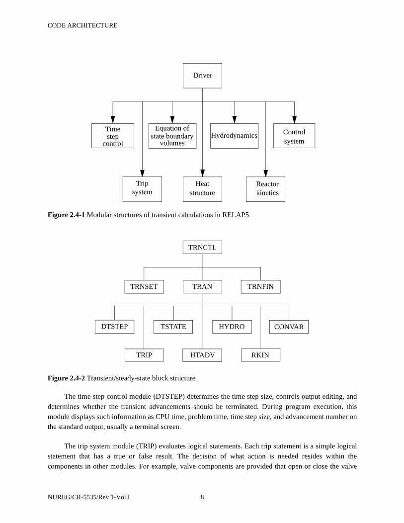
Figure 2.4-1 shows the functional modular structure for the transient calculations, while Figure 2.4-
2 shows the second-level structures for the transient/steady-state blocks or subroutines.
The subroutine TRNCTL shown in Figure 2.4-2 consists only of the logic to call the next lower level
routines. Subroutine TRNSET performs final cross-linking of information between data blocks, sets up
arrays to control the sparse matrix solution, establishes scratch work space, and returns unneeded computer
memory. Subroutine TRAN, the driver, controls the transient advancement of the solution. Nearly all the
execution time is spent in this block, and this block is the most demanding of memory. Nearly all the
dynamic data blocks must be in the central memory, and the memory required for instruction storage is
high, since coding to advance all models resides in this block. When transient advances are terminated, the
subroutine TRNFIN releases space for the dynamic data blocks that are no longer needed.
A description is next presented of the functions of all of the modules (subroutines) driven by TRAN
(see Figure 2.4-2).
7 NUREG/CR-5535/Rev 1-Vol I
CODE ARCHITECTURE
The time step control module (DTSTEP) determines the time step size, controls output editing, and
determines whether the transient advancements should be terminated. During program execution, this
module displays such information as CPU time, problem time, time step size, and advancement number on
the standard output, usually a terminal screen.
The trip system module (TRIP) evaluates logical statements. Each trip statement is a simple logical
statement that has a true or false result. The decision of what action is needed resides within the
components in other modules. For example, valve components are provided that open or close the valve
Figure 2.4-1 Modular structures of transient calculations in RELAP5
Figure 2.4-2 Transient/steady-state block structure
Driver
Timestep
control
Equation ofstate boundary
volumesHydrodynamics Control
system
Reactorkinetics
Heatstructure
Tripsystem
TRNCTL
TRNSET TRAN TRNFIN
DTSTEP TSTATE HYDRO CONVAR
TRIP HTADV RKIN
NUREG/CR-5535/Rev 1-Vol I 8

CODE ARCHITECTURE
based on trip values; pump components test trip status to determine whether a pump electrical breaker has
tripped.
The equation of state boundary volume module (TSTATE) calculates the thermodynamic state of the
fluid in each hydrodynamic boundary volume (time-dependent volume). This subroutine also computes
velocities for the time-dependent junctions.
The heat structure module (HTADV) advances heat conduction/transfer solutions. It calculates heat
transferred across solid boundaries of hydrodynamic volumes.
The hydrodynamics module (HYDRO) advances the hydrodynamic solution.
The reactor kinetics module (RKIN) advances the reactor kinetics of the code. It computes the power
behavior in a nuclear reactor using the space-independent or point kinetics approximation, which assumes
that power can be separated into space and time functions.
The control system module (CONVAR) provides the capability of simulating control systems
typically used in hydrodynamic systems. It consists of several types of control components. Each
component defines a control variable as a specific function of time-advanced quantities. The time-
advanced quantities include quantities from hydrodynamic volumes, junctions, pumps, valves, heat
structures, reactor kinetics, trip quantities, and the control variables themselves. This permits control
variables to be developed from components that perform simple, basic operations.
In the next sections of this volume of the manual, the various transient modules will be discussed.
These are in the following order: hydrodynamics, heat structures, trips, control system, reactor kinetics,
and special techniques (includes time step control).
9 NUREG/CR-5535/Rev 1-Vol I

CODE ARCHITECTURE
NUREG/CR-5535/Rev 1-Vol I 10

HYDRODYNAMIC MODEL
3 HYDRODYNAMIC MODEL
The RELAP5 hydrodynamic model is a one-dimensional, transient, two-fluid model for flow of a
two-phase steam-water mixture that can contain noncondensable components in the steam phase and/or a
soluble component in the water phase.
The RELAP5 hydrodynamic model contains several options for invoking simpler hydrodynamic
models. These include homogeneous flow, thermal equilibrium, and frictionless flow models. These
options can be used independently or in combination. The homogeneous and equilibrium models were
included primarily to be able to compare code results with calculations from the older codes based on the
homogeneous equilibrium model.
The two-fluid equations of motion that are used as the basis for the RELAP5 hydrodynamic model
are formulated in terms of volume and time-averaged parameters of the flow. Phenomena that depend upon
transverse gradients, such as friction and heat transfer, are formulated in terms of the bulk properties using
empirical transfer coefficient formulations. In situations where transverse gradients cannot be represented
within the framework of empirical transfer coefficients, such as subcooled boiling, additional models
specially developed for the particular situation are employed. The system model is solved numerically
using a semi-implicit finite-difference technique. The user can select an option for solving the system
model using a nearly-implicit finite-difference technique, which allows violation of the material Courant
limit. This option is suitable for steady-state calculations and for slowly varying, quasi-steady transient
calculations.
The basic two-fluid differential equations possess complex characteristic roots that give the system a
partially elliptic character and thus constitute an ill-posed initial boundary value problem. In RELAP5, the
numerical problem is rendered well-posed by the introduction of artificial viscosity terms in the difference
equation formulation that damp the high frequency spatial components of the solution. The ill-posed
character of the two-fluid model is a result of the spatial averaging process and neglect of higher-order
physical effects in the momentum formulation. Ransom and Hicks3.0-1 have studied several formulations
in which two pressures (one for each fluid) are included in the model, and these models are totally
hyperbolic and thus constitute well-posed problems. A curious feature of the two-pressure approach, that
was pointed out by Trapp and Ransom,a is that a well-posed problem is obtained without the addition of
any viscous effects, which are known to be responsible for physical stabilization in real flows. Trapp and
Ransoma indicated that in this case, a well-posed problem is obtained as a result of an unphysically large
transverse inertia at short wave lengths. In addition, the two-pressure model was developed for stratified
flows having a simple interfacial geometry, and it is unclear how to extend this concept to more general
interfacial geometries. Limited numerical studies by Ransom and Scofield3.0-2 have shown that solutions
for the two-pressure model compare very well to that for the single-pressure model with damping. In
general, the differences are significant only for short wavelength components of the solution where
a. Personal communication, J. A. Trapp and V. H. Ransom, January 1990.
11 NUREG/CR-5535/Rev 1-Vol I
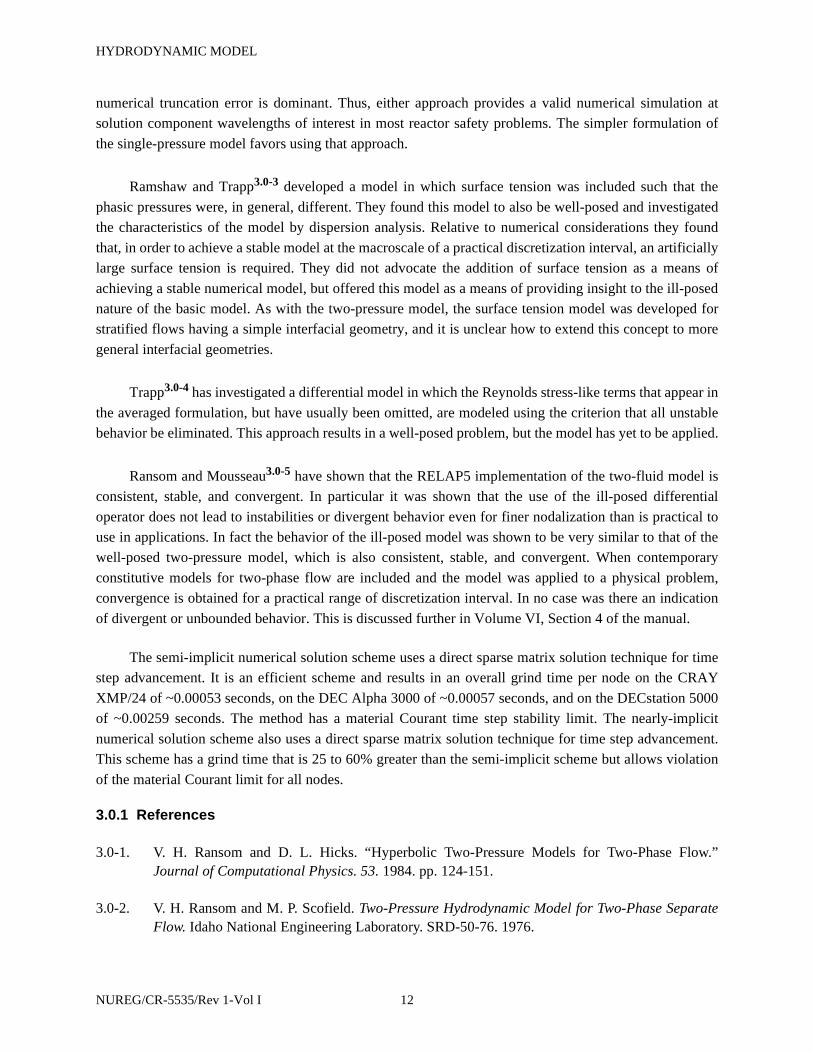
HYDRODYNAMIC MODEL
numerical truncation error is dominant. Thus, either approach provides a valid numerical simulation at
solution component wavelengths of interest in most reactor safety problems. The simpler formulation of
the single-pressure model favors using that approach.
Ramshaw and Trapp3.0-3 developed a model in which surface tension was included such that the
phasic pressures were, in general, different. They found this model to also be well-posed and investigated
the characteristics of the model by dispersion analysis. Relative to numerical considerations they found
that, in order to achieve a stable model at the macroscale of a practical discretization interval, an artificially
large surface tension is required. They did not advocate the addition of surface tension as a means of
achieving a stable numerical model, but offered this model as a means of providing insight to the ill-posed
nature of the basic model. As with the two-pressure model, the surface tension model was developed for
stratified flows having a simple interfacial geometry, and it is unclear how to extend this concept to more
general interfacial geometries.
Trapp3.0-4 has investigated a differential model in which the Reynolds stress-like terms that appear in
the averaged formulation, but have usually been omitted, are modeled using the criterion that all unstable
behavior be eliminated. This approach results in a well-posed problem, but the model has yet to be applied.
Ransom and Mousseau3.0-5 have shown that the RELAP5 implementation of the two-fluid model is
consistent, stable, and convergent. In particular it was shown that the use of the ill-posed differential
operator does not lead to instabilities or divergent behavior even for finer nodalization than is practical to
use in applications. In fact the behavior of the ill-posed model was shown to be very similar to that of the
well-posed two-pressure model, which is also consistent, stable, and convergent. When contemporary
constitutive models for two-phase flow are included and the model was applied to a physical problem,
convergence is obtained for a practical range of discretization interval. In no case was there an indication
of divergent or unbounded behavior. This is discussed further in Volume VI, Section 4 of the manual.
The semi-implicit numerical solution scheme uses a direct sparse matrix solution technique for time
step advancement. It is an efficient scheme and results in an overall grind time per node on the CRAY
XMP/24 of ~0.00053 seconds, on the DEC Alpha 3000 of ~0.00057 seconds, and on the DECstation 5000
of ~0.00259 seconds. The method has a material Courant time step stability limit. The nearly-implicit
numerical solution scheme also uses a direct sparse matrix solution technique for time step advancement.
This scheme has a grind time that is 25 to 60% greater than the semi-implicit scheme but allows violation
of the material Courant limit for all nodes.
3.0.1 References
3.0-1. V. H. Ransom and D. L. Hicks. “Hyperbolic Two-Pressure Models for Two-Phase Flow.”Journal of Computational Physics. 53. 1984. pp. 124-151.
3.0-2. V. H. Ransom and M. P. Scofield. Two-Pressure Hydrodynamic Model for Two-Phase SeparateFlow. Idaho National Engineering Laboratory. SRD-50-76. 1976.
NUREG/CR-5535/Rev 1-Vol I 12
HYDRODYNAMIC MODEL
3.0-3. J. D. Ramshaw and J. A. Trapp. “Characteristics, Stability, and Short-Wavelength Phenomena inTwo-Phase Flow Equation Systems.” Nuclear Science and Engineering. 66. 1978 pp. 93-102.
3.0-4. J. A. Trapp. “The Mean Flow Character of Two-Phase Flow Equations.” International Journal ofMultiphase Flow. 12. 1986. pp. 263-276.
3.0-5. V. H. Ransom and V. A. Mousseau. “Convergence and Accuracy Expectations for Two-PhaseFlow Simulations.” Canadian Nuclear Society International Conference on Simulation Methodsin Nuclear Engineering. Montreal, Canada. 1990.
13 NUREG/CR-5535/Rev 1-Vol I

HYDRODYNAMIC MODEL
NUREG/CR-5535/Rev 1-Vol I 14
Field Equations
3.1 Field Equations
The RELAP5 thermal-hydraulic model solves eight field equations for eight primary dependent
variables. The primary dependent variables are pressure (P), phasic specific internal energies (Ug, Uf),
vapor volume fraction (void fraction) (αg), phasic velocities (vg, vf), noncondensable quality (Xn), and
boron density (ρb). The independent variables are time (t) and distance (x). Noncondensable quality is
defined as the ratio of the noncondensable gas mass to the total gaseous phase mass, i.e., ,
where Mn is the mass of noncondensable in the gaseous phase and Ms is the mass of the steam in the
gaseous phase. The secondary dependent variables used in the equations are phasic densities (ρg, ρf), phasic
temperatures (Tg, Tf), saturation temperature (Ts), and noncondensable mass fraction in noncondensable
gas phase (Xni) for the i-th noncondensable species, i.e.,
(3.1-1)
where Mni is the mass of the i-th noncondensable in the gaseous phase, Mn is the total mass of
noncondensable gas in the gaseous phase, and N is the number of noncondensables.
The basic two-fluid differential equations that form the basis for the hydrodynamic model are next
presented. This discussion will be followed by the development of a convenient form of the differential
equations that is used as the basis for the numerical solution scheme. The modifications necessary to model
horizontal stratified flow are also discussed. Subsequently, the semi-implicit scheme difference equations
and the associated time-advancement scheme are discussed. Next, the nearly-implicit scheme difference
equations and the associated time-advancement scheme are presented. Finally, the volume average
velocity formulations, implicit hydrodynamic/heat structure coupling, and the boron transport equation
numerical solution are presented.
3.1.1 Basic Differential Equations
The differential form of the one-dimensional transient field equations is first presented for a one-
component system. The modifications necessary to consider noncondensables as a component of the
gaseous phase and boron as a nonvolatile solute component of the liquid phase are discussed separately.
3.1.1.1 Vapor/Liquid System.
The basic field equations for the two-fluid nonequilibrium model consist of two phasic continuity
equations, two phasic momentum equations, and two phasic energy equations. The equations are recorded
in differential stream tube form with time and one space dimension as independent variables and in terms
Xn
Mn
Mn Ms+--------------------=
Xni
Mni
Mni
i 1=
N
∑-----------------
Mni
Mn--------= =
15 NUREG/CR-5535/Rev 1-Vol I

Field Equations
of time and volume-average dependent variables.a The development of such equations for the two-phase
process has been recorded in several references3.1-1,3.1-2,3.1-3 and is not repeated here. The equations are
cast in the basic form with discussion of those terms that may differ from other developments.
Manipulations required to obtain the form of the equations from which the numerical scheme was
developed are described in Section 3.1.2.
3.1.1.1.1 Mass Continuity
The phasic continuity equations are
(3.1-2)
(3.1-3)
These equations come from the one-dimensional phasic mass equations [Equation (8.12)] in
Reference 3.1-1 as follows: Equation (8.12) can be written in area average notation wherein the term
has been reduced to . The vapor continuity Equation (3.1-2) then is the same as Equation (8.12) using
k = g. The liquid continuity Equation (3.1-3) then is the same as Equation (8.12) using k = f. This
derivation is discussed in Chapter 8 of Reference 3.1-1.
Generally, the flow does not include mass sources or sinks, and overall continuity consideration
yields the requirement that the liquid generation term be the negative of the vapor generation, that is,
(3.1−4)
The interfacial mass transfer model assumes that total mass transfer can be partitioned into mass
transfer at the vapor/liquid interface in the bulk fluid (Γig) and mass transfer at the vapor/liquid interface in
the boundary layer near the walls (Γw), that is,
(3.1-5)
a. In all the field equations shown herein, the correlation coefficients3.1-1 are assumed to be unity so the average
of a product of variables is equal to the product of the averaged variables.
t∂∂ α gρg( ) 1
A----
x∂∂ αgρgvgA( )+ Γ g=
t∂∂ α fρf( ) 1
A----
x∂∂ α fρfvfA( )+ Γ f=
LV----
1A----
Γ f Γg–=
Γ g Γ ig Γw+=
NUREG/CR-5535/Rev 1-Vol I 16
Field Equations
The Γig term will be developed in the following sections, and the Γw term is determined as part of the
wall heat transfer computation (Section 3.3.10).
3.1.1.1.2 Momentum Conservation
The phasic conservation of momentum equations are used, and recorded here, in an expanded form
and in terms of momenta per unit volume using the phasic primitive velocity variables vg and vf. The
spatial variation of momentum term is expressed in terms of and . This form has the desirable feature
that the momentum equation reduces to Bernoulli’s equations for steady, incompressible, and frictionless
flow. A guiding principle used in the development of the RELAP5 momentum formulation is that
momentum effects are secondary to mass and energy conservation in reactor safety analysis and a less
exact formulation (compared to mass and energy conservation) is acceptable, especially since nuclear
reactor flows are dominated by large sources and sinks of momentum (i.e., pumps, abrupt area change). A
primary reason for use of the expanded form is that is it more convenient for development of the numerical
scheme. The momentum equation for the vapor phase is
(3.1-6)
and for the liquid phase is
(3.1-7)
These equations come from the one-dimensional phasic momentum equations [Equation (8.13)] in
Reference 3.1-1 with the following simplifications: the Reynolds stresses are neglected, the phasic
pressures are assumed equal, the interfacial pressure is assumed equal to the phasic pressures (except for
stratified flow), the covariance terms are universally neglected (unity assumed for covariance multipliers),
interfacial momentum storage is neglected, phasic viscous stresses are neglected, the interface force terms
consist of both pressure and viscous stresses, and the normal wall forces are assumed adequately modeled
by the variable area momentum flux formulation. The phasic continuity equations are multiplied by the
corresponding phasic velocity, and are subtracted from the momentum equations. The vapor momentum
Equation (3.1-6) is the same as the resulting vapor momentum equation from Equation (8.13) using k = g;
vg2 vf
2
α gρgA∂vg
∂t--------
12---αgρgA
∂vg2
∂x--------+ αgA
∂P∂x------– αgρgBxA α gρgA( )FWG vg( )–+=
Γ gA vgI vg–( ) α gρgA( )FIG vg vf–( )–+
Cα gα fρmA∂ vg vf–( )
∂t----------------------- vf
∂vg
∂x-------- vg
∂vf
∂x-------–+–
α fρfA∂vf
∂t-------
12---α fρfA
∂vf2
∂x--------+ α fA
∂P∂x------– α fρfBxA α fρfA( )FWF vf( )–+=
– ΓgA vfI vf–( ) α fρfA( )FIF vf vg–( )–
Cα fαgρmA∂ vf vg–( )
∂t----------------------- vg
∂vf
∂x------- vf
∂vg
∂x--------–+–
17 NUREG/CR-5535/Rev 1-Vol I

Field Equations
the liquid momentum Equation (3.1-7) is the same as the resulting liquid momentum equation from
Equation (8.13) using k = f. This is discussed in Chapter 8 of Reference 3.1-1.
The force terms on the right sides of Equation (3.1-6) and Equation (3.1-7) are, respectively, the
pressure gradient, the body force (i.e., gravity and pump head), wall friction, momentum transfer due to
interface mass transfer, interface frictional drag, and force due to virtual mass. The terms FWG and FWF
are part of the wall frictional drag, which are linear in velocity, and are products of the friction coefficient,
the frictional reference area per unit volume, and the magnitude of the fluid bulk velocity. The interfacial
velocity in the interface momentum transfer term is the unit momentum with which phase appearance or
disappearance occurs. The coefficients FIG and FIF are part of the interface frictional drag; two different
models (drift flux and drag coefficient) are used for the interface friction drag, depending on the flow
regime. The coefficient of virtual mass is based on that used by Anderson3.1-4 in the RISQUE code, where
the value for C depends on the flow regime. A value of C > 1/2 has been shown to be appropriate for
bubbly or dispersed flows,3.1-5, 3.1-6 while C = 0 may be appropriate for a separated or stratified flow. At
present, a value of C > 1/2 is used for all flow regimes. This is discussed in Section 3.3.
The virtual mass term listed in Equation (3.1-6) and Equation (3.1-7) is the same objective
formulation3.1-7, 3.1-8 used in RELAP5/MOD1. In the RELAP5/MOD3 coding, however, this term is
simplified. In particular, the spatial derivative portion of the term is neglected. The reason for this change
is that inaccuracies in approximating the spatial derivative portion of the term for the relatively coarse
nodalizations used in system representations can lead to nonphysical characteristics in the numerical
solution. The primary effect of the virtual mass term is on the mixture sound speed; thus, the simplified
form is adequate, since critical flows are calculated in RELAP5 using an integral model3.1-9 in which the
sound speed is based on an objective formulation for the added mass terms.
Conservation of momentum at the interface requires that the force terms associated with interface
mass and momentum exchange sum to zero, and is shown as
(3.1-8)
where the spatial derivatives have been eliminated as explained above.
This particular form for interface momentum balance results from consideration of the momentum
equations in unexpanded form. The force terms associated with virtual mass acceleration in Equation (3.1-
8) sum to zero identically as a result of the particular form chosen. In addition, it is usually assumed
(although not required by any basic conservation principle) that the interface momentum transfer due to
friction and due to mass transfer independently sum to zero, that is,
ΓgAvgI αgρgA( )FIG vg vf–( )– Cαgα fρmA∂ vg vf–( )
∂t-----------------------–
ΓgAvfI– α fρfA( )FIF vf vg–( )– Cα fαgρmA∂ vf vg–( )
∂t-----------------------– 0=
NUREG/CR-5535/Rev 1-Vol I 18

Field Equations
(3.1-9)
and
(3.1−10)
These conditions are sufficient to ensure that Equation (3.1-8) is satisfied.
3.1.1.1.3 Energy Conservation
The phasic thermal energy equations are
(3.1-11)
(3.1-12)
These equations come from the one-dimensional phasic thermal energy equations [Equation (8.16)]
in Reference 3.1-1 with the following simplifications: the Reynolds heat flux is neglected, the covariance
terms are universally neglected (unity assumed for covariance multipliers), interfacial energy storage is
neglected, and internal phasic heat transfer is neglected. The vapor thermal energy Equation (3.1-11) is the
same as the resulting vapor thermal energy equation from Equation (8.16) using k = g; the liquid thermal
energy Equation (3.1-12) is the same as the resulting liquid thermal energy equation from Equation (8.16)
using k = f. This derivation is discussed in Chapter 8 of Reference 3.1-1.
In the phasic energy equations, Qwg and Qwf are the phasic wall heat transfer rates per unit volume
(see Section 3.3.9). These phasic wall heat transfer rates satisfy the equation
(3.1-13)
where Q is the total wall heat transfer rate to the fluid per unit volume.
The phasic enthalpies associated with bulk interface mass transfer in Equation (3.1-11)
and Equation (3.1-12) are defined in such a way that the interface energy jump conditions at the liquid-
vapor interface are satisfied. In particular, the and are chosen to be and hf, respectively, for the
vgI vfI vI= =
α gρgFIG α fρfFIF αgα fρgρfFI= =
t∂∂ α gρgUg( ) 1
A----
x∂∂ αgρgUgvgA( )+ P
∂αg
∂t---------
PA----
x∂∂ αgvgA( )––=
Q+ wg Qig Γ ighg* Γwhg
′ DISSg+ + + +
t∂∂ α fρfUf( ) 1
A----
x∂∂ α fρfUfvfA( )+ P
∂α f
∂t--------
PA----
x∂∂ α fvfA( )––=
Q+ wf Qif Γ ig– hf* Γw– hf
′ DISSf+ +
Q Qwg Qwf+=
hg* hf
* ,( )
hg* hf
* hgs
19 NUREG/CR-5535/Rev 1-Vol I

Field Equations
case of vaporization and hg and , respectively, for the case of condensation. The same is true for the
phasic enthalpies associated with wall (thermal boundary layer) interface mass transfer. The logic
for this choice will be further explained in the development of the mass transfer (vapor generation) model.
Vapor Generation
The vapor generation (or condensation) consists of two parts, vapor generation which results from
energy exchange (Γig) and vapor generation due to wall heat transfer effects (Γw) [see Equation (3.1-5)].
Each of the vapor generation (or condensation) processes involves interface heat transfer effects. The
interface heat transfer terms (Qig and Qif) appearing in Equation (3.1-11) and Equation (3.1-12) include
heat transfer from the fluid states to the interface due to interface energy exchange in the bulk and in the
thermal boundary layer near the wall. The vapor generation (or condensation) rates are established from
energy balance considerations at the interface.
The summation of Equation (3.1-11) and Equation (3.1-12) produces the mixture energy equation,
from which it is required that the interface transfer terms sum to zero, that is,
(3.1-14)
The interface heat transfer terms (Qig and Qif) consist of two parts, that is, interface heat transfer in
the bulk and interface heat transfer in the thermal boundary layer near the wall
. This is one situation where the assumption of no transverse gradients needs to be
supplemented by a special model. The interface heat transfer terms are shown in Figure 3.1-1 for the case
of subcooled boiling.
The two parts are additive, that is,
(3.1-15)
and
(3.1-16)
The bulk interface heat transfer is at the steam-liquid interface in the bulk. This represents thermal
energy exchange between the fluid interface (at the saturation temperature Ts corresponding to the total
pressure P) and the bulk fluid state.
hfs
hg′ hf
′,( )
Qig Qif Γ ig hg* hf
*–( ) Γw hg′ hf
′–( )+ + + 0=
QigB and Qif
B( )
QigW and Qif
W( )
Qig QigB Qig
W+=
Qif QifB Qif
W+=
NUREG/CR-5535/Rev 1-Vol I 20
Field Equations
For gas, the bulk interface heat transfer is given by
(3.1-17)
where Hig is the gas interface heat transfer coefficient per unit volume and Tg is the gas temperature.
For liquid, the bulk interface heat transfer is given by
(3.1-18)
where Hif is the liquid interface heat transfer coefficient per unit volume and Tf is the liquid temperature.
The terms are the interface heat transfer rates near the wall and will be defined in terms
of the wall vapor generation (or condensation) process. This is discussed in more detail in Volume IV.
Inserting Equation (3.1-17) and Equation (3.1-18) into Equation (3.1-15) and Equation (3.1-16) gives
(3.1-19)
and
(3.1-20)
Figure 3.1-1 Interface heat transfer in the bulk and near the wall for subcooled boiling
Qif Qif
Qig
w B
B
WALL
QigB Hig Ts Tg–( )=
QifB Hif Ts Tf–( )=
QigW and Qif
W
Qig Hig Ts Tg–( ) QigW+=
Qif Hif Ts Tf–( ) QifW+=
21 NUREG/CR-5535/Rev 1-Vol I
Field Equations
Although it is not a fundamental requirement, it is assumed that Equation (3.1-14) will be satisfied by
requiring that the bulk interface energy exchange terms and the near wall interface energy exchange terms
each sum to zero independently. Thus,
(3.1-21)
and
(3.1-22)
In addition, since it is assumed that vapor appears at saturation, it follows that for boiling
processes in the boundary layer near the wall. Equation (3.1-22) can then be used to solve for the interface
vaporization rate in the boundary layer near the walls
(3.1-23)
Similarly, since it is assumed that liquid appears at saturation, it follows that for
condensation processes in the boundary layer near the wall. Equation (3.1-22) can then be used to solve for
the interface condensation rate in the boundary layer near the walls
(3.1-24)
Solving Equation (3.1-23) and Equation (3.1-24) for and , and substituting these terms into
Equation (3.1-19) and Equation (3.1-20), the interface energy transfer terms, Qig and Qif, can thus be
expressed in a general way as
(3.1-25)
and
(3.1-26)
Hig Ts Tg–( ) Hif Ts Tf–( ) Γ ig hg* hf
*–( )+ + 0=
QigW Qif
W Γw hg′ hf
′–( )+ + 0=
QigW 0=
Γw
QifW–
hg′ hf
′–---------------=
QifW 0=
Γw
QigW–
hg′ hf
′–---------------=
QifW Qig
W
Qig Hig Ts Tg–( ) 1 ε–2
----------- Γw hg
′ hf′–( )–=
Qif Hif Ts Tf–( ) 1 ε+2
------------ Γw hg
′ hf′–( )–=
NUREG/CR-5535/Rev 1-Vol I 22

Field Equations
where ε = 1 for boiling in the boundary layer near the wall, and ε = -1 for condensation in the boundary
layer near the wall. Finally, Equation (3.1-14) can be used to solve for the interface vaporization (or
condensation) rate in the bulk fluid
(3.1-27)
which, upon substitution of Equation (3.1-25) and Equation (3.1-26), becomes
(3.1-28)
The phase change process that occurs at the interface is envisioned as a process in which bulk fluid is
heated or cooled to the saturation temperature and phase change occurs at the saturation state. The
interface energy exchange process from each phase must be such that at least the sensible energy change to
reach the saturation state occurs. Otherwise, it can be shown that the phase change process implies energy
transfer from a lower temperature to a higher temperature. Such conditions can be avoided by the proper
choice of the variables and for bulk interface mass transfer as well as and for near wall
interface mass transfer. In particular, it can be shown that and should be
(3.1-29)
and
(3.1-30)
where
η = 1 for Γig > 0
= -1 for Γig < 0
For flashing or isothermal cases, , and . For condensing cases, ,
and .
Γ ig
Qig Qif+
hg* hf
* –---------------------– Γw
hg′ hf
′–( )hg
* hf* –
--------------------–=
Γ ig Hig Ts Tg–( ) Hif Ts Tf–( )+
hg* hf
* –-----------------------------------------------------------------–=
hg* hf
* hg′ hf
′
hg* hf
*
hg* 1
2--- hg
s hg+( ) η hgs hg–( )+[ ]=
hf* 1
2--- hf
s h+ f( ) η– hfs hf–( )[ ]=
η 1= hf* hf= hg
* hgs= η 1–= hf
* hfs=
hg* hg=
23 NUREG/CR-5535/Rev 1-Vol I
Field Equations
It can also be shown that and should be
(3.1-31)
and
(3.1-32)
where
ε = 1 for Γw > 0
= -1 for Γw < 0
For flashing or isothermal cases, , and . For condensing cases, ,
and .
Substituting Equation (3.1-28) into Equation (3.1-5) gives the final expression for the total interface
mass transfer as
(3.1-33)
Volume IV of the manual discusses the energy partitioning in more detail.
3.1.1.1.4 Dissipation Terms
The phasic energy dissipation terms, DISSg and DISSf, are the sums of wall friction and pump
effects. The dissipation effects due to interface mass transfer, interface friction, and virtual mass are
neglected. This is a reasonable assumption since these terms are small in magnitude in the energy equation.
In the mass and momentum equations, interface mass transfer, interface friction, and virtual mass are
important and are not neglected. The wall friction dissipations are defined as
(3.1-34)
and
hg′ hf
′
hg′ 1
2--- hg
s hg+( ) ε hgs hg–( )+[ ]=
hf′ 1
2--- hf
s hf+( ) ε– hfs hf–( )[ ]=
Γw 0≥ hf′ hf= hg
′ hgs= Γw 0< hf
′ hfs=
hg′ hg=
Γg
Hig Ts Tg–( ) Hif Ts Tf–( )+
hg* hf
* –-----------------------------------------------------------------– Γw+=
DISSg αgρg FWG vg2=
NUREG/CR-5535/Rev 1-Vol I 24
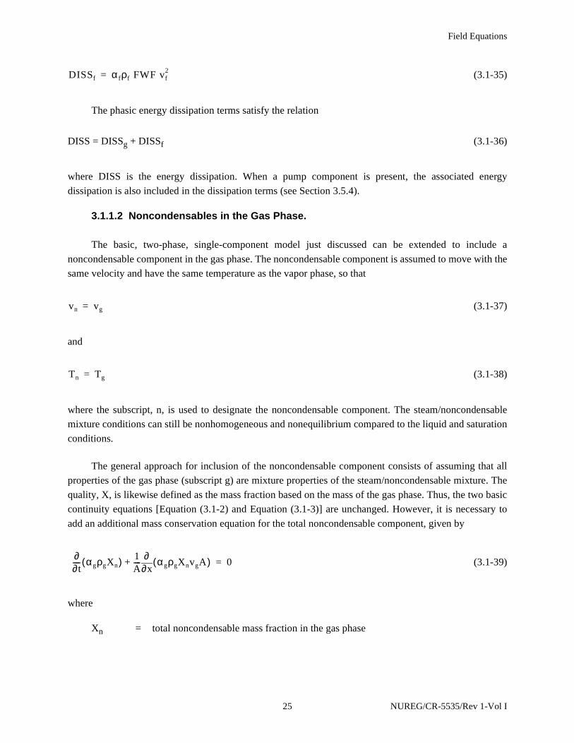
Field Equations
(3.1-35)
The phasic energy dissipation terms satisfy the relation
DISS = DISSg + DISSf (3.1-36)
where DISS is the energy dissipation. When a pump component is present, the associated energy
dissipation is also included in the dissipation terms (see Section 3.5.4).
3.1.1.2 Noncondensables in the Gas Phase.
The basic, two-phase, single-component model just discussed can be extended to include a
noncondensable component in the gas phase. The noncondensable component is assumed to move with the
same velocity and have the same temperature as the vapor phase, so that
(3.1-37)
and
(3.1-38)
where the subscript, n, is used to designate the noncondensable component. The steam/noncondensable
mixture conditions can still be nonhomogeneous and nonequilibrium compared to the liquid and saturation
conditions.
The general approach for inclusion of the noncondensable component consists of assuming that all
properties of the gas phase (subscript g) are mixture properties of the steam/noncondensable mixture. The
quality, X, is likewise defined as the mass fraction based on the mass of the gas phase. Thus, the two basic
continuity equations [Equation (3.1-2) and Equation (3.1-3)] are unchanged. However, it is necessary to
add an additional mass conservation equation for the total noncondensable component, given by
(3.1-39)
where
Xn = total noncondensable mass fraction in the gas phase
DISSf α fρf FWF vf2=
vn vg=
Tn Tg=
∂∂t---- αgρgXn( ) 1
A----
x∂∂ αgρgXnvgA( )+ 0=
25 NUREG/CR-5535/Rev 1-Vol I

Field Equations
= (3.1-40)
Mni = mass of i-th noncondensable gas
Mn = total mass of noncondensable gas in the gaseous phase
Ms = mass of steam in the gas phase
N = number of noncondensables.
For each noncondensable specie, the mass conservation equation is
(3.1-41)
where Xni is defined in Equation (3.1-1). Only N-1 of the noncondensable gas specie equations need to be
solved since the mass fraction of the N-th specie can be found as the difference between the total
noncondensable gas mass fraction and the sum of the N-1 noncondensable gas specie mass fractions.
The energy equations are modified to include the sensible interface (direct) heating term Qgf. This
term is necessary because the interfacial terms use saturation temperature based on the bulk steam partial
pressure rather than saturation temperature based on the local (interface) steam partial pressure. This is
another situation in which the assumption of no transverse gradients in the one-dimensional formulation of
the conservation equations needs to be supplemented by a special model. The energy field equations have
the form
(3.1-42)
(3.1-43)
The term Qgf in Equation (3.1-42) and Equation (3.1-43) is the sensible heat transfer rate per unit
volume. This is the heat transfer at the noncondensable gas-liquid interface, and it represents thermal
Mni
i 1=
N
∑
Mni Ms+
i 1=
N
∑---------------------------------
Mn
Mn Ms+---------------------=
∂∂t---- αgρgXnXni( ) 1
A----
x∂∂ αgρgXnXnivgA( )+ 0=
∂∂t---- α gρgUg( ) 1
A----
∂∂x------ αgρgUgvgA( )+ P
∂αg
∂t---------–
PA----
∂∂x------ α gvgA( )–=
Qwg Qig Γ ighg* Γwhg
′ Qgf– DISSg+ + + + +
∂∂t---- α fρfUf( ) 1
A----
∂∂x------ α fρfUfvfA( )+ P
∂α f
∂t--------–
PA----
∂∂x------ α fvfA( )–=
Qwf Qif Γ ig– hf* Γw– hf
′ Q+ gf DISSf+ + +
NUREG/CR-5535/Rev 1-Vol I 26

Field Equations
energy exchange between the bulk fluid states themselves when noncondensable gas is present. This term
is given by
(3.1-44)
where Hgf is the sensible (direct) heat transfer coefficient per unit volume. This makes use of Dalton’s law
(P = Ps + Pn), where Pn is the noncondensable gas partial pressure. This term is similar to the heat
conduction term in the accumulator model (see Section 3.5.7.2). The multiplier based on the difference in
the total pressure and the partial pressure of steam is an ad-hoc function used to turn off this term when
there is no noncondensable gas in the volume. The value of the heat transfer coefficient depends upon the
configuration of the interface (i.e., flow regime) between the liquid and the noncondensable gas just like
the situation for the steam-liquid interface.
The interfacial heat transfer and mass transfer terms are also modified when noncondensables are
present. The gas bulk interface heat transfer [Equation (3.1-17)] now has the form
(3.1-45)
where the fluid interface is assumed to be at the saturation temperature Ts(Ps) corresponding to the partial
pressure of steam (Ps).
Thus, the total gas interfacial heat transfer [Equation (3.1-19)] now has the form
(3.1-46)
The assumption that the bulk interface exchange terms sum to zero [Equation (3.1-21)], now has the
form
(3.1-47)
Thus, the total gas interface energy transfer term [Equation (3.1-25)] is now expressed as
(3.1-48)
Qgf
P Ps–P
-------------- Hgf Tg Tf–( )
Pn
P-----Hgf Tg Tf–( )= =
QigB Ps
P-----Hig Ts Ps( ) Tg–[ ]=
Qig
Ps
P-----Hig Ts Ps( ) Tg–[ ] Qig
W+=
Ps
P-----Hig Ts Ps( ) Tg–[ ] Hif Ts Ps( ) Tf–[ ] Γ ig hg
* hf*–( )+ + 0=
Qig
Ps
P-----Hig Ts Ps( ) Tg–[ ] 1 ε–
2-----------
Γw hg′ hf
′–( )–=
27 NUREG/CR-5535/Rev 1-Vol I
Field Equations
The bulk interface mass transfer rate [Equation (3.1-28)] now has the form
(3.1-49)
and the total interface mass transfer rate [Equation (3.1-33)] now has the form
(3.1-50)
Volume IV of the manual discusses the energy partitioning in more detail.
The gas enthalpy , which is used in the energy field equations and in the mass transfer Γg, is based
on the partial pressure of steam instead of the total pressure when noncondensables are present.
The momentum field equations are unchanged when noncondensables are present. In all the
equations, the vapor field properties are now evaluated for the steam/noncondensable mixture. The
modifications appropriate to the state relationships are discussed in Section 3.2.3.
3.1.1.3 Boron Concentration in the Liquid Field.
An Eulerian boron tracking model is used in RELAP5 that simulates the transport of a dissolved
component in the liquid phase. The solution is assumed to be sufficiently dilute that the following
assumptions are valid:
• Liquid properties are not altered by the presence of the solute.
• Solute is transported only in the liquid phase and at the velocity of the liquid phase.
• Energy transported by the solute is negligible.
• Inertia of the solute is negligible.
Under these assumptions, only an additional field equation for the conservation of the solute is
required. In differential form, the added equation is
(3.1-51)
Γ ig
Ps
P-----Hig Ts Ps( ) Tg–[ ] Hif Ts Ps( ) Tf–[ ]+
hg* hf
*–-------------------------------------------------------------------------------------------–=
Γ g
Ps
P-----Hig Ts Ps( ) Tg–[ ] Hif Ts Ps( ) Tf–[ ]+
hg* hf
*–-------------------------------------------------------------------------------------------– Γw+=
hg*
∂ρb
∂t--------
1A----
∂ ρbvfA( )∂x
-----------------------+ 0=
NUREG/CR-5535/Rev 1-Vol I 28
Field Equations
where the spatial boron density, ρb, is defined as
(3.1-52)
Cb is the concentration of boron (mass of boron per mass of liquid), ρb is the spatial boron density
(mass of boron per total volume of liquid and gas), and X is the static quality.
3.1.1.4 Stratified Flow.
Flow at low velocity in a horizontal pipe can be stratified as a result of buoyancy forces caused by
density differences between vapor and liquid. When the flow is stratified, the area average pressures are
affected by nonuniform transverse distribution of the phases. Appropriate modifications to the basic field
equations when stratified flow exists are obtained by considering separate area average pressures for the
vapor and liquid phases and the interfacial pressure between them. Using this model, the pressure gradient
force terms of Equation (3.1-6) and Equation (3.1-7) become
(3.1-53)
and
(3.1-54)
The area average pressure for the entire cross-section of the flow is expressed in terms of the phasic
area average pressures by
(3.1-55)
With these definitions, the sum of the phasic momentum equations, written in terms of the cross-
section average pressure (see Section 3.1.2) remains unchanged. However, the difference of the phasic
momentum equations (see Section 3.1.2), contains the following additional terms on the right side
(3.1-56)
ρb α fρfCb ρm 1 X–( )Cb= =
αgA∂P∂x------ →– αgA
∂Pg
∂x--------– PI Pg– A
∂αg
∂x---------+
α fA∂P∂x------ →– α fA
∂Pf
∂x--------– PI Pf– A
∂α f
∂x--------+
P α gPg α fPf+=
ραgα fρgρf----------------------
α f
∂ α gPg( )∂x
-------------------– αg
∂ α fPf( )∂x
------------------ PI
∂αg
∂x---------+ +
29 NUREG/CR-5535/Rev 1-Vol I
Field Equations
The interface and phasic cross-sectional average pressures, PI, Pg, and Pf, can be found by means of
the assumption of a transverse hydrostatic pressure in a round pipe. For a pipe having diameter D,
pressures PI, Pg, and Pf are given by
(3.1-57)
(3.1-58)
where By equals the transverse body force (ordinarily equal to -g).
The central angle, θ, is defined by the void fraction, as illustrated in Figure 3.1-2. The algebraic
relationship between αg and θ is
(3.1−59)
The additional terms in the difference of the momentum equations [Equation (3.1-56)] can be
simplified using Equation (3.1-57), (3.1-58), and (3.1-59) to obtain the term
(3.1-60)
Figure 3.1-2 Relation of central angle to void fraction
Pg PI ρgByDsin3θ3παg------------
θcos2
------------– –=
Pf PI ρfByDsin3θ3παf------------
θcos2
------------– –=
Liquid
Vaporθ
°
Vapor area = αgA
Liquid area = αfA
θ αg
α gπ θ θ θcossin–=
ρm
ρgρf----------
– ρf ρg–( )πDBy
4 θsin--------------
∂αg
∂x---------
NUREG/CR-5535/Rev 1-Vol I 30
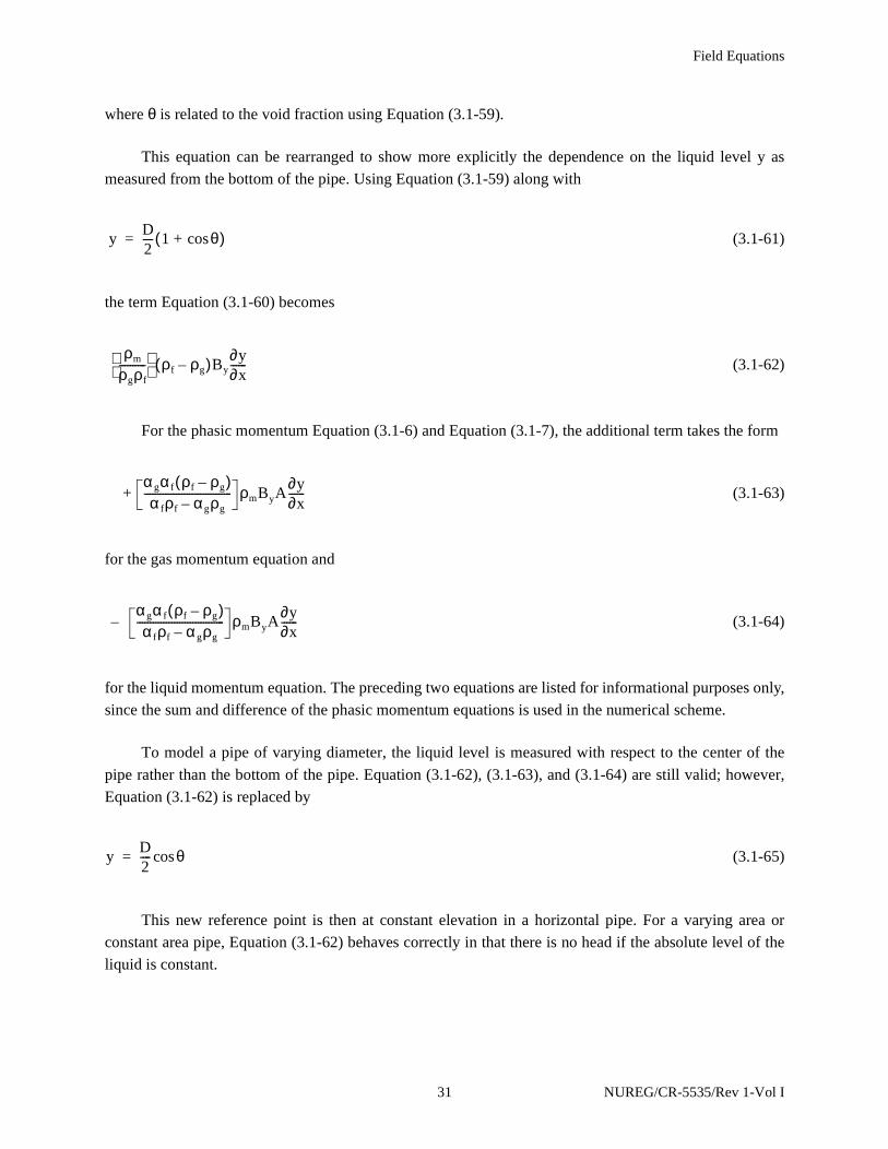
Field Equations
where θ is related to the void fraction using Equation (3.1-59).
This equation can be rearranged to show more explicitly the dependence on the liquid level y as
measured from the bottom of the pipe. Using Equation (3.1-59) along with
(3.1-61)
the term Equation (3.1-60) becomes
(3.1-62)
For the phasic momentum Equation (3.1-6) and Equation (3.1-7), the additional term takes the form
(3.1-63)
for the gas momentum equation and
(3.1-64)
for the liquid momentum equation. The preceding two equations are listed for informational purposes only,
since the sum and difference of the phasic momentum equations is used in the numerical scheme.
To model a pipe of varying diameter, the liquid level is measured with respect to the center of the
pipe rather than the bottom of the pipe. Equation (3.1-62), (3.1-63), and (3.1-64) are still valid; however,
Equation (3.1-62) is replaced by
(3.1-65)
This new reference point is then at constant elevation in a horizontal pipe. For a varying area or
constant area pipe, Equation (3.1-62) behaves correctly in that there is no head if the absolute level of the
liquid is constant.
yD2---- 1 θcos+( )=
ρm
ρgρf----------
ρf ρg–( )By∂y∂x------
α gα f ρf ρg–( )α fρf αgρg–
--------------------------------- ρmByA∂y∂x------+
–αgα f ρf ρg–( )α fρf α gρg–
--------------------------------- ρmByA∂y∂x------
yD2---- θcos=
31 NUREG/CR-5535/Rev 1-Vol I
Field Equations
To take account of possible orifices, a junction diameter is estimated and the horizontal volume
liquid levels are restrained to be within the range of this diameter. Thus, in the limit of a closed junction
there will be no driving head term.
A RELAP5 horizontal pipe need not be absolutely horizontal; it can have a slope of angle Φ. There
may also be a change of slope at the junction between two volumes. The modeling for this does not have a
firm physical basis but has appropriate limiting behavior. The volume liquid levels are multiplied by cosΦwhich is unity for a horizontal volume. If the slopes of the two volumes are different then an extra term is
added to the level difference. This term is proportional to the sine of the difference of the absolute values
of the two slope angles. The sign and magnitude of the “constant” of proportionality are such that the
following two conditions are met:
1. When a vertical volume is above a horizontal volume, the liquid level difference termis zero.
2. When a vertical volume is below a horizontal volume, the liquid level difference termis as if the liquid level in the vertical volume is at the bottom of the connecting orifice.
The above two limits ensure that liquid is not pushed upward, but can drain if required. When non-
horizontal volumes have a significant liquid content, the normal head terms will be dominant.
The additional force term that arises for a stratified flow geometry in horizontal pipes is added to the
basic equation when the flow is established to be stratified from flow regime considerations. Note that the
additional force term was derived assuming a round pipe. If the cross-section is rectangular, this
assumption is not valid.
A similar term is added when there is stratified flow in a series of cells defined as vertically oriented
but are cross-connected in the horizontal direction. Equation (3.1-62), (3.1-63), and (3.1-64) are still used;
however, Equation (3.1-61) is replaced with
(3.1-66)
where ∆z is the height of the volume.
In order to provide for a smooth transition between stratified and nonstratified flow situations, this
term is activated in all flow regimes. Since this term is small compared to other terms in the momentum
equation when the flow is nonstratified, this is a reasonable assumption.
y1 2αg–
2------------------∆z=
NUREG/CR-5535/Rev 1-Vol I 32

Field Equations
3.1.2 Numerically Convenient Set of Differential Equations
A more convenient set of differential equations upon which to base the numerical scheme is obtained
from the basic density and energy differential equations by expanding the time derivative in each equation
using the product rule. When the product rule is used to evaluate the time derivative, we will refer to this
form as the expanded form. The mass and momentum equations are used as sum and difference equations
in the numerical scheme and are recorded here in that form. The reason for using this form is ease of
degeneration of the model to the single-phase case.
A sum density equation is obtained by expanding the time derivative in the phasic density equations,
Equation (3.1-2) and (3.1-3), adding these two new equations, and using the relation
(3.1-67)
This gives
(3.1-68)
A difference density equation is obtained by expanding the time derivative in the phasic density
equations, Equation (3.1-2) and (3.1-3), subtracting these two new equations, again using the relation
(3.1-69)
and substituting Equation (3.1-50) for Γg. This gives
(3.1-70)
The time derivative of the total noncondensable density equation, Equation (3.1-39), is expanded to
give
(3.1−71)
∂α f
∂t--------
∂αg
∂t---------–=
αg
∂ρg
∂t-------- α f
∂ρf
∂t-------- ρg ρf–( )
∂αg
∂t---------
1A----
x∂∂ αgρgvgA α fρfvfA+( )+ + + 0=
∂α f
∂t--------
∂αg
∂t---------–=
α g
∂ρg
∂t-------- α f
∂ρf
∂t--------– ρg ρf+( )
∂αg
∂t---------
1A----
x∂∂ αgρgvgA α fρfvfA–( )+ +
2Ps
P-----Hig Ts Tg–( ) Hif Ts Tf–( )+
hg* hf
*–--------------------------------------------------------------------------------– 2Γw+=
ρgXn
∂α g
∂t--------- αgXn
∂ρg
∂t-------- αgρg
∂Xn
∂t---------
1A----
∂∂x------ αgρgXnvgA( )+ + + 0=
33 NUREG/CR-5535/Rev 1-Vol I

Field Equations
The time derivative of the individual noncondensable density equation, Equation (3.1-41), is not
expanded, since the individual noncondensable quality, Xni, will be obtained from the unexpanded
equation (Section 3.1.4.1).
The momentum equations are also rearranged into a sum and difference form. The sum momentum
equation is obtained by direct summation of Equation (3.1-6) and (3.1-7) with the interface conditions
[Equation (3.1-8) through (3.1-10)] substituted where appropriate and the cross-sectional area canceled
throughout. The resulting sum equation is
(3.1−72)
The difference of the phasic momentum equations is obtained by first dividing the vapor and liquid
phasic momentum equations [Equation (3.1-6) and Equation (3.1-7)] by αgρgA and αfρfA, respectively,
and subtracting. Here again, the interface conditions are used, and the common area is divided out. As
previously discussed, the virtual mass term is simplified by neglecting the spatial derivative portion and
the additional stratified force term (see Section 3.1.1.4) is added. The resulting equation is
(3.1-73)
where the interfacial velocity, vI, is defined as
(3.1-74)
This definition for vI has the property that if λ = 1/2 the interface momentum transfer process
associated with mass transfer is reversible. This value leads to either an entropy sink or source, depending
on the sign of Γg. However, if λ is chosen to be 0 for positive values of Γg and +1 for negative values of Γg
(that is, a donor formulation), the mass exchange process is always dissipative. The latter model for vI is
the most realistic for the momentum exchange process and is used for the numerical scheme development.
α gρg
∂vg
∂t-------- α fρf
∂vf
∂t-------
12---αgρg
∂vg2
∂x--------
12---α fρf
∂vf2
∂x--------+ + +
∂P∂x------– ρmBx+=
αgρgFWGvg– α fρfFWFvf– Γ g vg vf–( )–
∂vg
∂t--------
∂vf
∂t-------–
12---
∂vg2
∂x--------
12---
∂vf2
∂x--------–+
1ρg-----
1ρf----–
∂P∂x------–=
FWGvg F+ WFvf–
Γ g ρmvI α fρfvg α gρgvf+( )–[ ]αgρgα fρf
------------------------------------------------------------------------ ρmFI vg vf–( )–+
Cρm
2
ρgρf----------
∂ vg vf–( )∂t
-----------------------–ρm
ρgρf----------
ρf ρg–( )By∂y∂x------+
vI λvg 1 λ–( )vf+=
NUREG/CR-5535/Rev 1-Vol I 34
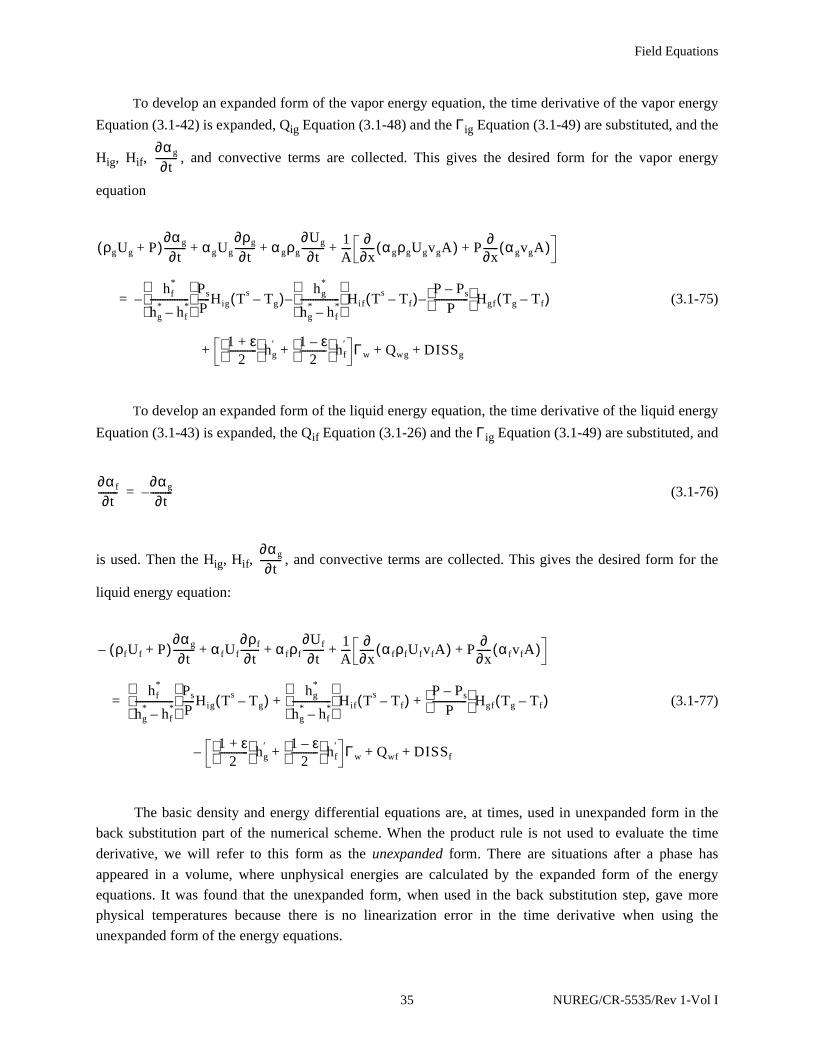
Field Equations
To develop an expanded form of the vapor energy equation, the time derivative of the vapor energy
Equation (3.1-42) is expanded, Qig Equation (3.1-48) and the Γig Equation (3.1-49) are substituted, and the
Hig, Hif, , and convective terms are collected. This gives the desired form for the vapor energy
equation
(3.1-75)
To develop an expanded form of the liquid energy equation, the time derivative of the liquid energy
Equation (3.1-43) is expanded, the Qif Equation (3.1-26) and the Γig Equation (3.1-49) are substituted, and
(3.1-76)
is used. Then the Hig, Hif, , and convective terms are collected. This gives the desired form for the
liquid energy equation:
(3.1-77)
The basic density and energy differential equations are, at times, used in unexpanded form in the
back substitution part of the numerical scheme. When the product rule is not used to evaluate the time
derivative, we will refer to this form as the unexpanded form. There are situations after a phase has
appeared in a volume, where unphysical energies are calculated by the expanded form of the energy
equations. It was found that the unexpanded form, when used in the back substitution step, gave more
physical temperatures because there is no linearization error in the time derivative when using the
unexpanded form of the energy equations.
∂αg
∂t---------
ρgUg P+( )∂α g
∂t--------- αgUg
∂ρg
∂t-------- α gρg
∂Ug
∂t---------
1A----
∂∂x------ αgρgUgvgA( ) P
∂∂x------ α gvgA( )++ + +
hf*
hg* hf
*–----------------
Ps
P-----Hig Ts Tg–( )–
hg*
hg* hf
*–----------------
Hif Ts Tf–( )–P P– s
P--------------
– Hgf Tg Tf–( )=
1 ε+2
------------ hg
′ 1 ε–2
----------- hf
′+ Γw Qwg DISSg+ + +
∂α f
∂t--------
∂αg
∂t---------–=
∂αg
∂t---------
ρfUf P+( )∂α g
∂t---------– α fUf
∂ρf
∂t-------- α fρf
∂Uf
∂t---------
1A----
∂∂x------ α fρfUfvfA( ) P
∂∂x------ α fvfA( )++ + +
hf*
hg* hf
*–----------------
Ps
P-----Hig Ts Tg–( )
hg*
hg* hf
*–----------------
Hif Ts Tf–( )P P– s
P--------------
Hgf Tg Tf–( )+ +=
1 ε+2
------------ hg
′ 1 ε–2
----------- hf
′+ Γw– Qwf DISSf+ +
35 NUREG/CR-5535/Rev 1-Vol I
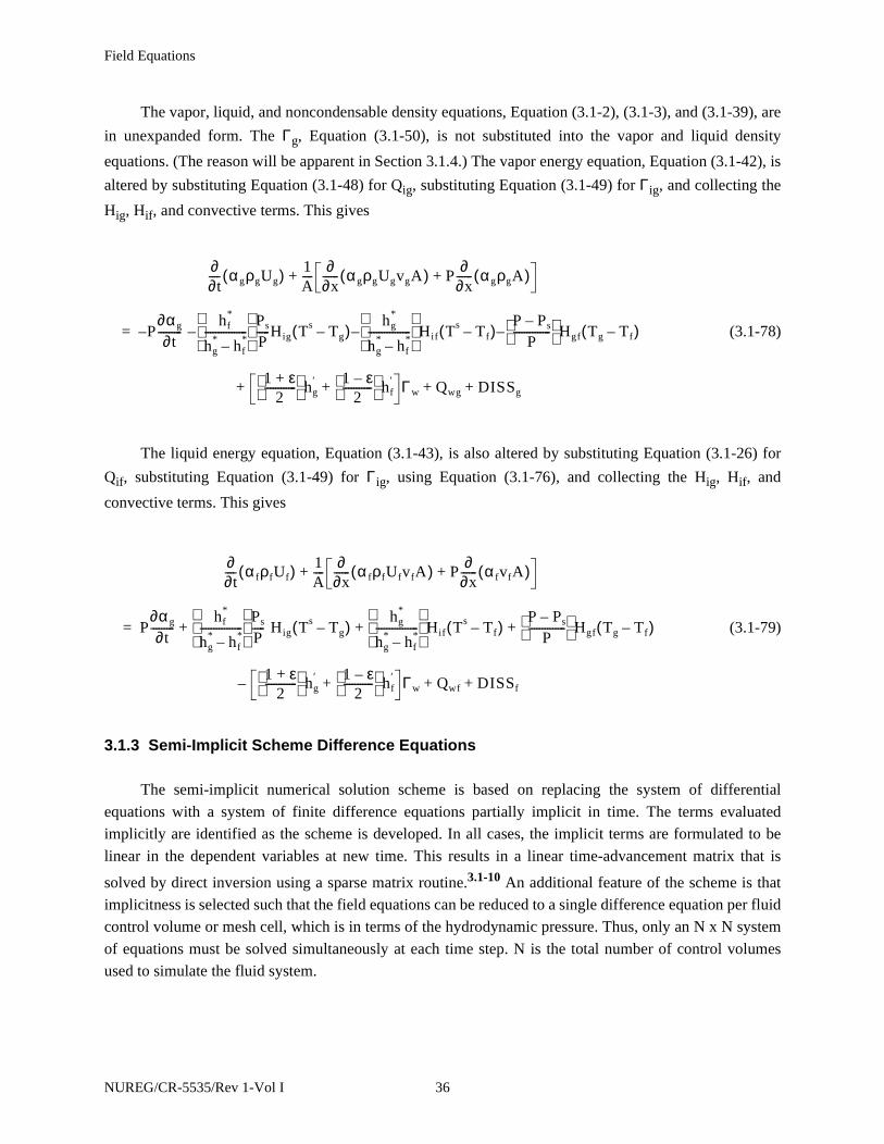
Field Equations
The vapor, liquid, and noncondensable density equations, Equation (3.1-2), (3.1-3), and (3.1-39), are
in unexpanded form. The Γg, Equation (3.1-50), is not substituted into the vapor and liquid density
equations. (The reason will be apparent in Section 3.1.4.) The vapor energy equation, Equation (3.1-42), is
altered by substituting Equation (3.1-48) for Qig, substituting Equation (3.1-49) for Γig, and collecting the
Hig, Hif, and convective terms. This gives
(3.1-78)
The liquid energy equation, Equation (3.1-43), is also altered by substituting Equation (3.1-26) for
Qif, substituting Equation (3.1-49) for Γig, using Equation (3.1-76), and collecting the Hig, Hif, and
convective terms. This gives
(3.1-79)
3.1.3 Semi-Implicit Scheme Difference Equations
The semi-implicit numerical solution scheme is based on replacing the system of differential
equations with a system of finite difference equations partially implicit in time. The terms evaluated
implicitly are identified as the scheme is developed. In all cases, the implicit terms are formulated to be
linear in the dependent variables at new time. This results in a linear time-advancement matrix that is
solved by direct inversion using a sparse matrix routine.3.1-10 An additional feature of the scheme is that
implicitness is selected such that the field equations can be reduced to a single difference equation per fluid
control volume or mesh cell, which is in terms of the hydrodynamic pressure. Thus, only an N x N system
of equations must be solved simultaneously at each time step. N is the total number of control volumes
used to simulate the fluid system.
∂∂t---- αgρgUg( ) 1
A----
∂∂x------ αgρgUgvgA( ) P
∂∂x------ αgρgA( )++
P∂αg
∂t---------–
hf*
hg* hf
*–----------------
Ps
P-----Hig Ts Tg–( )–
hg*
hg* hf
*–----------------
Hif Ts Tf–( )–P P– s
P--------------
– Hgf Tg Tf–( )=
1 ε+2
------------ hg
′ 1 ε–2
----------- hf
′+ Γw Qwg DISSg+ + +
∂∂t---- α fρfUf( ) 1
A----
∂∂x------ α fρfUfvfA( ) P
∂∂x------ α fvfA( )++
P∂α g
∂t---------
hf*
hg* hf
*–----------------
Ps
P----- Hig Ts Tg–( )
hg*
hg* hf
*–----------------
Hif Ts Tf–( )P P– s
P--------------
Hgf Tg Tf–( )+ + +=
1 ε+2
------------ hg
′ 1 ε–2
----------- hf
′+ Γw– Qwf DISSf+ +
NUREG/CR-5535/Rev 1-Vol I 36

Field Equations
It is well known3.1-4,3.1-11 that the system of differential equations constitutes an ill-posed, initial-
value problem. This fact is of little concern physically, since the addition of any second-order differential
effect (regardless of how small), such as viscosity or surface tension, results in a well-posed problem.3.1-12
However, the ill-posedness is of some concern numerically, since it is necessary that the numerical
problem be well-posed. The approximations inherent in any numerical scheme modify the solution
somewhat (truncation error); these effects can be either stabilizing or destabilizing. The resulting
numerical scheme must be stable for mesh sizes of practical interest.
A well-posed and stable numerical algorithm results from employing several stabilizing techniques.
These include the selective implicit evaluation of spatial gradient terms at the new time, donor
formulations for the mass and energy flux terms, and use of a donor-like formulation for the momentum
flux terms. Donor-like formulations for these flux terms are used because of the well-known instability of
an explicit centered finite difference scheme. The term donor-like is used because the momentum flux
formulation consists of a centered formulation for the spatial velocity gradient plus a numerical viscosity
term. These two terms are similar to the form obtained when the momentum flux terms are donored with
the unexpanded form of the momentum equations. The well-posedness of the final numerical scheme, as
well as its accuracy, has been demonstrated for practical cell sizes by extensive numerical testing (see
Volume VI).
The difference equations are based on the concept of a control volume (or mesh cell) in which mass
and energy are conserved by equating accumulation to the rate of mass and energy in through the cell
boundaries minus the rate of mass and energy out through the cell boundaries plus the source terms. This
model results in defining mass and energy volume average properties and requiring knowledge of
velocities at the volume boundaries. The velocities at boundaries are most conveniently defined through
use of momentum control volumes (cells) centered on the mass and energy cell boundaries. This approach
results in a numerical scheme having a staggered spatial mesh. The scalar properties (pressure, energies,
and void fraction) of the flow are defined at cell centers, and vector quantities (velocities) are defined on
the cell boundaries. The resulting one-dimensional spatial noding is illustrated in Figure 3.1-3. The term
cell means an increment in the spatial variable, x, corresponding to the mass and energy control volume.
The difference equations for each cell are obtained by integrating the mass and energy equations
[Equation (3.1-68), (3.1-70), (3.1-71), (3.1-75), and (3.1-77)] with respect to the spatial variable, x, from
the junction at xj to xj+1. The momentum equations [Equation (3.1-72) and (3.1-73)] are integrated with
respect to the spatial variable from cell center to adjoining cell center (xK to xL, Figure 3.1-3). The
equations are listed for the case of a pipe with no branching.
When the mass and energy equations [Equation (3.1-68), (3.1-70), (3.1-71), (3.1-75), and (3.1-77)]
are integrated with respect to the spatial variable from junction j to j+1, differential equations in terms of
cell-average properties and cell boundary fluxes are obtained. The subscripts and superscripts indicate
integration limits for the enclosed quantity.
The sum density Equation (3.1-68) becomes
37 NUREG/CR-5535/Rev 1-Vol I
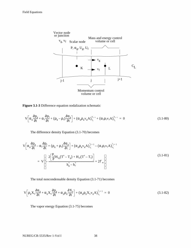
Field Equations
(3.1-80)
The difference density Equation (3.1-70) becomes
(3.1-81)
The total noncondensable density Equation (3.1-71) becomes
(3.1-82)
The vapor energy Equation (3.1-75) becomes
Figure 3.1-3 Difference equation nodalization schematic
Vector node or junction
vg, vf
j-1
K
Mass and energy controlvolume or cell
vg
vf L
j+1
Scalar node
P, αg, Ug, Uf
Momentum controlvolume or cell
j
CL
V α g
∂ρg
∂t-------- α f
∂ρf
∂t-------- ρg ρf–( )
∂αg
∂t---------+ + αgρgvgA( )xj
xj 1+ α fρfvfA( )xj
xj 1++ + 0=
V α g
∂ρg
∂t-------- α f
∂ρf
∂t--------– ρg ρf+( )
∂αg
∂t---------+ α gρgvgA( )xj
j 1+x
α fρfvfA( )xj
j 1+x
–+
V2
Ps
P-----Hig Ts Tg–( ) Hif Ts Tf–( )+
hg* hf
*–--------------------------------------------------------------------------------– 2Γw+
=
V ρgXn
∂α g
∂t--------- αgXn
∂ρg
∂t-------- α gρg
∂Xn
∂t---------+ + αgρgXnvgA( )xj
j 1+x
+ 0=
NUREG/CR-5535/Rev 1-Vol I 38

Field Equations
(3.1-83)
The liquid energy Equation (3.1-77) becomes
(3.1-84)
The sum and difference momentum equations [Equation (3.1-72) and (3.1-73)] are integrated from
cell center to cell center to obtain
(3.1-85)
and
(3.1-86)
V ρgUg P+( )∂αg
∂t--------- αgUg
∂ρg
∂t-------- α gρg
∂Ug
∂t---------+ + α gρgUgvgA( )xj
xj 1+ P α gvgA( )xj
xj 1+++
Vhf
*
hg* hf
*–----------------
Ps
P-----Hig Ts Tg–( )–
hg*
hg* hf
*–----------------
Hif Ts Tf–( )–P P– s
P--------------
– Hgf Tg Tf–( )
=
1 ε+2
------------ hg
′ 1 ε–2
----------- hf
′+ Γw Qwg DISSg }+ + +
V ρfUf P+( )∂αg
∂t---------– α fUf
∂ρf
∂t-------- α fρf
∂Uf
∂t---------+ + α fρfUfvfA( )xj
xj 1+ P α fvfA( )xj
xj 1+++
Vhf
*
hg* hf
*–----------------
Ps
P-----Hig Ts Tg–( )
hg*
hg* hf
*–----------------
Hif Ts Tf–( )P P– s
P--------------
Hgf Tg Tf–( )+ +
=
1 ε+2
------------ hg
′ 1 ε–2
----------- hf
′+– Γw Qwf DISSf }+ +
VA---- αgρg
∂vg
∂t-------- α fρf
∂vf
∂t-------+
12---α gρg vg
2( )xK
xL 12---α fρf vf
2( )xK
xL+ +
P( )xK
xL– ρmBx xL xK–( ) α gρgFWGvg α fρfFWFvf+( ) xL xK–( )–+=
Γ g vg vf–( ) xL xK–( )–
VA----
1Cρm
2
ρgρf----------+
∂vg
∂t--------
∂vf
∂t-------–
12--- vg
2( )xK
xL 12--- vf
2( )xK
xL–+
1ρg-----
1ρf----–
P( )xK
xL– FWGvg FWFvf–( ) xL xK–( )–=
Γ g
ρmvI α fρfvg αgρgvf+( )–α gρgα fρf
------------------------------------------------------------- xL xK–( )+
ρmFI vg vf–( ) xL xK–( )–
ρm
ρgρf----------
ρf ρg–( )By yL yK–( )+
39 NUREG/CR-5535/Rev 1-Vol I
Field Equations
Here, the common area term, A, has been factored from most terms. The quantities shown in brackets
with limits are evaluated at the indicated limits, while the coefficients are averaged over the cell or
integration interval. The indicated derivatives are now derivatives of cell average quantities. Since the
integration interval is centered on the junction, the coefficient averages are approximated by the junction
values. In all cases, the correlation coefficients for averaged products are taken as unity, so averaged
products are replaced directly with products of averages.
Several general guidelines were followed in developing numerical approximations for Equation (3.1-
80) through (3.1-86). These guidelines are summarized below.
• Mass and energy inventories are very important quantities in water reactor safetyanalysis. The numerical scheme should be consistent and conservative in thesequantities. (A greater degree of approximation for momentum effects is consideredacceptable, especially since nuclear reactor flows are dominated by large sources andsinks of momentum ((i.e., pump, abrupt area change). Both mass and energy areconvected from the same cell, and each is evaluated at the same time level; that is, massdensity is evaluated at old time level, so energy density is also evaluated at old time.
• To achieve fast execution speed, implicit evaluation is used only for those termsresponsible for the sonic wave propagation time step limit and those phenomena knownto have small time constants. Thus, implicit evaluation is used for the velocity in themass and energy transport terms, the pressure gradient in the momentum equations, andthe interface mass and momentum exchange terms.
• To further increase computing speed, time-level evaluations are selected so the resultingimplicit terms are linear in the new time variables. Where it is necessary to retainnonlinearities, Taylor series expansions about old time values are used to obtain aformulation linear in the new time variables. (Higher-order terms are neglected.)Linearity results in high computing speed by eliminating the need to iteratively solvesystems of nonlinear equations.
• To allow easy degeneration to homogeneous, or single-phase, formulations, themomentum equations are used as a sum and a difference equation. The particulardifference equation used is obtained by first dividing each of the phasic momentumequations by αgρg and αfρf, for the vapor and liquid phase equations, respectively, and
then subtracting.
Using the above guidelines, the finite difference equations for the mass and energy balances,
corresponding to Equation (3.1-80) through (3.1-84), are listed below. Some of the terms are intermediate
time variables, which are written with a tilde (~). The reason for their use is explained in Section 3.1.4.
The sum continuity equation is
NUREG/CR-5535/Rev 1-Vol I 40
Field Equations
(3.1-87)
The difference continuity equation is
(3.1-88)
The total noncondensable continuity equation is
(3.1-89)
The vapor thermal energy equation is
(3.1-90)
The liquid thermal energy equation is
VL αg L,n ρg L,
n 1+ ρg L,n–( ) α f L,
n ρf L,n 1+ ρf L,
n–( ) ρg L,n ρf L,
n–( ) α g L,n 1+ αg L,
n–( )+ +[ ]
α· g j 1+,n ρ· g j 1+,
nvg j 1+,
n 1+ Aj 1+ α· g j,n ρ· g j,
nvg j,
n 1+ Aj–( )∆t+
α· f j 1+,n ρ· f j 1+,
nvf j 1+,
n 1+ Aj 1+ α· f j,n ρ· f j,
nvf j,
n 1+ Aj–( )∆t+ 0=
VL α g L,n ρg L,
n 1+ ρg L,n–( ) α f L,
n– ρf L,n 1+ ρf L,
n–( ) ρg L,n ρf L,
n+( ) α g L,n 1+ α g L,
n–( )+[ ]
α· g j 1+,n ρ· g j 1+,
nvg j 1+,
n 1+ Aj 1+ α· g j,n ρ· g j,
nvg j,
n 1+ Aj–( )∆t+
α· f j 1+,n ρ· f j 1+,
nvf j 1+,
n 1+ Aj 1+ α· f j,n ρ· f j,
nvf j,
n 1+ Aj–( )– ∆t
2
hg* hf
*–----------------
L
nVL∆t
Ps L,n
PLn
---------Hig L,n TL
s n 1+,Tg L,
n 1+–( ) Hif L,
n TLs n 1+,
Tf L,n 1+
–( )+ 2VL∆tΓw L,n+–=
VL ρg L,n Xn L,
n α g L,n 1+ α g L,
n–( ) αg L,n Xn L,
n ρg L,n 1+ ρg L,
n–( ) α g L,n ρg L,
n Xn L,n 1+
Xn L,n–( )+ +[ ]
α· g j 1+,n ρ· g j 1+,
nX· n j 1+,
nvg j 1+,
n 1+ Aj 1+ α· g j,n ρ· g j,
nX· n j,
nvg j,
n 1+ Aj–( )∆t+ 0=
VL ρg L,n Ug L,
n PLn+( ) αg L,
n 1+ αg L,n–( ) α g L,
n Ug L,n ρg L,
n 1+ ρg L,n–( ) αg L,
n ρg L,n Ug L,
n 1+Ug L,
n–( )+ +[ ]
α· g j 1+,n ρ· g j 1+,
nU· g j 1+,
nPL
n+( )vg j 1+,n 1+ Aj 1+ α· g j,
n ρ· g j,n
U· g j,n
PLn+( )vg j,
n 1+ Aj–[ ]∆ t+
hf*
hg* hf
*–----------------
–
L
nPs L,
n
PL---------Hig L,
n TLs n 1+,
Tg L,n 1+
–( )hg
*
hg* hf
*–----------------
L
n
Hif L,n TL
s n 1+,Tf L,
n 1+–( )–=
–PL
n P– s L,n
PLn
---------------------
Hgf L,n Tg L,
n 1+Tf L,
n 1+–( ) 1 ε+
2------------
hg L,′ n, 1 ε–
2-----------
hf L,′ n,+ Γw L,
n Qwg L,n DISSg L,
n } VL∆t+ + +
41 NUREG/CR-5535/Rev 1-Vol I

Field Equations
(3.1-91)
The quantities having a dot overscore are donored quantities based on the junction velocities, vg,j
and vf,j. The donored quantities are volume average scalar quantities defined analytically as
(3.1-92)
where is any of the donored properties, and vj is the appropriate velocity (that is, vapor or liquid). This
equation holds for the case . For the case vj = 0 and PK > PL,
(3.1-93)
For the case vj = 0 and PK < PL,
(3.1-94)
For the degenerate case vj = 0 and PK = PL, a density-weighted average formulation is used,
(3.1-95)
for all donored properties except for densities (which use a simple average). In this equation, ρK and ρL are
the appropriate densities (e.g., vapor or liquid). Where donored values are not used at junctions, linear
interpolations between neighboring cell values are used. It is not required that and sum to 1; this
can occur in counter-current flow.
VL ρf L,n Uf L,
n PLn+( ) αg L,
n 1+ αg L,n–( )–[ α f L,
n Uf L,n ρf L,
n 1+ ρf L,n–( )+
α f L,n ρf L,
n Uf L,n 1+
Uf L,n–( ) ] α[ ·
f j 1+,n
ρ· f j 1+,n
U· f j 1+,n
PLn+( )vf j 1+,
n 1+ Aj 1++ +
α· f j,n ρ· f j,
nU· f j,
nPL
n+( )vf j,n 1+ Aj ]∆ t–
hf*
hg* hf
*–----------------
L
nPs L,
n
PLn
---------Hig L,n TL
s n 1+,Tg L,
n 1+–( )=
hg*
hg* hf
*–----------------
L
n
Hif L,n TL
s n 1+,Tf L,
n 1+–( )
PLn Ps L,
n–
PLn
------------------
Hgf L,n Tg L,
n 1+Tf L,
n 1+–( )+ +
1 ε+2
------------ hg L,
′ n, 1 ε–2
----------- hf L,
′ n,+ Γw L,n– Qwf L,
n DISSf L,n } VL∆t+ +
φ· j12--- φK φL+( ) 1
2---
vj
vj------- φK φL–( )+=
φ· j
vj 0≠
φ· j φK=
φ· j φL=
φ· jρKφK ρLφL+
ρK ρL+-------------------------------=
α· gj α· fj
NUREG/CR-5535/Rev 1-Vol I 42

Field Equations
The provisional advanced time phasic densities used in Equation (3.1-87) through (3.1-91) are
obtained by linearizing the phasic density state relations about the old time values (see Section 3.2), these
are
(3.1−96)
(3.1−97)
The method of obtaining the phasic density state derivatives used in Equation (3.1-96) and Equation
(3.1-97) is also indicated in Section 3.2.
The provisional advanced time phasic interface heat transfer rates can be written using the finite
difference form of Equation (3.1-48) and (3.1-26) after evaluating the extrapolated temperature ;
these are
(3.1-98)
(3.1-99)
The provisional advanced time temperatures are obtained by linearizing the temperature state
relations about the old time values (see Section 3.2). These are
(3.1-100)
(3.1-101)
(3.1-102)
The method used in Equation (3.1-100) through (3.1-102) to obtain the temperature state derivatives
is also indicated in Section 3.2.
ρg L,n 1+ ρg L,
n ∂ρg
∂P--------
L
n
PLn 1+ PL
n–( )∂ρg
∂Xn---------
L
n
Xn L,n 1+
Xn L,n–( )
∂ρg
∂Ug---------
L
n
Ug L,n 1+
Ug L,n–( )+ + +=
ρf L,n 1+ ρf L,
n ∂ρf
∂P--------
L
n
PLn 1+ PL
n–( )∂ρf
∂Uf---------
L
n
Uf L,n 1+
Uf L,n–( )+ +=
Tn 1+
Qig L,n 1+ Ps L,
n
PLn
---------Hig L,n TL
s n 1+,Tg L,
n 1+–( ) 1 ε–
2-----------
Γw L,n hg L,
′ n, hf L,′ n,–( )–=
Qif L,n 1+
Hif L,n TL
s n 1+,Tf L,
n 1+–( ) 1 ε+
2------------
Γw L,n hg L,
′ n, hf L,′ n,–( )–=
TLs n 1+,
TLs n, ∂Ts
∂P--------
L
n
PLn 1+ PL
n–( ) ∂Ts
∂Xn---------
L
n
Xn L,n 1+
Xn L,n–( ) ∂Ts
∂Ug---------
L
n
Ug L,n 1+
Ug L,n–( )+ + +=
Tg L,n 1+
Tg L,n ∂Tg
∂P---------
L
n
PLn 1+ PL
n–( )∂Tg
∂Xn---------
L
n
Xn L,n 1+
Xn L,n–( )
∂Tg
∂Ug---------
L
n
Ug L,n 1+
Ug L,n–( )+ + +=
Tf L,n 1+
Tf L,n ∂Tf
∂P--------
L
n
PLn 1+ PL
n–( )∂Tf
∂Uf---------
L
n
Uf L,n 1+
Uf L,n–( )+ +=
43 NUREG/CR-5535/Rev 1-Vol I
Field Equations
The previously stated guidelines are also used to obtain the finite-difference equations for the phasic
momentum equations. In this case, volume-average properties for the momentum control volume are taken
as junction properties (that is, linear interpolations between mass and energy control volume centers). The
momentum flux terms are approximated using a donor-like formulation that results in a centered velocity
gradient term and a viscous-like term (artificial viscosity). The finite difference equations for the sum and
difference momentum equations, Equation (3.1-85) and (3.1-86), are
(3.1-103)
(3.1-104)
where the so-called viscous terms are defined as
(3.1-105)
αgρg( )jn vg
n 1+ vgn–( )j∆xj α fρf( )j
n vfn 1+ vf
n–( )j∆xj+
12--- α· gρ· g( )j
nvg
2( )Ln
vg2( )K
n–[ ]∆ t
12--- α· fρ· f( )j
nvf
2( )Ln
vf2( )K
n–[ ]∆ t+ +
12--- α· gρ· g( )j
nVISGj
n α· fρ· f( )jnVISFj
n+[ ]∆ t–
PL PK–( )n 1+ ∆t– ρm( )jn[ Bx αgρg( )j
nFWGjn vg( )j
n 1+–+=
α fρf( )jnFWFj
n vf( )jn 1+– Γ g( )j
n vg vf–( )jn 1+ ]∆xj∆t–
α· gρ· g( )jnHLOSSGj
nvg j,n 1+ α· fρ· f( )j
nHLOSSFj
nvf j,n 1++[ ]∆ t–
1Cρm
2
ρgρf----------+
j
n
vgn 1+ vg
n–( ) vfn 1+ vf
n–( )–[ ] j∆xj
12---
α· gρ· g
αgρg-----------
j
n
vg2( )L
nvg
2( )Kn
–[ ]∆ t12---
α· gρ· g
αgρg-----------
j
n
VISGjn∆t–+
12---
α· fρ· f
α fρf----------
j
n
vf2( )L
nvf
2( )Kn
–[ ]∆ t–12---
α· fρ· f
α fρf----------
j
n
VISFjn∆t
ρf ρ– g
ρgρf-------------
j
n
PL PK–( )n 1+ ∆t–=+
FWGjn vg( )j
n 1+ FWFjn vf( )j
n 1+ Γ gn ρm
n vIn 1+ α f
nρfnvg
n 1+– αgnρg
nvfn 1+–( )
αgρgα fρf( )n---------------------------------------------------------------------------------------
j
––
–
ρmFI( )jn vg
n 1+( vfn 1+ )j– }∆ xj∆t
α· gρ· g
αgρg-----------
j
n
HLOSSGjnvg j,
n 1+–+
α· fρ· f
α fρf----------
j
n
HLOSSFjnvf j,
n 1+ ]∆ t–
ρm
ρgρf----------
j
n
ρf ρg–( )jnBy yL
n yKn–( )∆t+
VISGjn 1
2--- vg L,
n vgn( )j 1+
Aj 1+
Aj----------- vg
n( )j– vg K,n vg
n( )j vgn( )j 1–
Aj 1–
Aj-----------––
=
NUREG/CR-5535/Rev 1-Vol I 44
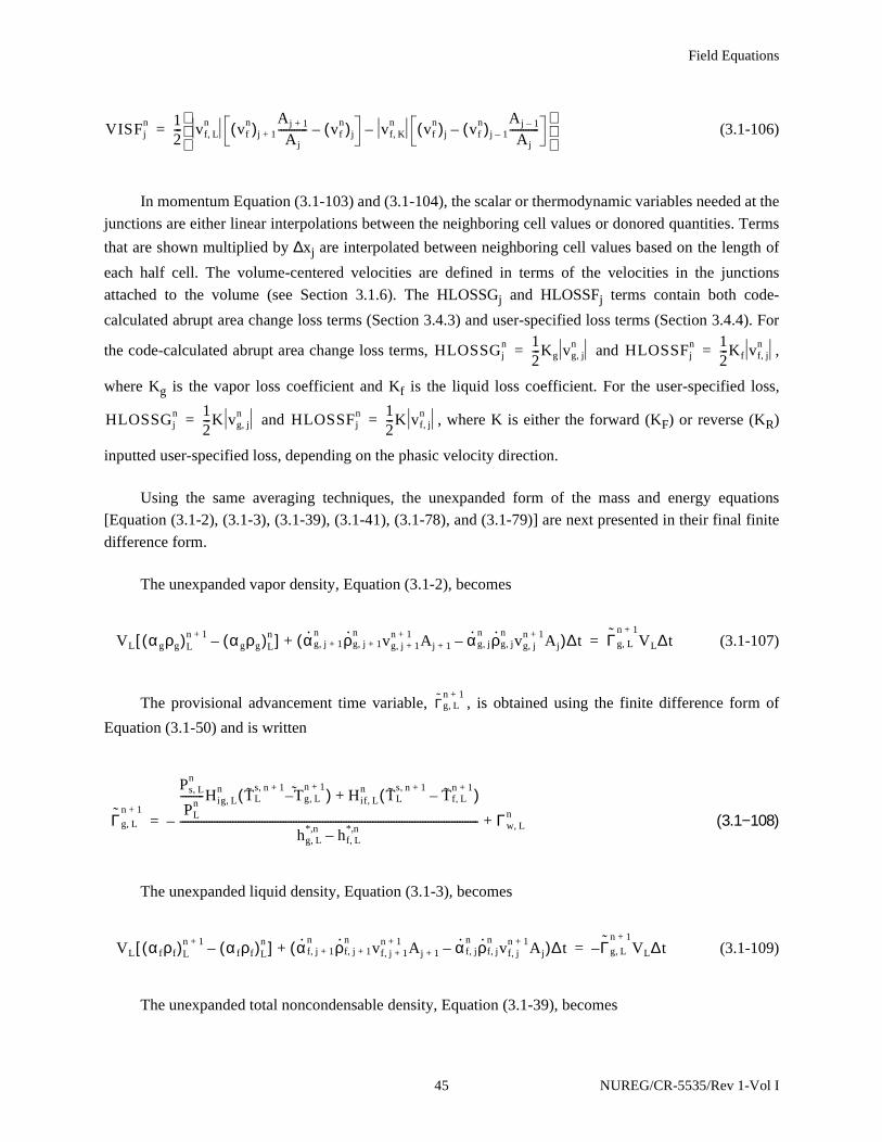
Field Equations
(3.1-106)
In momentum Equation (3.1-103) and (3.1-104), the scalar or thermodynamic variables needed at the
junctions are either linear interpolations between the neighboring cell values or donored quantities. Terms
that are shown multiplied by ∆xj are interpolated between neighboring cell values based on the length of
each half cell. The volume-centered velocities are defined in terms of the velocities in the junctions
attached to the volume (see Section 3.1.6). The HLOSSGj and HLOSSFj terms contain both code-
calculated abrupt area change loss terms (Section 3.4.3) and user-specified loss terms (Section 3.4.4). For
the code-calculated abrupt area change loss terms, and ,
where Kg is the vapor loss coefficient and Kf is the liquid loss coefficient. For the user-specified loss,
and , where K is either the forward (KF) or reverse (KR)
inputted user-specified loss, depending on the phasic velocity direction.
Using the same averaging techniques, the unexpanded form of the mass and energy equations
[Equation (3.1-2), (3.1-3), (3.1-39), (3.1-41), (3.1-78), and (3.1-79)] are next presented in their final finite
difference form.
The unexpanded vapor density, Equation (3.1-2), becomes
(3.1-107)
The provisional advancement time variable, , is obtained using the finite difference form of
Equation (3.1-50) and is written
(3.1−108)
The unexpanded liquid density, Equation (3.1-3), becomes
(3.1-109)
The unexpanded total noncondensable density, Equation (3.1-39), becomes
VISFjn 1
2--- vf L,
n vfn( )j 1+
Aj 1+
Aj----------- vf
n( )j– vf K,n vf
n( )j vfn( )j 1–
Aj 1–
Aj-----------––
=
HLOSSGjn 1
2---Kg vg j,
n= HLOSSFjn 1
2---Kf vf j,
n=
HLOSSGjn 1
2---K vg j,
n= HLOSSFjn 1
2---K vf j,
n=
VL αgρg( )Ln 1+ αgρg( )L
n–[ ] α· g j 1+,n ρ· g j 1+,
nvg j 1+,
n 1+ Aj 1+ α· g j,n ρ· g j,
nvg j,
n 1+ Aj–( )∆t+ Γ g L,n 1+
VL∆t=
Γg L,n 1+
Γ g L,n 1+
Ps L,n
PLn
---------Hig L,n TL
s n 1+,T– g L,
n 1+( ) Hif L,
n TLs n 1+,
Tf L,n 1+
–( )+
hg L,*,n hf L,
*,n –-----------------------------------------------------------------------------------------------------------------– Γw L,
n+=
VL α fρf( )Ln 1+ α fρf( )L
n–[ ] α· f j 1+,n ρ· f j 1+,
nvf j 1+,
n 1+ Aj 1+ α· f j,n ρ· f j,
nvf j,
n 1+ Aj–( )∆t+ Γg L,n 1+
VL∆t–=
45 NUREG/CR-5535/Rev 1-Vol I
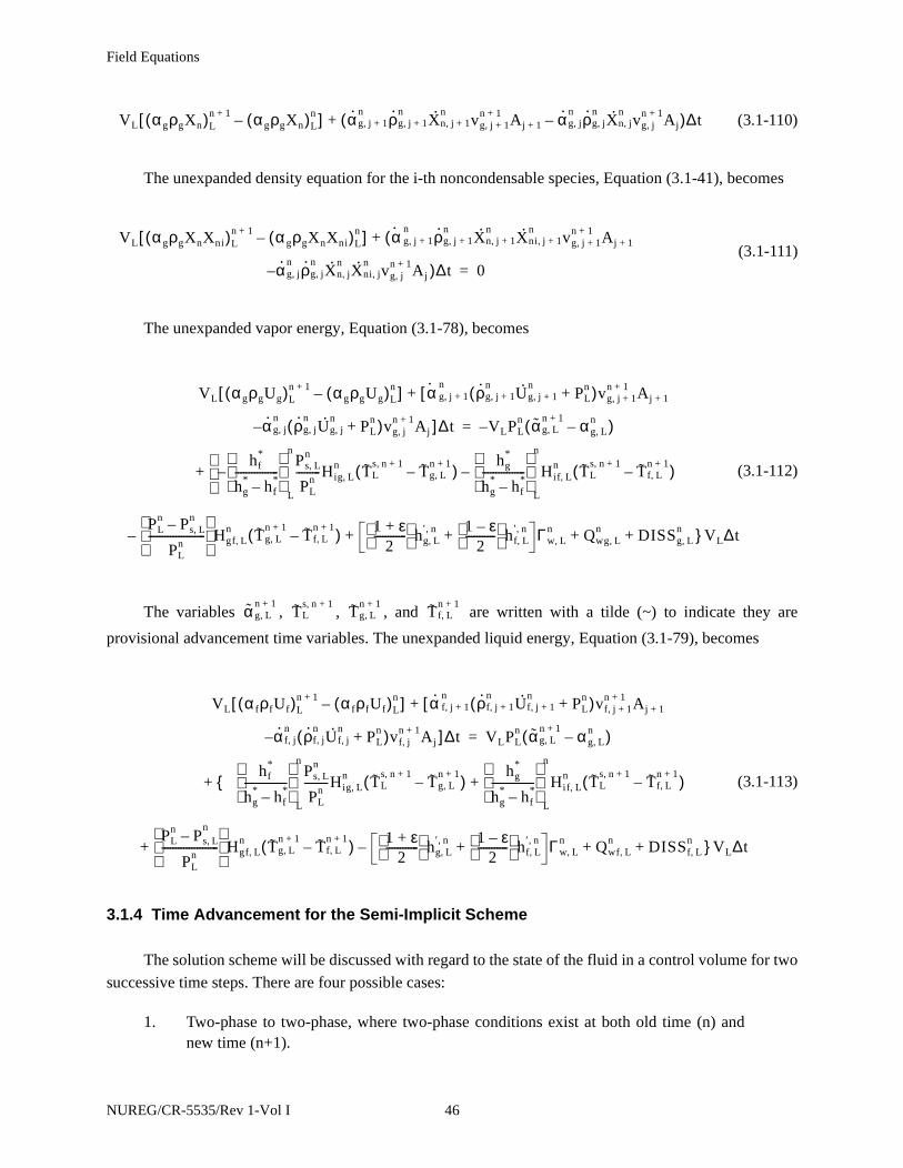
Field Equations
(3.1-110)
The unexpanded density equation for the i-th noncondensable species, Equation (3.1-41), becomes
(3.1-111)
The unexpanded vapor energy, Equation (3.1-78), becomes
(3.1-112)
The variables , , , and are written with a tilde (~) to indicate they are
provisional advancement time variables. The unexpanded liquid energy, Equation (3.1-79), becomes
(3.1-113)
3.1.4 Time Advancement for the Semi-Implicit Scheme
The solution scheme will be discussed with regard to the state of the fluid in a control volume for two
successive time steps. There are four possible cases:
1. Two-phase to two-phase, where two-phase conditions exist at both old time (n) andnew time (n+1).
VL αgρgXn( )Ln 1+ αgρgXn( )L
n–[ ] α· g j 1+,n ρ· g j 1+,
nX· n j 1+,
nvg j 1+,
n 1+ Aj 1+ α· g j,n ρ· g j,
nX· n j,
nvg j,
n 1+ Aj–( )∆t+
VL αgρgXnXni( )Ln 1+ α gρgXnXni( )L
n–[ ] α( ·g j 1+,n
ρ· g j 1+,n
X· n j 1+,n
X· ni j 1+,n
vg j 1+,n 1+ Aj 1++
α· g j,n ρ· g j,
nX· n j,
nX· ni j,
nvg j,
n 1+ Aj )∆t– 0=
VL αgρgUg( )Ln 1+ αgρgUg( )L
n–[ ] α[ ·g j 1+,n
ρ· g j 1+,n
U· g j 1+,n
PLn+( )vg j 1+,
n 1+ Aj 1++
α· g j,n ρ· g j,
nU· g j,
nPL
n+( )vg j,n 1+ Aj ]∆ t– VLPL
n αg L,n 1+ αg L,
n–( )–=
hf*
hg* hf
*–----------------
–
L
nPs L,
n
PLn
---------Hig L,n TL
s n 1+,Tg L,
n 1+–( )
hg*
hg* hf
*–----------------
L
n
Hif L,n TL
s n 1+,Tf L,
n 1+–( )–+
PLn Ps L,
n–
PLn
---------------------
Hgf L,n Tg L,
n 1+Tf L,
n 1+–( )–
1 ε+2
------------ hg L,
′ n, 1 ε–2
----------- hf L,
′ n,+ Γw L,n Qwg L,
n DISSg L,n } VL∆t+ + +
α g L,n 1+
TLs n 1+,
Tg L,n 1+
Tf L,n 1+
VL α fρfUf( )Ln 1+ α fρfUf( )L
n–[ ] α·[ f j 1+,n ρ· f j 1+,
nU· f j 1+,
nPL
n+( )vf j 1+,n 1+ Aj 1++
α· f j,n ρ· f j,
nU· f j,
nPL
n+( )vf j,n 1+ Aj ]∆ t– VLPL
n αg L,n 1+ αg L,
n–( )=
{+hf
*
hg* hf
*–----------------
L
nPs L,
n
PLn
---------Hig L,n TL
s n 1+,Tg L,
n 1+–( )
hg*
hg* hf
*–----------------
L
n
Hif L,n TL
s n 1+,Tf L,
n 1+–( )+
PLn P– s L,
n
PLn
---------------------
Hgf L,n Tg L,
n 1+Tf L,
n 1+–( ) 1 ε+
2------------
hg L,′ n, 1 ε–
2-----------
hf L,′ n,+ Γw L,
n– Qwf L,n DISSf L,
n } VL∆t+ + +
NUREG/CR-5535/Rev 1-Vol I 46

Field Equations
2. One-phase to one-phase, where one-phase conditions (either pure gas or pure liquid)exist at both old time (n) and new time (n+1).
3. Two-phase to one-phase (disappearance), where two-phase conditions exist at oldtime (n), and one-phase conditions exist at new time (n+1).
4. One-phase to two-phase (appearance), where one-phase conditions exist at old time(n), and two-phase conditions exist at new time (n+1).
The solution scheme will first be presented for the two-phase to two-phase case, because it is the
most general. The solution scheme for the other three cases will then be presented.
3.1.4.1 Two-Phase To Two-Phase.
First, the density and temperature Equation (3.1-96), (3.1-97), (3.1-100), (3.1-101) and (3.1-102) are
substituted into the five expanded density and energy difference Equation (3.1-87) through (3.1-91). The
equations are then ordered so that the noncondensable density equation is first, the vapor energy equation
is second, the liquid energy equation is third, the difference density equation is fourth, and the sum density
equation is fifth. The five density and energy variables are expressed as differences, and the order is
(3.1-114)
The tilde (~) is used for Xn, Ug, Uf, and αg to indicate that these are provisional new time variables
and do not represent the final new time variables for the two-phase to two-phase case. The ordering of the
variables and equations was selected so that a given equation is dominated by its corresponding variable
(e.g., the vapor energy equation is second and the vapor energy variable Ug is also second). The
noncondensable equation is placed first for ease of degeneration when a noncondensable component is not
specified in the problem, and the pressure variable is placed last for numerical convenience in the pressure
solution. The five equations are then each divided by the volume VL. The system of equations has the
following form, where the matrix and the vectors contain only old time level variables
(the subscript L and the superscript n has been dropped for the listing of the matrix and vectors):
(3.1-115)
where
Xn L,n 1+
Xn L,n–( ) Ug L,
n 1+Ug L,
n–( ) Uf L,n 1+
Uf L,n–( ) αg L,
n 1+ αg L,n–( ) PL
n 1+ PLn–( ), , , ,
A˜
b˜
g˜
1 g˜
2 f˜
1 f˜
2, , , ,
A˜
x˜
b˜
g˜
1vg j 1+,n 1+ g
˜
2vg j,n 1+ f
˜
1vf j 1+,n 1+ f
˜
2vf j,n 1++ + + +=
47 NUREG/CR-5535/Rev 1-Vol I

Field Equations
= (3.1-116)
= (3.1-117)
A11 = (3.1-118)
A12 = (3.1-119)
A14 = ρgXn (3.1-120)
A15 = (3.1-121)
A21 = (3.1-122)
A22 = (3.1-123)
A˜
A11 A12 0 A14 A15
A21 A22 A23 A24 A25
A31 A32 A33 A34 A35
A41 A42 A43 A44 A45
A51 A52 A53 A54 A55
x˜
Xn L,n 1+
Xn L,n–
Ug L,n 1+
Ug L,n–
Uf L,n 1+
Uf L,n–
αg L,n 1+ αg L,
n–
PLn 1+ PL
n–
=
b˜
0
b2
b3
b4
0
g˜
1
g11
g21
0
g41
g51
= g˜
2
g12
g22
0
g42
g52
= f˜
1
0
0
f31
f41
f51
= f˜
2
0
0
f32
f42
f52
=
α g Xn Xn∂∂ρg ρg+
α gXn Ug∂∂ρg
α gXn P∂∂ρg
αgUg Xn∂∂ρg hf
*
hg* hf
*–----------------
∆tPs
P-----Hig Xn∂
∂Ts
Xn∂∂Tg–
+
hg*
hg* hf
*–----------------
+ ∆tHif Xn∂∂Ts
∆tP P– s
P--------------
Hgf Xn∂∂Tg+
αg Ug Ug∂∂ρg ρg+
hf*
hg* hf
*–----------------
∆tPs
P-----Hig Ug∂
∂Ts
Ug∂∂Tg–
+
+hg
*
hg* hf
*–----------------
∆tHif Ug∂∂Ts
∆tP P– s
P--------------
Hgf Ug∂∂Tg+
NUREG/CR-5535/Rev 1-Vol I 48

Field Equations
A23 = (3.1-124)
A24 = ρgUg + P (3.1-125)
A25 = (3.1-126)
A31 = (3.1-127)
A32 = (3.1-128)
A33 = (3.1-129)
A34 = - ρfUf - P (3.1-130)
A35 = (3.1-131)
A41 = (3.1-132)
hg*
hg* hf
*–----------------
– ∆tHif Uf∂∂Tf ∆t
P P– s
P--------------
Hgf Uf∂∂Tf–
αgUg P∂∂ρg hf
*
hg* hf
*–----------------
∆tPs
P-----Hig P∂
∂Ts
P∂∂Tg–
+
hg*
hg* hf
*–----------------
∆tHif P∂∂Ts
P∂∂Tf–
∆tP P– s
P--------------
Hgf P∂∂Tg
P∂∂Tf–
+ +
hf*
hg* hf
*–----------------
∆tPs
P-----Hig Xn∂
∂Ts
Xn∂∂Tg–
–hg
*
hg* hf
*–----------------
∆tHif∂Ts
∂Xn---------–
∆tP P– s
P--------------
Hgf
∂Tg
∂Xn---------–
hf*
hg* hf
*–----------------
∆tPs
P-----Hig Ug∂
∂Ts
Ug∂∂Tg–
hg*
hg* hf
*–----------------
∆tHif Ug∂∂Ts
––
∆tP P– s
P--------------
Hgf Ug∂∂Tg–
α f Uf Uf∂∂ρf ρf+
hg*
hg* hf
*–----------------
∆tHif Uf∂∂Tf ∆t
P P– s
P--------------
Hgf Uf∂∂Tf+ +
α fUf P∂∂ρf hf
*
hg* hf
*–----------------
∆tPs
P-----Hig P∂
∂Ts
P∂∂Tg–
–
hg*
hg* hf
*–----------------
– ∆tHif P∂∂Ts
P∂∂Tf–
∆tP P– s
P--------------
Hgf P∂∂Tg
P∂∂Tf–
–
α g Xn∂∂ρg 2
hg* hf
*–----------------
∆tPs
P-----Hig Xn∂
∂Ts
Xn∂∂Tg–
2
hg* hf
*–----------------
∆tHif Xn∂∂Ts
+ +
49 NUREG/CR-5535/Rev 1-Vol I
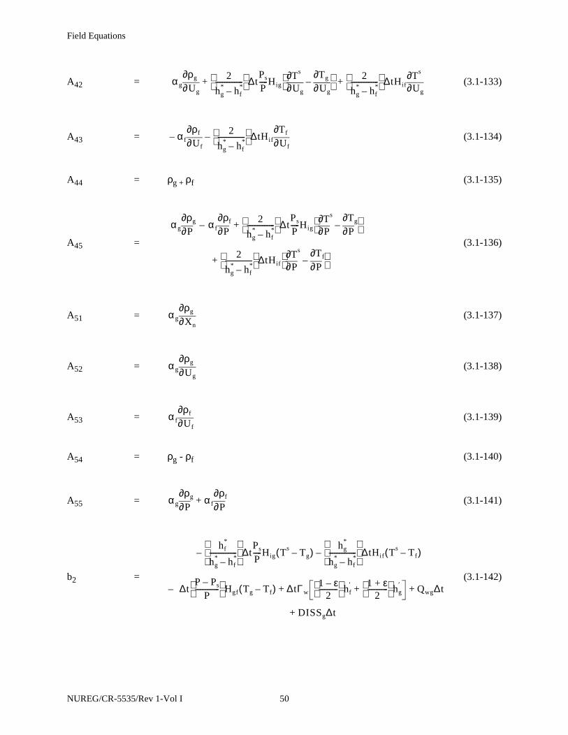
Field Equations
A42 = (3.1-133)
A43 = (3.1-134)
A44 = ρg + ρf (3.1-135)
A45 = (3.1-136)
A51 = (3.1-137)
A52 = (3.1-138)
A53 = (3.1-139)
A54 = ρg - ρf (3.1-140)
A55 = (3.1-141)
b2 = (3.1-142)
α g Ug∂∂ρg 2
hg* hf
*–----------------
∆tPs
P-----Hig Ug∂
∂Ts
Ug∂∂Tg–
+2
hg* hf
*–----------------
∆tHif Ug∂∂Ts
+
α f Uf∂∂ρf–
2
hg* hf
*–----------------
∆tHif Uf∂∂Tf–
α g P∂∂ρg α f–
P∂∂ρf 2
hg* hf
*–----------------
∆tPs
P-----Hig P∂
∂Ts
P∂∂Tg–
+
2
hg* hf
*–----------------
∆tHif P∂∂Ts
P∂∂Tf–
+
α g Xn∂∂ρg
α g Ug∂∂ρg
α f Uf∂∂ρf
α g P∂∂ρg α f P∂
∂ρf+
hf*
hg* hf
*–----------------
∆tPs
P-----Hig Ts Tg–( )–
hg*
hg* hf
*–----------------
∆tHif Ts Tf–( )–
– ∆tP P– s
P--------------
Hgf Tg Tf–( ) ∆tΓw1 ε–
2-----------
hf′ 1 ε+
2------------
hg′+ Qwg∆t+ +
D+ ISSg∆t
NUREG/CR-5535/Rev 1-Vol I 50
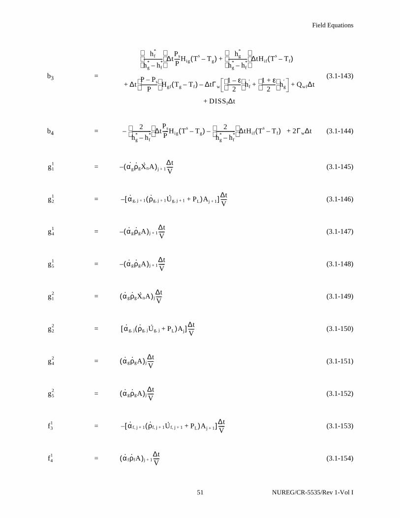
Field Equations
b3 = (3.1-143)
b4 = (3.1-144)
= (3.1-145)
= (3.1-146)
= (3.1-147)
= (3.1-148)
= (3.1-149)
= (3.1-150)
= (3.1-151)
= (3.1-152)
= (3.1-153)
= (3.1-154)
hf*
hg* hf
*–----------------
∆tPs
P-----Hig Ts Tg–( )
hg*
hg* hf
*–----------------
∆tHif Ts Tf–( )+
∆+ tP P– s
P--------------
Hgf Tg Tf–( ) ∆tΓw1 ε–
2-----------
hf′ 1 ε+
2------------
hg′+– Qwf∆t+
DISSf∆t+
2
hg* hf
*–----------------
∆tPs
P-----Hig Ts Tg–( )–
2
hg* hf
*–----------------
∆tHif Ts Tf–( ) 2+ Γw∆t–
g11 αg
· ρ· gX· nA( )j 1+∆tV-----–
g21 α· g j 1+, ρ· g j 1+, U· g j 1+, PL+( )Aj 1+[ ] ∆t
V-----–
g41 α· gρ· gA( )j 1+
∆tV-----–
g51 α· gρ· gA( )j 1+
∆tV-----–
g12 α· gρ· gX· nA( )j
∆tV-----
g22 α· g j, ρ· g j, U· g j, PL+( )Aj[ ] ∆t
V-----
g42 α· gρ· gA( )j
∆tV-----
g52 α· gρ· gA( )j
∆tV-----
f31 α· f j 1+, ρ· f j 1+, U· f j 1+, PL+( )Aj 1+[ ]–
∆tV-----
f41 α· fρ· fA( )j 1+
∆tV-----
51 NUREG/CR-5535/Rev 1-Vol I
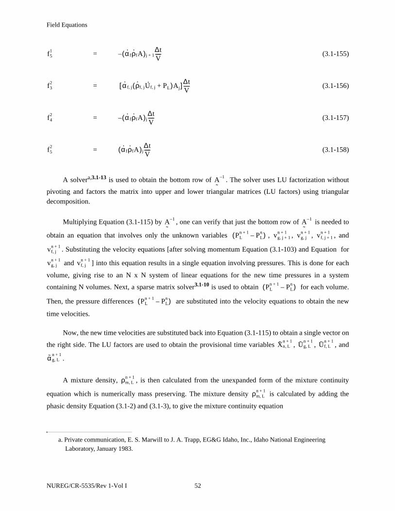
Field Equations
= (3.1-155)
= (3.1-156)
= (3.1-157)
= (3.1-158)
A solvera,3.1-13 is used to obtain the bottom row of . The solver uses LU factorization without
pivoting and factors the matrix into upper and lower triangular matrices (LU factors) using triangular
decomposition.
Multiplying Equation (3.1-115) by , one can verify that just the bottom row of is needed to
obtain an equation that involves only the unknown variables , , , , and
. Substituting the velocity equations [after solving momentum Equation (3.1-103) and Equation for
and ] into this equation results in a single equation involving pressures. This is done for each
volume, giving rise to an N x N system of linear equations for the new time pressures in a system
containing N volumes. Next, a sparse matrix solver3.1-10 is used to obtain for each volume.
Then, the pressure differences are substituted into the velocity equations to obtain the new
time velocities.
Now, the new time velocities are substituted back into Equation (3.1-115) to obtain a single vector on
the right side. The LU factors are used to obtain the provisional time variables , , , and
.
A mixture density, , is then calculated from the unexpanded form of the mixture continuity
equation which is numerically mass preserving. The mixture density is calculated by adding the
phasic density Equation (3.1-2) and (3.1-3), to give the mixture continuity equation
a. Private communication, E. S. Marwill to J. A. Trapp, EG&G Idaho, Inc., Idaho National Engineering
Laboratory, January 1983.
f51 α· fρ· fA( )j 1+–
∆tV-----
f32 α· f j, ρ· f j, U· f j, PL+( )Aj[ ] ∆t
V-----
f42 α· fρ· fA( )j–
∆tV-----
f52 α· fρ· fA( )j
∆tV-----
A˜
1–
A˜
1– A˜
1–
PLn 1+ PL
n–( ) vg j 1+,n 1+ vg j,
n 1+ vf j 1+,n 1+
vf j,n 1+
vg j,n 1+ vf j,
n 1+
PLn 1+ PL
n–( )
PLn 1+ PL
n–( )
Xn L,n 1+
Ug L,n 1+
Uf L,n 1+
α g L,n 1+
ρm L,n 1+
ρm L,n 1+
NUREG/CR-5535/Rev 1-Vol I 52

Field Equations
(3.1-159)
The mass-preserving finite difference approximation is
(3.1-160)
from which is obtained. The density is compared with the mixture density, , which is
calculated from the state relations. The difference between these two mixture densities is used to provide a
time step control based on truncation in the calculation of the mixture density (see Section 8.1).
Next, is calculated using Equation (3.1-108), where , , and are obtained
from Equation (3.1-100) through (3.1-102) using the newly calculated variables , , , and
.
To obtain the new time variables , , , , and , the unexpanded difference
equations, Equation (3.1-107), (3.1-109), (3.1-110), (3.1-111), (3.1-112), and (3.1-113), are used. In the
discussion introducing the unexpanded difference equations, motives were given for use of the
unexpanded form. Extensive numerical testing has shown the benefits of the following procedures.
Using the phasic convective terms along with from Equation (3.1-108), the unexpanded phasic
density Equation (3.1-107) and (3.1-109) are used to obtain and .
Next, the unexpanded total noncondensable density Equation (3.1-110) is used to calculate
, which is then divided by to obtain .
The unexpanded individual noncondensable density Equation (3.1-111) is then used to calculate
, which is divided by to obtain .
Following this, the unexpanded vapor energy Equation (3.1-112) is used with the vapor energy
source and convective terms from the expanded equation as well as the provisional time variables ,
, and to obtain , which is divided by to give . Analogously, the
unexpanded liquid energy Equation (3.1-113) is used to obtain , which is divided by
to give .
∂ρm
∂t---------
1A----
x∂∂ α gρgvgA α fρfvfA+( )+ 0=
VL ρm L,n 1+ ρL
n–( ) α· g j 1+,n ρ· g j 1+,
nvg j 1+,
n 1+ Aj 1+ α· g j,n ρ· g j,
nvg j,
n 1+ Aj–( )∆t+
α· f j 1+,n ρ· f j 1+,
nvf j 1+,
n 1+ Aj 1+ α· f j,n ρ· f j,
nvf j,
n 1+ Aj–( )+ ∆t 0=
ρm L,n 1+ ρm L,
n 1+ ρLn 1+
Γ g L,n 1+
TLs n 1+,
Tg L,n 1+
Tf L,n 1+
PLn 1+ Ug L,
n 1+Uf L,
n 1+
Xn L,n 1+
Xn L,n 1+ Xni L,
n 1+ Ug L,n 1+ Uf L,
n 1+ αg L,n 1+
Γg L,n 1+
α gρg( )Ln 1+ α fρf( )L
n 1+
αgρgXn( )Ln 1+ α gρg( )L
n 1+ Xn L,n 1+
αgρgXnXni( )Ln 1+ αgρgXn( )L
n 1+ Xni L,n 1+
Ts n 1+,
Tgn 1+
Tfn 1+ αgρgUg( )L
n 1+ α gρg( )Ln 1+ Ug L,
n 1+
α fρfUf( )Ln 1+
α fρf( )Ln 1+ Uf L,
n 1+
53 NUREG/CR-5535/Rev 1-Vol I
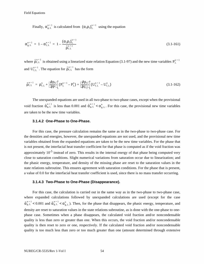
Field Equations
Finally, is calculated from using the equation
(3.1-161)
where is obtained using a linearized state relation Equation (3.1-97) and the new time variables
and . The equation for has the form
(3.1-162)
The unexpanded equations are used in all two-phase to two-phase cases, except when the provisional
void fraction is less than 0.001 and . For this case, the provisional new time variables
are taken to be the new time variables.
3.1.4.2 One-Phase to One-Phase.
For this case, the pressure calculation remains the same as in the two-phase to two-phase case. For
the densities and energies, however, the unexpanded equations are not used, and the provisional new time
variables obtained from the expanded equations are taken to be the new time variables. For the phase that
is not present, the interfacial heat transfer coefficient for that phase is computed as if the void fraction was
approximately 10-5 instead of zero. This results in the internal energy of that phase being computed very
close to saturation conditions. Slight numerical variations from saturation occur due to linearization; and
the phasic energy, temperature, and density of the missing phase are reset to the saturation values in the
state relations subroutine. This ensures agreement with saturation conditions. For the phase that is present,
a value of 0.0 for the interfacial heat transfer coefficient is used, since there is no mass transfer occurring.
3.1.4.3 Two-Phase to One-Phase (Disappearance).
For this case, the calculation is carried out in the same way as in the two-phase to two-phase case,
where expanded calculations followed by unexpanded calculations are used (except for the case
). Then, for the phase that disappears, the phasic energy, temperature, and
density are reset to saturation values in the state relations subroutine, as is done with the one-phase to one-
phase case. Sometimes when a phase disappears, the calculated void fraction and/or noncondensable
quality is less than zero or greater than one. When this occurs, the void fraction and/or noncondensable
quality is then reset to zero or one, respectively. If the calculated void fraction and/or noncondensable
quality is too much less than zero or too much greater than one (amount determined through extensive
αg L,n 1+ α fρf( )L
n 1+
αg L,n 1+ 1 α f L,
n 1+– 1α fρf( )L
n 1+
ρf L,n 1+
-----------------------–= =
ρf L,n 1+
PLn 1+
Uf L,n 1+ ρf L,
n 1+
ρf L,n 1+ ρf L,
n ∂ρf
∂P--------
L
n
PLn 1+ PL
n–( )∂ρf
∂Uf---------
L
n
Uf L,n 1+ Uf L,
n–( )+ +=
αg L,n 1+ α g L,
n 1+ αg L,n<
α g L,n 1+
0.001 and < αg L,n 1+ αg L,
n<
NUREG/CR-5535/Rev 1-Vol I 54
Field Equations
testing, which is consistent with the mass error check), an error is assumed to have occurred, and the time
step is reduced and repeated.
3.1.4.4 One-Phase to Two-Phase (Appearance).
Here, the calculation proceeds in the same way as in the one-phase to one-phase case. For the phase
that is not present, the large interfacial heat transfer coefficient for that phase is computed as if the void
fraction was approximately 10-5 instead of zero. This results in the energy and temperature of that phase
being computed very close to saturation conditions. Because the phase that is appearing is assumed to
appear at saturation conditions, an error can be made if, in reality, the phase appeared by convection from
a neighboring volume that was at a temperature different from saturation. The magnitude of the potential
error is controlled by letting the phase appear at saturation but restricting the amount that can appear by
time step control. If more than the limiting amount (amount determined through extensive testing) appears,
an error is assumed to have occurred, and the time step is reduced and repeated.
3.1.5 Difference Equations and Time Advancement for the Nearly-Implicit Scheme
For problems where the flow is expected to change very slowly with time, it is possible to obtain
adequate information from an approximate solution based on very large time steps. This would be
advantageous if a reliable and efficient means could be found for solving difference equations treating all
terms (i.e., phase exchanges, pressure propagation, and convection) by implicit differences. Unfortunately,
the state of the art is less satisfactory here than in the case of semi-implicit (convection-explicit) schemes.
For illustration, a fully implicit scheme for the six-equation model of a 100-volume problem would require
the solution of 600 coupled algebraic equations. If these equations were linearized for a pipe with no
branching, inversion of a block tri-diagonal, 600 x 600 matrix with 6 x 6 blocks would be required. This
would yield a matrix of bandwidth 23 containing ~13,800 nonzero elements, resulting in an extremely
costly time-advancement scheme. Note that the tri-diagonal shape is limited to a pipe with no branching
problem.
To reduce the number of calculations required for solving fully implicit difference schemes,
fractional step (sometimes called multiple step) methods have been tried. The equations can be split into
fractional steps based upon physical phenomena. This is the basic idea in the nearly-implicit scheme.
Fractional step methods for two-phase flow problems have been developed.3.1-14,3.1-15 These earlier
efforts have been used to guide the development of the present nearly-implicit scheme. The fractional step
method described here3.1-16 differs significantly from prior efforts in the reduced number of steps used to
evaluate the momentum equations.
The nearly-implicit scheme consists of two steps. The first step solves all seven conservation
equations, treating all interface exchange processes, the pressure propagation process, and the momentum
convection process implicitly. These finite difference equations are exactly the expanded ones [Equation
(3.1-87) through (3.1-91), Equation (3.1-103), and (3.1-104)] solved in the semi-implicit scheme with one
55 NUREG/CR-5535/Rev 1-Vol I

Field Equations
major change. The convective terms in the momentum Equation (3.1-103) and (3.1-104) are evaluated
implicitly (in a linearized form) instead of in an explicit donored fashion as is done in the semi-implicit
scheme. The second step consists of solving the unexpanded form of the mass and energy equations.
3.1.5.1 First Step of the Nearly-Implicit Scheme.
The linearized implicit technique used for the convective terms in the momentum equations in the
first step is illustrated for the convective term in the vapor part of the sum momentum Equation (3.1-85).
An analogous result occurs for the liquid part as well as for the difference momentum Equation (3.1-86).
The vapor convective term is
(3.1-163)
In the nearly-implicit formulation, the VISF [Equation (3.1-106)] and VISG [Equation (3.1-105)]
terms that result from the donor cell formulation are not used because they are not needed for stability
purposes. Evaluating the velocities at new time gives the finite difference form of the vapor convective
term as
(3.1-164)
This term can be rewritten as
(3.1-165)
Assuming that the leading quadratic term for L and K is small (small temporal changes in velocity)
compared to the others results in the following form
(3.1-166)
Using this linearized implicit form, the convective (momentum flux) terms in the sum momentum
finite difference Equation (3.1-103) are replaced by
12---αgρg vg
2( )xK
xL
12--- α· gρ· g( )j
nvg L,
n 1+( )2vg K,
n 1+( )2–[ ]
12--- αg
· ρ· g( )jn
vg L,n 1+ vg L,
n–( )2[ 2vg L,n vg L,
n 1+ vg L,n–( ) vg L,
n( )2+ +
vg K,n 1+ vg K,
n–( )2– 2vg K,
n vg K,n 1+ vg K,
n–( )– vg K,n( )2 ]–
12--- α· gρ· g( )j
n2vg L,
n vg L,n 1+ vg L,
n–( ) vg L,n( )2
2vg K,n vg K,
n 1+ vg K,n–( )– vg K,
n( )2–+[ ]
NUREG/CR-5535/Rev 1-Vol I 56

Field Equations
(3.1−167)
Similarly, for the difference momentum finite difference Equation , the convective (momentum flux)
terms are replaced by
(3.1−168)
The volume-centered velocities are defined in terms of the velocities in the junctions attached to the
volume (see Section 3.1.6). Thus, the new time volume-averaged velocities have the form
(3.1-169)
(3.1-170)
where and contain all old time quantities, and the equations have the same form as those in
Section 3.1.6 except that the junction velocities are at new time values.
Although this additional implicitness involves only the momentum flux terms, it has a large impact
on the algebraic solution algorithm in the first step of the nearly-implicit scheme. In the semi-implicit
scheme, Equation (3.1-87) through (3.1-91) are solved locally to give a single equation of the form
(3.1-171)
for pressure, where A, B, C, D, and E contain n time level variables only (see Figure 3.1-3 for cell
indexes). In the semi-implicit scheme, the momentum equations are also solved locally to obtain
(3.1-172)
12--- α· gρ· g( )j
n2vg L,
n vg L,n 1+ vg L,
n–( ) vg L,n( )2
2vg K,n vg K,
n 1+ vg K,n–( )– vg K,
n( )2–+[ ]∆ t
12---+ α· fρ· f( )j
n2vf L,
n vf L,n 1+ vf L,
n–( ) vf L,n( )2
2vf K,n vf K,
n 1+ vf K,n–( )– vf K,
n( )2–+[ ]∆ t
12---
αg· ρg
·
αgρg-----------
j
n
2vg L,n vg L,
n 1+ vg L,n–( ) vg L,
n( )22vg K,
n vg K,n 1+ vg K,
n–( )– vg K,n( )2
–+[ ]∆ t
12---–
α f· ρf
·
α fρf----------
j
n
2vf L,n vf L,
n 1+ vf L,n–( ) vf L,
n( )22vf K,
n vf K,n 1+ vf K,
n–( )– vf K,n( )2
–+[ ]∆ t
vf L,n 1+ cf j,
n vf j,n 1+ cf j,
n vf j,n 1+
j 1=
Jout
∑+
j 1=
Jin
∑=
vg L,n 1+ cg j,
n vg j,n 1+ cg j,
n vg j,n 1+
j 1=
Jout
∑+
j 1=
Jin
∑=
cf j,n cg j,
n
PLn 1+ Avg j 1+,
n 1+ Bvg j,n 1+ Cvf j 1+,
n 1+ Dvf j,n 1+ E+ + + +=
vg j,n 1+ A1 PL
n 1+ PKn 1+–( ) C1+=
57 NUREG/CR-5535/Rev 1-Vol I

Field Equations
(3.1-173)
where A1, B1, C1, and D1 again contain only n time level variables. If the momentum Equation (3.1-172)
and (3.1-173) are used to eliminate the n+1 time level junction velocities from Equation (3.1-171), we get
the pressure equation used in the semi-implicit scheme to obtain all the n+1 time level pressures. For the
previous example of a 100 volume straight pipe with no branching problem, this results in a 100 x 100 tri-
diagonal matrix system to solve for all the Pn+1.
In the nearly-implicit scheme, because the momentum flux terms are implicit, the momentum
Equation (3.1-103) and (3.1-104) [using the convective terms from Equation (3.1-167) and (3.1-168)]
cannot be locally solved to get Equation (3.1-172) and (3.1-173). The new time convective terms bring in
the n+1 time level upstream and downstream junction velocities, e.g., and . Equation (3.1-87)
through (3.1-91) are still used to obtain Equation (3.1-171). In the nearly-implicit scheme, Equation (3.1-
171) is used to eliminate the n+1 time level pressure terms from the sum and difference momentum
Equation (3.1-103) and (3.1-104) [using the convective terms from Equation (3.1-167) and (3.1-168)], and
a coupled pair of momentum equations involving only n+1 time level junction velocities is obtained.
Because of the n+1 time level momentum flux terms, this is a globally coupled system. For a pipe with no
branching of 100 junctions, a 200 x 200 matrix system is obtained. By partitioning the matrix into 2 x 2
submatrices (or blocks), the matrix is in block tri-diagonal form. This system is next preconditioned in
order to enhance the diagonal dominance of the matrix.3.1-17 This system of equations is then solved using
a sparse matrix solution algorithm.3.1-10 Once the and solution is obtained [vimplt], Pn+1 is
obtained by substitution into Equation (3.1-171) [pimplt]. Using Equation (3.1-87) through (3.1-91),
provisional new time values for αg, Ug, Uf, and Xn, denoted by , , , and , can also be
obtained [simplt].
3.1.5.2 Second Step of the Nearly-Implicit Scheme.
The second step in the nearly-implicit scheme is used to stabilize the convective terms in the mass
and energy balance equations. This step uses the final n+1 time level junction velocities from the first step
along with the interface exchange terms resulting from the provisional variables of the first step, i.e., the
interface heat and mass exchanges for step two are calculated using Pn+1, , , and from
step one. The phasic continuity and energy equations in this second step have the convected variables
evaluated at the n+1 time level, i.e. implicitly, as compared to their explicit evaluation in the first step.
The vapor density equation is
(3.1-174)
The liquid density equation is
vf j,n 1+ B1 PL
n 1+ PKn 1+–( ) D1+=
vf j 1–,n 1+ vf j 1+,
n 1+
vfn 1+ vg
n 1+
αgn 1+
Ugn 1+
Ufn 1+
Xnn 1+
Ugn 1+
Ufn 1+
Xnn 1+
VL α gρg( )Ln 1+ αgρg( )L
n–[ ] αρ·( )g j 1+,n 1+
vg j 1+,n 1+ Aj 1+ αρ·( )g j,
n 1+vg j,
n 1+ Aj–[ ]∆ t+ Γ g L,n 1+
VL∆t=
NUREG/CR-5535/Rev 1-Vol I 58
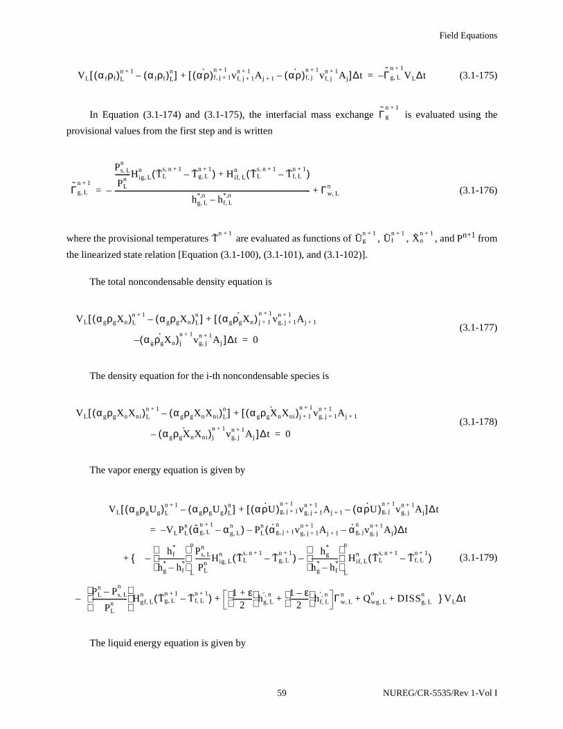
Field Equations
(3.1-175)
In Equation (3.1-174) and (3.1-175), the interfacial mass exchange is evaluated using the
provisional values from the first step and is written
(3.1-176)
where the provisional temperatures are evaluated as functions of , , , and Pn+1 from
the linearized state relation [Equation (3.1-100), (3.1-101), and (3.1-102)].
The total noncondensable density equation is
(3.1-177)
The density equation for the i-th noncondensable species is
(3.1-178)
The vapor energy equation is given by
(3.1-179)
The liquid energy equation is given by
VL α fρf( )Ln 1+ α fρf( )L
n–[ ] αρ·( )f j 1+,n 1+
vf j 1+,n 1+ Aj 1+ αρ·( )f j,
n 1+vf j,
n 1+ Aj–[ ]∆ t+ Γ g L,n 1+
VL∆t–=
Γ g
n 1+
Γ g L,n 1+
Ps L,n
PLn
---------Hig L,n TL
s n, 1+Tg L,
n 1+–( ) Hif L,
n TLs n 1+,
Tf L,n 1+
–( )+
hg L,*,n hf L,
*,n–--------------------------------------------------------------------------------------------------------------------– Γw L,
n+=
Tn 1+
Ugn 1+
Ufn 1+
Xnn 1+
VL αgρgXn( )Ln 1+ α gρgXn( )L
n–[ ] α gρgXn·( )[ j 1+
n 1+vg j 1+,
n 1+ Aj 1++
αgρgXn·( )j
n 1+vg j,
n 1+ Aj ]∆ t– 0=
VL αgρgXnXni( )Ln 1+ α gρgXnXni( )L
n–[ ] α gρgXn·
Xni( )j 1+n 1+
vg j 1+,n 1+ Aj 1+[+
αgρgXn·
Xni( )jn 1+
vg j,n 1+ Aj ]∆ t– 0=
VL α gρgUg( )Ln 1+ αgρgUg( )L
n–[ ] αρ U·( )g j 1+,
n 1+vg j 1+,
n 1+ Aj 1+ αρU·( )g j,
n 1+vg j,
n 1+ Aj–[ ]∆ t+
V– LPLn αg L,
n 1+ αg L,n–( ) PL
n α· g j 1+,n
vg j 1+,n 1+ Aj 1+ α· g j,
nvg j,
n 1+ Aj–( )∆t–=
{hf
*
hg* hf
*–----------------
L
nPs L,
n
PLn
---------Hig L,n TL
s n 1+,Tg L,
n 1+–( )–
hg*
hg* hf
*–----------------
L
n
Hif L,n TL
s n 1+,Tf L,
n 1+–( )–+
–PL
n P– s L,n
PLn
---------------------
Hgf L,n Tg L,
n 1+Tf L,
n 1+–( ) 1 ε+
2------------
hg L,′ n, 1 ε–
2-----------
hf L,′ n,+ Γw L,
n Q+ wg L,n
DISSg L,n } VL∆t+ +
59 NUREG/CR-5535/Rev 1-Vol I
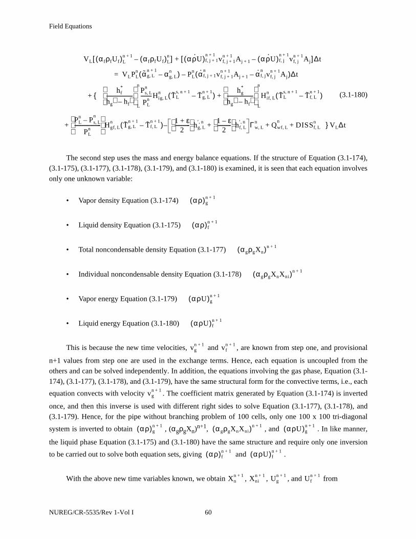
Field Equations
(3.1-180)
The second step uses the mass and energy balance equations. If the structure of Equation (3.1-174),
(3.1-175), (3.1-177), (3.1-178), (3.1-179), and (3.1-180) is examined, it is seen that each equation involves
only one unknown variable:
• Vapor density Equation (3.1-174)
• Liquid density Equation (3.1-175)
• Total noncondensable density Equation (3.1-177)
• Individual noncondensable density Equation (3.1-178)
• Vapor energy Equation (3.1-179)
• Liquid energy Equation (3.1-180)
This is because the new time velocities, and , are known from step one, and provisional
n+1 values from step one are used in the exchange terms. Hence, each equation is uncoupled from the
others and can be solved independently. In addition, the equations involving the gas phase, Equation (3.1-
174), (3.1-177), (3.1-178), and (3.1-179), have the same structural form for the convective terms, i.e., each
equation convects with velocity . The coefficient matrix generated by Equation (3.1-174) is inverted
once, and then this inverse is used with different right sides to solve Equation (3.1-177), (3.1-178), and
(3.1-179). Hence, for the pipe without branching problem of 100 cells, only one 100 x 100 tri-diagonal
system is inverted to obtain , (αgρgXn)n+1, , and . In like manner,
the liquid phase Equation (3.1-175) and (3.1-180) have the same structure and require only one inversion
to be carried out to solve both equation sets, giving and .
With the above new time variables known, we obtain , , , and from
VL α fρfUf( )Ln 1+ α fρfUf( )L
n–[ ] αρ U·( )f j 1+,
n 1+vf j 1+,
n 1+ Aj 1+ αρU·( )f j,
n 1+vf j,
n 1+ Aj–[ ]∆ t+
VLPLn αg L,
n 1+ αg L,n–( ) PL
n α· f j 1+,n
vf j 1+,n 1+ Aj 1+ α· f j,
nvf j,
n 1+ Aj–( )∆t–=
{+hf
*
hg∗ hf∗–---------------------
L
nPs L,
n
PLn
---------Hig L,n TL
s n 1+,Tg L,
n 1+–( )
hg*
hg∗ hf∗–---------------------
L
n
Hif L,n TL
s n 1+,Tf L,
n 1+–( )+
PLn P– s L,
n
PLn
---------------------
Hgf L,n Tg L,
n 1+Tf L,
n 1+–( ) 1 ε+
2------------
hg L,′ n, 1 ε–
2-----------
hf L,′ n,+– Γw L,
n Q+ wf L,n
DISSf L,n+ } VL∆t+
αρ( )gn 1+
αρ( )fn 1+
αgρgXn( )n 1+
αgρgXnXni( )n 1+
αρU( )gn 1+
αρU( )fn 1+
vgn 1+ vf
n 1+
vgn 1+
αρ( )gn 1+ α gρgXnXni( )n 1+ αρU( )g
n 1+
αρ( )fn 1+ αρU( )f
n 1+
Xnn 1+ Xni
n 1+ Ugn 1+ Uf
n 1+
NUREG/CR-5535/Rev 1-Vol I 60

Field Equations
(3.1-181)
(3.1-182)
(3.1-183)
(3.1-184)
The void fraction, , is obtained from
(3.1-185)
where
= the overall mixture density
= the liquid density, which is calculated from the linearized state relation
[Equation (3.1-97)] using Pn+1 and
= the vapor density, which is calculated from the linearized state relationship
[Equation (3.1-96)] using Pn+1, , and
Up to this point of this section on the nearly-implicit scheme, the difference equations have been
presented along with the time advancement for the case of two-phase to two-phase only. As indicated in
Section 3.1.4, there are three other possible transition cases (one-phase to one-phase, two-phase to one-
phase, and one-phase to two-phase). These three cases will now be described for the nearly-implicit
scheme.
For the one-phase to one-phase case, both the first step and the second step are carried out as in the
two-phase to two-phase case. For the phase that is not present, a large interfacial heat transfer coefficient
Xnn 1+ αgρgXn( )n 1+
αgρg( )n 1+-------------------------------=
Xnin 1+ αgρgXnXni( )n 1+
α gρgXn( )n 1+---------------------------------------=
Ugn 1+ αgρgUg( )n 1+
αgρg( )n 1+-------------------------------=
Ufn 1+ α fρfUf( )n 1+
α fρf( )n 1+-----------------------------=
αgn 1+
αgn 1+ ρm
n 1+ ρfn 1+
–
ρgn 1+ ρf
n 1+–
----------------------------αρ( )g
n 1+ αρ( )fn 1+ ρf
n 1+–+
ρgn 1+ ρf
n 1+–
----------------------------------------------------------------= =
ρmn 1+
ρfn 1+
Ufn 1+
ρgn 1+
Xnn 1+ Ug
n 1+
61 NUREG/CR-5535/Rev 1-Vol I

Field Equations
consistent with the interfacial heat transfer coefficients computed from the correlation for a void fraction of
10-5 is used. For the phase that is present, a value of 0.0 is used for the interfacial heat transfer coefficient.
For the phase that is not present, α is zero, and thus (αρ)n+1 equals zero for that phase. The provisional n+1
value of the corresponding variable is used in order to avoid the division by zero in Equation (3.1-181)
through (3.1-184). As with the semi-implicit time advancement, phasic energy, temperature, and density of
the missing phase are reset to the saturation values in the state relations subroutine.
For the two-phase to one-phase case (disappearance), the calculation is carried out the same as in the
two-phase to two-phase case. Then, for the phase that is missing, the phasic energy, temperature, and
density of the missing phase are reset to saturation values in the state relations subroutine as is done with
the one-phase to one-phase case. Sometimes when a phase disappears, the calculated void fraction and/or
noncondensable quality is less than zero or greater than one. When this occurs, the void fraction and/or
noncondensable quality is then reset to zero or one, respectively. If the calculated void fraction and/or
noncondensable quality is too much less than zero or too much greater than one (amount determined
through extensive testing, which is consistent with the mass error check), an error is assumed to have
occurred, and the time step is reduced and repeated. This is the same approach used in the semi-implicit
scheme time advancement.
For the one-phase to two-phase case (appearance), the first step quantities are used for the appearing
phase. A large interfacial heat transfer coefficient, consistent with the interfacial heat transfer coefficients
from the correlations, as if the void fraction were 10-5, is used for the appearing phase, resulting in the
energy and temperature of that phase being very close to saturation. Because the phase that is appearing is
assumed to appear at saturation conditions, an error can be made if, in reality, the phase appeared by
convection from a neighboring volume that was at a temperature different from saturation. The magnitude
of the potential error is controlled by letting the phase appear at saturation but restricting the amount that
can appear by time step control. If more than the limiting amount appears, an error is assumed to have
occurred, and the time step is reduced and repeated. This is the same approach used in the semi-implicit
scheme time advancement.
In summary, the second step stabilizes the convective terms in the mass and energy equations, and it
does so with very little computational effort due to the fractional step nature of the scheme. As an example,
if the nearly-implicit method is compared with the fully implicit method for a pipe without branching
problem of 100 cells, we have the following efficiency estimates. The fully implicit method requires the
inversion of a banded block tri-diagonal 600 x 600 matrix of bandwidth 23 containing 13,800 nonzero
elements. The nearly-implicit method requires the inversion of one block tri-diagonal 200 x 200 matrix
with 2 x 2 blocks and bandwidth 7 containing 1,400 nonzero elements plus two 100 x 100 tri-diagonal
matrices with 300 nonzero elements. The nearly-implicit method thus requires about 1/10 the number of
storage locations required by the fully implicit method. If the computational efficiency is estimated by
counting the number of multiplications in the forward part of a Gaussian elimination algorithm, then the
fully implicit method for this problem requires about 450,000 multiplications, whereas the nearly-implicit
method requires about 2,000 multiplications. Thus, the nearly-implicit method requires about 1/200 (based
NUREG/CR-5535/Rev 1-Vol I 62

Field Equations
on the number of multiplications) of the computational time per time step needed for a fully implicit
scheme.
3.1.6 Volume-Average Velocities
The previous development of the difference equations considered a pipe consisting of a series of
singly connected volumes without branching. In RELAP5/MOD3, each volume may have zero, one or
more junctions attached to its inlet end in the normal flow direction, and, zero, one, or more junctions
attached to its outlet end in the normal flow direction. The same can be true for the two crossflow
directions (see Section 3.4.5). Therefore, the flux terms at the inlet or outlet end of a volume for the normal
or crossflow directions consist of a summation over all of the junctions attached to that end of the volume.
Volume-average velocities are required for the momentum flux calculation, evaluation of the wall
frictional forces, evaluation of the wall heat transfer, evaluation of the interfacial heat transfer, and the
Courant time step limit. In a simple constant area passage, the arithmetic average between the inlet and
outlet is a satisfactory approximation. At branch volumes, however, with multiple inlets and/or outlets or
for volumes with abrupt area change, use of the arithmetic average results in nonphysical behavior.
The liquid and vapor velocities in the normal or crossflow directions in the volume cells are
calculated by a method that averages the phasic mass flows over the volume cell inlet and outlet junctions
in the normal or crossflow directions. A cell volume is shown in Figure 3.1-4, where the rectangular box
represents a cell volume. Each of the arrow vectors into or out of the box represents the liquid mass flow
through an inlet or outlet junction, respectively, in the normal or crossflow directions. The variable Jin is
the number of inlet junctions, and Jout is the number of outlet junctions. This discussion will be for liquid
velocity; the gas velocity derivation is the same.
At the inlet side of the volume, the total mass flow rate into the volume is given by
Figure 3.1-4 Schematic of a volume cell showing multiple inlet and outlet junction mass flows
Outlet
• •(αfρfvf)1A1
• •(αfρfvf)2A2
• •(αfρfvf)Jin-1AJin-1
• •(αfρfvf)JinAJin
• •(αfρfvf)JoutAJout
• •(αfρfvf)Jout-1AJout-1
• •(αfρfvf)2A2
• •(αfρfvf)1A1
•••
•••
Inlet
63 NUREG/CR-5535/Rev 1-Vol I
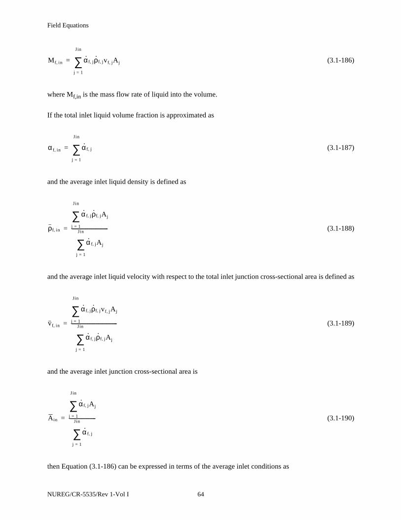
Field Equations
(3.1-186)
where Mf,in is the mass flow rate of liquid into the volume.
If the total inlet liquid volume fraction is approximated as
(3.1-187)
and the average inlet liquid density is defined as
(3.1-188)
and the average inlet liquid velocity with respect to the total inlet junction cross-sectional area is defined as
(3.1-189)
and the average inlet junction cross-sectional area is
(3.1-190)
then Equation (3.1-186) can be expressed in terms of the average inlet conditions as
Mf in, α· f j, ρ· f j, vf j, Aj
j 1=
Jin
∑=
α f in, α· f j,
j 1=
Jin
∑=
ρf in,
α· f j, ρ· f j, Aj
j 1=
Jin
∑
α· f j, Aj
j 1=
Jin
∑------------------------------=
vf in,
α· f j, ρ· f j, vf j, Aj
j 1=
Jin
∑
α· f j, ρ· f j, Aj
j 1=
Jin
∑--------------------------------------=
Ain
α· f j, Aj
j 1=
Jin
∑
α· f j,
j 1=
Jin
∑----------------------=
NUREG/CR-5535/Rev 1-Vol I 64
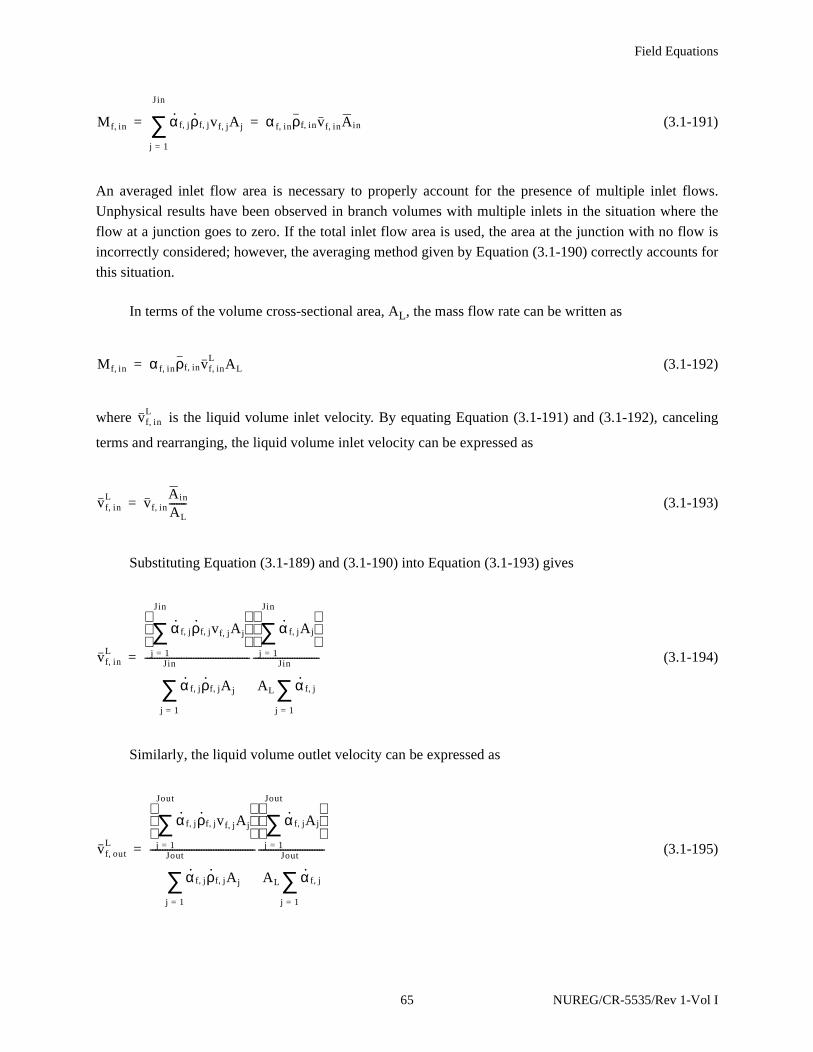
Field Equations
(3.1-191)
An averaged inlet flow area is necessary to properly account for the presence of multiple inlet flows.
Unphysical results have been observed in branch volumes with multiple inlets in the situation where the
flow at a junction goes to zero. If the total inlet flow area is used, the area at the junction with no flow is
incorrectly considered; however, the averaging method given by Equation (3.1-190) correctly accounts for
this situation.
In terms of the volume cross-sectional area, AL, the mass flow rate can be written as
(3.1-192)
where is the liquid volume inlet velocity. By equating Equation (3.1-191) and (3.1-192), canceling
terms and rearranging, the liquid volume inlet velocity can be expressed as
(3.1-193)
Substituting Equation (3.1-189) and (3.1-190) into Equation (3.1-193) gives
(3.1-194)
Similarly, the liquid volume outlet velocity can be expressed as
(3.1-195)
Mf in, α· f j, ρ· f j, vf j, Aj
j 1=
Jin
∑ α f in, ρf in, vf in, Ain= =
Mf in, α f in, ρf in, vf in,L AL=
vf in,L
vf in,L vf in,
Ain
AL-------=
vf in,L
α· f j, ρ· f j, vf j, Aj
j 1=
Jin
∑
α· f j, ρ· f j, Aj
j 1=
Jin
∑-------------------------------------------
α· f j, Aj
j 1=
Jin
∑
AL α· f j,
j 1=
Jin
∑---------------------------=
vf out,L
α· f j, ρ· f j, vf j, Aj
j 1=
Jout
∑
α· f j, ρ· f j, Aj
j 1=
Jout
∑-------------------------------------------
α· f j, Aj
j 1=
Jout
∑
AL α· f j,
j 1=
Jout
∑---------------------------=
65 NUREG/CR-5535/Rev 1-Vol I

Field Equations
In RELAP5/MOD1, the total liquid momentum of the volume was expressed in terms of the
momentum of the inlet and outlet halves of the volume as (assuming density changes are small)
(3.1-196)
Thus,
(3.1-197)
Substitution of Equation (3.1-194) and (3.1-195) into Equation (3.1-197) yields
(3.1-198)
for liquid and
(3.1-199)
for vapor, where old time levels (n) are used for time varying quantities.
Equation (3.1-198) and (3.1-199) are used for the momentum flux calculation, evaluation of the
interfacial heat transfer, and the Courant time step limit. For the evaluation of the wall frictional forces,
different formulas are used.
For the evaluation of the wall frictional forces, the magnitude of the volume velocities is needed. An
obvious way to compute this magnitude is to take just the absolute value of the result from Equation (3.1-
198) and (3.1-199). A problem can occur when the magnitude is zero because the inlet velocity is equal
and opposite to the outlet velocity. To avoid this case, the calculation of the magnitude of the volume
velocities used in the wall friction uses the same form as Equation (3.1-200) and (3.1-201), with the
ρf L, VLvf L,12---ρf L, VLvf in,
L 12---ρf L, VLvf out,
L+=
vf L,12--- vf in,
L vf out,L+( )=
vf L,n 1
2---
α· f j,n
j 1=
Jin
∑ ρ· f j,n
vf j,n Aj
α· f j,n
Aj
j 1=
Jin
∑
AL α· f j,n ρ· f j,
nAj
j 1=
Jin
∑
α· f j,n
j 1=
Jin
∑
------------------------------------------------------------------------12---
α· f j,n
j 1=
Jout
∑ ρ· f j,n
vf j,n Aj
α· f j,n
Aj
j 1=
Jout
∑
AL α· f j,n ρ· f j,
nAj
j 1=
Jout
∑
α· f j,n
j 1=
Jout
∑
------------------------------------------------------------------------+=
NUREG/CR-5535/Rev 1-Vol I 66
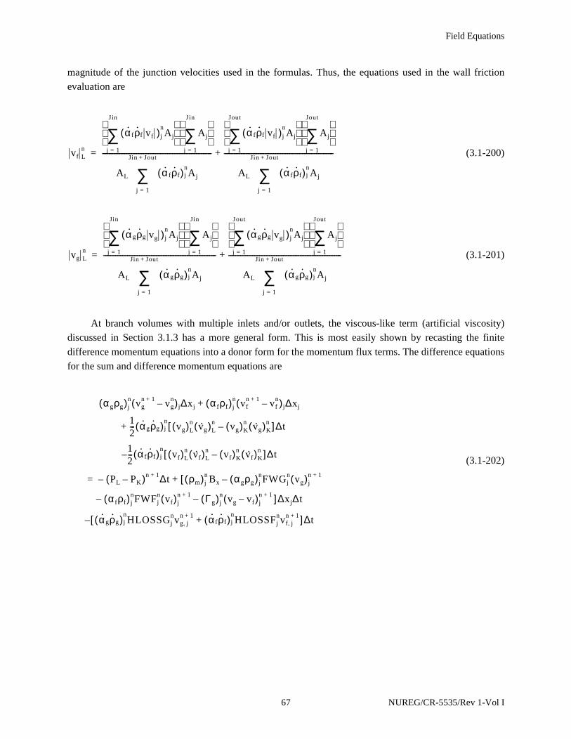
Field Equations
magnitude of the junction velocities used in the formulas. Thus, the equations used in the wall friction
evaluation are
(3.1-200)
(3.1-201)
At branch volumes with multiple inlets and/or outlets, the viscous-like term (artificial viscosity)
discussed in Section 3.1.3 has a more general form. This is most easily shown by recasting the finite
difference momentum equations into a donor form for the momentum flux terms. The difference equations
for the sum and difference momentum equations are
(3.1-202)
vf Ln
α· fρ· f vf( )jnAj
j 1=
Jin
∑
Aj
j 1=
Jin
∑
AL α· fρ· f( )jnAj
j 1=
Jin Jout+
∑----------------------------------------------------------------
α· fρ· f vf( )jnAj
j 1=
Jout
∑
Aj
j 1=
Jout
∑
AL α· fρ· f( )jnAj
j 1=
Jin Jout+
∑----------------------------------------------------------------+=
vg Ln
α· gρ· g vg( )jnAj
j 1=
Jin
∑
Aj
j 1=
Jin
∑
AL α· gρ· g( )jnAj
j 1=
Jin Jout+
∑------------------------------------------------------------------
α· gρ· g vg( )jnAj
j 1=
Jout
∑
Aj
j 1=
Jout
∑
AL α· gρ· g( )jnAj
j 1=
Jin Jout+
∑------------------------------------------------------------------+=
αgρg( )jn vg
n 1+ vgn–( )j∆xj α fρf( )j
n vfn 1+ vf
n–( )j∆xj+
12--- α· gρ· g( )j
nvg( )L
n v· g( )Ln vg( )K
n v· g( )Kn–[ ]∆ t+
12--- α· fρ· f( )j
nvf( )L
n v· f( )Ln vf( )K
n v· f( )Kn–[ ]∆ t–
PL PK–( )n 1+ ∆t– ρm( )jn[ Bx αgρg( )j
nFWGjn vg( )j
n 1+–+=
α fρf( )jnFWFj
n vf( )jn 1+– Γ g( )j
n vg vf–( )jn 1+ ]∆xj∆t–
α· gρ· g( )jnHLOSSGj
nvg j,n 1+ α· fρ· f( )j
nHLOSSFj
nvf j,n 1++[ ]∆ t–
67 NUREG/CR-5535/Rev 1-Vol I

Field Equations
(3.1-203)
where the donored volume liquid velocity for the L volume is from
(3.1-204)
Here, is from Equation (3.1-194), is from Equation (3.1-195), and is from Equation (3.1-
198). Similarly, the donored volume gas velocity for the L volume is from
(3.1-205)
The donored volume liquid and gas velocities for the K volume are similar. The momentum flux
terms that use the velocities shown here default to the equation shown in Section 3.1.3 for a pipe with no
branching.
1Cρm
2
ρgρf----------+
j
n
vgn 1+ vg
n–( ) vfn 1+ vf
n–( )–[ ] j∆xj
12---
α· gρ· g
αgρg-----------
j
n
vg( )Ln v· g( )L
n vg( )Kn v· g( )K
n–[ ]∆ t+
12---
α· fρ· f
α fρf----------
j
n
vf( )Ln v· f( )L
n vf( )Kn v· f( )K
n–[ ]∆ t–
ρf ρ– g
ρgρf-------------
j
n
PL PK–( )n 1+ ∆t–=
FWGjn vg( )j
n 1+ FWFjn vf( )j
n 1+–{–
Γ gn ρm
n vIn 1+ α f
nρfnvg
n 1+– αgnρg
nvfn 1+–( )
αgρgα fρf( )n---------------------------------------------------------------------------------------
j
–
ρmFI( )jn vg
n 1+( vfn 1+ )j– }∆ xj∆t
α· gρ· g
αgρg-----------
j
n
HLOSSGjnvg j,
n 1+–+
α· fρ· f
α fρf----------
j
n
HLOSSFjnvf j,
n 1+ ]∆ t–
ρm
ρgρf----------
j
n
ρf ρg–( )jnBy yL yK–( )∆t+
v· f( )Ln 1
2--- vf in,
L vf out,L+( ) 1
2---
vf( )Ln
vf( )Ln
-------------- vf in,L vf out,
L–( )+=
vf in,L vf out,
L vf( )Ln
v· g( )Ln 1
2--- vg in,
L vg out,L+( ) 1
2---
vg( )Ln
vg( )Ln
--------------- vg in,L vg out,
L–( )+=
NUREG/CR-5535/Rev 1-Vol I 68
Field Equations
3.1.7 Implicit Hydrodynamic and Heat Structure Coupling
An option exists to implicitly couple the time advancement of the hydrodynamic and heat structure
models. Heat structures represent the solid structures bounding hydrodynamic volumes (i.e., pipe walls) or
structures internal to the volumes (fuel pins). One-dimensional heat conduction is used to compute
temperature distributions within heat structures. Hydrodynamic and heat structure conditions are coupled
through heat structure boundary conditions. The solution matrix for the set of simultaneous equations
resulting from the implicit coupling of hydrodynamic and heat structure advancement contains the same
number of nonzero elements as discussed in the previous sections but with some of the elements having
additional terms. In addition, the total set of simultaneous equations includes an equation from each mesh
point of each heat structure attached to the hydrodynamic volumes. The heat conduction equations have
additional terms related to fluid temperatures introduced in the boundary conditions. This larger set of
simultaneous equations, however, is solved with only a modest increase in computations compared to the
explicit coupling. This implicit coupling can be used with either the semi-implicit or nearly-implicit
advancement.
The purpose of the implicit coupling of hydrodynamic and heat structure time advancement is to
more accurately model the exchange of energy between the structures and fluid in the volumes, to avoid
numerical instabilities due to explicit coupling, and to achieve reduction of computing time through larger
time steps.
The purpose of the remainder of this section is to show the additional terms added to the
hydrodynamic equations because of the implicit coupling. A complete understanding of the implicit
coupling requires information from Section 4 describing numerical techniques for heat structures,
information from Section 3.3.10 describing heat transfer correlations, and information from Volume IV,
describing relationships between heat transfer from structures, heat added to volumes, and mass transfer
associated with wall heat transfer. Equation (3.1-209) through (3.1-212) follow directly from the material
in Volume IV.
In previous subsections [see Equation (3.1-5) and (3.1-13)], the quantities, Γw, Qwg, and Qwf, which
are related to heat and mass transfer at and near the wall surface, were introduced. These were discussed as
if only one wall surface could be attached to a volume. Similarly to the possibility of multiple junctions
being connected to the ends of a volume, multiple wall surfaces representing quite different heat transfer
situations can be attached to a volume. Thus the Γw, Qwg, and Qwf quantities involve summations over the
surfaces attached to a volume. Details of the summations are shown in Volume IV.
The previous section combined boiling and condensation in the Γw quantity, but showed a difference
in the two situations through the factor ε [Equation (3.1-31) and (3.1-32)]. That notation is correct for one
heat structure connected to a volume and relies on the wall surface possibly boiling, or condensing, but not
both simultaneously. With multiple heat structures, some might be boiling and others could be condensing.
Accordingly, boiling mass transfer, Γw, and condensing mass transfer, Γc, are separated. Thus, the total
69 NUREG/CR-5535/Rev 1-Vol I

Field Equations
mass transfer consists of mass transfer in the bulk fluid (Γig) and mass transfer in the boundary layers near
the walls (Γw and Γc), that is,
(3.1−206)
With implicit hydrodynamic and heat structure coupling, some source terms in the mass and energy
equations for the semi-implicit and nearly-implicit scheme become implicit. In the continuity equations,
Γw becomes . In the vapor energy equations, terms involving Γw and Qwg becomes
(3.1-207)
In the liquid energy equations, terms involving Γw and Qwf becomes
(3.1-208)
Volume IV discusses multiple heat structures connected to hydrodynamic volumes. Summations
over the multiple heat structures that can be connected to hydrodynamic volumes are discussed. After
applying the summations discussed in Volume IV, the wall heat transfer and mass transfer terms can be
written as
(3.1-209)
(3.1-210)
(3.1-211)
(3.1-212)
Γ g Γ ig Γw Γ c+ +=
Γw L,n 1+
Γ c L,n 1+
+
Γw L,n 1+
hg L,s n, Γ c L,
n 1+hf L,
s n, Qwg L,n 1+
+ +
Γw L,n 1+
hg L,s n, Γ c L,
n 1+hf L,
s n,– Qwf L,n 1+
+–
Qwfn 1+
Qwf0n Qwff
n Tfn 1+
Tfn–( ) Qwfg
n Tgn 1+
Tgn–( ) Qwft
n Tts n 1+,
Tts n,–( )+ + +=
Qwfpn T
s n 1+,Ts n,–( )+
Qwgn 1+
Qwg0n Qwgf
n Tfn 1+
Tfn–( ) Qwgg
n Tgn 1+
Tgn–( ) Qwgt
n Tts n 1+,
Tts n,–( )+ + +=
Qwgpn T
s n 1+,Ts n,–( )+
Γw
n 1+Γwf
n 1+Γwf0
n Γwffn Tf
n 1+Tf
n–( ) Γwfgn Tg
n 1+Tg
n–( ) Γwftn Tt
s n 1+,Tt
s n,–( )+ + += =
Γwfpn T
s n 1+,Ts n,–( )+
Γ c
n 1+Γwg
n 1+Γwg0
n Γwgfn Tf
n 1+Tf
n–( ) Γwggn Tg
n 1+Tg
n–( ) Γwgtn Tt
s n 1+,Tt
s n,–( )+ + += =
Γwgpn T
s n 1+,Ts n,–( )+
NUREG/CR-5535/Rev 1-Vol I 70
Field Equations
The variables are given by Equation (3.1-100) through (3.1-102), where Ts
is the saturation temperature. When noncondensables are present, this Ts is based on the partial pressure of
steam [Ts(Ps)]. Some of the heat transfer terms, when noncondensables are present, use the saturation
temperature based on the total pressure P = Ps + Pn. In Equation (3.1-209) through (3.1-212), the saturation
temperature based on Ps is denoted by Ts(Ps) and the saturation temperature based on P is denoted by
. Thus, is given by
(3.1-213)
When the implicit coupling of the hydrodynamics and the heat slabs is used, additional terms are
added to some of the terms of the matrix in Equation (3.1-115). These additional terms are next shown
as additions to the matrix elements listed in Equation (3.1-118) through (3.1-141).
(3.1-214)
(3.1-215)
(3.1-216)
(3.1-217)
(3.1-218)
(3.1-219)
Ts n 1+,
Tgn 1+
and Tfn 1+
, ,
Tts P( ) Tt L,
s n 1+,P( )
Tt L,s n 1+,
P( ) Tt L,s n, P( )
dTts
dP--------
L
n
PLn 1+ PL
n–( )+=
A˜
A˜
A21 A21 ∆t Qwgg Γwfghgs Γwgghf
s+ +( )∂Tg
∂Xn---------– ∆t Qwgp Γwfphg
s Γwgphfs+ +( ) ∂Ts
∂Xn---------–=
A22 A22 ∆t Qwgg Γwfghgs Γwgghf
s+ +( )∂Tg
∂Ug---------– ∆t Qwgp Γwfphg
s Γwgphfs+ +( ) ∂Ts
∂Ug---------–=
A23 A23 ∆t Qwgf Γwffhgs Γwgfhf
s+ +( )∂Tf
∂Uf---------–=
A25 A25 ∆t Qwgf Γwffhgs Γwgfhf
s+ +( )∂Tf
∂P--------– ∆t Qwgg Γwfghg
s Γwgghfs+ +( )
∂Tg
∂P---------–=
∆t Qwgp Γwfphgs Γwgphf
s+ +( )∂Ts
∂P-------- ∆t Qwgt Γwfthg
s Γwgthfs+ +( )
dTts
dP--------––
A31 A31 ∆t Qwfg Γwfg– hgs Γwgg– hf
s( )∂Tg
∂Xn---------– ∆t Qwfp Γwfp– hg
s Γwgp– hfs( ) ∂Ts
∂Xn---------–=
A32 A32 ∆t Qwfg Γwfg– hgs Γwgg– hf
s( )∂Tg
∂Ug---------– ∆t Qwfp Γwfp– hg
s Γwgp– hfs( ) ∂Ts
∂Ug---------–=
71 NUREG/CR-5535/Rev 1-Vol I

Field Equations
(3.1-220)
(3.1-221)
(3.1-222)
(3.1-223)
(3.1-224)
(3.1-225)
3.1.8 Numerical Solution of Boron Transport Equation
The boron field and its attendant modeling assumptions were discussed in Section 3.1.1.3. The
default numerical scheme for boron solute tracking is the upwind difference scheme; a second-order
accurate Godunov scheme can also be used and is activated by the user in the input deck. These two
schemes will next be discussed.
3.1.8.1 Upward Difference Scheme.
Applying the upwind difference scheme to the boron differential Equation (3.1-51) for the semi-
implicit scheme, gives
(3.1-226)
Here, the boron densities in the convective terms are evaluated at old time.
A33 A33 ∆t Qwff Γwff– hgs Γwgf– hf
s( )∂Tf
∂Uf---------–=
A35 A35 ∆t Qwff Γwff– hgs Γwgf– hf
s( )∂Tf
∂P--------– ∆t Qwfg Γwfg– hg
s Γwgghfs+( )
∂Tg
∂P---------–=
∆t Qwfp Γwfp– hgs Γwgp– hf
s( )∂Ts
∂P-------- ∆t Qwft Γwft– hg
s Γwgt– hfs( )
dTts
dP--------––
A41 A41 2∆t Γwfg Γwgg+( )∂Tg
∂Xn---------– 2∆t Γwfp Γwgp+( ) ∂Ts
∂Xn---------–=
A42 A42 2∆t Γwfg Γwgg+( )∂Tg
∂Ug---------– 2∆t Γwfp Γwgp+( ) ∂Ts
∂Ug---------–=
A43 A43 2∆t Γwff Γwgf+( )∂Tf
∂Uf---------–=
A45 A45 2∆t Γwff Γwgf+( )∂Tf
∂P--------– 2∆t Γwfg Γwgg+( )
∂Tg
∂P---------–=
2∆t Γwfp Γwgp+( )∂Ts
∂P-------- 2∆t Γwft Γwgt+( )
dTts
dP--------––
VL ρb L,n 1+ ρb L,
n–( ) ρ· b j 1+,n
vf j 1+,n 1+ Aj 1+ ρ· b j,
nvf j,
n 1+ Aj–( )∆t+ 0=
NUREG/CR-5535/Rev 1-Vol I 72
Field Equations
Applying the upwind scheme to the boron differential Equation (3.1-51) for the nearly-implicit
scheme gives
(3.1-227)
Here, the boron densities in the convective terms are evaluated at new time. The coefficient matrix
generated by the liquid continuity Equation (3.1-175) is used.
3.1.8.2 Godunov Scheme.
Accurate calculation of the boron field is required to simulate the coupled hydrodynamics and
neutron behavior of a reactor. Recent advances in shock-capturing schemes or the TVD schemes (the
oscillation-suppression strategy of the total-variation diminishing scheme) achieve impressive results for
the numerical solution of the defective transport equations.3.1-19,3.1-20,3.1-21 These schemes use locally
varying positive artificial diffusion or viscosity (first order upwind) to suppress oscillations combined with
local negative viscosity (such as first order downwind) to compress or steepen the front. Rider and
Woodruff3.1-22 reported that an algorithm using a second-order accurate Godunov method with a highly
compressive limiter can adequately solve the defective transport equation for solute tracking. This method
is chosen to solve the boron transport Equation (3.1-51) because it is consistent with RELAP5 numerics
and is applicable to complex geometry.
A second-order accurate Godunov method to solve the boron transport equation was implemented in
RELAP5/MOD3. The new method significantly improves the results as compared with that using the
highly diffusive first-order upwind difference previously used.
The equation governing boron transport, Equation (3.1-51), can be rewritten in a control volume (V)
with surface area as:
(3.1-228)
The use of the second-order accurate Godunov method to solve Equation (3.1-228) is well
documented by Rider and Woodruff. The essential numerics are summarized below.
The numerical solution of Equation (3.1-228) can be written as
(3.1-229)
VL ρb L,n 1+ ρb L,
n–( ) ρ· b j 1+,n 1+
vf j 1+,n 1+ Aj 1+ ρ· b j,
n 1+vf j,
n 1+ Aj–( )∆t+ 0=
A˜
∂ρb
∂t--------dV ρbv
˜f dA
˜•
A˜
∫+v
∫ 0=
ρb L,n 1+ ρb L,
n ∆tVL------AjFj
n ∆tVL------Aj 1+ Fj 1+
n–+=
73 NUREG/CR-5535/Rev 1-Vol I
Field Equations
The flux is expressed by
(3.1-230)
where
(3.1-231)
(3.1-232)
(3.1-233)
A similar equation can be written for .
The cell-centered limited gradient is given as
(3.1-234)
Note that both the superbee limiter of Roe3.1-23 and artificial compression3.1-24 (1 + θL ωL)
are introduced. This step is necessary because the number of grid points in modeling the reactor system
tend to be relatively small. It also ensures that the method is a TVD scheme.3.1-21 The superbee limiter is
defined as
(3.1-235)
where
(3.1-236)
Fj 1+n
Fj 1+n 1
2--- vfj 1+
n12---+
ρb j 1+,n L, ρb j 1+,
n R,+( ) vfj 1+
n12---+
ρb j 1+,n L, ρb j 1+,
n R,–( )+=
vfj 1+
n12---+
v12--- vfj 1+
n 1+ vfj 1+
n+( )= =
ρb j 1+,n L, ρb L,
n 12---∆xL
1v∆t∆xL---------–
SL+=
ρb j 1+,n R, ρb M,
n 12---∆xM
1v∆t∆xM----------+
SM–=
Fjn
SL
SL 1 θLωL+( )Φ r 1,( )Sj 1+ 1 θLωL+( )Φ r 1,( )ρb M,
n ρb L,n–
∆xj 1+--------------------------
= =
Φ r 1,( )
Φ r 1,( ) max 0 min 2r 1,( ) min r 2,( ),,[ ]=
rSj
Sj 1+----------=
NUREG/CR-5535/Rev 1-Vol I 74

Field Equations
(3.1-237)
(3.1-238)
In the artificial compression (1 + θL ωL), the discontinuity detector θL is given as
(3.1-239)
The parameter ωL is chosen to be a function of the local Courant number
(3.1−240)
In modeling a reactor system, there are components containing volumes to which multiple junctions
are connected to form a multi-dimensional flow network. The cell-centered limited gradient is set to
zero in these volumes and the Godunov scheme reverts to the upwind difference scheme for these volumes.
The above numerical solution is used when the semi-implicit scheme is chosen to solve the field
equations. If the nearly-implicit scheme is employed to solve the field equations, the time-step used in the
scheme may be greater than the material Courant limit. A subcycling calculation of the boron transport is
implemented for the nearly-implicit scheme. In the method, the boron transport is integrated within each
large time step taken by the advancement of the field equations. The time step used in the boron calculation
is limited by the Courant condition. The fluid velocity used in the boron calculation is interpolated from
the results of the field equations. The boron transport is calculated in such a fashion such that solutions of
the field equations and boron transport are synchronized in the same large time step.
3.1.9 References
3.1-1. V. H. Ransom. Course A--Numerical Modeling of Two-Phase Flows for Presentation at Ecoled’Ete d’Analyse Numerique. EGG-EAST-8546. Idaho National Engineering Laboratory. May1989.
3.1-2. M. Ishii. Thermo-Fluid Dynamic Theory of Two-Phase Flow. Collection de la Direction desEtudes d’Recherches of Electricute de France. 1975.
3.1-3. F. H. Harlow and A. A. Amsden. “Flow of Interpenetrating Material Phases.” Journal ofComputational Physics. 18. 1975. pp. 440-464.
Sj
ρb L,n ρb K,
n–∆xj
-------------------------=
Sj 1+
ρb M,n ρb L,
n–∆xj 1+
--------------------------=
θL1 r–
1 r+--------------=
νL
vL∆t∆xL-----------=
ωL min vL 1 vL–,( )=
SL
75 NUREG/CR-5535/Rev 1-Vol I

Field Equations
3.1-4. P. S. Anderson, P. Astrup, L. Eget, and O. Rathman. “Numerical Experience with the Two-FluidModel RISQUE.” Proceedings from Topical Meeting on Thermal Reactor Safety, Sun Valley, ID.July 31-August 4, 1977.
3.1-5. N. Zuber. “On the Dispersed Two-Phase Flow in the Laminar Flow Regime.” ChemicalEngineering Science. 19. 1964. pp. 897-917.
3.1-6. L. Van Wijngaarden. “Hydrodynamic Interaction between Gas and Bubbles in Liquid.” Journalof Fluid Mechanics. 77. 1. 1976. pp. 27-44.
3.1-7. R. T. Lahey, Jr. “RPI Two-Phase Flow Modeling Program.” Fifth Water Reactor Safety ResearchInformation Meeting, Washington, D.C. November 7-11, 1977.
3.1-8. D. A. Drew, L. Y. Cheng, and R. T. Lahey, Jr. “The Analysis of Virtual Mass Effects in Two-Phase Flow.” International Journal of Multiphase Flow. 5. 1979. pp. 233-242.
3.1-9. J. A. Trapp and V. H. Ransom. “A Choked-Flow Calculation Criterion for Nonhomogeneous,Nonequilibrium Two-Phase Flows.” International Journal of Multiphase Flow. 8. 6. 1982.pp. 669-681.
3.1-10. A. R. Curtis and J. K. Reid. FORTRAN Subroutines for the Solution of Sparse Sets of LinearEquations. AERE-R6844. Atomic Energy Research Establishment Harwell. 1971.
3.1-11. D. Gidaspow (Chairman). “Modeling of Two-Phase Flow.” Proceedings of Round TableDiscussion RT-1-2 at the Fifth International Heat Transfer Conference, Tokyo, Japan. September3-7, 1974. also in ASME Journal of Heat Transfer. 3. 1974.
3.1-12. J. D. Ramshaw and J. A. Trapp. “Characteristics, Stability, and Short-Wavelength Phenomena inTwo-Phase Flow Equation Systems.” Nuclear Science and Engineering. 66. 1978. pp. 93-102.
3.1-13. J. J. Dongarra, C. B. Moler, J. R. Bunch, and G. W. Stewart. LINPACK User’s Guide. SIAM:Philadelphia, PA. 1979.
3.1-14. H. B. Stewart. “Fractional Step Methods for Thermohydraulic Calculations.” Journal ofComputational Physics. 40. 1981. pp. 77-90.
3.1-15. J. H. Mahaffy. “A Stability-Enhancing Two-Step Method for Fluid Flow Calculations.” Journalof Computational Physics. 46. 1982. pp. 329-341.
3.1-16. J. A. Trapp and R. A. Riemke. “A Nearly-Implicit Hydrodynamic Numerical Scheme for Two-Phase Flows.” Journal of Computational Physics. 66. 1986. pp. 62-68.
3.1-17. A. S. Shieh and R. A. Riemke. “Diagonally Dominant Enhancement Methods for Matrix Solversin RELAP5.” Nuclear Science and Engineering. 105. 1990. pp. 404-408.
NUREG/CR-5535/Rev 1-Vol I 76
Field Equations
3.1-18. V. H. Ransom et al. RELAP5/MOD1 Code Manual. NUREG/CR-1826, EGG-2070. IdahoNational Engineering Laboratory. March 1982.
3.1-19. H. C. Yee. Upwind and Symmetric Shock-Capturing Schemes. NASA Technical Memorandum1000916. Ames Research Center. 1987.
3.1-20. B. P. Leonard. Universal Limiter for Transient Interpolation Modeling of the AdvectiveTransport Equation: The ULTIMATE Conservative Difference Scheme. NASA TechnicalMemorandum 1000916. Ames Research Center. 1988.
3.1-21. W. J. Rider. Design of High Resolution Upwind Shock-Capturing Methods. LA-12327-T. LosAlamos National Laboratory. 1992.
3.1-22. W. J. Rider and S. B. Woodruff. High-Order Solute Tracking in Two-Phase Thermal Hydraulics.LA-UR-91-2263. Los Alamos National Laboratory. 1991.
3.1-23. P. L. Roe. “Some Contributions to the Modeling of Discontinuous Flow.” Lectures in AppliedMathematics. 22. Part 2. 1975. pp. 163-193.
3.1-24. H. C. Yee and R. F. Warming. “Implicit Total Variation Diminishing (TVD) Schemes for Steady-State Calculations.” Journal of Computational Physics. 57. 1985. pp. 327-360.
77 NUREG/CR-5535/Rev 1-Vol I

Field Equations
NUREG/CR-5535/Rev 1-Vol I 78

State Relationships
3.2 State Relationships
The six-equation model uses five independent state variables with an additional equation for the
noncondensable gas component. The independent state variables are chosen to be P, αg, Ug, Uf, and Xn.
All the remaining thermodynamic variables (temperatures, densities, partial pressures, qualities, etc.) are
expressed as functions of these five independent state variables. In addition to these variables, several state
derivatives are needed for some of the linearizations used in the numerical scheme. This section contains
three parts. The first discusses the state property derivatives needed in the numerical scheme. The second
section develops the appropriate derivative formulas for the single component case. The third section does
the same for the two-phase, two-component case.
3.2.1 State Equations
To expand the time derivatives of the phasic densities in terms of these independent state variables
using two-term Taylor series expansions, the following derivatives of the phasic densities are needed:
The interphase mass and heat transfer models use an implicit (linearized) evaluation of the
temperature potentials and . The quantity is the temperature that exists at the phase
interface. For a single-component mixture, we have
(3.2-1)
where the superscript s denotes a saturation value. In the presence of a noncondensable mixed with the
steam, we assume3.2-1
(3.2-2)
where is the partial pressure of the steam in the gaseous phase. The gaseous phase properties for a two-
component mixture can be described with three independent properties.3.2-2 In particular, the steam partial
pressure, , can be expressed as
(3.2-3)
∂ρg
∂P--------
Ug Xn,
, ∂ρg
∂Ug---------
P Xn,
, ∂ρg
∂Xn---------
P Ug,
, ∂ρf
∂P--------
Uf
, ∂ρf
∂Uf---------
P
Tf TI– Tg TI– TI
TI Ts P( )=
TI Ts Ps( )=
Ps
Ps
Ps Ps P Xn Ug, ,( )=
79 NUREG/CR-5535/Rev 1-Vol I

State Relationships
Substituting Equation (3.2-3) into (3.2-2) gives the interface temperature, TI, as the desired function
of P, , and .a The implicit (linearized) evaluation of the temperature potentials in the numerical
scheme requires the following derivatives of the phasic and interface temperatures:
If we have a single component, the derivatives are zero and
(3.2-4)
since is only a function of P for this case.
In addition to these derivatives, the basic phasic properties as functions of P, , , and are
needed, along with the homogeneous equilibrium sound speed for the critical flow model.
The basic properties are calculated from thermodynamic tables3.2-3 that tabulate saturation properties
as a function of temperature, saturation properties as a function of pressure, and single-phase properties as
a function of pressure and temperature. The properties and derivatives in the tables are saturation pressure,
saturation temperature, specific volume (υ), specific internal energy, and three derivatives [the isobaric
thermal expansion coefficient (β), the isothermal compressibility (κ), and the specific heat at constant
pressure ( )].
3.2.2 Single-Component, Two-Phase Mixture
For the purposes of this manual, a single-component, two-phase mixture is referred to as Case 1.
Case 1 is straightforward. Liquid properties are obtained from the steam tables, given P and . All the
desired density and temperature derivatives can then be obtained from the derivatives , , and .3.2-4
The desired derivatives are given as
(3.2-5)
a. The properties and could have initially been written with , , as the independent arguments.
Equation (3.2-3) would then be used to write and , with P, , and as the independent variables.
Xn Ug
ρg Tg Ps Xn Ug
ρg Tg Xn Ug
∂Tg
∂P---------
Ug Xn,
, ∂Tg
∂Ug---------
P Xn,
, ∂Tg
∂Xn---------
P Ug,
, ∂Tf
∂P--------
Uf
, ∂Tf
∂Uf---------
P
∂Ts
∂P--------
Ug Xn,
, ∂Ts
∂Ug---------
P Xn,
, ∂Ts
∂Xn---------
P Ug,
,
Xn
∂Ts
∂Ug---------
P
0=
Ts
Ug Uf Xn
Cp
Uf
κ f βf Cpf
∂ρf
∂Uf---------
P
υ fβf
Cpf υ fβfP–( )υ f2
--------------------------------------–=
NUREG/CR-5535/Rev 1-Vol I 80
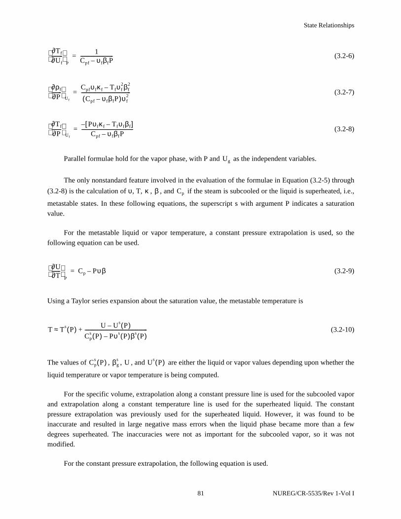
State Relationships
(3.2-6)
(3.2-7)
(3.2-8)
Parallel formulae hold for the vapor phase, with P and as the independent variables.
The only nonstandard feature involved in the evaluation of the formulae in Equation (3.2-5) through
(3.2-8) is the calculation of υ, T, , , and if the steam is subcooled or the liquid is superheated, i.e.,
metastable states. In these following equations, the superscript s with argument P indicates a saturation
value.
For the metastable liquid or vapor temperature, a constant pressure extrapolation is used, so the
following equation can be used.
(3.2-9)
Using a Taylor series expansion about the saturation value, the metastable temperature is
(3.2-10)
The values of , , , and are either the liquid or vapor values depending upon whether the
liquid temperature or vapor temperature is being computed.
For the specific volume, extrapolation along a constant pressure line is used for the subcooled vapor
and extrapolation along a constant temperature line is used for the superheated liquid. The constant
pressure extrapolation was previously used for the superheated liquid. However, it was found to be
inaccurate and resulted in large negative mass errors when the liquid phase became more than a few
degrees superheated. The inaccuracies were not as important for the subcooled vapor, so it was not
modified.
For the constant pressure extrapolation, the following equation is used.
∂Tf
∂Uf---------
P
1Cpf υ fβfP–---------------------------=
∂ρf
∂P--------
Uf
Cpfυ fκ f Tfυ f2βf
2–
Cpf υ fβfP–( )υ f2
-----------------------------------------=
∂Tf
∂P--------
Uf
Pυ fκ f Tfυ fβf–[ ]–Cpf υ fβfP–
-------------------------------------------=
Ug
κ β Cp
∂U∂T-------
P
Cp Pυβ–=
T Ts P( ) U Us P( )–
Cps P( ) Pυs P( )βs P( )–
----------------------------------------------------+≈
Cps P( ) βg
s U Us P( )
81 NUREG/CR-5535/Rev 1-Vol I
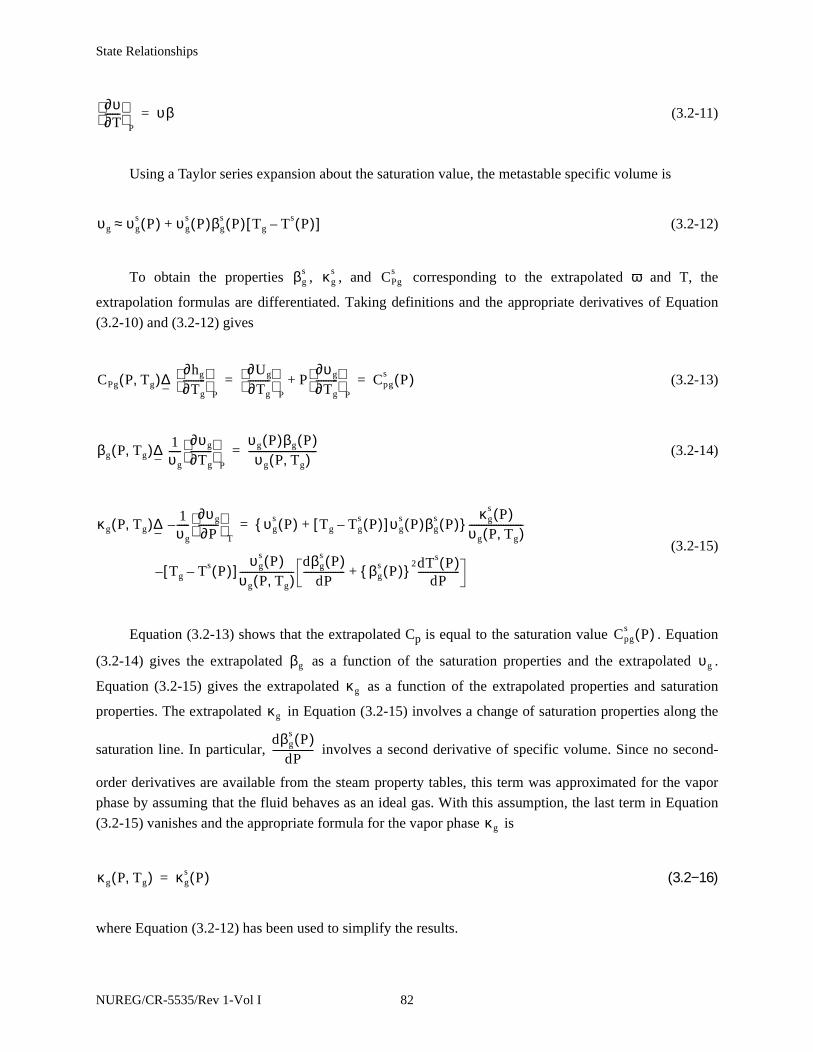
State Relationships
(3.2-11)
Using a Taylor series expansion about the saturation value, the metastable specific volume is
(3.2-12)
To obtain the properties , , and corresponding to the extrapolated ϖ and T, the
extrapolation formulas are differentiated. Taking definitions and the appropriate derivatives of Equation
(3.2-10) and (3.2-12) gives
(3.2-13)
(3.2-14)
(3.2-15)
Equation (3.2-13) shows that the extrapolated Cp is equal to the saturation value . Equation
(3.2-14) gives the extrapolated as a function of the saturation properties and the extrapolated .
Equation (3.2-15) gives the extrapolated as a function of the extrapolated properties and saturation
properties. The extrapolated in Equation (3.2-15) involves a change of saturation properties along the
saturation line. In particular, involves a second derivative of specific volume. Since no second-
order derivatives are available from the steam property tables, this term was approximated for the vapor
phase by assuming that the fluid behaves as an ideal gas. With this assumption, the last term in Equation
(3.2-15) vanishes and the appropriate formula for the vapor phase is
(3.2−16)
where Equation (3.2-12) has been used to simplify the results.
∂υ∂T------
P
υβ=
υg υgs P( ) υg
s P( )βgs P( ) Tg Ts P( )–[ ]+≈
βgs κg
s CPgs
CPg P Tg,( )∆ ∂hg
∂Tg---------
P
∂Ug
∂Tg---------
P
P∂υg
∂Tg---------
P
+ Cpgs P( )= =
βg P Tg,( )∆ 1υg-----
∂υg
∂Tg---------
P
υg P( )βg P( )υg P Tg,( )
----------------------------=
κg P Tg,( )∆ 1υg-----
∂υg
∂P--------
T
– υgs P( ) Tg Tg
s P( )–[ ]υ gs P( )βg
s P( )+{ }κg
s P( )υg P Tg,( )----------------------=
Tg Ts P( )–[ ]υg
s P( )υg P Tg,( )----------------------
dβgs P( )
dP----------------- βg
s P( ){ } 2+
dTs P( )dP
-----------------–
Cpgs P( )
βg υg
κg
κg
dβgs P( )
dP-----------------
κg
κg P Tg,( ) κgs P( )=
NUREG/CR-5535/Rev 1-Vol I 82

State Relationships
For the superheated liquid phase extrapolation, the specific volume is computed using a constant
temperature expansion from the saturation value, using the equation
(3.2-17)
Using a Taylor series expansion about the saturation value, the specific volume is,
(3.2-18)
where is the saturation pressure at the superheated fluid temperature, which is computed
using Equation (3.2-10). It will be larger than the pressure, P, in the volume.
For the superheated liquid, the saturation values at are used for , , and at the superheated
temperature
(3.2-19)
(3.2-20)
For the compressibility, , a similar formula to what was used for in the subcooled vapor region,
Equation (3.2-14), is used.
(3.2-21)
The homogeneous equilibrium sound speed (a) for a two-phase mixture is calculated from standard
formulas (see Volume IV) using the appropriate saturation values for T, υ, κ, β and Cp. The sound speed
formula
(3.2-22)
∂υ∂P------
T
υκ–=
υ f P1 Tf,( ) υ fs P1( ) υ f
s P1( )κ fs P1( ) P1 P–[ ]–=
P1 Ps Tf( )=
P1 βf κ f CPf
CPf P Tf,( ) CPfs P1( )=
βf P Tf,( ) βfs P1( )=
κ f βg
κ f P Tf,( )υ f
s P1( )κ fs
P1( )υ f P Tf,( )
-------------------------------=
a2υ2 dPs
dT--------
2
Xe
Cpgs
Ts-------- υg
s dPs
dT-------- κg
s dPs
dT-------- 2βg
s– + 1 Xe–( )
Cpfs
Ts------- υ f
sdPs
dT-------- κ f
sdPs
dT-------- 2βf
s– ++
---------------------------------------------------------------------------------------------------------------------------------------------------------------------------=
83 NUREG/CR-5535/Rev 1-Vol I
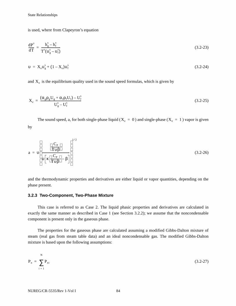
State Relationships
is used, where from Clapeyron’s equation
(3.2-23)
(3.2-24)
and is the equilibrium quality used in the sound speed formulas, which is given by
(3.2-25)
The sound speed, a, for both single-phase liquid ( ) and single-phase ( ) vapor is given
by
(3.2-26)
and the thermodynamic properties and derivatives are either liquid or vapor quantities, depending on the
phase present.
3.2.3 Two-Component, Two-Phase Mixture
This case is referred to as Case 2. The liquid phasic properties and derivatives are calculated in
exactly the same manner as described in Case 1 (see Section 3.2.2); we assume that the noncondensable
component is present only in the gaseous phase.
The properties for the gaseous phase are calculated assuming a modified Gibbs-Dalton mixture of
steam (real gas from steam table data) and an ideal noncondensable gas. The modified Gibbs-Dalton
mixture is based upon the following assumptions:
(3.2-27)
dPs
dT--------
hgs hf
s–
Ts υgs υ f
s–( )---------------------------=
υ Xeυgs 1 Xe–( )υ f
s+=
Xe
Xe
αgρgUg α fρfUf+( ) Ufs–
Ugs Uf
s–----------------------------------------------------------=
Xe 0= Xe 1=
a υ
CP
Tυβ-----------
υ κCP
Tυβ-----------
β–
---------------------------------------
1 2⁄
=
Pn Pni
i 1=
N
∑=
NUREG/CR-5535/Rev 1-Vol I 84

State Relationships
(3.2-28)
(3.2-29)
(3.2-30)
where and are the partial pressures of the steam and the individual noncondensable components,
respectively. The internal energies, , , and the specific volumes, , , are evaluated at the gas
temperature and the respective partial pressures. The vapor properties are obtained from the steam tables,
and the noncondensable state equations are
(3.2-31)
and
(3.2-32)
where
Rn = (3.2-33)
Co = (3.2-34)
Do = (3.2-35)
Uo = (3.2-36)
To = 250 K (3.2-37)
P Pn Ps+=
Ug XnUn 1 Xn–( )Us+=
υg Xnυn 1 Xn–( )υs= =
Ps Pni
Us Un υ s υn
Pnυn RnTg=
Un
Uo C+ oTg Tg To<
Uo C+ oTg12---Do Tg To–( )2 Tg To≥+
=
RniXni
i 1=
N
∑
Co ni, Xni
i 1=
N
∑
Do ni, Xni
i 1=
N
∑
Uo ni, Xni
i 1=
N
∑
85 NUREG/CR-5535/Rev 1-Vol I
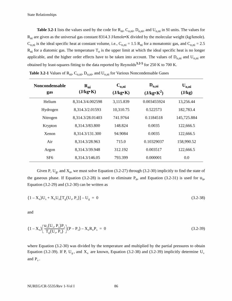
State Relationships
Table 3.2-1 lists the values used by the code for Rni, Co,ni, Do,ni, and Uo,ni in SI units. The values for
Rni are given as the universal gas constant 8314.3 J/kmole•K divided by the molecular weight (kg/kmole).
Co,ni is the ideal specific heat at constant volume, i.e., Co,ni = 1.5 Rni for a monatomic gas, and Co,ni = 2.5
Rni for a diatomic gas. The temperature To is the upper limit at which the ideal specific heat is no longer
applicable, and the higher order effects have to be taken into account. The values of Do,ni and Uo,ni are
obtained by least-squares fitting to the data reported by Reynolds3.2-5 for 250 K to 700 K.
Given P, Ug, and Xn, we must solve Equation (3.2-27) through (3.2-30) implicitly to find the state of
the gaseous phase. If Equation (3.2-28) is used to eliminate Pn, and Equation (3.2-31) is used for υn,
Equation (3.2-29) and (3.2-30) can be written as
(3.2-38)
and
(3.2-39)
where Equation (3.2-30) was divided by the temperature and multiplied by the partial pressures to obtain
Equation (3.2-39). If P, , and are known, Equation (3.2-38) and (3.2-39) implicitly determine
and .
Table 3.2-1 Values of Rni, Co,ni, Do,ni, and Uo,ni for Various Noncondensable Gases
Noncondensable gas
Rni(J/kg•K)
Co,ni
(J/kg•K)
Do,ni
(J/kg•K2)
Uo,ni
(J/kg)
Helium 8,314.3/4.002598 3,115.839 0.003455924 13,256.44
Hydrogen 8,314.3/2.01593 10,310.75 0.522573 182,783.4
Nitrogen 8,314.3/28.01403 741.9764 0.1184518 145,725.884
Krypton 8,314.3/83.800 148.824 0.0035 122,666.5
Xenon 8,314.3/131.300 94.9084 0.0035 122,666.5
Air 8,314.3/28.963 715.0 0.10329037 158,990.52
Argon 8,314.3/39.948 312.192 0.003517 122,666.5
SF6 8,314.3/146.05 793.399 0.000001 0.0
1 Xn–( )Us XnUn Tg Us Ps,( )[ ] Ug–+ 0=
1 Xn–( )υs Us Ps,( )Ps
Tg Us Ps,( )----------------------------- P Ps–( ) XnRnPs– 0=
Ug Xn Us
Ps
NUREG/CR-5535/Rev 1-Vol I 86

State Relationships
To obtain the derivatives needed in the numerical scheme, we must evaluate the derivatives of
and with respect to P, , and . These derivatives can be obtained from Equation (3.2-38) and (3.2-
39) by the use of the chain rule and implicit differentiation. For example, taking the derivative of Equation
(3.2-38) and (3.2-39) with respect to P [recall that and ], we
obtain
(3.2-40)
as a linear system of two equations determining
In Equation (3.2-40),
(3.2-41)
is the equivalent gas constant for the steam vapor,
(3.2-42)
and
(3.2-43)
To obtain the derivatives of and with respect to and , we repeat the above development
taking derivatives of Equation (3.2-38) and (3.2-39) with respect to and . In each case, linear
equations parallel to those in Equation (3.2-40) are obtained. In fact, the left side matrix is exactly the
same, and the right side vector changes.
Us
Ps Ug Xn
Ps Ps P Ug Xn, ,( )= Us Us P Ug Xn, ,( )=
Xn
dUn
dTg---------
∂Tg
∂Ps---------
Us
1 Xn– Xn
dUn
dTg---------
∂Tg
∂Us---------
Ps
+
XnRn– 1 Xn–( )Rs– TERM2
TERM1+
•
∂Ps
∂P--------
Ug Xn,
∂Us
∂P---------
Ug Xn,
0
1 Xn–( )– Rs
=
∂Ps
∂P--------
Ug Xn,
and ∂Us
∂P---------
Ug Xn,
Rs
Psυs
Tg----------=
TERM1 1 Xn–( )PnRs1Ps-----
1υs-----
∂υs
∂Ps--------
Us
1Tg-----
∂Tg
∂Ps---------
Us
–+=
TERM2 1 Xn–( )PnRs1υs-----
∂υ s
∂Us---------
Ps
1Tg-----
∂Tg
∂Us---------
Ps
–=
Ps Us Ug Xn
Ug Xn
87 NUREG/CR-5535/Rev 1-Vol I
State Relationships
Having obtained all the derivatives of and , it is relatively easy to obtain the temperature
derivatives needed for the gaseous phase. From the chain rule, we have
(3.2-44)
(3.2-45)
(3.2-46)
where
are the standard phasic derivatives for the vapor phase. Equation (3.2-44) through (3.2-46) give all the
desired gaseous temperature derivatives. The interface temperature derivatives are obtained from
Clapeyron’s equation and the known derivatives, i.e.,
(3.2-47)
(3.2-48)
(3.2-49)
where is given by the reciprocal of Equation (3.2-23).
The derivatives of the densities can be obtained from or , as these two
formulae for the gaseous specific volume are equivalent [see Equation (3.2-30)]. A symmetric formula can
be obtained by eliminating from the above two formulae, giving
Ps Us
∂Tg
∂P---------
Ug Xn,
∂Tg
∂Ps---------
Us
∂Ps
∂P--------
Ug Xn,
∂Tg
∂Us---------
Ps
∂Us
∂P---------
Ug Xn,
+=
∂Tg
∂Ug---------
P Xn,
∂Tg
∂Ps---------
Us
∂Ps
∂Ug---------
P Xn,
∂Tg
∂Us---------
Ps
∂Us
∂Ug---------
P Xn,
+=
∂Tg
∂Xn---------
P Ug,
∂Tg
∂Ps---------
Us
∂Ps
∂Xn---------
P Ug,
∂Tg
∂Us---------
Ps
∂Us
∂Xn---------
P Ug,
+=
∂Tg
∂Ps---------
Us
and ∂Tg
∂Us---------
Ps
Ps
∂TI
∂P--------
Ug X, n
dTI
dPs--------
∂Ps
∂P--------
Ug Xn,
=
∂TI
∂Ug---------
P X, n
dTI
dPs--------
∂Ps
∂Ug---------
P Xn,
=
∂TI
∂Xn---------
P U, g
dTI
dPs--------
∂Ps
∂Xn---------
P Ug,
=
dTI
dPs--------
υg Xnυn= υg 1 Xn–( )υs=
Xn
NUREG/CR-5535/Rev 1-Vol I 88
State Relationships
(3.2-50)
Using Equation (3.2-50), we have for the derivatives of with respect to P
(3.2-51)
Similar formulas are obtained when either or is the independent variable. The partial
derivatives on the right side of Equation (3.2-51) are obtained from formulae exactly parallel to those in
Equation (3.2-44) through (3.2-46) with replaced by or . When taking the derivatives of , we
use
(3.2-52)
Hence, an additional term appears in the parallel formula for Equation (3.2-44) due to the direct
dependence of on P.
The homogeneous equilibrium sound speed (a) for a noncondensable-steam-water mixture is3.2-2
taken from
(3.2-53)
where
(3.2-54)
(3.2-55)
υg
υsυn
υs υn+-----------------=
ρg
∂ρg
∂P--------
Ug X, n
1
υn2
-----∂υn
∂P--------
Ug Xn,
–1
υs2
-----∂υ s
∂P--------
Ug Xn,
–=
Ug Xn
Tg υs υn υn
vn
RnTg Ps υ s,( )P Ps–
------------------------------=
υn
a2 υ2
∂υ∂P------
S Xn,
–
------------------------=
∂υ∂P------
S Xn,
1 Xf–( ) Xn2υn βn
1P ′ s------ κn+
∂Ps
∂P--------
S Xn,
κn– Xs2υs βs
1P ′ s------ κ s–
∂Ps
∂P--------
S Xn,
+
=
Xfυ f βf1
P ′ s------
∂Ps
∂P--------
S Xn,
κ f– υg υ f–( ) ∂Xs
∂P---------
S Xn,
+ +
P ′ sdPs
dT--------
hss hf
s–
Ts υ ss υ f
s–( )--------------------------
Sss Sf
s–
υss υ f
s–----------------= ==
89 NUREG/CR-5535/Rev 1-Vol I

State Relationships
Equation (3.2-54) is similar to Equation (18) in Reference 3.2-2, where the relation
(3.2-56)
is used. Equation (3.2-55) is the inverse of Equation (22) (Clausius-Clapeyron relation) in Reference 3.2-
2. The quantities and in Equation (3.2-54) are obtained from the following matrix
equation
(3.2-57)
Equation (3.2-57) is from the first and third equations in Equation (19) in Reference 3.2-2, where
Equation (3.2-56) is used as well as
(3.2-58)
In the above formulae, , , , and are, respectively, mass qualities for steam,
noncondensable, gas, and liquid based on the total mixture mass; and are the mass qualities for
steam and noncondensable based on the gas mixture mass. Thus, their definitions are
(3.2-59)
(3.2-60)
(3.2-61)
∂T∂P------
S Xn,
1P ′ s------
∂Ps
∂P--------
S Xn,
=
∂Ps
∂P--------
S Xn,
∂Xs
∂P---------
S Xn,
Xnυnβn Xsυsβs– Ss Sf–
1
Ps’
----- XnCpn XsCps+( ) 1Tg----- XfCpf
1Tf-----+ +
Xnυn κn βn1
Ps’
-----+ Xsυs κ s βs–
1
Ps’
----- + υs–
∂Ps
∂P--------
S Xn,
∂Xs
∂P---------
S Xn,
•
Xnυnβn Xfυ fβf+
Xnυnκn
=
Xnυn Xsυs Xgυg= =
Xs Xn Xg Xf
Xs Xn
XsMs
Ms Mn Mf+ +----------------------------------=
XnMn
Ms Mn Mf+ +----------------------------------=
Xg XMs Mn+
Ms Mn Mf+ +----------------------------------
Mg
Mg Mf+--------------------= = =
NUREG/CR-5535/Rev 1-Vol I 90
State Relationships
(3.2-62)
(3.2-63)
(3.2-64)
where
= the mass of the steam in the gaseous phase
= the mass of the noncondensable in the gaseous phase
=the mass of the gaseous phase
= the mass of the liquid phase.
The variable is usually referred to as the static quality.
The liquid properties and derivatives are obtained as above for Case 1. To obtain the gaseous
properties, Equation (3.2-38) and (3.2-39) must be solved iteratively. A global Newton iteration in two
variables is used.3.2-6 The iteration variables are and . The steam table subroutine is called once
during each iteration to obtain all the needed steam vapor properties, and Equation (3.2-31) and (3.2-32)
are used to obtain the air properties. Once the iteration has converged, the gaseous properties are
determined from the formulas in this section.
The transport properties phasic viscosities µg, µf, phasic thermal conductivities kg, kf, and surface
tension σ are evaluated as functions of the local thermodynamic properties. Correlations from ASME3.2-3
and Schmidt3.2-7 are used for steam and liquid water. The presence of noncondensables in the vapor phase
is accounted for by using Wilke’s semi-empirical formula3.2-8 for µg, and by using Mason and Saxena’s
analogous method3.2-9 (with approved modification by Bird, Stewart, and Lightfoot3.2-10) for kg.
Evaluation of the sound speed formulas at the saturated equilibrium state requires a second iteration.
To avoid this extra iteration, the sound speed formulas were evaluated using the nonequilibrium state
properties.
XfMf
Ms Mn Mf+ +----------------------------------
Mf
Mg Mf+--------------------= =
Xs
Ms
Ms Mn+--------------------=
Xn
Mn
Ms Mn+--------------------=
Ms
Mn
Mg Ms Mn+=
Mf
X Xg=
Ps Us
91 NUREG/CR-5535/Rev 1-Vol I
State Relationships
3.2.4 References
3.2-1. J. G. Collier. Convective Boiling and Condensation, 2nd Edition. New York: McGraw-Hill.1981.
3.2-2. V. H. Ransom and J. A. Trapp. “Sound Speed Models for a Noncondensable Gas-Steam-WaterMixture.” Proceedings Japan-U.S. Seminar on Two-Phase Flow Dynamics. Lake Placid, NY.July 29-August 3, 1984.
3.2-3. American Society of Mechanical Engineers. Thermodynamic and Transport Properties of Steam.United Engineering Center, 345 East 45th Street, New York, NY. 1967.
3.2-4. P. W. Bridgman. Thermodynamics of Electrical Phenomena in Metals and a CondensedCollection of Thermodynamic Formulas. New York: Dover Publications. 1961.
3.2-5. W. C. Reynolds. Thermodynamic Properties in SI. Stanford University. 1979.
3.2-6. J. Dennis and R. Schnabel. Quasi-Newton Methods for Unconstrained Nonlinear Problems.Prentice-Hall. 1983.
3.2-7. E. Schmidt. Properties of Water and Steam in SI Units. New York: Springer-Verlag. 1969.
3.2-8. C. R. Wilke. “A Viscosity Equation for Gas Mixtures.” J. Chem Physics. 18. 1950. pp. 517-519.
3.2-9. E. A. Mason and S. C. Saxena. “Approximate Formula for the Thermal Conductivity of GasMixtures.” The Physics of Fluid. 1. 1958. pp. 361-369.
3.2-10. R. B. Bird. W. E. Stewart. and E. N. Lightfoot. Transport Properties. New York: Wiley and Sons.1960.
NUREG/CR-5535/Rev 1-Vol I 92

Constitutive Models
3.3 Constitutive Models
The constitutive relations include models for defining flow regimes and flow-regime-related models
for interphase drag and shear, the coefficient of virtual mass, wall friction, wall heat transfer, interphase
heat and mass transfer, and direct (sensible) heat transfer. Heat transfer regimes are defined and used for
wall heat transfer. For the virtual mass, a formula based on the void fraction is used.
In RELAP5/MOD2, all constitutive relations were evaluated using volume-centered conditions;
junction parameters, such as interfacial friction coefficients, were obtained as volume-weighted averages
of the volume-centered values in the volumes on either side of a junction. The procedure for obtaining
junction parameters as averages of volume parameters was adequate when the volumes on either side of a
junction were in the same flow regime and the volume parameters were obtained using the same flow
regime map (i.e., both volumes were horizontal volumes or both volumes were vertical volumes).
Problems were encountered when connecting horizontal volumes to vertical volumes.
These problems have been eliminated in RELAP5/MOD3 by computing the junction interfacial
friction coefficient using junction properties so that the interfacial friction coefficient would be consistent
with the state of the fluid being transported through the junction. The approach has been used successfully
in the TRAC-B code.3.3-1,3.3-2 The independent variables in the flow regime maps for the volumes and
junctions are somewhat different as a result of the finite-difference scheme and staggered mesh used in the
numerical scheme.
The volume and junction flow regime maps will be discussed separately, followed by a discussion of
the interphase drag and shear, coefficient of virtual mass, wall friction, wall heat transfer models,
interphase heat and mass transfer, and direct (sensible) heat transfer. Volume I presents an overview of the
constitutive models, and Volume IV presents more details of the constitutive models.
The volume map is based on volume quantities. It is used for interphase heat and mass transfer, wall
friction, and wall heat transfer. The constitutive relations, in general, include flow regime effects for which
simplified mapping techniques have been developed to control the use of constitutive relation correlations.
The flow regime maps are based on the work of Taitel and Dukler3.3-3,3.3-4 and Ishii.3.3-5,3.3-6,3.3-7
Taitel and Dukler have simplified flow regime classifications and developed semi-empirical relations
to describe flow regime transitions. However, some of their transition criteria are quite complex, and
further simplification has been carried out in order to efficiently apply these criteria in RELAP5. In
addition, post-critical heat flux (CHF) regimes as suggested by Ishii3.3-5 are included.
Four flow regime maps are used: a horizontal map for flow in pipes; a vertical map for flow in pipes,
annuli, and bundles; a high mixing map for flow in pumps; and an ECC mixer map for flow in the
horizontal pipe near the ECC injection port.
93 NUREG/CR-5535/Rev 1-Vol I

Constitutive Models
3.3.1 Vertical Volume Flow Regime Map
The vertical flow regime map (for both up and down flow) is for volumes whose elevation angle φ is
such that 45 < |φ| < 90 degrees. This map is modeled as nine regimes--four for pre-CHF heat transfer, four
for post-CHF heat transfer, and one for vertical stratification. For pre-CHF heat transfer, the regimes
modeled are the bubbly, slug, annular-mist, and mist-pre-CHF regimes. Formulations for the first three
regimes were utilized by Vince and Lahey3.3-8 to analyze their data. The mist-pre-CHF regime was added
for smoothness. For post-CHF heat transfer, the bubbly, slug, and annular-mist regimes are transformed to
the inverted annular, inverted slug, and mist regimes, respectively, as suggested by Ishii.3.3-5 The mist-
post-CHF regime was added for symmetry with the mist-pre-CHF regime. The mist flow regimes consist
of pure droplet flow where all of the available liquid is assumed to be entrained and there is no liquid film
on the wall. Unheated components are also modeled, utilizing the pre-CHF map. A schematic representing
the pre-CHF, post-CHF, and transition regimes of the vertical flow regime map is shown in Figure 3.3-1.
The schematic is three-dimensional, to illustrate flow regime transitions as functions of void fraction αg,
average mixture velocity vm, and boiling regime (pre-CHF, transition, and post-dryout) where
(3.3-1)
(3.3-2)
(3.3−3)
The map consists of bubbly, slug, annular-mist, and dispersed (droplet or mist) flows in the pre-CHF
regime; inverted annular, inverted slug, and dispersed (droplet or mist) flows in post-dryout; and vertically
stratified for sufficiently low mixture velocity vm. Transition regions provided in the code are shown. The
flow regime identifiers which appear in the printed output are shown in parenthesis for each of the regimes.
The criteria for defining the boundaries for transition from one regime to another are given by the
following correlations.
For the bubbly-to-slug transition, Taitel and Dukler3.3-3,3.3-4 suggested that bubbly flow may not
exist in tubes of small diameter where the rise velocity of small bubbles exceeds the rise velocity of Taylor
bubbles. The small bubble rise velocity is given by the correlation3.3-4
(3.3-4)
and the Taylor bubble rise velocity is given by the correlation3.3-9
vm
Gm
ρm-------=
Gm α gρg vg α fρf vf+=
ρm αgρg α fρf+=
vsb 1.53g ρf ρg–( )σ
ρf2
----------------------------1 4⁄
1.53D*σDρf----------
1 2⁄
= =
NUREG/CR-5535/Rev 1-Vol I 94

Constitutive Models
(3.3-5)
(Note: in Reference 3.3-4, is approximated as ; see also Reference 3.3-6 and Reference
3.3-10.) Accordingly, the limiting dimensionless tube diameter allowing the presence of bubbly flow is
(3.3-6)
where is the dimensionless tube diameter,
(3.3-7)
In the coding, 19.11 has been modified to 22.22 where this value was chosen based on comparisons
with data during the developmental assessment of RELAP5/MOD2.3.3-11 This is discussed further in
Volume IV of this manual.
Figure 3.3-1 Schematic of Vertical Flow Regime Map with Hatchings Indicating Transitions
Vertically stratified (VST)
Transition
Unstratified
Bubbly(BBY)
SLG/ANM
Annularmist (ANM)
Slug(SLG)
Mist(MST)
Invertedslug (ISL)
IAN/ISL
BBY/IAN
Invertedannular
IAN/ISL-
SLG
ISL-SLG/
ANM
Post-dryout
Transition
Pre-CHF
vTb
αBS αSA αAM
Increasingvm
αBS αSA
(MPR
)
(MPO
)
SLG/ISL ANM/MST
(IAN)
1.00.0
Increasing αg
0.0 1.0αAM
αDE
αCD
Incr
easi
ng T
g -
Ts
12
vTb
vTb 0.35gD ρf ρg–( )
ρf-----------------------------
1 2⁄0.35D* σ
Dρf---------
1 2⁄= =
ρf ρg– ρf
D* 19.11≥
D*
D* Dg ρf ρg–( )
σ------------------------
1 2⁄
=
95 NUREG/CR-5535/Rev 1-Vol I

Constitutive Models
Equation (3.3-7) is the dimensionless ratio of tube diameter to film thickness times the Deryagin
number, where the Deryagin number is the ratio of film thickness to capillary length. Also, in the limit, as
the fluid properties approach the thermodynamic critical pressure, D* = D.
For tubes with diameters satisfying the condition of Equation (3.3-6), the bubble-slug transition
occurs at a void fraction αg = 0.25 for low mass fluxes of G ≤ 2000 kg/m2•s. By combining this void
criterion with Equation (3.3-6) and using 22.22 instead of 19.11, the bubble-slug transition criterion can be
defined such that
(3.3-8)
Hence, if the local void fraction, αg, exceeds the criterion of Equation (3.3-8), then bubbly flow
cannot exist, since the rise velocity of small bubbles exceeds that of Taylor bubbles. The exponential
power of 8 is used to provide a smooth variation of αL as D* decreases.
At high mass fluxes of Gm ≥ 3000 kg/m2•s, bubbly flow with finely dispersed bubbles can exist up to
a void fraction, αg, of 0.5. Then, if the criterion is linearly interpolated between the upper and lower void
limits, the bubbly-slug transition criterion can be written as
(3.3−9)
for mass fluxes of Gm < 2000 kg/m2•s,
(3.3−10)
for mass fluxes of 2000. < Gm < 3000 kg/m2•s, and
(3.3−11)
for mass fluxes of Gm ≥ 3000 kg/m2 s. The flow regime can therefore be said to be in the bubbly regime if
αg < αBS and in the slug regime if αg ≥ αBS.
The bubble-slug transition defined by Equation (3.3-9) to (3.3-11) is similar to that given by Taitel
and Dukler,3.3-4 except that their void fraction relation is converted into a form based on liquid and vapor
superficial velocities, and finely dispersed bubbles are also distinguished from ordinary bubbles.
α 0.25 min 1.0D*
22.22-------------
8
,=
αBS αL=
αBS αL 0.001 0.5 αL–( ) Gm 2000–( )+=
αBS 0.5=
NUREG/CR-5535/Rev 1-Vol I 96

Constitutive Models
For the slug to annular transition, Taitel et al.3.3-4 and Mishima and Ishii3.3-12 indicate that the
annular flow transition for upflow is principally governed by criteria of the form
(3.3-12)
and
(3.3-13)
with the first criterion (flow reversal) controlling the transition in small tubes and the second criterion
(droplet entrainment) controlling the transition in large tubes. McQuillan and Whalley3.3-13,3.3-14
considered the above criteria using
(3.3-14)
and
(3.3-15)
and obtained good predictions of the annular flow boundary in each case. Putney3.3-15 has found that better
agreement can be obtained if annular flow occurs when either criterion is satisfied. In terms of the slug-to-
annular transition void fraction αSA, Putney indicates that these criteria take on the form
(3.3-16)
where
= for upflow (3.3-17)
= 0.75 for downflow and countercurrent flow (3.3-18)
jg* αgvg
gDρf ρg–( )
ρg---------------------
1 2⁄----------------------------------------- jg crit,*≥=
Kug
αgvg
gσρf ρg–( )
ρg2
---------------------1 4⁄---------------------------------------- Kug crit,≥=
jg crit,* 1=
Kug crit, 3.2=
αSA min α critf α crit
e,( )=
α critf 1
vg-----
gD ρf ρg–( )ρg
-----------------------------1 2⁄
97 NUREG/CR-5535/Rev 1-Vol I

Constitutive Models
and
(3.3-19)
where the void fraction for flow reversal, , is found by combining Equation (3.3-12) and (3.3-14) and
the void fraction for droplet entrainment, , is found by combining Equation (3.3-13) and (3.3-15).
The transition region between the slug flow and annular mist flow regimes is defined by αDE and
αSA where
(3.3−20)
The minimum void fraction for annular mist flow, αSA, is constrained to lie between 0.5 and 0.9.
For the transition between annular mist and mist pre-CHF (regime MPR in Figure 3.3-1), the value
of αAM is
(3.3−21)
where all of the available liquid is assumed to be in the form of droplets in the mist regimes.
If the hydrodynamic volume has heat flux from a surrounding wall to the vapor or the reflood model
is turned on for that wall, and the vapor temperature is more than 1 oK superheated, then the flow regime is
a post-CHF regime. For post-CHF heat transfer, the above formulations are also used to define the
regimes. Equation (3.3-9) through (3.3-11) define the inverted annular to inverted slug regime transition,
Equation (3.3-16) defines the inverted slug to mist regime transition, and Equation (3.3-21) defines the
mist to mist post-CHF (regime MPO in Figure 3.3-1) regime transition. The transition region between
inverted slug flow and inverted annular flow regimes is defined by αΒS and αCD where
(3.3−22)
At low mass fluxes, the possibility exists for vertically stratified conditions. In RELAP5, vertical
flow in a volume cell is considered to be stratified if the following criteria are met:
• The void fraction for the volume above is > 0.7, and the difference between the voidfractions in the volume in question and the void fraction in the volume above or below is
α crite 3.2
vg-------
gσ ρf ρg–( )ρg
2----------------------------
1 4⁄=
α critf
α critf
αDE max αBS αSA 0.05–,( )=
αAM 0.9999=
αCD αBS 0.2+=
NUREG/CR-5535/Rev 1-Vol I 98
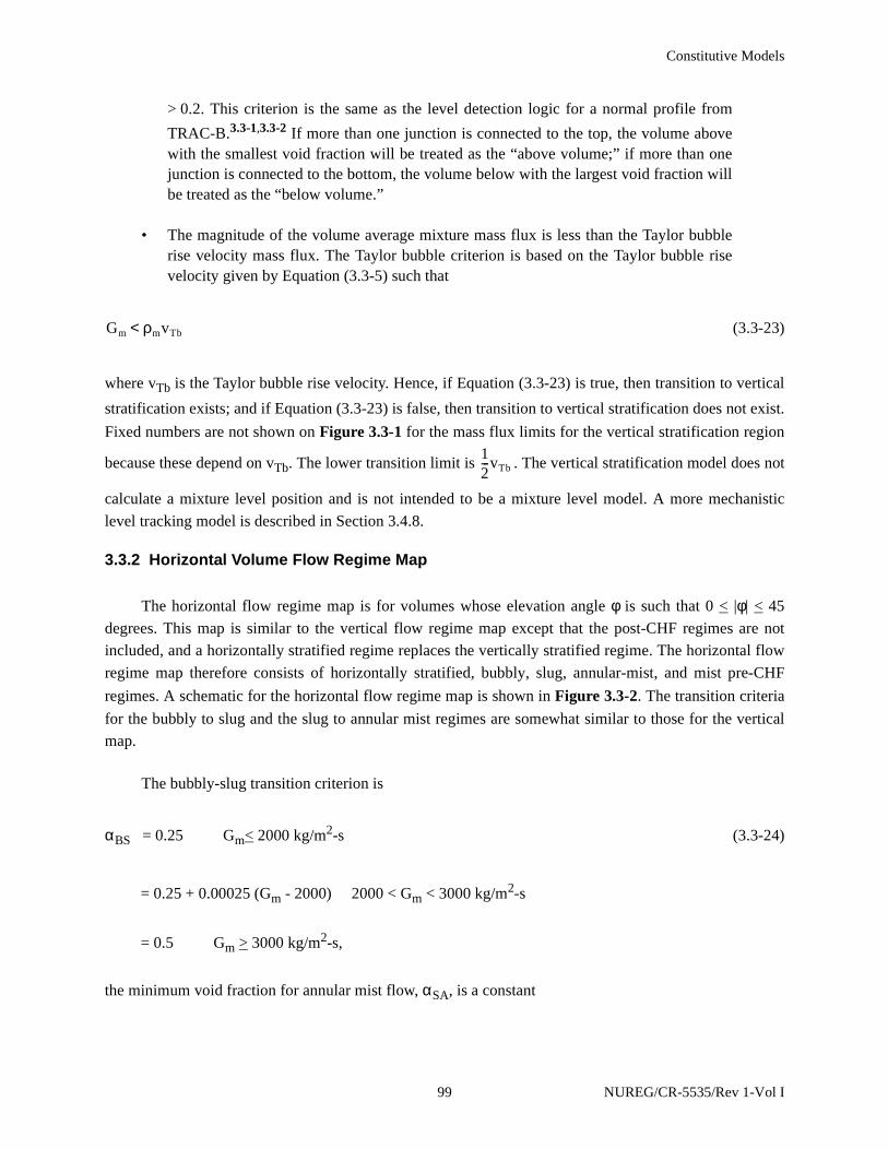
Constitutive Models
> 0.2. This criterion is the same as the level detection logic for a normal profile from
TRAC-B.3.3-1,3.3-2 If more than one junction is connected to the top, the volume abovewith the smallest void fraction will be treated as the “above volume;” if more than onejunction is connected to the bottom, the volume below with the largest void fraction willbe treated as the “below volume.”
• The magnitude of the volume average mixture mass flux is less than the Taylor bubblerise velocity mass flux. The Taylor bubble criterion is based on the Taylor bubble risevelocity given by Equation (3.3-5) such that
(3.3-23)
where vTb is the Taylor bubble rise velocity. Hence, if Equation (3.3-23) is true, then transition to vertical
stratification exists; and if Equation (3.3-23) is false, then transition to vertical stratification does not exist.
Fixed numbers are not shown on Figure 3.3-1 for the mass flux limits for the vertical stratification region
because these depend on vTb. The lower transition limit is . The vertical stratification model does not
calculate a mixture level position and is not intended to be a mixture level model. A more mechanistic
level tracking model is described in Section 3.4.8.
3.3.2 Horizontal Volume Flow Regime Map
The horizontal flow regime map is for volumes whose elevation angle φ is such that 0 < |φ| < 45
degrees. This map is similar to the vertical flow regime map except that the post-CHF regimes are not
included, and a horizontally stratified regime replaces the vertically stratified regime. The horizontal flow
regime map therefore consists of horizontally stratified, bubbly, slug, annular-mist, and mist pre-CHF
regimes. A schematic for the horizontal flow regime map is shown in Figure 3.3-2. The transition criteria
for the bubbly to slug and the slug to annular mist regimes are somewhat similar to those for the vertical
map.
The bubbly-slug transition criterion is
αBS = 0.25 Gm< 2000 kg/m2-s (3.3-24)
= 0.25 + 0.00025 (Gm - 2000) 2000 < Gm < 3000 kg/m2-s
= 0.5 Gm > 3000 kg/m2-s,
the minimum void fraction for annular mist flow, αSA, is a constant
Gm ρmvTb<
12---vTb
99 NUREG/CR-5535/Rev 1-Vol I
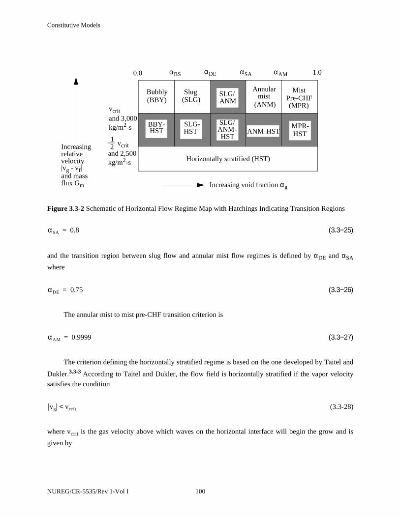
Constitutive Models
(3.3−25)
and the transition region between slug flow and annular mist flow regimes is defined by αDE and αSA
where
(3.3−26)
The annular mist to mist pre-CHF transition criterion is
(3.3−27)
The criterion defining the horizontally stratified regime is based on the one developed by Taitel and
Dukler.3.3-3 According to Taitel and Dukler, the flow field is horizontally stratified if the vapor velocity
satisfies the condition
(3.3-28)
where vcrit is the gas velocity above which waves on the horizontal interface will begin the grow and is
given by
Figure 3.3-2 Schematic of Horizontal Flow Regime Map with Hatchings Indicating Transition Regions
Horizontally stratified (HST)
Increasing void fraction αg
BBY-HST
SLG-HST
SLG/ANM-HST
ANM-HSTMPR-HST
Mist
(MPR)
Annularmist
(ANM)
SLG/ANM
Slug(SLG)
Bubbly(BBY)
vcrit
Increasingrelativevelocity|vg - vf|
αBS αSA αAM0.0 1.0αDE
and massflux Gm
and 2,500kg/m2-s
and 3,000kg/m2-s
Pre-CHF
21
vcrit
αSA 0.8=
αDE 0.75=
αAM 0.9999=
vg vcrit<
NUREG/CR-5535/Rev 1-Vol I 100

Constitutive Models
(3.3-29)
where θ is given by the solution of Equation (3.1-59). The angle θ (see Figure 3.1-2) is related to the liquid
level with respect to the bottom of the volume.
This condition is modified in the code to handle situations where the flow is stratified but the liquid is
not stagnant as was assumed by Taitel and Dukler.3.3-3 The flow is horizontally stratified if the phasic
velocity difference satisfies the condition
(3.3-30)
and the mass flux satisfies the condition
kg/m2-s (3.3-31)
If the horizontal stratification conditions of Equation (3.3-30) and (3.3-31) are met, then the flow
field undergoes a transition to the horizontally stratified flow regime. If the conditions of Equation (3.3-30)
and (3.3-31) are not met, then the flow field undergoes a transition to the bubbly, slug, annular mist, or
mist pre-CHF flow regime. The lower transition limit for |vg - vf| is (1/2) vcrit and for Gm is 2500 kg/m2-s.
3.3.3 High Mixing Volume Flow Regime Map
The high mixing flow regime map (used in pumps) is based on vapor void fraction, αg, and consists
of a bubbly regime for αg < 0.5, a mist regime for αg > 0.95, and a transition regime for 0.5 < αg < 0.95.
The transition regime is modeled as a mixture of bubbles dispersed in liquid and droplets dispersed in
vapor. A schematic for the high mixing flow regime map is shown in Figure 3.3-3.
3.3.4 ECC Mixer Volume Flow Regime Map
Prior to the introduction of the ECCMIX component into RELAP5/MOD3, RELAP5 included the
three previously discussed flow regime maps, as described in the RELAP5/MOD2 manual3.3-16 and in the
RELAP5/MOD2 models and correlations report.3.3-17 None of those, however, would apply specifically to
the condensation process in a horizontal pipe near the emergency core coolant (ECC) injection port. A
flow regime map for condensation inside horizontal tubes is reported by Tandon et al.,3.3-18 and it was
considered a more suitable basis for the interfacial heat transfer calculation in condensation for this
geometry. According to Reference 3.3-18, the two-phase flow patterns during condensation inside a
vcrit12---
ρf ρg–( )gαgAρgD θsin
-----------------------------------
12---
1 θcos–( )=
vg vf– vcrit<
Gm 3000<
101 NUREG/CR-5535/Rev 1-Vol I

Constitutive Models
horizontal pipe may be identified in terms of the local volumetric ratio of liquid and vapor, , and the
nondimensional vapor velocity, , where
=
Xf =
G =
and D is the diameter of the channel.
Although the condensation flow regime map of Tandon et al.3.3-18 does not include any zone for
bubbly flow, the existence of a bubbly flow regime at very low void fractions cannot be logically excluded,
particularly in a highly turbulent liquid flow. For this reason, a region of bubbly flow was included for void
fractions less than 20% (αg < 0.2). Furthermore, to protect against failure of the numerical solution, it is
necessary to specify some reasonable flow pattern for every combination of the volumetric ratio and . It
is also necessary to include transition zones around some of the boundaries between different flow
patterns. The transition zones are needed for interpolation between the calculated values of the correlations
for the interfacial heat transfer and friction that apply for the different flow patterns. These interpolations
prevent discontinuities that would otherwise exist and that could make the numerical solutions very
difficult. With these considerations, the flow regime map of Reference 3.3-18 was modified, as shown in
Figure 3.3-4. The modified condensation flow regime map comprises eleven different zones that include
six basic patterns and five interpolation zones. Table 3.3-1 shows a list of the basic flow patterns and the
Figure 3.3-3 Schematic of High Mixing Volume Flow Regime Map
Bubbly(CTB)
Mist(CTM)
0.500.0 1.00.95Increasing void fraction αg
Transition
(CTT)
1 α g–αg
--------------
vg*
vg* XfG
gDρg ρf ρg–( )[ ] 1 2⁄----------------------------------------------
α gρgvg
αgρgvg α fρfvf+--------------------------------------
α gρgvg α fρfvf+
vg*
NUREG/CR-5535/Rev 1-Vol I 102

Constitutive Models
interpolation zones for the ECCMIX component, with their acronyms and flow regime numbers, that are
printed out in the RELAP5/MOD3 output.
Figure 3.3-4 Schematic of ECC Mixer Volume Flow Regime Map (modified Tandon et al.)
Table 3.3-1 List of Flow Regimes in the ECCMIX Component
Flow regime
numberaFlow regime Acronym Remarks
16a Wavy MWY Basic pattern
17 Wavy/annular mist MWA Transition between wavy and annular mist flows
18 Annular mist MAM Basic pattern
19 Mist MMS Basic pattern
20 Wavy/slug MWS Transition between wavy and slug flows
21 Wavy/plug/slug MWP Transition between wavy, plug, and slug flows
0.001 0.1 1 10 100 100010-3
10-2
10-1
100
101
102
Bubbly (MBB)Plug
Wavy (MWY)
Slug
Annular mist (MAM)
Mist (MMS)
√g Dρg∆ρ
(MPL)
(MSL)
Liquid-to-vapor volumetric ratio, 1-αgαg
* GXf vg =
Dim
ensi
onle
ss g
as v
eloc
ity,
vg*
0.01
103 NUREG/CR-5535/Rev 1-Vol I

Constitutive Models
The variable names that are used in the coding for the coordinates of the condensation flow regime
map are
(3.3-32)
(3.3-33)
In terms of these variables, the different zones of the flow regime map are:
If voider > 4.0, bubbly flow, MBB
If 3.0 < voider < 4.0 and stargj < 0.01, transition, MPB
If 0.5 < voider < 4.0 and stargj > 0.0125, slug flow, MSL
If 0.625 < voider < 4.0, and 0.01 < stargj < 0.0125, transition, MPS
If 0.5 < voider < 3.0, and stargj < 0.01, plug flow, MPL
If 0.5 < voider < 0.625, and 0.01 < stargj < 0.0125, transition, MWP
If 0.5 < voider < 0.625, and 0.0125 < stargj < 1.0, transition, MWS
22 Plug MPL Basic pattern
23 Plug/slug MPS Transition between plug and slug flows
24 Slug MSL Basic pattern
25 Plug/bubbly MPB Transition between plug and bubbly flows
26 Bubbly MBB Basic pattern
a. Flow regime numbers 1 through 15 are used in RELAP5 for flow patterns in other components.
Table 3.3-1 List of Flow Regimes in the ECCMIX Component (Continued)
Flow regime
numberaFlow regime Acronym Remarks
voider1 αg–
αg--------------=
st jarg vg* XfG
gDρg ρf ρg–( )[ ] 1 2⁄----------------------------------------------= =
NUREG/CR-5535/Rev 1-Vol I 104
Constitutive Models
If voider < 0.5 and stargj < 1.0, wavy flow, MWY
If voider < 0.5, and 1.0 < stargj < 1.125, transition, MWA
If voider < 0.5, and 1.125 < stargj < 6.0, annular mist, MAM
If voider < 0.5, and stargj > 6.0, mist flow, MMS
In the coding, each one of these regions is identified by a flow pattern identification flag, MFLAG,
whose value varies from 1 for wavy flow to 11 for bubbly flow. The flow regime number in Table 3.3-1 is
MFLAG + 15.
In addition to the transition zones that are shown on Figure 3.3-4 and listed in Table 3.3-1, there are
two other transitions, namely:
• Transition between wavy and plug flows
• Transition between annular mist and mist (or droplet) flows
Interpolations between the interfacial friction, interfacial heat transfer, and the wall friction rates for
these transitions are performed through the gradual changes in the interfacial area in the first case and the
droplet entrainment fraction in the second case. Hence, there was no need for specifying transition zones
for these on the flow regime map.
3.3.5 Junction Flow Regime Map
The junction map is based on both junction and volume quantities. It is used for the interphase drag
and shear, as well as the coefficient of virtual mass. The flow regime maps used for junctions are the same
as used for the volumes and are based on the work of Taitel and Dukler,3.3-3,3.3-4,3.3-19 Ishii,3.3-5,3.3-7 and
Tandon et al.3.3-18
Junction quantities used in the map decisions are junction phasic velocities, donored (based on phasic
velocities) phasic densities, and donored (based on mixture superficial velocity) surface tension.
The junction void fraction, , is calculated from either of the volume void fractions of the
neighboring volumes, αg,K or αg,L, using a donor direction based on the mixture superficial velocity, jm. A
cubic spline weighting function is used to smooth the void fraction discontinuity across the junction when
|jm| < 0.465 m/s. The purpose of this method is to use a void fraction that is representative of the real
junction void fraction. This is assumed to have the form
(3.3-34)
αg j,*
αg j,* wj αg K,• 1 wj–( ) α g L,•+=
105 NUREG/CR-5535/Rev 1-Vol I
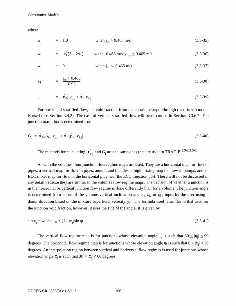
Constitutive Models
where
wj = 1.0 when jm > 0.465 m/s (3.3-35)
wj = when -0.465 m/s < jm < 0.465 m/s (3.3-36)
wj = 0 when jm < -0.465 m/s (3.3-37)
x1 = (3.3-38)
jm = (3.3-39)
For horizontal stratified flow, the void fraction from the entrainment/pullthrough (or offtake) model
is used (see Section 3.4.2). The case of vertical stratified flow will be discussed in Section 3.3.6.7. The
junction mass flux is determined from
(3.3-40)
The methods for calculating and Gj are the same ones that are used in TRAC-B.3.3-1,3.3-2
As with the volumes, four junction flow regime maps are used. They are a horizontal map for flow in
pipes; a vertical map for flow in pipes, annuli, and bundles; a high mixing map for flow in pumps; and an
ECC mixer map for flow in the horizontal pipe near the ECC injection port. These will not be discussed in
any detail because they are similar to the volumes flow regime maps. The decision of whether a junction is
in the horizontal or vertical junction flow regime is done differently than for a volume. The junction angle
is determined from either of the volume vertical inclination angles, φK or φL, input by the user using a
donor direction based on the mixture superficial velocity, jm. The formula used is similar to that used for
the junction void fraction, however, it uses the sine of the angle. It is given by
sin φj = wj sin φK + (1 - wj)sin φL (3.3-41)
The vertical flow regime map is for junctions whose elevation angle φj is such that 60 < |φj| < 90
degrees. The horizontal flow regime map is for junctions whose elevation angle φj is such that 0 < |φj| < 30
degrees. An interpolation region between vertical and horizontal flow regimes is used for junctions whose
elevation angle φj is such that 30 < |φj| < 60 degrees.
x12 3 2x1–( )
jm 0.465+0.93
------------------------
α· g j, vg j, α· f j, vf j,+
Gj α· g j, ρ· g j, vg j, α· f j, ρ· f j, vf j,+=
αg j,*
NUREG/CR-5535/Rev 1-Vol I 106
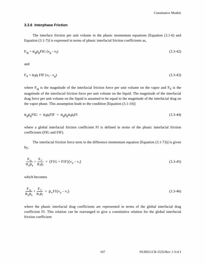
Constitutive Models
3.3.6 Interphase Friction
The interface friction per unit volume in the phasic momentum equations [Equation (3.1-6) and
Equation (3.1-7)] is expressed in terms of phasic interfacial friction coefficients as,
Fig = αgρgFIG (vg - vf) (3.3-42)
and
Fif = αfρf FIF (vf - vg) (3.3-43)
where Fig is the magnitude of the interfacial friction force per unit volume on the vapor and Fif is the
magnitude of the interfacial friction force per unit volume on the liquid. The magnitude of the interfacial
drag force per unit volume on the liquid is assumed to be equal to the magnitude of the interfacial drag on
the vapor phase. This assumption leads to the condition [Equation (3.1-10)]
αgρgFIG = αfρfFIF = αgρgαfρfFI (3.3-44)
where a global interfacial friction coefficient FI is defined in terms of the phasic interfacial friction
coefficients (FIG and FIF).
The interfacial friction force term in the difference momentum equation [Equation (3.1-73)] is given
by,
(3.3-45)
which becomes
(3.3-46)
where the phasic interfacial drag coefficients are represented in terms of the global interfacial drag
coefficient FI. This relation can be rearranged to give a constitutive relation for the global interfacial
friction coefficient
Fig
α gρg-----------
Fif
α fρf----------+ FIG FIF+( ) vg vf–( )=
Fig
αgρg-----------
Fif
α fρf----------+ ρmFI vg vf–( )=
107 NUREG/CR-5535/Rev 1-Vol I
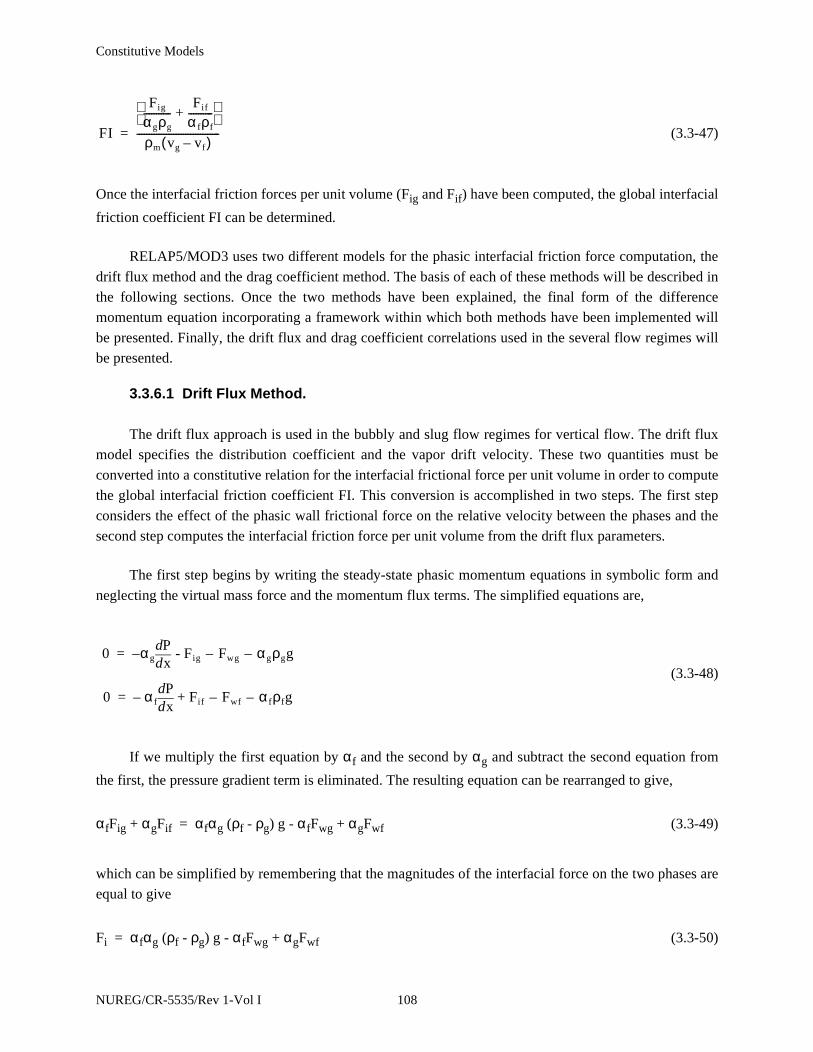
Constitutive Models
(3.3-47)
Once the interfacial friction forces per unit volume (Fig and Fif) have been computed, the global interfacial
friction coefficient FI can be determined.
RELAP5/MOD3 uses two different models for the phasic interfacial friction force computation, the
drift flux method and the drag coefficient method. The basis of each of these methods will be described in
the following sections. Once the two methods have been explained, the final form of the difference
momentum equation incorporating a framework within which both methods have been implemented will
be presented. Finally, the drift flux and drag coefficient correlations used in the several flow regimes will
be presented.
3.3.6.1 Drift Flux Method.
The drift flux approach is used in the bubbly and slug flow regimes for vertical flow. The drift flux
model specifies the distribution coefficient and the vapor drift velocity. These two quantities must be
converted into a constitutive relation for the interfacial frictional force per unit volume in order to compute
the global interfacial friction coefficient FI. This conversion is accomplished in two steps. The first step
considers the effect of the phasic wall frictional force on the relative velocity between the phases and the
second step computes the interfacial friction force per unit volume from the drift flux parameters.
The first step begins by writing the steady-state phasic momentum equations in symbolic form and
neglecting the virtual mass force and the momentum flux terms. The simplified equations are,
(3.3-48)
If we multiply the first equation by αf and the second by αg and subtract the second equation from
the first, the pressure gradient term is eliminated. The resulting equation can be rearranged to give,
αfFig + αgFif = αfαg (ρf - ρg) g - αfFwg + αgFwf (3.3-49)
which can be simplified by remembering that the magnitudes of the interfacial force on the two phases are
equal to give
Fi = αfαg (ρf - ρg) g - αfFwg + αgFwf (3.3-50)
FI
Fig
αgρg-----------
Fif
α fρf----------+
ρm vg vf–( )----------------------------------=
0 αg xddP
– - Fig Fwg– αg– ρgg=
0 α f xddP
– Fif Fwf – α f– ρfg+=
NUREG/CR-5535/Rev 1-Vol I 108
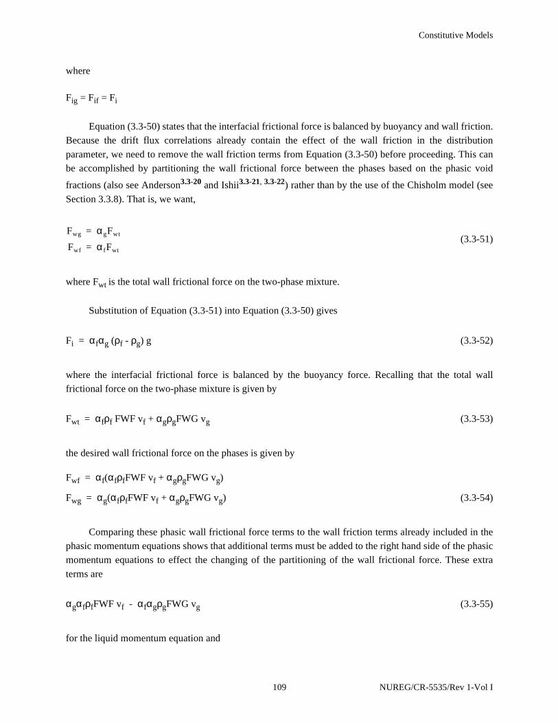
Constitutive Models
where
Fig = Fif = Fi
Equation (3.3-50) states that the interfacial frictional force is balanced by buoyancy and wall friction.
Because the drift flux correlations already contain the effect of the wall friction in the distribution
parameter, we need to remove the wall friction terms from Equation (3.3-50) before proceeding. This can
be accomplished by partitioning the wall frictional force between the phases based on the phasic void
fractions (also see Anderson3.3-20 and Ishii3.3-21, 3.3-22) rather than by the use of the Chisholm model (see
Section 3.3.8). That is, we want,
(3.3-51)
where Fwt is the total wall frictional force on the two-phase mixture.
Substitution of Equation (3.3-51) into Equation (3.3-50) gives
Fi = αfαg (ρf - ρg) g (3.3-52)
where the interfacial frictional force is balanced by the buoyancy force. Recalling that the total wall
frictional force on the two-phase mixture is given by
Fwt = αfρf FWF vf + αgρgFWG vg (3.3-53)
the desired wall frictional force on the phases is given by
Fwf = αf(αfρfFWF vf + αgρgFWG vg)
Fwg = αg(αfρfFWF vf + αgρgFWG vg) (3.3-54)
Comparing these phasic wall frictional force terms to the wall friction terms already included in the
phasic momentum equations shows that additional terms must be added to the right hand side of the phasic
momentum equations to effect the changing of the partitioning of the wall frictional force. These extra
terms are
αgαfρfFWF vf - αfαgρgFWG vg (3.3-55)
for the liquid momentum equation and
Fwg α gFwt=
Fwf α fFwt=
109 NUREG/CR-5535/Rev 1-Vol I

Constitutive Models
- αgαfρfFWF vf + αfαgρgFWG vg (3.3-56)
for the vapor momentum equation. These terms can be simplified by defining,
(3.3-57)
so that the extra terms in the liquid momentum equations can be written as,
fwf vf - fwg vg (3.3-58)
and for the vapor momentum equations as
fwg vg - fwf vf (3.3-59)
A means of removing the extra terms when the interfacial frictional force model is not being
determined from the drift flux correlations has been implemented by multiplying the extra terms by a
parameter fx which is defined as fx = 1 when the drift flux model is being used to determine the interfacial
friction force and is defined as fx = 0 when the drag coefficient model is being used to determine the
interfacial friction force. This parameter is interpolated from one to zero in the interpolation region
between flow regimes using the drift flux model and those using the two-fluid model for the determination
of the interfacial force term.
The interfacial force relation specified by Equation (3.3-52) does not constitute a constitutive relation
for the interfacial force since it does not provide a relationship between the interfacial force and the relative
velocity. Such a relation can be found by assuming that the interfacial force is given by,
Fi = Ci |vR|vR (3.3-60)
where Ci is a unknown coefficient and vR is the relative velocity between the phases. Within the context of
the drift flux model, the relative velocity between the phases in not the difference between the phasic
velocities but is a weighted difference between the phase velocities given by,
vR = C1vg - C0vf (3.3-61)
where C0 is given by the drift flux correlation and C1 is given by
fwg α fαgρgFWG=
fwf αgα fρfFWF=
NUREG/CR-5535/Rev 1-Vol I 110
Constitutive Models
(3.3-62)
Substituting these relations into Equation (3.3-60) gives the interfacial force in terms of the phasic
velocities
(3.3-63)
with the coefficient Ci undetermined as yet. The drift flux model also specifies that the relative velocity vR
can be written as the ratio of the vapor drift velocity and the liquid volume fraction
(3.3-64)
where the vapor drift velocity vgj is given by the drift flux correlations. Substituting this value of the
relative velocity into Equation (3.3-60) and combining the resulting equation with Equation (3.3-52)
allows the coefficient Ci to be determined from
(3.3-65)
We are now in a position to determine the global interfacial friction coefficient FI from Equation
(3.3-47) taking into account the different definition of the relative velocity in the drift flux model,
(3.3-66)
and modifying the definition of the relative velocity in the interfacial friction term in the difference
momentum equation accordingly.
3.3.6.2 Drag Coefficient Method.
The drag coefficient method is used in all flow regimes except for bubbly and slug flows in vertical
components. The model uses correlations for drag coefficients and for the computation of the interfacial
area density and is the model used by previous versions of RELAP5 for all flow regimes.
The constitutive relation for the frictional force on a body moving relative to a fluid is given by
C1
1 α gC0–1 αg–
---------------------=
Fi Ci C1vg C0vf– C1vg C0vf–( )=
vR
vgj
α f------=
Ci
αgα f3 ρf ρg–( )g
vgj2
-------------------------------------=
FI
Fig
αgρg-----------
Fif
α fρf----------+
ρm C1vg C0vf–( )----------------------------------------=
111 NUREG/CR-5535/Rev 1-Vol I

Constitutive Models
(3.3-67)
where
F = drag force
ρ = fluid density
v = velocity of body relative to the fluid
CD = drag coefficient
A = projected area of the body
Expressing the frictional force for a group of bodies moving relative to a fluid (e.g. bubbles moving
through liquid or droplets moving through vapor) in terms of the frictional force for each body leads to the
following constitutive relation for the frictional force per unit volume of fluid
(3.3-68)
where
Fi = force per unit volume of fluid
Ci =
ρc = density of continuous phase
agf = interfacial area per unit volume
SF = shape factor
The additional factor of 1/4 comes from the conversion of the projected area of spherical particles
(i.e. πr2) into the interfacial area (i.e. 4πr2) and the shape factor is included to account for non-spherical
particles. The drag coefficient model for the global interfacial friction coefficient has been reduced to the
specification of the continuous density, drag coefficient, interfacial area density, and shape factor for the
several flow regimes. Once these quantities have been computed, the interfacial force per unit volume is
computed from Equation (3.3-68) from which the global interfacial friction coefficient can be computed
using Equation (3.3-47), using the relation Fig = Fif = Fi.
F12---ρv2CDA=
Fi18---ρc vg vf– vg vf–( )CDSFagf Ci vg vf– vg vf–( )= =
18---ρcCDSFagf
NUREG/CR-5535/Rev 1-Vol I 112

Constitutive Models
3.3.6.3 Difference Momentum Equation.
The difference momentum equation must be modified to incorporate a framework under which the
additional wall friction terms which appear when the drift flux model is used for the computation of the
interfacial friction force can be included as well as accommodate the drift flux definition of the relative
velocity. This framework uses a parameter fx which is used to select either the drift flux model or the drag
coefficient model for the interfacial friction force. The value of this parameter is selected on the basis of
the flow regime in a junction. The drift flux model is used for bubbly and slug flows in vertical
components and the drag coefficient model is used for all other flow regimes. The finite difference form of
the difference momentum equationEquation becomes,
(3.3-69)
3.3.6.4 Dispersed Flow.
The bubbly, mist, mist pre-CHF, and mist post-CHF flow regimes are considered as dispersed flow.
For vertical bubbly flow, the drift flux model is used for which fx = 1. For non-vertical bubbly flow and all
droplet (mist, mist pre-CHF, mist post-CHF) flow situations, the drag coefficient model is used for which
fx = 0.
1Cρm
2
ρgρf----------+
j
n
vgn 1+ vg
n–( ) vfn 1+ vf
n–( )–[ ] j∆xj
12---
α· gρ· g
αgρg-----------
j
n
vg2( )L
nvg
2( )Kn
–[ ]∆ t12---
α· gρ· g
α gρg-----------
j
n
VISGjn∆t–+
12---
α· fρ· f
α fρf----------
j
n
vf2( )L
nvf
2( )Kn
–[ ]∆ t–12---
α· fρ· f
α fρf----------
j
n
VISFjn∆t+
ρf ρg–ρgρf
----------------
j
n
PL PK–( )n 1+ ∆t–=
(– FWGjn vg( )j
n 1+ F– WFjn vf( )j
n 1+
fx( )jn 1
αgρg-----------
1α fρf----------+
j
n
fwg( )jn[ vg( )j
n 1+ fwf( )jn– vf( )j
n 1+ ]–
Γgn ρm
n vIn 1+ α f
nρfnvg
n 1+– α gnρg
nvfn 1+–( )
α gρgα fρf( )n---------------------------------------------------------------------------------------
j
–
ρmFI( )jn 1 fx C1 1–( )+[ ] j
n vg( )jn 1+ 1 fx C0 1–( )+[ ] j
n vf( )jn 1+–{ } )∆xj∆t+
α· gρ· g
αgρg-----------
j
n
[ HLOSSGjn vg( )j
n 1+–α· fρ· f
α fρf----------
j
n
HLOSSFjn vf( )j
n 1+ ]∆ t–
ρm
ρgρf----------
j
n
ρf ρg–( )jnBy yL
n yKn–( )∆t+
113 NUREG/CR-5535/Rev 1-Vol I

Constitutive Models
The drag coefficient model will first be discussed. According to Wallis3.3-23 and Shapiro,3.3-24 the
dispersed bubbles or droplets can be assumed to be spherical particles with a size distribution of the
Nukiyama-Tanasawa3.3-23 form. The Nukiyama-Tanasawa distribution function in nondimensional form is
(3.3-70)
where , is the most probable particle diameter, and p* is the probability of particles with
nondimensional diameter d*. With this distribution, it can be shown that the average particle diameter do =
1.5 d’, and the surface area per unit volume is
(3.3-71)
where α = αg for bubbles and α = αf for droplets. In terms of the average diameter, do, the interfacial area
per unit volume, agf, is
(3.3-72)
The average diameter do is obtained by assuming that do = (1/2)dmax. The maximum diameter, dmax,
is related to the critical Weber number, We, by
(3.3-73)
where σ is the surface tension. The values for We are presently taken as We = 10.0 for bubbly flow, We =
3.0 for mist-pre-CHF flow, and We = 12.0 for mist and mist-post-CHF flow.
The drag coefficient to be used in non-vertical bubbly flow and all droplet flow situations is given by
Ishii and Chawla3.3-6 for the viscous regime as
(3.3-74)
p* 4d*2e 2d*–=
d*dd'----= d'
agf6αd ′-------
d∗ 2p∗ dd∗∫
d∗ 3p∗ dd∗∫
---------------------------–2.4α
d'-----------= =
agf3.6α
do-----------=
Wedmaxρc vg vf–( )2
σ--------------------------------------=
CD
24 1.0 0.1Rep0.75+( )
Rep----------------------------------------------=
NUREG/CR-5535/Rev 1-Vol I 114

Constitutive Models
where the particle Reynolds number, Rep, is defined as
(3.3-75)
The density, ρc, is for the continuous phase, and is given by ρf for bubbles and ρg for drops. The
mixture viscosity, µm, is for the continuous phase, and is given by for bubbles and
for mist pre-CHF, mist, and mist post-CHF droplets. This is from Ishii and Chawla.3.3-6
For vertical bubbly flow, the drift flux model is used for which fx = 1. The drift flux parameters are
calculated using drift flux correlations from the literature based on Putney’s work.3.3-25,3.3-26,3.3-27,3.3-
28,3.3-29 Table 3.3-2 indicates which correlations are used for different geometry and flow conditions. The
Rep
vg vf– doρc
µm-----------------------------=
µm
µf
α f-----=
µm
µg
α g( )2.5---------------=
115 NUREG/CR-5535/Rev 1-Vol I
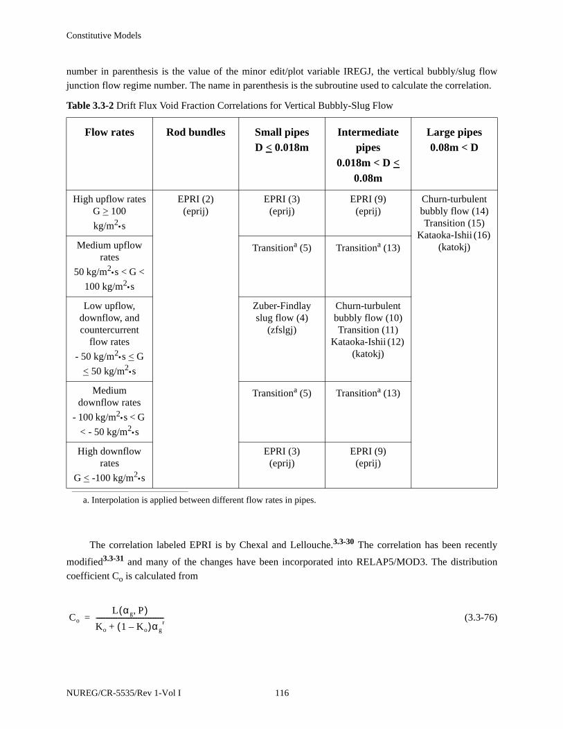
Constitutive Models
number in parenthesis is the value of the minor edit/plot variable IREGJ, the vertical bubbly/slug flow
junction flow regime number. The name in parenthesis is the subroutine used to calculate the correlation.
The correlation labeled EPRI is by Chexal and Lellouche.3.3-30 The correlation has been recently
modified3.3-31 and many of the changes have been incorporated into RELAP5/MOD3. The distribution
coefficient Co is calculated from
(3.3-76)
Table 3.3-2 Drift Flux Void Fraction Correlations for Vertical Bubbly-Slug Flow
Flow rates Rod bundles Small pipesD < 0.018m
Intermediate pipes
0.018m < D < 0.08m
Large pipes0.08m < D
High upflow ratesG > 100
kg/m2•s
EPRI (2)(eprij)
EPRI (3)(eprij)
EPRI (9)(eprij)
Churn-turbulentbubbly flow (14)Transition (15)
Kataoka-Ishii (16) (katokj)Medium upflow
rates
50 kg/m2•s < G <
100 kg/m2•s
Transitiona (5)
a. Interpolation is applied between different flow rates in pipes.
Transitiona (13)
Low upflow, downflow, and countercurrent
flow rates
- 50 kg/m2•s < G
< 50 kg/m2•s
Zuber-Findlayslug flow (4)
(zfslgj)
Churn-turbulentbubbly flow (10)Transition (11)
Kataoka-Ishii (12) (katokj)
Medium downflow rates
- 100 kg/m2•s < G
< - 50 kg/m2•s
Transitiona (5) Transitiona (13)
High downflow rates
G < -100 kg/m2•s
EPRI (3)(eprij)
EPRI (9)(eprij)
Co
L αg P,( )Ko 1 Ko–( )αg
r+----------------------------------------=
NUREG/CR-5535/Rev 1-Vol I 116
Constitutive Models
where
L(αg,P) = (3.3-77)
C1 = (3.3-78)
Pcrit = critical pressure
Ko = (3.3-79)
B1 = min (0.8, A1) (3.3-80)
A1 = (3.3-81)
Re = Reg if Reg > Ref or Reg < 0 (3.3-82)
= Ref otherwise (3.3-83)
Ref = local liquid superficial Reynolds number
= (3.3-84)
Reg = local vapor superficial Reynolds number
= (3.3-85)
r = (3.3-86)
The sign of jk is positive if phase k flows upwards and negative if it flows downwards. This
convention determines the sign of Reg, Ref, and Re.
The vapor drift velocity, vgj, for the Chexal-Lellouche correlation is calculated from
1 exp C1αg–( )–1 exp C1–( )–
---------------------------------------
4Pcrit2
P Pcrit P–( )---------------------------
B1 1 B1–( )ρg
ρf-----
1 4⁄
+
1
1 expRe
60 000,------------------
–+
----------------------------------------------
ρfjfDh
µf---------------
ρgjgDh
µg----------------
1 1.57ρg
ρf-----
+
1 B1–-------------------------------
117 NUREG/CR-5535/Rev 1-Vol I
Constitutive Models
(3.3-87)
where
C2 = 1 if C5 > 1 (3.3-88)
= if C5 < 1 (3.3-89)
C5 = (3.3-90)
C6 = (3.3-91)
C4 = 1 if C7 > 1 (3.3-92)
= if C7 < 1 (3.3-93)
C7 = (3.3-94)
D2 = 0.09144 m (normalizing diameter)
C8 = (3.3-95)
C9 = (1 - αg)B1 if Reg > 0 (3.3-96)
= min [0.7, (1 - αg)0.65] if Reg < 0 (3.3-97)
The parameter C3 depends on the directions of the vapor and liquid flows:
Upflow (both jg and jf are positive)
(3.3-98)
vgj 1.41ρf ρg–( )σg
ρf2
----------------------------1 4⁄
C2C3C4C9=
11 exp C6–( )–--------------------------------
150ρg
ρf-----
1 2⁄
C5
1 C5–---------------
11 exp C8–( )–--------------------------------
D2
D------
0.6
C7
1 C7–---------------
C3 max 0.50 2Ref
60000---------------–
exp,=
NUREG/CR-5535/Rev 1-Vol I 118
Constitutive Models
Downflow (both jg and jf are negative)
(3.3-99)
(3.3-100)
(3.3-101)
D1 = 0.0381 m (normalizing diameter) (3.3-102)
Countercurrent Flow (jg is positive, jf is negative)
(3.3-103)
(3.3-104)
(3.3-105)
D1 = 0.0381 (normalizing diameter) (3.3-106)
The parameters C2, C3, C4,..., C10 are from the Chexal-Lellouche correlation.3.3-30, 3.3-31
The correlation labeled Zuber-Findlay Slug Flow is by Zuber and Findlay.3.3-32,3.3-33 The
distribution parameter is given by
Co = 1.2 (3.3-107)
and the drift velocity is given by
C3
C10
2--------
2B
=
B21
1 0.05 Ref
35000---------------
0.4+
-------------------------------------------=
C10 2expRef
350000------------------
0.4
1.75 Ref0.03exp
Ref–50000---------------
D1
D------
2
–D1
D------
0.25
Ref0.001+=
C3
C10
2--------
2B
=
B21
1 0.05 Ref
35000---------------
0.4+
-------------------------------------------=
C10 2expRef
350000------------------
0.4
1.75 Ref0.03exp
Ref–50000---------------
D1
D------
2
–D1
D------
0.25
Ref0.001+=
119 NUREG/CR-5535/Rev 1-Vol I

Constitutive Models
(3.3-108)
The correlation labeled Kataoka-Ishii is by Kataoka and Ishii.3.3-34 The distribution parameter is
given by the modified Rouhani correlation3.3-35 used in TRAC-BF1,3.3-36
(3.3-109)
(3.3-110)
and the drift velocity is given by
for D* < 30 (3.3-111)
for D* > 30 (3.3-112)
where D* is the Bond number given by Equation (3.3-7) and the viscosity number, Nµf, is given by
(3.3-113)
The correlation labeled “churn turbulent bubbly flow” is by Zuber and Findlay.3.3-32,3.3-33 The
distribution parameter is given by the modified Rouhani correlation3.3-35 used in TRAC-BF1,3.3-36
Equation (3.3-109) and (3.3-110) and the drift velocity is given by
(3.3-114)
For intermediate pipes (for low upflow, downflow, and countercurrent flow rates) and large pipes (all
cases), the churn turbulent bubbly flow correlation is applied when
vgj 0.35ρf ρg–( )gD
ρf-----------------------------
1 2⁄=
Co C∞ C∞ 1–( )ρg
ρf-----
1 2⁄
–=
C∞ 1 0.2ρf gD( )1 2⁄
G 0.001+---------------------------
1 2⁄
+=
vgj 0.0019 D*( )0.809 ρg
ρf-----
0.157–
Nµf0.562– σg ρf ρg–( )
ρf2
----------------------------1 4⁄
=
vgj 0.030ρg
ρf-----
0.157–
Nµf0.562– σg ρf ρg–( )
ρf2
----------------------------1 4⁄
=
Nµf
µf
ρfσσ
g ρf ρg–( )------------------------
1 2⁄
1 2⁄-----------------------------------------------------------=
vgj 1.41σg ρf ρg–( )
ρf2
----------------------------1 4⁄
=
NUREG/CR-5535/Rev 1-Vol I 120

Constitutive Models
The Kataoka-Ishii correlation is applied when
(3.3-115)
where = 1.768. Linear interpolation is used between the two correlations.
Putney has also placed a countercurrent flow limitation (CCFL) on the drift flux parameters. The
limitation is based on the Kutateladze condition (see Section 3.4.7)
(3.3-116)
where
Kug = (3.3-117)
Kuf = (3.3-118)
m = 1 (3.3-119)
and Kucrit (using linear interpolation) is given by Table 3.3-3. This table for Kucrit as a function of D* is
from Wallis and Makkenchey.3.3-37 This has been used successfully in the RELAP-UK code.3.3-38 The
value of m = 1 was also used in the RELAP-UK code.
Table 3.3-3 Values of Kucrit for Kutateladze Condition
D* Kucrit
< 2 0
4 1.0
jg+ jg
σg ρf ρg–( )ρf
2----------------------------
14---
------------------------------------ jg1+≤ 0.5= =
jg+ ≥ jg2
+
jg2+
Kug1 2⁄ m Kuf
1 2⁄+ Kucrit1 2⁄=
α gvgρg
12---
σg ρf ρg–( )[ ]14---
-----------------------------------
α fvfρf
12---
σg ρf ρg–( )[ ]14---
-----------------------------------
121 NUREG/CR-5535/Rev 1-Vol I

Constitutive Models
On the flooding curve, the drift flux parameters satisfy the relationship
(3.3-120)
This flooding limit for vgj is applied for mass fluxes (G) larger than 100 kg/m2•s and for αg > 0.5.
Linear interpolation is used down to a mass flux of 50 kg/m2•s and to αg = 0.3, at which point the normal
drift flux correlations are used.
3.3.6.5 Slug Flow.
For vertical slug flow, the drift flux model is used. For non-vertical slug flow, the drag coefficient
model is used.
The drag coefficient model will first be discussed. Slug flow for non-vertical geometry is modeled as
a series of Taylor bubbles separated by liquid slugs containing small bubbles. A sketch of a slug flow
pattern is shown in Figure 3.3-5. The Taylor bubble has a diameter nearly equal to the pipe diameter and a
length varying from 1 to 100 pipe diameters.
Let αgs be the average void fraction in the liquid film and slug region. The void fraction of a single
Taylor bubble, αb, in the total mixture is then
(3.3-121)
10 2.1
14 2.5
20 2.8
28 3.0
> 50 3.2
Table 3.3-3 Values of Kucrit for Kutateladze Condition
D* Kucrit
vgj
1 αgCo–( )CoKucrit
ρf ρg–( )gσρf
2----------------------------
1 4⁄
αgCo
ρg
ρf-----
1 2⁄
m2 1 αgCo–( )+
----------------------------------------------------------------------------------------=
α b
αg αgs–1 α gs–-------------------=
NUREG/CR-5535/Rev 1-Vol I 122
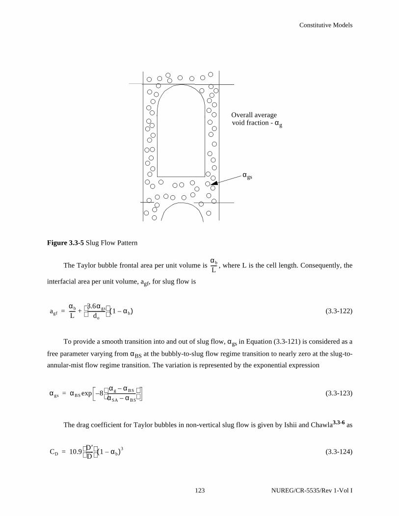
Constitutive Models
The Taylor bubble frontal area per unit volume is , where L is the cell length. Consequently, the
interfacial area per unit volume, agf, for slug flow is
(3.3-122)
To provide a smooth transition into and out of slug flow, αgs in Equation (3.3-121) is considered as a
free parameter varying from αBS at the bubbly-to-slug flow regime transition to nearly zero at the slug-to-
annular-mist flow regime transition. The variation is represented by the exponential expression
(3.3-123)
The drag coefficient for Taylor bubbles in non-vertical slug flow is given by Ishii and Chawla3.3-6 as
(3.3-124)
Figure 3.3-5 Slug Flow Pattern
Overall averagevoid fraction - αg
αgs
αb
L-----
agf
αb
L-----
3.6αgs
do---------------
1 αb–( )+=
αgs αBS 8α g αBS–αSA αBS–------------------------
–exp=
CD 10.9D ′D------
1 αb–( )3=
123 NUREG/CR-5535/Rev 1-Vol I
Constitutive Models
where D’ is the Taylor bubble diameter and αb is given by combining Equation (3.3-121) and Equation
(3.3-123).
The drag coefficient for small bubbles in non-vertical slug flow is given by Ishii and Chawla3.3-6 by
Equation (3.3-74).
For vertical slug flow, the interphase drag and shear terms are calculated using the same drift flux
correlations that are used in vertical bubbly flow.
3.3.6.6 Annular-Mist Flow.
Annular-mist flow is characterized by a liquid film along the wall and a vapor core containing
entrained liquid droplets. Let αff be the average liquid volume fraction of the liquid film along the wall.
Then, from simple geometric considerations, the interfacial area per unit volume can be shown to be
(3.3-125)
where Cann is a roughness parameter introduced to account for waves in the liquid wall film, αfd is the
average liquid volume fraction in the vapor core, for which
(3.3-126)
and do is the average diameter of the drops. For an annulus component, all the liquid is in the film and there
are no drops. Thus, αff = αf and αfd = 0 are used for an annulus. This was necessary to get downcomer
penetration following a cold leg break. This is discussed more in Volume IV.
A simple relation based on the flow regime transition criterion and liquid Reynolds number is used to
correlate the average liquid film volume fraction. For vertical flow regimes, the entrainment relation is
(3.3-127)
where uc is the critical entrainment superficial velocity given by the combination of Equation (3.3-13) and
(3.3-15).
For horizontal flow regimes, the entrainment relation is
agf
4Cann
D-------------
1 α ff–( )1 2⁄ 3.6α fd
do---------------
1 α ff–( )+=
α fd
α f α ff–1 α ff–------------------=
α ff α fCf 7.5 5–×10αgvg
uc-----------
6
–exp=
NUREG/CR-5535/Rev 1-Vol I 124

Constitutive Models
(3.3-128)
where vgL is the horizontal stratification critical velocity given by Equation (3.3-29). The term Cf is
expressed as
(3.3-129)
The interfacial friction factor, fi, for the liquid film takes the place of CD in Equation (3.3-68), and is
described by a standard correlation in the laminar region and is based on Wallis’ correlation in the
turbulent region.3.3-23 In the turbulent region, the Wallis correlation was modified to use the factor 0.02
rather than 0.005. This is the value used in RELAP5/MOD1,3.3-39 and it was selected because of the
MOD1 assessment. It is based on the vapor Reynolds number defined as
(3.3-130)
where
Dg = is the equivalent wetted diameter (3.3-131)
µg = viscosity of the vapor phase (3.3-132)
The values of fi are
fi = for Reg < 500
= ,
for 500 < Reg < 1500
= 0.02 {1 + 150 [1- (1 - αff)1/2]} for Reg > 1500 (3.3-133)
The interfacial drag coefficient CD for the drops is given by Ishii and Chawla3.3-6 from Equation
(3.3-74).
α ff α fCf 4.0 5–×10vg vf–
vgL------------------
6
–exp=
Cf 1.0 10 4– α fρf vfDµf----
0.25
–=
Reg
ρg vg vf– Dg
µg-------------------------------=
α g1 2⁄ D
64Reg---------
1500 Reg–1000
--------------------------- 64
Reg---------
Reg 500–1000
------------------------ 0.02 1 150 1 1 α ff–( )1 2⁄–[ ]+{ }+
125 NUREG/CR-5535/Rev 1-Vol I

Constitutive Models
3.3.6.7 Vertical Stratified Flow.
For the junction above the vertically stratified volume (junction j in Figure 3.3-6), the interphase
drag is based on the void fraction in the volume above (volume L). This is consistent with the junction-
based interphase drag. This is obtained as follows: The void fraction used in the junction j for the
junction-based interphase drag is given by
(3.3-134)
and is similar to Equation (3.3-34) except that αg,K is replaced by . This void fraction is given by
(3.3-135)
where strat takes on values from 0 to 1. For a vertically stratified volume, strat = 1, and
. For a non-vertically stratified volume, strat = 0, , and is given by Equation
(3.3-34). The smoothing parameter strat is given by
strat = strat1 • strat2 (3.3-136)
where
Figure 3.3-6 Three Vertical Volumes with the Middle Volume Being Vertically Stratified
α g j,*
I
L
j
j-1
K
αg j,* wj αg K,
* 1 wj–( ) α g L,•+•=
α g K,*
α g K,* strat αg L, 1 strat–( ) αg K,•+•=
αg K,* αg L,=
α g j,* αg L,= αg K,
* αg K,= αg j,*
NUREG/CR-5535/Rev 1-Vol I 126
Constitutive Models
(3.3-137)
(3.3-138)
Both strat1 and strat2 are limited to values between 0 and 1. Equation (3.3-137) for strat1 is a
modification of the approach used in RELAP5/MOD2. The variable strat1 exponentially turns off the
stratification effect when the volume above (volume L) becomes empty of liquid. When αf,L = 0.01, strat1
= 0.005. For strat2, the variables vm and vTb are the mixture velocity based on the volume centered
velocities and Taylor bubble rise velocity given by Equation (3.3-5).
A different method is used at junction j-1 below the vertically stratified volume. Equation (3.3-134),
(3.3-135), (3.3-136), and (3.3-138) are used, however, strat1 is given by
strat1 = 20 (αlevel - 0.05) (3.3-139)
where
αlevel = (3.3-140)
The variable αlevel is an implied non-dimensional mixture level position within volume K. The
coding is generalized to handle the case where the volumes and junctions are oriented downward. The
vertical stratification model is not intended to be a mixture level model, and a more mechanistic level
tracking model is described in Section 3.4.8.
If more than one junction is connected to the top, the volume above with the smallest void fraction
will be treated as the “above volume;” if more than one junction is connected to the bottom, the volume
below with the largest void fraction will be treated as the “below volume.”
3.3.6.8 Horizontal Stratified Flow.
By simple geometric consideration, one can show that the interfacial area per unit volume is
(3.3-141)
where Cst is a roughness parameter introduced to account for surface waves and is set to 1 at the present
time. (See Figure 3.1-2 for the definition of angle θ).
strat1 1 e0.5α f L,–
–=
strat2 2 1vm
vTb-------–
=
αg L, αg K,–α g L, αg I,–--------------------------
agf 4Cstθsin
πD-----------=
127 NUREG/CR-5535/Rev 1-Vol I
Constitutive Models
The interface Reynolds number is defined with the vapor properties and regarding liquid as the
continuous phase for which
(3.3-142)
where the equivalent wetted diameter, Di, for the interface is
(3.3-143)
The interfacial friction factor, fi, replaces CD in Equation (3.3-68) and is obtained by assuming
typical friction factor relationships for which
(3.3-144)
3.3.6.9 Inverted Flow Regimes.
These regimes arise when there is hot vapor in the cell and either hot walls or the reflood model is on.
The interphase drag relationships for post-CHF inverted flow regimes are treated in a similar fashion to the
corresponding pre-CHF flow regimes, except that the roles of vapor and liquid are interchanged.
3.3.6.9.1 Inverted Annular Flow
Immediately downstream of a quench front or CHF position, there may be an inverted annular flow
region if the combination of liquid flow and subcooling are high enough. The physical concept in the
model is the presence of vapor bubbles in the liquid core (just as there are liquid drops in the vapor core
region for annular-mist flow) and an annular gas layer between the walls and the core. The drag term [fgf in
Equation (3.3-68)] is the sum of the drag between the bubbles and the liquid in the core and the drag
between the vapor annulus and the outer surface of the core.
The drag coefficient for the bubbles is the Ishii-Chawla correlation given by Equation (3.3-74), and
the interfacial area is:
(3.3-145)
Rei
Diρg vg vf–µg
------------------------------=
Di
α gπDθ θsin+--------------------=
fi max
64Rei--------
0.3164
Rei0.25
----------------=
αgf
3.6αgb
do--------------- 1 αB–( )=
NUREG/CR-5535/Rev 1-Vol I 128
Constitutive Models
where:
αgb = the gas void fraction in the liquid core
do = the bubble diameter
αB = the fraction of the total area occupied by the steam annulus
The Weber number used to solve for the bubble diameter is 10. The annulus gas void fraction is an
exponential function of the total gas void fraction, similar to Equation (3.3-123), and is presented in
Volume IV of the RELAP5/MOD3 manuals. The core gas void fraction is:
(3.3-146)
where
Vcore = volume of the liquid core including bubbles
Vtot = volume of control volume
The annular shear force uses the Bharathan et al.3.3-40 equation for the drag coefficient:
CD = 4[0.005 + A(δ*)B] (3.3-147)
where
log10 A = (3.3-148)
B = (3.3-149)
δ* = (3.3-150)
The term δ* is the liquid wall film Deryagin number for which δ is the film thickness, and D* is the
dimensionless diameter Bond number given by Equation (3.3-7).
The interfacial area of the gas annular film per unit length in a pipe is
α gb
Vgas core,
Vcore-------------------
Vgas tot, Vgas ann,–Vtot Vgas ann,–
-----------------------------------------αg αB–1 αB–------------------= = =
0.56–9.07
D*----------+
1.634.74
D*----------+
δρf ρg–( )g
σ------------------------
1 2⁄
129 NUREG/CR-5535/Rev 1-Vol I
Constitutive Models
(3.3-151)
where
= inner diameter of annulus
D = diameter of pipe
(3.3-152)
where
Vcore = idealized volume of the gas core per unit length
Vtot = volume of control volume per unit length
Solving for the ratio from Equation (3.3-152) and putting it into Equation (3.3-151) yields:
(3.3-153)
3.3.6.9.2 Inverted Slug Flow
The inverted slug flow regime as envisioned by DeJarlais and Ishii3.3-41 consists of bubble-
impregnated liquid droplets (see Figure 3.3-7). The coded interfacial friction coefficients recognize the
liquid droplets, vapor blanket, and liquid slugs, but not the presence of bubbles in the slugs. Contributions
to the interfacial friction are recognized then, as coming from two sources: (a) the liquid droplet interfaces
in the vapor annulus and (b) the liquid slug/annulus interface. It is assumed that the liquid slugs are so long
that any contributions to interfacial friction at their ends are negligible.
The interfacial areas for the annulus/droplet portion and the slug/annulus portion are derived
analogously to those for nonvertical slug flow (Section 3.3.6.5). The void fraction of the liquid slug, αB, is
analogous to that for a Taylor bubble, αTb, and the average droplet void in the vapor blanket, αdrp, is
analogous to the average void, αgs, in the liquid annulus for slug flow. That is, the interfacial areas are
computed for inverted slug flow by simply reversing the liquid and vapor phases from slug flow. The
agf ann,πD ′π4---D2----------
4D ′D2
---------= =
D ′
Vcore
Vtot------------
π4---
π4------
D ′ 2
D2--------
D ′ 2
D2-------- 1 αB–= = =
D ′D------
agf ann,4D---- 1 αB–( )1 2⁄=
NUREG/CR-5535/Rev 1-Vol I 130

Constitutive Models
droplet void, αdrp, in the vapor annulus is an expression that exponentially increases the portion of αf due
to droplets as αg increases until the transition void, αSA, is reached, at which point all of the liquid is
appropriately assumed to be in droplet form. The value for the Weber number used is 12.0.
The drag coefficients for the annulus/droplet portion and the slug/annulus portion are analogous to
those for non-vertical slug flow, except that the liquid and vapor phases are reversed.
3.3.6.9.3 Mist Flow
The mist flow regime is discussed in Section 3.3.6.4, Dispersed Flow. For mist pre-CHF, We = 3.0
and ; for mist and mist post-CHF, We = 12.0 and µm = µg.
3.3.7 Coefficient of Virtual Mass
The coefficient of virtual mass is determined based on the junction flow regime map. The calculation
of the drag due to the virtual mass effect (dynamic drag) is based on an objective and symmetric
formulation of the relative acceleration.3.3-42 The inertial drag force per unit volume in the phasic
momentum equations is written as
(3.3-154)
where
Figure 3.3-7 Flow Regimes Before and After the Critical Heat Flux (CHF) Transition
Bubbly
Inverted slug Dispersed dropletInverted annular
Annular or annular-mist
CHF CHF
Slug
µm
µg
α g( )2.5---------------=
FAgf Cαg 1 αg–( )ρ ∂∂t---- vg vf–( )–=
131 NUREG/CR-5535/Rev 1-Vol I
Constitutive Models
ρ = αgρg + (1 - αg)ρf (3.3-155)
FAgf = force per unit volume due to dynamic drag
The factor, Cαg(1 - αg)ρ, is chosen to ensure a smooth transition between αg = 0 and αg = 1.0. This
factor also gives the proper limit, Cαgρf in the thinly dispersed bubbly flow, and C(1 - αg)ρg in the
dispersed droplet flow. The virtual mass coefficient, C, is given3.3-43 as
for 0 < αg < 1/2 (3.3-156)
for 1/2 < αg < 1 (3.3-157)
It may be appropriate to assume that C = 0 should be used for separated or stratified flow. At present,
the value of C defined by Equation (3.3-156) and (3.3-157) is used without regard to the flow regime.
3.3.8 Wall Friction
The wall friction is determined based on the volume flow regime map. The wall friction force terms
include only wall shear effects. Losses due to abrupt area change are calculated using mechanistic form-
loss models. Other losses due to elbows or complicated flow passage geometry are modeled using energy-
loss coefficients that must be input by the user.
Emphasis was placed on obtaining reasonable values for wall friction in all flow regimes in the
development of the wall friction model. The flow regime models are discussed in Section 3.3.1 through
Section 3.3.4.
The wall friction model is based on a two-phase multiplier approach in which the two-phase
multiplier is calculated from the Heat Transfer and Fluid Flow Service (HTFS)-modified Baroczy
correlation.3.3-44 The individual phasic wall friction components are calculated by apportioning the two-
phase friction between the phases using a technique derived by Chisholm3.3-45 from the Lockhart-
Martinelli3.3-46 model. The partitioning model is based on the assumption that the frictional pressure drop
may be calculated using a quasi-steady form of the momentum equation.
3.3.8.1 The Two-Phase Friction Multiplier Approach.
The Lockhart-Martinelli model computes the overall friction pressure drop in terms of the liquid-
alone wall friction pressure drop
C12---
1 2αg+( )1 αg–( )
-----------------------=
C12---
3 2α g–( )αg
-----------------------=
NUREG/CR-5535/Rev 1-Vol I 132

Constitutive Models
(3.3-158)
or the vapor-alone wall friction pressure drop
(3.3-159)
where φf and φg are the liquid-alone and vapor-alone two-phase Darcy-Weisbach friction multipliers,
respectively. The phasic wall friction pressure gradients are expressed as
(3.3-160)
for the liquid alone, and
(3.3-161)
for the vapor alone, where the prime indicates the liquid and vapor-alone Darcy-Weisbach friction factors,
respectively, calculated at the respective Reynolds numbers
(3.3-162)
and
(3.3-163)
The liquid and vapor mass flow rates, respectively, are defined as
Mf = αfρfvfA (3.3-164)
and
xddP
2φφf
2
xddP
f=
xddP
2φφg
2
xddP
g=
xddP
f
λ f′ Ref ′( )Mf
2
2DρfA2
----------------------------=
xddP
g
λg′ Reg′( )Mg
2
2DρgA2-----------------------------=
Ref′ MfD
µfA-----------=
Reg′ MgD
µgA------------=
133 NUREG/CR-5535/Rev 1-Vol I
Constitutive Models
Mg = αgρgvgA (3.3-165)
Throughout the current literature, the overall two-phase friction pressure gradient is calculated using
two-phase friction multiplier correlations. However, regardless of the correlation used, the multipliers may
be interrelated using Equation (3.3-158) through Equation (3.3-161) and the Lockhart-Martinelli3.3-46 ratio
defined as
(3.3-166)
3.3.8.2 The HTFS Two-Phase Friction Multiplier Correlation.
The HTFS correlation3.3-44 is used to calculate the two-phase friction multipliers. This correlation
was chosen because it is correlated to empirical data over very broad ranges of phasic volume fractions,
phasic flow rates and phasic flow regimes. The correlation has also been shown to give good agreement
with empirical data.
The HTFS correlation for the two-phase friction multiplier3.3-44 is expressed as
(3.3-167)
for the liquid-alone multiplier, or
(3.3-168)
for the vapor-alone multiplier, where C is the correlation coefficient and is the Lockhart-Martinelli ratio
given by Equation (3.3-166). The correlation term is expressed in terms of scalar mass flux, G, and the
Baroczy dimensionless property index, Λ, such that
2 < C = -2 + f1 (G) T1 (Λ, G) (3.3-169)
where
f1 (G) = 28 - 0.3 (3.3-170)
χ2
dPdx------
f
dPdx------
g
--------------φg
2
φf2
-----= =
φf2 1
Cχ----
1
χ2-----+ +=
φg2 χ2 Cχ 1+ +=
χ
G
NUREG/CR-5535/Rev 1-Vol I 134
Constitutive Models
T1 (Λ, G) = (3.3-171)
Λ = (3.3-172)
The terms ρ, µ, α and v denote the density, viscosity, volume fraction and velocity, respectively.
If the HTFS correlation is combined with the wall friction formulations by combining Equation (3.3-
158) through (3.3-161), Equation (3.3-164) through (3.3-166), Equation (3.3-168), and (3.3-169), then
(3.3-173)
3.3.8.3 Partitioning of Wall Friction.
Two-phase friction can be modeled in terms of two-phase friction multipliers and known friction
factors using the method developed by Lockhart-Martinelli.3.3-46 Chisholm3.3-45 also developed a
theoretical basis for the Lockhart-Martinelli model that provides a rationale for partitioning the overall
wall friction between the phases which is independent of the model for interfacial friction.
From the theoretical basis developed by Chisholm, the phasic momentum equations can be expressed
in scalar form as
(3.3-174)
for the liquid, and
(3.3-175)
for the vapor, where τf and τg are the liquid and vapor wall shear stresses, respectively, pf and pg are the
liquid and vapor wetted perimeters, respectively, and SFI is a stress gradient due to interphase friction.
Eliminating the overall pressure gradient between these two equations determines the interfacial friction
term in terms of the ratio of the phasic shear stresses and phasic wetted perimeters.
explog10Λ 2.5+( )2
2.4 G 10 4–( )–-------------------------------------–
ρg
ρf-----
µf
µg-----
0.2
dPdx------
2φ
φf2 dP
dx------
f
φg2 dP
dx------
g
12D------- λ{ f
′ ρf α fvf( )2 C λ f′ ρf α fvf( )2λg
′ ρg αgvg( )2[ ] 1 2⁄+= = =
λg′ ρg α gvg( )2 }+
α fA xddP
2φτ fpf– SFI+ 0=
α gAxd
dP
2φτgpg– SFI– 0=
135 NUREG/CR-5535/Rev 1-Vol I
Constitutive Models
(3.3-176)
where the interphase friction term, SR, is defined as
(3.3-177)
Equation (3.3-176) can be rearranged to give a relation for the interfacial shear stress gradient in
terms of the ratio of the phasic wall shear forces. This relation can then be substituted into the quasi-static
momentum balances to give a relation for the individual phasic wall shear force gradients in terms of the
overall wall friction and the ratio of the phasic wall shear stresses.
(3.3-178)
and
(3.3-179)
These relations are nothing more than a rearrangement of the quasi-static momentum equations and
have only eliminated one unknown, the interfacial shear stress in terms of another unknown, Z2, the ratio
of the phasic wall friction gradients. Chisholm postulated that the phasic wall shear stress could be
determined using Darcy-Weisbach friction factors computed from Reynolds numbers based on phasic
properties as
(3.3-180)
where
λ(Ref) = liquid Darcy friction factor (3.3-181)
Ref = liquid Reynolds number (3.3-182)
1 SR
αg
α f-----
+
1 SR–( )---------------------------
τ fpf
α f--------
τgpg
α g----------
--------------- Z2= =
SR
SFI
αgAxd
dP
2φ
---------------------------=
τ fpf α f xddP
2φ
Z2
α g α fZ2+
-----------------------
=
τgpg αg xddP
2φ
1
αg α fZ2+
----------------------- =
τ f λ Ref( )ρfvf
2
2----------=
NUREG/CR-5535/Rev 1-Vol I 136
Constitutive Models
= (3.3-183)
Df = liquid hydraulic diameter (3.3-184)
= (3.3-185)
Af = liquid flow area (3.3-186)
= αfA (3.3-187)
pf = liquid wetted perimeter (3.3-188)
= αfwp (3.3-189)
where αfw is the liquid fraction on the wall, and the vapor shear stress is defined in an analogous manner
based on vapor properties. Substituting the liquid shear stress from Equation (3.3-180) and the liquid
wetted perimeter from Equation (3.3-189) and the analogous expressions for the vapor friction factor and
wetted perimeter, defines the unknown parameter Z2
(3.3-190)
Substituting Equation (3.3-190) into the relations for the phasic wall friction forces Equation (3.3-
178) and (3.3-179) yields equations which determine the magnitude of the phasic wall friction force in
terms of the overall wall friction force and the ratio of the phasic wall frictional forces, independent of the
formulation for the interfacial shear forces and independent of the particular model for the overall wall
frictional force.
It should be noted that the calculation of the phasic friction factors using the Reynolds numbers
defined above and the assumption that two-phase flows behave similarly to single-phase flows in the
laminar, transition, and turbulent regimes provides the rationale relating Equation (3.3-178) and (3.3-179)
to empirical data. It is this same rationale that allows the correlating term Z2 to be expressed in terms of
friction factors that are independent of interphase friction as given by Equation (3.3-176). It is this equation
that forms the basis for apportioning the overall two-phase wall friction between the phases.
ρfvfDf
µf---------------
4Af
pf---------
Z2λ f Ref( )ρfvf
2α fw
α f--------
λg Reg( )ρgvg2αgw
αg--------
----------------------------------------=
137 NUREG/CR-5535/Rev 1-Vol I

Constitutive Models
3.3.8.4 RELAP5 Wall Friction Coefficients.
The RELAP5 phasic momentum equations, Equation (3.1-6) and (3.1-7) can be written in a quasi-
static form similar to Equation (3.3-174) and (3.3-175), except that the wall friction terms are in terms of
the RELAP5 wall friction coefficients instead of phasic wall shear stresses. Comparison of these two forms
of the momentum equations provides a definition of the RELAP5 phasic wall friction coefficients as
(3.3-191)
and
(3.3-192)
Taking the sum of these two equations gives the overall quasi-static, two-phase wall friction pressure
gradient as
(3.3-193)
3.3.8.5 Flow Regime Factors for Phasic Wall Friction.
Phasic wall friction is expressed in terms of wall shear stress, which, in turn, requires knowledge of
the surface area wetted by each phase. From the flow regime model discussed in Section 3.3.1 through
Section 3.3.4 expressions for the wall film phasic volume fractions can be derived. Using these
expressions, the phasic wall friction factor that appears in Equation (3.3-180) may then be computed.
In the flow regime map, eight flow regimes are modeled, which are: for pre-CHF heat transfer, the
bubbly, slug, and annular-mist; for post-CHF heat transfer, the inverted-annular, inverted-slug and mist;
and for stratified flow, the vertically and horizontally stratified. For the transition regime between pre- and
post-CHF heat transfer, an interpolation scheme is also implemented in the code.
To implement flow regime effects in the two-phase wall friction model, first consider the wall liquid
and vapor volume fractions. These terms are
(3.3-194)
FWF α fρfvf( )A τ fpf α f xddP
2φ
Z2
α g α fZ2+
-----------------------
A= =
FWG α gρgvg( )A τgpg α g xddP
2φ
1
αg α fZ2+
----------------------- A= =
FWF αgρfvf( )A FWG α gρgvg( )A+xd
dP
2φ
A=
pf
p---- α fw=
NUREG/CR-5535/Rev 1-Vol I 138

Constitutive Models
which represents the liquid volume fraction in the wall film, and
(3.3-195)
which represents the vapor volume fraction in the wall film, where the terms pf, pg, and p are the
perimeters wetted by the liquid, vapor, and mixture, respectively. Then, from the flow regime model, these
are formulated for all of the flow regimes as follows:
For the bubbly regime,
αfw = αf and αgw = αg (3.3-196)
where αf, αg are the overall liquid and vapor volume fractions, respectively.
For the slug regime,
αfw = 1 - αgs and αgw = αgs (3.3-197)
where αgs is given by Equation (3.3-123).
For the annular-mist regime,
αfw = (αff)1/4 and αgw = 1 - (αff)
1/4 (3.3-198)
where αff is given by Equation (3.3-128).
For the inverted-annular regime,
αfw = 1 - (αgg)1/4 and αgw = (αgg)1/4 (3.3-199)
where αgg is the inverted form of Equation (3.3-128).
For the inverted-slug regime,
αfw = αfs and αgw = 1 - αfs (3.3-200)
pg
p----- α gw=
139 NUREG/CR-5535/Rev 1-Vol I
Constitutive Models
where αfs is the inverted form of Equation (3.3-123).
For the mist regime,
αfw = αf and αgw = αg (3.3-201)
similar to the bubbly regime.
For the vertically stratified regime,
αfw = αf and αgw = αg (3.3-202)
For the horizontally stratified regime,
(3.3-203)
where θ results from the solution of Equation (3.1-60).
3.3.8.6 The Friction Factor Model.
In RELAP5 the Darcy-Weisbach friction factor is computed from correlations for laminar and
turbulent flows with interpolation in the transition regime.There are two turbulent flow friction factor
models. The first model computes the turbulent friction factor using an engineering approximation to the
Colebrook-White correlation,3.3-47 while the second model uses an exponential function with users’ input
coefficients.
The friction factor model is simply an interpolation scheme linking the laminar, laminar-turbulent
transition, and turbulent flow regimes. The laminar friction factor is calculated as
(3.3-204)
where Re is the Reynolds number and ΦS is a user-input shape factor for noncircular flow channels. The
friction factor in the transition region between laminar and turbulent flows is computed by reciprocal
interpolation as
for 2200 < Re < 3000 (3.3-205)
α fw 1θπ--- and α gw–
θπ---= =
λL64
ReΦS-------------- 0 Re 2200≤ ≤,=
λL T, 3.758250Re
------------– λT 3000, λL 2200,–( ) λL 2200,+=
NUREG/CR-5535/Rev 1-Vol I 140
Constitutive Models
where λL,2200 is the laminar factor at a Reynolds number of 2200, λT,3000 is the turbulent friction factor at
a Reynolds number of 3000, and the interpolation factor is defined to lie between zero and one.
The turbulent friction factor is given by the Zigrang-Sylvester approximation3.3-48 to the Colebrook-
White correlation3.3-47 as,
(3.3-206)
where ε is the surface roughness, and the other variables have been defined previously. The Zigrang-
Sylvester equation, Equation (3.3-206), has the advantage that it is an explicit relation for the friction
factor, while the Colebrook-White correlation is a transcendental function requiring iteration for the
determination of the friction factor. Reference 3.3-48 incorrectly uses 1.114 rather than the correct value
1.14.
3.3.8.7 Heated Wall Effect.
The friction model as described above applies to unheated surfaces. The user may correct the
isothermal friction factor for the variation of the fluid viscosity near a heated surface using the relationship
used in the VIPRE code.3.3-49 This relation is given by
(3.3-207)
where fiso is the friction factor evaluated with properties at the bulk fluid temperature, PH is the heated
perimeter of the surface, PW is the wetter perimeter of the surface, µwall is the viscosity evaluated at the
surface temperature, µbulk is the viscosity evaluated at the bulk fluid temperature, and the exponent D is a
user-input constant (viscosity ratio exponent). The default value in the code for the viscosity ratio exponent
D is 0, which results in no viscosity variation effect on wall friction. Rosenhow and Hartnett3.3-50 indicate
a range of values for tubes from the literature for the exponent D. The values are 0.50 to 0.58 for liquid
laminar flow, -0.012 to 0.25 for liquid turbulent flow, 0.8 to 1.35 for gas laminar flow, and -0.1 for gas
turbulent flow.
3.3.9 Wall Heat Transfer Models
In RELAP5/MOD3.2 the total wall heat flux (q”) is the heat flux to the vapor plus the heat flux to the
liquid
1
λT
---------- 2log10ε
3.7D------------
2.51Re
---------- 1.14 2log10εD----
21.25
Re0.9-------------–
–+
–=
ffiso------- 1
PH
PW-------
µwall
µbulk-----------
D
1–+=
141 NUREG/CR-5535/Rev 1-Vol I
Constitutive Models
q" = hg (Tw - Trefg) + hf (Tw - Treff) (3.3-208)
where
hg = heat transfer coefficient to gas
hf = heat transfer coefficient to liquid
Tw = wall temperature
Trefg = gas reference temperature
Treff = liquid reference temperature
The reference temperatures can be the local gas or liquid temperature or the saturation temperature,
depending on the heat transfer coefficient correlation being used.
A code user may flag a heat transfer structure as a reflood structure. Structures flagged as reflood
structures employ axial conduction. RELAP5/MOD3.2 uses the same wall heat transfer logic for reflood
flagged surfaces as it does for other surfaces.
A boiling curve is used in RELAP5 to govern the selection of the wall heat transfer correlations when
the wall surface temperature is above the saturation temperature (superheated relative to the saturation
temperature based on total pressure). When a hydraulic volume is voided and the adjacent surface
temperature is subcooled, steam condensation on the surface is predicted. If noncondensable gases are
present, the phenomena is more complex because while boiling is a function of the wall superheat based on
the total pressure, condensation is based on the partial pressure of steam. When the wall temperature is less
than the saturation temperature based on total pressure, but greater than the saturation temperature based
on steam partial pressure, a convection condition exists. Figure 3.3-8 illustrates these three regions.
There are many factors to consider when deciding which convective heat transfer coefficient
correlation to use. Relative factors that are addressed by the MOD3.2 logic are: (a) is the pressure above
the critical pressure, (b) is the wall temperature above the saturation temperature, (c) is a noncondensable
gas present, (d) is the fluid liquid, two-phase, or vapor, (e) is the heat flux above the critical heat flux
(CHF), and (f) is the film boiling heat flux greater than the transition boiling heat flux? The decision logic
in RELAP5 leads to the selection of the appropriate correlation for the heat transfer coefficient that is used
to find the heat flux.
The heat transfer mode number is a code output parameter used to inform users of the heat transfer
regime or correlation selected by the code. Twelve mode numbers from 0 to 11 are possible, as shown in
Figure 3.3-9, where
NUREG/CR-5535/Rev 1-Vol I 142
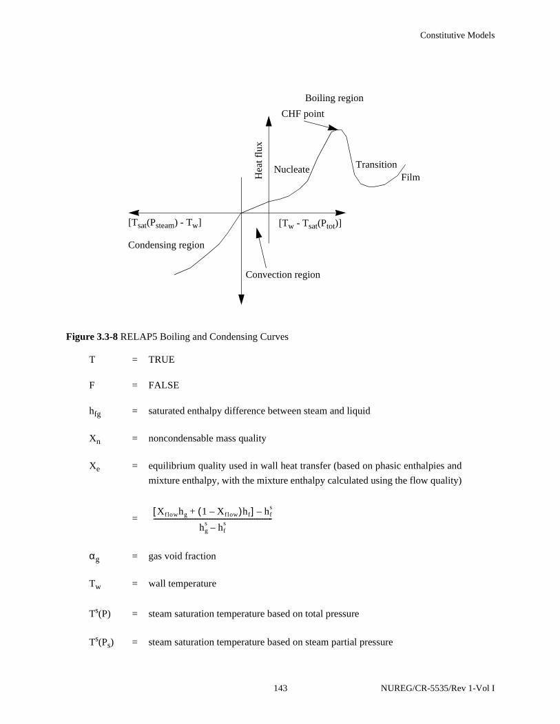
Constitutive Models
T = TRUE
F = FALSE
hfg = saturated enthalpy difference between steam and liquid
Xn = noncondensable mass quality
Xe = equilibrium quality used in wall heat transfer (based on phasic enthalpies and
mixture enthalpy, with the mixture enthalpy calculated using the flow quality)
=
αg = gas void fraction
Tw = wall temperature
Ts(P) = steam saturation temperature based on total pressure
Ts(Ps) = steam saturation temperature based on steam partial pressure
Figure 3.3-8 RELAP5 Boiling and Condensing Curves
Convection region
Hea
t flu
x
[Tsat(Psteam) - Tw]
Condensing region
[Tw - Tsat(Ptot)]
FilmTransition
CHF point
Boiling region
Nucleate
Xflowhg 1 Xflow–( )hf+[ ] hfs–
hgs hf
s–-----------------------------------------------------------------------
143 NUREG/CR-5535/Rev 1-Vol I
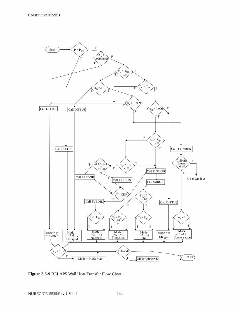
Constitutive Models
Figure 3.3-9 RELAP5 Wall Heat Transfer Flow Chart
Start
.99999999TXn > F
T
F
Call PREBUN
αg > 0.999T
Xn > 0.999
Call DITTUS
Call DITTUS
T
q”FB>
αg = 1
FT F
q” < CHF
Tf < Tspt
Xn < 1.E-9
Mode = Mode + 20
Reflood?
Mode=Mode+40 Return
FT
F
T
Tf < Tspt
T
Tf < Tspt
F F T
Call SUBOIL
Call PREDNB
q”TB
Call SUBOIL
Tw > Tspt+100
Call PSTDNB
Tw > Tspt+600
F
T
F
TF
T
Call DITTUSF
T
Tw < Tspt
Tw< Tspp
F
F
T F
T
Call DITTUS
T
F
-.001
Call CONDEN
Colburn-Hougenfailed
P > Pcrit
αg <.1
Mode = 0,Air-water
Mode1 =P>Pcrit2 = liquid
Mode = 9
1Φ, gas
Mode=10 =11
Condensation
T
F
Go to Mode 2F
Mode=3 =4Nucleate
Mode=5 =6
Transition
Mode=7 =8Film
T
-.05
T
Geo < 134
>150or
F
NUREG/CR-5535/Rev 1-Vol I 144
Constitutive Models
Tf = liquid temperature
CHF = critical heat flux
q" = heat flux
q"FB = film boiling heat flux
q"TB = transition boiling heat flux
Geom = type of hydraulic cell
1Φ = single-phase
If a noncondensable gas is present, 20 is added to the mode number; and another 40 is added if the
surface is a reflood surface. Most of this logic is built into the HTRC1 subroutine. The heat transfer
coefficients are determined in one of five subroutines: DITTUS, PREDNB, PREBUN, PSTDNB, and
CONDEN. Subroutine CONDEN calculates the coefficients when the wall temperature is below the
saturation temperature based on the partial pressure of steam. DITTUS is called for single-phase liquid or
vapor conditions. PREDNB contains the nucleate boiling correlations for all surfaces except horizontal
bundles and PREBUN is used for the outer surface of horizontal bundles of rods or tubes. PSTDNB has the
transition and film boiling correlations. Subroutine CHFCAL determines the critical heat flux for all
surfaces using a table lookup method. If reflood is on, CHFCAL has been called prior to the call to
HTRC1. Subroutine SUBOIL calculates the vapor generation rate in the superheated liquid next to a
superheated wall.
RELAP5 wall heat transfer correlations are based mainly on internal flow in pipes. Additional
geometries considered in the logic are vertical parallel plates, vertical and horizontal tube bundles and
horizontal flat plates.
3.3.10 Wall Heat Transfer Correlations
The boiling curve uses the Chen3.3-51 boiling correlation up to the critical heat flux point. A table
lookup method3.3-52 developed by Groeneveld, Cheng, and Doan is used for the prediction of the critical
heat flux. Code users also have the option of using a critical heat flux correlation developed by the Czech
Republic.3.3-53 When the wall superheat exceeds the critical value, the heat flux for both the transition
boiling and the film boiling regimes are calculated and the maximum value is used. This eliminates the
need for a prediction of a minimum film boiling temperature. The Chen-Sundaram-Ozkaynak
correlation3.3-54 is used for transition boiling and a modified Bromley correlation3.3-55 is used for film
boiling.
145 NUREG/CR-5535/Rev 1-Vol I
Constitutive Models
To obtain the fraction of the boiling heat flux which causes steam generation near a superheated wall,
the Lahey method3.3-56 is used. The expression for the mass transfer rate per unit volume near a wall, Γw,
is
(3.3-209)
where
q" = total wall heat flux
Aw = wall surface area
V = cell volume
Mul = multiplier
The multiplier is defined as
(3.3-210)
where
hcr = critical enthalpy for net voids calculated using the Saha-Zuber3.3-57
correlation (see Volume IV)
ε = the pumping term
= (3.3-211)
Using this multiplier as computed in Equation (3.3-210) resulted in time-step-to-time-step void
fraction oscillations in a heated vertical tube calculation. The oscillations could be suppressed by taking a
very small time step. However, the required time step was a factor of 100 times smaller than the time step
set by the Courant limit. In addition, in some cases, the average of the void fraction in the oscillatory case
was not the same value as the void fraction in the non-oscillatory case. The root cause was traced to very
large changes in the multiplier from time step to time step as a result of the large changes in the saturation
enthalpy because of large changes in the pressure that resulted from the large changes in the void fraction.
Consequently, the algebraic equation for the multiplier was replaced by a first-order relaxation differential
Γw
q″Aw
V hg′ hf
′–( )-------------------------Mul=
Mulhf hcr–
hfs hcr–( ) 1 ε+( )
---------------------------------------=
ρf hfs min hf hf
s,( )–[ ]ρghfg
------------------------------------------------
NUREG/CR-5535/Rev 1-Vol I 146

Constitutive Models
model that used a relaxation time constant of 100 ms. The algebraic equation is the same as the relaxation
model in the limit as the time constant goes to zero. Use of this relaxation model resulted in non-oscillatory
void fractions for all time step sizes up to the Courant limit. Use of a smaller time constant of 20 ms did not
suppress the oscillations; while use of a 50 ms time constant resulted in suppressing the oscillation in most
of the cases, but not all of them.
The finite difference equation for the multiplier that will be used in the subcooled boiling model that
corresponds to this first-order relaxation equation is
(3.3-212)
where
= this is the multiplier that is used for the time step
= this is the multiplier that was used in the previous time step
= this is the multiplier that was computed in Equation (3.3-210)
= relaxation time constant (100 ms was used)
Notice, that as the time step goes to zero, the multiplier that is used is equal to the previous time step
value, and as the time step gets very large, the multiplier that is used is equal to the value computed in
Equation (3.3-210). For a time step equal to the relaxation time, the multiplier that is used is equal to the
average of the previous multiplier and the value computed by Equation (3.3-210).
Convection mode calculations rely on evaluating forced convection, laminar convection, and natural
convection and selecting the maximum of these three. The correlations are by Dittus-Boelter,3.3-58
Kays,3.3-59 and Churchill-Chu,3.3-60 respectively.
For parallel plates the Petukhov correlation3.3-61 is used in place of the Dittus-Boelter correlation,
and the Elenbaas3.3-62 correlation is used instead of the Churchill-Chu correlation.
RELAP5 treats vertical bundles differently than pipes. The turbulent convection coefficient is
multiplied by the tube pitch-to-diameter ratio as suggested by Inayatov.3.3-63
Horizontal bundles in RELAP5 differ from pipes in their nucleate boiling, critical heat flux, and
natural convection prediction methods. Nucleate boiling predictions follow the Polley-Ralston-Grant
Mulused Mulprevious ∆t( ) τ⁄[ ] Mulcomputed+1 ∆t( ) τ⁄[ ]+
-----------------------------------------------------------------------------------=
Mulused
Mulprevious
Mulcomputed
τ
147 NUREG/CR-5535/Rev 1-Vol I
Constitutive Models
method3.3-64 and prediction of critical heat flux uses the Folkin-Goldberg method.3.3-65 Horizontal bundles
use the Churchill-Chu3.3-66 horizontal cylinder correlation.
There are two methods available to the user for calculating the heat transfer coefficients in the
condensation mode for all geometries. The default method uses the maximum of Nusselt3.3-67 and
Shah.3.3-68 When noncondensable gases are present, the default method uses the Colburn-Hougen3.3-69
iteration method to solve for the interface temperature between the steam and liquid and uses this value in
the heat flux calculation. The alternate method uses Nusselt’s3.3-67 laminar film coefficient modified for
gas turbulence and noncondensable gases using the multipliers developed by Vierow and Schrock.3.3-70
RELAP5 has a reflood heat transfer model developed by the Paul Scherrer Institute in
Switzerland.3.3-71
Details of heat transfer coefficient correlations and implementation are given in Volume IV.
3.3.11 Interphase Mass Transfer
The interphase mass transfer is modeled according to the volume flow regime discussed in Section
3.3.1 through Section 3.3.4. It is used to determine the phasic interfacial area and to select the interphase
heat transfer correlation for superheated liquid (SHL), subcooled liquid (SCL), superheated gas (SHG),
and subcooled gas (SCG).
The mass transfer model is formulated so that the net interfacial mass transfer rate is composed of
two components; the mass transfer rate in the bulk fluid, and the mass transfer rate near the wall. It is
expressed as
Γg = Γig + Γw (3.3-213)
where Γig is given by Equation (3.1-49) and Γw is discussed briefly in Section 3.3.10 and is presented in
more detail in Volume IV.
For components not modeling wall heat transfer and for the general bulk mass transfer processes, the
interfacial mass transfer model in the bulk fluid depends on the volume flow regime. In the bubbly flow
regime for a condition of superheated liquid, interfacial mass transfer is the larger of either the model for
bubble growth developed by Plesset and Zwick3.3-72 or the model for convective heat transfer for a
spherical bubble (modified Lee and Ryley).3.3-73 For the bubbly flow regime with a condition of
superheated vapor, an interphase heat transfer coefficient is assumed that is high enough that the vapor
temperature will relax toward the equilibrium (saturation) condition. Analogously, in the mist flow regime
for the condition of superheated vapor, a convective heat transfer model for a spherical droplet3.3-73 is used
for the interphase heat transfer coefficient. For mist flow with superheated liquid, an interphase heat
NUREG/CR-5535/Rev 1-Vol I 148
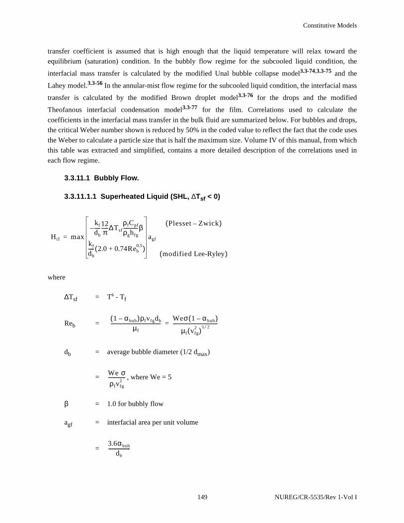
Constitutive Models
transfer coefficient is assumed that is high enough that the liquid temperature will relax toward the
equilibrium (saturation) condition. In the bubbly flow regime for the subcooled liquid condition, the
interfacial mass transfer is calculated by the modified Unal bubble collapse model3.3-74,3.3-75 and the
Lahey model.3.3-56 In the annular-mist flow regime for the subcooled liquid condition, the interfacial mass
transfer is calculated by the modified Brown droplet model3.3-76 for the drops and the modified
Theofanous interfacial condensation model3.3-77 for the film. Correlations used to calculate the
coefficients in the interfacial mass transfer in the bulk fluid are summarized below. For bubbles and drops,
the critical Weber number shown is reduced by 50% in the coded value to reflect the fact that the code uses
the Weber to calculate a particle size that is half the maximum size. Volume IV of this manual, from which
this table was extracted and simplified, contains a more detailed description of the correlations used in
each flow regime.
3.3.11.1 Bubbly Flow.
3.3.11.1.1 Superheated Liquid (SHL, ∆Tsf < 0)
where
∆Tsf = Ts - Tf
Reb =
db = average bubble diameter (1/2 dmax)
= , where We = 5
β = 1.0 for bubbly flow
agf = interfacial area per unit volume
=
Hif max
kf
db-----
12π------∆Tsf
ρfCpf
ρghfg------------β–
kf
db----- 2.0 0.74Reb
0.5+( )
agf
Plesset Zwick–( )
modified Lee-Ryley( )
=
1 αbub–( )ρfvfgdb
µf-----------------------------------------
Weσ 1 αbub–( )
µf vfg2( )1 2⁄-------------------------------------=
We σρfvfg
2--------------
3.6αbub
db------------------
149 NUREG/CR-5535/Rev 1-Vol I

Constitutive Models
αbub = max (αg, 10-5)
vfg = vg - vf
3.3.11.1.2 Subcooled Liquid (SCL, ∆Tsf > 0)
= 0.0 αg = 0.0
where
F5 = 0.075 αbub > 0.25
= 1.8φC exp(-45αbub) + 0.075 αbub < 0.25
C = 65.0 - 5.69 x 10⁻⁵ (P - 1.0 x 10⁵) P < 1.1272x10⁶ Pa
= P > 1.1272x10⁶ Pa
P = pressure (Pa)
φ = 1.0 |vf| < 0.61 m/s
= [1.639344|vf|]0.47 |vf| > 0.61 m/s
3.3.11.1.3 Superheated Gas (SHG, ∆Tsg < 0)
Hig = hig agf
where
hig = 104 W/m2-K
agf is as for bubbly SHL.
3.3.11.1.4 Subcooled Gas (SCG, ∆Tsg > 0)
Hig is as for bubbly SHG.
Hif
F5hfgρgρfαg
ρf ρg–----------------------------- modified Unal, Lahey( ) αg 0.0>=
1K s•------------
2.5 9×10
P1.418-------------------
1K s•------------
NUREG/CR-5535/Rev 1-Vol I 150
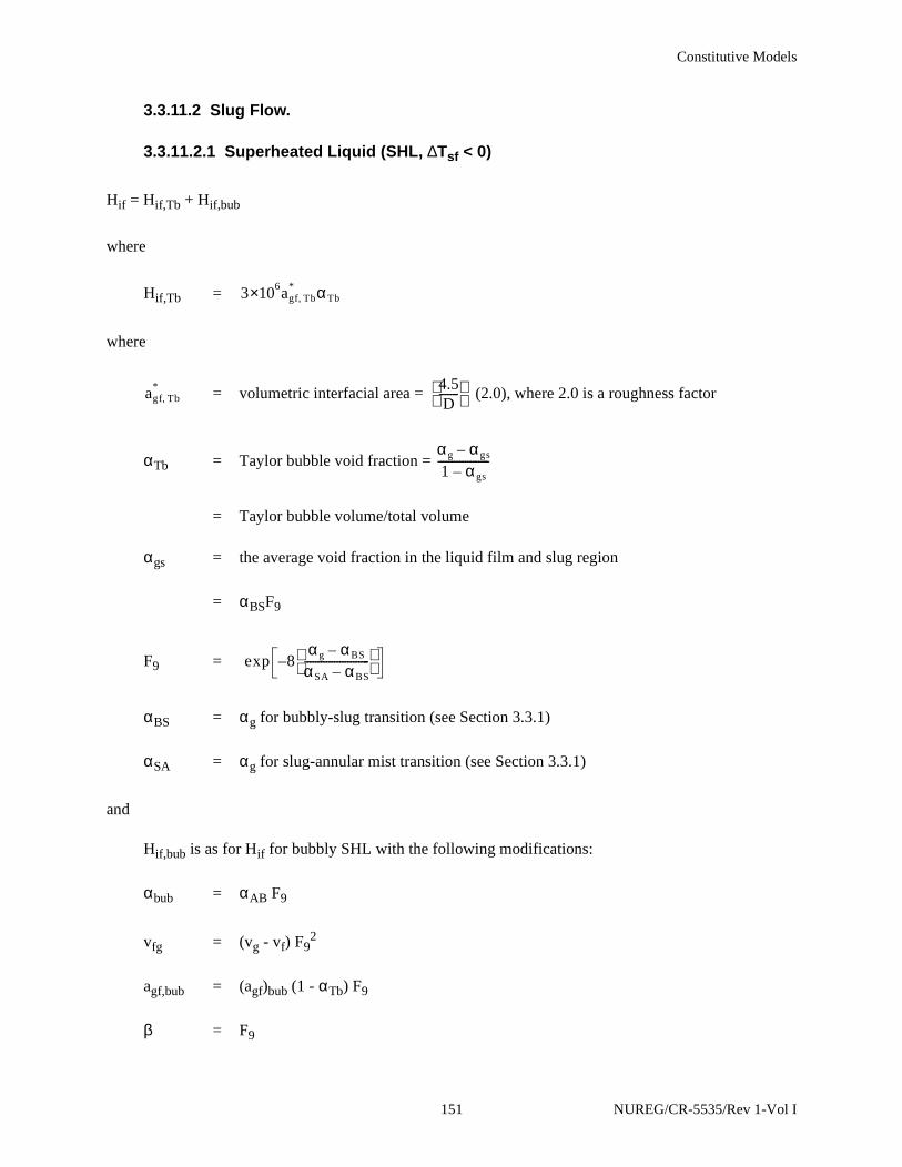
Constitutive Models
3.3.11.2 Slug Flow.
3.3.11.2.1 Superheated Liquid (SHL, ∆Tsf < 0)
Hif = Hif,Tb + Hif,bub
where
Hif,Tb =
where
= volumetric interfacial area = (2.0), where 2.0 is a roughness factor
αTb = Taylor bubble void fraction =
= Taylor bubble volume/total volume
αgs = the average void fraction in the liquid film and slug region
= αBSF9
F9 =
αBS = αg for bubbly-slug transition (see Section 3.3.1)
αSA = αg for slug-annular mist transition (see Section 3.3.1)
and
Hif,bub is as for Hif for bubbly SHL with the following modifications:
αbub = αAB F9
vfg = (vg - vf) F92
agf,bub = (agf)bub (1 - αTb) F9
β = F9
3 6×10 agf Tb,* αTb
agf Tb,* 4.5
D-------
αg αgs–1 αgs–-------------------
exp 8αg αBS–αSA αBS–------------------------
–
151 NUREG/CR-5535/Rev 1-Vol I

Constitutive Models
3.3.11.2.2 Subcooled Liquid (SCL, ∆Tsf > 0)
Hif = Hif,Tb + Hif,bub
where
Hif,Tb =
where
αTb and are as for slug SHL
Prf =
Ref =
and
Hif,bub is as for bubbly SCL.
3.3.11.2.3 Superheated Gas (SHG, ∆Tsg < 0)
Hig = Hig,Tb + Hig,bub
where
Hig,Tb =
where
and αTb are as for slug SHL
Reg =
and
Hig,bub = hig (1 - αTb) agf,bub
1.18942Ref0.5Prf
0.5kf
D----agf Tb,
* αTb
agf Tb,*
Cpfµf
kf-------------
ρfD vf vg–µf
----------------------------
2.2 0.82Reg0.5+( )
kg
D-----agf Tb,
* αTb
agf Tb,*
ρg vf vg– Dµg
-----------------------------
NUREG/CR-5535/Rev 1-Vol I 152
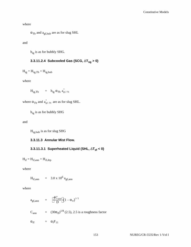
Constitutive Models
where
αTb and agf,bub are as for slug SHL
and
hig is as for bubbly SHG.
3.3.11.2.4 Subcooled Gas (SCG, ∆Tsg > 0)
Hig = Hig,Tb + Hig,bub
where
Hig,Tb = hig αTb
where αTb and are as for slug SHL.
hig is as for bubbly SHG
and
Hig,bub is as for slug SHG
3.3.11.3 Annular Mist Flow.
3.3.11.3.1 Superheated Liquid (SHL, ∆Tsf < 0)
Hif = Hif,ann + Hif,drp
where
Hif,ann = 3.0 x 10⁶ agf,ann
where
agf,ann =
Cann = (30αff)1/8 (2.5), 2.5 is a roughness factor
αff = αfF11
agf Tb,*
agf Tb,*
4Cann
D-------------
1 α ff–( )1 2⁄
153 NUREG/CR-5535/Rev 1-Vol I
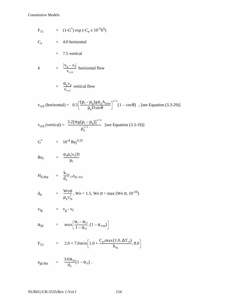
Constitutive Models
F11 = (1-G*) exp (-Ce x 10-5λ6)
Ce = 4.0 horizontal
= 7.5 vertical
λ = horizontal flow
= vertical flow
vcrit (horizontal) = , [see Equation (3.3-29)]
vcrit (vertical) = [see Equation (3.3-19)]
G* = 10-4 Ref0.25
Ref =
Hif,drp =
dd = , We = 1.5, We σ = max (We σ, 10-10)
vfg = vg - vf
αfd =
F13 =
agf,drp = .
vg vf–vcrit
------------------
αgvg
vcrit-----------
0.5ρf ρg–( )gαgApipe
ρgD θsin-------------------------------------------
1 2⁄1 θcos–( )
3.2 σg ρf ρg–( )[ ] 1 4⁄
ρg1 2⁄-----------------------------------------------
α fρf vf Dµf
----------------------
kf
dd-----F13agf drp,
Weσρgvfg
2------------
maxα f α ff–1 α ff–------------------ 1 α– AM( ),
2.0 7.0min 1.0Cpfmax 1.0 ∆Tsf,( )
hfg--------------------------------------------- 8.0,++
3.6α fd
dd--------------- 1 α ff–( )
NUREG/CR-5535/Rev 1-Vol I 154
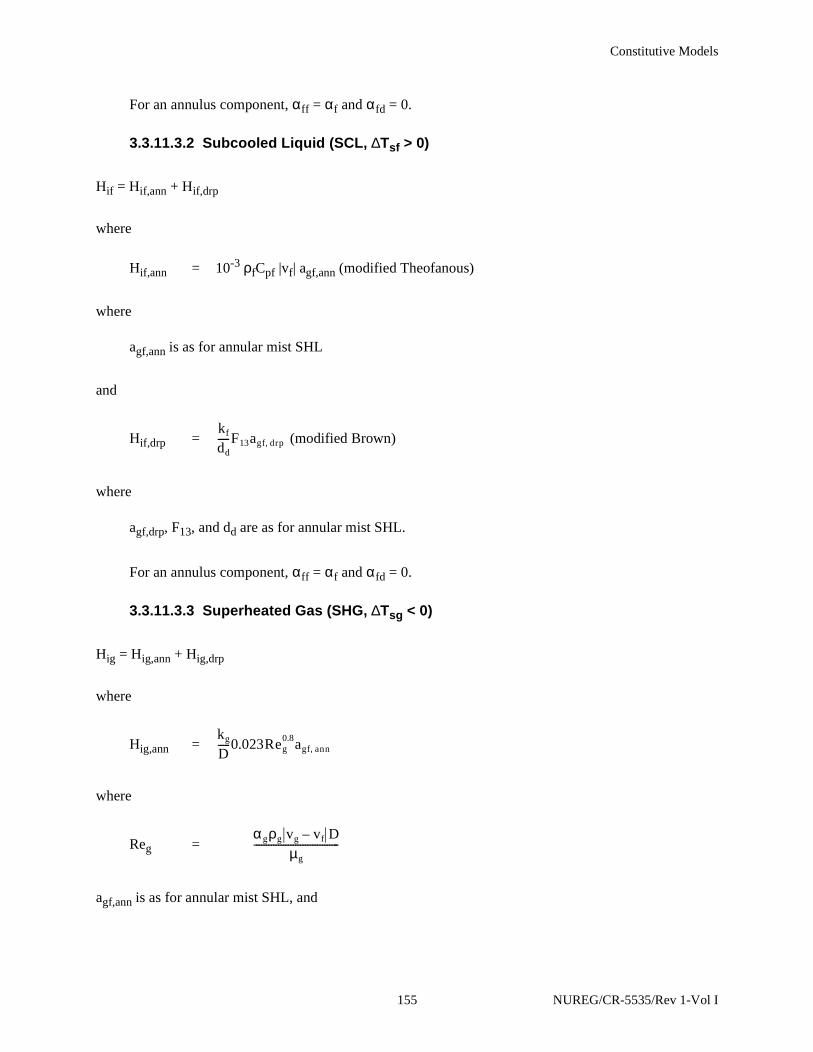
Constitutive Models
For an annulus component, αff = αf and αfd = 0.
3.3.11.3.2 Subcooled Liquid (SCL, ∆Tsf > 0)
Hif = Hif,ann + Hif,drp
where
Hif,ann = 10-3 ρfCpf |vf| agf,ann (modified Theofanous)
where
agf,ann is as for annular mist SHL
and
Hif,drp = (modified Brown)
where
agf,drp, F13, and dd are as for annular mist SHL.
For an annulus component, αff = αf and αfd = 0.
3.3.11.3.3 Superheated Gas (SHG, ∆Tsg < 0)
Hig = Hig,ann + Hig,drp
where
Hig,ann =
where
Reg =
agf,ann is as for annular mist SHL, and
kf
dd-----F13agf drp,
kg
D-----0.023Reg
0.8agf ann,
αgρg vg vf– Dµg
-----------------------------------
155 NUREG/CR-5535/Rev 1-Vol I

Constitutive Models
(Lee-Riley)
where
dd is as for annular mist SHL
Red = , where We=1.5
agf,drp, αf,d, and vfg are as for annular mist SHL.
For an annulus component, αff = αf and αfd = 0.
3.3.11.3.4 Subcooled Gas (SCG, ∆Tsg > 0)
Hig = Hig,ann + Hig,drp
where
Hig,ann = higagf,ann
where hig is as for bubbly SHG and agf,ann is as for annular mist SHL
and
Hig,drp = hig agf,drp
where
hig is as for bubbly SHG and
agf,drp is as for annular mist SHG.
For an annulus component, αff = αf and αfd = 0.
3.3.11.4 Inverted Annular Flow.
3.3.11.4.1 Superheated Liquid (SHL, ∆Tsf < 0)
Hif = Hif,bub + Hif,ann
Hig drp,kg
dd----- 2.0 0.5Red
0.5+( )agf drp,=
1 α f d,–( )2.5ρgvfgdd
µg----------------------------------------------
Weσ 1 α f d,–( )2.5
µgvfg----------------------------------------=
NUREG/CR-5535/Rev 1-Vol I 156
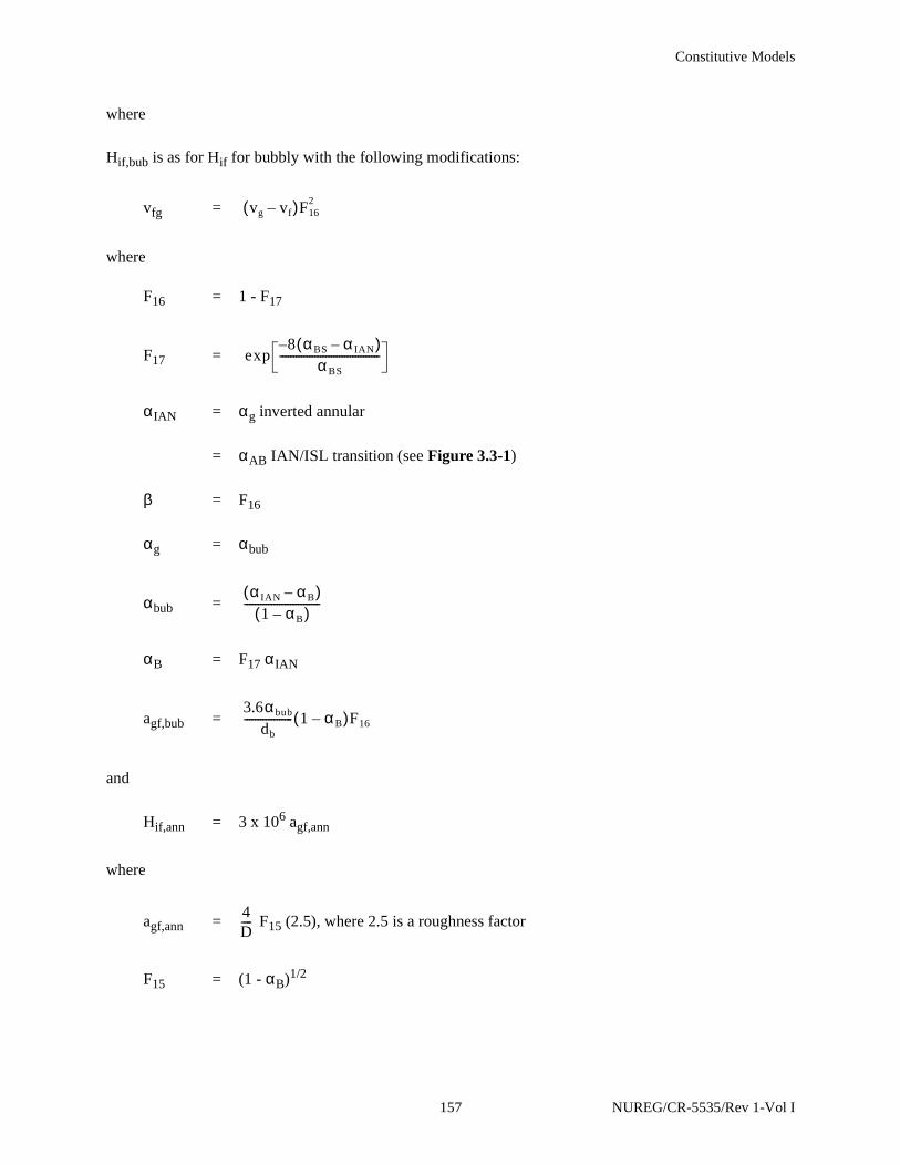
Constitutive Models
where
Hif,bub is as for Hif for bubbly with the following modifications:
vfg =
where
F16 = 1 - F17
F17 =
αIAN = αg inverted annular
= αAB IAN/ISL transition (see Figure 3.3-1)
β = F16
αg = αbub
αbub =
αB = F17 αIAN
agf,bub =
and
Hif,ann = 3 x 10⁶ agf,ann
where
agf,ann = F15 (2.5), where 2.5 is a roughness factor
F15 = (1 - αB)1/2
vg vf–( )F162
exp8 αBS α IAN–( )–
αBS-------------------------------------
α IAN αB–( )1 αB–( )
----------------------------
3.6αbub
db------------------ 1 αB–( )F16
4D----
157 NUREG/CR-5535/Rev 1-Vol I

Constitutive Models
3.3.11.4.2 Subcooled Liquid (SCL, ∆Tsf > 0)
Hif = Hif,bub + Hif,ann
where
Hif,bub is as for bubbly SCL
and
Hif,ann =
where
ReIAN =
agf,ann and αIAN are as for inverted annular SHL.
3.3.11.4.3 Superheated Gas (SHG, ∆Tsg < 0)
Hig = Hig,bub + Hig,ann
where
Hig,bub = hig agf,bub
where
hig is as for bubbly SHG and agf,bub is as for inverted annular SHL
and
Hig,ann = agf,ann
where
agf,ann is as for inverted annular SHL.
kf
D----0.023ReIAN
0.8 agf ann,
1 α IAN–( )ρf vf vg–
µf-----------------------
kg
D-----
NUREG/CR-5535/Rev 1-Vol I 158

Constitutive Models
3.3.11.4.4 Subcooled Gas (SCG, ∆Tsg > 0)
Hig is as for inverted annular SHG.
3.3.11.5 Inverted Slug Flow.
3.3.11.5.1 Superheated Liquid (SHL, ∆Tsf < 0)
Hif = Hif,ann + Hif,drp
where
Hif,ann = F13 agf,ann
where
agf,ann = αB(2.5), where 2.5 is a roughness factor
αB =
αdrp = (1 - αAM) F21
F21 =
and
Hif,drp = F13 agf,drp
where
agf,drp =
dd = characteristic droplet diameter
= , where We = 6.0
kf
D----
4.5D
-------
α f α drp–1 αdrp–--------------------
exp αAM α g–( )αAM αBS–( )
------------------------------–
kf
dd-----
3.6αdrp
dd----------------- 1 αB–( )
Weσρgvfg
2------------
159 NUREG/CR-5535/Rev 1-Vol I

Constitutive Models
vfg = (vg - vf) .
3.3.11.5.2 Subcooled Liquid (SCL, ∆Tsf > 0)
Hif = Hif,ann + Hif,drp
where
Hif,ann = F13 agf,ann
where
F13 is as for annular-mist SCL
agf,ann is as for inverted slug SHL
and
Hif,drp = F13 agf,drp
where
agf,drp is as for inverted slug SHL.
3.3.11.5.3 Superheated Gas (SHG, ∆Tsg < 0)
Hig = Hig,ann + Hig,drp
where
Hig,ann = agf,ann
where
agf,ann is as for inverted slug SHL
and
F212
kf
D----
kf
dd-----
kg
D-----
NUREG/CR-5535/Rev 1-Vol I 160
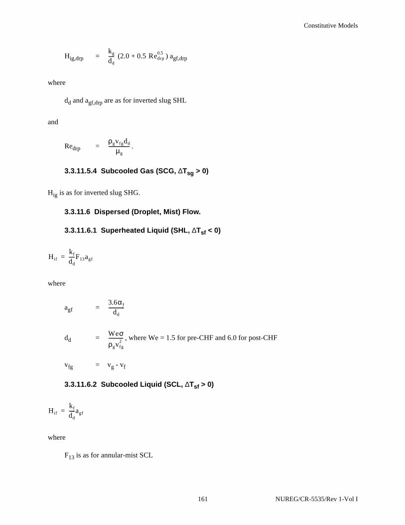
Constitutive Models
Hig,drp = (2.0 + 0.5 ) agf,drp
where
dd and agf,drp are as for inverted slug SHL
and
Redrp = .
3.3.11.5.4 Subcooled Gas (SCG, ∆Tsg > 0)
Hig is as for inverted slug SHG.
3.3.11.6 Dispersed (Droplet, Mist) Flow.
3.3.11.6.1 Superheated Liquid (SHL, ∆Tsf < 0)
where
agf =
dd = , where We = 1.5 for pre-CHF and 6.0 for post-CHF
vfg = vg - vf
3.3.11.6.2 Subcooled Liquid (SCL, ∆Tsf > 0)
where
F13 is as for annular-mist SCL
kg
dd----- Redrp
0.5
ρgvfgdd
µg-----------------
Hif
kf
dd-----F13agf=
3.6α f
dd-------------
Weσρgvfg
2------------
Hif
kf
dd-----agf=
161 NUREG/CR-5535/Rev 1-Vol I
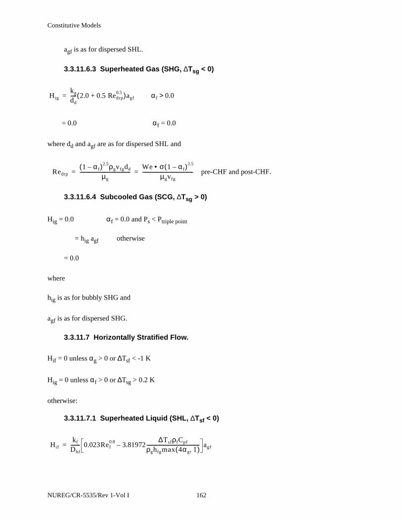
Constitutive Models
agf is as for dispersed SHL.
3.3.11.6.3 Superheated Gas (SHG, ∆Tsg < 0)
= 0.0 αf = 0.0
where dd and agf are as for dispersed SHL and
3.3.11.6.4 Subcooled Gas (SCG, ∆Tsg > 0)
Hig = 0.0 αf = 0.0 and Ps < Ptriple point
= hig agf otherwise
= 0.0
where
hig is as for bubbly SHG and
agf is as for dispersed SHG.
3.3.11.7 Horizontally Stratified Flow.
Hif = 0 unless αg > 0 or ∆Tsf < -1 K
Hig = 0 unless αf > 0 or ∆Tsg > 0.2 K
otherwise:
3.3.11.7.1 Superheated Liquid (SHL, ∆Tsf < 0)
Hig
kg
dd----- 2.0 0.5 Redrp
0.5+( )agf α f 0.0>=
Redrp
1 α f–( )2.5ρgvfgdd
µg------------------------------------------
We σ 1 α f–( )2.5•µgvfg
------------------------------------------ pre-CHF and post-CHF.= =
Hif
kf
Dhf-------- 0.023Ref
0.8 3.81972∆TsfρfCpf
ρghfgmax 4αg 1,( )--------------------------------------------– agf=
NUREG/CR-5535/Rev 1-Vol I 162

Constitutive Models
where
Dhf = liquid phase hydraulic diameter
= (see Figure 3.1-2 for definition of θ)
Ref =
agf =
F27 =
3.3.11.7.2 Subcooled Liquid (SCL, ∆Tsf > 0)
where
Dhf, Ref and agf are as for horizontally stratified SHL.
3.3.11.7.3 Superheated Gas (SHG, ∆Tsg < 0)
where
Dhg = vapor phase hydraulic diameter
=
Reg =
hig is as for bubbly SHG, and agf is as for horizontally stratified SHL.
παfDπ θ– θsin+-----------------------------
α fρf vg vf– Dµf
----------------------------------
4 θsinπD
--------------F27
1 vg vf–vcrit
---------------1 2⁄
+
Hif
kf
Dhf-------- 0.023Ref
0.8( )agf=
Hig
kg
Dhg-------- 0.023Reg
0.8 4higmax 0.0 0.25 αg–,( )+[ ] agf=
παgDθ θsin+--------------------
αgρg vg vf– Dµg
-----------------------------------
163 NUREG/CR-5535/Rev 1-Vol I

Constitutive Models
3.3.11.7.4 Subcooled Gas (SCG, ∆Tsg > 0)
Hig = hig agf
where
hig is as for bubbly SHG and
agf is as for horizontally stratified SHL.
3.3.11.8 Vertically Stratified Flow.
3.3.11.8.1 Superheated Liquid (SHL, ∆Tsf < 0)
Hif = Hif,REG
where
REG = flow regime of flow when not vertically stratified, which can be BBY, SLG,SLG/ANM, MPR, ANM, IAN, IAN/ISL, MST, ISL, MPO, IAN/ISL - SLG,ISL-SLG/ANM, ANM/MST, BBY/IAN, SLG/ISL (see flow regime map,Figure 3.3-1)
3.3.11.8.2 Subcooled Liquid (SCL, ∆Tsf > 0)
(McAdams)
where
agf =
L = length of volume cell
Nu = 0.27 (GrPr)0.25
3.3.11.8.3 Superheated Gas (SHG, ∆Tsg < 0)
where
Hif Nukf
D----agf=
AV----
AAL--------
1L---= =
Hig Nukg
D-----agf=
NUREG/CR-5535/Rev 1-Vol I 164

Constitutive Models
Nu = 0.27 (GrPr)0.25
agf =
agf is as for vertically stratified SHL.
3.3.11.8.4 Subcooled Gas (SCG, ∆Tsg > 0)
Hig = Hig,REG
3.3.12 Direct Heating
The direct (sensible) heating between the gas and liquid becomes important when there is
noncondensable present (see Section 3.1.1.2). This occurs when Ps < P. The direct heat transfer coefficient
is
(3.3-214)
Thus, when the gas is subcooled, Hgf uses the value of Hig at saturation.
3.3.13 References
3.3-1. W. L. Weaver et al. TRAC-BF1 Manual: Extensions to TRAC-BD1/MOD1. NUREG/CR-4391,EGG-2417. Idaho National Engineering Laboratory. August 1986.
3.3-2. D. D. Taylor et al. TRAC-BD1/MOD1: An Advanced Best Estimate Computer Program forBoiling Water Reactor Transient Analysis, Volume I: Model Description. NUREG/CR-3633,EGG-2294. Idaho National Engineering Laboratory. April 1984.
3.3-3. Y. Taitel and A. E. Dukler. “A Model of Predicting Flow Regime Transitions in Horizontal andNear Horizontal Gas-Liquid Flow.” AIChE Journal. 22. 1976. pp. 47-55.
3.3-4. Y. Taitel, D. Bornea, and A. E. Dukler. “Modeling Flow Pattern Transitions for Steady UpwardGas-Liquid Flow in Vertical Tubes.” AIChE Journal. 26. 1980. pp. 345-354.
3.3-5. M. Ishii and G. De Jarlais. “Inverted Annular Flow Modeling.” Advanced Code Review GroupMeeting, Idaho Falls, ID. July 27, 1982.
3.3-6. M. Ishii and T. C. Chawla. Local Drag Laws in Dispersed Two-Phase Flow. NUREG/CR-1230,ANL-79-105. Argonne National Laboratory. 1979.
AV----
AAL--------
1L---= =
Hgf
Hig Tg Ts>( ) Tg Ts>
Hig Tg Ts=( ) Tg Ts≤
=
165 NUREG/CR-5535/Rev 1-Vol I
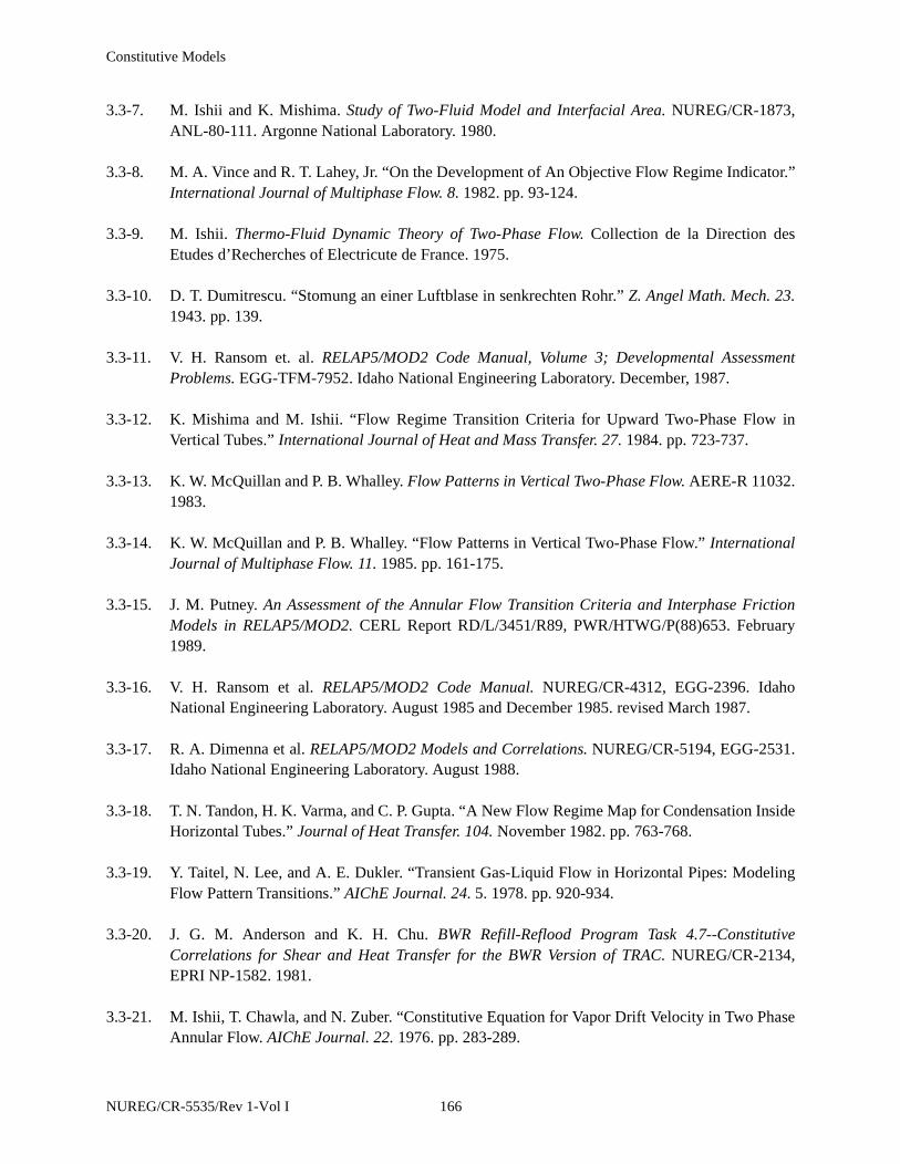
Constitutive Models
3.3-7. M. Ishii and K. Mishima. Study of Two-Fluid Model and Interfacial Area. NUREG/CR-1873,ANL-80-111. Argonne National Laboratory. 1980.
3.3-8. M. A. Vince and R. T. Lahey, Jr. “On the Development of An Objective Flow Regime Indicator.”International Journal of Multiphase Flow. 8. 1982. pp. 93-124.
3.3-9. M. Ishii. Thermo-Fluid Dynamic Theory of Two-Phase Flow. Collection de la Direction desEtudes d’Recherches of Electricute de France. 1975.
3.3-10. D. T. Dumitrescu. “Stomung an einer Luftblase in senkrechten Rohr.” Z. Angel Math. Mech. 23.1943. pp. 139.
3.3-11. V. H. Ransom et. al. RELAP5/MOD2 Code Manual, Volume 3; Developmental AssessmentProblems. EGG-TFM-7952. Idaho National Engineering Laboratory. December, 1987.
3.3-12. K. Mishima and M. Ishii. “Flow Regime Transition Criteria for Upward Two-Phase Flow inVertical Tubes.” International Journal of Heat and Mass Transfer. 27. 1984. pp. 723-737.
3.3-13. K. W. McQuillan and P. B. Whalley. Flow Patterns in Vertical Two-Phase Flow. AERE-R 11032.1983.
3.3-14. K. W. McQuillan and P. B. Whalley. “Flow Patterns in Vertical Two-Phase Flow.” InternationalJournal of Multiphase Flow. 11. 1985. pp. 161-175.
3.3-15. J. M. Putney. An Assessment of the Annular Flow Transition Criteria and Interphase FrictionModels in RELAP5/MOD2. CERL Report RD/L/3451/R89, PWR/HTWG/P(88)653. February1989.
3.3-16. V. H. Ransom et al. RELAP5/MOD2 Code Manual. NUREG/CR-4312, EGG-2396. IdahoNational Engineering Laboratory. August 1985 and December 1985. revised March 1987.
3.3-17. R. A. Dimenna et al. RELAP5/MOD2 Models and Correlations. NUREG/CR-5194, EGG-2531.Idaho National Engineering Laboratory. August 1988.
3.3-18. T. N. Tandon, H. K. Varma, and C. P. Gupta. “A New Flow Regime Map for Condensation InsideHorizontal Tubes.” Journal of Heat Transfer. 104. November 1982. pp. 763-768.
3.3-19. Y. Taitel, N. Lee, and A. E. Dukler. “Transient Gas-Liquid Flow in Horizontal Pipes: ModelingFlow Pattern Transitions.” AIChE Journal. 24. 5. 1978. pp. 920-934.
3.3-20. J. G. M. Anderson and K. H. Chu. BWR Refill-Reflood Program Task 4.7--ConstitutiveCorrelations for Shear and Heat Transfer for the BWR Version of TRAC. NUREG/CR-2134,EPRI NP-1582. 1981.
3.3-21. M. Ishii, T. Chawla, and N. Zuber. “Constitutive Equation for Vapor Drift Velocity in Two PhaseAnnular Flow. AIChE Journal. 22. 1976. pp. 283-289.
NUREG/CR-5535/Rev 1-Vol I 166

Constitutive Models
3.3-22. M. Ishii. One-Dimensional Drift-Flux Model and Constitutive Equations for Relative MotionBetween Phases in Various Two-Phase Flow Regimes. ANL-77-47. Argonne NationalLaboratory. 1977.
3.3-23. G. B. Wallis. One-Dimensional Two-Phase Flow. New York: McGraw-Hill Book Company.1969.
3.3-24. A. H. Shapiro and A. J. Erickson. Transactions of ASME. 79. 1957. pp. 775.
3.3-25. J. M. Putney. Proposals for Improving Interphase Drag Modeling for the Bubbly and SlugRegimes in RELAP5. CERL Report RD/L/3306/R88, PWR/HTWG/P(88)622. June 1988.
3.3-26. J. M. Putney. Implementation of a New Bubbly-Slug Interphase Drag Model in RELAP5/MOD2.CERL Report RD/L/3369/R88, PWR/HTWG/P(88)597. November 1988.
3.3-27. J. M. Putney. Equations for Calculating Interfacial Drag and Shear from Void FractionCorrelations. CERL Report RD/L/3429/R88, PWR/HTWG/P(88)630. December 1988.
3.3-28. J. M. Putney. Development of a New Bubbly-Slug Interfacial Friction Model for RELAP5--FinalReport. National Power Report ESTD/L/0075/R89, PWR/HTWG/P(89)722. October 1989.
3.3-29. J. M. Putney. Development of a New Bubbly-Slug Interfacial Friction Model for RELAP5.Nuclear Engineering and Design. 131. 1991. pp. 223-240.
3.3-30. B. Chexal and G. Lellouche. A Full-Range Drift-Flux Correlation for Vertical Flows (Revision1). EPRI NP-3989-SR. September 1986.
3.3-31. B. Chexal et al. The Chexal-Lellouche Void Fraction Correlation for Generalized Applications.NSAC-139. April 1991.
3.3-32. N. Zuber and J. Findlay. “Average Volumetric Concentrations in Two-Phase Flow Systems.”Journal of Heat Transfer. 87. 1965. pp. 453-568.
3.3-33. N. Zuber et al. Steady-State and Transient Void Fraction in Two-Phase Flow Systems. GEAP-5417. 1967.
3.3-34. I. Kataoka and M. Ishii. “Drift Flux Model for Large Diameter Pipe and New Correlation forPool Void Fraction.” International Journal of Heat Mass Transfer. 30. 1987. pp. 1927-1939.
3.3-35. S. Rouhani. Modified Correlations for Void and Pressure Drop. AB Atomenergi: Sweden.Internal Report AE-RTC 841. March 1969.
3.3-36. S. Rouhani et al. TRAC-BF1 Models and Correlations. NUREG/CR-4391, EGG-2680. IdahoNational Engineering Laboratory. August 1992.
167 NUREG/CR-5535/Rev 1-Vol I

Constitutive Models
3.3-37. G. B. Wallis and S. Makkenchey. “The Hanging Film Phenomenon in Vertical Annular Two-Phase Flow.” Transactions ASME, Series I. 96. 1974. P.. 297.
3.3-38. J. A. Holmes. “Description of the Drift Flux Model in the LOCA Code RELAP-UK.” I. Mech.E.. C206/77. 1977.
3.3-39. V. H. Ransom et al. RELAP5/MOD1 Code Manual. NUREG/CR-1826, EGG-2070. IdahoNational Engineering Laboratory. March 1982.
3.3-40. D. Bharathan, G. B. Wallis, and H. J. Richter. Air-Water Counter-Current Annular Flow. EPRI/NP-1165. 1979.
3.3-41. G. DeJarlais and M. Ishii. Inverted Annular Flow Experimental Study. NUREG/CR-4277, ANL-85-31. Argonne National Laboratory. April 1985.
3.3-42. N. Zuber. “On the Dispersed Two-Phase Flow in the Laminar Flow Regime.” ChemicalEngineering Science. 19. 1964. pp. 897-917.
3.3-43. D. A. Drew, L. Y. Cheng, and R. T. Lahey, Jr. “The Analysis of Virtual Mass Effects in Two-Phase Flow.” International Journal of Multiphase Flow. 5. 1979. pp. 233-242.
3.3-44. K. T. Chaxton, J. G. Collier, and J. A. Ward. H.T.F.S. Correlation for Two-Phase Pressure Dropand Void Fraction in Tubes. AERE-R7162. 1972.
3.3-45. D. Chisholm. “A Theoretical Basis for the Lockhart-Martinelli Correlation for Two-Phase Flow.”Journal of Heat-Mass Transfer. 10. 1967. pp. 1767-1778.
3.3-46. R. W. Lockhart and R. C. Martinelli. “Proposed Correlation of Data for Isothermal Two-Phase,Two-Component Flow in Pipes.” Chemical Engineering Progress. 45. 1. 1949. pp. 39-48.
3.3-47. C. F. Colebrook. “Turbulent Flow in Pipes with Particular Reference to the Transition RegionBetween Smooth and Rough Pipe Laws.” Journal of Institute of Civil Engineers. 11. 1939. pp.133-156.
3.3-48. D. J. Zigrang and N. D. Sylvester. “A Review of Explicit Friction Factor Equations.”Transactions of ASME, Journal of Energy Resources Technology. 107. 1985. pp. 280-283.
3.3-49. C. W. Stewart et al. VIPRE-01: A Thermal-Hydraulic Code for Reactor Cores. EPRI NP-2511-CCM. July 1985.
3.3-50. W. M. Rosenhow and J. P. Hartnett (eds.). Handbook of Heat Transfer. New York NY: McGraw-Hill. 1973.
3.3-51. J. C. Chen. “A Correlation for Boiling Heat Transfer to Saturated Fluids in Convective Flow.”Process Design and Development. 5. 1966. pp. 322-327.
NUREG/CR-5535/Rev 1-Vol I 168

Constitutive Models
3.3-52. D. C. Groeneveld, S. C. Cheng, and T. Doan. “1986 AECL-UO Critical Heat Flux LookupTable.” Heat Transfer Engineering. 7. 1-2. 1986. pp. 46-62.
3.3-53. R. Pernicia and J. Cizek. “General Correlation for Prediction of Critical Heat Flux Ratio.”Proceedings of the 7th International Meeting on Nuclear Reactor Thermal-Hydraulics,NURETH-7, Saratoga Springs, NY, September 10 - 15, 1995. NUREG/CP-0142. Vol. 4.
3.3-54. J. C. Chen, R. K. Sundaram, and F. T. Ozkaynak. A Phenomenological Correlation for Post-CHFHeat Transfer. NUREG-0237. June 1977.
3.3-55. L. A. Bromley. “Heat Transfer in Stable Film Boiling.” Chemical Engineering Progress. 46.1950. pp. 221-227.
3.3-56. R. T. Lahey. “A Mechanistic Subcooled Boiling Model.” Proceedings Sixth International HeatTransfer Conference, Toronto, Canada. 1978. Volume 1. pp. 293-297.
3.3-57. P. Saha and N. Zuber. “Point of Net Vapor Generation and Vapor Void Fraction in SubcooledBoiling.” Proceedings Fifth International Heat Transfer Conference, Vol. 4, 1974. pp. 175-179.
3.3-58. F. W. Dittus and L. M. K. Boelter. “Heat Transfer in Automobile Radiators of the Tubular Type.”Publications in Engineering. 2. University of California-Berkeley. 1930. pp. 443-461.
3.3-59. W. M. Kays. “Numerical Solution for Laminar Flow Heat Transfer in Circular Tubes.”Transactions, American Society of Mechanical Engineers. 77. 1955. pp. 1265-1274.
3.3-60. S. W. Churchill and H. H. S. Chu. “Correlating Equations for Laminar and Turbulent FreeConvection from a Vertical Plate.” International Journal of Heat and Mass Transfer. 18. 1975.pp. 1323-1329.
3.3-61. B. S. Petukhov. “Heat Transfer and Friction in Turbulent Pipe Flow with Variable PhysicalProperties.” Advances in Heat Transfer. New York: Academic Press. 1970. pp. 503-565.
3.3-62. F. P. Incropera and D. P. DeWitt. Introduction to Heat Transfer. New York: John Wiley & Sons.1990. pp. 501.
3.3-63. A. Y. Inayatov. “Correlation of Data on Heat Transfer Flow Parallel to Tube Bundles at RelativeTube Pitches of 1.1 < s/d < 1.6.” Heat Transfer-Soviet Research. 7. 3. May-June 1975.
3.3-64. G. T. Polley, T. Ralston, and I. D. R. Grant. “Forced Crossflow Boiling in an Ideal In-line TubeBundle.” ASME 80-HT-46. 1981.
3.3-65. B. S. Folkin and Y. N. Goldberg. “Simulation of Free Convection Boiling Crisis In VaporBlanketing of a Horizontal Tube Bundle.” Heat Transfer Soviet Research. 12. 3. 1980. pp.77-81.
169 NUREG/CR-5535/Rev 1-Vol I

Constitutive Models
3.3-66. S. W. Churchill and H. H. S. Chu. “Correlating Equations for Laminar and Turbulent FreeConvection from a Horizontal Cylinder.” International Journal of Heat and Mass Transfer. 18.1975. pp. 1049.
3.3-67. W. Nusselt. “Die Oberflachenkondensation des Wasserdampfes.” Ver. deutsch. Ing.. 60. 1916.p. 541.
3.3-68. M. M. Shah. “A General Correlation for Heat Transfer during Film Condensation Inside Pipes.”International Journal of Heat and Mass Transfer. 22. 1979. pp. 547-556.
3.3-69. A. P. Colburn and O. A. Hougen. “Design of Cooler Condensers for Mixtures of Vapors withNon-Condensing Gases.” Industrial and Engineering Chemistry. 26. 1934. pp. 1178-1182.
3.3-70. K. M. Vierow and V. E. Schrock. “Condensation in a Natural Circulation Loop withNoncondensable Gas Present.” Japan-U. S. Seminar on Two-Phase Flow Dynamics, Berkeley,California, USA. 1992.
3.3-71. G. Th. Analytis. “Developmental Assessment of RELAP5/MOD3.1 with Separate Effect andIntegral Test Experiments: Model Changes and Options.” Nuclear Engineering and Design. 163.1996. pp. 125-148.
3.3-72. M. S. Plesset and S. A. Zwick. “Growth of Vapor Bubbles in Superheated Liquids.” Journal ofApplied Physics. 25. 4. 1954. pp. 493-500.
3.3-73. K. Lee and D. J. Ryley. “The Evaporation of Water Droplets in Superheated Steam.”Transactions of ASME, Journal of Heat Transfer. November 1968. pp. 445-456.
3.3-74. H. C. Unal. “Maximum Bubble Diameter, Maximum Bubble-Growth Time and Bubble-Growth
Rate During the Subcooled Nucleate Flow Boiling of Water up to 17.7 MN/m2). InternationalJournal of Heat Mass Transfer. 19. 1976. pp. 643-649.
3.3-75. R. A. Riemke. “Modification to Unal’s Subcooled Flow Boiling Bubble Model.” NuclearTechnology. 102. 1993. pp. 416-417.
3.3-76. G. Brown. “Heat Transmission by Condensation of Steam on a Spray of Water Drops.” Instituteof Mechanical Engineers. 1951. pp. 49-52.
3.3-77. T. G. Theofanous. “Modeling of Basic Condensation Processes.” The Water Reactor SafetyResearch Workshop on Condensation, Silver Springs, MD. May 24-25. 1979.
NUREG/CR-5535/Rev 1-Vol I 170

Special Process Models
3.4 Special Process Models
Certain models in RELAP5 have been developed to simulate special processes. These models are
described in the following subsections.
3.4.1 Choked Flow
A choked-flow model developed by Ransom and Trapp3.4-1,3.4-2 is included primarily for calculation
of the mass discharge from the system at a pipe break or a nozzle. Generally, the flow at the break or
nozzle is choked until the system pressure nears the containment pressure. The choked-flow model is used
to predict if the flow is choked at a break or nozzle and, if it is, to establish the discharge boundary
condition. In addition, the choked-flow model can be used to predict existence of and calculate choked
flow at internal points in the system.
Choking is defined as the condition wherein the mass flow rate becomes independent of the
downstream conditions (that point at which further reduction in the downstream pressure does not change
the mass flow rate). The fundamental reason that choking occurs is that acoustic signals can no longer
propagate upstream. This occurs when the fluid velocity equals or exceeds the propagation velocity. The
choked-flow model is based on a definition that is established by a characteristic analysis using time-
dependent differential equations.
Consider a system of n first-order, quasi-linear, partial differential equations of the form
(3.4-1)
The characteristic directions (or characteristic velocities) of the system are defined3.4-3,3.4-4 as the
roots, λj(i < n), of the characteristic polynomial
(3.4-2)
The real part of any root, λj, gives the velocity of signal propagation along the corresponding
characteristic path in the space/time plane. The imaginary part of any complex root, λj, gives the rate of
growth or decay of the signal propagating along the respective path. For a hyperbolic system in which all
the roots of Equation (3.4-2) are real and nonzero, the number of boundary conditions required at any
boundary point equals the number of characteristic lines entering the solution region as time increases. If
we consider the system [Equation (3.4-1)] for a particular region 0 < x < L and examine the boundary
conditions at x = L, as long as any λj are less than zero, we must supply some boundary information to
obtain the solution. If all λj are greater than or equal to zero, no boundary conditions are needed at x = L;
and the interior solution is unaffected by conditions beyond this boundary.
A U( )∂U∂t------- B U( )∂U
∂x------- C U( )+ + 0=
Aλ B–( ) 0=
171 NUREG/CR-5535/Rev 1-Vol I

Special Process Models
A choked condition exists when no information can propagate into the solution region from the
exterior. Such a condition exists at the boundary point, x = L, when
λj > 0 for all j < n (3.4-3)
These are the mathematical conditions satisfied by the equations of motion for a flowing fluid when
reduction in downstream pressure ceases to result in increased flow rate. It is well known3.4-5 that the
choked condition for single-phase flow occurs when the fluid velocity just equals the local sound speed.
For this case, one of the λj’s is just equal to zero. For the two-phase case, it is possible for all λj’s to be
greater than zero under special conditions which can exist during discharge of a subcooled liquid.
Extensive investigation was carried out to determine a two-phase choked-flow criterion under two
assumed conditions:a (a) thermal equilibrium between phases, and (b) adiabatic phases without phase
change (frozen).3.4-6 The frozen assumption was in poor agreement with data compared to the thermal
equilibrium assumption. Therefore, the thermal equilibrium assumption with slip is used as the basis for
the RELAP5 choked-flow criterion when two conditions exist.
3.4.1.1 Choking Criterion for Nonhomogeneous, Equilibrium Two-Phase Flow.
The two-fluid model for the conditions of thermal equilibrium (equilibrium interphase mass transfer)
is described by the overall mass continuity equation, two-phasic momentum equations, and the mixture
entropy equation. This system of equations is
(3.4−4)
(3.4-5)
a. The hydrodynamic model is not based on either of these assumptions. However, the purpose of this analysis is simply to establish a criterion for a choked flow; thus, there is no conflict with the basic hydrodynamic model.
∂ αgρg α fρf+( )∂t
------------------------------------∂ αgρgvg α fρfvf+( )
∂x-----------------------------------------------+ 0=
αgρg
∂vg
∂t-------- vg
∂vg
∂x--------+
αg∂P∂x------+
Cα gα fρ∂vg
∂t-------- vf
∂vg
∂x--------
∂vf
∂t-------– vg
∂vgf
∂x----------–+
+ 0=
NUREG/CR-5535/Rev 1-Vol I 172

Special Process Models
(3.4-6)
(3.4−7)
The momentum equations include the interphase force terms due to relative acceleration.3.4-7 These
force terms have a significant effect on wave propagation velocity and consequently on the choked flow
velocity. The particular form chosen is frame invariant and symmetrical; and the coefficient of virtual
mass, Cαgαfρ, is chosen to ensure a smooth transition between pure vapor and pure liquid. For a dispersed
flow, the constant, C, has a theoretical value of 0.5; whereas for a separated flow, the value may approach
zero. The energy equation is written in terms of mixture entropy, which is constant for adiabatic flow. (The
energy dissipation associated with interphase mass transfer and relative phase acceleration is neglected.)
The nondifferential source terms, C(U), in Equation (3.4-1) do not enter into the characteristic
analysis or affect the propagation velocities. For this reason, the source terms associated with wall friction,
interphase drag, and heat transfer are omitted for brevity in Equation (3.4-4) through (3.4-7).
In the thermal equilibrium case, ρg, ρf, Sg, and Sf are known functions of the pressure only (the vapor
and liquid values along the saturation curve). The derivatives of these variables are designated by an
asterisk as follows
(3.4−8)
(3.4-9)
The system of governing equations [Equation (3.4-4) through (3.4-7)] can be written in terms of the
four dependent variables, αg, P, vg, and vf, by application of the chain rule and the property derivatives
[Equation (3.4-8) and (3.4-9)]. Thus, the system of equations can be written in the form of Equation (3.4-1)
where the A and B are fourth-order square coefficient matrices.
The characteristic polynomial that results is fourth-order in λ, and factorization can only be carried
out approximately to obtain the roots for λ and establish the choking criterion. The first two roots are
α fρf
∂vf
∂t------- vf
∂vf
∂x-------+
α f∂P∂x------+
Cα fα gρ∂vf
∂t------- vg
∂vf
∂x-------
∂vg
∂t--------– vf
∂vg
∂x--------–+
+ 0=
∂ α gρgSg α fρfSf+( )∂t
-----------------------------------------------∂ α gρgSgvg α fρfSfvf+( )
∂x----------------------------------------------------------+ 0=
ρf* dρf
s
dP-------- ρ, g
* dρgs
dP--------= =
Sf* dSf
s
dP-------- S, g
* dSgs
dP--------= =
173 NUREG/CR-5535/Rev 1-Vol I

Special Process Models
(3.4−10)
These two roots are obtained by neglecting the fourth-order factors relative to the second-order
factors in (λ - vg) and (λ - vf). There are no first- or third-order factors. Inspection of Equation (3.4-10)
shows that λ1,2 have values between vg and vf; thus, the fourth-order factors, (λ - vg) and (λ - vf), are small
(i.e., neglecting these terms is justified). The values for λ1,2 may be real or complex depending on the sign
of the quantity .
The remaining two roots are obtained by dividing out the quadratic factor containing λ1,2, neglecting
the remainder, and factoring the remaining quadratic terms. [This procedure can be shown to be analogous
to neglecting the second- and higher-order terms in the relative velocity, (vg - vf).] The remaining roots are
λ3,4 = v + D(vg - vf) + a (3.4-11)
where
v = (3.4-12)
a = (3.4-13)
and
(3.4-14)
The quantity, aHE, is the homogeneous equilibrium speed of sound. The roots, λ3,4, have only real
values.
λ1 2,
α fρgρC2
-------ρC2
-------
2
α gα fρgρf–1 2⁄
±+
vg
αgρfρC2
-------+−ρC2
-------
2
αgα fρgρf–1 2⁄
+
vf+
α fρgρC2
-------+ αgρf
ρC2
-------+ +
-------------------------------------------------------------------------------------------------------------------=
ρC2
-------
2
α gα fρgρf–
αgρgvg α fρfvf+ρ
--------------------------------------
aHE
Cρ2 ρ αgρf α fρg+( )+
Cρ2 ρgρf+-----------------------------------------------------
1 2⁄
D 0.5αgρf α fρg–( )
ρC α fρg α gρf+ +( )-----------------------------------------------
ρgρf α fρf αgρg–( )ρ ρgρf Cρ2+( )
------------------------------------------- aHE2 ρ αgρg
2Sg* α fρf
2Sf*+( )
ρgρf Sg Sf–( )-------------------------------------------------–+=
NUREG/CR-5535/Rev 1-Vol I 174

Special Process Models
The general nature and significance of these roots is revealed by applying the characteristic
considerations. The speed of propagation of small disturbances is related to the values of the characteristic
roots. In general, the velocity of propagation corresponds to the real part of a root, and the growth or
attenuation is associated with the complex part of the root. Choking will occur when the signal, which
propagates with the largest velocity relative to the fluid, is just stationary, i.e.,
λR = 0 for j < 4 (3.4-15)
and
λR > 0 for all i ≠ j (3.4-16)
The existence of complex roots for λ1,2 makes the initial boundary value problem ill-posed. This
problem has been discussed by many investigators,3.4-8,3.4-9 and the addition of any small, second-order
viscous effects renders the problem well-posed.3.4-8,3.4-10 The whole phenomenon of systems with mixed
orders of derivatives and a first-order system with the addition of a small, second-order term has been
discussed and analyzed by Whitham.3.4-4 He has shown that the second-order viscous terms give infinite
characteristic velocities. However, very little information is propagated along these characteristic lines;
and the bulk of the information is propagated along characteristic lines defined by the first-order system.
We conclude that the ill-posed nature of Equation (3.4-4) through (3.4-7) can be removed by the addition
of small, second-order viscous terms that have little effect upon the propagation of information. Therefore,
the choking criterion for the two-phase flow system analyzed here is established from Equation (3.4-15).
The explicit character of the choking criterion for the two-phase flow model defined by Equation
(3.4-4) through (3.4-7) is examined. Since the two roots, λ1,2, are between the phase velocities, vf and vg,
the choking criterion is established from the roots, λ3,4, and Equation (3.4-15). The choking criterion is
v + D(vg - vf) = + a (3.4-17)
The choking criterion can be rewritten in terms of the mass mean and relative Mach numbers
(3.4-18)
as
Mv + DMr = + 1 (3.4-19)
Mvva---, Mr
vg vf–a
---------------= =
175 NUREG/CR-5535/Rev 1-Vol I
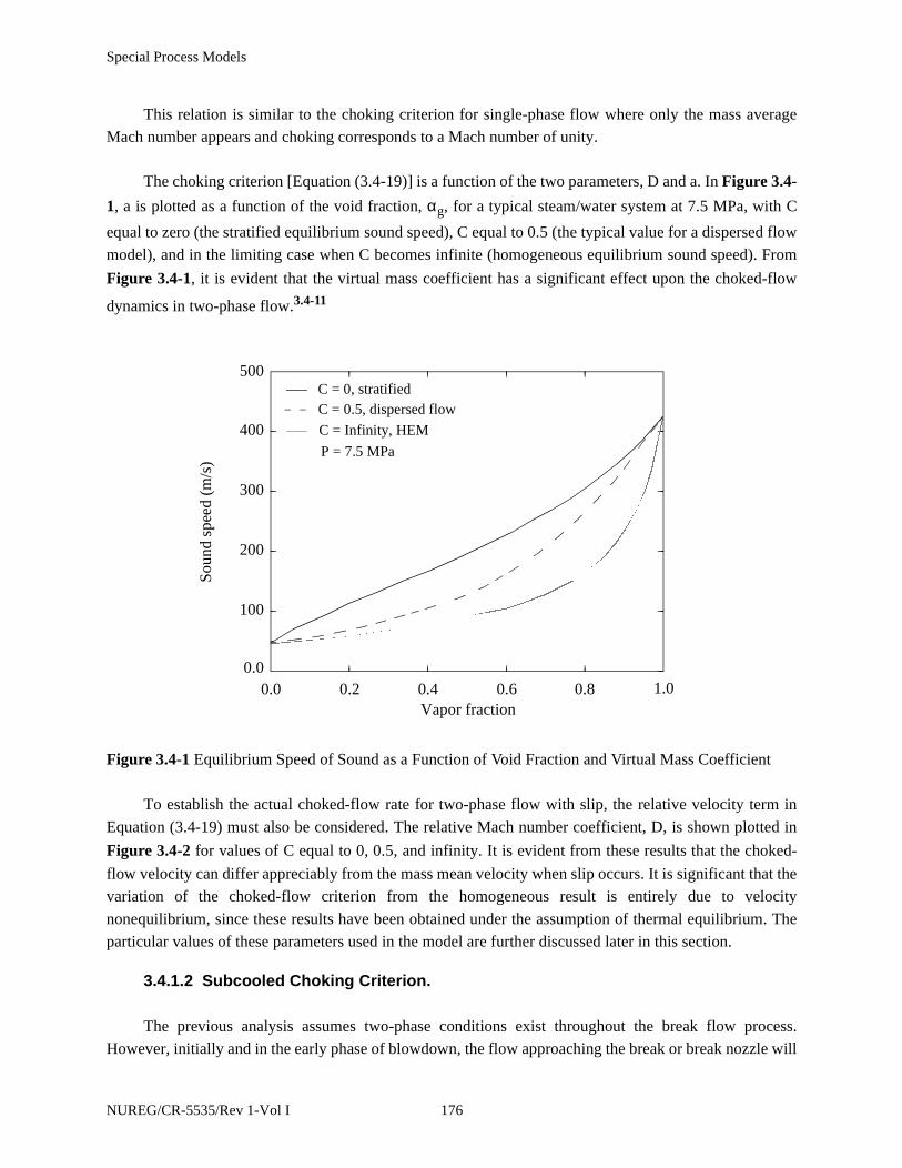
Special Process Models
This relation is similar to the choking criterion for single-phase flow where only the mass average
Mach number appears and choking corresponds to a Mach number of unity.
The choking criterion [Equation (3.4-19)] is a function of the two parameters, D and a. In Figure 3.4-
1, a is plotted as a function of the void fraction, αg, for a typical steam/water system at 7.5 MPa, with C
equal to zero (the stratified equilibrium sound speed), C equal to 0.5 (the typical value for a dispersed flow
model), and in the limiting case when C becomes infinite (homogeneous equilibrium sound speed). From
Figure 3.4-1, it is evident that the virtual mass coefficient has a significant effect upon the choked-flow
dynamics in two-phase flow.3.4-11
To establish the actual choked-flow rate for two-phase flow with slip, the relative velocity term in
Equation (3.4-19) must also be considered. The relative Mach number coefficient, D, is shown plotted in
Figure 3.4-2 for values of C equal to 0, 0.5, and infinity. It is evident from these results that the choked-
flow velocity can differ appreciably from the mass mean velocity when slip occurs. It is significant that the
variation of the choked-flow criterion from the homogeneous result is entirely due to velocity
nonequilibrium, since these results have been obtained under the assumption of thermal equilibrium. The
particular values of these parameters used in the model are further discussed later in this section.
3.4.1.2 Subcooled Choking Criterion.
The previous analysis assumes two-phase conditions exist throughout the break flow process.
However, initially and in the early phase of blowdown, the flow approaching the break or break nozzle will
Figure 3.4-1 Equilibrium Speed of Sound as a Function of Void Fraction and Virtual Mass Coefficient
0.0 0.2 0.4 0.6 0.8 1.0Vapor fraction
0.0
100
200
300
400
500
Sou
nd s
peed
(m
/s)
C = 0, stratifiedC = 0.5, dispersed flow
C = Infinity, HEM
P = 7.5 MPa
NUREG/CR-5535/Rev 1-Vol I 176

Special Process Models
be subcooled liquid. Under most conditions of interest in LWR systems, the fluid undergoes a phase
change at the break. The transition from single- to two-phase flow is accompanied by a discontinuous
change in the fluid bulk modulus. This is especially true for the liquid-to-liquid/vapor transition. For
example, at 600 KPa, the ratio of the single- to two-phase sound speed at the liquid boundary is 339.4.
Thus, considerable care must be exercised when analyzing a flow having transitions to or from a pure
phase. (A discontinuity is also present at the vapor boundary, but the ratio is only 1.069.)
To understand the physical process that occurs for subcooled upstream conditions, consider the flow
through a converging/diverging nozzle connected to an upstream plenum with subcooled water at a high
pressure. For a downstream pressure only slightly lower than the upstream pressure, subcooled liquid flow
will exist throughout the nozzle. Under these conditions, the flow can be analyzed using Bernoulli’s
equation, which predicts a minimum pressure, Pt, at the throat.a As the downstream pressure is lowered
further, a point is reached where the throat pressure equals the local saturation pressure, Psat. If the
downstream pressure is lowered further, vaporization will take place at the throat.b When this happens, the
Figure 3.4-2 Coefficient of Relative Mach Number for Thermal Equilibrium Flow as a Function of Void Fraction and Virtual Mass Coefficient
a. For all practical cases of choking, the subcooled water can be considered incompressible with infinite sound
speed.
b. An idealized one-dimensional homogeneous equilibrium model is assumed.
0.0 0.2 0.4 0.6 0.8 1.0Vapor fraction
-0.6
-0.3
0.0
0.3
0.6
Mac
h nu
mbe
r co
effi
cien
t
C = 0C = 0.5C = Infinity
P = 7.5 MPa
177 NUREG/CR-5535/Rev 1-Vol I
Special Process Models
fluid sound speed lowers drastically; but continuity considerations dictate that the velocity, vt, of the two-
phase mixture (at the point of minuscule void fraction) just equals the velocity of the subcooled water
slightly upstream of the throat. When this occurs, vt in the subcooled region is less than the water sound
speed; but in the two-phase region, vt can be greater than the two-phase sound speed. Hence, the subcooled
water has a Mach number (M) < 1, whereas the two-phase mixture at the throat has a Mach number > 1.
Under these conditions (Mach numbers > 1 in the two-phase region), downstream pressure effects are not
propagated upstream and the flow is choked. In particular, the supersonic two-phase fluid at the throat
must increase in velocity and the pressure must drop as it expands in the diverging section.a (Transition
back to subsonic flow can occur in the nozzle as a result of a shock wave.) This choked condition is shown
as case (a) in Figure 3.4-3. Contrary to the usual single-phase choked flow in a converging/diverging
nozzle, there is no point in the flow field where M = 1. This is because in the homogeneous equilibrium
model the fluid undergoes a discontinuous change in sound speed from single-phase subcooled conditions
to two-phase conditions, although the fluid properties are continuous through the transition point.
When this condition prevails, the flow rate can be established from application of Bernoulli’s
equation . For further decrease in the downstream pressure, no further
increase in upstream fluid velocity will occur as long as the upstream conditions are maintained constant.
Now consider the process where a subcooled choked flow, as described above, initially exists (with a
very low downstream pressure) and the upstream pressure is lowered as shown in cases (b) and (c) in
a. In a supersonic flow, a diverging nozzle implies an increase in velocity.
Figure 3.4-3 Subcooled Choking Process
thro
at
thro
at
thro
at
Psat
Pup(a)
Pup(b)
Pup(c)
(a) (b) (c)
M<1 M<1 M<1M>1 M>1M>1 M>1 M=1M=1
vt vup2
2Pup a( ) Psat–
ρ-----------------------------------
+1 2⁄
= vt vup2
2Pup b( ) Psat–
ρ-----------------------------------( )+
1 2⁄aHE= = vt aHE= vup
22
Pup c( ) Psat–
ρ-----------------------------------( )+
1 2⁄>
single-phase two-phase single-phase single-two-phase two-
Pup(b)
Pup(c)
phasephase
1 2⁄( )ρ vt2 v– up
2( ) Pup Psat–=[ ]
NUREG/CR-5535/Rev 1-Vol I 178
Special Process Models
Figure 3.4-3. As the upstream pressure decreases, the pressure at the throat will remain at Psat, and
Bernoulli’s equation will give a smaller subcooled water velocity (vt) at the throat. As Pup is lowered
further, a point is reached where vt = aHE and M = 1 on the two-phase side of the throat. (The Mach
number in the subcooled portion upstream of the throat is much less than 1.) This situation is shown
schematically in Figure 3.4-3 as case (b).
As the upstream pressure is lowered further, the point where the pressure reaches Psat must move
upstream of the throat. This is shown as case (c) in Figure 3.4-3. The subcooled water velocity at the Psat
location is smaller than the two-phase sound speed, and the flow is subsonic. In the two-phase region
between the point at which Psat is reached and the throat, the Mach number is less than 1 but increases to M
= 1 at the throat; that is, the two-phase sonic velocity is reached at the throat (as in the case of choked flow
having a continuous variation of sound speed with pressure). As Pup is lowered still further, the Psat point
moves upstream until the flow becomes completely two-phase.
The homogeneous assumption applied in the above subcooled choking description is very close to
the real situation when vapor is first formed. However, nonequilibrium can result in a superheated liquid
state at a throat pressure, Pt, much lower than the saturation pressure, Psat. The onset of vaporization occurs
at Pt instead of Psat.
The pressure undershoot, Psat - Pt, can be described by the Alamgir-Lienhard-Jones correlation3.4-
12,3.4-13,3.4-14
Psat - Pt = max (∆P, 0) (3.4-20)
with
(3.4−21)
The first term in ∆P represents the static depressurization effect and is derived by Alamgir and
Lienhard3.4-13 based on classical nucleation theory. For a steady flow in a nozzle, the depressurization rate,
∑′, can be shown to be
(3.4-22)
∆P 0.258σ3 2⁄ TR13.76 1 13.25RΣ′0.8+( )1 2⁄
kBTc( )1 2⁄ 1Vf
Vg------–
------------------------------------------------- 0.07
At
A-----
2
ρvc2( )–=
Σ′ρvc
3
At--------
dAdx-------
t
=
179 NUREG/CR-5535/Rev 1-Vol I

Special Process Models
Note that in Equation (3.4-21), ∑′ is in units of Matm/s, but in Equation (3.4-22), ∑′ is in units of
Pa/s. Here, is the variation of area with respect to axial length and is to be evaluated between the
center of the upstream volume and the throat. The second term in ∆P [Equation (3.4-22)] represents the
turbulence effect and is developed by Jones.3.4-14
The choking velocity, based upon the process shown in Figure 3.4-3, can be obtained in the
following manner. The subcooled critical flow model is based on the assumption that flashing occurs at the
throat of the nozzle or upstream of the throat. This assumption implies that critical flow of subcooled liquid
must be accompanied by a minimum pressure drop, which we denote by ∆Pmin. In this case ∆Pmin = Pup -
Pt, where Pup is the pressure in the upstream volume and Pt is the throat pressure obtained from the
Alamgir-Lienhard-Jones correlation. This leads to a condition on the fluid velocity at the throat, which is
obtained from the Bernoulli equation. Assuming the fluid is incompressible and that frictional and
gravitational forces are negligible, the Bernoulli equation is given by , where ∆P is
the pressure drop from the upstream volume to the throat, vt is the velocity at the throat, and vup is the
velocity in the upstream volume. Thus we obtain the condition vt > vc, where
(3.4-23)
and Pt is to be computed from Equation (3.4-20).
For the process shown in Figure 3.4-3 case (a), the choking velocity is given by Equation (3.4-23),
and for the process shown in Figure 3.4-3 case (b) and Figure 3.4-3 case (c), the two-phase choking
criterion applies and
vc = aHE (3.4-24)
where aHE is the equilibrium sound speed of a two-phase mixture.
To determine which of the above situations exists, both vc’s are calculated and the larger is used as
the choking velocity to be imposed at the throat. This velocity is imposed numerically in exactly the same
way as the choking criterion used for the two-phase condition described previously.
The equilibrium sound speed, aHE, is calculated using thermodynamic conditions at the throat.
Momentum and mechanical energy balances are used to calculate the pressure and internal energy at the
throat and use the water property tables to obtain the thermodynamic properties of a saturated liquid-vapor
mixture at this pressure and internal energy. This method is consistent with the process of subcooled
dAdx-------
t
∆P12---ρ vt
2 vup2–( )=
vc vup2 2
Pup Pt–ρ
------------------ +
1 2⁄
=
NUREG/CR-5535/Rev 1-Vol I 180
Special Process Models
critical flow described in this section, and allows for the presence of a two-phase mixture at the throat. The
precise equations used to determine the hydrodynamic conditions at the throat are presented in Volume IV.
Note that in an earlier version of RELAP5, the quality of the two-phase mixture at the throat was not
determined. Instead the throat was assumed to contain saturated liquid at the temperature of the subcooled
liquid upstream. However, this assumption led to an abrupt change of the computed flowrate at the single-
phase to two-phase transition.
The subcooled choking model is very similar in concept to the model proposed by Burnell3.4-15 in
that both models assume a Bernoulli expansion to the point of vapor inception at the choke plane. The
criterion for transition from subcooled choking to two-phase choking is now better understood and is in
agreement with the physics of two-phase flow. The model here is also in agreement with cavitating venturi
experience (experimentally confirmed behavior)3.4-12. The RELAP5 subcooled choking model is
somewhat different than the model proposed by Moody3.4-16 in that the Moody model assumes that an
isentropic process occurs to the choke plane.
3.4.1.3 Implementation of Choked Flow Model.
Ideally, the two-phase choking criterion [Equation (3.4-17)] can be used as a boundary condition for
obtaining flow solutions. However, the applicability of Equation (3.4-17) has not been fully explored.
Instead, an approximate criterion
(3.4-25)
has been applied extensively and has produced good code/data comparisons. Equation (3.4-25) can be
obtained from Equation (3.4-17) in the following manner. Neglecting the third term in D, we obtain
(3.4-26)
Then setting C = 0 (stratified) on the left side of Equation (3.4-26) and C = ∞ (homogeneous) on the
right side of Equation (3.4-26) and computing the limits, we obtain the approximate criterion given by
Equation (3.4-25). Because of the extensive experience with this approximate model, Equation (3.4-25) is
currently used in RELAP5 choked flow calculations.
In the RELAP5 critical flow model, choking is assumed to occur at the narrowest part of the flow
channel. This location is called the throat. Under critical flow conditions, the fluid velocity at the throat is
αgρfvg α fρgvf+αgρf α fρg+
-------------------------------------- aHE±=
αgρgvg α fρfvf+ρ
-------------------------------------- 0.5αgρf α fρg–( )
ρC α fρg αgρf+ +( )-----------------------------------------------
ρgρf α fρf αgρg–( )ρ ρgρf Cρ2+( )
-------------------------------------------+ vg vf–( )+
aHE
Cρ2 ρ αgρf α fρg–( )+
Cρ2 ρgρf+----------------------------------------------------
0.5
±=
181 NUREG/CR-5535/Rev 1-Vol I

Special Process Models
equal to the two-phase speed of sound. The critical flow model includes two separate tests to determine if
critical flow occurs: a choking test to determine if the hydrodynamic conditions lead to critical flow, and
an unchoking test to determine if the hydrodynamic conditions can maintain critical flow. In the choking
test [Equation (3.4-25)], the fluid velocity is compared to the local speed of sound, which is based on the
hydrodynamic conditions at the throat. In the unchoking test, a momentum balance from the upstream
volume center to the throat is used to determine whether the pressure drop is large enough to sustain
choked flow. Ideally, choked flow occurs only if the fluid velocity exceeds the local speed of sound and the
minimum pressure drop condition is satisfied. In the current implementation of the critical flow model,
however, these conditions are relaxed so that choked flow occurs if either of the conditions in the previous
sentence is true in order to prevent the computed solution from oscillating at the threshold between sonic
and subsonic flow. The precise logic used to determine critical flow and a flowchart of the algorithm is
presented in Volume IV.
At each time step and at each flow junction where two-phase cocurrent flow exists, the choking
criterion [Equation (3.4-25)] is checked using explicitly calculated values. When choking occurs, Equation
(3.4-25) is solved semi-implicitly with the upstream vapor and liquid momentum equations for vg, vf, and
Pt, throat pressure, at the point of flow choking (upstream with reference to vg and vf). As Pt is not needed
in system calculations, we can eliminate from the vapor and liquid momentum equations to obtain
(3.4−27)
The finite-difference form of this equation is obtained by integrating with respect to the spatial
variable from the upstream volume center to the junction. In this finite-difference equation, all junction
velocities are evaluated implicitly;3.4-17 is approximated by
(3.4-28)
where PK is the upstream volume pressure. The finite-difference equations corresponding to Equation (3.4-
25) and (3.4-27) can be solved for and in terms of and old time values.
The unchoking test may be explained by reference to Figure 3.4-4, which illustrates the effect of
downstream pressure on choked flow through a typical converging-diverging nozzle. In this case, a
∂P∂x------
ρg
∂vg
∂t--------
12---
∂vg2
∂x--------+
ρf
∂vf
∂t-------
12---
∂vf2
∂x--------+
–
ρg ρf–( )Bx Γ g
vI α fvg– αgvf–α fαg
-------------------------------------- +=
ρgvgFWG– ρfvfFWF ρfρg vg vf–( )FI– Cρ∂ vg vf–( )
∂t-----------------------–+
aHE j,n 1+
aHEjn 1+ aHEj
n ∂aHE
∂P-----------
j
n
PKn 1+ PK
n–( )+=
vg j,n 1+ vf j,
n 1+ PKn 1+
NUREG/CR-5535/Rev 1-Vol I 182

Special Process Models
necessary condition for choked flow is PK > Pt, where Pt is the pressure at the throat and PK is the pressure
in the upstream volume. The term M is the Mach number. However, we may have Pt > PL or Pt < PL,
where PL is the pressure in the downstream volume. In some cases, shocks may occur in the diverging
portion of the nozzle in order that the pressure of the fluid leaving the nozzle matches the downstream
pressure. For choking we also require max(Pt, PLcrit) > PL where PLcrit = PK - ∆Pmin and ∆Pmin, is a
minimum pressure difference needed to maintain choked flow. The quantity ∆Pmin is calculated from a
momentum balance which includes the effects of the variation of flow area, wall friction, and form loss. In
particular, the calculation includes the following sequence of steps: (1) Use momentum and energy
balances from the upstream volume center to the throat in order to obtain Pt and Ut. (2) Use the water
property tables to determine the thermodynamic state at the throat from which the two-phase sound speed
is obtained. (3) Assuming the fluid velocity at the throat is equal to the two-phase sound speed, use a
momentum balance from the upstream volume center to the downstream volume center in order to obtain
the pressure drop due to a change in flow area, wall friction, and form loss downstream of the expansion.
(This is a minimum pressure drop needed to sustain choked flow. We note that the static pressure increases
in the diverging section of the nozzle because the fluid decelerates, but the total pressure decreases due to
friction and form losses.) (4) Test for unchoking by comparing the actual pressure drop to the minimum
pressure drop. We can justify this test by observing that for choked flow an increase in the downstream
pressure eventually leads to unchoking, and the critical value of the downstream pressure is PK - ∆Pmin.
This test is especially important for critical flow of subcooled liquid though an abrupt area change. Since
an abrupt area change is accompanied by form loss downstream of the throat, the pressure drop must be
large enough to accelerate the liquid to sonic velocity at the throat and overcome the form loss downstream
of the throat.
Figure 3.4-4 Pressure Distribution for Choked Flow Through a Converging-Diverging Nozzle
PK PLPt
M < 1
M = 1
P
x
PK
M = 1
PL > PK - ∆PminPK - ∆Pmin PL = PK - ∆Pmin
PL < PK - ∆Pmin
183 NUREG/CR-5535/Rev 1-Vol I
Special Process Models
In general, there is a large drop in critical velocity when the fluid changes from a subcooled to a two-
phase state. This sudden change often leads to unrealistic velocity oscillations and causes the time step to
be reduced considerably. To provide a smooth transition from subcooled to two-phase, a transition region
is inserted between subcooled choking and two-phase choking in which the
sound speed is interpolated between the subcooled choking sound speed and the two-phase sound speed,
based on the donored value of the junction void fraction, . The subcooled sound speed is computed
from Equation (3.4-23) using a void fraction of 1.0 x 10⁻⁵, and the two-phase sound speed is computed
from thermodynamic relations using the homogeneous equilibrium model using a void fraction of 0.10. A
void fraction of 0.10 was chosen so that it would require several time steps to traverse the interpolation
region based on typical time step sizes and typical rates to change of void fraction per time step. To
provide additional smoothing of the transition between subcooled and two-phase choking, the phase
velocities obtained from the choking computation [i.e., the simultaneous solution of Equation (3.4-25) and
the finite difference form of Equation (3.4-27)] are relaxed with the values from the previous time step,
using a variable relaxation factor. The velocities are given by
(3.4-29)
(3.4-30)
where
R = 0.1 for
= 0.9 for (3.4-31)
and the relaxation factor is interpolated between the two values of the junction void fraction. A variable
relaxation factor is used to reduce the numerical noise that would result from an abrupt switch from the
heavy under-relaxation in the transition region to very little under-relaxation outside the transition region.
3.4.2 Horizontal Stratification Entrainment/Pullthrough Model
Under stratified conditions in horizontal components, the void fraction flowing through a junction
may be different from the upstream volume void fraction. Consequently, the regular donoring scheme for
the junction void fraction is no longer appropriate because vapor may be pulled through the junction and
liquid may also be entrained and pulled through the junction. A model for this process of vapor pullthrough
and liquid entrainment for various conditions was developed by Ardron and Bryce3.4-18 and implemented
by Bryce.3.4-19 The correlation for the onset of pullthrough or entrainment is given by
α· g j, 10 5–<( ) α· g j, 0.10>( )
α· g j,
vg j,n 1+ vg j,
n R vg j,n 1+ vg j,
n–( )+=
vf j,n 1+ vf j,
n R vf j,n 1+ vf j,
n–( )+=
α· g j, 0.10≤
α· g j, 0.15≥
NUREG/CR-5535/Rev 1-Vol I 184
Special Process Models
(3.4-32)
where
hb = the distance between the stratified liquid level and the junction at which
pullthrough or entrainment first begins (i.e., the inception height) (m)
Wk = mass flow rate of the continuous phase in the branch
and K is a constant defined as follows: for a vertically upward branch, K = 1.67; for a vertically downward
branch, K = 1.50; for gas pullthrough in a horizontal side branch, K = 0.75; and for liquid entrainment in a
horizontal side branch, K = 0.69.
Once the liquid level is closer to the junction than the inception height, the flow quality through the
junction is given by the following set of correlations:
For a vertically upward branch,
(3.4-33)
where
R =
h = distance from the stratified liquid level to the junction
For a vertically downward branch,
(3.4-34)
where
Xo = (3.4-35)
For a horizontal side branch,
hb
KWk0.4
gρk∆ρ( )0.2--------------------------=
X R3.25 1 R–( )2
=
hhb-----
X Xo2.5R 1 0.5R 1 R+( )Xo
1 R–( )–[ ] 0.5=
1.15
1ρf
ρg-----
1 2⁄
+
---------------------------
185 NUREG/CR-5535/Rev 1-Vol I

Special Process Models
(3.4-36)
where C = 1.09 for gas pullthrough, C = 1.00 for liquid entrainment, and Xo is given by Equation (3.4-35).
The flow quality is converted into a junction void fraction using the slip ratio in the junction from the
previous time step.
The calculation of the junction void fraction is subject to several limitations to handle special
situations (e.g., inception height greater than pipe radius for side branch or greater than pipe diameter for
vertical branches) and to eliminate oscillations that would cause the time step to be reduced, thereby
increasing code run time. The details of the implementation of the horizontal stratification entrainment/
pullthrough model can be found in Volume IV of this manual, in Ardron and Bryce,3.4-18 and in Bryce.3.4-
19
3.4.3 Abrupt Area Change
The general reactor system contains piping networks with many sudden area changes and orifices. To
apply the RELAP5 hydrodynamic model to such systems, analytical models for these components have
been developed.3.4-20 The basic hydrodynamic model is formulated for slowly varying (continuous) flow
area variations; therefore, special models are not required for this case.
The abrupt area change model, discussed here and developed in detail in Reference 3.4-20, is based
on the Borda-Carnot3.4-21 formulation for a sudden (i.e., sharp, blunt) enlargement and standard pipe flow
relations, including the vena-contracta effect for a sudden (i.e., sharp, blunt) contraction or sharp-edge
orifice or both. It does not include the case where an enlargement contraction or orifice is rounded or
beveled. Quasi-steady continuity and momentum balances are employed at points of abrupt area change.
The numerical implementation of these balances is such that hydrodynamic losses are independent of
upstream and downstream nodalization. In effect, the quasi-steady balances are employed as jump
conditions that couple fluid components having abrupt changes in cross-sectional area. This coupling
process is achieved without change to the basic linear semi-implicit and nearly-implicit numerical time-
advancement schemes.
3.4.3.1 Abrupt Area Change Modeling Assumptions.
The basic assumption used for the transient calculation of two-phase flow in flow passages with
points of abrupt area change is: the transient flow process can be approximated as a quasi-steady flow
process that is instantaneously satisfied by the upstream and downstream conditions (that is, transient
inertia, mass, and energy storage are neglected at abrupt area changes). However, the upstream and
downstream flows are treated as fully transient flows.
There are several bases for the above assumption. A primary consideration is that available loss
correlations are based on data taken during steady flow processes; however, transient investigations3.4-22
X Xo1 CR+ 1 0.5R 1 R+( )Xo
1 R–( )–[ ] 0.5=
NUREG/CR-5535/Rev 1-Vol I 186
Special Process Models
have verified the adequacy of the quasi-steady assumption. The volume of fluid and associated mass,
energy, and inertia at points of abrupt area change is generally small compared with the volume of
upstream and downstream fluid components. The transient mass, energy, and inertia effects are
approximated by lumping them into upstream and downstream flow volumes. Finally, the quasi-steady
approach is consistent with modeling of other important phenomena in transient codes (that is, heat
transfer, pumps, and valves).
3.4.3.2 Review of Single-Phase Abrupt Area Change Models.
The modeling techniques used for dynamic pressure losses associated with abrupt area change in
single-phase flow are reviewed briefly before discussing the extension of these methods to two-phase
flows. In a steady incompressible flow, losses at an area change are modeled by the inclusion of an
appropriate dynamic head loss term, hL, in the one-dimensional modified Bernoulli equation
(3.4-37)
where hL is of the form hL = (1/2) ρKv2. The particular form of the dynamic head loss is obtained by
employing the Borda-Carnot3.4-21 assumption for calculating losses associated with the expansion part of
the flow process at points of abrupt area change.
For the case of a one-dimensional branch, apportioned volume areas are calculated. This is discussed
in Section 3.5.1.
3.4.3.2.1 Expansion
Consider a steady and incompressible flow undergoing a sudden increase in cross-sectional area
(expansion) as shown in Figure 3.4-5. Here the flow is assumed to be from left to right with the upstream
conditions denoted by the subscript 1 and the downstream condition by 2. Here the upstream and
downstream conditions are assumed to be far enough removed from the point of area change that flow is
one-dimensional, i.e., none of the two-dimensional effects of the abrupt area change exist. These locations
can range from several diameters upstream to as many as 30 diameters downstream. However, for
purposes of modeling the overall dynamic pressure loss, the entire process is assumed to occur as a
discontinuous jump in flow condition at the point of abrupt area change. In this context, the stations 1 and
2 refer to locations immediately upstream and downstream of the abrupt area change.
The dynamic head loss for the abrupt expansion shown in Figure 3.4-5 can be obtained using the
Borda-Carnot3.4-21 assumption, i.e., the pressure acting on the “washer shaped” area, A2 - A1, is the
v2
2-----
Pρ---+
v2
2-----
Pρ--- hL+ +=
187 NUREG/CR-5535/Rev 1-Vol I
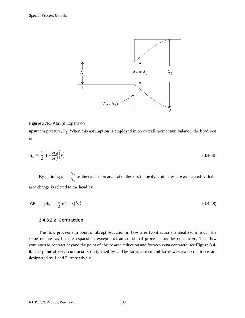
Special Process Models
upstream pressure, P1. When this assumption is employed in an overall momentum balance, the head loss
is
(3.4-38)
By defining as the expansion area ratio, the loss in the dynamic pressure associated with the
area change is related to the head by
(3.4-39)
3.4.3.2.2 Contraction
The flow process at a point of abrupt reduction in flow area (contraction) is idealized in much the
same manner as for the expansion, except that an additional process must be considered. The flow
continues to contract beyond the point of abrupt area reduction and forms a vena contracta, see Figure 3.4-
6. The point of vena contracta is designated by c. The far-upstream and far-downstream conditions are
designated by 1 and 2, respectively.
Figure 3.4-5 Abrupt Expansion
AT = AcA1 A2
1
2
(A2 - A1)
hL12--- 1
A2
A1------–
2
v22=
εA2
A1------=
∆PL ρhL12---ρ 1 ε–( )2v2
2= =
NUREG/CR-5535/Rev 1-Vol I 188

Special Process Models
Consider a sudden contraction in a steady incompressible flow. The loss in dynamic pressure from
the upstream station to the vena contracta is the smaller part of the total loss. Measurements3.4-21 indicate
that the contracting flow experiences a loss no larger than , where
vc is the velocity at the contracta. This loss is at most 24% of the total loss and is neglected in RELAP5.
The dynamic pressure loss associated with the new expansion from the area at the vena contracta to the
downstream area is modeled using the Borda-Carnot assumption with the condition at the vena contracta as
the upstream condition, that is
(3.4-40)
where from continuity considerations for incompressible flow
(3.4-41)
The contraction ratio, , is a function of . This is based on a synthesis of analytical approaches
and generally accepted experimental information.3.4-21 The function in Reference 3.4-21 is in the form of
Figure 3.4-6 Abrupt Contraction
AT Ac A2A1
2
1
c
∆PL 0.04612---ρvc
2
0.12
12---ρv2
2
= =
∆PL12---ρ 1
Ac
A2------–
2
vc2=
vc
A2v2
Ac-----------=
Ac
A2------
A2
A1------
189 NUREG/CR-5535/Rev 1-Vol I
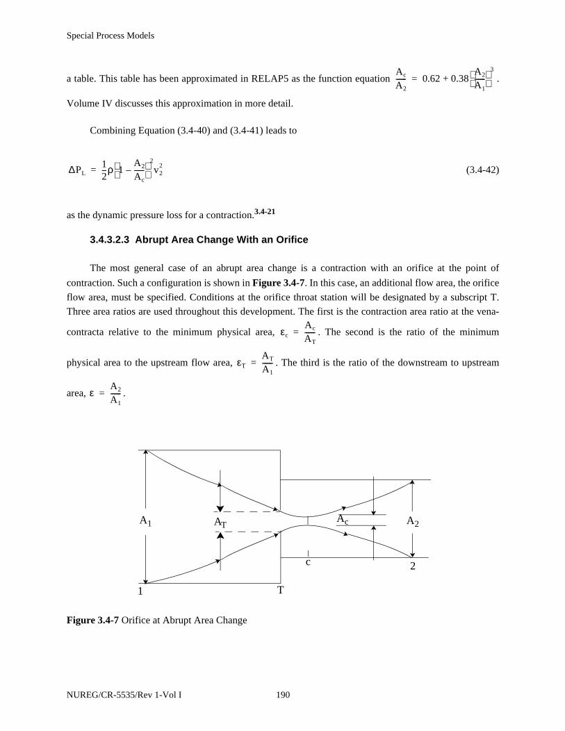
Special Process Models
a table. This table has been approximated in RELAP5 as the function equation .
Volume IV discusses this approximation in more detail.
Combining Equation (3.4-40) and (3.4-41) leads to
(3.4-42)
as the dynamic pressure loss for a contraction.3.4-21
3.4.3.2.3 Abrupt Area Change With an Orifice
The most general case of an abrupt area change is a contraction with an orifice at the point of
contraction. Such a configuration is shown in Figure 3.4-7. In this case, an additional flow area, the orifice
flow area, must be specified. Conditions at the orifice throat station will be designated by a subscript T.
Three area ratios are used throughout this development. The first is the contraction area ratio at the vena-
contracta relative to the minimum physical area, . The second is the ratio of the minimum
physical area to the upstream flow area, . The third is the ratio of the downstream to upstream
area, .
Figure 3.4-7 Orifice at Abrupt Area Change
Ac
A2------ 0.62 0.38
A2
A1------
3
+=
∆PL12---ρ 1
A2
Ac------–
2
v22=
εc
Ac
AT------=
εT
AT
A1------=
εA2
A1------=
A2
2
Ac
c
T1
A1 AT
NUREG/CR-5535/Rev 1-Vol I 190
Special Process Models
The dynamic pressure loss for an abrupt area contraction combined with an orifice is analyzed in a
manner parallel to that for a simple contraction. The loss associated with the contracting fluid stream from
Station 1 to c (the point of vena-contracta) is neglected. The dynamic pressure loss associated with the
expansion from the vena-contracta to the downstream section is given by
(3.4-43)
The contraction ratio, , is a function of . The code uses the same function equation
as is used for a contraction. The function equation is εc = 0.62 + 0.38 (εT)3. Using the continuity equations,
and , Equation (3.4-43) can be written as
(3.4−44)
where Kf = Kg =
Equation (3.4-44) is a generalization applicable to all the cases previously treated. For a pure
expansion, εT = 1, εc = 1, and ε > 1; for a contraction, εT = ε < 1 and εc < 1. Each of these is a special case
of Equation (3.4-44). The two-phase dynamic pressure loss model is based on an adaptation of the general
single-phase head loss given by Equation (3.4-44).
3.4.3.3 Two-Phase Abrupt Area Change Model.
The two-phase flow through an abrupt area change is modeled in a manner very similar to that for
single-phase flow by defining phasic flow areas. The two phases are coupled through the interphase drag, a
common pressure gradient, and the requirement that the phases coexist in the flow passage. As with the
single-phase case, apportioned volume areas are calculated for a one-dimensional branch. This is discussed
in Section 3.5.1.
The one-dimensional phasic stream-tube momentum equations are given in Section 3.1.1. The flow
at points of abrupt area change is assumed to be quasi-steady and incompressible. In addition, the terms in
the momentum equations due to body force, wall friction, and mass transfer are assumed to be small in the
region affected by the area change. The interphase drag terms are retained, since the gradient in relative
velocity can be large at points of abrupt area changes. The interphase drag is increased for co-current
horizontal stratified abrupt area changes in order to ensure more homogeneous flow.
∆PL12---ρ 1
Ac
A2------–
2
vc2=
εc
Ac
AT------= εT
AT
A1------=
vc
ATvT
Ac------------ vT εc⁄= = vT
A2v2
AT-----------
εεT-----v2= =
∆PL12---ρ 1
εεcεT----------–
2
v22=
1ε
εcεT----------=
2
191 NUREG/CR-5535/Rev 1-Vol I

Special Process Models
Equation (3.1-7) and Equation (3.1-8) can be integrated approximately for a steady incompressible,
smoothly varying flow to obtain modified Bernoulli-type equations for each phase
(3.4-45)
and
(3.4-46)
where L1 and L2 are the lengths from the upstream condition to the throat and from the throat to the
downstream condition respectively and where . The term FI is determined from
Equation (3.3-47). The interphase drag is divided into two parts, which are associated with the upstream
and downstream parts of the flow affected by the area change.
3.4.3.4 General Model.
Consider the application of Equation (3.4-45) and (3.4-46) to the flow of a two-phase fluid through a
passage having a generalized abrupt area change. The flow passage is shown in Figure 3.4-8.a Here, the
area AT is the throat or minimum area associated with an orifice located at the point of the abrupt area
change. Since each phase is governed by a modified Bernoulli-type equation, it is reasonable to assume
that losses associated with changes in the phasic flow area can be modeled by separate dynamic pressure
loss terms for both the liquid and gas phases. Hence, it is assumed that the liquid sustains a loss as if it
alone (except for interphase drag) were experiencing an area change from αf1 A1 to αfT AT to αf2 A2; and
the gas phase experiences a loss as if it alone were flowing through an area change from αgl A1 to αgT AT
to αg2 A2. The area changes for each phase are the phasic area changes (see Figure 3.4-8). When the losses
for these respective area changes [based on the Borda-Carnot model and given by Equation (3.4-44)] are
added to Equation (3.4-45) and (3.4-46), the following phasic momentum equations are obtained:
a. In Figure 3.4-8, the flow is shown as a separated flow for clarity. The models developed are equally
applicable to separated and dispersed flow regimes, as evidenced by the calculations performed when the
abrupt area change model was incorporated into RELAP5.3.4-20 The model was verified on single-phase
expansions, contractions, and orifices. Three two-phase problems were also run: (1) expansion case with the
interphase drag equal to zero, which simulates separated flow, (2) expansion case with the interphase drag
appropriate for dispersed flow, and (3) contraction case with the interphase drag appropriate for dispersed
flow.
12---ρfvf
2 P+
1
12---ρfvf
2 P+
2
FI ′
α f------
1
vf1 vg1–( )L1FI′
α f------
2
vf2 vg2–( )L2+ +=
12---ρgvg
2 P+
1
12---ρgvg
2 P+
2
FI ′
α g------
1
vg1 vf1–( )L1FI ′
αg------
2
vg2 v2f–( )L2+ +=
FI ′ α fαgρfρg FI=
NUREG/CR-5535/Rev 1-Vol I 192
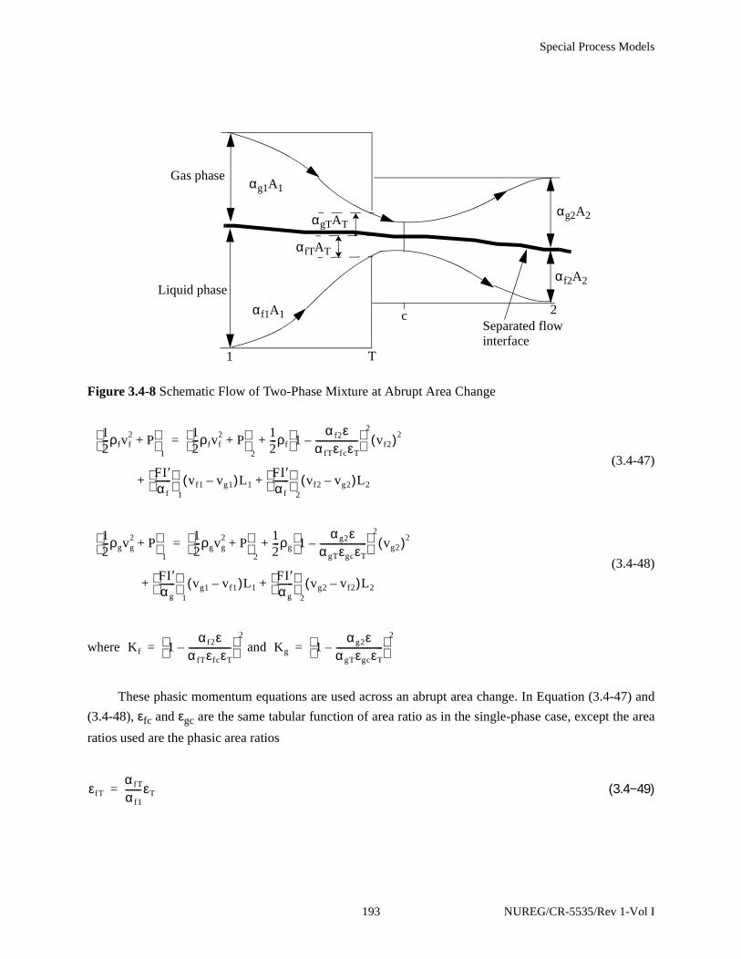
Special Process Models
(3.4-47)
(3.4-48)
where
These phasic momentum equations are used across an abrupt area change. In Equation (3.4-47) and
(3.4-48), εfc and εgc are the same tabular function of area ratio as in the single-phase case, except the area
ratios used are the phasic area ratios
(3.4−49)
Figure 3.4-8 Schematic Flow of Two-Phase Mixture at Abrupt Area Change
Gas phase
T1
c 2αf1A1
αg1A1
αgTAT
αfTAT
αg2A2
αf2A2Liquid phase
Separated flowinterface
12---ρfvf
2 P+
1
12---ρfvf
2 P+
2
12---ρf 1
α f2εα fTεfcεT-------------------–
2
vf2( )2+=
FI ′α f-------
1
vf1 vg1–( )L1FI ′α f-------
2
vf2 vg2–( )L2+ +
12---ρgvg
2 P+
1
12---ρgvg
2 P+
2
12---ρg 1
αg2εαgTεgcεT---------------------–
2
vg2( )2+=
FI ′α g-------
1
vg1 vf1–( )L1FI ′α g-------
2
vg2 vf2–( )L2+ +
Kf 1α f2ε
α fTεfcεT-------------------–
2
and Kg 1αg2ε
αgTεgcεT---------------------–
2
= =
εfT
α fT
α f1-------εT=
193 NUREG/CR-5535/Rev 1-Vol I

Special Process Models
(3.4−50)
respectively. The area ratios, and , are the same as for single-phase flow.
The in Section 3.1.3 momentum Equation (3.1-103) and (3.1-104) are
of the form , where Kg and Kf are defined after
Equation (3.4-47) and (3.4-48).
The interphase drag effects in Equation (3.4-47) and (3.4-48) are important. These terms govern the
amount of slip induced by an abrupt area change; and, if they are omitted, the model will always predict a
slip at the area change appropriate to a completely separated flow situation and give erroneous results for a
dispersed flow.
3.4.3.5 Model Application.
A few remarks concerning the way Equation (3.4-47) and (3.4-48) are applied to expansions and
contractions, both with and without an orifice, are necessary. In a single-phase, steady flow situation and
given the upstream conditions v1 and P1, one can solve for v2 and P2 by using the continuity equation
(v1A1 = v2A2) and Equation (3.4-37). (3.4-47) and (3.4-48), along with the two phasic continuity
equations, can be used in a similar manner except that now the downstream void fraction is an additional
unknown which must be determined.
3.4.3.5.1 Expansion
For the purpose of explanation, consider the case of an expansion (αfT = αf1, αgΤ = αg1, ε > 1, εT = 1,
εfc = εgc = 1, , L1 = 0) for which Equation (3.4-47) and (3.4-48) reduce to
(3.4-51)
(3.4-52)
These two equations with the incompressible continuity equations
αf1vf1A1 = αf2vf2A2 (3.4-53)
εgT
αgT
α g1--------εT=
εA2
A1------= εT
AT
A1------=
HLOSSGjn and HLOSSFj
n
HLOSSGjn 1
2---Kg vg j,
n and HLOSSFjn 1
2---Kf vf j,
n==
FI1′ 0=
12--- ρfvf
2 P+
1
12--- ρfvf
2 P+
2
12--- ρf 1
α f2εα f1
----------–
2
vf2( )2 FI′
α f------
2
vf2 vg2–( )L2+ +=
12--- ρgvg
2 P+
1
12--- ρgvg
2 P+
2
12--- ρg 1
αg2εα g1-----------–
2
vg2( )2 FI ′
α g------
2
vg2 vf2–( )L2+ +=
NUREG/CR-5535/Rev 1-Vol I 194

Special Process Models
and
αg1vg1A1 = αg2vg2A2 (3.4-54)
are a system of four equations having four unknowns, αf2 (αg2 = 1 - αf2), vf2, vg2, and P2, given the
upstream conditions, αf1 (αg1 = 1 - αf1), vf1, vg1, and P1. (The interphase drag, , is a known function of
the flow properties.) It is important to note that the downstream value of the liquid fraction (αf2) is an
additional unknown compared with the single-phase case and is determined (with the downstream
velocities and pressure) by simultaneous solution of Equation (3.4-51) through (3.4-54) without additional
assumptions. It is reassuring that by taking a proper linear combination of Equation (3.4-47) and (3.4-48),
the usual overall momentum balance obtained using the Borda-Carnot3.4-21 assumption can be
obtained.3.4-23,3.4-24
If, as in the cited literature,3.4-23,3.4-24,3.4-25,3.4-26 only the overall momentum balance is used at an
expansion, there will be an insufficient number of equations to determine all the downstream flow
parameters, αf2, vf2, vg2, and P2. The indeterminacy has been overcome in cited works by means of several
different assumptions concerning the downstream void fraction.a In the model developed here [Equation
(3.4-51) and (3.4-52)], division of the overall loss into liquid and gas parts, respectively, results in
sufficient conditions to determine all downstream flow variables, including αf2. In addition, the present
model includes force terms due to interphase drag in Equation (3.4-51) and (3.4-52), which are necessary
to predict the proper amount of slip and void redistribution that occurs at points of area change.
3.4.3.5.2 Contraction
Consider the application of Equation (3.4-47) and (3.4-48) to a contraction. To determine both the
downstream conditions and throat conditions from the upstream values of αf1(αg1), vf1, vg1, and P1, an
additional consideration needs to be made. To obtain the throat values, apply the momentum equations
valid for the contracting section of flow. (Here, the L1 portion of the interphase force is associated with the
contraction.)
(3.4-55)
a. J. G. Collier3.4-23 mentions three different assumptions that have been used: (1) αf2 = αf1, (2) αf2 is given by
a homogeneous model, and (3) αf2 is given by the Hughmark void fraction correlation.
FI ′
12--- ρfvf
2 P+
1
12--- ρfvf
2 P+
T
FI′
α f------
1
vf1 vg1–( )L1+=
195 NUREG/CR-5535/Rev 1-Vol I
Special Process Models
(3.4-56)
αf1vf1A1 = αfTvfTAT (3.4-57)
αg1vg1A1 = αgTvgTAT (3.4-58)
These four equations are solved simultaneously for the values of αfT(αgT), vfT, vgT, and PT at the
throat section (the minimum physical area). No additional or special assumptions are made concerning the
throat conditions, since they follow as a direct consequence of the unique head loss models for each phase.
After the throat values have been obtained, the conditions, at the point of vena-contracta are established,
assuming the void fraction is the same as at the throat. Thus, εfc and εgc are established using the single-
phase contraction function equation and the throat area ratios, εfT and εgT, defined by Equation (3.4-49)
and (3.4-50). The functions are εfc = 0.62 + 0.38(εfT)3 and εgc = 0.62 + 0.38(εgT)3. To determine the
downstream values, Equation (3.4-47) and (3.4-48) can be applied directly from Stations 1 to 2 with the
throat values known, or the expansion loss equations can be used from the throat section to Station 2. Both
approaches produce identical downstream solutions. As in the case of an expansion, because the proper
upstream and downstream interphase drag is included, this modeling approach establishes the phase slip
and resulting void redistribution. An orifice at an abrupt area change is treated exactly as the contraction
explained above (that is, with two separate calculations to establish first the throat and then the
downstream flow variables).
3.4.3.5.3 Countercurrent Flow
The preceding development implicitly assumed a cocurrent flow. For countercurrent flow, Equation
(3.4-47) and (3.4-48) are applied exactly as in cocurrent flow except that the upstream sections for the
respective phases are located on different sides of the abrupt area change. The difference appears in how
the throat and downstream voids are determined. To determine the throat properties, equations similar to
Equation (3.4-55) through (3.4-58) are used with the upstream values appropriate for each phase. These
four equations are then solved for αfT(αgT), vfT, vgT, and PT. To determine the downstream values for each
phase, only the head loss terms are needed for the downstream voids. (The downstream vf, vg, and P do not
appear.) For countercurrent flow, these voids are set such that the downstream void of each phase plus the
upstream void of the opposite phase adds to 1. (Both phases together must fill the flow channel.) With the
throat and downstream voids now known, Equation (3.4-47) and (3.4-48) can be used directly to determine
the total loss for each phase at the abrupt area change.
3.4.4 User-Specified Form Loss
In the calculation of the total form loss, partitioning of the form friction losses between the liquid and
the vapor phases are implemented based on the phasic void fractions. However, there are many practical
12--- ρgvg
2 P+
1
12--- ρgvg
2 P+
T
FI ′
αg------
1
vg1 vf1–( )L1+=
NUREG/CR-5535/Rev 1-Vol I 196
Special Process Models
situations for the users of using flow condition dependent form loss coefficients in order to represent the
friction loss close to experimental values. This section documents the implementation of the general user-
specified form loss coefficients.
The and terms in Section 3.1.3 momentum Equation (3.1-103) andEquation
(3.1-104) contain the user-specified loss term of the form
(3.4-59)
(3.4-60)
where K is either the forward (KF) or reverse (KR) inputted user-specified loss, depending on the phasic
velocity direction.
In many cases the form loss coefficient is a function of the Reynolds number. Thus it is suggested
that the form loss coefficients can be generally expressed as
(3.4-61)
(3.4-62)
where KF and KR are the forward and reverse form loss coefficients; AF, AR, BF, BR, CF, and CR are the
constants that are user-specified and Re is the Reynolds number based on mixture fluid properties. There
are several different ways of defining the mixture Reynolds number based on the way the mixture viscosity
is computed.3.4-27 In RELAP5, the mixture viscosity µm defined by Cicchitti3.4-28 is implemented for
calculating the mixture Reynolds number
µm = X µg + (1 - X) µf (3.4-63)
where µg is the gas viscosity, µf is the liquid viscosity, and X is the static quality.
3.4.5 Crossflow Junction
The RELAP5 numerical scheme is generally formulated using one-dimensional elements. However,
there are several applications where an approximate treatment of crossflow provides an improved physical
HLOSSGjn HLOSSFj
n
HLOSSGjn 1
2---K vg j,
n=
HLOSSFjn 1
2---K vf j,
n=
KF AF BF Re-CF+=
KR AR BR Re-CR+=
197 NUREG/CR-5535/Rev 1-Vol I

Special Process Models
simulation. This is discussed further in Volume II. Three different applications for a crossflow formulation
are described in the following paragraphs.
The first application concerns a small crossflow between two essentially axial flow streams. This
situation is typical of regions such as a reactor core or a steam generator, because the component geometry
provides a large resistance (i.e., small flow rate) to crossflow and a small resistance (i.e., large flow rate) to
axial flow. Hence, simplified crossflow momentum equations can be used to couple a hot flow channel to a
bulk flow channel.
The second application of a crossflow junction is to provide a tee model. In this case, the momentum
flux in the side branch is assumed to be perpendicular to the main stream; thus, the main stream
momentum flux does not contribute to the crossflow momentum formulation.
The third application is modeling of leak flow paths. In this case, the flow is small and governed
primarily by pressure differential, gravity, and flow resistance.
The vapor momentum finite difference equation used in the basic numerical scheme is
(3.4-64)
where
∆xj = (3.4-65)
A parallel equation holds for the liquid phase. It should be noted that the momentum Equation (3.4-
64) is in reality the sum of half the K cell momentum plus half the L cell momentum. This is the reason for
Equation (3.4-65).
In crossflow junctions, just as in the normal junctions, the transverse momentum advection terms are
neglected, i.e., there is no transport of x-direction momentum due to the flow in the transverse direction.
For the case of a small crossflow junction between two axial flow streams (J2 in Figure 3.4-9) all the
geometric input (area, length, elevation change) for both of the volumes relates to the axial flow direction,
as do the wall drag and code-calculated form losses.
αgρg( )jn vg
n 1+ vgn–( )j∆xj
12--- α· gρ· g( )j
nvg
2( )Ln
vg2( )K
n–[ ]∆ t VISCOUS TERMS+ +
α g j,n PL
n 1+ PKn 1+–( )∆t– αgρg( )j
n FWGjn∆xj HLOSSGj
n+( )vg j,n 1+ ∆t–=
αgρg( )jnFIGj
n vg j,n 1+ vf j,
n 1+–( )∆xj∆t– αgρg( )jnBx∆xj∆t+
A+ DDED MASS MASS TRANSFER MOMENTUM+
STRATIFIED PRESSURE GRADIENT EFFECT+
12--- ∆xK ∆xL+( )
NUREG/CR-5535/Rev 1-Vol I 198

Special Process Models
The crossflow area and the length scale can be either user-specified or code-calculated values. When
code-calculated values are used, the volume geometries are defaulted for the case of a cylindrical pipe, and
the appropriate length scale and flow area are used in the code. When user-specified values are used, the
user should provide the representative crossflow area and length scale in the input deck. The length scale
can be calculated as the volume divided by the crossflow area.
Since the connecting K and L volumes are assumed to be predominantly axial flow volumes, the
crossflow junction momentum flux (related to the axial volume velocity in K and L) can be neglected (by
using a junction flag) along with the associated numerical viscous term.
The resulting vapor momentum finite difference equation (when the momentum flux is neglected
using a junction flag) for a crossflow junction between two axial flow streams is
(3.4-66)
A similar equation can be written for the liquid phase. The ∆xj term that is used to estimate the
inertial length associated with crossflow is defined using the diameters of volumes K and L,
(3.4-67)
Figure 3.4-9 Modeling of Crossflows or Leak
J1 J3
V1 V2
J2
J4 J5
X X
αgρg( )jn vg
n 1+ vgn–( )j∆xj αg j,
n PL PK–( )n 1+ ∆t– αgρg( )jnHLOSSGg
nvg j,n 1+ ∆t–=
α gρg( )jnFIGj
n vg j,n 1+ vf j,
n 1+–( )∆xj∆t– αgρg( )jnBx∆xj∆t+
A+ DDED MASS MASS TRANSFER MOMENTUM+
STRATIFIED PRESSURE GRADIENT EFFECT+
∆xj12--- D K( ) D L( )+[ ]=
199 NUREG/CR-5535/Rev 1-Vol I

Special Process Models
if the default is used. If user-specified lengths are input, they are used instead of D(K) and D(L).
The crossflow option can be used with the crossflow junction perpendicular to the axial flow in
volume L (or K) but parallel to the axial flow in volume K (or L) (see Figure 3.4-10). Here, the situation
regarding the half cell momentum contribution in volume L is the same as described above. The half cell
momentum contribution associated with volume K is the same as for a normal junction. This type of
crossflow modeling can be used for a 90-degree tee simulation.
The resulting vapor momentum finite difference equation for a crossflow junction perpendicular to
the axial flow in volume L but parallel to the axial flow in volume K is
(3.4-68)
where the momentum flux in volume L is neglected by using a junction flag.
A similar equation can be written for the liquid phase. The ∆xj term has the form
Figure 3.4-10 Simplified Tee Crossflow
K
L VL
J2J1
J3X
α gρg( )jn vg
n 1+ vgn–( )j∆xj
12--- α· gρ· g( )j
nvg
2( )– Kn[ ]∆ t VISCOUS TERM( )K+ +
αg j,n PL
n 1+ PKn 1+–( )∆t– αgρg( )j
n FWGjn∆xj HLOSSGj
n+[ ] vg j,n 1+ ∆t–=
α gρg( )jnFIGj
n vg j,n 1+ vf j,
n 1+–( )∆xj∆t– αgρg( )jnBx∆xj∆t+
A+ DDED MASS MASS TRANSFER MOMENTUM+
STRATIFIED PRESSURE GRADIENT EFFECT+
NUREG/CR-5535/Rev 1-Vol I 200

Special Process Models
(3.4-69)
if the default is used. If a user-specified length is input for the L volume, it is used instead of D(L).
For leak flows and minor flow paths, the modeling approach shown in Figure 3.4-11 is
recommended. Here, J3 is the normal flow path, whereas junction J1, volume M, and junction J2 represent
the leak flow path. Junctions J1 and J2 should be modeled as tee junctions described above. The only
reason for using volume M is to obtain a correct representation of the gravity head from K to L. If a
crossflow junction were modeled directly between volumes K and L, then there would be no gravity head
in the leak flow junction equation. Leak paths may also be modeled using a crossflow junction that is
perpendicular to both the K and L volumes when the leak flow is between volumes having the same
volume center elevation.
3.4.6 Water Packing Mitigation Scheme
Large pressure spikes that cannot be explained by known physical phenomena are at times
encountered when Eulerian-type computer codes are used to analyze integral systems tests or reactor
accidents. These fictitious pressure spikes are sometimes calculated when steam is disappearing from, and
water is about to fill, a control volume. The situation is often referred to as water packing.
The cause of the anomalous pressure spikes is the discontinuous change in compressibility between a
two-phase mixture of small void fraction and a pure liquid phase, and approximations inherent in the
discrete momentum equations. The same problems are seen using a two-fluid model or the homogeneous
equilibrium model. Consider the homogeneous equilibrium case and a cell that is nearly full of liquid with
a net influx of mass. The density-pressure relationship used to calculate the new time pressure is based
Figure 3.4-11 Leak Flow Modeling
∆xj12--- ∆xK D L( )+[ ]=
X
X K
L
M
J2
J1
J3
201 NUREG/CR-5535/Rev 1-Vol I

Special Process Models
upon the beginning of time step values for the state properties and derivatives. The compressibility of this
low void fraction cell is dominated by the mass transfer. The equivalent mixture corresponds to a highly
compressible fluid, i.e., significant volume changes can easily occur with very little change in pressure.
This high compressibility can allow significant continuing influx of liquid with very little pressure rise. In
fact, in some cases the net volume influx of liquid during the time step can be larger than the initial vapor
volume in the cell. This filling of the cell is accompanied by only slight pressure changes. This small
change in pressure may do little to slow down or reverse the liquid influx momentum. If this is the case, the
following time step will be taken with a liquid full cell and large liquid influx momentum existing at the
beginning of the time step. Because the liquid is nearly incompressible, this large influx of liquid
momentum will cause a large increase in pressure during this following time step.
In the neighborhood of these spurious numerical pressure spikes, the calculated phasic velocities may
increase substantially, and smaller time-step sizes are needed to satisfy the material Courant stability limit.
Thus, the computational efficiency is greatly reduced by the presence of water packing. Of course, the
computed pressure spikes are unphysical. Furthermore, water packing may severely distort the transient
solution by changing the void distribution or driving the liquid completely out of an open system.
A water packing scheme has been installed to mitigate these spikes. The water packing scheme
closely follows the method used in the TRAC code.3.4-29,3.4-30 It involves a detection scheme to determine
when a pressure change occurs in a volume containing mostly liquid. It then imposes changes to the
momentum equations, followed by a recalculation of the pressure solution using the sparse matrix solver.
The detection logic used in the water packing scheme evolved from experience gained in running a
vertical fill problem.3.4-31 The detection logic requires the following formula for the pressure:
(3.4-70)
where volume K is the volume that water packs and volume L is the next volume (see Figure 3.4-12). In
volume K, the detection scheme also requires a void fraction (αg) < 0.12, the liquid temperature (Tf) to be
less than the saturation temperature (Ts), the volume to be flagged as vertically stratified, and the next
volume above to be highly voided. Thus, a legitimate water hammer situation would not be eliminated by
the water packing scheme.
The next part of the scheme involves altering the liquid momentum equation so that only small
pressure changes will occur when the volume fills with water. The scheme involves modifying the
coefficient that multiplies the pressure change in the filling volume. The modification multiplies this
coefficient by a large number and is discussed in more detail in the next paragraph. Since the pressure
solution is rejected when water packing occurs, the pressure calculation is repeated using the sparse matrix
solver.
The finite difference form of the liquid momentum equation used can be written
PKn 1+ PK
n 0.0023PKn+≥
NUREG/CR-5535/Rev 1-Vol I 202
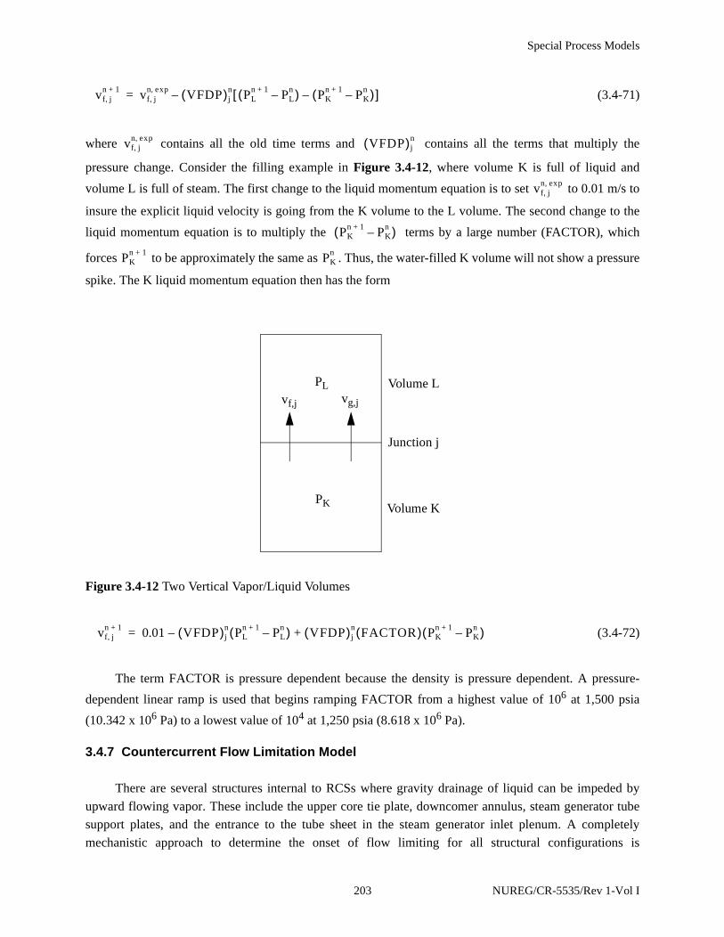
Special Process Models
(3.4-71)
where contains all the old time terms and contains all the terms that multiply the
pressure change. Consider the filling example in Figure 3.4-12, where volume K is full of liquid and
volume L is full of steam. The first change to the liquid momentum equation is to set to 0.01 m/s to
insure the explicit liquid velocity is going from the K volume to the L volume. The second change to the
liquid momentum equation is to multiply the terms by a large number (FACTOR), which
forces to be approximately the same as . Thus, the water-filled K volume will not show a pressure
spike. The K liquid momentum equation then has the form
(3.4-72)
The term FACTOR is pressure dependent because the density is pressure dependent. A pressure-
dependent linear ramp is used that begins ramping FACTOR from a highest value of 106 at 1,500 psia
(10.342 x 10⁶ Pa) to a lowest value of 104 at 1,250 psia (8.618 x 10⁶ Pa).
3.4.7 Countercurrent Flow Limitation Model
There are several structures internal to RCSs where gravity drainage of liquid can be impeded by
upward flowing vapor. These include the upper core tie plate, downcomer annulus, steam generator tube
support plates, and the entrance to the tube sheet in the steam generator inlet plenum. A completely
mechanistic approach to determine the onset of flow limiting for all structural configurations is
Figure 3.4-12 Two Vertical Vapor/Liquid Volumes
vf j,n 1+ vf j,
n exp, VFDP( )jn PL
n 1+ PLn–( ) PK
n 1+ PKn–( )–[ ]–=
vf j,n exp, VFDP( )j
n
vf j,n exp,
PKn 1+ PK
n–( )
PKn 1+ PK
n
PLvg,jvf,j
PK
Volume L
Junction j
Volume K
vf j,n 1+ 0.01 VFDP( )j
n PLn 1+ PL
n–( )– VFDP( )jn FACTOR( ) PK
n 1+ PKn–( )+=
203 NUREG/CR-5535/Rev 1-Vol I
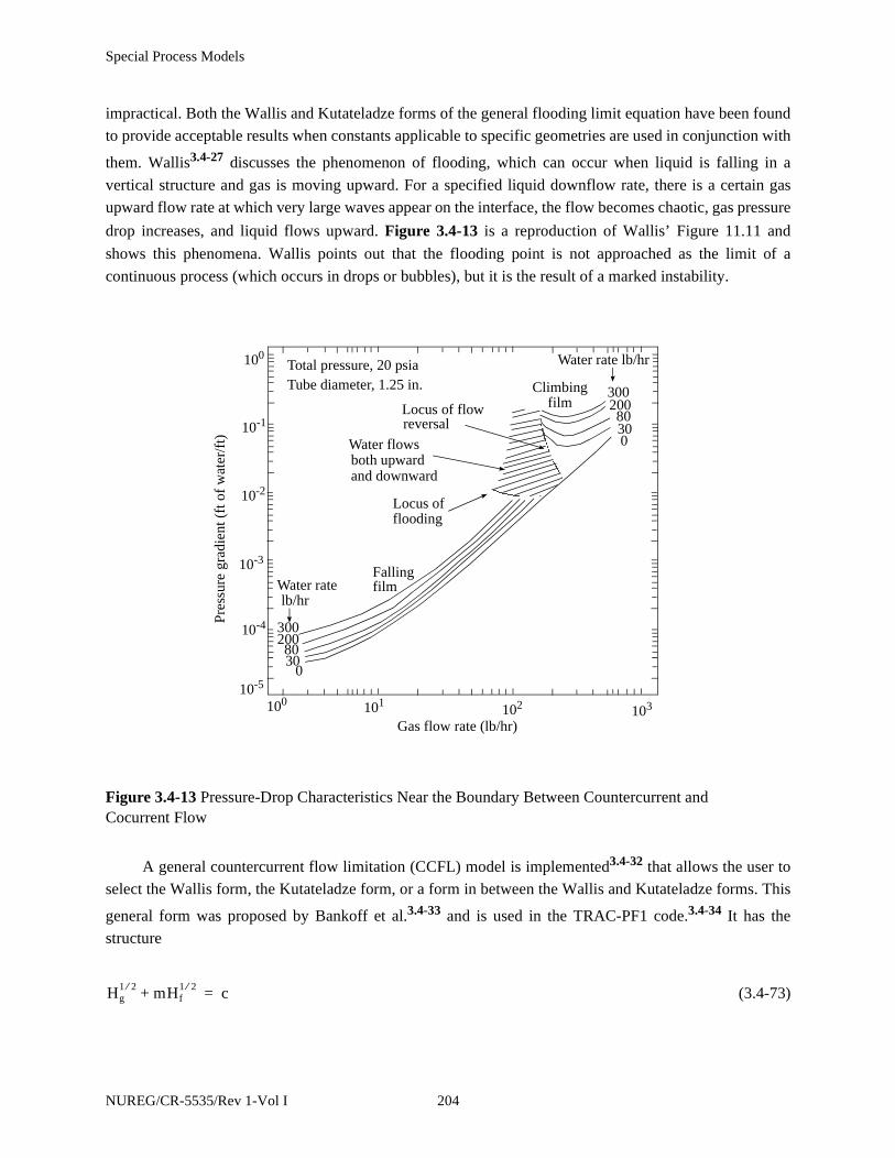
Special Process Models
impractical. Both the Wallis and Kutateladze forms of the general flooding limit equation have been found
to provide acceptable results when constants applicable to specific geometries are used in conjunction with
them. Wallis3.4-27 discusses the phenomenon of flooding, which can occur when liquid is falling in a
vertical structure and gas is moving upward. For a specified liquid downflow rate, there is a certain gas
upward flow rate at which very large waves appear on the interface, the flow becomes chaotic, gas pressure
drop increases, and liquid flows upward. Figure 3.4-13 is a reproduction of Wallis’ Figure 11.11 and
shows this phenomena. Wallis points out that the flooding point is not approached as the limit of a
continuous process (which occurs in drops or bubbles), but it is the result of a marked instability.
A general countercurrent flow limitation (CCFL) model is implemented3.4-32 that allows the user to
select the Wallis form, the Kutateladze form, or a form in between the Wallis and Kutateladze forms. This
general form was proposed by Bankoff et al.3.4-33 and is used in the TRAC-PF1 code.3.4-34 It has the
structure
(3.4-73)
Figure 3.4-13 Pressure-Drop Characteristics Near the Boundary Between Countercurrent and Cocurrent Flow
030
30020080
Climbingfilm
Water rate
Water rate lb/hr
Locus of flowreversal
Water flowsboth upwardand downward
Locus offlooding
Fallingfilm
lb/hr
030
30020080
Total pressure, 20 psiaTube diameter, 1.25 in.
100 101103102
10-5
10-4
10-3
10-2
10-1
100
Gas flow rate (lb/hr)
Pres
sure
gra
dien
t (ft
of
wat
er/f
t)
Hg1 2⁄ mHf
1 2⁄+ c=
NUREG/CR-5535/Rev 1-Vol I 204
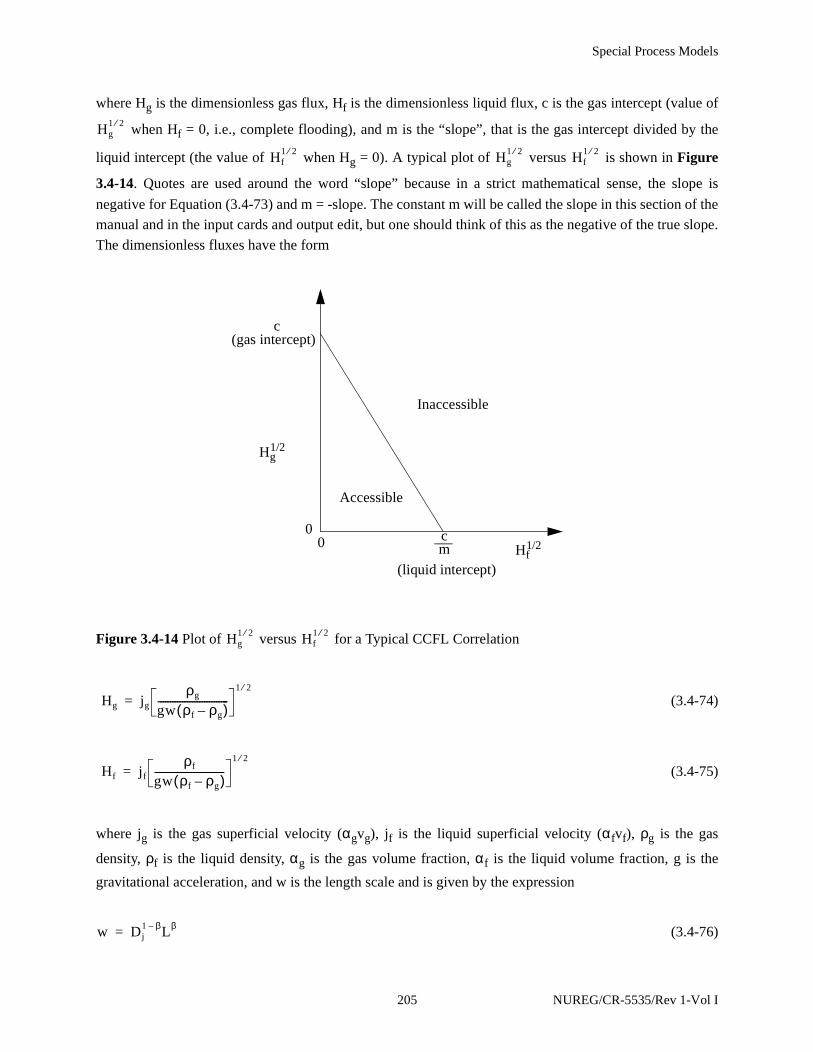
Special Process Models
where Hg is the dimensionless gas flux, Hf is the dimensionless liquid flux, c is the gas intercept (value of
when Hf = 0, i.e., complete flooding), and m is the “slope”, that is the gas intercept divided by the
liquid intercept (the value of when Hg = 0). A typical plot of versus is shown in Figure
3.4-14. Quotes are used around the word “slope” because in a strict mathematical sense, the slope is
negative for Equation (3.4-73) and m = -slope. The constant m will be called the slope in this section of the
manual and in the input cards and output edit, but one should think of this as the negative of the true slope.
The dimensionless fluxes have the form
(3.4-74)
(3.4-75)
where jg is the gas superficial velocity (αgvg), jf is the liquid superficial velocity (αfvf), ρg is the gas
density, ρf is the liquid density, αg is the gas volume fraction, αf is the liquid volume fraction, g is the
gravitational acceleration, and w is the length scale and is given by the expression
(3.4-76)
Figure 3.4-14 Plot of versus for a Typical CCFL Correlation
Hg1 2⁄
Hf1 2⁄ Hg
1 2⁄ Hf1 2⁄
0 cm
Inaccessible
(gas intercept)c
Hg 1/2
0
Hf1/2
Accessible
(liquid intercept)
Hg1 2⁄ Hf
1 2⁄
Hg jg
ρg
gw ρf ρg–( )-----------------------------
1 2⁄=
Hf jf
ρf
gw ρf ρg–( )-----------------------------
1 2⁄=
w Dj1 β– Lβ=
205 NUREG/CR-5535/Rev 1-Vol I
Special Process Models
where β is a user-input constant.
In Equation (3.4-76), Dj is the junction hydraulic diameter and L is the Laplace capillary constant,
given by
(3.4-77)
In Equation (3.4-76), β can be a number from 0 to 1. For β = 0, the Wallis form of the CCFL equation
is obtained; and for β = 1, the Kutateladze form of the CCFL equation is obtained. For 0 < β < 1, a form in
between the Wallis and Kutateladze forms is obtained; and Bankoff3.4-33 suggests that β be correlated to
data for the particular geometry of interest. He has included a possible function for β, although it is
somewhat restrictive. The form of Equation (3.4-73) through (3.4-77) is general enough to allow the
Wallis or Kutateladze form to appear at either small or large diameters. Other approaches (e.g., Tien, et.
al.3.4-35) appear to be more restrictive by defaulting to the Wallis form at small diameters and the
Kutateladze form at large diameters.
With regard to the solution method, if the CCFL model is requested by the user, the coding checks if
countercurrent flow exists and if the liquid downflow exceeds the limit imposed by Equation (3.4-73). If
this is true, the sum momentum equation [Equation (3.1-103)] and the flooding limit equation are applied.
This approach was suggested by Trapp,a who observed that the CCFL model is similar to the choking
model in that both place limits on the momentum equations. He observed that since the flooding
phenomenon can be incorporated by altering the interphase friction (as is done in TRAC-PF1), it can also
be incorporated by replacing the code’s difference momentum equation [Equation (3.1-104)] with the
flooding limit equation. The difference equation contains the interphase friction, whereas the sum equation
does not. (In the choking model, the sum momentum equation is replaced with the choking limit equation.)
This method is advantageous in that the phasic velocities still must satisfy the sum momentum equation,
which contains gravity and pressure terms. The numerical form of Equation (3.4-73) needed by the code is
obtained by letting and , solving for , and squaring the equation, which results in
(3.4-78)
Linearization of gives
a. Personal communication, J. A. Trapp, January 1987.
Lσ
g ρf ρg–( )------------------------
1 2⁄=
cg
Hg
vg------= cf
Hf
vf-----= mHf
1 2⁄
m2cf j,n vf j,
n 1+ c2 2c cg j,n( )1 2⁄
vg j,n 1+( )1 2⁄
– cg j,n vg j,
n 1++=
vg j,n 1+( )1 2⁄
NUREG/CR-5535/Rev 1-Vol I 206

Special Process Models
(3.4-79)
and substitution into Equation (3.4-78) gives
(3.4-80)
3.4.8 Mixture Level Tracking Model
Accurate tracking of liquid levels is essential for modeling gravity-driven cooling systems. In
modeling a reactor system using RELAP5, a set of large hydrodynamic volumes are used to model the
various components. Because the discretization of the governing equations uses mean void fractions in
each control volume, a fine nodalization is required to resolve a large change in void fraction, such as is
associated with a liquid level. Even that may not be adequate to model the phenomena because RELAP5
uses a highly diffusive upwind difference scheme to discretize the advection terms. To compensate for the
inherent limitation of the finite-difference scheme used in RELAP5 and to allow a coarser nodalization to
reduce the computational cost, a mixture level tracking model is implemented in RELAP5/MOD3.
The mixture level tracking model is intended to model situations in which the void fraction increases
in the vertical direction. In places where there is a flow restriction such as a grid spacer or tie plate in a rod
bundle, liquid may pool on the flow restriction leading to an inverted flow profile (void fraction decreasing
in the vertical direction) and multiple mixture levels may appear. An inverted void profile may also appear
when steam is injected below the surface of a subcooled pool and the vapor condenses as it rises due to
buoyancy. To handle multiple mixture levels and inverted void profiles, RELAP5/MOD3 divides the
vertical flow passages in the user input into “level stacks” of volumes and allows only one mixture level
per level stack. Level stacks are built during the input processing phase of a computation. They are defined
as a set of volume singly connected in the vertical direction containing no flow restrictions between the
volumes. Junctions which have been input as “abrupt” constitute flow restrictions for the purposes of the
mixture level tracking model. The level tracking model ignores multiple junctions connected to the sides of
volumes for the purpose of building level stacks. The code searches for the head of a level stack by moving
from volume to volume to find a volume which has no vertical junction on its top face, or has an abrupt
junction attached to it top face, or is attached to a volume through the junction attached to its top face in
which the mixture level model has been deactivated by user input. If a volume has multiple junctions
attached to its top or bottom faces, it is treated as if the user had deactivated the level tracking model in the
volume. Multiple vertical connections on the top or bottom faces of a volume is not allowed by the mixture
level tracking model because the level appearance logic examines the void distribution over three adjacent
volumes to determine whether a void discontinuity exists. If there is more than one volume “above” or
“below” the current volume, the model has no way to determine whether a void discontinuity exists
because it has no way of determining which volume is “above” or “below”. The code searches for a
mixture level beginning at the head of a level stack and continuing down until a mixture level is found or
the bottom of the stack is found. Once a level has been found in a stack, the level is propagated from
vg j,n 1+( )1 2⁄
vg j,n( )1 2⁄ 1
2--- vg j,
n( ) 1 2⁄–vg j,
n 1+ vg j,n–( )+=
m2cf j,n vf j,
n 1+ c cg j,n( )1 2⁄
vg j,n( ) 1 2⁄–
cg j,n–[ ] vg j,
n 1++ c2 c cg j,n( )1 2⁄
vg j,n( )1 2⁄
–=
207 NUREG/CR-5535/Rev 1-Vol I
Special Process Models
volume to volume within the stack as fluid conditions dictate and another level cannot be initiated in the
stack until the original mixture level disappears from the stack. A mixture level can disappear only by
propagation out of the top or bottom of the stack. If a level stack contains no mixture level, it is searched
from the top down each time advancement until a mixture level is initiated in the stack and then the level is
propagated as described above. The stack is searched from the top down so that the mixture level, if found,
is placed as high in the stack as possible.
The mixture level tracking model implemented in RELAP5/MOD3 is based on TRAC-BF1/
MOD1.3.4-36,3.4-37 The mixture level is defined as the location where a sharp change of the void fraction
distribution exists. This sharp change is associated with the change in flow regime. The model consists of
five parts.
1. Detection of the mixture level appearance.
2. Calculation of mixture level parameters that are necessary to describe a mixture level,such as the position and velocity of the level, and the void fractions above and belowthe level.
3. Movement of the mixture level from volume to volume.
4. Modification of the mass and energy equations of RELAP5 to accurately convect voidfractions above and below the mixture level, and modification of the density terms,the pressure gradient, and the momentum flux terms in the momentum equationaccording to the location of the mixture level.
5. Modification of the heat transfer calculation according to the mixture level.
The details of the model and its implementation in RELAP5 are presented in the next subsections.
3.4.8.1 Detection of Level Appearance.
The mixture level is the location of an abrupt change in void fraction that is associated with a change
in flow regime. There are two types of mixture levels, normal and inverted. With a normal mixture level
(void profile), the void fraction increases in the upward axial direction, while with an inverted void profile,
the void fraction decreases in the upward axial direction. These situations are illustrated in Figure 3.4-15,
Figure 3.4-16, and Figure 3.4-17. Two situations that give rise to a normal void profile are heating along a
vertical flow path and depressurization in a vertical column. Inverted void profiles typically arise as the
result of liquid pooling in the upper and lower tie plates of a BWR pressure vessel. If more than one
junction is connected to the top or if more than one junction is connected to the bottom, the mixture level
model is not used and is turned off.
NUREG/CR-5535/Rev 1-Vol I 208

Special Process Models
Figure 3.4-15 Mixture Level in Normal Void Profile
Figure 3.4-16 Mixture Level in a Volume Below a Void Fraction Inversion
j+1
j
α-
αK
αM
dzL
dzlL
α+L
L
α+
j+1
j
dzL
dzlL α-
αK
αM
L
L
209 NUREG/CR-5535/Rev 1-Vol I

Special Process Models
The logic for the detection of a mixture level appearance in a computational cell is based on BWR
experimental data and numerical experiments.3.4-37,3.4-40,3.4-41 The logic for detecting a mixture level is
different for the two different kinds of mixture levels.
The level detection logic for a normal void profile, Figure 3.4-15, is
αM - αL > δαc (default = 0.2) (3.4-81)
or
αL- αK > δαc (default = 0.2) (3.4-82)
and
αM > αc (default = 0.7) (3.4-83)
Here, αc is the minimum allowable void fraction in the cell above a normal mixture level, and δαc is
the smallest change that signals the presence of a normal mixture level. The values in parentheses are the
default values used in RELAP5/MOD3 and are recommended by Cheung et al.3.4-40 The notation α or αg
is used for volume vapor fraction (void fraction). The notation αf is used for volume liquid fraction.
Figure 3.4-17 Mixture Level Above a Void Fraction Inversion
αM
α+
α-
αK
dzL
j+1
j
L
LdzlL
NUREG/CR-5535/Rev 1-Vol I 210
Special Process Models
The logic for an inverted void profile depends on whether a particular cell is above or below a void
inversion. A mixture level is defined as being below a void profile inversion Figure 3.4-16 if
αL - αM > δαj (default = 0.1) (3.4-84)
If a mixture level is above a void profile inversion (Figure 3.4-17), the criteria becomes
αK - αL > δαj (default = 0.1) (3.4-85)
The void inversion logic is activated if there is an orifice at the junction. The level detection logic is
summarized in block diagrams as shown in Figure 3.4-18, Figure 3.4-19, Figure 3.4-20, and Figure 3.4-
21.
3.4.8.2 Calculation of Level Parameters.
The parameters that describe the mixture level are:
1. The void fraction above and below the level
2. The location of the level (dzl)
3. The mixture level velocity (vlev)
3.4.8.2.1 Determination of the Void Fraction Above and Below the Level
The correlations to calculate the void fraction above and below the level , respectively,
are given below for the three cases:
1. Normal profile
2. Void inversion above volume L or flow restriction at the top of volume L
3. Void inversion below volume L or flow restriction at the bottom of volume L
Case 1: Normal Void Profile
For a normal void profile, the void fraction below the level is assumed to equal the void fraction in
volume K:
(3.4-86)
αL+ and αL
-
αL+ and αL
-
αL- = αK
211 NUREG/CR-5535/Rev 1-Vol I

Special Process Models
Figure 3.4-18 Level Detection Logic Diagram
condition for volume L
Determine void profile
Is
flow restriction at bottom of volume L
Yes A
Yes A
Is
αK - αL > δαj
?
?
Is
flow restriction at top of volume L
YesB
YesB
Is
αL- αM > δαj
?
?
C
Volume L is above avoid profile inversion
Volume L is below a void profile inversion
Volume L is within a
normal void profile
No
No
No
No
NUREG/CR-5535/Rev 1-Vol I 212
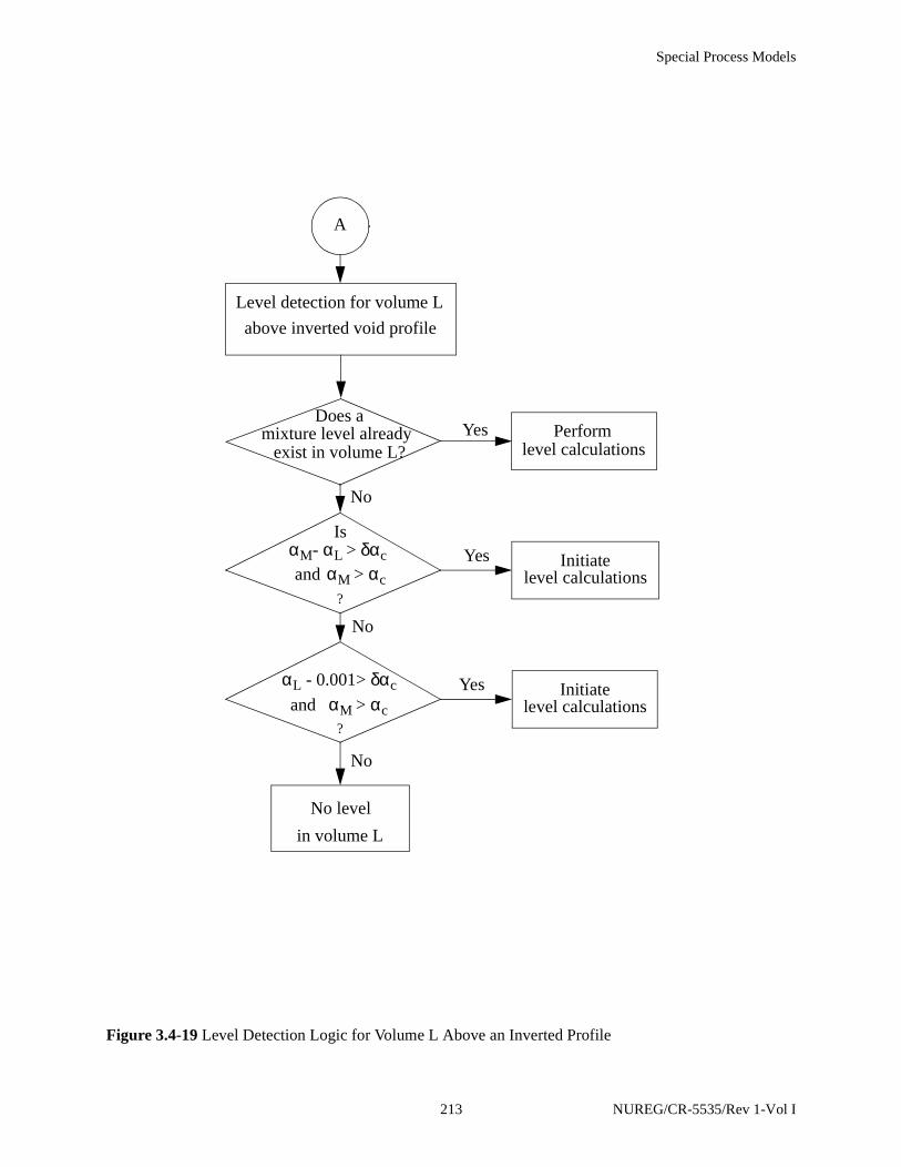
Special Process Models
Figure 3.4-19 Level Detection Logic for Volume L Above an Inverted Profile
A
Level detection for volume L
above inverted void profile
Does a mixture level already Yes Perform
level calculations
αM- αL > δαc
exist in volume L?
Is
αM > αc
αM > αc
αL - 0.001> δαc
?
Initiatelevel calculations
Initiatelevel calculations
No level
in volume L
Yes
Yes
and
and
?
No
No
No
213 NUREG/CR-5535/Rev 1-Vol I
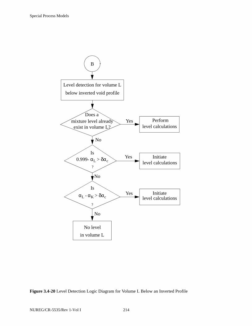
Special Process Models
Figure 3.4-20 Level Detection Logic Diagram for Volume L Below an Inverted Profile
B
Level detection for volume L
below inverted void profile
Does a mixture level already Yes Perform
level calculations
0.999- αL > δαc
exist in volume L?
Is
?
αL - αK > δαc
?
Initiatelevel calculations
Initiatelevel calculations
No level
in volume L
Is
Yes
Yes
No
No
No
NUREG/CR-5535/Rev 1-Vol I 214
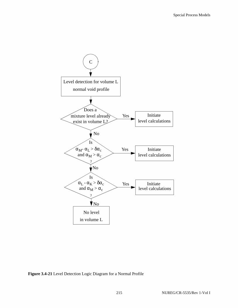
Special Process Models
Figure 3.4-21 Level Detection Logic Diagram for a Normal Profile
C
Level detection for volume L
normal void profile
Does a mixture level already Yes Initiate
level calculations
αM- αL > δαc
exist in volume L?
Is
and αM > αc
αL - αK > δαc
Initiatelevel calculations
Initiatelevel calculations
No level
in volume L
Is
Yes
Yes
No
No
No
?
and αM > αc
?
215 NUREG/CR-5535/Rev 1-Vol I

Special Process Models
In the absence of entrainment of liquid from below the level, the void fraction above the level is
given by:
(3.4-87)
If the velocity at the cell junction is upward, the void fraction is derived from the correlation of
the entrainment liquid mass flux (Glent) developed by Rosen3.4-42 as
(3.4-88)
and
(3.4-89)
where
vf,j+1 = the junction liquid velocity
Aj+1 = the junction area
AL = the average area of the control volume
The entrainment liquid mass flux (Glent) is expressed by
(3.4-90)
where
CK = (3.4-91)
VCRIT = (3.4-92)
αL+ = αM
αL+
αL+ 1
Glent
ρfvf-----------–=
vf vf j 1+,Aj 1+
AL-----------
=
Glent 3.0x10 5– CK0.5 530 CK2.1•+( )ρf ρg–
ρg----------------
0.5
jgρg=
2.0 DMAX jg••
VCRIT gσ
ρf ρg–----------------
0.5
••------------------------------------------------------------------
2.0σg ρf ρg–( )
ρg2
----------------------------0.25
NUREG/CR-5535/Rev 1-Vol I 216
Special Process Models
DMAX = (3.4-93)
In the above expression, Glent is calculated using donor cell-averaged values for ρf, ρg, and σ at cell
L. The value of jg is set equal to (for positive vf)
jg = αM vg (3.4-94)
where
(3.4-95)
and vg,j+1 is the junction vapor phasic velocity.
If either vf,j+1 or vg,j+1 is negative, is given by
(3.4-96)
Case 2: Void Inversion Above Volume L or Flow Restriction at the Top of Volume L
The calculation of the void fraction above and below the level ( and ) is similar to Case 1
except with the following modification.
The volumetric vapor flux used in Equation (3.4-90) and (3.4-91) becomes
jg = 0.999vg (3.4-97)
If vg.j+1 is negative, then
(3.4-98)
Case 3: Void Inversion Below Volume L or Flow Restriction at the Bottom of Volume L
For a cell mixture level occurring above a void fraction inversion or bottom cell area reduction, the
void fraction below the level is calculated using the drift flux approximation
0.3375ρgvg
2
g ρf ρg–( )------------------------
vg vg j 1+,Aj 1+
AL-----------
=
αL+
αL+ αM=
αL+ αL
-
αL+ 0.999=
αL –
217 NUREG/CR-5535/Rev 1-Vol I

Special Process Models
(3.4-99)
where
vgj = (3.4-100)
Co = (3.4-101)
C∞ = (3.4-102)
Rouhani’s3.4-43 correlation is used for C∞. The parameters used in calculating C∞ are based on cell-
centered quantities. The volumetric fluxes and are calculated using junction-donored velocities from
bottom cell j and void fractions of either αK or , depending on whether or not the phasic velocities are
positive or negative, respectively.
(3.4-103)
(3.4-104)
(3.4-105)
where
(3.4-106)
(3.4-107)
αL- jg
-
Coj- vgj+-----------------------=
1.41σg ρf ρg–( )
ρf2
----------------------------
14---
C∞ C∞ 1–ρg
ρf-----–
1.0 0.2ρf gDh( )
12---
αgρgvg α fρfvf+--------------------------------------------
12---
+
jg- jf
-
αL-
jg- 1
2---vg j,
′ α g K, αL- +( ) vg j,
′( ) α g K, αL-–( )sgn+[ ]=
jf- 1
2---vf j,
′ α f K, 1 α– L- ( )+[ ] vf j,
′( ) α f K, 1 αL-–( )–[ ]sgn+{ }=
j- jf- jg
- +=
vf j,′ vf j,
Aj
AL------
=
vg j,′ vg j,
Aj
AL------
=
NUREG/CR-5535/Rev 1-Vol I 218
Special Process Models
The logic and correlations used to calculate are the same as for the normal void profile scheme.
3.4.8.2.2 Location of the Mixture Level
Once the presence of a level is determined in a particular volume, a level flag is set and the level
parameters are calculated. The position of the level (dzlL) of a cell with length dzL is given by
(3.4-108)
where the above and below mixture level void fractions are given above.
3.4.8.2.3 Velocity of Level Movement
The level velocity vlev is obtained by forming a difference approximation to the time derivative of
Equation (3.4-108) as
(3.4-109)
3.4.8.3 Movement of Mixture Level Between Volumes.
Once the position and velocity of a mixture level has been determined, its position at the end of the
time advancement is estimated. If the mixture is predicted to lie outside of the volume in which it currently
resides, the level is moved into the appropriate volume before the advancement is attempted. This is done
to prevent pressure spikes and oscillations which would result from the discontinuous change in the flow
regime in the junction through which the mixture level passes when moving from one volume to an
adjacent volume. The algorithm for the movement of the mixture level from one volume into an adjacent
volume is based on the level crossing algorithm developed at The Pennsylvania State University for the
TRAC-BWR code.3.4-38,3.4-39
The level crossing algorithm consists of three parts:
1. Prediction of the position of the mixture level at the end of the advancement
2. Determination of the mixture level parameters in its new location
3. Computation of the phasic velocities in the junction through which the mixture levelpassed when moving from one volume to an adjacent volume
αL+
dzlL dzL
αL+ αL–
αL+ αL
- –-------------------
=
vlev
dzL
dαL
dt--------- dzlL
dαL+
dt---------– dzL dzlL–( )
dαL-
dt---------–
αL+ αL
-–--------------------------------------------------------------------------------------------=
219 NUREG/CR-5535/Rev 1-Vol I
Special Process Models
3.4.8.3.1 Prediction of Mixture Level Position
The prediction of the position of the mixture level is accomplished by a simple level velocity
extrapolation as shown in Equation (3.4-110):
(3.4-110)
If the projected level position is negative, the mixture level is moved into the volume below the
current volume if the volume below the current volume is within the same level stack or the volume below
the current volume is the head of an adjacent level stack and no level exists in the adjacent level stack. If
the projected level position is greater than the height of the current volume, the mixture level is moved into
the volume above the current volume if the volume above the current volume lies in the same level stack or
if the volume above the current volume is the bottom volume of an adjacent level stack and there is no
mixture level in the adjacent level stack.
3.4.8.3.2 Determination of Level Parameters in New Location
Once the level has been determined to reside in a different volume from the current volume, the level
parameters in the two volumes must be reset to reflect the new location. The level parameters which must
be computed for its new location are the location of the level within its new volume, the above and below
level void fractions, and the velocity of the mixture level in the new volume. The location of the level in
the new volume is set to either the top or bottom of the volume depending upon whether the level enters
the volume from above or below. The void fraction in the volume containing the mixture level is adjusted
so that there is enough of the minor phase (the minor phase is vapor if the mixture level lies at the top of
the volume and the minor phase is liquid if the mixture level lies at the bottom of the volume) to support
the presence of a mixture level. Finally the above and below level void fractions are determined. The
equations used for these adjustments are shown below for the situation in which the mixture level moves
down from volume L into volume K (See Figure 3.4-15):
(3.4-111)
(3.4-112)
(3.4-113)
dzljn 1+ dzlj
n vlev,jn dtn•+=
dzlKn dzK=
vlev,Kn vlev,L
n=
αKn αK
n εα+=
αLn αL
n VK ρf ρg–( )K
VL ρf ρg–( )L
-------------------------------εα–=
if αKn εα<
NUREG/CR-5535/Rev 1-Vol I 220

Special Process Models
(3.4-114)
3.4.8.3.3 Phase Velocity Adjustment
After the level parameters are determined for the new location of the level, the phase velocities in the
junction connecting the two volumes must be recomputed. This is needed because the flow regime in the
junction depends upon the mixture level location. If the mixture level is in the volume at the top of the
junction (top with respect to gravity), the flow regime in the junction is the low void fraction bubbly flow
regime and if the mixture level is in the volume at the bottom of the junction, the flow regime is the high
void annular/mist or mist flow regime. The magnitude of the interfacial friction is very different in these
two flow regimes which results in a different relative velocity between the phases and a different slip ratio.
If the phase velocities were not recomputed to be consistent with the new flow regime in the junction,
pressure spikes and oscillations would result as the phase velocities adjusted to the new flow regime. The
velocity of the major phase in the junction, i.e. the vapor velocity in annular/mist or mist flow and the
liquid velocity in bubbly flow, is computed from a steady-state, zero phase change phasic mass balance
[Equation (3.1-2) or (3.1-3)] for the volume from which the mixture level exited and the minor phase
velocity is set equal to the major phase velocity. A flag is set for the junction to disable the under-
relaxation of the interfacial friction coefficient so that the values from two different flow regimes (i.e., the
flow regimes in the junction before and after level crossing) are not averaged together.
3.4.8.4 Modification of RELAP5 Field Equations for Level Tracking.
The following modifications will be made in solving the field equations in RELAP5:
1. The donor cell void fraction based on the void fraction above and below the mixturelevel is used in the momentum equations and the mass and energy convective terms.
2. The phasic density, pressure gradient, and momentum flux terms in the momentumequations are modified according to the location of the mixture level.
3.4.8.4.1 Donor Cell Void Formulation
The donor void fractions used at junctions j+1 and j in the momentum equations and convective
terms of the mass and energy equations are given in Table 3.4-1a.
Table 3.4-1 Logic for Determining Donor Void Fraction
Junction vg vf
j + 1 above level > 0 > 0
j + 1 above level < 0 αM < 0 1 − αM
αK+ αL
+=
αK- αK
n=
v 0 Rising Fluid↔>( )
α· g α· f
αL+ 1 αL
+ –
221 NUREG/CR-5535/Rev 1-Vol I

Special Process Models
The determination of the donor void fraction is to ensure that the level is maintained as a sharp
interface in RELAP5.
3.4.8.4.2 Modifications to the Momentum Equations
The density terms, pressure gradient and momentum flux terms in the sum and difference momentum
equations are modified to include the effect of a two-phase mixture level. The modifications to the
individual terms of the momentum equations are done in such a way as to make the entire momentum cell
appear to contain a single flow regime rather than containing two regions of dissimilar flow regimes. The
flow regime for the momentum cell is that flow regime existing in the junction between the volumes. If the
mixture level is in the upper half of the volume forming the lower portion of the momentum cell (See
Figure 3.4-22 (A-1)), the terms in the momentum equation are computed as if the mixture level were in the
center of the volume forming the lower portion of the momentum cell (See Figure 3.4-22 (A-2)). If the
mixture level in the lower half of the volume forming the upper portion of the momentum cell (See Figure
3.4-22 (B-1)), the terms in the momentum equation are computed as if the mixture level was located in the
center of the volume forming the upper portion of the momentum cell (See Figure 3.4-22 (B-2)).
The averaged phasic densities in the momentum equation are a line average of the phasic densities
on either side of the junction and are given by Equation (3.4-115) for the mixture level location shown in
Figure 3.4-22 (A-1) and by Equation (3.4-116) for the situation shown in Figure 3.4-22 (B-1):
(3.4-115)
(3.4-116)
for the liquid densities, and the vapor densities are computed similarly.
a. Personal communication with K. E. Carlson, 1993.
j below level > 0 αK > 0 1 − αK
j below level < 0 < 0
Table 3.4-1 Logic for Determining Donor Void Fraction (Continued)
Junction vg vf
v 0 Rising Fluid↔>( )
α· g α· f
αL- 1 αL
––
ρf j,α f K,
+ ρf K, dzK α f L, ρf L, dzL+dzK dzL+
---------------------------------------------------------------=
ρf j,α f K, ρf K, dzK α f L,
- ρf L, dzL+dzK dzL+
---------------------------------------------------------------=
NUREG/CR-5535/Rev 1-Vol I 222
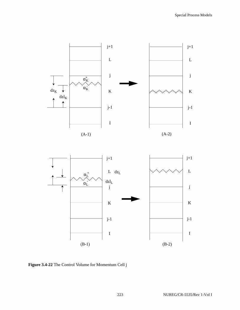
Special Process Models
Figure 3.4-22 The Control Volume for Momentum Cell j
j-1
K
j
L
(A-1)
dzK
dzlK
dzL
dzlL
αK+
αK-
αL+
αL-
j+1
j-1
K
j
L
(A-2)
j+1
I
I
j-1
K
j
L
j+1
I
j-1
K
j
L
j+1
I
(B-2)(B-1)
223 NUREG/CR-5535/Rev 1-Vol I
Special Process Models
The pressure gradient in the momentum cell must also be modified to accommodate the presence of
the mixture level. The pressure gradient in the momentum cell is computed as:
(3.4-117)
If there is a mixture level in the momentum cell, the pressure at one or the other end of the momentum cell
is modified. The pressure at the K end of the momentum cell is modified if the mixture level is in the K
volume, and the pressure at the L end of the momentum cell is modified if the mixture level is in the L
volume. The pressures are modified by extrapolating the pressure gradient in the junction below the
junction containing the mixture level. The junction below the one containing the mixture level is in bubbly
flow which has a large pressure gradient. Extrapolation of a large pressure gradient leads to a better
numerical performance since small errors in the computed pressure gradient leads to a smaller relative
error than extrapolation of small pressure gradients found in the junctions above the mixture level. The
pressures are modified as
(3.4-118)
(3.4-119)
where
(3.4-120)
for the situations shown in Figure 3.4-22 (A-1) and Figure 3.4-22 (B-1) respectively. If there is no
junction at the bottom or top of the volume containing the mixture level, the pressure gradient due to
gravity head is used to adjust the volume pressure.
The momentum flux terms are also modified in the momentum equations. These terms are set to zero
for the junctions above and below the volume containing the mixture level.
3.4.8.5 Modification of Heat Transfer Calculation.
When a heat structure is associated with a hydrodynamic volume where a mixture level exists, the
heat transfer will be partitioned according the level location (Figure 3.4-23). The heat fluxes from the wall
to the liquid and gas the phase (qwf and qwg) are calculated as:
zddP PL PK–
dzj------------------=
PK′ PK dzlK
dzK
2---------–
zd
dP
j 1–
+=
PL′ PL
dzL
2-------- dzlL–
zd
dP
j 1–
+=
zddP
j 1–
PK PI–dzj 1–
-----------------=
NUREG/CR-5535/Rev 1-Vol I 224
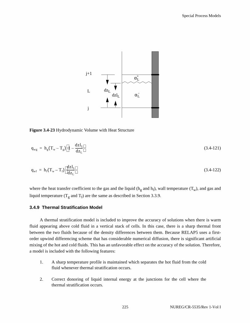
Special Process Models
(3.4-121)
(3.4-122)
where the heat transfer coefficient to the gas and the liquid (hg and hf), wall temperature (Tw), and gas and
liquid temperature (Tg and Tf) are the same as described in Section 3.3.9.
3.4.9 Thermal Stratification Model
A thermal stratification model is included to improve the accuracy of solutions when there is warm
fluid appearing above cold fluid in a vertical stack of cells. In this case, there is a sharp thermal front
between the two fluids because of the density differences between them. Because RELAP5 uses a first-
order upwind differencing scheme that has considerable numerical diffusion, there is significant artificial
mixing of the hot and cold fluids. This has an unfavorable effect on the accuracy of the solution. Therefore,
a model is included with the following features:
1. A sharp temperature profile is maintained which separates the hot fluid from the coldfluid whenever thermal stratification occurs.
2. Correct donoring of liquid internal energy at the junctions for the cell where thethermal stratification occurs.
Figure 3.4-23 Hydrodynamic Volume with Heat Structure
j
L
j+1
dzLdzlL
αL+
αL-
qwg hg Tw Tg–( ) 1dzlL
dzL----------–
=
qwf hf Tw Tf–( )dzlL
dzL----------
=
225 NUREG/CR-5535/Rev 1-Vol I

Special Process Models
3. Only the hot fluid in a cell which contains the thermal front is allowed to flash.
In addition, the model is compatible with the mixture level model and when used in conjunction with
the level model, it allows the code to predict the stratified behavior in a tank with considerable accuracy.
There are essentially two good choices to meet the requirements stated above. One possibility is to
use a Godunov-type scheme with artificial compression method to sharpen the temperature profile at the
edge of the cell. The second approach is to use Harten’s subcell resolution scheme,3.4-44 to track the front
in the interior of the cell. The problem with the first approach is that the front is tracked at the edge of the
cell, whereas the front spends most of its time in the interior of the cell. Among other things, criteria 2 and
3 of the above may never be satisfied. This is not a serious problem for CFD codes where cell size tends to
be fairly small. For engineering codes that use coarse nodalization, Harten’s approach is the best approach
if it is applicable to the problems in question.
It should be emphasized that although the proposed model can be viewed as an extension of Harten’s
method to the liquid internal energy for two-phase flow problems, the implementation of the model draws
heavily from that of the mixture level model. Still, to have a deeper understanding of the range of
applicability of the method, the reader is strongly encouraged to read Harten’s paper. In the thermal model,
the solution locally near the front is assumed to have a very simple profile. It is piecewise constant with the
larger positive value appearing on top of a smaller value. Because RELAP5 uses a simple first-order
scheme with positive coefficients, it is therefore possible to determine the position of the front accurately
using a simple calculation given in Section 3.4.9.3 below.
3.4.9.1 Overview of Software Design for the Thermal Stratification Model.
The thermal front is defined as the location where a sharp change in the temperature of the fluid
occurs. The thermal front tracking model implemented in RELAP5/MOD3 is analogous to the mixture
level tracking model currently in RELAP5/MOD3 (see Section 3.4.8), both in its methodology and in its
implementation. The model consists of four parts:
1. Detection of the thermal front appearance and disappearance.
2. Calculation of thermal front parameters that are necessary to describe a thermal frontsuch as the position and velocity of the front, and the temperatures above and belowthe front.
3. Modification of the liquid internal energy at the junctions to accurately convect theliquid internal energy above and below the front.
4. Modification of the heat transfer calculation and vapor generation rate according tothe position of the thermal front and temperature of the hot fluid in the cell thatcontains the thermal front.
NUREG/CR-5535/Rev 1-Vol I 226
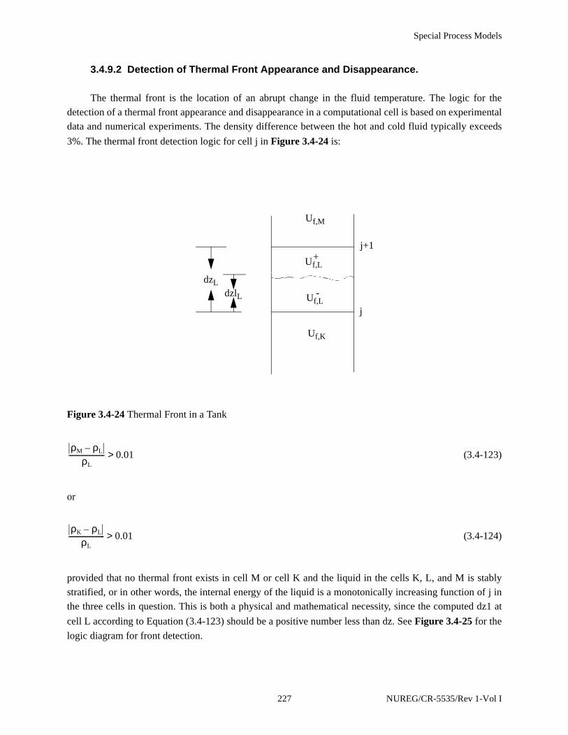
Special Process Models
3.4.9.2 Detection of Thermal Front Appearance and Disappearance.
The thermal front is the location of an abrupt change in the fluid temperature. The logic for the
detection of a thermal front appearance and disappearance in a computational cell is based on experimental
data and numerical experiments. The density difference between the hot and cold fluid typically exceeds
3%. The thermal front detection logic for cell j in Figure 3.4-24 is:
(3.4-123)
or
(3.4-124)
provided that no thermal front exists in cell M or cell K and the liquid in the cells K, L, and M is stably
stratified, or in other words, the internal energy of the liquid is a monotonically increasing function of j in
the three cells in question. This is both a physical and mathematical necessity, since the computed dz1 at
cell L according to Equation (3.4-123) should be a positive number less than dz. See Figure 3.4-25 for the
logic diagram for front detection.
Figure 3.4-24 Thermal Front in a Tank
Uf,M
Uf,L
Uf,K
dzLdzlL
j+1
j
+
Uf,L-
ρM ρL–ρL
--------------------- 0.01>
ρK ρL–ρL
--------------------- 0.01>
227 NUREG/CR-5535/Rev 1-Vol I
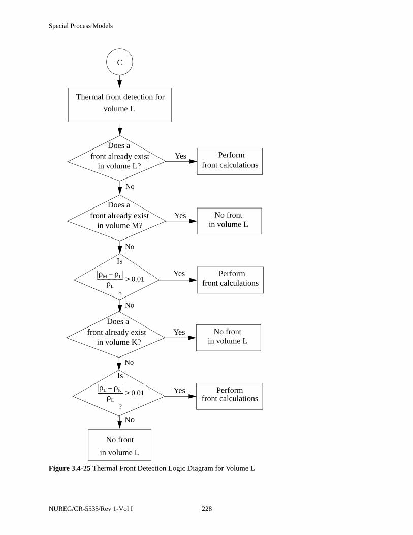
Special Process Models
Figure 3.4-25 Thermal Front Detection Logic Diagram for Volume L
ρM ρL–ρL
--------------------- 0.01>
C
Thermal front detection for
volume L
Does a front already exist Yes
in volume M?
Perform front calculations
Does a front already exist
in volume L?
No frontin volume L
Is
Performfront calculations
Performfront calculations
No front
in volume L
Yes
Yes
Yes
?
in volume K?
Does a front already exist No front
in volume L Yes
Is
ρL ρK–ρL
--------------------- 0.01>
?
No
No
No
No
Νο
NUREG/CR-5535/Rev 1-Vol I 228
Special Process Models
3.4.9.3 Calculation of Front Parameters.
The front parameters that describe the thermal front are:
1. The internal energy of the fluid above and below the front
2. The location of the front (dzlL)
3. the thermal front velocity (vfront)
3.4.9.3.1 Determination of the Internal Energy Above and Below the Front
The internal energy of the fluid below the front is set equal to the internal energy of the fluid in
volume K
(3.4-125)
while the internal energy of the fluid above the front is set equal to the internal energy of the fluid in
volume M
(3.4-126)
3.4.9.3.2 Location of the Thermal Front
Once the presence of a thermal front is determined in a particular volume, a flag is set and the front
parameters are calculated. The position of the front (dz1L) of a volume with length dzL is given by
(3.4-127)
where the and are given in Section 3.4.9.3.1. It is emphasized that this computation is performed
only when . This ensures that dz1L is a positive number less than dzL.
3.4.9.3.3 Velocity of the Thermal Front
The velocity of the thermal front is computed from:
UfL+ and UfL
-( )
UfL- = Uf K,
UfL+ = Uf M,
dz1L dzL
UfL+ UfL–
UfL+ UfL
-–----------------------
=
UfL+ UfL
-
UfL+ UfL UfL
-> >
229 NUREG/CR-5535/Rev 1-Vol I
Special Process Models
(3.4-128)
3.4.9.3.4 Modifications for Front Crossing
The criteria to determine if a thermal front will cross a cell boundary area
1. For a rising front, vfront > 0,
(3.4-129)
or
(3.4-130)
This is the case when the thermal front is near the top of volume L and the densities ρL and are
very close.
2. For a falling front, vfront < 0
(3.4-131)
or
(3.4-132)
This is the case when the thermal front is near the bottom of volume L and the densities ρL and
are very close. Figure 3.4-26 shows the logic diagram for the computation of thermal front parameters
with modifications for front crossing.
vfront
dz1Ln dz1L
n 1––∆t
-----------------------------------=
ρL ρL-–
ρL-------------------- 0.001<
dz1L
dzL----------- 0.98≥
ρL-
ρL+ ρL–ρL
-------------------- 0.001<
dz1L
dzL----------- 0.02≤
ρL+
NUREG/CR-5535/Rev 1-Vol I 230

Special Process Models
Figure 3.4-26 Computation of Thermal Front Parameters Logic Diagram for Volume L
C
Thermal front calculationfor volume L
Is thefluid stably
stratified in cells
K, L, M?
Set frontparameters to zero
Set frontparameters to zero
Set frontparameters to zero
No
Yes
Yes
Yes
No
No
Compute from parametersusing Equations (3.4-127)
and (3.4-128)
Is thefirst criterion
for front crossing
satisfied?
Is thesecond criterion
for front crossingsatisfied?
Thermal frontcalculated
for volume L
231 NUREG/CR-5535/Rev 1-Vol I

Special Process Models
3.4.9.4 Modification of RELAP5 Field Equations for Front Tracking.
The following modifications were made in solving the field equations in RELAP5:
1. The donor cell liquid internal energy based on the liquid internal energy above andbelow the thermal front will be used in the field equations.
2. The liquid temperature in the cell that contains the thermal front is modified in thecomputation of mass and energy transfer to indicate that only the hot fluid in the cellcan undergo phase change, (i.e., flash to vapor).
3. The interphase heat transfer coefficient in the cell that contains the thermal front ismodified to indicate that only the hot fluid in the cell can flash.
3.4.9.4.1 Donor Cell Internal Energy Formulation
The donor internal energies to be used at junctions j+1 and j in the field equations are given in Table
3.4-2.
3.4.9.4.2 Modifications of Mass and Energy Transfer Calculation
Because only hot fluid in the cell that contains the thermal front can flash, the interfacial heat transfer
coefficients need to be recalculated to reflect this. If the thermal front occurs at cell L, then Hif will be
recomputed as
(3.4-133)
The contribution to the vapor generation by the term Hif (Ts - TfL) is then modified to be
Table 3.4-2 Logic for Determining Donor Internal Energy
Junction vg vf
j+1 above front > 0 ug,L > 0 uf,M
j+1 above front < 0 ug,M < 0 uf,M
j below front > 0 ug,K > 0 uf,K
j below front < 0 ug,L < 0 uf,K
v 0 Rising Fluid↔>( )
U· g U· f
Hifnew Hif 1
dz1L
dzL-----------–
=
NUREG/CR-5535/Rev 1-Vol I 232
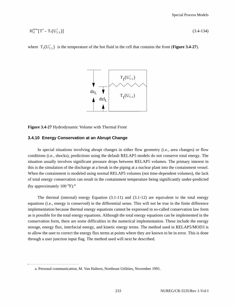
Special Process Models
(3.4-134)
where is the temperature of the hot fluid in the cell that contains the front (Figure 3.4-27).
3.4.10 Energy Conservation at an Abrupt Change
In special situations involving abrupt changes in either flow geometry (i.e., area changes) or flow
conditions (i.e., shocks), predictions using the default RELAP5 models do not conserve total energy. The
situation usually involves significant pressure drops between RELAP5 volumes. The primary interest in
this is the simulation of the discharge at a break in the piping at a nuclear plant into the containment vessel.
When the containment is modeled using normal RELAP5 volumes (not time-dependent volumes), the lack
of total energy conservation can result in the containment temperature being significantly under-predicted
(by approximately 100 oF).a
The thermal (internal) energy Equation (3.1-11) and (3.1-12) are equivalent to the total energy
equations (i.e., energy is conserved) in the differential sense. This will not be true in the finite difference
implementation because thermal energy equations cannot be expressed in so-called conservation law form
as is possible for the total energy equations. Although the total energy equations can be implemented in the
conservation form, there are some difficulties in the numerical implementation. These include the energy
storage, energy flux, interfacial energy, and kinetic energy terms. The method used in RELAP5/MOD3 is
to allow the user to correct the energy flux terms at points where they are known to be in error. This is done
through a user junction input flag. The method used will next be described.
Figure 3.4-27 Hydrodynamic Volume with Thermal Front
a. Personal communication, M. Van Haltern, Northeast Utilities, November 1991.
Hifnew Ts T– f Uf L,
+( )[ ]
Tf Uf L,+( )
dzL
dzlL
Tf Uf L,+( )
Tf Uf L,-( )
233 NUREG/CR-5535/Rev 1-Vol I

Special Process Models
The vapor thermal energy equation will be used to describe the method. The liquid thermal energy
equation is similar. The nonexpanded vapor thermal energy Equation (3.1-112) is of the finite difference
form
(3.4-135)
where RHS is the right-hand side terms. If the vapor velocity is positive through junctions j and j+1, the
pressure used in the energy flux term for junction j is rather than . Thus, Equation (3.4-135)
becomes
(3.4-136)
For positive vapor velocity in junction j, the donored density and the donored energy , will
also be from volume K. Thus, the energy flux term for junction j is really the enthalpy from volume K.
This modification results in using internal energy in the time derivative and enthalpy in the convective
terms. This is the approach used in the containment code CONTAIN.3.4-45 In the CONTAIN code, the total
energy equation is the starting equation, but the kinetic energy is then ignored in the time derivative and
convective terms because typical containment volumes are quite large. The resultant time derivative and
convective terms are the same as shown in Equation (3.4-136). Using CONTAIN and the RELAP5
modification to the energy flux give results that correctly match the containment temperature.
3.4.11 Jet Junction Model
Jet junctions are used where subcooled water is injected into the bottom of a vertically stratified pool.
The fluid from the jet causes a stirring action in the pool to increase the condensation rate on the surface of
the pool. The surface turbulence intensity is a function of the distance of the surface from the jet, the pool
diameter, the jet Reynolds number, and fluid properties such as the Prandtl and Jacob numbers. The details
of the model are discussed in the closure relations section of Volume IV.
3.4.12 References
3.4-1. V. H. Ransom and J. A. Trapp. “The RELAP5 Choked Flow Model and Application to a LargeScale Flow Test.” Proceedings of the ANS/ASME/NRC International Topical Meeting on NuclearReactor Thermal-Hydraulics, Saratoga Springs, New York, October 5-8, 1980. pp. 799-819.
VL αgρgUg( )Ln 1+ αgρgUg( )L
n–[ ] α[ ·g j 1+,n
ρ· g j 1+,n
U· g j 1+,n
PLn+( )vg j 1+,
n 1+ Aj 1++
α· g j,n ρ· g j,
nU· g j,
nPL
n+( )vg j,n 1+ Aj ]∆ t– RHS=
PKn PL
n
VL αgρgUg( )Ln 1+ αgρgUg( )L
n–[ ] α[ ·g j 1+,n
ρ· g j 1+,n
U· g j 1+,n
PLn+( )vg j 1+,
n 1+ Aj 1++
α· g j,n ρ· g j,
nU· g j,
nPK
n+( )vg j,n 1+ Aj ]∆ t– RHS=
ρ· g j, U· g j,
NUREG/CR-5535/Rev 1-Vol I 234

Special Process Models
3.4-2. J. A. Trapp and V. H. Ransom. “A Choked-Flow Calculation Criterion for Nonhomogeneous.Nonequilibrium Two-Phase Flows.” International Journal of Multiphase Flow. 8. 6. 1982. pp.669-681.
3.4-3. P. R. Garabedian. Partial Differential Equations. New York: John Wiley and Sons. 1964.
3.4-4. G. B. Whitham. Linear and Nonlinear Waves. New York: John Wiley and Sons. 1974.
3.4-5. A. H. Shapiro. The Dynamics and Thermodynamics of Compressible Fluid Flow, II. New York:Ronald. 1954.
3.4-6. V. H. Ransom and J. A. Trapp. RELAP5 Progress Summary, Analytical Choking Criterion forTwo-Phase Flow. CDAP-TR-013. Idaho National Engineering Laboratory. 1978.
3.4-7. D. A. Drew, L. Y. Cheng, and R. T. Lahey, Jr. “The Analysis of Virtual Mass Effects in Two-Phase Flow.” International Journal of Multiphase Flow. 5. 1979. pp. 233-242.
3.4-8. P. S. Anderson, P. Astrup, L. Eget, and O. Rathman. “Numerical Experience with the Two-FluidModel RISQUE.” Proceedings from Topical Meeting on Thermal Reactor Safety, Sun Valley, ID.July 31-August 4, 1977.
3.4-9. D. Gidaspow (Chairman). “Modeling of Two-Phase Flow.” Proceedings of Round TableDiscussion RT-1-2 at the Fifth International Heat Transfer Conference. Tokyo, Japan. September3-7, 1974. also in ASME Journal of Heat Transfer. 3. 1974.
3.4-10. J. D. Ramshaw and J. A. Trapp. “Characteristics, Stability, and Short-Wavelength Phenomena inTwo-Phase Flow Equation Systems.” Nuclear Science and Engineering. 66. 1978. pp. 93-102.
3.4-11. N. Zuber. “On the Dispersed Two-Phase Flow in the Laminar Flow Regime.” ChemicalEngineering Science. 19. 1964. pp. 897-917.
3.4-12. N. Abuaf, O. C. Jones, Jr., and B. J. C. Wu. Critical Flashing Flow in Nozzles with SubcooledInlet Conditions. BNL-NUREG-27512. Brookhaven National Laboratory. 1980.
3.4-13. M. D. Alamgir and J. H. Lienhard. “Correlation of Pressure Undershoot During Hot WaterDepressurization.” Transactions of ASME, Journal of Heat Transfer. 103. 1981. pp. 52-73.
3.4-14. O. C. Jones, Jr. “Flashing Inception in Flowing Liquids.” Transactions of ASME, Journal of HeatTransfer. 102. 1980. pp. 439-444.
3.4-15. J. W. Burnell. “Flow of Boiling Water through Nozzles, Orifices, and Pipes.” Engineering. 1947.pp. 572-576.
3.4-16. F. J. Moody. “Maximum Flow Rate of a Single-Component, Two-Phase Mixture.” Transactionsof ASME, Journal of Heat Transfer. 87. 1965. pp. 134-142.
235 NUREG/CR-5535/Rev 1-Vol I
Special Process Models
3.4-17. W. M. Bryce. Improvements to the RELAP5/MOD1/014 LOCA Code: The RELAP5/MOD1/WIN001 Code. AEEW-R-1649. Atomic Energy Establishment Winfrith. May 1983. pp. 64-65.
3.4-18. K. H. Ardron and W. M. Bryce. Assessment of Horizontal Stratification Entrainment Model inRELAP5/MOD3. AEEW-R 2345. Atomic Energy Establishment Winfrith. April 1988.
3.4-19. W. M. Bryce. Numerics and Implementation of the UK Horizontal Stratification EntrainmentOff-Take Model into RELAP5/MOD3. AEA-TRS-1050, AEEW-R 2501. Atomic EnergyEstablishment Winfrith. March 1991.
3.4-20. J. A. Trapp and V. H. Ransom. RELAP5 Hydrodynamic Model Progress Summary--Abrupt AreaChanges and Parallel Branching. PG-R-77-92. Idaho National Engineering Laboratory.November 1977.
3.4-21. J. K. Vennard. “One-Dimensional Flow.” in: V. L. Streeter (ed.). Handbook of Fluid Dynamics.1st Edition. New York: McGraw Hill. 1961.
3.4-22. J. Weisman, T. Ake, and R. Knott. “Two-Phase Pressure Drop Across Abrupt Area Changes inOscillatory Flow.” Nuclear Science and Engineering. 61. 1976. pp. 297-309.
3.4-23. J. G. Collier. “Advanced Study Institute on Two-Phase Flows and Heat Transfer.” ASIProceedings. Istanbul, Turkey. August 1976.
3.4-24. M. M. El-Wakil. Nuclear Heat Transport. Scranton: International Textbook Company. 1971.
3.4-25. B. Harsch, A. Hussain, and J. Weisman. Two-Phase Pressure Drop Across Restrictions andOther Abrupt Area Changes. NUREG-0062. April 1976.
3.4-26. P. A. Lottes. “Expansion Losses in Two-Phase Flows.” Nuclear Science and Energy. 9. 1961. pp.26-31.
3.4-27. G. B. Wallis. One-Dimensional Two-Phase Flow. New York: McGraw-Hill Book Company.1969. pp. 336-341.
3.4-28. A. Cicchitti et al. “Two-Phase Cooling Experiments-Pressure Drop, Heat Transfer, and BurnoutMeasurements.” Energi Nucl.. 7. 1960. pp. 407-425.
3.4-29. D. R. Liles et al. TRAC-PF1/MOD1: Correlations and Models. NUREG/CR-5069, LA-11208-MS. Los Alamos National Laboratory. December 1988.
3.4-30. J. H. Mahaffy and D. R. Liles. “Numerically Induced Pressure Excursions in Two-Phase FlowCalculations.” 2nd International Topical Meeting on Nuclear Reactor Thermal Hydraulics.Santa Barbara, CA. January 11-14. 1983.
3.4-31. V. H. Ransom et al. RELAP5/MOD0 Code Description, Volume 2, Code Development Updateand Sample Problems. CDAP-TR-057. Idaho National Engineering Laboratory. May 1979.
NUREG/CR-5535/Rev 1-Vol I 236
Special Process Models
3.4-32. R. Riemke. “Countercurrent Flow Limitation Model for RELAP5/MOD3.” Nuclear Technology.93. 1991. pp. 166-173.
3.4-33. S. G. Bankoff, R. S. Tankin, M. C. Yuen, and C. L. Hsieh. “Countercurrent Flow of Air/Waterand Steam/Water Through a Horizontal Perforated Plate.” International Journal of Heat andMass Transfer. 14. 1981. pp. 1381-1385.
3.4-34. M. W. Cappiello. A Description of the TRAC-PF1/MOD1 CCFL Model. LA-UR-87-294. LosAlamos National Laboratory. 1987.
3.4-35. C. L. Tien, K. S. Chung, and C. P. Liu. Flooding in Two-Phase Countercurrent Flows. EPRI NP-984. February 1979.
3.4-36. B. Aktas. Improvements to the Two-Phase Water Level Modeling of a Transient Reactor AnalysisCode. MS Dissertation: Pennsylvania State University. 1995.
3.4-37. J. A. Borkowski, et al. TRAC-BF1/MOD1 Models and Correlations. NUREG/CR-4391, EGG-2680. Idaho National Engineering Laboratory. 1992.
3.4-38. B. Aktas and J. Mahaffy. “A Two-Phase Level Tracking Method.” Department of NuclearEngineering. Pennsylvania State University, submitted for publication in Nuclear Engineeringand Design.
3.4-39. B. Aktas and J. Mahaffy. “Enhanced Numerical Modeling of Manometer Based Oscillations ByDiscontinuity Tracking.” Transactions of the American Nuclear Society. Vol. 73. pp 503-504.San Francisco CA. November, 1995.
3.4-40. Y. K. Cheung, V. Parameswaran, and J. C. Shaug. BWR Refill-Reflood Program Task, 4.7-ModelDevelopment, TRAC-BWR Component Models. NUREG/CR-2574, EPRI NP-2376, GEAP-22052. April 1983.
3.4-41. D. D. Taylor. 1-D Level Tracking Model. IS-NSMD-83-011. Idaho National EngineeringLaboratory. April 1983.
3.4-42. A. Rosen et al. Teploenergetikia. 1976. Vol. 11. pp. 59
3.4-43. S. Z. Rouhani. Modified Correlations for Void and Pressure Drop. AB Atomenergi: Sweden.Internal Report No. AE-RTV 841. March 1969.
3.4-44. A. Harten. “End Schemes with Subcell Resolution.” Journal of Computational Physics. 83.1989. pp. 148-184.
3.4-45. K. W. Washington et al. Reference Manual for the CONTAIN 1.1 Code for Containment SevereAccident Analysis. NUREG/CR-5715, SAND91-0835. Sandia National Laboratory. May 1991.
237 NUREG/CR-5535/Rev 1-Vol I

Special Process Models
NUREG/CR-5535/Rev 1-Vol I 238

Component Models
3.5 Component Models
RELAP5 consists of a variety of generic models that are used to build system models. These include
the pipe, annulus, branch, single-volume, single-junction, etc., and will be discussed in more detail in
Volume II of this manual. The general philosophy has been to avoid system component models such as
steam generator and core. However, certain subsystem components are unavoidable due to unique
processes or performance. RELAP5 contains models for subsystem components such as a branch,
separator, jet mixer, pump, turbine, valve, accumulator, ECC mixer, and annulus. A brief summary of each
of these models is included here.
3.5.1 Branch
The branch component is a model designed for convenient interconnection of hydrodynamic
components. The identical result can be obtained by using a single-volume component and several single-
junction components. Thus, the branch is a separate component only in the input processing scheme.
The crossflow junction has been added in which the junction velocities are assumed to be normal to
the one-dimensional flow path of the hydrodynamic volume. Thus, the branch component can include
multiple connections at the inlet, outlet, or in the crossflow direction.
Specialized modeling considerations are applied to any volume having multiple junctions connected
at either volume end. (The ends of a hydrodynamic volume are the inlet and outlet, as defined in Section
3.1.1.)
These special calculations include both the method for calculating the volume average velocities and
the method for partitioning the volume cross-sectional area between the multiple inlet or multiple outlet
junctions. The partitioned volume areas are used both in the abrupt area change model, to calculate
junction kinetic loss factors, and in the momentum equations, to simulate the stream-tube area.
In applications, the multiple junction and crossflow models are used in three distinct ways to model
branching flows. These are a one-dimensional branch, a tee branch, and a crossflow branch. A combination
of the three basic branches may also occur. Each of the three basic models will be discussed in turn.
3.5.1.1 One-Dimensional Branch.
This basic branch model is consistent with the one-dimensional approximation for a piping network
and assumes that multidimensional effects at branches are small compared to system interaction effects. In
the case of branched flows that occur in headers or plena, the model gives an accurate physical description
of the flow division or merging process; and the one-dimensional branch model is intended primarily for
use in modeling such branched flows. Examples of such situations in LWR systems are flow division at the
core inlet if parallel flow paths through the core are modeled, steam generator inlet and outlet plena when
several parallel tube groups are modeled (for the effect of tube height and length), or at a wye connection.
239 NUREG/CR-5535/Rev 1-Vol I
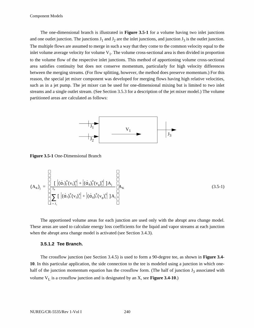
Component Models
The one-dimensional branch is illustrated in Figure 3.5-1 for a volume having two inlet junctions
and one outlet junction. The junctions J1 and J2 are the inlet junctions, and junction J3 is the outlet junction.
The multiple flows are assumed to merge in such a way that they come to the common velocity equal to the
inlet volume average velocity for volume V1. The volume cross-sectional area is then divided in proportion
to the volume flow of the respective inlet junctions. This method of apportioning volume cross-sectional
area satisfies continuity but does not conserve momentum, particularly for high velocity differences
between the merging streams. (For flow splitting, however, the method does preserve momentum.) For this
reason, the special jet mixer component was developed for merging flows having high relative velocities,
such as in a jet pump. The jet mixer can be used for one-dimensional mixing but is limited to two inlet
streams and a single outlet stream. (See Section 3.5.3 for a description of the jet mixer model.) The volume
partitioned areas are calculated as follows:
(3.5-1)
The apportioned volume areas for each junction are used only with the abrupt area change model.
These areas are used to calculate energy loss coefficients for the liquid and vapor streams at each junction
when the abrupt area change model is activated (see Section 3.4.3).
3.5.1.2 Tee Branch.
The crossflow junction (see Section 3.4.5) is used to form a 90-degree tee, as shown in Figure 3.4-
10. In this particular application, the side connection to the tee is modeled using a junction in which one-
half of the junction momentum equation has the crossflow form. (The half of junction J3 associated with
volume VL is a crossflow junction and is designated by an X, see Figure 3.4-10.)
Figure 3.5-1 One-Dimensional Branch
V1J3
J2
J1
AK( )j
α· f( )jn
vf( )jn α· g( )j
nvg( )j
n +[ ] Aj
α· f( )in
vf( )in α· g( )i
nvg( )i
n +[ ] Ai
i J1=
JN
∑-------------------------------------------------------------------------------------
AK=
NUREG/CR-5535/Rev 1-Vol I 240
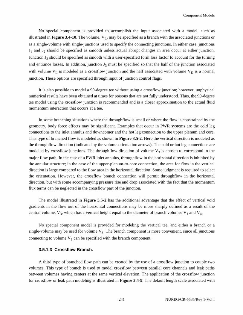
Component Models
No special component is provided to accomplish the input associated with a model, such as
illustrated in Figure 3.4-10. The volume, VL, may be specified as a branch with the associated junctions or
as a single-volume with single-junctions used to specify the connecting junctions. In either case, junctions
J1 and J2 should be specified as smooth unless actual abrupt changes in area occur at either junction.
Junction J3 should be specified as smooth with a user-specified form loss factor to account for the turning
and entrance losses. In addition, junction J3 must be specified so that the half of the junction associated
with volume VL is modeled as a crossflow junction and the half associated with volume VK is a normal
junction. These options are specified through input of junction control flags.
It is also possible to model a 90-degree tee without using a crossflow junction; however, unphysical
numerical results have been obtained at times for reasons that are not fully understood. Thus, the 90-degree
tee model using the crossflow junction is recommended and is a closer approximation to the actual fluid
momentum interaction that occurs at a tee.
In some branching situations where the throughflow is small or where the flow is constrained by the
geometry, body force effects may be significant. Examples that occur in PWR systems are the cold leg
connections to the inlet annulus and downcomer and the hot leg connection to the upper plenum and core.
This type of branched flow is modeled as shown in Figure 3.5-2. Here the vertical direction is modeled as
the throughflow direction (indicated by the volume orientation arrows). The cold or hot leg connections are
modeled by crossflow junctions. The throughflow direction of volume V3 is chosen to correspond to the
major flow path. In the case of a PWR inlet annulus, throughflow in the horizontal direction is inhibited by
the annular structure; in the case of the upper-plenum-to-core connection, the area for flow in the vertical
direction is large compared to the flow area in the horizontal direction. Some judgment is required to select
the orientation. However, the crossflow branch connection will permit throughflow in the horizontal
direction, but with some accompanying pressure rise and drop associated with the fact that the momentum
flux terms can be neglected in the crossflow part of the junction.
The model illustrated in Figure 3.5-2 has the additional advantage that the effect of vertical void
gradients in the flow out of the horizontal connections may be more sharply defined as a result of the
central volume, V3, which has a vertical height equal to the diameter of branch volumes V1 and V4.
No special component model is provided for modeling the vertical tee, and either a branch or a
single-volume may be used for volume V3. The branch component is more convenient, since all junctions
connecting to volume V3 can be specified with the branch component.
3.5.1.3 Crossflow Branch.
A third type of branched flow path can be created by the use of a crossflow junction to couple two
volumes. This type of branch is used to model crossflow between parallel core channels and leak paths
between volumes having centers at the same vertical elevation. The application of the crossflow junction
for crossflow or leak path modeling is illustrated in Figure 3.4-9. The default length scale associated with
241 NUREG/CR-5535/Rev 1-Vol I

Component Models
the crossflow junction is one-half the diameter of the K volume plus one half the diameter of the L volume.
This length is only used for modeling the fluid inertia terms in the momentum equation. The user has the
option to input the length for a crossflow junction.
The pure crossflow branch is most easily modeled using a single-junction component for the
crossflow junction. However, either volume V1 or V2 in Figure 3.4-9 can be modeled using the branch
component and specifying the coupling junctions with that component.
3.5.2 Separator
The separator component model has two options, the simple separator model which was
implemented in previous versions of RELAP5 and a mechanistic separator model intended to model the
centrifugal separators and chevron dryers in BWR reactors. The separator model determines the convected
void fractions in the liquid fall back junction and the vapor outlet junction.
3.5.2.1 Simple Separator.
The model is a nonmechanistic or black-box model consisting of a special volume with junction
flows, as pictured in Figure 3.5-3. A steam-water inflowing mixture is separated by defining the quality of
the outflow streams using empirical functions. No attempt is made to model the actual separation process
from first principles.
The separator vapor outlet performance is defined by means of a special function for the vapor void
fraction at J1. The donored junction vapor void fraction used to flux mass through the steam outlet is
Figure 3.5-2 Gravity Effects on a Tee
V2
V4V3
J2
J1
V1
V5
J3J4
XX
NUREG/CR-5535/Rev 1-Vol I 242
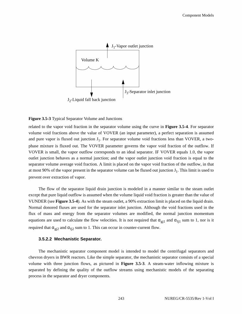
Component Models
related to the vapor void fraction in the separator volume using the curve in Figure 3.5-4. For separator
volume void fractions above the value of VOVER (an input parameter), a perfect separation is assumed
and pure vapor is fluxed out junction J1. For separator volume void fractions less than VOVER, a two-
phase mixture is fluxed out. The VOVER parameter governs the vapor void fraction of the outflow. If
VOVER is small, the vapor outflow corresponds to an ideal separator. IF VOVER equals 1.0, the vapor
outlet junction behaves as a normal junction; and the vapor outlet junction void fraction is equal to the
separator volume average void fraction. A limit is placed on the vapor void fraction of the outflow, in that
at most 90% of the vapor present in the separator volume can be fluxed out junction J1. This limit is used to
prevent over extraction of vapor.
The flow of the separator liquid drain junction is modeled in a manner similar to the steam outlet
except that pure liquid outflow is assumed when the volume liquid void fraction is greater than the value of
VUNDER (see Figure 3.5-4). As with the steam outlet, a 90% extraction limit is placed on the liquid drain.
Normal donored fluxes are used for the separator inlet junction. Although the void fractions used in the
flux of mass and energy from the separator volumes are modified, the normal junction momentum
equations are used to calculate the flow velocities. It is not required that αgj1 and αfj1 sum to 1, nor is it
required that αgj2 and αfj2 sum to 1. This can occur in counter-current flow.
3.5.2.2 Mechanistic Separator.
The mechanistic separator component model is intended to model the centrifugal separators and
chevron dryers in BWR reactors. Like the simple separator, the mechanistic separator consists of a special
volume with three junction flows, as pictured in Figure 3.5-3. A steam-water inflowing mixture is
separated by defining the quality of the outflow streams using mechanistic models of the separating
process in the separator and dryer components.
Figure 3.5-3 Typical Separator Volume and Junctions
Volume K
J1-Vapor outlet junction
J3-Separator inlet junction
J2-Liquid fall back junction
243 NUREG/CR-5535/Rev 1-Vol I

Component Models
3.5.2.2.1 Centrifugal Separator Model
The model for the centrifugal separator was taken from the TRAC-BWR computer code and was
developed by the General Electric Company as part of the joint USNRC- EPRI- General Electric Company
sponsored BWR Refill-Reflood Program. Separators are made up of either two- or three-stages connected
in series. The separator model determines the separating efficiency of a single-stage, feeding the output of
one stage to the input of the next stage. The primary measures of separator performance are carryover of
entrained liquid in the steam leaving the separator, carryunder of steam in the liquid leaving the discharge
passage of the separator, and the separator pressure drop. A mechanistic model has been developed to
calculate the carryover, carryunder, and separator pressure drop. The separator component volume as
shown in Figure 3.5-3 represents the physical volume in the separator barrel and discharge passages. The
inlet junction J3 represents the flow from the separator standpipe through the swirl vanes to the separator
barrel. The vapor outlet junction J1 represents the flow out of the top of the separating barrel from the last
separating stage and the liquid outlet junction J2 represents the combined discharge passages of all of the
stages. The following description of the mechanistic separator model is adapted from Reference 3.5-1.
A separator component consists of three regions, a standpipe, the separator barrel, and the discharge
passage. Figure 3.5-5 shows a schematic of the first stage of a separator component. A two-phase mixture
enters the separator barrel from the standpipe, passing through a set of stationary swirl vanes attached to
the separator hub which acts as a bladed nozzle. These vanes produce a high rotational velocity component
Figure 3.5-4 Donor Junction Voids for Outflow
Vapor outlet
1.0VOVER
1.0
0.0
junction
αgK
Liquid fall back
1.0VUNDER
1.0
0.0
junction
αfK
αgJ1
αfJ2
NUREG/CR-5535/Rev 1-Vol I 244

Component Models
in the fluid flowing through the separator barrel. The resultant centrifugal force separates the steam-water
mixture into a water vortex on the inner wall of the separating barrel and a steam vortex core. Separation is
accomplished by directing the water layer on the wall into the discharge passage through pick-off rings at
the exit of the separator barrel.
3.5.2.2.2 Assumptions and Model Equations
In this model, the following assumptions are made for the axial location near the pick-off ring:
1. There is one uniform axial velocity in each of the flow regions, i.e.
Figure 3.5-5 Schematic of First Stage of Mechanistic Separator
HD
Hsk
H12
Standpipe
HUBVan
rw
rw
Vaporcore
VD
Liquid layer
rr
rfVaf
Vag
Pickoff ring
Discharge passage
Vi,Pi,ρmi
245 NUREG/CR-5535/Rev 1-Vol I
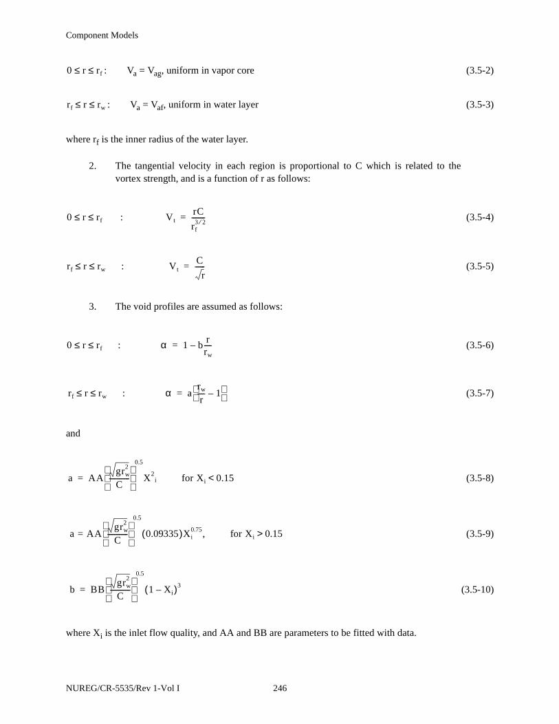
Component Models
: Va = Vag, uniform in vapor core (3.5-2)
: Va = Vaf, uniform in water layer (3.5-3)
where rf is the inner radius of the water layer.
2. The tangential velocity in each region is proportional to C which is related to thevortex strength, and is a function of r as follows:
(3.5-4)
(3.5-5)
3. The void profiles are assumed as follows:
(3.5-6)
(3.5-7)
and
(3.5-8)
(3.5-9)
(3.5-10)
where Xi is the inlet flow quality, and AA and BB are parameters to be fitted with data.
0 r rf≤ ≤
rf r rw≤ ≤
0 r rf : ≤ ≤ VtrC
rf3 2⁄--------=
rf r rw : ≤ ≤ VtC
r------=
0 r rf : ≤ ≤ α 1 brrw----–=
rf r rw : ≤ ≤ α arw
r---- 1–
=
a AAgrw
2
C------------
0.5
X2i= for Xi 0.15<
a AAgrw
2
C------------
0.5
0.09335( )Xi0.75= , for Xi 0.15>
b BBgrw
2
C------------
0.5
1 Xi–( )3=
NUREG/CR-5535/Rev 1-Vol I 246

Component Models
4. The pressure in the vapor core (Po) is assumed to be uniform radially and axially, and
the pressure at the separator wall (Pw) is related to Po by centrifugal force across the
water layer.
For the first stage of the separator, a total of six unknowns are introduced in this model. These are
Vag, Vaf, C, rf, Po, and Pw. The required equations are formulated from conservation of water mass, vapor
mass, axial momentum, and angular momentum entering and leaving the separating barrel, from
centrifugal pressure drop across the water layer and from pressure drop in the discharge passage. The
above unknowns can now be solved from given conditions of pressure, Pi, total flow rate, Wi, and flow
quality at the swirl vane inlet, Xi.
The mass and momentum conservation equations for flows entering and leaving the separating barrel
are:
Water mass
(3.5-11)
Vapor Mass
(3.5-12)
Angular Momentum
(3.5-13)
Axial Momentum
1 Xi–( )Wi 2π 1 α–( )ρfVar rd∫ 2πVagρf13---
rfbrw------
rf2= =
2πρfVaf1 a+
2------------
rw2 rf
2–( ) a rw rf–( )–[ ]
+
XiWi 2π αρgVgr rd
0
rw
∫ 2πρgVag12---
13---b
rf
rw----–
rf2= =
2πρgVafa12--- rw rf–( )2m+
Vtnr 2πrρmiVan( ) rd
rh
rw
∫ Vtr 2πrρVa( ) r Ftrw+d
0
rw
∫=
247 NUREG/CR-5535/Rev 1-Vol I
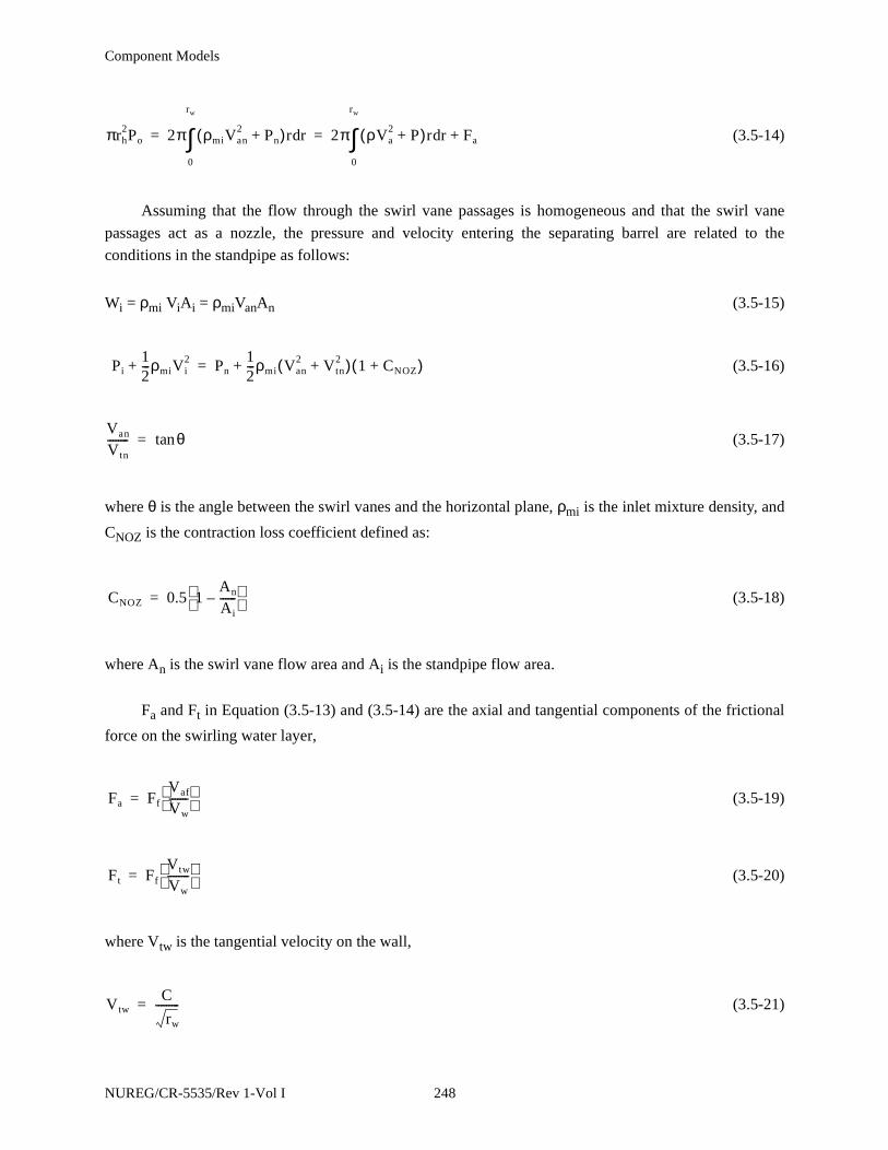
Component Models
(3.5-14)
Assuming that the flow through the swirl vane passages is homogeneous and that the swirl vane
passages act as a nozzle, the pressure and velocity entering the separating barrel are related to the
conditions in the standpipe as follows:
Wi = ρmi ViAi = ρmiVanAn (3.5-15)
(3.5-16)
(3.5-17)
where θ is the angle between the swirl vanes and the horizontal plane, ρmi is the inlet mixture density, and
CNOZ is the contraction loss coefficient defined as:
(3.5-18)
where An is the swirl vane flow area and Ai is the standpipe flow area.
Fa and Ft in Equation (3.5-13) and (3.5-14) are the axial and tangential components of the frictional
force on the swirling water layer,
(3.5-19)
(3.5-20)
where Vtw is the tangential velocity on the wall,
(3.5-21)
πrh2Po 2π ρmiVan
2 Pn+( )r rd
0
rw
∫ 2π ρVa2 P+( )r r Fa+d
0
rw
∫= =
Pi12---ρmiVi
2+ Pn12---ρmi Van
2 Vtn2+( ) 1 CNOZ+( )+=
Van
Vtn-------- θtan=
CNOZ 0.5 1An
Ai------–
=
Fa Ff
Vaf
Vw-------
=
Ft Ff
Vtw
Vw--------
=
VtwC
rw
---------=
NUREG/CR-5535/Rev 1-Vol I 248
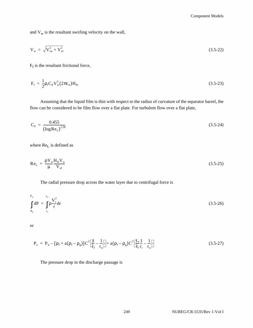
Component Models
and Vw is the resultant swirling velocity on the wall,
(3.5-22)
Ff is the resultant frictional force,
(3.5-23)
Assuming that the liquid film is thin with respect to the radius of curvature of the separator barrel, the
flow can be considered to be film flow over a flat plate. For turbulent flow over a flat plate,
(3.5-24)
where ReL is defined as
(3.5-25)
The radial pressure drop across the water layer due to centrifugal force is
(3.5-26)
or
(3.5-27)
The pressure drop in the discharge passage is
Vw Vtw2 Vaf
2+=
Ff12---ρfCFVw
2 2πrw( )HD=
CF0.455
ReLlog( )2.58-----------------------------=
ReL
ρVw
µ----------
HDVw
Vaf---------------=
Pd
P0
Pw
∫ ρVt
2
r------ rd
rf
rw
∫=
Po Pw ρf a ρf ρg–( )+[ ] C2 1rf---
1rw----–
– a ρf ρg–( )C2 rw
rf----
1rr---
1rw----–
+=
249 NUREG/CR-5535/Rev 1-Vol I
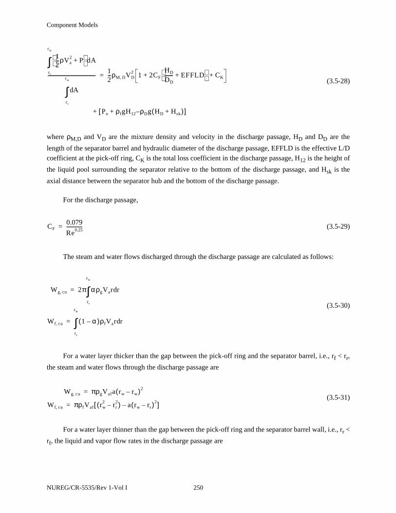
Component Models
(3.5-28)
where ρM,D and VD are the mixture density and velocity in the discharge passage, HD and DD are the
length of the separator barrel and hydraulic diameter of the discharge passage, EFFLD is the effective L/D
coefficient at the pick-off ring, CK is the total loss coefficient in the discharge passage, H12 is the height of
the liquid pool surrounding the separator relative to the bottom of the discharge passage, and Hsk is the
axial distance between the separator hub and the bottom of the discharge passage.
For the discharge passage,
(3.5-29)
The steam and water flows discharged through the discharge passage are calculated as follows:
(3.5-30)
For a water layer thicker than the gap between the pick-off ring and the separator barrel, i.e., rf < rr,
the steam and water flows through the discharge passage are
(3.5-31)
For a water layer thinner than the gap between the pick-off ring and the separator barrel wall, i.e., rr <
rf, the liquid and vapor flow rates in the discharge passage are
12---ρVa
2 P+
rr
rw
∫ dA
Ad
rr
rw
∫----------------------------------------
12---ρM D, VD
2 1 2CF
HD
DD------- EFFLD+
CK+ +=
Po ρfgH12 ρD– g HD Hsk+( )+[ ]+
CF0.079
Re0.25-------------=
Wg cu, 2π αρgVar rd
rr
rw
∫=
Wf cu, 1 α–( )ρfVar rd
rr
rw
∫=
Wg cu, πρgVafa rw rw–( )2=
Wf cu, πρfVaf rw2 rr
2–( ) a rw rr–( )2–[ ]=
NUREG/CR-5535/Rev 1-Vol I 250

Component Models
(3.5-32)
The steam and water flows leaving the present stage and entering the next stage are
(3.5-33)
The total discharge flow is
WD = Wg,cu + Wf,cu (3.5-34)
Assuming homogeneous flow in the discharge passage, the mean void fraction is
(3.5-35)
the mixture density in the discharge passage is
ρM,D = αcuρg + (1 - αcu)ρf (3.5-36)
and the velocity in the discharge passage is
(3.5-37)
In summary, for given swirl vane inlet conditions, Pi, Xi, and Wi, the unknowns Vag, Vaf, C, rf, Po,
and Pw are calculated by solving Equation (3.5-11) to (3.5-28) simultaneously.
Similar equations can be written for the second- and third-stages. Since it is assumed that Po is
uniform axially, i.e., the vapor core pressure drop in the axial direction is small, the axial momentum
equation can be neglected in the solution for the upper stages. For these stages, the unknowns are reduced
to Vag, Vaf, C, rf, and Pw, and the equations are the conservation of water mass, vapor mass, angular
momentum, the pressure drop across the water layer, and the pressure drop in the discharge passage.
Wg cu, XiWi 2πρgVag12---
13---b
rr
rw----–
–= rr2
Wf cu, 1 Xi–( )Wi 2πρfVagrr2 1
2---
brr
rw----–=
Wg co, steam flow( )in Wg cu,–=
Wf co, water flow( )in Wf cu,–=
α cu
Wg cu,
Wg cu, Wf cu,ρg
ρf-----+
---------------------------------------=
VD
WD
ρM D, AD-------------------=
251 NUREG/CR-5535/Rev 1-Vol I
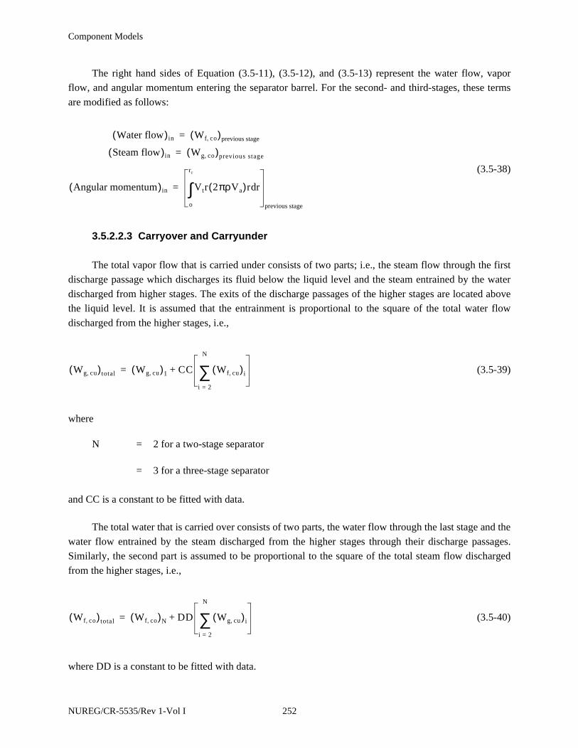
Component Models
The right hand sides of Equation (3.5-11), (3.5-12), and (3.5-13) represent the water flow, vapor
flow, and angular momentum entering the separator barrel. For the second- and third-stages, these terms
are modified as follows:
(3.5-38)
3.5.2.2.3 Carryover and Carryunder
The total vapor flow that is carried under consists of two parts; i.e., the steam flow through the first
discharge passage which discharges its fluid below the liquid level and the steam entrained by the water
discharged from higher stages. The exits of the discharge passages of the higher stages are located above
the liquid level. It is assumed that the entrainment is proportional to the square of the total water flow
discharged from the higher stages, i.e.,
(3.5-39)
where
N = 2 for a two-stage separator
= 3 for a three-stage separator
and CC is a constant to be fitted with data.
The total water that is carried over consists of two parts, the water flow through the last stage and the
water flow entrained by the steam discharged from the higher stages through their discharge passages.
Similarly, the second part is assumed to be proportional to the square of the total steam flow discharged
from the higher stages, i.e.,
(3.5-40)
where DD is a constant to be fitted with data.
Water flow( )in Wf co,( )previous stage=
Steam flow( )in Wg co,( )previous stage=
Angular momentum( )in Vtr 2πρVa( )r rd
o
rr
∫previous stage
=
Wg cu,( )total Wg cu,( )1 CC Wf cu,( )i
i 2=
N
∑+=
Wf co,( )total Wf co,( )N DD Wg cu,( )i
i 2=
N
∑+=
NUREG/CR-5535/Rev 1-Vol I 252
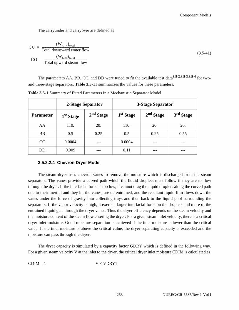
Component Models
The carryunder and carryover are defined as
(3.5-41)
The parameters AA, BB, CC, and DD were tuned to fit the available test data3.5-2,3.5-3,3.5-4 for two-
and three-stage separators. Table 3.5-11 summarizes the values for these parameters.
3.5.2.2.4 Chevron Dryer Model
The steam dryer uses chevron vanes to remove the moisture which is discharged from the steam
separators. The vanes provide a curved path which the liquid droplets must follow if they are to flow
through the dryer. If the interfacial force is too low, it cannot drag the liquid droplets along the curved path
due to their inertial and they hit the vanes, are de-entrained, and the resultant liquid film flows down the
vanes under the force of gravity into collecting trays and then back to the liquid pool surrounding the
separators. If the vapor velocity is high, it exerts a larger interfacial force on the droplets and more of the
entrained liquid gets through the dryer vanes. Thus the dryer efficiency depends on the steam velocity and
the moisture content of the steam flow entering the dryer. For a given steam inlet velocity, there is a critical
dryer inlet moisture. Good moisture separation is achieved if the inlet moisture is lower than the critical
value. If the inlet moisture is above the critical value, the dryer separating capacity is exceeded and the
moisture can pass through the dryer.
The dryer capacity is simulated by a capacity factor GDRY which is defined in the following way.
For a given steam velocity V at the inlet to the dryer, the critical dryer inlet moisture CDIM is calculated as
CDIM = 1 V < VDRY1
Table 3.5-1 Summary of Fitted Parameters in a Mechanistic Separator Model
2-Stage Separator 3-Stage Separator
Parameter 1st Stage 2nd Stage 1st Stage 2nd Stage 3rd Stage
AA 110. 20. 110. 20. 20.
BB 0.5 0.25 0.5 0.25 0.55
CC 0.0004 --- 0.0004 --- ---
DD 0.009 --- 0.11 --- ---
CUWg cu,( )total
Total downward water flow------------------------------------------------------------------=
COWf co,( )total
Total upward steam flow------------------------------------------------------------=
253 NUREG/CR-5535/Rev 1-Vol I

Component Models
(3.5-42)
= 0 VDRY2 < V
where CDIM is the critical inlet moisture, VDRY1 is the vapor velocity below which any amount of
moisture is assumed to be separated from the vapor stream, and VDRY2 is the vapor velocity above which
no amount of moisture, however small, can be separated from the vapor stream.
The dryer inlet moisture (DIM) is computed assuming homogeneous flow as
(3.5-43)
where αg, ρf, and ρg are the vapor void fraction, liquid density, and the vapor density in the dryer.
The capacity factor GDRY is defined as
GDRY = 1 DIM < CDIM
(3.5-44)
= 0 (CDIM + DELDIM) < DIM
where DELDIM is the range of inlet moisture over which the dryer capacity goes from one to zero for a
fixed vapor inlet velocity. These relations are shown schematically in Figure 3.5-6.
The capacity factor GDRY is used to modify the void fraction in the dryer outlet junction such that if
the dryer capacity is one, the donored void fraction is one; if the dryer capacity is zero, the regular donor
void fraction is used, and if the dryer capacity is between zero and one, the void fraction is interpolated
between the values for the capacities of zero and one.
3.5.3 Jet Mixer
There are several components in a typical reactor plant where the momentum effects due to the
mixing of two parallel streams of fluid at different velocities may be important. An example of this is the
jet pump in a BWR. In this component, the pumping action is caused by the momentum transfer between
the two fluid streams. Momentum effects may also be important for mixing at ECC injection points or for
1V VDRY1–
VDRY2 VDRY1–------------------------------------------------ VDRY1 V VDRY2< <–=
DIM 1αg
αg 1 α g–( )ρf
ρg-----+
--------------------------------------–=
1CDIM DIM–
DELDIM----------------------------------- CDIM < DIM < (CDIM + DELDIM)+=
NUREG/CR-5535/Rev 1-Vol I 254

Component Models
the aspirators present in some steam generators. The JETMIXER component was developed for these
cases.
3.5.3.1 Basic Jet Mixing Model.
The basic approach for modeling the jet mixing process is to superimpose a quasi-steady model for
the mixing process on the normal volume-junction flow path representation used in RELAP5. To derive
the momentum equations needed to model a jet mixing situation, consider the schematic shown in Figure
3.5-7, which illustrates a mixing volume connected to a drive and a suction volume.a The suction junction
(with velocity vS and area AS) connects the last upstream suction region volume, KS, to the mixing
volume, L. The drive junction (with velocity vD and area AD) connects the last upstream drive line volume,
KD, to the mixing volume, L. Figure 3.5-7 shows the drive junction as a smooth junction and the suction
junction as abrupt. The user can model either junction either way if the appropriate loss factors are
included (see input guidelines in Volume II of this manual). Void fractions and densities subscripted by a
D or S are donored values; a subscript a indicates an average value.
Figure 3.5-6 Dryer Capacity
a. The drive and suction junctions should be the high-speed and low-speed junctions respectively when the
JETMIXER component is used for other than jet pump applications.
100
50
Dry
er in
let m
oist
ure
(wei
ght%
)
above dotted line 0% separation
below solid line100% separation
Dryer inlet steam velocity
DELDIM
CDIM
VDRY1 VDRY2
V
between lineslinear interpolation
255 NUREG/CR-5535/Rev 1-Vol I
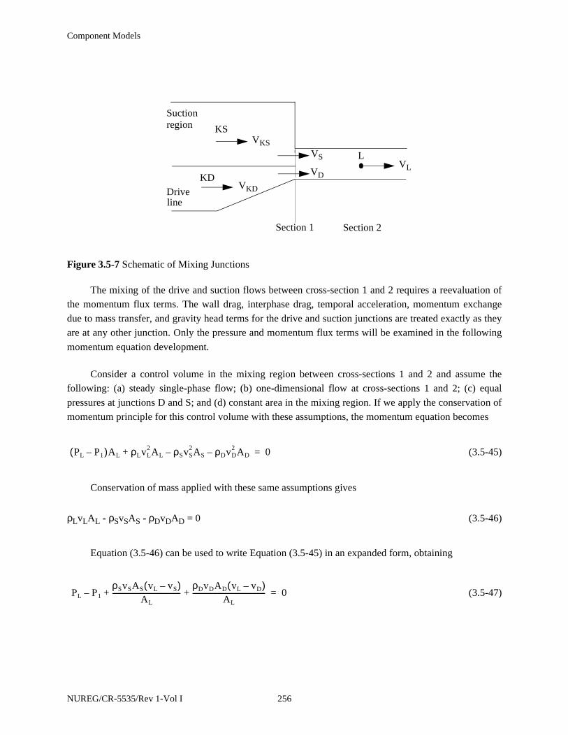
Component Models
The mixing of the drive and suction flows between cross-section 1 and 2 requires a reevaluation of
the momentum flux terms. The wall drag, interphase drag, temporal acceleration, momentum exchange
due to mass transfer, and gravity head terms for the drive and suction junctions are treated exactly as they
are at any other junction. Only the pressure and momentum flux terms will be examined in the following
momentum equation development.
Consider a control volume in the mixing region between cross-sections 1 and 2 and assume the
following: (a) steady single-phase flow; (b) one-dimensional flow at cross-sections 1 and 2; (c) equal
pressures at junctions D and S; and (d) constant area in the mixing region. If we apply the conservation of
momentum principle for this control volume with these assumptions, the momentum equation becomes
(3.5-45)
Conservation of mass applied with these same assumptions gives
ρLvLAL - ρSvSAS - ρDvDAD = 0 (3.5-46)
Equation (3.5-46) can be used to write Equation (3.5-45) in an expanded form, obtaining
(3.5-47)
Figure 3.5-7 Schematic of Mixing Junctions
Section 1 Section 2
Suctionregion KS
VKS
KDVD
VSVL
VKDDriveline
L
PL P1–( )AL ρLvL2 AL ρSvS
2AS– ρDvD2 AD–+ 0=
PL P1–ρSvSAS vL vS–( )
AL----------------------------------------
ρDvDAD vL vD–( )AL
-------------------------------------------+ + 0=
NUREG/CR-5535/Rev 1-Vol I 256
Component Models
Equation (3.5-47) gives the momentum equation (pressure and flux terms) for the upstream half of
the mixing volume. To develop the momentum equation for the suction junction, a normal RELAP5 half-
cell momentum equation is written from KS to cross-section 1, i.e.,
(3.5-48)
Adding this to the half cell momentum Equation (3.5-47) for cross-sections 1 to L (Section 2) gives
(3.5-49)
This equation shows how the pressure and momentum flux terms should be calculated for the suction
junction equation.
If the suction junction were a normal junction, its momentum equation (pressure and flux terms)
would be
(3.5-50)
The velocity terms in Equation (3.5-50) must be replaced by the velocity terms in Equation (3.5-49)
to correctly model the momentum equation at the suction junction. Similar equations for the drive junction
can be obtained.
3.5.3.2 Jet Mixing in Two-Phase Flows.
If a derivation similar to the previous section is carried out for the pressure and momentum flux
terms in the two-phase case, the following equations are obtained for the liquid phase in the mixing region:
Conservation of momentum (from cross-section 1 to L),
(3.5-51)
Conservation of mass (from cross-section 1 to L),
αfLρLvfLAL - αfSρfSvfSAfS - αfDρfDvfDAD = 0 (3.5-52)
P1 PKS–12---ρKS vS
2 vKS2–( )+ 0=
PL PKS–12---ρKS vS
2 vKS2–( )
ρSvSAS vL vS–( )AL
----------------------------------------+ρDvDAD vL vD–( )
AL-------------------------------------------++ 0=
PL PKS–12---ρS vL
2 vKS2–( )+ 0=
α fLAL PL P1–( ) α fLρfLvfL2 AL α fSρfSvfS
2 AS– α fDρfDvfD2 AD–+ 0=
257 NUREG/CR-5535/Rev 1-Vol I
Component Models
Using Equation (3.5-52) in Equation (3.5-51) and rewriting Equation (3.5-45) in expanded form
yields
(3.5−53)
Equation (3.5-53) can now be combined with the appropriate half-cell momentum equation for the
upstream volume to obtain the final momentum equation for the liquid flow at the suction junction. A
parallel development gives the gas-phase momentum equation at the suction junction.
The momentum equations used consist of the sum of the phasic momentum equations and the
difference of the phasic momentum equations. To derive the sum momentum equation (pressure and flux
terms only) for the suction junction, Equation (3.5-53) for the liquid phase is added to a similar equation
for the gas phase to obtain
(3.5-54)
The normal half-cell sum momentum equation (pressure and flux terms only) for the upstream
suction volume can then be added to Equation (3.5-54) to give
(3.5-55)
as the final form for the pressure and momentum flux terms in the new sum momentum equation for the
suction junction. The pressure term in this equation has exactly the same form as the pressure term in the
normal sum momentum equation. A parallel equation holds for the drive junction. Hence, at the drive and
suction mixing junctions, the normal momentum flux terms in the sum momentum equation must be
replaced by those in Equation (3.5-55).
The difference momentum equation for the suction junction is derived by dividing the liquid
momentum mixing Equation (3.5-53) by αfL and adding it to the half-cell liquid momentum equation for
the upstream suction volume (also divided by the appropriate void fraction, αfKS) to obtain
α fL PL P1–( )α fSρfSvfSAS vfL vfs–( )
AL------------------------------------------------------
α fDρfDvfDAD vfL vfD–( )AL
----------------------------------------------------------+ +
PL P1–α fSρfSvfSAS vfL vfS–( )
AL------------------------------------------------------
α fDρfDvfDAD vfL vrD–( )AL
----------------------------------------------------------+ +
αgSρgSvgSAS vgL vgS–( )AL
----------------------------------------------------------α gDρgDvgDAD vgL vgD–( )
AL-------------------------------------------------------------+ + 0=
PL PKS–α fSρfSvfSAS vfL vfS–( )
AL------------------------------------------------------
α fDρfDvfDAD vfL vfD–( )AL
----------------------------------------------------------+ +
αgSρgSvgSAS vgL vgS–( )AL
----------------------------------------------------------αgDρgDvgDAD vgL vgD–( )
AL-------------------------------------------------------------+ +
12---α fKSρfKS vfS
2 vfKS2–( ) 1
2---α gKSρgKS vgS
2 vgKS2–( )++ 0=
NUREG/CR-5535/Rev 1-Vol I 258

Component Models
(3.5-56)
Next, Equation (3.5-56) is divided by the average junction liquid density, qfa, and subtracted from the
corresponding gas equation to obtain
(3.5-57)
as the final difference momentum equation to be used at Junction S. A parallel equation must be used at the
drive junction. The pressure term in Equation (3.5-57) has exactly the same form as the pressure term in
the normal difference momentum equation. Hence, at the drive and suction mixing junctions the normal
momentum flux terms in the difference momentum equation must be replaced by those in Equation (3.5-
57).
3.5.3.3 Associated Flow Losses.
The flow in the mixing region of volume L can in reality be either a true jet mixing or a flow split (for
reverse flow). The flow split case is governed by different physics than the jet-mixing case considered in
the previous discussions. The redistribution that occurs when the flow splits is primarily determined by the
effective resistances downstream of the separation point in the suction and drive flow paths. The mixing
terms derived above do not apply. For this reason, the additional mixing terms are applied only for the
positive-drive flow regimes. The normal momentum flux calculations are used for the negative-drive flow
regimes.
The junctions associated with the JETMIXER component can be modeled as smooth or abrupt. If the
junctions are input as smooth, then the appropriate flow resistances should be calculated in a standard
fashion and input as form loss coefficients at the appropriate junctions by the user.
If the junctions in the JETMIXER component are input as abrupt area changes, then the code will
calculate form loss coefficients as usual except that (a) the forward loss coefficients at the drive and
suction junctions are set to zero and (b) the reverse loss coefficients for the suction and drive junctions are
those associated with the expansions from the junction areas to the suction or drive volume areas. The
PL PKS–α fSρfSvfSAS vfL vfS–( )
α fLAL------------------------------------------------------
α fDρfDvfDAD vfL vfD–( )α fLAL
----------------------------------------------------------+ +
12---ρfKS vfS
2 vfKS2–( )+ 0=
ρf ρg–ρfρg
----------------
a
PL PKS–( )αgSρgSvgSAS vgL vgS–( )
αgLρgaAL----------------------------------------------------------+
αgDρgDvgDAD vgL vgD–( )αgLρgaAL
-------------------------------------------------------------12---ρgKS vgS
2 vgKS2–( )ρga+ +
α fSρfSvfSAS vfL vfS–( )α fLρfaAL
------------------------------------------------------–α fDρfDvfDAD vfL vfD–( )
α fLρfaAL----------------------------------------------------------–
12---ρfKS vfS
2 vfKS2–( ) ρfa⁄– 0=
259 NUREG/CR-5535/Rev 1-Vol I

Component Models
forward losses at these junctions are actually associated with the expansion from the vena-contracta to the
downstream mixing volume flow area. For parallel mixing streams, this loss is no longer appropriate. The
losses associated with any contraction from the mixing volume to the suction or drive junctions are
neglected for the same reason.
If the above normal flow losses are used when the suction flow reverses, it will be found that jet
pump performance (head ratio) in this regime is significantly below the experimental data. The reverse
flow loss coefficient applied in the suction junction has a significant effect on the jet pump performance in
this flow situation. This loss coefficient (in addition to the normal loss coefficient associated with the
expansion from AS to area AKS) represents all the irreversible losses associated with the turning and
expansion of the flow from the drive junction. Because this flow regime is an important regime in the
accident analysis of a BWR, it was decided to include an approximation for this flow-dependent loss in the
jet mixing model.
This reverse suction flow loss was based upon the expansion losses experienced by the flow as it
moves from the drive to the suction junction. Two flow situations with reversed suction flow and positive
drive flow are possible, depending upon the flow direction in the mixing section (Figure 3.5-8). In the first
situation, the expansion loss associated with the area change AD to AS, i.e.,
(3.5-58)
is added to the user-specified reverse loss coefficient (or the standard abrupt area change loss factor if the
junction is input as abrupt) for the suction junction. In the second situation, the effective area for the
suction flow that comes from the drive junction is less than AS because the discharge flow is reversed. In
this situation, the effective areas for the expansion loss are AD and . Hence, for the second
situation, the loss coefficient
Figure 3.5-8 Flow Regimes and Dividing Streamline
Regime 1
AS
AD
Regime 2
AS
AD
KAS
AD------- 1–
2
=
ASWD
WS--------
NUREG/CR-5535/Rev 1-Vol I 260

Component Models
(3.5-59)
is added to the user-specified reverse loss coefficient (or the abrupt area loss factor if the junction is input
as abrupt) at the suction junction only if . If , the drive-to-suction flow is
effectively a contraction, and the additional loss coefficient is set to zero.
Since the jet mixing and effective resistances are modeled by special terms in the suction and drive
junction momentum equations, the normal losses associated with the partitioning of volume L are not
included in these junction equations. However, the normal losses associated with the area ratios
experienced by the flow upstream of the suction and drive junctions are retained in the junction momentum
equations.
3.5.3.4 Numerical Implementation.
The basic numerical algorithm used to evaluate the new momentum flux terms in Equation (3.5-55)
and (3.5-57) is similar to the numerical evaluation of the normal momentum flux terms. The normal
momentum flux terms are calculated explicitly at the n-th time level. The new momentum flux terms in
Equation (3.5-55) and (3.5-57) are also explicitly evaluated, and the spatial location of each variable is
indicated by its subscript.
3.5.4 Pump
The RELAP5/MOD3 pump model is almost identical to the RELAP5/MOD1 pump model,3.5-5
which was originally adapted from the RELAP4 pump model.3.5-6 The only significant difference is that in
RELAP5/MOD3, there is the added capability of linking the pump to a shaft component. The pump can be
linked to a shaft component, and thus can be driven by either a motor or a turbine. The RELAP5/MOD1
options for a motor-driven pump were retained so that input changes to an existing plant model using the
pump are not required unless it is desired to make use of the shaft coupling.
The basic approach to pump modeling is to superimpose a quasi-static model for pump performance
on the RELAP5 volume-junction flow path representation. The pump is a volume-oriented component, and
the head developed by the pump is apportioned equally between the suction and discharge junctions that
connect the pump volume to the system. The pump model is interfaced with the two-fluid hydrodynamic
model by assuming the head developed by the pump is similar to a body force. Thus, the head term appears
in the mixture momentum equation; but, like the gravity body force, it does not appear in the difference
momentum equation used in RELAP5. The term that is added to the mixture momentum equation is 1/2
ρgH, where H is the total head rise of the pump (m), ρ is the volume fluid density (kg/m3), and g is the
K
ASWD
WS--------
AD------------------ 1–
2
+
ASWD
WS-------- is AD> AS
WD
WS-------- is AD<
261 NUREG/CR-5535/Rev 1-Vol I

Component Models
acceleration due to gravity (m/s2). The factor 1/2 is needed because the term is applied at both the suction
and discharge junctions.
In both the semi-implicit and nearly-implicit numerical schemes, the pump head is coupled implicitly
to the velocities through its dependence on the volumetric flow rate, Q. The volumetric flow rate is defined
as the volume mass flow rate divided by the volume density. It is assumed that the head depends on the
volumetric flow rate, and can be approximated by a two-term Taylor series expansion,
(3.5-60)
Thus, the numerical equivalent of the term ρgH in both schemes is
(3.5-61)
This term is added to the right side of the mixture momentum Equation (3.1-103). For the semi-
implicit scheme, only one of the junction velocities is made implicit (the junction for which the new time
velocity is calculated). For the nearly-implicit scheme, both junction velocities are made implicit
simultaneously.
The pump dissipation is calculated for the pump volume as
τω - gH (αfρfvf + αgρgvg) A (3.5-62)
where τ is the pump torque and ω is the pump angular rotation speed.
This term is evaluated explicitly in both the semi-implicit and nearly-implicit schemes, and it is
partitioned between the liquid and vapor thermal energy equations in such a way that the rise in
temperature due to dissipation is equal in each phase. (The details of the dissipation mechanism in a two-
phase system are unknown, so the assumption is made that the mechanism acts in such a way that thermal
equilibrium between the phases is maintained without phase change.) Thus, the terms that are added to the
right sides of the liquid and vapor thermal energy equations, Equation (3.1-90) and (3.1-91), are
(3.5-63)
and
Hn 1+ Hn dHdQ-------
n
Qn 1+ Qn–( )+=
12---ρngHn∆t
12---ρng
dHdQ-------
n
Qn 1+ Qn–( )∆t+
τnωn gHn α fnρf
nvfn αg
nρgnvg
n+( )A–[ ]∆ tα f
nρfnCpf
n
α fnρf
nCpfn αg
nρgnCpg
n+-----------------------------------------------
NUREG/CR-5535/Rev 1-Vol I 262
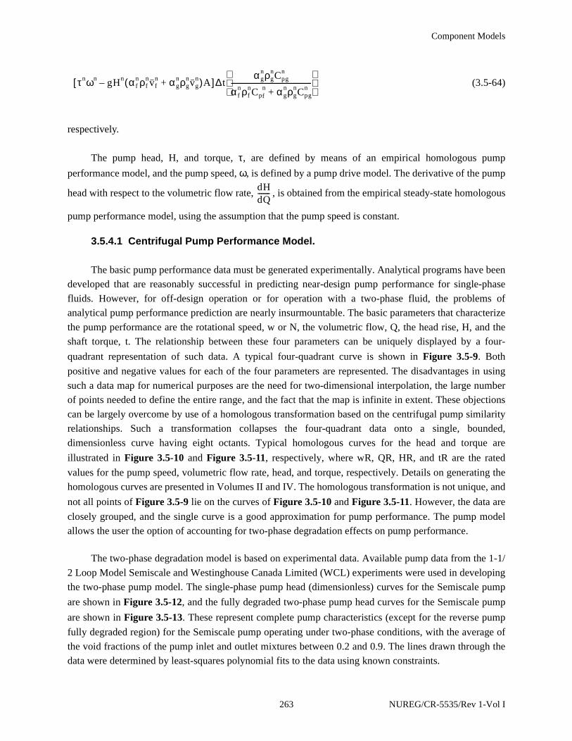
Component Models
(3.5-64)
respectively.
The pump head, H, and torque, τ, are defined by means of an empirical homologous pump
performance model, and the pump speed, ω, is defined by a pump drive model. The derivative of the pump
head with respect to the volumetric flow rate, , is obtained from the empirical steady-state homologous
pump performance model, using the assumption that the pump speed is constant.
3.5.4.1 Centrifugal Pump Performance Model.
The basic pump performance data must be generated experimentally. Analytical programs have been
developed that are reasonably successful in predicting near-design pump performance for single-phase
fluids. However, for off-design operation or for operation with a two-phase fluid, the problems of
analytical pump performance prediction are nearly insurmountable. The basic parameters that characterize
the pump performance are the rotational speed, w or N, the volumetric flow, Q, the head rise, H, and the
shaft torque, t. The relationship between these four parameters can be uniquely displayed by a four-
quadrant representation of such data. A typical four-quadrant curve is shown in Figure 3.5-9. Both
positive and negative values for each of the four parameters are represented. The disadvantages in using
such a data map for numerical purposes are the need for two-dimensional interpolation, the large number
of points needed to define the entire range, and the fact that the map is infinite in extent. These objections
can be largely overcome by use of a homologous transformation based on the centrifugal pump similarity
relationships. Such a transformation collapses the four-quadrant data onto a single, bounded,
dimensionless curve having eight octants. Typical homologous curves for the head and torque are
illustrated in Figure 3.5-10 and Figure 3.5-11, respectively, where wR, QR, HR, and tR are the rated
values for the pump speed, volumetric flow rate, head, and torque, respectively. Details on generating the
homologous curves are presented in Volumes II and IV. The homologous transformation is not unique, and
not all points of Figure 3.5-9 lie on the curves of Figure 3.5-10 and Figure 3.5-11. However, the data are
closely grouped, and the single curve is a good approximation for pump performance. The pump model
allows the user the option of accounting for two-phase degradation effects on pump performance.
The two-phase degradation model is based on experimental data. Available pump data from the 1-1/
2 Loop Model Semiscale and Westinghouse Canada Limited (WCL) experiments were used in developing
the two-phase pump model. The single-phase pump head (dimensionless) curves for the Semiscale pump
are shown in Figure 3.5-12, and the fully degraded two-phase pump head curves for the Semiscale pump
are shown in Figure 3.5-13. These represent complete pump characteristics (except for the reverse pump
fully degraded region) for the Semiscale pump operating under two-phase conditions, with the average of
the void fractions of the pump inlet and outlet mixtures between 0.2 and 0.9. The lines drawn through the
data were determined by least-squares polynomial fits to the data using known constraints.
τnωn gHn α fnρf
nvfn αg
nρgnvg
n+( )A–[ ]∆ tαg
nρgnCpg
n
α fnρf
nCpfn αg
nρgnCpg
n+-----------------------------------------------
dHdQ-------
263 NUREG/CR-5535/Rev 1-Vol I
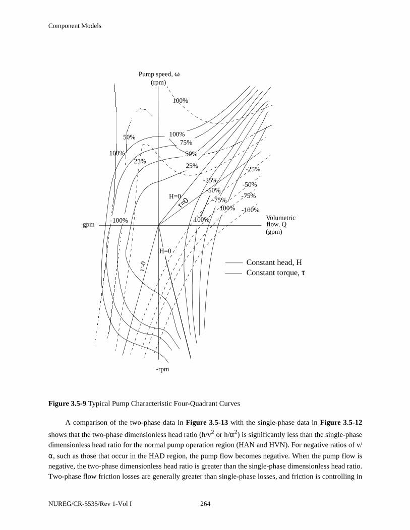
Component Models
A comparison of the two-phase data in Figure 3.5-13 with the single-phase data in Figure 3.5-12
shows that the two-phase dimensionless head ratio (h/v2 or h/α2) is significantly less than the single-phase
dimensionless head ratio for the normal pump operation region (HAN and HVN). For negative ratios of v/
α, such as those that occur in the HAD region, the pump flow becomes negative. When the pump flow is
negative, the two-phase dimensionless head ratio is greater than the single-phase dimensionless head ratio.
Two-phase flow friction losses are generally greater than single-phase losses, and friction is controlling in
Figure 3.5-9 Typical Pump Characteristic Four-Quadrant Curves
100%
100%75%
50%
25%
-25%
-50%
-75%-100%
100%
-100%
-75%
-50%
-25%
-100%
100%25%
50%
Volumetricflow, Q(gpm)
-gpm
Pump speed, ω(rpm)
H=0
H=0
τ=0
Constant head, HConstant torque, τ
-rpm
τ=0
NUREG/CR-5535/Rev 1-Vol I 264

Component Models
this energy dissipation region (HAD). The other regions of two-phase dimensionless head ratio data show
similar deviations from single-phase data.
Table 3.5-2 presents the difference between the single- and two-phase dimensionless head ratio data
as a function of v/α and α/v for the various pumping regions shown in Figure 3.5-12 and Figure 3.5-13where
Figure 3.5-10 Typical Pump Homologous Head Curves
h/α2 or h/v2
h/α2
v/α
h/α2
v/α
h/v2
h/v2
-1.0 1.0
α = ω/ωR (speed ratio)h = H/HR (head ratio)v = Q/QR (flow ratio)
α/vv/α or α/v
1.0
α/v
-1.0
0.0
265 NUREG/CR-5535/Rev 1-Vol I

Component Models
(3.5-65)
Figure 3.5-11 Typical Pump Homologous Torque Curves
β/α2 or β/v2
β/α2
v/α or α/v
-1.0
1.0
β/α2
1.0
α/v
β/v2
α = ω/ωR (speed ratio)
β/v2
v/α
v/α
β = τ/τR (torque ratio)
v = Q/QR (flow ratio)
-1.0
α/v
xvα--- or
αv---=
y h
α2-----
1φ
h
α2-----
2φ
–
or h
v2-----
1φ
h
v2-----
2φ
–
=
NUREG/CR-5535/Rev 1-Vol I 266

Component Models
The differences shown in Table 3.5-2 are for the eight curve types used for determining pump head.
Figure 3.5-12 Single-Phase Homologous Head Curves for 1-1/2 Loop MOD1 Semiscale Pumps
HAD(3)
HVD(4)
(7)
HAR
HVR
-0.5
(8)
1.5
1.0
0.5
0.0 0.5
-0.5
HAT(5)
HAN(1)
HVT(6)
HVN (2)
h/v2 or h/α2
h = H/HR head ratiov = Q/QR flow ratio
Normal pump
Energy dissipation
Normal turbine
Reverse pump
(+ Q, + α)
(- Q, + α)
(- Q, - α)
(+ Q, - α)
HANHVNHADHVDHATHVTHARHVR
{
{{
{
α/v or v/α
α = ω/ωR speed ratio
267 NUREG/CR-5535/Rev 1-Vol I
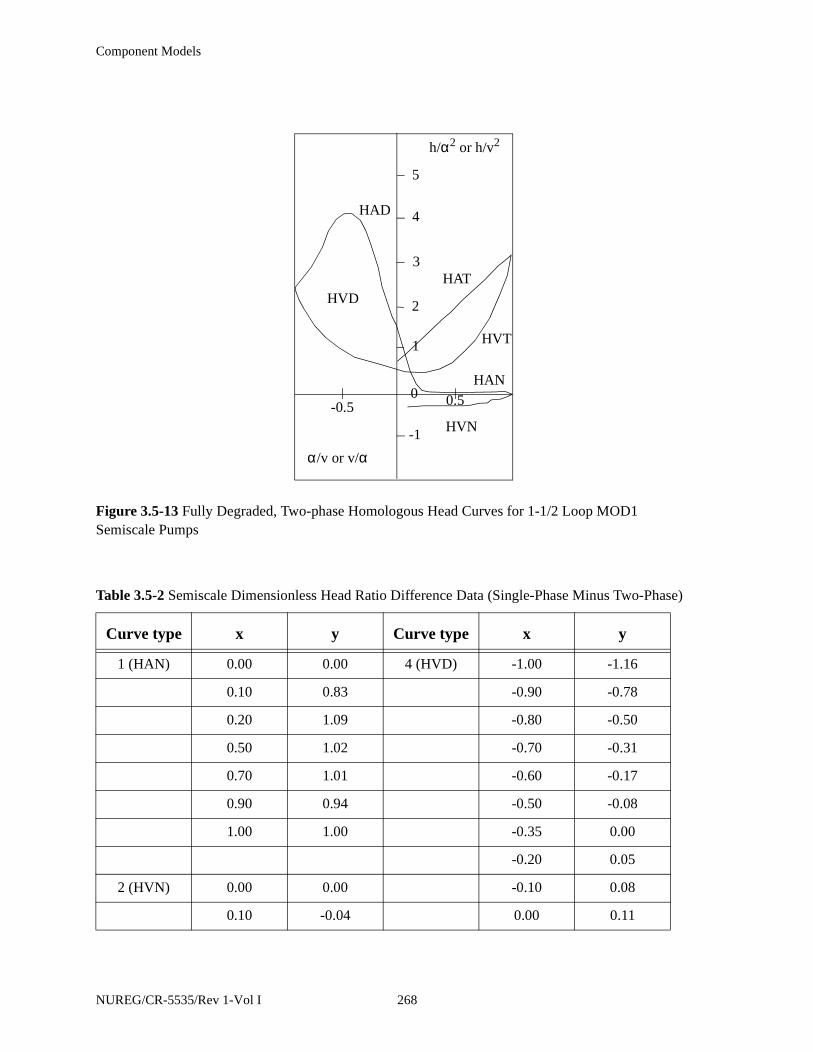
Component Models
Figure 3.5-13 Fully Degraded, Two-phase Homologous Head Curves for 1-1/2 Loop MOD1 Semiscale Pumps
Table 3.5-2 Semiscale Dimensionless Head Ratio Difference Data (Single-Phase Minus Two-Phase)
Curve type x y Curve type x y
1 (HAN) 0.00 0.00 4 (HVD) -1.00 -1.16
0.10 0.83 -0.90 -0.78
0.20 1.09 -0.80 -0.50
0.50 1.02 -0.70 -0.31
0.70 1.01 -0.60 -0.17
0.90 0.94 -0.50 -0.08
1.00 1.00 -0.35 0.00
-0.20 0.05
2 (HVN) 0.00 0.00 -0.10 0.08
0.10 -0.04 0.00 0.11
5
4
3
2
1
0
-1
HAT
HVT
HAN
HVN
HVD
-0.5 0.5
HAD
α/v or v/α
h/α2 or h/v2
NUREG/CR-5535/Rev 1-Vol I 268

Component Models
The head multiplier, MH(αg), and void fraction data shown in Table 3.5-3 were obtained in the
following manner. The Semiscale and WCL pump data3.5-6 were converted to dimensionless head ratios of
h/α2 or h/v2. Values of the dimensionless head ratios were obtained for pump speeds and volumetric flow
rates within 50% of the rated speed and flow rate for the pumps. The difference between the single- and
two-phase dimensionless ratios was developed as a function of the average void fractions for the pump
0.20 0.00
0.30 0.10 5 (HAT) 0.00 0.00
0.40 0.21 0.20 -0.34
0.80 0.67 0.40 -0.65
0.90 0.80 0.60 -0.95
1.00 1.00 0.80 -1.19
1.00 -1.47
3 (HAD) -1.00 -1.16
-0.90 -1.24 6 (HVT) 0.00 0.11
-0.80 -1.77 0.10 0.13
-0.70 -2.36 0.25 0.15
-0.60 -2.79 0.40 0.13
-0.50 -2.91 0.50 0.07
-0.40 -2.67 0.60 -0.04
-0.25 -1.69 0.70 -0.23
-0.10 -0.50 0.80 -0.51
0.00 0.00 0.90 -0.91
1.00 -1.47
7 (HAR) -1.00 0.00
0.00 0.00
8 (HVR) -1.00 0.00
0.00 0.00
Table 3.5-2 Semiscale Dimensionless Head Ratio Difference Data (Single-Phase Minus Two-Phase)
Curve type x y Curve type x y
269 NUREG/CR-5535/Rev 1-Vol I

Component Models
inlet and outlet mixtures. The difference between the single- and two-phase dimensionless ratios was then
normalized to a value between 0 and 1.0. The normalized result was tabulated as a function of the void
fraction.
If the two-phase option is selected, the pump head and torque are calculated from
H = H1φ - MH(αg) (H1φ - H2φ) (3.5-66)
τ = τ1φ - Mτ(αg) (τ1φ - τ2φ) (3.5-67)
where
1φ = single-phase value
2φ = two-phase, fully degraded value, 0.2 < αg < 0.9
M = multiplier on difference curve as a function of αg
Assumptions inherent in the pump model for two-phase flow include:
• The head multiplier, MH(αg), determined empirically for the normal operating region of
the pump, is also valid as an interpolating factor in all other operating regions.
• The relationship of the two-phase to the single-phase behavior of the Semiscale pump isapplicable to large reactor pumps. This assumes that the pump model of two-phase flowis independent of pump specific speed.
Table 3.5-3 Head Multiplier and Void Fraction Data
αg MH(αg)
0.000 0.00
0.070 0.00
0.080 0.74
0.165 1.00
0.900 1.00
1.000 0.00
NUREG/CR-5535/Rev 1-Vol I 270
Component Models
3.5.4.2 Centrifugal Pump Drive Model.
The pump torque is used to calculate the pump speed after the pump has been shut off by the input
trip signal. The speed is calculated by the deceleration equation
(3.5-68)
The finite difference approximation of this equation is
(3.5-69)
where
τ = net torque
I = moment of inertia
t = time
∆t = time step
ω = angular velocity
The rate of energy addition to the pump system is given by τω and has been used in Equation (3.5-
62) to calculate the pump dissipation.
The total pump torque is calculated by considering the hydraulic torque from the homologous curves
and the pump frictional torque. The net torque with the drive motor shut off is
τ = τhy + τfr (3.5-70)
where
τhy = hydraulic torque
τfr = frictional torque
The frictional torque is in the form of a cubic equation. The value of the frictional torque is also
dependent on the sign of the pump speed. An option is available to specify whether reverse rotation of the
pump is allowed.
Idωdt------- τ=
ωt ∆t+ ωtτ∆ t
I--------+=
271 NUREG/CR-5535/Rev 1-Vol I
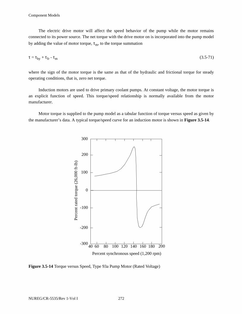
Component Models
The electric drive motor will affect the speed behavior of the pump while the motor remains
connected to its power source. The net torque with the drive motor on is incorporated into the pump model
by adding the value of motor torque, τm, to the torque summation
τ = τhy + τfr - τm (3.5-71)
where the sign of the motor torque is the same as that of the hydraulic and frictional torque for steady
operating conditions, that is, zero net torque.
Induction motors are used to drive primary coolant pumps. At constant voltage, the motor torque is
an explicit function of speed. This torque/speed relationship is normally available from the motor
manufacturer.
Motor torque is supplied to the pump model as a tabular function of torque versus speed as given by
the manufacturer’s data. A typical torque/speed curve for an induction motor is shown in Figure 3.5-14.
Figure 3.5-14 Torque versus Speed, Type 93a Pump Motor (Rated Voltage)
40 60 80 100 120 160 180 200140
Percent synchronous speed (1,200 rpm)
Per
cent
rat
ed to
rque
(26
,000
ft-
lb)
300
200
100
0
-100
-200
-300
NUREG/CR-5535/Rev 1-Vol I 272
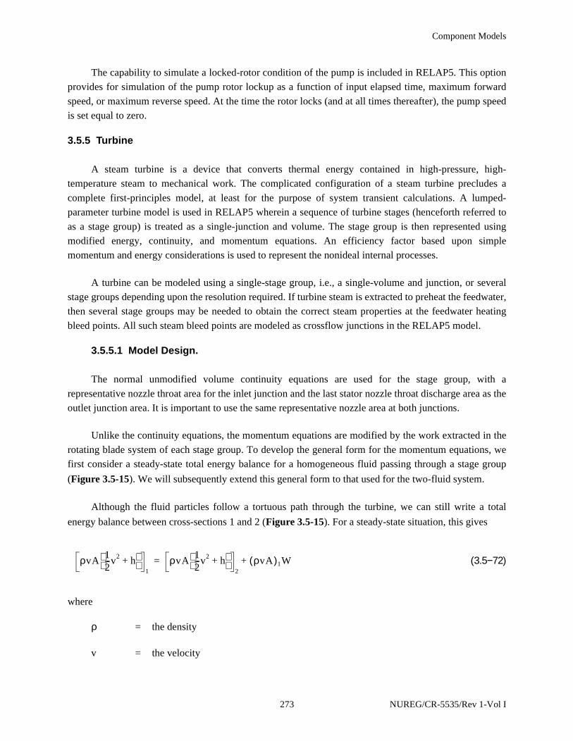
Component Models
The capability to simulate a locked-rotor condition of the pump is included in RELAP5. This option
provides for simulation of the pump rotor lockup as a function of input elapsed time, maximum forward
speed, or maximum reverse speed. At the time the rotor locks (and at all times thereafter), the pump speed
is set equal to zero.
3.5.5 Turbine
A steam turbine is a device that converts thermal energy contained in high-pressure, high-
temperature steam to mechanical work. The complicated configuration of a steam turbine precludes a
complete first-principles model, at least for the purpose of system transient calculations. A lumped-
parameter turbine model is used in RELAP5 wherein a sequence of turbine stages (henceforth referred to
as a stage group) is treated as a single-junction and volume. The stage group is then represented using
modified energy, continuity, and momentum equations. An efficiency factor based upon simple
momentum and energy considerations is used to represent the nonideal internal processes.
A turbine can be modeled using a single-stage group, i.e., a single-volume and junction, or several
stage groups depending upon the resolution required. If turbine steam is extracted to preheat the feedwater,
then several stage groups may be needed to obtain the correct steam properties at the feedwater heating
bleed points. All such steam bleed points are modeled as crossflow junctions in the RELAP5 model.
3.5.5.1 Model Design.
The normal unmodified volume continuity equations are used for the stage group, with a
representative nozzle throat area for the inlet junction and the last stator nozzle throat discharge area as the
outlet junction area. It is important to use the same representative nozzle area at both junctions.
Unlike the continuity equations, the momentum equations are modified by the work extracted in the
rotating blade system of each stage group. To develop the general form for the momentum equations, we
first consider a steady-state total energy balance for a homogeneous fluid passing through a stage group
(Figure 3.5-15). We will subsequently extend this general form to that used for the two-fluid system.
Although the fluid particles follow a tortuous path through the turbine, we can still write a total
energy balance between cross-sections 1 and 2 (Figure 3.5-15). For a steady-state situation, this gives
(3.5−72)
where
ρ = the density
v = the velocity
ρvA12---v2 h+
1
ρvA12---v2 h+
2
ρvA( )1W+=
273 NUREG/CR-5535/Rev 1-Vol I
Component Models
h = the enthalpy
A = the cross-sectional area
The term W represents the shaft work per mass flow rate extracted from the fluid. Heat loss is
neglected in this ideal analysis. From continuity considerations, ρvA is constant. Dividing Equation (3.5-
72) by ρvA, we obtain
(3.5-73)
In this way, the energy balance is converted into an equivalent force balance (power = force x
velocity).
In this idealized process where external heat loss and internal dissipation are neglected, the process is
isentropic and
(3.5-74)
Integrating Equation (3.5-74) approximately (assuming constant density) between points 1 and 2
gives
Figure 3.5-15 A Schematic of a Stage Group with Idealized Flow Path between Points 1 and 2
1
2
Fixedblades
Moving blades
12---v2
2 12---v1
2– h2 h1–( )– W–=
dh1ρ---dP=
NUREG/CR-5535/Rev 1-Vol I 274
Component Models
(3.5-75)
where ρ is an average density.
The actual work, W, produced by the fluid on the rotating blades as its momentum is changed, is
usually written as an efficiency factor times the isentropic enthalpy change across the stage and becomes
(3.5-76)
If a constant efficiency and density for the stage group is assumed, Equation (3.5-76) can be
approximated as
(3.5-77)
When Equation (3.5-75) and (3.5-77) are substituted into Equation (3.5-73), we obtain
(3.5-78)
as the momentum equation for this steady-state case. Equation (3.5-78) shows that only a small fraction, (1
- η), of the pressure gradient contributes to changes in the kinetic energy of the fluid. The larger fraction,
η, of the pressure gradient results in turbine work [Equation (3.5-77)].
Using Equation (3.5-78) as a prototype, the full two-fluid momentum equations which are used in the
turbine model are (in differential form)
(3.5-79)
(3.5-80)
The application guidelines will be summarized in Volume II of this report, but it seems appropriate at
this point to mention three guidelines that are related to the momentum equation development:
h2 h1–1ρ--- P2 P1–( )=
W η dhS const=
∫– η 1ρ---dP
S const=
∫–= =
W η 1ρ--- P2 P1–( )–=
12---v2
2 12---v1
2–1 η–( )
ρ----------------- P2 P1–( )–=
α gρg( )∂vg
∂t-------- vg
∂vg
∂x--------+
αg 1 η–( )∂P∂x------– αgρgHLOSSG vg– αgρg FIG vg vf–( )–=
α fρf( )∂vf
∂t------- vf
∂vf
∂x-------+
α f 1 η–( )∂P∂x------– α fρfHLOSSF vf– α fρf FIF vf vg–( )–=
275 NUREG/CR-5535/Rev 1-Vol I

Component Models
1. In practice, a steam turbine does not usually contain significant liquid water, and thetortuous path precludes accurate modeling of the interphase drag. Therefore, it isrecommended that the homogeneous option be used at all axial turbine junctions. Theeffect of condensation could be included in the efficiency factor, if desired. At present,it is not included, as the effect is usually small.
2. The fluid path through the turbine volume is very tortuous. This, coupled with thelarge number of blades, makes the standard wall friction calculation meaningless. Forthis reason, the wall friction terms have not been shown in Equation (3.5-79) and (3.5-80). It is recommended that the turbine volume wall friction flag be set to use the zerowall friction option. If the user wants to include any momentum effects due tofrictional or form losses, it should be done with an appropriate user-specified formloss.
3. The area changes in a turbine are gradual, so the smooth junction option should beused.
The inefficiency of the turbine gives rise to some dissipation that is a source of internal energy. The
dissipation is assumed to be a small effect and is neglected in the present turbine model formulation.
The only equations that are modified as a result of the turbine model are the momentum equations, in
which the pressure gradient terms are multiplied by the coefficient (1 - η).
3.5.5.2 Efficiency Formulas.
The basic efficiency formulas can be derived from velocity diagrams with assumed nozzle and blade
efficiency factors. The derivations are fairly straightforward and are found in standard texts. The efficiency
formulas recorded here were obtained from Reference 3.5-7. The efficiency factors for three turbine
designs are described in the following paragraph.
3.5.5.2.1 Single-Stage Turbine
The first model considered is the most general. We consider a single-row fixed-blade system
followed by a single-row rotating-blade system. Let r be the reaction fraction, i.e., the fraction of the stage
energy released (enthalpy change) in the moving-blade system. If r is zero, we have a pure impulse stage
with no pressure drop in the moving-blade system, i.e., the moving blades only change the fluid flow
direction. A turbine stage with nonzero r at design conditions is commonly called a reaction stage. A value
of r = 0.5 is a common design.
If all blading angles are ideal and all nozzle losses are zero, the ideal efficiency, as given in
Reference 3.5-7, is
NUREG/CR-5535/Rev 1-Vol I 276
Component Models
(3.5−81)
where v is the fluid velocity at the nozzle exit, vt is the tangential or rim velocity of the moving blades, and
b = (1 - r)1/2 (3.5-82)
In general, due to nozzle losses, entrance effects, and nonideal blading angles, the efficiency is less
than that given by Equation (3.5-81). The maximum efficiency (η = 1.0) given by Equation (3.5-81) can be
found by differentiation to occur when
(3.5-83)
For an impulse stage, the maximum efficiency occurs at . For a reaction turbine designed
with r = 0.5, the maximum efficiency occurs at .
In general, the actual efficiency is less than the ideal value derived above. A first approximation to
the actual efficiency (see Reference 3.5-7) is to include a constant factor, ηo, in Equation (3.5-81) that
represents the actual efficiency at the maximum point, i.e.,
(3.5−84)
Equation (3.5-84) is the general efficiency formula that is applied to a single-row impulse or reaction
turbine. This formula is applied to a stage group that may consist of a single-blade passage or multiple-
blade passages. If the stage group contains multiple-blade passages, the efficiency represents some average
value.
3.5.5.2.2 Two-Stage Impulse Turbine
The second turbine design considered is a two-row impulse stage, i.e., a nozzle, a moving constant-
area blade passage, a fixed constant-area stationary passage, and a final constant-area moving blade
passage. This blading system is modeled as a single-stage group. This type of stage design is sometimes
used as the first stage in a turbine for governing purposes. Reference 3.5-7 records the efficiency formula
for this design as
η vb vt–( ) vb vt–( )2 rv2+[ ] 1 2⁄+{ }
2vt
v2-------
=
vt
v----
0.5
1 r–( )1 2⁄----------------------=
vt
v---- 0.50=
vt
v---- 0.707=
η η o
2vt
v2------- vb vt–( ) vb vt–( )2 rv2+[ ] 1 2⁄
+{ }=
277 NUREG/CR-5535/Rev 1-Vol I

Component Models
(3.5-85)
3.5.5.2.3 Constant Efficiency
The final efficiency option that is included is a constant efficiency independent of the reaction,
nozzle fluid velocity, and rim speed, i.e.,
η = ηo (3.5-86)
It should be noted that a turbine stage, designed to operate with a given reaction fraction r at design
conditions, will have a different reaction fraction for off-design conditions. The change in reaction fraction
with can be calculated [Reference 3.5-7, p. 207, Equation (14)]. For reaction stages, the change is
small. In all cases, this change in r is neglected in the above efficiency formulas.
3.5.5.2.4 Power/Torque Output of Turbine
In general, the relationship between power and torque for a rotating shaft is
P = τω (3.5-87)
The power extracted from the fluid per mass flow rate for a given stage group is
(3.5-88)
so we have for the torque
(3.5-89)
or
(3.5−90)
where R is the mean stage radius at the nozzle and the approximation in Equation (3.5-77) has been used.
η η o
8vt
v2------- v 2vt–( )=
vt
v----
η hdS= const
∫
τ ρvA( )ηρ---
P2 P1–( )ω
---------------------=
τ ρvA( )ηρ--- P2 P1–( )R
vt----=
NUREG/CR-5535/Rev 1-Vol I 278
Component Models
Equation (3.5-90) gives the torque that is extracted from a given stage group in terms of the stage
efficiency, mean stage radius R, mean blade tangential velocity vt, and pressure drop. This is the torque
that is applied by the turbine component when it is coupled to the shaft component.
3.5.5.2.5 Numerical Implementation
As noted in the model design section, a stage group is modeled as a single-junction (j) and volume
(L) (see Figure 3.5-16).
The continuity and internal energy equations in Section 3.1 are unchanged from their standard form.
The normal finite difference form of the momentum equations for junction j is modified in two ways:
1. The pressure gradient term in the sum and difference numerical equations ismultiplied by (1 - η).
2. The numerical differencing of the convective terms has been modified. At a normaljunction, the convective terms are approximated as
(3.5-91)
The small viscous term VIS is numerically calculated so as to give a donored formulation of the
momentum flux term in a straight pipe. For a variable-area channel, it is formulated so that it vanishes for
a variable-area channel with a constant density fluid. In a turbine, the area is slowly varying; but the fluid
experiences large pressure changes (due to the work extraction), hence large density changes. A numerical
simulation with the above convective terms used at the turbine junctions resulted in a viscous term that is
larger than the kinetic energy terms. The normal viscous terms for a variable area channel are inaccurate in
the turbine situation with large density changes and dominate the physical kinetic energy change. An
alternative form of the convective terms which is sufficiently accurate and stable for the variable area
turbine model is
(3.5-92)
when the flow is from left to right in Figure 3.5-16.
This difference form is used for all turbine junctions. If the vj multiplying the numerical gradient is
assumed to be approximately equal to , then Equation (3.5-92) yields
v∂v∂x------
12---vL
2 12---vK
2–
∆x------------------------
12---
VIS∆x
----------+=
v∂v∂x------
vj vj vj 1––( )∆x
-----------------------------=
12--- vj vj 1–+( )
279 NUREG/CR-5535/Rev 1-Vol I
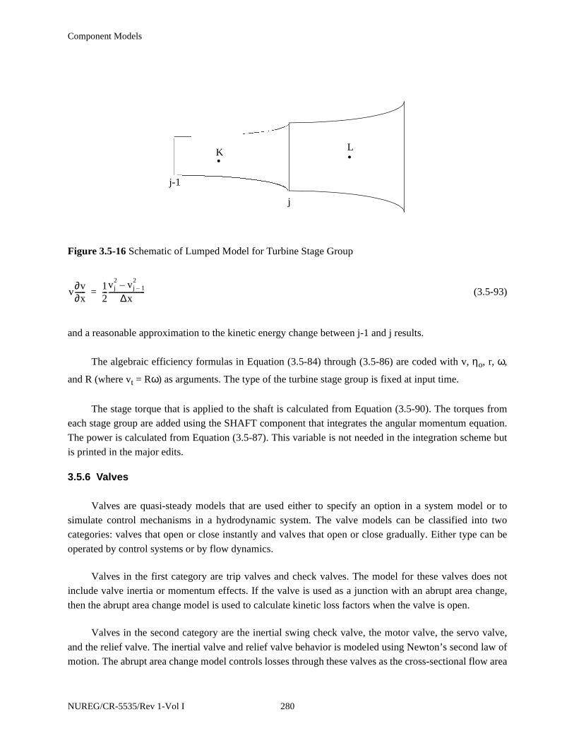
Component Models
(3.5-93)
and a reasonable approximation to the kinetic energy change between j-1 and j results.
The algebraic efficiency formulas in Equation (3.5-84) through (3.5-86) are coded with v, ηo, r, ω,
and R (where vt = Rω) as arguments. The type of the turbine stage group is fixed at input time.
The stage torque that is applied to the shaft is calculated from Equation (3.5-90). The torques from
each stage group are added using the SHAFT component that integrates the angular momentum equation.
The power is calculated from Equation (3.5-87). This variable is not needed in the integration scheme but
is printed in the major edits.
3.5.6 Valves
Valves are quasi-steady models that are used either to specify an option in a system model or to
simulate control mechanisms in a hydrodynamic system. The valve models can be classified into two
categories: valves that open or close instantly and valves that open or close gradually. Either type can be
operated by control systems or by flow dynamics.
Valves in the first category are trip valves and check valves. The model for these valves does not
include valve inertia or momentum effects. If the valve is used as a junction with an abrupt area change,
then the abrupt area change model is used to calculate kinetic loss factors when the valve is open.
Valves in the second category are the inertial swing check valve, the motor valve, the servo valve,
and the relief valve. The inertial valve and relief valve behavior is modeled using Newton’s second law of
motion. The abrupt area change model controls losses through these valves as the cross-sectional flow area
Figure 3.5-16 Schematic of Lumped Model for Turbine Stage Group
• •K L
j-1
j
v∂v∂x------
12---
vj2 vj 1–
2–∆x
---------------------=
NUREG/CR-5535/Rev 1-Vol I 280

Component Models
varies with valve assembly movement. The motor and servo valve use differential equations to control
valve movement. These two valves include the options to use the abrupt area change model to calculate
losses across the valve or to use flow coefficients (Cv) specified by the user. The Cv’s are converted to
energy loss coefficients within the numerical scheme [see Equation (3.5-107)].
Valves are modeled as junction components. The types of valves are defined as follows.
3.5.6.1 Trip Valve.
The operation of a trip valve is solely dependent on the trip selected. With an appropriate trip, an
abrupt full opening or full closing of the valve will occur. A latch option is also included for latching the
valve in the open or closed position.
3.5.6.2 Check Valve.
The operation of a check valve can be specified to open or close by static differential pressure, to
open by static differential pressure and close by flow reversal, or to open by static differential pressure and
close by dynamic differential pressure.
All of the check valves will be opened based on static differential pressure across the junction
according to
- PCV > 0, valve opens (3.5-94)
where
PK, PL = junction from and to volume thermodynamic pressures
= static pressure head due to gravity
PCV = back pressure required to close the valve (user input)
For a static pressure controlled check valve, the valve will open if Equation (3.5-94) becomes
positive and will close if Equation (3.5-94) becomes negative. If Equation (3.5-94) is zero, the valve will
remain as previously defined.
For a flow controlled check valve, the valve will open if Equation (3.5-94) is positive and will close
only if a flow reversal occurs such that
GC < 0 (3.5-95)
PK ∆PKg–( ) PL ∆PLg
+( )–
∆PKg∆PLg
,
281 NUREG/CR-5535/Rev 1-Vol I
Component Models
where GC is the dynamic pressure given as
(3.5-96)
For a dynamic pressure controlled check valve, the valve opens if Equation (3.5-94) is greater than
zero. Once the valve is open, the forces due to pressure differential and momentum hold the valve open
until
+ GC - PCV < 0, valve closes, (3.5-97)
= 0, remains as previously defined.
The terms αf and αg are the junction liquid and vapor volume fractions, respectively; ρf and ρg are
the junction liquid and vapor densities, respectively; and vf and vg are the junction liquid and vapor
velocities, respectively.
Flow and dynamic pressure controlled valves exhibit a hysteresis effect with respect to the forces
opening and closing the valve. The static pressure controlled valve, however, has no hysteresis effect.
All check valves may be initialized as either open or closed. Leakage is also allowed if the valve is
closed, and the abrupt area change model is used to calculate the valve form losses.
3.5.6.3 Inertial Valve.
This valve models the motion of the valve flapper assembly in an inertial-type check valve. The
abrupt area change model is used to calculate kinetic form losses, assuming that the area between the
flapper and the valve seat behaves as an orifice whose area changes in time as a function of the inertial
valve geometry.
The motion of the flapper about the shaft axis is given by Newton’s second law (angular version) as
(3.5-98)
where
T = torque
I = moment of inertia
GC12--- ρv v( )j
12--- α fρfvf vf α gρgvg vg+( )j= =
PK ∆PKg–( ) PL ∆PLg
+( )–
ΣT Iω·=
NUREG/CR-5535/Rev 1-Vol I 282

Component Models
= angular acceleration
ω = angular velocity = , counter-clockwise motion is positive
θ = disc angular position, θ = 0 is fully closed
Torque is defined as r x F; the cross-product of a force F and the distance from the hinge pivot point,
r, to the force. Each particle of a rotating body has kinetic energy. Kinetic energy is defined as 0.5mV2
where m is the mass and V is the velocity. Since V = rω where r is the distance to the particle and ω is the
angular velocity, the kinetic energy of the particle is 0.5mr2ω2. The total kinetic energy of a rotating body
is the sum of the kinetic energy of all of its particles. Since the angular velocity of all particles is the same,
ω can be factored out to give:
(3.5-99)
The term in parentheses is know as the moment of inertia, I.
A diagram of an inertial valve is shown in Figure 3.5-17. The valve flapper disc resides in a pipe and
swings on a hinge pin. The valve are used to prevent backflow. The flapper position depends on factors
such as: flapper mass, gravity vector, moment of inertia, distance from the hinge pin to the center of mass,
flapper area, pressure difference across the valve, viscous and Coulomb friction between the flapper and
the pin and lift and drag forces on the flapper. Only torque due to differential pressure, TDP, Coulomb
friction, TF, and weight, TW, are included in this model:
TDP = (PK - PL) APL (3.5-100)
TF = ∆PFARL (3.5-101)
TW = -MgLsinθ (3.5-102)
where
PK = pressure in the hydraulic cell on the left
PL = pressure in the hydraulic cell on the right
Ap = projected area of the disc
L = user input flapper moment arm length from the hinge to the center of inertia
ω·
θ·
Kinetic Energy 0.5 Σmiri2( )ω2=
283 NUREG/CR-5535/Rev 1-Vol I
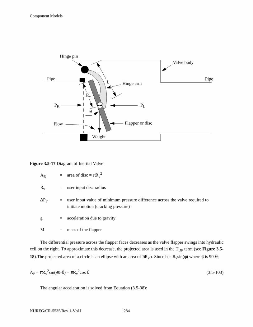
Component Models
AR = area of disc = πRv2
Rv = user input disc radius
∆PF = user input value of minimum pressure difference across the valve required to
initiate motion (cracking pressure)
g = acceleration due to gravity
M = mass of the flapper
The differential pressure across the flapper faces decreases as the valve flapper swings into hydraulic
cell on the right. To approximate this decrease, the projected area is used in the TDP term (see Figure 3.5-
18).The projected area of a circle is an ellipse with an area of πRvb. Since b = Rvsin(φ) where φ is 90-θ;
AP = πRv2sin(90-θ) = πRv
2cos θ (3.5-103)
The angular acceleration is solved from Equation (3.5-98):
Figure 3.5-17 Diagram of Inertial Valve
L
Weight
Pipe
PK PL
Hinge pin
Flow
Rv
θ
Hinge arm
Flapper or disc
Valve body
Pipe
NUREG/CR-5535/Rev 1-Vol I 284

Component Models
(3.5-104)
and the new time flapper velocity and angle are:
(3.5-105)
The new time angle is calculated from the angle at the previous time step and the average velocity
during the time step.
θn = θn - 1 + 0.5(ωn - 1 + ωn) ∆t (3.5-106)
where superscript n stands for new time and n-1 indicates the previous time step value.
In order to obtain the correct velocity to compare with the sonic speed at the valve the vena-contracta
is considered. The effective flow area is Cc times the actual open area, where,
Cc = contraction coefficient, effective area/actual open area.
Table 3.5-4 gives the table of contraction coefficients.3.5-8 Cc is less than one and has the effect of
increasing the code calculated velocity in the valve opening. Also shown is the loss coefficient which the
abrupt area change model automatically calculates for the code users. Volume IV discusses this in more
detail.
.
Figure 3.5-18 Two Views of a Partially Open Flapper Valve
Rvb
Front view Side view
Θ
bφ
Rv
ω· n ΣTI
-------=
ωn ωn 1– ω· n∆t+=
285 NUREG/CR-5535/Rev 1-Vol I
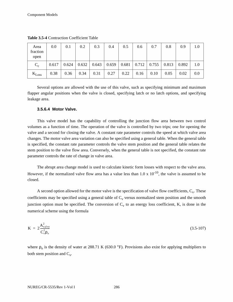
Component Models
Several options are allowed with the use of this valve, such as specifying minimum and maximum
flapper angular positions when the valve is closed, specifying latch or no latch options, and specifying
leakage area.
3.5.6.4 Motor Valve.
This valve model has the capability of controlling the junction flow area between two control
volumes as a function of time. The operation of the valve is controlled by two trips; one for opening the
valve and a second for closing the valve. A constant rate parameter controls the speed at which valve area
changes. The motor valve area variation can also be specified using a general table. When the general table
is specified, the constant rate parameter controls the valve stem position and the general table relates the
stem position to the valve flow area. Conversely, when the general table is not specified, the constant rate
parameter controls the rate of change in valve area.
The abrupt area change model is used to calculate kinetic form losses with respect to the valve area.
However, if the normalized valve flow area has a value less than 1.0 x 10⁻¹⁰, the valve is assumed to be
closed.
A second option allowed for the motor valve is the specification of valve flow coefficients, Cv. These
coefficients may be specified using a general table of Cv versus normalized stem position and the smooth
junction option must be specified. The conversion of Cv to an energy loss coefficient, K, is done in the
numerical scheme using the formula
(3.5-107)
where ρo is the density of water at 288.71 K (630.0 °F). Provisions also exist for applying multipliers to
both stem position and Cv.
Table 3.5-4 Contraction Coefficient Table
Area fraction
open
0.0 0.1 0.2 0.3 0.4 0.5 0.6 0.7 0.8 0.9 1.0
Cc 0.617 0.624 0.632 0.643 0.659 0.681 0.712 0.755 0.813 0.892 1.0
KLoss 0.38 0.36 0.34 0.31 0.27 0.22 0.16 0.10 0.05 0.02 0.0
K 2Avalve
2
Cv2ρo
--------------=
NUREG/CR-5535/Rev 1-Vol I 286
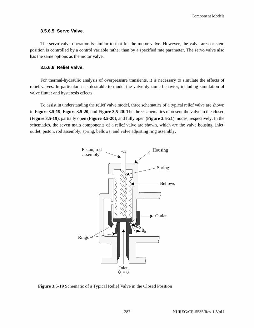
Component Models
3.5.6.5 Servo Valve.
The servo valve operation is similar to that for the motor valve. However, the valve area or stem
position is controlled by a control variable rather than by a specified rate parameter. The servo valve also
has the same options as the motor valve.
3.5.6.6 Relief Valve.
For thermal-hydraulic analysis of overpressure transients, it is necessary to simulate the effects of
relief valves. In particular, it is desirable to model the valve dynamic behavior, including simulation of
valve flutter and hysteresis effects.
To assist in understanding the relief valve model, three schematics of a typical relief valve are shown
in Figure 3.5-19, Figure 3.5-20, and Figure 3.5-20. The three schematics represent the valve in the closed
(Figure 3.5-19), partially open (Figure 3.5-20), and fully open (Figure 3.5-21) modes, respectively. In the
schematics, the seven main components of a relief valve are shown, which are the valve housing, inlet,
outlet, piston, rod assembly, spring, bellows, and valve adjusting ring assembly.
HousingPiston, rodassembly
Outlet
Inlet
Spring
Bellows
α0θ0
θi = 0
Rings
Figure 3.5-19 Schematic of a Typical Relief Valve in the Closed Position
287 NUREG/CR-5535/Rev 1-Vol I

Component Models
The numerical model of the valve simply approximates the fluid forces acting on the valve piston and
the valve reaction to these forces. The model of the fluid forces is based on a quasi-steady-state form of the
impulse momentum principle, and the valve reaction force is based on Newton’s Second Law of motion.
A qualitative understanding of the operation of the relief valve can be gained by referring again to
Figure 3.5-19, Figure 3.5-20, and Figure 3.5-20. If the valve inlet pressure is low the valve is closed, as
shown in Figure 3.5-19. As the inlet pressure increases, the valve piston will remain closed until the force
of the upstream pressure on the valve exceeds the set point forces. The set point forces are the combined
forces of the piston and rod assembly weight, the valve spring, the atmospheric pressure inside the bellows,
and the downstream back pressure around the outside of the bellows. Once the set point forces are
exceeded, the valve piston will begin to lift. Upon opening, the upstream fluid will begin to expand
through the opening into the valve ring region. This initial expansion occurs through the angle αo, and the
flow changes direction through an average angle θo, as shown in Figure 3.5-19. As the flow accelerates,
the momentum effects of the expansion and change in flow direction exert a thrust on the valve piston,
causing the valve to open further. As the valve partially opens, the angle of expansion decreases to α1 and
the change in flow direction increases to θ1, as shown in Figure 3.5-20. This effect, in turn, further
DB, ABa
Pi, vi, DD, AD
ABo = (Ap - ABa)
Dp, Ap
Vv
vi
θ1, Pe, ve, Ae
α1
Pa
Po
Pe, Ae
X1
Figure 3.5-20 Schematic of a Typical Relief Valve in the Partially Open Position
NUREG/CR-5535/Rev 1-Vol I 288

Component Models
increases the thrust on the valve piston, causing it to fully open, as shown in Figure 3.5-21. As these
processes occur, the valve reaction forces and fluid momentum forces vary in such a manner that the valve
will not close until the upstream pressure decreases significantly below the valve set point pressure. In this
respect, a hysteresis effect is observed that is characteristic of relief valves.
The relief valve model consists of a set of equations designed to approximate the behavior described
above. In implementing the model, the dynamic behavior of the fluid is calculated at each time step by the
RELAP5 hydrodynamic solution scheme. The resultant phasic velocities and thermodynamic properties
are then used to solve a quasi-steady equation approximating the fluid forces on the valve piston. The valve
dynamic reaction forces are then calculated, and the new time valve piston speed and position are
estimated.
The relief valve model is formulated, applying D’Alembert’s principle in which the forces acting on
the face of the valve piston are balanced, for which the valve reaction forces can be written as
(reaction forces) = FR = mvav,x + B (vv,x - vhousing) + Ksx (3.5-108)
where
Do Ds
Di
Ho Hi
Figure 3.5-21 Schematic of a Typical Relief Valve in the Fully Open Position
289 NUREG/CR-5535/Rev 1-Vol I

Component Models
mv = mass of the valve mechanism that is in motion (i.e. the valve piston, rod
assembly combined with the spring and bellows)
av,x = valve assembly acceleration in the x-direction
B = damping coefficient
vv,x = velocity of the valve mechanism in the x-direction
vhousing = velocity of the valve housing = 0
Ks = spring constant
x = piston position (i.e., x-coordinate)
NUREG/CR-5535/Rev 1-Vol I 290

Component Models
The positive x-direction is assumed to be in the direction of fluid flow at the valve inlet. The fluid
forces, FF, can be formulated by summing the forces acting over the surfaces of the fluid flow channel such
that
FF = (PiAD)x - (PaABa)x - (PoABo) - (PeAe)x - FR (3.5-109)
where
FR = reaction forces
Pi = valve inlet pressure
AD = valve piston face area exposed to the inlet flow stream
Pa = atmospheric pressure inside the bellows
ABa = valve piston area inside the bellows
Po = valve back pressure outside the bellows
ABo = valve piston area outside the bellows
Ae = valve ring exit area
Pe = valve ring exit pressure
and where the subscript x denotes that the force component is in the x-direction. Since the fluid is flowing
through a channel that both expands and changes direction, the fluid undergoes a change in momentum
expressed by the impulse momentum principle as
(3.5-110)
where
= mass flow rate of the fluid through the valve
ve,x = fluid velocity exiting through the rings
vi,x = fluid velocity entering the valve inlet
Balancing the forces by combining Equation (3.5-108) through (3.5-110) gives
FF ∆ mv( ) m· F ve x, vi x,–( )= =
m· F
291 NUREG/CR-5535/Rev 1-Vol I
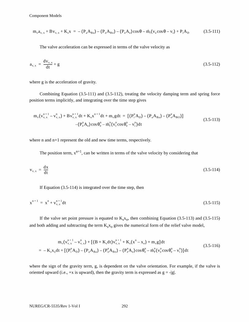
Component Models
(3.5-111)
The valve acceleration can be expressed in terms of the valve velocity as
(3.5-112)
where g is the acceleration of gravity.
Combining Equation (3.5-111) and (3.5-112), treating the velocity damping term and spring force
position terms implicitly, and integrating over the time step gives
(3.5-113)
where n and n+1 represent the old and new time terms, respectively.
The position term, xn+1, can be written in terms of the valve velocity by considering that
(3.5-114)
If Equation (3.5-114) is integrated over the time step, then
(3.5-115)
If the valve set point pressure is equated to Ksxo, then combining Equation (3.5-113) and (3.5-115)
and both adding and subtracting the term Ksxo gives the numerical form of the relief valve model,
(3.5-116)
where the sign of the gravity term, g, is dependent on the valve orientation. For example, if the valve is
oriented upward (i.e., +x is upward), then the gravity term is expressed as g = -|g|.
mvav x, Bvv x, Ksx+ + PaABa( )– PoABo( )– PeAe( ) θ m· f ve θ vi–cos( )– PiAD+cos–=
av x,dvv x,
dt------------ g+=
mv vv x,n 1+ vv x,
n–( ) Bvv x,n 1+ dt Ksx
n 1+ dt mvgdt+ + + PinAD( ) PaABa( )– Po
nABO( )–[ ]=
PenAe( ) θe
n m· fn vc
n θen vi
n–cos( )dt–cos–
vv x,dxdt------=
xn 1+ xn vv x,n 1+ dt+=
mv vv x,n 1+ vv x,
n–( ) B Ksdt+( )vv x,n 1+ Ks xn xo–( ) mvg+ +[ ] dt+
Ksxodt– PinAD( ) PaABa( )– Po
nABo( )– PenAe( ) θe
n m· Fn ve
n θen vi
n–cos( )–cos–[ ] dt+=
NUREG/CR-5535/Rev 1-Vol I 292

Component Models
In the numerical scheme, Equation (3.5-116) is solved for the new time valve piston velocity, vvn+1,
in terms of the current time terms with superscript n. The terms required to model the valve geometry and
the valve damping, spring, and back pressure forces are input to the code as described in Volume II,
Appendix A, of this report.
The characteristic relief valve hysteresis effects are inherent in the formulation of Equation (3.5-
116). For example, if the valve is closed, then all velocity terms are zero and x = xo. Therefore,
acceleration of the valve piston in the positive x-direction cannot occur until the upstream force PiAD
exceeds the spring set point and valve weight. Once the valve opens and the fluid accelerates, the forces
due to the change in fluid momentum aid in holding the valve open. Therefore, the valve cannot close until
the combined fluid pressure and momentum terms decrease significantly below the set point forces. Hence,
the desired hysteresis is incorporated in the model.
3.5.7 Accumulator
An accumulator model is included that features mechanistic relationships for the hydrodynamics,
heat transfer from the tank wall and water surface, condensation in the vapor dome, and vaporization from
the water surface to the vapor dome. The geometry of the tank may be cylindrical or spherical.
3.5.7.1 Hydrodynamic Model.
An accumulator is modeled in RELAP5 as a lumped-parameter component. This model was chosen
for two reasons; the spatial gradients in the accumulator tank are expected to be small, and a simple ideal
gas equation of state can be used.
The accumulator model and associated notations are shown in Figure 3.5-22 for the case of a
cylindrical tank, and Figure 3.5-23 for the case of a spherical tank. The basic model assumptions are:
• Heat transfer from the accumulator walls and heat and mass transfer from the liquid aremodeled using natural convection correlations, assuming similarity between heat andmass transfer from the liquid surface.
• The gas in the gas dome is modeled as a closed expanding system composed of an idealgas with constant specific heat. The steam in the dome exists at a very low partialpressure; hence, its effect on the nitrogen state is neglected. However, energy transport tothe gas dome as a result of vaporization/condensation is included.
• Because of the high heat capacity and large mass of water below the interface, the wateris modeled as an isothermal system.
• The model for liquid flow includes inertia, wall friction, form loss, and gravity effects.
293 NUREG/CR-5535/Rev 1-Vol I
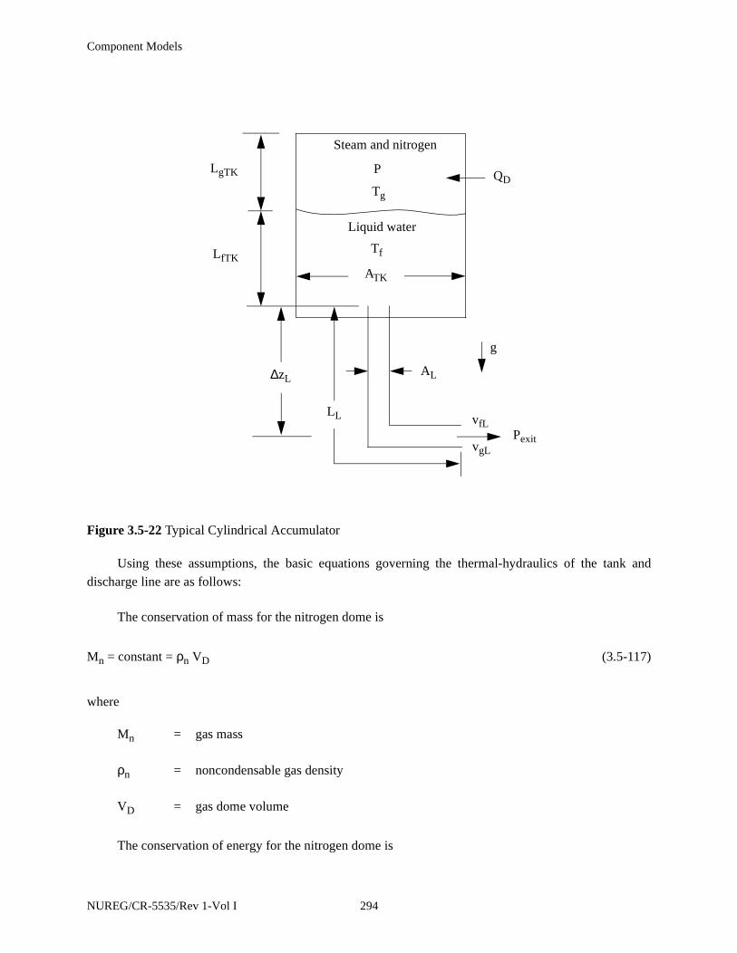
Component Models
Using these assumptions, the basic equations governing the thermal-hydraulics of the tank and
discharge line are as follows:
The conservation of mass for the nitrogen dome is
Mn = constant = ρn VD (3.5-117)
where
Mn = gas mass
ρn = noncondensable gas density
VD = gas dome volume
The conservation of energy for the nitrogen dome is
Figure 3.5-22 Typical Cylindrical Accumulator
Liquid water
Steam and nitrogen
LfTK
LgTK P
Pexit
AL
ATK
vfL
vgL
Tg
Tf
LL
QD
∆zL
g
NUREG/CR-5535/Rev 1-Vol I 294
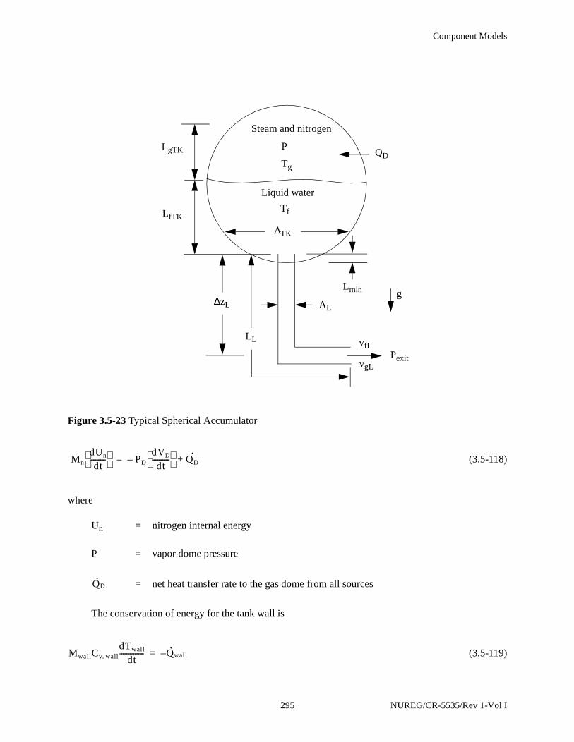
Component Models
(3.5-118)
where
Un = nitrogen internal energy
P = vapor dome pressure
= net heat transfer rate to the gas dome from all sources
The conservation of energy for the tank wall is
(3.5-119)
Figure 3.5-23 Typical Spherical Accumulator
Liquid water
Steam and nitrogen
LfTK
LgTK P
Pexit
AL
ATK
vfL
vgL
Tg
Tf
LL
QD
Lmin
∆zLg
Mn
dUn
dt---------
PD
dVD
dt----------
– QD·
+=
Q· D
MwallCv wall,dTwall
dt-------------- Q· wall–=
295 NUREG/CR-5535/Rev 1-Vol I
Component Models
where
Mwall = metal mass in the tank wall
Cv,wall = metal specific heat
Twall = mean metal temperature
= heat transfer rate to the wall
The conservation of momentum,a for the accumulator tank and surge line is
(3.5−120)
where
A = flow channel cross-sectional area
L = discharge line flow channel length
v = velocity in discharge line
F = frictional loss coefficient
Pexit = pressure at exit of surge line
∆Pz = elevation pressure differential between discharge line entrance and liquid
surface
The equations of state for the noncondensable gas in the dome are,
PVD = MnRnTg (3.5-121)
Un = Mn Cv,n Tg (3.5-122)
Using Equation (3.5-122) in Equation (3.5-118), the nitrogen energy equation, can be rewritten as
a. Equation (3.5-120) is the combined tank and discharge line momentum equation. The wall drag coefficient, F,
is given as , where D = surge line diameter and λwf is the Darcy friction factor.
Q· wall
12---ρfλwf
LD----A v
ρA Ldvdt------
12---v2+
Fv+ A P Pexit–( ) A∆Pz+=
NUREG/CR-5535/Rev 1-Vol I 296
Component Models
(3.5-123)
Differentiating Equation (3.5-121), eliminating the constant term MnRn, and substituting the result
into Equation (3.5-123) yields
(3.5-124)
Equation (3.5-120), (3.5-123), and (3.5-124) comprise the system of three differential equations used
in the accumulator hydrodynamic model. They are used to numerically advance TD, VD, and PD in time.
3.5.7.2 Heat Transfer to the Gas Dome.
In the accumulator, energy transport by convective heat transfer to the gas dome from the walls and
fluid surface is modeled using an empirical Newton cooling law formulation
Qi = hi Ai (Ti - Tg) (3.5-125)
where
i = thermal transport surface
hi = convective heat transfer coefficient (averaged)
Ai = surface area
Ti - Tg = surface to gas dome temperature difference
It should be noted that heat and mass transfer in the accumulator discharge line are neglected.
Two turbulent natural convection heat transfer models are used and combined by superposition.
First, heat transfer with the cylindrical walls of the tank is considered, using a turbulent natural convection
correlation3.5-9 for heat transfer within a vertical cylinder with closed ends for which
(3.5-126)
and
MnCv n,dTg
dt--------- P
dVD
dt----------– Q· D+=
P 1Rn
Cv n,---------+
dVD
dt---------- VD
dPdt------+
Rn
Cv n,---------Q· D=
h1 0.1kD
12--- DTK
--------------- GrPr( )13--- L
δ---
=
297 NUREG/CR-5535/Rev 1-Vol I

Component Models
A1 = πDTKL (3.5-127)
where
h1 = gas dome to cylinder heat transfer coefficient
L = gas dome cylinder length
δ = gas dome characteristic diameter
kn = noncondensable gas thermal conductivity
DTK = tank diameter
Gr = gas dome Grashof number
Pr = gas dome Prandtl number
Second, heat transfer from the disk-shaped ends of the cylinder is considered, where the top disk is
the metal top of the tank and the bottom disk is the liquid-gas interface. For this model, a turbulent natural
convection correlation3.5-9 is used for heat transfer between two horizontal disks separated vertically
where, for each disk,
(3.5-128)
and
(3.5-129)
In the case of a spherical tank, Equation (3.5-126) is used with A1 replaced by the surface area of the
tank in contact with the gas,
A1 = 2πLR (3.5-130)
where L is the height of the gas dome and R is the radius of the sphere. The characteristic diameter of a
spherical gas dome is defined as the ratio of volume to surface area. The correlation given by Equation
(3.5-128) is not used for a spherical tank, hence h2 is set equal to zero.
h2 0.15kn
L----- GrPr( )
13--- L
δ---
=
A2
πDTK2
4-------------=
NUREG/CR-5535/Rev 1-Vol I 298
Component Models
In the correlations given by Equation (3.5-126) and (3.5-128), the product of the Grashof and Prandtl
numbers represents the convective thermal circulation in the gas dome, where the Grashof number
represents the ratio of circulation potential to viscous stress and the Prandtl number represents the ratio of
viscous stress to thermal diffusion. Only the Grashof number is a function of the gas dome dimensions and
temperature difference for which
(3.5-131)
where
g = acceleration due to gravity
βn = noncondensable gas isobaric coefficient of thermal expansion
Ti - Tn = magnitude of the interface, gas dome difference
νn = noncondensable gas kinematic viscosity
δ = characteristic overall diameter of the gas dome
If the Prandtl number is written in terms of the gas dome thermal diffusivity, then
(3.5-132)
where
ρn = noncondensable gas density
αn = noncondensable gas thermal diffusivity
The characteristic diameter is defined in terms of the typical volume-to-surface-area ratio as
(3.5-133)
where Ai is the combined gas dome cylinder, disk top, and bottom surface areas. In the case of a spherical
gas dome, As = A1 + Ai, where A1 is given by Equation (3.5-130) and Ai is the surface area of liquid-gas
interface,
Grgβn Ti Tn– δ3
νn2
----------------------------------=
Prµn
ρnα n-----------=
δ4VD
Ai----------=
299 NUREG/CR-5535/Rev 1-Vol I
Component Models
Ai = πL(2R - L) (3.5-134)
where L is the height of the gas dome and R is the radius of the sphere.
3.5.7.3 Mass Transfer to the Gas Dome.
When the accumulator is in its stagnant initial condition, the gas dome and liquid are in thermal
equilibrium and the gas dome is saturated with water vapor. However, as the accumulator blows down, the
gas dome temperature decreases due to expansion, while the liquid remains essentially isothermal. As a
result, there is simultaneous vaporization at the liquid-gas interface and condensation in the gas dome. This
mechanism transports a large amount of energy to the gas dome as a result of the heat of vaporization of
the water.
At the liquid-gas interface, as vaporization occurs, the relatively warm vapor rapidly diffuses due to
buoyancy into the gas dome. Assuming that the process can be approximated by a quasi-steady
formulation, then for diffusion in a stagnant gas, the mass transfer for the process can be written as
(3.5-135)
where
= rate of vapor diffusion
ζ = diffusion coefficient
Ai = surface area of the liquid-gas interface
= vapor concentration gradient
The concentration can be expressed in terms of partial pressure such that
(3.5-136)
where
C = vapor concentration
Ps = local water vapor partial pressure
M·vap ζAi
dCdx-------–=
M·vap
dCdx-------
CPs
P-----ρs=
NUREG/CR-5535/Rev 1-Vol I 300

Component Models
ρs = water vapor density (saturated vapor at Ps)
Hence, at the dome pressure, the concentration gradient can be written as
(3.5-137)
Combining Equation (3.5-135) and (3.5-137) and integrating gives
(3.5-138)
where the integration is performed by parts.
Both of the differential terms dρs and dPs can be written in terms of temperature differentials if 100%
relative humidity is assumed so that
Ps = Ps (Tg) (3.5-139)
where Ps(Tg) is the saturation pressure at the temperature Tg. Hence, the density differential can be
expanded as
(3.5-140)
where
= κsρs (3.5-141)
= - βsρs (3.5-142)
Combining Equation (3.5-140), (3.5-141), and (3.5-142) and substituting Clapeyron’s equation for
the term gives
dCdx-------
1P---
d Psρs( )dx
------------------=
M·vapLD
ζAi
P-------- Ps ρs ρ Psd
x 0=
x LD=
∫+d
x 0=
x LD=
∫
–=
dρs
∂ρs
∂Ps--------
T
dPs
dT--------
∂ρs
∂T--------
Ps
+ dT=
∂ρs
∂Ps--------
T
∂ρs
∂T--------
Ps
∂ρs
∂Ts--------
301 NUREG/CR-5535/Rev 1-Vol I
Component Models
(3.5-143)
where Clapeyron’s equation is
(3.5-144)
and the term is treated as a constant. Combining Equation (3.5-139), (3.5-143), and (3.5-144), the
diffusion equation can be rewritten as
(3.5-145)
where the dome average terms are evaluated at the dome average temperature, Tg.
Equation (3.5-145) can be made analogous to a convective equation by expressing the mass transfer
coefficient as
(3.5-146)
where h2s is the mass transfer coefficient in a stagnant gas. Then, by applying Reynolds analogy, a
turbulent natural convection mass transfer coefficient can be derived in terms of the heat transfer
coefficient, h2, from Equation (3.5-128) such that
(3.5-147)
where αD is the thermal diffusivity in the gas dome.
Equation (3.5-147) can then be substituted in place of in Equation (3.5-145) to give
dρs ρg κg
hfg
Tgs Vfg
-------------- βg– dT=
dPs hfg
Tgυ fg-------------
dT=
hfg
Tgυ fg-------------
M·vap
ζLD------
Ai
P----- Psρs κ s
hfg
Tgυ fg-------------
βs– ρshfg
Tgυ fg-------------
+
Tf Tg–( )=
h2sζ
LD------=
h2s h2ζ
kD-----
αD
ζ------
1 3⁄
=
ζL---
NUREG/CR-5535/Rev 1-Vol I 302

Component Models
(3.5-148)
which gives the rate at which water vapor is transported into the accumulator gas dome by turbulent
diffusion.
Since the energy transported to the gas dome by the vaporization process must come from the liquid
and since the energy per unit mass required for vaporization is hfg, then the rate of energy transport to the
gas dome by vaporization is
(3.5-149)
where is the rate of vaporization at the liquid gas interface.
In the gas dome, as the accumulator blows down, the gas temperature decreases and condensation of
water vapor occurs. The rate of condensation may be approximated by assuming that the gas dome remains
at 100% humidity and by considering simple humidity relationships. The humidity ratio can be written as
(3.5-150)
where
Ms, Mn = water vapor, gas masses, respectively
Ns, Nn = water vapor, gas molecular weights, respectively
Taking the derivative of Equation (3.5-150) gives
(3.5-151)
From equal Gibb’s free energy, the equilibrium relationship between the vapor and liquid condensate
in the dome is
(3.5-152)
M·vap h2
ζkn-----
α n
ζ-----
13---
Ai
P-----
Psρs κ s
hfg
Tgυ fg-------------
βs– ρshfg
Tgυ fg-------------
+
Tf Tg–( )=
Q· vap M·vaphg Tf( )=
M·vap
wMs
Mn-------
NsPs
NnPD-------------= =
dMs
dt----------
1P--- Mn
Ns
Nn------
dPs
dt-------- Ms
dPdt------–
=
υ s Ps Tg,( )dPs
dTg--------- Ss Ps Tg,( )– υ f P Tg,( ) dP
dTg--------- Sf P Tg,( )–=
303 NUREG/CR-5535/Rev 1-Vol I
Component Models
and substituting the relationship
(3.5-153)
into Equation (3.5-152) and rearranging gives
(3.5-154)
Combining Equation (3.5-151) and (3.5-150) with Equation (3.5-123) and (3.5-124) gives
(3.5-155)
and the rate of condensate formation is given as
(3.5-156)
The energy transported by the condensate to the interface is expressed as
(3.5-157)
Also, since the condensation is taking place in the gas dome, the energy given up by the condensation
process is given up to the gas dome at the rate expressed as
(3.5-158)
Finally, since it is assumed that the condensate is transported to the interface at the condensation rate,
(3.5-159)
the net energy given up to the gas dome by the condensation process can be expressed as
dPdt------
dPdT-------
dTdt-------=
dPs
dt--------
υ f P Tg,( )υs Ps Tg,( )------------------------
dPdt------
hg Ps Tg,( ) hf P Tg,( )–Tgυg Ps Tg,( )
----------------------------------------------------dTg
dt---------–=
dMs
dt----------
1P--- Mn
Ns
Nn------ Ms–
υ f P Tg,( )υs Ps Tg,( )------------------------
1VD------- Q· D
Rn
Cv------ P 1
Rn
Cv------+
dVD
dt----------–=
1P---
Ns
Nn------
hg Ps Tg,( ) hf P Tg,( )–Tgυg Ps Tg,( )
----------------------------------------------------1
Cv n,--------- Q· D P
dVD
dt----------–
+
M·C
dMs
dt----------– M·
vap+=
Q· m· cm· chf
s Tg( )=
Q· M·c
M·chfg Tg( )=
m· c M·c=
NUREG/CR-5535/Rev 1-Vol I 304

Component Models
(3.5-160)
3.5.7.4 Energy Transported to the Gas Dome by Combined Heat and Mass Transfer.
The total energy transported to the gas dome can be rewritten by combining Equation (3.5-125),
(3.5-126), (3.5-128), (3.5-149), and (3.5-160) and summing to give
(3.5-161)
3.5.7.5 Numerical Implementation.
The numerical scheme used for the accumulator model includes special features for coupling the
solution scheme to the main code in such a way that it is time step independent. This scheme is semi-
implicit, and special considerations are employed to preserve the nitrogen energy and mass. Since a
spherical accumulator has a variable cross-sectional area, the momentum equation is generalized to the
case of a variable flow area.
The numerical scheme uses finite-difference techniques to solve the differential equations. The
momentum equation is formulated by integrating Equation (3.5-120) over space and writing the time
variation in difference form as
(3.5-162)
where Pn+1 is the pressure downstream from the accumulator junction. The inertia term is represented by
(3.5-163)
where , , , and are the lengths of the liquid and gas in the discharge line and tank,
respectively, AL is the area of the discharge line, and Af and Ag are the mean flow areas in the tank and
discharge line of the liquid and gas, respectively. In the case of a spherical tank, Ag used in the gas inertia
term is obtained from the relation
Q· c Q· M·c
Q· m· c– m· c hfg Tg( ) hf
s Tg( )–[ ]= =
Q· D h1A1 h2A2+( ) Tw Tg–( ) h2A2 Tf Tg–( ) M·vaphg
s Tf( ) m· c hfg Tg( ) hfs Tg( )–( )+ + +=
ρf LfLLfTK
+( )AL
Af------
Ff∆t ρg Lg L LgTK+( )
AL
Ag------
Fg∆t++ + vfL
n 1+
Pn 1+ PDn 1+–( )∆t– ∆Pz∆t ρ[ fLfL
LfTK+
AL
Af------
+ +=
ρg LgLLgTK
+( )AL
Ag------
]vfL
n CONVF– CONVG–+
ρf LfLLfTK
+( )AL
Af------
ρg LgLLgTK
+( )AL
Ag------
+
LfLLfTK
LgLLgTK
305 NUREG/CR-5535/Rev 1-Vol I
Component Models
(3.5-164)
and Af used in the liquid inertia term is obtained from the relation
(3.5-165)
where and are the gas and liquid volumes, respectively. The volume of gas in the tank is
(3.5-166)
and the available volume of liquid in the tank is
(3.5-167)
where Lmin is the minimum liquid level that is determined by the position of the discharge line which may
protrude into the tank. The inertia terms are computed at each time step and vary explicitly with time; as
the accumulator blows down, the inertia term changes from a liquid-dominant to a vapor-dominant term.
The liquid and gas friction terms, respectively, are formulated as
(3.5-168)
for the liquid, and
(3.5-169)
for the vapor, where friction is neglected in the tank and the line friction factor is assumed to be the
constant turbulent-turbulent Darcy friction factor given as
(3.5-170)
LgTKAg VgTK
=
LfTKAf VfTK
=
VgTKVfTK
VgTKLgTK
( ) π3---LgTK
2 3R LgTK–( )=
VfTKLgTK
( ) 4π3
------R3 VgTK–
π3---Lmin
2 3R Lmin–( )–=
Ff
ρg
2----- λ
LfL
DL------- KL
LfL
LL-------+
vfL
n=
Fg
ρg
2----- λ
LgL
DL-------- KL
LgL
LL--------+
vgL
n=
λ 1.74 2Log102εD-----–
2–
=
NUREG/CR-5535/Rev 1-Vol I 306
Component Models
The loss factor term, KL, is assumed to be distributed over the discharge line length, LL. The term DL
is the surge line hydraulic diameter, and ε is the discharge line wall roughness. The elevation head term,
∆Pz, is formulated as
(3.5-171)
where ∆zTK and ∆zL are the tank and surge line elevation changes, respectively, and g is the gravitational
acceleration. The liquid and vapor momentum flux terms, CONVF and CONVG, respectively are
formulated in linear implicit form as
(3.5-172)
if there is liquid in the tank,
CONVF = 0.0 (3.5-173)
where there is no liquid in the tank,
(3.5-174)
if there is vapor in the discharge line, and, finally
CONVG = 0 (3.5-175)
where there is no vapor in the discharge line. In the case of a spherical tank, the value of ATK used in
CONVF is the flow area at the liquid-gas interface, and the value of ATK used in CONVG is the mean flow
area of the tank. In this formulation, the momentum equation is solved over the pressure gradient from the
centroid of the gas dome to the accumulator junction. However, the momentum of the fluid downstream
from the accumulator junction is not included. Flow begins when the pressure, gravity, and friction forces
result in positive flow out of the accumulator; and flow ceases when these forces result in reverse flow.
Also, since fluxing of the gas through the junction is not allowed,
(3.5-176)
∆Pz
g∆zTK ρfLfTK
12---ρgLgTK
+
LTK-------------------------------------------------------------–
g∆zL ρfLfLρgLgL
+( )LL
-------------------------------------------------–=
CONVF12---ρf 1
AL
Af------
2
– ∆tvfL
n 2vfL
n 1+ vfL
n–( )=
CONVG12---ρg
AL
Af------
2 1
4---
AL
Ag------
2
– ∆tvgL
n 2vgL
n 1+ vgL
n–( )=
vgL
n vfL
n=
307 NUREG/CR-5535/Rev 1-Vol I
Component Models
until the accumulator empties of liquid. The effect of this formulation is that as the accumulator blows
down, the liquid-gas interface moves out of the accumulator tank and surge line. Thus, the centroid of the
gas dome moves towards the centroid of the combined tank and surge line.
The pressure solution is obtained by combining Equation (3.5-118) and (3.5-122) and multiplying by
, which results in
(3.5-177)
where is given by Equation (3.5-161).
Since the liquid is incompressible,
(3.5-178)
and substitution into Equation (3.5-124) and expanding in nonconservative finite difference form gives
(3.5-179)
The energy equation may then be solved directly for the new time gas temperature by combining
Equation (3.5-121), (3.5-124), and (3.5-179) and integrating, which gives
(3.5-180)
The algorithm used to track the liquid level is based on the tank mass balance which is given by
(3.5-181)
In the case of a spherical tank, ATK is given by
(3.5-182)
Rn
Cv n,---------
MnRndTdt-------
RnPCv n,---------
dVD
dt----------–
Rn
Cv n,---------Q· D+=
Q· D
dVD
dt----------
dVf
dt---------– ALvfL
= =
Pn 1Rn
Cvn
-------+ AL∆tvfL
n 1+ VDn Pn 1+ Pn–( )+
Rn
Cv n,---------Q· D
n ∆t=
Tgn 1+ Tg
ne
Rn
Cv n,---------- ln
VDn
VDn 1+
------------- ∆tRn
Cv n,----------
Q· Dn
PnVDn
-------------+
=
ALvfLATK
dLgTK
dt-------------–=
ATK πLgTK2R LgTK
–( )=
NUREG/CR-5535/Rev 1-Vol I 308
Component Models
Given Equation (3.5-181) is solved by explicit numerical integration to obtain ,
(3.5-183)
3.5.8 ECC Mixer
In order to calculate the process of mixing of a jet of cold water injected into a two-phase mixture
and the resulting steam condensation that follows, as in the case of emergency core cooling (ECC)
injection in a PWR, a special component model, called ECCMIX, has been introduced into RELAP5/
MOD3.
3.5.8.1 ECCMIX Component.
An ECC mixing component is a specialized branch that requires three junctions with a certain
numbering order. The physical extent of the ECCMIX component is a length of the cold leg pipe centered
around the position of the ECC injection location. The length of this segment should be about three times
the inside diameter of the cold leg pipe. Junction number one is the ECC connection, junction number two
is the cold leg cross-section through which flow enters this component in normal reactor operation, and
junction number three is the one that leads to the reactor vessel. A schematic vertical cross-section of an
ECCMIX component is shown in Figure 3.5-24. The geometrical description of the ECCMIX component
is very similar to that of the JETMIXER component except for the specification of an angle for the ECC
pipe connection.
The computational model for ECCMIX employs a particular flow regime map for condensation and,
for each flow pattern, uses a different correlation for interfacial heat transfer to calculate hif, as described in
detail in the following subsections. The ECCMIX component calculations are evoked only if there is
subcooled ECC injection and if there is any steam to be condensed in that component. Otherwise, the
ECCMIX component is treated as an ordinary BRANCH in the RELAP5 calculations.
3.5.8.2 Flow Regimes in Condensation.
Prior to the introduction of the ECCMIX component, RELAP5 included three flow regime maps, as
described in the RELAP5/MOD2 manual3.5-10 and in the RELAP5/MOD2 models and correlations
report.3.5-11 None of those, however, would apply specifically to the condensation process in a horizontal
pipe near the emergency core coolant (ECC) injection point. A flow regime map for condensation inside
horizontal tubes is reported by Tandon et al.,3.5-12 and it was considered a more suitable basis for the
interfacial heat transfer calculation in condensation for this geometry. A detailed description of the
resultant ECC mixer volume flow regime map is found in Section 3.3.4 of this volume of the manual.
LgTK
n LgTK
n 1+
LgTK
n 1+ LgTK
n ALvfL
n 1+ ∆tn 1+
πLgTK
n 2R LgTK
n–( )-----------------------------------------–=
309 NUREG/CR-5535/Rev 1-Vol I
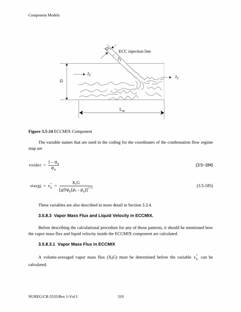
Component Models
The variable names that are used in the coding for the coordinates of the condensation flow regime
map are
(3.5−184)
(3.5-185)
These variables are also described in more detail in Section 3.3.4.
3.5.8.3 Vapor Mass Flux and Liquid Velocity in ECCMIX.
Before describing the calculational procedure for any of those patterns, it should be mentioned how
the vapor mass flux and liquid velocity inside the ECCMIX component are calculated.
3.5.8.3.1 Vapor Mass Flux in ECCMIX
A volume-averaged vapor mass flux (XfG) must be determined before the variable can be
calculated.
Figure 3.5-24 ECCMIX Component
Lm
ECC injection lineD j
J1
J3J2
D
voider1 αg–
αg--------------=
stargj vg* XfG
gDρg ρf ρg–( )[ ] 1 2⁄----------------------------------------------= =
vg*
NUREG/CR-5535/Rev 1-Vol I 310
Component Models
(3.5-186)
where
Wg2 = the total vapor flow rate at junction 2
= αgj2ρgj2vgj2Aj2
Wg3 = the total vapor flow rate at junction 3
= αgj3ρgj3vgj3Aj3
A = cross-sectional area of the ECCMIX component
3.5.8.3.2 Liquid Velocity in ECCMIX
The liquid velocity that is used for determining the Reynolds number inside the ECCMIX component
is calculated on the basis of the smallest of the absolute values of the axial liquid velocity at either end of
the ECC mixer and the additional contribution of the liquid jet from the ECC connection line. The impact
of the incoming ECC liquid jet is a function of the jet velocity vjet and the difference between the pressure
in the hydraulic cell upstream of the injection port and the pressure in the ECCMIX component, ∆Pjet.
(3.5−187)
and
vfres = [∆Ijet + v2fim]1/2 (3.5-188)
where
vfim = min (|vfj2|, |vfj3|)
vfres is the resultant liquid velocity that is used to determine the liquid Reynolds number in heat
transfer and interfacial friction calculations.
3.5.8.4 Interfacial Heat Transfer Rates.
The two-fluid model in RELAP5/MOD3 requires formulation of heat exchange between either phase
and the interface. These are expressed as
XfGWg2 Wg3+
2A-----------------------------=
∆Ijet 2∆Pjet
ρfjet------------=
311 NUREG/CR-5535/Rev 1-Vol I

Component Models
Qik = Hik (Ts - Tk) (3.5-189)
where
k = f or g for liquid and vapor, respectively
Hik = volumetric interfacial heat transfer coefficient for phase k
= hik • Ai
hik = interfacial heat transfer coefficient for phase k
Ai = interfacial area per unit volume
Ts = saturation temperature
Tk = phasic bulk temperature
As implied in Equation (3.5-189), the interface is assumed to be at saturation temperature,
corresponding to the vapor pressure. In condensation of saturated steam, there is almost no temperature
difference between vapor and the interface, while there is a very high rate of heat transfer from the steam to
the interface (through mass transfer). For this reason, the volumetric heat transfer coefficient between
vapor and the interface is set to a high constant value of 107 W/m3⋅K.
The limiting factor is the rate of heat transfer to liquid, Hif. According to Equation (3.5-189), Hif
varies with the heat transfer coefficient, hif, and the interfacial area per unit volume, Ai, both of which
depend on the two-phase flow pattern. The interfacial area, Ai, and the local heat transfer coefficient for
the interface-to-fluid, hif, are calculated with different equations for the six basic flow patterns that are
identified in Table 3.3-1.
3.5.8.4.1 Heat Transfer to Liquid in the Six Basic Flow Patterns
The basic modes of heat transfer to liquid are designed as:
• Hifb1 for wavy flow
• Hifb2 for plug flow
• Hifb3 for slug flow
• Hifb4 for bubbly flow
NUREG/CR-5535/Rev 1-Vol I 312

Component Models
• Hifb5 for annular/annular-mist flow
• Hifb6 for dispersed droplet flow
Heat Transfer in Wavy Flow
Interfacial Area
Wavy flow inside a horizontal tube is regarded as a kind of horizontally stratified flow for the
purpose of interfacial contact and exchanges between vapor and liquid. With this assumption, the
interfacial (contact) area between the liquid and vapor is calculated from the geometrical dimensions of the
ECCMIX component, vapor void fraction, and the diameter of the ECC injection pipe. Figure 3.5-25 and
Figure 3.5-26 show schematic cross-sections of the flow topology inside the ECCMIX component in two
vertical planes.
The volume-average vapor void fraction, αg, is used to determine the width of the liquid surface that
is a function of the half-angle, θ, facing the free surface. RELAP5 uses a particular function, called
HTHETA, to calculate θ for a given volume fraction that is bound by θ. If the liquid level is above the pipe
center (αg < αf), then HTHETA is called with αg as an argument and θ is calculated. However, if αg > αf,
then αf is used as an argument for calculating θ. For this reason, care is taken to calculate the length of the
liquid jet, Ljet, differently for these cases, as the cylindrical surface of the liquid jet is also a part of the
condensation surface. The jet surface area is given by
Ajet = π djet • Ljet (3.5-190)
Figure 3.5-25 Schematic Cross-Section of Stratified Flow Along the ECCMIX Component, Showing the Length of Interface (Lm) and the Jet Length (Ljet)
Ljet
Lm
φ (
313 NUREG/CR-5535/Rev 1-Vol I
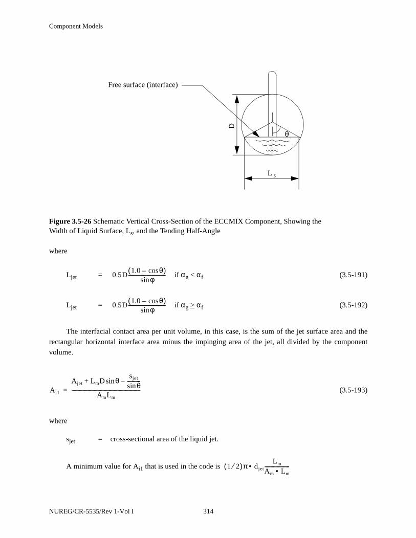
Component Models
where
Ljet = if αg < αf (3.5-191)
Ljet = if αg > αf (3.5-192)
The interfacial contact area per unit volume, in this case, is the sum of the jet surface area and the
rectangular horizontal interface area minus the impinging area of the jet, all divided by the component
volume.
(3.5-193)
where
sjet = cross-sectional area of the liquid jet.
A minimum value for Ai1 that is used in the code is
Figure 3.5-26 Schematic Vertical Cross-Section of the ECCMIX Component, Showing the Width of Liquid Surface, Ls, and the Tending Half-Angle
θ
L s
D
Free surface (interface)
0.5D1.0 θcos–( )
φsin------------------------------
0.5D1.0 θcos–( )
φsin------------------------------
Ai1
Ajet LmD θsinsjet
θsin-----------–+
AmLm-------------------------------------------------------=
1 2⁄( )π djet•Lm
Am Lm•--------------------
NUREG/CR-5535/Rev 1-Vol I 314
Component Models
Heat Transfer Coefficient
The heat transfer coefficient for wavy flow is calculated according to an experimentally established
correlation by Lim, Bankoff, Tankin, and Yuen,3.5-13 based on their data from condensation in cocurrent
flow of vapor and liquid in a horizontally stratified flow situation. The correlation that is taken from
Reference 3.5-13 is the one that is recommended for the case of rough liquid surface, namely
(3.5-194)
where
Nu = Nusselt number
Re = Reynolds number
Pr = Prandtl number (see nomenclature)
Using this correlation for Nusselt number, the overall heat transfer coefficient from the interface to
liquid, per unit volume, in wavy flow is expressed as
(3.5-195)
Heat Transfer in Plug Flow
Interfacial Area
According to the flow regime map (Figure 3.3-4), this flow pattern exists for vapor void fractions
between 0.25 and 0.666. It is assumed that the interfacial area changes from completely stratified at voider
= 0.5 (αg = 0.666) to a complete circular cross-section of the ECCMIX component at voider = 3.0 (for α =
0.25). Hence, the interface area is interpolated between these limits, using the following parameter
tv1 = 0.4 (voider - 0.5) for 0.5 < voider < 3.0 (3.5-196)
The interfacial area for the stratified flow condition is calculated according to Equation (3.5-193),
and the interpolated area for wavy flow is
(3.5-197)
Nu 0.0344 Re( )g0.58 Re( )f
0.42 Pr( )f0.33=
Hifb1 Ai1Nukfm
D-------
=
A12 1.0 tv1–( )Ai1 tv11
Lm------
+=
315 NUREG/CR-5535/Rev 1-Vol I

Component Models
Heat Transfer Coefficient
Since plug flow is considered an extension of the wavy flow pattern with interrupting liquid plugs,
the same heat transfer coefficient that was used for wavy flow, Equation (3.5-194), has been used for plug
flow. Hence, the overall heat transfer coefficient from interface to liquid, per unit volume, in plug flow is
(3.5-198)
in which Nu is given by Equation (3.5-194).
Heat Transfer in Slug Flow
Interfacial Area
Slug flow is assumed to always include some contribution of the bubbly flow pattern; hence, there is
a gradual changeover from slug flow to a pure bubbly flow. The degree of this transition depends on vapor
void fraction. This approach is used for all volumes in RELAP5/MOD3 (see Volume IV). There is only a
slight modification in the application of this approach to the ECCMIX component, that is, the lower limit
of vapor void fraction is set at αb = 0.20 and the upper end void fraction is set at αc = 0.666. These changes
had to be imposed according to the limits specified for slug flow in the modified flow regime map for
condensation, as shown in Figure 3.3-4.
The interfacial area of slug bubbles (these are called Taylor bubbles in Reference 3.5-11) per unit
volume is calculated as
(3.5-199)
where
αs = (3.5-200)
αbb = (3.5-201)
The numerical value of αbb varies from 0.2 (αb) when αg = αb to about 0.0002277 when αg = αc. As
a result, Ai3s varies from 0.0 at αg = 0.2 to about for αg = αc.
Hifb2 Ai2Nukfm
D-------
=
Ai3s 4.5α s
D-----=
1 αg–( ) αbb–1 αbb–
---------------------------------
αbexp6.778
α c αb–----------------- αg αb–( )–
4.51.0 αg–
Dc-------------------
NUREG/CR-5535/Rev 1-Vol I 316
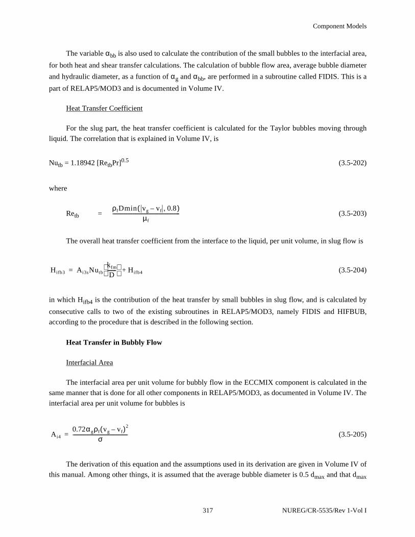
Component Models
The variable αbb is also used to calculate the contribution of the small bubbles to the interfacial area,
for both heat and shear transfer calculations. The calculation of bubble flow area, average bubble diameter
and hydraulic diameter, as a function of αg and αbb, are performed in a subroutine called FIDIS. This is a
part of RELAP5/MOD3 and is documented in Volume IV.
Heat Transfer Coefficient
For the slug part, the heat transfer coefficient is calculated for the Taylor bubbles moving through
liquid. The correlation that is explained in Volume IV, is
Nutb = 1.18942 [RetbPr]0.5 (3.5-202)
where
Retb = (3.5-203)
The overall heat transfer coefficient from the interface to the liquid, per unit volume, in slug flow is
(3.5-204)
in which Hifb4 is the contribution of the heat transfer by small bubbles in slug flow, and is calculated by
consecutive calls to two of the existing subroutines in RELAP5/MOD3, namely FIDIS and HIFBUB,
according to the procedure that is described in the following section.
Heat Transfer in Bubbly Flow
Interfacial Area
The interfacial area per unit volume for bubbly flow in the ECCMIX component is calculated in the
same manner that is done for all other components in RELAP5/MOD3, as documented in Volume IV. The
interfacial area per unit volume for bubbles is
(3.5-205)
The derivation of this equation and the assumptions used in its derivation are given in Volume IV of
this manual. Among other things, it is assumed that the average bubble diameter is 0.5 dmax and that dmax
ρfDmin vg vf– 0.8,( )µf
------------------------------------------------------
Hifb3 Ai3sNutb
kfm
D-------
Hifb4+=
Ai4
0.72αgρf vg vf–( )2
σ--------------------------------------------=
317 NUREG/CR-5535/Rev 1-Vol I

Component Models
is determined by using a critical Weber number of Wec = 10. Computation of Ai4 is done by using the
FIDIS subroutine in RELAP5.
Heat Transfer Coefficient
For the bubbly flow regime, the heat transfer coefficient between the interface and liquid is
calculated with a model based on the modified Unal bubble collapse model3.5-14,3.5-15 and the Lahey
model.3.5-16 This is the same model that is used in non-ECCMIX volumes.
The heat transfer coefficient between the interface and liquid, per unit volume, in bubbly flow that is
calculated in the HIFBUB subroutine is according to the following equation:
(3.5-206)
where
F5 = 0.075 for αbub > 0.25 (3.5-207)
F5 = 1.8φC exp(-45αbub) + 0.075 for αbub < 0.25 (3.5-208)
C = 65.0 - 5.69 x 10⁻⁵ (P - 1.0 x 10⁵) for P < 1.1272 x 10⁶ (3.5-209)
C = 2.5 x 10⁹ P-1.418 for P > 1.1272 x 10⁶ (3.5-210)
φ = 1.0 for |vf| < 0.61 m/s (3.5-211)
φ = [1.639344 |vf|]0.47 for |vf| > 0.61 m/s (3.5-212)
αbub = max(αg, 10-5) (3.5-213)
Heat Transfer in Annular/Annular-Mist Flow
Heat transfer between interface and liquid in the annular and annular-mist flow regimes is calculated
according to the procedures that are used in TRAC-BF1.3.5-17,3.5-18 According to this model, the interfacial
exchanges of heat and momentum at the interface have two components, one at the interface between the
vapor core and the liquid film on the walls and another one at the interface between the vapor and the
entrained liquid droplets. The contribution of the entrained droplets is minimal at the start of the annular
flow, but the entrained liquid fraction increases with increasing vapor velocity and it becomes 100% at the
end of the annular flow, that is the start of dispersed droplet (mist) flow. Variations of the entrainment
Hifb4
F5αghfgρfρg
ρf ρg–-----------------------------=
NUREG/CR-5535/Rev 1-Vol I 318
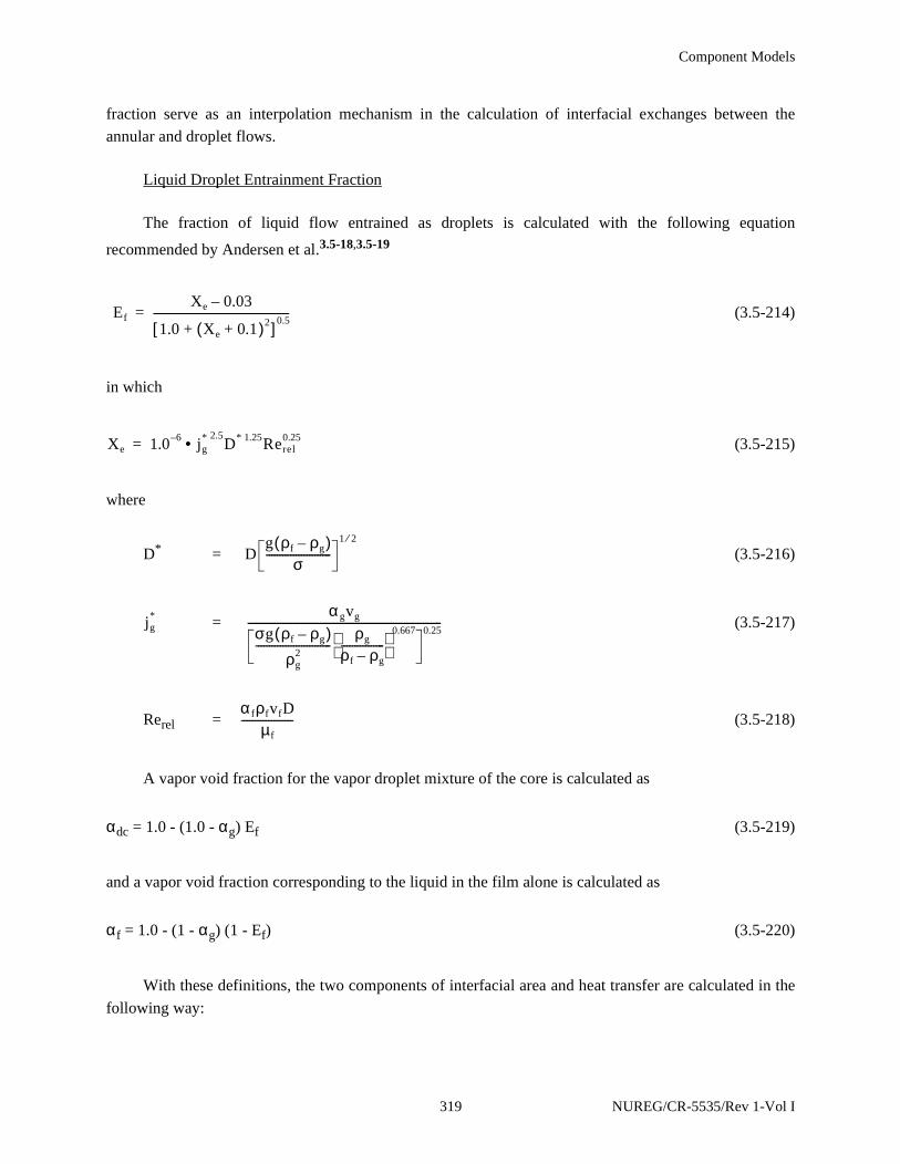
Component Models
fraction serve as an interpolation mechanism in the calculation of interfacial exchanges between the
annular and droplet flows.
Liquid Droplet Entrainment Fraction
The fraction of liquid flow entrained as droplets is calculated with the following equation
recommended by Andersen et al.3.5-18,3.5-19
(3.5-214)
in which
(3.5-215)
where
D* = (3.5-216)
= (3.5-217)
Rerel = (3.5-218)
A vapor void fraction for the vapor droplet mixture of the core is calculated as
αdc = 1.0 - (1.0 - αg) Ef (3.5-219)
and a vapor void fraction corresponding to the liquid in the film alone is calculated as
αf = 1.0 - (1 - αg) (1 - Ef) (3.5-220)
With these definitions, the two components of interfacial area and heat transfer are calculated in the
following way:
Ef
Xe 0.03–
1.0 Xe 0.1+( )2+[ ] 0.5--------------------------------------------------=
Xe 1.0 6– jg* • 2.5
D* 1.25Rerel0.25=
Dg ρf ρg–( )
σ------------------------
1 2⁄
jg* α gvg
σg ρf ρg–( )ρg
2----------------------------
ρg
ρf ρg–----------------
0.667 0.25
------------------------------------------------------------------------
α fρfvfDµf
-------------------
319 NUREG/CR-5535/Rev 1-Vol I

Component Models
Film Interfacial Area
The average film thickness is
δf = 0.5 D(1.0 - αf)0.5 (3.5-221)
A minimum film thickness is calculated as3.5-18,3.5-19
(3.5-222)
The average film thickness is selected as
δfa = max (δf, δfmin) (3.5-223)
A void fraction corresponding to δfmin is calculated as
(3.5-224)
Since the inside diameter of the liquid film is related to the inside diameter of the channel, Dc,
through αf by the relationship Di = Dc(αf)1/2, the interfacial area per unit volume for the liquid film is then
(3.5-225)
If αmin < αg, then
(3.5-226)
Droplet Interfacial Area
According to Reference 3.5-19, an average droplet diameter is calculated based on the total mass
flux, jmt
δfmin
18µf2σ
g2ρf3
---------------
0.2
=
αmin 1.02δfmin
D--------------–
2
=
Ai5f 4.0α f( )1 2⁄
D----------------=
Ai5f 4α f( )1 2⁄
D----------------
1.0 α f–1.0 αmin–------------------------=
NUREG/CR-5535/Rev 1-Vol I 320
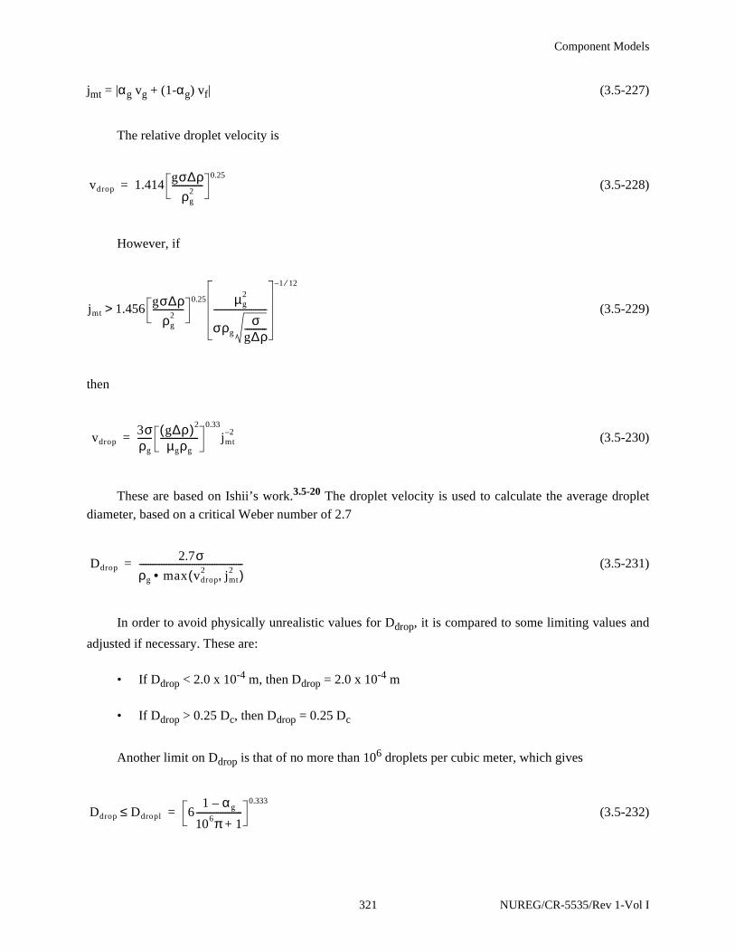
Component Models
jmt = |αg vg + (1-αg) vf| (3.5-227)
The relative droplet velocity is
(3.5-228)
However, if
(3.5-229)
then
(3.5-230)
These are based on Ishii’s work.3.5-20 The droplet velocity is used to calculate the average droplet
diameter, based on a critical Weber number of 2.7
(3.5-231)
In order to avoid physically unrealistic values for Ddrop, it is compared to some limiting values and
adjusted if necessary. These are:
• If Ddrop < 2.0 x 10⁻⁴ m, then Ddrop = 2.0 x 10⁻⁴ m
• If Ddrop > 0.25 Dc, then Ddrop = 0.25 Dc
Another limit on Ddrop is that of no more than 106 droplets per cubic meter, which gives
(3.5-232)
vdrop 1.414gσ∆ρ
ρg2
--------------0.25
=
jmt 1.456gσ∆ρ
ρg2
--------------0.25 µg
2
σρgσ
g∆ρ----------
------------------------
1 12⁄–
>
vdrop3σρg------
g∆ρ( )2
µgρg-----------------
0.33
jmt2–=
Ddrop2.7σ
ρg max vdrop2 jmt
2,( )•-----------------------------------------------=
Ddrop Ddropl≤ 61 αg–
106π 1+---------------------
0.333
=
321 NUREG/CR-5535/Rev 1-Vol I
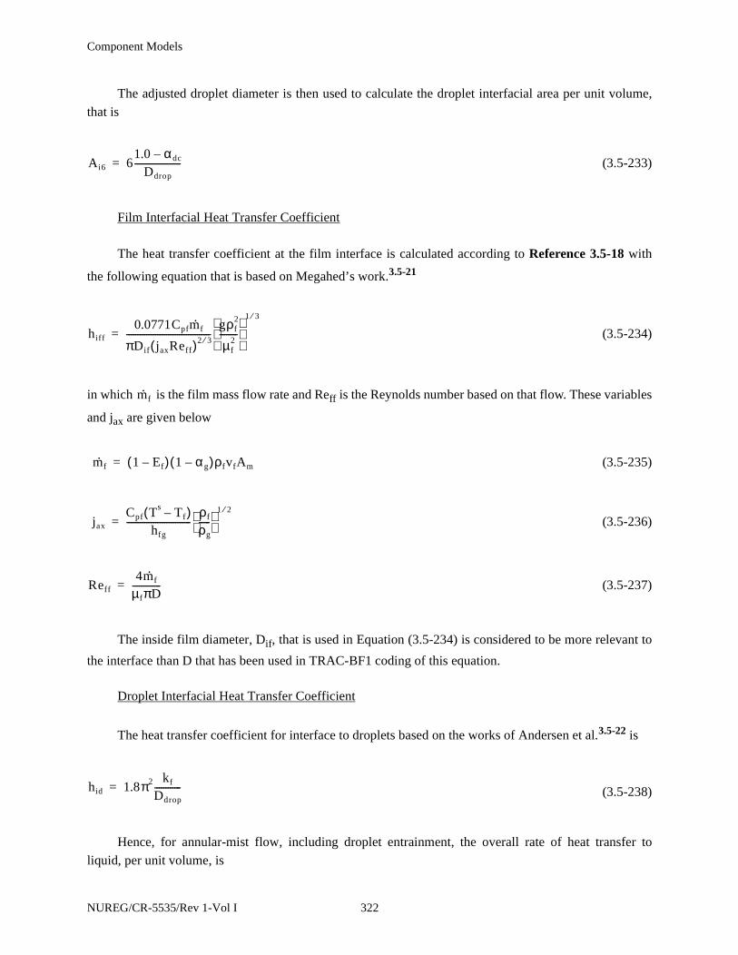
Component Models
The adjusted droplet diameter is then used to calculate the droplet interfacial area per unit volume,
that is
(3.5-233)
Film Interfacial Heat Transfer Coefficient
The heat transfer coefficient at the film interface is calculated according to Reference 3.5-18 with
the following equation that is based on Megahed’s work.3.5-21
(3.5-234)
in which is the film mass flow rate and Reff is the Reynolds number based on that flow. These variables
and jax are given below
(3.5-235)
(3.5-236)
(3.5-237)
The inside film diameter, Dif, that is used in Equation (3.5-234) is considered to be more relevant to
the interface than D that has been used in TRAC-BF1 coding of this equation.
Droplet Interfacial Heat Transfer Coefficient
The heat transfer coefficient for interface to droplets based on the works of Andersen et al.3.5-22 is
(3.5-238)
Hence, for annular-mist flow, including droplet entrainment, the overall rate of heat transfer to
liquid, per unit volume, is
Ai6 61.0 αdc–
Ddrop---------------------=
hiff
0.0771Cpfm· f
πDif jaxReff( )2 3⁄--------------------------------------gρf
2
µf2
--------
1 3⁄
=
m· f
m· f 1 Ef–( ) 1 αg–( )ρfvfAm=
jax
Cpf Ts Tf–( )hfg
-----------------------------ρf
ρg-----
1 2⁄
=
Reff
4m· f
µfπD-------------=
hid 1.8π2 kf
Ddrop------------=
NUREG/CR-5535/Rev 1-Vol I 322

Component Models
Hifb5 = Ai5fhiff + Ai6hid (3.5-239)
Heat Transfer in Dispersed Droplet Flow
The interfacial area per unit volume and the heat transfer coefficient for droplets were described
above. The overall heat transfer rate to liquid in this flow regime is
Hifb6 = Ai6hid (3.5-240)
where Ai6 and hid are given by Equation (3.5-233) and (3.5-238), respectively.
3.5.8.4.2 Heat Transfer to Liquid in Transition Zones
As shown in Table 3.3-1, there are five transition zones in the modified condensation flow regime
map. The numerical values of the heat transfer rates, Hif, in the adjacent zones of the basic mode may vary
considerably, and a linear interpolation over the boundary zones would not be adequate to produce a
smooth transition. For this reason, an exponential interpolation is employed, as detailed in the following.
For transition between wavy and annular-mist flows,
(3.5-241)
where
van =
For transition between wavy and slug flows,
(3.5-242)
where
psw = (3.5-243)
For transition between wavy, plug, and slug flows (double interpolation), first an interpolation is
made in terms of and then another one in terms of .
Hift1 Hifb51 van–( )Hifb1
van=
9 8 vg* for 1 vg
* 1.125≤ ≤–
Hift2 Hifb3psw Hifb1
1 psw–( )=
81 α–
α------------ 4 for 0.5
1 α–α
------------ 0.625≤ ≤–
vg* 1 α–
α------------
323 NUREG/CR-5535/Rev 1-Vol I

Component Models
(3.5-244)
where
Hiftsp = (3.5-245)
p1 = (3.5-246)
p2 = (3.5-247)
For transition between plug and slug flows
(3.5-248)
where
pp = (3.5-249)
Finally, for transition between bubbly and plug flows
(3.5-250)
where
pb = - 3.0 for 3.0 (3.5-251)
Computation of the interfacial heat transfer according to these equations is done in the ECCMXV
subroutine, that is called within subroutine PHANTV, whenever the ECCMIX component is encountered
and specific logical tests indicate that there is some vapor in this component and a flow of subcooled liquid
is entering through the ECC injection line. Otherwise, the ECCMIX component is treated just as a regular
BRANCH component in the RELAP5/MOD3 calculations.
3.5.8.5 Effect of Noncondensable Gases.
It is known that the presence of noncondensable gases, such as air or pure nitrogen, reduces the rate
of condensation. An experimental study of the effect of noncondensable gases at different partial pressures
on the rate of condensation heat transfer is reported by DeVuono and Christensen.3.5-23 According to their
Hift3 Hiftspp2 Hifb1
1 p2–( )=
Hifb21 p1–( )Hifb3
p1
400vg* 4. for 0.01 vg
* 0.0125≤ ≤–
81 α–
α------------ 4. for 0.5
1 α–α
------------ 0.625≤ ≤–
Hift4 Hifb21 pp–( )Hifb3
1 pp–( )=
400vg* 4. for 0.01 vg
* 0.0125≤ ≤–
Hift5 Hifb4pb Hifb2
1 pb–( )=
1 α–α
------------1 α–
α------------ 4.0≤ ≤
NUREG/CR-5535/Rev 1-Vol I 324

Component Models
findings, the degradation in the condensation heat transfer with concentration of air can be correlated with
the following:
fr = (1. - y)4.31 for 0 < y < 0.14 (3.5-252)
where
fr = reduction factor in condensation heat transfer
y = air concentration (air volume at prevailing pressure and time divided by totalvolume)
The reduction factor, fr, of Equation (3.5-252) is applied to Hif as calculated in the ECCMXV
subroutine. It should be noted that the actual plots of measured data reported in Reference 3.5-23 indicate
a much stronger sensitivity to air concentration as compared to what can be calculated with their
correlation.
3.5.8.6 Interfacial Friction.
Calculation of the interfacial friction for different flow patterns in the ECCMIX component is done
with the same correlations that are used for similar flow patterns in all other horizontal components in
RELAP5/MOD3. The only remarks to be made on the interfacial friction calculations in the ECCMIX
components are the following:
• Transition between different flow patterns is according to the modified condensationflow regime map.
• Linear interpolation is used between the friction values of the basic pattern around eachinterpolation zone, employing the same interpolation variables that were used forinterfacial heat transfer in those boundary zones.
• For plug flow, it is assumed that the two phases are locked into each other; hence, theinterfacial friction factor is set to 1.
Computation of the interfacial friction factors is performed in a separate subroutine called ECCMXJ,
whenever the ECCMIX component is encountered and specific logical tests indicate that there is some
vapor in the ECCMIX component and that a flow of subcooled liquid is entering through the ECC
injection line. Otherwise, the ECCMIX component is treated just as a regular BRANCH in the RELAP5/
MOD3 calculations.
325 NUREG/CR-5535/Rev 1-Vol I
Component Models
3.5.8.7 Wall Friction.
The two-fluid model of RELAP5/MOD3 requires that each phase should have its own fraction of the
wall friction for momentum balance. The distribution of the total wall friction between vapor and liquid
varies with flow regimes. Calculations of the fractions of wall friction for each phase in different flow
regimes are done according to the same procedures that are used in other components. However, transition
between different flow regimes is determined in the same way that is used for the interfacial heat and
momentum transfer calculations. The only differences that are introduced for wall friction in the ECCMIX
component are the following:
• In bubbly flow, 100% of the wall friction is assigned to the liquid phase and nothing tothe vapor phase.
• In droplet flow, 100% of the wall friction is assigned to the vapor phase and nothing tothe liquid phase.
• Linear interpolation is used for wall friction over the transition zones, employing thesame interpolation variables that were defined for the interfacial heat transfer.
Computations of wall friction fractions for vapor and liquid are performed in parallel with the Hif
calculations in the ECCMXV subroutine.
3.5.9 Annulus
For an annulus component in the annular-mist regime for both the junction and volume flow regimes,
the code assumes that all the liquid is in the film and that there are no drops. Thus, αff = αf and αfd = 0.
This was based on work by Schneider3.5-24 on RELAP5/MOD3 calculations for UPTF Test 6, who showed
that this was necessary in order to get downcomer penetration following a cold leg break. In addition, the
Bharathan3.5-25 correlation used in RELAP5/MOD2 was replaced by a standard laminar correlation and
the modified Wallis3.5-26 correlation in the turbulent region for the interfacial drag when in the annular-
mist flow regime (for either an annulus or any other component). Schneider found this was also necessary
in order to get downcomer penetration in UPTF Test 6. This interphase drag approach for an annulus
component was also used in RELAP5/MOD1.
3.5.10 References
3.5-1. Y. K. Cheung, V. Parameswaran, and J. .C. Shaug. BWR Refill-Reflood Program, Task 4.7-ModelDevelopment, TRAC-BWR Component Models. NUREG/CR-2574, EPRI NP-2376, GEAP-22052. April 1983.
3.5-2. R. H. Moen, et al. “Advances in Boiling Water Reactor Steam Separator Systems.” ASME-60-WA/NE-5. November 1969.
NUREG/CR-5535/Rev 1-Vol I 326
Component Models
3.5-3. E. L. Burley. “Performance of Internal Steam Separator System in Boiling Water Reactors.”ASME-69-WA/NE-24. November 1969.
3.5-4. S. Wolf and R. H. Moen. “Advances in Steam-Water Separators for Boiling Water Reactors.”ASME-73-WA/PWR-4. November 1973.
3.5-5. V. H. Ransom et al. RELAP5/MOD1 Code Manual. NUREG/CR-4312, EGG-2070. IdahoNational Engineering Laboratory. March 1982.
3.5-6. EG&G Idaho, Inc. RELAP4/MOD6: A Computer Program for Transient Thermal-HydraulicAnalysis of Nuclear Reactors and Related Systems, Users Manual. CDAP-TR-003. IdahoNational Engineering Laboratory. May 1978.
3.5-7. J. K. Salisbury. Steam Turbines and Their Cycles. New York: Kreiger. 1950.
3.5-8. J. K. Vennard and R. L. Street. Elementary Fluid Mechanics. 6th Edition. New York: John Wileyand Sons. 1982.
3.5-9. J. P. Holman. Heat Transfer. 4th Edition. New York: McGraw-Hill Book Company, Inc. 1976.pp. 244-245. 280.
3.5-10. V. H. Ransom et al. RELAP5/MOD2 Code Manual. NUREG/CR-4312, EGG-2396. IdahoNational Engineering Laboratory. August 1985 and December 1985. revised March 1987.
3.5-11. R. A. Dimenna et al. RELAP5/MOD2 Models and Correlations. NUREG/CR-5194, EGG-2531.Idaho National Engineering Laboratory. August 1988.
3.5-12. T. N. Tandon, H. K. Varma, and C. P. Gupta. “A New Flow Regime Map for Condensation InsideHorizontal Tubes.” Journal of Heat Transfer. 104. November 1982. pp. 763-768.
3.5-13. I. S. Lim, S. G. Bankoff, R. S. Tankin, and M. C. Yeun. Co-current Steam/Water Flow in aHorizontal Channel. NUREG/CR-2289. August 1981.
3.5-14. H. C. Unal. “Maximum Bubble Diameter, Maximum Bubble-Growth Time and Bubble-Growth
Rate During the Subcooled Nucleate Flow Boiling of Water up to 17.7 MN/m2.” InternationalJournal of Heat Mass Transfer. 19. 1976. pp. 643-649.
3.5-15. R. A. Riemke. “Modification to Unal’s Subcooled Flow Boiling Bubble Model.” NuclearTechnology. 102. 1993. pp. 416-417.
3.5-16. R. T. Lahey. “A Mechanistic Subcooled Boiling Model.” Proceedings from Sixth InternationalHeat Transfer Conference, Toronto, Canada, 1978. Volume 1. pp. 293-297.
3.5-17. W. L. Weaver et al. TRAC-BF1 Manual: Extensions to TRAC-BD1/MOD1. NUREG/CR-4391,EGG-2417. Idaho National Engineering Laboratory. August 1986.
327 NUREG/CR-5535/Rev 1-Vol I

Component Models
3.5-18. S. Z. Rouhani et al. TRAC-BF1 Models and Correlations. NUREG/CR-4391, EGG-2680. IdahoNational Engineering Laboratory. August 1992.
3.5-19. J. M. G. Andersen, K. H. Chu, and J. C. Shaug. BWR Refill-Reflood Program, Task 4.7--ModelDevelopment, Basic Models for the BWR Version of TRAC. NUREG/CR-2573, EPRI NP-2375,GEAP-22051. September 1983.
3.5-20. M. Ishii. One-Dimensional Drift-Flux Model and Constitutive Equations for Relative MotionBetween Phases in Various Two-Phase Flow Regimes. ANL-77-47. Argonne NationalLaboratory. October 1977.
3.5-21. M. M. Megahed. Interfacial Heat Transfer Countercurrent Flows of Steam and Water. EGG-RTH-2495. Idaho National Engineering Laboratory. January 1987.
3.5-22. J. G. M. Andersen and H. Abel-Larsen. CORECOOL-Model Description of the Program. RISO-M-21380. November 1980.
3.5-23. A. C. DeVuono and R. N. Christensen. “Experimental Investigation of the Pressure Effect onFilm Condensation of Steam-Air Mixture at Pressure Above Atmospheric.” Fundamentals ofPhase Change: Boiling and Condensation. ASME-HTD Vol. 38. 1984. pp. 73-80.
3.5-24. K. Schneider. “Siemens Contributions to RCP Modeling and Evaluation of UPTF Test 6.” ICAPMeeting, Bethesda, MD. October 18-20, 1989.
3.5-25. D. Bharanthan, G. B. Wallis, and H. T. Richter. Air-Water Counter-Current Annular Flow. EPRINP-1165. 1979.
3.5-26. G. B. Wallis. One-Dimensional Two-Phase Flow. New York: McGraw-Hill Book Company.1969.
NUREG/CR-5535/Rev 1-Vol I 328

HEAT STRUCTURE MODELS
4 HEAT STRUCTURE MODELS
4.1 Heat Conduction Numerical Techniques
Heat structures provided in RELAP5 permit calculation of the heat transferred across solid
boundaries of hydrodynamic volumes. Modeling capabilities of heat structures are general and include fuel
pins or plates with nuclear or electrical heating, heat transfer across steam generator tubes, and heat
transfer from pipe and vessel walls. Heat structures are assumed to be represented by one-dimensional heat
conduction in rectangular, cylindrical, or spherical geometry. Surface multipliers are used to convert the
unit surface of the one-dimensional calculation to the actual surface of the heat structure. Temperature-
dependent thermal conductivities and volumetric heat capacities are provided in tabular or functional form
either from built-in or user-supplied data.
Finite differences are used to advance the heat conduction solutions. Each mesh interval may contain
a different mesh spacing, a different material, or both. The spatial dependence of the internal heat source
may vary over each mesh interval. The time-dependence of the heat source can be obtained from reactor
kinetics, one of several tables of power versus time, or a control system variable. Boundary conditions
include symmetry or insulated conditions, a correlation package, tables of surface temperature versus time,
heat transfer rate versus time, and heat transfer coefficient versus time or surface temperature. The heat
transfer correlation package can be used for heat structure surfaces connected to hydrodynamic volumes,
and contains correlations for convective, nucleate boiling, transition boiling, and film boiling heat transfer
from the wall to water and reverse transfer from water to wall including condensation.
The following describes the numerical techniques for heat conduction. The integral form of the heat
conduction equation is
(4.1-1)
where
k = the thermal conductivity
s = the surface
S = the internal heat source
t = time
T = temperature
V = volume
ρ T x,( )∂T∂t------ x t,( )dV∫
V
∫∫ k T x,( )∇ T x t,( ) ds S x t,( )dV∫V
∫∫+•S
∫∫=
329 NUREG/CR-5535/Rev 1-Vol I
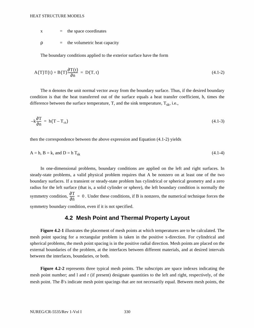
HEAT STRUCTURE MODELS
x = the space coordinates
ρ = the volumetric heat capacity
The boundary conditions applied to the exterior surface have the form
(4.1-2)
The n denotes the unit normal vector away from the boundary surface. Thus, if the desired boundary
condition is that the heat transferred out of the surface equals a heat transfer coefficient, h, times the
difference between the surface temperature, T, and the sink temperature, Tsk, i.e.,
(4.1-3)
then the correspondence between the above expression and Equation (4.1-2) yields
A = h, B = k, and D = h Tsk (4.1-4)
In one-dimensional problems, boundary conditions are applied on the left and right surfaces. In
steady-state problems, a valid physical problem requires that A be nonzero on at least one of the two
boundary surfaces. If a transient or steady-state problem has cylindrical or spherical geometry and a zero
radius for the left surface (that is, a solid cylinder or sphere), the left boundary condition is normally the
symmetry condition, . Under these conditions, if B is nonzero, the numerical technique forces the
symmetry boundary condition, even if it is not specified.
4.2 Mesh Point and Thermal Property Layout
Figure 4.2-1 illustrates the placement of mesh points at which temperatures are to be calculated. The
mesh point spacing for a rectangular problem is taken in the positive x-direction. For cylindrical and
spherical problems, the mesh point spacing is in the positive radial direction. Mesh points are placed on the
external boundaries of the problem, at the interfaces between different materials, and at desired intervals
between the interfaces, boundaries, or both.
Figure 4.2-2 represents three typical mesh points. The subscripts are space indexes indicating the
mesh point number; and l and r (if present) designate quantities to the left and right, respectively, of the
mesh point. The δ’s indicate mesh point spacings that are not necessarily equal. Between mesh points, the
A T( )T t( ) B T( )∂T t( )∂n
-------------+ D T t,( )=
k∂T∂n------– h T Tsk–( )=
∂T∂n------ 0=
NUREG/CR-5535/Rev 1-Vol I 330

HEAT STRUCTURE MODELS
thermal properties, k and ρ, and the source term, S, are assumed spatially constant; but klm is not
necessarily equal to krm and similarly for ρ and S.
To obtain the spatial-difference approximation for the m-th interior mesh point, Equation (4.1-1) is
applied to the volume and surfaces indicated by the dashed line shown in Figure 4.2-2. For the spatial
difference approximation at the boundaries, Equation (4.1-1) is applied to the volumes and interior
surfaces indicated by the dashed lines shown in Figure 4.2-3 and Equation (4.1-2) is used to define the
gradient along the exterior surfaces. If the coefficient of the gradient in the boundary equation is zero, the
surface temperature is given directly from Equation (4.1-2). Since the code is one-dimensional, the
dimensions of the volume for other than the x or r coordinate are set to one. For rectangular geometry, the
volume is a rectangular solid. For cylindrical geometry, the volume is a cylindrical annulus; and for
spherical geometry, the volume is a spherical shell.
The spatial finite-difference approximations use exact expressions for the space and volume factors
and simple differences for the gradient terms. To condense the expressions defining the numerical
Figure 4.2-1 Mesh Point Layout
Figure 4.2-2 Typical Mesh Points
Compositioninterfaces
Boundary
Mesh points
Mesh pointnumbering
1 2 3 4 etc.
Boundary
m-1
δlm mδrm
δlm
Slm
ρlm
klm krmρrmSrm
m+1
2δrm2
331 NUREG/CR-5535/Rev 1-Vol I
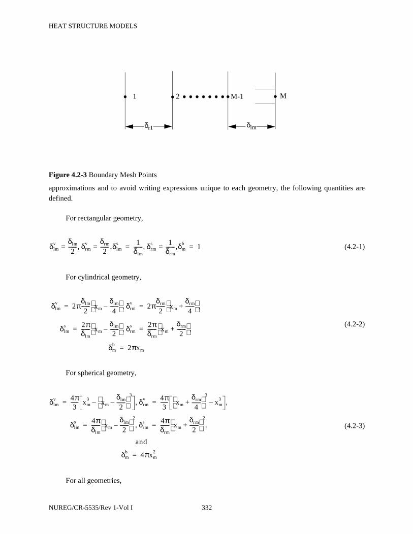
HEAT STRUCTURE MODELS
approximations and to avoid writing expressions unique to each geometry, the following quantities are
defined.
For rectangular geometry,
(4.2-1)
For cylindrical geometry,
(4.2-2)
For spherical geometry,
(4.2-3)
For all geometries,
Figure 4.2-3 Boundary Mesh Points
δr1 δlm
M-12 M1
δlmv δlm
2------- δrm
v δrm
2-------,=,= δlm
s 1δlm------- δrm
s 1δrm-------,δm
b=, 1= =
δlmv 2π
δlm
2------- xm
δlm
4-------–
δrmv, 2π
δrm
2------- xm
δrm
4-------+
,= =
δlms 2π
δlm------- xm
δlm
2-------–
δrms, 2π
δrm------- xm
δrm
2-------+
,= =
δmb 2πxm =
δlmv 4π
3------ xm
3 xm
δlm
2-------–
3
– δrmv, 4π
3------ xm
δrm
4-------+
3
xm3– ,= =
δlms 4π
δlm------- xm
δlm
2-------–
2
δrms, 4π
δrm------- xm
δrm
2-------+
2
,= =
and
δmb 4πxm
2 =
NUREG/CR-5535/Rev 1-Vol I 332
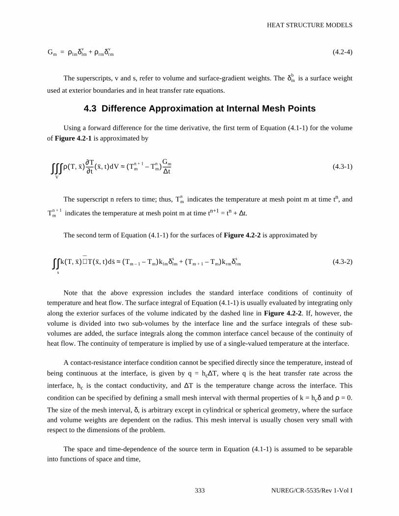
HEAT STRUCTURE MODELS
(4.2-4)
The superscripts, v and s, refer to volume and surface-gradient weights. The is a surface weight
used at exterior boundaries and in heat transfer rate equations.
4.3 Difference Approximation at Internal Mesh Points
Using a forward difference for the time derivative, the first term of Equation (4.1-1) for the volume
of Figure 4.2-1 is approximated by
(4.3-1)
The superscript n refers to time; thus, indicates the temperature at mesh point m at time tn, and
indicates the temperature at mesh point m at time tn+1 = tn + ∆t.
The second term of Equation (4.1-1) for the surfaces of Figure 4.2-2 is approximated by
(4.3-2)
Note that the above expression includes the standard interface conditions of continuity of
temperature and heat flow. The surface integral of Equation (4.1-1) is usually evaluated by integrating only
along the exterior surfaces of the volume indicated by the dashed line in Figure 4.2-2. If, however, the
volume is divided into two sub-volumes by the interface line and the surface integrals of these sub-
volumes are added, the surface integrals along the common interface cancel because of the continuity of
heat flow. The continuity of temperature is implied by use of a single-valued temperature at the interface.
A contact-resistance interface condition cannot be specified directly since the temperature, instead of
being continuous at the interface, is given by q = hc∆T, where q is the heat transfer rate across the
interface, hc is the contact conductivity, and ∆T is the temperature change across the interface. This
condition can be specified by defining a small mesh interval with thermal properties of k = hcδ and ρ = 0.
The size of the mesh interval, δ, is arbitrary except in cylindrical or spherical geometry, where the surface
and volume weights are dependent on the radius. This mesh interval is usually chosen very small with
respect to the dimensions of the problem.
The space and time-dependence of the source term in Equation (4.1-1) is assumed to be separable
into functions of space and time,
Gm ρlmδlmv ρrmδrm
v+=
δmb
ρ T x,( )∂T∂t------ x t,( )dV Tm
n 1+ Tmn–( )
Gm
∆t-------≈∫
V
∫∫
Tmn
Tmn 1+
k T x,( )∇ T x t,( )ds Tm 1– Tm–( )klmδlms Tm 1+ Tm–( )krmδrm
s+≈s
∫∫
333 NUREG/CR-5535/Rev 1-Vol I
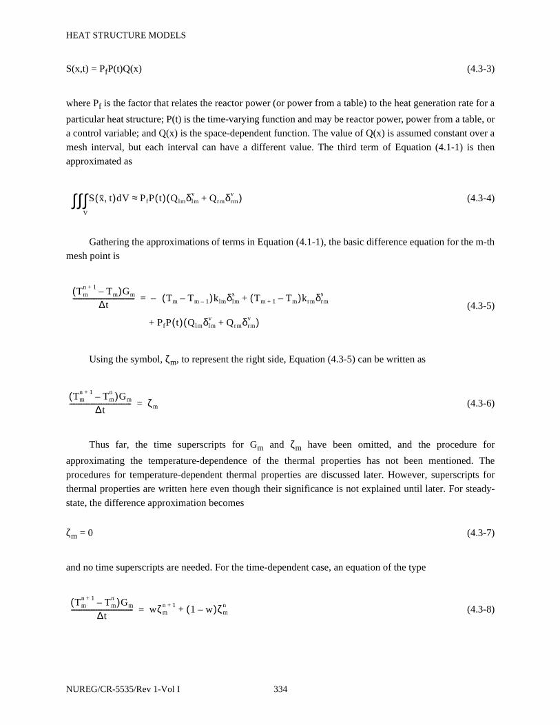
HEAT STRUCTURE MODELS
S(x,t) = PfP(t)Q(x) (4.3-3)
where Pf is the factor that relates the reactor power (or power from a table) to the heat generation rate for a
particular heat structure; P(t) is the time-varying function and may be reactor power, power from a table, or
a control variable; and Q(x) is the space-dependent function. The value of Q(x) is assumed constant over a
mesh interval, but each interval can have a different value. The third term of Equation (4.1-1) is then
approximated as
(4.3-4)
Gathering the approximations of terms in Equation (4.1-1), the basic difference equation for the m-th
mesh point is
(4.3-5)
Using the symbol, ζm, to represent the right side, Equation (4.3-5) can be written as
(4.3-6)
Thus far, the time superscripts for Gm and ζm have been omitted, and the procedure for
approximating the temperature-dependence of the thermal properties has not been mentioned. The
procedures for temperature-dependent thermal properties are discussed later. However, superscripts for
thermal properties are written here even though their significance is not explained until later. For steady-
state, the difference approximation becomes
ζm = 0 (4.3-7)
and no time superscripts are needed. For the time-dependent case, an equation of the type
(4.3-8)
S x t,( )dV PfP t( ) Qlmδlmv Qrmδrm
v+( )≈V
∫∫∫
Tmn 1+ Tm–( )Gm
∆t------------------------------------- – Tm Tm 1––( )klmδlm
s Tm 1+ Tm–( )krmδrms+=
PfP t( ) Qlmδlmv Qrmδrm
v+( )+
Tmn 1+ Tm
n–( )Gm
∆t------------------------------------- ζm=
Tmn 1+ Tm
n–( )Gm
∆t------------------------------------- wζm
n 1+ 1 w–( )ζmn+=
NUREG/CR-5535/Rev 1-Vol I 334
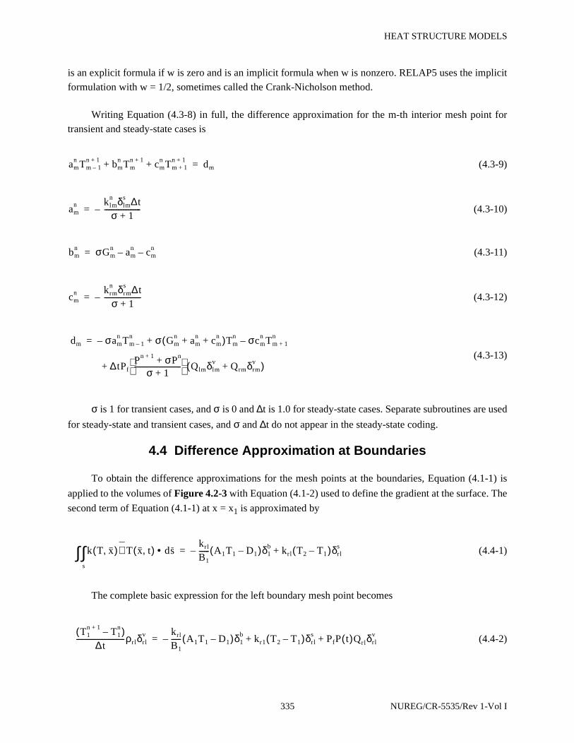
HEAT STRUCTURE MODELS
is an explicit formula if w is zero and is an implicit formula when w is nonzero. RELAP5 uses the implicit
formulation with w = 1/2, sometimes called the Crank-Nicholson method.
Writing Equation (4.3-8) in full, the difference approximation for the m-th interior mesh point for
transient and steady-state cases is
(4.3-9)
(4.3-10)
(4.3-11)
(4.3-12)
(4.3-13)
σ is 1 for transient cases, and σ is 0 and ∆t is 1.0 for steady-state cases. Separate subroutines are used
for steady-state and transient cases, and σ and ∆t do not appear in the steady-state coding.
4.4 Difference Approximation at Boundaries
To obtain the difference approximations for the mesh points at the boundaries, Equation (4.1-1) is
applied to the volumes of Figure 4.2-3 with Equation (4.1-2) used to define the gradient at the surface. The
second term of Equation (4.1-1) at x = x1 is approximated by
(4.4-1)
The complete basic expression for the left boundary mesh point becomes
(4.4-2)
amn Tm 1–
n 1+ bmn Tm
n 1+ cmn Tm 1+
n 1++ + dm=
amn
klmn δlm
s ∆tσ 1+
---------------------–=
bmn σGm
n amn– cm
n–=
cmn
krmn δrm
s ∆tσ 1+
---------------------–=
dm σamn Tm 1–
n– σ Gmn am
n cmn+ +( )Tm
n σcmn Tm 1+
n–+=
∆tPfPn 1+ σPn+
σ 1+---------------------------
Qlmδlmv Qrmδrm
v+( )+
k T x,( )∇ T x t,( ) ds•s
∫∫krl
B1------ A1T1 D1–( )δ1
b– krl T2 T1–( )δrls+=
T1n 1+ T1
n–( )∆t
----------------------------ρrlδrlv krl
B1------ A1T1 D1–( )δ1
b– kr1 T2 T1–( )δrls PfP t( )Qrlδrl
v+ +=
335 NUREG/CR-5535/Rev 1-Vol I
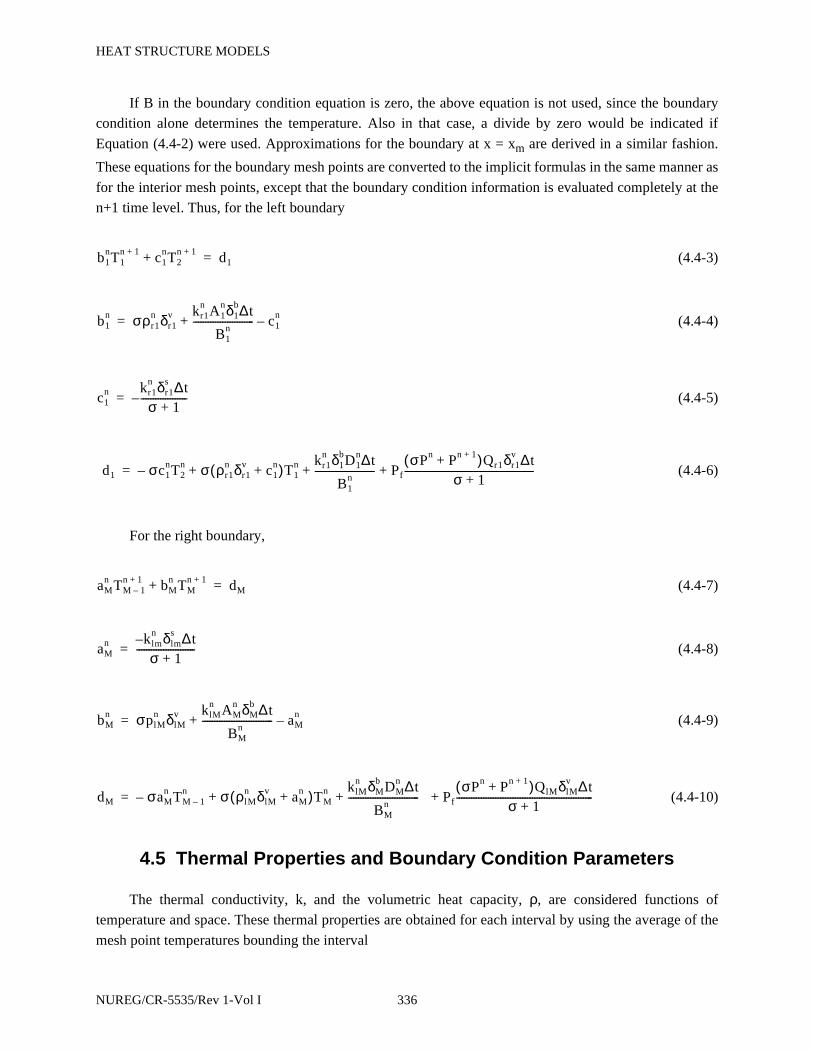
HEAT STRUCTURE MODELS
If B in the boundary condition equation is zero, the above equation is not used, since the boundary
condition alone determines the temperature. Also in that case, a divide by zero would be indicated if
Equation (4.4-2) were used. Approximations for the boundary at x = xm are derived in a similar fashion.
These equations for the boundary mesh points are converted to the implicit formulas in the same manner as
for the interior mesh points, except that the boundary condition information is evaluated completely at the
n+1 time level. Thus, for the left boundary
(4.4-3)
(4.4-4)
(4.4-5)
(4.4-6)
For the right boundary,
(4.4-7)
(4.4-8)
(4.4-9)
(4.4-10)
4.5 Thermal Properties and Boundary Condition Parameters
The thermal conductivity, k, and the volumetric heat capacity, ρ, are considered functions of
temperature and space. These thermal properties are obtained for each interval by using the average of the
mesh point temperatures bounding the interval
b1nT1
n 1+ c1nT2
n 1++ d1=
b1n σρr1
n δr1v kr1
n A1nδ1
b∆t
B1n
------------------------- c1n–+=
c1n kr1
n δr1s ∆t
σ 1+-------------------–=
d1 σc1nT2
n– σ ρr1n δr1
v c1n+( )T1
n kr1n δ1
bD1n∆t
B1n
------------------------- Pf
σPn Pn 1++( )Qr1δr1v ∆t
σ 1+-----------------------------------------------------+ + +=
aMn TM 1–
n 1+ bMn TM
n 1++ dM=
aMn klm
n δlms ∆t–
σ 1+------------------------=
bMn σplM
n δlMv klM
n AMn δM
b ∆t
BMn
----------------------------- aMn–+=
dM σaMn TM 1–
n– σ ρlMn δlM
v aMn+( )TM
n klMn δM
b DMn ∆t
BMn
----------------------------- P+ f
σPn Pn 1++( )QlMδlMv ∆t
σ 1+--------------------------------------------------------+ +=
NUREG/CR-5535/Rev 1-Vol I 336

HEAT STRUCTURE MODELS
(4.5-1)
(4.5-2)
The quantity, ρ, is treated in the same manner. The boundary condition parameters, A, B, and D, are
considered functions of temperature and time.
4.6 RELAP5 Specific Boundary Conditions
The development of the difference equations uses a general form for the boundary conditions and the
specific conditions implemented in RELAP5 are expressed in that form. For heat structure boundaries
attached to hydrodynamic volumes, a convective package is typically used to define the boundary
conditions. In addition, symmetry or insulated conditions are provided, and for special situations, tabular
based conditions can be specified.
4.6.1 Correlation Package Conditions
The correlation package partitions the total heat flux at the heat structure surface into heat fluxes
from or to the liquid and vapor phases. The heat fluxes are defined using five heat transfer coefficients and
four fluid temperatures.
qf = hff[Tsr - Tf] + hfT[Tsr - Ts(P)] (4.6-1)
qg = hgg[Tsr - Tg] + hgT[Tsr - Ts(P)] +hgp[Tsr - T
s(Ps)] (4.6-2)
qb = qf + qg (4.6-3)
where
qf = heat flux to liquid
qg = heat flux to vapor
qb = total heat flux
Tsr = surface temperature
Tf = liquid temperature
kl m, kTm 1– Tm+
2-------------------------
kr m 1–,= =
kr m, kTm Tm 1++
2--------------------------
kl m 1+,= =
337 NUREG/CR-5535/Rev 1-Vol I

HEAT STRUCTURE MODELS
Tg = vapor temperature
hff = heat transfer coefficient for difference of surface temperature and liquid
temperature for heat transfer to liquid
hfT = heat transfer coefficient for difference of surface temperature and saturation
temperature corresponding to total pressure for heat transfer to liquid
hgg = heat transfer coefficient for difference of surface temperature and vapor
temperature for heat transfer to vapor
hgT = heat transfer coefficient for difference of surface temperature and saturation
temperature corresponding to total pressure for heat transfer to vapor
hgp = heat transfer coefficient for difference of surface temperature and saturation
temperature corresponding to partial pressure of water vapor for transfer tovapor
Using first order Taylor series approximations,
(4.6-4)
(4.6-5)
where ∆ is an operator, ∆F = Fn+1 - Fn.
Note that and are not old-time values of heat fluxes but instead are the heat fluxes obtained
from the correlations using old-time surface temperature and fluid conditions. Because only new-time
boundary condition information is used in the difference equations, the old-time heat fluxes do not appear
in the difference equations.
Assuming the heat transfer coefficients are constant over a time step,
(4.6-6)
(4.6-7)
qfn 1+ qf
0 ∂qf
∂Tsr----------∆Tsr
∂qf
∂Tf--------∆Tf
∂qf
∂TT---------∆Ts P( )+ + +=
qgn 1+ qg
0 ∂qg
∂Tsr----------∆Tsr
∂qg
∂Tg---------∆Tg
∂qg
∂Ts P( )-----------------∆Ts P( )
∂qg
∂Ts Ps( )------------------∆Ts Ps( )+ + + +=
qf0 qg
0
∂qf
∂Tsr---------- hff hfT+=
∂qf
∂Tf-------- hff–=
NUREG/CR-5535/Rev 1-Vol I 338

HEAT STRUCTURE MODELS
(4.6-8)
(4.6-9)
(4.6-10)
(4.6-11)
(4.6-12)
Then,
(4.6-13)
(4.6-14)
(4.6-15)
where
hb = hff + hfT + hgg + hgT + hgp (4.6-16)
Expressing Equation (4.6-15) in terms of the general boundary condition,
A = -hb (4.6-17)
B = -k (4.6-18)
(4.6-19)
∂qf
∂TT--------- hfT–=
∂qg
∂Tsr---------- hgg hgT hgp+ +=
∂qg
∂Tg--------- hgg–=
∂qg
∂TT--------- hgT–=
∂qg
∂Tp--------- hgp–=
qfn 1+ qf
0 hff hfT+[ ]∆ Tsr hff∆Tf– hfT∆Ts P( )–+=
qgn 1+ qg
0 hgg hgT hgp+ +[ ]∆ Tsr hgg∆Tg– hgT∆Ts P( )– hgp∆Ts Ps( )–+=
qbn 1+ qf
0 qg0 hb∆Tsr hff∆Tf– hgg∆Tg– hfT hgT+[ ]∆ Ts P( ) hgp∆Ts Ps( )––+ +=
D qf0 qg
0 hb∆Tsr hff∆Tf– hgg∆Tg– hfT hgT+[ ]∆ Ts P( )– hgp∆Ts Ps( )–+ +=
339 NUREG/CR-5535/Rev 1-Vol I

HEAT STRUCTURE MODELS
4.6.2 Insulated and Tabular Boundary Conditions
The other boundary conditions implemented in RELAP5 are given below. The first two conditions
are flux-specified conditions; the first condition is a symmetry or insulated condition and is just a special
case of the second condition. The third condition is a convection condition similar to that used with the
correlation package except that only a total heat transfer coefficient which is a tabular function of time or
surface temperature is used. The last condition directly specifies the surface temperature.
(4.6-20)
(4.6-21)
(4.6-22)
T=TTA(t) (4.6-23)
where
qTA = the total heat flux as a function of time obtained from input tables
hTA = the total heat transfer coefficient as an input tabular function of either time or
surface temperature
TTA = either an input tabular function of time or the void fraction weighted average
of the liquid and vapor temperatures of the hydrodynamic volume attached tothe boundary
4.7 Solution of Simultaneous Equations
The difference approximation for the mesh points [Equation (4.3-9), (4.4-3), and (4.4-7)] lead to a
tridiagonal set of M equations.
k∂T∂x------– 0=
k∂T∂x------– qTA t( )=
k∂T∂x------– hTA T TTA–( )=
NUREG/CR-5535/Rev 1-Vol I 340

HEAT STRUCTURE MODELS
(4.7-1)
Equations 1 and M correspond to the left and right boundary mesh points respectively, and equations
2 through M-1 correspond to the interior mesh points. The terms in d2 through dM-1 do not include any of
the fluid or saturation temperatures, Tf, Tg, Ts(P), and Ts(Ps). But
d1 = d10 + d11∆T1f + d1g∆T1g + d1T + d1p (4.7-2)
dM = dM10 + dMf∆TMf + dMg∆TMg + dMT + dMp (4.7-3)
where the first subscript, 1 or M, has been introduced to indicate the left or right boundary. The coefficient
matrix is symmetric unless a boundary condition specifies the surface temperature. In that case, the
corresponding off-diagonal element is zero and thus symmetry may not exist in the first and/or last rows.
The solution to the above equation is obtained by
(4.7-4)
and for j = 2, 3,..., M-1 (4.7-5)
(4.7-6)
gj = -Ejgj+1 + Fj for j = M-1, M-2,..., 3, 2, 1 (4.7-7)
for all j (4.7-8)
These procedures can be derived by applying the rules for Gaussian elimination. This method of
solution introduces little roundoff error if the off-diagonal elements are negative and the diagonal is greater
b1 c1
a2 b2 c2
• •• • •
aM 1– bM 1– cM 1–
aM bM
T1
T2
••
TM 1–
TM
d1
d2
••
dM 1–
dM
=
∆T1s P( ) ∆T1
s Ps( )
∆TMs P( ) ∆TM
s Ps( )
E1
c1
b1----- and F1
d1
b1-----= =
Ej
cj
bj ajEj 1––-------------------------= Fj
dj ajFj 1––bj ajEj 1––-------------------------=
gM
dM aMFM 1––bM aMEM 1––--------------------------------=
Tjn 1+ gj=
341 NUREG/CR-5535/Rev 1-Vol I
HEAT STRUCTURE MODELS
than the sum of the magnitudes of the off-diagonal elements. From the form of the difference equations,
these conditions are satisfied for any values of the mesh point spacing, time step, and thermal properties.
Expanding the expression for ,
(4.7-9)
For the g factors, the first subscript indicates the mesh point number, the second subscript indicates
the boundary, and the third subscript indicates the particular fluid temperature.
A user option allows an explicit or an implicit coupling between the heat conduction-transfer and
hydrodynamic time advancements. With the explicit option, the changes in hydrodynamic temperatures are
assumed zero at this point and the new-time temperatures are given by the first term of Equation (4.7-9). If
the implicit advancement is used, the final temperatures are computed using Equation (4.7-9) after the fluid
temperatures are computed.
4.8 Computation of Heat Fluxes
When the correlation boundary condition package is used, the new-time heat fluxes to the liquid and
vapor phases are computed by substituting the Equation (4.7-9) for the surface temperature into the
boundary conditions given in Equation (4.6-1) and (4.6-2). The expression for any temperature could
involve the fluid temperatures from both the left and right boundary volumes. If only one side of the heat
structure is attached to a hydrodynamic volume, that boundary condition would involve only those volume
conditions. That fits in well with the numerical approximations in the hydrodynamic solution which
assume the conservations equations for each volume include new time values only from that volume. Most
heat structures such as fuel pins or plates and piping have only one side connected to a hydrodynamic
volume. An important case where the two sides are connected to two different volumes is a heat structure
representing heat exchanger tubing. This situation would involve unknown temperatures from more than
one volume in the energy equations for each attached volume and thus would not be compatible with the
hydrodynamic advancement scheme. To avoid this problem, the heat flux for one boundary ignores the
effects of fluid temperature changes in the other volume. This is a reasonable approximation since the
effects of temperature changes of the fluid on one side of the heat structure has a highly attenuated effect
on the heat flux on the other side.
Dropping the subscript for the particular surface, the expressions for heat fluxes are
(4.8-1)
Tjn 1+
Tjn 1+ gj0 gj1f∆T1f gj1g∆T1g gj1T∆T1
s P( ) gj1p∆T1s Ps( )+ + + +=
gjMf∆TMf gjMg∆TMg gjMT∆TMs P( ) gjMp∆TM
s Ps( ) + + + +
qfn 1+ qf
0 hff hfT+[ ] g0 Tsrn–[ ]+ + hff hfT+[ ] gf∆Tf gg∆Tg gT∆Ts P( ) gp∆Ts Ps( )+ ++[ ]=
hff∆Tf– hfT∆Ts P( )– qf0 qff∆Tf qfg∆Tg qfT∆Ts P( ) + + +=
NUREG/CR-5535/Rev 1-Vol I 342
HEAT STRUCTURE MODELS
(4.8-2)
The expression following the second equal sign in the equations above is a convenient gathering of
terms for passing heat flux information to the hydrodynamic advancement. The coefficients of the fluid
temperature changes are zero if the explicit coupling between the heat conduction-transfer and
hydrodynamics is used.
For heat fluxes from boundaries not using the correlation package, a total heat flux is computed and
distributed to the liquid and vapor phases in direct proportion to their void fractions. The heat fluxes are
returned in qf0 and qg0, and the coefficients of the fluid temperature changes are set to zero. For flux
specified conditions, the total heat flux is given directly by the boundary condition. For a convection
boundary, the total heat flux is obtained by substituting in the surface temperature. If the other boundary
uses the convective package, the surface temperature is that assuming the fluid temperature changes are
zero. For the temperature-specified boundary, the heat flux is computed from the boundary difference
equation (even though it was not used to compute the temperature). The expression for the right boundary
(the left is similar) is
(4.8-3)
4.9 Two-Dimensional Conduction Solution/Reflood
A two-dimensional conduction scheme is used in the reflood model for cylindrical or rectangular
heat structures. Figure 4.9-1 shows an elemental cell around the mesh point. For a cylindrical geometry,
the volume elements are
(4.9-1)
(4.9-2)
qgn 1+ qg
0 hgf hgT hgp∆Ts Ps( )+ +[ ] g0 Tsrn–[ ]+ +=
hgg hgT hgp+ +[ ] gf∆Tf gg∆Tg gT∆Ts P( ) gp∆Ts Ps( )+ ++[ ]
hgg∆Tg– hgt∆Ts P( )– hgp∆Ts Ps( )– qg0 qgf∆Tf qgg∆Tg qgT∆Ts P( ) qgp∆Ts Ps( ) + + + +=
qMn 1+ δ1M
n k1Mn
σ 1+------------- TM 1–
n 1+ TMn 1+–( )δ1M
s σk1Mn
σ 1+------------- TM 1–
n TMn–( )δ1M
s+=
PfσPn Pn 1++( )
σ 1+--------------------------------Q1Mδ1M
v σρ1Mn
∆t------------- TM
n 1+ TMn–( )δ1M
v–+
V1 πδtδ1
ri
δ1
4-----–
2--------------
=
V2 πδtδr
ri
δr
4----+
2--------------
=
343 NUREG/CR-5535/Rev 1-Vol I
HEAT STRUCTURE MODELS
(4.9-3)
(4.9-4)
and the surface elements are
(4.9-5)
Figure 4.9-1 Volume and Surface Elements Around a Mesh Point (i, j)
δl
V3 V4
X (i, j-1)
A5A6
(i, j)
A7 A4
A2A1
(i+1, j)
A8 A3
(i, j-+1)X
(i-1, j)XX X
V1 V2
r
z
2δb2
δt2
δr2
V3 πδbδ1
ri
δ1
4-----–
2--------------
=
V4 πδbδr
ri
δr
4----+
2--------------
=
A1 πδ1 ri
δl
4----–
=
NUREG/CR-5535/Rev 1-Vol I 344
HEAT STRUCTURE MODELS
(4.9-6)
(4.9-7)
(4.9-8)
A5 = A2 (4.9-9)
A6 = A1 (4.9-10)
(4.9-11)
(4.9-12)
Integration of the heat conduction Equation (4.1-1) over the elemental cell yields the following form
of finite difference equation
(4.9-13)
By defining the material properties, ρij and kij, at the center of the r-direction interval between mesh
points (ij) and (i + 1,j), the coefficients Gij, and of Equation (4.9-13) can be written as
Gij = ρi-1,j (V1 + V3) + ρij (V2 + V4) (4.9-14)
(4.9-15)
(4.9-16)
A2 πδr ri
δr
4----+
=
A3 πδt ri
δr
2----+
=
A4 πδb ri
δr
2----+
=
A7 πδb ri
δl
2----–
=
A8 πδt ri
δl
2----–
=
Gij
Ti j,n 1+ Ti j,
n–∆t
------------------------- ai j,
L Ti 1 j,– aijRTi 1 j,+ aij
TTi j 1+, aijBTi j 1–,+ + +=
aijL aij
R aijB aij
T+ + +( )Tij– Sij +
aijR aij
T
aijR kij A3 A4+( )
δr------------------------------=
aijT
kij ki j 1+,+( )A2
2------ ki 1 j,– ki 1 j 1+,–+( )
A1
2------+
δt---------------------------------------------------------------------------------------------------=
345 NUREG/CR-5535/Rev 1-Vol I
HEAT STRUCTURE MODELS
The other two coefficients, and , are obtained by the symmetry relations
(4.9-17)
(4.9-18)
The space and time-dependence of the source term, S, described in Equation (4.3-3) are extended to
the two-dimensional cases as
S = Pf P(t) Q (r,z) (4.9-19)
with the assumption that Q is independent of z within a heat structure. Accordingly, the heat source term Sij
of Equation (4.9-13) is
(4.9-20)
Here, and if the entire cell is within the same heat structure.
Equation (4.9-13) is written for an interior point (ij). For a point on the boundary, some of the
coefficients , , , and should vanish. For example, at the bottom corner, and are zero.
Also some of the terms in Equation (4.9-16) and (4.9-20) disappear. Furthermore, the boundary condition
must be added. To be consistent with the one-dimensional heat conduction scheme, an assumption is made
that no heat is fluxed across the top and bottom ends. For the right and left boundaries, the boundary
condition can be represented by one of the forms described in Equation (4.6-1), (4.6-2), and (4.6-20)
through (4.6-22). The boundary condition specifying the surface temperature as a function of time,
Equation (4.6-23), has been dropped in the two-dimensional scheme for computational efficiency.
The two-dimensional capability currently uses only explicit coupling between the heat conduction-
transfer and hydrodynamics.
The difference Equation (4.9-13) is solved using the alternating direction implicit (ADI) method. The
scheme is represented by two steps as follows:
1. Column Inversion:
aijL aij
B
aijL ai 1 j,–
R=
aijB ai j 1–,
T=
Sij PfP t( ) QTV1 QBV3 QrTV2 Qr
BV4+ + +( )=
QlT Ql
B= QrT Qr
B=
aijL aij
R aijB aij
T aijL aij
B
NUREG/CR-5535/Rev 1-Vol I 346

HEAT STRUCTURE MODELS
(4.9-21)
2. Row Inversion:
(4.9-22)
Here the superscripts n, n + 1/2, and n + 1 denote the values at times t, t + ∆t/2, and t + ∆t,
respectively.
4.10 Fine Mesh Rezoning Scheme
A fine mesh-rezoning scheme is implemented to efficiently use the two-dimensional conduction
solution for reflood calculations. The scheme is similar to the one used in COBRA-TF4.10-1 and is intended
to resolve the large axial variation of wall temperatures and heat fluxes. The number of axial nodes in the
heat structures is varied in such a way that the fine nodes exist only in the nucleate boiling and transition
boiling regions.
A heat-structure geometry, which is composed of 1 to 99 heat structures as specified by users, is
selected as an elementary unit for the reflood model. Figure 4.10-1a shows a typical heat structure
geometry with one fluid-control volume connected to each heat structure. The dots are radial mesh points.
At the initiation of the reflood model, each heat structure is subdivided into two axial intervals (Figure
4.10-2b). A two-dimensional array of mesh points is thus formed. Thereafter, the number of axial intervals
may be doubled, halved, or unchanged at each time step according to a set of rules to be discussed in the
next paragraph. Figure 4.10-2 also shows an example of a heat structure going through a cycle of axial
nodalization variation.
The number of axial mesh intervals in a heat structure depends on the heat-transfer regimes in the
heat structures. At each time step, all heat structures in a heat-structure geometry are searched to find the
positions of TCHF, the wall temperature where critical heat flux occurs, TQ, the quench or rewetting
temperature, and TIB, the wall temperature at the incipience of boiling. Let us assume that TIB, TCHF, and
TQ are at the i-, j-, and k-th heat structures and k > j > i. Also, let N be the maximum number of axial mesh
Tijn 1 2⁄+ Tij
n–( )Gij
∆t2-----
---------------------------------------- aij
LTi 1 j,–n aij
RTi 1 j,+n aij
BTi j 1–,n 1 2⁄+ aij
TTi j 1+,n 1 2⁄++ + +=
aijL aij
R+( )– Tijn aij
T aijB+( )Tij
n 1 2⁄+– Sij .+
Tijn 1+ Tij
n 1 2⁄+–( )Gij
∆t2-----
---------------------------------------------- aij
LTi 1 j,–n 1+ aij
RTi 1 j,+n 1+ aij
BTi j 1–,n 1 2⁄+ aij
TTi j 1+,n 1 2⁄++ + +=
aijL aij
R+( )Tijn 1+– aij
T aijB+( )Tij
n 1 2⁄+– Sij +
347 NUREG/CR-5535/Rev 1-Vol I

HEAT STRUCTURE MODELS
intervals specified by the user and αg be the void fraction in the connected control volume. The number of
axial mesh intervals in a heat structure is determined according to the following rules:
• For αg > 0.999 or αg = 0, the number is halved but not less than 2.
• For the (k + 1)-th heat structure, the number is doubled but not greater than N/2.
• For the (i - 1)-th heat structure, the number is halved but not less than N/2.
• The number is doubled up to N for the heat structures between max (j + 1, k) and min (j-, i) and in the region of maximum wall temperature gradient.
• For all other heat structures, the number is unchanged.
Figure 4.10-1 An Elementary Heat Structure Unit for Reflood
n-1
n
2
1
a b
NUREG/CR-5535/Rev 1-Vol I 348

HEAT STRUCTURE MODELS
4.10.1 References
4.10-1. J. M. Kelly. “Quench Front Modeling and Reflood Heat Transfer in COBRA-TF.” ASME WinterAnnual Meeting. New York, NY. 1979. 79-WA/HT-63.
4.11 Gap Conductance Model
The RELAP5 dynamic gap conductance model defines an effective gap conductivity based on a
simplified deformation model generated from FRAP-T6.4.11-1 The model employs three assumptions as
follows: (a) the fuel-to-cladding radiation heat transfer, which only contributes significantly to the gap
conductivity under the conditions of cladding ballooning, is neglected unless the cladding deformation
model is activated (see Section 4.14), (b) the minimum gap size is limited such that the maximum effective
gap conductivity is about the same order as that of metals; (c) the direct contact of the fuel pellet and the
cladding is not explicitly considered.
Figure 4.10-2 An Example of the fine Mesh-Rezoning Process
X X X
X X XX X XX X X
1-D conduction
Start of reflood
HalvedDoubled
Maximum axial nodes
Doubled Halved
349 NUREG/CR-5535/Rev 1-Vol I

HEAT STRUCTURE MODELS
The gap conductance through the gas is inversely proportional to the size of the gap. Since the
longitudinal axis of the fuel pellets is usually offset from the longitudinal axis of the cladding, the width of
the fuel-cladding gap varies with circumferential position. This variation causes the conductance through
the gas in the fuel-cladding gap to vary with circumferential position. The circumferential variation of the
conductance is taken into account by dividing the gap into several equal length segments, as shown in
Figure 4.11-1. The conductance for each segment is calculated and then an average conductance, hg, is
computed in the FRAP-T6 model by the equation
(4.11-1)
where
hg = conductance through the gas in the gap (W/m2•K)
n = number of a circumferential segment
N = total number of circumferential segments = 8
Figure 4.11-1 Segmentation at the Fuel-Cladding Gap
Line of symmetry
Fuel-claddinggap
Fuelcrack
Segment n
Segment 1
Fuelpellet
Cladding
hg
kg
N-----
1tn 3.2 RF Rc+( ) g1 g2+( )+ +---------------------------------------------------------------------
n 1=
N
∑=
NUREG/CR-5535/Rev 1-Vol I 350
HEAT STRUCTURE MODELS
kg = thermal conductivity of gas (W/m•K)
tn = width of fuel-cladding gap at the midpoint of the n-th circumferential segment
(m)
RF = surface roughness of the fuel (m)
Rc = surface roughness of the cladding (m)
g1,g2 = temperature jump distance terms for fuel and cladding
The width of the fuel-cladding gap at any given circumferential segment is calculated by the equation
(4.11-2)
where
tg = circumferentially averaged fuel-cladding gap width (m)
to = as-fabricated fuel-cladding gap width (m)
The value of tn in Equation (4.11-2) is limited between zero and 2tg.
The temperature jump distance terms account for the temperature discontinuity caused by incomplete
thermal accommodation of gas molecules to the surface temperature. The terms also account for the
inability of gas molecules leaving the fuel and cladding surfaces to completely exchange their energy with
neighboring gas molecules, which produces a nonlinear temperature gradient near the fuel and cladding
surfaces. The terms are calculated by
(4.11-3)
where
Tg = temperature of gas in the fuel-cladding gap (K)
Pg = gas pressure (Pa)
fi = mole fractions of i-th component of gas
tn tg 1–2n 1–
N---------------
+ to+=
g1 g2+0.024688kgTg
1 2⁄
Pg fiaiMi1 2⁄–
i
∑--------------------------------------=
351 NUREG/CR-5535/Rev 1-Vol I
HEAT STRUCTURE MODELS
ai = accommodation coefficient of the i-th component of gas
Mi = molecular weight of the i-th component of gas
The accommodation coefficients for helium and xenon are obtained by using curve fits to the data of
Ullman:4.11-2
aHe = 0.425 - 2.3 x 10⁻⁴ Tg (helium) (4.11-4)
aXe = 0.740 - 2.5 x 10⁻⁴ Tg (xenon) (4.11-5)
If Tg is > 1,000 K, Tg is set to 1,000 K. The accommodation coefficients for other gases are
determined by interpolation and written as
(4.11-6)
The circumferential averaged width of the fuel cladding gap, tg, in Equation (4.11-2) is determined
by the expression
tg = to - uF + uC (4.11-7)
where
uF = radial displacement of the fuel pellet surface (m)
uC = radial displacement of cladding inner surface (m)
The radial displacements, uF and uC, are primarily due to thermal expansion. The radial
displacement, of the fuel pellet surface, uF, is calculated by the equation
uF = uTF + ur + us (4.11-8)
where
uTF = radial displacement due to thermal expansion (m)
ur = radial displacement due to uniform fuel relocation (m)
ai aHe
Mi MHe–( )MXe MHe–( )
------------------------------- aXe aHe–( )+=
NUREG/CR-5535/Rev 1-Vol I 352

HEAT STRUCTURE MODELS
us = radial displacement due to fission gas induced fuel swelling and densification
(m)
In the RELAP5 model, the variable ur is assumed to be zero. The value of the variable us is supplied
by the user. The fuel thermal expansion is obtained from the equation
(4.11-9)
where
n = radial mesh point number
N = total number of mesh points in the fuel
rn = radius of radial mesh point n
εTF = function defining thermal expansion of fuel as a function of temperature
Tn+1/2 = average fuel temperature at the center of the node between mesh points n and
n+1
The radial displacement of the inner surface of the cladding is calculated by
uc = uTC + ucc + ue (4.11-10)
where
uTC = radial displacement due to thermal expansion (m)
ucc = radial displacement due to cladding creepdown (m)
ue = radial displacement due to elastic deformation (m)
The value of ucc must be supplied by the user. For beginning-of-life fuel rods, ucc is equal to zero.
For fuel rods with a significant amount of burnup, a FRAPCON-24.11-3 analysis is required to determine
the value of ucc. The thermal expansion, uTC, is obtained from
uTC = rcm εTC (Tc) (4.11-11)
uTF rn rn 1––( )εTF Tn 1 2⁄+( )n 2=
N
∑=
353 NUREG/CR-5535/Rev 1-Vol I

HEAT STRUCTURE MODELS
where
rcm = radius of midplane of cladding (m)
εTC = function defining thermal expansion of cladding as a function of temperature
Tc = temperature of cladding at midplane (K)
The elastic deformation, ue, is calculated by
(4.11-12)
where
E = Young’s modulus for the cladding (Pa)
σh = cladding hoop stress (Pa)
σz = cladding axial stress (Pa)
ν = Poisson’s ratio for the cladding
The cladding hoop and axial stress are given by
(4.11-13)
(4.11-14)
where
Pf = coolant pressure (Pa)
ri = inner radius of cladding (m)
ro = outer radius of cladding (m)
The Poisson’s ratio used is
ue rcm
σh νσz–E
-------------------- =
σn
Pgri Pfro–ro ri–
------------------------=
σz
Pgri2 Pfro
2–
ro2 ri
2–-------------------------=
NUREG/CR-5535/Rev 1-Vol I 354

HEAT STRUCTURE MODELS
ν = 0.3 . (4.11-15)
The internal gas pressure Pg is determined in FRAP-T64.11-1 by a detailed plenum model. Since a
plenum model is not included in the simplified approach, a static-ideal gas approximation for a fixed-
plenum volume is used to calculate Pg, i.e.,
(4.11-16)
where
Pg,i = initial gas pressure in the gap (Pa)
Tf,i = initial coolant temperature at the top of the core (K)
Tf = current coolant temperature at the top of the core (K)
The initial internal gas pressure must be supplied by the user.
The volumetric heat capacity and thermal conductivity of the fuel rod materials, except for the
thermal conductivity of the gap gas, must be supplied by the user. For the computation of the gas thermal
conductivity, the user is required to provide the gas composition in terms of the mole fractions of seven
common gases included in the model. The properties for determining material thermal expansion and
elastic deformation are calculated from permanent data within the code, and no user-input is needed. The
user, however, should be aware that these properties are computed under the assumption that the fuel
material is uranium oxide and the cladding material is zircaloy. The properties of U02 and zircaloy along
with gas conductivity are taken from MATPRO-11 (Revision 2)4.11-4 and are described below.
The conductivity as a function of temperature for a pure noble or diatomic gas is calculated using
(4.11-17)
The constants A and B for seven common gases are given in Table 4.11-1. The thermal conductivity
of a gas mixture is calculated from the expression
(4.11-18)
Pg Pg i,Tf
Tf i,--------=
kg ATgB=
kg
kiXi
Xi Φi jXj
j 1=
N
∑+
---------------------------------
i 1=
N
∑=
355 NUREG/CR-5535/Rev 1-Vol I
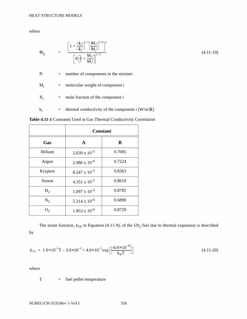
HEAT STRUCTURE MODELS
where
Φij = (4.11-19)
N = number of components in the mixture
Mi = molecular weight of component i
Xi = mole fraction of the component i
ki = thermal conductivity of the component i (W/m⋅K)
The strain function, εTF in Equation (4.11-9), of the U02 fuel due to thermal expansion is described
by
(4.11-20)
where
T = fuel pellet temperature
Table 4.11-1 Constants Used in Gas Thermal Conductivity Correlation
Constant
Gas A B
Helium 2.639 x 10⁻³ 0.7085
Argon 2.986 x 10⁻⁴ 0.7224
Krypton 8.247 x 10⁻⁵ 0.8363
Xenon 4.351 x 10⁻⁵ 0.8618
H2 1.097 x 10⁻³ 0.8785
N2 5.314 x 10⁻⁴ 0.6898
O2 1.853 x 10⁻⁴ 0.8729
1ki
kj----
1 2⁄ Mi
Mj------
1 4⁄
+2
8 1Mi
Mj------+
1 2⁄----------------------------------------------------
εTF 1.0 5–×10 T 3.0 3–×10– 4.0 2–×106.9 20–×10–
kBT--------------------------
exp+=
NUREG/CR-5535/Rev 1-Vol I 356
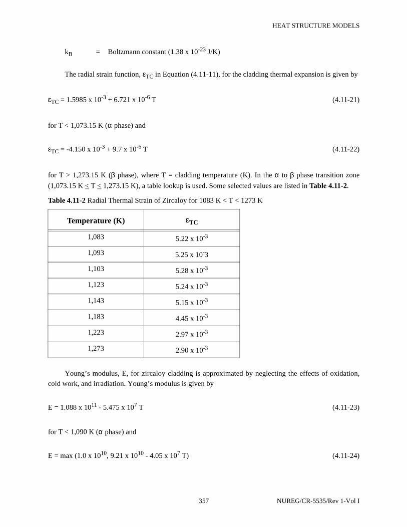
HEAT STRUCTURE MODELS
kB = Boltzmann constant (1.38 x 10⁻²³ J/K)
The radial strain function, εTC in Equation (4.11-11), for the cladding thermal expansion is given by
εTC = 1.5985 x 10⁻³ + 6.721 x 10⁻⁶ T (4.11-21)
for T < 1,073.15 K (α phase) and
εTC = -4.150 x 10⁻³ + 9.7 x 10⁻⁶ T (4.11-22)
for T > 1,273.15 K (β phase), where T = cladding temperature (K). In the α to β phase transition zone
(1,073.15 K < T < 1,273.15 K), a table lookup is used. Some selected values are listed in Table 4.11-2.
Young’s modulus, E, for zircaloy cladding is approximated by neglecting the effects of oxidation,
cold work, and irradiation. Young’s modulus is given by
E = 1.088 x 10¹¹ - 5.475 x 10⁷ T (4.11-23)
for T < 1,090 K (α phase) and
E = max (1.0 x 10¹⁰, 9.21 x 10¹⁰ - 4.05 x 10⁷ T) (4.11-24)
Table 4.11-2 Radial Thermal Strain of Zircaloy for 1083 K < T < 1273 K
Temperature (K) εTC
1,083 5.22 x 10⁻³
1,093 5.25 x 10⁻³
1,103 5.28 x 10⁻³
1,123 5.24 x 10⁻³
1,143 5.15 x 10⁻³
1,183 4.45 x 10⁻³
1,223 2.97 x 10⁻³
1,273 2.90 x 10⁻³
357 NUREG/CR-5535/Rev 1-Vol I
HEAT STRUCTURE MODELS
for T > 1,240 K (β phase), where T is the cladding temperature (K). In the α to β phase transfer zone, 1,090
K < T < 1,240 K, Young’s modulus is given by
E = 4.912 x 10¹⁰ - 4.827 x 10⁷ (T - 1,090) (4.11-25)
4.11.1 References
4.11-1. L. J. Siefken et al. FRAP-T6: A Computer Code for the Transient Analysis of Oxide Fuel Rods.EGG-CDAP-5410. Idaho National Engineering Laboratory. April 1981.
4.11-2. A. Ullman, R. Acharya and D. R. Olander. “Thermal Accommodation Coefficients of InertGases on Stainless Steel and UO2.” Journal of Nuclear Materials. 51. 1974. pp. 277-279.
4.11-3. G. A. Berna et al. FRAPCON-2 Developmental Assessment. NUREG/CR-1949, PNL-3849.Pacific Northwest Laboratory. July 1981.
4.11-4. D. L. Hagrman, G. A. Reyman, and R. E. Mason. MATPRO-Version 11 (Revision 2), AHandbook of Materials Properties for Use in the Analysis of Light Water Reactor Fuel RodBehavior. NUREG/CR-0479, TREE-1280, Revision 2. Idaho National Engineering Laboratory.August 1981.
4.12 Surface-to-Surface Radiation Model
Several radiation text books (Reference 4.12-1 and Reference 4.12-2) describe the approach used
here to compute the rate of radiation exchange between surfaces. The surfaces that have a line-of-sight or a
reflection path through which they can communicate with each other are in the same enclosure. The
computation method is a lumped-system approximation for gray diffuse surfaces contained in an
enclosure. The assumptions of this method are that:
• The fluid in the enclosure neither emits nor absorbs radiant thermal energy.
• Reflectance from a surface is neither a function of incident nor reflected direction nor ofradiation frequency.
• Temperature, reflectance, and radiosity are constant over each surface.
The radiosity of a surface is the total radiant energy leaving a surface (i.e., the emitted energy plus
the reflected energy). Mathematically this is written for the i-th surface as:
(4.12-1)Ri εiσTi4 ρi RjFij
j 1=
n
∑+=
NUREG/CR-5535/Rev 1-Vol I 358

HEAT STRUCTURE MODELS
where
R = radiosity
ε = emissivity
σ = Stefan-Boltzmann constant
T = temperature
ρ = 1 - ε; reflectivity
Fij = view factor from surface i to surface j
The net heat flux, Q, at surface i is the difference between the radiosity for i and the radiosity of all
surfaces times their view factor to surface i:
(4.12-2)
The above two equations can be combined to yield:
(4.12-3)
Thus, the only problem in obtaining the heat flux at surface i is to solve for Ri. Equation (4.12-3)
represents a set of n simultaneous linear algebraic equations, which can be written in a matrix form as:
(4.12−4)
where the Kronecker delta is defined as
δij = 0
δij = 1 1 = j
The solution of Equation (4.12-4) involves a matrix inversion written as:
(4.12-5)
Qi Ri RjFij
j 1=
n
∑–=
Qi
εi
ρi---- σTi
4 Ri–( )=
δij ρiFij–( )Ri εiσTi4=
i j≠
Ri δi j ρiFij–( ) 1– εiσTi4=
359 NUREG/CR-5535/Rev 1-Vol I

HEAT STRUCTURE MODELS
Fortunately, the matrix inversion need only be performed once during initialization since it does not
involve variables that change with time.
Radiation changes the conduction solution boundary condition to the form:
(4.12-6)
where
k = surface conductivity
r = radius
h = convective heat transfer coefficient
Tr = reference temperature
Note that the radiation term is not implicit in surface temperature. This can cause solution
instabilities for thin surfaces and large time steps unless convection dominates radiation.
The tedious part of performing a radiation calculation in an enclosure with surfaces having arbitrary
shapes is finding the view factors. Text books describe integral, graphical, and mechanical methods of
doing this. For many types of surfaces, formulas, tables, or charts are available. Naturally, the view factors
from each surface to all other surfaces must sum to 1. Also, to conserve energy, the area times view factor
for each surface i to any other surface j must equal the area of j times the view factor from j to i. These two
restrictions are written as:
(4.12-7)
Ai Fij = Aj Fji (4.12-8)
This latter restriction is known as the reciprocity rule. RELAP5 has a built in check that if the above
two equations are not satisfied within 0.1 percent, a message is printed and the calculation will not go
beyond input checking, because energy conservation errors will be too large.
4.12.1 References
4.12-1. T. J. Love. Radiative Heat Transfer. Merrill Publishing Co. 1968.
k∂T∂r------
i
– hi Ti Tr–( ) Qi+=
Fij
i 1=
n
∑ 1.0=
NUREG/CR-5535/Rev 1-Vol I 360
HEAT STRUCTURE MODELS
4.12-2. E. M. Sparrow and R. D. Cess. Radiation Heat Transfer. Belmont, CA: Brooks-Cole PublishingCo.. 1966.
4.13 Metal-Water Reaction Model
The reaction of zirconium and steam is treated using the correlation developed by Cathcart.4.13-1 The
metal-water reaction model is coupled with the fuel rod deformation model so that if a rod ruptures, the
inside of the cladding can react. The metal-water reaction heat source term for the cladding surface mesh
point is added into the total heat source term for the heat structure.
The metal-water reaction model calculates the oxide thickness on the cladding surfaces; however, it
does not alter the thermal-physical properties of the cladding as the oxide layers develop. Similarly,
although the model calculates the amount of hydrogen freed from each surface undergoing metal-water
reaction, this hydrogen does not get included into the RELAP5 hydraulic equations, nor does the steam
being consumed by the metal-water reaction get withdrawn from the hydraulic equations.
The metal-water reaction assumes there is always sufficient steam to allow the reaction to proceed.
The model does not recognize the possibility of a reduced reaction rate due to insufficient available steam.
The model does, however, recognize that the reaction is limited by the amount of cladding available. When
all the cladding for a heat structure has been consumed the model terminates the metal-water reaction for
that heat structure.
The chemical equation being modeled is
Zr + 2H2O → ZrO2 + 2H2 + 5.94 x 10⁸ J/(kg-mole) (4.13-1)
The oxide layer thickness on the cladding’s outer surface at time-point n is given by
(4.13-2)
where
drn = oxide thickness at time-point n (m)
dr2n-1 = oxide thickness at time-point n-1 (m)
K = 2.252 x 10⁻⁶ m2/s
∆t = time step size (tn+1 - tn) (s)
drn drn 1–2 K∆t( )exp
ART--------–
+
12---
=
361 NUREG/CR-5535/Rev 1-Vol I
HEAT STRUCTURE MODELS
A = 35889 mole/cal
R = 1.987 cal/(K-mole)
T = cladding temperature (K)
The amount of heat added to the cladding’s outer surface between time-point n and n-1 is given by
multiplying the volume of cladding undergoing reaction by the density of zirconium and the reaction heat
release:
(4.13-3)
where
Q = heat addition per unit length (J/m)
ρ = density of zirconium = 6,500 Kg/m3
ro = cladding outer radius (m)
H = reaction heat release = 5.94 x 10⁸ J/(kg-mole)
W = molecular weight of zirconium = 91.22 kg/(kg-mole)
Similar equations are used for the cladding’s inner surface if cladding rupture occurs.
The total hydrogen mass generated by the metal-water reaction is calculated by multiplying the mass
of zirconium reacted by the ratio of the molecular weight of 4 hydrogen atoms to 1 zirconium atom.
4.13.1 References
4.13-1. J. V. Cathcart et al. Reaction Rate Studies, IV, Zirconium Metal-Water Oxidation Kinetics.ORNL/NUREG-17. Oak Ridge National Laboratory. August 1977.
4.14 Cladding Deformation Model
An empirical cladding deformation model from FRAP-T64.14-1 has been incorporated into RELAP5.
The model may be invoked only in conjunction with the dynamic gap conductance model. The purpose of
the model is to allow plastic deformation of the cladding to be accounted for in the calculation of fuel rod’s
cladding temperature during LOCA simulations; and to inform a user of the possible occurrence of rod
rupture and flow blockage and hence the necessity of conducting more detailed simulations of the fuel
rods’ behavior.
Q ρπ ro drn 1––( )2 ro drn–( )2–[ ] HW-----=
NUREG/CR-5535/Rev 1-Vol I 362
HEAT STRUCTURE MODELS
With the deformation model modifications, an additional term is included in the gap conductance
[Equation (4.11-1)] to account for radiation across the gap
(4.14-1)
(4.14-2)
where
hr = radiation gap conductance
σ = Stefan-Boltzmann constant = 5.67 x 10⁻⁸ W/(m2 K4)
F = emissivity factor
εf = emissivity of fuel
εc = emissivity of cladding
Rf = outer radius of fuel (m)
Rc = inner radius of cladding (m)
Tf = temperature of fuel’s outer surface (K)
Tc = temperature of cladding’s inner surface (K)
When the deformation model is active, the total cladding strain is the sum of the thermal strain, the
elastic strain, and a plastic strain given by
Ep = 0.25 Erup exp [-0.0153(Tr - Tc)] (4.14-3)
where
Ep = plastic hoop strain before rupture
Erup = cladding strain at rupture
hr σF Tf2 Tc
2+( ) Tf Tc+( )=
F1
1εf----
Rf
Rc-----
1εc 1–( )
------------------+ -----------------------------------------------------=
363 NUREG/CR-5535/Rev 1-Vol I
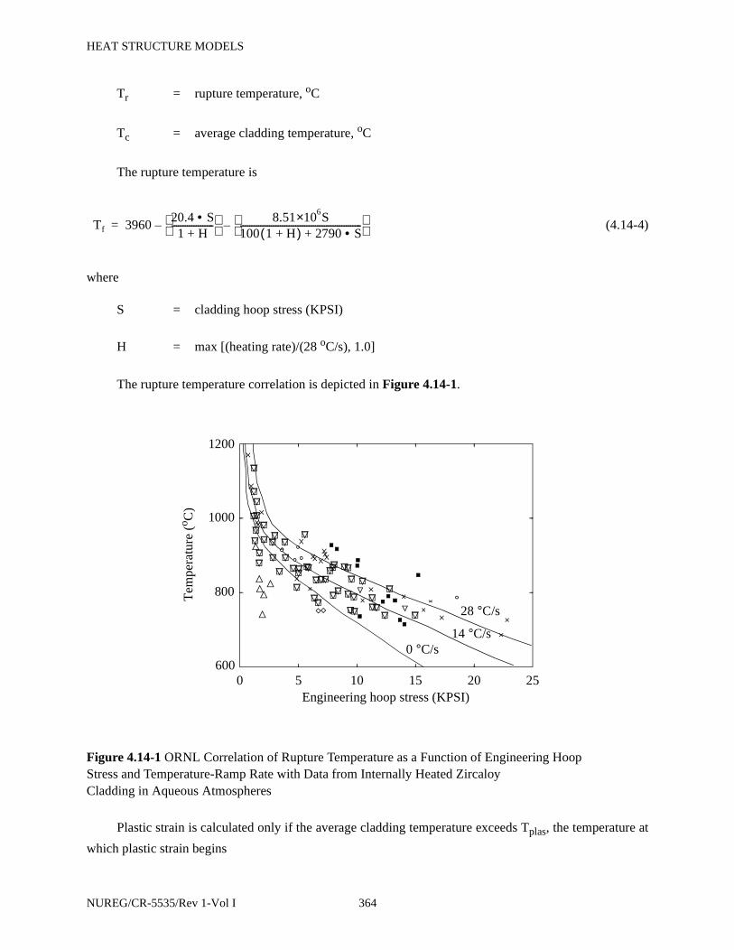
HEAT STRUCTURE MODELS
Tr = rupture temperature, oC
Tc = average cladding temperature, oC
The rupture temperature is
(4.14-4)
where
S = cladding hoop stress (KPSI)
H = max [(heating rate)/(28 oC/s), 1.0]
The rupture temperature correlation is depicted in Figure 4.14-1.
Plastic strain is calculated only if the average cladding temperature exceeds Tplas, the temperature at
which plastic strain begins
Figure 4.14-1 ORNL Correlation of Rupture Temperature as a Function of Engineering Hoop Stress and Temperature-Ramp Rate with Data from Internally Heated Zircaloy Cladding in Aqueous Atmospheres
Tf 396020.4 S•1 H+
------------------- –
8.51 6×10 S100 1 H+( ) 2790 S•+-------------------------------------------------------
–=
0 5 10 15 20 25Engineering hoop stress (KPSI)
600
800
1000
1200
Tem
pera
ture
(o C
)
0 °C/s14 °C/s
28 °C/s
NUREG/CR-5535/Rev 1-Vol I 364

HEAT STRUCTURE MODELS
(4.14-5)
If the average cladding temperature exceeds the value of Tplas, then the rupture temperature is
used together with the heating rate to determine the rupture strain Erup, via a table lookup. When rupture
occurs, a similar table lookup is used to obtain the flow blockage. The rupture strain and blockage tables
are from Reference 4.14-2. The correlations used for cladding strain and rupture are given in Table 4.14-1
and illustrated in Figure 4.14-2 through Figure 4.14-4.
Table 4.14-1 Tabulation of Cladding Correlations
Slow-ramp correlations(< 10 °C/s)
Fast-ramp correlations(< 25 °C/s)
Rupture temperature
(°C)
Burst strain(%)
Flow blockage(%)
Burst strain(%)
Flow blockage (%)
600 10 6.5 10 6.5
625 11 7.0 10 6.5
650 13 8.4 12 7.5
675 20 13.8 15 10.0
700 45 33.5 20 13.8
725 67 52.5 28 20.0
750 82 65.8 38 27.5
775 89 71.0 48 35.7
800 90 71.5 57 43.3
825 89 71.0 60 46.0
850 82 65.8 60 46.0
875 67 52.5 57 43.3
900 48 35.7 45 33.5
925 28 20.0 28 20.0
Tplas Tf 70–= Tf 700<Tplas Tf 70– 0.14 Tf 700–( )–= 700 Tf 1300< <
Tplas Tf 155–= 1300 Tf<
365 NUREG/CR-5535/Rev 1-Vol I
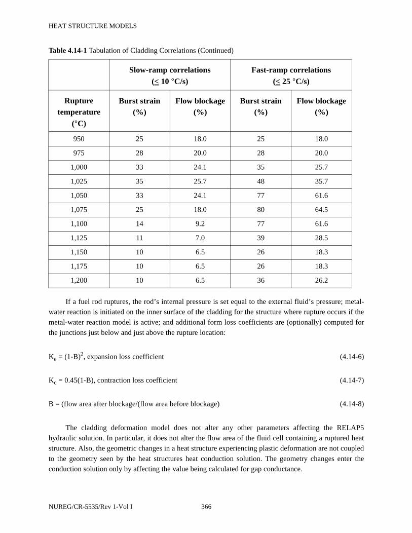
HEAT STRUCTURE MODELS
If a fuel rod ruptures, the rod’s internal pressure is set equal to the external fluid’s pressure; metal-
water reaction is initiated on the inner surface of the cladding for the structure where rupture occurs if the
metal-water reaction model is active; and additional form loss coefficients are (optionally) computed for
the junctions just below and just above the rupture location:
Ke = (1-B)2, expansion loss coefficient (4.14-6)
Kc = 0.45(1-B), contraction loss coefficient (4.14-7)
B = (flow area after blockage/(flow area before blockage) (4.14-8)
The cladding deformation model does not alter any other parameters affecting the RELAP5
hydraulic solution. In particular, it does not alter the flow area of the fluid cell containing a ruptured heat
structure. Also, the geometric changes in a heat structure experiencing plastic deformation are not coupled
to the geometry seen by the heat structures heat conduction solution. The geometry changes enter the
conduction solution only by affecting the value being calculated for gap conductance.
950 25 18.0 25 18.0
975 28 20.0 28 20.0
1,000 33 24.1 35 25.7
1,025 35 25.7 48 35.7
1,050 33 24.1 77 61.6
1,075 25 18.0 80 64.5
1,100 14 9.2 77 61.6
1,125 11 7.0 39 28.5
1,150 10 6.5 26 18.3
1,175 10 6.5 26 18.3
1,200 10 6.5 36 26.2
Table 4.14-1 Tabulation of Cladding Correlations (Continued)
Slow-ramp correlations(< 10 °C/s)
Fast-ramp correlations(< 25 °C/s)
Rupture temperature
(°C)
Burst strain(%)
Flow blockage(%)
Burst strain(%)
Flow blockage (%)
NUREG/CR-5535/Rev 1-Vol I 366

HEAT STRUCTURE MODELS
Figure 4.14-2 Maximum Circumferential Strain as a Function of Rupture Temperature for Internally Heated Zircaloy Cladding in Aqueous Atmospheres at Heating Rates Less Than or Equal to 10 C/s
Figure 4.14-3 Maximum Circumferential Strain as a Function of Rupture Temperature for Internally Heated Zircaloy Cladding in Aqueous Atmospheres at Heating Rates Greater Than or Equal to 25 C/s
600 800 1000 1200Temperature (oC)
0
20
40
60
80
100
120
Cir
cum
fere
ntia
l str
ain
(%)
600 800 1000 1200
Temperature (oC)
0
20
40
60
80
100
Cir
cum
fere
ntia
l str
ain
(%)
367 NUREG/CR-5535/Rev 1-Vol I

HEAT STRUCTURE MODELS
When the reflood fine mesh rezoning algorithm is active, the deformation model sees only the coarse
zones. Deformation calculations are not done for each of the fine mesh points in a axial set of heat
structures. Rather, the deformation calculation is done once for each of the axial heat structures and all of
the fine mesh nodes within a particular heat structure having the same gap conductance value.
4.14.1 References
4.14-1. S. C. Resch et al. FRAP-T6: The Transient Fuel Rod Behavior Code. NUREG/CR-2950. IdahoNational Engineering Laboratory. September 1982.
4.14-2. D. A. Powers and R. O. Meyer. Cladding Swelling and Rupture Models for LOCA Analysis.NUREG-0630. April 1980.
Figure 4.14-4 Reduction in PWR Assembly Flow Area as a Function of Rupture Temperature and Ramp
600 800 1000 1200Temperature (oC)
0
20
40
60
80
100
Red
uctio
n in
flo
w a
rea
(%)
slow-rampfast-ramp
NUREG/CR-5535/Rev 1-Vol I 368
TRIP SYSTEM
5 TRIP SYSTEM
The trip system consists of the evaluation of logical statements. Each trip statement is a simple
logical statement that has a true or false result and an associated variable, TIMEOF. The TIMEOF variable
is -1.0 whenever the trip is false, and contains the time the trip was last set true whenever the trip is true.
This variable allows for time delays and unit step functions based on events during the transient.
Within the structure of RELAP5, the trip system is considered to be only the evaluation of the logical
statements. The decision of what action is needed, based on trip status, resides within other models. For
example, valve models are provided that open or close the valve based on trip values; pump models test
trip status to determine whether a pump electrical breaker has tripped.
Two types of trip statements are provided--variable and logical trips. Since logical trips involve
variable trips and other logical trips, complex logical expressions can be constructed from simple logical
statements. Both types of trips can be latched or unlatched. A latched trip, once set true, is no longer tested
and remains true for the remainder of the problem or until reset at a restart. An unlatched trip is evaluated
every time step.
5.1 Variable Trips
A variable trip evaluates the statement
Tri = V1 OP (V2 + C) (5.1-1)
The value Tri is the i-th trip variable that may be true or false. Values V1 and V2 are quantities from
the heat structures, hydrodynamics, reactor kinetics, control systems, or may be a TIMEOF quantity. The
value C is a constant. The operation OP is one of the following arithmetic relational operations: EQ is
equal, NE is not equal, GT is greater than, GE is greater than or equal, LT is less than, and LE is less than
or equal.
Trips are evaluated at the beginning of the overall RELAP5 time advancement and are evaluated in
numerical order. Except for TIMEOF variables, all other V quantities have beginning of time step values;
and the results of the trip evaluation are independent of the evaluation order. But when a variable trip
statement references TIMEOF (Trk), the new value of TIMEOF is used if k < i.
5.2 Logical Trips
A logical trip evaluates
Tri = + Trj OP + Trl (5.2-1)
369 NUREG/CR-5535/Rev 1-Vol I

TRIP SYSTEM
The values Trj and Trl are variable or logical trips, and the minus sign, if present, denotes the
complement of the trip value. The operation OP is one of the logical operations AND, OR (inclusive or), or
XOR (exclusive or).
Logical trips are evaluated following the evaluation of variable trips and are evaluated in numerical
order. When Trj (or Trl) is a variable trip, new trip values are used; when Trj is a logical trip used in logical
trip expression i, new values are used when j < i and old values are used when j > i.
NUREG/CR-5535/Rev 1-Vol I 370

CONTROL SYSTEM
6 CONTROL SYSTEM
The control system provides the capability to evaluate simultaneous algebraic and ordinary
differential equations. The capability is primarily intended to simulate control systems typically used in
hydrodynamic systems, but it can also model other phenomena described by algebraic and ordinary
differential equations (see Section 8.4.5 for a description of special controllers for use in steady-state
initialization). Another use is to define auxiliary output quantities, such as differential pressures, so they
can be printed in major and minor edits and be plotted.
The control system consists of several types of control components. Each component defines a
control variable as a specific function of time-advanced quantities. The time-advanced quantities include
hydrodynamic volume, junction, pump, valve, heat structure, reactor kinetics, trip quantities, and the
control variables themselves (including the control variable being defined). This permits control variables
to be developed from components that perform simple, basic operations.
In the following equations that define the control components and associated numerical techniques,
Yi is the control variable defined by the i-th control component, Aj, R, and S are real constants input by the
user, I is an integer constant input by the user, Vj is a quantity advanced in time by RELAP5 and can
include Yi, t is time, and s is the Laplace transform variable. Superscripts involving the index n denote time
levels. The name in parentheses to the right of the definition is used in input data to specify the component.
6.1 Arithmetic Control Components
6.1.1 Constant
Yi = S (CONSTANT) (6.1-1)
6.1.2 Addition-Subtraction
Y = S (Ao + A1V1 + A2V2 + …) (SUM) (6.1-2)
6.1.3 Multiplication
Yi = S V1 V2 … (MULT) (6.1-3)
6.1.4 Division
Yi = or Yi = (DIV) (6.1-4)S
V1------
SV2
V1----------
371 NUREG/CR-5535/Rev 1-Vol I
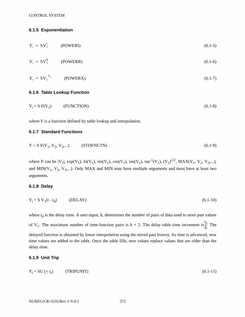
CONTROL SYSTEM
6.1.5 Exponentiation
(POWERI) (6.1-5)
(POWERR) (6.1-6)
(POWERX) (6.1-7)
6.1.6 Table Lookup Function
Yi = S F(V1) (FUNCTION) (6.1-8)
where F is a function defined by table lookup and interpolation.
6.1.7 Standard Functions
Y = S F(V1, V2, V3,...) (STDFNCTN) (6.1-9)
where F can be |V1|, exp(V1), ln(V1), sin(V1), cos(V1), tan(V1), tan-1(V1), (V1)1/2, MAX(V1, V2, V3,...),
and MIN(V1, V2, V3,...). Only MAX and MIN may have multiple arguments and must have at least two
arguments.
6.1.8 Delay
Yi = S V1(t - td) (DELAY) (6.1-10)
where td is the delay time. A user-input, h, determines the number of pairs of data used to store past values
of V1. The maximum number of time-function pairs is h + 2. The delay table time increment is The
delayed function is obtained by linear interpolation using the stored past history. As time is advanced, new
time values are added to the table. Once the table fills, new values replace values that are older than the
delay time.
6.1.9 Unit Trip
Yi = SU (+ tr) (TRIPUNIT) (6.1-11)
Yi SV1I=
Yi SV1R=
Yi SV1V2=
td
h---
NUREG/CR-5535/Rev 1-Vol I 372

CONTROL SYSTEM
6.1.10 Trip Delay
Yi = STr (tr) (TRIPDLAY) (6.1-12)
In the above two trip-related components, tr is a trip number and, if negative (TRIPUNIT only),
indicates that the complement of the trip is to be used; U is 0.0 or 1.0, depending on trip tr (or its
complement if tr is negative) being false or true; and Tr is -1.0 if the trip is false and the time the trip was
last set true if the trip is true.
No numerical approximations are involved in evaluating the algebraic components. Evaluation is by
simply performing the indicated operations. In the sequence of operations that perform a time
advancement of the trip, heat conduction, hydrodynamic, reactor kinetic, and control systems of RELAP5,
the control system is processed last. Thus, the end of time step (n + 1) values for trip variables tr and all V1
variables except control variables Yi are available. The control components are evaluated in component
number order. As the first control variable Y1 is being evaluated, only old-time values are available for all
control component variables. Once Y1 is evaluated, the new-time value for Y1 is available for the
remaining control variable evaluations of Yi. In general, while Yi is being evaluated, new-time values are
available for Yk, k < i, and only old-time values are available for Yk, k > i.
In the example,
(6.1-13)
T and P, which represent a temperature and pressure from the heat structure or hydrodynamic systems, are
new-time values. The value Y8 is also a new-time value because it was advanced before control component
10, and Y10 and Y15 are old-time values.
Initialization of the algebraic control components is very similar to a time advancement. At the start
of control component initialization, all other time-advanced quantities have been initialized. Control
component input includes an initial value and a flag that indicates if initialization is to be performed. The
initialization proceeds in the order of component numbers. The initial value entered becomes the initial
value if no initialization is specified. If initialization is specified, it is simply the specified computation
using the available data. If component i references Yk, k < i, the initialized value of Yk is used; if k > i, the
entered initial value is used.
6.2 Integration Control Component
The integration component evaluates
Y10n 1+ Ao A1Tn 1+ A2Pn 1+ A3Y8
n 1+ A4Y10n A5Y15
n+ + + + +=
373 NUREG/CR-5535/Rev 1-Vol I
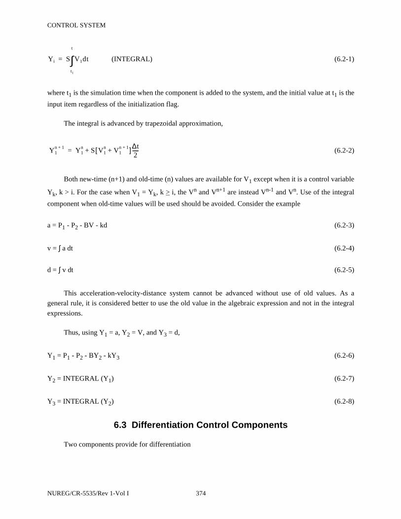
CONTROL SYSTEM
(INTEGRAL) (6.2-1)
where t1 is the simulation time when the component is added to the system, and the initial value at t1 is the
input item regardless of the initialization flag.
The integral is advanced by trapezoidal approximation,
(6.2-2)
Both new-time (n+1) and old-time (n) values are available for V1 except when it is a control variable
Yk, k > i. For the case when V1 = Yk, k > i, the Vn and Vn+1 are instead Vn-1 and Vn. Use of the integral
component when old-time values will be used should be avoided. Consider the example
a = P1 - P2 - BV - kd (6.2-3)
v = ∫ a dt (6.2-4)
d = ∫ v dt (6.2-5)
This acceleration-velocity-distance system cannot be advanced without use of old values. As a
general rule, it is considered better to use the old value in the algebraic expression and not in the integral
expressions.
Thus, using Y1 = a, Y2 = V, and Y3 = d,
Y1 = P1 - P2 - BY2 - kY3 (6.2-6)
Y2 = INTEGRAL (Y1) (6.2-7)
Y3 = INTEGRAL (Y2) (6.2-8)
6.3 Differentiation Control Components
Two components provide for differentiation
Yi S V1dt
t1
t
∫=
Y1n 1+ Y1
n S V1n V1
n 1++[ ] ∆t2-----+=
NUREG/CR-5535/Rev 1-Vol I 374
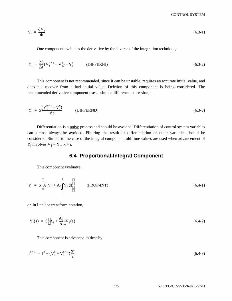
CONTROL SYSTEM
(6.3-1)
One component evaluates the derivative by the inverse of the integration technique,
(DIFFERNI) (6.3-2)
This component is not recommended, since it can be unstable, requires an accurate initial value, and
does not recover from a bad initial value. Deletion of this component is being considered. The
recommended derivative component uses a simple difference expression,
(DIFFERND) (6.3-3)
Differentiation is a noisy process and should be avoided. Differentiation of control system variables
can almost always be avoided. Filtering the result of differentiation of other variables should be
considered. Similar to the case of the integral component, old-time values are used when advancement of
Yi involves V1 = Yk, k > i.
6.4 Proportional-Integral Component
This component evaluates
(PROP-INT) (6.4-1)
or, in Laplace transform notation,
(6.4-2)
This component is advanced in time by
(6.4-3)
Yi
dV1
dt---------=
Yi2S∆t------ V1
n 1+ V1n–( ) Yi
n–=
Yi SV1
n 1+ V1n–( )
∆t-----------------------------=
Yi S A1V1 A2 V1dt
t1
t
∫+
=
Yi s( ) S A1
A2
s------+
V1 s( )=
In 1+ In V1n V1
n 1++( )∆t2-----+=
375 NUREG/CR-5535/Rev 1-Vol I
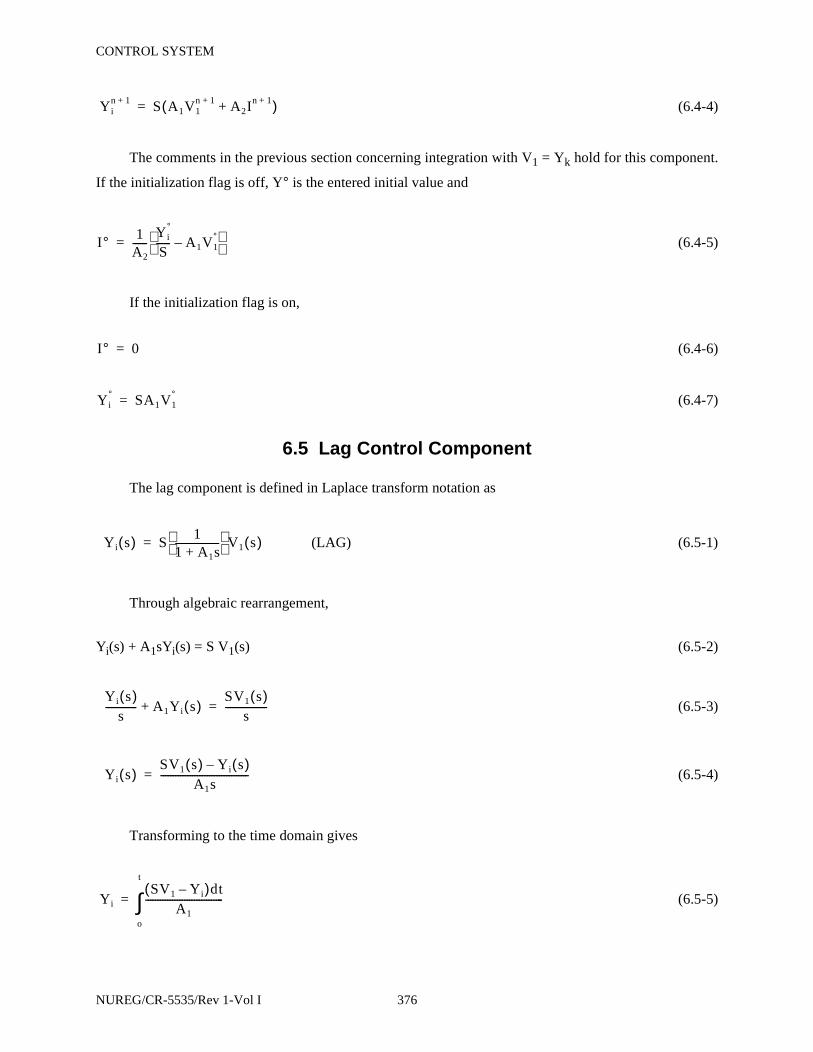
CONTROL SYSTEM
(6.4-4)
The comments in the previous section concerning integration with V1 = Yk hold for this component.
If the initialization flag is off, Y° is the entered initial value and
(6.4-5)
If the initialization flag is on,
(6.4-6)
(6.4-7)
6.5 Lag Control Component
The lag component is defined in Laplace transform notation as
(LAG) (6.5-1)
Through algebraic rearrangement,
Yi(s) + A1sYi(s) = S V1(s) (6.5-2)
(6.5-3)
(6.5-4)
Transforming to the time domain gives
(6.5-5)
Yin 1+ S A1V1
n 1+ A2In 1++( )=
I° 1A2------
Yi°
S------ A1V1
°– =
I° 0=
Yi° SA1V1
°=
Yi s( ) S1
1 A1s+------------------
V1 s( )=
Yi s( )s
------------- A1Yi s( )+SV1 s( )
s-----------------=
Yi s( )SV1 s( ) Yi s( )–
A1s------------------------------------=
Yi
SV1 Yi–( )dtA1
--------------------------------
o
t
∫=
NUREG/CR-5535/Rev 1-Vol I 376

CONTROL SYSTEM
The above expression is advanced numerically by
(6.5-6)
or
(6.5-7)
If the initialization flag is not set, is the entered initial value. If it is set,
(6.5-8)
6.6 Lead-Lag Control Component
The lead-lag component is defined in Laplace transform notation as
(LEAD-LAG) (6.6-1)
Rearranging algebraically, this yields
Yi(s) + A2sYi(s) = SV1(s) + A1s SV1(s) (6.6-2)
or
(6.6-3)
Transforming to the time domain gives
(6.6-4)
Yin 1+ Yi
n S V1n V1
n 1++( ) Yin Yi
n 1+––[ ] ∆t2A1---------+=
Yin 1+
Yin 1
∆t2A1---------–
S V1n V1
n 1++( ) ∆t2A1---------+
1∆t
2A1---------+
----------------------------------------------------------------------------------=
Yi°
Yi° SV1
°=
Yi s( ) S1 A1s+1 A2s+------------------
V1 s( )=
Yi s( )A1SV1 s( )
A2------------------------
SV1 s( ) Yi s( )–A2s
------------------------------------+=
Yi
A1SV1
A2----------------
SV1 Yi–A2
---------------------dt
o
t
∫+=
377 NUREG/CR-5535/Rev 1-Vol I
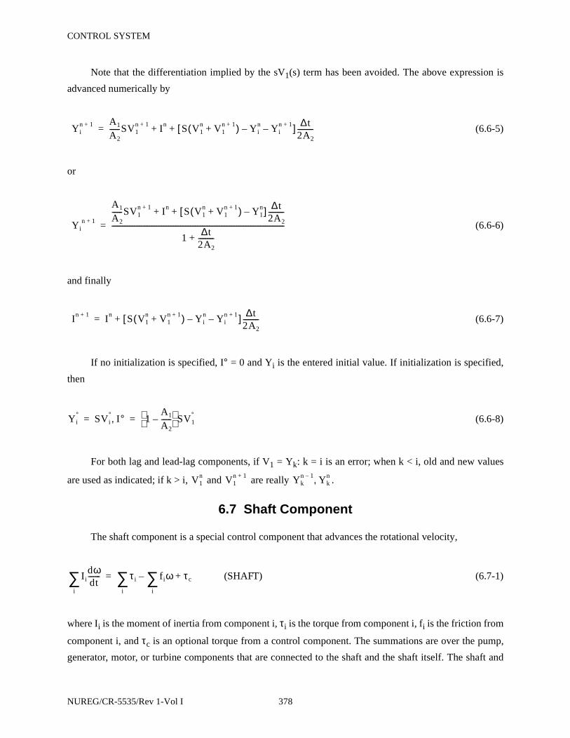
CONTROL SYSTEM
Note that the differentiation implied by the sV1(s) term has been avoided. The above expression is
advanced numerically by
(6.6-5)
or
(6.6-6)
and finally
(6.6-7)
If no initialization is specified, I° = 0 and Yi is the entered initial value. If initialization is specified,
then
(6.6-8)
For both lag and lead-lag components, if V1 = Yk: k = i is an error; when k < i, old and new values
are used as indicated; if k > i, and are really .
6.7 Shaft Component
The shaft component is a special control component that advances the rotational velocity,
(SHAFT) (6.7-1)
where Ii is the moment of inertia from component i, τi is the torque from component i, fi is the friction from
component i, and τc is an optional torque from a control component. The summations are over the pump,
generator, motor, or turbine components that are connected to the shaft and the shaft itself. The shaft and
Yin 1+ A1
A2------SV1
n 1+ In S V1n V1
n 1++( ) Yin– Yi
n 1+–[ ] ∆t2A2---------+ +=
Yin 1+
A1
A2------SV1
n 1+ In S V1n V1
n 1++( ) Y1n–[ ] ∆t
2A2---------+ +
1∆t
2A2---------+
-----------------------------------------------------------------------------------------------------=
In 1+ In S V1n V1
n 1++( ) Yin– Yi
n 1+–[ ] ∆t2A2---------+=
Yi° SVi
° I°, 1A1
A2------–
SV1°= =
V1n V1
n 1+ Ykn 1– Yk
n,
Iidωdt-------
i
∑ τ i fiω τc+i
∑–i
∑=
NUREG/CR-5535/Rev 1-Vol I 378
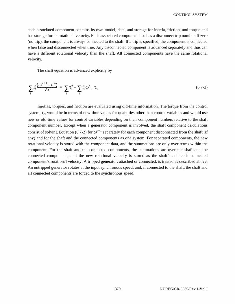
CONTROL SYSTEM
each associated component contains its own model, data, and storage for inertia, friction, and torque and
has storage for its rotational velocity. Each associated component also has a disconnect trip number. If zero
(no trip), the component is always connected to the shaft. If a trip is specified, the component is connected
when false and disconnected when true. Any disconnected component is advanced separately and thus can
have a different rotational velocity than the shaft. All connected components have the same rotational
velocity.
The shaft equation is advanced explicitly by
(6.7-2)
Inertias, torques, and friction are evaluated using old-time information. The torque from the control
system, τc, would be in terms of new-time values for quantities other than control variables and would use
new or old-time values for control variables depending on their component numbers relative to the shaft
component number. Except when a generator component is involved, the shaft component calculations
consist of solving Equation (6.7-2) for ωn+1 separately for each component disconnected from the shaft (if
any) and for the shaft and the connected components as one system. For separated components, the new
rotational velocity is stored with the component data, and the summations are only over terms within the
component. For the shaft and the connected components, the summations are over the shaft and the
connected components; and the new rotational velocity is stored as the shaft’s and each connected
component’s rotational velocity. A tripped generator, attached or connected, is treated as described above.
An untripped generator rotates at the input synchronous speed; and, if connected to the shaft, the shaft and
all connected components are forced to the synchronous speed.
Iin ωn 1+ ωn–( )
∆t-----------------------------
i
∑ τ in fi
nωn τ c+i
∑–i
∑=
379 NUREG/CR-5535/Rev 1-Vol I

CONTROL SYSTEM
NUREG/CR-5535/Rev 1-Vol I 380

POINT REACTOR KINETICS MODEL
7 POINT REACTOR KINETICS MODEL
The point reactor kinetics model can be used to compute power behavior in a nuclear reactor. The
power is computed using the space-independent or point kinetics approximation which assumes that power
can be separated into space and time functions. This approximation is adequate for cases in which the
space distribution remains nearly constant.
The point reactor kinetics model computes both the immediate fission power and the power from
decay of fission products. The immediate power is that released at the time of fission and includes power
from kinetic energy of the fission products and neutron moderation. Decay power is generated as the
fission products undergo radioactive decay. The user can select the decay power model based on either the
American Nuclear Society Proposed Standard ANS 5.1, Decay Energy Release Rates Following Shutdown
of Uranium-Fueled Thermal Reactors, revised October 1973, or the American National Standard for Decay
Heat Power in Light Water Reactors, ANSI/ANS-5.1-1979.
7.1 Point Reactor Kinetics Equations
The point kinetics equations are
(7.1-1)
(7.1-2)
(7.1-3)
Pf(t) = Qfψ(t) (7.1-4)
where
t = time
ϕ = neutron flux
Ci = number of delayed neutron precursors of group
β = effective delayed neutron fraction
Λ = prompt neutron generation time
tdd ϕ t( ) ρ t( ) β–[ ]ϕ t( )
Λ----------------------------------- λ iCi t( )
i 1=
Nd
∑ S+ +=
tdd
Ci t( )βfi
Λ------ϕ t( ) λ iCi t( ) i– 1 2 … Nd, , ,= =
ψ t( ) Σfϕ t( )=
i
381 NUREG/CR-5535/Rev 1-Vol I

POINT REACTOR KINETICS MODEL
ρ = reactivity (only the time-dependence has been indicated; however, thereactivity is dependent on other variables)
fi = fraction of delayed neutrons of group i
λi = decay constant of group i
S = source
ψ = fission rate in #/s
= macroscopic fission cross-section
Pf = immediate fission power in MeV/s
Qf = immediate fission energy per fission in MeV
7.2 Fission Product Decay Model
The 1979 standard expresses the power Psα (t) in MeV/s as a function of time t resulting from one
fission of isotope α at t = 0 as
(7.2-1)
Data are presented for three isotopes, 235U, 238U, and 239Pu. The parameters a and λ were obtained
by fitting to fission decay power data. The fitting for each isotope used 23 groups (Nα = 23). The above
expression is an impulse response to one fission and can be extended to an arbitrary fission rate ψα(t)
through the convolution integral
(7.2-2)
where the convolution operation is defined by
(7.2-3)
Σf
Psα t( ) aα jexp λα jt–( )j 1=
Nα
∑=
Pα t( ) Psα t( )*ψα t( ) aα jexp λα jt–( )*ψα t( )j 1=
Nα
∑= =
A t( )*B t( ) A t τ–( )0
t
∫ B τ( ) τd A τ( )B t τ–( ) τd0
t
∫= =
NUREG/CR-5535/Rev 1-Vol I 382

POINT REACTOR KINETICS MODEL
Since numerical evaluation of convolution integrals is cumbersome, a set of differential equations
equivalent to the convolution integral is derived.
Assume that the power from each group is from radioactive decay of a fission fragment i. Then
Pαj (t) = λαjγαj (t) = aαjexp(-λαjt) (7.2-4)
For simplification in the following derivation, the α and j subscripts are dropped and the following
expressions represent an equation for one group for one isotope. From Equation (7.2-4) we have
(7.2-5)
Laplace transforming Equation (7.2-5) gives
(7.2-6)
Rearranging Equation (7.2-6) gives
(7.2-7)
Transforming to real time yields
(7.2-8)
where δ(0) is the impulse function. Applying a time-dependent fission rate ψ(t) in place of the single
fission (impulse response), Equation (7.2-7) and (7.2-8) become
(7.2-9)
(7.2-10)
γ t( ) aλ---exp λ t–( )=
γ s( ) aλ s λ+( )--------------------=
sγ s( ) aλ--- λγ s( )–=
tdd γ t( ) a
λ---δ 0( ) λγ t( )–=
sγ s( ) aλ---ψ s( )= λγ s( )–
tdd γ t( ) a
λ---ψ t( ) λγ t( )–=
383 NUREG/CR-5535/Rev 1-Vol I
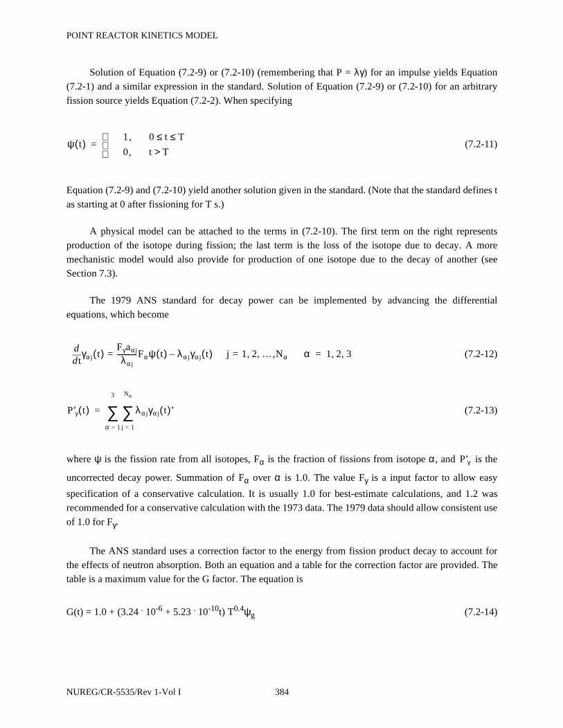
POINT REACTOR KINETICS MODEL
Solution of Equation (7.2-9) or (7.2-10) (remembering that P = λγ) for an impulse yields Equation
(7.2-1) and a similar expression in the standard. Solution of Equation (7.2-9) or (7.2-10) for an arbitrary
fission source yields Equation (7.2-2). When specifying
(7.2-11)
Equation (7.2-9) and (7.2-10) yield another solution given in the standard. (Note that the standard defines t
as starting at 0 after fissioning for T s.)
A physical model can be attached to the terms in (7.2-10). The first term on the right represents
production of the isotope during fission; the last term is the loss of the isotope due to decay. A more
mechanistic model would also provide for production of one isotope due to the decay of another (see
Section 7.3).
The 1979 ANS standard for decay power can be implemented by advancing the differential
equations, which become
(7.2-12)
(7.2-13)
where ψ is the fission rate from all isotopes, Fα is the fraction of fissions from isotope α, and is the
uncorrected decay power. Summation of Fα over α is 1.0. The value Fγ is a input factor to allow easy
specification of a conservative calculation. It is usually 1.0 for best-estimate calculations, and 1.2 was
recommended for a conservative calculation with the 1973 data. The 1979 data should allow consistent use
of 1.0 for Fγ.
The ANS standard uses a correction factor to the energy from fission product decay to account for
the effects of neutron absorption. Both an equation and a table for the correction factor are provided. The
table is a maximum value for the G factor. The equation is
G(t) = 1.0 + (3.24 . 10-6 + 5.23 . 10-10t) T0.4ψg (7.2-14)
ψ t( ) 1, 0 t T≤ ≤
0, t T>
=
tdd γα j t( )
Fγaα j
λα j------------Fαψ t( ) λα jγα j t( ) j– 1 2 …, ,= = ,Nα α 1 2 3, ,=
P’γ t( ) λα jγα j t( )j 1=
Nα
∑ ’
α 1=
3
∑=
P’γ
NUREG/CR-5535/Rev 1-Vol I 384

POINT REACTOR KINETICS MODEL
where ψg is the number of fissions per initial fissile atom, T is the reactor operating time including any
periods of shutdown, and t is the time since shutdown. Limits on the quantities are 1.0 > ψg > 3.0, T <
1.2614 . 108 seconds, and t < 104 seconds. The table is used for t > 104. Note that there is a discontinuity in
G(t) when switching from the equation to the table. The standard allows the table to be used in place of the
equation and the code through user input allows the same. The corrected decay power is given by
(7.2-15)
The 1973 proposed standard uses one isotope and prescribes data for 11 groups. The 1979 standard
lists data for three isotopes, 235U, 238U, and 239Pu, and uses 23 groups for each isotope. A user option also
allows only the 1979 standard data for 235U to be used. The data for both standards are built into the code
as default data, but the user may enter different data.
7.3 Actinide Decay Model
The actinide model describes the production of 239U, 239Np, and 239Pu from neutron capture by238U.
(7.3-1)
(7.3-2)
(7.3-3)
The quantity FU is user-specified and is the number of atoms of 239U produced by neutron capture in
238U per fission from all isotopes. A conservative factor if desired should be factored into FU. The λ and ηvalues can be user-specified, or default values equal to those stated in the 1979 ANS standard can be used.
The first equation describes the rate of change of atoms of 239U. The first term on the right represents
the production of 239U; the last term is the loss of 239U due to beta decay. The second equation describes
the rate of change of 239Np. The production of 239Np is from the beta decay of 239U, and 239Pu is formed
from the decay of 239Np. Solution of the actinide Equations, Equation (7.3-1) and (7.3-2), for the fission
source given in Equation (7.2-11) yields the result quoted in the 1979 standard.
Pγ G t( )P’γ=
tdd γU t( ) FUψ t( ) λUγU t( )–=
tdd γN t( ) λUγU t( ) λNγN t( )–=
Pα t( ) ηUλUγU t( ) ηNλNγN t( )+=
385 NUREG/CR-5535/Rev 1-Vol I

POINT REACTOR KINETICS MODEL
7.4 Transformation of Equations for Solution
The differential equations to be advanced in time are Equation (7.1-1), (7.1-2), (7.2-12), (7.3-1), and
(7.3-2). Multiplying by and X which is the conversion factor from MeV/s to watts, the equations
become
(7.4-1)
(7.4-2)
(7.4-3)
(7.4-4)
(7.4-5)
The total power PT is the sum of immediate fission power, corrected fission product decay, and
actinide decay, and now in units of watts is
(7.4-6)
For solution convenience, the following substitutions are made:
ρ (t) = βr (t) (7.4-7)
(7.4-8)
(7.4-9)
Σf
tdd
Xψ t( )[ ] ρ t( ) β–[ ] Xψ t( )Λ
---------------------------------------- λ iXΣfCi t( )i 1=
Nd
∑ XΣfS+ +=
tdd
XΣfCi t( )[ ]βfiXψ t( )
Λ---------------------- λ iXΣfCi t( )–=
tdd
Xγα j t( )[ ]Fγaα jFαXψ t( )
λα j---------------------------------- λα jXγα j t( )–=
tdd
XγU t( )[ ] FUXψ t( ) λUXγU t( )–=
tdd
XγN t( )[ ] λ UXγU t( ) λNXγN t( )–=
PT t( ) QfXψ t( ) G t( ) λα jXγα j t( )j 1=
Nα
∑α 1=
3
∑ ηUλUXγU t( ) ηNλNXγN t( )+ + +=
Xψ t( ) ψ’ t( )=
XΣfΛSβ
----------------- S’=
NUREG/CR-5535/Rev 1-Vol I 386
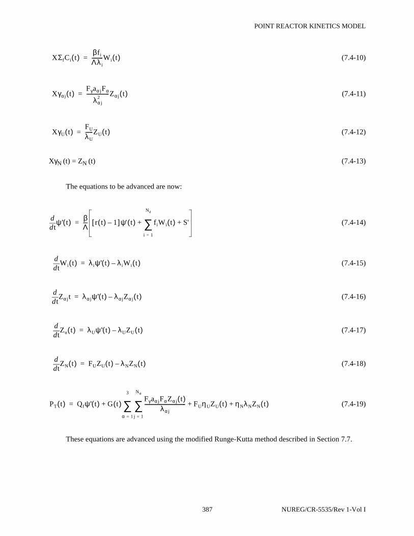
POINT REACTOR KINETICS MODEL
(7.4-10)
(7.4-11)
(7.4-12)
XγN (t) = ZN (t) (7.4-13)
The equations to be advanced are now:
(7.4-14)
(7.4-15)
(7.4-16)
(7.4-17)
(7.4-18)
(7.4-19)
These equations are advanced using the modified Runge-Kutta method described in Section 7.7.
XΣfCi t( )βfi
Λλ i---------Wi t( )=
Xγα j t( )Fγaα jFα
λα j2
------------------Zα j t( )=
XγU t( )FU
λU------ZU t( )=
tdd ψ’ t( ) β
Λ---- r t( ) 1–[ ]ψ ' t( ) fiWi t( )
i 1=
Nd
∑ S'+ +=
tdd
Wi t( ) λ iψ’ t( ) λ iWi t( )–=
tdd
Zα jt λα jψ’ t( ) λα jZα j t( )–=
tdd
Zu t( ) λUψ’ t( ) λUZU t( )–=
tdd
ZN t( ) FUZU t( ) λNZN t( )–=
PT t( ) Qfψ’ t( ) G t( )Fγaα jFαZα j t( )
λα j---------------------------------
j 1=
Nα
∑α 1=
3
∑ FUηUZU t( ) ηNλNZN t( )+ + +=
387 NUREG/CR-5535/Rev 1-Vol I

POINT REACTOR KINETICS MODEL
7.5 Initialization
Two initialization options are provided. In both options, the fission rate and delayed neutrons are in
steady-state or equilibrium conditions, that is, their time derivatives are zero. With r(0) an input quantity,
(7.5-1)
(7.5-2)
The first option assumes that the fission product decay and actinides are also in equilibrium. This is
equivalent to assuming that the reactor has been operating at a constant total power for an infinite period of
time. The initial conditions are
(7.5-3)
(7.5-4)
(7.5-5)
(7.5-6)
(7.5-7)
The quantity Q, which is the total energy in MeV generated per fission, is either an input value or can
be defaulted to 200 MeV. The quantity Qf is defined from Equation (7.5-7) and the user-specified or
defaulted data, even if the second initialization option is used. The total power is an input quantity, and
is determined from Equation (7.5-6). The remaining quantities are computed from using
Equation (7.5-1) through (7.5-5). Depending on a user option, the G factor is evaluated from Equation
(7.2-14) with the reactor operating time T set to the user input and the operating time t set to zero or from
the first value in the G factor table in the standard (1.020).
The second option uses a power history to determine the initial values of the fission product and
actinide quantities. The power history consists of one or more periods of constant total power. For each
Wi 0( ) ψ’ 0( ) i 1 2 … Nd, , ,= =
S’ r 0( )ψ’ 0( )–=
Zα j 0( ) ψ’ 0( ) i=1,2,...,Nα α 1 2 3, ,= =
ZU 0( ) ψ’ 0( )=
ZN 0( )FU
λN------ψ’ 0( )=
PT 0( ) Qf G 0( )Fγaα jFα
λα j------------------Zα j 0( )
j 1=
Nα
∑α 1=
3
∑ FUηUZU 0( ) ηNλNZN 0( )+ + + ψ’ 0( )=
Q Qf Fγaα jFα
j 1=
Nα
∑α 1=
3
∑ FUηU FUηN+ + +=
ψ’ 0( ) ψ’ 0( )
NUREG/CR-5535/Rev 1-Vol I 388
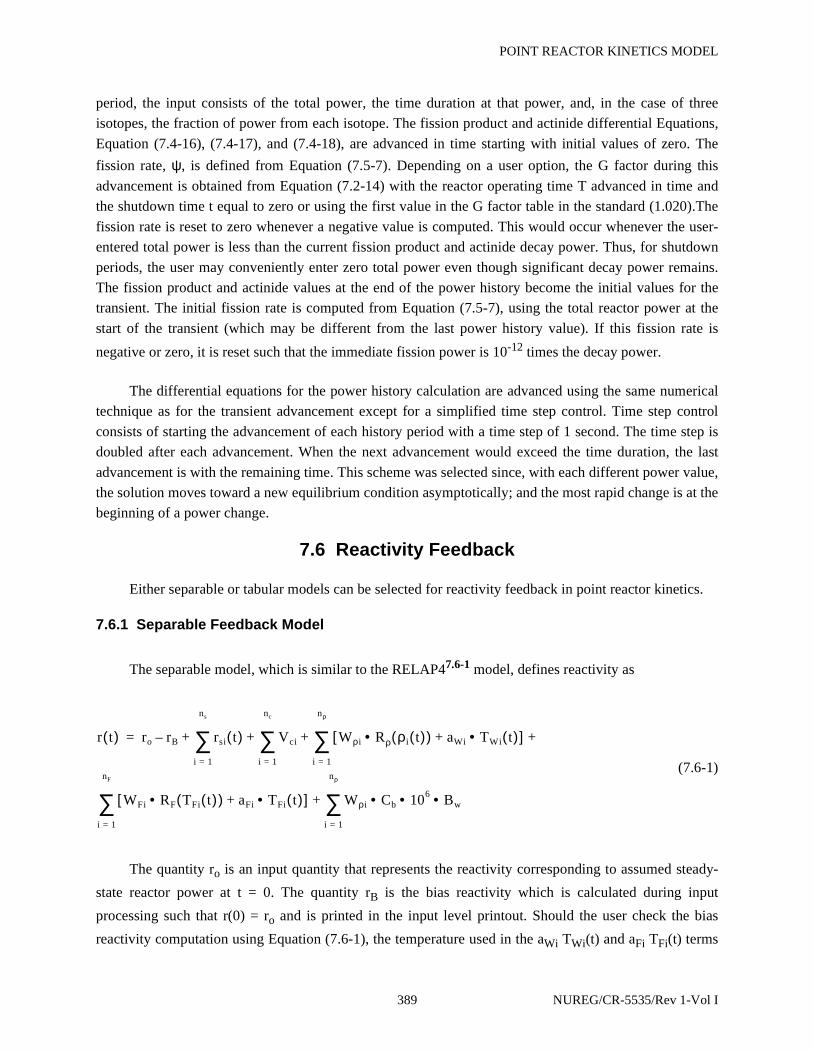
POINT REACTOR KINETICS MODEL
period, the input consists of the total power, the time duration at that power, and, in the case of three
isotopes, the fraction of power from each isotope. The fission product and actinide differential Equations,
Equation (7.4-16), (7.4-17), and (7.4-18), are advanced in time starting with initial values of zero. The
fission rate, ψ, is defined from Equation (7.5-7). Depending on a user option, the G factor during this
advancement is obtained from Equation (7.2-14) with the reactor operating time T advanced in time and
the shutdown time t equal to zero or using the first value in the G factor table in the standard (1.020).The
fission rate is reset to zero whenever a negative value is computed. This would occur whenever the user-
entered total power is less than the current fission product and actinide decay power. Thus, for shutdown
periods, the user may conveniently enter zero total power even though significant decay power remains.
The fission product and actinide values at the end of the power history become the initial values for the
transient. The initial fission rate is computed from Equation (7.5-7), using the total reactor power at the
start of the transient (which may be different from the last power history value). If this fission rate is
negative or zero, it is reset such that the immediate fission power is 10-12 times the decay power.
The differential equations for the power history calculation are advanced using the same numerical
technique as for the transient advancement except for a simplified time step control. Time step control
consists of starting the advancement of each history period with a time step of 1 second. The time step is
doubled after each advancement. When the next advancement would exceed the time duration, the last
advancement is with the remaining time. This scheme was selected since, with each different power value,
the solution moves toward a new equilibrium condition asymptotically; and the most rapid change is at the
beginning of a power change.
7.6 Reactivity Feedback
Either separable or tabular models can be selected for reactivity feedback in point reactor kinetics.
7.6.1 Separable Feedback Model
The separable model, which is similar to the RELAP47.6-1 model, defines reactivity as
(7.6-1)
The quantity ro is an input quantity that represents the reactivity corresponding to assumed steady-
state reactor power at t = 0. The quantity rB is the bias reactivity which is calculated during input
processing such that r(0) = ro and is printed in the input level printout. Should the user check the bias
reactivity computation using Equation (7.6-1), the temperature used in the aWi TWi(t) and aFi TFi(t) terms
r t( ) ro rB– rsi t( )i 1=
ns
∑ Vci
i 1=
nc
∑ Wρi R• ρ ρi t( )( ) aWi TWi• t( )+[ ]i 1=
nρ
∑+ + + +=
WFi RF• TFi t( )( ) aFi TFi• t( )+[ ] Wρi Cb 106 Bw•••i 1=
nρ
∑+
i 1=
nF
∑
389 NUREG/CR-5535/Rev 1-Vol I
POINT REACTOR KINETICS MODEL
should use absolute temperature, i.e., Kelvin in SI units and Rankine in British units. The temperature used
in the table lookup term WFi RF[TFi(t)], however, should still use Kelvin in SI units and Fahrenheit in
British units.
The quantities rsi are obtained from input tables defining ns reactivity curves as a function of time.
The quantities Vci are nc control variables that can be user-defined as reactivity contributions. Rρ is a table
defining reactivity as a function of the current density of water ρi(t) in the hydrodynamic volume i; Wρi is
the density weighting factor for volume i; TWi(t) is the spatial density averaged temperature of volume i;
aWi is the temperature coefficient (not including density changes) for volume i; and nρ is the number of
hydrodynamic volumes in the reactor core. The quantity RF is a table defining reactivity as a function of
the volume average fuel temperature TFi(t) in heat structure i; WFi and aFi are the fuel temperature
weighting factor and the fuel temperature coefficient, respectively; and nF is the number of heat structures
in the reactor core. The quantity is the boron concentration in mass of boron per mass of
liquid water and BW is the differential boron worth in $/ppm. This quantity is normally found in core
design reports as pcm/ppm and must be converted to $/ppm. The units, pcm, are per cent mille or 10-5 of
∆k/k, while dollars are measured in units of the delayed neutron fraction, ∆k/(kβ).
The model assumes nonlinear feedback effects from moderator density and fuel temperature changes
and linear feedback from moderator temperature changes. It is called the separable model because each
effect is assumed to be independent of the other effects. The separable model can be used if boron changes
are quite small and the reactor is near critical about only one state point.
7.6.2 Tabular Feedback Model
A postulated BWR anticipated transient without scram (ATWS) accident is an example where the
reactor could be nearly critical for two different state points. One point is at normal power operating
conditions--high moderator and fuel temperatures, highly voided, and no boron. During accident recovery,
the reactor might approach a critical condition with relatively cold moderator and fuel temperatures, with
no voids, but with some boron concentration. The reactivity could be nearly critical for both states, but the
contributions from the different feedback effects are vastly different. The assumptions of no interactions
among the different feedback mechanisms, especially boron, cannot be justified.
The tabular feedback model computes reactivity from multi-dimensional table lookup and linear
interpolation. The tabular model overcomes the objections of the separable model since all feedback
mechanisms can be nonlinear and interactions among the mechanisms are included. The penalty for the
expanded modeling capability is greatly increased input data requirements.
Two different sets of variables within the tabular feedback option are available. Both sets of variables
allow a boron related variable as one of the four variables. Both sets of variables allow the boron related
variable to be omitted when only three variables are used.
Cb ρb α fρf( )⁄=
NUREG/CR-5535/Rev 1-Vol I 390
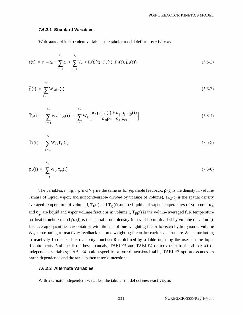
POINT REACTOR KINETICS MODEL
7.6.2.1 Standard Variables.
With standard independent variables, the tabular model defines reactivity as
(7.6-2)
(7.6-3)
(7.6-4)
(7.6-5)
(7.6-6)
The variables, ro, rB, rsi, and Vci are the same as for separable feedback, ρi(t) is the density in volume
i (mass of liquid, vapor, and noncondensable divided by volume of volume), TWi(t) is the spatial density
averaged temperature of volume i, Tfi(t) and Tgi(t) are the liquid and vapor temperatures of volume i, αfi
and αgi are liquid and vapor volume fractions in volume i, TFi(t) is the volume averaged fuel temperature
for heat structure i, and ρbi(t) is the spatial boron density (mass of boron divided by volume of volume).
The average quantities are obtained with the use of one weighting factor for each hydrodynamic volume
Wρi contributing to reactivity feedback and one weighting factor for each heat structure WFi contributing
to reactivity feedback. The reactivity function R is defined by a table input by the user. In the Input
Requirements, Volume II of these manuals, TABLE3 and TABLE4 options refer to the above set of
independent variables; TABLE4 option specifies a four-dimensional table, TABLE3 option assumes no
boron dependence and the table is then three-dimensional.
7.6.2.2 Alternate Variables.
With alternate independent variables, the tabular model defines reactivity as
r t( ) ro rB– rsi
i 1=
ns
∑ Vci
i 1=
nc
∑ R ρ t( ) Tw t( ) TF t( ) ρb t( ),,,( )+ + +=
ρ t( ) Wρiρi t( )i 1=
nρ
∑=
Tw t( ) WρiTWi t( )i 1=
nρ
∑ Wρi
α fiρfiTfi t( ) αgiρgiTgi t( )+α fiρfi αgiρgi+
--------------------------------------------------------------
i 1=
nρ
∑= =
TF t( ) WFiTFi t( )i 1=
nF
∑=
ρb t( ) Wρiρbi t( )i 1=
nρ
∑=
391 NUREG/CR-5535/Rev 1-Vol I
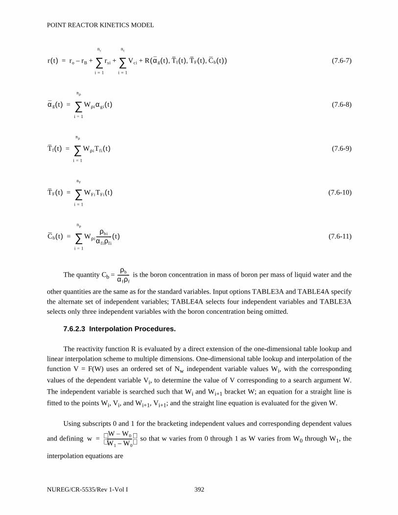
POINT REACTOR KINETICS MODEL
(7.6-7)
(7.6-8)
(7.6-9)
(7.6-10)
(7.6-11)
The quantity Cb = is the boron concentration in mass of boron per mass of liquid water and the
other quantities are the same as for the standard variables. Input options TABLE3A and TABLE4A specify
the alternate set of independent variables; TABLE4A selects four independent variables and TABLE3A
selects only three independent variables with the boron concentration being omitted.
7.6.2.3 Interpolation Procedures.
The reactivity function R is evaluated by a direct extension of the one-dimensional table lookup and
linear interpolation scheme to multiple dimensions. One-dimensional table lookup and interpolation of the
function V = F(W) uses an ordered set of Nw independent variable values Wi, with the corresponding
values of the dependent variable Vi, to determine the value of V corresponding to a search argument W.
The independent variable is searched such that Wi and Wi+1 bracket W; an equation for a straight line is
fitted to the points Wi, Vi, and Wi+1, Vi+1; and the straight line equation is evaluated for the given W.
Using subscripts 0 and 1 for the bracketing independent values and corresponding dependent values
and defining so that w varies from 0 through 1 as W varies from W0 through W1, the
interpolation equations are
r t( ) ro rB– rsi
i 1=
nc
∑ Vci
i 1=
nc
∑ R αg t( ) Tf t( ) TF t( ) Cb t( ),,,( )+ + +=
α g t( ) Wρiαgi t( )i 1=
nρ
∑=
Tf t( ) WρiTfi t( )i 1=
nρ
∑=
TF t( ) WFiTFi t( )i 1=
nF
∑=
Cb t( ) Wρi
ρbi
α fiρfi------------- t( )
i 1=
nρ
∑=
ρb
α fρf----------
wW W0–W1 W0–---------------------
=
NUREG/CR-5535/Rev 1-Vol I 392
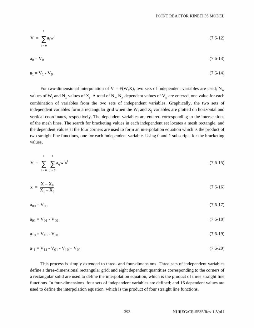
POINT REACTOR KINETICS MODEL
(7.6-12)
a0 = V0 (7.6-13)
a1 = V1 - V0 (7.6-14)
For two-dimensional interpolation of V = F(W,X), two sets of independent variables are used; Nw
values of Wi and Nx values of Xj. A total of Nw Nx dependent values of Vij are entered, one value for each
combination of variables from the two sets of independent variables. Graphically, the two sets of
independent variables form a rectangular grid when the Wi and Xj variables are plotted on horizontal and
vertical coordinates, respectively. The dependent variables are entered corresponding to the intersections
of the mesh lines. The search for bracketing values in each independent set locates a mesh rectangle, and
the dependent values at the four corners are used to form an interpolation equation which is the product of
two straight line functions, one for each independent variable. Using 0 and 1 subscripts for the bracketing
values,
(7.6-15)
(7.6-16)
a00 = V00 (7.6-17)
a01 = V01 - V00 (7.6-18)
a10 = V10 - V00 (7.6-19)
a11 = V11 - V01 - V10 + V00 (7.6-20)
This process is simply extended to three- and four-dimensions. Three sets of independent variables
define a three-dimensional rectangular grid; and eight dependent quantities corresponding to the corners of
a rectangular solid are used to define the interpolation equation, which is the product of three straight line
functions. In four-dimensions, four sets of independent variables are defined; and 16 dependent values are
used to define the interpolation equation, which is the product of four straight line functions.
V aiwi
i 0=
1
∑=
V aijwixj
j 0=
1
∑i 0=
1
∑=
xX X0–X1 X0–------------------=
393 NUREG/CR-5535/Rev 1-Vol I
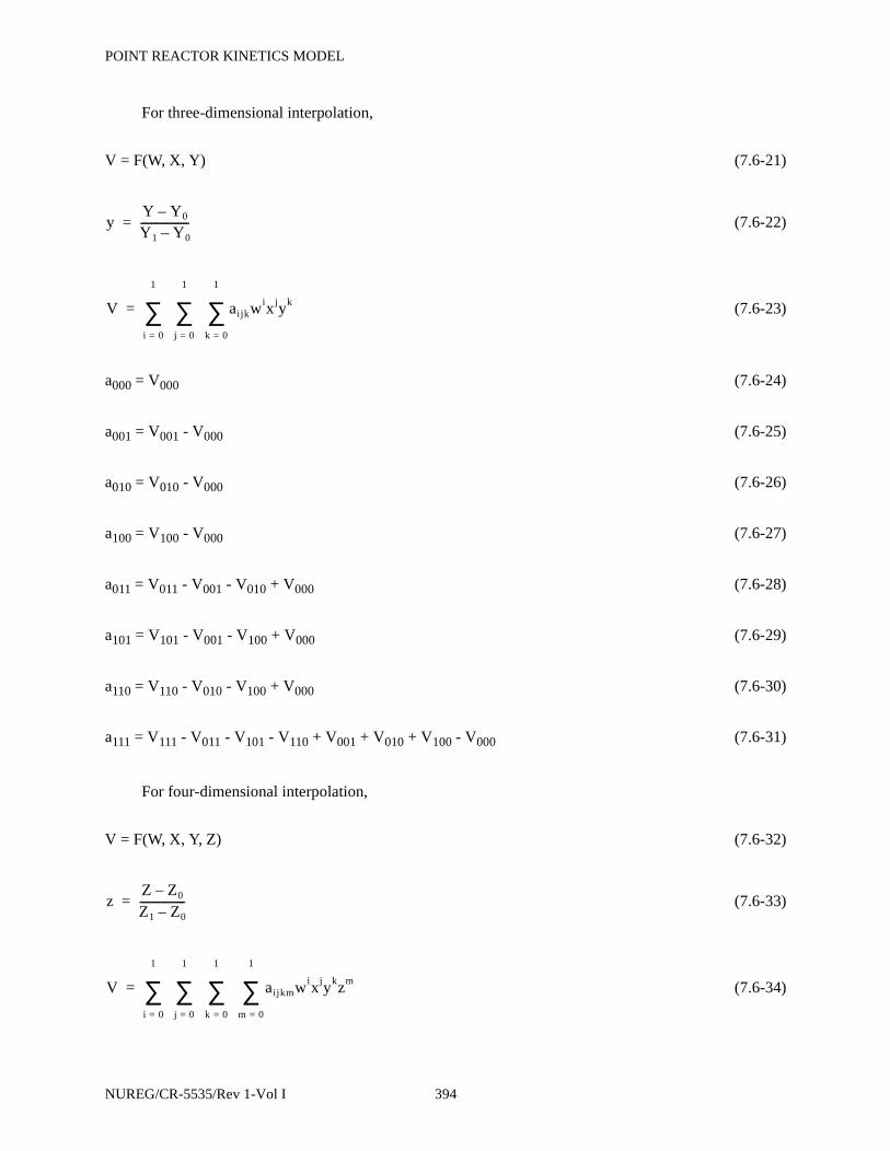
POINT REACTOR KINETICS MODEL
For three-dimensional interpolation,
V = F(W, X, Y) (7.6-21)
(7.6-22)
(7.6-23)
a000 = V000 (7.6-24)
a001 = V001 - V000 (7.6-25)
a010 = V010 - V000 (7.6-26)
a100 = V100 - V000 (7.6-27)
a011 = V011 - V001 - V010 + V000 (7.6-28)
a101 = V101 - V001 - V100 + V000 (7.6-29)
a110 = V110 - V010 - V100 + V000 (7.6-30)
a111 = V111 - V011 - V101 - V110 + V001 + V010 + V100 - V000 (7.6-31)
For four-dimensional interpolation,
V = F(W, X, Y, Z) (7.6-32)
(7.6-33)
(7.6-34)
yY Y0–Y1 Y0–------------------=
V aijkwixjyk
k 0=
1
∑j 0=
1
∑i 0=
1
∑=
zZ Z0–Z1 Z0–-----------------=
V aijkmwixjykzm
m 0=
1
∑k 0=
1
∑j 0=
1
∑i 0=
1
∑=
NUREG/CR-5535/Rev 1-Vol I 394

POINT REACTOR KINETICS MODEL
a0000 = V0000 (7.6-35)
a0001 = V0001 - V0000 (7.6-36)
a0010 = V0010 - V0000 (7.6-37)
a0100 = V0100 - V0000 (7.6-38)
a1000 = V1000 - V0000 (7.6-39)
a0011 = V0011 - V0001 - V0010 + V0000 (7.6-40)
a0101 = V0101 - V0001 - V0100 + V0000 (7.6-41)
a0110 = V0110 - V0010 - V0100 + V0000 (7.6-42)
a1001 = V1001 - V0001 - V1000 + V0000 (7.6-43)
a1010 = V1010 - V0010 - V1000 + V0000 (7.6-44)
a1100 = V1100 - V0100 - V1000 + V0000 (7.6-45)
a0111 = V0111 - V0011 - V0101 + V0110 + V0001 + V0010 + V0100 - V0000 (7.6-46)
a1011 = V1011 - V0011 - V1001 + V1010 + V0001 + V0010 + V1000 - V0000 (7.6-47)
a1101 = V1101 - V0101 - V1001 + V1100 + V0001 + V0100 + V1000 - V0000 (7.6-48)
a1110 = V1110 - V0110 - V1010 + V1100 + V0010 + V0100 + V1000 - V0000 (7.6-49)
a1111 = V1111 - V0111 - V1011 - V1101 - V1110 + V0011 + V0101 + V0110 + V1101 +V1001 +V1010 + V1100 - V0001 - V0010 - V0100 - V1000 + V0000 . (7.6-50)
The interpolating equations define a continuous function. There is no discontinuity in the dependent
quantity as any one or combination of dependent variables pass to the next bracketing pair of values.
395 NUREG/CR-5535/Rev 1-Vol I
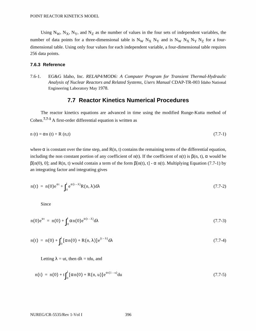
POINT REACTOR KINETICS MODEL
Using NW, NX, NY, and NZ as the number of values in the four sets of independent variables, the
number of data points for a three-dimensional table is NW NX NY and is NW NX NY NZ for a four-
dimensional table. Using only four values for each independent variable, a four-dimensional table requires
256 data points.
7.6.3 Reference
7.6-1. EG&G Idaho, Inc. RELAP4/MOD6: A Computer Program for Transient Thermal-HydraulicAnalysis of Nuclear Reactors and Related Systems, Users Manual CDAP-TR-003 Idaho National
Engineering Laboratory May 1978.
7.7 Reactor Kinetics Numerical Procedures
The reactor kinetics equations are advanced in time using the modified Runge-Kutta method of
Cohen.7.7-1 A first-order differential equation is written as
n (t) = αn (t) + R (n,t) (7.7-1)
where α is constant over the time step, and R(n, t) contains the remaining terms of the differential equation,
including the non constant portion of any coefficient of n(t). If the coefficient of n(t) is β(n, t), α would be
β[n(0), 0]; and R(n, t) would contain a term of the form β[n(t), t] - α n(t). Multiplying Equation (7.7-1) by
an integrating factor and integrating gives
(7.7-2)
Since
(7.7-3)
(7.7-4)
Letting λ = ut, then dλ = tdu, and
(7.7-5)
n t( ) n 0( )eα t eα t λ–( )R n λ,( ) λd0
t
∫+=
n 0( )eα t n 0( ) αn 0( )eα t λ–( ) λd0
t
∫+=
n t( ) n 0( ) αn 0( ) R n λ,( )+[ ] e t λ–( ) λd0
t
∫+=
n t( ) n 0( ) t αn 0( ) R n u,( )+[ ] eα t 1 u–( ) ud0
1
∫+=
NUREG/CR-5535/Rev 1-Vol I 396
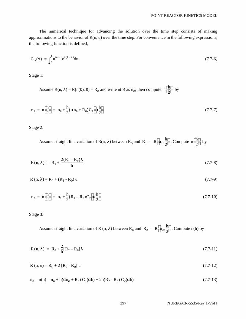
POINT REACTOR KINETICS MODEL
The numerical technique for advancing the solution over the time step consists of making
approximations to the behavior of R(n, u) over the time step. For convenience in the following expressions,
the following function is defined,
(7.7-6)
Stage 1:
Assume R(n, λ) = R[n(0), 0] = Ro and write n(o) as no; then compute by
(7.7-7)
Stage 2:
Assume straight line variation of R(n, λ) between Ro and . Compute by
(7.7-8)
R (n, λ) = R0 + (R1 - R0) u (7.7-9)
(7.7-10)
Stage 3:
Assume straight line variation of R (n, λ) between Ro and . Compute n(h) by
(7.7-11)
R (n, u) = R0 + 2 [R2 - R0] u (7.7-12)
n3 = n(h) = no + h(αno + Ro) C1(αh) + 2h(R2 - Ro) C2(αh) (7.7-13)
Cm x( ) um 1– ex 1 u–( ) ud0
1
∫=
nh2---
n1 nh2---
n0h2--- αn0 R0+( )C1 α h
2---
+= =
R1 R n1h2---,
= nh2---
R n λ,( ) R0
2 R1 R0–( )λh
------------------------------+=
n2 nh2---
n1h2--- R1 R0–( )C2 α h
2---
+= =
R2 R n2h2---,
=
R n λ,( ) R02h--- R2 R0–[ ]λ+=
397 NUREG/CR-5535/Rev 1-Vol I

POINT REACTOR KINETICS MODEL
Stage 4:
Assume quadratic through points Ro, R2, and R3 = R(n3, h), then compute n(h) by
R(n, u) = (2Ro + 4R2 + 2R3) u2 + (-3Ro + 4R2 - R3) u + Ro (7.7-14)
n4 = n(h) = n3 + h (R4 - R3) [2C3 (αh) - C2(αh)] (7.7-15)
Stage 5:
Assume quadratic through points Ro, R2, and R4 = R(n4, h), then compute n(h) by
n5 = n(h) = n4 + h (R4 - R3) [2C3 (αh) - C2 (αh)] . (7.7-16)
Third-, fourth-, and fifth-order approximations are obtained by terminating the process at the end of
the third-, fourth-, and fifth-stages, respectively. RELAP5 uses only the fifth-order approximation.
By direct integration, the function C1(x) is given by
(7.7-17)
Using integration by parts, a recursion relation for Cm(x) is
(7.7-18)
During machine calculations of the Cm(x) functions for x < 1, excessive loss of significance occurs.
For this range, C3(x) is computed from its MacLaurin series expansion
(7.7-19)
C2 and C1 are evaluated by solving Equation (7.7-18) for Cm (x).
During the advancement in time of the solution, the time increment is automatically increased or
decreased to maintain a specified degree of accuracy. After the calculations for a reactor kinetics time
advancement, an empirical formula is used to estimate the error. If the error is excessive, the time
C1 x( ) ex 1–x
-------------=
Cm 1+ x( )mCm x( ) 1–
x-----------------------------=
C3 x( ) 213!-----
x4!-----
x2
5!-----
x3
6!-----
x4
7!-----
x5
8!-----
x6
9!-----
x7
10!--------+ + + + + + +
=
NUREG/CR-5535/Rev 1-Vol I 398
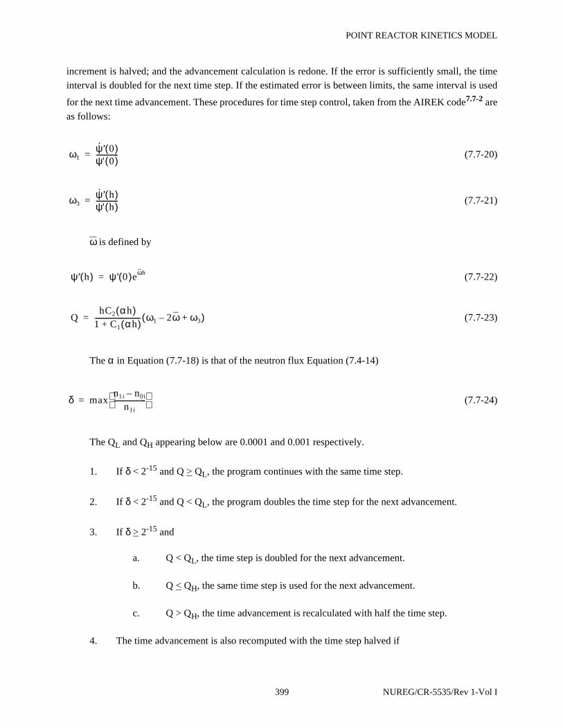
POINT REACTOR KINETICS MODEL
increment is halved; and the advancement calculation is redone. If the error is sufficiently small, the time
interval is doubled for the next time step. If the estimated error is between limits, the same interval is used
for the next time advancement. These procedures for time step control, taken from the AIREK code7.7-2 are
as follows:
(7.7-20)
(7.7-21)
ω is defined by
(7.7-22)
(7.7-23)
The α in Equation (7.7-18) is that of the neutron flux Equation (7.4-14)
(7.7-24)
The QL and QH appearing below are 0.0001 and 0.001 respectively.
1. If δ < 2-15 and Q > QL, the program continues with the same time step.
2. If δ < 2-15 and Q < QL, the program doubles the time step for the next advancement.
3. If δ > 2-15 and
a. Q < QL, the time step is doubled for the next advancement.
b. Q < QH, the same time step is used for the next advancement.
c. Q > QH, the time advancement is recalculated with half the time step.
4. The time advancement is also recomputed with the time step halved if
ω1ψ’· 0( )ψ' 0( )-------------=
ω3ψ’· h( )ψ' h( )-------------=
ψ’ h( ) ψ’ 0( )eωh=
QhC2 αh( )
1 C1 αh( )+--------------------------- ω1 2ω– ω3+( )=
δ maxn1i n0i–
n1i-------------------
=
399 NUREG/CR-5535/Rev 1-Vol I

POINT REACTOR KINETICS MODEL
a. αh of any equation > 88
b. negative or zero power is computed
If the coefficient of the neutron flux in Equation (7.4-14) is negative, a subtraction is involved in
determination of the derivative and a loss of significant digits can occur. If this coefficient is negative, a
check is made of the number of bits lost in the subtraction. If more than nine bits are lost, the value of
neutron flux computed by the current stage of the advancement procedure is discarded; instead, neutron
flux is determined from the expression obtained by setting the neutron flux derivative to zero
(7.7-25)
The transfer of information between the reactor kinetics calculation and the other calculations is
explicit. Hydrodynamic and heat conduction/transfer calculation precede reactor kinetics, and the control
system calculation follows reactor kinetics. The reactor power used in hydrodynamics and heat conduction
is the value at the beginning of the time step. The reactivity used as the end of time step value in the
kinetics advancement is computed from end of time step values from hydrodynamics and heat conduction
and beginning of time step values from the control system.
The reactor kinetics equations are advanced at the same time step as the hydrodynamics, and
reactivity is assumed to vary linearly between time step values. The maximum time step for the reactor
kinetics advancement is the hydrodynamic time step. That time step is reduced, if necessary, as described
above.
7.7.1 References
7.7-1. E. R. Cohen “Some Topics In Reactor Kinetics” A/CONF 15 1958 p. 629.
7.7-2. A. Schwartz Generalized Reactor Kinetics Code AIREK II NAA-SR-Memo-4980 1960.
ψ t( )
fiWi t( )i 1=
Nd
∑–SΛβ
-------–
r t( ) 1–--------------------------------------------=
NUREG/CR-5535/Rev 1-Vol I 400

SPECIAL TECHNIQUES
8 SPECIAL TECHNIQUES
The mass from the state relationship is compared to the mass from the continuity equation, and the
difference is a measure of the truncation error inherent in the numerical solution. This is the main method
used to control the time step and thus control the truncation error. Other methods are also used.
Special techniques are also used to mitigate mass and energy errors. These are (1) a second
evaluation of the semi-implicit scheme equations using non-linearized time derivatives, (2) velocity flip-
flop situations, and (3) noncondensable gas appearance situations.
Special methods are provided in the code for use in obtaining initial conditions. These methods are
based on the transient solution algorithm but make use of an accelerated thermal transient solution
technique in order to shorten the computer time required to achieve steady-state. Generic control
component options are available to allow the user to minimize the time, effort, and cost to achieve steady-
state.
8.1 Time Step Control
A variety of checks on solution acceptability are used to control the time step. These include Courant
limit checks, mass error checks, material properties out of defined ranges, water property errors, excessive
extrapolation of state properties in the metastable regimes, phase appearance/disappearance checks, or
large pressure changes in a volume when a noncondensable gas appears.
The Courant limit check is made before a hydrodynamic advancement takes place. Thus, it may
reduce the time step, but it does not cause a time step to be repeated. All of the other checks may cause all
or part of the time advancement to be repeated at a smaller time step.
8.1.1 New Mass/Energy Cell-Based (Material) Courant Limit
The Courant limit is a stability condition that is necessary when explicit, or old-time velocities are
used in the finite-difference form of the momentum equations. Simply stated, this condition for a 1-D finite
control volume is
(8.1-1)
or
(8.1-2)
where
v∆t ∆x≤
∆t∆xv
-------≤
401 NUREG/CR-5535/Rev 1-Vol I
SPECIAL TECHNIQUES
= time step size (s)
= control volume length (m)
v = velocity of flow in the control volume (m/s)
Typically, is a fixed quantity and is determined by the nodalization scheme. In general, a finer
nodalization scheme will result in a more restrictive Courant limit than a coarse scheme. Thus, for a cell of
fixed length, the application of Equation (8.1-2) determines the maximum time step size that can be used to
solve the momentum equations and still guarantee stability,
(8.1-3)
Referring to Figure 8.1-1, since RELAP5 solves for velocity at the junctions which are at the edges
of continuity cells, the following method is used to determine the Courant limit,
(8.1-4)
where
VK,L = volume of upstream volume, volume K or volume L (m3)
Aj = area of junction j (m2)
vj = velocity at junction j (m/s)
When a junction is defined in a RELAP5 deck, a “from” volume and a “to” volume must be
specified. By convention, the “from” volume is called volume K and the “to” volume is called volume L.
When fluid is moving from volume K to volume L, the velocity is positive. When moving from volume L
to volume K, the velocity is negative. During a transient, the upstream volume is determined by inspecting
the sign of the velocity. In the figure, the upstream volume is volume K.
The use of volumes and areas in Equation (8.1-4), instead of cell length, is necessary to account for
geometries and modeling situations other than straight, constant-area pieces of pipe. A separate Courant
limit is calculated at each junction for liquid, and for vapor, since, strictly speaking, the
theory used to derive the limit is only appropriate for single-phase flow. For volumes to which multiple
junctions are attached, the limits corresponding to each junction are summed together to give an overall
estimate of the Courant limit for the cell. The calculations are performed at the beginning of a time step
∆t
∆x
∆x
∆tc∆xv
-------=
∆tc
VK L,
Ajvj-----------=
tc∆( )fj
tc∆( )gj
NUREG/CR-5535/Rev 1-Vol I 402
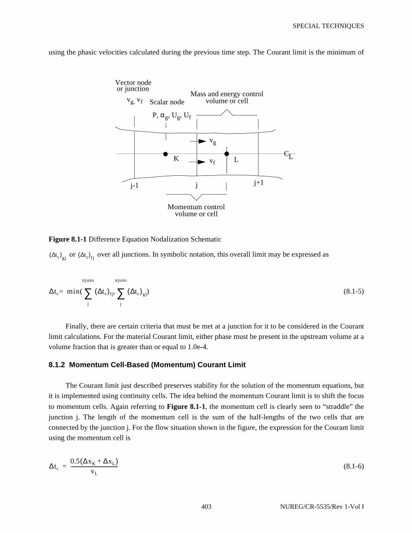
SPECIAL TECHNIQUES
using the phasic velocities calculated during the previous time step. The Courant limit is the minimum of
or over all junctions. In symbolic notation, this overall limit may be expressed as
(8.1-5)
Finally, there are certain criteria that must be met at a junction for it to be considered in the Courant
limit calculations. For the material Courant limit, either phase must be present in the upstream volume at a
volume fraction that is greater than or equal to 1.0e-4.
8.1.2 Momentum Cell-Based (Momentum) Courant Limit
The Courant limit just described preserves stability for the solution of the momentum equations, but
it is implemented using continuity cells. The idea behind the momentum Courant limit is to shift the focus
to momentum cells. Again referring to Figure 8.1-1, the momentum cell is clearly seen to “straddle” the
junction j. The length of the momentum cell is the sum of the half-lengths of the two cells that are
connected by the junction j. For the flow situation shown in the figure, the expression for the Courant limit
using the momentum cell is
(8.1-6)
Figure 8.1-1 Difference Equation Nodalization Schematic
Vector node or junction
vg, vf
j-1
K
Mass and energy controlvolume or cell
vg
vf L
j+1
Scalar node
P, αg, Ug, Uf
Momentum controlvolume or cell
j
CL
tc∆( )gj
tc∆( )fj
∆tc min tc∆( )fj
j
njuns
∑ tc∆( )gj
j
njuns
∑( , )=
∆tc
0.5 ∆xK ∆xL+( )vL
--------------------------------------=
403 NUREG/CR-5535/Rev 1-Vol I

SPECIAL TECHNIQUES
where
= length of volume K (m)
= length of volume L (m)
vL = volume-averaged velocity for volume L (m/s)
The length of the momentum cell is used in the momentum Courant limit calculation instead of using
volumes and areas because it is not always possible to calculate a momentum cell volume and area, such as
for complicated geometries like branches that may have several junctions attached to them. The
momentum cell length is calculated as the average of the lengths of volume K and volume L. The
velocities used to calculate the momentum Courant limit are the continuity cell-centered, or volume
averaged velocities. These velocities are defined at the edges of momentum cells and may be used to
determine the amount of momentum entering/leaving a momentum cell. Only those flows that are leaving
the momentum cell are of interest in the momentum Courant limit calculation. When momentum is being
fluxed out of both faces of the momentum cell (vK<0 and vL>0), the convention will be to only consider
the larger of the two volume-averaged velocities and to calculate a Courant limit using only that larger
term.
As with the old Courant limit, Equation (8.1-6) is calculated for each junction and for each phase;
however, with the momentum cell approach, the contributions from junctions attached to the same volume
are considered separately and are not be summed together.
Courant limit calculations are performed in the subroutine COURN1. Both the material and
momentum Courant limit calculations are performed and the minimum of these two limits is taken as the
overall Courant limit to ensure conservatism. It is this overall Courant limit that is returned to DTSTEP
and used to limit the hydrodynamic time step.
The criteria that must be met at a junction for it to be considered in the momentum Courant limit
calculations are the following conditions for the liquid contribution,
(8.1-7)
and for the vapor contribution,
(8.1-8)
∆xK
∆xL
α fjρfjvfj2
α fjρfjvfj2 αgjρgjvgj
2+----------------------------------------------- 10 10–≥
α gjρgjvgj2
α fjρfjvfj2 αgjρgjvgj
2+----------------------------------------------- 10 10–≥
NUREG/CR-5535/Rev 1-Vol I 404

SPECIAL TECHNIQUES
The denominator is simply the total momentum flux at a junction. Equation (8.1-7) is the fraction of
momentum represented by the liquid phase, and Equation (8.1-8) is the fraction of momentum represented
by the vapor phase at a junction. The limit of 10-10 is rather arbitrary and only effectively serves to prevent
the consideration of a phase in the momentum Courant limit calculation that is not physically present, i.e.
( ).
In COURN1, the reciprocal of the Courant limit is the quantity that is actually calculated, to prevent
a divide by zero calculation if the junction velocity or volume-averaged velocity is ever equal to zero. The
maximum value of this reciprocal value over all the junctions is determined, which is divided into 1.0 after
falling out of the loop. When the momentum Courant limit is more conservative than the material Courant
limit, a lowercase “f” or “g” will be printed to the screen for liquid or vapor, respectively, whereas the
original uppercase “F” or “G” will is printed when the material Courant limit is more conservative.
8.1.3 Original Material Courant Limit
The original material Courant limit is evaluated for each hydrodynamic volume using the phasic
volume velocities and the phasic volume fractions, and it is given by
i = 1, 2,..., N (8.1-9)
The N volumes are divided into five subsets, i.e., the 1st, 6th, 11th,... volumes belong to the first subset, the
2nd, 7th, 12th,... volumes belong to the second subset, etc. The minimum Courant limits for each of the
five subsets are rearranged in ascending order, i.e.,
(8.1-10)
Thus, is the Courant limit for the entire system. This is the number printed at each major edit under
“CRNT. DT =”. For the semi-implicit scheme, is used for limiting the time step size. Thus, partial
violation of the material Courant limit is allowed for this scheme. For the nearly-implicit scheme, 20 times
is used for limiting the time step size for the transient mode, and 40 times is used for limiting the
time step size for the steady-state mode.
8.1.4 Mass Error Check
The mass error check is made when the time step solution is nearly complete. If excessive mass error
is detected, the time step is repeated at a reduced interval. Two types of mass error measures are computed.
The first one is designed to check the validity of the density linearization and is defined as
α f g,( )j 10 8–<
∆tc( )i ∆xi max α fi
n α gin,( )
max α fin vfi
n αgin vgi
n,( )----------------------------------------------------=
∆tc1 ∆tc
2 ∆tc3 ∆tc
4 ∆tc5≤≤≤≤
∆tc1
∆tc2
∆tc2 ∆tc
2
405 NUREG/CR-5535/Rev 1-Vol I

SPECIAL TECHNIQUES
i = 1, 2,..., N (8.1-11)
where ρmi is the total density of the i-th volume obtained from the mass continuity equation, and ρi is the
total density of the i-th volume computed from the state relationship. The second one is a measure of
overall system mass error and is given by
(8.1-12)
If either εm or εrms is > 8 x 10⁻³, the time step is rejected and repeated with one half of the time step
size. Otherwise, the time step is accepted, and the next time step size is doubled if both εm and εrms are
< 8 x 10⁻⁴. The maximum of εm or εrms for all volumes is shown in the major edits Time Step Summary
(ERR.EST) and minor edits/plots (ERRMAX). The value of εm for each system is shown in the individual
system major edits (ERR.EST).
The first type of mass error measure [(ρmi - ρi)Vi] is added for each volume at each time step. This is
the same as computing the mass flowing in through junctions connected to time-dependent volumes,
subtracting the mass flowing out through junctions connected to time-dependent volumes, and adding the
difference between the previous time step mass and the current mass. This mass error is accumulated for
each system and is shown in the system major edits (MASS ERROR) and minor edits/plots (SYSMER).
This mass error is accumulated for all the systems and is shown in the Time Step Summary (MS.ERR) and
minor edits/plots (EMASS). The total mass in each system is shown in the system major edits (MASS) and
minor edits/plots (SYSTMS). The total mass for all systems is shown in the Time Step Summary
(TOT.MS) and minor edits/plots (TMASS). At any given time, the following equation holds:
εm max ρmi ρi–
ρi---------------------
=
εrms
2 Vi ρi ρmi–( )[ ] 2
i 1=
N
∑
Viρi( )2
i 1=
N
∑-----------------------------------------------=
NUREG/CR-5535/Rev 1-Vol I 406

SPECIAL TECHNIQUES
. (8.1-13)
8.1.5 Other Checks
At any point in the solution flow, if a material property is found to lie outside the defined range, the
time step is halved and repeated. This halving process proceeds until the property is within range or the
user-specified minimum time step is reached. If the minimum time step is reached without obtaining a
valid solution, the code calculation is terminated; the last time step is repeated with a diagnostic dump
printed, and the program stops at the completion of the advancement. This same procedure is applied for
all water property or extrapolation failures. The liquid metastable checks used are specific volume less
than or equal to 0 and liquid temperature greater than 50 K above saturation temperature. The vapor
metastable checks are vapor specific volume less than or equal to 0 and the vapor temperature less than
50 K below saturation temperature. The vapor 50 K limit is used for the steam only case, but not for the
noncondensable/steam case which uses iteration. There is also time step control based on problems with
void fraction (αg), noncondensable quality (Xn), and mixture density from the phasic continuity equations
(ρm). Advancements that result in αg and Xn being slightly less than 0.0 or slightly greater than 1.0 are
allowed, and the variable is reset to 0.0 or 1.0. Advancements that result in values much less than 0.0 or
much greater than 1.0 are considered an error, and the time step is repeated. The cutoff points are based on
a functional relationship. This relation is tied to the mass error upper limit (8 x 10⁻³). Advancements that
result in ρm being < 0 are also considered an error and the time step is repeated. In addition, if too much of
one-phase appears (more than a typical thermal boundary layer thickness) starting from a single phase
state, an error is assumed to have occurred, and the time step is repeated. In addition, there is a time step
control based on the change in the pressure in a volume during an advancement, which is used whenever
noncondensable gas first appears in a volume. This time step control algorithm causes the code to repeat a
time step if the change in pressure during a time step exceeds the old-time value, the new-time value, or
50,000 Pa. This time step control has the effect of allowing the pressure to change by no more than a factor
of two during a time step.
mass at
start of
calculation
+ mass flowing in
through junctions
connected to
time dependent
volumes
– mass flowing out
through junctions
connected to
time dependent
volumes
= mass at
current
+ cumulative
mass error
time at current
TMASS( ) time
EMASS( )
407 NUREG/CR-5535/Rev 1-Vol I

SPECIAL TECHNIQUES
Two other checks are done on the change in the void fraction and the vapor internal energy in one
time step. It the absolute change in the void fraction is greater than 0.15, the time step is repeated with the
time step size cut in half. If the absolute relative change in the vapor internal energy is greater than 0.10,
the time step size is cut in half and the time step is repeated.
8.2 Mass/Energy Error Mitigation
The semi-implicit numerical scheme described in Section 3.1.3 and Section 3.1.4 has two
calculations of the new-time variables αg, Ug, Uf, and Xn. These variables are first calculated in connection
with a linearization of all the product terms involved in the time derivatives and are referred to as tentative
new-time variables [see Equation (3.1-87) through (3.1-91)]. They are denoted by a tilde in Section 3.1.3
and Section 3.1.4. This first calculation uses a numerically conservative form for all flux calculations of
mass and energy, but because the products in the time derivatives are linearized, the quantities αgρg, αfρf,
αgρgUg, αfρfUf, and αgρgXn are not numerically conserved. These tentative new-time values are only used
to evaluate the interphase heat and mass transfer terms to be used in the second evaluation of the basic
equations. In this second evaluation of the basic equations [see Equation (3.1-107), (3.1-109), (3.1-110),
(3.1-112), and (3.1-113)], the products appearing in the time derivatives are not linearized. This second
step also uses the numerically conservative form for the flux terms. Hence, the final end of time step values
have been calculated using a consistent and numerically conservative form of differencing. The truncation
errors in the linearization procedure may produce errors in the solution for pressure, phasic energies, and
void fraction. Since the state is computed from these basic variables, the resultant density may have some
error. This error is used in the time step control presented in Section 8.1.
There are mass and energy errors that the numerically conservative form of differencing cannot
remove. The convective terms in the field equations are computed with donored properties determined by
the direction of phasic velocities. There are times that the final velocities may differ in directions from the
explicit velocities used to define the donored properties. This may result in mass/energy errors due to
incorrect properties used in the numerical scheme. The term velocity flip-flop refers to the situation in
which the final velocities and the explicit velocities differ in sign. In the RELAP5 numerical scheme, the
pressures and final velocities are calculated using the donor properties based on the explicit velocities (see
Section 3.1.3). The velocity flip-flop implies that inconsistent donor properties were used for the pressure
computation and the final mass/energy computation. This may result in bad velocity and energy solutions
and large mass errors. Thus, a mitigation scheme is employed to detect errors of this type. Let αfj, ρfj, Ufj,
αgj, ρgj, and Ugj be the junction liquid fraction, liquid density, liquid energy, void fraction, vapor density,
and vapor energy, respectively, based on the explicit velocities, and let and be the
same variables based on the final velocities. A velocity flip-flop has occurred when one of the junctions in
a system satisfies the following condition:
(8.2-1)
α fj ρfj Ufj αgj ρgj, , , , Ugj
α fjρfjUfj αgj+ ρgjUgj α fjρfjUfj α gj– ρgjUgj 0.20 α fjρfjUfj αgj+ ρgjUgj( )>–
NUREG/CR-5535/Rev 1-Vol I 408

SPECIAL TECHNIQUES
Under such circumstances, the pressures and final velocities are recalculated using the donor properties of
the previously calculated final velocities.
Another situation that may cause excessive mass and/or energy errors is when a noncondensable gas
first appears in a volume. Because the linearized phasic properties are evaluated at the state existing at the
beginning of an advancement, the derivatives of the phasic properties with respect to the noncondensable
gas quality will be zero since there is no noncondensable gas in the volume at the beginning of the
advancement. The convection of noncondensable gas into the volume during the advancement will result
in an inconsistent state at the end of the advancement because the derivatives needed for the computation
of a consistent state are identically zero. The inconsistency may be manifested as a large mass error where
the noncondensable gas fails to appear in the volume even though the flux of noncondensable gas into the
volume is positive. The inconsistency may also be manifested as a unphysically high vapor temperature
when noncondensable gas first appears in a volume. This inconsistency is corrected by repeating the
advancement when noncondensable gas first appears in a volume. The code checks for this situation at the
end of every advancement if the noncondensable gas model has been activated by the user. The situation is
detected whenever the noncondensable quality in a volume is zero at the beginning of the advancement and
the flux of noncondensable gas into the volume during the advancement is greater than a small
noncondensable source term. This term (can be zero) was determined from tests of thought problems,
separate effects calculations, integral effects calculations, and plant calculations. The noncondensable
quality and vapor fraction that would result from the flux of noncondensable gas into the volume is
estimated from an explicit mass balance on the vapor phase in the volume. The estimated noncondensable
gas quality is then used in the computation of the derivatives of the phasic properties. The estimated
noncondensable gas quality and vapor fraction are also used in the construction of the linearized
conservation equations instead of the beginning of advancement quantities. The modified linearized
conservation equations are then used to compute the end of advancement quantities as described
previously. The time step size used for the repeated advancement is the same as that used for the original
attempted advancement unless the pressure change in the cell is too large. The time step control based on
the change in the pressure described in Section 8.1 is activated for volumes in which noncondensable gas is
first appearing. The time step control based on pressure may result in multiple time step repeats with
smaller and smaller time steps when a noncondensable gas first appears in a volume.
8.3 Steady-State
A steady-state initialization capability is included in RELAP5. With this capability, the transient
solution algorithm is continually monitored to determine the achievement of a steady-state. During this
process, convergence criteria are calculated and used in the steady-state testing scheme. These
convergence criteria are related to an overall calculational precision. This overall precision is the result of
combining both the precision of the transient solution algorithm and the standard tolerance of the
thermodynamic state algorithm. The following discussion describes the fundamental concepts of tests to
detect steady-state during transient calculations.
8.3.1 Fundamental Concepts for Detecting Hydrodynamic
409 NUREG/CR-5535/Rev 1-Vol I

SPECIAL TECHNIQUES
Steady-State During Transient Calculations
The fundamental concept of steady-state is that the state of a reactor system being modeled does not
change with respect to time. In the hydrodynamic solution scheme, three terms can be monitored whose
variation in time include the variation of all of the other terms. These three terms are the thermodynamic
density, internal energy, and pressure. Furthermore, these three terms can be combined into a single-term,
enthalpy. Hence, monitoring the time variation of enthalpy is equivalent to monitoring the time variation of
all of the other variables in the solution scheme. For each volume cell in the system model, the enthalpy
can be written as
(8.3-1)
where subscript i denotes the i-th volume element, hi is the volume element specific enthalpy in units of
energy per unit mass, and Vi is the element volume. Since volume is constant, Equation (8.3-1) can be
simplified as
(8.3−2)
The rate of variation with respect to time of Equation (8.3-2) can be expressed numerically as
(8.3-3)
Absolute hydrodynamic steady-state occurs when Equation (8.3-3) is zero for each of the volume
elements in the modeled system.
In order to simplify the task of detecting steady-state, a system mean enthalpy can be expressed as
(8.3-4)
A system mean rate of change can also be formulated as
Viρinhi
n Vi ρinUi
n Pin+( )=
ρinhi
n ρinUi
n Pin+=
d ρh( )dt
--------------
i
n ρin 1+ Ui
n 1+ Pin 1++( ) ρi
nUin Pi
n+( )–
∆tn---------------------------------------------------------------------------------=
ρh( )n
Vi ρinUi
n Pin+( )
i 1=
NVOLS
∑
Vi
i 1=
NVOLS
∑-------------------------------------------------=
NUREG/CR-5535/Rev 1-Vol I 410

SPECIAL TECHNIQUES
(8.3-5)
However, since the rate of change in any volume element can be positive or negative, these terms
would tend to cancel. Hence, a better formulation for the mean rate of change is a mean square summation
that can be written as
(8.3-6)
During the course of the problem solution, Equation (8.3-6) can be used to monitor the system
approach to steady-state because, as each volume element approaches steady-state, its rate of change goes
to zero and drops out of the summation. The detection of absolute steady-state is therefore relatively
simple, since the calculations need only be monitored until Equation (8.3-6) becomes zero. However,
another property of Equation (8.3-6) is that it will fluctuate wildly, varying between small and large
magnitudes. These fluctuations decrease in magnitude as the calculations proceed toward steady-state.
Hence, Equation (8.3-6) is not a well-behaved function, and it is therefore difficult to monitor its behavior.
However, a well-behaved function can be curve-fitted to the results of Equation (8.3-6) over reasonable
time intervals. An exponential function is of this type; and if
(8.3-7)
the coefficients α, β, γ, and φ may be computed by the method of least squares over any reasonable time
interval greater than four time steps. Equation (8.3-7) has the property that it can increase to large values at
small values of time and then decrease to small values as time increases and the system approaches steady-
state. Equation (8.3-7) represents the time-smoothed root mean square (RMS) rate of change in system
enthalpy.
Because the user must provide boundary conditions, controls, or trips to guide the transient solution
to steady-state, it may not be possible to achieve an absolute steady-state. For example, a steam generator
water level control may be modeled so that the water level oscillates between high and low set points. In
addition, since numerical schemes are inexact, it may only be possible to calculate absolute steady-state
tdd ρh( )
n 1
∆tn-------
Vi ρin 1+ Ui
n 1+ Pin 1++( ) ρi
nUin Pi
n+( )–[ ]i 1=
NVOLS
∑
Vi
i 1=
NVOLS
∑-----------------------------------------------------------------------------------------------------------=
tdd ρh( )
2
n1
∆tn( )2--------------
Vi2 ρi
n 1+ Uin 1+ Pi
n 1++( ) ρinUi
n Pin+( )–[ ] 2
i 1=
NVOLS
∑
Vi2
i 1=
NVOLS
∑--------------------------------------------------------------------------------------------------------------=
tdd ρh( )
2 n
y eα β tn γ tn( )2
φ tn( )3
+ + + to tn t≤ ≤( ),= =
411 NUREG/CR-5535/Rev 1-Vol I

SPECIAL TECHNIQUES
within a small limit of precision. For this kind of fluctuating average steady-state, the RMS will
approach a constant, positive, nonzero value. As a result, an additional method must be used to detect an
average steady-state over limited time intervals.
If the system is varying with time over the interval t1 < tn < t2, its variation can be expressed
approximately in the form of a straight line such that
(8.3-8)
If the system is approaching an absolute steady-state, then the line rate of change will be zero and
Equation (8.3-8) will give the system time average (ρh) such that
(8.3-9)
where the averaging is over the interval t1 < tn < t2.
The second testing method consists of monitoring the system (ρh)n at the completion of each
successful time step and, at reasonable time intervals, solving for the straight line coefficients a and b using
the method of least squares.
In performing the method of least squares, the mean system enthalpy is computed at the successful
completion of each time step in the interval t1 < tn < t2, and an equation expressing the sum of the squares
of the differences between ρhn and Equation (8.3-8) can be written as
(8.3-10)
The coefficients a and b can then be calculated by the method of least squares.
A measure of the RMS fluctuation of (ρh)n with respect to the line of Equation (8.3-8) can also be
computed using the mean square form of Equation (8.3-10), where
(8.3-11)
dphdt
---------
ρh( )n
Hn b atn+ ρh( )n≈=
ρh( ) t1
t2
b, t1 tn t2≤ ≤( )=
ξρh2
t1
t2
ρh( )nb– atn–( )
2
n n1=
n2
∑=
ρh( )RMS t1
t2 1n2 n1–( )
---------------------ξρh2
t1
t21 2⁄
=
NUREG/CR-5535/Rev 1-Vol I 412
SPECIAL TECHNIQUES
The RMS fluctuation then represents a measure of the typical difference between the mean system
enthalpy and the line of Equation (8.3-8). However, the coefficients a and b cannot be calculated with any
better precision than the overall precision of the solution scheme for the entire system.
8.3.2 Calculational Precision and the Steady-State Convergence Criteria
In the RELAP5 solution scheme, at the successful completion of calculations over a time step, three
fundamental variables are computed for each volume element in the system modeled. These variables are
1. , the thermodynamic density of the volume substance, where subscript m denotes
the solution by conservation of mass
2. , the thermodynamic internal energy of the volume substance resulting from
conservation of energy
3. , the thermodynamic pressure of the volume substance resulting from the
combined solution conserving momentum, mass, and energy
The thermodynamic pressure, phasic internal energies, and vapor volume fraction are used to
compute the state using a set of properties tables. In the resulting calculations, a thermodynamic density
ρn+1 is calculated corresponding to the solution results. If the pressure and overall internal energy are
preserved, then the precision of the calculations can be defined as
(8.3−12)
for each volume element in the system. If the calculations were exact, then Equation (8.3-12) would be
zero. However, the properties tables are limited in precision to a tolerance of + 1 in the fifth significant
figure. In statistical terminology, the mean expected precision would be approximately + 5 in the sixth
significant figure. If the mean expected precision is considered to be a standard precision, an approximate
expression can be written in terms of the properties table density as
(8.3-13)
which is approximately + 5 in the density sixth significant figure and which represents the best expected
precision for the calculational scheme.
In the steady-state testing scheme, the precision of the volume enthalpy can be written as
(8.3-14)
ρmin 1+
Uin 1+
Pin 1+
ερ i,n 1+ ρi
n 1+ ρmin 1+–=
εstd ρ i, ,n 1+ 5x10 6–( )ρi
n 1+±∼
ερh i,n 1+ ρi
n 1+ Uin 1+ Pi
n 1++( ) ρmin 1+ Ui
n 1+ Pin 1++( )–=
413 NUREG/CR-5535/Rev 1-Vol I

SPECIAL TECHNIQUES
or
(8.3-15)
Similarly, the precision of the rate of change in volume enthalpy can be written as
(8.3-16)
which simplifies to
(8.3-17)
For the entire system at the current time step, a statistical precision can be defined where
(8.3−18)
for the system mean enthalpy and where
(8.3-19)
for the system rate of change in enthalpy.
Simple mean differences for the entire system can also be written as
(8.3-20)
ερh i,n 1+ ρi
n 1+ ρmin 1+
i–( )Uin 1+=
εtd
d ρh( ) i,
n 1+ 1
∆tn------- ρi
n 1+ Uin 1+ Pi
n 1++( ) ρinUi
n Pin+( )–[ ]{ }=
ρmin 1+ Ui
n 1+ Pin 1++( ) ρmi
n Uin Pi
n+( )–[ ]–
εtd
d ρh( ) i,
n 1+ 1
∆tn-------ερh i,
n 1+=
ερhn 1+ Σi 1=
NVOLSVi2 ρi
n 1+ ρmin 1+–( )Ui
n 1+[ ] 2
Σi 1=NVOLSV1
2------------------------------------------------------------------------------
1 2⁄
=
εtd
d ρh( )
n 1+ 1
∆tn( )2-------------- ερh
2( )n 1+ 1 2⁄=
δρhn 1+
Vi ρin 1+ ρmi
n 1+–( )Uin 1+
i 1=
NVOLS
∑
Vi
i 1+
NVOLS
∑------------------------------------------------------------------=
NUREG/CR-5535/Rev 1-Vol I 414

SPECIAL TECHNIQUES
for the system mean enthalpy and as
(8.3-21)
for the system rate of change in enthalpy.
The relationship between the mean difference and precision terms defines the uncertainty
characteristics of the overall solution scheme. From Equation (8.3-18) through (8.3-21), it is obvious that
-εη < εη < εη (8.3-22)
where subscript η denotes the particular term, ρh or , being considered. In particular, if εη is small,
it can be concluded that calculations are made with a high degree of precision throughout the entire system
modeled. If the mean difference term is such that δη ~ 0, then the overall system solution is said to be
unbiased. This means that the overall system mass, energy, and momentum are precisely conserved.
However, if δη ~ εη, then the overall system solution is said to be biased. This means that if Equation (8.3-
22) is true and δη < 0, then the overall system solution behaves as if it were losing mass, energy, or
momentum. If δη > 0, then the system solution behaves as if it were gaining mass, energy, or momentum.
In RELAP5, the size of the calculational time steps are controlled to maintain a high degree of precision
which, in turn, limits the system bias. However, the characteristics just described can have an effect in
determining time-average steady-state.
Since the time-average straight line test defined by Equation (8.3-6) is conducted over a time
interval, time-average precision and mean difference terms must be calculated over the same time interval
using the relationships
(8.3-23)
δtd
d ρh( )
n 1+ 1
∆tn-------δρh
n 1+=
tdd ρh( )
ερh( )2
t1
t2
∆tn ερhn( )2
n n1=
n2
∑
∆tn
n n1=
n2
∑--------------------------------=
415 NUREG/CR-5535/Rev 1-Vol I
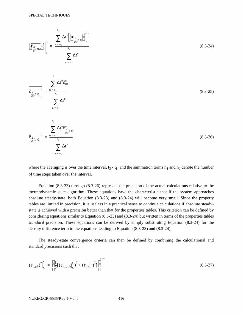
SPECIAL TECHNIQUES
(8.3-24)
(8.3-25)
(8.3-26)
where the averaging is over the time interval, t2 - t1, and the summation terms n1 and n2 denote the number
of time steps taken over the interval.
Equation (8.3-23) through (8.3-26) represent the precision of the actual calculations relative to the
thermodynamic state algorithm. These equations have the characteristic that if the system approaches
absolute steady-state, both Equation (8.3-23) and (8.3-24) will become very small. Since the property
tables are limited in precision, it is useless in a practical sense to continue calculations if absolute steady-
state is achieved with a precision better than that for the properties tables. This criterion can be defined by
considering equations similar to Equation (8.3-23) and (8.3-24) but written in terms of the properties tables
standard precision. These equations can be derived by simply substituting Equation (8.3-24) for the
density difference term in the equations leading to Equation (8.3-23) and (8.3-24).
The steady-state convergence criteria can then be defined by combining the calculational and
standard precisions such that
(8.3-27)
εtd
d ρh( ) 2
t1
t2
∆tn εtd
d ρh( ) 2 n
n n1=
n2
∑
∆tn
n n1=
n2
∑-----------------------------------------------=
δtd
d ρh( )t1
t2
∆tnδρhn
n n1=
n2
∑
∆tn
n n1=
n2
∑--------------------------=
δtd
d ρh( )t1
t2
∆tnδtd
d ρh( )
n
n n1=
n2
∑
∆tn
n n1=
n2
∑--------------------------------=
εc ρh,( )2
t1
t2 12--- εstd ρh, t1
t2( )2
ερh t1
t2( )2
+[ ]
1 2⁄
=
NUREG/CR-5535/Rev 1-Vol I 416

SPECIAL TECHNIQUES
for the system mean enthalpy, and
(8.3-28)
for the system rate of change in enthalpy.
Equation (8.3-27) and (8.3-28) represent the steady-state convergence criterion. It can be said that,
within the limits of calculational and properties precision, time-average steady-state is achieved when the
mean rate of change in system enthalpy is within the limits of
(8.3-29)
where “a” is the mean rate of change in system enthalpy given by Equation (8.3-8). If Equation (8.3-29) is
true and if Equation (8.3-7) is such that
(8.3-30)
then absolute steady-state is achieved. If Equation (8.3-29) is true and
(8.3-31)
then the system is fluctuating and time-average steady-state is achieved.
8.3.3 Steady-State Testing Scheme, Time Interval Control, and Output
In the steady-state testing scheme, the concepts discussed for detecting steady-state are used, and
calculations are performed over time intervals composed of a number of time steps. Because the nature of
each problem is different, a systematic method of varying the test time intervals is performed.
These tests are performed in two parts. First, the system model overall state and rate of change in
state are monitored by evaluating Equation (8.3-1) through (8.3-5) and including these results in the least-
square terms for Equation (8.3-6). At time intervals computed internally, Equation (8.3-6) is evaluated; and
the current system rate of change is determined. If the rate of change in state is increasing, then a divergent
condition is indicated. If the rate of change in state is decreasing or zero, then a convergent condition is
εc
tdd ρh( ),
t2
t2 12--- ε
stdtd
d ρh( ),t1
t2
2
εtd
d ρh( )t1
t2
2
+ 1 2⁄
=
εc
tdd ρh( ),
–t1
t2 a εc
tdd ρh( ),
t2
t2≤ ≤
y εc
tdd ρh( ),
t1
t2≤
y εc
tdd ρh( ),
t1
t2
>
417 NUREG/CR-5535/Rev 1-Vol I
SPECIAL TECHNIQUES
indicated. Second, if a convergent condition is indicated, then calculations are performed to determine the
system average state and average rate of change in state over the internally computed time intervals. These
time-averages are formed by obtaining successive overlapping least-square solutions for Equation (8.3-7).
These successive time-average values are compared, and the achievement or nonachievement of a time-
average steady-state is determined. In performing these tests, the calculational precision is accounted for
by using Equation (8.3-12) through (8.3-29).
In the steady-state scheme, each time a solution for Equation (8.3-6) is obtained, the overall-state and
steady-state convergence test results are printed. This printout is composed of current time results and time
smoothed results integrated over the test time interval. The current time results are (a) the state and rates of
change in state resulting from Equation (8.3-4), (8.3-5), and (8.3-6); (b) the current time uncertainties
resulting from Equation (8.3-18) through (8.3-21); and (c) the current time mean and root mean square
(RMS) mass errors. The time-smoothed results that are printed are the current time evaluation of Equation
(8.3-7) and the resultant coefficients of Equation (8.3-7) determined by the least-squares solution over the
time interval from t1 to the current time TIMEHY. The time, t1, corresponds to the time at the successful
completion of calculations for the first time step after problem initiation. For example, if the problem is a
NEW problem, then t1 corresponds to
t1 = 0 + ∆t1 (8.3-32)
where ∆t1 is the first successful time step. If the problem is a RESTART problem, then t1 corresponds to
t1 = TREST + ∆t (8.3-33)
where TREST is the time of restart and ∆t is the first successful time step after restart. If the results of the
overall state tests indicate a convergent condition, then time-average tests are initiated.
The time-average tests consist of approximating the overall state with a set of three straight lines
where each test line is fitted to the calculational results over successive test intervals. The time rates of
change of these test lines are then monitored to determine time-average steady-state. In the testing scheme,
when the time-average tests are initiated, calculations continue until the successive test time interval is
exceeded. At this time, the first test line, Line A, is defined and its results are printed. Calculations then
continue until the next successive test time interval is exceeded. At this time, the second test line, Line B,
is defined for the second test interval and the third test line, Line C, is defined for the combined first and
second test intervals. The results for the three test lines are then printed, and tests are performed to
determine the achievement of time-average steady-state. If steady-state has not been achieved, then test
Line A is reset to Line B, and the process is repeated until steady-state is achieved.
In the printed edit for time-average steady-state tests, the results for each of the three test lines are
printed. The test line results are obtained by curve fitting Equation (8.3-8) over each of the line test
NUREG/CR-5535/Rev 1-Vol I 418

SPECIAL TECHNIQUES
intervals. The results printed are the endpoints of Equation (8.3-8) evaluated at the test interval start and
end times and the time rate of change of Equation (8.3-8). Also printed are the time-average uncertainties
from Equation (8.3-23) through (8.3-26), the RMS fluctuation of system mean ρh about the line from
Equation (8.3-11), and the mass error integrated over the line test interval.
In performing both the overall and time-average sets of tests, calculations proceed through a logic
scheme to perform tests that monitor the solution scheme’s approach to steady-state. After completing the
logic scheme calculations, the steady-state conclusions and next course of action are printed. This printout
is composed of statements of the mode of convergence and the state of the system in alphanumeric terms.
These statements are defined as the calculations proceed through the logic scheme. To prevent excessive
printout during the overall state convergence tests, the first test for overall convergence is not performed
until the completion of ten successful time steps. At this time, a current test time interval is initialized as
∆tc = TIMEHY - t1. If this test indicates a divergent condition, then the test time interval is increased and
the test procedure is repeated. To increase the test time interval, three tests are performed. First, the current
test time interval is halved and the time t2 is estimated as
(8.3-34)
Then, Equation (8.3-7) is evaluated as y(t2). If y(t2) is greater than the current value of y, then the
time t2 is reset to
t2 = TIMEHY + ∆tc (8.3-35)
and Equation (8.3-7) is reevaluated, which results in resetting y(t2). If y(t2) is again > y, then the time t2 is
again reset to
t2 = TIMEHY + 2∆tc (8.3-36)
In any case, the test time interval is expanded by either maintaining, halving, or doubling the current
test time interval based on a projected estimate of the current time-smoothed convergence function. This
test procedure is then successively repeated until a convergent condition is calculated.
To provide efficiency for the time-average testing scheme, upon the first occurrence of an overall
state convergent condition, the time-average testing scheme is activated and the test time interval is
redefined by estimating the time interval over which a 10% change in state will occur. This time interval is
approximately
(8.3-37)
t2 TIMEHY12---∆tc+=
∆tc 0.1 ρh( )ny⁄∼
419 NUREG/CR-5535/Rev 1-Vol I
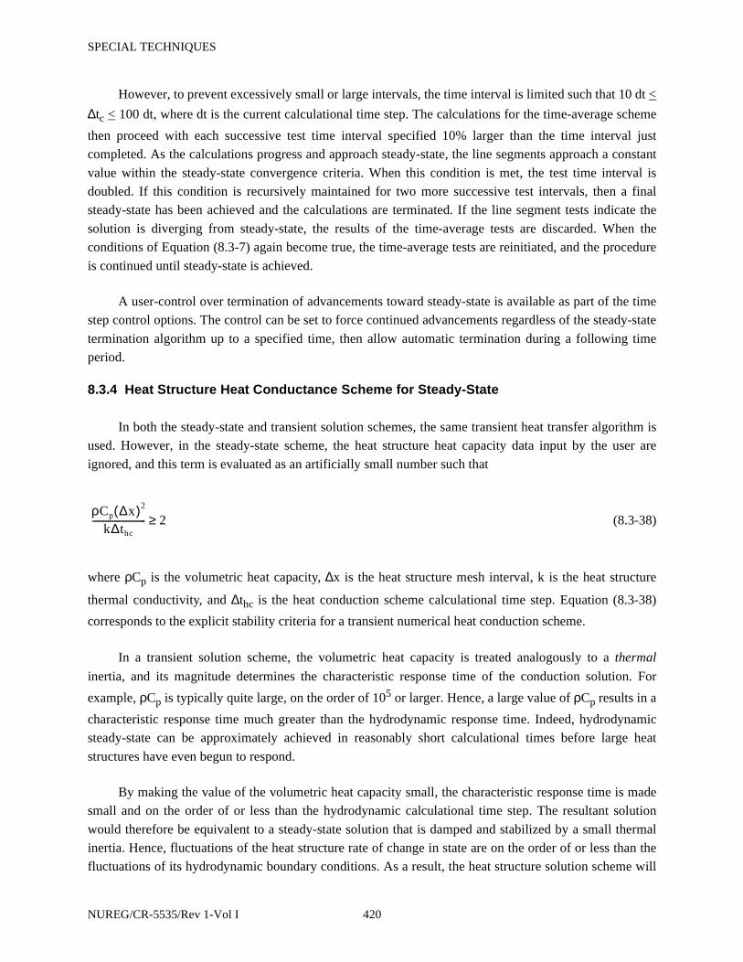
SPECIAL TECHNIQUES
However, to prevent excessively small or large intervals, the time interval is limited such that 10 dt <
∆tc < 100 dt, where dt is the current calculational time step. The calculations for the time-average scheme
then proceed with each successive test time interval specified 10% larger than the time interval just
completed. As the calculations progress and approach steady-state, the line segments approach a constant
value within the steady-state convergence criteria. When this condition is met, the test time interval is
doubled. If this condition is recursively maintained for two more successive test intervals, then a final
steady-state has been achieved and the calculations are terminated. If the line segment tests indicate the
solution is diverging from steady-state, the results of the time-average tests are discarded. When the
conditions of Equation (8.3-7) again become true, the time-average tests are reinitiated, and the procedure
is continued until steady-state is achieved.
A user-control over termination of advancements toward steady-state is available as part of the time
step control options. The control can be set to force continued advancements regardless of the steady-state
termination algorithm up to a specified time, then allow automatic termination during a following time
period.
8.3.4 Heat Structure Heat Conductance Scheme for Steady-State
In both the steady-state and transient solution schemes, the same transient heat transfer algorithm is
used. However, in the steady-state scheme, the heat structure heat capacity data input by the user are
ignored, and this term is evaluated as an artificially small number such that
(8.3-38)
where ρCp is the volumetric heat capacity, ∆x is the heat structure mesh interval, k is the heat structure
thermal conductivity, and ∆thc is the heat conduction scheme calculational time step. Equation (8.3-38)
corresponds to the explicit stability criteria for a transient numerical heat conduction scheme.
In a transient solution scheme, the volumetric heat capacity is treated analogously to a thermal
inertia, and its magnitude determines the characteristic response time of the conduction solution. For
example, ρCp is typically quite large, on the order of 105 or larger. Hence, a large value of ρCp results in a
characteristic response time much greater than the hydrodynamic response time. Indeed, hydrodynamic
steady-state can be approximately achieved in reasonably short calculational times before large heat
structures have even begun to respond.
By making the value of the volumetric heat capacity small, the characteristic response time is made
small and on the order of or less than the hydrodynamic calculational time step. The resultant solution
would therefore be equivalent to a steady-state solution that is damped and stabilized by a small thermal
inertia. Hence, fluctuations of the heat structure rate of change in state are on the order of or less than the
fluctuations of its hydrodynamic boundary conditions. As a result, the heat structure solution scheme will
ρCp ∆x( )2
k∆thc------------------------ 2≥
NUREG/CR-5535/Rev 1-Vol I 420

SPECIAL TECHNIQUES
achieve time-average steady-state at approximately the same time as time-average hydrodynamic steady-
state.
8.3.5 Interrelationship of Steady-State and Transient Restart/Plot Records
During the course of the calculations, restart/plot records are written at the frequency specified by the
user. When the code determines that steady-state has been achieved, a restart/plot record is written
unconditionally. Subsequent problems can then be run as restarts using any of these restart records.
However, the code will treat the restart records differently, depending on the type of problem using the
restart record.
If a transient problem is being run by restarting from a steady-state restart record or, conversely, if a
steady-state problem is being run restarting from a transient restart record, the restart is treated as a new
problem. In this case, only the restart record at which the problem restarts is written and used for initial
conditions. The code time step counters, statistics, and problem simulation time are reset to zero, and
additional restart/plot records are written as the problem progresses.
If a steady-state problem is being run restarting from a steady-state restart record or, conversely, if a
transient problem is being run restarting from a transient restart record, then the restart is treated as a
continuation of the problem. In the continuation case, the previous restart/plot records up to the point of
restart are preserved; and additional records are written as the problem progresses.
8.4 Self-Initialization
8.4.1 General Description
Obtaining a desired, steady-state condition for a RELAP5 plant model often requires considerable
time and effort on the part of the analyst. Typically, this process involves successive calculations involving
a trial-and-error approach in adjusting various input data. While the RELAP5 code can compute a steady-
state condition for a particular set of boundary conditions, this steady-state may not match all parameters
measured in the plant due to the particular nodalization chosen by the analyst, inherent inaccuracies in
code models of the physical processes, inability to model geometric details, etc. The self-initialization
option is designed to reduce the time, effort, and cost to achieve a steady-state for a given RELAP5 plant
model to more nearly match plant data if necessary.
The strategy of the scheme is to automate the control aspects of the problem and to significantly
reduce the computational time needed to reach a steady-state. The concept retains the conventional
approach of conducting a transient calculation that is driven to a desired steady-state condition.
Automation of plant model control is effected by a generic set of controllers that mimic an actual
plant control system. These controllers are control components defined by the user. Four suboptions are
permitted with respect to the definition of independent and dependent plant model parameters. The choice
of suboptions affords the user flexibility in meeting particular analysis objectives. Moreover, the overall
421 NUREG/CR-5535/Rev 1-Vol I

SPECIAL TECHNIQUES
scheme has been designed such that the user may invoke a standard control package or opt to custom-tailor
the new control components to suit a particular plant model.
A reduction in calculational computer time to perform the initialization is accomplished by using the
steady-state and nearly-implicit solution scheme options (see Section 8.3 and Section 3.1.5, respectively).
The steady-state option diminishes thermal capacitance terms to lower stability limits, thereby
significantly reducing thermal relaxation of the model. It also monitors for a steady-state condition. The
nearly-implicit solution scheme permits time steps larger than those implied by the material Courant limit.
The self-initialization option is described for PWR-type models employing either U-tube or once-
through steam generators and of single- or multiple-loop design. However, the principles illustrated can be
applied to other systems.
8.4.2 Required Plant Model Characteristics
The option accommodates plant models representing all domestically produced PWR designs, i.e.,
those of Westinghouse, Combustion Engineering, and Babcock & Wilcox. More specifically, single-loop,
two-loop, three-loop, four-loop, and 2 x 4 loop representations are accommodated, using either U-tube or
once-through steam generators. Other assumptions and restrictions related to the plant model are as
follows:
• The model must have at least one coolant loop consisting of a core region, pump, steamgenerator, and pressurizer.
• The core power must be constant or it too must be driven by a control system to constantpower. The reactor kinetics model may be used and held to constant input power by notentering feedback data. Reactor kinetics data with feedback needed for the transient canbe entered at the restart starting the transient.
• User-specified makeup and letdown flow modeling should be suppressed during the nulltransient. The same applies to pressurizer heater and spray modeling. They may beintroduced into the model as a renodalization at transient initiation. Volume and pressurecontrol during the null transient must be effected through a time-dependent volume thatserves to replace the pressurizer.
• Self-initialization of the plant model encompasses the primary coolant system and steamgenerators under the standard approach described subsequently. That is, no provisionshave been made to include the balance-of-plant components in the testing for a steady-state, though this is possible and is not incompatible with the self-initialization option.However, if the plant model includes a balance-of-plant representation (e.g., turbine,condensers, feedwater pumps, feedwater heaters, etc.), appropriate controllers wouldhave to be supplied by the user to govern the operation of these components.
• The option is executable from either a new problem data deck or the restart of an oldproblem.
NUREG/CR-5535/Rev 1-Vol I 422
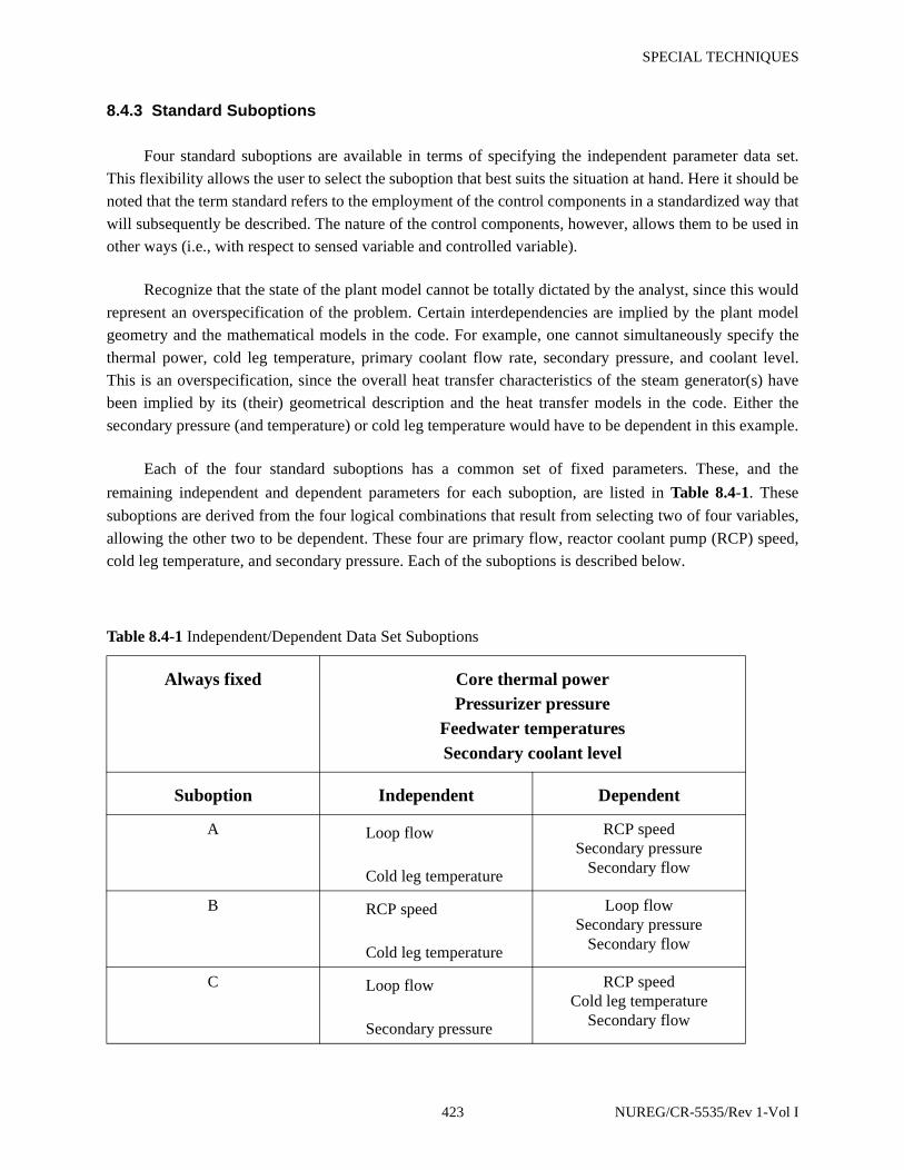
SPECIAL TECHNIQUES
8.4.3 Standard Suboptions
Four standard suboptions are available in terms of specifying the independent parameter data set.
This flexibility allows the user to select the suboption that best suits the situation at hand. Here it should be
noted that the term standard refers to the employment of the control components in a standardized way that
will subsequently be described. The nature of the control components, however, allows them to be used in
other ways (i.e., with respect to sensed variable and controlled variable).
Recognize that the state of the plant model cannot be totally dictated by the analyst, since this would
represent an overspecification of the problem. Certain interdependencies are implied by the plant model
geometry and the mathematical models in the code. For example, one cannot simultaneously specify the
thermal power, cold leg temperature, primary coolant flow rate, secondary pressure, and coolant level.
This is an overspecification, since the overall heat transfer characteristics of the steam generator(s) have
been implied by its (their) geometrical description and the heat transfer models in the code. Either the
secondary pressure (and temperature) or cold leg temperature would have to be dependent in this example.
Each of the four standard suboptions has a common set of fixed parameters. These, and the
remaining independent and dependent parameters for each suboption, are listed in Table 8.4-1. These
suboptions are derived from the four logical combinations that result from selecting two of four variables,
allowing the other two to be dependent. These four are primary flow, reactor coolant pump (RCP) speed,
cold leg temperature, and secondary pressure. Each of the suboptions is described below.
Table 8.4-1 Independent/Dependent Data Set Suboptions
Always fixed Core thermal powerPressurizer pressure
Feedwater temperaturesSecondary coolant level
Suboption Independent Dependent
A Loop flow
Cold leg temperature
RCP speedSecondary pressure
Secondary flow
B RCP speed
Cold leg temperature
Loop flowSecondary pressure
Secondary flow
C Loop flow
Secondary pressure
RCP speedCold leg temperature
Secondary flow
423 NUREG/CR-5535/Rev 1-Vol I

SPECIAL TECHNIQUES
8.4.3.1 Suboption A.
Loop flow and cold leg temperature are specified. (Note that specification of primary flow, core
thermal power, and primary pressure fixes the differential temperature across the vessel.a) This suboption
requires that the pump speed, secondary pressure, and secondary feedwater flow be dependent variables.
The pump speed (N) is determined based on loop flow ( ), loop pressure drop (∆P), and the pump
characteristics, as determined from pump model input. That is,
(8.4-1)
Here it should be noted that the resulting pump speed may be different than an observed value (in the
case of an experimental facility) or the synchronous speed (in the case of a full-scale plant). This merely
implies that a mismatch is present in the input data. For example, the user-specified geometry and/or loss
coefficients for the primary coolant system (PCS) may be inaccurate, and/or the pump model may be
inaccurate. The analyst must resolve such inconsistencies. The code will not alter either the pump model or
loss coefficients to arrive at a flow/speed combination that matches facility data.
Analogously, specifying the cold leg temperature (along with power and loop flow) requires that the
secondary pressure and flow must be dependent. The secondary pressure dictates the secondary sink
temperature and, therefore, the primary-to-secondary heat transfer potential and cold leg temperature. Here
again, it should be noted that the resulting secondary pressure may not match that observed in the plant or
test facility. This may mean one of two things. Either the plant model representation of the steam generator
is inadequate (e.g., inaccurately modeled, improperly nodalized, etc.), or the physical models in the code
are imprecise. For example, the failure to match a measured value of secondary pressure might be due to
the fact that the tube fouling was not accounted for in the input model.
D RCP speed
Secondary pressure
Loop flowCold leg temperature
Secondary flow
a. This takes into account the total pump power and heat losses as well.
Table 8.4-1 Independent/Dependent Data Set Suboptions (Continued)
Always fixed Core thermal powerPressurizer pressure
Feedwater temperaturesSecondary coolant level
m·
N f m· ∆P,( )=
NUREG/CR-5535/Rev 1-Vol I 424
SPECIAL TECHNIQUES
8.4.3.2 Suboption B.
RCP speed and cold leg temperature are specified, while loop flow, secondary pressure, and
secondary flow are dependent. This suboption is similar to suboption A except that the roles of RCP speed
and loop flow as dependent and independent variables are reversed. This suboption would be desirable
when modeling a plant for which no data exist but the synchronous pump speed is known.
8.4.3.3 Suboption C.
Loop flow and secondary pressure are specified, while RCP speed, cold leg temperature, and
secondary flow are dependent. This suboption is desirable when secondary pressure matching (to data)
would play an important role in the transient.
8.4.3.4 Suboption D.
RCP speed and secondary pressure are specified, while loop flow, cold leg temperature, and
secondary flow are dependent. This suboption is similar to suboption C, except that the independent/
dependent roles of loop flow and pump speed are reversed.
8.4.4 Inherent Model Incompatibilities
With such generality possible in defining a plant model with RELAP5, it is clearly possible that a
desired steady-state condition is impossible to achieve given the input data supplied. Several types of
incompatibilities will not be readily apparent until a null transient is attempted. For example, the overall
heat transfer capacity of the steam generator(s) may be insufficient to transfer the total core thermal power
without causing the hot leg temperature to exceed TSAT. Such anomalies will be obvious as the null
transient proceeds but cannot be readily identified from the input data stream.
8.4.5 Description of Standard Controllers
To effect overall control of the model during the null transient, three generic control components are
available and are used to invoke any one of the four suboptions just described. These control components
are identified as PUMPCTL, STEAMCTL, and FEEDCTL. For all suboptions, both STEAMCTL and
FEEDCTL are needed; whereas, PUMPCTL is used only for suboptions A and C where loop flow control
is desired. The following subsections describe the design and operation of the controllers.
8.4.5.1 PUMPCTL Controller.
The standard use of the PUMPCTL component is to sense loop flow and control pump speed to
achieve the desired flow rate. As is the case with the other controllers, it uses proportional and integral
control. Through input, the user specifies (among other things) the desired flow rate, where the flow is to
be sensed, and which pump is to be controlled. The mathematical expressions representing the operation of
the controller are next described.
425 NUREG/CR-5535/Rev 1-Vol I
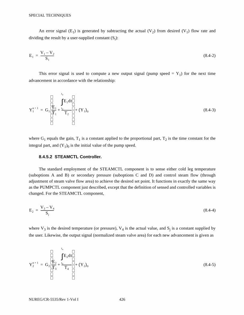
SPECIAL TECHNIQUES
An error signal (E1) is generated by subtracting the actual (V2) from desired (V1) flow rate and
dividing the result by a user-supplied constant (Si):
(8.4-2)
This error signal is used to compute a new output signal (pump speed = Y1) for the next time
advancement in accordance with the relationship:
(8.4-3)
where G1 equals the gain, T1 is a constant applied to the proportional part, T2 is the time constant for the
integral part, and (Y1)0 is the initial value of the pump speed.
8.4.5.2 STEAMCTL Controller.
The standard employment of the STEAMCTL component is to sense either cold leg temperature
(suboptions A and B) or secondary pressure (suboptions C and D) and control steam flow (through
adjustment of steam valve flow area) to achieve the desired set point. It functions in exactly the same way
as the PUMPCTL component just described, except that the definition of sensed and controlled variables is
changed. For the STEAMCTL component,
(8.4-4)
where V3 is the desired temperature (or pressure), V4 is the actual value, and Sj is a constant supplied by
the user. Likewise, the output signal (normalized steam valve area) for each new advancement is given as
(8.4-5)
E1
V1 V2–S1
------------------=
Y1n 1+ G1
E1
T1-----
E1dt
t0
tn
∫T2
--------------+
Y1( )0+=
E2
V3 V4–Sj
------------------=
Y2n 1+ G2
E2
T3-----
E2dt
t0
tn
∫T4
--------------+
Y2( )0+=
NUREG/CR-5535/Rev 1-Vol I 426

SPECIAL TECHNIQUES
where the terms are analogous to those for the PUMPCTL component.
8.4.5.3 FEEDCTL Controller.
The standard employment of the FEEDCTL component is to sense steam flow and steam generator
secondary coolant level (or coolant mass) and control feedwater flow (through adjustment of feedwater
valve flow area) to achieve a match between feedwater flow and steam flow and to achieve the desired
coolant level (or mass). It is also a proportional/integral controller but uses a summed error signal made up
of the individual flow and level (mass) errors:
(8.4-6)
where
V5 = desired level (mass)
V6 = actual level (mass)
Sk = user-supplied constant
V7 = actual steam flow
V8 = actual feedwater flow
Sm = user-supplied constant
The output signal (feedwater valve flow area) is computed analogously to the PUMPCTL and
STEAMCTL components:
(8.4-7)
8.4.5.4 Pressure and Volume Control.
The self-initialization option requires that a constant pressure boundary condition be imposed on the
primary coolant system during the null transient. The user supplies this condition by adding a time-
dependent volume as a replacement for the pressurizer. This time-dependent volume should be defined as
E3
V5 V6–Sk
------------------V7 V8–
Sm------------------+=
Y3n 1+ G3
E3
T5-----
E3dt
t0
tn
∫T6
--------------+
Y3( )0+=
427 NUREG/CR-5535/Rev 1-Vol I

SPECIAL TECHNIQUES
containing liquid at the desired primary system pressure and at a temperature near that estimated to be the
final hot leg temperature. During the null transient, liquid will either flow into or out of the time-dependent
volume to accommodate expansion and shrinkage, with no attendant change in primary pressure. When the
self-initialization option is invoked, the code will check to determine if the time-dependent volume has
been included.
NUREG/CR-5535/Rev 1-Vol I 428