Reinforcement learning - LTHfileadmin.cs.lth.se/.../EDA132/Slides/ReinforcementLearning.pdf ·...
126
Reinforcement learning Applied artificial intelligence (EDA132) Lecture 13 2012-04-26 Elin A. Topp Material based on course book, chapter 21 (17), and on lecture “Belöningsbaserad inlärning / Reinforcement learning” by Örjan Ekeberg, CSC/Nada, KTH, autumn term 2006 (in Swedish) 1 Friday, 27 April 2012
Transcript of Reinforcement learning - LTHfileadmin.cs.lth.se/.../EDA132/Slides/ReinforcementLearning.pdf ·...
Reinforcement learning
Applied artificial intelligence (EDA132)Lecture 132012-04-26Elin A. Topp
Material based on course book, chapter 21 (17), and on lecture “Belöningsbaserad inlärning / Reinforcement learning” by Örjan Ekeberg, CSC/Nada, KTH, autumn term 2006 (in Swedish)
1Friday, 27 April 2012

Outline• Reinforcement learning (chapter 21, with some references to 17)
• Problem definition
• Learning situation
• Roll of the reward
• Simplified assumptions
• Central concepts and terms
• Known environment
• Bellman’s equation
• Approaches to solutions
• Unknown environment
• Monte-Carlo method
• Temporal-Difference learning
• Q-Learning
• Sarsa-Learning
• Improvements
• The usefulness of making mistakes
• Eligibility Trace
2Friday, 27 April 2012

Outline• Reinforcement learning (chapter 21, with some references to 17)
• Problem definition
• Learning situation
• Roll of the reward
• Simplified assumptions
• Central concepts and terms
• Known environment
• Bellman’s equation
• Approaches to solutions
• Unknown environment
• Monte-Carlo method
• Temporal-Difference learning
• Q-Learning
• Sarsa-Learning
• Improvements
• The usefulness of making mistakes
• Eligibility Trace
3Friday, 27 April 2012
Reinforcement learning
Learning of a behaviour (a strategy, a skill) without access to a right / wrong measure for actions and decisions taken.
4Friday, 27 April 2012
Reinforcement learning
Learning of a behaviour (a strategy, a skill) without access to a right / wrong measure for actions and decisions taken.
With the help of a reward, a measure is given, of how well things are going
4Friday, 27 April 2012

Reinforcement learning
Learning of a behaviour (a strategy, a skill) without access to a right / wrong measure for actions and decisions taken.
With the help of a reward, a measure is given, of how well things are going
Note: The reward is not given in direct connection with a good choice of action (temporal credit assignment)
Note: The reward does not tell what exactly it was, that made the “good” action(structural credit assignment)
4Friday, 27 April 2012
Real life examples
5Friday, 27 April 2012

Real life examples
5
Riding a bicycle
Powder skiing
Friday, 27 April 2012

Learning situation: A modelAn agent interacts with its environment
The agent performs actions
Actions have influence on the environment’s state
The agent observes the environment’s state and receives a reward from the environment
6
Agent EnvironmentAction a
State s
Reward r
Friday, 27 April 2012

Learning situation: The agent’s taskThe task:
Find a behaviour (action sequence) that maximises the overall reward
How long into the future should we spy?
Finite time horizon:
max E[ ∑ rt]
Infinite time horizon:
max E[ ∑ γt rt]
with γ being a discount factor for future rewards (0 < γ < 1)
7
h
t=0
∞t=0
Friday, 27 April 2012
The reward function’s roll
The reward function depends on the type of task
8Friday, 27 April 2012

The reward function’s roll
The reward function depends on the type of task
• Game (Chess, Backgammon): Reward is given only in the end of the game, +1 for “win”, -1 for “loose”
8Friday, 27 April 2012

The reward function’s roll
The reward function depends on the type of task
• Game (Chess, Backgammon): Reward is given only in the end of the game, +1 for “win”, -1 for “loose”
• Avoid mistakes (Riding a bike, Learning to fly according to hitchhiker’s guide): Reward -1 when failing (falling)
8Friday, 27 April 2012
The reward function’s roll
The reward function depends on the type of task
• Game (Chess, Backgammon): Reward is given only in the end of the game, +1 for “win”, -1 for “loose”
• Avoid mistakes (Riding a bike, Learning to fly according to hitchhiker’s guide): Reward -1 when failing (falling)
• Find the shortest / cheapest / fastest path to a goal: Reward -1 for each step
8Friday, 27 April 2012

A classic example: Grid World
Simplified “Wumpus world” with just two gold pieces
9
G
G
Friday, 27 April 2012

A classic example: Grid World
Simplified “Wumpus world” with just two gold pieces
• Every state sj is represented by a field in the grid
9
G
G
Friday, 27 April 2012

A classic example: Grid World
Simplified “Wumpus world” with just two gold pieces
• Every state sj is represented by a field in the grid
• Action a the agent can choose consists of moving one step to a neighbouring field
9
G
G
Friday, 27 April 2012

A classic example: Grid World
Simplified “Wumpus world” with just two gold pieces
• Every state sj is represented by a field in the grid
• Action a the agent can choose consists of moving one step to a neighbouring field
• Reward: -1 in every step until one of the goals (G) is reached.
9
G
G
Friday, 27 April 2012

Simplifying assumptions
10Friday, 27 April 2012
Simplifying assumptions
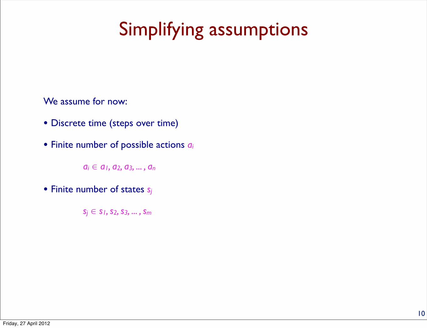
We assume for now:
10Friday, 27 April 2012

Simplifying assumptions
We assume for now:
• Discrete time (steps over time)
10Friday, 27 April 2012

Simplifying assumptions
We assume for now:
• Discrete time (steps over time)
• Finite number of possible actions ai
ai ∈ a1, a2, a3, ... , an
10Friday, 27 April 2012
Simplifying assumptions
We assume for now:
• Discrete time (steps over time)
• Finite number of possible actions ai
ai ∈ a1, a2, a3, ... , an
• Finite number of states sj
sj ∈ s1, s2, s3, ... , sm
10Friday, 27 April 2012

Simplifying assumptions
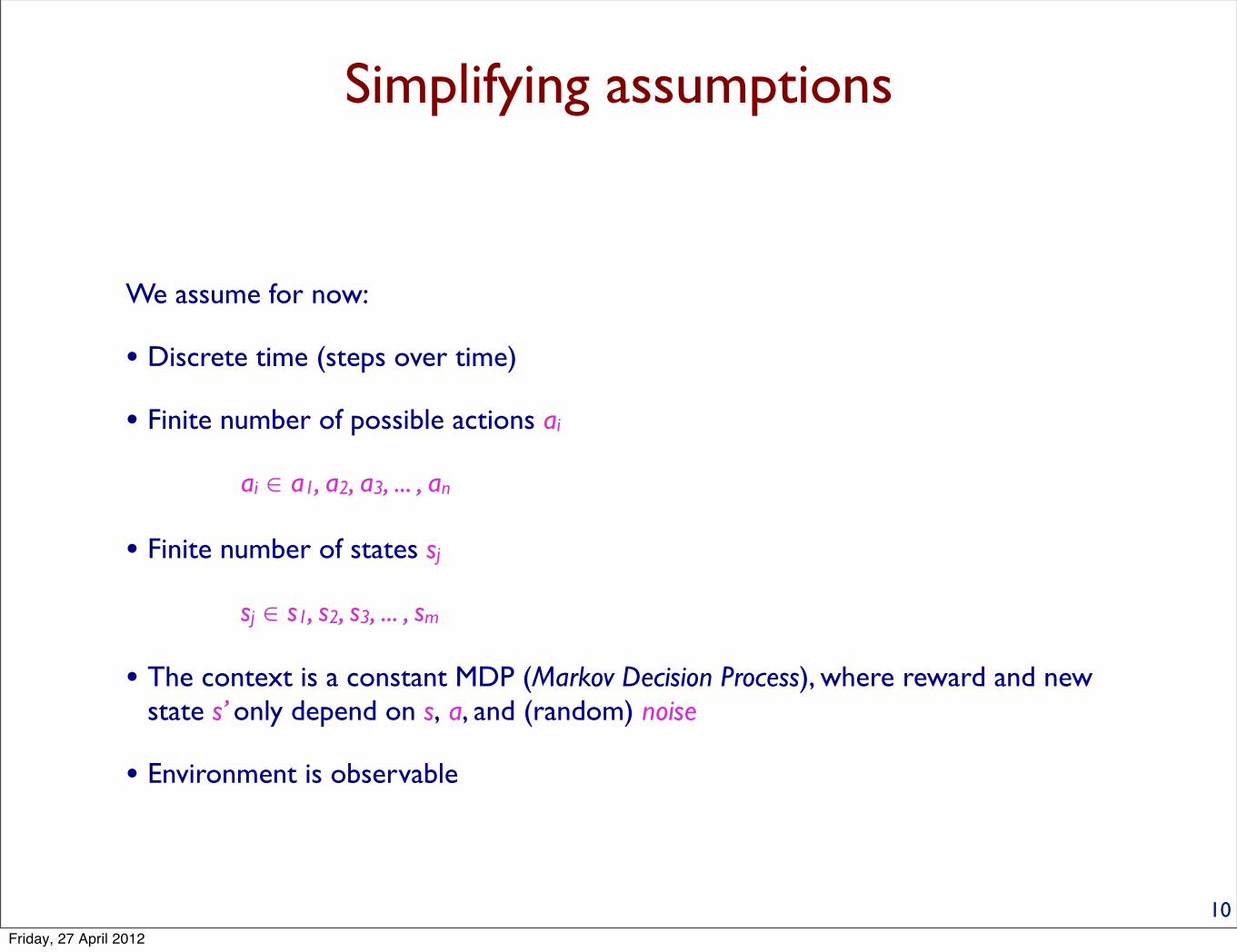
We assume for now:
• Discrete time (steps over time)
• Finite number of possible actions ai
ai ∈ a1, a2, a3, ... , an
• Finite number of states sj
sj ∈ s1, s2, s3, ... , sm
• The context is a constant MDP (Markov Decision Process), where reward and new state s’ only depend on s, a, and (random) noise
10Friday, 27 April 2012
Simplifying assumptions
We assume for now:
• Discrete time (steps over time)
• Finite number of possible actions ai
ai ∈ a1, a2, a3, ... , an
• Finite number of states sj
sj ∈ s1, s2, s3, ... , sm
• The context is a constant MDP (Markov Decision Process), where reward and new state s’ only depend on s, a, and (random) noise
• Environment is observable
10Friday, 27 April 2012
The agent’s internal representation
11Friday, 27 April 2012

The agent’s internal representation
• An agent’s policy π is the “rule” after which the agent chooses its action a in a given state s
π(s) ⟼ a
11Friday, 27 April 2012

The agent’s internal representation
• An agent’s policy π is the “rule” after which the agent chooses its action a in a given state s
π(s) ⟼ a
• An agent’s utility function U describes the expected future reward given s, when following policy π
Uπ(s) ⟼ ℜ
11Friday, 27 April 2012

Grid World: A state’s value
A state’s value depends on the chosen policy
12Friday, 27 April 2012

Grid World: A state’s value
A state’s value depends on the chosen policy
12
0 -1 -2 -3
-1 -2 -3 -2
-2 -3 -2 -1
-3 -2 -1 0
U with optimal policy
Friday, 27 April 2012

Grid World: A state’s value
A state’s value depends on the chosen policy
12
0 -1 -2 -3
-1 -2 -3 -2
-2 -3 -2 -1
-3 -2 -1 0
U with optimal policy
0 -14 -20 -22
-14 -18 -22 -20
-20 -22 -18 -14
-22 -20 -14 0
U with random policy
Friday, 27 April 2012

A 4x3 world
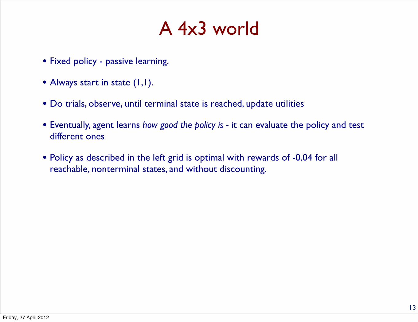
• Fixed policy - passive learning.
13Friday, 27 April 2012

A 4x3 world
• Fixed policy - passive learning.
• Always start in state (1,1).
13Friday, 27 April 2012

A 4x3 world
• Fixed policy - passive learning.
• Always start in state (1,1).
• Do trials, observe, until terminal state is reached, update utilities
13Friday, 27 April 2012
A 4x3 world
• Fixed policy - passive learning.
• Always start in state (1,1).
• Do trials, observe, until terminal state is reached, update utilities
• Eventually, agent learns how good the policy is - it can evaluate the policy and test different ones
13Friday, 27 April 2012
A 4x3 world
• Fixed policy - passive learning.
• Always start in state (1,1).
• Do trials, observe, until terminal state is reached, update utilities
• Eventually, agent learns how good the policy is - it can evaluate the policy and test different ones
• Policy as described in the left grid is optimal with rewards of -0.04 for all reachable, nonterminal states, and without discounting.
13Friday, 27 April 2012

A 4x3 world
• Fixed policy - passive learning.
• Always start in state (1,1).
• Do trials, observe, until terminal state is reached, update utilities
• Eventually, agent learns how good the policy is - it can evaluate the policy and test different ones
• Policy as described in the left grid is optimal with rewards of -0.04 for all reachable, nonterminal states, and without discounting.
13
R R R +1
U U -1
U L L L
Friday, 27 April 2012
A 4x3 world
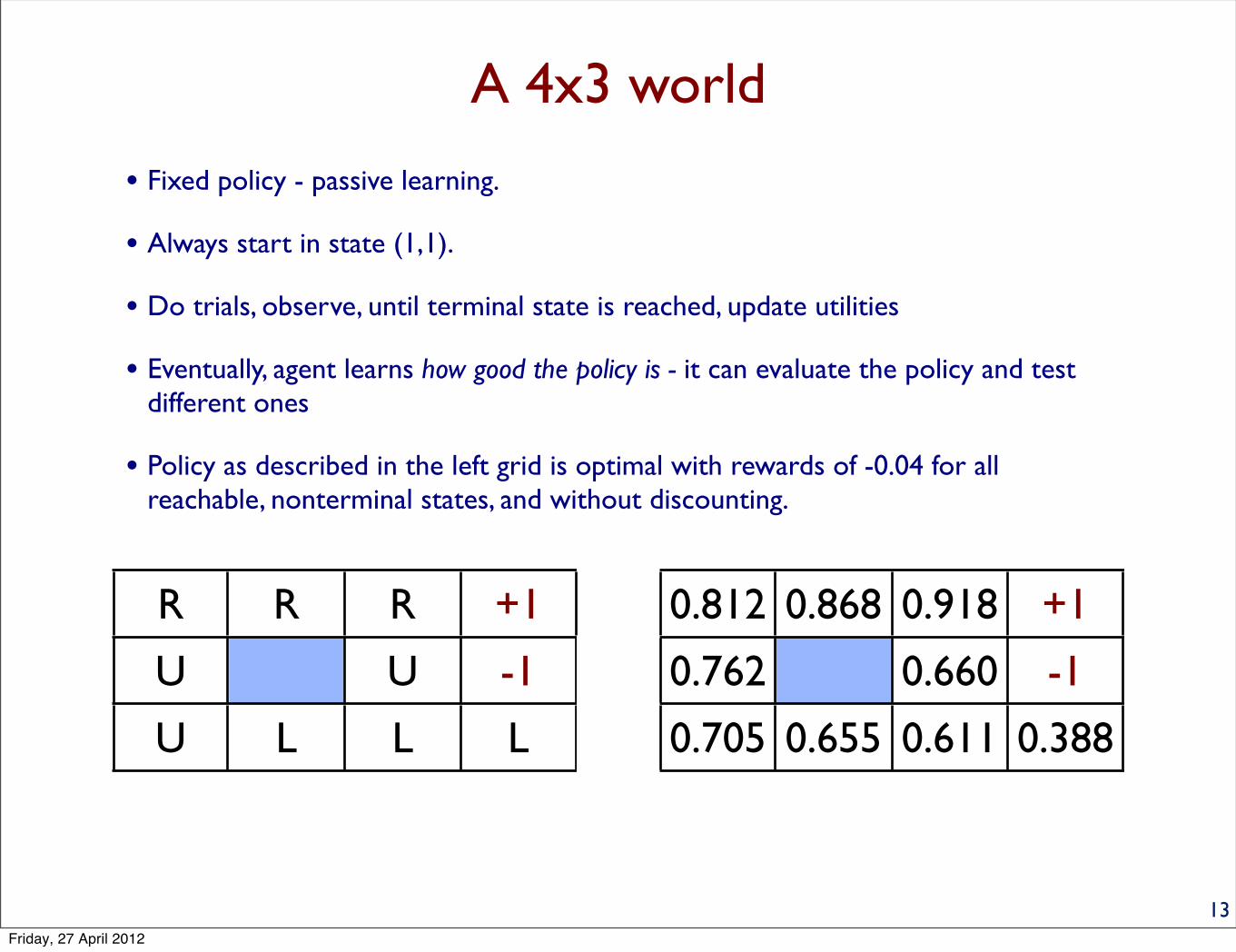
• Fixed policy - passive learning.
• Always start in state (1,1).
• Do trials, observe, until terminal state is reached, update utilities
• Eventually, agent learns how good the policy is - it can evaluate the policy and test different ones
• Policy as described in the left grid is optimal with rewards of -0.04 for all reachable, nonterminal states, and without discounting.
13
R R R +1
U U -1
U L L L
0.812 0.868 0.918 +1
0.762 0.660 -1
0.705 0.655 0.611 0.388
Friday, 27 April 2012

Outline• Reinforcement learning (chapter 21, with some references to 17)
• Problem definition
• Learning situation
• Roll of the reward
• Simplified assumptions
• Central concepts and terms
• Known (observable) environment
• Bellman’s equation
• Approaches to solutions
• Unknown environment
• Monte-Carlo method
• Temporal-Difference learning
• Q-Learning
• Sarsa-Learning
• Improvements
• The usefulness of making mistakes
• Eligibility Trace
14Friday, 27 April 2012

Environment model
15Friday, 27 April 2012

Environment model
•Where do we get in each step?
δ(s, a) ⟼ s’
15Friday, 27 April 2012

Environment model
•Where do we get in each step?
δ(s, a) ⟼ s’
•What will the reward be?
r( s, a) ⟼ ℜ
15Friday, 27 April 2012

Environment model
•Where do we get in each step?
δ(s, a) ⟼ s’
•What will the reward be?
r( s, a) ⟼ ℜ
15Friday, 27 April 2012

Environment model
•Where do we get in each step?
δ(s, a) ⟼ s’
•What will the reward be?
r( s, a) ⟼ ℜ
The utility values of different states obey Bellman’s equation, given a fixed policy π:
Uπ(s) = r( s, π(s)) + γ·Uπ( δ( s, π(s)))
15Friday, 27 April 2012

Solving the equation
16Friday, 27 April 2012

Solving the equation
There are two ways of solving Bellman’s equation
Uπ(s) = r( s, π(s)) + γ·Uπ( δ( s, π(s)))
16Friday, 27 April 2012

Solving the equation
There are two ways of solving Bellman’s equation
Uπ(s) = r( s, π(s)) + γ·Uπ( δ( s, π(s)))
• Directly: Uπ(s) = r( s, π(s)) + γ·∑s’ P( s’ | s, π(s)) Uπ(s’)
16Friday, 27 April 2012

Recap: Random policy
17
0 -14 -20 -22
-14 -18 -22 -20
-20 -22 -18 -14
-22 -20 -14 0
Uπ(s) = r( s, π(s)) + γ·∑s’ P( s’ | s, π(s)) Uπ(s’)
Friday, 27 April 2012
Solving the equation
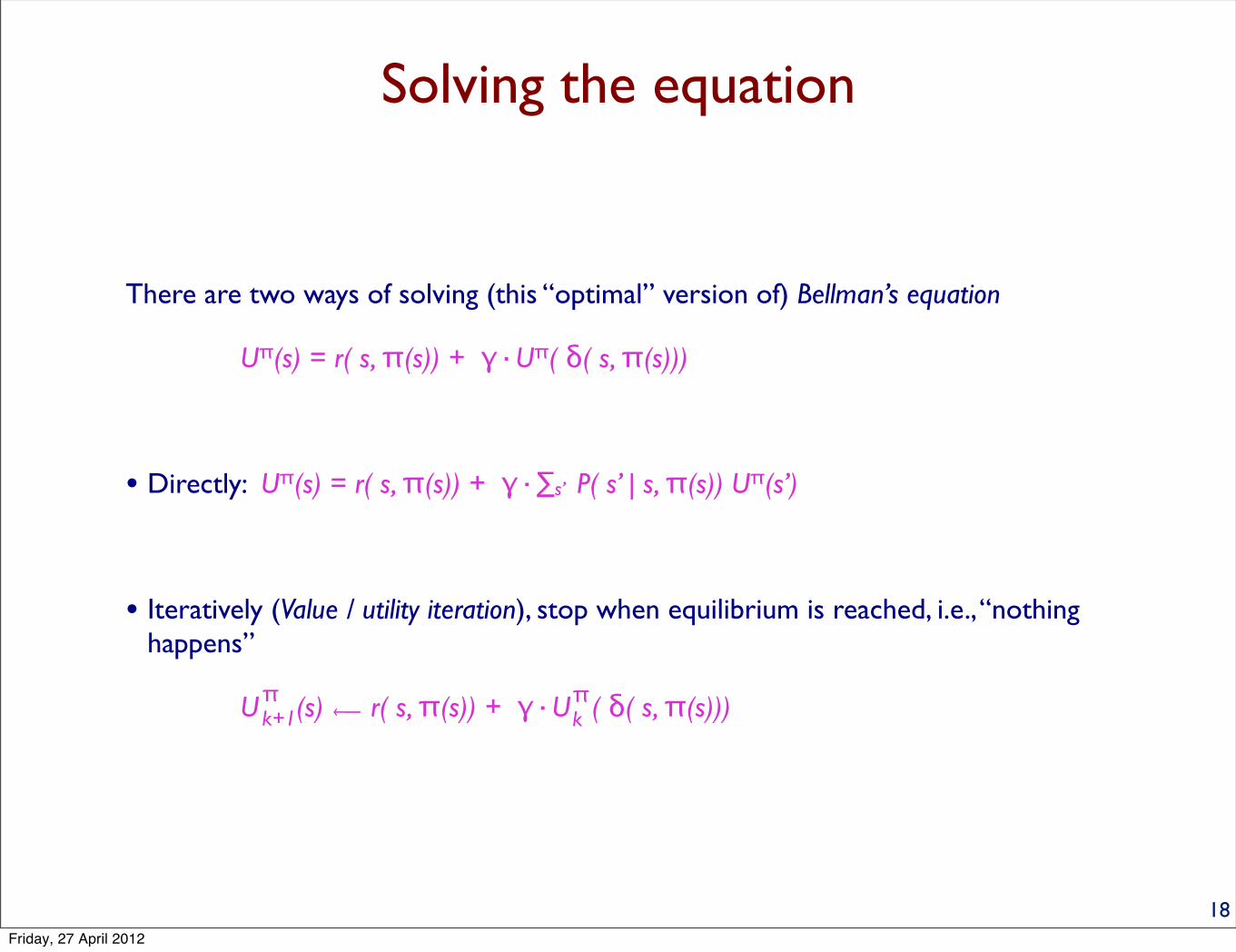
There are two ways of solving (this “optimal” version of) Bellman’s equation
Uπ(s) = r( s, π(s)) + γ·Uπ( δ( s, π(s)))
• Directly: Uπ(s) = r( s, π(s)) + γ·∑s’ P( s’ | s, π(s)) Uπ(s’)
• Iteratively (Value / utility iteration), stop when equilibrium is reached, i.e., “nothing happens”
U (s) ⟵ r( s, π(s)) + γ·U ( δ( s, π(s)))
18
πk+1
πk
Friday, 27 April 2012
Bayesian reinforcement learning
19Friday, 27 April 2012
Bayesian reinforcement learning
A remark:
19Friday, 27 April 2012
Bayesian reinforcement learning
A remark:
One form of reinforcement learning integrates Bayesian learning into the process to obtain the transition model, i.e., P( s’ | s, π(s))
19Friday, 27 April 2012
Bayesian reinforcement learning
A remark:
One form of reinforcement learning integrates Bayesian learning into the process to obtain the transition model, i.e., P( s’ | s, π(s))
This means to assume a prior probability for each hypothesis on how the model might look like and then applying Bayes’ rule to obtain the posterior.
19Friday, 27 April 2012

Bayesian reinforcement learning
A remark:
One form of reinforcement learning integrates Bayesian learning into the process to obtain the transition model, i.e., P( s’ | s, π(s))
This means to assume a prior probability for each hypothesis on how the model might look like and then applying Bayes’ rule to obtain the posterior.
We are not going into details here!
19Friday, 27 April 2012

Finding optimal policy and value function
20Friday, 27 April 2012
Finding optimal policy and value function
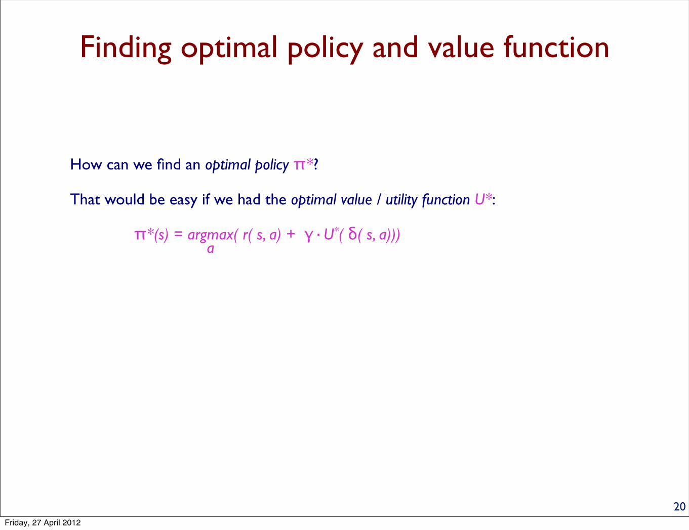
How can we find an optimal policy π*?
20Friday, 27 April 2012
Finding optimal policy and value function
How can we find an optimal policy π*?
That would be easy if we had the optimal value / utility function U*:
π*(s) = argmax( r( s, a) + γ·U*( δ( s, a))) a
20Friday, 27 April 2012

Finding optimal policy and value function
How can we find an optimal policy π*?
That would be easy if we had the optimal value / utility function U*:
π*(s) = argmax( r( s, a) + γ·U*( δ( s, a))) a
Apply to the “optimal version” of Bellman’s equation
U*(s) = max( r( s, a) + γ·U*( δ( s, a))) a
Tricky to solve ... but possible:
Combine policy and value iteration by switching in each iteration step
20Friday, 27 April 2012

Policy iteration
21Friday, 27 April 2012

Policy iteration
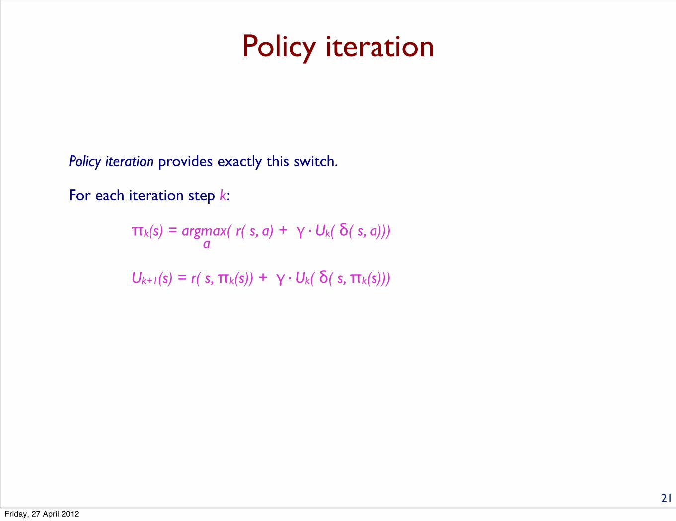
Policy iteration provides exactly this switch.
21Friday, 27 April 2012
Policy iteration
Policy iteration provides exactly this switch.
For each iteration step k:
πk(s) = argmax( r( s, a) + γ·Uk( δ( s, a))) a
Uk+1(s) = r( s, πk(s)) + γ·Uk( δ( s, πk(s)))
21Friday, 27 April 2012

Outline• Reinforcement learning (chapter 21, with some references to 17)
• Problem definition
• Learning situation
• Roll of the reward
• Simplified assumptions
• Central concepts and terms
• Known environment
• Bellman’s equation
• Approaches to solutions
• Unknown environment
• Monte-Carlo method
• Temporal-Difference learning
• Q-Learning
• Sarsa-Learning
• Improvements
• The usefulness of making mistakes
• Eligibility Trace
22Friday, 27 April 2012

Monte Carlo approach
23Friday, 27 April 2012

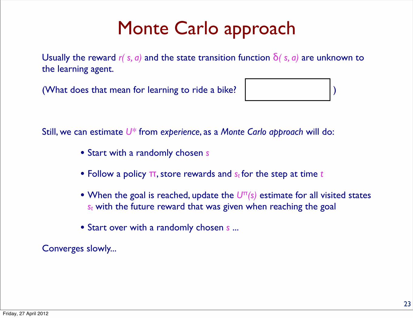
Monte Carlo approachUsually the reward r( s, a) and the state transition function δ( s, a) are unknown to the learning agent.
23Friday, 27 April 2012

Monte Carlo approachUsually the reward r( s, a) and the state transition function δ( s, a) are unknown to the learning agent.
(What does that mean for learning to ride a bike? )
23Friday, 27 April 2012

Monte Carlo approachUsually the reward r( s, a) and the state transition function δ( s, a) are unknown to the learning agent.
(What does that mean for learning to ride a bike? )
23Friday, 27 April 2012

Monte Carlo approachUsually the reward r( s, a) and the state transition function δ( s, a) are unknown to the learning agent.
(What does that mean for learning to ride a bike? )
Still, we can estimate U* from experience, as a Monte Carlo approach will do:
• Start with a randomly chosen s
• Follow a policy π, store rewards and st for the step at time t
•When the goal is reached, update the Uπ(s) estimate for all visited states st with the future reward that was given when reaching the goal
• Start over with a randomly chosen s ...
23Friday, 27 April 2012
Monte Carlo approachUsually the reward r( s, a) and the state transition function δ( s, a) are unknown to the learning agent.
(What does that mean for learning to ride a bike? )
Still, we can estimate U* from experience, as a Monte Carlo approach will do:
• Start with a randomly chosen s
• Follow a policy π, store rewards and st for the step at time t
•When the goal is reached, update the Uπ(s) estimate for all visited states st with the future reward that was given when reaching the goal
• Start over with a randomly chosen s ...
Converges slowly...
23Friday, 27 April 2012

Temporal Difference learning
24Friday, 27 April 2012
Temporal Difference learning
Temporal Difference learning ...
24Friday, 27 April 2012

Temporal Difference learning
Temporal Difference learning ...
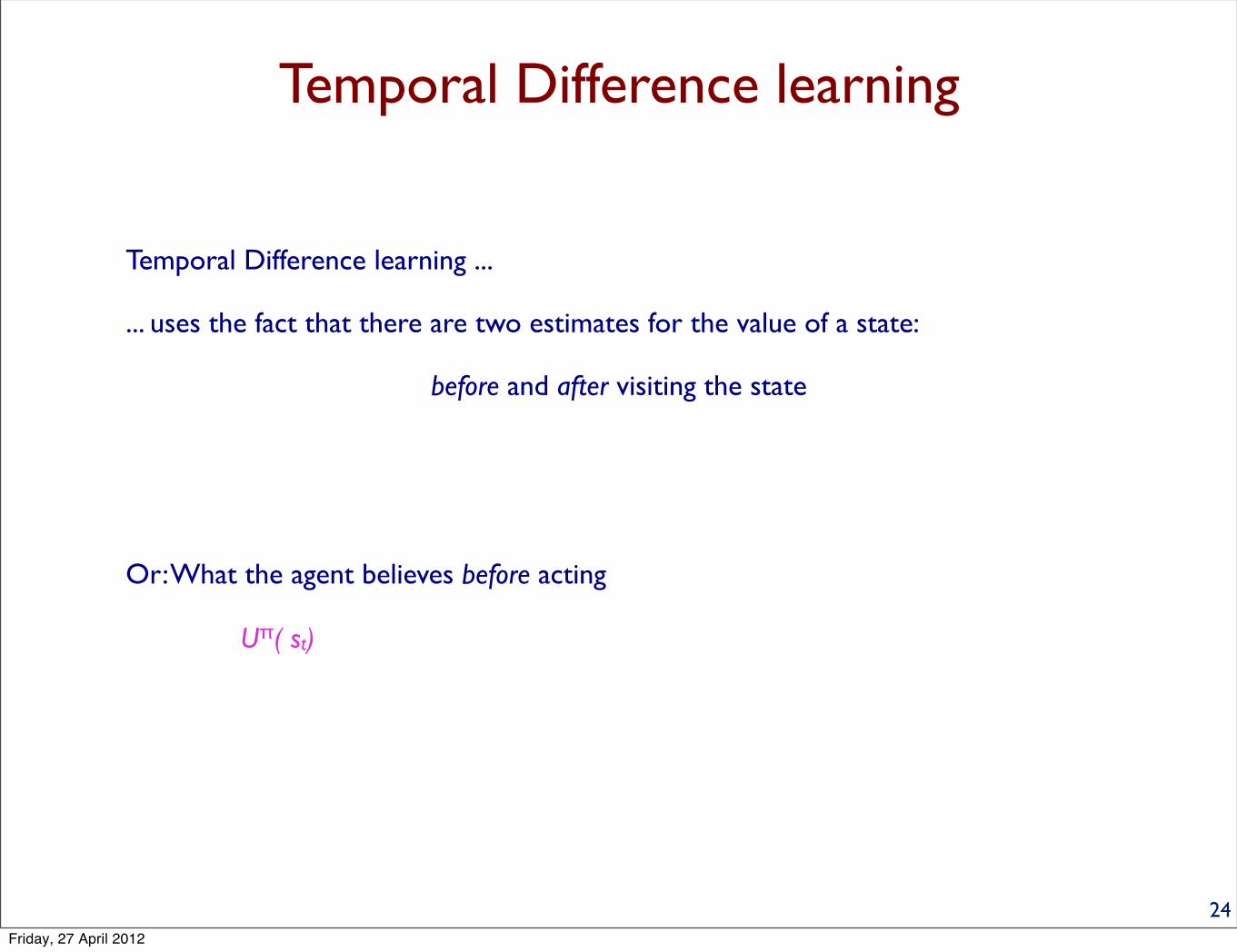
... uses the fact that there are two estimates for the value of a state:
24Friday, 27 April 2012
Temporal Difference learning
Temporal Difference learning ...
... uses the fact that there are two estimates for the value of a state:
before and after visiting the state
24Friday, 27 April 2012

Temporal Difference learning
Temporal Difference learning ...
... uses the fact that there are two estimates for the value of a state:
before and after visiting the state
24Friday, 27 April 2012

Temporal Difference learning
Temporal Difference learning ...
... uses the fact that there are two estimates for the value of a state:
before and after visiting the state
24Friday, 27 April 2012
Temporal Difference learning
Temporal Difference learning ...
... uses the fact that there are two estimates for the value of a state:
before and after visiting the state
Or: What the agent believes before acting
Uπ( st)
24Friday, 27 April 2012

Temporal Difference learning
Temporal Difference learning ...
... uses the fact that there are two estimates for the value of a state:
before and after visiting the state
Or: What the agent believes before acting
Uπ( st)
and after acting
rt+1 + γ · Uπ( st+1)
24Friday, 27 April 2012

Applying the estimates
25Friday, 27 April 2012

Applying the estimatesThe second estimate in the Temporal Difference learning approach is obviously “better”, ...
25Friday, 27 April 2012
Applying the estimatesThe second estimate in the Temporal Difference learning approach is obviously “better”, ...
... hence, we update the overall approximation of a state’s value towards the more accurate estimate
25Friday, 27 April 2012

Applying the estimatesThe second estimate in the Temporal Difference learning approach is obviously “better”, ...
... hence, we update the overall approximation of a state’s value towards the more accurate estimate
Uπ( st) ⟵ Uπ( st) + α[ rt+1 + γ·Uπ ( st+1) - Uπ( st)]
25Friday, 27 April 2012

Applying the estimatesThe second estimate in the Temporal Difference learning approach is obviously “better”, ...
... hence, we update the overall approximation of a state’s value towards the more accurate estimate
Uπ( st) ⟵ Uπ( st) + α[ rt+1 + γ·Uπ ( st+1) - Uπ( st)]
Which gives us a measure of the “surprise” or “disappointment” for the outcome of an action.
Converges significantly faster than the pure Monte Carlo approach.
25Friday, 27 April 2012

Q-learning
26Friday, 27 April 2012

Q-learningProblem:
26Friday, 27 April 2012

Q-learningProblem:
even if U is appropriately estimated, it is not possible to compute π, as the agent has no knowledge about δ and r, i.e., it needs to learn also that.
26Friday, 27 April 2012

Q-learningProblem:
even if U is appropriately estimated, it is not possible to compute π, as the agent has no knowledge about δ and r, i.e., it needs to learn also that.
Solution (trick): Estimate Q( s, a) instead of U(s):
26Friday, 27 April 2012

Q-learningProblem:
even if U is appropriately estimated, it is not possible to compute π, as the agent has no knowledge about δ and r, i.e., it needs to learn also that.
Solution (trick): Estimate Q( s, a) instead of U(s):
Q( s, a): Expected total reward when choosing a in s
π(s) = argmax Q( s, a)
26Friday, 27 April 2012

Q-learningProblem:
even if U is appropriately estimated, it is not possible to compute π, as the agent has no knowledge about δ and r, i.e., it needs to learn also that.
Solution (trick): Estimate Q( s, a) instead of U(s):
Q( s, a): Expected total reward when choosing a in s
π(s) = argmax Q( s, a)a
U*( s) = max Q*( s, a)
26Friday, 27 April 2012

Q-learningProblem:
even if U is appropriately estimated, it is not possible to compute π, as the agent has no knowledge about δ and r, i.e., it needs to learn also that.
Solution (trick): Estimate Q( s, a) instead of U(s):
Q( s, a): Expected total reward when choosing a in s
π(s) = argmax Q( s, a)a
U*( s) = max Q*( s, a) a
26Friday, 27 April 2012
Learning Q
27Friday, 27 April 2012

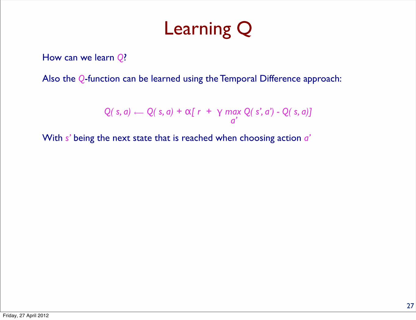
Learning QHow can we learn Q?
27Friday, 27 April 2012

Learning QHow can we learn Q?
Also the Q-function can be learned using the Temporal Difference approach:
27Friday, 27 April 2012

Learning QHow can we learn Q?
Also the Q-function can be learned using the Temporal Difference approach:
Q( s, a) ⟵ Q( s, a) + α[ r + γ max Q( s’, a’) - Q( s, a)]
27Friday, 27 April 2012

Learning QHow can we learn Q?
Also the Q-function can be learned using the Temporal Difference approach:
Q( s, a) ⟵ Q( s, a) + α[ r + γ max Q( s’, a’) - Q( s, a)] a’
27Friday, 27 April 2012
Learning QHow can we learn Q?
Also the Q-function can be learned using the Temporal Difference approach:
Q( s, a) ⟵ Q( s, a) + α[ r + γ max Q( s’, a’) - Q( s, a)] a’
With s’ being the next state that is reached when choosing action a’
27Friday, 27 April 2012

Learning QHow can we learn Q?
Also the Q-function can be learned using the Temporal Difference approach:
Q( s, a) ⟵ Q( s, a) + α[ r + γ max Q( s’, a’) - Q( s, a)] a’
With s’ being the next state that is reached when choosing action a’
Again, a problem: the max operator requires obviously a search through all possible actions that can be taken in the next step...
27Friday, 27 April 2012

SARSA-learning
28Friday, 27 April 2012
SARSA-learning
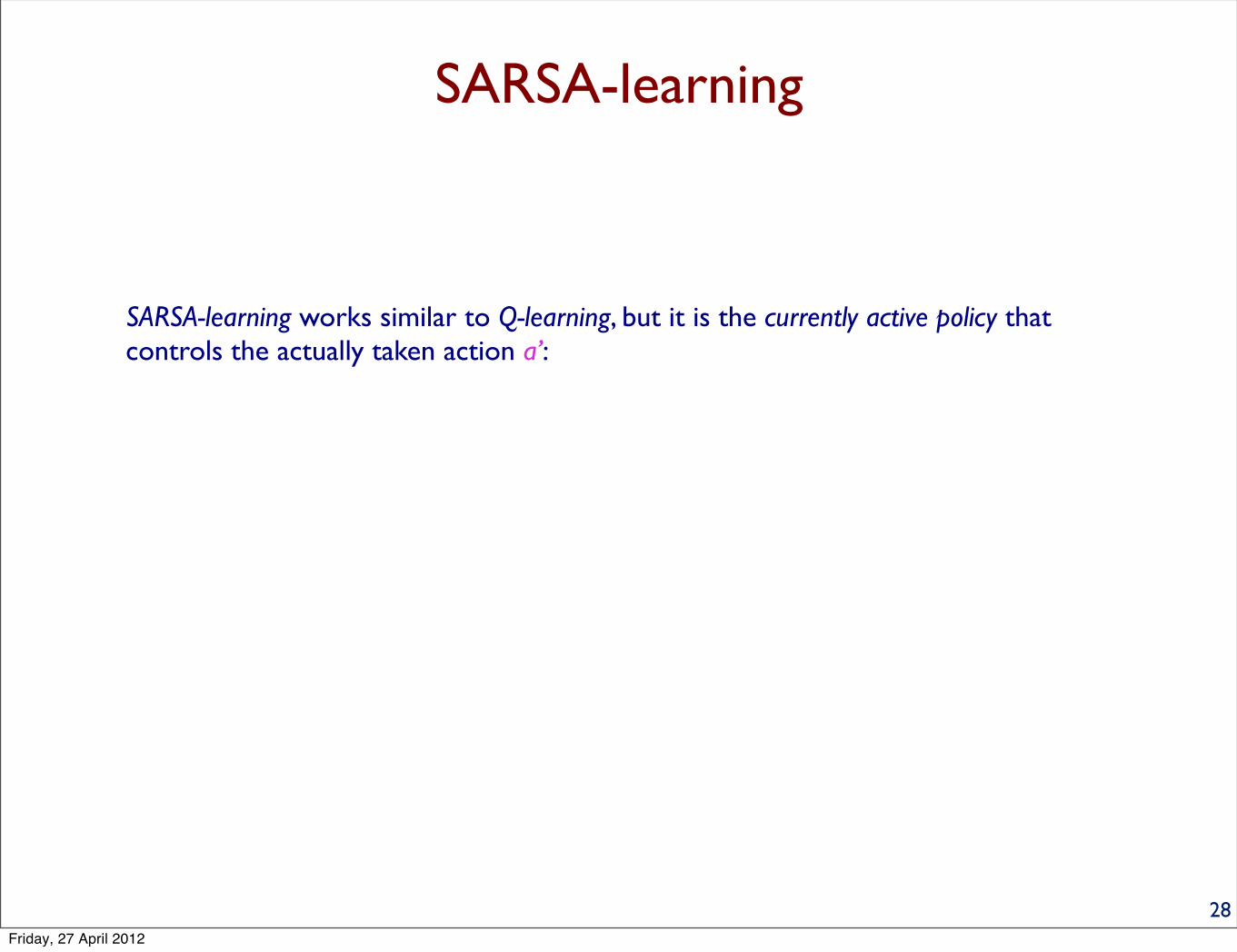
SARSA-learning works similar to Q-learning, but it is the currently active policy that controls the actually taken action a’:
28Friday, 27 April 2012

SARSA-learning
SARSA-learning works similar to Q-learning, but it is the currently active policy that controls the actually taken action a’:
Q( s, a) ⟵ Q( s, a) + α[ r + γ Q( s’, a’) - Q( s, a)]
28Friday, 27 April 2012

SARSA-learning
SARSA-learning works similar to Q-learning, but it is the currently active policy that controls the actually taken action a’:
Q( s, a) ⟵ Q( s, a) + α[ r + γ Q( s’, a’) - Q( s, a)]
28Friday, 27 April 2012

SARSA-learning
SARSA-learning works similar to Q-learning, but it is the currently active policy that controls the actually taken action a’:
Q( s, a) ⟵ Q( s, a) + α[ r + γ Q( s’, a’) - Q( s, a)]
Got its name from the “experience tuples” having the form
State-Action-Reward-State-Action
< s, a, r, s’, a’ >
28Friday, 27 April 2012
Outline• Reinforcement learning (chapter 21, with some references to 17)
• Problem definition
• Learning situation
• Roll of the reward
• Simplified assumptions
• Central concepts and terms
• Known environment
• Bellman’s equation
• Approaches to solutions
• Unknown environment
• Monte-Carlo method
• Temporal-Difference learning
• Q-Learning
• Sarsa-Learning
• Improvements
• The usefulness of making mistakes
• Eligibility Trace
29Friday, 27 April 2012

Improvements and adaptations
What can we do, when ...
• ... the environment is not fully observable?
• ... there are too many states?
• ... the states are not discrete?
• ... the agent is acting in continuous time?
30Friday, 27 April 2012

Allowing to be wrong sometimes
31Friday, 27 April 2012
Allowing to be wrong sometimes
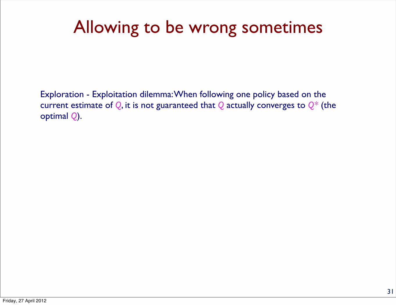
Exploration - Exploitation dilemma: When following one policy based on the current estimate of Q, it is not guaranteed that Q actually converges to Q* (the optimal Q).
31Friday, 27 April 2012

Allowing to be wrong sometimes
Exploration - Exploitation dilemma: When following one policy based on the current estimate of Q, it is not guaranteed that Q actually converges to Q* (the optimal Q).
A simple solution: Use a policy that has a certain probability of “being wrong” once in a while, to explore better.
• ε-greedy: Will sometimes (with probability ε) pick a random action instead of the one that looks best (greedy)
• Softmax: Weighs the probability for choosing different actions according to how “good” they appear to be.
31Friday, 27 April 2012

ε-greedy Q-learning
32Friday, 27 April 2012

ε-greedy Q-learning
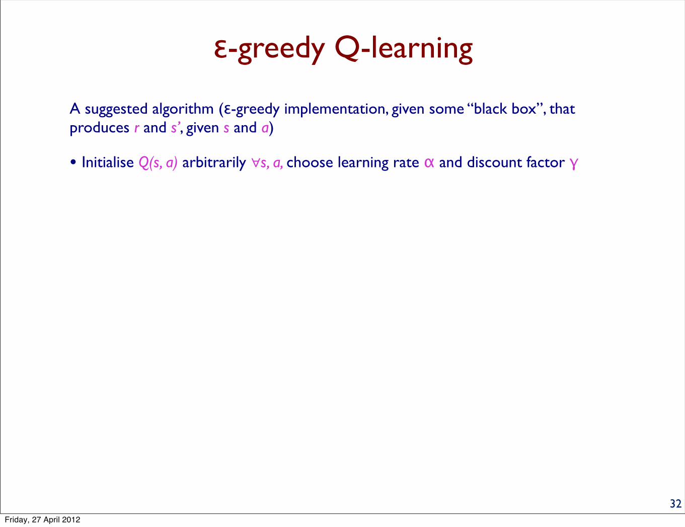
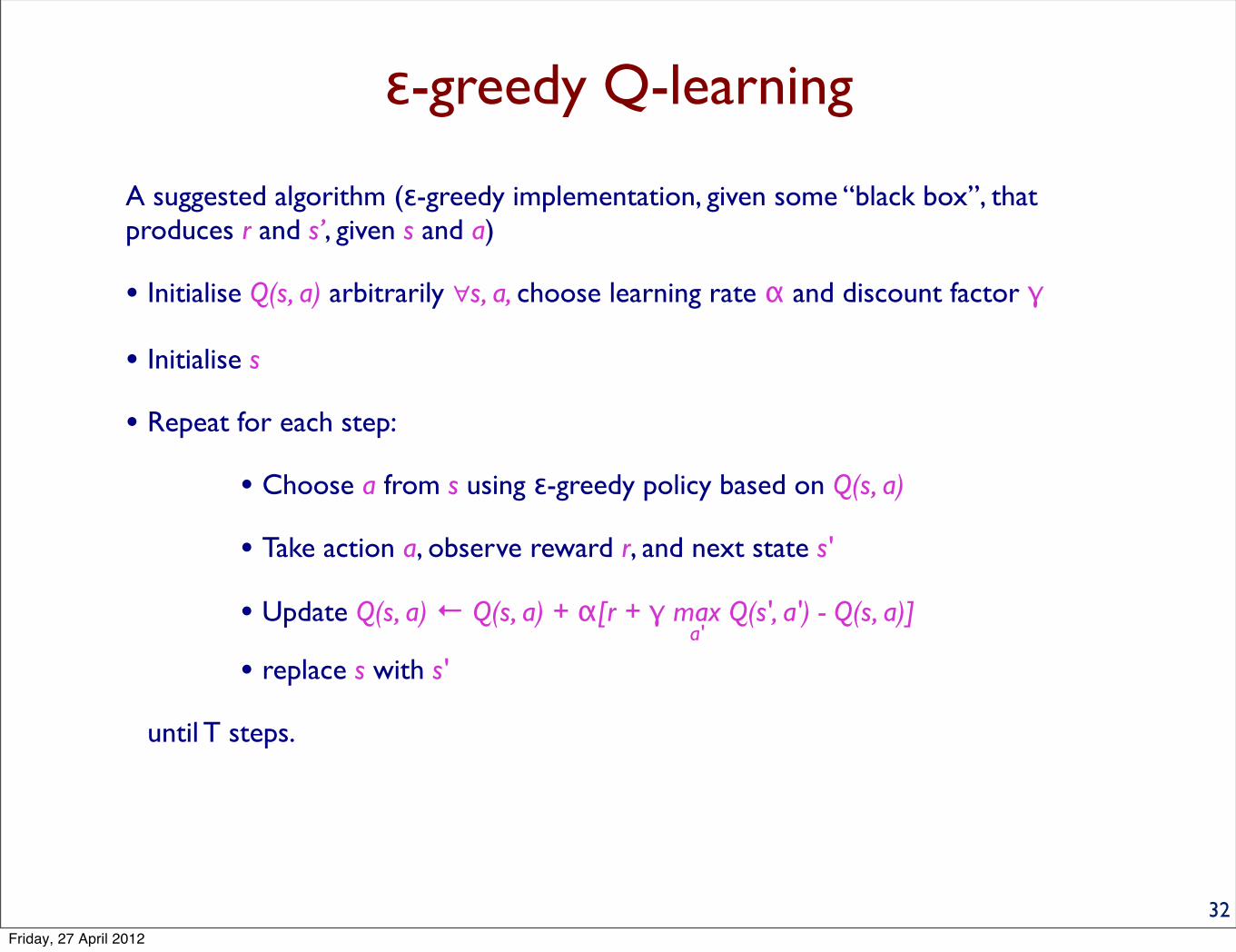
A suggested algorithm (ε-greedy implementation, given some “black box”, that produces r and s’, given s and a)
32Friday, 27 April 2012
ε-greedy Q-learning
A suggested algorithm (ε-greedy implementation, given some “black box”, that produces r and s’, given s and a)
• Initialise Q(s, a) arbitrarily ∀s, a, choose learning rate α and discount factor γ
32Friday, 27 April 2012

ε-greedy Q-learning
A suggested algorithm (ε-greedy implementation, given some “black box”, that produces r and s’, given s and a)
• Initialise Q(s, a) arbitrarily ∀s, a, choose learning rate α and discount factor γ
• Initialise s
32Friday, 27 April 2012

ε-greedy Q-learning
A suggested algorithm (ε-greedy implementation, given some “black box”, that produces r and s’, given s and a)
• Initialise Q(s, a) arbitrarily ∀s, a, choose learning rate α and discount factor γ
• Initialise s
• Repeat for each step:
• Choose a from s using ε-greedy policy based on Q(s, a)
• Take action a, observe reward r, and next state s'
• Update Q(s, a) ← Q(s, a) + α[r + γ max Q(s', a') - Q(s, a)] a'
• replace s with s'
until T steps.
32Friday, 27 April 2012

Speeding up the process
Idea: the Time Difference (TD) updates can be used to improve the estimation also of states where the agent has already been earlier.
∀s, a : Q( s, a) ⟵ Q( s, a) + α[ rt+1 + γ Q( st+1, at+1) - Q( st, at)] · e
With e the eligibility trace, telling how long ago the agent visited s and chose action a
Often called TD( λ), with λ being the time constant that describes the “annealing rate” of the trace.
33Friday, 27 April 2012

Application examples
• Game playing.
• A. Samuel’s checkers program (1959). Remarkable: did not use any rewards... but was managed to converge anyhow...
• G. Tesauro’s backgammon program from 1992, first introduced as Neurogammon, with a neural network representation of Q(s, a). Required an expert for tedious training ;-) The newer version TD-gammon learned from self-play and rewards at the end of the game according to generalised TD-learning. Played quite well after two weeks of computing time ...
• Robotics
• Classic example: the inverse pendulum (cart-pole). Two actions: jerk right or jerk left (bang-bang control). First learning algorithm to this problem applied in 1968 (Michie and Chambers), using a real cart!
• More recently: Pancake flipping ;-)
34Friday, 27 April 2012

Flipping ... a piece of (pan)cake?
35
Video from programming-by-demonstration.org(Dr. Sylvain Calinon & Dr. Petar Kormushev)
Friday, 27 April 2012

Homework for Machine Learning
• Homework 3 is related to machine learning, announced on the course page
• Choose between 3a, 3b, 3c (or do several), but only one (the best) will contribute in the end as homework 3
• 3c is in the area of today’s lecture (slides will be provided after the lecture ;-)
• The task: get a little two-legged agent (“robot”) to learn to “walk”
• Some programming effort is involved (instructions provided)
• Main idea is to explore different reinforcement learning approaches and compare their effect on the agent’s success (or failure...) and report on the experience
• A series of images for “animation” of the agent is provided
• Support methods for the “animation” of the agent’s walk are provided in Matlab and Python (transferring to Java should also be easily possible, the Matlab code is less than 30 lines long)
36Friday, 27 April 2012
Homework for Machine Learning cont’d
• Seemingly “simple” task - just doing it gives a grade 3 at maximum.
• BUT: the important part of this task is the INTERPRETATION and DISCUSSION of results, which should be done in a thoroughly prepared and written REPORT. Please make sure you have read the instructions carefully before starting the work!
• Deadline for handing in: May 10, 2012.
37Friday, 27 April 2012
![Wumpus World 1 Wumpus and 1 pile of gold in a pit-filled cave Starts in [1,1] facing right - Random cave Percepts: [smell, breeze, gold, bump, scream]](https://static.fdocuments.us/doc/165x107/56649d4a5503460f94a269d4/wumpus-world-1-wumpus-and-1-pile-of-gold-in-a-pit-filled-cave-starts-in-11.jpg)