Reinforcement learningA comparison o�earning agents in environments with largediscrete state spacesBachelor’s thesis in Computer Science

JOHAN ANDERSSONEMIL KRISTIANSSONJOAKIM PERSSONADAM SANDBERG ERIKSSONDANIEL TOOMJOPPE WIDSTAM

Department of Computer Science and EngineeringCHALMERS UNIVERSITY OF TECHNOLOGY

4102nedewS,grobetoG

BACHELOR’S THESIS IN COMPUTER SCIENCE

Reinforcement learning

A comparison of learning agents in environments with large discrete state spaces

JOHAN ANDERSSONEMIL KRISTIANSSON

JOAKIM PERSSONADAM SANDBERG ERIKSSON

DANIEL TOOMJOPPE WIDSTAM

Department of Computer Science and EngineeringCHALMERS UNIVERSITY OF TECHNOLOGY

Goteborg, Sweden 2014

The Author grants to Chalmers University of Technology and University of Gothen-burg the non-exclusive right to publish the Work electronically and in a non-commercial purpose make it accessible on the Internet.

The Author warrants that he/she is the author to the Work, and warrants that theWork does not contain text, pictures or other material that violates copyright law.

The Author shall, when transferring the rights of the Work to a third party (forexample a publisher or a company), acknowledge the third party about this agree-ment. If the Author has signed a copyright agreement with a third party regardingthe Work, the Author warrants hereby that he/she has obtained any necessarypermission from this third party to let Chalmers University of Technology andUniversity of Gothenburg store the Work electronically and make it accessible onthe Internet.

Reinforcement learningA comparison of learning agents in environments with large discrete state spacesJOHAN ANDERSSONEMIL KRISTIANSSONJOAKIM PERSSONADAM SANDBERG ERIKSSONDANIEL TOOMJOPPE WIDSTAM

c© JOHAN ANDERSSON, EMIL KRISTIANSSON, JOAKIM PERSSON, ADAMSANDBERG ERIKSSON, DANIEL TOOM, JOPPE WIDSTAM, 2014

Examiner: JAN SKANSHOLM

Bachelor’s thesis 2014:05ISSN 1654-4676Department of Computer Science and EngineeringChalmers University of TechnologySE-412 96 GoteborgSwedenTelephone: +46 (0)31-772 1000

Chalmers ReproserviceGoteborg, Sweden 2014

Abstract

For some real-world optimization problems where the best behavior is sought, it isinfeasible to search for a solution by making a model of the problem and performingcalculations on it. When this is the case, good solutions can sometimes be foundby trial and error. Reinforcement learning is a way of finding optimal behaviorby systematic trial and error. This thesis aims to compare different reinforcementlearning techniques and evaluate them. Model-based interval estimation (MBIE)and Explicit Explore or Exploit using dynamic bayesian networks (DBN-E3) aretwo algorithms that are evaluated. To evaluate the techniques, learning agentswere constructed using the algorithms and then simulated in the environment In-vasive Species from the Reinforcement Learning Competition. The results of thestudy show that an optimized version of DBN-E3 is better than MBIE at findingan optimal or near optimal behavior policy in Invasive Species for a selection ofenvironment parameters. Using a factored model like a DBN shows certain advan-tages operating in Invasive Species, which is a factored environment. For exampleit achieves a near optimal policy within fewer episodes than MBIE.

Keywords: Reinforcement learning, Artificial intelligence, MBIE, DBN-E3, Inva-sive Species, Learning algorithms

i

Sammanfattning

For vissa verklighetsbaserade optimeringsproblem dar det galler att finna ett bastabeteende ar det orimligt soka efter det optimala beteendet genom att skapa enmodell av problemet och sedan utfora berakningar pa den. Nar sa ar fallet, kanman hitta bra losningar genom trial and error. Reinforcement learning ar ett sattatt hitta optimalt beteende genom att systematisk prova sig fram. Detta kandi-datarbete har som mal att jamfora olika inlarningstekniker och utvardera dessa.Model-based interval estimation (MBIE) och Explicit Explore or Exploit med dy-namiska bayesnat (DBN-E3) ar tva sjalvlarande algoritmer som har utvarderas.For att utvardera de olika teknikerna implementerades agenter som anvande al-goritmerna, och dessa testkordes sedan i miljon Invasive Species fran tavlingenReinforcement Learning Competition. DBN-E3 ar battre an MBIE pa att hittaen optimal eller nara optimal policy i Invasive Species med valda parametrar. Attanvanda en faktoriserad modell, sa som DBN-E3 visar pa tydliga fordelar i fakto-riserade miljoer, som i till exempel Invasive Species. Ett exempel pa detta ar attden nar en nastan optimal policy pa farre episoder an MBIE.

ii

Contents

Abstract i

Sammanfattning ii

1 Introduction 11.1 Purpose and problem statement . . . . . . . . . . . . . . . . . . . . . 1

2 Technical background 32.1 Reinforcement learning . . . . . . . . . . . . . . . . . . . . . . . . . . 3

2.1.1 Episodic and non-episodic problems . . . . . . . . . . . . . . 42.1.2 Continuous and discrete problems . . . . . . . . . . . . . . . 4

2.2 Markov decision process . . . . . . . . . . . . . . . . . . . . . . . . . 42.2.1 Utility . . . . . . . . . . . . . . . . . . . . . . . . . . . . . . . 52.2.2 Markov property . . . . . . . . . . . . . . . . . . . . . . . . . 52.2.3 Representations . . . . . . . . . . . . . . . . . . . . . . . . . . 5

2.3 Basic algorithms for solving MDPs . . . . . . . . . . . . . . . . . . . 62.3.1 Value functions . . . . . . . . . . . . . . . . . . . . . . . . . . 62.3.2 Policy iteration . . . . . . . . . . . . . . . . . . . . . . . . . . 72.3.3 Value iteration . . . . . . . . . . . . . . . . . . . . . . . . . . 7

2.4 Dynamic bayesian networks . . . . . . . . . . . . . . . . . . . . . . . 8

3 Environment and algorithms 103.1 Environment specification, Invasive Species . . . . . . . . . . . . . . 103.2 Model-based interval estimation . . . . . . . . . . . . . . . . . . . . . 11

3.2.1 Value iteration with confidence intervals . . . . . . . . . . . . 113.2.2 Optimistic estimations of transition probabilities . . . . . . . 123.2.3 ComputeP . . . . . . . . . . . . . . . . . . . . . . . . . . . . 123.2.4 Optimizations based on Good-Turing estimations . . . . . . . 13

3.3 E3 in factored Markov decision processes . . . . . . . . . . . . . . . 133.3.1 The E3 algorithm . . . . . . . . . . . . . . . . . . . . . . . . 133.3.2 Factored additions to E3 . . . . . . . . . . . . . . . . . . . . 14

4 Method 164.1 Algorithm implementation . . . . . . . . . . . . . . . . . . . . . . . . 16

4.1.1 Implementation choices and extensions for MBIE . . . . . . . 164.1.2 Implementation choices and extensions for DBN-E3 . . . . . 174.1.3 GridWorld . . . . . . . . . . . . . . . . . . . . . . . . . . . . 184.1.4 Network simulator . . . . . . . . . . . . . . . . . . . . . . . . 18

4.2 Test specification . . . . . . . . . . . . . . . . . . . . . . . . . . . . . 184.3 RL-Glue . . . . . . . . . . . . . . . . . . . . . . . . . . . . . . . . . . 20

5 Results 22

6 Discussion 246.1 Evaluation of the agents . . . . . . . . . . . . . . . . . . . . . . . . . 24

6.1.1 E3 in factored MDPs . . . . . . . . . . . . . . . . . . . . . . 246.1.2 MBIE . . . . . . . . . . . . . . . . . . . . . . . . . . . . . . . 256.1.3 DBN-E3 vs MBIE . . . . . . . . . . . . . . . . . . . . . . . . 25

6.2 Potential factors impacting the results . . . . . . . . . . . . . . . . . 266.2.1 Impact of using one environment . . . . . . . . . . . . . . . . 266.2.2 Implementation of algorithms . . . . . . . . . . . . . . . . . . 276.2.3 Testing methodology . . . . . . . . . . . . . . . . . . . . . . . 27

iii

6.3 Using models for simulating real world problems . . . . . . . . . . . 276.4 Further work . . . . . . . . . . . . . . . . . . . . . . . . . . . . . . . 28

6.4.1 Testing algorithms with more environments . . . . . . . . . . 286.4.2 Planning algorithm for DBN-E3 in factored MDPs . . . . . . 286.4.3 Improvements to MBIE . . . . . . . . . . . . . . . . . . . . . 286.4.4 Extend MBIE to utilize a factored representation . . . . . . . 29

References 29

iv

Chapter 1

Introduction

Reinforcement learning, a subfield of artificial intelligence, is the study of algo-rithms that learn how to choose the best actions depending on the situation. Ina reinforcement learning problem the algorithm is not told which actions give thebest results, but instead it has to interact with the environment to learn when andwhere to take a certain action. When the agent has learned about each situationor state of the environment, it will arrive at an optimal sequence of actions (Bartoand Sutton 1998).

Reinforcement learning can be exemplified by how a newborn animal learns howto stand up. There is no tutor to teach it, so instead it tries various combinationsof movements, while remembering which of them lead to success and which of themlead to failure. Probably, at first, most of its attempted movement patterns willlead to it falling down — a negative result, making the animal less likely to trythose patterns again. After a while, the animal finds some combination of musclecontractions that enables it to stand — a positive result, which would make it morelikely to perform those actions again.

In the real world, in order to decide what actions lead to success, one almostalways needs to consider the circumstances, or the state of the environment, inwhich the actions are taken. For instance, a person might be rewarded if theysang beautifully at a concert, but doing the same at the library would probably getthem thrown out. Furthermore, for many real world domains it is common thatthe state space (the set of possible states of the environments in which actions canbe taken) is very large (Guestrin et al. 2003). To continue our example, there areprobably countless places and situations where it is possible to sing. In this case,how does one abstract and find the qualities of the environment that are importantfor deciding on the optimal action?

There are two practical problems connected to reinforcement learning in largestate spaces. First, it is hard to store representations of the states of the environ-ment in the main memory of a computer (Szepesvari 2010). Second, it takes toolong to repeatedly visit all the states to find the best action to take in all of them(Dietterich, Taleghan, and Crowley 2013).

1.1 Purpose and problem statement

This thesis aims to further the knowledge of reinforcement learning or more specifi-cally, algorithms applied to reinforcement learning problems with large state spaces.Reinforcement learning algorithms struggle with environments consisting of largestate spaces due to practical limitations in memory usage and difficulties in estimat-ing the value of actions and states within reasonable processing time. Therefore, weaim to evaluate techniques to circumvent or reduce the impact of these limitations.This is done by implementing algorithms that use these techniques and comparingthe algorithms in an environment with a large state space.

1

Limitations Due to time constraints only two algorithms are tested, which applydifferent techniques. Furthermore, the evaluation of the selected algorithms is donein only one environment covering a certain problem with a large state space.

Simulation environment The environment used is Invasive Species from theReinforcement Learning Competition, described in section 3.1. Depending on theparameters, the problem can have both a large state space and/or a large actionspace. This makes Invasive Species a good choice with the given problem statement.

Agents to be evaluated Two algorithms that are suitable to the purpose andproblem statement, since they apply different techniques for working with largestate spaces, are Explicit Explore or Exploit in dynamic bayesian networks (DBN-E3) and model-based interval estimation (MBIE). They are described in detail inchapter 3.

2

Chapter 2

Technical background

The term artificial intelligence was coined by John McCarthy who described it as“the science and engineering of making intelligent machines” (McCarthy 2007).More specifically, it addresses creating intelligent computer machines or softwarethat can achieve specified goals computationally. These goals can comprise any-thing, e.g. writing poetry, playing complex games such as chess or diagnosingdiseases. Different branches of artificial intelligence include planning, reasoning,pattern recognition and the focus of this thesis: learning from experience. Thischapter gives a more formal description of reinforcement learning and the maintopics and concepts necessary to understand the rest of the report.

2.1 Reinforcement learning

In artificial intelligence, reinforcement learning is the problem of learning fromexperience. A reinforcement learning algorithm uses past experiences and domainknowledge to make intelligent decisions about future actions (Barto and Sutton1998).

ENVIRONMENT

AGENT

Obs

erva

tion

Reward Action

Figure 2.1: The reinforcement learning process

The reinforcement learning problem is modeled as a sequential decision problem,see figure 2.1 for a graphical representation of the process. A learning agent per-

3

forms an action and receives a reward according to some measure of how desirablethe results of the action are. After the action is taken, the state of the environmentchanges and the agent then receives a new observation and the process repeats.The goal of the reinforcement learning agent is to maximize the reward receivedover a certain time period, the horizon, finding a balance between immediate andfuture rewards (Barto and Sutton 1998).

There are several ways of further dividing reinforcement learning problems intoother subcategories. Some examples are the dichotomies episodic/non-episodicproblems, problems with continuous/discrete state spaces, problems with continu-ous/discrete action spaces, problems with one/multiple concurrent agents etc. Inthe text below, the two first of these dichotomies, which are relevant to this thesis,are discussed.

2.1.1 Episodic and non-episodic problems

One can categorize reinforcement learning problems based on whether or not thetime steps are divided into episodes. If they are, the problem is called episodic andotherwise it is called non-episodic. Episodic problems are common in for examplegames, which end when they are won or lost. An episode here corresponds to a fullgame from start to finish. In a non-episodic problem, the interaction between theactor and environment goes on continuously without end (Barto and Sutton 1998).Two examples of non-episodic applications are controlling a robot arm (as well asother robotics problems) and maneuvering a helicopter (Ng et al. 2006).

2.1.2 Continuous and discrete problems

Reinforcement-learning problems can also be categorized by their state spaces.Some problems have a discrete state space whereas for some problems the statespace is continuous. An important difference between the two kinds of problems ishow an agent can treat similar states in the model. In a continuous problem it ismuch easier to classify states located around the same “position” as belonging tothe same group, since the states usually more or less meld together. For example,if the reinforcement learning problem is to control a robot arm whose positionconstitutes the state of the environment, states corresponding to positions in thesame general area are not very different. This means that these states might betreated in the same way or a similar way by an agent. In contrast, consider thediscrete problem of a game of chess, wherein the placement of a pawn in one oftwo adjacent squares could dramatically change the evaluation of the state and theoutcome of the game (Barto and Sutton 1998).

2.2 Markov decision process

Within reinforcement learning, the concept of Markov decision processes (MDP)is central. An MDP is a way to model an environment where state changes in itare dependent on both random chance and the actions of an agent. An MDP isdefined by the quadruple (S,A, P (·, ·, ·), R(·, ·)) (Altman 2002):

Definition 2.1. MDP

S A set of states that the environment can be in.

A A set of actions that are allowed in the MDP.

P : S × A × S → [0, 1] A probability distribution over the transitions in theenvironment. This function describes the probability of ending up in a certaintarget state when a certain action is taken from a certain origin state.

R : S × A → R A function for the reward associated with a state transition.In some definitions of MDPs the reward function only depends on the state.

4

MDPs are similar to Markov chains, but there are two differences. First, thereis a concept of rewards in MDPs, which is absent in Markov chains. Second, in aMarkov chain, the only thing that affects the probabilities of transitioning to otherstates is the current state, whereas in an MPD both the current state and the actiontaken in that state are needed to know the probability distribution connected withthe next state (Altman 2002).

If there are only a few states s′ for which P (s, a, s′) > 0, the MDP is calleda sparse MDP. That is to say, when an agent performs a certain action, a, in acertain state, s, the environment can only end up in a small fraction out of thetotal number of states (Dietterich, Taleghan, and Crowley 2013).

2.2.1 Utility

The concept of utility is used as a measurement of how well an agent performs overtime. In the simplest case, the utility is just the sum of all rewards received inan episode. See equation (2.1), where T is the length of an episode and rk is theexpected reward at time step k.

U0 = r0 + r1 + · · ·+ rT−1 =

T−1∑k=0

rk (2.1)

However, in a non-episodic environment, the interaction between the environ-ment and the agent can go on forever. Here the concept of a discount factor, γ, isessential. This parameter is a value between 0 and 1 which describes how fast thevalue of expected future rewards decays as one looks further into the future (Bartoand Sutton 1998). Thus, the utility can be expressed as in equation (2.2) in thecase that discounting is used.

Ut = rt+1 + γrt+2 + γ2rt+3 · · · =∞∑k=0

γkrt+k+1 (2.2)

2.2.2 Markov property

A defining characteristic of an MDP is the Markov property—that, given the cur-rent state of the environment, one cannot gain any more information about itsfuture behavior by also considering the previous actions and states it has beenin. Equation (2.3) defines the Markov property: the probability of state st+1 onlydepends on the previous state st and action at.

Pr(st+1|st, at, . . . , s1, a1) = Pr(st+1|st, at) = P (st, at, st+1) (2.3)

This can be compared to the state of a chess game, where the positions ofthe pieces at any time completely summarizes everything relevant about what hashappened previously in the game. That is, no more information about previousmoves or states of the board is needed to decide how to play or predict the futureoutcome of the game (disregarding psychological factors). A chess MDP that usesa chess board as its state representation could thus be an example of an MDP withthe Markov property (Altman 2002).

2.2.3 Representations

Two ways to represent an MDP are extensional and factored representation. De-pending on what problem domain is used, it can be advantageous to use a factoredrepresentation due to computational considerations(Boutilier, Dean, and Hanks1999).

5

Extensional representation The most straightforward way to model an MDPis called extensional representation, where the set of states and actions are enu-merated directly. It is also commonly referred to as an explicit representation andthis is the definition we have used so far in the report when discussing the abstractview of an MDP (Boutilier, Dean, and Hanks 1999).

Factored representation A factored representation of the states of an MDPoften results in a more compact way of describing the set of states. Certain prop-erties or features of the states are used to factor the state space into different sets.Which properties or features are used is chosen by the algorithm designer, to fitthe environment. Formally a state s is in a state space S = S1 × · · · × Sk of kfactors, with the state at time t being st = (st(1), . . . , st(k)).

When the MDP is factored, it enables factored representations of states, ac-tions and other components of the MDP as well. When using a factored actionrepresentation, an action can be taken based on specific state features instead ofon the whole state. If the individual actions affect relativity few features or ifthe effects contain regularities then using a factored representation can result incompact representations of actions (Boutilier, Dean, and Hanks 1999).

2.3 Basic algorithms for solving MDPs

A policy π is a function from a state s to an action a that operates in the contextof a Markov decision process, i.e. π : S → A. A policy is thus a description ofhow to act in each state of an MDP. An arbitrary policy is denoted by π and theoptimal policy (the policy with the maximal utility in the MDP) is denoted by π∗.The rest of this section describes some basic algorithms for solving an MDP, thatis to say, finding an optimal policy for it (Barto and Sutton 1998).

2.3.1 Value functions

To solve an MDP, most algorithms use an estimation of values of states or statesand actions. Two value functions are usually defined, the state-value functionV : S → R and the state-action-value function Q : S×A→ R. As the names imply,V signifies how good a state is, while Q signifies how good an action in a state is.The state-value function, V π(s), returns the expected value when starting in state sand following policy π thereafter. The state-action-value function, Qπ(s, a), returnsthe expected value when starting in state s and taking action a and thereafterfollowing policy π. The value functions for the optimal policy, the policy thatmaximizes the utility, are denoted by V ∗(s) and Q∗(s, a) (Barto and Sutton 1998).

Equations (2.4) and (2.5) show the state-value function V and the state-action-value function Q defined in terms of utility (section 2.2.1). The future states, st,are stochastically distributed according to the transition probabilities of the MDPand the policy π (see section 2.2).

V πt (s) = E {Ut| st = s} (2.4)

Qπt (s, a) = E {Ut| st = s, at = a} (2.5)

Both V π and Qπ can be estimated from experience. This can be done bymaintaining the average of the rewards that have followed each state when followingthe policy π. When the number of times the state has been encountered goes toinfinity, the average over these histories of rewards converges to the true values ofthe value function (Barto and Sutton 1998).

6

Using dynamic programming to find V and Q Another way to find valuefunctions is to use dynamic programming techniques. Dynamic programming is away of dividing a problem into subproblems that can be solved independently. Ifthe result of a particular subproblem is needed again, it can be looked up from atable (Bellman 1957). Examples of dynamic programming algorithms are policyiteration and value iteration, which are discussed in sections 2.3.2 and 2.3.3. Thesealgorithms are often the basis for more advanced algorithms, among them the onesdescribed in chapter 3.

2.3.2 Policy iteration

Policy iteration is a method for solving an MPD that will converge to an optimalpolicy and the true value function in a finite number of iterations if the process is afinite MDP. The algorithm consists of three steps: initialization, policy evaluationand policy improvement (Barto and Sutton 1998).

InitializationStart with an arbitrary policy π and arbitrary value function V0.

Policy evaluationCompute an updated value function, V , for the policy π in the MDP by usingthe update rule (2.6) until V converges. Convergence means that |Vk+1(s)−Vk(s)| ≤ ε,∀s, where ε is chosen as a small value. In the update rule, π(s, a)is the probability of taking action a in state s using policy π.

Vk+1(s) =∑a

π(s, a)∑s′

P (s, a, s′) [R(s, a) + γVk(s′)] (2.6)

Policy improvementImprove the policy by making it greedy with regard to V , equation (2.7)1.This means that the policy will describe the action in each state that maxi-mizes the expected V -value of the following state.

πk+1(s) = arg maxa

∑s′

P (s, a, s′) [R(s, a) + γV (s′)] (2.7)

Repeat evaluation and improvement until π is stable between two iterations.

2.3.3 Value iteration

Value iteration is a simplification of policy iteration where only one step of policyevaluation is performed in each iteration. Value iteration does not compute anactual policy until the value function has converged (Barto and Sutton 1998).Value iteration works as follows:

InitializationStart with an arbitrary value function V0.

Value iterationUpdate the value function for each state using the update rule (2.8).

Vk+1(s) = maxa

∑s′

P (s, a, s′) [R(s, a) + γVk(s′)] (2.8)

1argmaxa f(a) gives the a that maximizes f(a).

7

Repeat value iteration until V converges and set V = Vk. As in policy iteration,by convergence is meant that |Vk+1(s) − Vk(s)| ≤ ε,∀s, where ε is a smallvalue.

Compute the policy using equation (2.9).

π(s) = arg maxa

∑s′

P (s, a, s′) [R(s, a) + γV (s′)] (2.9)

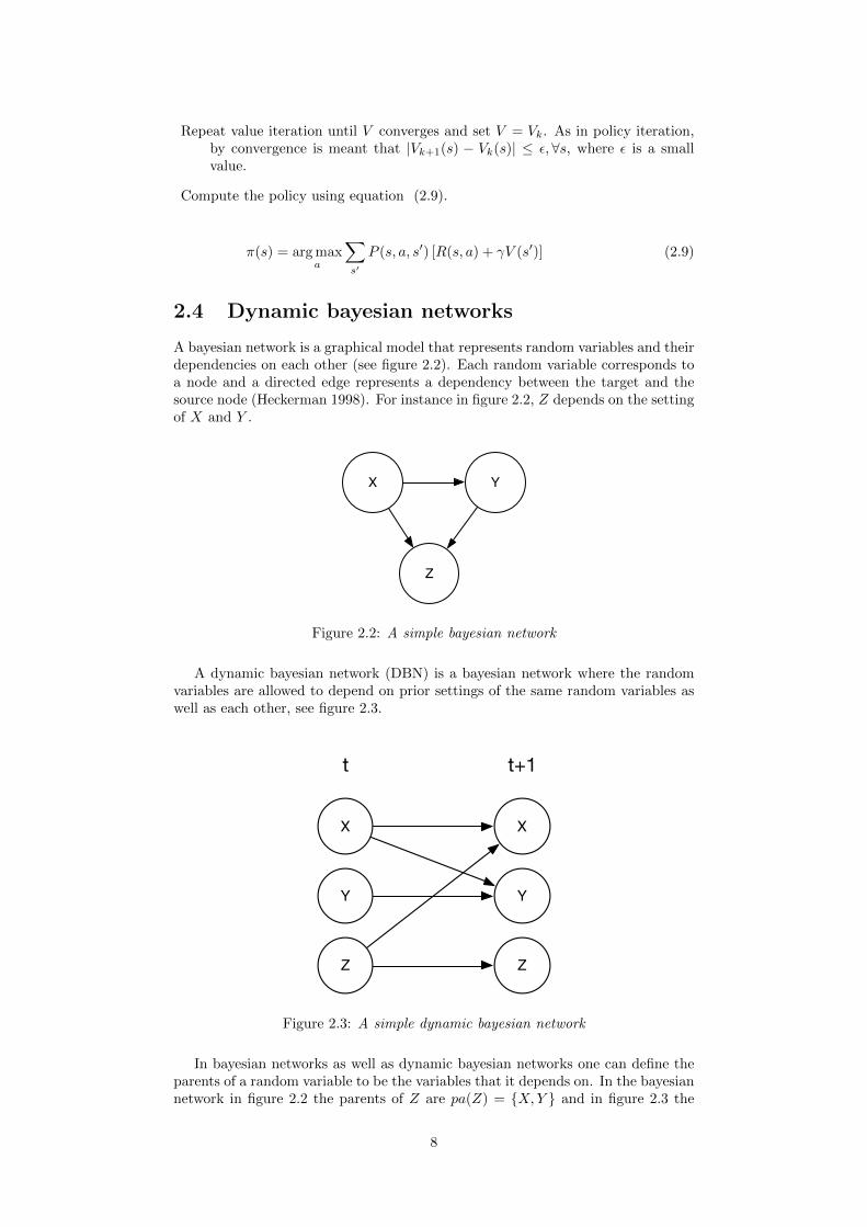
2.4 Dynamic bayesian networks

A bayesian network is a graphical model that represents random variables and theirdependencies on each other (see figure 2.2). Each random variable corresponds toa node and a directed edge represents a dependency between the target and thesource node (Heckerman 1998). For instance in figure 2.2, Z depends on the settingof X and Y .

X

Z

Y

Figure 2.2: A simple bayesian network

A dynamic bayesian network (DBN) is a bayesian network where the randomvariables are allowed to depend on prior settings of the same random variables aswell as each other, see figure 2.3.

X

Y

Z

t

X

Y

Z

t+1

Figure 2.3: A simple dynamic bayesian network

In bayesian networks as well as dynamic bayesian networks one can define theparents of a random variable to be the variables that it depends on. In the bayesiannetwork in figure 2.2 the parents of Z are pa(Z) = {X,Y } and in figure 2.3 the

8

parents of Y are pa(Yt+1) = {Yt, Xt}. A random variable X is not a parent of Y ifthey are independent, i.e. Pr(X,Y ) = Pr(X) Pr(Y ).

States in an MDP can be factored into several state variables representing dif-ferent features of the state. Using this factorization transition probabilities can berepresented by a set of bayesian networks, one network for each possible action.

In each network every state variable, st(i), is a node representing the statevariable at time t, as well as a node, st+1(i), representing the same state variableat time t + 1. If the probability distribution of a certain state variable st+1(i)is affected by the value of another state variable st(j) if action a is taken thenthere is a directed edge from st(j) to st+1(i) in the DBN corresponding to actiona (Guestrin et al. 2003).

9

Chapter 3

Environment and algorithms

This chapter gives a description of the environment and the algorithms that wereused in the experiment described in chapter 4. The environment Invasive Species isa simulation of a river network with invading species, where to goal is to eradicateunwanted species. It is further described in section 3.1.

Two algorithms are covered in this chapter, both of which deal with the prob-lems that arise with large state spaces; however, they differ in the methods theyapply. In the following chapter the general ideas behind the algorithms, as wellas specific details, are presented. The model-based interval estimation algorithm,described in section 3.2, utilizes clever estimations of confidence intervals for thestate-action value functions to improve performance in sparse MDPs. Section 3.3 ison an algorithm that uses dynamic bayesian networks and factored representationsto improve the E3 algorithm to efficiently deal with factored MDPs.

3.1 Environment specification, Invasive Species

When the agents were tested, the Invasive Species environment from the 2014edition of the Reinforcement Learning Competition was used. The environment isa simulation of an invasive species problem, in this case a river network where thegoal of the agent is to eradicate unwanted species while replanting native species.

The environment’s model of the river network has parameters, such as the sizeof the river network and the rate at which plants spread, which can be configuredin order to create different variations of the environment. The size of the rivernetwork is defined by two parameters: the number of reaches and the number ofhabitats per reach. A habitat is the smallest unit of land that is considered inthe problem. A habitat can either be invaded by the tamarix tree, which is anunwanted species, empty or occupied by native species. A reach is a collectionof neighboring habitats. The structure of the river network is defined in terms ofwhich reach is connected to which (Taleghanand, Crowley, and Dietterich 2014).In figure 3.1 a model of a river network is shown.

There are four possible actions (eradicate tamarix trees, plant native trees,eradicate tamarix trees and plant native trees and a wait-and-see action), and theagent chooses one of these actions for each reach and time step. If the agent choosesto eradicate tamarix trees or plant native trees in a reach, all habitats of that reachare targeted by this action. What actions are available to the agent depends onthe state of each reach. It is always possible to choose the wait-and-see action, butthere has to be one or more tamarix-invaded habitats in a reach for the eradicate oreradicate-and-plant actions to be available and there has to be at least one emptyhabitat in a reach for the plant-native-trees action to be available (Taleghanand,Crowley, and Dietterich 2014).

10

Reach

TN

TN

E {}Habitat

No plantE

TNative plant

Tamarix

N

Figure 3.1: A river network, as modeled by the Invasive Species reinforcementlearning environment.

3.2 Model-based interval estimation

Model-based interval estimation (MBIE) is a version of value iteration whose mainfeature is its use of confidence intervals for the state-action values. Optimisticbounds to these confidence intervals are computed, by means of finding an opti-mistic bound for transition probabilities. The optimistic bounds for the transitionprobabilities are then used in standard value iteration to compute state-action val-ues, from which an optimal policy can be found. State values are also computedat this point.

Since the confidence intervals become less wide when the number of data pointsthat they are based on increases, the more times a state-action pair has beenobserved, the less optimistic the bounds for these intervals will be (Dietterich,Taleghan, and Crowley 2013). This has the net result of promoting explorationof state-action pairs as long as the confidence intervals are wide, but as the state-action pairs have been tried more and more times, the agent behaves in a lessexploratory fashion.

3.2.1 Value iteration with confidence intervals

The upper bounds of the confidence intervals for the state-action values are cal-culated as in equation (3.1) and then, using these results, equation (3.2) gives thestate values by taking the best action for each state.

Qupper(s, a) =R(s, a)+

maxP∈CI(P (s,a),δ)

γ∑s′

P (s′|s, a) maxa′

Qupper(s′, a′) (3.1)

Vupper(s) = maxa

Qupper(s, a) (3.2)

11

Section 3.2.3 describes a method, ComputeP , that efficiently calculates themaximization step in equation (3.1) by finding the probability distribution, P ,that maximizes the sum in the equation.

3.2.2 Optimistic estimations of transition probabilities

The first step of the MBIE algorithm is to find optimistic estimations of transitionprobabilities. Equation (3.3) describes, as a set, the confidence interval (CI) usedby MBIE for the probability distribution over destination states when taking actiona in state s. So, the first task of the algorithm is to find the element within this setthat is maximally optimistic, meaning that it gives the best value to (s, a) in thefollowing value-iteration step of the MBIE algorithm. A description of how this isdone in practice is found in section 3.2.3.

In equation (3.3), P is the observed probability distribution (treated as a vector)for destination states from (s, a), N(s, a) is the number of times that the state-action pair (s, a) has been observed, δ is a confidence parameter, ω is the valuegiven by equation (3.4) and ‖x‖1 denotes the L1-norm of the vector x. The L1-normis the sum of the absolute value of all elements of a vector.

CI(P | N(s, a), δ

)={P | ‖P − P‖1 ≤ ω(N(s, a), δ), ‖P‖1 = 1, Pi ≥ 0

}(3.3)

In equation (3.4), ω gives a bound for how much the vector of transition prob-abilities can be changed from the observed values, while remaining within theconfidence interval. In this equation, |S| is the number of states in the MDP andthe other variables have the same meaning as in equation (3.3). For the derivationof this equation, see Strehl and Littman (2008).

ω(N(s, a), δ) =

√2| ln(2|S| − 2)− ln δ|

N(s, a)(3.4)

3.2.3 ComputeP

The method for finding the sought element within the set denoted by equation (3.3)is referred to as ComputeP in this thesis. The fundamental idea of the ComputePmethod is that it starts with the observed transition probabilities P and thenit moves probability mass from “bad” outcomes to “good” outcomes and finallyreturns the resulting probability distribution, P .

Initialization The state transition probability distribution is initialized accord-ing to equation (3.5), which corresponds to the observed probabilities.

P (s′|s, a) := P (s′|s, a) =N(s, a, s′)

N(s, a)(3.5)

In equation (3.5) N(s, a, s′) is the number of times action a has been taken instate s and the agent ended up in state s′.

Moving probability mass The procedure of moving probability mass is doneby first finding the outcome state with the best state-value and observed probabilityless than 1, calling it s. Analogously the outcome with the worst state-value withan observed probability of greater than 0 is found, and this state is called s. If a

12

state-value has not been computed yet for a certain state, it is assumed to havethe maximum possible value.

The probability values P (s|s, a) and P (s|s, a) are then increased or decreasedaccording to equations (3.6) and (3.7).

P (s|s, a) := P (s|s, a)− ξ (3.6)

P (s|s, a) := P (s|s, a) + ξ (3.7)

Since the sum of the probabilities needs to equal one and no single transitionprobability may fall below zero or exceed one, the probability distribution can onlybe modified by at most ξ, as given by equation (3.8), where ∆ω = ω/2. The variable∆ω denotes the total mass that can be moved, without P having a lower chancethan 1− δ of being within the confidence interval for the probability distribution.If ξ is less than ∆ω, new states s and s are found, and probabilities are moved untilmass equal to ∆ω has been moved in total or the probability mass has all beenmoved to an optimal state. The resulting vector, P , is the one that maximizes thesum in equation (3.1).

ξ = min{1− P (s|s, a), P (s|s, a),∆ω} (3.8)

3.2.4 Optimizations based on Good-Turing estimations

One problem with the method described above is that probability mass can bemoved to any destination state, without any consideration taken whether this out-come has ever been observed. Dietterich, Taleghan, and Crowley (2013) and theMBIE-algorithm in this thesis make use of an optimization that deals with this bylimiting the probability mass that can be moved to outcomes that have never beenobserved. This leads to better approximations of sparse MDPs. The limit thatis used is the approximation of the probability mass in unobserved outcomes asestimated by Good and Turing as M0(s, a) = |N1(s, a)|/N(s, a) (Good 1953). Inthis equation, N1(s, a) is a set of the states that have been observed exactly onceas an outcome when taking action a in state s and N(s, a) is the number of timesthat action a has been taken in state s in total.

3.3 E3 in factored Markov decision processes

The second algorithm studied in this thesis is a version of the E3 algorithm thatfocuses on factored problem domains by modeling them as a dynamic bayesiannetwork. The original E3 algorithm is described in section 3.3.1, which gives abroad overview along with the key strategies used in the algorithm. The followingsection, 3.3.2, considers some ways to extend the original algorithm and make use offactored representations and planning in factored domains to improve the runningtime of the algorithm.

3.3.1 The E3 algorithm

E3 (Explicit Explore or Exploit) is an algorithm that divides the state space intotwo parts — known states and unknown states — in order to decide whether it isbetter to explore unknown states or to exploit the agent’s knowledge of the knownstates. A state is considered to be known if the E3 agent has visited it enough times.All other states are either unknown or have never even been visited. Unknown andunvisited states are treated in the same way. In the following sections a descriptionis given of the three phases of operation of E3 which are called balanced wandering,exploration and exploitation (Kearns and Singh 2002).

13

Balanced wandering When the agent finds itself in a state that it has notvisited a large enough number of times to be considered a known state, it enters aphase called balanced wandering. When in balanced wandering, the agent alwaystakes the action performed from this state the least number of times.

Exploration When the agent from the balanced wandering phase enters a statethat is known, it performs a policy computation to find a policy that maximizesthe agent’s chance of ending up in an unknown state.

This exploration policy calculation is performed on an MDP which contains allknown states and their experienced transition probabilities. All unknown statesare gathered in a super-state with transition probability 0 to all known states and1 to itself. The rewards are set to 0 for known states whereas the reward for thesuper-state is set to the maximum possible reward. A policy based on this MDPdefinition will strive to perform actions that reach the super-state, i.e., an unknownstate.

If the probability of ending up in the super-state is below a certain threshold,it can be proved that the agent knows enough about the MDP that it is probablethat it will be able to calculate a policy that is close to optimal (Kearns and Singh2002).

Exploitation Thus when the agent knows enough about the MDP it performs apolicy computation to find a policy that maximizes rewards from the known partof the MDP. This exploitation policy computation is performed on an MDP com-prising all known states, their observed transition probabilities and their observedrewards. A super-state representing all unknown states is also added to the MDPwith reward 0 and transition probability 0 to all known states and 1 to itself. ThisMDP definition will result in a policy that favors staying in the known MDP andfinding a policy with high return.

Leaving the exploitation and exploration phases When the agent is ineither the exploration or exploitation phase, there are two events that can triggerit to exit these phases. First, if the agent enters an unknown state, it goes backto the balanced wandering phase. Second, if it has stayed in the exploration orexploitation phase for T time steps, where T is the horizon for the discounted MDP,it goes back to the behavior described in the “exploration” section above.

3.3.2 Factored additions to E3

The E3 algorithm does not exploit that the underlying Markov decision processmay be structured in a way that allows certain optimizations. For instance, byfactoring the problem as a dynamic bayesian network, the running time can beimproved dramatically (Kearns and Koller 1999).

When using a factored representation some changes to the original algorithmare required to make it compatible. One issue that has to be solved is how toperform planning with the new representation. In this thesis a modified version ofvalue iteration was used for planning and it is described later in this section. Insection 6.4.2 some other methods are presented.

Dynamic bayesian network structure Assume that the states of an MDPeach are divided into several variables. For instance, the Invasive Species MDPdescribed in section 3.1 constitutes such a case, where the status of each reach canbe considered a variable on its own. The number of tamarix trees, native trees andempty slots in a certain reach at time step t + 1 depends not on the whole stateof the environment at time t, but only on the status of adjacent reaches. Thosevariables on which another variable depend are called its parents.

14

An MDP that follows the description in the previous paragraph is described asfactored. With the assumption of a factored MDP, it is possible to describe itstransition probabilities as a dynamic bayesian network, where one would have asmall transition probability table for each of the reaches in the MDP, instead of alarge table for the transitions for the whole states.

15

Chapter 4

Method

This chapter covers the preliminaries and preparations carried out before the ex-ecution of the experiments. It covers how the agents described in chapter 3 wereimplemented and the additions and modifications that were made to them. Thechapter concludes with a description of the tools used for the experiment.

4.1 Algorithm implementation

We implemented two existing algorithms and we also added some extensions. Theexperiment utilized RL-Glue (section 4.3) to connect the agents and environmentto each other. To verify the behavior of our agents we utilized smaller environments(see sections 4.1.3 and 4.1.4) where the correct operation is either easy to derive orobvious from inspection. By starting with smaller problems and using an iterativeapproach it was possible to identify bottlenecks in our implementations and correctpossible errors early.

4.1.1 Implementation choices and extensions for MBIE

How often to perform planning It is possible to perform planning and com-pute a new policy once for each action taken by the agent. However, this wouldbe unnecessarily slow to compute. The planning comprises iterating Q-value up-dates to convergence and then using these converged values to update V-tables, aconsiderable number of computations. So instead of planning after every actiontaken, the algorithm only performs planning and updates the policy at some giveninterval.

For small variants of the Invasive Species environment the policy computation isperformed every time the number of observations of a state-action pair has doubled.For large variants we perform planning when the total number of actions taken hasincreased by 50% since the last time when planning was performed. A large variantis defined as one where the number of state variables exceeds 9. This numberwas determined by running some preliminary tests and choosing a value giving areasonable run time.

Optimizing bounds Another optimization that can be performed is tweaking∆ω in equation (3.8) to fit the environment that the agent is used with. Equa-tion (3.8) gives bounds for which it can be proved that the method converges to anoptimal policy, given some confidence parameter. In practice, however, this valuecan be reduced by quite a bit in order to speed up the rate at which the agentconsiders state-action pairs known.

A simple linearly declining function can be used instead of equation (3.8). Inthe so called realistic implementation of MBIE we have used ω = 1−αN(s, a). Thevalue of the α parameter was decided through experimentation (see section 4.2).

16

4.1.2 Implementation choices and extensions for DBN-E3

Planning in dynamic bayesian networks The DBN-E3 algorithm does notin itself define what algorithm should be used for planning when the MDP isstructured as a DBN (Kearns and Koller 1999). It considers planning a black box,leaving the choice of planning algorithm to the implementers.

Value iteration can be done with a factored representation of an MDP in a fairlystraightforward manner. The same equations that normal value iteration (sec-tion 2.3.3) is based on can be used when the MDP is factored too. The only differ-ence is that in order to calculate the probability of a state transition, P (st, at, st+1)one has to find the product of all the partial transitions,∏

i

P (st+1(i) | pa(st(i)), at) (4.1)

where i ranges over all partial state indices, s(i) is the partial state of s with indexi and pa(s(i)) is the setting of the parents of the partial state s(i) as described insection 2.2.3.

When an MDP has this structure, observations of partial transitions can bepooled together when the state variables are part of similar structures in the MDP.In the version of DBN-E3 described here, all state variables that have the samenumber of parent variables have their observations pooled together. This meansthat state variables corresponding to reaches that have no other reaches upstreamall share the same entry in the transition probability table. In the same way,reaches with the same number of directly adjacent reaches upstream share theirentries.

One policy per state variable For some MDPs it is possible to compute aseparate policy for each state variable individually. This is the case when there is aseparate action taken for each state variable, which is true for the Invasive Speciesenvironment (section 3.1). In the implementation of E3 used in this thesis, thispolicy computation is performed in two steps.

In the first step, a policy is calculated for state variables that have no other statevariables than themselves as parents in the DBN, and these states are marked asdone. This calculation is done by value iteration where the reward function isdescribed in equation (4.2). Since there is now a decided action for each valuefor these state variables, the transition probabilities for these variables can beconsidered as pure Markov chains in the next step. In this step, a policy is foundfor state variables whose parents are marked as done, until all state variables aredone. In this second step, the transition probabilities of the parents are thus treatedas independent of the action taken.

The reward function for the partial action a(i) and the partial state s(i) in theInvasive Species environment can be described as follows:

R(s(i), a(i)) = c(s(i))rc + t(s(i))rt

+ n(s(i))rn + e(s(i))re

+ x(a(i))t(s(i))rx + p(a(i))e(s(i))rp (4.2)

where

c(s(i)) is 1 if s(i) is infected, 0 otherwise.

x(a(i)) is 1 if action was taken to exterminate tamarix trees, 0 otherwise.

p(a(i)) is 1 if action was taken to plant native trees, 0 otherwise.

t(s(i)), n(s(i)), e(s(i)) is, in s(i), the number of tamarix-infested habitats, habitatswith native trees and empty habitats, respectively.

17

rc, rt, rn, er, rx and rp are rewards given for each infected reach, tamarix-invadedhabitat, native habitat, empty habitats, extermination of tamarix tree andrestoration of native tree in empty slot, respectively.

Since equation (4.2) is a simple linear equation, the unknown variables (ri, rt, rxand rp) can be calculated exactly once a few data points have been collected. Oncethis is done, the agent can use equation (4.2) to calculate the reward for any partialstate-action pair.

Planning for each state variable individually has the benefit of making the plan-ning algorithm linear in the number of state variables, greatly reducing the timeneeded to calculate a policy. However, there are several downsides to using thiskind of approximation, some of which are discussed in section 6.1.1.

4.1.3 GridWorld

The GridWorld environment was implemented to easily be able to verify the cor-rectness of the MBIE algorithm. It consists of a grid of twelve squares with oneblocked square, one starting square, one winning square, one losing square andeight empty squares. The agent can take five actions, north, south, west, east orexit. The exit-action is only possible from the winning or losing state. When tak-ing an action being in one state and the action is directed to another empty statethere is an 80% probability to succeed and 10% probability to fail and 10% to gosideways.

4.1.4 Network simulator

A simple computer network simulation was implemented to verify the behavior ofan early version of E3 algorithm. In this environment, the agent tries to keep anetwork of computers up and running. All computers start in the running state,but there is a chance that they randomly stop working. If a computer is down, ithas a chance to cause other computers connected to it to also fail. In each timestep, the agent chooses one computer to restart, which with 100 percent probabilitywill be in working condition in the next time step. The agent is rewarded for eachcomputer in the running state after each time step.

4.2 Test specification

The testing of the agents required us to choose certain sets of parameters, for theenvironment, the two different agents and the experiment itself.

Environment parameters The Invasive Species environment requires a numberof parameters. For further explanation of the environment parameters consult theenvironment webpage1. The parameters used in testing the agents were as follows.

Table 4.1: Dynamic parameters common to both species

Parameter Value

Eradication rate 0.85Restoration rate 0.65Downstream spread rate 0.5Upstream spread rate 0.1

1http://2013.rl-competition.org/domains/invasive-species

18

Table 4.2: Dynamic parameters, for the two species of trees

Parameter Native Tamarix

Death rate 0.2 0.2Production rate 200 200Exogenous arrival Yes YesExogenous arrival probability 0.1 0.1Exogenous arrival number 150 150

Table 4.3: Cost function parameters

Parameter Value

Cost per invaded reach 10Cost per tree 0.1Cost per empty slot 0.01Eradication cost 0.5Restoration cost 0.9

Table 4.4: Variable costs depending on number of habitats affected by action

Parameter Value

Eradication cost 0.4Restoration cost for empty slot 0.4Restoration cost for invaded slot 0.8

Agent Parameters The agents evaluated required different types of parameters.Some preliminary tests were run and then the parameters giving best results werechosen. Parameters for MBIE are found in table 4.5 and table 4.6.

Table 4.5: Parameters for proper MBIE

Parameter Value

Discount factor, γ 0.9Confidence, δ 95%

∆ω 12

√2| ln(2|S|−2)−ln δ|

N(s,a)

Table 4.6: Parameters for realistic MBIE

Parameter Value

Discount factor, γ 0.9∆ω max{0, 1− 0.05N(s, a)}

For DBN-E3 a higher exploration limit resulted in the agent starting to exploitearlier but with a slightly lower final return. A higher partial state known limitresulted in later exploitation but no appreciable difference in final return. Thevalues in table 4.7 were a good middle ground.

19

Table 4.7: DBN-E3 parameters

Parameter Value

Discount factor, γ 0.9Exploration limit 5%Partial state known limit 5

Experiment parameters The tests performed had to be long enough to sampleenough data to extract relevant results without making the running time too long.A single test consisted of a specific number of episodes with a specific length. Agood combination was required to efficiently evaluate the agents. If a single episodeconsisted of too many samples it would be difficult to see the learning process asresults are reported as total reward over an episode and that process might behidden as its impact on the total reward is smaller with a longer episode. On theother hand, if an episode length is too short it would end before the agents coulddo any valuable learning.

In addition to a satisfactory episode length, a reasonable number of episodesneeds to be sampled for it to be possible to draw conclusions from the results.If the number of episodes is too small, the convergence of the agents cannot beseen. However, too many episodes would lead to unnecessary data collection, sincethe algorithms would already have converged and no interesting changes wouldhappen. Some preliminary experiments were run in order to tune the experimentparameters to suitable values. The episode length was set to 100 samples and therewere 100 episodes per test.

To evaluate the agents in the Invasive Species environment combinations ofreaches and number of habitats per reach that can be seen in table 4.8 were chosen.Combinations were chosen to have a wide range in the total number of states forthe agents to deal with and to test how the agents deal with taking actions thathave to take into account several state components.

As seen in table 4.8, the state count increases rapidly when habitats are addedto the problem. This is obvious from the fact that the state count depends expo-nentially on the total number of habitats; see equation (4.3), where h is the numberof habitats per reach and r is the number of reaches.

|S| = 3hr (4.3)

Table 4.8: Combinations of reaches and habitats used in testing.

Reaches Habitats per reach Total state count

5 1 2433 2 7293 3 19 683

10 1 59 0494 3 531 4415 3 14 348 907

4.3 RL-Glue

To evaluate the agents the RL-Glue framework was used, which acts as an interfacefor communication between the agent and the environment. The software uses theRL-Glue protocol, which specifies how a reinforcement learning problem shouldbe divided when constructing experiments and how the different programs shouldcommunicate (Tanner and White 2009).

20

RL-Glue divides the reinforcement learning process into three separate pro-grams: an agent, an environment and an experiment. RL-Glue provides a serversoftware that manages the communication between these programs. The agentand the environment programs are responsible for executing the tasks as specifiedby RL-Glue and the experiment program acts as a bridge between the agent andenvironment (Tanner and White 2009).

The modular structure of RL-Glue makes it easier to construct repeatable rein-forcement learning experiments. By separating the agent from the environment itis possible to reuse the environment and switch out the agent. It also makes it a loteasier to cooperate and continue working on existing environments implementedby other programmers.

21

Chapter 5

Results

In figures 5.1, 5.2 and 5.3 we present test results from running our agents on theInvasive Species environment on different sizes of river networks.

0 20 40 60 80 100Episode

1000

800

600

400

200

Rew

ard

DBNE3MBIEMBIE realistic

(a) 3 reaches and 3 habitats per reach

0 20 40 60 80 100Episode

1200

1000

800

600

400

200

0R

ew

ard

DBNE3MBIEMBIE realistic

(b) 3 reaches and 2 habitats per reach

Figure 5.1: Test runs with different number of reaches and habitats

The agent learns for 100 episodes with 100 samples per episode, other param-eters are specified in section 4.2, each test was run five times and these are theaverage results. The Invasive Species environment associates a certain cost witheach state and action, thus the reward is always negative.

With smaller state spaces (see figure 5.1a, 5.1b and 5.2a) we can see that therealistic MBIE agent outperforms the original MBIE agent and comes close to theDBN-E3 agent. In the tests where the state space is larger (see figure 5.2b, 5.3b and5.3a) original MBIE and realistic MBIE are very close to each other in performancewhile the DBN-E3 agent outperforms both.

In each of the test runs, the DBN-E3 algorithm exhibits a period of learningthat corresponds to exploration (as described in section 3.3.1) where the agent hasnot explored the environment enough and seeks more information. This is apparentin figure 5.1a.

22

0 20 40 60 80 100Episode

2000

1800

1600

1400

1200

1000

800

600

400

200

Rew

ard

DBNE3MBIEMBIE realistic

(a) 5 reaches and 1 habitats per reach

0 20 40 60 80 100Episode

4500

4000

3500

3000

2500

2000

1500

1000

500

0

Rew

ard

DBNE3MBIEMBIE realistic

(b) 5 reaches and 3 habitats per reach

Figure 5.2: Test runs with different number of reaches and habitats

0 20 40 60 80 100Episode

3000

2500

2000

1500

1000

500

0

Rew

ard

DBNE3MBIEMBIE realistic

(a) 4 reaches and 3 habitats per reach

0 20 40 60 80 100Episode

5000

4500

4000

3500

3000

2500

2000

1500

1000

500

Rew

ard

DBNE3MBIEMBIE realistic

(b) 10 reaches and 1 habitats per reach

Figure 5.3: Test runs with different number of reaches and habitats

23

Chapter 6

Discussion

This chapter is a discussion of the results and the method used in the project.The algorithms are evaluated with regard to their performance achieved in thetests. Their strengths and weaknesses are discussed as well as their suitability forproblems with an environment that has a large discrete state space. There is alsoa discussion on ethical aspects regarding the work in this thesis.

6.1 Evaluation of the agents

As an initial comment, the fact that we have reasonable results proves that thetechniques used work at least in a limited sense of the word. The tests completedwithin a reasonable time frame and did not run into hardware limitations. Fur-thermore, the results recorded show an increase in reward over time as expected ofa working agent during its learning process.

6.1.1 E3 in factored MDPs

In a comparison of the DBN-E3 agent’s behavior in the different-size environments,the similarity of the shape of the graphs is striking. At first there is a period oflower and lower performance. For the smallest environments, this period is veryshort, however. Next, there is a period of fairly constant high performance, whichlasts until the end of the experiment. This behavior is clearly visible in figures 5.1.

The similar shapes can be explained as a consequence of the different phasesof the DBN-E3 algorithm and the structure of the studied MDP. In the beginningof the experiment, the algorithm will spend almost all of its time in the balancedwandering and exploration phases. The longer the agent has been exploring, andthe more states become known, the further the agent has to explore into hard-to-reach parts of the MDP to find unexplored states. Now, in the case of theInvasive Species environment with the parameters chosen as in the experimentspresented, the most easily reachable states are the ones where there is no tamarixinfection. This means that the harder a state is to arrive at, the more infectedreaches it will probably contain, and thus the performance of the DBN-E3 agentin the exploration phase will fall as the experiment progresses. However, once theagent knows enough about the environment to enter the exploitation phase, theDBN-E3 agent spends close to no time at all exploring unknown states, and itretains high performance.

Possible issues with the one-policy-per-reach optimization In section4.1.2 an optimization is described that works very well for the particular envi-ronment and environment settings that the agent was tested for. However, thisoptimization makes several assumptions that may cause problems if the settings

24

are changed. For instance, one assumption is that the state of a reach is only af-fected directly by its adjacent parents in river network. If the state of a reach wasmade to depend significantly on other reaches two or more levels up in the rivernetwork, the agent would probably not be able to converge on an optimal policy.

Another assumption that could lead to problems with other environment set-tings is the assumption that the maximal action cost in the environment is im-possible or very hard to break. The Invasive Species environment has a maximumcost for actions. However, with the standard settings it is mathematically impos-sible to break this maximum. Our implementation of DBN-E3 would achieve verypoor performance if this was not the case, since a large penalty is given when themaximum action cost is breached.

DBN structure Finally, in the Invasive Species environment, the structure ofthe DBN underlying the MDP is known at the start of the experiment, so the agentdoes not need to infer it from observations. If this was not the case, all the DBNoptimizations would be useless unless some kind of algorithm for inferring the DBNstructure was added to the agent.

6.1.2 MBIE

In comparison to the DBN-E3 performance graphs, the MBIE performance exhibitsa much smoother transition from poor to good performance. This is due to the factthat MBIE does not have a clear distinction between exploration and exploitationin phases. Instead, MBIE in effect always gives state-action pairs that are relativelyunexplored a bonus to their expected value in order to promote exploration.

In the graphs for MBIE there are several “dips” in performance as for examplein figure 5.2b. These could be explained as cases when the algorithm by chanceenters previously unexplored states and spends several steps exploring this andsimilar/adjacent states.

Realistic MBIE and original MBIE The realistic version of MBIE outper-forms the original MBIE in every test. This is probably explained by the fact thatthe state that is the easiest to arrive at is the one that gives the greatest reward(see section 6.1.1). Since the realistic version of MBIE considers states known andthus evaluates them realistically rather than optimistically much sooner than theoriginal version of MBIE, it spends much less time exploring unknown states, whichare bound to give lower rewards than the more easily explored states.

Impact of planning-frequency A factor to be considered when viewing theresults is the impact of the frequency of planning. For example when looking atlarge state spaces in MBIE (both versions) planning is only performed when thesample size has increased by 50%. This is quite infrequent when viewing our testsof 100 episodes of 100 samples per episode, resulting in many episodes using thesame policy and making it harder to deduce improvement over time as they comein discrete intervals rather than continuously. This issue does not arise in DBN-E3

which does planning continuously when required.

6.1.3 DBN-E3 vs MBIE

An expectation on both agents is that they should converge to a near optimal be-havior as time goes to infinity. However, it is clear from the results presented inchapter 5 that neither version of the MBIE agent reaches the same level of perfor-mance as the DBN-E3 agent in the tests we performed. In the smaller problemas seen for example in figure 5.1b, the difference is not large between the DBN-E3

agent and the realistic MBIE. Nevertheless, it is still clear that DBN-E3 is farsuperior in finding an optimal policy.

25

Strehl and Littman (2004) tested the performance of the MBIE algorithm alongwith the E3 algorithm in two non-factored environments, RiverSwim and SixArms.Strehl and Littman (2004) concludes that the MBIE outperforms E3 in both of theenvironments. This thesis utilizes a factored environment for tests and thus theDBN-E3 algorithm outperforms the non-factored MBIE algorithm. Due to thesignificant performance increase in relation to the non-factored version of the E3

algorithm the DBN-E3 outperforms the MBIE algorithm.As discussed in section 6.4.4 we did not make any factored additions to the

MBIE algorithm and it is uncertain whether the DBN-E3 algorithm would retainits superior performance if this had been done.

Unfair comparisons The comparison between our implementations of MBIEand DBN-E3 are not very fair. The DBN-E3 implementation has been heavilyoptimized to work with factored MDPs and the Invasive Species environment inparticular, whereas the MBIE implementation is much more generalized. Thediscussion regarding the generality of the agents is further continued in section6.2.1. To make a more nuanced comparison between MBIE and DBN-E3 onecould use smaller non-factored environments as well as the larger factored InvasiveSpecies environment.

Large state spaces When the number of states is increased it is clear thatthe algorithms still work. In a comparison between the 4 reaches, 3 habitats-per-reach case seen in figure 5.3a, and the 5 reaches, 3 habitats-per-reach case seenin figure 5.2b, this can be seen. The algorithms still improve over time althoughtaking longer time to converge, which is expected as the state space increases insize.

A notable difference between the original and realistic versions of MBIE is thatthe realistic version has a similar level of performance as the original MBIE in largestate spaces whereas in small state spaces the realistic MBIE is clearly better thanthe original. Compare figure 5.1b with figure 5.2b to see this difference. In smallstate spaces the realistic version will know the real value of more states than theoriginal version, while in large state spaces both versions will prioritize unknownstates.

The DBN-E3 algorithm successfully deals with large state spaces. DBN-E3

utilizes a factored approach in representing transition probabilities, which allowsthe algorithm to learn about the environment quicker whereas a non-factored ap-proach would struggle to learn the transition probabilities. This can be seen inthe result where the DBN-E3 algorithm quickly knows enough to start exploitingeven in cases such as figure 5.2b. Furthermore, using a factored approach to policycalculation allows quick policy calculations, making the algorithm fast to run inlarge state spaces.

6.2 Potential factors impacting the results

There are several factors that possibly reduce the reliability of the results. Forinstance, all evaluations used only one environment, the implementation of thealgorithms could contain errors and the correct results for all test runs are notalways known.

6.2.1 Impact of using one environment

The results presented in this report are only collected from one environment. Con-sidering this, it is challenging to evaluate and verify the generality of the imple-mentations. The DBN-E3 implementation is specifically optimized for the InvasiveSpecies environment, which reduces the credibility regarding the generality of the

26

techniques discussed in this thesis, due to the fact that it is not possible withinthe scope of this thesis to evaluate the performance of the DBN-E3 without theoptimizations applied.

The generality of our MBIE implementation is more probable due to the factit was simultaneously tested alongside Invasive Species in a simpler environment:GridWorld (section 4.1.3), thereby forcing a degree of generality during construc-tion of the agent.

6.2.2 Implementation of algorithms

One of the biggest challenges when constructing and evaluating algorithms is tovalidate the actual implementation of the algorithm. When results seem erroneousit is hard to immediately realize whether it is the code that contains bugs or themath was incorrectly interpreted. The lack of similar work containing results alsomakes it hard to estimate of how well our algorithms perform in comparison tosimilar implementations.

In order to increase the credibility of the implementations of this thesis, onemethod is to perform unit testing of the implementation. By creating implementa-tions which enable unit testing it becomes easier to test the individual pieces of thealgorithms and thereby verify correct behavior. Comparing the process of usingautomated tests with manually validating the results of the complete algorithmsbehavior as described in section 4.1, the advantages of the former are obvious.

6.2.3 Testing methodology

Evaluating agents is hard due to the process of choosing appropriate parametersfor both the algorithm and the environment. For example it is uncertain howmuch the parameters for the algorithms affect the outcome of the experiment andtrying out all possible combination is not feasible within the scope of this thesis.However, a possible solution for this problem is to derive the optimal parametersusing mathematical proofs.

The same problem appears when choosing the parameters for the InvasiveSpecies environment. The obvious question is whether a different choice of pa-rameter values would cause the DBN-E3 algorithm to perform in the same way orif the optimizations discussed in section 6.1.1 would not work in another setting.Nevertheless, with the MBIE algorithm there is a greater probability that the re-sults will be comparable to the results described here. This is the case, as it hasbeen tailored to the particular experiments that were performed to a lower extentthan DBN-E3 has.

The last potential issue of the evaluation is rather complex. Is the solution thatthe agents find really an optimal solution for the problem environment? When thenumber of habitats and reaches increases it becomes impossible to check manuallyif the policy computed by the algorithm is correct. This may be a common problemwhen evaluating reinforcement learning algorithms; as Dietterich, Taleghan, andCrowley (2013) mention in their report, they too are uncertain regarding the factthat their implementation achieves an optimal solution.

6.3 Using models for simulating real world prob-lems

This section focuses on the further impact of reinforcement learning using modelsof the real world and simulations. The environment Invasive Species is a simulationof the problem with invasive species. This domain focuses on the problem where aspreading process needs to be controlled in a river network with native and invadingplant species (Taleghanand, Crowley, and Dietterich 2014).

27

It is commonly known how fragile ecosystems are to changes. Ecosystems areoften complex and it is common that changes that help the system in the short termcan damage it in the long run. By using simulations with self-learning algorithmsit is possible to test more methods than time and money would allow in the realworld to find good long-term policies. This presents a practical use of reinforcementlearning. However, as simulations are only rough models of the real world theresults from the simulation will also at best only be roughly correct.

6.4 Further work

In this section we discuss possible further work and extensions to our thesis.

6.4.1 Testing algorithms with more environments

As mentioned in section 6.2.1 only one environment has been used for testing. Dueto the close ties to the Invasive Species environment during development there isa risk that the algorithms as implemented will not perform well in other environ-ments. By using several environments in testing one can study the generality ofthe algorithms and maybe improve them. One possible environment to extend thestudy with is the Tetris domain representing the game of Tetris from the 2008edition of the Reinforcement Learning Competition (Whiteson, Tanner, and White2010).

6.4.2 Planning algorithm for DBN-E3 in factored MDPs

DBN-E3 utilizes a dynamic bayesian network in order to factor the representationof the environment. In section 3.3.2 a slightly modified version of value iterationis used for planning due to its simplicity and the scope of the project. Below areother possible planning algorithms for factored MDPs that are more sophisticatedand specifically derived for use in factored MDPs.

Approximate value determination One example of a planning algorithm forfactored MDPs is Approximate value determination. This utilizes a value determi-nation algorithm to optimally approximate a value function for factored representa-tions using dynamic bayesian networks. The algorithm uses linear programming inorder to achieve as good an approximation as possible, over the factors associatedwith small subsets of problem features. However, as the authors of the algorithmmention, their algorithm does not take advantage of factored conditional probabil-ity tables. This leaves room for further improvements using dynamic programmingsteps (Koller and Parr 1999).

Approximate value functions This method represents the approximation ofthe value functions as a linear combination of basis functions. Each basis involvesa small subset of the environment variables. A strength is that the algorithmcomes in both a linear and dynamic programming version. However, it could bemore complex than approximate value determination to implement. Guestrin et al.(2003) presents results for problems with 1040 states, which may very well resultin a bigger improvement than the previous option discussed.

6.4.3 Improvements to MBIE

Dietterich, Taleghan, and Crowley (2013) suggests several improvements to a con-fidence interval based algorithm called DDV. In MBIE we implement some of theseimprovements, such as the Good-Turing optimization (see section 3.2.4), but Diet-terich, Taleghan, and Crowley (2013) suggests several more, their DDV algorithm

28

promises to “terminate[. . . ] with a policy that is approximately optimal with highprobability after only polynomially many calls to the simulator.”

6.4.4 Extend MBIE to utilize a factored representation

In the discussion of this thesis, the issue of unfairness when comparing the twoagents has been highlighted. Due to lack of foresight we chose to not implement afactored version of MBIE. We could not simply add the factored representation tothe MBIE algorithm due to diverging source trees when we realized our mistake.Therefore as an extension to this thesis the implemented MBIE algorithm couldbe extended to make use of a dynamic bayesian network as the underlying model.This would have paved way for more interesting test results.

29

References

Altman, Eitan (2002). “Applications of Markov decision processes in communica-tion networks”. In: Handbook of Markov decision processes. Springer, pp. 489–536.

Barto, Andrew and Richard Sutton (1998). Reinforcement learning: An introduc-tion. MIT press.

Bellman, Richard (1957). “A Markovian decision process”. In: Journal of Mathe-matics and Mechanics 6.5, pp. 679–684.

Boutilier, Craig, Thomas Dean, and Steve Hanks (1999). “Decision-theoretic plan-ning: Structural assumptions and computational leverage”. In: Journal Of Ar-tificial Intelligence Research 11, pp. 1–94.

Dietterich, Thomas, Majid Alkaee Taleghan, and Mark Crowley (2013). “PAC Opti-mal Planning for Invasive Species Management: Improved Exploration for Rein-forcement Learning from Simulator-Defined MDPs”. In: Twenty-Seventh AAAIConference on Artificial Intelligence.

Good, Irving (1953). “The population frequencies of species and the estimation ofpopulation parameters”. In: Biometrika 40.3-4, pp. 237–264.

Guestrin, Carlos et al. (2003). “Efficient solution algorithms for factored MDPs”.In: J. Artif. Intell. Res.(JAIR) 19, pp. 399–468.

Heckerman, David (1998). “A Tutorial on Learning with Bayesian Networks”. In:Learning in Graphical Models. Vol. 89. Springer Netherlands, pp. 301–354.

Kearns, Michael and Daphne Koller (1999). “Efficient reinforcement learning infactored MDPs”. In: IJCAI. Vol. 16, pp. 740–747.

Kearns, Michael and Satinder Singh (2002). “Near-optimal reinforcement learningin polynomial time”. In: Machine Learning 49.2-3, pp. 209–232.

Koller, Daphne and Ronald Parr (1999). “Computing factored value functions forpolicies in structured MDPs”. In: IJCAI. Vol. 99, pp. 1332–1339.

McCarthy, John (2007). What is Artificial Intelligence? url: http://www-formal.stanford.edu/jmc/whatisai/ (visited on 02/10/2014).

Ng, Andrew Y et al. (2006). “Autonomous inverted helicopter flight via reinforce-ment learning”. In: Experimental Robotics IX. Springer, pp. 363–372.

Strehl, Alexander and Michael Littman (2004). “An empirical evaluation of intervalestimation for markov decision processes”. In: Tools with Artificial Intelligence,2004. ICTAI 2004. 16th IEEE International Conference on. IEEE, pp. 128–135.

Strehl, Alexander and Michael Littman (2008). “An analysis of model-based in-terval estimation for Markov decision processes”. In: Journal of Computer andSystem Sciences 74.8, pp. 1309–1331.

Szepesvari, Csaba (2010). “Algorithms for reinforcement learning”. In: SynthesisLectures on Artificial Intelligence and Machine Learning 4.1, pp. 1–103.

Taleghanand, Majid, Mark Crowley, and Thomas Dietterich (2014). Invasive Species.url: https : / / sites . google . com / site / rlcompetition2014 / domains /

invasive-species (visited on 03/31/2014).Tanner, Brian and Adam White (2009). “RL-Glue: Language-independent software

for reinforcement-learning experiments”. In: The Journal of Machine LearningResearch 10, pp. 2133–2136.

30

Whiteson, Shimon, Brian Tanner, and Adam White (2010). “The ReinforcementLearning Competitions”. In: AI-Magazine 31.2, pp. 81–94.

31