FEDERAL RESERVE BANK OF ST. LOUIS Research Division

P.O. Box 442 St. Louis, MO 63166

______________________________________________________________________________________

The views expressed are those of the individual authors and do not necessarily reflect official positions of the Federal Reserve Bank of St. Louis, the Federal Reserve System, or the Board of Governors.

Federal Reserve Bank of St. Louis Working Papers are preliminary materials circulated to stimulate discussion and critical comment. References in publications to Federal Reserve Bank of St. Louis Working Papers (other than an acknowledgment that the writer has had access to unpublished material) should be cleared with the author or authors.

RESEARCH DIVISIONWorking Paper Series

Rehypothecation and Liquidity

David AndolfattoFernando Martin

and Shengxing Zhang

Working Paper 2015-003Dhttps://doi.org/10.20955/wp.2015.003

July 2017

Rehypothecation and Liquidity∗

David AndolfattoFRB St. Louis and Simon Fraser University

Fernando M. MartinFRB St. Louis

Shengxing ZhangLondon School of Economics

July 27, 2017

Abstract

We develop a dynamic general equilibrium monetary model wherea shortage of collateral and incomplete markets motivate the formationof credit relationships and the rehypothecation of assets. Rehypothe-cation improves resource allocation because it permits liquidity to flowwhere it is most needed. The liquidity benefits associated with re-hypothecation are shown to be more important in high-inflation (highinterest rate) regimes. Regulations restricting the practice are shown tohave very different consequences depending on how they are designed.Assigning collateral to segregated accounts, as prescribed in the Dodd-Frank Act, is generally welfare-reducing. In contrast, an SEC15c3-3type regulation can improve welfare through the regulatory premiumit confers on cash holdings, which are inefficiently low when interestrates and inflation are high.

Keywords: rehypothecation, money, collateral, credit relationship.

JEL codes: E4, E5

∗We would like to thank the Editor and two anonymous referees for helpful comments.We thank conference participants at the 10th Annual Conference on General Equilibrium& its Applications at Yale University, the First African Search and Matching Workshipin Marrakech, the Society for Economic Dynamics Annual Meeting, the conference “OnMoney as a Medium of Exchange: KW at 25!” in Santa Barbara, and the SummerWorkshop on Money, Banking, Payments and Finance. We would also like to acknowledgethe useful feedback we received from seminar participants at Arizona State University andthe University of Iowa. The views expressed in this paper do not necessarily reflect officialpositions of the Federal Reserve Bank of St. Louis, the Federal Reserve System, or theBoard of Governors.

1

1 Introduction

An agent wanting to borrow money can acquire more of it and at betterterms by pledging collateral to incent repayment. The practice of usingcollateral to secure a debt is called hypothecation. The same agent mayfurther improve the quantity and terms of his loan by granting the creditortemporary use-rights over the pledged collateral. The practice of re-usingpledged collateral is called rehypothecation.

Because much rehypothecation evidently occurs in the shadow-bankingsector, the true scope of the activity is not easily measured. However, dataavailable for primary dealers suggest that rehypothecation was large andgrowing prior to the 2008 financial crisis. And while the practice appears tohave diminished since the financial crisis, the present value of rehypothecatedassets remains measured in the trillions of dollars; see Singh and Aitken(2010, Figure 1) and Shkolnik (2015, Figure 11).

The role of collateral in lending arrangements is easy to understand. Thequestion of why a debtor should prefer a collateralized loan over an outrightsale (and subsequent repurchase) of collateral, on the other hand, is lessstraightforward, but is not the question we address here.1 What we want toknow is why–given a collateralized lending arrangement–an additional use-right over collateral is sometimes transferred to the creditor. Our answer isthat–when collateral is scarce (in the sense of Caballero, 2006)–rehypoth-ecation is a mechanism that increases the effective supply of collateral bypermitting its reassignment to agencies in the best position to make use ofit.

Selling a borrowed security (or re-using it as collateral) to exploit a tradethat might not otherwise have happened sounds a lot like liquidity provisionto us. Indeed, it is precisely this observation that motivates the title of ourpaper. In what follows, we seek to clarify the nature of rehypothecation,its connection to market liquidity, and how the practice may be affectedby monetary and regulatory policies. To this end, we construct a dynamicgeneral equilibrium model of monetary exchange with a security that canpotentially serve as collateral in lending arrangements.

In our model, investors holding cash and securities gain random access toexpenditure opportunities, some of which require cash financing and othersfor which securities can also be used. Investors with cash-only opportu-

1Monnet and Narajabad (2012) provide a framework for understanding the circum-stances in which repurchase agreements are preferred to asset sales.

2

Figure 1: Rehypothecation

nities and investors with opportunities that can be financed more flexiblyusing cash or securities engage in a swap of assets to be reversed at a laterdate. In regions of the parameter space where both investors are liquidityconstrained, it makes sense to have cash flowing to the cash investor (in-vestor A) and securities flowing to the credit investor (investor B), with theexchange reversed (or otherwise settled) at a later date.

In reality, investor A could be a hedge fund and investor B a dealerbank. The hedge fund wants to borrow cash, offering government bonds ascollateral.2 Or investor A may be a retail investor holding a margin accountwith investor B, a discount broker. The retail investor wants to borrow cashto buy shares in a company, with the discount broker treating these sharesas collateral for the cash loan.

In Figure 1, the client and broker exchange cash and an asset (denotedby A). The client uses borrowed cash to purchase a good, service, or security,denoted by Y. The cash potentially circulates in a chain of transactions and isultimately returned. If the asset pledged as collateral can be rehypothecated,the broker is permitted to re-use it. In the figure, the broker issues an IOUfor Y that is backed by A. As with cash, this security may conceivablycirculate in a collateral chain before it is ultimately returned.3

2Again, we are not asking why a hedge fund in need of cash does not simply sell itssecurity and reverse the transaction at a later date if so desired.

3We do not consider extended collateral chains in the formal model below, thoughsuch an extension can be easily incorporated without changing the flavor of our reported

3

The investors in our model require exchange media to facilitate profitableexchanges involving untrusting third parties. We model these third partiesas workers and the profitable exchanges as consumption opportunities. Thatis, workers want to get paid in cash (sometimes securities) in exchange fortheir labor services. Lack of trust (i.e., the absence of fully enforceablecredit) between workers and investors gives rise to inefficient outcomes, as isstandard in the monetary literature. Note that a degree of realism could begained by replacing workers in our model with agents who present investorswith profitable investment opportunities, but our central conclusions are notsensitive to such a modification. Our framework of analysis, therefore, canbe based on a relatively minor adaption of the Lagos and Wright (2005) andGeromichalos, Licari and Suarez-Lledo (2007) quasilinear models of moneyand asset exchange.

As far as we know, ours is the first dynamic general equilibrium modelbrought to bear on the question of rehypothecation. In our model econ-omy, a low-return monetary instrument coexists with a high-return securitybecause the former can be used in a wider array of transactions. The equi-librium real rate of return on money (the inverse of the inflation rate) isdetermined by monetary policy. The value of rehypothecation is shown tobe higher in high inflation (high interest rate) economies. We calculate thatpermitting unfettered rehypothecation in a 10% inflation regime is worthover 1% of consumption in perpetuity. The value of rehypothecation is di-minished in low-inflation, low-interest rate regimes and, indeed, the valueof the practice vanishes at the Friedman rule. The intuition for this latterresult is straightforward: at the Friedman rule, the opportunity cost of car-rying idle money balances is zero, so that agencies become voluntarily flushwith liquidity. Away from the Friedman rule, our calculations show thatallowing unrestricted rehypothecation can in some cases lower the welfarecost of inflation up to 70%.

As an empirical matter, the volume of rehypothecation has diminishedsubstantially in the low-inflation, low-interest rate environment that hascharacterized the U.S. economy since the Great Recession (see Shkolnik2015, Figure 11). An unknown amount of this scaling down is no doubtattributable to increased risk perception and regulatory control. But as ourtheory suggests, the present low-inflation, low-interest rate environment isalmost surely a contributing factor, as the opportunity cost of holding cashremains relatively low.

results.

4

Another contribution of our paper is to demonstrate how real-world poli-cies designed to regulate rehypothecation can be modeled and studied in adynamic general equilibrium framework. To identify the theoretical effectof regulatory interventions on rehypothecation, we study two general formsof regulation. The first policy has the flavor of SEC rule 15c3-3 for marginaccounts, which restricts how much collateral a client borrows on margincan be rehypothecated by a broker-dealer. This policy targets the joint al-location of money and securities attached with the rehypothecation right.The amount of borrowed securities that can be rehypothecated depends onthe amount of cash lent. The SEC rule 15c3-3 type of policy is equivalentto a regulatory haircut on collateral used in bilateral repo contracts.4 Thesecond policy we examine restricts the rehypothecation right on collateralwithout any reference to the cash flowing in the opposite direction. A formof this latter policy is a law that requires some collateral to be held in segre-gated accounts, much in the way the Dodd-Frank Act of 2010 restricts therehypothecation of assets in credit derivatives markets.5

We show that only policies of the first type can be welfare-improving,while policies of the second type cannot improve welfare and in fact aretypically welfare-reducing. Given the second-best nature of equilibrium out-comes in our model economy, it is perhaps not surprising to learn that trad-ing restrictions can sometimes improve welfare. However, the mechanismthrough which this effect operates is specific to our model. A restrictionalong the lines of SEC rule 15c3-3 bestows a “regulatory premium” on cash,enhancing the demand for cash, which is inefficiently low in a high-inflation,high-interest rate economy. Specifically, investors demand more cash to re-lax regulatory restrictions on future rehypothecation.6 The second policy,on the other hand, does not have a direct impact on the demand for real cashbalances, so that the welfare consequences are quite different. Our modelmakes clear how the details of regulatory design related to the practice ofrehypothecation can matter.

The outline of our paper is as follows. In Section 2, we describe the

4See, for example, International Capital Market Association (2012), for the equivalenceof the initial margin and a haircut.

5In particular, swap contracts must now be cleared by central counterparties who arerequired to hold collateral in segregated accounts; see Monnet (2011).

6Our result resembles Farhi, Golosov and Tsyvinski (2009). In their paper, reserverequirements enhance the demand for real money balances, which leads to improved risk-sharing. They note that such a regulation is usually motivated by financial stabilityconcerns but that, as in our paper, a regulation designed for one purpose may turn out tohave unintended benefits along another dimension.

5

physical environment and characterize the set of Pareto optimal allocations.In Section 3, we describe the market structure, the frictions that make ex-change media necessary, and monetary policy. We formalize the economicproblems that agents solve in Section 4 and characterize a stationary mon-etary equilibrium. In Section 5, we study the properties of an unregulatedeconomy, in particular, how the allocation depends on inflation and collat-eral supply. In Section 6, we evaluate the welfare consequences of real-worldregulations designed to restrict rehypothecation. Section 7 presents a briefreview of some related literature and offers a few concluding remarks.

2 Environment

In this section we describe the physical environment and characterize the setof Pareto optimal allocations. Time is discrete and the horizon is infinite,t = 0, 1, 2, ..,∞. Each date t is divided into three subperiods, which we labelthe morning, afternoon, and evening, respectively.

The economy is populated by two types of infinitely-lived agents labeledinvestors and workers. There is a continuum of each type of agent, withthe population mass of each normalized to unity. All agents realize anidiosyncratic “location shock” in the morning which determines a subsequenttravel itinerary for the remainder of the period. There are two spatiallyseparated locations. Half of the population of investors and workers travelsto each of the two locations in the afternoon.7 There is no aggregate risk.All agents reconvene to a central location in the evening.

Agents have preferences defined over afternoon and evening goods. Allgoods are nonstorable. Let (cj,t, yj,t) denote the output consumed and pro-duced in the afternoon in location j = 1, 2 at date t. Let x ∈ R denoteexpected consumption (production, if negative) of the evening good. Aninvestor has preferences represented by

∞∑t=0

βt[0.5u(c1,t) + 0.5u(c2,t) + xit

](1)

where u′′ < 0 < u′ and u′(0) = ∞ and 0 < β < 1. Workers have linear

7This is a simplified way to capture trading frictions as in Duffie, Garleanu and Pedersen(2005).

6

preferences, represented by

∞∑t=0

βt [−0.5y1,t − 0.5y2,t + xwt ] (2)

Thus, our model adopts the quasilinear preference and timing structure ofLagos and Wright (2005).

Finally, there is a single productive asset in fixed supply–a Lucas tree–thatgenerates a constant nonstorable income flow ω > 0 at the beginning of eachevening.

A Pareto optimal allocation is a feasible allocation that maximizes aweighted sum of ex ante utilities (1) and (2). Given that u is strictly concave,efficiency dictates that c1 is the same for all investors in location 1 and c2is the same for all investors in location 2. Feasibility requires c1 = y1 andc2 = y2. Since the disutility of production in the afternoon is linear forworkers, we can interpret (y1, y2) as expected levels of production/disutility.

Clearly, the efficient allocation of afternoon consumption/production sat-isfies c1 = c2 = y∗ where u′(y∗) = 1. The resource constraint in the eveningis given by

xi + xw = ω (3)

Since ω > 0 is given, the choice of xw serves only to distribute utility acrossinvestors and workers. Although xw may be positive or negative, it willtypically be positive, as workers need to be compensated in the eveningfor their afternoon effort. Workers themselves can produce in the eveningin order to consume, but the net effect on utility is canceled out. In theaggregate, workers’ evening net transfers are positive, xw > 0, if investorsdo not consume all the dividend, i.e., xi < ω. Note that xi may be negative,which would mean investors produce in the evening to further compensateworkers. Since the total surplus is proportional to u(y∗) − y∗, the ex anteparticipation constraints are satisfied for any xw such that y∗ ≤ xw ≤ u(y∗).

3 Market structure and policy

The planning allocation characterized above hints at the pattern of tradethat will prevail in a decentralized setting. Investors want to consume in theafternoon. They will want to acquire these desired goods and services fromworkers, who are in a position to deliver them. Workers must somehow be

7

compensated for their travails. The requisite compensation can only happenin the evening, where workers can acquire xw in the form of services frominvestors and/or from the income generated by the Lucas tree. The questionis how these trade flows are to be financed.

Investors and workers do not trust each other. As explained in Gale(1978), the lack of trust necessitates the use of an exchange medium. Fol-lowing Geromichalos, Licari and Suarez-Lledo (2007), we assume the exis-tence of two exchange media: fiat money and a security that constitutes aclaim to the Lucas tree. We assume that workers in location 1 only acceptcash as payment, whereas workers in location 2 are willing to accept bothcash and securities as payment.8 This restriction on payments is simply adevice intended to capture the fact that investors sometimes need cash tofinance purchases and at other times are able to use securities as a meansof finance.9 In what follows, we relabel location 1 as the cash market andlocation 2 as the credit market.10

We assume that the afternoon cash and credit markets are competitive.Let (p1, p2) denote the price of output, measured in units of money, in theafternoon cash and credit markets, respectively. Let φ2 denote the cum-dividend real price of securities in the afternoon credit market and let φ3denote the ex-dividend real price of securities in the evening. Finally, let p3denote the nominal price of output (transferable utility) in the evening.

Under the assumed market structure, trade flows are financed in thefollowing manner. Afternoon purchases are financed with investor sales ofmoney and securities. In the evening, money and securities flow back inthe opposite direction. That is, workers spend their accumulated wealth ongoods and services. Investors rebalance their depleted wealth portfolios inthe act of worker compensation. This trade pattern repeats period afterperiod. In what follows, we restrict attention to stationary equilibria and so

8See Lester, Postlewaite and Wright (2013) for a theory of asset liquidity.9Note that while the purchases here are modeled as acquisitions of goods and services,

the model could be extended to accommodate the fact that investors typically use cashand securities to finance acquisitions of different securities.

10The label “credit market” is chosen because the sale of assets here is equivalent toa fully collateralized lending arrangement. That is, investors could borrow output fromworkers in the afternoon, using the security as collateral that is legally seizable in the eventof default. Note that technically, such a collateralized loan arrangement need not violateour lack of trust assumption. One could imagine, in particular, a mechanical protocol thatexecutes collateralized loan arrangements among anonymous agents. In fact, the Bitcoin-related platform Ethereum is a protocol that permits exactly this type of exchange to takeplace.

8

we drop the time-subscript on variables.

Note that when investors are rebalancing their wealth portfolios in eveningtrade, they do not know beforehand which of the two locations they will bevisiting the next afternoon. This would not be an issue if a well-functioningfinancial markets were available in the morning. In that case, investors couldjust dispose of securities in outright sales if they needed cash and vice-versaif they wanted to accumulate securities. Moreover, if they needed to borrowfrom other investors, they could potentially do so. We assume that thesemarkets are unavailable to investors in the morning–a restriction meant tocapture the fact that investors are not always in timely contact with central-ized financial markets. Investors are therefore subject to a form of liquidityrisk. Accumulating low-return cash will turn out to be useful because ithedges against a liquidity shock–the risk of visiting the cash market (i.e.,the risk of needing cash to exploit a profitable expenditure opportunity).

Because investors are risk-averse, they will generally have an incentiveto form risk-sharing arrangements. We assume that investors are grouped inpairs and that each such pairing represents an enduring relationship, wherethe two partners serve as if they were in a cooperative, seeking to maximizethe value of their partnership. Moreover, for simplicity, we assume thatwhen one partner travels to the cash market, the other partner travels tothe credit market. That is, the idiosyncratic uncertainty associated withtravel itineraries is perfectly negatively correlated across the two partners.11

In this setup then, one investor is wanting cash and the other is wantingsecurities. The cash flowing to the cash investor is expected to be spent. Ofcourse, exactly the same logic applies for the securities flowing to the creditinvestor. That is, since the two investors trust each other, securities play norole as collateral within the relationship. The only rationale for reassigningsecurities is so that they can be reused, just like cash.

We study two types of policies designed to regulate the rehypotheca-tion of securities. The first regulatory restriction is modeled after SEC rule15c3-3 for margin accounts in the United States. This rule specifies that thesecurities borrower (cash lender) can rehypothecate borrowed securities onlyin proportion to the amount of cash lent. So, for example, if a retail investoruses $50 of margin to buy $100 of Apple shares from a broker, the broker ispermitted to rehypothecate no more than 140% of the cash loan, that is, $70worth of Apple shares in this example. The second regulatory restriction is

11On the other hand, note that because workers are risk-neutral, they do not valueinsurance.

9

modeled after a provision in the Dodd-Frank Act, in particular, Title VII,Section 724, which requires most swap contracts to be cleared through cen-tral counterparties with some pledged collateral kept in segregated accounts.That is, the rehypothecation of securities is in this case restricted.

We assume throughout that the supply of fiat money grows at a constantgross rate µ ≥ β and that new money is injected (or withdrawn) via lump-sum transfers (or taxes) to the investors in the third subperiod. Let τ denotethe real transfer per investor.

4 Decision-making

4.1 Workers

Because workers have linear preferences, their choices serve primarily to pricemoney and securities via a set of no-arbitrage-conditions. In what follows,the only behavior we impose on workers is that they carry no wealth froman evening to the subsequent morning. This behavior is optimal when µ > β(when monetary policy is away from the Friedman rule) and without loss ofgenerality when µ = β.12

To acquire one dollar in the afternoon cash market, a worker must expendutility 1/p1. This dollar then buys 1/p3 units of output in the evening. Sincethere is no discounting across subperiods, a no-arbitrage-condition implies1/p1 = 1/p3 must hold in equilibrium.

To acquire one dollar in the afternoon credit market, a worker must ex-pend utility 1/p2. This dollar then buys 1/p3 units of output in the evening.Since there is no discounting across subperiods, a no-arbitrage-conditionimplies 1/p2 = 1/p3. Together, these results imply that p1 = p2 = p3 = p.

To acquire one share of the security in the afternoon credit market, aworker must expend utility φ2. These shares can be sold for evening outputat price φ3 + ω. Again, because there is no discounting across subperiods, a

12Note that workers have no transactional need for financial assets. Thus, given theirlinear preferences, for workers to be willing to acquire financial assets in the evening, theywould have to earn a rate of return of at least 1/β, to compensate for discounting acrossperiods. Cash earns a rate of return of 1/β at the Friedman rule and less than thatotherwise. As we shall see, when collateral is scarce, securities carry a liquidity premiumand earn a rate of return lower than 1/β.

10

no-arbitrage-condition implies

φ2 = φ3 + ω

That is, the afternoon cum-dividend price of securities is equal to the ex-dividend evening price of securities plus the value of the dividend.

Since workers must be indifferent between being paid in money or secu-rities in the afternoon credit market, the real rate of return on money andsecurities from afternoon to evening must be the same, p2/p3 = (φ3+ω)/φ2.Since p2 = p3 and φ2 = φ3 + ω, this condition is satisfied. Given theseconditions, it is optimal for workers to passively supply whatever outputis demanded from them in the afternoon, and to spend all their acquiredwealth in each evening.

4.2 Investors

4.2.1 Morning

Let (m, a) denote the money and securities held by an investor at the be-ginning of the morning. Assuming that investors enter each morning withidentical wealth portfolios, the consolidated assets of two investors in a trad-ing relationship is (2m, 2a). The location shock is realized in the morning,one investor in the relationship will have an opportunity to trade in the cashmarket and the other will have an opportunity to trade in the credit market.Before investors travel to their designated locations in the afternoon, theyhave an opportunity to rearrange money and securities between them.13

Let (m2, a2) denote the portfolio allocated to the investor traveling tothe credit market, where 2m ≥ m2 ≥ 0 and 2a ≥ a2 ≥ 0. The portfolioallocated to the investor traveling to the cash market is given residually by(m1, a1) = (2m−m2, 2a− a2).

Given our setup, we anticipate cash flowing to the cash-investor andsecurities flowing to the credit-investor, i.e., m2 ≤ m and a2 ≥ a. Thus, the

13We assume here that investors do not belong to the same enterprise operating froma consolidated balance sheet. Instead, investors are involved in informal relationships.They have individual wealth portfolios but they seek to maximize the joint value of therelationship. In particular, they can commit to any feasible terms they strike in risk-sharing arrangements.

11

relevant non-negativity constraints are:

m2 ≥ 0 (4)

2a− a2 ≥ 0 (5)

If m2 < m, then the credit-investor is in effect sending [m−m2] dollarsto the cash-investor. If a2 > a, then the cash-investor is in effect sendingpφ2 [a2 − a] dollars worth of securities to the credit-investor, where pφ2 isthe nominal price of the security in the afternoon. If the value of whatis exchanged is the same, then the transaction replicates what could havebeen accomplished through an outright purchase of securities by credit-investors in a morning securities market, if such a market existed. Butbecause investors in a relationship trust each other, a degree of unsecuredcredit is possible. If [m−m2] < pφ2 [a2 − a] , then the cash-investor is anet creditor to the credit-investor (the money loan is overcollateralized). If[m−m2] > pφ2 [a2 − a] , then the credit-investor is a net creditor to thecash-investor (the money loan is undercollateralized).

One way to map our model into reality is to interpret the investor part-nership as the type of relationship that is formed between different broker-dealers, or broker-dealers and other securities lenders (e.g., central banks,pension funds, insurers). Think of the investor traveling to the cash marketas a client and the investor traveling to the credit market as a broker-dealer.The client wants to “borrow” [m−m2] dollars from his margin accountheld with the broker-dealer, and is willing to “pledge” securities worth up topφ2 [a2 − a] dollars as “collateral.” As is the case in reality, the broker-dealeragreement permits the rehypothecation of collateral for use in proprietarytrades. Clearly, if the value of cash and securities passing hands is not thesame, then some amount of unsecured credit is involved. We assume thatbroker-dealers and their clients can be trusted to repay unsecured debt. Inreality, reputational concerns (the threat of punishments for default) cansupport a degree of unsecured credit. In any case, the credit arrangementsdescribed here are unwound each evening. If the broker-dealer rehypoth-ecated the client’s collateral in the afternoon, either in a short-sale or ascollateral for a proprietary lending arrangement (with workers), then thecollateral–or its value equivalent–is returned in the evening.

Investors in a trading relationship may face regulatory constraints onhow they can use borrowed securities. The SEC rule 15c3-3 is modeled asfollows,

θ [m−m2] ≥ pφ2 [a2 − a] (R1)

12

where θ ≥ 0 is a policy parameter. The regulatory constraint (R1) is arequirement on cash margin for borrowed securities with a rehypothecationright. In particular, it restricts the value of borrowed securities that can berehypothecated by the credit-investor to be a multiple of the value of moneylent to the cash-investor. In general, think of the cash-investor depositingall his securities with the credit-investor and placing a fraction of these in asegregated account. Securities in this segregated account may still serve ascollateral for the cash loan but cannot be reused by the credit-investor, i.e.,they do not carry rehypothecation rights. The regulatory constraint placesa limit on the amount of securities that can be rehypothecated.14

Alternatively, a regulation in the form of Title VII, Section 724 of theDodd-Frank Act is modeled here as

ϑa ≥ [a2 − a] (R2)

for some 0 ≤ ϑ ≤ 1. If ϑ = 1, then the creditor-investor may make full useof the securities he borrows from the cash-investor. If ϑ = 0, then all of theborrowed securities are effectively held in a segregated account–they maynot be spent (rehypothecated).

4.2.2 Afternoon

Recall that (2m, 2a) represents the combined morning asset position of twoinvestors in a relationship. Recall as well that (m2, a2) denotes the portfolioallocated to the investor traveling to the credit market in the afternoon. Let(m′, a′) denote the investors’ combined asset position entering the evening.

Investors’ combined expenditure on afternoon goods and services can-not exceed their combined wealth, net of what they wish to carry into theevening. Thus, the afternoon flow budget constraint for investors is givenby:

2m−m′ + pφ2(2a− a′)− py1 − py2 ≥ 0 (6)

Individually, investors are subject to liquidity constraints depending on theirtravel itinerary. The cash-investor is subject to the following liquidity con-straint:

2m−m2 − py1 ≥ 0 (7)

14In Canada, rehypothecation is apparently prohibited (Maurin, 2015) and so θ = 0. Inthe U.K., there are apparently no legal limits to rehypothecation, in which case θ = ∞.In the U.S., SEC15c3-3 sets θ = 1.4.

13

while the credit-investor is subject to:

m2 + pφ2a2 − py2 ≥ 0 (8)

Condition (7) restricts the cash-investor’s expenditures in the afternoon,py1 so that they do not exceed his available cash, m1 = 2m − m2. Sincemoney holdings cannot be negative, m1 ≥ 0. This, in turn, implies 2m ≥ m2.Note that m1 = 0 cannot be optimal in a monetary equilibrium (it wouldimply y1 = 0) and hence, 2m > m2 as anticipated above when deriving(4). As well, a1 = (2a − a2) ≥ 0 implies 2a ≥ a2, as specified by (5).Since y2 ≥ 0, the liquidity constraint of the credit-investor (8) imposes anon-negativity restriction on his combined money and securities holdings.That is, afternoon expenditures, py2 cannot exceed the total value of assetsunder his control, m2 + pφ2a2. In addition to this we need to impose thenon-negativity constraints m2 ≥ 0 and a2 ≥ 0, though only the former ispotentially binding. Together, all these non-negativity constraints implythat consolidated money and securities holdings brought into the eveningare also non-negative, i.e., m′, a′ ≥ 0.

Since m′ is the investors’ consolidated cash position brought into theevening and 2m − m2 − py1 is the cash brought into the evening by thecash-investor, the difference between these two objects represents the cashbrought into the evening by the credit-investor. This object too must benon-negative,

m′ − [2m−m2 − py1] ≥ 0 (9)

A similar argument applied to the credit-investor’s securities holdings im-plies:

a′ − [2a− a2] ≥ 0 (10)

Recall that a′ represents the investors’ consolidated security holdings as theyenter the evening. The difference 2a−a2 represents the (unspent) securitiesheld by the cash-investor or, equivalently, the value of his securities depositedin a segregated account with the credit-investor, with no rehypothecationrights. Thus, (10) restricts the credit-investor’s security holdings to be non-negative.

The following result allows us to omit (8) from the set of restrictionsfaced by the agent. (Note that proofs to all lemmas and propositions areavailable in Appendix B).

Lemma 1 The liquidity constraint (8) is implied by restrictions (6), (7),(9) and (10)

14

4.2.3 Evening

Let (m+, a+) denote the money and securities carried by an investor fromthe evening into the next period after investors settle the terms of their risk-sharing agreement reached in the morning. Again, since the relationship isassumed to solve the problem of maximizing joint welfare, and since the twoinvestors are ex ante identical, symmetry demands that each investor entersthe morning with an identical wealth portfolio. With this in mind, we canwrite each investor’s evening budget constraint as follows,

x = (φ3 + ω) a′/2 + (1/p)(m′/2−m+)− φ3a+ + τ (11)

Recall that τ is the real value of new money injections (or tax, if negative)per investor.

4.2.4 Investor choices

Let B(2m, 2a) denote the joint value of an investor relationship in the morn-ing with combined assets (2m, 2a). Let V (m′, a′) denote the joint value ofthis relationship entering the evening with combined assets (m′, a′). Thevalue functions {B, V } must satisfy the recursion:

B(2m, 2a) ≡ maxy1,y2,m2,a2,m′,a′

{u(y1) + u(y2) + V (m′, a′)

}(12)

subject to (R1), (R2) (6), (7) and the non-negativity constraints (4), (5),(9) and (10).

Note that when ϑ = 1, the non-negativity constraint (5) corresponds toregulatory constraint (R2). When ϑ < 1, the non-negativity constraint (5) isimplied by the regulatory constraint (R2), so that the former is redundant.Recall that by Lemma 1, (8) is implied by the other constraints.

In the evening, the joint problem solved by investors is given by,

V (m′, a′) ≡ maxm+,a+

{(φ3 + ω) a′ + (m′ − 2m+)/p− φ32a+ + 2τ + βB(2m+, 2a+)

}(13)

There are also the non-negativity constraints m+, a+ ≥ 0, but we antici-pate that these will not bind for investors in the evening.15 The optimalityconditions associated with investor decisions are recorded in Appendix A.

15Investors will want to rebuild their asset positions in order to finance their consump-tion expenditures in the following afternoon.

15

4.2.5 Equilibrium conditions

We restrict attention to stationary allocations in which real quantities andprices remain constant while nominal quantities and prices grow at rateµ > β. The Friedman rule monetary policy is written as µ = β, but shouldbe understood to mean limµ↘β µ.

16

The equilibrium is characterized mathematically in Appendix A. Forconvenience, we record the key economic restrictions in the body of thissection. The first condition determines the level of economic activity in theafternoon cash market,

µ = β[u′(y1) + θpχ1/2] (EQM1)

where χ1 ≥ 0 denotes the Lagrange multiplier associated with the regulatoryconstraint (R1).

The second condition places a restriction on the equilibrium securityprice and the level of economic activity in the afternoon credit market,

φ3 = β(φ3 + ω)[(1 + ϑ)u′(y2) + (1− ϑ)− ϑpχ1]/2 (EQM2)

Let ζ1 and ζ2 denote the Lagrange multipliers associated with (9) and(10), respectively. That is, if ζ1 > 0 and ζ2 > 0, then the credit investorbrings no cash or securities into the evening. The relevant economic restric-tion for afternoon economic activity in the credit market is given by,

u′(y2)− 1 = pζ1 = ζ2/φ2 (EQM3)

Hence, either both (9) and (10) are slack or they both bind.

Let ζ3 denote the Lagrange multiplier associated with (4). In AppendixA, we demonstrate that the following restriction applies,

pζ3 = u′(y1)− u′(y2) + θpχ1 (EQM4)

If ζ3 > 0, then optimal risk-sharing requires the credit investor to lendall his money to cash investor in the morning, i.e., m2 = 0 and m1 = 2M.Any remaining wedge in consumption between the cash and credit investor

16At the Friedman rule, the price level and aggregate real balances are indeterminate,which is why we focus on the equilibrium that arises in the limit, as µ approaches β fromabove.

16

will then be determined on whether the regulatory constraint (R1) binds ornot.

Let χ2 denote the Lagrange multiplier associated with (R2) which, recall,implies the non-negativity constraint (5). In Appendix A, we derive thefollowing restriction,

pχ1 + χ2/φ2 = u′(y2)− 1 (EQM5)

Thus, if either of the regulatory constraints bind, activity in the afternooncredit market is constrained (y2 < y∗). When ϑ = 1, it is still possible forχ2 > 0 but in this case the constraint binds not for regulatory reasons, butrather because the non-negativity constraint (5) binds.

We now invoke the market-clearing conditions m = M and a = 1. Cash-investors spend all of their cash (when µ = β, they weakly prefer to do so).Thus, (7) holds with equality. Together with the market-clearing conditions,we have:

2M −m2 = py1 (EQM6)

Finally, the regulatory constraints need to be satisfied in equilibrium. Usingthe market clearing conditions and (EQM5) we obtain equilbrium expres-sions for the regulatory constraints (R1) and (R2):

a2 − 1 ≤ (θ/φ2)(y1 −M/p) (EQM7)

a2 − 1 ≤ ϑ (EQM8)

Clearly, both constraints cannot bind simultaneously, except in the non-generic case φ2ϑ = θ(y1 −M/p). Note that if m2 = 0 (a typical case) then(EQM7) simplifies to a2 − 1 ≤ (θ/φ2)(y1/2).

5 Unregulated economy

In this section, we describe analytically the properties of the equilibriumallocation in an unregulated economy. That is, we consider an economy inwhich the regulatory constraints on rehypothecation do not bind or are notimposed. In particular, assume that θ is high enough so that (EQM7) doesnot bind (i.e., χ1 = 0) and that ϑ = 1. Now (EQM8) binds only when (5)binds, so that χ2 > 0 in this case reflects a binding short sale constraint,and not a binding regulatory constraint.

We start by stating two important properties of the unregulated econ-omy, which are standard in monetary economies. Then, we characterize howthe equilibrium is affected by the availability (or shortage) of collateral.

17

Proposition 1 Operating monetary policy at the Friedman rule (µ = β),implements the efficient allocation, y1 = y2 = y∗.

In this economy, it is optimal to use lump-sum taxes to finance a deflationto a point that sets the nominal interest rate to zero. To see this, note thatcondition (EQM1) for χ1 = 0 implies µ = βu′(y1) when χ1 = 0. Thusy1 = y∗ when µ = β. Condition (EQM3) implies u′(y2)− 1 = pζ1 ≥ 0. Sinceu′(y∗) = 1, condition (EQM4) implies pζ3 = 1−u′(y2) ≥ 0. These latter twoconditions imply u′(y2) = 1, so that y2 = y∗ and χ2 = 0.

Proposition 1 is important because it asserts that under an optimal mon-etary policy, investors are flush with liquidity so that the use of additionalsecurities as exchange media is redundant. In particular, rehypothecationhas no private or social value when the nominal interest rate is zero. By con-tinuity, one would expect rehypothecation to have little value in relativelylow-inflation (low-interest rate) regimes.

Proposition 2 The level of economic activity in the cash-market y1 is strictlydecreasing in the rate of inflation µ.

Because inflation acts as a tax on cash transactions, higher inflationmeans lower output in the cash-market. That y1 is strictly decreasing in theinflation rate µ follows directly from condition (EQM1) when χ1 = 0.

The effect of inflation on y2 depends on the supply of collateral securities,as indexed by the parameter ω. Consider the creditor-investor’s liquidityconstraint (8), m2 + pφ2a2− py2 ≥ 0. Let us assume y2 = y∗ and then verifythe conditions under which this result is valid.

Assume for the moment that securities are not rehypothecated, thatis, ϑ = 0 so that a2 = 1. Moreover, assume (and later verify) that thecreditor-investor lends all his money to the cash-investor, so that m2 = 0.From the market-clearing condition (EQM6), p = 2M/y1. From condition(EQM2), we see that when χ1 = 0 and y2 = y∗, the security is priced at itsfundamental value,

φ∗2 = φ∗3 + ω = ω/(1− β) (14)

Combining these results with the liquidity constraint (8) implies that therequisite condition is φ∗2 ≥ y∗, or ω ≥ (1− β)y∗. Thus, if the income gener-ated by the asset is sufficiently large (so that the market value of collateralsecurities is sufficiently high), then the creditor-investor can finance the ef-ficient level of expenditure y∗ exclusively with his own securities. This, in

18

turn, implies that m2 = 0 is part of an efficient risk-sharing arrangement asµ > β implies that the cash-investor remains liquidity constrained.

Definition 1 Define ω∗ ≡ (1−β)y∗. An economy is said to be collateral-richif ω ≥ ω∗ and collateral-poor if ω < ω∗.

Intuitively, a collateral-rich economy is one in which the market value ofcollateral securities is sufficiently high as to render rehypothecation super-fluous (the efficient level of output y2 = y∗ is achievable even when ϑ = 0).In this model then, inflation can have no impact on the level of activity inthe credit market when the economy is collateral-rich. Moreover, note thatω∗ is independent of µ.

Let us now consider collateral-poor economies (and assuming µ > β).We conjecture that y2 = y∗ will continue to be implementable over somerange [ω, ω∗). Assume (and later verify) that m2 = 0, so that p = 2M/y1.Since y2 = y∗, we have φ2 = φ∗2. The creditor-investor’s liquidity constraint(8) therefore is satisfied as a weak inequality if and only if φ∗2a2 ≥ y∗, orωa2 ≥ (1 − β)y∗ = ω∗.17 That is, y2 = y∗ appears to be feasible even forω < ω∗, but only if rehypothecation is possible, i.e., a2 > 1. For lower valuesof ω in this range, greater levels of rehypothecation (a1 − 1) are needed tosupport a level of financing sufficient to support y2 = y∗. In our model,which features only bilateral relationships, the maximum rehypothecation“multiplier” is (a2/a) = 2. That is, since a = 1 in equilibrium, the maximumamount of rehypothecated securities is a2 = 2. Thus, the creditor-investor’sliquidity constraint will remain slack for any ω ≥ (1/2)ω∗ ≡ ω < ω∗. Sincey2 = y∗ can be financed without cash, it remains privately optimal to sendall money to the cash-investor, i.e., m2 = 0. Note that ω is also independentof µ.

Proposition 3 If ω ≥ ω, then y2 = y∗ for any µ ≥ β.

For ω ∈ [ω, ω∗), the quantity of rehypothecated securities [a2 − 1] =[ω∗/ω − 1] ≥ 0 is a decreasing function of ω. So, as we decrease ω from ω∗

to ω, the volume of rehypothecation increases until its upper limit is reacheda2 = 2 at ω = ω. For ω < ω, the creditor-investor’s liquidity constraint (8)

17By Lemma 1 and the derivations in Appendix A, this situation arises when constraints(9) and (10) do not bind. Note that constraint (6) always binds, while, in the absence ofregulation, constraint (7) binds whenever µ > β.

19

is satisfied with equality, i.e., constraints (9) and (10) bind, and y2 < y∗.To see this, assume that m2 = 0 (ζ3 > 0) which, from condition (EQM4)will be true so long as y2 > y1. Then, if (8) is satisfied with equality, thecreditor-investor spends all of his securities in the afternoon, so that ζ2 > 0.By condition (EQM3), ζ2 > 0 implies y2 < y∗.

Definition 2 An economy is said to have a collateral shortage if y2 < y∗.

Economies for which ω ∈ [0, ω) experience a collateral shortage. Notethat collateral-poor economies in the range ω ∈ [ω, ω∗) do not suffer froma collateral shortage because rehypothecation “stretches out” the limitedsupply of collateral in a manner sufficient to relax the afternoon liquidityconstraint.

Let us now further examine the properties of the model when ω < ω.Using condition (EQM2) together with χ1 = 0 and the fact that u′(y2) > 1,we derive the equilibrium securities price,

φ2 =

[1

1− βu′(y2)

]ω > φ∗2 and φ3 =

[βu′(y2)

1− βu′(y2)

]ω > φ∗3 (15)

where φ∗2 and φ∗3 are defined in (14). Here we have the familiar result that ascarce collateral asset is priced above its fundamental value. The magnitude[u′(y2) − 1] ≥ 0 measures the liquidity premium on the security, vanishingonly when y2 = y∗. Note that (15) defines an equilibrium lower bound fory2, i.e., u′(y2) < 1/β.

Since y2 < y∗ implies the constraints (9) and (10) bind, the creditor-investor’s liquidity constraint (8) is satisfied with equality and we havem2/p + φ2a2 − y2 = 0. Here, m2 = 0 as long as ζ3 > 0. By condition(EQM4) and χ1 = 0,

pζ3 = u′(y1)− u′(y2) ≥ 0 (16)

so that ζ3 > 0 as long as y1 < y2. Since the cash-investor has no use of thesecurity, he lends it all to the creditor-investor (a2 = 2). Using the pricingfunction for φ2 in (15), the credit-investor’s liquidity constraint implies thaty2(ω) < y∗ is determined by,[

1− βu′(y2)]y2 − 2ω = 0

from which we derive

y′2(ω) =2

[1− βu′(y2)]− y2βu′′(y2)> 0 (17)

20

Thus, the credit investor’s purchases y2 decline as ω (and the price of secu-rities) declines. Since y1(µ), which is determined by condition (EQM1) fora given µ, is independent of ω, condition (16) suggests that there exists acritical value 0 < ω0(µ) < ω such that y1(µ) = y2(ω0), in which case ζ3 = 0.Note that since u(y1) = µ/β by (EQM1) and u′(y2) < 1/β by (15), the casey1(µ) = y2(ω0) can only exist when µ < 1. Hence, when µ ≥ 1, we obtainy1(µ) < y2 always.

For µ < 1 and ω < ω0(µ) the liquidity constraint for the credit investorbegins to bind more tightly than the cash investor. To prevent this fromhappening, the optimal risk-sharing arrangement at this point now involvessetting m2 > 0 (ζ3 = 0). This is, it is now optimal for the creditor-investorto keep some cash on hand, rather than lending it all to the cash-investor.At this point, the liquidity constraint for the creditor-investor (8) is givenby m2/p+ φ2a2 − y2 = 0 with m2/p > 0.

As long as µ < 1, since ζ3 ≥ 0 and y1(µ) is fixed for a given µ, we havey2 = y1(µ) for all ω ≤ ω0(µ). Since the liquidity constraint (8) holds withequality, we have m2/p = y1(µ) − φ2a2, where a2 = 2. From (EQM6) wehave m2/p = 2M/p− y1(µ). Together, these two restrictions imply

p =M

y1(µ)− φ2(18)

where φ2 is given by (15) with y2 = y1(µ). Thus, for ω ≤ ω0(µ), the effectof a lower ω is to lower the security price φ2 and increase the price-level,without any effect on either y1 or y2 (the only effect of lower ω is to lowerconsumption in the evening). Since m2/p = y1(µ)−2φ2, the effect of a lowerω is to increase the real cash balances (m2/p) allocated to the credit investor.In the limit, as ω = 0, both investors become de facto cash-investors andboth simply divide their cash evenly between themselves. Finally, note thatthe critical value ω0(µ) is decreasing in µ.

The results derived above are summarized in the following proposition.

Proposition 4 If µ ∈ [β, 1), there exists 0 < ω0(µ) < ω such that y2 =y1(µ) < y∗ for all ω ∈ (0, ω0(µ)]. If µ ∈ [β, 1) and ω ∈ [ω0(µ), ω), or µ ≥ 1and ω ∈ (0, ω), then y1(µ) < y2 < y∗, where y2 is an increasing function ofω and is independent of µ. For ω ≥ ω, y1(µ) < y2 = y∗ for any µ ≥ β.

In the unregulated economy, the typical case is y1 < y2, which impliesm2 = 0, i.e., cash is not allocated to the credit-investor. Whether the credit-investor obtains the first-best level of consumption depends on whether the

21

dividend is high enough. When monetary policy is deflationary and thedividend is low enough, the partnership allocates some cash to the credit-investor, m2 > 0, and both investors obtain the same consumption, i.e.,y1 = y2.

6 Regulating rehypothecation

In this section we study the effects of imposing regulatory constraints onrehypothecation, as modeled by (R1) and (R2). As noted above, both type ofregulations cannot bind at the same time, so we consider each separately. Aswe shall see, these regulations bind only in certain regions of the parameterspace.

Proposition 5 If µ = β or ω ≥ ω∗ then the regulatory constraints (R1)and (R2) do not bind (χ1 = χ2 = 0) .

Regulating rehypothecation can only be consequential in environmentswhere the practice is essential. Since rehypothecation is not essential incollateral-rich economies or at the Friedman rule, we restrict attention tocollateral-poor economies, ω < ω∗ and monetary policies for which µ >β. Note that restricting attention to this region of the parameter space isonly necessary and not sufficient to guarantee that one of the regulatoryconstraints will bind.

6.1 SEC15c3-3 regulation

We first study the effect of imposing the SEC15c3-3 type regulation as mod-eled in (R1). Set ϑ = 1 so that χ2 now becomes the Lagrange multiplierassociated with the non-negativity constraint (5), i.e., 2a− a ≥ 0.

Consider a collateral-poor economy for which there is no collateral short-age, ω ∈ [ω, ω∗). In this case (by Proposition 3) y2 = y∗ in the absence ofregulation and [a2 − 1] = [ω∗/ω − 1] ∈ [0, 2] measures the level of rehypoth-ecation. Assume, for the moment, that χ1 = χ2 = 0. Since y2 = y∗ and sinceµ > β, we have m2 = 0 and p = 2M/y1. Moreover, φ2 = φ∗2. Combiningthese restrictions with (EQM7) yields the inequality,

θ ≥ 2(ω∗ − ω)

(1− β)y1(µ)≡ Θ(ω, µ)

22

Thus, the regulatory constraint (R1) remains slack for any θ ≥ Θ(ω, µ).Notice that Θ(ω, µ) is decreasing in ω and increasing in µ. For higher levelsof ω the value of collateral securities increases, permitting the regulatoryconstraint to tighten (θ to decline) without hampering activity in the creditmarket. A higher rate of inflation reduces the real demand for money bal-ances y1, which increases the price-level. As the nominal value of securitiespφ2 increases and as the nominal supply of cash M is fixed at a point intime, the regulatory constraint must be relaxed to permit the same amountof money to support a higher nominal value of rehypothecation.

Suppose then that ω ∈ [ω, ω∗) and that θ = Θ(ω, µ), so that y1(µ) < y2 =y∗. Now consider tightening the regulatory restriction on rehypothecationθ < Θ(ω, µ) so that χ1 > 0, i.e., θ(M − m2) − pφ2(a2 − 1) = 0. Whateffect does this binding regulation have on the allocation? To answer thisquestion, we make use of the following result,

Lemma 2 Let θ ≥ 1. If the regulatory constraint (R1) binds then thecreditor-investor lends all his cash to the cash-investor (m2 = 0).

In words, the lemma above states that if the credit investor would liketo rehypothecate more securities but is prevented by regulation from doingso then, if the constraint does not bind too tightly (θ ≥ 1), the optimal risk-sharing arrangement between the two investors entails the cash investorholding all available cash at the end of the morning. Note that θ ≥ 1 hereis only sufficient and not necessary. In particular, the result may continueto hold for θ < 1, but for θ is sufficiently small, the regulatory constraintbinds to a point where leaving some cash with the credit investor (m2 > 0)is desirable. Note that in the United States, SEC rule 15c3-3 stipulatesθ = 1.4.

Thus, assume θ ≥ 1 so that by Lemma 2, m2 = 0 and p = 2M/y1. Notethat y1 is now affected by the regulation through condition (EQM1). Inparticular, one effect of lowering θ (tightening the regulatory constraint) isto increase the demand for real money balances so that y1 rises. Evidently,reducing the proportion of securities that can be rehypothecated relative tothe cash loan induces investors to want more cash to relax the regulatoryconstraint. This form of regulation therefore results in a regulatory premiumfor cash. Given that the supply of money is fixed at any point in time, theeffect is to put downward pressure on the price-level. Since χ1 > 0, by(EQM5), the effect of a binding regulatory constraint is to lower the levelof economic activity in the afternoon credit market, y2 < y∗.

23

The effect on economic welfare from this type of regulation is ratherinteresting. Away from the Friedman rule, risk-sharing is inefficient. Forthe parameterization considered above, y1 < y2 = y∗ when the regulatoryconstraint is slack. The effect of tightening the regulation here is to increasey1 at the expense of y2. Since y2 is close to its efficient level, the welfare lossfrom a small decline in y2 is of second-order. In contrast, because y1 is farfrom optimal, an increase in y1 has a first-order effect on welfare. Therefore,it is possible that legislation of this form has the effect of increasing ex anteinvestor welfare.

6.2 Title VII Section 724 Dodd-Frank regulation

We now study the effect of imposing the Dodd-Frank type regulation asmodeled in (R2), when ϑ ∈ [0, 1). Since we do not consider both regulatoryconstraints operating at the same time (only one of them can bind), assumeχ1 = 0 in what follows.

Let us begin by considering a collateral-poor economy for which there isno collateral shortage, ω ∈ [ω, ω∗). In this case (by Proposition 3) y2 = y∗

in the absence of regulation and [a2 − 1] = [ω∗/ω − 1] ∈ [0, 2] measures thelevel of rehypothecation. Combine this latter measure [a2 − 1] = [ω∗/ω − 1]with (EQM8) to derive the inequality,

ϑ ≥[ω∗

ω− 1

]≡ Γ(ω) for ω ∈ [ω, ω∗]

Thus, Γ(ω) represents the most severe form the regulatory constraintcan take without binding; that is, (R2) remains slack for any ϑ ≥ Γ(ω).

Notice that Γ(ω) is decreasing in ω and independent of µ. Moreover,Γ(ω) = 1 and Γ(ω∗) = 0. For higher levels of ω the value of collateralincreases, permitting a greater fraction of the outstanding market capital-ization of collateral securities to be held in segregated accounts withouthampering activity in the credit market.

When ω < ω, the non-negativity constraint (5) binds in the unregulatedeconomy. Thus, (R2) binds for any ϑ ∈ [0, 1].

In the following proposition we show that, as long as the dividend is highenough, tightening the Dodd-Frank regulatory constraint (decreasing ϑ) al-ways reduces welfare. When there is deflation and dividends are low enough,so that both types of investors get the same allocation in the unregulated

24

economy, the Dodd-Frank type regulation is innocuous.

Proposition 6 If ω ∈ [ω, ω∗) and ϑ < Γ(ω), or if µ ∈ [β, 1) and ω ∈ (0, ω),or µ ≥ 1 and ω ∈ (0, ω), for any ϑ ∈ [0, 1], then y1 < y2 < y∗, withy1 independent of ϑ and y2 strictly decreasing in ϑ. If ω ∈ (0, ω0(µ)) andµ ∈ [β, 1) then y1 = y2 < y∗ and independent of ϑ.

Unlike the SEC15c3-3 regulation studied earlier, the Dodd-Frank typeregulation studied here has no impact on the demand for real money bal-ances. That is, cash cannot be used to relax the legislated need to segregatecollateral under (R2).

Finally, because the Dodd-Frank regulation confers no regulatory pre-mium for cash, it does not relax the cash-constraint for the cash-investor;i.e., y1 remains unaffected by ϑ. On the other hand, tightening the regula-tion (lowering ϑ) has either no effect or, more typically, contracts the level ofeconomic activity in the afternoon credit market. Thus, in our environment,tightening the Dodd-Frank style regulation can never improve welfare. Infact, except in deflationary, low-dividend economies, the regulation alwaysreduces welfare.

6.3 Numerical analysis

We further study the effects of the SEC15c3-3 regulation and its interactionwith inflation using numerical methods. To this end, assume U(c) = ln c,β = 0.96 and ω = 0.015. This parameterization implies ω = 0.02, so wewill be analyzing an economy with collateral-shortage. We vary regula-tory tightness parameter θ assuming µ = 1. When we vary the inflationrate µ, we fix θ = 1.05. Throughout, we maintain ϑ = 1. In all casesconsidered, we obtain ζ3 > 0 and thus, m2 = 0. Welfare is measured asthe equivalent afternoon-consumption compensation relative to the first-best allocation. That is, how much an investor would have to be compen-sated every period, in terms of afternoon consumption, in order to be in-different between living in the corresponding economy and the first-best.Given log-utility the welfare cost simplifies to the proportion ∆ solvingln(1+∆) = W (y∗, y∗)−W (y1, y2), where the function W is the investor’s exante period-utility associated with an equilibrium allocation (y1, y2). Ana-lytically, we obtain W (y1, y2) ≡ 0.5[ln y1 + ln y2 − y1 − y2] + ω.

Figures 2 and 3 show the effects of tightening the regulatory constraint,

25

Figure 2: Effects of SEC15c3-3 Regulation on Rehypothecation and Prices

`

0.00

0.01

0.02

0.03

0.9 1.0 1.1 1.2 1.3 1.4

Lagrange Multipliers

0.50

0.60

0.70

0.80

0.90

1.00

1.10

0.9 1.0 1.1 1.2 1.3 1.4

Rehypothecation: a2 ‐ 1

UnregulatedRegulated

2.05

2.06

2.07

2.08

2.09

0.9 1.0 1.1 1.2 1.3 1.4

Price Level: p

UnregulatedRegulated

0.45

0.50

0.55

0.60

0.65

0.9 1.0 1.1 1.2 1.3 1.4

Real Price of Securities: 3

UnregulatedRegulated

i.e., reducing θ. The x-axis of each figure is in terms of 1/θ, so that wetighten the constraint as we move to the right.

Figure 2 consists of four panels showing the effects of θ on (χ1, χ2), p,a2−1 and φ3, respectively.18 For θ sufficiently high, the regulatory constraintdoes not bind (χ1 = 0); since this is a low-dividend economy, y2 < y∗ andthus, χ2 > 0, that is, all securities are allocated to the credit-investor. Forθ low enough, the regulatory constraint binds, χ1 > 0. Note that there isa range of values of θ, for which the regulatory constraint binds, while allsecurities remain assigned to the credit investor. That is, if θ is low, but nottoo low, it is possible for the restriction on rehypothecation to bind, whilethe volume of securities rehypothecated remains the same. This is possiblesince the value of securities φ3 decreases, which allows the partnership tocontinue satisfying the regulatory constraint at a2 = 2. In this region, φ3decreases as we lower θ since the premium on securities dictated by the

18Recall that, since ϑ = 1, χ2 now stands for the Lagrange multiplier on the non-negativity constraint (5) instead of the regulatory constraint (R2).

26

Figure 3: Welfare Cost of SEC15c3-3 Regulation

0.00%

0.01%

0.02%

0.03%

0.04%

0.05%

0.9 1.0 1.1 1.2 1.3 1.4

UnregulatedRegulated

constraint a − a2 ≥ 0 becomes less important as the regulatory constraintbecomes tighter (i.e., χ2 decreases as θ decreases). Eventually, however, forθ sufficiently low, we obtain χ2 = 0 and a2 < 1. That is, the regulatoryconstraint is tight enough that the value of the cash loan can no longersupport allocating all the securities to the credit-investor. As we lowerθ further the regulatory constraint binds more tightly and securities startcarrying a higher premium.

Figure 3 shows welfare as a function of θ. There is always a welfareloss relative to the first-best due to monetary policy being away from theFriedman rule, µ > β. As the regulation binds, welfare gets closer to thefirst-best, so that restricting rehypothecation for this parameterization im-proves welfare. As we discussed above, restricting rehypothecation bringsthe allocations of the cash-investor and the credit-investor closer together,improving risk-sharing. However, as implied by (EQM4), if the regulationis too tight (θ too low and thus, χ1 too high), then it is possible to havey1 > y2, and so welfare can be lower than in the unregulated case.

Figure 4 shows the effects of increasing inflation. In an unregulated econ-omy, monetary policy directly affects the consumption of the cash-investor:y1 is decreasing in µ. However, given that all the cash is allocated to thecash-investor and all the securities to the credit-investor, consumption ofthe credit-investor is unaffected by inflation. In contrast, in an economysubject to restrictions on rehypothecation, the effects of increasing inflation

27

Figure 4: Effects of Inflation on Reypothecation and Prices

0.00

0.01

0.02

0.03

1.00 1.02 1.04 1.06 1.08 1.10

Lagrange Multipliers

0.880.900.920.940.960.981.001.02

1.00 1.02 1.04 1.06 1.08 1.10

Rehypothecation: a2 ‐ 1

UnregulatedRegulated

2.05

2.10

2.15

2.20

2.25

2.30

1.00 1.02 1.04 1.06 1.08 1.10

Price Level: p

UnregulatedRegulated

0.47

0.48

0.49

0.50

1.00 1.02 1.04 1.06 1.08 1.10

Real Price of Securities: 3

UnregulatedRegulated

are similar to those of tightening the regulatory constraint: increasing µraises the prices level, which in turn, tightens the regulatory constraint andthus, works similarly to lowering θ.

Figure 5 shows welfare for a given inflation rate relative to the first-best(which is implemented at the Friedman rule, µ = β). It compares the casesof no partnership, unregulated partnership and regulated partnership.19 Thecost of 10% inflation in the no partnership case is in the range of costs de-rived in previous studies that also abstract from bargaining frictions (e.g.,Lucas, 2000 and Rocheteau and Wright, 2004).20 The value of allowing thepractice of rehypothecation is roughly the distance between the no partner-ship and unregulated cases. As we can see, rehypothecation, which allowsfor risk-sharing between investors in a partnership, is especially useful in

19In the no partnership case, individual investors go at it alone. This case is equivalentto setting ϑ = 0.

20Assuming bargaining over the terms of trade between investors and workers can in-crease the cost of inflation significantly—see Aruoba, Rocheteau and Waller (2007).

28

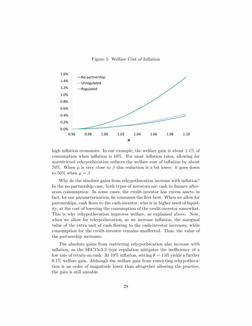
Figure 5: Welfare Cost of Inflation

0.0%

0.2%

0.4%

0.6%

0.8%

1.0%

1.2%

1.4%

1.6%

0.96 0.98 1.00 1.02 1.04 1.06 1.08 1.10

No partnershipUnregulatedRegulated

high inflation economies. In our example, the welfare gain is about 1.1% ofconsumption when inflation is 10%. For most inflation rates, allowing forunrestricted rehypothecation reduces the welfare cost of inflation by about70%. When µ is very close to β this reduction is a bit lower: it goes downto 50% when µ = β

Why do the absolute gains from rehypothecation increase with inflation?In the no partnership case, both types of investors use cash to finance after-noon consumption. In some cases, the credit-investor has excess assets–infact, for our parameterization, he consumes the first-best. When we allow forpartnerships, cash flows to the cash-investor, who is in higher need of liquid-ity, at the cost of lowering the consumption of the credit-investor somewhat.This is why rehypothecation improves welfare, as explained above. Now,when we allow for rehypothecation, as we increase inflation, the marginalvalue of the extra unit of cash flowing to the cash-investor increases, whileconsumption for the credit-investor remains unaffected. Thus, the value ofthe partnership increases.

The absolute gains from restricting rehypothecation also increase withinflation, as the SEC15c3-3 type regulation mitigates the inefficiency of alow rate of return on cash. At 10% inflation, setting θ = 1.05 yields a further0.1% welfare gain. Although the welfare gain from restricting rehypotheca-tion is an order of magnitude lower than altogether allowing the practice,the gain is still sizeable.

29

7 Discussion

Our paper is related to several other works studying the role of rehypotheca-tion on improving the allocation of liquidity, such as Kahn and Park (2015)and Maurin, Monnet and Gottardi (2015). These authors study rehypoth-ecation as an optimal contracting problem, stressing different frictions inthe economy. For example, in Kahn and Park (2015), collateral is neededto solve an agency problem, whereas it is needed in our model to solve acommitment problem.21 Kahn and Park (2015) emphasize the role of riskin collateral-return (repo fails). Maurin (2015) also demonstrates how rehy-pothecation risk can diminish the benefits of enhanced liquidity provision.Muley (2016) is the only other paper we are aware of that, like ours, tacklesthe question of how monetary policy interacts with the practice of rehypoth-ecation. Among other things, he finds that using interest on reserves maybe preferable to open market operations when collateral is scarce.22

Unlike the papers cited above, we study the role of rehypothecation onliquidity allocation in a dynamic monetary model. We think a monetarymodel is appropriate to study rehypothecation because the practice is fun-damentally related to liquidity creation. In particular, the rehypothecationof private assets must compete with liquidity substitutes, primarily in theform of government money and debt. Among other things, we are able touse our model to address the question of how monetary policy might affectthe practice and desirability of rehypothecation. Our theory predicts thatrehypothecation is less valuable in the low-inflation, low-interest rate envi-ronment prevailing since 2008. Perhaps this is one reason why the practicehas diminished in recent years, though obviously perceptions of risk andadded regulatory controls must also have played a significant role.

The model is also well-suited to exploring the economic impact andwelfare consequences of regulatory interventions designed to restrict rehy-pothecation. That regulatory restrictions on asset liquidity may in somecases improve overall liquidity is echoed in a related literature on assetliquidity in dynamic monetary models, such as Kocherlakota (2003), Shi(2008), Berentsen, Huber, Marchesiani (2014), Geromichalos and Herren-

21Although we do not model a lack of commitment within the risk-sharing arrangementhere, we have done so in an earlier version of our paper: Andolfatto, Martin and Zhang(2015, section 6).

22In some interesting related work that abstracts from liquidity issues, Eren (2014) andInfante (2015) study aspects of the counterparty risk that is commonly associated withthe practice of rehypothecation.

30

brueck (2016, 2017). None of these papers, however, specifically deal withthe issue of rehypothecation.

It would be of some interest to extend the model developed here to incor-porate aggregate uncertainty over returns on securities when commitmentbetween investors is limited. Consider a version of our model where the cash-investor wants a U.S. treasury (UST) bond and the credit-investor wants amortgage-backed-security (MBS). Imagine further that the conditional fore-cast over the future MBS dividend is subject to random “news shocks;” e.g.,see Andolfatto and Martin (2013). Then a “bad news” shock realized in theevening would unexpectedly lower the price of MBS and raise the price ofUSTs through a portfolio rebalance effect, e.g., see Andolfatto (2015). Thecash-investor is at this point is long MBS and short USTs, similar to theposition of Lehman Brothers in the fall of 2008 (Mackintosh, 2008). Themarket revaluation of his position makes it more costly for him to reacquirethe promised UST (or its value equivalent). If commitment is weak, thenthe UST borrower may strategically default. It would then be possible toinvestigate how monetary policy might be designed to accommodate spikesin “repo failures” in times of financial crisis (see Hordahl and King, 2008).

31

8 References

1. Andolfatto, David and Fernando Martin (2013). “Information Dis-closure and Exchange Media,” Review of Economic Dynamics, 16(3):527–539.

2. Andolfatto, David (2015). “A Model of U.S. Monetary Policy Beforeand After the Great Recession,” Federal Reserve Bank of St. LouisReview, 97(3): 233–256.

3. Andolfatto, David, Fernando Martin, Shengxing Zhang (2015). “Re-hypothecation and Liquidity,” Federal Reserve Bank of St. LouisWorking Paper Series, 2015-003B.

4. Aruoba, S. Boragan, Guillaume Rocheteau and Christopher Waller(2007). “Bargaining and the Value of Money”, Journal of MonetaryEconomics, 54: 2636–2655.

5. Berentsen, Aleksander, Samuel Huber, and Alessandro Marchesiani(2014). “Degreasing the Wheels of Finance.” International EconomicReview, 55 (3): 735–763.

6. Caballero, Ricardo (2006). “On the Macroeconomics of Asset Short-ages,” NBER working paper.

7. Duffie, Darrell, Nicolae Garleanu and Lasse Heje Pedersen (2005).“Over-The-Counter Markets,” Econometrica, 73(6): 1815–1847.

8. Eren, Egemen (2014). “Intermediary Funding Liquidity and Rehy-pothecation as Determinants of Repo Haircuts and Interest Rates,”manuscript.

9. Farhi, Emmanuel, Golosov, Mikhail and Aleh Tsyvinski (2009). “ATheory of Liquidity and Regulation of Financial Intermediation,” Re-view of Economic Studies, 76: 973-992.

10. Gale, Doug (1978). “The Core of a Monetary Economy without Trust,”Journal of Economic Theory, 19(2): 456–491.

11. Geromichalos, Athanasios, and Lucas Herrenbrueck (2016). ”Mone-tary Policy, Asset Prices, and Liquidity in Over-the-Counter Markets.”Journal of Money, Credit and Banking, 48(1), 35-79.

32

12. Geromichalos, Athanasios, and Lucas Herrenbrueck (2017), “A TractableModel of Indirect Asset Liquidity”, Journal of Economic Theory, Vol.168, March 2017, 252-260.

13. Geromichalos, Athanasios, Juan Licari and Jose Suarez-Lledo (2007).“Asset Prices and Monetary Policy,” Review of Economic Dynamics,Vol. 10, Issue 4, October 2007, 761–779.

14. Hordahl, Peter and Michael R. King (2008). “Developments in RepoMarkets During the Financial Crisis,” BIS Quarterly Review, 37–53.

15. International Capital Market Association. “Haircuts and initial mar-gins in the repo market,” European Repo Council (2012).

16. Infante, Sebastian (2015). “Liquidity Windfalls: The Consequencesof Repo Rehypothecation.” Finance and Economics Discussion Series2015-022. Washington: Board of Governors of the Federal ReserveSystem.

17. Kahn, Charles M., and Hye Jin Park (2015). “Collateral, rehypothe-cation, and efficiency.” UIUC, working paper.

18. Kocherlakota, Narayana (2003). “Societal benefits of illiquid bonds.”Journal of Economic Theory, 108(2), 179-193.

19. Lagos, Ricardo and Randall Wright (2005). “A Unified Framework forMonetary Theory and Policy Analysis,” Journal of Political Economy,113(3): 463–484.

20. Lester, Benjamin, Andrew Postlewaite, and Randall Wright. “Infor-mation, liquidity, asset prices, and monetary policy.” The Review ofEconomic Studies 79.3 (2012): 1209-1238.

21. Lucas, Robert E. (2000). “Inflation and Welfare,”Econometrica 68(2),247–274.

22. Macintosh, James (2008). “Lehman Collapse Puts Prime Broker Modelin Question,” Financial Times https://www.ft.com/content/442f0b24-8a71-11dd-a76a-0000779fd18c

23. Maurin, Vincent (2015). “Re-using Collateral of Others: A GeneralEquilibrium Model of Rehypothecation,” European University Institi-tute working paper.

33

24. Maurin, Vincent, Cyril Monnet, Piero Gottardi (2016), “A Theoryof Repurchase Agreements, Collateral Re-use and Intermediation,”Working paper.

25. Monnet, Cyril (2011). “Rehypothecation,” Federal Reserve Bank ofPhiladelphia Business Review, Q4, pp. 18–25.

26. Monnet, Cyril and Borghan Narajabad (2012). “Why Rent When YouCan Buy? A Theory of Repurchase Agreements,” manuscript.

27. Muley, Ameya (2016). “Rehypothecation and Monetary Policy,” Work-ing paper.

28. Rocheteau, Guillaume and Randall Wright (2004). “Inflation and Wel-fare in Models with Trading Frictions,” in Monetary Policy in LowInflation Economies, ed. by Dave Altig and Ed Nosal. Cambridge:Cambridge University Press.

29. Shi, Shouyong (2008). “Efficiency Improvement from Restricting theLiquidity of Nominal Bonds,” Journal of Monetary Economics 55,1025–37.

30. Shkolnik, Alexander (2015). “Systemic Risk in the Repo Market,”http://helper.ipam.ucla.edu/publications/fmws1/fmws1 12590.pdf

31. Singh, Manmohan, and James Aitken (2010). “The (Sizable) Roleof Rehypothecation in the Shadow Banking System,” IMF WorkingPaper 10/172.

34

Appendix

A Derivation of (EQM1)–(EQM8)

Here we derive the optimality conditions associated with the investor prob-lem (12) and (13). Lagrange multipliers are assigned as follows. Let ψ be themultiplier associated with the budget constraint, (6); λ with the liquidityconstraint, (7); χ1 and χ2 with the regulatory constraints, (R1) and (R2),respectively; ζ1 and ζ2 with the credit-investor’s non-negativity constraints,(9) and (10), respectively; and ζ3 with (4). Recall that (5) is implied by(R2).

The necessary first-order conditions for an optimum are:

u′(y1)− p [ψ + λ− ζ1] = 0 (19)

u′(y2)− pψ = 0 (20)

−λ+ ζ1 + ζ3 − θχ1 = 0 (21)

ζ2 − pφ2χ1 − χ2 = 0 (22)

Vm(m′, a′)− ψ + ζ1 = 0 (23)

Va(m′, a′)− pφ2ψ + ζ2 = 0 (24)

By the envelope theorem:

Bm(2m, 2a) = ψ + λ− ζ1 + θχ1/2 (25)

Ba(2m, 2a) = pφ2 [ψ + χ1/2]− ζ2 + (1 + ϑ)χ2/2 (26)

The demands for money and securities in the evening must satisfy:

1/p = βBm(2m+, 2a+) (27)

φ3 = βBa(2m+, 2a+) (28)

By the envelope theorem:

Vm(m′, a′) = 1/p (29)

Va(m′, a′) = φ3 + ω (30)

We restrict attention to stationary allocations where all real variablesare constant over time and nominal variables grow at rate µ. Combine (19),(25) and (27) to form,

35

µ = β[u′(y1) + θpχ1/2] (31)

When (R1) is slack (χ1 = 0), we get the standard result that µ > β impliesy1 < y∗.

Now combine (20), (22), (24), (26) and (28) to form:

φ3 = β(φ3 + ω)[(1 + ϑ)u′(y2) + (1− ϑ)− ϑpχ1]/2 (32)

From conditions (19), (23) and (29), we have

pλ = u′(y1)− 1 (33)

pψ = 1 + pζ1 (34)

which imply λ > 0 iff y1 < y∗ and ψ > 0 always.

Using (20), (23), (24), (29) and (30) we get

pζ1 = u′(y2)− 1 (35)

ζ2/φ2 = u′(y2)− 1 (36)

Note that if y2 = y∗, then u′(y2) = 1 and so (35)–(36) imply ζ1 = ζ2 = 0.

Finally, using (21), (22), (33)–(36) we get

pζ3 = u′(y1)− u′(y2) + θpχ1 (37)

pχ1 + χ2/φ2 = u′(y2)− 1 (38)

Clearly, if χ1 > 0 or χ2 > 0 then y2 < y∗.

We now invoke the market-clearing conditions m = M and a = 1. Cash-investors spend all of their cash (when µ = β, they weakly prefer to do so).Thus, (7) holds with equality. Together with the market-clearing condition,we have:

2M −m2 = py1 (39)

Finally, the regulatory constraints need to be satisfied in equilibrium. Usingthe market clearing conditions and (39) we obtain equilbrium expressionsfor the regulatory constraints (R1) and (R2):

a2 − 1 ≤ (θ/φ2)(y1 −M/p) (40)

a2 − 1 ≤ ϑ (41)

Clearly, both constraints cannot bind simultaneously, except in the non-generic case φ2ϑ = θ(y1 −M/p).

36

B Proofs

Proof of Lemma 1. Given that (10) implies a2 ≥ 2a − a′, the flowbudget constraint (6) implies 2m − m′ + pφ2a2 − py1 − py2 ≥ 2m − m′ +pφ2(2a − a′) − py1 − py2 ≥ 0. Note that (7) and (9) imply m′ ≥ 0. Thus,2m+ pφ2a2 − py1 − py2 ≥ 0. Given that(7) holds with equality (wlog whenµ = β), 2m− py1 = m2, which yields (8).

Proof of Proposition 1. Suppose µ = β. In an unregulated economy,χ1 = 0. From (31), we get y1 = y∗. Thus, (37) and (38) imply 1−u′(y2) ≥ 0and u′(y2) − 1 ≥ 0, respectively. It follows that u′(y2) = 1 and so y2 = y∗.

Proof of Proposition 2. Follows from (31) and χ1 = 0.

Proof of Proposition 3 and 4. See Section 5.

Proof of Proposition 5. From Proposition 1 we know that y1 = y2 = y∗

in an unregulated economy. Wlog, set m2 = M (which implies (M/p = y∗)and a2 = 1. Then, both (40) and (41) are trivially satisfied and so χ1 =χ2 = 0. The dividend threshold ω∗ was defined as one that implementsy2 = y∗ for ϑ = 0. Hence, wlog set a2 = 1 when ω ≥ ω∗ and so, both (40)and (41) are satisfied, which implies χ1 = χ2 = 0.

Proof of Lemma 2. Let θ ≥ 1 and assume χ1 > 0. Suppose ζ3 = 0. FromProposition 5 we know that µ = β implies χ1 = 0, so for this case to be anequilibrium it must be that µ > β. From (31) we have y1 < y∗ and from (38)we have y2 < y∗. Given y1 < y∗, (33) implies λ > 0 and thus, (7) holds withequality. Given y2 < y∗, (35) and (36) imply ζ1 > 0 and ζ2 > 0, respectively.Thus, m′ = 0 and a′ = a−a2. In addition, since ψ > 0 always, (6) holds withequality. These results imply that (8) holds with equality as well. Givenζ3 = 0 and χ1 > 0, (37) implies θpχ1 = u′(y2)− u′(y1) > 0. Thus, y1 > y2.Using (7) and (8), both holding with equality, implies 2m−m2 > m2+pφ2a2,which in equilibrium can be rearranged as 2(M−m2) > pφ2a2. Since χ1 > 0,the regulatory constraint (40) holds with equality, which using (40) can bewritten as: θ(M −m2) = pφ2(a2 − 1). These two expressions put togetherimply a2(1 − θ/2) > 1. Given a2 ∈ [0, 2], we need θ < 1 to satisfy thisinequality, a contradiction with θ ≥ 1.

Proof of Proposition 6. If ω ∈ [ω, ω∗) and ϑ < Γ(ω), or ω < ω for anyϑ ∈ [0, 1], then χ2 > 0 and (R2) is satisfied with equality: a2 = 1 + ϑ. By(38), y2 < y∗. Thus, (33), (35) and (36) imply λ > 0, ζ1 > 0 and ζ2 > 0,i.e., (7), (9) and (10) are all satisfied with equality. By Lemma 1, (8) holds

37

with equality as well. Given χ1 = 0, (31) implies u′(y1) = µ/β and thus,y1 < y∗ and independent of ϑ.

Suppose ζ3 = 0. Then, m2 ≥ 0 and by (35), y1 = y2. Thus, y2 is alsoindependent of ϑ. From Proposition 4, we know that ζ3 = 0 for ϑ = 1 onlyif ω < ω0(µ) and µ ∈ [β, 1). Thus, ζ3 = 0 for all ϑ ∈ [0, 1] only if ω < ω0(µ)and µ ∈ [β, 1).

Assume now ω ∈ [ω0(µ), ω∗) and ϑ such that (R2) binds. Then ζ3 > 0,i.e., m2 = 0 and by (35) y1 < y2. Since m2 = 0 and (8) holds with equality,y2 = φ2(1 +ϑ). Given that y2/(1 +ϑ) = φ2 = φ3 +ω, we can rewrite (32) as

y2 − (1 + ϑ)ω = (βy2/2)[(1 + ϑ)u′(y2) + (1− ϑ)]

Differentiate both sides by ϑ to obtain (after some rearrangement):

(1 + ϑ)(dy2/dϑ)[(2ω/y2)− βy2u′′(y2)

]= 2ω + βy2[u

′(y2)− 1]

Given u′(y2)− 1 > 0 and u′′(y2) < 0, we obtain dy2/dϑ > 0.

38