Rehashing Kernel Evaluation in High Dimensions11-14... · Intro Contribution Sketching Diagnostics...
80
Intro Contribution Sketching Diagnostics Evaluation Conclusion Rehashing Kernel Evaluation in High Dimensions Paris Siminelakis* Ph.D. Candidate Kexin Rong*, Peter Bailis, Moses Charikar, Phillip Levis (Stanford University) ICML @ Long Beach, California * equal contribution. June 11, 2019
Transcript of Rehashing Kernel Evaluation in High Dimensions11-14... · Intro Contribution Sketching Diagnostics...
Intro Contribution Sketching Diagnostics Evaluation Conclusion
Rehashing Kernel Evaluation in High Dimensions
Paris Siminelakis*Ph.D. Candidate
Kexin Rong*, Peter Bailis, Moses Charikar, Phillip Levis
(Stanford University)
ICML @ Long Beach, California
* equal contribution. June 11, 2019
Intro Contribution Sketching Diagnostics Evaluation Conclusion
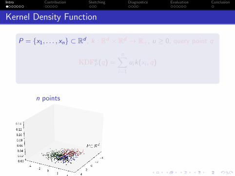
Kernel Density Function
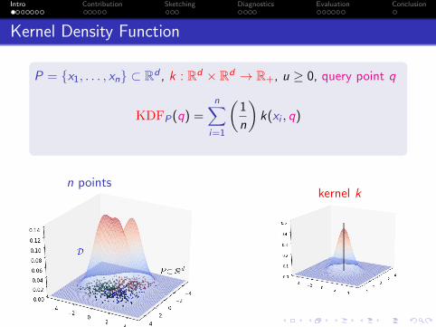
P = {x1, . . . , xn} ⊂ Rd , k : Rd × Rd → R+, u ≥ 0, query point q
KDFuP(q) =
n∑i=1
uik(xi , q)
n points
Intro Contribution Sketching Diagnostics Evaluation Conclusion
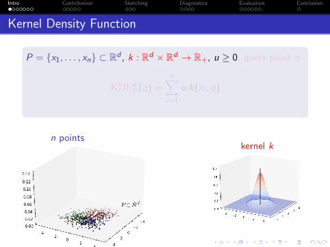
Kernel Density Function
P = {x1, . . . , xn} ⊂ Rd , k : Rd × Rd → R+, u ≥ 0, query point q
KDFuP(q) =
n∑i=1
uik(xi , q)
n pointskernel k
Intro Contribution Sketching Diagnostics Evaluation Conclusion
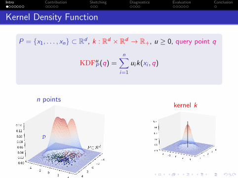
Kernel Density Function
P = {x1, . . . , xn} ⊂ Rd , k : Rd × Rd → R+, u ≥ 0, query point q
KDFuP(q) =
n∑i=1
uik(xi , q)
n pointskernel k
Intro Contribution Sketching Diagnostics Evaluation Conclusion
Kernel Density Function
P = {x1, . . . , xn} ⊂ Rd , k : Rd × Rd → R+, u ≥ 0, query point q
KDFP(q) =n∑
i=1
(1
n
)k(xi , q)
n pointskernel k
Intro Contribution Sketching Diagnostics Evaluation Conclusion
Kernel Density Evaluation
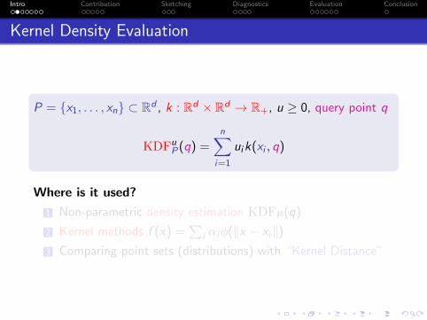
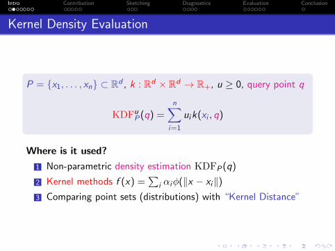
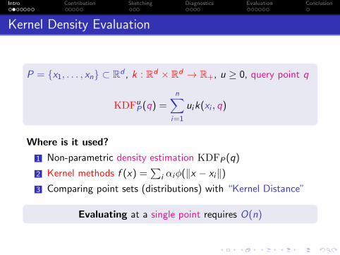
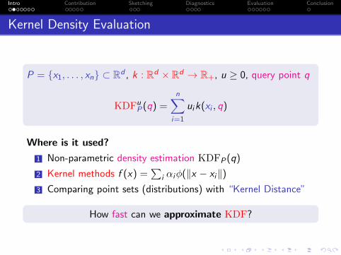
P = {x1, . . . , xn} ⊂ Rd , k : Rd × Rd → R+, u ≥ 0, query point q
KDFuP(q) =
n∑i=1
uik(xi , q)
Where is it used?
1 Non-parametric density estimation KDFP(q)
2 Kernel methods f (x) =∑
i αiφ(‖x − xi‖)3 Comparing point sets (distributions) with “Kernel Distance”
Intro Contribution Sketching Diagnostics Evaluation Conclusion
Kernel Density Evaluation
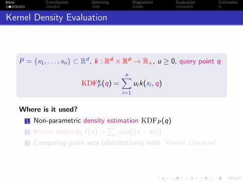
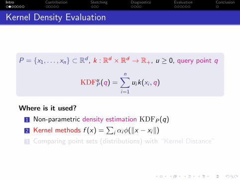
P = {x1, . . . , xn} ⊂ Rd , k : Rd × Rd → R+, u ≥ 0, query point q
KDFuP(q) =
n∑i=1
uik(xi , q)
Where is it used?
1 Non-parametric density estimation KDFP(q)
2 Kernel methods f (x) =∑
i αiφ(‖x − xi‖)3 Comparing point sets (distributions) with “Kernel Distance”
Evaluating at a single point requires O(n)
Intro Contribution Sketching Diagnostics Evaluation Conclusion
Kernel Density Evaluation
P = {x1, . . . , xn} ⊂ Rd , k : Rd × Rd → R+, u ≥ 0, query point q
KDFuP(q) =
n∑i=1
uik(xi , q)
Where is it used?
1 Non-parametric density estimation KDFP(q)
2 Kernel methods f (x) =∑
i αiφ(‖x − xi‖)3 Comparing point sets (distributions) with “Kernel Distance”
How fast can we approximate KDF?
Intro Contribution Sketching Diagnostics Evaluation Conclusion
Methods for Fast Kernel Evaluation
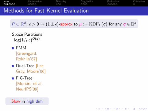
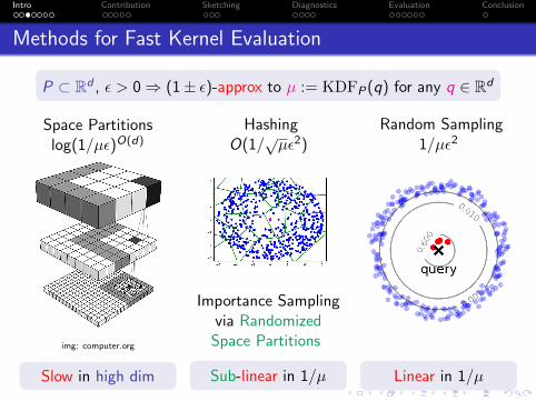
P ⊂ Rd , ε > 0⇒ (1± ε)-approx to µ := KDFP(q) for any q ∈ Rd
Intro Contribution Sketching Diagnostics Evaluation Conclusion
Methods for Fast Kernel Evaluation
P ⊂ Rd , ε > 0⇒ (1± ε)-approx to µ := KDFP(q) for any q ∈ Rd
Space Partitionslog(1/µε)O(d)
FMM[Greengard,Rokhlin’87]
Dual-Tree [Lee,Gray, Moore’06]
FIG-Tree[Moriaru et al.NeurIPS’09]
Slow in high dim
Intro Contribution Sketching Diagnostics Evaluation Conclusion
Methods for Fast Kernel Evaluation
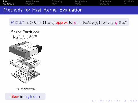
P ⊂ Rd , ε > 0⇒ (1± ε)-approx to µ := KDFP(q) for any q ∈ Rd
Space Partitionslog(1/µε)O(d)
img: computer.org
Slow in high dim
Intro Contribution Sketching Diagnostics Evaluation Conclusion
Methods for Fast Kernel Evaluation
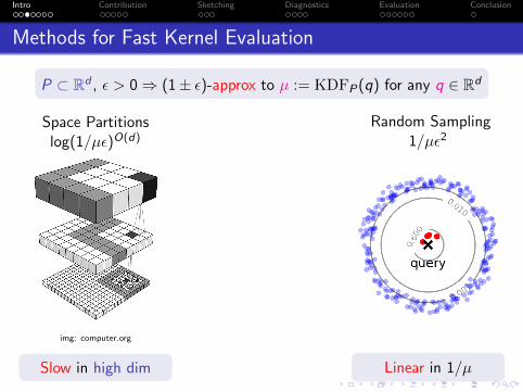
P ⊂ Rd , ε > 0⇒ (1± ε)-approx to µ := KDFP(q) for any q ∈ Rd
Space Partitionslog(1/µε)O(d)
img: computer.org
Slow in high dim
Random Sampling1/µε2
Linear in 1/µ
Intro Contribution Sketching Diagnostics Evaluation Conclusion
Methods for Fast Kernel Evaluation
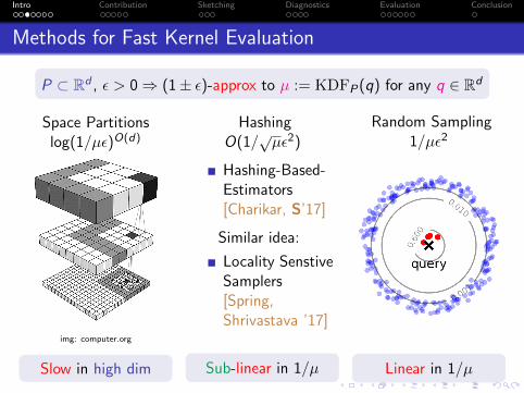
P ⊂ Rd , ε > 0⇒ (1± ε)-approx to µ := KDFP(q) for any q ∈ Rd
Space Partitionslog(1/µε)O(d)
img: computer.org
Slow in high dim
HashingO(1/
√µε2)
Hashing-Based-Estimators[Charikar, S’17]
Similar idea:
Locality SenstiveSamplers[Spring,Shrivastava ’17]
Sub-linear in 1/µ
Random Sampling1/µε2
Linear in 1/µ
Intro Contribution Sketching Diagnostics Evaluation Conclusion
Methods for Fast Kernel Evaluation
P ⊂ Rd , ε > 0⇒ (1± ε)-approx to µ := KDFP(q) for any q ∈ Rd
Space Partitionslog(1/µε)O(d)
img: computer.org
Slow in high dim
HashingO(1/
√µε2)
Importance Samplingvia Randomized
Space Partitions
Sub-linear in 1/µ
Random Sampling1/µε2
Linear in 1/µ
Intro Contribution Sketching Diagnostics Evaluation Conclusion
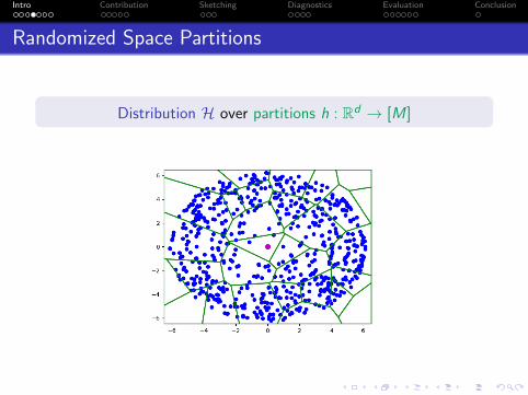
Randomized Space Partitions
Distribution H over partitions h : Rd → [M]
Intro Contribution Sketching Diagnostics Evaluation Conclusion
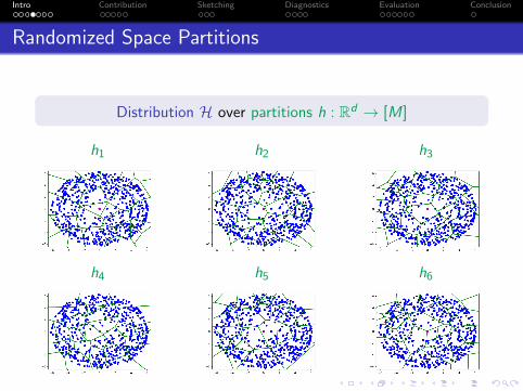
Randomized Space Partitions
Distribution H over partitions h : Rd → [M]
h1
h4
h2
h5
h3
h6
Intro Contribution Sketching Diagnostics Evaluation Conclusion
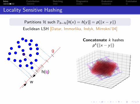
Locality Sensitive Hashing
Partitions H such Ph∼H[h(x) = h(y)] = p(‖x − y‖)Euclidean LSH [Datar, Immorlika, Indyk, Mirrokni’04]
Concatenate k hashespk(‖x − y‖)
Intro Contribution Sketching Diagnostics Evaluation Conclusion
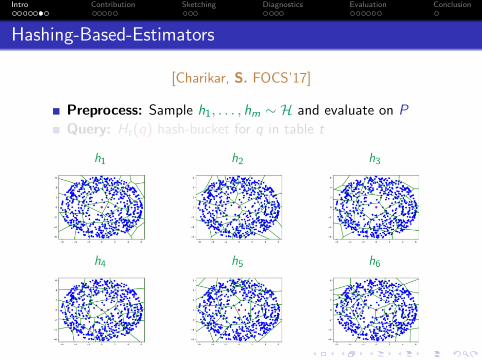
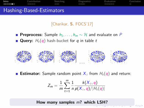
Hashing-Based-Estimators
[Charikar, S. FOCS’17]
Preprocess: Sample h1, . . . , hm ∼ H and evaluate on P
Query: Ht(q) hash-bucket for q in table t
Intro Contribution Sketching Diagnostics Evaluation Conclusion
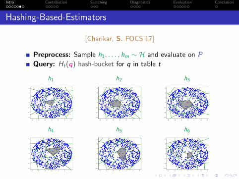
Hashing-Based-Estimators
[Charikar, S. FOCS’17]
Preprocess: Sample h1, . . . , hm ∼ H and evaluate on P
Query: Ht(q) hash-bucket for q in table t
Intro Contribution Sketching Diagnostics Evaluation Conclusion
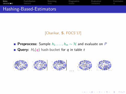
Hashing-Based-Estimators
[Charikar, S. FOCS’17]
Preprocess: Sample h1, . . . , hm ∼ H and evaluate on P
Query: Ht(q) hash-bucket for q in table t
· · ·
Intro Contribution Sketching Diagnostics Evaluation Conclusion
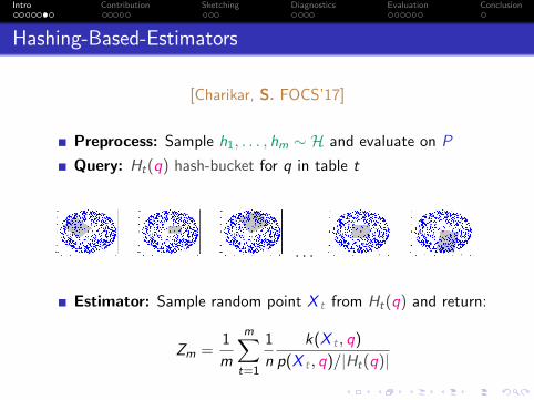
Hashing-Based-Estimators
[Charikar, S. FOCS’17]
Preprocess: Sample h1, . . . , hm ∼ H and evaluate on P
Query: Ht(q) hash-bucket for q in table t
· · ·
Estimator: Sample random point X t from Ht(q) and return:
Zm =1
m
m∑t=1
1
n
k(X t , q)
p(X t , q)/|Ht(q)|
Intro Contribution Sketching Diagnostics Evaluation Conclusion
Hashing-Based-Estimators
[Charikar, S. FOCS’17]
Preprocess: Sample h1, . . . , hm ∼ H and evaluate on P
Query: Ht(q) hash-bucket for q in table t
· · ·
Estimator: Sample random point X t from Ht(q) and return:
Zm =1
m
m∑t=1
1
n
k(X t , q)
p(X t , q)/|Ht(q)|
How many samples m? which LSH?
Intro Contribution Sketching Diagnostics Evaluation Conclusion
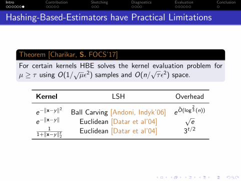
Hashing-Based-Estimators have Practical Limitations
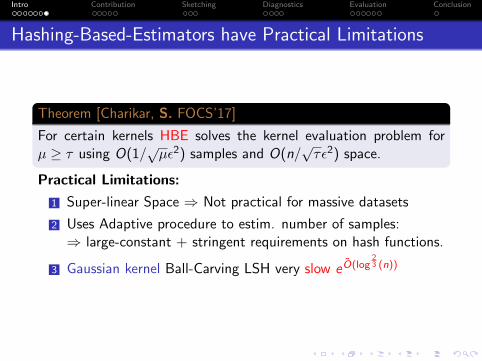
Theorem [Charikar, S. FOCS’17]
For certain kernels HBE solves the kernel evaluation problem forµ ≥ τ using O(1/
√µε2) samples and O(n/
√τε2) space.
Kernel LSH Overhead
e−‖x−y‖2
Ball Carving [Andoni, Indyk’06] eO(log23 (n))
e−‖x−y‖ Euclidean [Datar et al’04]√e
11+‖x−y‖t2
Euclidean [Datar et al’04] 3t/2
Intro Contribution Sketching Diagnostics Evaluation Conclusion
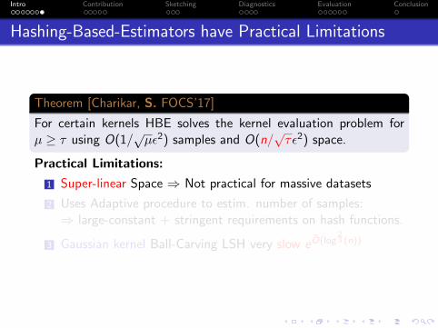
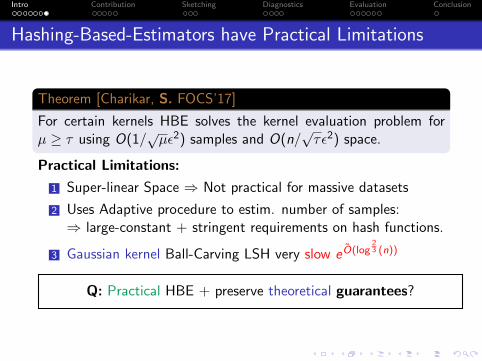
Hashing-Based-Estimators have Practical Limitations
Theorem [Charikar, S. FOCS’17]
For certain kernels HBE solves the kernel evaluation problem forµ ≥ τ using O(1/
√µε2) samples and O(n/
√τε2) space.
Practical Limitations:
1 Super-linear Space ⇒ Not practical for massive datasets
2 Uses Adaptive procedure to estim. number of samples:⇒ large-constant + stringent requirements on hash functions.
3 Gaussian kernel Ball-Carving LSH very slow eO(log23 (n))
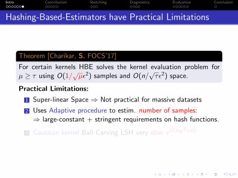
Intro Contribution Sketching Diagnostics Evaluation Conclusion
Hashing-Based-Estimators have Practical Limitations
Theorem [Charikar, S. FOCS’17]
For certain kernels HBE solves the kernel evaluation problem forµ ≥ τ using O(1/
√µε2) samples and O(n/
√τε2) space.
Practical Limitations:
1 Super-linear Space ⇒ Not practical for massive datasets
2 Uses Adaptive procedure to estim. number of samples:⇒ large-constant + stringent requirements on hash functions.
3 Gaussian kernel Ball-Carving LSH very slow eO(log23 (n))
Q: Practical HBE + preserve theoretical guarantees?
Intro Contribution Sketching Diagnostics Evaluation Conclusion
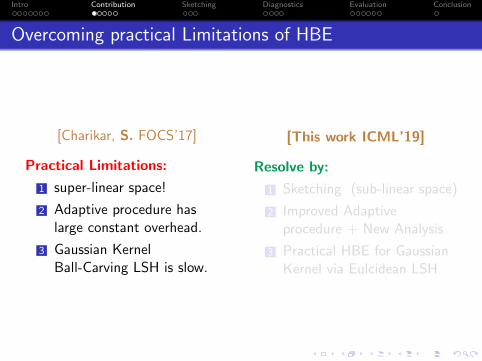
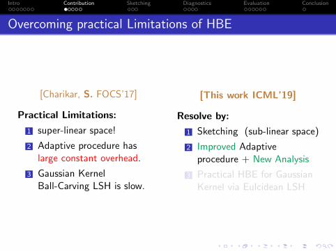
Overcoming practical Limitations of HBE
[Charikar, S. FOCS’17]
Practical Limitations:
1 super-linear space!
2 Adaptive procedure haslarge constant overhead.
3 Gaussian KernelBall-Carving LSH is slow.
[This work ICML’19]
Resolve by:
1 Sketching (sub-linear space)
2 Improved Adaptiveprocedure + New Analysis
3 Practical HBE for GaussianKernel via Eulcidean LSH
Intro Contribution Sketching Diagnostics Evaluation Conclusion
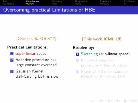
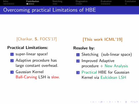
Overcoming practical Limitations of HBE
[Charikar, S. FOCS’17]
Practical Limitations:
1 super-linear space!
2 Adaptive procedure haslarge constant overhead.
3 Gaussian KernelBall-Carving LSH is slow.
[This work ICML’19]
Resolve by:
1 Sketching (sub-linear space)
2 Improved Adaptiveprocedure + New Analysis
3 Practical HBE for GaussianKernel via Eulcidean LSH
Intro Contribution Sketching Diagnostics Evaluation Conclusion
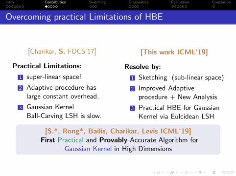
Overcoming practical Limitations of HBE
[Charikar, S. FOCS’17]
Practical Limitations:
1 super-linear space!
2 Adaptive procedure haslarge constant overhead.
3 Gaussian KernelBall-Carving LSH is slow.
[This work ICML’19]
Resolve by:
1 Sketching (sub-linear space)
2 Improved Adaptiveprocedure + New Analysis
3 Practical HBE for GaussianKernel via Eulcidean LSH
[S.*, Rong*, Bailis, Charikar, Levis ICML’19]First Practical and Provably Accurate Algorithm for
Gaussian Kernel in High Dimensions
Intro Contribution Sketching Diagnostics Evaluation Conclusion
Going back a step
Q1: Practical HBE + preserve theoretical guarantees?
Intro Contribution Sketching Diagnostics Evaluation Conclusion
Going back a step
Q1: Practical HBE + preserve theoretical guarantees?
Yes: Sketching, Adaptive procedure, Euclidean LSH
Intro Contribution Sketching Diagnostics Evaluation Conclusion
Going back a step
Q1: Practical HBE + preserve theoretical guarantees?
Yes: Sketching, Adaptive procedure, Euclidean LSH
Q2: Is it always better to use?
Intro Contribution Sketching Diagnostics Evaluation Conclusion
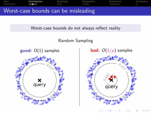
Worst-case bounds can be misleading
Worst-case bounds do not always reflect reality
Random Sampling
good: O(1) samples bad: O(1/µ) samples
Intro Contribution Sketching Diagnostics Evaluation Conclusion
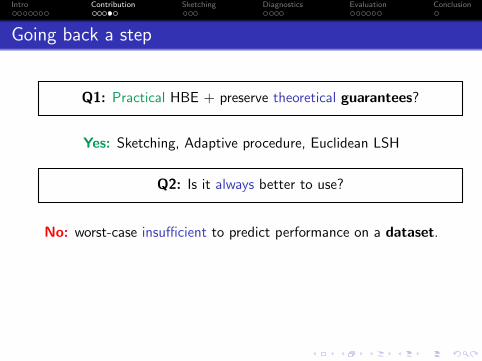
Going back a step
Q1: Practical HBE + preserve theoretical guarantees?
Yes: Sketching, Adaptive procedure, Euclidean LSH
Q2: Is it always better to use?
Intro Contribution Sketching Diagnostics Evaluation Conclusion
Going back a step
Q1: Practical HBE + preserve theoretical guarantees?
Yes: Sketching, Adaptive procedure, Euclidean LSH
Q2: Is it always better to use?
No: worst-case insufficient to predict performance on a dataset.
Intro Contribution Sketching Diagnostics Evaluation Conclusion
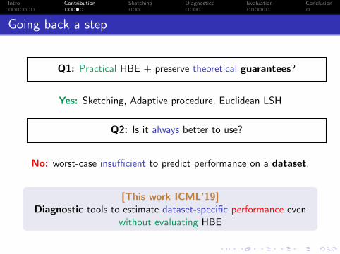
Going back a step
Q1: Practical HBE + preserve theoretical guarantees?
Yes: Sketching, Adaptive procedure, Euclidean LSH
Q2: Is it always better to use?
No: worst-case insufficient to predict performance on a dataset.
[This work ICML’19]Diagnostic tools to estimate dataset-specific performance even
without evaluating HBE
Intro Contribution Sketching Diagnostics Evaluation Conclusion
Outline of the rest of the talk
1 Sketching
2 Diagnostic tools
3 Experimental evaluation
Intro Contribution Sketching Diagnostics Evaluation Conclusion
Sketching
Intro Contribution Sketching Diagnostics Evaluation Conclusion
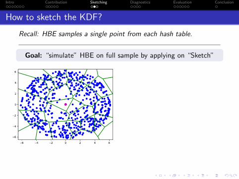
How to sketch the KDF?
Recall: HBE samples a single point from each hash table.
Goal: “simulate” HBE on full sample by applying on “Sketch”
Intro Contribution Sketching Diagnostics Evaluation Conclusion
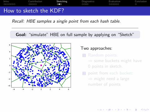
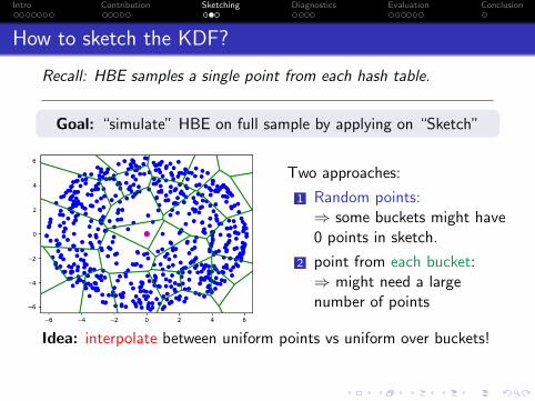
How to sketch the KDF?
Recall: HBE samples a single point from each hash table.
Goal: “simulate” HBE on full sample by applying on “Sketch”
Two approaches:
1 Random points:⇒ some buckets might have0 points in sketch.
2 point from each bucket:⇒ might need a largenumber of points
Intro Contribution Sketching Diagnostics Evaluation Conclusion
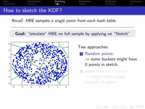
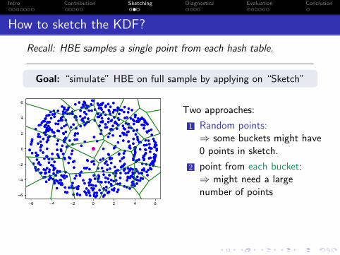
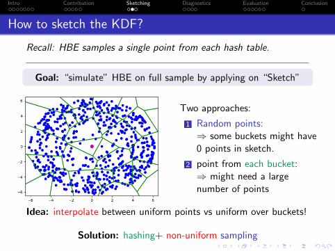
How to sketch the KDF?
Recall: HBE samples a single point from each hash table.
Goal: “simulate” HBE on full sample by applying on “Sketch”
Two approaches:
1 Random points:⇒ some buckets might have0 points in sketch.
2 point from each bucket:⇒ might need a largenumber of points
Idea: interpolate between uniform points vs uniform over buckets!
Intro Contribution Sketching Diagnostics Evaluation Conclusion
How to sketch the KDF?
Recall: HBE samples a single point from each hash table.
Goal: “simulate” HBE on full sample by applying on “Sketch”
Two approaches:
1 Random points:⇒ some buckets might have0 points in sketch.
2 point from each bucket:⇒ might need a largenumber of points
Idea: interpolate between uniform points vs uniform over buckets!
Solution: hashing+ non-uniform sampling
Intro Contribution Sketching Diagnostics Evaluation Conclusion
Sketching Kernel Density Function
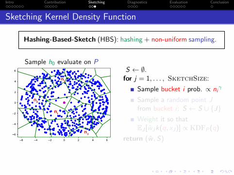
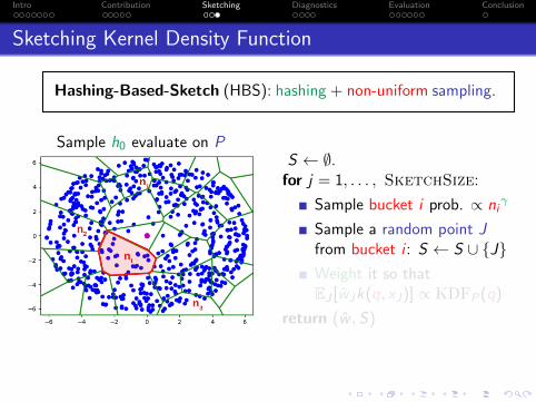
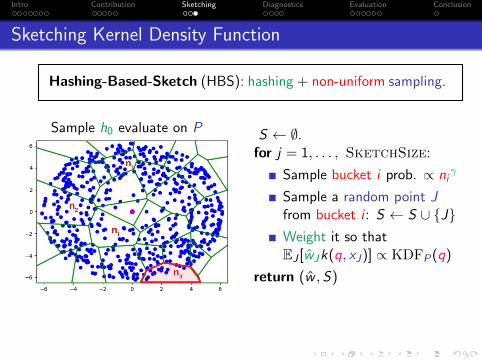
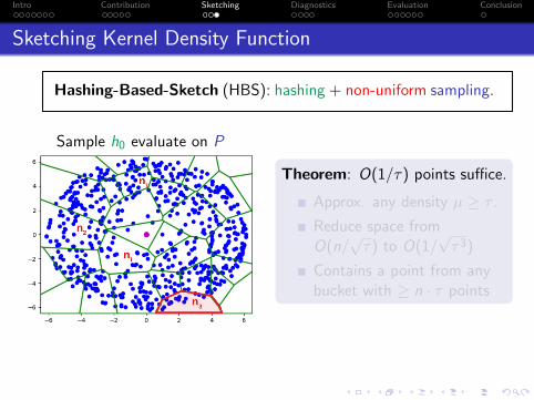
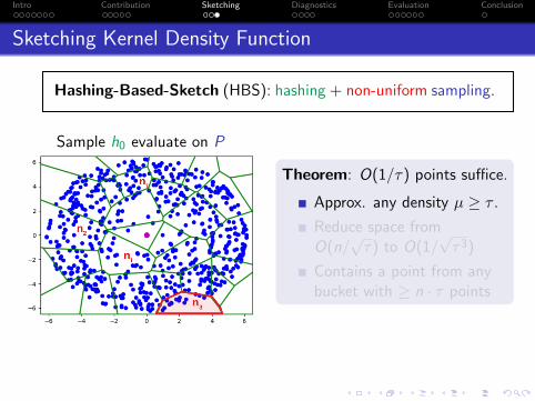
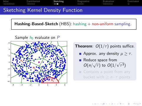
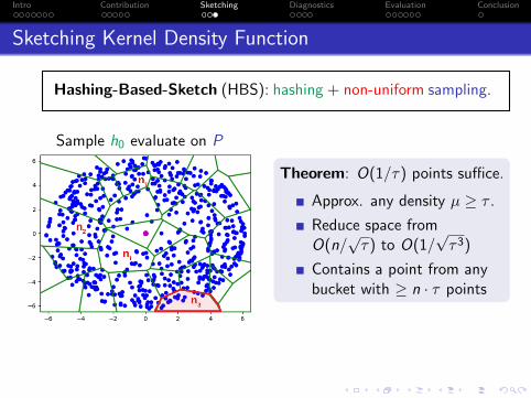
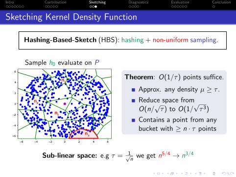
Hashing-Based-Sketch (HBS): hashing + non-uniform sampling.
Intro Contribution Sketching Diagnostics Evaluation Conclusion
Sketching Kernel Density Function
Hashing-Based-Sketch (HBS): hashing + non-uniform sampling.
Sample h0 evaluate on P
Intro Contribution Sketching Diagnostics Evaluation Conclusion
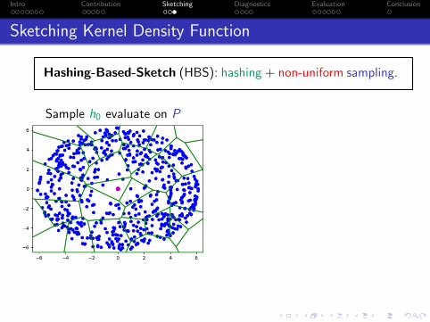
Sketching Kernel Density Function
Hashing-Based-Sketch (HBS): hashing + non-uniform sampling.
Sample h0 evaluate on PS ← ∅.for j = 1, . . . , SketchSize:
Sample bucket i prob. ∝ niγ
Sample a random point Jfrom bucket i : S ← S ∪ {J}Weight it so thatEJ [wJk(q, xJ)] ∝ KDFP(q)
return (w , S)
Intro Contribution Sketching Diagnostics Evaluation Conclusion
Sketching Kernel Density Function
Hashing-Based-Sketch (HBS): hashing + non-uniform sampling.
Sample h0 evaluate on P S ← ∅.for j = 1, . . . , SketchSize:
Sample bucket i prob. ∝ niγ
Sample a random point Jfrom bucket i : S ← S ∪ {J}Weight it so thatEJ [wJk(q, xJ)] ∝ KDFP(q)
return (w , S)
Intro Contribution Sketching Diagnostics Evaluation Conclusion
Sketching Kernel Density Function
Hashing-Based-Sketch (HBS): hashing + non-uniform sampling.
Sample h0 evaluate on P
Theorem: O(1/τ) points suffice.
Approx. any density µ ≥ τ .
Reduce space fromO(n/
√τ) to O(1/
√τ3)
Contains a point from anybucket with ≥ n · τ points
Sub-linear space: e.g τ = 1√n
we get n5/4 → n3/4
Intro Contribution Sketching Diagnostics Evaluation Conclusion
Diagnostic tools
Intro Contribution Sketching Diagnostics Evaluation Conclusion
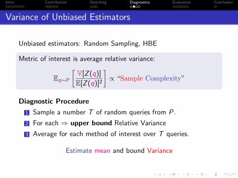
Variance of Unbiased Estimators
Unbiased estimators: Random Sampling, HBE
Metric of interest is average relative variance:
Eq∼P
[V[Z (q)]
E[Z (q)]2
]∝ “Sample Complexity”
Diagnostic Procedure
1 Sample a number T of random queries from P.
2 For each ⇒ upper bound Relative Variance
3 Average for each method of interest over T queries.
Estimate mean and bound Variance
Intro Contribution Sketching Diagnostics Evaluation Conclusion
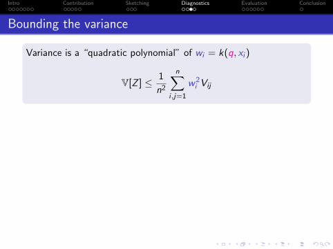
Bounding the variance
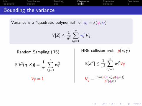
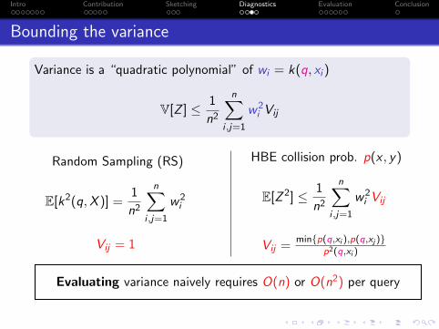
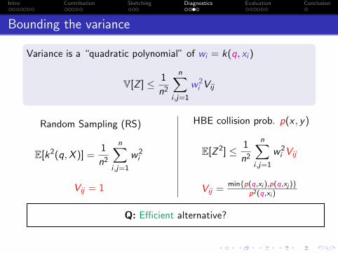
Variance is a “quadratic polynomial” of wi = k(q, xi )
V[Z ] ≤ 1
n2
n∑i ,j=1
w2i Vij
Intro Contribution Sketching Diagnostics Evaluation Conclusion
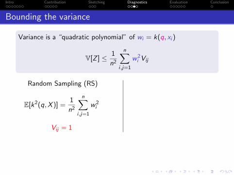
Bounding the variance
Variance is a “quadratic polynomial” of wi = k(q, xi )
V[Z ] ≤ 1
n2
n∑i ,j=1
w2i Vij
Random Sampling (RS)
E[k2(q,X )] =1
n2
n∑i ,j=1
w2i
Vij = 1
Intro Contribution Sketching Diagnostics Evaluation Conclusion
Bounding the variance
Variance is a “quadratic polynomial” of wi = k(q, xi )
V[Z ] ≤ 1
n2
n∑i ,j=1
w2i Vij
Random Sampling (RS)
E[k2(q,X )] =1
n2
n∑i ,j=1
w2i
Vij = 1
HBE collision prob. p(x , y)
E[Z 2] ≤ 1
n2
n∑i ,j=1
w2i Vij
Vij =min{p(q,xi ),p(q,xj )}
p2(q,xi )
Evaluating variance naively requires O(n) or O(n2) per query
Intro Contribution Sketching Diagnostics Evaluation Conclusion
Bounding the variance
Variance is a “quadratic polynomial” of wi = k(q, xi )
V[Z ] ≤ 1
n2
n∑i ,j=1
w2i Vij
Random Sampling (RS)
E[k2(q,X )] =1
n2
n∑i ,j=1
w2i
Vij = 1
HBE collision prob. p(x , y)
E[Z 2] ≤ 1
n2
n∑i ,j=1
w2i Vij
Vij =min{p(q,xi ),p(q,xj )}
p2(q,xi )
Q: Efficient alternative?
Intro Contribution Sketching Diagnostics Evaluation Conclusion
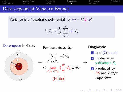
Data-dependent Variance Bounds
Variance is a “quadratic polynomial” of wi = k(q, xi )
V[Z ] ≤ 1
n2
n∑i ,j=1
w2i Vij
Decompose in 4 sets
→
For two sets S`,S`′ :∑i∈S`,j∈S`′
w2i Vij
≤ supi∈S`,j∈S`′
{wi
wjVij}µ`µ`′
(Holder)
→
Diagnostic
1 bnd(42
)terms
2 Evaluate onsubsample S0
3 Produced byRS and Adapt.Algorithm
Intro Contribution Sketching Diagnostics Evaluation Conclusion
Evaluation
Intro Contribution Sketching Diagnostics Evaluation Conclusion
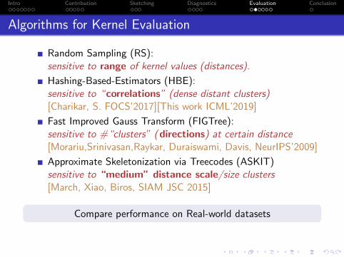
Algorithms for Kernel Evaluation
Random Sampling (RS):sensitive to range of kernel values (distances).
Hashing-Based-Estimators (HBE):sensitive to “correlations” (dense distant clusters)[Charikar, S. FOCS’2017][This work ICML’2019]
Fast Improved Gauss Transform (FIGTree):sensitive to #“clusters” (directions) at certain distance[Morariu,Srinivasan,Raykar, Duraiswami, Davis, NeurIPS’2009]
Approximate Skeletonization via Treecodes (ASKIT)sensitive to “medium” distance scale/size clusters[March, Xiao, Biros, SIAM JSC 2015]
Compare performance on Real-world datasets
Intro Contribution Sketching Diagnostics Evaluation Conclusion
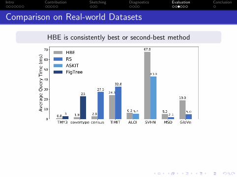
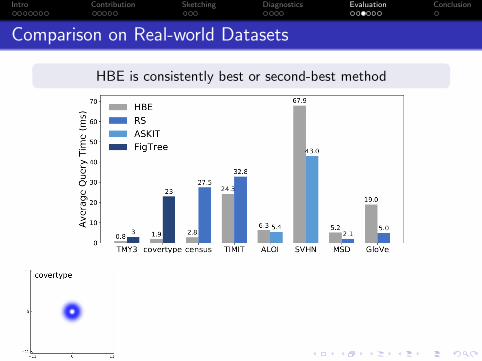
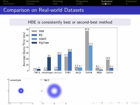
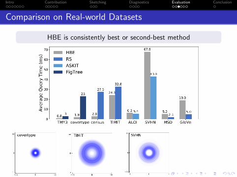
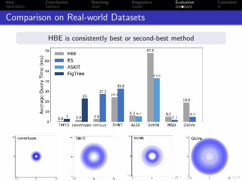
Comparison on Real-world Datasets
HBE is consistently best or second-best method
Intro Contribution Sketching Diagnostics Evaluation Conclusion
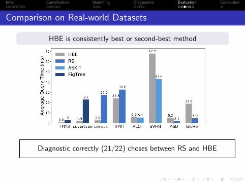
Comparison on Real-world Datasets
HBE is consistently best or second-best method
Diagnostic correctly (21/22) choses between RS and HBE
Intro Contribution Sketching Diagnostics Evaluation Conclusion
Comparison on Real-world Datasets
HBE is consistently best or second-best method
Intro Contribution Sketching Diagnostics Evaluation Conclusion
Comparison on Real-world Datasets
HBE is consistently best or second-best method
Intro Contribution Sketching Diagnostics Evaluation Conclusion
Comparison on Real-world Datasets
HBE is consistently best or second-best method
Intro Contribution Sketching Diagnostics Evaluation Conclusion
Comparison on Real-world Datasets
HBE is consistently best or second-best method
Intro Contribution Sketching Diagnostics Evaluation Conclusion
Benchmark Instances
Synthetic Benchmarks:
1 Worst-case: no single geometric aspect can be exploited!
2 D-clusters: gauge impact of different geometric aspects.
Intro Contribution Sketching Diagnostics Evaluation Conclusion
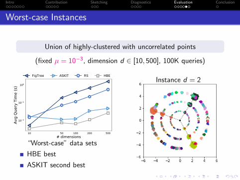
Worst-case Instances
Union of highly-clustered with uncorrelated points
(fixed µ = 10−3, dimension d ∈ [10, 500], 100K queries)
10 50 100 200 500# dimensions
10−2
10−1
100
Avg
Quer
y Ti
me
(s)
FigTree ASKIT RS HBE
“Worst-case” data sets
HBE best
ASKIT second best
Instance d = 2
Intro Contribution Sketching Diagnostics Evaluation Conclusion
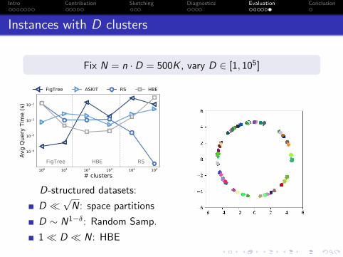
Instances with D clusters
Fix N = n · D = 500K , vary D ∈ [1, 105]
100 101 102 103 104 105
# clusters
10−4
10−3
10−2
10−1
Avg
Quer
y Ti
me
(s)
FigTree HBE RS
FigTree ASKIT RS HBE
D-structured datasets:
D �√N: space partitions
D ∼ N1−δ: Random Samp.
1� D � N: HBE
Intro Contribution Sketching Diagnostics Evaluation Conclusion
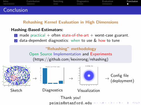
Conclusion
Rehashing Kernel Evaluation in High Dimensions
Hashing-Based-Estimators:
1 made practical + often state-of-the-art + worst-case guarant.2 data-dependent diagnostics: when to use & how to tune
“Rehashing” methodologyOpen Source Implementation and Experiments
(https://github.com/kexinrong/rehashing)
Sketch
→
Diagnostics
→
Visualization
→ Config file(deployment)
Thank [email protected]