Regulatory Impact Analysis (RIA) for Residential Wood ... · Regulatory Impact Analysis (RIA) for...
203
Regulatory Impact Analysis (RIA) for Residential Wood Heaters NSPS Revision Final Report
Transcript of Regulatory Impact Analysis (RIA) for Residential Wood ... · Regulatory Impact Analysis (RIA) for...
Regulatory Impact Analysis (RIA) for
Residential Wood Heaters NSPS Revision
Final Report

.
February 2015 EPA-452/R-15-001
U.S. Environmental Protection Agency
Office of Air and Regulation
Office of Air Quality Planning and Standards
Health and Environmental Impacts Division
The EPA wishes to acknowledge the contributions of the Research Triangle Institute (RTI)
International in the preparation of the industry profile and economic impact analysis, and EC/R,
Inc. in the preparation of the emissions and cost estimates included in this report.

iii
CONTENTS
Section Page
Section 1 Executive Summary ............................................................................................... 1-1
1.1 Analysis Summary ............................................................................................... 1-3
1.2 Organization of this Report .................................................................................. 1-5
Section 2 Introduction ............................................................................................................ 2-1
2.1 Background for Rule ............................................................................................ 2-1
2.2 Room Heaters....................................................................................................... 2-2
2.3 Central Heaters: Hydronic Heaters and Forced-Air Furnaces ............................. 2-8
Section 3 Industry Profile ...................................................................................................... 3-1
3.1 Supply Side .......................................................................................................... 3-1
3.1.1 Production Process ................................................................................... 3-2
3.1.2 Product Types .......................................................................................... 3-2
3.1.3 Costs of Production .................................................................................. 3-5
3.2 Demand Side ........................................................................................................ 3-8
3.2.1 End-Use Consumer Segments................................................................ 3-10
3.2.2 Regional Variation in Residential Demand ........................................... 3-10
3.2.3 National Home Heating Trends ............................................................. 3-13
3.2.4 Substitution Possibilities ........................................................................ 3-15
3.2.5 Price Elasticity of Demand .................................................................... 3-16
3.3 Industry Organization ........................................................................................ 3-17
3.3.1 Market Structure .................................................................................... 3-17
3.3.2 Manufacturing Plants ............................................................................. 3-19
3.3.3 Location ................................................................................................. 3-20
3.3.4 Company Sales and Employment .......................................................... 3-21
3.4 Residential Wood Heater Market....................................................................... 3-23
3.4.1 Market Prices ......................................................................................... 3-24

iv
3.4.2 International Competition ...................................................................... 3-25
3.4.3 Future Market Trends ............................................................................ 3-26
Section 4 Baseline Emissions and Emission Reductions ....................................................... 4-1
4.1 Introduction .......................................................................................................... 4-1
4.2 Background to Emissions Estimates .................................................................... 4-1
4.2.1 Emissions Factors .................................................................................... 4-4
4.2.2 Voluntary Programs ............................................................................... 4-11
4.2.3 Shipment Data Used to Estimate Baseline Emissions ........................... 4-12
4.3 Estimated PM2.5 Emissions from Shipments of New Appliances ..................... 4-14
4.4 Methodology for Estimating VOC Emissions from New Units ........................ 4-20
4.5 Methodology for Estimating CO Emissions from New Units ........................... 4-26
Section 5 Cost Analysis, Energy Impacts, and Executive Order Analyses ........................... 5-1
5.1 Background for Compliance Costs ...................................................................... 5-1
5.1.1 Estimated Research and Development (R&D) Costs .............................. 5-1
5.1.3 General Approach and Assumptions for Costs to Manufacturers .......... 5-10
5.1.4. Estimated Manufacturer Costs – Specific Assumptions &
Resulting Costs ...................................................................................... 5-13
5.2 Compliance Costs of the Rule as Presented in the RIA ..................................... 5-18
5.3 How Might People and Firms Respond? A Qualitative Partial Equilibrium
Analysis.............................................................................................................. 5-20
5.3.1 Changes in Market Prices and Quantities .............................................. 5-21
5.3.2 Partial Equilibrium Measures of Social Cost: Changes in
Consumer and Producer Surplus ............................................................ 5-25
5.4 Social Cost Estimate .......................................................................................... 5-26
5.5 Energy Impacts .................................................................................................. 5-26
5.6 Unfunded Mandates Reform Act (UMRA) ....................................................... 5-27
5.6.1 Future and Disproportionate Costs ........................................................ 5-27
5.6.3 Executive Order 13045: Protection of Children from
Environmental Health Risks and Safety Risks ...................................... 5-28

v
5.6.4 Executive Order 12898: Federal Actions to Address Environmental
Justice in Minority Populations and Low-Income Populations ............. 5-29
5.7 Employment Impacts ......................................................................................... 5-30
Section 6 Small Entity Screening Analysis ........................................................................... 6-1
6.1 Small Entity Data Set ........................................................................................... 6-1
6.2 Small Entity Economic Impact Measures ............................................................ 6-2
6.2.1 Establishment Employment and Receipts ................................................ 6-2
6.2.2 Establishment Compliance Cost .............................................................. 6-3
6.4 Final Regulatory Flexibility Analysis (FRFA) .................................................. 6-12
6.4.1 Reasons Why Action Is Being Considered ............................................ 6-12
6.4.2 Statement of Objectives and Legal Basis of Proposed Rule .................. 6-13
6.4.4 Description and Estimate of the Number of Small Entities ................... 6-13
6.4.5 Description of Impact Methodology and Compliance Costs ................. 6-13
6.4.5 Panel Recommendations for Small Business Flexibilities..................... 6-13
Section 7 Human Health Benefits of Emissions Reductions ................................................. 7-1
7.1 Synopsis ............................................................................................................... 7-1
7.2 PM2.5-Related Human Health Benefits ................................................................ 7-1
7.2.1 Health Impact Assessment ....................................................................... 7-2
7.2.2 Economic Valuation................................................................................. 7-6
7.2.3 Benefit-per-ton Estimates ........................................................................ 7-7
7.2.4 PM2.5 Benefits Results .............................................................................. 7-9
7.2.5 Characterization of Uncertainty in the Monetized PM2.5 Benefits ......... 7-11
7.3 Unquantified Benefits ........................................................................................ 7-17
7.3.1 HAP Benefits ......................................................................................... 7-19
7.3.2 Carbon Monoxide Co-Benefits .............................................................. 7-30
7.3.3 Black Carbon (BC) Benefits .................................................................. 7-31
7.3.4 VOCs as a PM2.5 Precursor .................................................................... 7-33
7.3.5 VOCs as an Ozone Precursor ................................................................. 7-34
7.3.6 Visibility Impairment Co-Benefits ........................................................ 7-34
7.4 References .......................................................................................................... 7-35

vi
Section 8 Comparison of Monetized Benefits and Costs ....................................................... 8-1
8.1 Summary .............................................................................................................. 8-1
Section 9 References And Cost APPENDIX ......................................................................... 9-1
vii
LIST OF FIGURES
Number Page
3-1. Census Regions and Divisions of the United States ................................................... 3-13
3-2. Declining Trend in U.S. Housing Units Using Wood Fuel: 1989–2005 .................... 3-14
3-3. Annual Plant Capacity Utilization for Heating Equipment Manufacturers
(NAICS 333414): 2002–2006 ..................................................................................... 3-19
5-1. Market Demand and Supply Model: With and Without Regulation .......................... 5-22
7-1. Total Monetized PM2.5 Benefits of the Residential Wood Heaters NSPS in the
2015–2020 Time Frame .............................................................................................. 7-12
7-2. Breakdown of Total Monetized PM2.5 Benefits of Residential Wood Heaters
NSPS by Category ...................................................................................................... 7-13
7-3. Percentage of Adult Population by Annual Mean PM2.5 Exposure in the
Baseline ....................................................................................................................... 7-18
7-4. Cumulative Distribution of Adult Population by Annual Mean PM2.5 Exposure
in the Baseline ............................................................................................................. 7-20
7-5. 2005 NATA Model Estimated Census Tract Carcinogenic Risk from HAP
Exposure from Emissions of all Outdoor Sources (inclusive of Residential
Wood Heaters) based on the 2005 National Toxic Inventory) ................................... 7-22
7-6. 2005 NATA Model Estimated Census Tract Noncancer Risk from HAP
Exposure from Emissions of all Outdoor Sources (inclusive of Residential
Wood Heaters) based on the 2005 National Toxic Inventory..................................... 7-24
8-1. Net Annual Benefits Range in 2015–2020 Time Frame for PM2.5 Reductions for
the NSPS With Benefits Discounted at 3% ................................................................. 8-3
8-2. Net Annual Benefits Range in 2015-2020 Time Frame for PM2.5 Reductions for the
NSPS With Benefits Discounted at 7%.........................................................................8-4
viii
LIST OF TABLES
Number Page
1-1. Summary of the Monetized Benefits, Social Costs, and Net Benefits for the
Residential Wood Heaters NSPS in the 2015–2020 Time Frame ($2013
millions) ........................................................................................................................ 1-7
2-1. Subpart AAA Compliance Deadlines and PM Emissions Limits ................................ 2-4
2-2. Subpart QQQQ Compliance Dates and PM Emissions Standards ............................. 2-10
3-1. Costs for Labor and Materials for U.S. Heating Equipment and Hardware
Manufacturing: 2011 ..................................................................................................... 3-7
3-2. Costs for Single-Family Home Contractors: 2007........................................................ 3-9
3-3. Costs for U.S. Plumbing and Heating Equipment Supplies Wholesalers: 2007 ........... 3-9
3-4. Costs for U.S. Specialized Home Furnishing Stores: 2007 .......................................... 3-9
3-5. Wood as Primary Fuel Source for Home Heating in the United States: 2006–
2008............................................................................................................................. 3-11
3-6. Wood as Secondary Heat Source by Census Division, 2009 (millions of
households) ................................................................................................................. 3-12
3-7. Number of U.S. Companies by Business Type........................................................... 3-20
3-8. U.S. Wood Heat Equipment Industry by Geographic Location ................................. 3-21
3-9. U.S. Sales and Employment Statistics by Business Type ........................................... 3-22
3-10. Profit Margins for NAICS 333414 and 423720: 2008................................................ 3-23
3-11. Unit Shipments and Percentage of Total Units by Product Type: 2008 ..................... 3-24
3-12. Installation Costs for Average System by Product Type (North America): 2008 ...... 3-25
3-13. Manufacturers’ Price by Product Type (North America): 2008 ................................. 3-25
4-1. RWC Emission Inventory Categories Used .................................................................. 4-1
4-2. PM2.5 Tons per Appliance Estimate (Baseline) ............................................................ 4-4
4-3. NSPS Adjusted Factors for PM2.5 ............................................................................... 4-10
4-4. Estimated Annual Shipments by Category, 2008-
2020……………………………………………………4-13
4-5. Estimated PM2.5 Emissions (Tons): Baseline ............................................................. 4-17
4-6. Estimated PM2.5 Emissions (Tons):NSPS ................................................................... 4-17
4-7. Estimated PM2.5 Emission Reductions from the NSPS (Tons): ................................. 4-19
4-8. NSPS VOC Emission Factors ..................................................................................... 4-21
4-9. Estimated VOC Emissions (Tons): Baseline .............................................................. 4-23
4-10. Estimated VOC Emissions (Tons): NSPS…………………………………... ........... 4-24
ix
4-11. Estimated VOC Emission Reductions from the NSPS (Tons): ................................. 4-25
4-12. NSPS CO Emission Factors ........................................................................................ 4-27
4-13. Estimated CO Emissions (Tons): Baseline ................................................................. 4-29
4-14. Estimated CO Emissions (Tons): NSPS ..................................................................... 4-30
4-15. Estimated CO Emission Reductions from the NSPS (Tons): ..................................... 4-31
5-1. Estimated Wood Stove Capital Costs .......................................................................... 5-5
5-2. Estimated Hydronic Heater Capital Costs ................................................................... 5-9
5-2. Estimated Hydronic Heater Capital Costs ................................................................... 5-9
5-3 Average Annual Cost per Manufacturer under the Final NSPS……………………..5-16
5-4. Summary of Average Annualized Nationwide Costs for 2015–2020 Time Frame
Under the Final NSPS ................................................................................................. 5-19
5-5 Industry Level-Annualized Compliance Costs (2013 dollars) as a Fraction of
Total Industry Revenue by Product Type in the 2015–2020 Time Frame—NSPS
..................................................................................................................................... 5-20
5-6. Hypothetical Price Increases for a 1% Increase in Unit Costs .................................... 5-24
5-7. Hypothetical Consumption Decreases for a 1% Increase in Unit Costs ..................... 5-25
6-1. Revised NSPS for Residential Wood Heating Devices: Affected Sectors and
SBA Small Business Size Standards............................................................................. 6-3
6-2. Average Receipts for Affected Industry by Enterprise Employment Size: 2007
($2013 million/establishment) ...................................................................................... 6-5
6-3. Per-Entity Annualized Compliance Costs by Product Type—NSPS ($2013
millions) ........................................................................................................................ 6-6
6-4. Representative Establishment Costs Used for Small Entity Analysis ($2013) ............. 6-7
6-5. Cost-to-Receipt Ratio Results for the NSPS by NAICS Code ..................................... 6-9
6-6. Total Annual Cost (TAC) per Appliance Model – for Varying
Annualized R&D Cycle Lifespans…………………………………………………..6-11
6-7. Cost-to-Sales Ratio Sensitivity Analysis Results Reflecting Different R&D
Cycle Lifespans for the NSPS by NAICS Code…………………………………….6-12
7-1. Human Health Effects of Ambient PM2.5 ..................................................................... 7-3
7-2. Summary of Monetized PM2.5-Related Health Benefits Estimates for the
Residential Wood Heaters NSPS in the 2015–2020 Time Frame (2013$) ................. 7-10
7-3. Summary of Reductions in Health Incidences from PM2.5-Related Benefits for
the Residential Wood Heaters NSPS in the 2015-2020 Time Frame ......................... 7-11
7-4. All PM2.5 Benefits Estimates for the Residential Wood Heaters NSPS at
Discount Rates of 3% and 7% for the 2015 to 2020 Time Frame ($2013
millions) ...................................................................................................................... 7-14

x
7-5. Population Exposure in the Baseline Above and Below Various Concentration
Benchmarks in the Underlying Epidemiology Studies ............................................... 7-18
8-1. Summary of the Monetized Benefits, Social Costs, and Net Benefits for the
Residential Wood Heater NSPS in the 2015–2020 Time Frame ($2013 millions) ...... 8-2
8-2. Compliance Costs, Monetized Benefits, and Monetized Net Benefits (2013 dollars) by
Source Category in the 2015-2020 Time Frame - NSPS………………. .… ….. . .8-5
A-1….Nationwide Annual Costs to Manufacturers Under the
NSPS……………………………………………………………………………………..9-12
A-2….Nationwide Annual Costs for 2015-2020…………………………………………9-13
A-3….Cost Effectiveness (CE) based on Annual and Cumulative PM2.5 emissions from
Central Heaters (Forced Air Furnaces and Hydronic Heating Systems) and Room Heaters (Wood
Stoves, Pellet Stoves, and Single Burn Rate Stoves) for the NSPS…………………………..9-15

1-1
SECTION 1
EXECUTIVE SUMMARY
The U.S. Environmental Protection Agency (EPA) is promulgating revisions to new
source performance standards (NSPS) for residential wood stoves, and promulgating NSPS for
other wood heating appliances such as pellet stoves, forced air furnaces, single burn rate stoves,
and hydronic heaters. The EPA is submitting this revision under the authority of section 111 of
the Clean Air Act (CAA), “Standards of Performance for New Stationary Sources,” under which
the EPA establishes federal standards of performance for new sources within source categories
which cause or contribute significantly to air pollution, which may reasonably be anticipated to
endanger public health or welfare. We are amending 40 CFR part 60, subpart AAA, Standards of
Performance for New Residential Wood Heaters. The current regulation (subpart AAA) applies
to affected residential wood stoves manufactured since 1988. Except as discussed in this final
rule, the current requirements would remain in effect for the heaters/stoves and model lines
manufactured before this action. In this final rule, we also are broadening the applicability of the
wood heaters regulation beyond adjustable burn rate heaters (i.e., “stoves”, the focus of the
original regulation) to specifically include single burn rate heaters, pellet stoves, hydronic
heaters, and forced-air furnaces. Heaters/stoves and model lines manufactured after the
compliance dates would be required to meet fine particulate matter (PM2.5) standards.
Compliance upon the effective date of the final rule is the intention in section 111 of the CAA.
Revision of the current residential wood heaters NSPS is necessary to capture the
improvements in performance of such units and to include additional wood-burning residential
heating devices. The revisions are expected to achieve several objectives, including the
application of updated emission limits reflecting the best emission reduction systems;
elimination of exemptions over a broad suite of residential wood combustion devices; the
strengthening of test methods as appropriate; and the streamlining of the certification process.
The EPA proposed NSPS for new residential masonry heaters; however, we are not taking final
action on these wood combustion devices at this time in order to allow additional time for the
Masonry Heater Association (MHA) to finish their efforts to develop revised test methods and
alternative compliance calculation procedures. This final rule does not include any requirements
for heaters solely fired by gas, oil or coal. In addition, it does not include any requirements
associated with wood heaters or other wood-burning appliances that are already in use. The EPA
continues to encourage state, local, tribal, and consumer efforts to change out (replace) older
heaters with newer, cleaner, more efficient heaters, but that is not part of this Federal
rulemaking. These revisions help address the health impacts of particle pollution, of which wood

1-2
smoke is a contributing factor in many areas. Particulate pollution from wood heaters is a
significant national air pollution problem and human health issue. Health benefits associated
with these regulations are valued to be much greater than the cost to manufacture cleaner, lower
emitting appliances. These regulations would also significantly reduce emissions of many other
pollutants from these appliances, including carbon monoxide, volatile organic compounds,
hazardous air pollutants and black carbon. Emissions from wood stoves occur near ground level
in residential communities across the country, and setting these new requirements for cleaner
stoves into the future will result in substantial reductions in exposure and improved public
health.
Wood smoke contains a mixture of fine particles and toxic air pollutants (e.g., benzene
and formaldehyde) that can cause burning eyes, runny nose, and bronchitis. Exposure to fine
particles has been associated with a range of health effects, including aggravation of heart or
respiratory problems, changes in lung function and increased respiratory symptoms, as well as
premature death. Populations that are at greater risk for experiencing health effects related to fine
particle exposures include older adults, children and individuals with pre-existing heart or lung
disease. Each year smoke from wood heaters and fireplaces contributes hundreds of thousands of
tons of fine particles throughout the country—mostly during the winter months. For more
information on the health impacts from exposure to fine particles, please refer to Section 7 of this
RIA. Nationally, residential wood combustion accounts for 44 percent of total stationary and
mobile polycyclic organic matter (POM) emissions, which accounts for nearly 25 percent of all
area source air toxics cancer risks and 15 percent of noncancer respiratory effects. Residential
wood smoke causes many counties in the U.S. to either exceed the EPA’s health-based national
ambient air quality standards (NAAQS) for fine particles or places them on the cusp of
exceeding those standards. For example, in places such as Keene, New Hampshire; Sacramento,
California; Tacoma, Washington; and Fairbanks, Alaska; wood combustion can contribute over
50 percent of daily wintertime fine particle emissions. The concerns are heightened because
wood stoves, hydronic heaters, and other heaters are often used around the clock in many
residential areas. To the degree that older, dirtier, less efficient wood heaters are replaced by
newer heaters that meet or exceed the requirements of this rule, the emissions would be reduced,
and thus exposure as well, and fewer health impacts should occur.
This is an economically significant rule as defined by Executive Order 12866 and
Executive Order 13563. Therefore, EPA is required to develop a regulatory impact analysis
(RIA) as part of the regulatory process. The RIA includes an economic impact analysis (EIA), a
1-3
small entity impacts analysis, an engineering cost analysis, and a benefits analysis along with
documentation for the methods and results.
We present annualized average cost and benefit results for the time frame from 2015 to
2020; the cost analysis is analyzed over 10 years and emission reductions are analyzed to 2048.
The final rule is described in detail in the preamble and in Section 2 of this RIA, and the
emission limitation requirements in the final rule are summarized in Section 4. The respective
dates of implementation for all affected appliance categories are captured by the range of dates
included in the analyses. We estimate the impacts for this RIA for the time frame from 2015 to
2020 in order to provide an average of annualized results from the time of rule promulgation in
2015 to the time of full implementation of the final rule, which occurs by 2020. Because the
potential environmental impacts can occur for 20 years or more, which is the typical useful life
for wood heater appliances, the impacts for 20 years are also shown in the appendix within
Section 9 of this RIA. The variability of annual impacts provides an appropriate rationale for
presenting impacts averaged over this time frame. All results in this RIA are presented in 2013
dollars. Estimates of benefits and costs are discounted to the analysis year using both a 7% and
3% discount rates following Circular A-4, “Regulatory Analysis,” which provides guidance to
Federal agencies on the development of regulatory analyses required by Executive Order 12866.1
In addition, this final rule cannot be certified as not having a significant economic impact
on a substantial number of small entities (SISNOSE) according to the provisions of the Small
Business Regulatory Enforcement Fairness Act (SBREFA). Therefore, small entity impacts
analysis presented in Section 6 constitutes a Final Regulatory Flexibility Analysis (FRFA).
Section 6 also contains a summary of the proceedings and conclusions of a panel called to find
ways to mitigate small entity impacts associated with this rule under the authority of the
SBREFA.
1.1 Analysis Summary
The key results of the RIA are as follows:
Engineering Cost Analysis: EPA estimates the revised NSPS’s total annualized cost
to affected manufacturers on average in the 2015–2020 time frame will be $45.7
million ($2013), with the total annualized cost estimate at a 7% discount rate. At a
3% discount rate, the total annualized cost will be $40.2 million.
Economic Impact Analysis: The metric for economic impacts for industries affected
by this NSPS are industry-level average annualized compliance costs to receipts (or
1 Circular A-4 is available at: http://www.whitehouse.gov/omb/circulars_a004_a-4
1-4
sales) ratios. This metric is calculated as an average in the 2015–2020 time frame
that is referred to above, and the estimates ranged from 1.1% for industries that
produce pellet stoves to as much as 17.1% for industries that produce hydronic
heaters. These results approximate the maximum price increase needed for a producer
to fully recover the annual compliance costs and, therefore, do not presume any pass
through of impacts to consumers. With pass through to consumers, these cost to sales
impact estimates will decline proportionately to the degree of pass through assuming
no change in consumer demand.
Social Cost Analysis: For this RIA, the Agency assumes that the social cost is equal
to the annualized cost to manufacturers. Therefore, the estimated average annual
social costs of the final rule in the 2015-2020 timeframe are expected to be $45.7
million when discounted at 7%, and $40.2 million when discounted at 3%. See
Section 5 of this RIA for more detail on the estimated social cost.
Small Entity Analyses: EPA performed a screening analysis for impacts on small
entities by comparing compliance costs to sales/revenues (e.g., sales and revenue
tests). EPA’s analysis showed the tests were higher than 1% for small entities
included in the screening analysis; the 1% test estimate is often an indicator for
significant impacts to small firms. For these industries, almost all (more than 90%)
affected entities are small firms. We concluded that we could not certify that there
would not be a significant economic impact on a substantial number of small entities
(SISNOSE) for this final rule. Pursuant to section 603 of the RFA, EPA prepared a
final regulatory flexibility analysis (FRFA) for the final rule and included a summary
of the report from the Small Business Advocacy Review Panel convened to obtain
advice and recommendations of representatives of the regulated small entities. A
detailed discussion of the Panel’s advice and recommendations is found in the final
Panel Report (Docket ID No. EPA-HQ-OAR-2009-0734-0335. A summary of the
Panel’s recommendations is also presented in the preamble. In the final rule, EPA
included provisions consistent with several of the Panel’s recommendations.
Benefits Analysis:
– Monetized benefits in this RIA include those from reducing particulate matter
(PM). These benefits reflect reductions of nearly 8,300 tons annually of fine
particulate matter (PM2.5) on average during the 2015–2020 time frame. All
monetized benefits are annual estimates for each year during the 2015-2020 time
frame that are then averaged to a single estimate and then presented in this RIA.
All monetized benefits reported reflect improvements in ambient PM2.5
concentrations due to emission reductions of direct PM2.5. As a result, the
monetized benefits likely underestimate the total benefits, however, the extent of
the underestimate is unclear. Monetized benefits reflect those associated with
reductions in premature mortality due to lower ambient PM2.5 concentrations
resulting from implementation of the NSPS. Other benefits categories from PM2.5
reductions, such as changes in visibility, are assessed qualitatively in this analysis.
– Using a 3% discount rate, we estimated the total annual monetized benefits of the
NSPS to be $3.4 billion to $7.6 billion based on estimates in studies performed by
1-5
Krewski and Lepeule, in the 2015–2020 time frame. Using a 7% discount rate, we
estimate the total annual monetized benefits of the NSPS to be $3.1 billion to $6.9
billion in the 2015–2020 time frame. Using alternative relationships between
PM2.5 and premature mortality supplied by experts, higher and lower benefits
estimates are plausible, but most of the expert-based estimates fall between these
estimates.
– The benefits from reducing some air pollutants have not been monetized in this
analysis due to data and resource constraints, including reducing 46,000 tons of
carbon monoxide (CO), 9,300 tons of volatile organic compounds (VOCs), and
undetermined amounts of black carbon and HAP. Data, resources, and
methodological limitations prevented EPA from monetizing the benefits from
these important benefit categories. We assessed the benefits of these emission
reductions qualitatively in this RIA.
– Due to analytical limitations, it was not possible to conduct air quality modeling
for this rule. Instead, we used a “benefit-per-ton”(BPT) approach to estimate the
benefits resulting from this rulemaking. EPA has applied this approach in several
previous RIAs, in particular the Particulate Matter Regulatory Impact Analysis,
(PM-RIA). These BPT estimates provide the total monetized human health
benefits (the sum of premature mortality and premature morbidity) of reducing
one ton of PM2.5 (or PM2.5 precursor such as NOx or sulfur dioxide (SO2)) from a
specified source. The national-average benefit-per-ton estimates used here reflect
the geographic distribution of the modeled emissions, which may not exactly
match the emission reductions in this rulemaking, and they may not reflect local
variability in population density, meteorology, exposure, baseline health
incidence rates, or other related factors for any specific location. The
photochemical modeled residential wood combustion-attributable PM2.5
concentrations used to derive the BPT values may not match well the change in
air quality resulting from the emissions controls described in Section 4 of this
RIA. For this reason, the health benefits reported here may be larger, or smaller,
than those realized by this rule.
Net Benefits: For the residential wood heater NSPS, the net annual benefits (benefits
minus the costs) are $3.4 billion to $7.6 billion ($2013) at a 3% discount rate and $3.1
billion to $6.9 billion ($2013) at a 7% discount rate in the 2015–2020 time frame. All
net benefits are in 2013 dollars.
1.2 Organization of this Report
The remainder of this report supports and details the methodology and the results of the
RIA:
Section 2 describes the final regulation.
Section 3 presents the profile of the affected industries.
1-6
Section 4 describes the baseline emissions and emission reductions for the
alternatives analyzed for this rule.
Section 5 describes the engineering costs, economic impacts, analyses to comply with
Executive Orders, and employment impacts.
Section 6 describes the small entity impact analyses and the Final Regulatory
Flexibility Analysis (FRFA) prepared by EPA.
Section 7 presents the benefits estimates and supporting methodology for the analysis.
Section 8 presents the net benefits (benefits minus costs) for this final rule.
Section 9 presents references for the RIA and documentation on the cost analysis and
estimates of costs and emission reductions for the final rule beyond 2020.

1-7
Table 1-1. Summary of the Monetized Benefits, Social Costs, and Net Benefits for the
Residential Wood Heaters NSPS in the 2015–2020 Time Frame ($2013
millions)a
3% Discount Rate 7% Discount Rate
Final Rule
Total Monetized Benefitsb $3,400 To $7,600 $3,100 to $6,900
Total Social Costsc $40 $46
Net Benefits $3,400 To $7,600 $3,100 To $6,900
Nonmonetized Benefits 46,100 tons of CO
9,300 tons of VOC
Reduced exposure to HAPs, including formaldehyde, benzene, and polycyclic
organic matter
Reduced Climate effects due to reduced black carbon emissions
Ecosystem effects
Reduced visibility impairment
a All estimates reflect average annual estimates for the time frame from 2015 to 2020 inclusive, and are rounded to
two significant figures. These results include appliances anticipated to come online and the lowest cost disposal
assumption. Total annualized costs are estimated at a 7% and at a 3% interest rate to be consistent with OMB
guidance. b The total monetized benefits reflect the human health benefits associated with reducing exposure to PM2.5 through
reductions of directly emitted PM2.5. It is important to note that the monetized benefits include many but not all
health effects associated with PM2.5 exposure. Benefits are shown as a range from Krewski et al. (2009) to
Lepeule et al. (2012). These models assume that all fine particles, regardless of their chemical composition, are
equally potent in causing premature mortality because the scientific evidence is not yet sufficient to allow
differentiation of effect estimates by particle type. Because these estimates were generated using benefit-per-ton
estimates, we do not break down the total monetized benefits into specific components here. See Figure 7-1 of this
RIA for an illustration of the breakdown, or the RIA for the final Cross-States Air Pollution Rule (EPA, 2011) for
more information. c The annualized social costs are $40.2 million for the final NSPS at a 3% discount rate and $45.7 million when
calculated at a 7% interest rate.
2-1
SECTION 2
INTRODUCTION
2.1 Background for Rule
EPA is amending the New Source Performance Standard (NSPS) for new residential
wood heaters. EPA promulgated the original NSPS for new residential wood heaters including
wood stoves in 1988. Based on a review of the NSPS that began in 2009, EPA noted significant
technological improvements that allow emissions from these sources to be better controlled than
the current standard. Residential Wood Combustion remains one of the five largest categories of
PM emissions according to the 2008 National Emissions Inventory.2 Thus, EPA is revising the
current NSPS standards to improve regulation of wood heaters and broaden the new regulation to
include other residential heating devices. Specifically, EPA is amending subpart AAA, Standards
of Performance for New Residential Wood Heaters. We are also issuing a new subpart to address
additional types of wood heating appliances—subpart QQQQ, Standards of Performance for
New Residential Hydronic Heaters and Forced-Air Furnaces. [Note the rule uses the terms stoves
and heaters interchangeably. Also, the rule uses the terms heaters and furnaces interchangeably.]
The 1988 NSPS developed a stepped compliance approach that provided a reasonable,
phased implementation of emission limits for manufacturers. We believe such an approach is
prudent also for revised subpart AAA and new subpart QQQQ to allow manufacturers lead time
to develop, test, field evaluate and certify current technologies across their consumer product
lines and in most cases for retailers to sell-through inventory. In 1988, there were concerns
about the capacity of accredited laboratories to conduct certifications tests and time for the EPA
to review the tests and adequately assure compliance if all the NSPS requirements were to be
immediate. Similar concerns have been expressed in the development of the proposed and final
rules. Thus, revised subpart AAA and new subpart QQQQ have stepped requirements beginning
upon the effective date of this final rule.
All new residential wood heaters subject to subpart AAA will be required to meet Step 1
PM emission limits on the effective date, i.e., 60 day after publication in the Federal Register.
Five years later, subpart AAA will require new heaters to meet Step 2 PM emision limits.
Subpart AAA allows a retail sell-through until December 31, 2015, to allow retailers to sell their
inventory for the heating season. Also, the final rule includes automatic certification for many
2 U.S. EPA, 2008 National Emissions Inventory. Accessed on Sept. 11, 2012.

2-2
Step 1 models and temporary conditional approval of some models for up to 1 year to minimize
potential certification delays.
All new residential hydronic heaters subject to subpart QQQQ will be required to meet
Step 1 PM emission limits on the effective date. Five years later, subpart QQQQ will require new
hydronic heaters to meet Step 2 PM emision limits. Subpart QQQQ allows a retail sell-through
for hydronic heaters until December 31, 2015, to allow retailers to sell their inventory for the
heating season. Also, the final rule includes automatic certification for many Step 1 models and
temporary conditional approval of some models for up to 1 year to minimize potential
certification delays.
All new forced-air furnaces subject to subpart QQQQ will be required to meet work
practice/operational standards on the effective date. Small furnaces will be required to meet Step
1 PM emission limits, 1 year after the effective date. Larger furnaces will be required to meet
Step 1 PM emission limits, 2 years after the effective date. Subpart QQQQ will require new
hydronic heaters to meet Step 2 PM emision limits 5 years after the effective date. Subpart
QQQQ does not allow a retail sell-through for forced-air furnaces because the work
practice/operational standards can be promptly met without the concerns of potential certification
delays discussed above for other heaters. Also, the final rule includes automatic certification for
some Step 1 models and temporary conditional approval of some models for up to 1 year to
further minimize potential certification delays.
The following sections describe the major provisions of this subpart. Full details of the
provisions in this subpart can be found in the preamble for this final rule.
2.2 Room Heaters
The 1988 promulgated subpart AAA (53 FR 5860, February 26, 1988), i.e., the 1988
NSPS, applies to affected appliances manufactured since 1988. The emission limits will remain
in effect for those heaters and model lines manufactured before the effective date of this final
rule. After the effective date, new heaters will be required to meet the updated emission
standards. We are broadening the applicability beyond adjustable burn rate wood heaters (the
focus of the original regulation) but also to single burn rate wood heaters/stoves, pellet
heaters/stoves, and any other affected appliance as defined in revised subpart AAA as a “room
heater.” Subpart AAA, as amended, does not apply to new residential hydronic heaters or new
residential forced-air furnaces because they are subject to their own subpart. Like the 1988
NSPS, the revised subpart AAA does not apply to fireplaces because they typically are not
effective heaters. This final rule tightens the definition for “cook stoves” and adds definitions for

2-3
“camp stoves” and “traditional Native American bake ovens” to clarify that they are not subject
to the standard other than appropriate labeling for cook stoves and camp stoves and no
requirements for traditional Native American bake ovens. Finally, the revised subpart AAA
clarifies that the emission limits apply only to wood-burning devices (i.e., not to devices that
only burn fuels other than wood, e.g., gas, oil or coal).
NSPS determinations of the best system of emission reductions (BSER), formerly
referred to as best demonstrated technology (BDT), must consider costs (see section II of the
preamble for more detail). The fact that this rule applies to consumer products manufactured for
sale results in cost considerations that are fundamentally different from most NSPS. Specifically,
the cost of potential lost revenues if production and sales were to be suspended while designing,
testing, field evaluating and certifying cleaner models would be significant and necessitates
reasonable lead times for compliance with emissions limitations. This was a concern in 1988,
and is still true today. Thus, we are giving automatic approval to heaters/stoves with EPA
certification currently in effect that can meet the Step 1 PM emission levels until the Step 2 PM
emission limit compliance e date. Note that over 85 percent of all heaters/stoves (except single
burn rate stoves) being sold today already meet the Step 1 PM emission limit. While our top
priorities are to ensure that emission reductions occur in a timely manner and that there is no
backsliding from the improvements that many manufacturers have already made, it is also
important to avoid unreasonable economic impacts on those manufacturers (mostly small
businesses) who need additional time to develop a full range of cleaner models. This should also
help avoid potential delays” at laboratories conducting certification testing. Also, the final rule
includes temporary conditional approval of some models for up to 1 year to further minimize
potential certification delays.
As indicated above, we are promulgating a phased implementation approach that will
apply to all new adjustable burn rate wood heaters, single burn rate wood heaters and pellet
heaters/stoves required to comply with the stepped PM emission limits specified in the final rule.
Under this approach, the Step 1 PM emission limits will apply to each heater (1) manufactured
on or after the effective date of the final rule or (2) sold at retail on or after December 31, 2015
(approximately 8 months after the expected effective date of the final rule). Step 2 PM emission
limits will apply to each adjustable rate wood heater, single burn rate wood heater and pellet
heater/stove manufactured or sold 5 years after the effective date of the final rule.
Table 2-1 summarizes the compliance dates and PM emissions standards that will apply
to each wood heater appliance. Note that the emissions standards are “as measured” by the test
methods specified in the rule and labeled as PM although the PM is essentially all direct PM2.5.

2-4
Table 2-1. Subpart AAA Compliance Dates and PM Emissions Standards
Appliance Compliance Date
PM
Emissions Limit
Adjustable Rate Wood Heaters,
Single Burn Rate Wood
Heaters or Pellet Stoves,
Step 1: upon effective date of final rule
Step 2: 5 years after effective date of
final rule
4.5 g/hr
2.0 g/hr
Step 2: cordwood alternative compliance
option
2.5 g/hr
We are allowing an alternative compliance option for manufacturers who choose to
certify using cord wood (rather than crib wood) to meet the Step 2 PM emission limits. Special
permanent (required) and temporary (voluntary hangtags) labels for room heater models
(wood/pellet stoves) certified with cord wood would specify that they meet a PM emissions limit
of 2.5 g/hr. As discussed in the preamble to the final rule, the cord wood option (voluntary) of
2.5 g/hr for wood stoves is based on (1) the cord wood test data submitted to the EPA for three
catalytic or hybrid wood stoves and that are included in the Notice of Data Availability (NODA)
for this rule (79 FR 37259, July 1, 2014), (2) the 1995 Washington State catalytic stove emission
standard of 2.5 g/hr (using cribs) and (3) the fact that this value is 25 percent higher than the 2.0
g/hr regulatory requirement for cribs (allowing some cushion for measurement imprecision
versus the several stoves that have been shown to achieve PM emissions as low as 1.3 g/hr or
better). Several models of catalytic wood stoves can meet this cord wood limit already. We
believe this value is a good balance that recognizes the industry leaders and encourages others to
follow quickly.
Although the 1988 NSPS included an additional 1-year compliance extension for low-
volume manufacturers, i.e., companies that manufacture (or export to the U.S.) fewer than 2,000
heaters per year, this revised subpart AAA does not include a similar compliance extension. We
are not allowing a delay for manufacture of adjustable burn rate heaters (i.e., all types of wood
stoves listed except the single burn rate stoves) because over 85 percent of these appliances
already comply with Step 1 emission levels.
In this final rule, we have a single determination of BSER for both catalytic and
noncatalytic heater systems, and hybrid heater systems so as not to restrict open market
competition. As in the 1988 NSPS, we are requiring manufacturers to provide warranties on the
2-5
catalysts and prohibit the operation of catalytic stoves without a catalyst and require operation
according to the owner’s manual. In addition, we are requiring manufacturers to provide
warranties for noncatalytic and hybrid/heater stoves and require operation according to the
owner’s manual.
We are not requiring efficiency standards at this time, however, we are requiring testing
and reporting of these data to the EPA. We will include this information on the EPA website.
This will help inform consumers now to enable them to choose heaters that use less fuel and thus
are cheaper to operate and emit less PM and also provide data for us to consider for a future
rulemaking.
We are requiring emission testing, reporting, and certification based on crib wood to
demonstrate compliance with Step 1 and Step 2 PM standards. As discussed above, although the
standard and test method are based on crib wood test fuel, manufacturers may choose an
alternative compliance option (voluntary) instead to test with cord wood fuel to certify
compliance. As discussed in the preamble to the proposed rule, “crib wood” is a specified
configuration and quality of dimensional lumber and spacers that improves the repeatability of
the test method. “Cord wood” is a different specified configuration and quality of wood that is
intended today to more closely resemble what a typical homeowner would use. As discussed in
section III.A of the preamble, we are allowing compliance option for manufacturers who choose
to certify compliance based on cord wood testing. We hope that many manufacturers will choose
this option so that consumers will have additional marketplace choices of stoves that are tuned
for the real world cord wood that they will be using rather than being tuned for laboratory crib
wood tests. Stakeholders agree that tuning for the laboratory crib wood tests often results in
poorer performance in homes. Additionally, we hope that within the next few years we will
receive considerable cord wood test data that would allow us to establish a cord wood test-based
regulatory requirement for the next NSPS revisions.
At this time, we lack sufficient data to require a separate CO emissions standard in this
final rule. However, we are taking final action to require manufacturers to determine CO
emissions during the compliance tests, report those results to the EPA and include those results
on the manufacturer’s website, so that data will be available to consumers, and to the EPA and
states for possible future rulemaking. We will also post context and consumer-friendly
summaries of the date on the EPA Burn Wise website.
Like the 1988 subpart AAA, the EPA is using its authority under Section 114 of the CAA
to require each manufacturer to submit applications for certifications of compliance with this
2-6
final rule for all new models. We are revising the certification process to include third-party
certifiers in order to reduce the potential for certification delays that could result from
insufficient capacity. Also, based on concerns expressed by commenters that there may not be
sufficient third-party certifier capacity and review and approval capacity by EPA, especially in
the first year, EPA has added an automatic, conditional, temporary approval by EPA based on
the manufacturer’s submittal of a complete certification application. The application must
include the full test report by an EPA-accredited laboratory and all required compliance
statements by the manufacturer. The conditional approval would allow manufacture and sales
for 1 year or until EPA review of the application, whichever is earlier. Within that year, the
manufacturer must submit a certificate of conformity by a third-party certifier.
We are revising the definition of “Accredited Test Laboratory,” from only EPA-
accredited laboratories to include laboratories accredited by a nationally recognized accrediting
body/entity to perform testing for each of the test methods specified in this NSPS under ISO-
IEC3 Standard 17025. Laboratories must be approved by the EPA before beginning certification
testing. Current EPA-accredited laboratories may retain their accreditation until 3 years after the
effective date of this final rule. Laboratories that are not currently EPA-accredited must achieve
ISO-accreditation and register with the EPA within 6 months of the effective date of this rule.
Laboratories must report any changes in their accreditation and any deficiencies found under ISO
17025 to the EPA, and the EPA may revoke the approval if warranted.
The EPA is requiring a “Certifying-Body-Based Certification Process” ” (tempered with
the automatic, conditional temporary approval up to 1 year discussed above) beginning 6 months
after the effective date of this final rule for all heaters/stoves except hydronic heaters. For
hydronic heaters the “Certifying-Body-Based Certification Process” is required upon the
effective date of this final rule because this certification process has already been successfully
used under EPA’s hydronic heater Partnership Program since October 2008 and over 50
hydronic heater models already have Phase 2 qualifications using this process. Under this
process for all heaters/stoves subject to subparts AAA and QQQQ, after testing is complete, a
certification of conformity with the PM emissions standards must be issued by a certifying body
with whom the manufacturer has entered into contract for certification services. The certification
body must be accredited under ISO-IEC Standard 17065 and register their credentials with the
EPA and receive EPA approval to conduct any certifications or related work used as a basis for
compliance with this rule and report any changes in their accreditation and any deficiencies
3 The International Organization for Standardization (ISO) and the International Electrotechnical Commission (IEC)
prepare and publish international standards.
2-7
found under ISO 17065. Any certifying body that is approved by the EPA and is ISO-accredited
is required to act in such a way that will not create a conflict of interest and work with integrity
and honesty. The EPA will oversee the certification body’s work and retain the right to revoke
the approval if appropriate. Upon review of the test report and quality control plan submitted by
the manufacturer, the certifying body may certify conformity with the NSPS requirements initial
compliance requirements and submit the required documentation to the EPA’s Office of
Enforcement and Compliance Assurance for review, approval and listing of the certified
appliance.
In addition to the PM emissions standards, we require the owner or operator of a wood
heating appliance to operate the heater consistent with the owner’s manual and not burn
improper fuel, as did the 1988 rule. Owners and operators must operate pellet fuel appliances
with the grades of pellet fuels that are included in the owner’s manual. Manufacturers are
required to void their warranties in cases of improper operation. Numerous states expressed their
support for the continuation of these requirements. Some states and local jurisdictions have
enforced similar requirements, and this final rule will allow potential delegation of enforcement
authority of these NSPS requirements.
The rule is revised to clarify that this rule includes requirements similar to the 1988
NSPS requirements to operate according to the owner’s manual, including a list of prohibited
fuel types that create poor or even hazardous combustion conditions and including operation of
pellet fuel appliances only with the grades of pellet fuels that are included in the certification
tests, or better. We proposed that pellets for the certification tests be only those that have been
produced under a licensing agreement with the Pellet Fuels Institute (PFI), or equivalent (after
request and subsequent approval by the EPA), to meet certain minimum requirements and
procedures for a quality assurance process. Commenters indicated that additional organizations
are currently available and others are planned, for example, ENplus and CANplus. Thus, the
final rule require that pellets for the certification tests be only those that have been graded under
a licensing agreement with a third-party organization and meet the minimum quality
specifications in § 60.532. Details of the PFI program are available at http://pelletheat.org/pfi-
standards/pfi-standards-program/ . Details of the ENplus program are at http://www.enplus-
pellets.eu/wp-content/uploads/2012/01/ENplus-Handbook-2.0.pdf . Details of the CANplus
program are at
http://controlunion.ca/fileupload/CA/Certifications/ENplusCANplus/CANplus_handbook_v2-
0.pdf. Manufacturers’ data show that pellet fuel quality assurance is necessary to ensure that the
appliances operate properly such that emissions are reduced as intended.
2-8
The rule continues to contain the crucial quality assurance provisions in the 1988 NSPS.
For example, manufactures must request EPA approval of model line recertifications or new
certifications whenever any change is made in the original design that could potentially affect the
emissions rate for that model line or when any of several specified tolerances of key components
are changed. The 1988 requirements for manufacturer quality assurance programs are
strengthened in the revised rule by requiring the manufacturer to contract for a certifying-body to
begin conducting quality assurance audits within 12 months. As required by ISO 17065, the
certifying body will conduct regular, unannounced audits to ensure that the manufacturer’s
quality control plan is implemented properly.
The EPA audit testing programs of the 1988 NSPS under the authority of CAA Section
114 are streamlined and simplified to better ensure compliance and to clarify that audits can be
based on any information the EPA has available and that audits do not need to be statistically
random. Also, the rule clarifies the existing practice of allowing EPA and states to be present
during the audits and that states (and any other entities, including the public) may provide the
EPA with information that may ultimately be used in any EPA enforcement and compliance
assurance efforts.
2.3 Central Heaters: Hydronic Heaters and Forced-Air Furnaces
The new subpart QQQQ will apply to new wood-fired residential hydronic heaters and
forced-air furnaces and any other affected appliance defined in subpart QQQQ as a “central
heater.” These appliances are described in more detail in Section 3 of this RIA. This new
“central heater” categorization better ensures that all appliances potentially affected under
subpart QQQQ are included in this final action. Adding subpart QQQQ addresses heater
appliance types in the 1987 residential wood heater source category listing that were not
regulated by the 1988 NSPS. This new subpart is designed using principles similar to those in
subpart AAA, i.e., certification testing of a representative unit in a model line, label
requirements, associated quality assurance requirements and stepped (phased) implementation.
In this final rule we make clear that those hydronic heaters with valid EPA Phase 2
qualifications under the EPA Hydronic Heater Partnership Agreement of October 12, 2011, or
hydronic heaters or forced-air furnaces approvals by the New York State Department of
Environmental Conservation (NYSDEC) that show compliance with the Step 1 PM emission,
will be automatically deemed as certified to meet the Step 1 PM emission limits under this final
rule until the Step 2 PM emission level compliance date. Also, residential pellet hydronic
heaters/boilers that have been qualified under the Renewable Heat New York (RHNY) program

2-9
will be automatically deemed certified to meet the Step 1 PM emission limits. No separate
certification will be required for those models. Similarly, forced-air furnaces certified under
Canadian Standards Association (CSA) B415.1-10 that show compliance with the Step 1 PM
emission limits will be automatically deemed as certified to meet the Step 1 PM emission limits
under this final rule until the Step 2 PM emission limit compliance date. This automatic
certification will avoid unnecessary economic impacts on those manufacturers (over 90 percent
are small businesses) who can then focus their efforts on developing a full range of cleaner
models that meet Step 2 emission levels. This measure should also help reduce potential delays
at laboratories conducting certification testing for heaters newly subject to the NSPS.
The provisions of subpart QQQQ apply to each affected unit that is manufactured or
sold on or after the effective date of the final rule. Table 2-2 summarizes the compliance dates
and PM emissions standards for new residential hydronic heaters and forced-air furnaces that
will apply at each step. Note that the emissions standards are “as measured” by the test methods
specified in the rule and labeled as PM although the PM is essentially all direct PM2.5. The Step 1
emission limit for new residential hydronic heaters and forced air furnaces will apply upon the
effective date of the final rule. The final Step 2 PM emission limit for residential hydronic
heaters and forced-air furnaces will apply 5 years after the effective date of the final rule.
We are allowing an alternative compliance option for hydronic heater manufacturers
who choose to certify using cord wood (rather than crib wood) to meet the Step 2 PM emission
limits. The proposal would have required cord wood for all Step 2 PM emission limit
compliance certifications. Cord wood testing is a better measure of how heaters actually perform
in home use; however, we are concerned that many manufacturers do not yet have experience
with designing their heaters to perform well with cord wood testing. Numerous manufacturers
may not be ready by the Step 2 PM emission limit compliance date and that could result in
unreasonable economic impacts. Allowing this option acknowledges the efforts of the industry
leaders and encourages others to follow their example. Special permanent (required) and
temporary (voluntary hangtags) labels for heaters certified with cord wood would specify that
they meet a PM emissions limit of 0.15 lb/MMBtu heat output.
2-10
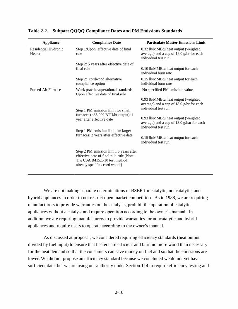
Table 2-2. Subpart QQQQ Compliance Dates and PM Emissions Standards
Appliance Compliance Date Particulate Matter Emissions Limit
Residential Hydronic
Heater
Step 1:Upon effective date of final
rule
Step 2: 5 years after effective date of
final rule
0.32 lb/MMBtu heat output (weighted
average) and a cap of 18.0 g/hr for each
individual test run
0.10 lb/MMBtu heat output for each
individual burn rate
Step 2: cordwood alternative
compliance option
0.15 lb/MMBtu heat output for each
individual burn rate
Forced-Air Furnace Work practice/operational standards:
Upon effective date of final rule
Step 1 PM emission limit for small
furnaces (<65,000 BTU/hr output): 1
year after effective date
Step 1 PM emission limit for larger
furnaces: 2 years after effective date
Step 2 PM emission limit: 5 years after
effective date of final rule rule [Note:
The CSA B415.1-10 test method
already specifies cord wood.]
No specified PM emission value
0.93 lb/MMBtu heat output (weighted
average) and a cap of 18.0 g/hr for each
individual test run
0.93 lb/MMBtu heat output (weighted
average) and a cap of 18.0 g/har for each
individual test run
0.15 lb/MMBtu heat output for each
individual test run
We are not making separate determinations of BSER for catalytic, noncatalytic, and
hybrid appliances in order to not restrict open market competition. As in 1988, we are requiring
manufacturers to provide warranties on the catalysts, prohibit the operation of catalytic
appliances without a catalyst and require operation according to the owner’s manual. In
addition, we are requiring manufacturers to provide warranties for noncatalytic and hybrid
appliances and require users to operate according to the owner’s manual.
As discussed at proposal, we considered requiring efficiency standards (heat output
divided by fuel input) to ensure that heaters are efficient and burn no more wood than necessary
for the heat demand so that the consumers can save money on fuel and so that the emissions are
lower. We did not propose an efficiency standard because we concluded we do not yet have
sufficient data, but we are using our authority under Section 114 to require efficiency testing and

2-11
reporting to the EPA. We will include this information on the EPA Burn Wise website. This will
help .
At this time, we lack sufficient data to issue a CO emissions limit in today’s final rule.
However, we are using our authority under Section 114 to require manufacturers to determine
CO emissions during the compliance tests (as typically conducted), report those results to the
EPA and include those results on the manufacturer’s website, so that data will be available to
consumers, and to the EPA and states for possible future rulemaking. We also plan to post
context and consumer-friendly summaries of the submitted data on the EPA Burn Wise website.
In this final rule, we are not setting limits on visible emissions, and we are not prohibiting
use in non-heating seasons. However, operators should note that some state, local and tribal
jurisdictions have specific limits, prohibitions and other requirements that must be followed.
Like the subpart AAA requirements, the subpart QQQQ requirements provide a retail
sell-through for hydronic heaters until December 31, 2015 so that retailers can sell their
inventory for the heating season of units manufactured before the compliance date. For forced-
air furnaces, the work practice/operational standards required on the effective date can be
promptly met so there is no need for a retail sell-through for those models
As in subpart AAA, subpart QQQQ includes a list of prohibited fuels because their use
would cause poor combustion or even hazardous conditions. Also, as in subpart AAA, subpart
QQQQ requires that the user must operate the hydronic heater or forced-air furnace in a manner
that is consistent with the owner’s manual. For pellet-fueled appliances, operation according to
the owner’s manual includes operation only with pellet fuels that are specified in the owner’s
manual or better. As in subpart AAA, manufacturers must only specify graded and licensed
pellets that meet certain minimum requirements or better. Data show that pellet quality is
important to ensure that the appliances operate properly such that emissions are within the
appliance certification limits.
The permanent labeling requirements and owner’s manual requirements in subpart
QQQQ are similar to the guidelines in the EPA’s current voluntary hydronic heater program with
some improvements. Like in subpart AAA, the temporary labels (voluntary hangtags) are only
for models that meet Step 2 levels before the compliance date and these voluntary hangtags end
upon the Step 2 compliance date. Subpart QQQQ also has a cord wood alternative compliance
option with a special permanent label and temporary label (voluntary hangtag) for models that

2-12
meet Step 2 using cord wood. The structure of the rest of subpart QQQQ is similar to the subpart
AAA certification and quality assurance process.
The final rule requires that before manufacture all affected hydronic heaters and forced-
air furnaces subject to new subpart QQQQ PM emission limits must conduct certification
compliance testing, submit a certificate of compliance and receive EPA approval for the PM
emission limits by the deadlines shown in Table 2-2.
The final rule requires testing of hydronic heaters by one of the following methods: EPA
Method 28 WHH, EPA Method 28 WHH- ASTM E2618-13, or EN 303--05 with certain
adjustments and conditions specified in the rule. As with all NSPS, affected sources may request
EPA approval of alternative test methods on a case-by-case basis as appropriate. See CAA Part
60, Subpart A, General Provisions at 60.8.
In this final rule, the EPA is relying on the cord wood test method that has been
developed by the CSA for forced-air furnaces. The current version of CSA B415.1-10 was
published in March 2010, and it includes not only the forced-air furnace test method but also
Canadian emission performance specifications for indoor and outdoor central heating appliances.
(The Step 1 PM emission level of 0.93 lb/MMBtu heat output is identical to the CSA B415.1-10
standard that was issued in 2010.) Also, in this final rule we are relying on efficiency test
methods that have been developed by the CSA.
2.4 Summary of Significant Changes to the Rule Following Proposal
2.4.1. Particulate Emission Standards
2.4.1.1. Room Heaters
The EPA is changing the proposed Step 2 PM emissions limit for new residential room
heaters, including catalytic and noncatalytic adjustable rate wood heaters, single burn rate wood
heaters or pellet heaters/stoves from 1.3 g/hr to 2.0 g/hr using crib wood. (Note that the
emissions standards are “as measured” by the test methods specified in the rule and labeled as
PM although the PM is essentially all direct PM2.5.) Compliance for room heaters will be
determined using the weighted average of burn rates rather than requiring each individual burn
rate to meet the limit. To reduce potential certification delays and unnecessary costs for small
businesses, we are adding automatic deeming of Step 1 certification for models with valid EPA
certifications under the 1988 NSPS that show that that the models achieve the Step 1 PM
emission levels. Manufacturers may choose to test using either crib wood or cord wood. Testing
with cord wood is not required for new residential room heaters under this final rule. If the

2-13
manufacturers voluntarily choose the cord wood alternative compliance option, the PM emission
limit for cord wood is 2.5 g/hr. Although the number is higher, the cord wood test method is
more reflective of fuel that is used in homes and the data available to the EPA indicate that this
emission level is at least as stringent as the 2.0 g/hr primary crib wood testing emission limit.
If the wood heater/stove manufacturer chooses to perform certification testing using cord
wood, the manufacturer may use a special EPA label for these certified models which
recognizes that cord wood testing more closely reflects actual in-home use.
The retail sell-through period has been extended from 6 months after the effective date to
December 31, 2015, to better cover the heating sales season.
2.4.1.2. Central Heaters: Hydronic Heaters and Forced-Air Furnaces
For new residential hydronic heaters and forced-air furnaces, the EPA is increasing the
proposed Step 1 emissions cap of 7.5 g/hr for any individual test run to 18.0 g/hr to match the
Phase 2 qualification levels in the EPA hydronic heater voluntary program. The final rule deems
hydronic heater models automatically certified to the Step 1 PM emission level if they are
qualified as meeting the Phase 2 emissions level under the EPA’s voluntary program. To reduce
potential certification delays and unnecessary costs for small businesses, we are also adding
automatic Step 1 certification for new hydronic heater models that have NYSDEC approval of
tests that demonstrate that the models achieve the Step 1 levels or are RHNY-qualified pellet
hydronic heaters. Similarly, we are adding automatic Step 1 certification for forced-air furnaces
that are certified under CSA B415.1-10 to meet the Step 1 PM emissions level.
We are changing the proposed hydronic heater Step 2 PM emissions limit of 0.06
lb/million BTU heat output for each burn rate to a final emissions limit of 0.10 lb/million BTU
heat output for each burn rate, tested on crib wood. Manufacturers may choose to test using
either crib wood or cord wood. If the manufacturer chooses the cord wood alternative
compliance option, the Step 2 PM emission limit for cord wood is 0.15 pounds per million BTU
heat output using cord wood. Although the number is higher, the cord wood test method is more
reflective of the fuel that is used in homes and the limited cord wood data available to the EPA
indicate that this emission level is at least as stringent as the 0.10 lb/million BTU heat output crib
wood testing emission limit. There is no crib wood Step 2 PM emission level for forced-air
furnaces because CSA B415.1-10 already specifies the use of cord wood test fuel.
If hydronic heater manufacturers and forced-air furnace manufacturers choose to test with
cord wood, they are allowed to use special permanent EPA labels and temporary EPA labels
2-14
(voluntary hangtags) for these certified models, which recognized that cord wood testing more
closely reflects actual operation under in-home-use conditions.
2.4.1.3. Masonry Heaters
As stated in section III of the preamble, the EPA is not taking final action on new
residential masonry heaters at this time. Comments indicated that the Masonry Heater
Association (MHA) needs more time to finish their efforts to develop revised test methods,
alternative compliance calculation procedures and dimensioning procedures. The MHA
comments stated that the cost of testing is high and impractical because almost all are custom-
built onsite. After we receive additional information from MHA and others, we will consider
taking final action for new residential masonry heaters in a future rulemaking.
The potential emission impact of this delay is small. Fewer than 1,000 masonry heaters
are built each year. Most manufacturers build fewer than 15 heaters per year. The total
nationwide annual emissions are estimated to be less than 10 tons of PM2.5.
2.4.2. Appliance Certification and Accreditation of Laboratories and Certifying Entities
In section III.D of the preamble to the proposed rule, we described the proposed approach
for a third-party certification program by an International Organization for Standardization
(ISO)-accredited certifying body and testing by ISO-accredited testing laboratories. This
approach requires manufacturers to use third-party, independent ISO-accredited and EPA-
approved test labs and certifying entities to demonstrate compliance with a representative
appliance for a model line.
Under the Administrator Approval Process (see section 60.533(c) of the proposed rule),
we proposed a transition period of 1 year from the effective date of the final rule for test labs to
receive ISO accreditation through an EPA-recognized accreditation body. In this final rule for
room heaters and central heaters, we are increasing the transition period for test laboratories that
are currently EPA-accredited from 1 year to 3 years from the effective date of this final rule. This
additional time for test laboratory accreditation will reduce concerns about costs for small labs
and potential testing delays.
We proposed that certifying entities be required to receive ISO accreditation upon the
effective date of the final rule; however, commenters stated that ISO accreditations can take 6
months. Requiring use of ISO-accredited certifying bodies/entities on the effective date of the
final rule can be difficult for small manufacturers of wood stoves/heaters and forced-air furnaces,
which previously have not been required to obtain certifications from ISO-accredited certifying

2-15
bodies/entities; therefore, we are allowing a 6-month transition for models other than hydronic
heaters. The 6-month transition period does not apply to hydronic heaters because they already
use ISO-accredited certifying bodies/entities for the EPA’s Voluntary Partnership Program.

3-1
SECTION 3
INDUSTRY PROFILE
The revisions to the NSPS for residential wood heaters would cover a number of devices
that include wood stoves/heaters, pellet stoves/heaters; indoor and outdoor hydronic heaters and
forced-air furnaces. (This RIA and the final rule use the terms stove, heater, and stove/heater
interchangeably.) EPA has developed this industry profile to provide the reader with a general
understanding of the technical and economic aspects of the industries that would be directly
affected by potential revisions to the NSPS regulation for new residential wood heaters and to
offer information relevant to preparing an economic impact analysis (EIA) for this revision to
the NSPS. We begin by outlining the supply side by discussing the production process for wood
heaters and the associated costs and follow this with an overview of the demand side of the
market for residential wood heaters as a primary or secondary home heating system. We then
address the characteristics that define the residential wood heating market and profile the
companies that produce wood heating systems. Although the wood heating equipment industry
includes multiple product markets, there is little published information about the intricacies of
each individual market. For this profile, we analyzed the wood heating market primarily on an
aggregated level and provide detailed information for specific product markets when such
information is available.
3.1 Supply Side
Wood heating devices embody a variety of products that provide heat for residential
consumers by burning wood or other solid biomass fuel. Indoor wood-burning devices can
provide space heating for a single room or can be central heaters for a residential home. Indoor
heating devices include freestanding wood stoves, pellet stoves, fireplace inserts, and forced-air
furnaces. Outdoor wood heating devices, also known as outdoor wood boilers, or water stoves,
are typically located adjacent to the home they heat in small sheds with short smoke stacks.
Other products considered in the development of revisions of this NSPS (but not included in this
rulemaking) include low-mass fireplaces, open masonry fireplaces, fireplaces, fire pits,
chimineas, cook stoves, masonry heaters, and pizza ovens Masonry heaters were included in the
proposed NSPS, but are not included in the final NSPS. The basis for the removal of masonry
heaters from this rule can be found in Section 2 of this RIA or the preamble to the final rule.
This section provides a general description of the residential wood heater manufacturing
processes. We then provide more detailed definitions of the indoor and outdoor wood heater
products considered and the wood fuels used in their operation.

3-2
3.1.1 Production Process
The manufacturing process for residential wood heaters varies depending on the product
type being produced. Generally, the manufacturing process entails the assembly of several
prefabricated metal components. Major inputs include cast iron, metal products, heat-proof glass,
fireproof fabric insulation, refractory brick, and heat-tolerant enamels or coatings.
Wood heating devices are typically categorized by emissions and efficiency ratings. The
emissions ratings typically use EPA, ASTM, CSA, or EN (European Union) test methods. The
efficiency ratings are based on tests that measure the amount of heating value transferred from a
full load of wood or other biomass fuel (fuel type varies based on the product being tested) to the
living space. Efficiency tests evaluate two performance metrics that include combustion and heat
transfer efficiency. Combustion efficiency determines how effective the fire box design is at
burning the fuel and extracting its heating value. Heat transfer efficiency tests are potentially
conducted in calorimeter rooms equipped with temperature sensors to measure the degree
changes in the heated living space and the flue exhaust to determine how much heat from the fire
is delivered to the living space compared with the heat lost up the flue (EPA, 2009c).
Thermal output, typically expressed in British thermal units per hour (BTU/hr) in the
United States, is the heat output measure that tells the amount of heat produced each hour. A
higher BTU/hr rate suggests that a stove will produce more heat per hour than a stove with a
lower rating. Depending on design and size characteristics, a space heating device heat output
rating ranges between 8,000 and 90,000 BTU/hr. Larger heating systems designed to provide
whole home heating have heat output ratings that range from 100,000 to greater than one million
BTU/hr.
3.1.2 Product Types
3.1.2.1 Wood and Coal Stoves
EPA-certified wood stoves typically are enclosed combustion devices that provide direct
space heating for a specific room or area of a home.4 Catalytic and noncatalytic wood stoves are
two general types of wood stoves available in the United States. (Some models are hybrids.) This
designation refers to the design of the combustion system. Noncatalytic combustion systems rely
on high temperatures (>1,000°F) within the fire box to fully combust the chemical compounds
(combustible gases and particles) in the wood smoke. In catalytic combustion systems, the
presence of the catalytic element lowers the temperature at which wood smoke chemical
4 EPA-certified wood stoves are those wood stoves that meet the requirements under the current residential wood
heater NSPS.
3-3
compounds combust. Catalytic elements or combustion system designs in noncatalytic
combustion systems are used in existing stoves to meet EPA emission standards.
Coal stoves are similar in structure and appearance to wood stoves. Most coal stoves are
designed to burn hard anthracite coal instead of soft bituminous coal (Houck, 2009), but different
varieties of coal have been used in coal stoves over time. Stoves that solely burn coal are not
affected by the revisions to the NSPS.
3.1.2.2 Wood Pellet Stoves and Biomass Stoves
Wood pellet and other biomass stoves are similar in application to wood stoves but
generate heat through pellet combustion. Wood pellet stoves use tightly compacted pellets of
wood as fuel, whereas other biomass stoves can use a variety of pellet types, including corn, fruit
pits, and cotton seed (EPA, 2009c). A load of pellets is poured into the stove’s hopper; then the
user sets a thermostat that controls a feed device within the stove. The feed device regulates the
amount of fuel that is released from the hopper into the heating chamber, which is where the
combustion takes place (EPA, 2009c). Pellet stoves are typically more efficient in terms of
combustion and heating than standard wood stoves but require electricity to operate the fans,
controls, and pellet feeders (EPA, 2009c). Stoves that solely burn non-wood biomass are not
affected by the revisions to the NSPS.
3.1.2.3 Masonry Heaters
A masonry heater is a solid-fueled heating device that is pre-manufactured or constructed
on site using mainly masonry or ceramic materials (Masonry Heater Association of North
America, 1998). Though masonry heaters and traditional fireplaces are similar in appearance,
masonry heaters are used primarily to generate heat, whereas fireplaces typically serve a more
aesthetic purpose. The heater itself is made up of an interior construction unit consisting of a
firebox and a set of heat exchange channels (Chernov, 2008). The hot gas produced during rapid
combustion of fuel within the firebox passes through the heat exchange channels, which run
throughout the structure and saturate the masonry mass with heat (Chernov, 2008). Most
masonry heaters weigh over 800 kg. After the masonry walls are saturated, the masonry heater
radiates the heat into the area for 12 to 15 hours (Chernov, 2008). Masonry heaters can heat a
home all day without having to burn continuously and are often used in areas where other fuel
sources are unavailable (Chernov, 2008). However, there is a significant lag time between the
initial burn and the time that the masonry structure releases sufficient heat to warm a living space
(U.S. Department of Energy [DOE], 2010). Masonry heaters were included in the proposal, but
are not affected by the final revisions to the NSPS. The rationale for the removal of masonry

3-4
heaters from the final rule can be found in Section 2 of the RIA and the preamble to the final
rule.
3.1.2.4 Fireplace Inserts
A fireplace insert is a type of heater/stove that is designed to fit inside the firebox of an
existing wood-burning fireplace (Wood Heat Organization, 2010). EPA-certified fireplace inserts
are essentially wood heaters/stoves without legs or pedestals. An insert is made of steel or cast
iron and is typically installed in masonry fireplaces or traditional fireplaces in order to provide
effective heating (Hearth, Patio, and Barbeque Association [HPBA], 2010b). As an insulated
closed-door system, a fireplace insert improves combustion by slowing down the fire, decreasing
the excess air, and increasing the fire’s temperature (HPBA, 2010b). In addition to wood-fueled
fireplace inserts, other inserts can be fueled with natural gas, propane, pellets, or coal (HPBA,
2010b).
Fireplace inserts are not covered under this NSPS.
3.1.2.5 Forced Air Furnaces
A forced-air furnace is a type of central heating system that typically burns cordwood or
pellets. A forced-air furnace is typically located inside a house and provides controlled heat
throughout a home using a network of air ducts (EPA, 2009c). This is a primary heating system
that requires electricity to operate and is much more common currently in the U.S. compared to
hydronic heaters.
3.1.2.6 Outdoor Wood Heaters
An outdoor wood heater, also often called a wood-fired boiler, is a type of hydronic
heater that is designed to be the home’s primary heating system. Wood boilers are typically
located outdoors and have the appearance of a small shed with a smokestack (EPA, 2009c).
Hydronic heaters burn wood to heat a working liquid contained in a closed-loop system. The
heated liquid is then circulated to the house to provide heat and hot water (EPA, 2009). Hydronic
heaters are typically sold in areas with cold climates where wood may be the most readily
available fuel source (EPA, 2009c). In addition to outdoor hydronic heaters, there is an emerging
market for indoor hydronic heaters. Currently, the indoor hydronic heater market is
approximately 10% of the hydronic heater market.
3.1.2.7 Indoor and Outdoor Fireplaces
Fireplaces are typically not effective heating sources and are typically considered more of
an aesthetic feature than a functional device. The common low-mass fireplace is pre-fabricated

3-5
of steel in a factory and shipped to the home builder. A low-mass fireplace and its attached
chimney are light enough to be weighed on a platform scale (EPA, 2009c). Although low-mass
fireplace installations in homes often surrounded by natural or synthetic facades of masonry–like
materials, they should not be confused with masonry fireplaces or masonry heaters that are
primarily constructed if brick, stone, or other masonry materials. Masonry fireplaces are
traditional, aesthetic fireplaces that do not have the extensive heat channels that define masonry
heaters (Fireplaces & Woodstoves, 2010).
Fireplaces are also often used to enhance the outdoor area of a house. A portable grated
cylinder style has a bottom basin surrounded by open grating for a fire, a cooking grate, and a lid
(EPA, 2009c). A permanent outdoor fireplace is similar to one that would be found indoors.
They can be freestanding or attached to the outside of the house (EPA, 2009c).
Indoor and outdoor fireplaces are not covered by or affected by the revisions to the
NSPS.
3.1.2.8 Fire Pits, Chimineas, Cook Stoves, and Pizza Ovens
Several outdoor appliances involve using wood fuel for cooking or heating. A fire pit is a
round outdoor hearth appliance that is designed to replicate the ambiance of a campfire by
radiating heat in 360 degrees around the pit (HPBA, 2010c). A chiminea is typically constructed
out of cast iron, terra cotta, or clay and burns firewood inside the internal oven. As the fire burns,
the walls of the oven absorb heat. After the dome chamber reaches the desired temperature, the
fire can be allowed to die down (EPA, 2009c). Wood cook stoves are made of cast iron to
withstand the high temperatures produced by the fire (EPA, 2009c). They are similar in
appearance to a conventional stove, complete with an oven and cooking ranges, but are larger in
order to accommodate the wood fuel (EPA, 2009c). North American traditional cook stoves have
defined dimensions and cooking performance characteristics. Native American bake ovens have
defined cultural and cooking functions. Pizza ovens are made out of a masonry material, such as
clay adobe or refractory bricks, which can endure high temperatures for an extended period of
time (EPA, 2009c).
These appliances are not covered or affected by the revisions to the NSPS.
3.1.3 Costs of Production
Because of the variety of products covered under the wood heat source category, different
manufacturers use a wide range of materials and have varying labor requirements. Since there is
significant diversity in output between the producers in this category, as well as the broader

3-6
industries in which they may be classified for data purposes, this section highlights the
production costs associated with several of the North American Industry Classification System
(NAICS) codes under which a significant number of the wood heating equipment manufacturing
facilities in our database are included.
Table 3-1 displays costs for the heating equipment and hardware manufacturing
industries. The production of devices like wood stoves, hydronic heaters, and fireplace inserts is
included under the heating equipment category (NAICS 333414). In 2011, the total cost of
materials used for production represented roughly 48% of the industry’s total value of shipments,
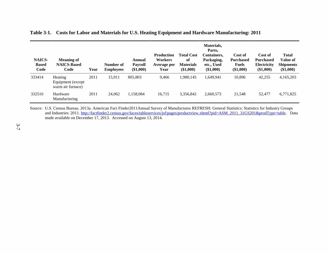
3-7
Table 3-1. Costs for Labor and Materials for U.S. Heating Equipment and Hardware Manufacturing: 2011
NAICS-
Based
Code
Meaning of
NAICS-Based
Code Year
Number of
Employees
Annual
Payroll
($1,000)
Production
Workers
Average per
Year
Total Cost
of
Materials
($1,000)
Materials,
Parts,
Containers,
Packaging,
etc., Used
($1,000)
Cost of
Purchased
Fuels
($1,000)
Cost of
Purchased
Electricity
($1,000)
Total
Value of
Shipments
($1,000)
333414 Heating
Equipment (except
warm air furnace)
2011 15,911 805,803 9,466 1,980,145 1,649,941 10,896 42,255 4,165,203
332510 Hardware
Manufacturing
2011 24,062 1,158,084 16,715 3,356,842 2,660,573 21,548 52,477 6,771,825
Source: U.S. Census Bureau. 2013a. American Fact Finder2011Annual Survey of Manufactures REFRESH: General Statistics: Statistics for Industry Groups
and Industries: 2011. http://factfinder2.census.gov/faces/tableservices/jsf/pages/productview.xhtml?pid=ASM_2011_31GS201&prodType=table. Data
made available on December 17, 2013. Accessed on August 13, 2014.

3-8
while labor costs (represented as annual payroll estimates) only represented 19%. The hardware
manufacturing industry (NAICS 332510) had fairly similar statistics: materials used and annual
payroll accounted for 50% and 17% of the total value of shipments, respectively.
The 2007 production costs for plumbing and heating equipment wholesalers (NAICS
423720), which are the most recent available from the Census Bureau, are outlined in Table 3-3.
This category includes the merchant wholesale production of cooking and heating stoves and
hydronic heaters. Table 3-4 displays the costs for certain home furnishing stores, including those
that sell wood stoves at retail prices. The costs for these industries may be more indicative of the
wholesale and retail exchanges of wood-heating equipment rather than the actual production
process.
3.2 Demand Side
The subject wood-fired heaters are sold explicitly for residential use. These devices can
be included in the original construction of a new home or installed later in the life of the home.
Demand for residential wood heating devices is driven by several key factors that include size,
price, efficiency, aesthetics, and fuel type (e.g., cord wood, pellet wood, or other biomass fuels).
However, consumer demand for any one product discussed in Section 3.1 is driven primarily by
the intended end-use heating application. This section defines the three major consumer
segments that drive demand based on the end-use application. Following this discussion, we
present some national statistics on the variation in residential wood heat consumers in the United
States. We conclude our discussion of the demand side by characterizing some of the substitutes
for residential wood-burning devices.

3-9
Table 3-2. Costs for U.S. Single-Family Home Contractors: 2007
NAICS-Based
Code
Meaning of NAICS-Based
Code Year Number of Employees Total Payroll ($1,000)
Cost of Materials,
Components, and
Supplies ($1,000)
Total Value of
Construction Work
($1,000)
236115 New single-family general
contractors
2007 259,905 10,834,064 37,676,878 89,282,708
Source: U.S. Census Bureau. 2010b. American Fact Finder. Sector 23: EC0723SG01: Construction: Summary Series: General Summary: Detailed Statistics for
Establishments: 2007. Released May 18, 2010. http://factfinder.census.gov.
Table 3-3. Costs for U.S. Plumbing and Heating Equipment Supplies Wholesalers: 2007
NAICS-Based
Code Meaning of NAICS-Based Code Year
Number of
Employees
Annual Payroll
($1,000)
423720 Plumbing and heating equipment
supplies (hydronics) merchant
wholesalers
2012 68,534 3,988,326
Source: U.S. Census Bureau, 2014c. American Fact Finder. 2012 County Business Patterns. Released June 26, 2014. Accessed on August 13, 2014.
http://factfinder2.census.gov/faces/tableservices/jsf/pages/productview.xhtml?pid=BP_2012_00A2&prodType=table
Table 3-4. Costs for U.S. Specialized Home Furnishing Stores: 2007
NAICS-Based
Code Meaning of NAICS-Based Code Year
Number of
Employees
Annual Payroll
($1,000)
442299 All other home furnishing stores 2012 14,731 2,780,875
Source: U.S. Census Bureau, 2014d. American Fact Finder. Sector 44: EC0744A1: Retail Trade: Geographic Area Series: Summary Statistics for the United
States, States, Metro Areas, Counties, and Places: 2012. Released on June 26, 2014. Accessed on August 13, 2014.
http://factfinder2.census.gov/faces/tableservices/jsf/pages/productview.xhtml?pid=BP_2012_00A1&prodType=table.
3-10
3.2.1 End-Use Consumer Segments
The intended end-use heating application is a primary driver of demand for residential
heating devices. The U.S. Annual Housing Survey (HUD, 2008) provides a starting point for
classifying the various types of residential consumer of heating equipment. For the purposes of
this profile we grouped consumers into three major segments based on their desired heating
needs: whole-house heating, secondary or zone heating, and recreational outdoor heating
applications.
The primary, or whole-house heating segment, includes homes with no other central
heating system that can provide heating service in or outside the house. In smaller homes, a large
stove or masonry heater may be sufficient to provide heat to the entire house. However, larger
homes typically require, either individually or in some combination thereof, an outdoor wood
boiler, a hydronic heater, or a pellet-burning forced-air furnace, to meet the consumers’ heating
needs.
The secondary, or zone heating segment, includes consumers that desire supplemental
heat from a wood-burning device in homes with an existing central heating system that serves as
the home’s primary heat source. Cordwood and wood pellet-burning stoves are ideal for heating
a single room or zone within a home. Smaller masonry heaters are also well suited for zone
heating needs.
Finally, a third component of demand is represented by consumers who desire a wood-
burning device for recreational aesthetic applications. Outdoor fireplaces, chimineas, outdoor
ovens, and pizza stoves are some examples of the wood-burning devices designed for
recreational applications. The products that address the needs of this consumer segment are
primarily intended to enhance the aesthetics or landscape outside the home. Indoor fireplaces
typically serve aesthetic or recreational purposes rather than providing effective room heat. Only
about 9% of wood fireplaces are used for heat generation (HPBA, 2010a).
3.2.2 Regional Variation in Residential Demand
In 2010, 2.1% of total occupied homes in the United States relied on wood heat as the
primary fuel source for home heating. The demand for wood heat is concentrated in the
Northeast, the Northwest, and the northern Midwest regions of the United States. Table 3-5

3-11
Table 3-5. Wood as Primary Fuel Source for Home Heating in the United States: 2006–
2008
State
Percentage of State Owner-
Occupied Houses
Percentage of National
Owner-Occupied Houses Count
California 2% 9% 165,440
New York 3% 6% 103,740
Pennsylvania 3% 6% 100,355
Washington 6% 5% 92,664
Michigan 3% 5% 85,712
Wisconsin 5% 5% 83,040
Oregon 8% 4% 79,637
Ohio 2% 4% 67,665
Virginia 3% 3% 60,579
North Carolina 2% 3% 58,397
Minnesota 3% 2% 43,234
Maine 10% 2% 41,509
Indiana 2% 2% 38,550
West Virginia 7% 2% 38,142
Idaho 8% 2% 32,817
Colorado 2% 2% 28,668
Vermont 15% 1% 26,601
Massachusetts 2% 1% 25,870
Montana 9% 1% 24,355
New Hampshire 7% 1% 24,071
Top 20 total 68% 1,221,046
National total 100% 1,792,741
Source: U.S. Census Bureau. 2009. American Community Survey: 2006–2008. Available at:
http://factfinder.census.gov/servlet/DatasetMainPageServlet?_program=ACS&_submenuId=&_lang=en&_
ts=.
illustrates this regional concentration by listing the 20 states that represent the highest percentage
of households that use wood heat based on Census data from 2006–2008. The second column
shows the number of wood-heat users as a percentage of the total homes in the state, while the
third column shows the number of wood-heated homes as a percentage of the total users in the
United States. These 20 states account for over two-thirds of the total primary U.S. residential
wood heat demand.

3-12
About 10–12% of American households use wood when secondary wood heat demand is
counted, according to the Census and the Energy Information Administration (EIA). Table 3-6
illustrates the regional breakdown of secondary wood heat demand by U.S. Census divisions in
2009, which is the most recent year for which these data are available. Roughly 8% of the
American households use wood as a secondary heat source.
Table 3-6. Wood as Secondary Heat Source by Census Division, 2009 (millions of
households)
Census Division Number of Households
Percentage of U.S.
Households using
Wood as Secondary
Heat Source
Percentage of Total
U.S. Households
Northeast 1.7 19% 2%
Midwest 1.9 22% 2%
South 2.6 30% 2%
West 2.5 28% 2%
Grand total 8.8 8%
Total U.S. households 113.6
Source: U.S. Energy Information Administration, 2013. Residential Energy Consumption Survey: 2009. Available
at. http://www.eia.gov/consumption/residential/data/2009/index.cfm#undefined. Released (final) April
2013.
Figure 3-1 shows which states fall into which Census divisions. More households rely on
wood fuel as a supplemental heat source rather than as a primary source. Roughly 8% of
American households used wood fuel for a secondary heat source in 2009, whereas 3% of
households relied on wood for their primary heat source in the same year. The proportion of the
population using primary wood heat was relatively consistent between 2005 data presented in
Table 3-6 and the 2006 to 2008 period, as shown in Table 3-5.4 One interesting note about
4 Although the total occupied households between the Department of Energy’s Residential Energy Consumption
Survey [RECS] and the Census Bureau’s American Community Survey [ACS] differ, the proportion of total
occupied households using wood fuel as their primary home heating fuel is consistent. The survey data sources
used in Table 3-6 assumes 111 million occupied homes in 2009 while Figure 2-2 assumes 109 million for the
same year.

3-13
Figure 3-1. Census Regions and Divisions of the United States
Source: U.S. Census Bureau, 2014e. Census Regions and Divisions of the United States. Available at
https://www.census.gov/geo/maps-data/maps/pdfs/reference/us_regdiv.pdf.
secondary wood fuel use is that it does not appear prevalent in the Middle Atlantic or New
England states, which account for only 19% of the total secondary use. This fact is in contrast to
the primary use data in Table 3-5, which shows households in Vermont, New Hampshire, Maine,
Pennsylvania, Massachusetts, and New York accounting for 17% of the total national primary
demand.
Within the wood heat demand constituency, there is also regional demand variation for
different wood-fueled appliances. For example, the demand for wood-fired forced-air furnaces is
concentrated primarily in the Great Lakes region of the country and, to a lesser extent, the
Midwest (HPBA, 2010a). These two regions account for 82% of the 30,000 to 35,000 furnaces
sold annually in the United States (HPBA, 2010a). Demand for wood-fueled cook stoves is
concentrated in the Amish and Mennonite communities in the Midwest (HPBA, 2010a).
3.2.3 National Home Heating Trends
Residential demand for wood fuel has been declining steadily throughout the United
States over a fairly long period of time. Figure 3-2 illustrates the number of households from
1989 to 2005 that reported using wood fuel for heating, cooking, or heating water. In 1989,
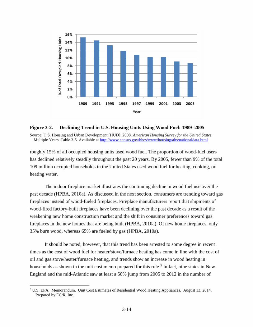
3-14
Figure 3-2. Declining Trend in U.S. Housing Units Using Wood Fuel: 1989–2005
Source: U.S. Housing and Urban Development [HUD]. 2008. American Housing Survey for the United States.
Multiple Years. Table 3-5. Available at http://www.census.gov/hhes/www/housing/ahs/nationaldata.html.
roughly 15% of all occupied housing units used wood fuel. The proportion of wood-fuel users
has declined relatively steadily throughout the past 20 years. By 2005, fewer than 9% of the total
109 million occupied households in the United States used wood fuel for heating, cooking, or
heating water.
The indoor fireplace market illustrates the continuing decline in wood fuel use over the
past decade (HPBA, 2010a). As discussed in the next section, consumers are trending toward gas
fireplaces instead of wood-fueled fireplaces. Fireplace manufacturers report that shipments of
wood-fired factory-built fireplaces have been declining over the past decade as a result of the
weakening new home construction market and the shift in consumer preferences toward gas
fireplaces in the new homes that are being built (HPBA, 2010a). Of new home fireplaces, only
35% burn wood, whereas 65% are fueled by gas (HPBA, 2010a).
It should be noted, however, that this trend has been arrested to some degree in recent
times as the cost of wood fuel for heater/stove/furnace heating has come in line with the cost of
oil and gas stove/heater/furnace heating, and trends show an increase in wood heating in
households as shown in the unit cost memo prepared for this rule.5 In fact, nine states in New
England and the mid-Atlantic saw at least a 50% jump from 2005 to 2012 in the number of
5 U.S. EPA. Memorandum. Unit Cost Estimates of Residential Wood Heating Appliances. August 13, 2014.
Prepared by EC/R, Inc.
0%
2%
4%
6%
8%
10%
12%
14%
16%
1989 1991 1993 1995 1997 1999 2001 2003 2005
% o
f To
tal
Occ
up
ied
Ho
usi
ng
Un
its
Year
3-15
households that rely on wood as the main heating source. As the use of fuel oil and kerosene in
this region has declined in recent years, many households have turned to lower-cost alternatives,
including wood. In total, about 2.5 million households (2.1%) across the country use wood as the
main fuel for home heating, up from 1.9 million households (1.7%) in 2005.6
3.2.4 Substitution Possibilities
The availability of close substitutes for wood heating equipment is largely contingent on
two key factors: (1) the consumer’s heating needs and preferences and (2) the price and
availability of an alternative heating source. As discussed in Section 3.2.1, consumers tend to fall
into one of three demand segments depending on their desired end use for their heating device.
Each consumer group displays varying degrees of substitutability. The relative price of
alternatives is also an important aspect of product substitution, which includes the cost of the
heating equipment itself and the price and availability of the fuel it requires.
For most consumers looking for whole-house heat or single-room heat, gas or electric
heat provides a common substitute for wood fuel. Electricity can power central heating systems
for whole-house heat and smaller space heaters for single rooms. Since the majority of American
households have easy access to electric power, these home heating options are often a convenient
and low-cost alternative to wood heat. Gas-powered central furnaces and room heaters and oil-
powered central heating systems are also on the market for residential use (DOE, 2009).
Although most consumers have homes equipped for gas or electric power, more rural areas of the
country have limited access to reliable utilities. In these regions, electric or gas heat may not be
an available or cost-efficient choice relative to wood heat.
Recreational or aesthetic wood-fired appliances have fewer direct substitutes. Traditional
indoor fireplaces and masonry fireplaces can be outfitted for burning natural gas rather than
wood. Consumers may have a personal preference for one over the other. Wood fuel can be
messy and somewhat difficult to store, whereas natural gas can be more convenient and easier to
use, and gas furnaces can be much more efficient. Outdoor recreational appliances may be
difficult to substitute directly because many consumers desire the aesthetic effect created by a
wood-burning fire pit or chiminea. Outdoor charcoal or gas grills provide an alternative for
outdoor wood-fired cooking appliances, but consumers may not consider these a direct
6 U.S. Energy Information Administration. “Increase in wood as main source of house heating most notable in the
Northeast.” Released on March 17, 2014. Available at http://www.eia.gov/todayinenergy/detail.cfm?id=15431.

3-16
substitute. It should be noted that outdoor recreational wood-burning appliances such as fire pits,
chiminea, and grills are not covered in this final rule.
3.2.5 Price Elasticity of Demand
Price elasticity of demand is a concept in economic theory. It is a numeric measure of the
sensitivity of quantity demanded following an increase or decrease in the product’s price. The
level of sensitivity is determined by a number of factors that include the availability and price of
substitutes (e.g., other types of heating equipment, gas or electric space heaters and furnaces) and
the price of complements (wood fuels). A study done on residential wood energy consumption
from 1967 to 2009 showed that a composite of non-wood energy prices was positively associated
with U.S. residential wood energy consumption in the long-run with elasticity of 1.82. This can
be interpreted as a 1% increase in non-wood energy prices leading to a 1.82% increase in U.S.
residential wood energy consumption.7
In preparing this profile, we searched for, but were unable to identify, any empirical
estimates of the price elasticity of demand for residential wood heating equipment in recent
times. An estimate, which is now dated, of −1.6 was derived for use in the RIA for the 1988
Residential Wood Combustion NSPS (EPA, 1986). A commenter on the proposed NSPS
estimated a price elasticity of demand for hydronic heaters of -1.0 based on data taken from sales
trends in states with hydronic heater standards.8 We do not have elasticities for the other
appliances covered in this final rule. Although numerous articles estimate the elasticity of
demand for residential energy and heating fuels, these estimates focus almost exclusively on
electricity, natural gas, and fuel oil. These estimates find that residential energy and heating fuel
demand is relatively inelastic (i.e., there are only very small changes in demand in response to an
increase in energy or fuel prices). A recent RAND report suggests that in the short term, demand
for electricity and natural gas in residential markets is relatively inelastic (Bernstein and Griffin,
2005). However, the authors of the report also note that sustained higher energy prices in the
long term may result in demand for energy becoming more elastic as consumers have time to
identify more energy-efficient options.
With limited empirical estimates, we offer a qualitative discussion of the key
determinants of the price elasticity of demand to provide a general sense of whether consumer
7 Song. N. Aguilar, F.X., Shiftley. S.R., and Goerndt, M. Analysis of U.S. Residential Wood Energy Consumption:
1967-2009. Energy Economics, 34(6). November 2012. Pp. 2116-2124. 8 NERA. Cost-Effectiveness Analysis of Alternative Hydronic Heater New Source Performance Standards. May
2014. Prepared for the Hearth, Patio, and Barbecue Association.

3-17
demand is elastic or inelastic. As mentioned earlier, the determinants of elasticity include the
degree of substitutability, product necessity, and duration of the price increase.
There are a number of close substitutes for residential wood heating devices that include
electric and gas furnaces and space heaters. The extent to which consumers are able to substitute
between these options is likely to vary depending on geographic location. Overall, the presence
of good substitutes will increase the elasticity of demand for wood heating equipment. In
contrast, if locally-available alternative heating fuels (i.e., electricity, and fuel oil) are relatively
higher priced, it may make switching away from wood heating equipment less likely and,
ultimately, make demand for wood heating equipment inelastic. Also, the elasticity may depend
on whether the fuel in question is a secondary source of fuel instead of a primary fuel source.
Finally, the magnitude of the cost for residential wood heating equipment may also
increase the elasticity of demand. Consumer demand tends to be more elastic when the price of
the good represents a large proportion of consumer income (Bernstein and Griffin, 2005). In
other words, consumers become more sensitive to small price changes when considering the
purchase of a large household appliance (e.g., refrigerator, oven range, or heating system).
3.3 Industry Organization
A review and description of market characteristics (i.e., geography, product
differentiation, product transportation, entry barriers, and degree of concentration) can enhance
our understanding of the mechanisms underlying the wood heating equipment industry. These
characteristics provide indicators of a firm’s ability to influence market prices by varying the
quantity of product it sells. For example, in markets with large numbers of sellers and identical
products, firms are unlikely to be able to influence market prices via their production decisions
(i.e., they are “price takers” and operate in highly competitive markets). However, in markets
with few firms, significant barriers to entry (e.g., licenses, legal restrictions, or high fixed costs),
or products that are similar but can be differentiated, a firm may have some degree of market
power (i.e., to set or significantly influence market prices). In addition, if a product is difficult to
transport over long distance (due to weight or hazardous nature), then the market size may be
more restricted than one might expect, all other things being equal.
3.3.1 Market Structure
Market structure characterizes the level of competition and determines the extent to
which producers and sellers can influence market prices. Economic market structure typically
focuses on the number of producers and consumers, the barriers to market entry, and product
substitutability.

3-18
The residential wood heater market contains a number of large producers selling a
number of differentiated products along with a large number of small producers. These
characteristics suggest a quasi-monopolistic competitive market (i.e., somewhere between highly
competitive and less competitive) for large producers who will have some influence over market
prices. For small producers, the market will be highly competitive in nature. In addition, existing
regulatory requirements for product testing and certifications represent a barrier to market entry
for new producers of wood heating devices. Competition in this market may be further
constrained by transportation costs due to the weight of these products. A similar assessment was
determined in the 1986 study by the American Enterprise Institute (AEI) and Brookings
Institution Joint Center for Regulatory Studies.
The AEI-Brookings report also identified several key factors that influence
manufacturers’ pricing decisions. These factors included production costs, prices of similar
products sold by competitors, transportation costs, combustion technology and efficiency, and
consumers’ ability to differentiate products based on brand name and efficiency.
Price elasticity of supply is a numeric measure of the industry’s response to a small
percentage increase in the product price (Landsburg, 2005). The law of supply suggests
producers supply greater quantities at higher prices as a result of increasing marginal returns for
each additional unit produced as the average cost per unit of output declines. As a result, the
elasticity of supply for most industries is positive. Determinants of supply elasticity are
flexibility of sellers to adjust production and the time period being considered in estimating the
elasticity. Most manufactured goods have an elastic supply, meaning that sellers can adjust
production quickly in response to a change in prices (Mankiw, 1998). Industries with excess
plant capacity are likely to have elastic supply as sellers can ramp up production in a relatively
short time frame.
Based on 2006 plant capacity utilization data as shown in Figure 3-3, the heating
equipment manufacturing industry averaged 60% utilization, growing from 59% in 2002 to a
maximum utilization of 65% in 2005 and then falling to 54% in 2006 (U.S. Census Bureau,
2007). Similar statistics are not available for more recent years because this survey was
discontinued after 2006. The available data suggest that there is ample existing capacity to
increase production in the short and long terms, assuming an increase in price of residential
wood-burning heating equipment.
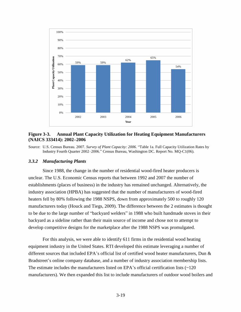
3-19
Figure 3-3. Annual Plant Capacity Utilization for Heating Equipment Manufacturers
(NAICS 333414): 2002–2006
Source: U.S. Census Bureau. 2007. Survey of Plant Capacity: 2006. “Table 1a. Full Capacity Utilization Rates by
Industry Fourth Quarter 2002–2006.” Census Bureau, Washington DC. Report No. MQ-C1(06).
3.3.2 Manufacturing Plants
Since 1988, the change in the number of residential wood-fired heater producers is
unclear. The U.S. Economic Census reports that between 1992 and 2007 the number of
establishments (places of business) in the industry has remained unchanged. Alternatively, the
industry association (HPBA) has suggested that the number of manufacturers of wood-fired
heaters fell by 80% following the 1988 NSPS, down from approximately 500 to roughly 120
manufacturers today (Houck and Tiegs, 2009). The difference between the 2 estimates is thought
to be due to the large number of “backyard welders” in 1988 who built handmade stoves in their
backyard as a sideline rather than their main source of income and chose not to attempt to
develop competitive designs for the marketplace after the 1988 NSPS was promulgated.
For this analysis, we were able to identify 611 firms in the residential wood heating
equipment industry in the United States. RTI developed this estimate leveraging a number of
different sources that included EPA’s official list of certified wood heater manufacturers, Dun &
Bradstreet’s online company database, and a number of industry association membership lists.
The estimate includes the manufacturers listed on EPA’s official certification lists (~120
manufacturers). We then expanded this list to include manufacturers of outdoor wood boilers and
59% 59%62%
65%
54%
0%
10%
20%
30%
40%
50%
60%
70%
80%
90%
100%
2002 2003 2004 2005 2006
Pla
nt C
ap
aci
ty U
tili
zati
on
Year

3-20
manufacturers of non-heating devices, such as cook stoves, outdoor fireplaces, and bake ovens.
Table 3-7 reports the count of U.S.-based companies in the industry by major business type.
Table 3-7. Number of U.S. Companies by Business Type
Business Type Number of Companies
Reported Sales 2008
($1,000s)
U.S. Market Share
(% of Net Sales)
Manufacturers 577 $1,285,800 97.00%
Wholesalers, distributors 19 $34,200 2.58%
Residential construction 10 $3,200 0.24%
Retailers 5 $600 0.04%
U.S. Totals 611 $1,324,000 100%
Sources: Dun & Bradstreet Marketplace, a company database. RTI International calculations.
Residential wood heater manufacturers account for over 90% of the firms in the industry
and span 14 different NAICS codes, of which 560 are categorized as NAICS 333414, as
establishments primarily engaged in manufacturing heating equipment (except electric and warm
air furnaces), such as heating boilers, heating stoves, floor and wall furnaces, and wall and
baseboard heating units (Census Bureau, 2010f). An average manufacturer may produce
anywhere from one to five technically different products (HPBA, 2010a). Manufacturers
dominate the market, accounting for over 97% of sales for the industry in 2008.
3.3.3 Location
The industry is, for the most part, co-located in areas of the country with the largest
demand for winter heating. Over 50% of U.S.-owned companies are located in 10 states in the
northern half of the country. The largest number of companies is located in California, with
additional concentrations in the Northwest, Northeast, the upper Midwest, and Central Plains.
Table 3-8 reports the number of U.S. companies for the top 10 states. Additionally,
approximately 104 foreign-based companies operate in the United States, two-thirds of which are
Canadian-based companies.

3-21
Table 3-8. U.S. Wood Heat Equipment Industry by Geographic Location
Location Business Count % of Total U.S. Industry
California 63 10%
Pennsylvania 36 6%
Minnesota 35 6%
New York 33 5%
Washington 31 5%
Ohio 29 5%
Texas 29 5%
Wisconsin 26 4%
Michigan 25 4%
Illinois 21 3%
U.S. Total 635 86%
Canada 67 9%
Other foreign 37 5%
Industry Total 739 100%
Sources: Dun & Bradstreet Marketplace, a company database. RTI International calculations.
3.3.4 Company Sales and Employment
Overall sales for the residential wood heating industry totaled more than $1.3 billion in
2008. Based on company data obtained for this profile, the industry employs approximately
17,000 workers annually. Previous analysis suggests that the industry relies on seasonal labor,
ramping up production in months leading up to winter and reducing employment and production
during the warmer parts of the year (AEI, 1986). Table 3-9 presents median sales and
employment for the industry by business type.

3-22
Table 3-9. U.S. Sales and Employment Statistics by Business Type
Business Type Number of Companies
Median Sales 2013
($1,000s)
Median Employment
per Company
Manufacturers 577 $219 4
Wholesalers, distributors 19 $548 5
Residential construction 10 $110 2
Retailers 5 $110 2
U.S. Totals 611 $247 4
Sources: Dun & Bradstreet Marketplace, a company database. RTI International calculations. Median sales estimates
are escalated to 2013 from 2008 using the GDP implicit price deflator. The resulting escalation ratio for
these years is 1.075. Annual values of the GDP implicit price deflator are available at
http://research.stlouisfed.org/fred2/series/GDPDEF/downloaddata.
Firms manufacturing heating equipment (except electric and warm air furnaces), such as
heating boilers, heating stoves, floor and wall furnaces, and wall and baseboard heating units
(NAICS 333414), are classified as small businesses by the Small Business Administration (SBA,
2014) if they have fewer than 500 employees. Looking across the manufacturing-related NAICS
codes in our analysis, we find that approximately 90% of manufacturers are considered small
businesses based on their reported employment compared with the SBA threshold. SBA
classifies wholesalers and distributors as small if their employment is fewer than 100 workers.
Approximately 68% of the industry’s wholesalers and distributors are considered small based on
the employment data obtained for this analysis.
SBA thresholds for construction, and retail firms are based on annual sales. SBA
standards for NAICS codes under these business types range between $20.5 and $33 million in
annual revenue. As reported in Table 3-9, median sales in these business categories are far below
the range of SBA standards. As one would expect, our analysis finds that all 39 firms are
considered small based on their reported annual sales compared with the SBA standards for their
respective NAICS code classifications.
3.3.4.1 Profits of Affected Entities
Table 3-10 reports profit margins for manufacturers, and wholesalers and distributors.
The profit margin represents an average of reported profit per unit sales across the industry
classified by the 6-digit NAICS code.

3-23
Table 3-10. Profit Margins for NAICS 333414 and 423720: 2008
NAICS
Code NAICS Description
Profit
Margin
Industry
Sales
($106)
333414 Heating Equipment Manufacturers 4.3% $70,965
423720 Plumbing and Heating Equipment Supplies (Hydronics) Merchant Wholesalers 3.4% $58,907
Source: The Risk Management Association. 2008. Annual Statement Studies, Financial Ratio Benchmarks 2008–
2009. Risk Management Association, Philadelphia: 2008.
3.4 Residential Wood Heater Market
Residential wood heating device shipments in the United States were relatively consistent
from year to year between 1998 and 2005, according to the HPBA’s reported hearth industry
shipment data (2009). Since 2005, total industry shipments on average have declined annually by
24%. Industry experts attribute this decline in large part to the broader economic downturn and
poor housing market. Renewable energy tax rebates offered in 2008 provided some relief for
pellet-fueled devices, resulting in a 1-year increase in shipments of 161%, only to steeply decline
again in 2009. This reflects the impact that the renewable energy tax rebates can have on wood
burning appliances depending on the size and duration of the rebates. Table 3-11 presents
shipment volumes by product type in 2008.
Outdoor wood boilers (or hydronic heaters) are a relatively new product in the market
since 1990. Previous studies have reported annual growth in sales of between 30 and 128%, with
over 155,000 outdoor wood boilers in use in the United States in 2006 (NESCAUM, 2006). Sales
have been regionally focused in the Northeast (especially the Great Lakes region) and
Midwestern states. The NESCAUM report predicted that over 500,000 outdoor wood boilers will
be in use before the end of 2010 if trends in annual sales continue to follow growth rates
observed between 1990 and 2006.
Market data for coal-burning stoves are very limited. However, anecdotal evidence
suggests that coal stove use is limited to major coal states, including Pennsylvania, West
Virginia, and Indiana, where coal is abundant and cheap relative to other heating fuels (Dagan,
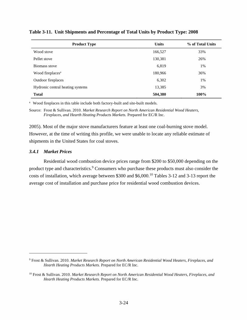
3-24
Table 3-11. Unit Shipments and Percentage of Total Units by Product Type: 2008
Product Type Units % of Total Units
Wood stove 166,527 33%
Pellet stove 130,381 26%
Biomass stove 6,819 1%
Wood fireplacesa 180,966 36%
Outdoor fireplaces 6,302 1%
Hydronic central heating systems 13,385 3%
Total 504,380 100%
a Wood fireplaces in this table include both factory-built and site-built models.
Source: Frost & Sullivan. 2010. Market Research Report on North American Residential Wood Heaters,
Fireplaces, and Hearth Heating Products Markets. Prepared for EC/R Inc.
2005). Most of the major stove manufacturers feature at least one coal-burning stove model.
However, at the time of writing this profile, we were unable to locate any reliable estimate of
shipments in the United States for coal stoves.
3.4.1 Market Prices
Residential wood combustion device prices range from $200 to $50,000 depending on the
product type and characteristics.9 Consumers who purchase these products must also consider the
costs of installation, which average between $300 and $6,000.10 Tables 3-12 and 3-13 report the
average cost of installation and purchase price for residential wood combustion devices.
9 Frost & Sullivan. 2010. Market Research Report on North American Residential Wood Heaters, Fireplaces, and
Hearth Heating Products Markets. Prepared for EC/R Inc.
10 Frost & Sullivan. 2010. Market Research Report on North American Residential Wood Heaters, Fireplaces, and
Hearth Heating Products Markets. Prepared for EC/R Inc.

3-25
Table 3-12. Installation Costs for Average System by Product Type (North America): 2008
Product Type Installation Cost
Wood stove $500
Pellet stove $300
Biomass stove $300
Wood fireplaces $600
Outdoor fireplaces $350
Hydronic central heating systems $2,000
Source: Frost & Sullivan. 2010. Market Research Report on North American Residential Wood Heaters,
Fireplaces, and Hearth Heating Products Markets. Prepared for EC/R Inc.
Table 3-13. Manufacturers’ Price by Product Type (North America): 2008
Product Type Average Price Price Range
Wood stove $848 $200 to $2,800
Pellet stove $1,279 $300 to $3,500
Biomass stove $1,403 $350 to $4,000
Wood fireplaces $450 $150 to $5,000
Outdoor fireplaces $755 $250 to $6,000
Hydronic central heating systems $7,433 $5,000 to $35,000
Source: Frost & Sullivan. 2010. Market Research Report on North American Residential Wood Heaters,
Fireplaces, and Hearth Heating Products Markets, Figure 2.6. Prepared for EC/R Inc.
Hydronic heaters are the most expensive product in Table 3-13 partly because of the
additional material requirements. The price of freestanding stoves and fireplace inserts varies
depending on the fuel it burns. Biomass stoves are almost twice as expensive as cord wood-
burning stoves because biomass stoves are more similar in construction to pellet stoves.
Although no price data exist on coal-burning stoves, costs are comparable to traditional cord
wood stoves. Coal stove prices for 2010 collected for this profile averaged $1,338 and ranged
between $500 and $3,000 depending on the size and manufacturer.
3.4.2 International Competition
The U.S. market for wood-fueled heating products has been concentrated on the local
scale in recent years. Manufacturers concentrate production where wood heat is in demand,
which is in the Northeast and Northwest. Some regions of the country have specific emissions
requirements on wood burning, so consumers may be restricted to buying stoves and heaters that
can cater to local regulations (Frost & Sullivan, 2010). Domestic producers have traditionally

3-26
faced some competition from European manufacturers in certain wood heat markets, but Asian
manufacturers have been gaining market share, especially in the EPA-certified wood stove and
currently exempt single-burn-rate stove markets (Frost & Sullivan, 2010).
Asian-based companies, especially those in China, have the advantage of relatively low
overhead and labor costs compared with other companies worldwide (Frost & Sullivan, 2010).
Although the products coming from these producers are lower in price, they are also lower in
quality (Frost & Sullivan, 2010). However, money-conscious consumers have been willing to
settle for lower quality stoves as the economy remains uncertain (Frost & Sullivan, 2010).
Companies from all over the world have been moving some manufacturing operations to China
in an attempt to compete with Asian producers through low-cost production (Frost & Sullivan,
2010). Still, U.S. manufacturers are likely to see increased competition from Asia in the future.
3.4.3 Future Market Trends
While there has been a steady decline in the residential markets for wood heaters,
fireplaces, and hearth products, increases in oil and gas prices have led to substitution back to
wood as a source of heat in 2007, in which a growth rate of 16.4% between 2007 and 2008 took
place in these markets. However, demand for these products fell victim to the recession in 2009
(Frost & Sullivan, 2010). A weak residential construction market coupled with a tight credit
market decreased overall demand in the market for wood heating products, which led analysts to
project a 2009 growth rate of −36.1% (Frost & Sullivan, 2010). The growth forecast for 2010
improved relative to 2009 to a rate of −4.1%, due in part to the residual effects of the severe
2009 winter temperatures and the financial incentive provided by the federal energy efficient tax
credit (Frost & Sullivan, 2010).
As the economy continues to recover beyond 2010, demand should trend upward as
consumers look to cut heating costs with wood and biomass (Frost & Sullivan, 2010). New home
construction and increased credit availability will further foster demand, which is expected to
grow at a compound annual rate of 4.1% from 2009 to 2015 (Frost & Sullivan, 2010). The
current regional demand patterns are expected to continue, with the Northeast and Northwest
regions of the country driving wood fuel combustion demand, but analysts anticipate that the
wood heat product market will be embraced in other areas of the country in which wood and
biomass are viable and inexpensive fuel sources (Frost & Sullivan, 2010).
Although the overall residential wood heat market is expected to grow, there may be
variation in demand between individual product segments. Pellet and biomass stoves are
expected to lead the way in demand as consumers look for options with sustainable fuel sources

3-27
and cleaner-burning technologies (Frost & Sullivan, 2010). Outdoor wood boilers (hydronic
heaters) saw a surge in demand throughout the 1990s and mid-2000s, a trend that is projected to
continue (Northeast States for Coordinated Air Use Management, 2006). Future demand for
primary and secondary wood-burning heating devices will be somewhat dependent on the price
of wood fuel relative to electric and gas heat, as well as consumer preferences. Since fireplaces
and masonry fireplaces typically are not effective heaters and purchases are based on the
aesthetic value rather than function, future demand will likely stay in line with consumer
preferences.

4-1
SECTION 4
BASELINE EMISSIONS AND EMISSION REDUCTIONS
4.1 Introduction
This section presents the baseline emissions for the pollutants emitted by affected units
and also the resulting emissions after imposition of the NSPS. We present the baseline emissions
and emission reductions for PM2.5 and also for other pollutants from affected units such as
volatile organic compounds (VOCs) and carbon monoxide (CO). Baseline emissions were
calculated using a 2008 base inventory and were then projected to future years beyond the
promulgation of the rule in 2015 to 2020 and beyond, using emissions factors specific to the
category of the affected unit (e.g., certified wood stove, pellet stove). These emissions factors are
listed in the emissions memorandum for this final rule (EC/R, Inc., January 2015). Emission
reductions were calculated from the baseline emissions based on the considered emissions limits
for each appliance type affected, and the emission reductions were used as inputs to the benefits
analysis presented in Section 7.
4.2 Background to Emissions Estimates
We used the EPA Residential Wood Combustion (RWC) emission estimation tool,12
which is an AccessTM database that compiles nationwide RWC emissions using county level,
process specific data and calculations. We summed the nationwide number of appliances and
total tons of wood burned for each of the relevant product categories (Table 4-1 below) in the
inventory.
Table 4-1. RWC Emission Inventory Categories Used
Woodstove: fireplace inserts; EPA certified; non-catalytic
Woodstove: fireplace inserts; EPA certified; catalytic
Woodstove: freestanding, EPA certified, non-catalytic
Woodstove: freestanding, EPA certified, catalytic
Woodstove: pellet-fired, general
Woodstove: freestanding, non-EPA certified
Hydronic heater: outdoor
Furnaces: indoor, cordwood
12 rwc_2008_tToolv4.1_feb09_2010.zip.

4-2
We then made some adjustments/assumptions to the baseline RWC inventory. First, we
deleted data in the RWC database for non-certified stoves and inserts, as these cannot be sold.
With the exception of wood stoves, we applied the PM2.5 emission factors for each class to the
total tons of wood burned and calculated an average emission rate/appliance/category. In the case
of wood stoves, the RWC database used an average of all PM10 AP-42 emission factors for wood
stoves.13 The RWC database assumes that PM10 and PM2.5 factors are identical. At a minimum,
we estimate that all new wood stoves meet the AP-42 PM10 emission factors for “Phase II”
stoves (the current NSPS promulgated in 1988) and therefore started with the lower AP-42 Phase
II emissions factors for catalytic and non-catalytic stoves at baseline, rather than the higher
average of all AP-42 emission factors used in the RWC database. Furthermore, to avoid any
potential for overstating baseline emissions, we went a step further and assumed that all new
shipments will meet the current Washington State limits, which are approximately 40% less than
the 1988 NSPS Phase II limits. We therefore used baseline emission factors which are 60 percent
of the AP-42 Phase II emission factors – less than half the value used in the RWC to represent
the average of all AP-42 emission factors – in order to ensure a forward-looking and understated
baseline.
Second, we assumed that outdoor hydronic heaters and indoor hydronic heaters have the
same emission profile.
It should be noted that the PM2.5 emissions factors for hydronic heaters and cord wood
furnaces (i.e., forced air furnaces) increased to 64.0 lb/ton from the estimate of 27.6 lb/ton of
wood burned used for the proposal. The increase is a result of updates taken from a peer-
reviewed 2012 report14 that were applied in the RWC database These updates result from testing
of hydronic heater models that showed that PM2.5 emissions from these sources had been
underestimated at proposal. In addition, industry estimates of hydronic heater shipments were
higher than EPA’s estimates at proposal for particular years, and EPA has incorporated these
industry estimates into the shipment estimates used for emissions estimation in the final rule.
The PM2.5 emissions factors for the other appliance categories remain unchanged from the
proposal.
13 AP-42, Chapter 1.10, Residential Wood Stoves, Table 1.10-1. See:
http://www.epa.gov/ttnchie1/ap42/ch01/final/c01s10.pdf. 14 Emission factors for the final rule estimates are based on EPA's Residential Wood Combustion Tool version 4.1
with updates from the 2012 EPA report (Gullett et al., Environmental, Energy Market, and Health
Characterization of Wood-Fired Hydronic Heater, Final Report, June 2012).
4-3
Single burn rate stoves are not included in the RWC database as separate identifiable
units. We assumed that they would have the same baseline emission factor as freestanding non-
certified woodstoves, i.e., 30.6 lb/ton of wood burned. We used the average tons burned per
appliance factor as representative of these stoves as well.
We used this subset of the RWC database to calculate a baseline average emission
rate/appliance/category, including an adjustment of the RWC emission factor to the current
Washington State limits where warranted. We multiplied the total tons of wood burned for the
appliance by the RWC emission factor (adjusted as appropriate) to calculate the total tons of
PM2.5 emissions. We divided this value by the number of appliances in the category to calculate
the baseline average PM2.5 emissions per individual appliance, and these results are shown in
Table 4-2.
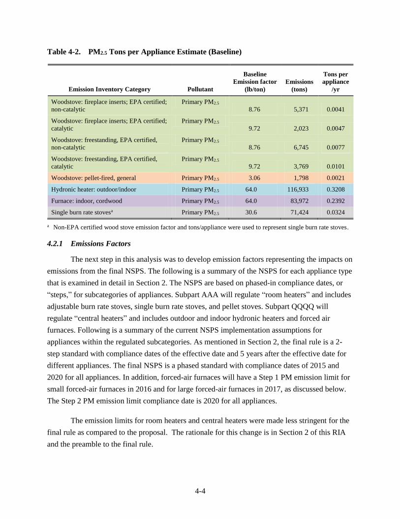
4-4
Table 4-2. PM2.5 Tons per Appliance Estimate (Baseline)
Emission Inventory Category Pollutant
Baseline
Emission factor
(lb/ton)
Emissions
(tons)
Tons per
appliance
/yr
Woodstove: fireplace inserts; EPA certified;
non-catalytic
Primary PM2.5
8.76 5,371 0.0041
Woodstove: fireplace inserts; EPA certified;
catalytic
Primary PM2.5
9.72 2,023 0.0047
Woodstove: freestanding, EPA certified,
non-catalytic
Primary PM2.5
8.76 6,745 0.0077
Woodstove: freestanding, EPA certified,
catalytic
Primary PM2.5
9.72 3,769 0.0101
Woodstove: pellet-fired, general Primary PM2.5 3.06 1,798 0.0021
Hydronic heater: outdoor/indoor Primary PM2.5 64.0 116,933 0.3208
Furnace: indoor, cordwood Primary PM2.5 64.0 83,972 0.2392
Single burn rate stovesa Primary PM2.5 30.6 71,424 0.0324
a Non-EPA certified wood stove emission factor and tons/appliance were used to represent single burn rate stoves.
4.2.1 Emissions Factors
The next step in this analysis was to develop emission factors representing the impacts on
emissions from the final NSPS. The following is a summary of the NSPS for each appliance type
that is examined in detail in Section 2. The NSPS are based on phased-in compliance dates, or
“steps,” for subcategories of appliances. Subpart AAA will regulate “room heaters” and includes
adjustable burn rate stoves, single burn rate stoves, and pellet stoves. Subpart QQQQ will
regulate “central heaters” and includes outdoor and indoor hydronic heaters and forced air
furnaces. Following is a summary of the current NSPS implementation assumptions for
appliances within the regulated subcategories. As mentioned in Section 2, the final rule is a 2-
step standard with compliance dates of the effective date and 5 years after the effective date for
different appliances. The final NSPS is a phased standard with compliance dates of 2015 and
2020 for all appliances. In addition, forced-air furnaces will have a Step 1 PM emission limit for
small forced-air furnaces in 2016 and for large forced-air furnaces in 2017, as discussed below.
The Step 2 PM emission limit compliance date is 2020 for all appliances.
The emission limits for room heaters and central heaters were made less stringent for the
final rule as compared to the proposal. The rationale for this change is in Section 2 of this RIA
and the preamble to the final rule.
4-5
Subpart AAA (“room heaters”):
These are adjustable burn rate, single burn rate, and pellet stoves: Step 1 PM
emissions limit of 4.5 g/hr upon promulgation in 2015; and Step 2 PM emissions limit
of 2.0 g/hr five years after promulgation in 2020. Note: The Step 1 limit is the 1995
Washington State standard for non-catalytic stoves; the Step 2 limit is the 1995
Washington State standard for catalytic stoves; and the Step 2 limit is already met by
the top performing catalytic, non-catalytic and pellet stove models, according to
industry data.15 Specifically, this industry data from 2010 indicate that 90% (130 out
of 145 catalytic, non-catalytic and pellet stoves combined) already meet the Step 1
limit. We expect that manufacturers will focus on existing models that meet the
Washington State limits in order to comply with the Step 1 standard. Furthermore,
certification data16 indicate that 26% of non-catalytic and catalytic stoves combined
and 70% of pellet stoves already meet the Step 2 standard. Although previously
unregulated and a less developed technology than adjustable burn rate stoves, single
burn rate stove designs have been undergoing R&D in anticipation of the NSPS and
cleaner designs are nearly market-ready.17
Subpart QQQQ (“central heaters”):
Hydronic heaters (both outdoor and indoor): Step 1 PM emission limit of 0.32 lb/MM
BTU heat output (weighted average and an 18.0 g/hr cap for each test run) upon
promulgation in 2015; and Step 2 PM emission limit of 0.10 lb/MM BTU heat output
(at each burn rate) five years after promulgation in 2020. Note: The Step 1 limit is
identical to the EPA “Phase 2 “voluntary program limit and is therefore already met
by all 50 of the 50 currently Phase 2 qualified hydronic heater models built by U.S.
manufacturers participating in the voluntary program. In addition, there are 19
qualification tests that have been recently submitted to EPA and, if valid, are all
expected to be added to the Phase 2 qualification list very soon. The Step 2 limit is
already met by 9 hydronic heater models of the 50 (or 18%) built by U.S.
manufacturers participating in the voluntary program; as well as over 100 European
manufacturers per test method EN 303-05.18 It should be noted that to-date cleaner
models continue to become Phase 2 qualified and additional manufacturers not
participating in the voluntary program may also have models meeting Step 1 and Step
2.
Based on the EPA’s experience with the hydronic heater market through the
voluntary program, we understand that it is dominated by a few manufacturers in
15 Final HPBA Heater Database version 2/25/10, EC/R received from Bob Ferguson for HPBA on 4/26/10. 16 Memo to David Cole, Gil Wood and Amanda Aldridge, US EPA, from Jill Mozier, EC/R, Inc. Derivation of
wood heater model percentages meeting Step 2 standards. November 10, 2014. 17 2/8/13 telephone discussion between Gil Wood, USEPA, and a manufacturer of single burn rate stoves. 18 European Wood-Heating Technology Survey: An Overview of Combustion Principles and the Energy and
Emissions Performance Characteristics of Commercially Available Systems in Austria, Germany, Denmark,
Norway, and Sweden; Final Report; Prepared for the New York State Energy Research and Development
Authority; NYSERDA Report 10–01; April 2010.

4-6
terms of the bulk of sales, and these manufacturers have qualifying units at one or
both of the stepped emission limits, as noted above. Therefore, on a sales-weighted
basis, only a percentage of the hydronic heater models currently sold in the United
States would be required to undertake R&D to meet Step 1, with higher percentages
needing R&D to meet the Step 2 limit. We assume that 18% of existing hydronic
heaters can meet the Step 2 limit without intensive R&D efforts, so that 82% of
models would begin R&D to meet the Step 2 limit.19 Forced-Air Furnaces: Work
practice/operational standards will be required of all forced-air furnaces upon the
rule’s 2015 effective date. A Step 1 PM emission limit of 0.93 lb/mm BTU heat
output will be required by 2016 (1 year after the 2015 effective date) for small forced-
air furnaces (<65,000 BTU/hr models, representing approximately 25% of current
sales) and this same limit of 0.93 lb/mm BTU will be required by 2017 (2 years after
the 2015 effective date) for large forced-air furnaces (>=65,000 BTU/hr models,
representing approximately 75% of current sales). A Step 2 PM emission limit of 0.15
lb/mm BTU heat output will be required for all forced-air furnace models five years
after promulgation in 2020. Note: The phased timelines are based on the
technological and economic limitations of testing and certifying approximately 50
previously untested forced–air furnaces in the 60 days between signature and the
effective date and also on industry comments on the proposed rule, explaining the
design challenges for small and large forced-air furnaces, respectively. The Step 1
PM emission limits and the Step 2 PM emission limits are based on test data from
development of Canadian standard B415.1-1020 conversations with industry
regarding cleaner forced air furnace models currently being tested in R&D21 and
comments on the proposed rule. Forced air furnace designs able to meet the Step 2
PM emission limit are expected to be based on technology transferred from hydronic
heater designs and/or wood stove designs.
We developed adjusted emission factors to reflect the NSPS discussed above, which were
then used to calculate new average tons of emissions per appliance for each RWC appliance
type. Adjustments were assumed for NSPS emission factors (as noted below) in order to not
overstate emission reductions under the NSPS; actual emission reductions may be somewhat
greater than reductions resulting from our emission factor adjustments for the purpose of this
analysis. Following is a description of how the RWC factors were adjusted for each appliance
type:
Woodstove: all EPA certified. As noted above, we determined the ratio of emissions
between the existing 1988 NSPS limits compared to the Washington State standards.
For both catalytic and non-catalytic devices, the Washington standard is 60% of the
19 Memo to David Cole, Gil Wood and Amanda Aldridge, US EPA, from Jill Mozier, EC/R, Inc. Derivation of
wood heater model percentages meeting Step 2 standards. November 10, 2014.
20 CSA B415.1-10, Performance Testing of Solid-Fuel-Burning Heating Appliances. Appendix D. March 2010. 21 2/8/13 telephone discussion between Gil Wood, USEPA, and a manufacturer of forced air furnaces.
4-7
1988 NSPS. We assumed this same ratio would apply to the emissions factors and
multiplied the RWC emission factor (for Phase II certified models) by 60%. We used
these adjusted RWC emission factors (shown in Table 4-2) as both baseline and Step
1 PM emission factors for catalytic and non-catalytic stoves. We made the
assumption that the Step 1 PM emission factor was the same as the baseline emission
factor, because, as noted above, approximately 90% of current wood stove models
already meet the Step 1 PM limit according to industry data.22 For the Step 2 PM
emission factor for non-catalytic models, we scaled the Step 1 PM emission factor by
the ratio of the Step 2 PM limit to the Step 1 PM limit (or 2.0/4.5 = 0.44). Again, in
order to not overstate emissions, for catalytic models, we scaled the Step 1 PM
emission factor by the ratio of the Step 2 PM emission limit to the Washington State
standard for catalytic stoves (2.0/2.5 = 0.8). For consistency with our shipment data
(mentioned later in this RIA) and because the RWC database provides four separate
emission factors for catalytic and non-catalytic, freestanding models and fireplace
inserts, we used the weighted average value for all four wood stove types to represent
the total population of adjustable burn rate woodstoves. Finally, we multiplied the
resulting emission factors by the total tons burned for the appliance type (provided by
the RWC database) and then divided that by the appliance population (also provided
by the RWC database) to derive the tons/appliance of PM2.5 emissions. The emission
factors and tons/appliance are shown in the green rows in Table 4-3.
Woodstove: pellet fired, general. We used the RWC emission factor shown in Table
4-2 as both the baseline and Step 1 PM emission factor for pellet stoves because
nearly all current pellet stove models already meet the Step 1 PM standard according
to industry data.23 For the Step 2 PM emission factor, we scaled the Step 1 PM
emission factor by the ratio of the Step 2 PM limit to the Step 1 PM limit (2.0/4.5 =
0.44). We multiplied the resulting emission factors by the total tons burned for pellet
stoves and then divided that by the pellet stove appliance population to derive the
tons/appliance of PM2.5 emissions. The emission factors and tons/appliance are shown
in the orange row in Table 4-3.
Woodstove: freestanding, non-EPA certified (single burn rate stoves). As described
above, we assumed that the freestanding non-EPA certified woodstove emission
inventory category includes the population of single burn rate stoves. We therefore
used the RWC emission factor for freestanding non-EPA certified woodstoves (30.6
lb/ton) as the baseline emission factor for single burn rate stoves. For the Step 1 PM
emission factor, we used the same emission factor as a certified non-catalytic stove
meeting the Washington state standards (i.e., 8.76 lb/ton) because the same standard
is being proposed for single burn rate stoves as for adjustable burn rate stoves.
Likewise, we used the same emission factor used for non-catalytic stoves for the Step
2 PM emission factor. We multiplied the resulting emission factors by the total tons
burned for this appliance category and then divided that by the appliance population
22 Final HPBA Heater Database version 2/25/10, EC/R received from Bob Ferguson for HPBA on 4/26/10. 23 Final HPBA Heater Database version 2/25/10, EC/R received from Bob Ferguson for HPBA on 4/26/10.
4-8
to derive the tons/appliance of PM2.5 emissions. The emission factors and
tons/appliance are shown in the gray row in Table 4-3.
4.2.1.1 Hydronic Heater: Outdoor/Indoor.
As noted above, we assumed that indoor hydronic heaters (a minority of the hydronic
heater population) have the same emission profile as the outdoor hydronic heater appliance
category provided in the RWC database. According to the EPA voluntary hydronic heater
program, the “Phase 2” heaters that are presumed to represent the NSPS are 90% cleaner than
older unqualified units, as determined in laboratory tests on crib wood24. We estimate as
described in our emissions memorandum that the majority of the existing inventory is
represented by these unqualified units, and applied a 90% reduction to the RWC baseline
emission factor shown in Table 4-2 (64.0 lb/ton) to derive the Step 1 PM emission factor (6.40
lb/ton). For the Step 2 PM emission factor, we scaled the Step 1 PM emission factor by the ratio
of the Step 2 PM limit to the Step 1 PM limit (or 0.10/0.32 = 0.31). We multiplied the resulting
emission factors by the total tons burned for the hydronic heater RWC appliance category and
then divided that by the hydronic heater appliance population to derive the tons/appliance of
PM2.5 emissions. The emission factors and tons/appliance are shown in the blue row in Table 4-
3.
4.2.1.2 Furnace: Indoor, Cordwood
At baseline, we estimated that forced-air furnaces have the same updated emission factor
as hydronic heaters (64 lb/ton), consistent with the fact that hydronic heaters and forced-air
furnaces have the same emission factor in version 4.1 of EPA’s RWC tool.25 We therefore used
the RWC PM emission factor shown in Table 4-2 (64.0 lb/ton) as the baseline emission factor.
For the Step 1 PM emission factor, we scaled the baseline emission factor by 75% (to 16.0
lb/ton) because background material provided in the Canadian standards review process stated
that the emission limit associated with this method would result in an approximately 75%
reduction in emissions compared to a non-qualifying furnace.26 The Step 2 PM emission limit of
0.15 lb/mm BTU for indoor cordwood furnaces (based on cord wood, consistent with the test
method) is roughly equivalent to the hydronic heater (crib wood-based) limit of 0.10 lb/mm
BTU. We estimate that the baseline PM emission factor for each appliance category is also the
same. Therefore, we used the same Step 2 PM emission factor used for hydronic heaters (2.00
24 See the EPA Burnwise Website: http://www.epa.gov/burnwise/participation.html. 25 Emission factors are based on EPA's Residential Wood Combustion Tool version 4.1 with updates from the 2012
EPA report (Gullett et al. Environmental, Energy Market, and Health Characterization of Wood-Fired Hydronic
Heater, Final Report, June 2012). 26 Review draft of CSA B415.1-10, Performance Testing of Solid-Fuel-Burning Heating Appliances. Appendix C.
March 2010.

4-9
lb/ton). We multiplied the emission factors by the total tons burned for the cordwood furnace
RWC appliance category and then divided that by the furnace appliance population to derive the
tons/appliance of PM2.5 emissions. The emission factors and tons/appliance are shown in the
lavender row in Table 4-3. See Table 4-3 for a summary of all of the PM emission factors and
resulting tons/appliance values for the baseline and NSPS. Table 4-3 presents the baseline, Step
1, and Step 2 PM emission factors for each appliance type resulting from our assumptions and
adjustments described above. We used the appropriate tons/appliance with annual shipment data
to estimate annual PM2.5 emissions based on the phased emission reduction dates.
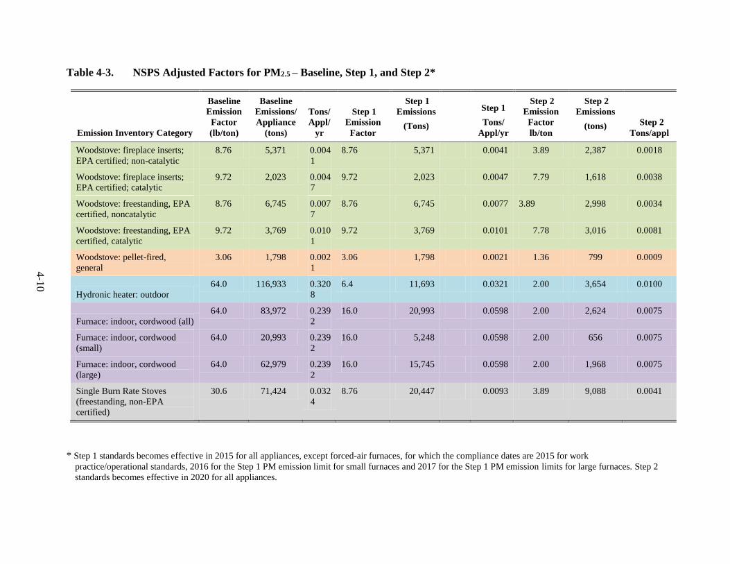
4-1
0
Table 4-3. NSPS Adjusted Factors for PM2.5 – Baseline, Step 1, and Step 2*
Emission Inventory Category
Baseline
Emission
Factor
(lb/ton)
Baseline
Emissions/
Appliance
(tons)
Tons/
Appl/
yr
Step 1
Emission
Factor
Step 1
Emissions
(Tons)
Step 1
Tons/
Appl/yr
Step 2
Emission
Factor
lb/ton
Step 2
Emissions
(tons) Step 2
Tons/appl
Woodstove: fireplace inserts;
EPA certified; non-catalytic
8.76 5,371 0.004
1
8.76 5,371 0.0041 3.89 2,387 0.0018
Woodstove: fireplace inserts;
EPA certified; catalytic
9.72 2,023 0.004
7
9.72 2,023 0.0047 7.79 1,618 0.0038
Woodstove: freestanding, EPA
certified, noncatalytic
8.76 6,745 0.007
7
8.76 6,745 0.0077 3.89 2,998 0.0034
Woodstove: freestanding, EPA
certified, catalytic
9.72 3,769 0.010
1
9.72 3,769 0.0101 7.78 3,016 0.0081
Woodstove: pellet-fired,
general
3.06 1,798 0.002
1
3.06 1,798 0.0021 1.36 799 0.0009
Hydronic heater: outdoor
64.0 116,933 0.320
8
6.4 11,693 0.0321 2.00 3,654 0.0100
Furnace: indoor, cordwood (all)
64.0 83,972 0.239
2
16.0 20,993 0.0598 2.00 2,624 0.0075
Furnace: indoor, cordwood
(small)
64.0 20,993 0.239
2
16.0 5,248 0.0598 2.00 656 0.0075
Furnace: indoor, cordwood
(large)
64.0 62,979 0.239
2
16.0 15,745 0.0598 2.00 1,968 0.0075
Single Burn Rate Stoves
(freestanding, non-EPA
certified)
30.6 71,424 0.032
4
8.76 20,447 0.0093 3.89 9,088 0.0041
* Step 1 standards becomes effective in 2015 for all appliances, except forced-air furnaces, for which the compliance dates are 2015 for work
practice/operational standards, 2016 for the Step 1 PM emission limit for small furnaces and 2017 for the Step 1 PM emission limits for large furnaces. Step 2
standards becomes effective in 2020 for all appliances.

4-1
1
4.2.2 Voluntary Programs
Within these emissions projections are the effects not only of rules but also of various
voluntary programs managed by EPA and states. Studies have shown that fine particle (PM2.5)
concentrations in proximity to a typical outdoor wood boiler are likely to exceed the 24-hour
National Ambient Air Quality Standards (NAAQS).18 Thus, the EPA developed the voluntary
Hydronic Heater Program to encourage manufacturers to reduce impacts on air quality through
developing and distributing cleaner, more efficient hydronic heaters. We developed the voluntary
program because it could bring cleaner models to market faster than the traditional federal
regulatory process. Phase 119 emission level (0.60 pounds per million British Thermal Unit
(lb/MMBTU) heat input) qualifying20 units are approximately 70% cleaner than typical
unqualified units. After March 31, 2010, units that only meet the Phase 1 emission level are no
longer considered “qualified models” under the voluntary program. Phase 2 emission level (0.32
lb/MMBTU heat output) qualifying units are approximately 90% cleaner than typical unqualified
units. Typically, qualified models have improved insulation, secondary combustion, separation
of the firebox from the water jacket, and the addition of improved heat exchangers.
In addition to the voluntary program, the EPA provided technical and financial support
for the Northeast States for Coordinated Air Use Management (NESCAUM) to develop a model
rule which several states have adopted to regulate residential wood hydronic heaters. The model
rule is a starting point for local regulatory authorities to consider, and they may need to also
adopt additional actions due to site-specific concerns, e.g., local terrain, meteorology, proximity
of neighbors and other exposed individuals. Thus, some regulatory authorities have instituted
additional requirements, including bans on hydronic heaters in some areas.
The EPA also developed a similar voluntary partnership program for low-mass fireplaces
(engineered, pre-fabricated fireplaces) and site-built masonry fireplaces. The original partnership
agreements were dated February 19, 2009, and pertained to low-mass fireplaces. On July 4,
2009, the program was expanded to other fireplaces, e.g., masonry fireplaces. Under this
18 For more information on wood smoke health effects, See: “Smoke Gets in Your Lungs: Outdoor Wood Boilers in
New York State,” prepared by Judith Schrieber, Ph.D., et al., for the Office of the Attorney General of New
York. August 2005. See also: “Assessment of Outdoor Wood-fired Boilers,” prepared by NESCAUM, March
2006 (revised June 2006). 19 Phase 1” and “Phase 2” emission levels refer to levels established in EPA voluntary programs. The earlier use of
the term “Phase II” (with a Roman numeral) standard refers to standards established in the current subpart AAA
for residential wood heaters. 20 The terms “qualified” and “unqualified,” or other similar terms, refer to models that meet the voluntary program
performance levels. Later use of the terms “certified” and “uncertified,” or other similar terms, refers to models
that are deemed to be in compliance with the NSPS emission limits.

4-1
2
program, cleaner burning fireplaces are ones that qualify for the Phase 1 emissions level of 7.3 g
of particles emitted per kg of fuel burned (approximately 57% cleaner than unqualified models)
or the Phase 2 emissions level of 5.1 g/kg (approximately 70% cleaner than unqualified models).
So far, 11 models have qualified under this voluntary program at the Phase 2 level. Typically,
qualified models have improved insulation and added secondary combustion and/or a catalyst to
reduce emissions. Some manufacturers have added closed doors to reduce the excess air and thus
improve combustion. Some state and local agencies have needed to reduce emissions further and
thus some have no-burn days and some have adopted bans of new fireplaces in some areas in
order to attain the PM2.5 NAAQS.
4.2.3 Shipment Data Used to Estimate Baseline Emissions
We used data in the Frost & Sullivan Market (F&S) report21 on 2008 shipments by
product category, and F&S revenue forecasts which incorporated the weak economy in years
2009 and 2010, to calculate the reduced number of shipments in years 2009 and 2010. Forced air
furnaces were outside the scope of the F&S report. Instead, we used manufacturer estimates of
total industry sales in 200822 and applied the F&S market factors to estimate shipments through
2010. The F&S wood stove numbers included both certified and non-certified stoves, so we
estimated numbers of non-certified stove shipments out of the total reported wood stove
category. 23 These shipments were deleted from the total wood stove category shipments. We
expanded the 2008 single burn rate estimate using the F&S factors. Our estimates of annual
shipments, truncated to 2020, are shown in Table 4-4. The full set of annual shipments data can
be found in the emissions memo for this final rule.
For years 2011 through 2029 (for the NSPS) estimated shipments are based on a
forecasted revenue growth rate of 2.0%, in keeping with the average annual growth in real U.S.
GDP predicted by the Conference Board.24 We use the average annual growth rate forecast from
the Conference Board as a basis for estimating future growth in shipments when specific
projections are not available. We do this since there are manufacturing industries in multiple
NAICS that are impacted by this final rule as noted in Section 3 of this RIA, and the economic
activity in these industries is typically reflective of changes in real GDP in the U.S. There is not
a perfect correlation between shipments and revenue (for example, because of their higher unit
21 Market Research and Report on North American Residential Wood Heaters, Fireplaces, and Hearth Heating
Products Market. Prepared by Frost & Sullivan. April 26, 2010. pp. 31-32. 22 NSPS Review and Comments. Confidential Business Information submitted by manufacturer. September 2010. 23 Memo to Gil Wood, USEPA, from EC/R, Inc. Estimated Emissions from Wood Heaters. January 30, 2015. 24 2014 Global Outlook projections prepared by the Conference Board in November 2013; http://www.conference-
board.org/data/globaloutlook.cfm

4-1
3
cost, pellet stoves generate more absolute revenue than wood stoves), but as stated in our
emissions memorandum, we think the overall trend in the projection is reasonable in the absence
of specific shipment projections. The only exceptions to the use of a 2.0% GDP-based growth
rate are for years 2012 and 2018, in which we used industry estimates for hydronic heater and
wood stove shipments, respectively. In addition, for year 2012, an HPBA consultant estimated
there were 13,100 baseline hydronic heater sales.26 For year 2018, the same HPBA consultant
projected there to be 100,000 wood stove sales.27 We adjusted our estimated shipment data
accordingly. The shipment data in Table 4-4 below includes presentation by indoor cordwood
furnace (forced air furnace) size categories as well for that entire appliance category.28
Table 4-4. Estimated Annual Shipments by Category, 2008-2020
2008 2009 2010 2011 2012 2013 2014 2015 2016 2017 2018 2019 2020
Wood
stoves
126,527 80,851 77,617 79,169 80,752 82,367 84,015 85,695 87,409 89,157 100,000 102,000 104,040
Single
burn rate
stoves
40,000 25,560 24,538 25,028 25,529 26,039 26,560 27,091 27,633 28,186 28,750 29,325 29,911
Pellet
stoves
130,381 83,313 79,981 81,581 83,212 84,876 86,574 88,305 90,072 91,873 93,710 95,585 97,496
Furnace:
indoor,
cordwood
(all)
41,000 26,199 25,151 25,654 26,167 26,690 27,224 27,769 28,324 28,891 29,468 30,058 30,659
Furnace:
indoor,
cordwood
(small)
10,250 6,550 6,288 6,414 6,542 6,673 6,806 6,942 7,081 7,223 7,367 7,514 7,665
Furnace:
indoor,
cordwood
(large)
30,250 19,649 18,863 19,241 19,625 20,018 20,418 20,827 21,243 21,668 22,101 22,543 22,994
Hydronic
heating
systems
13,385 8,553 8,211 8,375 13,100 13362 13,629 13,902 14,180 14,463 14,753 15,048 15,349
26 Cost-Effectiveness Analysis of Alternative Hydronic Heater New Source Performance Standards, prepared for the
Hearth, Patio, and Barbecue Association by NERA Economic Consulting, May 2014. 27 Cost-Effectiveness Analysis of Alternative Woodstove New Source Performance Standards, prepared for the
Hearth, Patio, and Barbecue Association by NERA Economic Consulting, May 2014. 28 Memorandum to Docket ID Number EPA-HQ-2009-0734 from EC/R, Inc. to U.S. EPA. Baseline and NSPS
emissions from small and large forced-air furnaces. February 2015.

4-1
4
Our cost effectiveness analysis (CE)29 assumes a 10-year model design lifespan as well as
a 20-year use/emitting appliance lifespan. These assumptions were made to best characterize the
actual model design and use lifespans. For proposal, we used a 20-year model design lifespan,
reasoning that many models developed for the 1988 NSPS are still being sold (after 25 years),
with many “new” models retaining the same internal working parts with merely exterior
cosmetic changes. Respectful of comments on the proposed rule30, however, in which some
industry representatives commented that a shorter model lifespan is more accurate, we reduced
our assumed model design lifespan to 10 years for this analysis. Regarding the emitting lifespan
of the appliance, most wood heaters in consumer homes emit for at least 20 years and often much
longer. Therefore our CE analysis tracks shipments through year 2029 (assuming a 10-year
design life for a model meeting the Step 2 limit in year 2020) and emissions through year 2048
(assuming a 20-year emitting life for an appliance shipped in year 2029). Table 4-4 is a truncated
summary of our actual shipment data which extended through years 2029. See the CE analysis
spreadsheets31 for the complete shipment data.
4.3 Estimated PM2.5 Emissions from Shipments of New Appliances
As described above, we calculated the average emissions per appliance type using the
emission factor for each category multiplied by the inventory value of total tons of wood burned
divided by the number of appliances in the inventory population. This value was then multiplied
by the number of shipments to calculate total emissions from each category per year under
baseline conditions (i.e., in the absence of an NSPS). Furthermore, in order not to overstate
emission reductions caused by the NSPS, baseline emissions were discounted by the percentage
of appliances already meeting the Step 2 PM emission limit (i.e., 26% of wood stoves, 70% of
pellet stoves, and 18% of hydronic heaters are estimated to already meet the Step 2 PM emission
limit). More information on these calculations is available in the emissions memorandum in the
docket for this rulemaking.26
Table 4-5 on the next page shows a truncated summary of the estimated PM2.5 emissions
(in tons) under baseline conditions through year 2020. We then estimated emissions under the
29 Memorandum to USEPA from EC/R, Inc. Residential Wood Heater Cost Effectiveness Analysis. January 30,
2015. 30 Comments on the proposed NSPS are available electronically through http://www.regulations.gov by searching
Docket IDs EPA-HQ-OAR-2009-0734. 31 See January 2015 cost effectiveness (CE) spreadsheets including for PM2.5 the Revised Final Wood Heater NSPS
PM CE 7% for the CE analysis supporting the NSPS. All of these spreadsheets are found in the public docket for
this rulemaking. 26 Memo to Gil Wood, USEPA, from EC/R, Inc. Estimated Emissions from Wood Heaters. January 30, 2015.
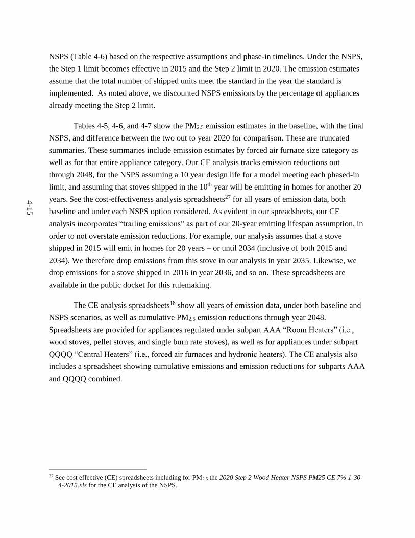
4-1
5
NSPS (Table 4-6) based on the respective assumptions and phase-in timelines. Under the NSPS,
the Step 1 limit becomes effective in 2015 and the Step 2 limit in 2020. The emission estimates
assume that the total number of shipped units meet the standard in the year the standard is
implemented. As noted above, we discounted NSPS emissions by the percentage of appliances
already meeting the Step 2 limit.
Tables 4-5, 4-6, and 4-7 show the PM2.5 emission estimates in the baseline, with the final
NSPS, and difference between the two out to year 2020 for comparison. These are truncated
summaries. These summaries include emission estimates by forced air furnace size category as
well as for that entire appliance category. Our CE analysis tracks emission reductions out
through 2048, for the NSPS assuming a 10 year design life for a model meeting each phased-in
limit, and assuming that stoves shipped in the 10th year will be emitting in homes for another 20
years. See the cost-effectiveness analysis spreadsheets27 for all years of emission data, both
baseline and under each NSPS option considered. As evident in our spreadsheets, our CE
analysis incorporates “trailing emissions” as part of our 20-year emitting lifespan assumption, in
order to not overstate emission reductions. For example, our analysis assumes that a stove
shipped in 2015 will emit in homes for 20 years – or until 2034 (inclusive of both 2015 and
2034). We therefore drop emissions from this stove in our analysis in year 2035. Likewise, we
drop emissions for a stove shipped in 2016 in year 2036, and so on. These spreadsheets are
available in the public docket for this rulemaking.
The CE analysis spreadsheets18 show all years of emission data, under both baseline and
NSPS scenarios, as well as cumulative PM2.5 emission reductions through year 2048.
Spreadsheets are provided for appliances regulated under subpart AAA “Room Heaters” (i.e.,
wood stoves, pellet stoves, and single burn rate stoves), as well as for appliances under subpart
QQQQ “Central Heaters” (i.e., forced air furnaces and hydronic heaters). The CE analysis also
includes a spreadsheet showing cumulative emissions and emission reductions for subparts AAA
and QQQQ combined.
27 See cost effective (CE) spreadsheets including for PM2.5 the 2020 Step 2 Wood Heater NSPS PM25 CE 7% 1-30-
4-2015.xls for the CE analysis of the NSPS.

4-16

4-1
7
Table 4-5. Estimated PM2.5 Emissions (Tons): Baseline*
2008 2009 2010 2011 2012 2013 2014 2015 2016 2017 2018 2019 2020
Wood stoves 563 360 345 352 359 367 374 381 389 397 445 454 463
Single burn rate
stoves
1,295 827 794 810 826 843 860 877 895 912 931 949 968
Pellet stoves 83 53 51 52 53 54 55 56 57 59 60 61 62
Furnace: indoor,
cordwood (all)
9,808 6,267 6,017 6,137 6,260 6,385 6,513 6,643 6,776 6,911 7,049 7,190 7,334
Furnace: indoor,
cordwood (small)
2,452 1,567 1,504 1,534 1,565 1,596 1,628 1,661 1,694 1,728 1,762 1,798 1,834
Furnace: indoor,
cordwood (large)
7,356 4,700 4,512 4,603 4,695 4,789 4,884 4,982 5,082 5,183 5,287 5,393 5,501
Hydronic heating
systems
3,520 2,250 2,160 2,203 3,446 3,514 3,585 3,656 3,730 3,804 3,880 3,958 4,037
Total 15,269 9.757 9,367 9,554 10,944 11,163 11,386 11,614 11,846 12,083 12,365 12,612 12,865
*Estimates are reduced for the percentage of appliances assumed to already meet the Step 2 PM emission limit (26% of wood stoves,
70% of pellet stoves and 18% of hydronic heaters), in order to not overstate emission reductions attributable to this NSPS.
Table 4-6. Estimated PM2.5 Emissions (Tons): NSPS**
2008 2009 2010 2011 2012 2013 2014 2015 2016 2017 2018 2019 2020
Wood stoves 563 360 345 352 359 367 374 381 389 397 445 454 259
Single burn rate
stoves
1,295 827 794 810 826 843 860 251 256 261 266 272 123
Pellet stoves 83 53 51 52 53 54 55 56 57 59 60 61 28
Furnace: indoor,
cordwood (all)
9,808 6,267 6,017 6,137 6,260 6,385 6,513 6,643 5,505 1,728 1,762 1,798 229

4-1
8
Furnace: indoor,
cordwood (small)
2,452 1,567 1,504 1,534 1,565 1,596 1,628 1,661 423 432 441 449 57
Furnace: indoor,
cordwood (large)
7,356 4,700 4,512 4,603 4.695 4,789 4,884 4,982 5,082 1,296 1,322 1,348 172
Hydronic heating
systems
3,520 2,250 2,160 2,203 3,446 3,514 3,585 366 373 380 388 396 126
Total 15,269 9,757 9,367 9,554 10,944 11,163 11,386 7,697 6,581 2,825 2,922 2,980 765
**Step 1 PM emission limit in 2015 and Step 2 PM emission limit in 2020 for all appliances, except forced-air furnaces have work practice/operational
standards in 2015, Step 1 PM emission limits for small furnaces in 2016, Step 1 PM emission limits for large furnaces in 2017 and Step 2 PM emission
limits for all furnaces in 2020. In order to not overstate emission reductions attributable to this NSPS, estimates are reduced for the percentage of
appliances estimated to already meet the Step 2 PM emission limits (26% of wood stoves, 70% of pellet stoves and 18% of hydronic heaters). In this
analysis, emission reductions for forced-air furnaces are not quantified for the work practice/operational standard required in 2015, although
stakeholders agree that work practice/operational standards will reduce emissions.
4-1
9
Table 4-7. Estimated PM2.5 Emission Reductions from the NSPS (Tons):
2008 2009 2010 2011 2012 2013 2014 2015 2016 2017 2018 2019 2020
Wood stoves 0 0 0 0 0 0 0 0 0 0 0 0 204
Single burn rate
stoves
0 0 0 0 0 0 0 626 639 651 665 677 845
Pellet stoves 0 0 0 0 0 0 0 0 0 0 0 0 34
Furnace:
indoor,
cordwood (all)
0 0 0 0 0 0 0 0 1,271 5,183 5,287 5,392 7,105
Furnace:
indoor,
cordwood
(small)
0 0 0 0 0 0 0 0 1,271 1,296 1,321 1,349 1,777
Furnace:
indoor,
cordwood
(large)
0 0 0 0 0 0 0 0 0 3,887 3,965 4,043 5,328
Hydronic
heating systems
0 0 0 0 0 0 0 3,290 3,357 3,424 3,492 3,562 3,911
Total 0 0 0 0 0 0 0 3,917 5,265 9,258 9,443 9,632 12,099
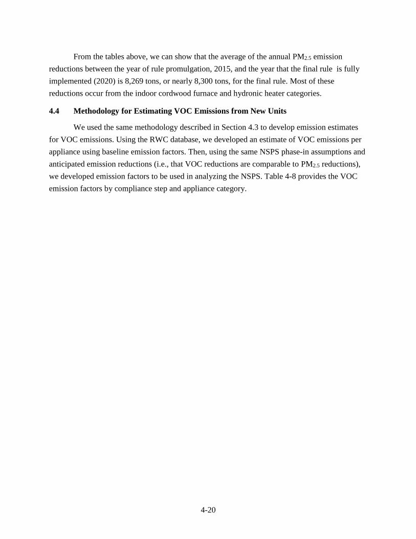
4-20
From the tables above, we can show that the average of the annual PM2.5 emission
reductions between the year of rule promulgation, 2015, and the year that the final rule is fully
implemented (2020) is 8,269 tons, or nearly 8,300 tons, for the final rule. Most of these
reductions occur from the indoor cordwood furnace and hydronic heater categories.
4.4 Methodology for Estimating VOC Emissions from New Units
We used the same methodology described in Section 4.3 to develop emission estimates
for VOC emissions. Using the RWC database, we developed an estimate of VOC emissions per
appliance using baseline emission factors. Then, using the same NSPS phase-in assumptions and
anticipated emission reductions (i.e., that VOC reductions are comparable to PM2.5 reductions),
we developed emission factors to be used in analyzing the NSPS. Table 4-8 provides the VOC
emission factors by compliance step and appliance category.
4-2
1
Table 4-8. NSPS VOC Emission Factors – Baseline, Step 1, and Step 2*
Emission Inventory Category
Baseline
Emission
Factor
(lb/ton)
Emissions
(tons)
Tons/
Appl/Yr
Step 1
Emission
Factor
(lb/ton)
Step 1
Emissions
(tons)
Step 1
Tons/
Appl/Yr
Step 2
Emission
Factor
(lb/ton)
Step 2
Emissions
(tons)
Alt. Step 2
Tons/
Appl/Yr
Woodstove: fireplace inserts;
EPA certified; non-catalytic
12.00 7,357 0.0056 12.00 7,357 0.0056 5.33 3,270 0.0025
Woodstove: fireplace inserts;
EPA certified; catalytic
15.00 3,121 0.0073 15.00 3,121 0.0073 12.00 2,497 0.0058
Woodstove: freestanding, EPA
certified, non-catalytic
12.00 9,240 0.0106 12.00 9,240 0.0106 5.33 4,107 0.0047
Woodstove: freestanding, EPA
certified, catalytic
15.00 5,817 0.0155 15.00 5,817 0.0155 12.00 4,654 0.0124
Woodstove: pellet-fired, general 0.041 24 0.0000 0.041 24 0.0000 0.02 11 0.0000
Hydronic heater: outdoor 67.4 123,145 0.3378 6.74 12,314 0.0338 2.11 3,848 0.0106
Furnace: indoor, cordwood (all) 67.4 88,433 0.2519 16.85 22,108 0.0630 2.11 2,764 0.0079
Furnace: indoor, cordwood
(small)
67.4 22,108 0.2519 16.85 5,527 0.0630 2.11 691 0.0079
Furnace: indoor, cordwood (large) 67.4 66,325 0.2519 16.85 16,581 0.0630 2.11 2,073 0.0079
Single burn rate stoves
(freestanding, non-EPA certified)
53.00 123,709 0.0561 12.00 28,010 0.0127 5.33 12,449 0.0056
* Step 1 PM standard becomes effective in 2015 for all appliances, except forced-air furnaces, for which the compliance dates are 2015 for work
practice/operational standards, 2016 for the Step 1 PM emission limit for small furnaces and 2017 for the Step 1 PM emission limit for large furnaces. Step 2
standards become effective in 2020 for all appliances.
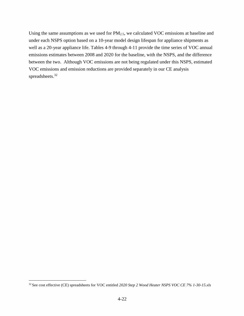
4-22
Using the same assumptions as we used for PM2.5, we calculated VOC emissions at baseline and
under each NSPS option based on a 10-year model design lifespan for appliance shipments as
well as a 20-year appliance life. Tables 4-9 through 4-11 provide the time series of VOC annual
emissions estimates between 2008 and 2020 for the baseline, with the NSPS, and the difference
between the two. Although VOC emissions are not being regulated under this NSPS, estimated
VOC emissions and emission reductions are provided separately in our CE analysis
spreadsheets.32
32 See cost effective (CE) spreadsheets for VOC entitled 2020 Step 2 Wood Heater NSPS VOC CE 7% 1-30-15.xls
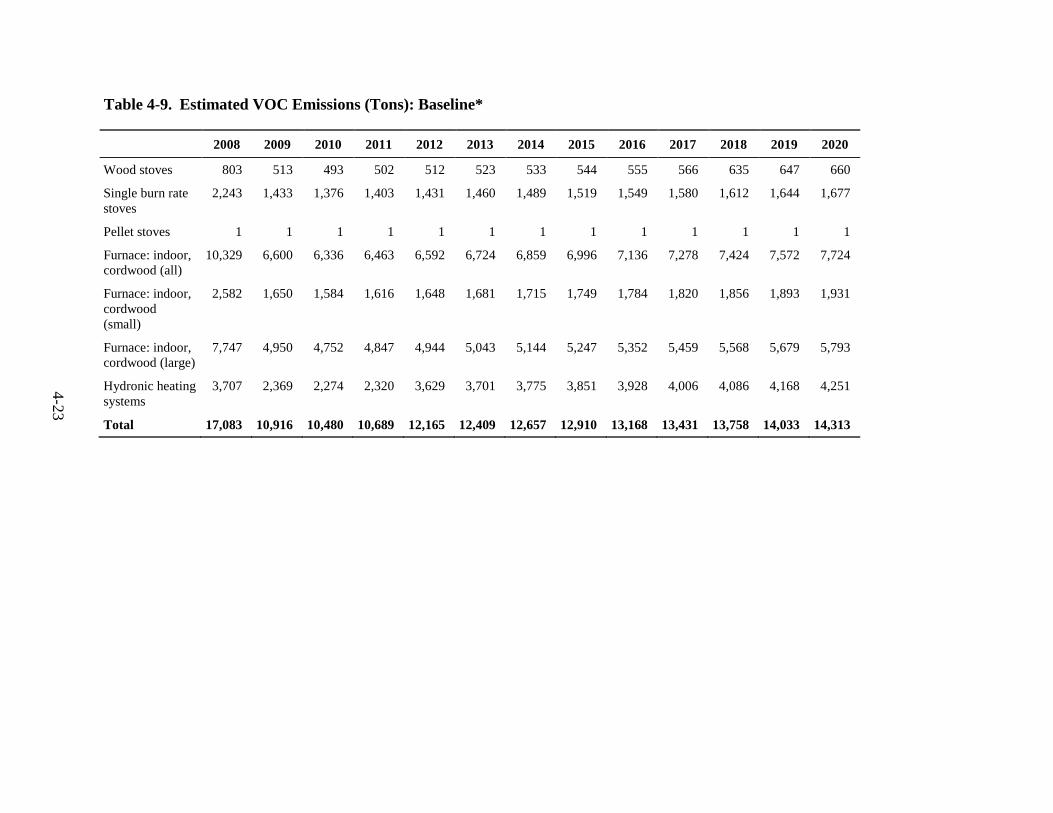
4-2
3
Table 4-9. Estimated VOC Emissions (Tons): Baseline*
2008 2009 2010 2011 2012 2013 2014 2015 2016 2017 2018 2019 2020
Wood stoves 803 513 493 502 512 523 533 544 555 566 635 647 660
Single burn rate
stoves
2,243 1,433 1,376 1,403 1,431 1,460 1,489 1,519 1,549 1,580 1,612 1,644 1,677
Pellet stoves 1 1 1 1 1 1 1 1 1 1 1 1 1
Furnace: indoor,
cordwood (all)
10,329 6,600 6,336 6,463 6,592 6,724 6,859 6,996 7,136 7,278 7,424 7,572 7,724
Furnace: indoor,
cordwood
(small)
2,582 1,650 1,584 1,616 1,648 1,681 1,715 1,749 1,784 1,820 1,856 1,893 1,931
Furnace: indoor,
cordwood (large)
7,747 4,950 4,752 4,847 4,944 5,043 5,144 5,247 5,352 5,459 5,568 5,679 5,793
Hydronic heating
systems
3,707 2,369 2,274 2,320 3,629 3,701 3,775 3,851 3,928 4,006 4,086 4,168 4,251
Total 17,083 10,916 10,480 10,689 12,165 12,409 12,657 12,910 13,168 13,431 13,758 14,033 14,313

4-2
4
Table 4-10. Estimated VOC Emissions (Tons): NSPS*
2008 2009 2010 2011 2012 2013 2014 2015 2016 2017 2018 2019 2020
Wood stoves 803 513 493 502 512 523 533 544 555 566 635 647 376
Single burn rate
stoves
2,243 1,433 1,376 1,403 1,431 1,460 1,489 344 351 358 365 372 169
Pellet stoves 1 1 1 1 1 1 1 1 1 1 1 1 0
Furnace: indoor,
cordwood (all)
10,329 6,600 6,336 6,463 6,592 6,724 6,859 6,996 5,798 1,820 1,856 1,893 241
Furnace: indoor,
cordwood
(small)
2,582 1,650 1,584 1,616 1,648 1,681 1,715 1,749 446 455 464 473 60
Furnace: indoor,
cordwood (large)
7,747 4,950 4,752 4,847 4,944 5,043 5,144 5,247 5,352 1,365 1,392 1,420 181
Hydronic heating
systems
3,707 2,369 2,274 2,320 3,629 3,701 3,775 385 393 401 409 417 133
Total 17,083 10,916 10,480 10,689 12,165 12,409 12,657 8,269 7,097 3,145 3,265 3,330 919
* Step 1 PM emission limit in 2015 and Step 2 PM emission limit in 2020 for all appliances, except forced-air furnaces have work practice/operational standards
in 2015, Step 1 PM emission limits for small furnaces in 2016, Step 1 PM emission limits for large furnaces in 2017 and Step 2 PM emission limits for all
furnaces in 2020. In order to not overstate emission reductions attributable to this NSPS, estimates are reduced for the percentage of appliances estimated to
already meet the Step 2 PM emission limits (26% of wood stoves, 70% of pellet stoves and 18% of hydronic heaters). In this analysis, emission reductions for
forced-air furnaces are not quantified for the work practice/operational standard required in 2015, although stakeholders agree that work practice/operational
standards will reduce emissions.

4-2
5
Table 4-11. Estimated VOC Emission Reductions from the NSPS (Tons):
2008 2009 2010 2011 2012 2013 2014 2015 2016 2017 2018 2019 2020
Wood stoves 0 0 0 0 0 0 0 0 0 0 0 0 284
Single burn rate
stoves
0 0 0 0 0 0 0 1,175 1,198 1,222 1,247 1,272 1,508
Pellet stoves 0 0 0 0 0 0 0 0 0 0 0 0 0
Furnace: indoor,
cordwood (all)
0 0 0 0 0 0 0 0 1,338 5,458 5,568 5,679 7,483
Furnace: indoor,
cordwood
(small)
0 0 0 0 0 0 0 0 1,338 1,365 1,392 1,420 1,871
Furnace: indoor,
cordwood (large)
0 0 0 0 0 0 0 0 0 4,094 4,176 4,259 5,612
Hydronic heating
systems
0 0 0 0 0 0 0 3,466 3,535 3,606 3,678 3,751 4,119
Total 0 0 0 0 0 0 0 4,641 6,071 10,287 10,493 10,702 13,394

4-26
From the tables above, we can show that the average of the annual emission reductions
between the year of rule promulgation, 2015, and the year that the NSPS is fully implemented
(2020) is 9,265 tons, or nearly 9,300 tons, for the final rule.
4.5 Methodology for Estimating CO Emissions from New Units
We used the same methodology described in Section 4.3 to develop estimates for CO
emissions. Using the RWC database, we developed an estimate of CO emissions per appliance
using baseline emission factors. Then, using the same NSPS phase-in assumptions and
anticipated emission reductions (i.e., that CO reductions are comparable to PM2.5 reductions), we
developed emission factors to be used in analyzing the changes in emissions from applying the
NSPS. Table 4-12 presents the CO emission factors by compliance step and appliance category.
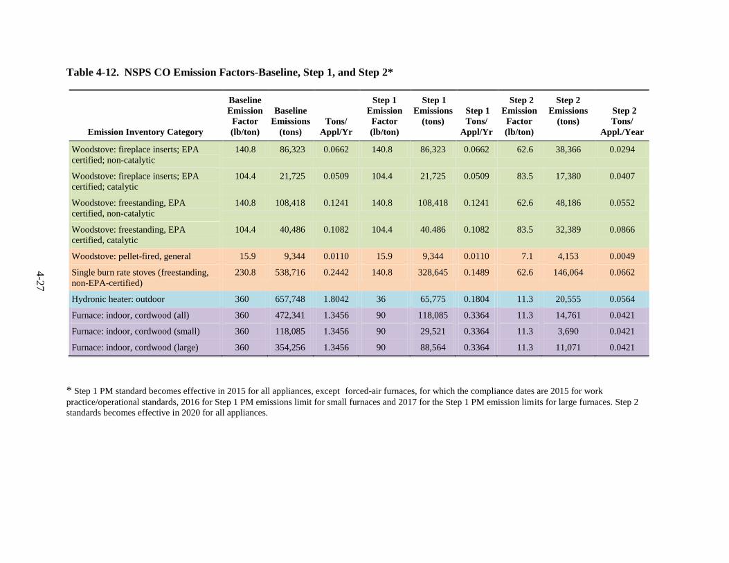
4-2
7
Table 4-12. NSPS CO Emission Factors-Baseline, Step 1, and Step 2*
Emission Inventory Category
Baseline
Emission
Factor
(lb/ton)
Baseline
Emissions
(tons)
Tons/
Appl/Yr
Step 1
Emission
Factor
(lb/ton)
Step 1
Emissions
(tons)
Step 1
Tons/
Appl/Yr
Step 2
Emission
Factor
(lb/ton)
Step 2
Emissions
(tons)
Step 2
Tons/
Appl./Year
Woodstove: fireplace inserts; EPA
certified; non-catalytic
140.8 86,323 0.0662 140.8 86,323 0.0662 62.6 38,366 0.0294
Woodstove: fireplace inserts; EPA
certified; catalytic
104.4 21,725 0.0509 104.4 21,725 0.0509 83.5 17,380 0.0407
Woodstove: freestanding, EPA
certified, non-catalytic
140.8 108,418 0.1241 140.8 108,418 0.1241 62.6 48,186 0.0552
Woodstove: freestanding, EPA
certified, catalytic
104.4 40,486 0.1082 104.4 40.486 0.1082 83.5 32,389 0.0866
Woodstove: pellet-fired, general 15.9 9,344 0.0110 15.9 9,344 0.0110 7.1 4,153 0.0049
Single burn rate stoves (freestanding,
non-EPA-certified)
230.8 538,716 0.2442 140.8 328,645 0.1489 62.6 146,064 0.0662
Hydronic heater: outdoor 360 657,748 1.8042 36 65,775 0.1804 11.3 20,555 0.0564
Furnace: indoor, cordwood (all) 360 472,341 1.3456 90 118,085 0.3364 11.3 14,761 0.0421
Furnace: indoor, cordwood (small) 360 118,085 1.3456 90 29,521 0.3364 11.3 3,690 0.0421
Furnace: indoor, cordwood (large) 360 354,256 1.3456 90 88,564 0.3364 11.3 11,071 0.0421
* Step 1 PM standard becomes effective in 2015 for all appliances, except forced-air furnaces, for which the compliance dates are 2015 for work
practice/operational standards, 2016 for Step 1 PM emissions limit for small furnaces and 2017 for the Step 1 PM emission limits for large furnaces. Step 2
standards becomes effective in 2020 for all appliances.

4-28
Using the same assumptions as we used for PM2.5, we calculated CO emissions at
baseline and for the NSPS. Table 4-13 shows the annual baseline emissions for CO for 2008 to
2020, and Tables 4-14 and 4-15 show the CO emissions with the NSPS and difference between
the two. Although CO emissions are not being regulated under this NSPS, estimated CO
emissions and emission reductions are provided separately in our CE analysis spreadsheets.33
33 See cost effective (CE) spreadsheets for CO entitled 2020 Step 2 Wood Heater NSPS CO CE 7%1-30-15.xls.
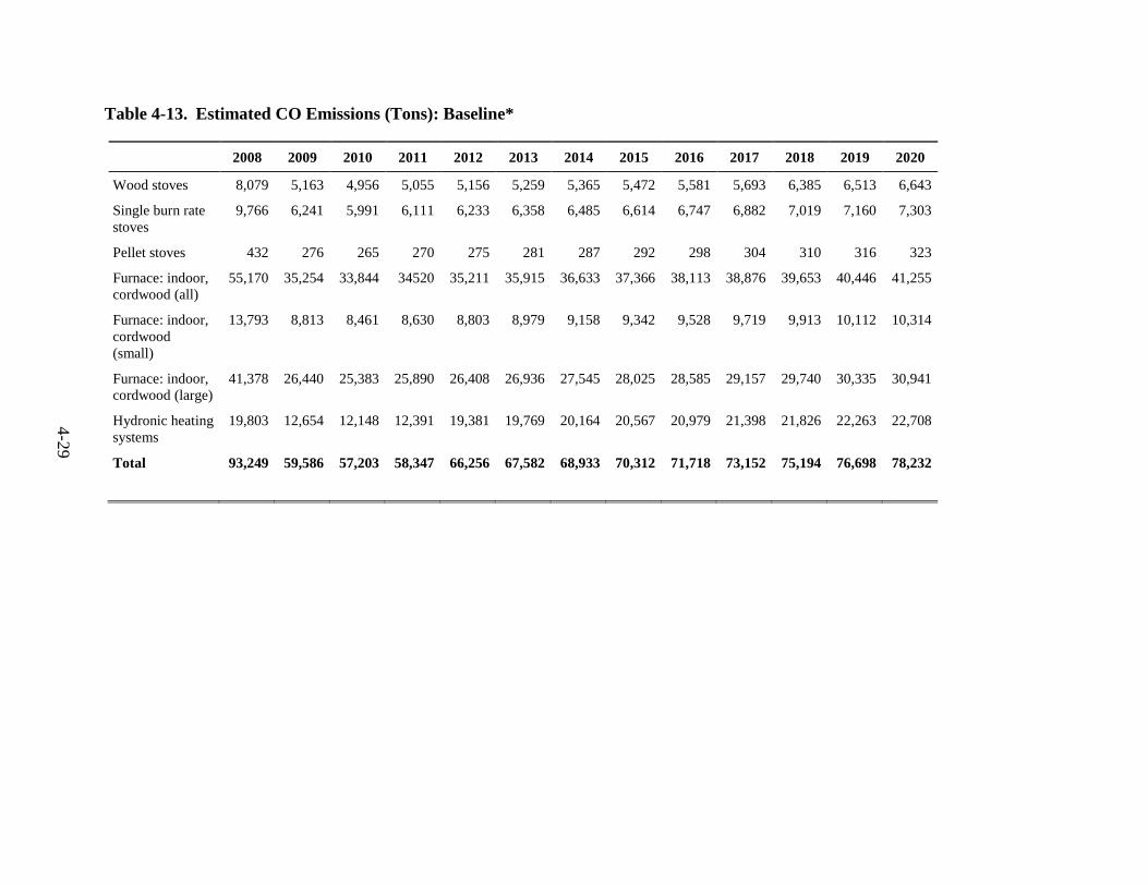
4-2
9
Table 4-13. Estimated CO Emissions (Tons): Baseline*
2008 2009 2010 2011 2012 2013 2014 2015 2016 2017 2018 2019 2020
Wood stoves 8,079 5,163 4,956 5,055 5,156 5,259 5,365 5,472 5,581 5,693 6,385 6,513 6,643
Single burn rate
stoves
9,766 6,241 5,991 6,111 6,233 6,358 6,485 6,614 6,747 6,882 7,019 7,160 7,303
Pellet stoves 432 276 265 270 275 281 287 292 298 304 310 316 323
Furnace: indoor,
cordwood (all)
55,170 35,254 33,844 34520 35,211 35,915 36,633 37,366 38,113 38,876 39,653 40,446 41,255
Furnace: indoor,
cordwood
(small)
13,793 8,813 8,461 8,630 8,803 8,979 9,158 9,342 9,528 9,719 9,913 10,112 10,314
Furnace: indoor,
cordwood (large)
41,378 26,440 25,383 25,890 26,408 26,936 27,545 28,025 28,585 29,157 29,740 30,335 30,941
Hydronic heating
systems
19,803 12,654 12,148 12,391 19,381 19,769 20,164 20,567 20,979 21,398 21,826 22,263 22,708
Total 93,249 59,586 57,203 58,347 66,256 67,582 68,933 70,312 71,718 73,152 75,194 76,698 78,232

4-3
0
Table 4-14. Estimated CO Emissions (Tons): NSPS*
2008 2009 2010 2011 2012 2013 2014 2015 2016 2017 2018 2019 2020
Wood stoves 8,079 5,163 4,956 5,055 5,156 5,259 5,365 5,472 5,581 5,693 6,385 6,513 3,524
Single burn rate
stoves
9,766 6,241 5,991 6,111 6,233 6,358 6,485 4,035 4,116 4,198 4,282 4,368 1,980
Pellet stoves 432 276 265 270 275 281 287 292 298 304 310 316 143
Furnace: indoor,
cordwood (all)
55,170 35,254 33,844 34,520 35,211 35,915 36,633 37,366 2,383 9,719 9,913 10,112 1,289
Furnace: indoor,
cordwood
(small)
13,793 8,813 8,461 8,630 8,803 8,979 9,158 9,342 2,382 2,430 2,478 2,528 322
Furnace: indoor,
cordwood (large)
41,378 26,440 25,383 25,890 26,408 26,936 27,475 28,025 28,585 7,289 7,435 7,584 967
Hydronic heating
systems
19,803 12,654 12,198 12,391 19,381 19,769 20,164 2,057 2,098 2,140 2,183, 2,226 710
Total 93,249 59,586 57,203 58,347 66,256 67,582 68,933 49,222 43,060 22,054 23,073 23,535 7,647
* Step 1 PM emission limit in 2015 and Step 2 PM emission limit in 2020 for all appliances, except forced-air furnaces have work practice/operational
standards in 2015, Step 1 PM emission limits for small furnaces in 2016, Step 1 PM emission limits for large furnaces in 2017 and Step 2 PM emission
limits for all furnaces in 2020. In order to not overstate emission reductions attributable to this NSPS, estimates are reduced for the percentage of
appliances estimated to already meet the Step 2 PM emission limits (26% of wood stoves, 70% of pellet stoves and 18% of hydronic heaters). In this
analysis, emission reductions for forced-air furnaces are not quantified for the work practice/operational standard required in 2015, although
stakeholders agree that work practice/operational standards will reduce emissions.
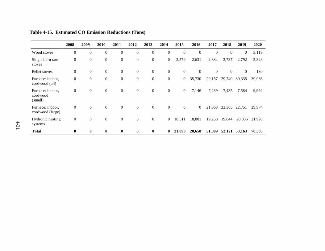
4-3
1
Table 4-15. Estimated CO Emission Reductions (Tons)
2008 2009 2010 2011 2012 2013 2014 2015 2016 2017 2018 2019 2020
Wood stoves 0 0 0 0 0 0 0 0 0 0 0 0 3,119
Single burn rate
stoves
0 0 0 0 0 0 0 2,579 2,631 2,684 2,737 2,792 5,323
Pellet stoves 0 0 0 0 0 0 0 0 0 0 0 0 180
Furnace: indoor,
cordwood (all)
0 0 0 0 0 0 0 0 35,730 29,157 29,740 30,335 39,966
Furnace: indoor,
cordwood
(small)
0 0 0 0 0 0 0 0 7,146 7,289 7,435 7,584 9,992
Furnace: indoor,
cordwood (large)
0 0 0 0 0 0 0 0 0 21,868 22,305 22,751 29,974
Hydronic heating
systems
0 0 0 0 0 0 0 18,511 18,881 19,258 19,644 20,036 21,998
Total 0 0 0 0 0 0 0 21,090 28,658 51,099 52,121 53,163 70,585

4-32
From the tables above, we can show that the average of the annual CO emission reductions
between the year of rule promulgation, 2015, and the year that the NSPS is fully implemented
(2020) is 46,119 tons, or just over 46,000 tons.
Sensitivity analyses of these emission estimates were prepared for GDP growth rates of
2.1%, 2.5%, and 3.0%. These analyses can be found in Appendix A of the cost-effectiveness
memorandum for the final rule.34
34 Memo to Gil Wood and David Cole, US EPA from EC/R, Inc. Residential Wood Heater Cost Effectiveness
Analysis. January 30, 2015. Appendix A.
5-1
SECTION 5
COST ANALYSIS, ENERGY IMPACTS, AND EXECUTIVE ORDER ANALYSES
In this section, we provide the estimates of total compliance costs and background behind
their estimation. The estimates of compliance costs use the control cost methodology employed
in the EPA Air Pollution Control Cost Manual to estimate capital and annual costs,46 and
incorporate some of the data provided by commenters on the proposal as explained in the
section. In addition, we provide a qualitative economic impact analysis of the proposed rule’s
impact on consumer and producer decisions, a qualitative discussion on unfunded mandates that
may occur as a result of this final rule, and a partial analysis of the impacts of this rule on
employment. We used the direct annual compliance costs as an approximate measure of total
social costs.
Given these constraints, several economic frameworks can be used to estimate the
economic impacts and social costs of regulations; however, OAQPS has traditionally relied on
partial equilibrium market models. Previous NSPS economic impact analyses for the residential
wood stove market were prepared reflecting such a model standpoint. However, the current data
do not provide sufficient details to develop a market model; the data that are available have little
or no sector/firm detail and are reported at the national level. In addition, some sectors have
unique market characteristics that make developing partial equilibrium models difficult.
Therefore, we have prepared the economic impact analysis including a qualitative partial
equilibrium framework.
The costs for the final rule are higher than those for the proposal rule. Changes to the
cost analyses from the proposal to the final rule are included in the presentation of the cost
analyses below.
5.1 Background for Compliance Costs
5.1.1 Estimated Research and Development (R&D) Costs
5.1.1.1 Model Development Costs – Room Heaters
Prior to proposal of the NSPS, EPA received various estimates of the costs to bring a
wood heater from concept to completion, from $200,000 for a single model to $1,360,000 for a
4-firebox model line. For example, a recent Hearth and Home article 47estimated the total cost to
46 EPA Air Pollution Control Cost Manual. 2002. Sixth Edition. Available on the Internet at
http://epa.gov/ttn/catc/products.html#cccinfo. 47 James E. Houck and Paul Tiegs. There’s a Freight Train Comin’. Hearth and Home. December 2009.
5-2
bring a model from conception to market as $645,000 to $750,000 for steel stoves and over $1
million for cast-iron, enameled wood stoves. The authors indicated that costs would decrease for
separate models in the same line by up to 25%. Based on this information, we estimate that a 4-
model steel line would cost up to $328,000 per model to develop. These costs include marketing,
design, developing first generation, second generation and prototype units; NSPS and safety
testing, equipment tooling, etc. The manufacturer supplying these figures for the article
estimated that the NSPS and safety testing component of these costs would constitute $40,000
per model. Two other manufacturers also provided estimated development costs for a 4-box
model line, and based on that information we estimated average costs to develop a new model
line, including testing with both crib and cord wood and reporting and recordkeeping, of
$356,000 for certified wood stoves and pellet stoves. We also assumed $356,000 for single burn
rate stoves, which may be somewhat high if they are as clean as the manufacturers claim. We
likewise assumed a development cost of $356,000 for forced air furnaces and hydronic heaters.
Comments received on the proposed rule included information and opinions regarding
these wood heater cost estimates.48 Comments ranged from criticism that the EPA overestimated
costs to criticism that the EPA underestimated costs. For example, one commenter stated that the
proposal cost estimates were overly generous and did not address input from Woodstock
Soapstone Stoves, winner of the 2013 Wood Stove Decathlon, which estimates that the cost of
new product development is approximately $200,000, and furthermore that the proposal cost
estimates did not address the economies manufacturers realize when they develop functionally
identical models from the originally certified model.49 Other commenters generally stated that
the breakdown of cost estimates faced by manufacturers is inaccurately low.
One commenter, in particular, provided detailed estimates of adjustable burn rate wood
stoves and hydronic heater model development costs. According to this commenter, the proposal
cost estimates are deficient because they do not reflect specific emission rates or emission
performances. The commenter provided cost estimates for categories not covered specifically in
EPA’s cost analysis for the proposal nor by the NSPS. The detailed wood stove cost estimates
are located in Attachment 2 of the Hearth, Patio and Barbeque Association (HPBA) comments
and were prepared by NERA Economic Consulting (May 2014).50 Appendix A of the document,
48 Comments on the proposed NSPS are available electronically through http://www.regulations.gov by searching
Docket ID EPA-HQ-OAR-2009-0734. 49 Comment on the proposed rule to Docket EPA-HQ-OAR-2009-0734 from the Washington State Department of
Ecology; available at http://www.regulations.gov/#!documentDetail;D=EPA-HQ-OAR-2009-0734-1397 50 Comment on the proposed rule to Docket EPA-HQ-OAR-2009-0734 from the Hearth, Patio and Barbeque
Association available at http://www.regulations.gov/#!documentDetail;D=EPA-HQ-OAR-2009-0734-1643
5-3
Woodstove Cost Modeling (prepared by Ferguson, Andors & Company) contains the detailed
cost estimates we reviewed and adapted for this analysis. According to Appendix A, “…a
‘bottom-up’ approach was used to identify the relevant components of compliance costs and to
develop a range of cost estimates for each cost component based on [their] extensive experience
in woodstove development, testing and manufacturing. The cost estimates were focused on mid-
sized non-catalytic stove models since those models currently represent the biggest segment of
the market. In developing the cost estimates, [they] incorporated detailed comments from a
review panel consisting of ten industry experts. The range of cost estimates resulting from this
process are representative of typical manufacturers and typical woodstove models, but actual
costs for particular manufacturers could lie outside the range. NERA used the mid-points
(averages) of the cost ranges for the cost-effectiveness analysis.”51
The Ferguson analysis provides cost estimates for four categories of emission reductions
based on the proposed emission levels, consisting of modifying 7.5 g/hr stoves to comply with a
new 4.5 g/hr standard, modifying the 4.5 g/hr stoves to comply with new standards of 2.5 g/hr or
1.3 g/hr stoves, and modifying a 2.5 g/hr stove to a new standard of 1.3 g/hr. The resulting cost
components consisted of capital costs per model (R&D, engineering labor, tooling, equipment
integration, preliminary testing, and other costs to design and manufacture the modified wood
stove model) and other fixed costs per model (certification testing and safety testing, roll-out of
the modified products including store display models and burn programs, brochures, user
manuals, training and product discounts). The mid-point capital costs presented by Ferguson
range from $281,725 to $532,050 depending on the emission reduction range.52
Unlike the proposed rule, the final rule only contains a Step 1 PM emission limit of 4.5
g/hr and a Step 2 PM emission limit of 2.0 g/hr, with no alternative, three-step limits. We
maintain that the Step 1 cost for 7.5 to 4.5 g/hr is a reasonable representation of model
development costs for all models subject to subpart AAA, with some exceptions, described
below. The Ferguson analysis shows that several of the cost components are identical across
scenarios. The analysis claims, however, that other cost components vary according to the
specified emission reduction scenario. We found these differences to be unsupported. For
51 Ferguson, Robert (Ferguson, Andors & Company), prepared for the Hearth, Patio & Barbecue Association.
Proposed Wood Heater NSPS Incremental Cost Effectiveness Analyses, Appendix A: Woodstove Cost
Modeling. May 2014. p. 1. 52 Ferguson, Robert (Ferguson, Andors & Company), prepared for the Hearth, Patio & Barbecue Association.
Proposed Wood Heater NSPS Incremental Cost Effectiveness Analyses, Appendix A: Woodstove Cost
Modeling. May 2014. pp. 4 – 5.
5-4
purposes of this analysis, we used the 7.5 to 4.5 g/hr scenario as a baseline case and modified it
to reflect the deletion of cost categories that we deemed inappropriately attributed to the NSPS.
We did accept the assumptions and logic related to evaluating the tooling cost differences
between steel stoves and cast iron stoves, as both are commonly manufactured. Like Ferguson,
we used an average of their tooling costs to reflect product differences, even though we believe
this may overestimate the number of cast iron stoves in the market place. While we recognize the
range in capital cost estimates provided both prior to and after proposal of the draft standards
leave room for additional cost scenarios, especially the much lower cost scenario for Woodstock
Soapstone Stoves, we concluded that the Ferguson costs represent the best documented cost
ranges and cost categories available at this time. Table 5-1, below, is a summary of the estimated
wood stove capital costs used in our analyses.
For the final cost analysis, we used the mean wood stove costs estimated in Table 5-1.
We have assumed that these model development costs represent feasible costs for adjustable
burn rate stoves and pellet stoves. For single burn rate stoves, we believe, as we did at proposal,
that additional R&D may be required to bring these stoves to qualifying levels. In addition,
testing with cordwood is not required for all of these appliances as mentioned in Section 2 of this
RIA and the preamble, so the costs presented here accordingly reflect that. Therefore, we
estimated that the R&D/Engineering cost portion of the total costs would require double the
investment in the first 2 years, with “normal” model development proceeding thereafter.
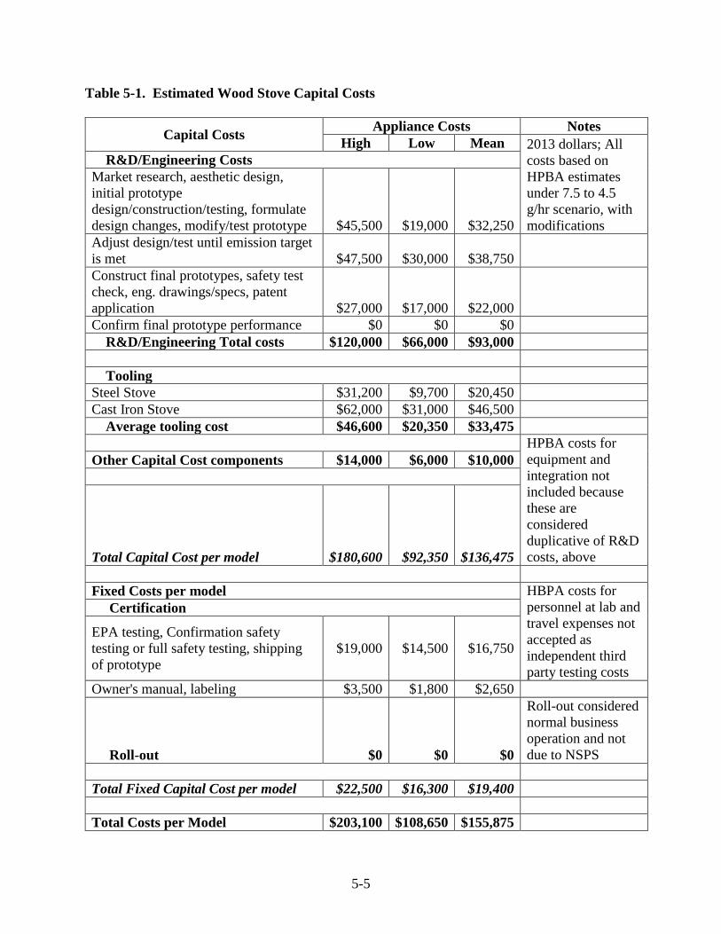
5-5
Table 5-1. Estimated Wood Stove Capital Costs
Capital Costs Appliance Costs Notes
High Low Mean 2013 dollars; All
costs based on
HPBA estimates
under 7.5 to 4.5
g/hr scenario, with
modifications
R&D/Engineering Costs
Market research, aesthetic design,
initial prototype
design/construction/testing, formulate
design changes, modify/test prototype $45,500 $19,000 $32,250
Adjust design/test until emission target
is met $47,500 $30,000 $38,750
Construct final prototypes, safety test
check, eng. drawings/specs, patent
application $27,000 $17,000 $22,000
Confirm final prototype performance $0 $0 $0
R&D/Engineering Total costs $120,000 $66,000 $93,000
Tooling
Steel Stove $31,200 $9,700 $20,450
Cast Iron Stove $62,000 $31,000 $46,500
Average tooling cost $46,600 $20,350 $33,475
HPBA costs for
equipment and
integration not
included because
these are
considered
duplicative of R&D
costs, above
Other Capital Cost components $14,000 $6,000 $10,000
Total Capital Cost per model $180,600 $92,350 $136,475
Fixed Costs per model HBPA costs for
personnel at lab and
travel expenses not
accepted as
independent third
party testing costs
Certification
EPA testing, Confirmation safety
testing or full safety testing, shipping
of prototype
$19,000 $14,500 $16,750
Owner's manual, labeling $3,500 $1,800 $2,650
Roll-out $0 $0 $0
Roll-out considered
normal business
operation and not
due to NSPS
Total Fixed Capital Cost per model $22,500 $16,300 $19,400
Total Costs per Model $203,100 $108,650 $155,875

5-6
Annualized capital cost per model $42,610 $22,794 $32,702 Annualized over 6
years at 7%
Annualized capital cost for
development of 4 models $170,438 $91,177 $130,808

5-7
5.1.2 Model Development Costs – Central Heaters
At proposal, we assumed that hydronic heaters and forced air furnaces would face the
same model development costs as room heaters. Some commenters objected to this
characterization, particularly based on the detailed hydronic heater cost estimates located in
Attachment 3 of the HPBA comments as prepared by NERA Economic Consulting (May
2014).53 Appendix A of that document, Hydronic Heater Cost Modeling (prepared by Ferguson,
Andors & Company) contains the detailed cost estimates we reviewed and adapted for this
analysis.
These costs were prepared with the same methodology and overall assumptions as were
used in development of the wood heater costs. The Ferguson analysis provides cost estimates for
four categories of hydronic heater emission reductions, based on the proposed emission levels
consisting of modifying uncontrolled heaters to comply with a new 0.32 lb/MMBtu standard,
modifying the 0.32 lb/MMBtu heaters to comply with new standards of 0.15 or 0.06 lb/MMBtu,
and modifying a 0.15 lb/MMBtu heater to a new standard of 0.06 lb/MMBtu. The resulting cost
components consisted of capital costs per model (R&D, engineering labor, tooling, equipment
integration, preliminary testing, and other costs to design and manufacture the modified wood
stove model) and other fixed costs per model (certification testing and safety testing, roll-out of
the modified products including store display models and burn programs, brochures, user
manuals, training and product discounts). The mid-point capital costs presented by Ferguson
range from $1,743,750 to $2,162,300 depending on the emission reduction range.54
Unlike the proposed rule, the final rule only contains a Step 1 PM emission limit of 0.32
lb/MMBtu and a Step 2 PM emission limit of 0.1 lb/MMBtu, with no alternative three-step
limits. We estimate that the Step 1 PM emission limit cost for uncontrolled to 0.32 lb/MMBtu is
a reasonable representation of model development costs for all models subject to subpart QQQQ,
with some exceptions, described below. The Ferguson analysis shows that several of the cost
components are identical across scenarios. The analysis claims, however, that other cost
components vary according to the specified emission reduction scenario. We found these
differences to be unsupported. For purposes of this analysis, we used the uncontrolled to 0.32
53 Comment on the proposed rule to Docket EPA-HQ-OAR-2009-0734 from the Hearth, Patio and Barbeque
Association available at http://www.regulations.gov/#!documentDetail;D=EPA-HQ-OAR-2009-0734-1643 54 Ferguson, Robert (Ferguson, Andors & Company), prepared for the Hearth, Patio & Barbecue Association.
Proposed Wood Heater NSPS Incremental Cost Effectiveness Analyses, Appendix A: Hydronic Heater Cost
Modeling. May 2014. p. 4.

5-8
lb/MMBtu as a baseline case and modified it to reflect the deletion of cost categories that we
deemed inappropriately attributed to the NSPS.
For the final cost analysis, we used the mean hydronic heater costs estimated in Table 5-
2 below. We have assumed that these model development costs represent feasible costs for
hydronic heaters. For forced air furnaces, we estimate, as we did at proposal, that additional
R&D may be required to bring these heaters to qualifying levels. Rather than doubling total
model development costs during the first 2 years as we did at proposal, we assumed that the
R&D/Engineering cost portion of the total costs would require double the investment in the first
2 years, with “normal” model development proceeding thereafter. This revised assumption is
consistent with information provided in public comments. In addition, testing with cordwood is
not required for these appliances as mentioned in Section 2 of this RIA and the preamble (though
the test method is based on cord wood), so the costs presented here accordingly reflect.
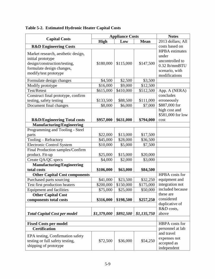
5-9
Table 5-2. Estimated Hydronic Heater Capital Costs
Capital Costs Appliance Costs Notes
High Low Mean 2013 dollars; All
costs based on
HPBA estimates
under
uncontrolled to
0.32 lb/mmBTU
scenario, with
modifications
R&D Engineering Costs
Market research, aesthetic design,
initial prototype
design/construction/testing,
formulate design changes,
modify/test prototype
$180,000 $115,000 $147,500
Formulate design changes $4,500 $2,500 $3,500
Modify prototype $16,000 $9,000 $12,500
Test/Retest $615,000 $410,000 $512,500 App. A (NERA)
concludes
erroneously
$887,000 for
high cost and
$581,000 for low
cost
Construct final prototype, confirm
testing, safety testing $133,500 $88,500 $111,000
Document final changes $8,000 $6,000 $7,000
R&D/Engineering Total costs $957,000 $631,000 $794,000
Manufacturing/Engineering
Programming and Tooling - Steel
parts $22,000 $13,000 $17,500
Tooling – Refractory $45,000 $28,000 $36,500
Electronic Control System $10,000 $5,000 $7,500
Final Production samples/Confirm
product. Fit-up $25,000 $15,000 $20,000
Create QA/QC specs $4,000 $2,000 $3,000
Manufacturing/Engineering
total costs $106,000 $63,000 $84,500
Other Capital Cost components HPBA costs for
equipment and
integration not
included because
these are
considered
duplicative of
R&D costs,
above
Purchased parts sourcing $41,000 $23,500 $32,250
Test first production heaters $200,000 $150,000 $175,000
Equipment and facilities $75,000 $25,000 $50,000
Other Capital Cost
components total costs $316,000 $198,500 $257,250
Total Capital Cost per model $1,379,000 $892,500 $1,135,750
Fixed Costs per model HBPA costs for
personnel at lab
and travel
expenses not
accepted as
independent
Certification
EPA testing, Confirmation safety
testing or full safety testing,
shipping of prototype
$72,500 $36,000 $54,250
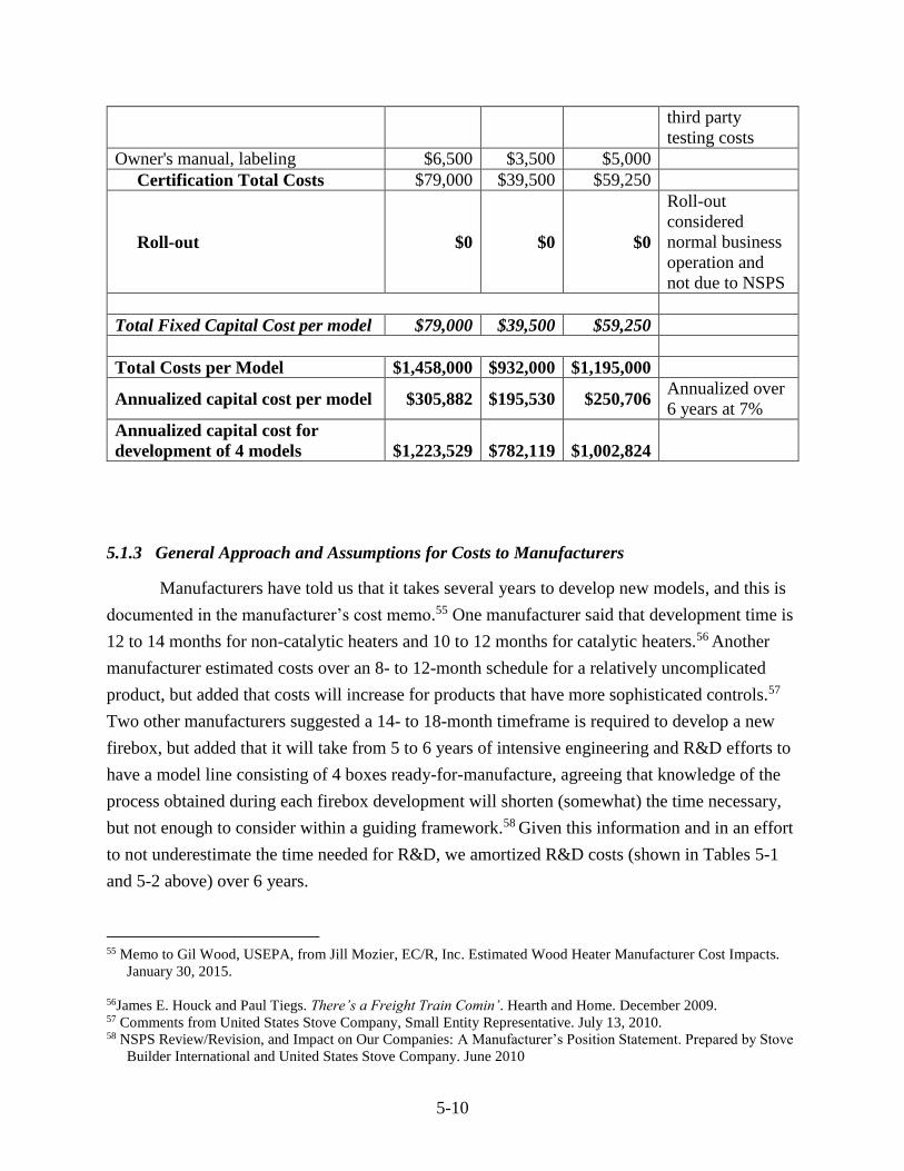
5-10
third party
testing costs
Owner's manual, labeling $6,500 $3,500 $5,000
Certification Total Costs $79,000 $39,500 $59,250
Roll-out $0 $0 $0
Roll-out
considered
normal business
operation and
not due to NSPS
Total Fixed Capital Cost per model $79,000 $39,500 $59,250
Total Costs per Model $1,458,000 $932,000 $1,195,000
Annualized capital cost per model $305,882 $195,530 $250,706 Annualized over
6 years at 7%
Annualized capital cost for
development of 4 models $1,223,529 $782,119 $1,002,824
5.1.3 General Approach and Assumptions for Costs to Manufacturers
Manufacturers have told us that it takes several years to develop new models, and this is
documented in the manufacturer’s cost memo.55 One manufacturer said that development time is
12 to 14 months for non-catalytic heaters and 10 to 12 months for catalytic heaters.56 Another
manufacturer estimated costs over an 8- to 12-month schedule for a relatively uncomplicated
product, but added that costs will increase for products that have more sophisticated controls.57
Two other manufacturers suggested a 14- to 18-month timeframe is required to develop a new
firebox, but added that it will take from 5 to 6 years of intensive engineering and R&D efforts to
have a model line consisting of 4 boxes ready-for-manufacture, agreeing that knowledge of the
process obtained during each firebox development will shorten (somewhat) the time necessary,
but not enough to consider within a guiding framework.58 Given this information and in an effort
to not underestimate the time needed for R&D, we amortized R&D costs (shown in Tables 5-1
and 5-2 above) over 6 years.
55 Memo to Gil Wood, USEPA, from Jill Mozier, EC/R, Inc. Estimated Wood Heater Manufacturer Cost Impacts.
January 30, 2015.
56James E. Houck and Paul Tiegs. There’s a Freight Train Comin’. Hearth and Home. December 2009. 57 Comments from United States Stove Company, Small Entity Representative. July 13, 2010. 58 NSPS Review/Revision, and Impact on Our Companies: A Manufacturer’s Position Statement. Prepared by Stove
Builder International and United States Stove Company. June 2010

5-11
We have assume that many manufacturers have already begun R&D efforts in
anticipation of the rule whose initial development was publicly announced by EPA in November
2009. However, for purposes of our cost estimate, we amortized the model development costs
(shown in Tables 5-1 and 5-2) over the 6 year period beginning in 2015 and ending in 2020
(inclusive). We prepared estimates using both a 7% interest rate and a 3% interest rate during the
amortization period.59
We estimated both the average annual cost to manufacturers of each appliance type and
then extended those costs to nationwide total annual costs. The basic components to each
manufacturer’s estimated annual cost are:
Annualized R&D cost;
Ongoing annual Certification cost; and
Ongoing annual Reporting and Record Keeping cost.
The Annualized R&D costs (shown in Tables 5-1 and 5-2) are by far the largest cost
component and we have applied these costs to most models in each appliance category –
especially to models in previously unregulated appliance categories and for appliances without a
voluntary program — in order to present an estimate of what might happen and avoid
underestimating cost impacts. For these appliances (i.e., single burn rate stoves and forced-air
furnaces), we estimated that 100% of the existing models will undergo R&D beginning in 2015
to meet the final limits. In cases where we assumed less than 100% of the models would require
R&D (e.g., adjustable burn rate stoves, pellet stoves and hydronic heaters), this was based on the
percentage of models estimated to already meet the 2020 Step 2 limit, as explained above.
However, it is important to note that manufacturers will likely consolidate their model
lines, focusing on models able to achieve the limit, rather than incur R&D costs for every
currently non-compliant model line. Therefore fewer models than we used in our cost estimates
will likely undergo R&D, which will decrease cost impacts, potentially significantly. But since
we do not have data to suggest the degree of consolidation which may occur, we assumed all
non-compliant models would remain in existence and incur R&D costs, in order to avoid
underestimating costs.
59 See January 2015 cost effectiveness (CE) spreadsheets including for PM2.5 the Revised Final Wood Heater NSPS
PM CE 7% and the Revised Final Wood Heater NSPS PM CE 3% for the CE analysis supporting the NSPS. All
of these spreadsheets are found in the public docket for this rulemaking.

5-12
Furthermore, for appliances like single burn rate stoves and forced air furnaces, which
were previously unregulated (and also were not pushed technologically by a voluntary program,
as hydronic heaters were), we have doubled the R&D/Engineering cost portion of the total costs
in the first 2 years (2014 and 2015). This doubling of the R&D/Engineering costs represents an
intensification of the R&D efforts to meet the Step 1 limit and begin development of models to
meet the Step 2 limit – R&D efforts which industry has indicated are already ongoing.60
All manufacturers, except for wood stoves that are subject to the existing 1988 NSPS
(and therefore already incur certification costs), will face ongoing certification costs above
baseline conditions. In the 2015 to 2020 time frame, we have incorporated these costs as part of
the overall R&D expenditures. For the purposes of our analysis, which estimates initial R&D
costs from 2015 to 2020 and ongoing costs for bringing a model to market after 2020, the
ongoing certification and reporting and recordkeeping costs faced by manufacturers are
estimated over the 10-year model lifespan.61,62
Regarding ongoing certification costs (after initial certification which is estimated in the R&D
costs itemized above in Tables 5-1 and 5-2), we estimated a continuing cost of $10,000 per
model for pellet stoves and single burn rate stoves and a continuing cost of $20,000 per model
for hydronic heaters and forced air furnaces.63 We distributed these ongoing costs out over the 5
year certification life, assuming annual certification costs for one-fifth of the models. For
example, compliant (but as yet uncertified) pellet stoves will incur certification costs in 2015. As
explained in the manufacturer’s cost memo,64 approximately 70% of existing pellet stove models
are expected to comply with the Step 2 PM standard without requiring intensive R&D. However,
in order to be sold, these stove models would now be required to demonstrate compliance with
an emissions limit, incurring an upfront cost of $10,000 per model to become certified. We have
estimated that one fifth of the pellet stove models will certify in any given year.
We based reporting and recordkeeping (R&R) costs on the annual average costs derived
from development of the Information Collection Request (ICR) supporting statements.65 These
60 February 8, 2013 telephone discussion between Gil Wood, USEPA, and a manufacturer of forced air furnaces and
single burn rate stoves. 61 Memorandum to USEPA from EC/R, Inc. Estimated Emissions from Wood Heaters. January 2015. 62 Memorandum to USEPA from EC/R, Inc. Residential Wood Heater Cost Effectiveness Analysis. January 2015. 63 Conversation with Dennis Brazier, Central Boiler. August 9, 2010. 64 Memo to Gil Wood, USEPA, from Jill Mozier, EC/R, Inc. Estimated Wood Heater Manufacturer Cost Impacts.
January 30, 2015. 65Memo to David Cole, Gil Wood and Amanda Aldridge, USEPA, from Joanne O’Loughlin, EC/R, Inc. Estimated
Reporting and Recordkeeping Costs Itemized for Cost Effectiveness Analysis. January 30, 2015.

5-13
are annual estimates of the ongoing R&R burden to manufacturers associated with final rule
compliance. We estimate that R&R costs are incurred beginning in 2015 in our analysis.
As noted above, the certification and reporting and recordkeeping costs were estimated to
be incurred by manufacturers for the full 10-year model design lifespan, for models designed to
meet each final limit.66 We therefore estimated costs from 2015 through 2029—that is, 10 years
after the 2020 compliance year marking the beginning of the model lifespan designed to meet the
Step 2 PM emission limit. We provide these costs in the manufacturer’s cost memo.
5.1.4. Estimated Manufacturer Costs – Specific Assumptions & Resulting Costs
Below is a list of approach and assumptions for estimating costs for each category of
appliances affected by this final rule, as taken from the manufacturer cost memo.67 Costs vary
by appliance type based on the estimated number of models. Our estimates of the number of
models for each appliance type are described in the unit cost memo.68 For numbers of
manufacturers, we started with HPBA data and modified those numbers as needed, based on
internet searches of manufacturers of the major appliance types.69
1. Nationwide Annual Cost assumes R&D investment is amortized over 6 years (2015
through 2020). Ongoing certification costs are incurred through 2029 (based on a
model brought to market in 2020 with a lifespan of 10 years).
2. Since certification is required every 5 years, it is assumed that certification costs will
be spread out so that 1/5 of the models certify each year.
3. This analysis considers additional costs resulting from the NSPS. For wood stoves,
the analysis assumes that 26% meet Step 2 already so that 74% of the models will
undergo re-design to meet the Step 2 limit. The costs modeled for years 2021 through
2029 exclude the ongoing certification costs and ongoing reporting and recordkeeping
costs incurred by wood stove manufacturers who already had to certify and report
under the existing 1988 NSPS.
4. For pellet stoves, the analysis assumes that 70% meet Step 2 already so that 30% of
models undergo R&D re-design to meet Step 2. The R&D budget includes
certification costs. The analysis also assumes that the 70% of the pellet stove models
66 Memo to Gil Wood, USEPA, from Jill Mozier, EC/R, Inc. Unit Cost Estimates of Residential Wood Heating
Appliances. January 30, 2015. 67 Memo to Gil Wood, USEPA, from Jill Mozier, EC/R, Inc. Estimated Wood Heater Manufacturer Cost Impacts.
January 30, 2015.
68 Memorandum to USEPA from EC/R, Inc. Unit Cost Estimates of Residential Wood Heating Appliances. January
30, 2015. 69 HPBA Solid Fuel Product List. Attachment to E-mail from John Crouch, HBPS, to Gil Wood, EPA. September
24, 2010.

5-14
that already meet Step 2 will certify in an ongoing basis starting in 2015. The analysis
reflects the certification costs beginning in 2015 for the 70% of models meeting Step
2, and beginning in 2020 for the remaining 30% of models which underwent R&D re-
design. The analysis also reflects ongoing reporting and recordkeeping costs for
100% of the models beginning in 2015.
5. Based on conversations with industry, single burn rate stoves and forced air furnaces
have been undergoing R&D prior to 2014 to develop cleaner models. Because these
devices were previously unregulated and may need to transfer technology from
adjustable burn rate stoves and hydronic heaters, respectively, this analysis assumes
that these efforts will intensify in 2015 and 2016. Therefore estimated R&D costs are
doubled in 2015 and 2016 to reflect model development to meet the more stringent
2020 Step 2 PM emission limit.
6. For single burn rate stoves and forced air furnaces, the analysis assumes that only a
small percentage meet Step 2 so that approximately 100% of the models undergo
R&D re-design to meet Step 2. The R&D budget includes certification costs. Ongoing
certification costs for the re-designed models are reflected in this analysis beginning
in 2021. Ongoing reporting & recordkeeping for all models are estimated beginning
in 2015.
7. Reporting and recordkeeping costs (R&R) are based on the annual average costs
derived from the ICR and are estimates of the ongoing R&R burden to manufacturers
associated with the NSPS. The annual average nationwide R&R burden estimated to
manufacturers for Subpart AAA is $179,000 for years 2015 through 2017, and
$352,000 for years 2018 through 2020. For Subpart QQQQ, the R&R burden to
manufacturers is $141,000 for years 2015 through 2017, and $197,000for years 2018
through 2020. Although the 2018 through 2020 costs are carried forward to 2029 for
this analysis, actual R&R costs from 2021 through 2029 may vary slightly. These
R&R costs do not include the R&R burden to laboratories and certifying entities,
which have been calculated separately.
8. For hydronic heaters, the analysis assumes that 18% of models meet Step 2 already
so that the remaining 82% must undergo R&D to meet Step 2 in 2020. The R&D
budget includes certification costs. Ongoing certification costs for the re-designed
models are reflected in this analysis beginning in 2021. Ongoing reporting &
recordkeeping for all models are estimated beginning in 2015.
Table 5-3 provides the average annual cost per manufacturer under the final NSPS. The
costs in the table vary by appliance type based on the average number of models per
manufacturer. The estimate of the number of model types are described in the unit cost memo.70
70 Memo to Gil Wood and David Cole, US EPA, from Beth Friedman, EC/R, Inc. Unit Cost Estimates of Residential
Wood Heating Appliances. January 30, 2015.

5-15
For numbers of manufacturers, we started with HPBA data, modified based on internet searches
of manufacturers of the major appliance types.71
The following example explains how the average annual cost in Table 5-3 is estimated
for hydronic heater manufacturers.
1) We derived the annualized capital cost per model for R&D related costs including
certification based on industry-supplied cost components as described on pages 5-7 to 5-
10 of the RIA. The estimated annualized capital cost to bring a hydronic heater (HH)
model through R&D, based on an amortization period of 6 years and an interest rate of
7%, is $250,706.
2) To derive the average annual cost to each HH manufacturer, we multiplied the annualized
capital cost of $250,706 by the estimated number of Hydronic Heater models in the
nation, 120, divided by the estimated number of HH manufacturers, 30. As stated above,
the numbers of models and manufacturers were derived from an industry-supplied list of
manufacturers by product type with additional refining via internet searches and EPA’s
experience with the HH voluntary program.
3) To refine the average annual cost further, we estimated the percentage of HH models that
already meet the Step 2 PM emission limit – and therefore would not need to incur R&D
costs, but only certification and reporting & recordkeeping (R&R) costs. This percentage
is based on the qualifying emissions data in the current EPA-HH Voluntary Program
database. We estimate that 18% of current HH models can meet Step 2 without
additional R&D. Therefore 82% of HH models will incur R&D, certification and
reporting and recordkeeping costs; while 18% of HH models will incur only certification
and reporting and recordkeeping costs.
4) We estimate ongoing HH certification testing (outside the R&D process) to cost $20,000
per certification. This $20,000 figure is supplied by industry. Since a certification is
good for 5 years, in order to determine an annual certification cost, we assumed that
manufacturers will choose to spread out certification costs by certifying one-fifth of their
models each year. (Note again that the certification cost for models undergoing R&D is
included in the $250,706 R&D cost).
5) We estimated ongoing HH (R&R) costs based on Information Collection Request (ICR)
assumptions, which were calculated for the first 3 years and then for the 3 years
following, respectful of changing R&R costs to meet a 2-Step standard. R&R costs are
based on the annual average costs derived from the ICR and are estimates of the ongoing
R&R burden to manufacturers associated with the NSPS. The annual average R&R
71 HPBA Solid Fuel Product List. Attachment to E-mail from John Crouch, HBPA, to Gil Wood, US EPA.
September 24, 2010.
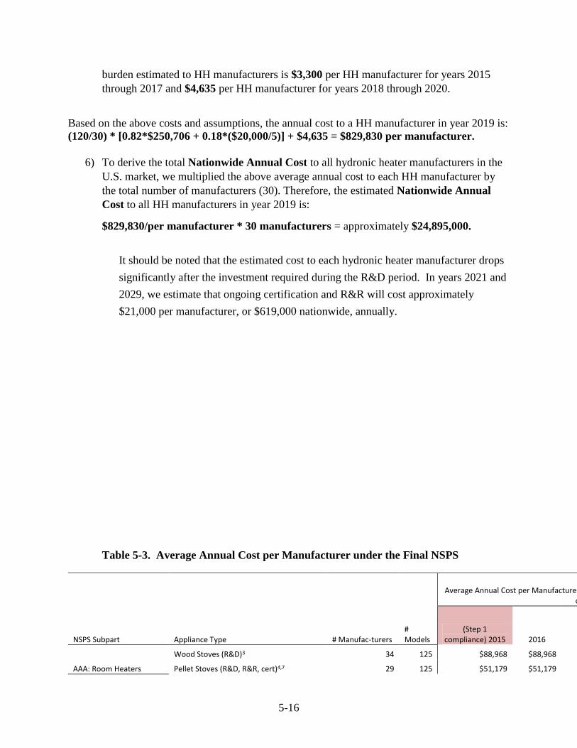
5-16
burden estimated to HH manufacturers is $3,300 per HH manufacturer for years 2015
through 2017 and $4,635 per HH manufacturer for years 2018 through 2020.
Based on the above costs and assumptions, the annual cost to a HH manufacturer in year 2019 is:
(120/30) * [0.82*$250,706 + 0.18*($20,000/5)] + $4,635 = $829,830 per manufacturer.
6) To derive the total Nationwide Annual Cost to all hydronic heater manufacturers in the
U.S. market, we multiplied the above average annual cost to each HH manufacturer by
the total number of manufacturers (30). Therefore, the estimated Nationwide Annual
Cost to all HH manufacturers in year 2019 is:
$829,830/per manufacturer * 30 manufacturers = approximately $24,895,000.
It should be noted that the estimated cost to each hydronic heater manufacturer drops
significantly after the investment required during the R&D period. In years 2021 and
2029, we estimate that ongoing certification and R&R will cost approximately
$21,000 per manufacturer, or $619,000 nationwide, annually.
Table 5-3. Average Annual Cost per Manufacturer under the Final NSPS
NSPS Subpart Appliance Type # Manufac-turers # Models
Average Annual Cost per Manufacturer based on 6-year R&D round (2015-2020) to meet Step 1 and Step 2 limits with ongoing certification costs (through 2029)
(Step 1 compliance) 2015 2016 2017 2018 2019
(Step 2 compliance) 2020
2021 through 20292
AAA: Room Heaters
Wood Stoves (R&D)3 34 125 $88,968 $88,968 $88,968 $88,968 $88,968 $88,968 $0
Pellet Stoves (R&D, R&R, cert)4,7 29 125 $51,179 $51,179 $51,179 $53,941 $53,941 $53,941 $14,240
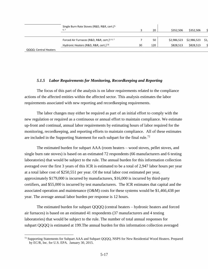
5-17
Single Burn Rate Stoves (R&D, R&R, cert.)5,
6, 7 3 20 $352,506 $352,506 $352,506 $226,704 $226,704 $226,704 $22,025
QQQQ: Central Heaters
Forced Air Furnaces (R&D, R&R, cert.)5, 6, 7 7 50 $2,986,523 $2,986,523 $1,796,681 $1,799,034 $1,799,034 $1,799,034 $36,849
Hydronic Heaters (R&D, R&R, cert.)7,8 30 120 $828,513 $828,513 $828,513 $829,831 $829,831 $829,831 $20,635
5.1.5 Labor Requirements for Monitoring, Recordkeeping and Reporting
The focus of this part of the analysis is on labor requirements related to the compliance
actions of the affected entities within the affected sector. This analysis estimates the labor
requirements associated with new reporting and recordkeeping requirements.
The labor changes may either be required as part of an initial effort to comply with the
new regulation or required as a continuous or annual effort to maintain compliance. We estimate
up-front and continual, annual labor requirements by estimating hours of labor required for the
monitoring, recordkeeping, and reporting efforts to maintain compliance. All of these estimates
are included in the Supporting Statement for each subpart for the final rule.72
The estimated burden for subpart AAA (room heaters – wood stoves, pellet stoves, and
single burn rate stoves) is based on an estimated 72 respondents (66 manufacturers and 6 testing
laboratories) that would be subject to the rule. The annual burden for this information collection
averaged over the first 3 years of this ICR is estimated to be a total of 2,947 labor hours per year
at a total labor cost of $250,551 per year. Of the total labor cost estimated per year,
approximately $179,000 is incurred by manufacturers, $16,000 is incurred by third-party
certifiers, and $55,000 is incurred by test manufacturers. The ICR estimates that capital and the
associated operation and maintenance (O&M) costs for these systems would be $1,466,438 per
year. The average annual labor burden per response is 12 hours.
The estimated burden for subpart QQQQ (central heaters – hydronic heaters and forced
air furnaces) is based on an estimated 41 respondents (37 manufacturers and 4 testing
laboratories) that would be subject to the rule. The number of total annual responses for
subpart QQQQ is estimated at 199.The annual burden for this information collection averaged
72 Supporting Statements for Subpart AAA and Subpart QQQQ, NSPS for New Residential Wood Heaters. Prepared
by EC/R, Inc. for U.S. EPA. January 30, 2015.

5-18
over the first 3 years of this ICR is estimated to be a total of 2,337 labor hours per year at a total
labor cost of $191,904 per year. Of the total labor cost estimated per year, approximately
$140,000 is incurred by manufacturers, $15,000 is incurred by third-party certifiers, and $36,000
is incurred by test manufacturers. The ICR estimates that capital and operation and maintenance
(O&M) costs would be $3,191,188 per year. The average annual labor burden per response is 12
hours.
We note that certification testing (once every 5 years unless a waiver is granted) costs of
approximately $10,000 ($20,000 for hydronic heaters and forced air furnaces) per model line in
2021 result in labor hours spent at the test lab, which are not included in this labor rate analysis.
In addition, each model that is developed (i.e., number of affected units) will face an annual
estimated cost of $160,000 for the salaries of two full-time experimental employees for 5 years.
This estimate should be regarded as a partial labor estimate, with other possible labor associated
with new model development (such as re-tooling) left as unquantified and described qualitatively
in the manufacturer cost and unit cost impact memos.
Ongoing monitoring, recordkeeping, and reporting labor requirements for the final rule
are estimated at about 5,300 hours per year.73 These ongoing labor requirements can be viewed
as average sustained labor requirements required for affected entities to continuously comply
with the new regulations in 2020 and beyond.
5.2 Compliance Costs of the Rule as Presented in the RIA
EPA’s engineering cost analysis estimates that the total annualized cost, which includes
all compliance costs associated with the regulation, to manufacturers as presented in this RIA is
$45.7 million, calculated as an average of the annualized costs incurred from 2015 to 2020 (all
costs are reported in 2013 dollars) (EC/R, August 2014). Annualized costs are estimated at a 7%
interest rate.74 We calculate the costs in this way in order to provide an average of annualized
costs from the time of rule promulgation in 2015 to the time of full implementation which occurs
in 2020. Having an average annualized calculation for the costs allows for a reasonable measure
of the costs to be incurred by manufacturers given the changes in costs year by year between
73 Memo to Gil Wood, USEPA, from EC/R, Inc. Residential Wood Heating ICR Analysis.
January 30, 2015. 74 EC/R, Inc. to U.S. EPA, Memorandum. Estimated Residential Wood Heater Manufacturer Cost Impacts. January
30, 2015.

5-19
2015 and 2020 as shown in the manufacturer’s cost memo for this final rule. The total annualized
costs for each year and for each option are in Table 5-4.
With total annualized costs estimated at a 3% interest rate, the total annualized cost of the
rule is $40.2 million in 2013 dollars. More detailed information on the costs at a 3% interest rate
can be found in the cost memoranda for this final rule.
Under the NSPS, the costs in the 2015-2020 time frame fall most heavily on
manufacturers of hydronic heating systems (54%), followed by forced air furnaces (34%), then
by wood stoves (7%). The remaining 5% of the costs are distributed to pellet stove
manufacturers (3%), and manufacturers of single burn rate stoves (2%).
Table 5-4. Summary of Average Annualized Nationwide Costs for the 2015–2020 Time
Frame Under the Final NSPS
Appliance Type Final NSPS
Wood Heaters $3,020,000
Single Burn Rate Heaters $870,000
Pellet Stoves $1,520,000
Forced-Air Furnaces $15,360,000
Hydronic Heating Systems $24,880,000
Total Average Annual Cost for 2015–2020 Time Frame $45,660,000
The final rule, will affect an estimated 2.7 million new residential wood heating devices
between 2015 and 2020 assuming an average of ~296,000 new shipments annually as presented
in the emissions memo for the final rule.75 As shown previously in Table 4-4 in Section 4, annual
shipments are forecasted to increase for all product types over the same time period.
To assess the size of the compliance costs relative to the value of shipments to end-use
consumers, we compared industry-level compliance costs relative to projected sales over the
timeframe from 2015 to 2020. In this case, cost-to-receipts ratios approximate the maximum
price increase needed for a producer to fully recover the annual compliance costs associated with
a regulation. These industry-level cost-to-receipts ratios can be interpreted as an average impact
on potentially affected firms in these industries all other things equal, and where ratios less than
75 U.S. EPA. Memorandum. Estimated Emissions from Wood Heaters. January 30, 2015. Prepared by EC/R, Inc.
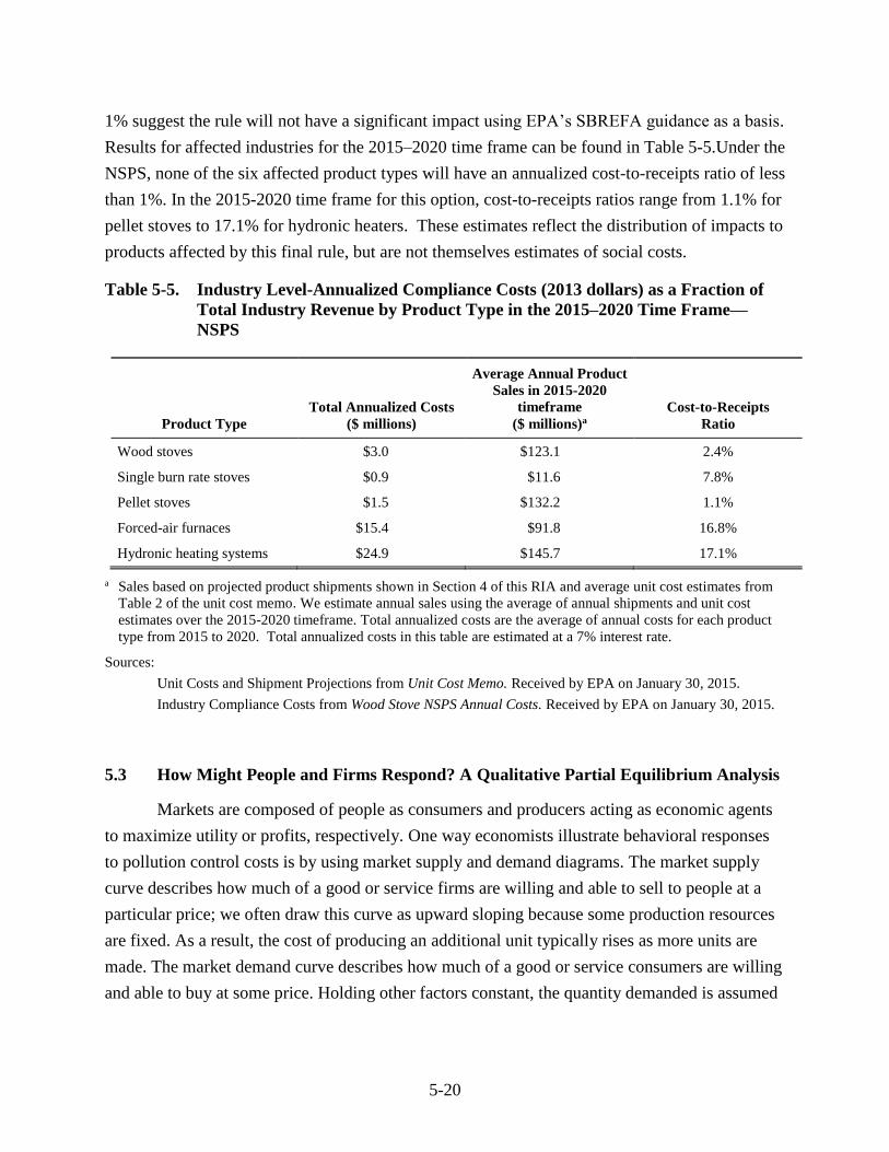
5-20
1% suggest the rule will not have a significant impact using EPA’s SBREFA guidance as a basis.
Results for affected industries for the 2015–2020 time frame can be found in Table 5-5.Under the
NSPS, none of the six affected product types will have an annualized cost-to-receipts ratio of less
than 1%. In the 2015-2020 time frame for this option, cost-to-receipts ratios range from 1.1% for
pellet stoves to 17.1% for hydronic heaters. These estimates reflect the distribution of impacts to
products affected by this final rule, but are not themselves estimates of social costs.
Table 5-5. Industry Level-Annualized Compliance Costs (2013 dollars) as a Fraction of
Total Industry Revenue by Product Type in the 2015–2020 Time Frame—
NSPS
Product Type
Total Annualized Costs
($ millions)
Average Annual Product
Sales in 2015-2020
timeframe
($ millions)a
Cost-to-Receipts
Ratio
Wood stoves $3.0 $123.1 2.4%
Single burn rate stoves $0.9 $11.6 7.8%
Pellet stoves $1.5 $132.2 1.1%
Forced-air furnaces $15.4 $91.8 16.8%
Hydronic heating systems $24.9 $145.7 17.1%
a Sales based on projected product shipments shown in Section 4 of this RIA and average unit cost estimates from
Table 2 of the unit cost memo. We estimate annual sales using the average of annual shipments and unit cost
estimates over the 2015-2020 timeframe. Total annualized costs are the average of annual costs for each product
type from 2015 to 2020. Total annualized costs in this table are estimated at a 7% interest rate.
Sources:
Unit Costs and Shipment Projections from Unit Cost Memo. Received by EPA on January 30, 2015.
Industry Compliance Costs from Wood Stove NSPS Annual Costs. Received by EPA on January 30, 2015.
5.3 How Might People and Firms Respond? A Qualitative Partial Equilibrium Analysis
Markets are composed of people as consumers and producers acting as economic agents
to maximize utility or profits, respectively. One way economists illustrate behavioral responses
to pollution control costs is by using market supply and demand diagrams. The market supply
curve describes how much of a good or service firms are willing and able to sell to people at a
particular price; we often draw this curve as upward sloping because some production resources
are fixed. As a result, the cost of producing an additional unit typically rises as more units are
made. The market demand curve describes how much of a good or service consumers are willing
and able to buy at some price. Holding other factors constant, the quantity demanded is assumed

5-21
to fall when prices rise. In a perfectly competitive market, equilibrium price (P0) and quantity
(Q0) are determined by the intersection of the supply and demand curves (see Figure 5-2).
5.3.1 Changes in Market Prices and Quantities
To qualitatively assess how the regulation may influence the equilibrium price and
quantity in the affected markets, we assumed the market supply function shifts up by the
additional cost of producing the good or service; the unit cost increase is typically calculated by
dividing the annual compliance cost estimate by the baseline quantity (Q0) (see Figure 5-2). As
shown, this model makes two predictions: the price of the affected goods and services are likely
to rise and the consumption/production levels are likely to fall.
The size of these changes depends on two factors: the size of the unit cost increase
(supply shift) and differences in how each side of the market (supply and demand) responds to
changes in price. Economists measure responses using the concept of price elasticity, which
represents the percentage change in quantity divided by the percentage change in price. This
dependence has been expressed in the following formula:76
Demand) of Elasticity Price - Supply of Elasticity Price
Supplyof Elasticity Priceuniter-Share of p cost
As a general rule, a higher share of the per-unit cost increases will be passed on to
consumers in markets where
goods and services are necessities and people do not have good substitutes that they
can switch to easily (demand is inelastic) and
suppliers have excess capacity and can easily adjust production levels at minimal
costs, or the time period of analysis is long enough that suppliers can change their
fixed resources; supply is more elastic over longer periods.
76 For examples of similar mathematical models in the public finance literature, see Nicholson (1998), pages 444–
447, or Fullerton and Metcalf (2002).
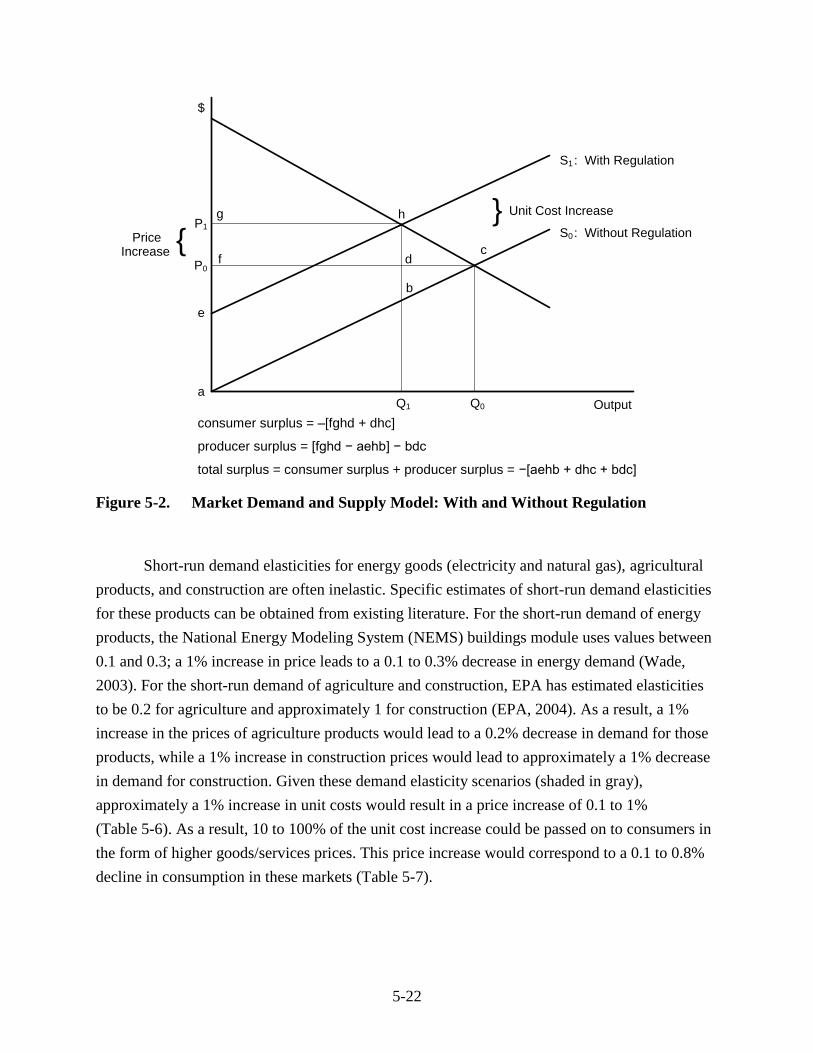
5-22
consumer surplus = –[fghd + dhc]
producer surplus = [fghd − aehb] − bdc
total surplus = consumer surplus + producer surplus = −[aehb + dhc + bdc]
Figure 5-2. Market Demand and Supply Model: With and Without Regulation
Short-run demand elasticities for energy goods (electricity and natural gas), agricultural
products, and construction are often inelastic. Specific estimates of short-run demand elasticities
for these products can be obtained from existing literature. For the short-run demand of energy
products, the National Energy Modeling System (NEMS) buildings module uses values between
0.1 and 0.3; a 1% increase in price leads to a 0.1 to 0.3% decrease in energy demand (Wade,
2003). For the short-run demand of agriculture and construction, EPA has estimated elasticities
to be 0.2 for agriculture and approximately 1 for construction (EPA, 2004). As a result, a 1%
increase in the prices of agriculture products would lead to a 0.2% decrease in demand for those
products, while a 1% increase in construction prices would lead to approximately a 1% decrease
in demand for construction. Given these demand elasticity scenarios (shaded in gray),
approximately a 1% increase in unit costs would result in a price increase of 0.1 to 1%
(Table 5-6). As a result, 10 to 100% of the unit cost increase could be passed on to consumers in
the form of higher goods/services prices. This price increase would correspond to a 0.1 to 0.8%
decline in consumption in these markets (Table 5-7).
Q1 Q0
P1
P0
h
c
a
$
Output
e
d
S1 : With Regulation
S0 : Without RegulationPriceIncrease
}
Unit Cost Increase}g
f
b
5-23
For this final rule, a commenter on the proposed rule provided an estimate of -0.97 for the
price elasticity of demand for hydronic heaters. 77 The commenter also provided estimates of
changes in price and output for hydronic heater as part of their report. However, the
commenter’s analysis presumed an inelastic (or flat) supply curve, which presumes no
responsiveness of producers to a change in product price. EPA does not have estimates of the
price elasticity of supply, an essential value in order to accurately estimate impacts of appliance
supply and demand. In addition, the price elasticity of demand provided by the commenter is
specific to data for this appliance category and not other appliance categories covered by this
final rule. Thus, EPA does not estimate price and output changes using partial equilibrium
techniques for wood-burning appliance producers and consumers affected by this final rule.
While we are unable to estimate price and output changes, we note that the high increases in unit
costs for some affected appliances could lead to potential nontrivial increases in market price to
wood-burning appliance consumers and potential decreases in output for such appliances if
supply elasticities are determined to be low. This could be true for hydronic heaters and forced
air furnaces, but is unlikely for wood stoves and pellet stoves.
As for using other economic impact modeling approaches such as computable general
equilibrium (CGE) modeling, which was used in the Transport Rule proposed in the summer of
2010 and in other rulemakings over the last several years, EPA used the Economic Model for
Policy Analysis (EMPAX) to estimate the effect of impacts on markets outside of the regulated
sector. EMPAX is a dynamic computable general equilibrium model (CGE) which forecasts a
new equilibrium for the entire economy after a policy intervention. However, since the
Transport Rule was proposed, an updated version of EMPAX was used to estimate the social
cost of the Clean Air Act in an EPA report entitled “The Benefits and Costs of the Clean Air Act
from 1990 to 2020.” This report is available at
http://www.epa.gov/air/sect812/feb11/fullreport.pdf. This updated version of EMPAX added in
the benefit-side effects (incorporating labor-force and health care expenditures) which
significantly changed the social cost estimate from the previous edition. In December 2010,
EPA’s Science Advisory Board (SAB)’s external Council on Clean Air Compliance Analysis
(hereafter “Council”) peer review of this EPA report stated found that inclusion of benefit-side
effects, specifically adapted for use in that study, “represent[ed] a significant step forward in
benefit-cost analysis,” While the Council has made this finding, EPA recognizes that serious
technical challenges remain when attempting to evaluate the benefits and costs of potential
regulatory actions using economy-wide models. Consistent with the Council’s advice regarding
77 NERA. Cost-Effectiveness Analysis of Alternative Hydronic Heater New Source Performance Standards. May
2014. Prepared for the Hearth, Barbecue, and Patio Association.
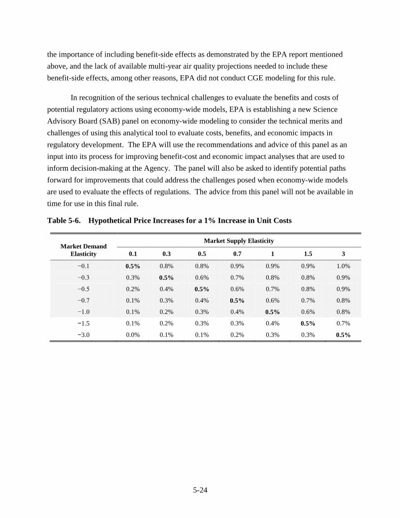
5-24
the importance of including benefit-side effects as demonstrated by the EPA report mentioned
above, and the lack of available multi-year air quality projections needed to include these
benefit-side effects, among other reasons, EPA did not conduct CGE modeling for this rule.
In recognition of the serious technical challenges to evaluate the benefits and costs of
potential regulatory actions using economy-wide models, EPA is establishing a new Science
Advisory Board (SAB) panel on economy-wide modeling to consider the technical merits and
challenges of using this analytical tool to evaluate costs, benefits, and economic impacts in
regulatory development. The EPA will use the recommendations and advice of this panel as an
input into its process for improving benefit-cost and economic impact analyses that are used to
inform decision-making at the Agency. The panel will also be asked to identify potential paths
forward for improvements that could address the challenges posed when economy-wide models
are used to evaluate the effects of regulations. The advice from this panel will not be available in
time for use in this final rule.
Table 5-6. Hypothetical Price Increases for a 1% Increase in Unit Costs
Market Demand
Elasticity
Market Supply Elasticity
0.1 0.3 0.5 0.7 1 1.5 3
−0.1 0.5% 0.8% 0.8% 0.9% 0.9% 0.9% 1.0%
−0.3 0.3% 0.5% 0.6% 0.7% 0.8% 0.8% 0.9%
−0.5 0.2% 0.4% 0.5% 0.6% 0.7% 0.8% 0.9%
−0.7 0.1% 0.3% 0.4% 0.5% 0.6% 0.7% 0.8%
−1.0 0.1% 0.2% 0.3% 0.4% 0.5% 0.6% 0.8%
−1.5 0.1% 0.2% 0.3% 0.3% 0.4% 0.5% 0.7%
−3.0 0.0% 0.1% 0.1% 0.2% 0.3% 0.3% 0.5%

5-25
Table 5-7. Hypothetical Consumption Decreases for a 1% Increase in Unit Costs
Market Demand
Elasticity
Market Supply Elasticity
0.1 0.3 0.5 0.7 1 1.5 3
−0.1 −0.1% −0.1% −0.1% −0.1% −0.1% −0.1% −0.1%
−0.3 −0.1% −0.2% −0.2% −0.2% −0.2% −0.3% −0.3%
−0.5 −0.1% −0.2% −0.3% −0.3% −0.3% −0.4% −0.4%
−0.7 −0.1% −0.2% −0.3% −0.4% −0.4% −0.5% −0.6%
−1.0 −0.1% −0.2% −0.3% −0.4% −0.5% −0.6% −0.8%
−1.5 −0.1% −0.3% −0.4% −0.5% −0.6% −0.8% −1.0%
−3.0 −0.1% −0.3% −0.4% −0.6% −0.8% −1.0% −1.5%
5.3.2 Partial Equilibrium Measures of Social Cost: Changes in Consumer and Producer
Surplus
In partial equilibrium analysis, the social costs are estimated by measuring the changes in
consumer and producer surplus, and these values can be determined using the market supply and
demand model (as shown in Figure 5-2). Assuming linear market supply and demand curves as
shown in Figure 5-2, the change in consumer surplus (CS) is measured as follows:
CS = − [Q1 × p] + [0.5 × Q × p]. (5.1)
where a coefficient of 0.5 is multiplied to the change in Q and P resulting from the shock
to the markets based on the assumption of linear demand and supply curves in the diagram
above and applying principles of basic geometry. Higher market prices and lower quantities lead
to consumer welfare losses. Similarly, the change in producer surplus (PS) is measured as
follows for affected supply:
PS = [Q1 × p] − [Q1 × t] − [0.5 × Q × (p − t)]. (5.2)
Where t = per unit cost increase. Higher unit costs and lower production levels reduce producer
surplus because the net price change (p − t) is negative. However, these losses are mitigated
because market prices tend to rise. In contrast, for unaffected supply, the change in producer
surplus is:
PS = [Q0 × p] + [0.5 × Q × p]. (5.3)
5-26
Higher prices increase producer surplus for unaffected producers in the U.S. and other
countries.
5.4 Social Cost Estimate
As shown in Table 5-6, the social cost as approximated by the annual compliance costs as
a percent of sales represent a fraction of the affected product value that is greater than 1% for
each of the product categories; this suggests that the shift of the supply curve may be relatively
large for some product types and result in larger changes in market prices and consumption.
However, lacking information on the shift of affected supply curves and related price elasticities
of supply, EPA believes the national annualized compliance cost estimates provide a reasonable
approximation of the social cost of this rule. EPA believes this approximation is better for
industries whose markets are well characterized as perfectly competitive. However, given the
data limitations noted earlier, EPA believes the accounting for annual compliance costs is a
reasonable approximation to inform policy discussion in this rulemaking. We were not able to
prepare a full economic analysis of the impacts of this proposal on supply and demand, or the
effects of such impacts on emissions (e.g. feedback effect on emissions). Most of the affected
industries can be characterized as having a high degree of competitive market behavior as
described in Section 3 of this RIA. To shed more light on the level of market behavior, EPA ran
hypothetical economic impact analyses and the results are in Tables 5-6 and 5-7.
5.5 Energy Impacts
Executive Order 13211 (66 FR 28355, May 22, 2001) provides that agencies will prepare
and submit to the Administrator of the Office of Information and Regulatory Affairs, Office of
Management and Budget, a Statement of Energy Effects for certain actions identified as
“significant energy actions.” Section 4(b) of Executive Order 13211 defines “significant energy
actions” as any action by an agency (normally published in the Federal Register) that
promulgates or is expected to lead to the promulgation of a final rule or regulation, including
notices of inquiry, advance notices of proposed rulemaking, and notices of proposed rulemaking:
(1) (i) that is a significant regulatory action under Executive Order 12866 or any successor order,
and (ii) is likely to have a significant adverse effect on the supply, distribution, or use of energy;
or (2) that is designated by the Administrator of the Office of Information and Regulatory Affairs
as a significant energy action.
This final rule is not a “significant energy action” as defined in Executive Order 13211
(66 FR 28355, May 22, 2001), because it is not likely to have a significant adverse effect on the
supply, distribution, or use of energy. Further, we have concluded that this rule is not likely to

5-27
have any significant adverse energy effects. In general, we expect the NSPS to improve
technology, including energy efficiency. Reducing emissions and increasing efficiency might
increase the use of wood fuel, which would relieve pressure on traditional coal or petroleum
based energy sources. However, as described in section VI.E of the preamble, it is difficult to
determine the precise energy impacts that might result from this rule. This is because wood-
fueled appliances compete with other biomass forms as well as more traditional oil, electricity
and natural gas. Robust data are not available to determine the potential conversion to other types
of fuels and their associated appliances if the consumer costs of wood-fueled appliances increase
and at what level that increase would drive consumer choice.
5.6 Unfunded Mandates Reform Act (UMRA)
5.6.1 Future and Disproportionate Costs
The UMRA requires that we estimate, where accurate estimation is reasonably feasible,
future compliance costs imposed by the rule and any disproportionate budgetary effects. Our
estimates of the future compliance costs of the rule are discussed previously in this RIA. The
nationwide annualized average compliance cost of this rule for directly affected appliances is
$45.7 million in the 2015-2020 time frame (2013 dollars). Therefore, this rule is not subject to
the requirements of Sections 202 or 205 of the UMRA.
This rule is not subject to the requirements of Section 203 of UMRA because it contains
no regulatory requirements that might significantly or uniquely affect small governments. The
rule would not apply to such governments and would impose no obligations upon them.
5.6.2 Effects on the National Economy
The UMRA requires that we estimate the effect of the rule on the national economy. To
the extent feasible, we must estimate the effect on productivity, economic growth, full
employment, creation of productive jobs, and international competitiveness of U.S. goods and
services if we determine that accurate estimates are reasonably feasible and that such effect is
relevant and material. The nationwide economic impact of the rule is presented earlier in this
RIA chapter. This analysis provides estimates of the effect of the rule on most of the categories
mentioned above, and these estimates are presented earlier in this RIA chapter. The nature of this
rule is such that it is not practical for us to use existing approaches, such as the Morgenstern et
5-28
al. approach,78 to estimate the impact on employment to the regulated entities and others from
this rule. We explain why this is true, and provide impacts associated with the monitoring,
recordkeeping, and reporting requirements to provide some understanding of what impacts this
will have on employment for affected firms in section 5.7 below.
5.6.3 Executive Order 13045: Protection of Children from Environmental Health Risks and
Safety Risks
Executive Order 13045, “Protection of Children from Environmental Health Risks and
Safety Risks” (62 FR 19885, April 23, 1997), applies to any rule that: (1) is determined to be
“economically significant,” as defined under Executive Order 12866, and (2) concerns an
environmental health or safety risk that EPA has reason to believe may have a disproportionate
effect on children. If the regulatory action meets both criteria, EPA must evaluate the
environmental health or safety effects of the planned rule on children and explain why the
planned regulation is preferable to other potentially effective and reasonably feasible alternatives
considered by the Agency.
This rule is not subject to Executive Order 13045 (62 FR 19885, April 23, 1997) because
the Agency does not believe the environmental health risks or safety risks addressed by this
action present a disproportionate risk to children. The report, “Analysis of Exposure to
Residential Wood Combustion Emissions for Different Socio-Economic Groups,” 79shows that
on a nationwide basis, cancer risks due to residential wood smoke emissions among
disadvantaged population groups generally are lower than the risks for the general population
due to residential wood smoke emissions. One of the demographic variables examined for this
report was that of children 18 years and younger.
This final rule is expected to reduce environmental impacts for everyone, including
children. This action promulgates emissions limits at the levels based on the best system of
emissions reduction (BSER), as required by the Clean Air Act. Based on our analysis, we believe
that this rule would not have a disproportionate impact on children, and, in fact, will result in
improvements to children’s health. These emissions happen in neighborhoods and affect people
in their homes. To the extent that children are particularly sensitive to asthma, this rule will help.
78 Morgenstern, R. D., W. A. Pizer, and J. S. Shih. 2002. “Jobs versus the Environment: An Industry-Level
Perspective.” Journal of Environmental Economics and Management 43(3):412-436. 79 “Analysis of Exposure to Residential Wood Combustion Emissions for Different Socio-Economic Groups,
Revised Draft Report.” Prepared for Gil Wood, U.S. EPA, Office of Air Quality Planning and Standards,
Research Triangle Park, NC. Prepared by EC/R Inc., EPA Contract No. EP-D-05-085, Work Assignment No. 4-
3. April 22, 2010.

5-29
5.6.4 Executive Order 12898: Federal Actions to Address Environmental Justice in Minority
Populations and Low-Income Populations
Executive Order 12898 (59 FR 7629 (Feb. 16, 1994)) establishes federal executive policy
on environmental justice. Its main provision directs federal agencies, to the greatest extent
practicable and permitted by law, to make environmental justice part of their mission by
identifying and addressing, as appropriate, disproportionately high and adverse human health or
environmental effects of their programs, policies, and activities on minority populations and low-
income populations in the United States. The EPA defines “Environmental Justice” to include
meaning involvement of all people regardless of race, color, national origin, or income with
respect to the development, implementation and enforcement of environmental laws, regulations,
and polices.
As discussed in the proposal preamble, the report, “Analysis of Exposure to Residential
Wood Combustion Emissions for Different Socio-Economic Groups,” 80shows that on a
nationwide basis, cancer risks due to residential wood smoke emissions among disadvantaged
population groups generally are lower than the risks for the general population due to residential
wood smoke emissions. Thus, we have determined that this rule will not have disproportionately
high and adverse human health or environmental effects on minority, low-income or indigenous
populations because it increases the level of environmental protection for all affected populations
without having any disproportionately high and adverse human health or environmental effects
on any population, including any minority low-income or indigenous population.81 This rule
establishes national standards that will reduce primarily PM emissions from new residential
wood heaters and is expected to decrease the amount of these emissions to which all affected
populations are exposed. These emissions happen in minority and low-income neighborhoods
and affect people in their homes. To the extent that minority populations and low-income
populations are more vulnerable, this rule will help.
Although Executive Order 12898 focuses on human health and environmental impacts,
commenters on the proposed rule noted that wood heaters are purchased less frequently by low-
income groups than other income groups.
80 “Analysis of Exposure to Residential Wood Combustion Emissions for Different Socio-Economic Groups,
Revised Draft Report.” Prepared for Gil Wood, U.S. EPA, Office of Air Quality Planning and Standards,
Research Triangle Park, NC. Prepared by EC/R Inc., EPA Contract No. EP-D-05-085, Work Assignment No. 4-
3. April 22, 2010. 81 “Analysis of Exposure to Residential Wood Combustion Emissions for Different Socio-Economic Groups,
Revised Draft Report.” Prepared for Gil Wood, U.S. EPA, Office of Air Quality Planning and Standards,
Research Triangle Park, NC. Prepared by EC/R Inc., EPA Contract No. EP-D-05-085, Work Assignment No. 4-
3. April 22, 2010.
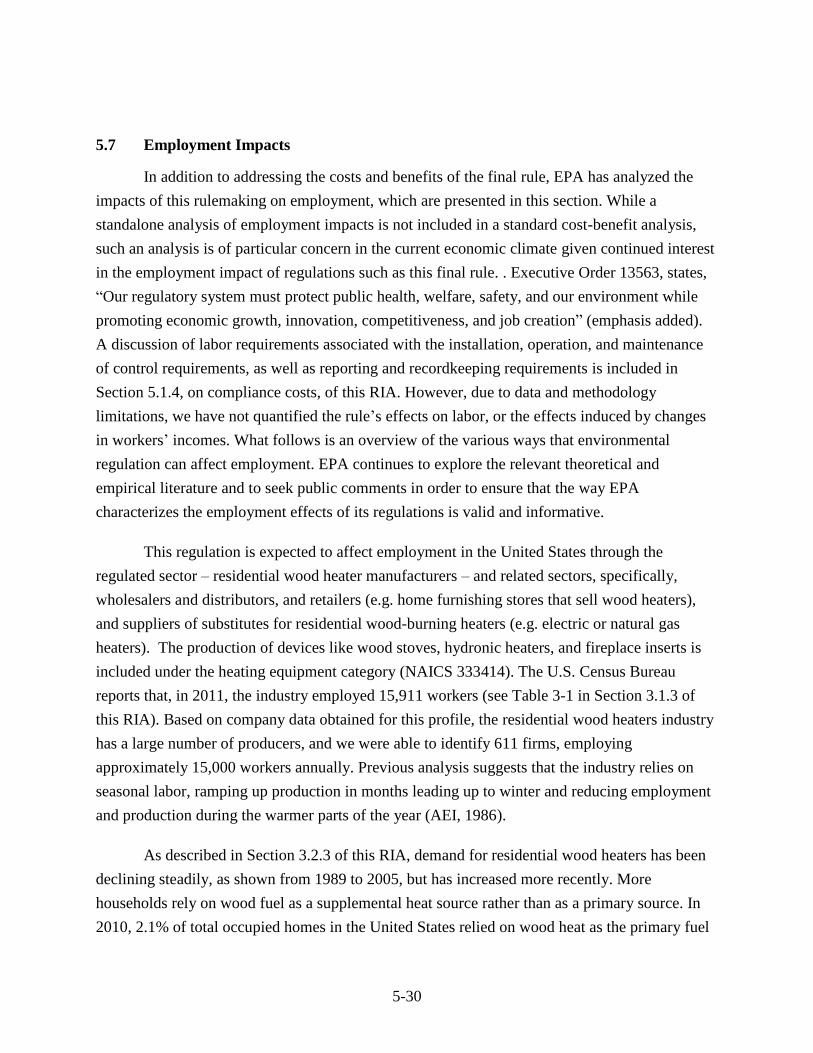
5-30
5.7 Employment Impacts
In addition to addressing the costs and benefits of the final rule, EPA has analyzed the
impacts of this rulemaking on employment, which are presented in this section. While a
standalone analysis of employment impacts is not included in a standard cost-benefit analysis,
such an analysis is of particular concern in the current economic climate given continued interest
in the employment impact of regulations such as this final rule. . Executive Order 13563, states,
“Our regulatory system must protect public health, welfare, safety, and our environment while
promoting economic growth, innovation, competitiveness, and job creation” (emphasis added).
A discussion of labor requirements associated with the installation, operation, and maintenance
of control requirements, as well as reporting and recordkeeping requirements is included in
Section 5.1.4, on compliance costs, of this RIA. However, due to data and methodology
limitations, we have not quantified the rule’s effects on labor, or the effects induced by changes
in workers’ incomes. What follows is an overview of the various ways that environmental
regulation can affect employment. EPA continues to explore the relevant theoretical and
empirical literature and to seek public comments in order to ensure that the way EPA
characterizes the employment effects of its regulations is valid and informative.
This regulation is expected to affect employment in the United States through the
regulated sector – residential wood heater manufacturers – and related sectors, specifically,
wholesalers and distributors, and retailers (e.g. home furnishing stores that sell wood heaters),
and suppliers of substitutes for residential wood-burning heaters (e.g. electric or natural gas
heaters). The production of devices like wood stoves, hydronic heaters, and fireplace inserts is
included under the heating equipment category (NAICS 333414). The U.S. Census Bureau
reports that, in 2011, the industry employed 15,911 workers (see Table 3-1 in Section 3.1.3 of
this RIA). Based on company data obtained for this profile, the residential wood heaters industry
has a large number of producers, and we were able to identify 611 firms, employing
approximately 15,000 workers annually. Previous analysis suggests that the industry relies on
seasonal labor, ramping up production in months leading up to winter and reducing employment
and production during the warmer parts of the year (AEI, 1986).
As described in Section 3.2.3 of this RIA, demand for residential wood heaters has been
declining steadily, as shown from 1989 to 2005, but has increased more recently. More
households rely on wood fuel as a supplemental heat source rather than as a primary source. In
2010, 2.1% of total occupied homes in the United States relied on wood heat as the primary fuel

5-31
source for home heating. About 10–12% of American households rely on wood when secondary
wood heat demand is counted, according to the U.S. Census Bureau and the Energy Information
Administration (EIA). Demand varies regionally, in part, due to availability of energy sources.
Current regional demand patterns are expected to continue, with the Northeast and Northwest
regions of the country driving wood fuel combustion demand, but analysts anticipate that the
wood heat product market will be embraced in other areas of the country in which wood and
biomass are viable and inexpensive fuel sources (Frost & Sullivan, 2010).
The extent to which an increase in the price of residential wood heaters due to this rule
would reduce the sales depends on the elasticity of demand for residential wood heaters.
However, as mentioned in Section 3 of this RIA, there are no recent empirical estimates of the
price elasticity of demand for residential wood heaters. An estimate of −1.6 was derived for use
in the RIA for the current Residential Wood Combustion NSPS (EPA, 1986). Information
provided by NERA in a public comment on the proposal included a price elasticity of demand of
-0.97 for hydronic heaters in ten states that regulate such devices (NERA, 2014a). Available
estimates for residential energy and heating fuel demand generally are relatively inelastic (i.e.,
there are only very small changes in demand in response to an increase in energy or fuel prices).
A recent RAND report suggests that in the short term, demand for electricity and natural gas in
residential markets is relatively inelastic (Bernstein and Griffin, 2005). There are a number of
close substitutes for residential wood heating devices that include electric and gas furnaces and
space heaters. The extent to which consumers are able to substitute between these options is
likely to vary depending on geographic location. Overall, the presence of good substitutes will
increase the elasticity of demand for wood heating equipment. In contrast, if locally-available
alternative heating fuels (e.g. electricity, fuel oil) are relatively higher-priced, it may make
switching away from wood heating equipment less likely and, ultimately, make demand for
wood heating equipment inelastic. Also, the elasticity may depend on whether the fuel in
question is a secondary source of fuel instead of a primary fuel source. Based on the available
information, including the RAND report, we do not expect sales of residential wood to fall
substantially due to this rule, particularly in the near-term.
From an economic perspective labor is an input into producing goods and services; if a
regulation requires that more labor be used to produce a given amount of output, that additional
labor is reflected in an increase in the cost of production. Moreover, when the economy is at full
employment, we would not expect an environmental regulation to have an impact on overall
employment because labor is being shifted from one sector to another. On the other hand, in
periods of high unemployment, employment effects (both positive and negative) are possible.

5-32
For example, an increase in labor demand due to regulation may result in a short-term net
increase in overall employment as workers are hired by the regulated sector to help meet new
requirements (e.g., to install new equipment) or by the environmental protection sector to
produce new abatement capital resulting in hiring previously unemployed workers . When
significant numbers of workers are unemployed, the opportunity costs associated with displacing
jobs in other sectors are likely to be smaller. And, in general, if a regulation imposes high costs
and does not increase the demand for labor, it may lead to a decrease in employment. The
responsiveness of industry labor demand depends on how these forces all interact. Economic
theory indicates that the responsiveness of industry labor demand depends on a number of
factors: price elasticity of demand for the product, substitutability of other factors of production,
elasticity of supply of other factors of production, and labor’s share of total production costs.
Berman and Bui (2001) put this theory in the context of environmental regulation, and suggest
that, for example, if all firms in the industry are faced with the same compliance costs of
regulation and product demand is inelastic, then industry output may not change much at all.
Regulations set in motion new orders for pollution control equipment and services. New
categories of employment have been created in the process of implementing environmental
regulations. When a regulation is promulgated, one typical response of industry is to order
pollution control equipment and services in order to comply with the regulation when it becomes
effective. On the other hand, the closure of plants that choose not to comply – and any changes
in production levels at plants choosing to comply and remain in operation - occur after the
compliance date, or earlier in anticipation of the compliance obligation. Environmental
regulation may increase revenue and employment in the environmental technology industry.
While these increases represent gains for that industry, they translate into costs to the regulated
industries required to install the equipment.
Environmental regulations support employment in many basic industries. Regulated firms
either hire workers to design and build pollution controls directly or purchase pollution control
devices from a third party for installation. Once the equipment is installed, regulated firms hire
workers to operate and maintain the pollution control equipment—much like they hire workers
to produce more output. In addition to the increase in employment in the environmental
protection industry (via increased orders for pollution control equipment), environmental
regulations also support employment in industries that provide intermediate goods to the
environmental protection industry. The equipment manufacturers, in turn, order steel, tanks,
vessels, blowers, pumps, and chemicals to manufacture and install the equipment. Currently in

5-33
most cases there is no scientifically defensible way to generate sufficiently reliable estimates of
the employment impacts in these intermediate goods sectors.
5.7.1 Employment Impacts within the Regulated Industry
It is sometimes claimed that new or more stringent environmental regulations raise
production costs thereby reducing production which in turn must lead to lower employment.
However, the peer-reviewed literature indicates that determining the direction of net employment
effects in a regulated industry is challenging due to competing effects. Environmental regulations
are assumed to raise production costs and thereby the cost of output, so we expect the “output”
effect of environmental regulation to be negative (higher prices lead to lower sales). On the other
hand, complying with the new or more stringent regulation requires additional inputs, including
labor, and may alter the relative proportions of labor and capital used by regulated firms in their
production processes. Two sets of researchers discussed here, Berman and Bui (2001) and
Morgenstern, Pizer, and Shih (2002),82 demonstrate using standard neoclassical microeconomics
that environmental regulations have an ambiguous effect on employment in the regulated
sector.59 These theoretical results imply that the effect of environmental regulation on
employment in the regulated sector is an empirical question and both sets of authors tested their
models empirically using different methodologies. Both Berman and Bui and Morgenstern et al.
examine the effect of environmental regulations on employment and both find that overall they
had no significant net impact on employment in the sectors they examined.
Berman and Bui (2001) developed an innovative approach to examine how an increase in
local air quality regulation that reduces nitrogen oxides (NOx) emissions affects manufacturing
employment in the South Coast Air Quality Management District (SCAQMD), which
incorporates Los Angeles and its suburbs. During the time frame of their study, 1979 to 1992, the
SCAQMD enacted some of the country’s most stringent air quality regulations. Using
SCAQMD’s local air quality regulations, Berman and Bui identify the effect of environmental
regulations on net employment in the regulated industries.83,84 The authors find that “while
regulations do impose large costs, they have a limited effect on employment” (Berman and Bui,
82 Berman, E. and L. T. M. Bui (2001). “Environmental Regulation and Labor Demand: Evidence from the South
Coast Air Basin.” Journal of Public Economics 79(2): 265-295. Morgenstern, R. D., W. A. Pizer, and J. S. Shih.
2002. Jobs versus the Environment: An Industry-Level Perspective.‖ Journal of Environmental Economics and
Management 43(3):412-436.
83 Note, like Morgenstern, Pizer, and Shih (2002), this study does not estimate the number of jobs created in the
environmental protection sector. 84 Berman and Bui include over 40 4-digit SIC industries in their sample.

5-34
2001, p. 269). Their conclusion is that local air quality regulation “probably increased labor
demand slightly” but that “the employment effects of both compliance and increased stringency
are fairly precisely estimated zeros [emphasis added], even when exit and dissuaded entry effects
are included” (Berman and Bui, 2001, p. 269).85
Morgenstern et al. (2002) estimated the effects of pollution abatement expenditures from
1979 to 1991 at the plant level on net employment in four highly regulated sectors (pulp and
paper, plastics, steel, and petroleum refining). Thus, in contrast to Berman and Bui (2001), this
study identifies employment effects by examining differences in abatement expenditures rather
than geographical differences in stringency. They conclude that increased abatement
expenditures generally have not caused a significant change in net employment in those sectors.
While the specific sectors Morgenstern et al. examined are different than the sectors considered
here, the methodology that Morgenstern et al. developed is still an informative way to
qualitatively, if not quantitatively,assess the effects of this rulemaking on employment in the
regulated sector.
While there is an extensive empirical, peer-reviewed literature analyzing the effect of
environmental regulations on various economic outcomes including productivity, investment,
competitiveness as well as environmental performance, there are only a few papers that examine
the impact of environmental regulation on employment, but this area of the literature has been
growing. As stated previously in this RIA section, empirical results from Berman and Bui (2001)
and Morgenstern et al (2002) suggest that new or more stringent environmental regulations do
not have a substantial impact on net employment (either negative or positive) in the regulated
sector. Nevertheless, other empirical research suggests that more highly regulated counties may
generate fewer jobs than less regulated ones (Greenstone 2002, Walker 2011). However, the
methodology used in these two studies cannot estimate whether aggregate employment is lower
or higher due to more stringent environmental regulation, it can only imply that relative
employment growth in some sectors differs between more and less regulated areas. List et al.
(2003) find some evidence that this type of geographic relocation, from more regulated areas to
less regulated areas may be occurring. Overall, the peer-reviewed literature does not contain
evidence that environmental regulation has a large impact on net employment (either negative or
positive) in the long run across the whole economy.
85 Including the employment effect of exiting plants and plants dissuaded from opening will increase the estimated
impact of regulation on employment.
5-35
While the theoretical framework laid out by Berman and Bui (2001) and Morgenstern et
al. (2002) still holds for the industries affected under this NSPS, important differences in the
markets and regulatory settings analyzed in their study and the setting presented here lead us to
conclude that it is inappropriate to utilize their quantitative estimates to estimate the employment
impacts from this proposed regulation. In particular, the industries used in these two studies as
well as the timeframe (late 1970’s to early 1990’s) are quite different than those in this proposed
rule. Furthermore, the control strategies analyzed for this RIA mostly include process and
design changes to reduce emissions during the production of affected heaters, and not after these
heaters are in operation.86 For instance, use of a catalyst combustor is common in wood stoves in
order to reduce emissions and also improve heat efficiency. Retrofits are highly uncommon
because replacing the wood stove is often a more economical alternative. On the other hand, the
pollution control strategies examined by Berman and Bui and Morgenstern et al. are primarily
add-on or end-of-line pollution controls. For these reasons we conclude there are too many
uncertainties as to the transferability of the quantitative estimates in these two studies to apply
their estimates to quantify the employment impacts within the regulated sectors for this
regulation, though these studies have usefulness for qualitative assessment of employment
impacts.
The preceding sections have outlined the challenges associated with estimating net
employment effects in the regulated sector and in the environmental protection sector and labor
supply impacts. These challenges make it very difficult to accurately produce net employment
estimates for the whole economy that would appropriately capture the way in which costs,
compliance spending, and environmental benefits propagate through the macro-economy.
Quantitative estimates are further complicated by the fact that macroeconomic models often have
very little sectoral detail and usually assume that the economy is at full employment. EPA’s
Science Advisory Board (SAB) is currently in the process of seeking input from an independent
expert panel on modeling economy-wide impacts, including employment effects.
5.7.2. Conclusion
Economic theory predicts that the total effect of an environmental regulation on labor
demand in regulated sectors is not necessarily positive or negative. Peer-reviewed econometric
studies that use a structural approach, applicable to in the regulated sectors, converge on the
finding that such effects, whether positive or negative, have been small.
86 More detail on how emission reductions expected from compliance with this rule can be obtained can be found in
Section 4 of this RIA.

5-36
References for Employment Impacts Analysis
Greenstone, M. (2002). “The Impacts of Environmental Regulations on Industrial Activity: Evidence
from the 1970 and 1977 Clean Air Act Amendments and the Census of Manufactures.” Journal of
Political Economy 110(6): 1175-1219.
List, J. A., D. L. Millimet, P. G. Fredriksson, and W. W. McHone (2003). “Effects of Environmental
Regulations on Manufacturing Plant Births: Evidence from a Propensity Score Matching Estimator.” The
Review of Economics and Statistics 85(4): 944-952.
Walker, Reed. (2011).“Environmental Regulation and Labor Reallocation." American Economic
Review: Papers and Proceedings, 101(2).
6-1
SECTION 6
SMALL ENTITY SCREENING ANALYSIS
The Regulatory Flexibility Act as amended by the Small Business Regulatory
Enforcement Fairness Act (SBREFA) generally requires an agency to prepare a regulatory
flexibility analysis of any rule subject to notice and comment rulemaking requirements under the
Administrative Procedure Act or any other statute, unless the agency certifies that the rule will
not have a significant economic impact on a substantial number of small entities. Small entities
include small businesses, small governmental jurisdictions, and small not-for-profit enterprises.
After considering the economic impact of the rule on small entities, the screening
analysis indicates that we cannot conclude that this rule may not have a significant economic
impact on a substantial number of small entities (or “SISNOSE”) for certain residential wood
heating products covered under the revised NSPS. For this analysis EPA considered sales and
revenue tests for establishments owned by representative small entities that manufacture or
construct residential wood heating devices.
6.1 Small Entity Data Set
The industry sectors covered by the rule were identified during the development of the
cost analysis (see Sections 3 and 5). The Statistics of U.S. Businesses (SUSB) provides national
information on the distribution of economic variables by industry and enterprise size (U.S.
Census, 2008a, 2008b). The Census Bureau and the Office of Advocacy of the Small Business
Administration (SBA) supported and developed these files for use in a broad range of economic
analyses.87 Statistics include the total number of establishments and receipts for all entities in an
industry; however, many of these entities may not necessarily be covered by the final rule. SUSB
also provides statistics by enterprise employment and receipt size.
The Census Bureau’s definitions used in the SUSB are as follows:
Establishment: An establishment is a single physical location where business is
conducted or where services or industrial operations are performed.
Receipts: Receipts (net of taxes) are defined as the revenue for goods produced,
distributed, or services provided, including revenue earned from premiums,
commissions and fees, rents, interest, dividends, and royalties. Receipts exclude all
revenue collected for local, state, and federal taxes.
87 See http://www.census.gov/csd/susb/ and http://www.sba.gov/advo/research/data.html for additional details.

6-2
Enterprise: An enterprise is a business organization consisting of one or more
domestic establishments that were specified under common ownership or control. The
enterprise and the establishment are the same for single-establishment firms. Each
multi-establishment company forms one enterprise—the enterprise employment and
annual payroll are summed from the associated establishments. Enterprise size
designations are determined by the summed employment of all associated
establishments.
Because the SBA’s business size definitions (SBA, 2014) apply to an establishment’s
“ultimate parent company,” we assumed in this analysis that the “enterprise” definition above is
consistent with the concept of ultimate parent company that is typically used for SBREFA
screening analyses and the terms are used interchangeably.
6.2 Small Entity Economic Impact Measures
The analysis generated a set of establishment sales tests (represented as cost-to-receipt
ratios) for NAICS codes associated with sectors listed in Table 6-1. It should be noted that the
cost-to-receipt ratios presented in Table 5-5 of this RIA are estimated at the product level and are
not calculated to inform the small entity analysis, while the small entity impact estimates will be
estimated at the establishment (place of business) level. Although the appropriate SBA size
definition should be applied at the parent company (enterprise) level, we can only compute and
compare ratios for a model establishment owned by an enterprise within an SUSB size range
(employment or receipts). Using the SUSB size range helps us account for receipt differences
between establishments owned by large and small enterprises and also allows us to consider the
variation in small business definitions across affected industries. Using establishment receipts is
also a somewhat conservative approach, because an establishment’s parent company (the
“enterprise”) may have other economic resources that could be used to cover the costs of the
final rule. It should be noted that these impacts are for the 2015–2020 time frame; as mentioned
earlier in this RIA, the annualized costs considered in this analysis reflect an average of the
rule’s compliance costs incurred by affected sources each year from promulgation through 2020.
6.2.1 Establishment Employment and Receipts
The sales test compares a representative establishment’s total annual compliance costs to
the average establishment receipts for enterprises in several size categories.88 For industries with
SBA employment size standards, we calculated average establishment receipts for each
enterprise employment range (Table 6-2). For industries with SBA receipt size standards, we
calculated average establishment receipts for each enterprise receipt range (Table 6-3). The
88 For the 1 to 20 employee category, we excluded SUSB data for enterprises with zero employees. These
enterprises did not operate the entire year.

6-3
analysis assumes that the majority of affected entities are covered under hardware manufacturing
(NAICS 332510) and heating equipment manufacturing (NAICS 333414). We use establishment
data from the 2007 Economic Census because that data is the most recent release of public
establishment-level information for the industries impacted by this proposal.
Table 6-1. Revised NSPS for Residential Wood Heating Devices: Affected Sectors and
SBA Small Business Size Standards
Industry Description
Corresponding
NAICS
SBA Size Standard for Businesses
(July 14, 2014)
Type of Small
Entity
Hardware manufacturing 332510 500 employees All product
types
Heating equipment (except warm air)
manufacturing
333414 500 employees All product
types
Plumbing and heating equipment and
supplies (hydronics) merchant
wholesalers
423720 100 employees All product
types
All other home furnishing stores 442299 $20.5 million
in annual receipts
Business
However, the revised NSPS has the potential to affect small entities classified as new
home construction. In addition, wholesalers of imported residential heating devices may also be
affected if these establishments are required to certify imported products.
6.2.2 Establishment Compliance Cost
Annual entity compliance costs vary depending on the product type manufactured and the
number of product models they would need to redesign under the revised NSPS as mentioned in
Section 5 of this RIA. For this analysis compliance costs were estimated based on the average
development costs defined in the engineering cost analysis, presented in Section 5-1. The
analysis assumes that manufacturers have between two and seven model fireboxes that would be
subject to the new NSPS. There is limited information on the actual number of model fireboxes
associated with small businesses. Hence, for purposes of the small entity screening analysis, we
assumed that smaller companies maintain fewer than three firebox models that would be subject
to the revised NSPS. In the absence of better data, EPA believes that between one and three
firebox models is a reasonable assumption for our analysis of impacts to potentially affected
small businesses.

6-4
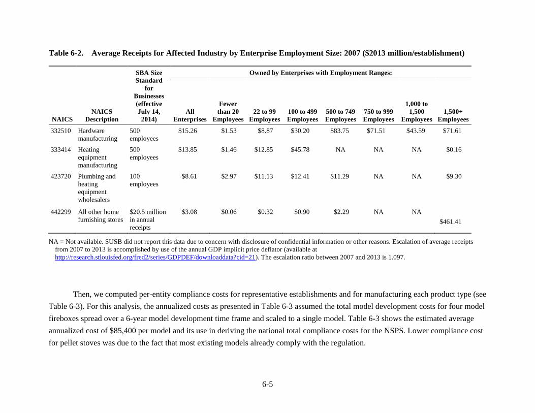
6-5
Table 6-2. Average Receipts for Affected Industry by Enterprise Employment Size: 2007 ($2013 million/establishment)
SBA Size
Standard
for
Businesses
(effective
July 14,
2014)
Owned by Enterprises with Employment Ranges:
NAICS
NAICS
Description
All
Enterprises
Fewer
than 20
Employees
22 to 99
Employees
100 to 499
Employees
500 to 749
Employees
750 to 999
Employees
1,000 to
1,500
Employees
1,500+
Employees
332510 Hardware
manufacturing
500
employees
$15.26 $1.53 $8.87 $30.20 $83.75 $71.51 $43.59 $71.61
333414 Heating
equipment
manufacturing
500
employees
$13.85 $1.46 $12.85 $45.78 NA NA NA $0.16
423720 Plumbing and
heating
equipment
wholesalers
100
employees
$8.61 $2.97 $11.13 $12.41 $11.29 NA NA $9.30
442299 All other home
furnishing stores
$20.5 million
in annual
receipts
$3.08 $0.06 $0.32 $0.90 $2.29 NA NA
$461.41
NA = Not available. SUSB did not report this data due to concern with disclosure of confidential information or other reasons. Escalation of average receipts
from 2007 to 2013 is accomplished by use of the annual GDP implicit price deflator (available at
http://research.stlouisfed.org/fred2/series/GDPDEF/downloaddata?cid=21). The escalation ratio between 2007 and 2013 is 1.097.
Then, we computed per-entity compliance costs for representative establishments and for manufacturing each product type (see
Table 6-3). For this analysis, the annualized costs as presented in Table 6-3 assumed the total model development costs for four model
fireboxes spread over a 6-year model development time frame and scaled to a single model. Table 6-3 shows the estimated average
annualized cost of $85,400 per model and its use in deriving the national total compliance costs for the NSPS. Lower compliance cost
for pellet stoves was due to the fact that most existing models already comply with the regulation.

6-6
Table 6-3. Per-Entity Annualized Compliance Costs by Product Type— with NSPS ($2013 millions)
Product Type
No.
Establishments
Assumed Affected
Models per
Establishmenta
Annual
Compliance
Cost per Model
Firebox
($ millions)
Total Industry Costs—
NSPS
($ millions)
Wood stoves 42 3 $0.02 $3.02
Single burn rate stoves 3 7 $0.04 $0.87
Pellet stoves 31 4 $0.01 $1.52
Forced-air furnaces 7 7 $0.31 $15.36
Hydronic heating systems 30 4 $0.21 $24.88
National Annualized
Compliance Cost
$45.7
a Table totals may differ because of rounding. Number of models is based on estimates in the Unit Cost memo, EC/R, January 30, 2015.
For each case in this analysis, the number of models each representative establishment must redesign to comply with the NSPS
emission limits analyzed in this RIA varies by product type. The total annualized compliance cost per establishment
(TAC/establishment) is calculated by multiplying the number of firebox models requiring redesign by the average annualized cost per
model across product types and weighting by the number of models for each product type. Thus, product types with a larger number
of affected establishments and assumed models per establishment will have a larger effect on the estimate of TAC/establishment when
not considering the costs for product types. This information is summarized above in Table 6-3 and is provided in more detail in the
unit cost memo. The greater the number of models, the greater the effect on the total annualized compliance cost. Using this
approach, the TAC/establishment is $103,700. Table 6-3 presents the assumed number of models per establishment by product type.

6-7
Table 6-4. Representative Establishment Costs Used for Small Entity Analysis ($2013)
Best Estimate
Number of models requiring redesign 2
Annual cost per model $103,700
Average annual cost per establishment $207,400
For the sales test, we divided the representative establishment compliance costs reported in Table 6-4 by the representative
establishment receipts reported in Tables 6-2 and 6-3. This is known as the cost-to-receipt (i.e., sales) ratio, or the “sales test.” The
“sales test” is the impact methodology EPA employs in analyzing small entity impacts as opposed to a “profits test,” in which
annualized compliance costs are calculated as a share of profits.
Information on annual revenues or sales is more commonly available data for entities normally affected by EPA regulations,
and profits data normally made available are often not the true profit earned by firms because of accounting and tax considerations.
Revenues as typically published are usually correct figures and are more reliably reported when compared with profit data. The use of
a “sales test” for estimating small business impacts for a rulemaking such as this
6-8
one is consistent with guidance offered by EPA on compliance with SBREFA89 and is consistent with guidance published by the
SBA’s Office of Advocacy that suggests that cost as a percentage of total revenues is a metric for evaluating cost increases on small
entities in relation to increases on large entities (SBA, 2003).90 The annualized cost per sales for a company represents the maximum
price increase in affected product needed for the company to completely recover the annualized costs imposed by the regulation.
For purposes of this analysis, EPA assumes most small entities in the residential wood heating industry are likely to
manufacture fewer than three distinctive firebox models and in many cases they would support only one model. We assume for this
analysis that most small entities in this industry will manufacture an average of two distinctive firebox models. Hence, EPA believes
that the estimate in Table 6-4 above is the most representative establishment costs to assess impacts on small businesses. If the cost-to-
receipt ratio is less than 1%, then we consider the rule to not have a significant impact on the establishment (and, company) in
question. Table 6-5 presents the cost-to-receipt ratios for each category of establishments (establishments with ratios that exceed 1%
under each case are highlighted) for the final NSPS.
89 The SBREFA compliance guidance to EPA rule writers (EPA, 2006a) regarding the types of small business analysis that should be considered can be found at
http://www.epa.gov/sbrefa/documents/rfaguidance11-00-06.pdf, pp. 24-25. 90 This compliance guide produced by SBA can be found at http://www.sba.gov/sites/default/files/rfaguide_0512_0.pdf.
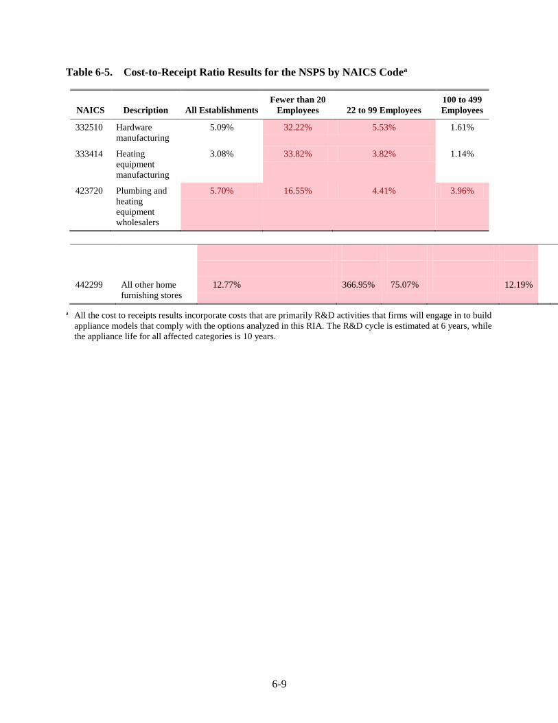
6-9
Table 6-5. Cost-to-Receipt Ratio Results for the NSPS by NAICS Codea
NAICS Description All Establishments
Fewer than 20
Employees 22 to 99 Employees
100 to 499
Employees
332510 Hardware
manufacturing
5.09% 32.22% 5.53% 1.61%
333414 Heating
equipment
manufacturing
3.08% 33.82% 3.82% 1.14%
423720 Plumbing and
heating
equipment
wholesalers
5.70% 16.55% 4.41% 3.96%
442299 All other home
furnishing stores
12.77% 366.95% 75.07% 12.19%
a All the cost to receipts results incorporate costs that are primarily R&D activities that firms will engage in to build
appliance models that comply with the options analyzed in this RIA. The R&D cycle is estimated at 6 years, while
the appliance life for all affected categories is 10 years.

6-10
6.3 Analysis Results
In our small entity analysis for the final rule, using an annual compliance cost of
$207,800 as the estimated cost borne by an affected small entity, establishments in NAICS
332510, 333414, and 423720 with fewer than 500 employees have cost-to-receipt ratios higher
than 1% as shown in Table 6-5. Establishments in NAICS 442299 with receipts less than $10
million have cost-to-receipt ratios considerably higher than 1%.
After considering the economic impacts of this rule on small entities, we cannot certify
that this action will not have a significant economic impact on a substantial number of small
entities. This certification is based on the economic impact of this action to all affected small
entities across all industries affected. Using the estimate of impacts presented earlier in this
chapter, we estimate that all small entities will have annualized costs of greater than 1% of their
sales in all industries with establishments of fewer than 100 employees and NAICS 236115,
238140, and 442299 with receipts less than $20 million. Those establishments in NAICS
332510, 333414, and 423720 with cost-to-receipt ratios higher than 1% account for more than
85% of small entities. Establishments in NAICS 442299 with cost-to-receipt ratios higher than
1% account for more than 99% of small entities. We thus conclude that we cannot certify that
there is not a significant economic impact on a substantial number of small entities (SISNOSE)
for this rule.
It should be noted that the cost to receipts analysis included in this RIA reflect the large
majority of annualized costs that are composed of research and development (R&D) activities
(nearly 90%, based on the manufacturers’ cost memorandum) that have a shorter life than the
total life of affected appliances—six years for an R&D cycle as mentioned in section 5 of this
RIA compared to 10 years for the life of affected appliances. The impacts on small entities
should be understood in the context that a large share of the estimated annualized costs reflect
expenses in the early years of the appliance life, and only a small share recurs each year over the
entire appliance life of 10 years. In addition, the application of these costs for the options
analyzed in this RIA will lead to a somewhat conservative (or, over-stated) cost estimate as
stated previously in section 5.1.3. One example of this is that all hydronic heaters will undergo
R&D beginning in 2015 to comply with the final NSPS; there is a small percentage of hydronic
heaters that already meet the emission limits under each option as mentioned in Section 4 in the
RIA. Similar assumptions are also made in the cost estimates for single burn rate stoves and

6-11
forced air furnaces. Given these two considerations, the costs that are included in the cost to sales
analyses presented in this RIA could be somewhat overstated in nature, and the cost to receipts
impacts shown above should be understood in that context.
A sensitivity analysis showing the effect of the R&D cycle lifespan on the cost to sales
estimates for each option is below. Table 6-6 shows how the model firebox costs that are input
to the cost to sales (and small business) analyses will change with changes to the R&D cycle
lifespan.
Table 6-6. Total Annual Cost (TAC) per Appliance Model Firebox– for Varying
Annualized R&D Cycle Lifespans
Annualized R&D
Cycle Lifespan
(Years)
TAC/Appliance Model Firebox
(2013$)
TAC per Establishment
4 $146,000 292,000
6* 103,700 $ 207,400
10 70,540 141,080
20 46,760 93,520
*As mentioned in Section 5 of this RIA, six years represents the annualized R&D cycle lifespan
incorporated in the cost estimates for the RWH NSPS rule. In addition, each affected firm or establishment
is estimated to have two affected models on average. The interest rate for estimating TAC per appliance
model firebox in this table is 7%.
The total annual cost per appliance model is the value of costs included in the cost to
sales estimates to calculate these values. Each small entity is expected to modify 2 appliance
models on average in order to comply with the rule, an assumption we established earlier in this
section of the RIA. We assume each small entity owns only one establishment (or place of
business). Hence, the total annual cost to each small entity is twice the annual cost per appliance
model. The annual cost to sales in the RIA will change proportionately to a change in the TAC
since the sales estimates are presumed to remain constant for purposes of this analysis.
As shown in Table 6-6, with an increase in the R&D cycle lifespan from 6 to 10 years,
the TAC/appliance model estimate falls to $70,540 from $103,700. The new TAC/appliance
model estimate is 32% less than before. Thus, the cost to sales estimates will fall by 32% from
the previous values. If the R&D cycle lifespan increases from 6 to 20 years, the TAC/appliance
model estimate falls to $46,760 from $103,700. Thus, the cost to sales estimate will fall by 55%
from the previous values. Finally, if the R&D cycle lifespan is reduced to 4 years, the
TAC/appliance model estimate increases to $146,000 from $103,700. The new TAC/appliance

6-12
model estimate is now 41% higher than before. Thus, the cost to sales estimates will increase by
41% from the values that use an R&D cycle lifespan of 6 years.
Table 6-7 contains estimates of the changes in the cost to sales estimates for the NSPS
with an increase in the R&D cycle lifespan to 10 and 20 years from 6 years. The estimates with
the change in R&D cycle lifespan to 10 and 20 years are in parentheses; the other values are
those for the NSPS.
Table 6-7. Cost-to-Sales Ratio Sensitivity Analysis Results Reflecting Different
R&D Cycle Lifespans for the NSPS by NAICS Code*
NAICS Industry
Description
All
Establishments
Establishments
with Fewer than
20 Employees (%)
Establishments
with Between 20
and 99
Employees (%)
Establishments
with Between
100 and 499
Employees (%)
332510 Hardware
manufacturing
5.90 (3.47, 2.30) 32.22 (21.90,
14.48)
5.54 (3.77, 2.49) 1.61 (1.09, 0.72)
333414 Heating
equipment
manufacturing
3.08 (2.08, 1.37) 33.82(23.03, 15.22) 3.81(2.59, 1.71) 1.14 (0.77, 0.51)
423720 Plumbing and
heating
equipment
wholesalers
5.70 (3.87, 2.55) 16.54 (11.24, 7.43) 4.44(3.00, 1.98) 3.97 (2.69, 1.78)
* The first value in parentheses is the cost to sales estimate for a 10 year R&D cycle lifespan; the
second value is the cost to sales estimates for a 20 year R&D cycle lifespan. The values that are not in
the parentheses are the cost to sales estimates for a 6 year R&D cycle lifespan, the value used in the
estimates of costs for the NSPS.
6.4 Final Regulatory Flexibility Analysis (FRFA)
An FRFA illustrates how EPA considers the rule’s small entity effects for a final rule and
provides information about how the objectives of the rule were achieved while minimizing
significant economic impacts on small entities. We provide a summary of FRFA elements; the
preamble to this final rule provides additional details.
6.4.1 Reasons Why Action Is Being Considered
This rule was developed following a Clean Air Act (CAA) section 111(b)(1)(B) periodic
review of the existing residential wood heater new source performance standards (NSPS) and
because emissions from residential wood heaters can be a significant source of air pollution, and
thus adverse health effects, in some areas.
6-13
6.4.2 Statement of Objectives and Legal Basis of Proposed Rule
The EPA is amending Standards of Performance for New Residential Wood Heaters, and
is adding one new subpart: Standards of Performance for New Residential Hydronic Heaters and
Forced-Air Furnaces. This final rule achieves several objectives, including applying updated
emission limits that reflect BSER; improving coverage of the broad suite of residential wood
heaters; improving the test methods; and streamlining the certification process. This final rule
does not include any requirements on heaters solely fired by coal, gas or oil. This final rule does
not establish new emissions limits for existing heaters. This rule was developed under the
authority of CAA section 111.
6.4.3 Response to Any Comments to the Proposed Rule Filed by the Chief Counsel for
Advocacy of the SBA
The SBA’s Chief Counsel for Advocacy did not file any comments in response to the
proposed rule.
6.4.4 Description and Estimate of the Number of Small Entities
Small entities that EPA anticipates being affected by the standards would include almost
all manufacturers of wood heaters listed earlier this document. EPA estimates that roughly 250–
300 U.S. companies manufacture residential wood heaters. EPA believes that approximately
90% of these manufacturers meet the SBA small-entity definition of having fewer than 500
employees.
6.4.5 Description of Impact Methodology and Compliance Costs
A discussion of the methodology used to estimate cost impacts is presented in Section 5
of this RIA.
6.4.5 Panel Recommendations for Small Business Flexibilities
As required by section 609(b) of the RFA, as amended by the Small Business Regulatory
Enforcement Fairness Act (SBREFA), the EPA also convened a Small Business Advocacy
Review Panel (Panel) to obtain advice and recommendations of representatives of the small
entities that potentially would be subject to the rule's requirements. The following paragraphs
describe the process, the type of small entity representatives, the outreach efforts and the Panel
members.
6-14
Well before beginning the formal SBREFA process, the EPA actively engaged in
outreach with HPBA, MHA and PFI and many of their member companies to discuss the rule
under development and to provide these contacts with an early opportunity to ask questions and
discuss their concerns.91 The EPA provided each small business with general information on the
SBREFA process and background information on the NSPS rulemaking process and current
schedule.
Based on consultations with the Small Business Administration, and resulting from
solicited self-nominations, we prepared a list of 30 potential Small Entity Representatives
(SERs), from residential wood heating appliance manufacturers (wood heaters, pellet
heaters/stoves, hydronic heaters, forced-air furnaces and masonry heaters), other wood-burning
appliance manufacturers (fireplaces, cook stoves), equipment suppliers, chimney sweeps, test
laboratories, masons and trade associations. Once the official pre-Panel process began and
potential SERs were identified, the EPA held an outreach meeting with the potential SERs and
invited representatives from the Office of Advocacy of the Small Business Administration
(OA/SBA) and the Office of Information and Regulatory Affairs within the Office of
Management and Budget (OIRA/OMB) on June 29, 2010, to solicit their feedback on the
upcoming proposed rulemaking. Representatives from 26 of the 30 companies and organizations
that we selected as potential SERs for this SBREFA process participated in the meeting (in
person and by phone). At that meeting, the EPA solicited written comments from the potential
SERs, which were later summarized and shared with the Panel as part of the convening
document.
The SBAR Panel convened on August 4, 2010. The Panel consisted of representatives of
the EPA, OA/SBA and OIRA/OMB. The Panel held a formal outreach meeting/teleconference
with the SERs on August 25, 2010. To help the SERs prepare for this meeting, on August 11,
2010, the Panel sent a list of questions, preliminary cost information and other materials to each
of the SERs via email. Additional materials were emailed to the SERs on August 19, 2010. The
Panel provided the opportunity for questions and comment during the meeting on various aspects
of the proposal being developed, including the expanded scope of the rule, changes to the current
requirements under consideration, preliminary cost information and follow up from the June 29,
2010, meeting on the SERs’ ideas for regulatory flexibility. During the August 25 meeting, SERs
voiced general support for the planned proposed rule and shared specific concerns with the Panel
91 Also, as noted in the proposal preamble in the discussion of development of the proposed hydronic heater
emission limits, the EPA worked with the hydronic heater industry in 2006 to develop a voluntary partnership
program to encourage manufacture of cleaner models, www.epa.gov/burnwise/participation.

6-15
members. As a result of this meeting, the EPA received many useful verbal comments, and the
EPA received many helpful written comments by September 10, 2010.
Consistent with the RFA/SBREFA requirements, the Panel evaluated the assembled
materials and small-entity comments on issues related to elements of the Interim Regulatory
Flexibility Analysis. A copy of the Panel final full report is included in the docket for this rule.
We have attempted to follow the Panel’s recommendations to the degree we can while also
ensuring that the options are practicable, enforceable, environmentally sound and consistent with
the CAA. For those recommendations not adopted by the EPA, we included an explanation at
proposal for why we rejected them.
In addition, the EPA is preparing a Small Entity Compliance Guide to help small entities
comply with this rule. Small entities can obtain of a copy of this guide at
http://www.epa.gov/rfa/compliance-guides.html or http://www2.epa.gov/residential-wood-
heaters. We expect the Small Entity Compliance Guide to be available by April 2015.

7-1
SECTION 7
HUMAN HEALTH BENEFITS OF EMISSIONS REDUCTIONS
7.1 Synopsis
Implementation of emissions limits required by the residential wood heaters NSPS is
expected to reduce direct emissions of PM2.5. These reductions result from the imposition of
tightened and new PM emissions limits for a number of emissions categories as described in
Section 2 of this RIA. In this section, we quantify the monetized benefits for this rule associated
with reduced exposure to ambient fine particulate matter (PM2.5) resulting from the reduction of
direct emissions of PM2.5. The total PM2.5 reductions are the consequence of the expected design
changes to the affected appliances needed in order to meet the emissions limits analyzed in this
RIA. We estimate the total monetized benefits for the NSPS to be $3.4 billion to $7.6 billion at a
3% discount rate and $3.1 billion to $6.9 billion at a 7% discount rate on a yearly average
between 2015 and 2020. All estimates are in 2013$ as they are summarized in Table 7-2. These
estimates reflect the monetized human health benefits of reducing cases of morbidity and
premature mortality among populations exposed to PM2.5 reduced by this rule.
Data, resources, and methodological limitations prevented EPA from monetizing the
benefits from several important benefit categories. Included among the nonmonetized benefits
are those associated with reduced exposure to about 9,300 tons of VOCs. VOCs are also
precursors to ozone formation and therefore reducing health impact due to ozone exposure.
Further, this rule would reduce each year 46,100 tons of CO, black carbon emissions, and several
HAP emissions such as benzene, formaldehyde, and dioxin. This rule will also reduce ecosystem
effects, and visibility impairment due to PM emissions.
7.2 PM2.5-Related Human Health Benefits
This rule is expected to reduce direct emissions of PM and emissions of VOCs, which are
precursors to formation of ambient PM2.5. Therefore, reducing these emissions would also reduce
human exposure to ambient PM2.5 and the incidence of PM2.5-related health effects. In this
section, we provide an overview of the PM2.5-related benefits. A full description of the
underlying data, studies, and assumptions is provided in the PM NAAQS RIA (U.S. EPA,
2012a).
In implementing this rule, emission controls may lead to reductions in ambient PM2.5
concentrations below the National Ambient Air Quality Standards (NAAQS) for PM in some
areas and assist other areas with attaining the PM NAAQS. Because the PM NAAQS RIA (U.S.
7-2
EPA, 2012a) also calculated PM benefits, there are important differences worth noting in the
design and analytical objectives of each RIA. The NAAQS RIAs illustrate the potential costs and
benefits of attaining a revised air quality standard nationwide based on an array of emission
reduction strategies for different sources including known and unknown controls, incremental to
implementation of existing regulations and controls needed to attain the current standards. In
short, NAAQS RIAs hypothesize, but do not predict, the reduction strategies that States may
choose to enact when implementing a revised NAAQS. The setting of a NAAQS does not
directly result in costs or benefits, and as such, the NAAQS RIAs are merely illustrative and the
estimated costs and benefits are not intended to be added to the costs and benefits of other
regulations that result in specific costs of control and emission reductions. However, it is
possible that some costs and benefits associated with the required emission controls estimated in
this RIA may account for the same air quality improvements as estimated in the illustrative PM
NAAQS RIA.
By contrast, the emission reductions for implementation rules such as this rulemaking are
generally for specific, well-characterized sources. In general, EPA is more confident in the
magnitude and location of the emission reductions for implementation rules. As such, emission
reductions achieved under these and other promulgated implementation rules will ultimately be
reflected in the baseline of future NAAQS analyses, which would reduce the incremental costs
and benefits associated with attaining revised future NAAQS. EPA remains forward looking
towards the next iteration of the 5-year review cycle for the NAAQS. As a result, EPA does not
re-issue NAAQS RIAs that retroactively update the baseline to account for implementation rules
promulgated after a NAAQS RIA outside of the NAAQS review process. For more information
on the relationship between the NAAQS and rules that are not ambient standards, such as
analyzed here, please see Section 1.3 of the PM NAAQS RIA (U.S. EPA, 2012a).
7.2.1 Health Impact Assessment
The Integrated Science Assessment for Particulate Matter (PM ISA) (U.S. EPA, 2009)
identified the human health effects associated with ambient PM2.5, which include premature
mortality and a variety of morbidity effects associated with acute and chronic exposures. Table
7-1 provides the quantified and unquantified benefits captured in EPA’s benefits estimates for
reduced exposure to ambient PM2.5. Although the table below does not include entries for the
unquantified health effects such as exposure to ozone and NO2 nor welfare effects such as
ecosystem effects and visibility impairment, these effects are itemized in Chapters 5 and 6 of the

7-3
Table 7-1. Human Health Effects of Ambient PM2.5
Category Specific Effect
Effect Has
Been
Quantified
Effect Has
Been
Monetized
More
Information
in PM
NAAQS RIA
Improved Human Health
Reduced incidence of
premature mortality
from exposure to
PM2.5
Adult premature mortality based on cohort
study estimates and expert elicitation
estimates (age >25 or age >30)
Section 5.6
Infant mortality (age <1) Section 5.6
Reduced incidence of
morbidity from
exposure to PM2.5
Non-fatal heart attacks (age > 18) Section 5.6
Hospital admissions—respiratory (all
ages)
Section 5.6
Hospital admissions—cardiovascular (age
>20)
Section 5.6
Emergency room visits for asthma (all
ages)
Section 5.6
Acute bronchitis (age 8–12) Section 5.6
Lower respiratory symptoms (age 7–14) Section 5.6
Upper respiratory symptoms (asthmatics
age 9–11)
Section 5.6
Asthma exacerbation (asthmatics age 6–
18)
Section 5.6
Lost work days (age 18–65) Section 5.6
Minor restricted-activity days (age 18–65) Section 5.6
Chronic Bronchitis (age >26) —a —a Section 5.6
Emergency room visits for cardiovascular
effects (all ages)
—a —a Section 5.6
Strokes and cerebrovascular disease (age
50–79)
—a —a Section 5.6
Other cardiovascular effects (e.g., other
ages)
— — PM ISAb
Other respiratory effects (e.g., pulmonary
function, non-asthma ER visits, non-
bronchitis chronic diseases, other ages and
populations)
— — PM ISAb
Reproductive and developmental effects
(e.g., low birth weight, pre-term births,
etc.)
— — PM ISAb,c
Cancer, mutagenicity, and genotoxicity
effects
— — PM ISAb,c
a We assess these benefits qualitatively due to time and resource limitations for this analysis. In the PM NAAQS
RIA, these benefits were quantified in a sensitivity analysis, but not in the core analysis. b We assess these benefits qualitatively because we do not have sufficient confidence in available data or methods.

7-4
c We assess these benefits qualitatively because current evidence is only suggestive of causality or there are other
significant concerns over the strength of the association.
PM NAAQS RIA (U.S. EPA, 2012a). It is important to emphasize that the list of unquantified
benefit categories is not exhaustive, nor is quantification of each effect complete.
We follow a “damage-function” approach in calculating benefits, which estimates
changes in individual health endpoints (specific effects that can be associated with changes in air
quality) and assigns values to those changes assuming independence of the values for those
individual endpoints. Because EPA rarely has the time or resources to perform new research to
measure directly either the health outcomes or their values for regulatory analyses, our estimates
are based on the best available methods of benefits transfer, which is the science and art of
adapting primary research from similar contexts to estimate benefits for the environmental
quality change under analysis.
The health impact assessment (HIA) quantifies the changes in the incidence of adverse
health impacts resulting from changes in human exposure to PM2.5 or other air pollutants. We use
the environmental Benefits Mapping and Analysis Program (BenMAP) to systematize health
impact analyses by applying a database of key input parameters, including population
projections, health impact functions, and valuation functions (Abt Associates, 2012). For this
assessment, the HIA is limited to those health effects that are directly linked to ambient PM2.5
concentrations. Epidemiological studies generally provide estimates of the relative risks of a
particular health effect for a given increment of air pollution (often per 10 µg/m3 for PM2.5).
These relative risks can be used to develop risk coefficients that relate a unit reduction in PM2.5
to changes in the incidence of a health effect. We refer the reader to section 5.6 of the PM
NAAQS RIA for more information regarding the epidemiology studies and risk coefficients
applied in this analysis (U.S. EPA, 2012a), and we briefly elaborate on adult premature mortality
below. The size of the mortality effect estimates from epidemiological studies, the serious nature
of the effect itself, and the high monetary value ascribed to prolonging life make mortality risk
reduction the most significant health endpoint quantified in this analysis.
Considering a substantial body of published scientific literature, reflecting thousands of
epidemiology, toxicology, and clinical studies, the PM ISA documents the association between
elevated PM2.5 concentrations and adverse health effects, including increased premature
mortality (U.S. EPA, 2009). The PM ISA, which was twice reviewed by the Clean Air Scientific
Advisory Committee of EPA’s Science Advisory Board (SAB-CASAC) (U.S. EPA-SAB, 2009b,
2009c), concluded that there is a causal relationship between mortality and both long-term and
short-term exposure to PM2.5 based on the entire body of scientific evidence. The PM ISA also

7-5
concluded that the scientific literature consistently finds that a no-threshold log-linear model
(i.e. referring to the Lowest-Measured-Level, LML analysis presented in this section) most
adequately portrays the PM-mortality concentration-response relationship while recognizing
potential uncertainty about the exact shape of the concentration-response function.
For mortality, we use the effect coefficients from the most recent epidemiology studies
examining two large population cohorts: the American Cancer Society (ACS) cohort (Krewski et
al., 2009) and the Harvard Six Cities cohort (Lepeule et al., 2012). The PM ISA (U.S. EPA,
2009) concluded that the ACS and Six Cities cohorts provide the strongest evidence of the
association between long-term PM2.5 exposure and premature mortality with support from a
number of additional cohort studies. The SAB’s Health Effects Subcommittee (SAB-HES) also
supported using these two cohorts for analyses of the benefits of PM reductions (U.S. EPA-SAB,
2010a). As both the ACS and Six Cities cohort studies have inherent strengths and weaknesses,
we present benefits estimates using relative risk estimates from both these cohorts (Krewski et
al., 2009; Lepeule et al., 2012).
As a characterization of uncertainty regarding the PM2.5 -mortality relationship, EPA
graphically presents benefits derived from EPA’s expert elicitation study (Roman et al., 2008;
IEc, 2006). The primary goal of the 2006 study was to elicit from a sample of health experts
probabilistic distributions describing uncertainty in estimates of the reduction in mortality among
the adult U.S. population resulting from reductions in ambient annual average PM2.5 levels. In
that study, twelve experts provided independent opinions of the PM2.5 -mortality concentration-
response function. Because the experts relied upon the ACS and Six Cities cohort studies to
inform their concentration-response functions, the benefits estimates derived from the expert
responses generally fall between results derived from the these studies (see Figure 7-1). We do
not combine the expert results in order to preserve the breadth and diversity of opinion on the
expert panel. This presentation of the expert-derived results is generally consistent with SAB
advice (U.S. EPA-SAB, 2008), which recommended that the EPA emphasize that “scientific
differences existed only with respect to the magnitude of the effect of PM2.5 on mortality, not
whether such an effect existed” and that the expert elicitation “supports the conclusion that the
benefits of PM2.5 control are very likely to be substantial.” Although it is possible that newer
scientific literature could revise the experts’ quantitative responses if elicited again, we believe
that these general conclusions are unlikely to change.

7-6
7.2.2 Economic Valuation
After quantifying the change in adverse health impacts, we estimate the economic value
of these avoided impacts. Reductions in ambient concentrations of air pollution generally lower
the risk of future adverse health effects by a small amount for a large population. Therefore, the
appropriate economic measure is willingness to pay (WTP) for changes in risk of a health effect.
For some health effects, such as hospital admissions, WTP estimates are generally not available,
so we use the cost of treating or mitigating the effect. These cost-of-illness (COI) estimates
generally (although not necessarily in every case) understate the true value of reductions in risk
of a health effect. They tend to reflect the direct expenditures related to treatment but not the
value of avoided pain and suffering from the health effect. The unit values applied in this
analysis are provided in Table 5-9 of the PM NAAQS RIA for each health endpoint (U.S. EPA,
2012a).
Avoided premature deaths account for 98% of monetized PM-related benefits. The
economics literature concerning the appropriate method for valuing reductions in premature
mortality risk is still developing. The adoption of a value for the projected reduction in the risk of
premature mortality is the subject of continuing discussion within the economics and public
policy analysis community. Following the advice of the SAB’s Environmental Economics
Advisory Committee (SAB-EEAC), the EPA currently uses the value of statistical life (VSL)
approach in calculating estimates of mortality benefits, because we believe this calculation
provides the most reasonable single estimate of an individual’s willingness to trade off money
for reductions in mortality risk (U.S. EPA-SAB, 2000). The VSL approach is a summary
measure for the value of small changes in mortality risk experienced by a large number of
people.
EPA continues work to update its guidance on valuing mortality risk reductions, and the
Agency consulted several times with the SAB-EEAC on the issue. Until updated guidance is
available, the Agency determined that a single, peer-reviewed estimate applied consistently best
reflects the SAB-EEAC advice it has received. Therefore, EPA has decided to apply the VSL
that was vetted and endorsed by the SAB in the Guidelines for Preparing Economic Analyses
(U.S. EPA, 2000)92 while the Agency continues its efforts to update its guidance on this issue.
This approach calculates a mean value across VSL estimates derived from 26 labor market and
92 In the updated Guidelines for Preparing Economic Analyses (U.S. EPA, 2010e), EPA retained the VSL endorsed
by the SAB with the understanding that further updates to the mortality risk valuation guidance would be
forthcoming in the near future.

7-7
contingent valuation studies published between 1974 and 1991. The mean VSL across these
studies is $6.3 million (2000$).93
We then adjust this VSL to account for the currency year used in this RIA and to account
for income growth from 1990 to the analysis year. The adjusted value for VSL is $8.5 million
($2013).). Further details on the methodology are available in section 5.6.8 of the PM RIA
(U.S.EPA, 2012a).
The Agency is committed to using scientifically sound, appropriately reviewed evidence
in valuing mortality risk reductions and has made significant progress in responding to the SAB-
EEAC’s specific recommendations. In the process, the Agency has identified a number of
important issues to be considered in updating its mortality risk valuation estimates. These are
detailed in a white paper on “Valuing Mortality Risk Reductions in Environmental Policy,” (U.S.
EPA, 2010c) which recently underwent review by the SAB-EEAC. A meeting with the SAB on
this paper was held on March 14, 2011 and formal recommendations were transmitted on
July 29, 2011 (U.S. EPA-SAB, 2011). EPA is taking SAB’s recommendations under
advisement.
In valuing premature mortality, we discount the value of premature mortality occurring in
future years using rates of 3% and 7% (OMB, 2003). We assume that there is a “cessation” lag
between changes in PM exposures and the total realization of changes in health effects. The
distributed lag accounts for the expected distribution of avoided deaths according to the cause of
death. The lag assumes that the initial proportion of deaths is due to cardiovascular outcomes,
while the latter proportion is due to lung cancer. Although the structure of the lag is uncertain,
the EPA follows the advice of the SAB-HES to assume a segmented lag structure characterized
by 30% of mortality reductions in the first year, 50% over years 2 to 5, and 20% over the years 6
to 20 after the reduction in PM2.5 (U.S. EPA-SAB, 2004c). Changes in the cessation lag
assumptions do not change the total number of estimated deaths but rather the timing of those
deaths.
7.2.3 Benefit-per-ton Estimates
Due to analytical limitations, it was not possible to conduct air quality modeling for this
rule. Instead, we used a “benefit-per-ton” approach to estimate the benefits of this rulemaking.
EPA has applied this approach in several previous RIAs (e.g., U.S. EPA, 2011b, 2011d, 2012b).
These benefit-per-ton estimates provide the total monetized human health benefits (the sum of
93 In 1990$, this VSL is $4.8 million.
7-8
premature mortality and premature morbidity) of reducing one ton of PM2.5 (or PM2.5 precursor
such as NOx or sulfur dioxide (SO2)) from a specified source. Specifically, in this analysis, we
multiplied the estimates from the “Residential Wood Heaters” sector94,95 by the corresponding
emission reductions. The method used to derive these estimates is described in the Technical
Support Document (TSD) on estimating the benefits-per-ton of reducing PM2.5 and its precursors
from 17 sectors (U.S. EPA, 2013). One limitation of using the benefit-per-ton approach is an
inability to provide estimates of the health benefits associated with exposure to HAP, CO, NO2
or ozone.
The benefit-per-ton estimates described in the TSD (U.S. EPA, 2013) were derived using
the approach published in Fann et al. (2012), but they have since been updated to reflect the
studies and population data in the final PM NAAQS RIA (U.S. EPA, 2012a). The approach in
Fann et al. (2012) is similar to the work previously published by Fann et al. (2009), but the
newer study includes improvements that EPA believes would provide more reliable estimates of
PM2.5-related health benefits for emissions reductions in specific sectors. Specifically, the air
quality modeling data reflect sectors that are more narrowly defined. In addition, the updated air
quality modeling data reflect more recent emissions data (2005 rather than 2001) and has higher
spatial resolution (12 km rather than 36 km grid cells).
The benefit per ton of reducing directly emitted PM2.5 from the residential wood sector is
close to the median of the distribution of all 17 BPT values (TSD Table 7). For example, the
residential wood sector BPT for directly emitted PM2.5 is smaller than the value for the Coke
ovens and Iron and Steel sectors, but greater than the value for the Taconite and Electricity
Generating Unit sectors. The size of the benefit per-ton estimate is influenced in part by factors
including: proximity of sources to population receptors; the baseline health status of the
population receptors; and, dispersion characteristics of the emitting source.
As noted below in the characterization of uncertainty, all benefit-per-ton estimates have
inherent limitations. Specifically, all national-average benefit-per-ton estimates reflect the
geographic distribution of the modeled emissions, which may not exactly match the emission
reductions in this rulemaking, and they may not reflect local variability in population density,
meteorology, exposure, baseline health incidence rates, or other local factors for any specific
location. The photochemical modeled residential wood combustion-attributable PM2.5
94 As explained in the TSD (U.S. EPA, 2013), we only have benefit-per-ton estimates for certain analysis years (i.e.,
2005, 2016, 2020, 2025, and 2030). For this RIA, we selected the benefit-per-ton estimate closest to the analysis
years for this RIA. 95 Data from year 2020 was used as the year closest to the full implementation year for the final NSPS, which is
2020.

7-9
concentrations used to derive the BPT values may not match well the change in air quality
resulting from the emissions controls described in Section 4. For this reason, the health benefits
reported here may be larger, or smaller, than those realized by this rule.
Even though we assume that all fine particles have equivalent health effects, the benefit-
per-ton estimates vary between precursors depending on the location and magnitude of their
impact on PM2.5 levels, which drive population exposure. The sector-specific modeling does not
provide estimates of the PM2.5-related benefits associated with reducing VOC emissions, but
these unquantified benefits are generally small compared to other PM2.5 precursors (U.S. EPA,
2012a).
7.2.4 PM2.5 Benefits Results
Table 7-2 summarizes the monetized PM-related health benefits by precursor pollutant,
including the emission reductions and benefit-per-ton estimates using discount rates of 3% and
7%. Benefits estimates are based on the average of annual emission reductions from proposed
rule implementation between 2015 and 2020 (inclusive). Table 7-3 provides a summary of the
reductions in health incidences associated with these pollution reductions. Figure 7-1 provides a
visual representation of the range of PM2.5-related benefits estimates using concentration-
response functions from Krewski et al. (2009) and Lepeule et al. (2012) as well as
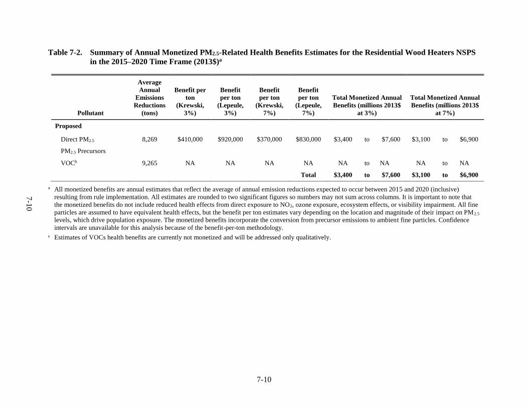
7-10
7-1
0
Table 7-2. Summary of Annual Monetized PM2.5-Related Health Benefits Estimates for the Residential Wood Heaters NSPS
in the 2015–2020 Time Frame (2013$)a
Pollutant
Average
Annual
Emissions
Reductions
(tons)
Benefit per
ton
(Krewski,
3%)
Benefit
per ton
(Lepeule,
3%)
Benefit
per ton
(Krewski,
7%)
Benefit
per ton
(Lepeule,
7%)
Total Monetized Annual
Benefits (millions 2013$
at 3%)
Total Monetized Annual
Benefits (millions 2013$
at 7%)
Proposed
Direct PM2.5 8,269 $410,000 $920,000 $370,000 $830,000 $3,400 to $7,600 $3,100 to $6,900
PM2.5 Precursors
VOCb 9,265 NA NA NA NA NA to NA NA to NA
Total $3,400 to $7,600 $3,100 to $6,900
a All monetized benefits are annual estimates that reflect the average of annual emission reductions expected to occur between 2015 and 2020 (inclusive)
resulting from rule implementation. All estimates are rounded to two significant figures so numbers may not sum across columns. It is important to note that
the monetized benefits do not include reduced health effects from direct exposure to NO2, ozone exposure, ecosystem effects, or visibility impairment. All fine
particles are assumed to have equivalent health effects, but the benefit per ton estimates vary depending on the location and magnitude of their impact on PM2.5
levels, which drive population exposure. The monetized benefits incorporate the conversion from precursor emissions to ambient fine particles. Confidence
intervals are unavailable for this analysis because of the benefit-per-ton methodology.
b Estimates of VOCs health benefits are currently not monetized and will be addressed only qualitatively.

7-11
Table 7-3. Summary of Reductions in Health Incidences from PM2.5-Related Benefits for
the Residential Wood Heaters NSPS in the 2015-2020 Time Framea
Health Incidences RWH NSPS
Avoided Premature Mortality
Krewski et al. (2009) (adult) 360
Lepeule et al. (2012) (adult) 810
Avoided Morbidity
Emergency department visits for asthma (all ages) 180
Acute bronchitis (age 8–12) 550
Lower respiratory symptoms (age 7–14) 7,000
Upper respiratory symptoms (asthmatics age 9–11) 10,000
Minor restricted-activity days (age 18–65) 280,000
Lost work days (age 18–65) 48,000
Asthma exacerbation (age 6–18) 25,000
Hospital admissions—respiratory (all ages) 92
Hospital admissions—cardiovascular (age > 18) 110
Non-Fatal Heart Attacks (age >18)
Peters et al. (2001) 390
Pooled estimate of 4 studies 42
a All estimates are rounded to whole numbers with two significant figures. Confidence intervals are unavailable for
this analysis because of the benefit-per-ton methodology.
the 12 functions supplied by experts. Figure 7-2 provides a breakdown of monetized benefits by
pollutant. In Table 7-4, we provide the benefits using our anchor points of Krewski et al., and
Lepeule et al., as well as the results from the 12 experts’ elicitation on PM mortality.
7.2.5 Characterization of Uncertainty in the Monetized PM2.5 Benefits
In any complex analysis using estimated parameters and inputs from numerous models,
there are likely to be many sources of uncertainty. This analysis is no exception. This analysis
includes many data sources as inputs, including emission inventories, air quality data from
models (with their associated parameters and inputs), population data, population estimates,
health effect estimates from epidemiology studies, economic data for monetizing benefits, and
assumptions regarding the future state of the world (i.e., regulations, technology, and human
behavior). Each of these inputs may be uncertain and would affect the benefits estimate. When
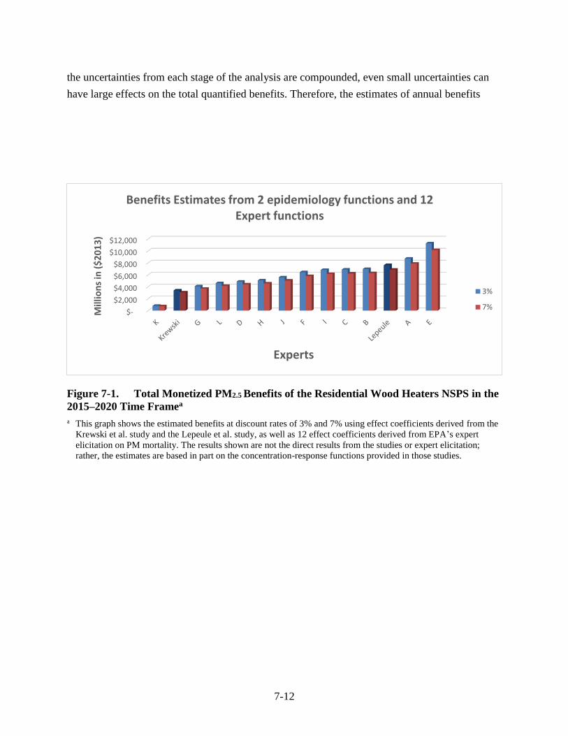
7-12
the uncertainties from each stage of the analysis are compounded, even small uncertainties can
have large effects on the total quantified benefits. Therefore, the estimates of annual benefits
Figure 7-1. Total Monetized PM2.5 Benefits of the Residential Wood Heaters NSPS in the
2015–2020 Time Framea
a This graph shows the estimated benefits at discount rates of 3% and 7% using effect coefficients derived from the
Krewski et al. study and the Lepeule et al. study, as well as 12 effect coefficients derived from EPA’s expert
elicitation on PM mortality. The results shown are not the direct results from the studies or expert elicitation;
rather, the estimates are based in part on the concentration-response functions provided in those studies.
$-
$2,000
$4,000
$6,000
$8,000
$10,000
$12,000
Mill
ion
s in
($
20
13
)
Experts
Benefits Estimates from 2 epidemiology functions and 12 Expert functions
3%
7%

7-13
Figure 7-2. Breakdown of Total Monetized PM2.5 Benefits of the Residential Wood
Heaters NSPS by Category
$14 , 1%
$280 , 8%
$2 , 0%$1,653 , 49%
$1,435 , 42%
$296 , 9%
Monetized Benefits Breakdown by Category for Residential Wood Heaters NSPS in Millions of $2013 (Krewski, 3%)
Wood Stoves
Single Burn Rate Stoves
Pellet Stoves
Furnace: indoor,cordwood
Hydronic HeatingSystems

7-14
Table 7-4. All PM2.5 Annual Benefits Estimates for the Residential Wood Heaters NSPS at
Discount Rates of 3% and 7% for the 2015 to 2020 Time Frame ($2013
millions)a
RWH NSPS
3% 7%
Benefit-per-ton Coefficients Derived from Epidemiology Literature
Krewski et al. $3,400 $3,100
Lepeule et al. $7,600 $6,900
Benefit-per-ton Coefficients Derived from Expert Elicitation
Expert A $8,700 $7,900
Expert B $7,000 $6,300
Expert C $6,900 $6,200
Expert D $4,900 $4,400
Expert E $11,000 $10,000
Expert F $6,400 $5,800
Expert G $4,100 $3,700
Expert H $5,000 $4,600
Expert I $7,200 $6,200
Expert J $5,600 $5,000
Expert K $810 $740
Expert L $4,600 $4,200
a All estimates are rounded to two significant figures. All estimates are annual estimates that reflect the average
annual estimates of PM2.5 emission reductions over the 2015 to 2020 timeframe. Estimates do not include
confidence intervals because they were derived through the benefit-per-ton technique described above. The
benefits estimates from the expert elicitation are provided as a reasonable characterization of the uncertainty in the
mortality estimates associated with the concentration-response function. Confidence intervals are unavailable for
this analysis because of the benefit-per-ton methodology.
should be viewed as representative of the magnitude of annual benefits expected, rather than the
actual benefits that would occur every year.
This RIA does not include the type of detailed uncertainty assessment found in the PM
NAAQS RIA (U.S. EPA, 2012a) because we lack the necessary air quality input and monitoring
data to run the benefits model. However, the results of the uncertainty analyses presented in the
PM NAAQS RIA can provide some information regarding the uncertainty inherent in the
benefits results presented in this analysis. Sensitivity analyses conducted for the PM NAAQS
RIA indicate that alternate cessation lag assumptions could change the PM2.5-related mortality

7-15
benefits discounted at 3% by between 10% and –27% and that alternate income growth
adjustments could change the PM2.5-related mortality benefits by between 33% and −14%.96
Unlike the PM NAAQS RIA, we do not have data on the specific location of the air
quality changes associated with this rulemaking. As such, it is not feasible to estimate the
proportion of benefits occurring in different locations, such as designated nonattainment areas.
Instead, we applied benefit-per-ton estimates, which reflect specific geographic patterns of
emissions reductions and specific air quality and benefits modeling assumptions for each sector
(US EPA, 2013). For example, these estimates do not reflect local variability in population
density, meteorology, exposure, baseline health incidence rates, or other local factors that might
lead to an over-estimate or under-estimate of the actual benefits of controlling PM precursors.
Use of these $/ton values to estimate benefits may lead to higher or lower benefit estimates than
if benefits were calculated based on direct air quality modeling. Great care should be taken in
applying these estimates to emission reductions occurring in any specific location, as these
reflect national or regional emission changes and therefore represent average benefits-per-ton
over the entire United States (EPA, 2013). The benefits-per-ton for emission reductions in
specific locations may be very different from the estimates presented here, and the approach
above did not yield benefit per-ton estimates at a sub-national level. To the extent that the
geographic distributions of the emissions reductions for this rule are different from the modeled
emissions, the benefits may be underestimated or overestimated. In general, there is inherently
more uncertainty for new sources, which may not be included in the emissions inventory, than
existing sources. For more information, see the TSD describing the calculation of these benefit-
per-ton estimates (U.S. EPA, 2013).
Our estimate of the total benefits is based on EPA’s interpretation of the best available
scientific literature and methods and supported by the SAB-HES and the NAS (NRC, 2002).
Below are key assumptions underlying the estimates for premature mortality, which accounts for
98% of the total monetized PM2.5 benefits:
1. We assume that all fine particles, regardless of their chemical composition, are
equally potent in causing premature mortality. This is an important assumption,
because PM2.5 varies considerably in composition across sources, but the scientific
evidence is not yet sufficient to allow differentiation of effect estimates by particle
type. The PM ISA concluded that “many constituents of PM2.5 can be linked with
multiple health effects, and the evidence is not yet sufficient to allow differentiation
96 http://www.epa.gov/ttn/ecas/regdata/RIAs/finalria.pdf (pp 6-16).
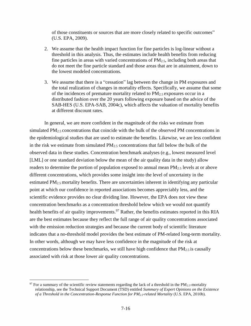
7-16
of those constituents or sources that are more closely related to specific outcomes”
(U.S. EPA, 2009).
2. We assume that the health impact function for fine particles is log-linear without a
threshold in this analysis. Thus, the estimates include health benefits from reducing
fine particles in areas with varied concentrations of PM2.5, including both areas that
do not meet the fine particle standard and those areas that are in attainment, down to
the lowest modeled concentrations.
3. We assume that there is a “cessation” lag between the change in PM exposures and
the total realization of changes in mortality effects. Specifically, we assume that some
of the incidences of premature mortality related to PM2.5 exposures occur in a
distributed fashion over the 20 years following exposure based on the advice of the
SAB-HES (U.S. EPA-SAB, 2004c), which affects the valuation of mortality benefits
at different discount rates.
In general, we are more confident in the magnitude of the risks we estimate from
simulated PM2.5 concentrations that coincide with the bulk of the observed PM concentrations in
the epidemiological studies that are used to estimate the benefits. Likewise, we are less confident
in the risk we estimate from simulated PM2.5 concentrations that fall below the bulk of the
observed data in these studies. Concentration benchmark analyses (e.g., lowest measured level
[LML] or one standard deviation below the mean of the air quality data in the study) allow
readers to determine the portion of population exposed to annual mean PM2.5 levels at or above
different concentrations, which provides some insight into the level of uncertainty in the
estimated PM2.5 mortality benefits. There are uncertainties inherent in identifying any particular
point at which our confidence in reported associations becomes appreciably less, and the
scientific evidence provides no clear dividing line. However, the EPA does not view these
concentration benchmarks as a concentration threshold below which we would not quantify
health benefits of air quality improvements.97 Rather, the benefits estimates reported in this RIA
are the best estimates because they reflect the full range of air quality concentrations associated
with the emission reduction strategies and because the current body of scientific literature
indicates that a no-threshold model provides the best estimate of PM-related long-term mortality.
In other words, although we may have less confidence in the magnitude of the risk at
concentrations below these benchmarks, we still have high confidence that PM2.5 is causally
associated with risk at those lower air quality concentrations.
97 For a summary of the scientific review statements regarding the lack of a threshold in the PM2.5-mortality
relationship, see the Technical Support Document (TSD) entitled Summary of Expert Opinions on the Existence
of a Threshold in the Concentration-Response Function for PM2.5-related Mortality (U.S. EPA, 2010b).

7-17
For this analysis, policy-specific air quality data is not available due to time or resource
limitations. For this rule, we are unable to estimate the percentage of premature mortality
associated with this specific rule’s emission reductions at each PM2.5 level. However, we believe
that it is still important to characterize the distribution of exposure to baseline air quality levels.
As a surrogate measure of mortality impacts, we provide the percentage of the population
exposed at each PM2.5 level in the baseline of the source apportionment modeling used to
calculate the benefit-per-ton estimates for this sector. It is important to note that baseline
exposure is only one parameter in the health impact function, along with baseline incidence rates
population, and change in air quality. In other words, the percentage of the population exposed to
air pollution below the LML is not the same as the percentage of the population experiencing
health impacts as a result of a specific emission reduction policy. The most important aspect,
which we are unable to quantify for rules without rule-specific air quality modeling, is the shift
in exposure associated with this specific rule. Therefore, caution is warranted when interpreting
the LML assessment for this rule because these results are not consistent with results from rules
that had air quality modeling.
Table 7-5 provides the percentage of the population exposed above and below two
concentration benchmarks (i.e., LML and 1 standard deviation below the mean) in the modeled
baseline. Figure 7-3 shows a bar chart of the percentage of the population exposed to various air
quality levels in the baseline, and Figure 7-4 shows a cumulative distribution function of the
same data. Both figures identify the LML for each of the major cohort studies.
7.3 Unquantified Benefits
The monetized benefits estimated in this RIA only reflect a subset of benefits attributable
to the health effect reductions associated with ambient fine particles. Data, time, and resource
limitations prevented EPA from quantifying the impacts to, or monetizing the benefits from
several important benefit categories, including benefits associated with the potential exposure to
ozone formation due to VOC emissions as a precursor, VOC emissions as a PM2.5 precursor,
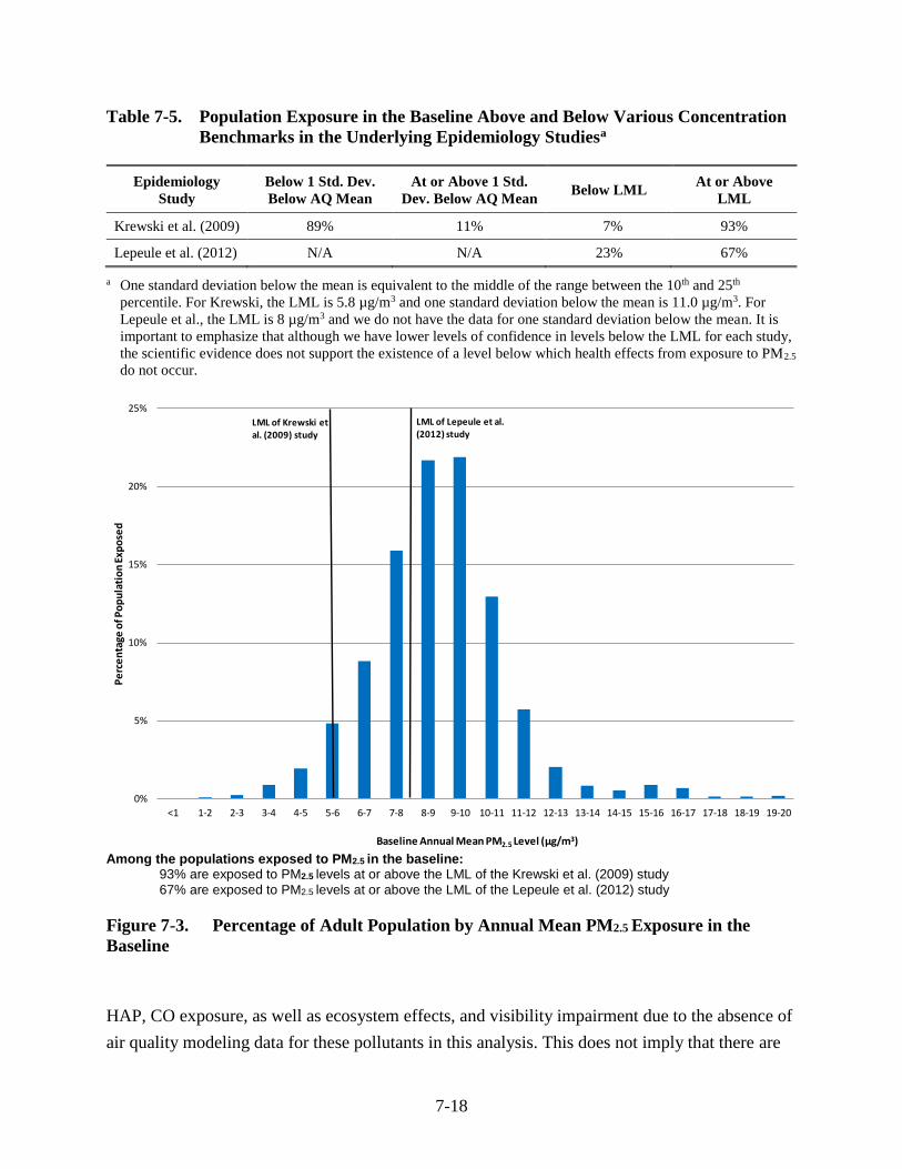
7-18
Table 7-5. Population Exposure in the Baseline Above and Below Various Concentration
Benchmarks in the Underlying Epidemiology Studiesa
Epidemiology
Study
Below 1 Std. Dev.
Below AQ Mean
At or Above 1 Std.
Dev. Below AQ Mean Below LML
At or Above
LML
Krewski et al. (2009) 89% 11% 7% 93%
Lepeule et al. (2012) N/A N/A 23% 67%
a One standard deviation below the mean is equivalent to the middle of the range between the 10th and 25th
percentile. For Krewski, the LML is 5.8 µg/m3 and one standard deviation below the mean is 11.0 µg/m3. For
Lepeule et al., the LML is 8 µg/m3 and we do not have the data for one standard deviation below the mean. It is
important to emphasize that although we have lower levels of confidence in levels below the LML for each study,
the scientific evidence does not support the existence of a level below which health effects from exposure to PM2.5
do not occur.
Among the populations exposed to PM2.5 in the baseline:
93% are exposed to PM2.5 levels at or above the LML of the Krewski et al. (2009) study
67% are exposed to PM2.5 levels at or above the LML of the Lepeule et al. (2012) study
Figure 7-3. Percentage of Adult Population by Annual Mean PM2.5 Exposure in the
Baseline
HAP, CO exposure, as well as ecosystem effects, and visibility impairment due to the absence of
air quality modeling data for these pollutants in this analysis. This does not imply that there are
0%
5%
10%
15%
20%
25%
<1 1-2 2-3 3-4 4-5 5-6 6-7 7-8 8-9 9-10 10-11 11-12 12-13 13-14 14-15 15-16 16-17 17-18 18-19 19-20
Pe
rce
nta
ge o
f Po
pu
lati
on
Exp
ose
d
Baseline Annual Mean PM2.5 Level (µg/m3)
Percentage of Population Exposed by Baseline Air Quality Level
LML of Lepeule et al. (2012) study
LML of Krewski et al. (2009) study

7-19
no benefits associated with these emission reductions. In this section, we provide a qualitative
description of these benefits.
7.3.1 HAP Benefits
When looking at exposures from all air toxic sources of outdoor origin across the U.S.,
we see that emissions have declined by approximately 42% since 1990. However, despite this
declines, the 2005 National-Scale Air Toxics Assessment (NATA), which includes emissions
from residential wood heater, predicts that many Americans are exposed to ambient
concentrations of air toxics at levels that may have the potential to cause adverse health effects
(U.S. EPA, 2011c).98 The levels of air toxics to which people are exposed vary depending on
where people live and work and the kinds of activities in which they engage. In order to identify
and prioritize air toxics, emission source types and locations that are of greatest potential
concern, U.S. EPA conducts the National Air Toxic Analysis (NATA).99 The most recent NATA
was conducted for calendar year 2005 and was released in March 2011. NATA includes four
steps:
98 The 2005 NATA is available on the Internet at http://www.epa.gov/ttn/atw/nata2005/. 99 The NATA modeling framework has a number of limitations that prevent its use as the sole basis for setting
regulatory standards. These limitations and uncertainties are discussed on the 2005 NATA website. Even so, this
modeling framework is very useful in identifying air toxic pollutants and sources of greatest concern, setting
regulatory priorities, and informing the decision making process. U.S. EPA.(2011). 2005 National-Scale Air
Toxics Assessment. http://www.epa.gov/ttn/atw/nata2005/

7-20
Among the populations exposed to PM2.5 in the baseline: 93% are exposed to PM2.5 levels at or above the LML of the Krewski et al. (2009) study
67% are exposed to PM2.5 levels at or above the LML of the Lepeule et al. (2012) study
Figure 7-4. Cumulative Distribution of Adult Population by Annual Mean PM2.5
Exposure in the Baseline
1. Compiling a national emissions inventory of air toxics emissions from outdoor
sources
2. Estimating ambient concentrations of air toxics across the United States
3. Estimating population exposures across the United States utilizing exposure models
4. Characterizing potential public health risk due to inhalation of air toxics including
both cancer and noncancer effects
Based on the 2005 NATA, EPA estimates that about 5% of census tracts nationwide have
increased cancer risks greater than 100 in a million. The average national cancer risk is about 50
in a million. Nationwide, the key pollutants that contribute most to the overall cancer risks are
0%
10%
20%
30%
40%
50%
60%
70%
80%
90%
100%
1 2 3 4 5 6 7 8 9 10 11 12 13 14 15 16 17 18 19 20
Cu
mu
lati
ve p
erc
en
tage
of p
op
ula
tio
n e
xpo
sed
Baseline Annual Mean PM2.5 Level (µg/m3)
Cumulative Percentage of Population Exposed by Baseline Air Quality Level
LML of Krewski et al. (2009) study
LML of Lepeule et al. (2012) study
7-21
formaldehyde and benzene.100 Secondary formation (e.g., formaldehyde forming from other
emitted pollutants) was the largest contributor to cancer risks, while stationary, mobile and
background sources contribute almost equal portions of the remaining cancer risk.
Noncancer health effects can result from chronic,101 subchronic,102 or acute103 inhalation
exposures to air toxics, and include neurological, cardiovascular, liver, kidney, and respiratory
effects as well as effects on the immune and reproductive systems. According to the 2005
NATA, about three-fourths of the U.S. population was exposed to an average chronic
concentration of air toxics that has the potential for adverse noncancer respiratory health effects.
Results from the 2005 NATA indicate that acrolein is the primary driver for noncancer
respiratory risk.
Figures 7-5 and 7-6 depict the 2005 NATA estimated census tract-level carcinogenic risk
and noncancer respiratory hazard from the assessment. It is important to note that large
reductions in HAP emissions may not necessarily translate into significant reductions in health
risk because toxicity varies by pollutant, and exposures may or may not exceed levels of
concern. For example, acetaldehyde mass emissions are more than double acrolein emissions on
a national basis, according to EPA’s 2005 National Emissions Inventory (NEI). However, the
Integrated Risk Information System (IRIS) reference concentration (RfC) for acrolein is
considerably lower
100 Details about the overall confidence of certainty ranking of the individual pieces of NATA assessments including
both quantitative (e.g., model-to-monitor ratios) and qualitative (e.g., quality of data, review of emission
inventories) judgments can be found at http://www.epa.gov/ttn/atw/nata/roy/page16.html. 101 Chronic exposure is defined in the glossary of the Integrated Risk Information (IRIS) database
(http://www.epa.gov/iris ) as repeated exposure by the oral, dermal, or inhalation route for more than
approximately 10% of the life span in humans (more than approximately 90 days to 2 years in typically used
laboratory animal species). 102 Defined in the IRIS database as repeated exposure by the oral, dermal, or inhalation route for more than 30 days,
up to approximately 10% of the life span in humans (more than 30 days up to approximately 90 days in typically
used laboratory animal species). 103 Defined in the IRIS database as exposure by the oral, dermal, or inhalation route for 24 hours or less.

7-22
Figure 7-5. 2005 NATA Model Estimated Census Tract Carcinogenic Risk from HAP
Exposure from Emissions of All Outdoor Sources (inclusive of Residental Wood Heaters)
based on the 2005 National Toxic Inventory
than that for acetaldehyde, suggesting that acrolein could be potentially more toxic than
acetaldehyde. Thus, it is important to account for the toxicity and exposure, as well as the mass
of the targeted emissions.
Due to methodology limitations, we were unable to estimate the benefits associated with
the hazardous air pollutants that would be reduced as a result of this rule. In a few previous
analyses of the benefits of reductions in HAP, EPA has quantified the benefits of potential
reductions in the incidences of cancer and non-cancer risk (e.g., U.S. EPA, 1995). In those
analyses, EPA relied on unit risk factors (URF) and reference concentrations (RfC) developed
through risk assessment procedures. The URF is a quantitative estimate of the carcinogenic
potency of a pollutant, often expressed as the probability of contracting cancer from a 70-year

7-23
lifetime continuous exposure to a concentration of one µg/m3 of a pollutant .104These URFs are
designed to be conservative, and as such, are more likely to
104 The unit risk factor is a quantitative estimate of the carcinogenic potency of a pollutant, often expressed as the
probability of contracting cancer from a 70-year lifetime continuous exposure to a concentration of one µg/m3 of
a pollutant.

7-24
Figure 7-6. 2005 NATA Model Estimated Census Tract Noncancer Risk from HAP
Exposure from Emissions of All Outdoor Sources (inclusive of Residental Wood Heaters)
based on the 2005 National Toxic Inventory
represent the high end of the distribution of risk rather than a best or most likely estimate of risk.
An RfC is an estimate (with uncertainty spanning perhaps an order of magnitude) of a
continuous inhalation exposure to the human population (including sensitive subgroups) that is
likely to be without an appreciable risk of deleterious noncancer health effects during a lifetime.
As the purpose of a benefit analysis is to describe the benefits most likely to occur from a
reduction in pollution, use of high-end, conservative risk estimates would overestimate the
benefits of the regulation. While we used high-end risk estimates in past analyses, advice from
the EPA’s Science Advisory Board (SAB) recommended that we avoid using high-end estimates
in benefit analyses (U.S. EPA-SAB, 2002). Since this time, EPA has continued to develop better
methods for analyzing the benefits of reductions in HAP.
As part of the second prospective analysis of the benefits and costs of the Clean Air Act
(U.S. EPA, 2011a), EPA conducted a case study analysis of the health effects associated with
7-25
reducing exposure to benzene in Houston from implementation of the Clean Air Act (IEc, 2009).
While reviewing the draft report, EPA’s Advisory Council on Clean Air Compliance Analysis
concluded that “the challenges for assessing progress in health improvement as a result of
reductions in emissions of hazardous air pollutants (HAPs) are daunting…due to a lack of
exposure-response functions, uncertainties in emissions inventories and background levels, the
difficulty of extrapolating risk estimates to low doses and the challenges of tracking health
progress for diseases, such as cancer, that have long latency periods” (U.S. EPA-SAB, 2008).
In 2009, EPA convened a workshop to address the inherent complexities, limitations, and
uncertainties in current methods to quantify the benefits of reducing HAP. Recommendations
from this workshop included identifying research priorities, focusing on susceptible and
vulnerable populations, and improving dose-response relationships (Gwinn et al., 2011).
In summary, monetization of the benefits of reductions in cancer incidences requires
several important inputs, including central estimates of cancer risks, estimates of exposure to
carcinogenic HAP, and estimates of the value of an avoided case of cancer (fatal and non-fatal).
Due to methodology limitations, we did not attempt to monetize the health benefits of reductions
in HAP in this analysis. Instead, we provide a qualitative analysis of the health effects associated
with the HAP anticipated to be reduced by these rules. EPA remains committed to improving
methods for estimating HAP benefits by continuing to explore additional concepts of benefits,
including changes in the distribution of risk.
Below we describe the health effects associated with the HAPs that would be reduced by
this rulemaking.
7.3.1.1 Benzene
The EPA’s IRIS database lists benzene as a known human carcinogen (causing leukemia)
by all routes of exposure, and concludes that exposure is associated with additional health effects,
including genetic changes in both humans and animals and increased proliferation of bone marrow

7-26
cells in mice.105,106,107 EPA states in its IRIS database that data indicate a causal relationship
between benzene exposure and acute lymphocytic leukemia and suggest a relationship between
benzene exposure and chronic non-lymphocytic leukemia and chronic lymphocytic leukemia. The
IARC has determined that benzene is a human carcinogen and the U.S. Department of Health and
Human Services has characterized benzene as a known human carcinogen.108,109
A number of adverse noncancer health effects including blood disorders, such as
preleukemia and aplastic anemia, have also been associated with long-term exposure to
benzene.110,111
7.3.1.2 Dioxins (Chlorinated dibenzodioxins (CDDs)112
Exposure to 2,3,7,8- tetrachlorodibenzo-p-dioxin (2,3,7,8-TCDD) at high enough levels
may cause a number of adverse health effects. The most obvious noncancer health effect in
people exposed to relatively large amounts of 2,3,7,8-TCDD is Chloracne. Chloracne is a severe
skin disease with acne-like lesions that occur mainly on the face and upper body. Other skin
effects noted in people exposed to high doses of 2,3,7,8-TCDD include skin rashes,
discoloration, and excessive body hair. Exposure to large amounts of dioxin may also induce
other noncancer effects including developmental and reproductive effects, damage to the
immune system, interference with hormones and possibly mild liver damage.
105 U.S. Environmental Protection Agency (U.S. EPA). 2000. Integrated Risk Information System File for Benzene.
Research and Development, National Center for Environmental Assessment, Washington, DC. This material is
available electronically at: http://www.epa.gov/iris/subst/0276.htm. 106 International Agency for Research on Cancer, IARC monographs on the evaluation of carcinogenic risk of
chemicals to humans, Volume 29, Some industrial chemicals and dyestuffs, International Agency for Research
on Cancer, World Health Organization, Lyon, France, p. 345-389, 1982. 107 Irons, R.D.; Stillman, W.S.; Colagiovanni, D.B.; Henry, V.A. (1992) Synergistic action of the benzene metabolite
hydroquinone on myelopoietic stimulating activity of granulocyte/macrophage colony-stimulating factor in vitro,
Proc. Natl. Acad. Sci. 89:3691-3695. 108 International Agency for Research on Cancer (IARC). 1987. Monographs on the evaluation of carcinogenic risk
of chemicals to humans, Volume 29, Supplement 7, Some industrial chemicals and dyestuffs, World Health
Organization, Lyon, France. 109 U.S. Department of Health and Human Services National Toxicology Program 11th Report on Carcinogens
available at: http://ntp.niehs.nih.gov/go/16183 . 110 Aksoy, M. (1989). Hematotoxicity and carcinogenicity of benzene. Environ. Health Perspect. 82: 193-197. 111 Goldstein, B.D. (1988). Benzene toxicity. Occupational medicine. State of the Art Reviews. 3: 541-554. 112 The health effects language for this section came from: EPA’s Dioxin Assessment Consumer Fact Sheet,
available at http://www.epa.gov/dioxin/pdfs/EPA-Dioxin-Factsheet-2012.pdf, and Agency for Toxic Substances
and Disease Registry (ATSDR). 1999. ToxFAQs for Chlorinated Dibenzo-p-dioxins (CDDs) (CAS#: 2,3,7,8-
TCDD 1746-01-6). Atlanta, GA: U.S. Department of Health and Human Services, Public Health Service.
Available at http://www.atsdr.cdc.gov/tfacts104.html.
7-27
The EPA has classified 2,3,7,8 TCDD as carcinogenic to humans in accordance with
EPA’s 2005 Guidelines for Carcinogenic Risk Assessment.113 IARC and NTP have classified
2,3,7,8 TCDD as Group 1 (carcinogenic to humans)114 and known human carcinogen115,
respectively.
7.3.1.3 Formaldehyde
Since 1987, EPA has classified formaldehyde as a probable human carcinogen based on
evidence in humans and in rats, mice, hamsters, and monkeys.116 Substantial additional research
since that time informs current scientific understanding of the health effects associated with
exposure to formaldehyde. These include recently published research conducted by the National
Cancer Institute (NCI) which found an increased risk of nasopharyngeal cancer and
lymphohematopoietic malignancies such as leukemia among workers exposed to
formaldehyde.117,118 In an analysis of the lymphohematopoietic cancer mortality from an
extended follow-up of these workers, NCI confirmed an association between
lymphohematopoietic cancer risk and peak formaldehyde exposures.119 A recent NIOSH study of
garment workers also found increased risk of death due to leukemia among workers exposed to
formaldehyde.120 Extended follow-up of a cohort of British chemical workers did not find
evidence of an increase in nasopharyngeal or lymphohematopoietic cancers, but a continuing
statistically significant excess in lung cancers was reported.121
113 U.S. EPA. 2012. EPA’s Reanalysis of Key Issues Related to Dioxin Toxicity and Response to NAS Comments
Volume 1. EPA/600/R-10?038F. Available at: http://www.epa.gov/iris/supdocs/dioxinv1sup.pdf. 114 International Agency for Research on Cancer (IARC). IARC Monographs on the Evaluation of Carcinogenic
Risks to Humans, 2012. Available at: http://monographs.iarc.fr/ENG/Classification/index.php. 115 U.S. Department of Health and Human Services. National Toxicology Program.13th Report on the Carcinogens
(RoC). Available at: http://ntp.niehs.nih.gov/ntp/roc/content/listed_substances_508.pdf. 116 U.S. EPA. 1987. Assessment of Health Risks to Garment Workers and Certain Home Residents from Exposure to
Formaldehyde, Office of Pesticides and Toxic Substances, April 1987. Docket EPA-HQ-OAR-2010-0162. 117 Hauptmann, M.; Lubin, J. H.; Stewart, P. A.; Hayes, R. B.; Blair, A. 2003. Mortality from lymphohematopoetic
malignancies among workers in formaldehyde industries. Journal of the National Cancer Institute 95: 1615-1623.
Docket EPA-HQ-OAR-2010-0162. 118 Hauptmann, M.; Lubin, J. H.; Stewart, P. A.; Hayes, R. B.; Blair, A. 2004. Mortality from solid cancers among
workers in formaldehyde industries. American Journal of Epidemiology 159: 1117-1130. Docket EPA-HQ-
OAR-2010-0162. 119 Beane Freeman, L. E.; Blair, A.; Lubin, J. H.; Stewart, P. A.; Hayes, R. B.; Hoover, R. N.; Hauptmann, M. 2009.
Mortality from lymphohematopoietic malignancies among workers in formaldehyde industries: The National
Cancer Institute cohort. J. National Cancer Inst. 101: 751-761. Docket EPA-HQ-OAR-2010-0162. 120 Pinkerton, L. E. 2004. Mortality among a cohort of garment workers exposed to formaldehyde: an update. Occup.
Environ. Med. 61: 193-200. Docket EPA-HQ-OAR-2010-0162. 121 Coggon, D, EC Harris, J Poole, KT Palmer. 2003. Extended follow-up of a cohort of British chemical workers
exposed to formaldehyde. J National Cancer Inst. 95:1608-1615. Docket EPA-HQ-OAR-2010-0162.
7-28
In the past 15 years there has been substantial research on the inhalation dosimetry for
formaldehyde in rodents and primates by the Chemical Industry Institute of Toxicology (CIIT,
now renamed the Hamner Institutes for Health Sciences), with a focus on use of rodent data for
refinement of the quantitative cancer dose-response assessment.122,123,124 CIIT’s risk assessment
of formaldehyde incorporated mechanistic and dosimetric information on formaldehyde. These
data were modeled using a biologically-motivated two-stage clonal growth model for cancer and
also a point of departure based on a Benchmark Dose approach. However, it should be noted that
recent research published by EPA indicates that when two-stage modeling assumptions are
varied, resulting dose-response estimates can vary by several orders of magnitude.125,126,127,128
These findings are not supportive of interpreting the CIIT model results as providing a
conservative (health protective) estimate of human risk.129 EPA research also examined the
contribution of the two-stage modeling for formaldehyde towards characterizing the relative
weights of key events in the mode-of-action of a carcinogen. For example, the model-based
inference in the published CIIT study that formaldehyde’s direct mutagenic action is not relevant
to the compound’s tumorigenicity was found not to hold under variations of modeling
assumptions.130
122 Conolly, RB, JS Kimbell, D Janszen, PM Schlosser, D Kalisak, J Preston, and FJ Miller. 2003. Biologically
motivated computational modeling of formaldehyde carcinogenicity in the F344 rat. Tox Sci 75: 432-447.
Docket EPA-HQ-OAR-2010-0162. 123 Conolly, RB, JS Kimbell, D Janszen, PM Schlosser, D Kalisak, J Preston, and FJ Miller. 2004. Human
respiratory tract cancer risks of inhaled formaldehyde: Dose-response predictions derived from biologically-
motivated computational modeling of a combined rodent and human dataset. Tox Sci 82: 279-296. Docket EPA-
HQ-OAR-2010-0162. 124 Chemical Industry Institute of Toxicology (CIIT).1999. Formaldehyde: Hazard characterization and dose-
response assessment for carcinogenicity by the route of inhalation. CIIT, September 28, 1999. Research Triangle
Park, NC. Docket EPA-HQ-OAR-2010-0162. 125 U.S. EPA. Analysis of the Sensitivity and Uncertainty in 2-Stage Clonal Growth Models for Formaldehyde with
Relevance to Other Biologically-Based Dose Response (BBDR) Models. U.S. Environmental Protection Agency,
Washington, D.C., EPA/600/R-08/103, 2008. Docket EPA-HQ-OAR-2010-0162. 126 Subramaniam, R; Chen, C; Crump, K; et al. (2008) Uncertainties in biologically-based modeling of
formaldehyde-induced cancer risk: identification of key issues. Risk Anal 28(4):907-923. Docket EPA-HQ-
OAR-2010-0162. 127 Subramaniam RP; Crump KS; Van Landingham C; et al. (2007) Uncertainties in the CIIT model for
formaldehyde-induced carcinogenicity in the rat: A limited sensitivity analysis–I. Risk Anal, 27: 1237–1254.
Docket EPA-HQ-OAR-2010-0162. 128 Crump, K; Chen, C; Fox, J; et al. (2008) Sensitivity analysis of biologically motivated model for formaldehyde-
induced respiratory cancer in humans. Ann Occup Hyg 52:481-495. Docket EPA-HQ-OAR-2010-0162. 129 Crump, K; Chen, C; Fox, J; et al. (2008) Sensitivity analysis of biologically motivated model for formaldehyde-
induced respiratory cancer in humans. Ann Occup Hyg 52:481-495. Docket EPA-HQ-OAR-2010-0162. 130 Subramaniam RP; Crump KS; Van Landingham C; et al. (2007) Uncertainties in the CIIT model for
formaldehyde-induced carcinogenicity in the rat: A limited sensitivity analysis–I. Risk Anal, 27: 1237–1254.
Docket EPA-HQ-OAR-2010-0162.
7-29
Based on the developments of the last decade, in 2004, the working group of the IARC
concluded that formaldehyde is carcinogenic to humans (Group 1), on the basis of sufficient
evidence in humans and sufficient evidence in experimental animals—a higher classification
than previous IARC evaluations. After reviewing the currently available epidemiological
evidence, the IARC (2006) characterized the human evidence for formaldehyde carcinogenicity
as “sufficient,” based upon the data on nasopharyngeal cancers; the epidemiologic evidence on
leukemia was characterized as “strong.”131 The NTP has classified formaldehyde as “known to be
human carcinogen.” 132
Formaldehyde exposure also causes a range of noncancer health effects, including
irritation of the eyes (burning and watering of the eyes), nose and throat. Effects from repeated
exposure in humans include respiratory tract irritation, chronic bronchitis and nasal epithelial
lesions such as metaplasia and loss of cilia. Animal studies suggest that formaldehyde may also
cause airway inflammation—including eosinophils infiltration into the airways. There are several
studies that suggest that formaldehyde may increase the risk of asthma—particularly in the
young.133,134
The above-mentioned rodent and human studies, as well as mechanistic information and
their analyses, were evaluated in EPA’s recent Draft Toxicological Review of Formaldehyde—
Inhalation Assessment through the Integrated Risk Information System (IRIS) program. This
draft IRIS assessment was released in June 2010 for public review and comment and external
peer review by the National Research Council (NRC). The NRC released their review report in
April 2011 (http://www.nap.edu/catalog.php?record_id=13142). The EPA is currently revising
the draft assessment in response to this review.
131 International Agency for Research on Cancer (2006) Formaldehyde, 2-Butoxyethanol and 1-tert-Butoxypropan-2-
ol. Monographs Volume 88. World Health Organization, Lyon, France. Docket EPA-HQ-OAR-2010-0162. 132 U.S. Department of Health and Human Services. National Toxicology Program.13th Report on the Carcinogens
(RoC). Available at: http://ntp.niehs.nih.gov/pubhealth/roc/roc13/index.html#F
133 Agency for Toxic Substances and Disease Registry (ATSDR). 1999. Toxicological profile for Formaldehyde.
Atlanta, GA: U.S. Department of Health and Human Services, Public Health Service.
http://www.atsdr.cdc.gov/toxprofiles/tp111.html. Docket EPA-HQ-OAR-2010-0162. 134 WHO (2002) Concise International Chemical Assessment Document 40: Formaldehyde. Published under the
joint sponsorship of the United Nations Environment Programme, the International Labour Organization, and the
World Health Organization, and produced within the framework of the Inter-Organization Programme for the
Sound Management of Chemicals. Geneva. Docket EPA-HQ-OAR-2010-0162.

7-30
7.3.1.4 Polycyclic Organic Matter (POM)
The term polycyclic organic matter (POM) defines a broad class of compounds that
includes the polycyclic aromatic hydrocarbon compounds (PAHs). One of these compounds,
naphthalene, is discussed separately below. POM compounds are formed primarily from
combustion and are present in the atmosphere in gas and particulate form. Cancer is the major
concern from exposure to POM. Epidemiologic studies have reported an increase in lung cancer
in humans exposed to diesel exhaust, coke oven emissions, roofing tar emissions, and cigarette
smoke; all of these mixtures contain POM compounds135,136. Animal studies have reported
respiratory tract tumors from inhalation exposure to benzo[a]pyrene and alimentary tract and
liver tumors from oral exposure to benzo[a]pyrene. EPA has classified seven PAHs
(benzo[a]pyrene, benz[a]anthracene, chrysene, benzo[b]fluoranthene, benzo[k]fluoranthene,
dibenz[a,h]anthracene, and indeno[1,2,3-cd]pyrene) as Group B2, probable human
carcinogens.137 Recent studies have found that maternal exposures to PAHs in a population of
pregnant women were associated with several adverse birth outcomes, including low birth
weight and reduced length at birth, as well as impaired cognitive development in preschool
children (3 years of age).138,139 EPA has not yet evaluated these recent studies.
7.3.1.5 Other Air Toxics
In addition to the compounds described above, other air toxic compounds would be
affected by this rule. Information regarding the health effects of these compounds can be found
in EPA’s IRIS database.140
7.3.2 Carbon Monoxide Co-Benefits
Carbon monoxide in ambient air is formed primarily by the incomplete combustion of
carbon-containing fuels and photochemical reactions in the atmosphere. The amount of CO
emitted from these reactions, relative to carbon dioxide (CO2), is sensitive to conditions in the
135 Agency for Toxic Substances and Disease Registry (ATSDR). 1995. Toxicological profile for Polycyclic
Aromatic Hydrocarbons (PAHs). Atlanta, GA: U.S. Department of Health and Human Services, Public Health
Service. Available electronically at http://www.atsdr.cdc.gov/ToxProfiles/TP.asp?id=122&tid=25. 136 U.S. EPA (2002). Health Assessment Document for Diesel Engine Exhaust. EPA/600/8-90/057F Office of
Research and Development, Washington DC. Retrieved on March 17, 2009 from
http://cfpub.epa.gov/ncea/cfm/recordisplay.cfm?deid=29060. Docket EPA-HQ-OAR-2010-0162. 137 U.S. EPA (1997). Integrated Risk Information System File of indeno(1,2,3-cd)pyrene. Research and
Development, National Center for Environmental Assessment, Washington, DC. This material is available
electronically at http://www.epa.gov/ncea/iris/subst/0457.htm. 138 Perera, F.P.; Rauh, V.; Tsai, W-Y.; et al. (2002) Effect of transplacental exposure to environmental pollutants on
birth outcomes in a multiethnic population. Environ Health Perspect. 111: 201-205. 139 Perera, F.P.; Rauh, V.; Whyatt, R.M.; Tsai, W.Y.; Tang, D.; Diaz, D.; Hoepner, L.; Barr, D.; Tu, Y.H.; Camann,
D.; Kinney, P. (2006) Effect of prenatal exposure to airborne polycyclic aromatic hydrocarbons on
neurodevelopment in the first 3 years of life among inner-city children. Environ Health Perspect 114: 1287-1292. 140 U.S. EPA Integrated Risk Information System (IRIS) database is available at: www.epa.gov/iris.

7-31
combustion zone, such as fuel oxygen content, burn temperature, or mixing time. Upon
inhalation, CO diffuses through the respiratory system to the blood, which can cause hypoxia
(reduced oxygen availability). Carbon monoxide can elicit a broad range of effects in multiple
tissues and organ systems that are dependent upon concentration and duration of exposure. The
Integrated Science Assessment for Carbon Monoxide (U.S. EPA, 2010a) concluded that short-
term exposure to CO is “likely to have a causal relationship” with cardiovascular morbidity,
particularly in individuals with coronary heart disease. Epidemiologic studies associate short-
term CO exposure with increased risk of emergency department visits and hospital admissions.
Coronary heart disease includes those who have angina pectoris (cardiac chest pain), as well as
those who have experienced a heart attack. Other subpopulations potentially at risk include
individuals with diseases such as chronic obstructive pulmonary disease (COPD), anemia, or
diabetes, and individuals in very early or late life stages, such as older adults or the developing
young. The evidence is suggestive of a causal relationship between short-term exposure to CO
and respiratory morbidity and mortality. The evidence is also suggestive of a causal relationship
for birth outcomes and developmental effects following long-term exposure to CO, and for
central nervous system effects linked to short- and long-term exposure to CO.
7.3.3 Black Carbon (BC) Benefits
Incomplete combustion of wood results in emissions of fine and ultrafine particles,
including black carbon (BC), brown carbon (BrC), and other non-light-absorbing organic carbon
(OC) particles. BC and BrC are collectively considered light-absorbing carbon (LAC) with BC
referring to the most strongly light‐absorbing form of carbon per unit mass. BC impacts the
earth’s climate because of its high capacity for light absorption. The role of BC in key
atmospheric processes links it to a range of climate impacts, including increased temperatures,
accelerated ice and snow melt, and disruptions in precipitation patterns. A recent study by the
UN Environment Programme (UNEP) concluded that reductions in BC and ozone will slow the
rate of climate change within the first half of this century with a small number of targeted BC
and ozone precursor emissions mitigation measures providing immediate protection for climate,
public health, water and food security, and ecosystems (UNEP, 2011).141
While less effective in absorbing solar radiation than BC, BrC may contribute
significantly to positive radiative forcing. At present the ability to quantify the climate impacts of
BrC is limited. OC from incomplete combustion of wood (exclusive of BrC) is generally
141 UN Environment Programme, World Meteorological Organization. 2011, February. Integrated Assessment of
Black Carbon and Tropospheric Ozone: Summary for Decision Makers. Available at
http://www.unep.org/gc/gc26/download.asp?ID=2197.

7-32
considered non-light‐absorbing carbon. Non-light-absorbing compounds scatter rather than
absorb solar radiation and, therefore, provide a net direct cooling effect on climate. Thus,
particles generated by residential wood combustion consist of components that are warming to
the atmosphere (BC and BrC) and particles that are cooling (OC exclusive of BrC).
Residential wood combustion contributed about 380,000 tons of PM2.5 emissions across
the United States in 2005. Of these PM2.5 emissions, approximately 21,000 tons are estimated to
7-33
be elemental carbon (EC)142 (EPA NEI, 2005).143
The EC/OC ratio is a metric sometimes used to crudely compare the warming potential of
emissions from various BC sources with a ratio of less than 1 indicating that cooling potential
exceeds warming. Based on the speciated 2005 NEI, the EC/OC for residential wood combustion
is estimated to be less than one (~ 0.11), indicating a predominance of OC or light-scattering
particles relative to light absorbing ones. Exactly how much of the OC from RWC sources is
light absorbing (BrC) is not known currently, and the LAC may vary by fuel type, combustion
conditions, and operating environment.
While OC emissions are generally considered to have a cooling effect, OC emissions
over areas with snow and ice may be less reflective than OC over dark surfaces and may even
have a slight warming effect (Flanner et al., 2007).144 Significantly, the vast majority of
residential wood smoke emissions occur during the winter months; the highest percentage of
wood stove use is in the upper Midwest (e.g., Michigan), the Northeast (e.g., Maine), and the
mountainous areas of the Pacific Northwest (e.g., Washington), where snow is present a good
portion of the winter months. A recent study of the effect of soot-induced snow albedo on
snowpack and hydrological cycles in the western United States concludes that radiative forcing
induced by soot deposition on snow is an important anthropogenic source affecting the global
climate. The study concludes that soot-induced snow albedo perturbations increase the surface
net solar radiation flux during late winter to early spring, increase the surface air temperature,
reduce the snow accumulation and spring snowmelt, and may alter stream flows with
implications for water resources in the western United States (Qian, et al., 2009).145 Further study
is needed to better understand and quantify the impact of PM2.5 emissions and deposition from
the RWC sector on climate.
7.3.4 VOCs as a PM2.5 Precursor
This rulemaking is expected to reduce emissions of VOCs, which are a precursor to
PM2.5. Most VOCs emitted are oxidized to carbon dioxide (CO2) rather than to PM, but a portion
142 BC is roughly equivalent to ‘soot carbon’ or the portion of soot that is closest to elemental carbon. The most
commonly used measurement technique, the ‘thermal optical method’ quantifies the portion of PM that is EC.
EC is frequently used for emissions characterization and ambient measurements. The terms EC and BC are used
interchangeably in this discussion. 143 U.S. EPA. 2005. National Emissions Inventory. 2005 Modeling Inventory. Available at.
http://www.epa.gov/ttn/chief/emch/index.html. 144 Flanner, M. G., Zender, C. S., Randerson, J. T., and Rasch, P. J. 2007. Present‐day climate forcing and response
from BC in snow. Journal of Geophysical Research-Atmospheres, 12(D11). doi:10.1029/2006JD008003 145 Qian, Y., W. I. Gustafson, L. R. Leung, and S. J. Ghan. 2009. Effects of soot‐induced snow albedo change on
snowpack and hydrological cycle in western United States based on Weather Research and Forecasting
chemistry and regional climate simulations, J. Geophys. Res. 114, D03108. doi:10.1029/2008JD011039

7-34
of VOC emission contributes to ambient PM2.5 levels as organic carbon aerosols (U.S. EPA,
2009c). Therefore, reducing these emissions would reduce PM2.5 formation, human exposure to
PM2.5, and the incidence of PM2.5-related health effects. However, we have not quantified the
PM2.5-related benefits associated with VOC reductions in this analysis. Analysis of organic
carbon measurements suggest only a fraction of secondarily formed organic carbon aerosols are
of anthropogenic origin. The current state of the science of secondary organic carbon aerosol
formation indicates that anthropogenic VOC contribution to secondary organic carbon aerosol is
often lower than the biogenic (natural) contribution. Given that a fraction of secondarily formed
organic carbon aerosols is from anthropogenic VOC emissions and the extremely small amount
of VOC emissions from this sector relative to the entire VOC inventory it is unlikely this sector
has a large contribution to ambient secondary organic carbon aerosols. Photochemical models
typically estimate secondary organic carbon from anthropogenic VOC emissions to be less than
0.1 µg/m3.
Due to limited resources, we were unable to perform air quality modeling for this rule.
Therefore, given the high degree of variability in the responsiveness of PM2.5 formation to VOC
emission reductions, we are unable to estimate the effect that reducing VOCs will have on
ambient PM2.5 levels without air quality modeling.
7.3.5 VOCs as an Ozone Precursor
In the presence of sunlight, VOCs can undergo a chemical reaction in the atmosphere to
form ozone. Reducing ambient ozone concentrations is associated with significant human health
benefits, including mortality and respiratory morbidity (U.S. EPA, 2008a). Epidemiological
researchers have associated ozone exposure with adverse health effects in numerous
toxicological, clinical and epidemiological studies (U.S. EPA, 2006). These health effects
include respiratory morbidity such as fewer asthma attacks, hospital and ER visits, school loss
days, as well as premature mortality.
In addition to health impacts reduction, there are ecological benefits from reducing the
formation of ozone and related exposure that leads to reduced net primary productivity and
visible foliar injury which are associated with a range of ecosystems services.
7.3.6 Visibility Impairment Co-Benefits
Reducing secondary formation of PM2.5 would improve visibility levels in the U.S.
because suspended particles and gases degrade visibility by scattering and absorbing light (U.S.
EPA, 2009). Fine particles with significant light-extinction efficiencies include sulfates, nitrates,
organic carbon, elemental carbon, and soil (Sisler, 1996). Visibility has direct significance to
7-35
people’s enjoyment of daily activities and their overall sense of wellbeing. Good visibility
increases the quality of life where individuals live and work, and where they engage in
recreational activities. Particulate sulfate is the dominant source of regional haze in the eastern
U.S. and particulate nitrate is an important contributor to light extinction in California and the
upper Midwestern U.S., particularly during winter (U.S. EPA, 2009). Previous analyses (U.S.
EPA, 2011a) show that visibility benefits can be a significant welfare benefit category. Without
air quality modeling, we are not unable to estimate visibility related benefits, nor are we able to
determine whether the emission reductions associated with this rule would be likely to have a
significant impact on visibility in urban areas or Class I areas.
7.4 References
Abt Associates, Inc. 2012. BenMAP User’s Manual Appendices. Prepared for U.S.
Environmental Protection Agency Office of Air Quality Planning and Standards.
Research Triangle Park, NC. September. Available on the Internet at
http://www.epa.gov/air/benmap/models/BenMAPAppendicesOct2012.pdf.
Fann, N., C.M. Fulcher, B.J. Hubbell. 2009. “The influence of location, source, and emission
type in estimates of the human health benefits of reducing a ton of air pollution.” Air
Qual Atmos Health 2:169–176.
Fann, N., K.R. Baker, and C.M. Fulcher. 2012. “Characterizing the PM2.5-related health benefits
of emission reductions for 17 industrial, area and mobile emission sectors across the
U.S.” Environment International 49 41–151.
Gwinn, M.R., J. Craig, D.A. Axelrad, R. Cook, C. Dockins, N. Fann, R. Fegley, D.E. Guinnup,
G. Helfand, B. Hubbell, S.L. Mazur, T. Palma, R.L. Smith, J. Vandenberg, and
B. Sonawane. 2011. “Meeting report: Estimating the benefits of reducing hazardous air
pollutants—summary of 2009 workshop and future considerations.” Environ Health
Perspect. Jan; 119(1): p. 125-30.
Industrial Economics, Inc (IEc). 2009. Section 812 Prospective Study of the Benefits and Costs of
the Clean Air Act: Air Toxics Case Study—Health Benefits of Benzene Reductions in
Houston, 1990–2020. Final Report, July 14, 2009. Available on the Internet at
http://www.epa.gov/air/sect812/dec09/812CAAA_Benzene_Houston_Final_Report_July
_2009.pdf.
Industrial Economics, Incorporated (IEc). 2006. Expanded Expert Judgment Assessment of the
Concentration-Response Relationship Between PM2.5 Exposure and Mortality. Prepared
for: Office of Air Quality Planning and Standards, U.S. Environmental Protection
Agency, Research Triangle Park, NC. September. Available on the Internet at
http://www.epa.gov/ttn/ecas/regdata/Uncertainty/pm_ee_tsd_expert_interview_summarie
s.pdf.
7-36
Krewski D, Jerrett M, Burnett RT, Ma R, Hughes E, Shi, Y, et al. 2009. Extended follow-up and
spatial analysis of the American Cancer Society study linking particulate air pollution
and mortality. HEI Research Report, 140, Health Effects Institute, Boston, MA.
Lepeule J, Laden F, Dockery D, Schwartz J 2012. “Chronic Exposure to Fine Particles and
Mortality: An Extended Follow-Up of the Harvard Six Cities Study from 1974 to 2009.”
Environ Health Perspect. Jul;120(7):965-70.
National Research Council (NRC). 2002. Estimating the Public Health Benefits of Proposed Air
Pollution Regulations. Washington, DC: The National Academies Press.
Office of Management and Budget (OMB). 2003. Circular A-4: Regulatory Analysis.
Washington, DC. Available on the Internet at
http://www.whitehouse.gov/omb/circulars/a004/a-4.html.
Roman, Henry A., Katherine D. Walker, Tyra L. Walsh, Lisa Conner, Harvey M. Richmond,
Bryan J. Hubbell, and Patrick L. Kinney. 2008. “Expert Judgment Assessment of the
Mortality Impact of Changes in Ambient Fine Particulate Matter in the U.S.” Environ.
Sci. Technol., 42(7):2268-2274.
Sisler, J.F. 1996. Spatial and seasonal patterns and long-term variability of the composition of
the haze in the United States: an analysis of data from the IMPROVE network. CIRA
Report, ISSN 0737-5352-32, Colorado State University.
U.S. Census Bureau. 2008a. Firm Size Data from the Statistics of U.S. Businesses: U.S. Detail
Employment Sizes: 2002. <http://www2.census.gov/csd/susb/2002/
02us_detailed%20sizes_6digitnaics.txt >
U.S. Environmental Protection Agency—Science Advisory Board (U.S. EPA-SAB). 2002.
Workshop on the Benefits of Reductions in Exposure to Hazardous Air Pollutants:
Developing Best Estimates of Dose-Response Functions An SAB Workshop Report of an
EPA/SAB Workshop (Final Report). EPA-SAB-EC-WKSHP-02-001. January. Available
on the Internet at
http://yosemite.epa.gov/sab%5CSABPRODUCT.NSF/34355712EC011A358525719A00
5BF6F6/$File/ecwkshp02001%2Bappa-g.pdf.
U.S. Environmental Protection Agency (U.S. EPA). 1995. Regulatory Impact Analysis for the
Petroleum Refinery NESHAP. Revised Draft for Promulgation. Office of Air Quality
Planning and Standards, Research Triangle Park, N.C. Available on the Internet
athttp://envinfo.com/caain/mact/petroria.html.
U.S. Environmental Protection Agency (U.S. EPA). 2006. Air Quality Criteria for Ozone and
Related Photochemical Oxidants (Final). EPA/600/R-05/004aF-cF. Washington, DC:
U.S. EPA. February. Available on the Internet at
http://cfpub.epa.gov/ncea/CFM/recordisplay.cfm?deid=149923.
7-37
U.S. Environmental Protection Agency (U.S. EPA). 2008a. Integrated Science Assessment for
Sulfur Oxides—Health Criteria (Final Report). National Center for Environmental
Assessment, Research Triangle Park, NC. September. Available on the Internet at
http://cfpub.epa.gov/ncea/cfm/recordisplay.cfm?deid=198843.
U.S. Environmental Protection Agency (U.S. EPA). 2008c. Integrated Science Assessment for
Oxides of Nitrogen—Health Criteria (Final Report). National Center for Environmental
Assessment, Research Triangle Park, NC. July. Available at
http://cfpub.epa.gov/ncea/cfm/recordisplay.cfm?deid=194645.
U.S. Environmental Protection Agency (U.S. EPA). 2008d. Integrated Science Assessment for
Oxides of Nitrogen and Sulfur–Ecological Criteria National (Final Report). National
Center for Environmental Assessment, Research Triangle Park, NC. EPA/600/R-08/139.
December. Available at http://cfpub.epa.gov/ncea/cfm/recordisplay.cfm?deid=201485.
U.S. Environmental Protection Agency (U.S. EPA). 2009. Integrated Science Assessment for
Particulate Matter (Final Report). EPA-600-R-08-139F. National Center for
Environmental Assessment—RTP Division. December. Available on the Internet at
http://cfpub.epa.gov/ncea/cfm/recordisplay.cfm?deid=216546.
U.S. Environmental Protection Agency (U.S. EPA). 2010a. Integrated Science Assessment for
Carbon Monoxide. National Center for Environmental Assessment, Research Triangle
Park, NC. EPA/600/R-09/019F. January. Available at
http://cfpub.epa.gov/ncea/cfm/recordisplay.cfm?deid=218686.
U.S. Environmental Protection Agency (U.S. EPA). 2010b. Technical Support Document:
Summary of Expert Opinions on the Existence of a Threshold in the Concentration-
Response Function for PM2.5-related Mortality. Research Triangle Park, NC. June.
Available on the Internet at www.epa.gov/ttn/ecas/regdata/Benefits/thresholdstsd.pdf.
U.S. Environmental Protection Agency (U.S. EPA). 2010c. Valuing Mortality Risk Reductions
for Environmental Policy: A White Paper: SAB Review Draft. National Center for
Environmental Economics December. Available on the Internet at
http://yosemite.epa.gov/ee/epa/eerm.nsf/vwAN/EE-0563-1.pdf/$file/EE-0563-1.pdf.
U.S. Environmental Protection Agency (U.S. EPA). 2010e. Guidelines for Preparing Economic
Analyses. EPA 240-R-10-001. National Center for Environmental Economics, Office of
Policy Economics and Innovation. Washington, DC. December. Available on the Internet
at http://yosemite.epa.gov/ee/epa/eerm.nsf/vwAN/EE-0568-50.pdf/$file/EE-0568- 50.pdf.
U.S. Environmental Protection Agency (U.S. EPA). 2011a. The Benefits and Costs of the Clean
Air Act from 1990 to 2020. Office of Air and Radiation, Washington, DC. March.
http://www.epa.gov/air/sect812/feb11/fullreport.pdf. Accessed March 30, 2011.
U.S. Environmental Protection Agency (U.S. EPA). 2011b. Regulatory Impact Analysis for the
Final Mercury and Air Toxics Standards. EPA-452/R-11-011. December. Available on
the Internet at http://www.epa.gov/ttn/ecas/regdata/RIAs/matsriafinal.pdf.
7-38
U.S. Environmental Protection Agency (U.S. EPA). 2011c. 2005 National-Scale Air Toxics
Assessment. Office of Air Quality Planning and Standards, Research Triangle Park, NC.
March. Available on the Internet at http://www.epa.gov/ttn/atw/nata2005/.
U.S. Environmental Protection Agency (U.S. EPA). 2011d. Regulatory Impact Analysis:
National Emission Standards for Hazardous Air Pollutants for Industrial, Commercial,
and Institutional Boilers and Process Heaters. February. Available on the Internet at
http://www.epa.gov/ttnecas1/regdata/RIAs/boilersriafinal110221_psg.pdf.
U.S. Environmental Protection Agency (U.S. EPA). 2012a. Regulatory Impact Analysis for the
Final Revisions to the National Ambient Air Quality Standards for Particulate Matter.
EPA-452/R-12-003. Office of Air Quality Planning and Standards, Health and
Environmental Impacts Division. December. Available at
http://www.epa.gov/pm/2012/finalria.pdf.
U.S. Environmental Protection Agency (U.S. EPA). 2012b. Regulatory Impact Analysis:
Petroleum Refineries New Source Performance Standards Ja. Office of Air Quality
Planning and Standards, Health and Environmental Impacts Division. June. Available at
http://www.epa.gov/ttnecas1/regdata/RIAs/refineries_nsps_ja_final_ria.pdf.
U.S. Environmental Protection Agency (U.S. EPA). 2013. Technical Support Document:
Estimating the Benefit per ton of Reducing PM2.5 Precursors from 17 sectors. Office of
Air Quality Planning and Standards, Research Triangle Park, NC. February.
U.S. Environmental Protection Agency—Science Advisory Board (U.S. EPA-SAB). 2008.
Characterizing Uncertainty in Particulate Matter Benefits Using Expert Elicitation.
EPA-COUNCIL-08-002. July. Available on the Internet at
http://yosemite.epa.gov/sab/sabproduct.nsf/0/43B91173651AED9E85257487004EA6CB/
$File/EPA-COUNCIL-08-002-unsigned.pdf.
U.S. Environmental Protection Agency—Science Advisory Board (U.S. EPA-SAB). 2000. An
SAB Report on EPA’s White Paper Valuing the Benefits of Fatal Cancer Risk Reduction.
EPA-SAB-EEAC-00-013. July. Available on the Internet at
http://yosemite.epa.gov/sab%5CSABPRODUCT.NSF/41334524148BCCD6852571A700
516498/$File/eeacf013.pdf.
U.S. Environmental Protection Agency—Science Advisory Board (U.S. EPA-SAB). 2004c.
Advisory Council on Clean Air Compliance Analysis Response to Agency Request on
Cessation Lag. EPA-COUNCIL-LTR-05-001. December. Available on the Internet at <.
http://yosemite.epa.gov/sab/sabproduct.nsf/0/39F44B098DB49F3C85257170005293E0/$
File/council_ltr_05_001.pdf>
U.S. Environmental Protection Agency—Science Advisory Board (U.S. EPA-SAB). 2008.
Benefits of Reducing Benzene Emissions in Houston, 1990–2020. EPA-COUNCIL-08-
001. July. Available at
http://yosemite.epa.gov/sab/sabproduct.nsf/D4D7EC9DAEDA8A548525748600728A83/
$File/EPA-COUNCIL-08-001-unsigned.pdf.

7-39
U.S. Environmental Protection Agency—Science Advisory Board (U.S. EPA-SAB). 2009b.
Review of EPA’s Integrated Science Assessment for Particulate Matter (First External
Review Draft, December 2008). EPA-COUNCIL-09-008. May. Available on the Internet
at
http://yosemite.epa.gov/sab/SABPRODUCT.NSF/81e39f4c09954fcb85256ead006be86e/
73ACCA834AB44A10852575BD0064346B/$File/EPA-CASAC-09-008-unsigned.pdf.
U.S. Environmental Protection Agency—Science Advisory Board (U.S. EPA-SAB). 2009c.
Review of Integrated Science Assessment for Particulate Matter (Second External Review
Draft, July 2009). EPA-CASAC-10-001. November. Available on the Internet at
http://yosemite.epa.gov/sab/SABPRODUCT.NSF/81e39f4c09954fcb85256ead006be86e/
151B1F83B023145585257678006836B9/$File/EPA-CASAC-10-001-unsigned.pdf.
U.S. Environmental Protection Agency—Science Advisory Board (U.S. EPA-SAB). 2010a.
Review of EPA’s DRAFT Health Benefits of the Second Section 812 Prospective Study of
the Clean Air Act. EPA-COUNCIL-10-001. June. Available on the Internet at
http://yosemite.epa.gov/sab/sabproduct.nsf/9288428b8eeea4c885257242006935a3/59e06
b6c5ca66597852575e7006c5d09!OpenDocument&TableRow=2.3#2.
U.S. Environmental Protection Agency—Science Advisory Board (U.S. EPA-SAB). 2011.
Review of Valuing Mortality Risk Reductions for Environmental Policy: A White Paper
(December 10, 2010). EPA-SAB-11-011 July. Available on the Internet at
http://yosemite.epa.gov/sab/sabproduct.nsf/298E1F50F844BC23852578DC0059A616/$F
ile/EPA-SAB-11-011-unsigned.pdf .
8-1
SECTION 8
COMPARISON OF MONETIZED BENEFITS AND COSTS
8.1 Summary
Because we are unable to monetize the co-benefits associated with reducing other
pollutants such as VOCs and CO, all monetized benefits reflect improvements in ambient PM2.5
concentrations due to the reductions of about 8,300 tons of PM2.5 emissions. This results in an
underestimate of the monetized benefits. Using a 3% discount rate, we estimate the total
monetized benefits of this rule to be $3.4 billion to $7.6 billion in the 2015–2020 time frame
(Table 8-1). We estimate the impacts for the time frame from 2015 to 2020 in order to provide an
average of annualized results for these options from the time of rule promulgation in 2015 to the
time of full implementation, which occurs by 2020. The variability of annual impacts provides
an appropriate rationale for presenting impacts averaged over this time frame. Using a 7%
discount rate, we estimate the total annual monetized benefits to be $3.1 billion to $6.9 billion in
the 2015–2020 time frame. The annualized social costs are $45.7 million for the final rule in the
2015–2020 time frame (2013 dollars), and are $40.2 million for the final rule in the same time
frame using a 3% interest rate. The net benefits (benefits – costs) are therefore $3.4 billion to
$7.6 billion at a 3% discount rate for the benefits and $3.1 billion to $6.9 billion at a 7% discount
rate for the final rule in the 2015–2020 time frame. All estimates are in 2013$. The benefits from
reducing other air pollutants have not been monetized in this analysis, including reducing nearly
9,300 tons of VOC, 461000 tons of CO, black carbon and emissions of several HAPs such as
formaldehyde and benzene among others each year.
Figure 8-1 shows the full range of net annual benefits estimates (i.e., annual benefits
minus annualized costs) quantified in terms of PM2.5 benefits reflecting the average annual
impact for the 2015–2020 time frame of the analysis under the final rule. The net annual benefits
reflect a 3% discount rate for the benefits. Figure 8-2 shows the full range of net annual benefits
estimates reflecting a 7% discount rate for the benefits.

8-2
Table 8-1. Summary of the Annual Monetized Benefits, Social Costs, and Net Benefits for
the Residential Wood Heater NSPS in the 2015–2020 Time Frame ($2013
millions)a
Final Rule 3% Discount Rate 7% Discount Rate
Total Annual Monetized
Benefitsb
$3,400 to $7,600 $3,100 to $6,900
Total Social Costsc 40 $46
Net Benefits $3,400 to $7,600 $3,100 To $6,900
Nonmonetized Benefits 46,100 tons of CO
9,300 tons of VOC
Reduced exposure to HAPs, including formaldehyde, benzene, and polycyclic
organic matter
Reduced Climate effects due to reductions in black carbon emissions
Reduced ecosystem effects
Reduced visibility impairment
a All estimates are for the time frame from 2015 to 2020 inclusive and are rounded to two significant figures. These
results include units anticipated to come online and the lowest cost disposal assumption. Total annualized social
costs are presented at a 3% and a 7% interest rate to be consistent with OMB guidance. b The total monetized benefits reflect the human health benefits associated with reducing exposure to PM2.5 through
reductions of directly emitted PM2.5. It is important to note that the monetized benefits include many but not all
health effects associated with PM2.5 exposure. Benefits are shown as a range from Krewski et al. (2009) to
Lepeule et al. (2012). These models assume that all fine particles, regardless of their chemical composition, are
equally potent in causing premature mortality because the scientific evidence is not yet sufficient to allow
differentiation of effect estimates by particle type. Because these estimates were generated using benefit-per-ton
estimates, we do not break down the total monetized benefits into specific components here. See Figure 7-1 in this
RIA for an illustration of the breakdown, or the RIA for the final Cross-States Air Pollution Rule (EPA, 2011) for
more information. c We assume that annual compliance costs serve as an approximation of the social costs of the rule.

8-3
Figure 8-1. Net Annual Benefits Range in 2015–2020 Time Frame for PM2.5 Reductions
for the NSPS with Benefits Discounted at 3%
$-
$2,000,000,000
$4,000,000,000
$6,000,000,000
$8,000,000,000
$10,000,000,000
$12,000,000,000
$14,000,000,000
Krewski et al.
Lepeule et al.
Do
llars
(2
01
3$
)
Cost estimate combined with total monetized benefits estimates derived from 2 epidemiology functions and 12 expert functions
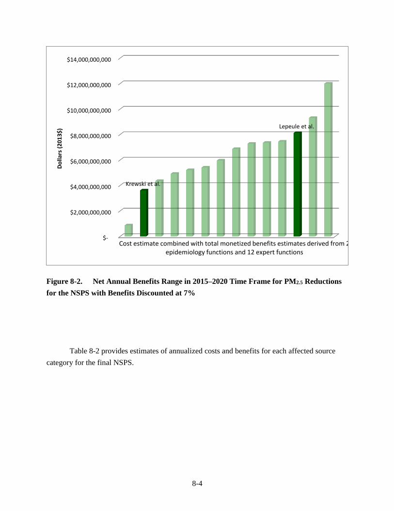
8-4
Figure 8-2. Net Annual Benefits Range in 2015–2020 Time Frame for PM2.5 Reductions
for the NSPS with Benefits Discounted at 7%
Table 8-2 provides estimates of annualized costs and benefits for each affected source
category for the final NSPS.
$-
$2,000,000,000
$4,000,000,000
$6,000,000,000
$8,000,000,000
$10,000,000,000
$12,000,000,000
$14,000,000,000
Krewski et al.
Lepeule et al.
Do
llars
(2
01
3$
)
Cost estimate combined with total monetized benefits estimates derived from 2 epidemiology functions and 12 expert functions

8-5
Table 8-2. Compliance Costs, Monetized Benefits, and Monetized Net Benefits (2013
dollars) by Source Category in the 2015–2020 Time Frame—Final NSPS
Source Category
Total Annualized
Costs
($ millions)
Monetized Benefits
($ millions)a
Monetized Net
Benefits ($ millions)
Wood stoves $3 $14 to $31
$11 to $28
Single burn rate stoves $1 $280 to $630 $280 to $630
Pellet stoves $2 $2 to $5 $0. to $3
Forced-air furnaces $15 $1,700 to $3,700 $1,700 to $3,700
Hydronic heating systems $25 $1,400 to $3,200 $1,400 to $3,200
a All estimates are an average of annual impacts for the time frame from 2015 to 2020 inclusive. All estimates are
in 2013 dollars. These results include units anticipated to come online and the lowest cost disposal assumption.
Total annualized costs are estimated at a 7% interest rate to be consistent with OMB guidance. Total annualized
costs are also estimated at a 3% interest rate for each source category to be consistent with OMB guidance, and
these costs are about 13% less than the total annualized costs presented in this table. These costs are presented in
Section 5 of this RIA and in the cost memoranda for this final rule. The monetized net benefits with total
annualized costs at a 3% interest rate are minimally different than those calculated with total annualized costs at a
7% interest rate. b Total monetized benefits are estimated at a 3% discount rate. The total monetized benefits reflect the human
health benefits associated with reducing exposure to PM2.5 through reductions of directly emitted PM2.5. It is
important to note that the monetized benefits include many but not all health effects associated with PM2.5
exposure. Benefits are shown as a range from Krewski et al. (2009) to Lepeule et al. (2012). These models assume
that all fine particles, regardless of their chemical composition, are equally potent in causing premature mortality
because the scientific evidence is not yet sufficient to allow differentiation of effect estimates by particle type.
Because these estimates were generated using benefit-per-ton estimates, we do not break down the total
monetized benefits into specific components here. See Figure 7-1 in this RIA for an illustration of the breakdown,
or the RIA for the final Cross-States Air Pollution Rule (EPA, 2011) for more information.

9-1
SECTION 9
REFERENCES AND COST APPENDIX
Abt Associates, Inc. 2012. BenMAP User’s Manual Appendices. Prepared for U.S. Environmental Protection
Agency Office of Air Quality Planning and Standards. Research Triangle Park, NC. September.
Available on the Internet at http://www.epa.gov/air/benmap/models/BenMAPAppendicesOct2012.pdf.
Agency for Toxic Substances and Disease Registry (ATSDR). 1995. Toxicological Profile for Polycyclic
Aromatic Hydrocarbons (PAHs). Atlanta, GA: U.S. Department of Health and Human Services, Public
Health Service. Available at: http://www.atsdr.cdc.gov/ToxProfiles/TP.asp?id=122&tid=25
American Enterprise Institute (AEI) and Brookings Institution Joint Center for Regulatory Studies. 1986. NSPS
for Residential Wood Heaters. Regulatory Impact Analysis. RIN: 2060-AB68. Available at: http://reg-
markets.org/admin/authorpdfs/redirect-safely.php?fname=../pdffiles/2060-AB68.RIA.pdf
Bernstein, M.A., and J. Griffin. 2005. Regional Differences in the Price-Elasticity of Demand for Energy. The
RAND Corporation. Available at: http://www.rand.org/pubs/technical_reports/2005/RAND_TR292.pdf.
Chernov, A. 2008. Masonry Heaters: Planning Guide for Architects, Home Designers, and builders.
Stovemaster Web site. Available at: http://www.stovemaster.com/files/masonry.pdf.
Dagan, D. January 7, 2005. “Warming Up to Stoves.” Central Penn Business Journal. Available at:
http://www.allbusiness.com/sales/1033217-1.html
Dun & Bradstreet (D&B). 2010. D&B Marketplace. A company information database searchable by NAICS
code. Accessed on July 15, 2010.
Fann, N., C.M. Fulcher, B.J. Hubbell. 2009. “The influence of location, source, and emission type in estimates
of the human health benefits of reducing a ton of air pollution.” Air Qual Atmos Health 2:169–176.
Fann, N., K.R. Baker, and C.M. Fulcher. 2012. “Characterizing the PM2.5-related health benefits of emission
reductions for 17 industrial, area and mobile emission sectors across the U.S.” Environment
International 49 41–151.
Gwinn, M.R., J. Craig, D.A. Axelrad, R. Cook, C. Dockins, N. Fann, R. Fegley, D.E. Guinnup, G. Helfand, B.
Hubbell, S.L. Mazur, T. Palma, R.L. Smith, J. Vandenberg, and B. Sonawane. 2011. “Meeting report:
Estimating the benefits of reducing hazardous air pollutants—summary of 2009 workshop and future
considerations.” Environ Health Perspect. Jan; 119(1): p. 125-30.
Industrial Economics, Inc (IEc). 2009. Section 812 Prospective Study of the Benefits and Costs of the Clean Air
Act: Air Toxics Case Study—Health Benefits of Benzene Reductions in Houston, 1990–2020. Final
Report, July 14, 2009. Available on the Internet at
http://www.epa.gov/air/sect812/dec09/812CAAA_Benzene_Houston_Final_Report_July_2009.pdf.
Industrial Economics, Incorporated (IEc). 2006. Expanded Expert Judgment Assessment of the Concentration-
Response Relationship Between PM2.5 Exposure and Mortality. Prepared for: Office of Air Quality
Planning and Standards, U.S. Environmental Protection Agency, Research Triangle Park, NC.
September. Available on the Internet at
http://www.epa.gov/ttn/ecas/regdata/Uncertainty/pm_ee_tsd_expert_interview_summaries.pdf.

9-2
Krewski D, Jerrett M, Burnett RT, Ma R, Hughes E, Shi, Y, et al. 2009. Extended follow-up and spatial analysis
of the American Cancer Society study linking particulate air pollution and mortality. HEI Research
Report, 140, Health Effects Institute, Boston, MA.
Lepeule J, Laden F, Dockery D, Schwartz J 2012. “Chronic Exposure to Fine Particles and Mortality: An
Extended Follow-Up of the Harvard Six Cities Study from 1974 to 2009.” Environ Health Perspect.
Jul;120(7):965-70.
National Research Council (NRC). 2002. Estimating the Public Health Benefits of Proposed Air Pollution
Regulations. Washington, DC: The National Academies Press.
Office of Management and Budget (OMB). 2003. Circular A-4: Regulatory Analysis. Washington, DC.
Available on the Internet at http://www.whitehouse.gov/omb/circulars/a004/a-4.html.
Roman, Henry A., Katherine D. Walker, Tyra L. Walsh, Lisa Conner, Harvey M. Richmond, Bryan J. Hubbell,
and Patrick L. Kinney. 2008. “Expert Judgment Assessment of the Mortality Impact of Changes in
Ambient Fine Particulate Matter in the U.S.” Environ. Sci. Technol., 42(7):2268-2274.
Sisler, J.F. 1996. Spatial and seasonal patterns and long-term variability of the composition of the haze in the
United States: an analysis of data from the IMPROVE network. CIRA Report, ISSN 0737-5352-32,
Colorado State University.
U.S. Census Bureau. 2008a. Firm Size Data from the Statistics of U.S. Businesses: U.S. Detail Employment
Sizes: 2002. <http://www2.census.gov/csd/susb/2002/ 02us_detailed%20sizes_6digitnaics.txt >
U.S. Environmental Protection Agency—Science Advisory Board (U.S. EPA-SAB). 2002. Workshop on the
Benefits of Reductions in Exposure to Hazardous Air Pollutants: Developing Best Estimates of Dose-
Response Functions An SAB Workshop Report of an EPA/SAB Workshop (Final Report). EPA-SAB-EC-
WKSHP-02-001. January. Available on the Internet at
http://yosemite.epa.gov/sab%5CSABPRODUCT.NSF/34355712EC011A358525719A005BF6F6/$File/
ecwkshp02001%2Bappa-g.pdf.
U.S. Environmental Protection Agency (U.S. EPA). 1995. Regulatory Impact Analysis for the Petroleum
Refinery NESHAP. Revised Draft for Promulgation. Office of Air Quality Planning and Standards,
Research Triangle Park, N.C. Available on the Internet at http://envinfo.com/caain/mact/petroria.html.
U.S. Environmental Protection Agency (U.S. EPA). 2006. Air Quality Criteria for Ozone and Related
Photochemical Oxidants (Final). EPA/600/R-05/004aF-cF. Washington, DC: U.S. EPA. February.
Available on the Internet at http://cfpub.epa.gov/ncea/CFM/recordisplay.cfm?deid=149923.
U.S. Environmental Protection Agency (U.S. EPA). 2008a. Integrated Science Assessment for Sulfur Oxides—
Health Criteria (Final Report). National Center for Environmental Assessment, Research Triangle Park,
NC. September. Available on the Internet at
http://cfpub.epa.gov/ncea/cfm/recordisplay.cfm?deid=198843.
U.S. Environmental Protection Agency (U.S. EPA). 2008c. Integrated Science Assessment for Oxides of
Nitrogen—Health Criteria (Final Report). National Center for Environmental Assessment, Research
Triangle Park, NC. July. Available at at http://cfpub.epa.gov/ncea/cfm/recordisplay.cfm?deid=194645.

9-3
U.S. Environmental Protection Agency (U.S. EPA). 2008d. Integrated Science Assessment for Oxides of
Nitrogen and Sulfur–Ecological Criteria National (Final Report). National Center for Environmental
Assessment, Research Triangle Park, NC. EPA/600/R-08/139. December. Available at
http://cfpub.epa.gov/ncea/cfm/recordisplay.cfm?deid=201485.
U.S. Environmental Protection Agency (U.S. EPA). 2009. Integrated Science Assessment for Particulate Matter
(Final Report). EPA-600-R-08-139F. National Center for Environmental Assessment—RTP Division.
December. Available on the Internet at http://cfpub.epa.gov/ncea/cfm/recordisplay.cfm?deid=216546.
U.S. Environmental Protection Agency (U.S. EPA). 2010a. Integrated Science Assessment for Carbon
Monoxide. National Center for Environmental Assessment, Research Triangle Park, NC. EPA/600/R-
09/019F. January. Available at http://cfpub.epa.gov/ncea/cfm/recordisplay.cfm?deid=218686.
U.S. Environmental Protection Agency (U.S. EPA). 2010b. Technical Support Document: Summary of Expert
Opinions on the Existence of a Threshold in the Concentration-Response Function for PM2.5-related
Mortality. Research Triangle Park, NC. June. Available on the Internet at
www.epa.gov/ttn/ecas/regdata/Benefits/thresholdstsd.pdf.
U.S. Environmental Protection Agency (U.S. EPA). 2010c. Valuing Mortality Risk Reductions for
Environmental Policy: A White Paper: SAB Review Draft. National Center for Environmental
Economics December. Available on the Internet at http://yosemite.epa.gov/ee/epa/eerm.nsf/vwAN/EE-
0563-1.pdf/$file/EE-0563-1.pdf.
U.S. Environmental Protection Agency (U.S. EPA). 2010e. Guidelines for Preparing Economic Analyses. EPA
240-R-10-001. National Center for Environmental Economics, Office of Policy Economics and
Innovation. Washington, DC. December. Available on the Internet at
http://yosemite.epa.gov/ee/epa/eerm.nsf/vwAN/EE-0568-50.pdf/$file/EE-0568- 50.pdf.
U.S. Environmental Protection Agency (U.S. EPA). 2011a. The Benefits and Costs of the Clean Air Act from
1990 to 2020. Office of Air and Radiation, Washington, DC. March.
http://www.epa.gov/air/sect812/feb11/fullreport.pdf. Accessed March 30, 2011.
U.S. Environmental Protection Agency (U.S. EPA). 2011b. Regulatory Impact Analysis for the Final Mercury
and Air Toxics Standards. EPA-452/R-11-011. December. Available on the Internet at
http://www.epa.gov/ttn/ecas/regdata/RIAs/matsriafinal.pdf.
U.S. Environmental Protection Agency (U.S. EPA). 2011c. 2005 National-Scale Air Toxics Assessment. Office
of Air Quality Planning and Standards, Research Triangle Park, NC. March. Available on the Internet at
http://www.epa.gov/ttn/atw/nata2005/.
U.S. Environmental Protection Agency (U.S. EPA). 2011d. Regulatory Impact Analysis: National Emission
Standards for Hazardous Air Pollutants for Industrial, Commercial, and Institutional Boilers and
Process Heaters. February. Available on the Internet at
http://www.epa.gov/ttnecas1/regdata/RIAs/boilersriafinal110221_psg.pdf.
U.S. Environmental Protection Agency (U.S. EPA). 2012a. Regulatory Impact Analysis for the Final Revisions
to the National Ambient Air Quality Standards for Particulate Matter. EPA-452/R-12-003. Office of Air
Quality Planning and Standards, Health and Environmental Impacts Division. December. Available at
http://www.epa.gov/pm/2012/finalria.pdf.
9-4
U.S. Environmental Protection Agency (U.S. EPA). 2012b. Regulatory Impact Analysis: Petroleum Refineries
New Source Performance Standards Ja. Office of Air Quality Planning and Standards, Health and
Environmental Impacts Division. June. Available at
http://www.epa.gov/ttnecas1/regdata/RIAs/refineries_nsps_ja_final_ria.pdf.
U.S. Environmental Protection Agency (U.S. EPA). 2013. Technical Support Document: Estimating the Benefit
per ton of Reducing PM2.5 Precursors from 17 sectors. Office of Air Quality Planning and Standards,
Research Triangle Park, NC. February.
U.S. Environmental Protection Agency—Science Advisory Board (U.S. EPA-SAB). 2008. Characterizing
Uncertainty in Particulate Matter Benefits Using Expert Elicitation. EPA-COUNCIL-08-002. July.
Available on the Internet at
http://yosemite.epa.gov/sab/sabproduct.nsf/0/43B91173651AED9E85257487004EA6CB/$File/EPA-
COUNCIL-08-002-unsigned.pdf.
U.S. Environmental Protection Agency—Science Advisory Board (U.S. EPA-SAB). 2000. An SAB Report on
EPA’s White Paper Valuing the Benefits of Fatal Cancer Risk Reduction. EPA-SAB-EEAC-00-013.
July. Available on the Internet at
http://yosemite.epa.gov/sab%5CSABPRODUCT.NSF/41334524148BCCD6852571A700516498/$File/e
eacf013.pdf.
U.S. Environmental Protection Agency—Science Advisory Board (U.S. EPA-SAB). 2004c. Advisory Council
on Clean Air Compliance Analysis Response to Agency Request on Cessation Lag. EPA-COUNCIL-
LTR-05-001. December. Available on the Internet at <.
http://yosemite.epa.gov/sab/sabproduct.nsf/0/39F44B098DB49F3C85257170005293E0/$File/council_lt
r_05_001.pdf
U.S. Environmental Protection Agency—Science Advisory Board (U.S. EPA-SAB). 2008. Benefits of Reducing
Benzene Emissions in Houston, 1990–2020. EPA-COUNCIL-08-001. July. Available at
http://yosemite.epa.gov/sab/sabproduct.nsf/D4D7EC9DAEDA8A548525748600728A83/$File/EPA-
COUNCIL-08-001-unsigned.pdf.
U.S. Environmental Protection Agency—Science Advisory Board (U.S. EPA-SAB). 2009b. Review of EPA’s
Integrated Science Assessment for Particulate Matter (First External Review Draft, December 2008).
EPA-COUNCIL-09-008. May. Available on the Internet at
http://yosemite.epa.gov/sab/SABPRODUCT.NSF/81e39f4c09954fcb85256ead006be86e/73ACCA834A
B44A10852575BD0064346B/$File/EPA-CASAC-09-008-unsigned.pdf.
U.S. Environmental Protection Agency—Science Advisory Board (U.S. EPA-SAB). 2009c. Review of
Integrated Science Assessment for Particulate Matter (Second External Review Draft, July 2009). EPA-
CASAC-10-001. November. Available on the Internet at
http://yosemite.epa.gov/sab/SABPRODUCT.NSF/81e39f4c09954fcb85256ead006be86e/151B1F83B02
3145585257678006836B9/$File/EPA-CASAC-10-001-unsigned.pdf.
U.S. Environmental Protection Agency—Science Advisory Board (U.S. EPA-SAB). 2010a. Review of EPA’s
DRAFT Health Benefits of the Second Section 812 Prospective Study of the Clean Air Act. EPA-
COUNCIL-10-001. June. Available on the Internet at
http://yosemite.epa.gov/sab/sabproduct.nsf/9288428b8eeea4c885257242006935a3/59e06b6c5ca665978
52575e7006c5d09!OpenDocument&TableRow=2.3#2.

9-5
U.S. Environmental Protection Agency—Science Advisory Board (U.S. EPA-SAB). 2011. Review of Valuing
Mortality Risk Reductions for Environmental Policy: A White Paper (December 10, 2010). EPA-SAB-
11-011 July. Available on the Internet at
http://yosemite.epa.gov/sab/sabproduct.nsf/298E1F50F844BC23852578DC0059A616/$File/EPA-SAB-
11-011-unsigned.pdf .
Fann, N., C. M. Fulcher, and B. J. Hubbell. 2009. “The Influence of Location, Source, and Emission Type in
Estimates of the Human Health Benefits of Reducing a Ton of Air Pollution.” Air Quality, Atmosphere,
and Health 2:169-176.
Fireplaces & Woodstoves. 2010. “Masonry Heaters.” http://www.fireplacesandwoodstoves.com/indoor-
fireplaces/masonry-fireplaces.aspx.
Frost & Sullivan. 2010. Project: Market Research and Report on North American Residential Wood Heaters,
Fireplaces, and Hearth Heating Products Market (P.O. # PO1-IMP402-F&S). Prepared for EC/R.
Fullerton, D., and G. Metcalf. 2002. “Tax Incidence.” In A. Auerbach and M. Feldstein, eds., Handbook of
Public Economics, Vol. 4, Amsterdam: Elsevier.Hearth, Patio, and Barbeque Association (HPBA).
2010a. “Comments for the Small Business Advocacy Review (SBAR) Panel, Regarding the Revision of
New Source Performance Standards for New Residential Wood Heaters.” Comments submitted to EPA
on September 12, 2010.
Gwinn, M.R., J. Craig, D.A. Axelrad, R. Cook, C. Dockins, N. Fann, R. Fegley, D.E. Guinnup, G. Helfand, B.
Hubbell, S.L. Mazur, T. Palma, R.L. Smith, J. Vandenberg, and B. Sonawane. 2011. “Meeting report:
Estimating the benefits of reducing hazardous air pollutants—summary of 2009 workshop and future
considerations.” Environ Health Perspect. 119(1): p. 125-30.
Hearth, Patio, and Barbeque Association (HPBA). 2010b. “Fireplace Insert Fact Sheet.” Available at:
http://static.hpba.org/fileadmin/factsheets/product/FS_FireplaceInsert.pdf.
Hearth, Patio, and Barbecue Association (HPBA). 2010c. “Outdoor Heating Options.” Available at:
http://www.hpba.org/consumers/outdoor-living/outdoor-heating-options.
Houck, J. 2009. “Let’s Not Forget about Coal.” Hearth & Home. December. Available at:
http://www.hearthandhome.com/articles.html.
Houck, J., and P. Tiegs. 2009. “There’s a Freight Train Comin’.” Hearth & Home. December. Available at:
http://www.hearthandhome.com/articles.html.
Industrial Economics, Inc (IEc). 2006. Expanded Expert Judgment Assessment of the Concentration-Response
Relationship Between PM2.5 Exposure and Mortality. Prepared for the U.S. EPA, Office of Air Quality
Planning and Standards, September. Available at:
http://www.epa.gov/ttn/ecas/regdata/Uncertainty/pm_ee_report.pdf.
Industrial Economics, Inc (IEc). 2009. Section 812 Prospective Study of the Benefits and Costs of the Clean Air
Act: Air Toxics Case Study—Health Benefits of Benzene Reductions in Houston, 1990–2020. Final
Report, July 14, 2009.
http://www.epa.gov/air/sect812/dec09/812CAAA+Benzene_Houston_Final_Report_July_2009.pdf.
Accessed March 30, 2011.

9-6
Kochi, I., B. Hubbell, and R. Kramer. 2006. “An Empirical Bayes Approach to Combining Estimates of the
Value of Statistical Life for Environmental Policy Analysis.” Environmental and Resource Economics
34:385-406.
Krewski D, Jerrett M, Burnett RT, Ma R, Hughes E, Shi, Y, et al. 2009. Extended follow-up and spatial analysis
of the American Cancer Society study linking particulate air pollution and mortality. HEI Research
Report, 140, Health Effects Institute, Boston, MA.
Laden, F., J. Schwartz, F.E. Speizer, and D.W. Dockery. 2006. Reduction in Fine Particulate Air Pollution and
Mortality. American Journal of Respiratory and Critical Care Medicine. 173: 667-672.
Landsburg, S.H. 2005. Price Theory and Applications. 6th Ed. Thomson South Western.Mason, OH.
Mankiw, N.G. 1998. Principles of Economics. Orlando, Fl: Dryden Press.
Masonry Heater Association of North America (MHA). 1998. MHA Masonry Heater Definition. Available at:
http://mha-net.org/docs/def-mha.htm.
Morgenstern, R. D., W. A. Pizer, and J. S. Shih. 2002. “Jobs versus the Environment: An Industry-Level
Perspective.” Journal of Environmental Economics and Management 43(3):412-436. Available at
http://ac.els-cdn.com/S009506960191191X/1-s2.0-S009506960191191X-main.pdf?_tid=6bc8845e-
7c56-11e2-84a7-00000aab0f26&acdnat=1361472319_4fe7ef315e9b2f8fc064c0a767895205
(subscription required).
Mrozek, J.R., and L.O. Taylor. 2002. “What Determines the Value of Life? A Meta-Analysis.” Journal of
Policy Analysis and Management 21(2):253-270.
National Research Council (NRC). 2002. Estimating the Public Health Benefits of Proposed Air Pollution
Regulations. Washington, DC: The National Academies Press.
Nicholson, Walter. 1998. Microeconomic Theory. Orlando: The Dryden Press.
Northeast States for Coordinated Air Use Management (NESCAUM). 2006. Assessment of Outdoor Wood-
Fired Boilers. March, 2006 (Revised June, 2006). Available at:
http://www.nescaum.org/documents/assessment-of-outdoor-wood-fired-boilers.
Office of Management and Budget (OMB). 2003. Circular A-4: Regulatory Analysis. Washington, DC.
Available on the Internet at http://www.whitehouse.gov/omb/circulars/a004/a-4.html.
Pope, C.A., III, R.T. Burnett, M.J. Thun, E.E. Calle, D. Krewski, K. Ito, and G.D. Thurston. 2002. “Lung
Cancer, Cardiopulmonary Mortality, and Long-term Exposure to Fine Particulate Air Pollution.”
Journal of the American Medical Association 287:1132-1141.
Roman, Henry A., Katherine D. Walker, Tyra L. Walsh, Lisa Conner, Harvey M. Richmond, Bryan.J. Hubbell,
and Patrick L. Kinney. 2008. “Expert Judgment Assessment of the Mortality Impact of Changes in
Ambient Fine Particulate Matter in the U.S. Environmental Science & Technology 42(7):2268-2274.
Sisler, J.F. 1996. Spatial and seasonal patterns and long-term variability of the composition of the haze in the
United States: an analysis of data from the IMPROVE network. CIRA Report, ISSN 0737-5352-32,
Colorado State University.
9-7
The Risk Management Association. 2008. Annual Statement Studies, Financial Ratio Benchmarks 2008–2009.
Risk Management Association, Philadelphia: 2008.
U.S. Census Bureau. 2007. Survey of Plant Capacity: 2006. “Table 1a. Full Capacity Utilization Rates by
Industry Fourth Quarter 2002–2006.” U.S. Census Bureau: Washington DC. Report No. MQ-C1(06).
Available at: http://www.census.gov/manufacturing/capacity/historical_data/index.html.
U.S. Census Bureau. 2009. American Community Survey: 2006–2008. Available at:
http://factfinder.census.gov/servlet/DatasetMainPageServlet?_program=ACS&submenId=&_lang+en&_
ts=. U.S. Census Bureau. 2010a. American Fact Finder. Sector 31: Annual Survey of Manufactures:
General Statistics: Statistics for Industry Groups and Industries: 2008 and 2007. Available at:
http://factfinder.census.gov. Accessed July 20, 2010.
U.S. Census Bureau. 2010b. American Fact Finder. Sector 23: EC0723SG01: Construction: Summary Series:
General Summary: Detailed Statistics for Establishments: 2007. Available at:
http://factfinder.census.gov. Accessed July 20, 2010.
U.S. Census Bureau. 2010c. American Fact Finder. Sector 42: EC0742A1: Wholesale Trade: Geographic Area
Series: Summary Statistics for the United States, States, Metro Areas, Counties, and Places: 2007.
Available at: http://factfinder.census.gov. Accessed July 20, 2010.
U.S. Census Bureau. 2010d. American Fact Finder. Sector 44: EC0744A1: Retail Trade: Geographic Area
Series: Summary Statistics for the United States, States, Metro Areas, Counties, and Places: 2007.
Available at: http://factfinder.census.gov. Accessed July 20, 2010.
U.S. Census Bureau. 2010e. Census Regions and Divisions of the United States. Available at:
http://www.census.gov/geo/www/us_regdiv.pdf. Accessed September 12, 2010.
U.S. Census Bureau. 2010f. North American Industrial Classification System [NAICS] Code Definitions Web
site. Available at: http://www.census.gov/eos/www/naics/.
U.S. Department of Energy (DOE). 2009. “Your Home: Selecting Heating Fuel and System Types.”
ENERGYSTAR Web site. U.S. Department of Energy. Available at:
http://www.energysavers.gov/your_home/space_heating_cooling/index.cfm/mytopic=12330..
U.S. Department of Energy (DOE). 2010. “Your Home: Masonry Heaters.” ENERGYSTAR Web site. U.S.
Department of Energy. Available at:
http://www.energysavers.gov/your_home/space_heating_cooling/index.cfm/mytopic=12570.
U.S. Energy Information Administration (EIA). 2011. Residential Energy Consumption Survey: 2009. Available
at: http://www.eia.doe.gov/emeu/recs/recspubuse05/pubuse05.html.
U.S. Environmental Protection Agency—Science Advisory Board (U.S. EPA-SAB). 2007. SAB Advisory on
EPA’s Issues in Valuing Mortality Risk Reduction. EPA-SAB-08-001. October. Available on the
Internet at
<http://yosemite.epa.gov/sab/sabproduct.nsf/4128007E7876B8F0852573760058A978/$File/sab-08-
001.pdf >.

9-8
U.S. Environmental Protection Agency—Science Advisory Board (U.S. EPA-SAB). 2009a. Review of EPA’s
Integrated Science Assessment for Particulate Matter (First External Review Draft, December 2008).
EPA-COUNCIL-09-008. May. Available on the Internet at
<http://yosemite.epa.gov/sab/SABPRODUCT.NSF/81e39f4c09954fcb85256ead006be86e/73ACCA834
AB44A10852575BD0064346B/$File/EPA-CASAC-09-008-unsigned.pdf>.
U.S. Environmental Protection Agency—Science Advisory Board (U.S. EPA-SAB). 2009b. Consultation on
EPA’s Particulate Matter National Ambient Air Quality Standards: Scope and Methods Plan for Health
Risk and Exposure Assessment. EPA-COUNCIL-09-009. May. Available on the Internet at
<http://yosemite.epa.gov/sab/SABPRODUCT.NSF/81e39f4c09954fcb85256ead006be86e/723FE644C5
D758DF852575BD00763A32/$File/EPA-CASAC-09-009-unsigned.pdf>.
U.S. Environmental Protection Agency—Science Advisory Board (U.S. EPA-SAB). 2010. Review of EPA’s
DRAFT Health Benefits of the Second Section 812 Prospective Study of the Clean Air Act. EPA-
COUNCIL-10-001. June. Available on the Internet at
http://yosemite.epa.gov/sab/sabproduct.nsf/0/72D4EFA39E48CDB28525774500738776/$File/EPA-
COUNCIL-10-001-unsigned.pdf.
U.S. Environmental Protection Agency (EPA). 2002. “Profile of the Pulp and Paper Industry.” Sector Notebook
Project. Available at:
http://www.epa.gov/Compliance/resources/publications/assistance/sectors/notebooks/index.html.
U.S. Environmental Protection Agency (EPA). 2006a. Final Guidance EPA Rulewriters: Regulatory Flexibility
Act as Amended by the Small Business and Regulatory Enforcement Fairness Act.
http://www.epa.gov/sbrefa/documents/rfaguidance11-00-06.pdf.
U.S. Environmental Protection Agency (EPA). 2006b. Regulatory Impact Analysis. 2006 National Ambient Air
Quality Standards for Particulate Matter. Chapter 5. Available at:
http://www.epa.gov/ttn/ecas/regdata/RIAs/Chapter%205--Benefits.pdf.
U.S. Environmental Protection Agency (EPA). 2008a. Integrated Science Assessment for Sulfur Oxides—Health
Criteria (Final Report). National Center for Environmental Assessment, Research Triangle Park, NC.
Available at: http://cfpub.epa.gov/ncea/cfm/recordisplay.cfm?deid=198843.
U.S. Environmental Protection Agency (U.S. EPA). 2008b. Integrated Science Assessment for Sulfur Oxides—
Health Criteria (Final Report). National Center for Environmental Assessment, Research Triangle Park,
NC. Available at http://cfpub.epa.gov/ncea/cfm/recordisplay.cfm?deid=198843.
U.S. Environmental Protection Agency (U.S. EPA). 2008c. Integrated Science Assessment for Oxides of
Nitrogen—Health Criteria (Final Report). National Center for Environmental Assessment, Research
Triangle Park, NC. July. Available at at http://cfpub.epa.gov/ncea/cfm/recordisplay.cfm?deid=194645.
U.S. Environmental Protection Agency (U.S. EPA). 2008d. Integrated Science Assessment for Oxides of
Nitrogen and Sulfur–Ecological Criteria National (Final Report). National Center for Environmental
Assessment, Research Triangle Park, NC. EPA/600/R-08/139. December. Available at
http://cfpub.epa.gov/ncea/cfm/recordisplay.cfm?deid=201485.
U.S. Environmental Protection Agency (U.S. EPA). 2009a. Regulatory Impact Analysis: National Emission
Standards for Hazardous Air Pollutants from the Portland Cement Manufacturing Industry. Office of
Air Quality Planning and Standards, Research Triangle Park, NC. April. Available on the Internet at
<http://www.epa.gov/ttn/ecas/regdata/RIAs/portlandcementria_4-20-09.pdf >.
9-9
U.S. Environmental Protection Agency (U.S. EPA). 2009b. Integrated Science Assessment for Particulate
Matter (Final Report). EPA-600-R-08-139F. National Center for Environmental Assessment—RTP
Division. December. Available on the Internet at
<http://cfpub.epa.gov/ncea/cfm/recordisplay.cfm?deid=216546>.
U.S. Environmental Protection Agency (EPA). 2009c. Subpart AAA-Standards of Performance for New
Residential Wood Heaters. Discussion Draft. Available at: http://www.hpba.org/admin/NSPS-Review-
Document.pdf.
U.S. Environmental Protection Agency (EPA). 2010a. Integrated Science Assessment for Carbon Monoxide.
National Center for Environmental Assessment, Research Triangle Park, NC. EPA/600/R-09/019F.
January. Available at: http://cfpub.epa.gov/ncea/cfm/recordisplay.cfm?deid=218686.
U.S. Environmental Protection Agency (EPA). 2010b. Final Regulatory Impact Analysis (RIA) for the SO2
National Ambient Air Quality Standards (NAAQS). Office of Air Quality Planning and Standards,
Research Triangle Park, NC. June. Available at:
http://www.epa.gov/ttn/ecas/regdata/RIAs/fso2ria100602full.pdf.
U.S. Environmental Protection Agency (EPA). 2010c. Guidelines for Preparing Economic Analyses. EPA 240-
R-10-001. Washington, DC: National Center for Environmental Economics, Office of Policy Economics
and Innovation. Available at: http://yosemite.epa.gov/ee/epa/eed.nsf/pages/guidelines.html.
U.S. Environmental Protection Agency (EPA). 2010d. Lowest Measured Level (LML) Assessment for Rules
without Policy-Specific Air Quality Data Available: Technical Support Document. Office of Air Quality
Planning and Standards, Research Triangle Park, NC. July. Available at:
http://www.epa.gov/ttn/ecas/regdata/Benefits/thresholdstsd.pdf.
U.S. Environmental Protection Agency (EPA). 2010e. Regulatory Impact Analysis for the Proposed Federal
Transport Rule. Office of Air Quality Planning and Standards, Research Triangle Park, NC. July.
Available at: http://www.epa.gov/ttn/ecas/regdata/RIAs/proposaltrria_final.pdf.
U.S. Environmental Protection Agency (EPA). 2010f. Regulatory Impact Analysis for the SO2 NAAQS. Office
of Air Quality Planning and Standards, Research Triangle Park, NC. June. Available at:
http://www.epa.gov/ttn/ecas/regdata/RIAs/fso2ria100602full.pdf.
U.S. Environmental Protection Agency (EPA). May 2004. Final Regulatory Analysis: Control of Emissions
from Nonroad Diesel Engines. EPA420-R-04-007. Washington, DC: EPA. http://www.epa.gov/nonroad-
diesel/2004fr/420r04007.pdf.
U.S. Environmental Protection Agency (U.S. EPA). 2010b. Technical Support Document: Summary of Expert
Opinions on the Existence of a Threshold in the Concentration-Response Function for PM2.5-related
Mortality. Research Triangle Park, NC. June. Available on the Internet at
www.epa.gov/ttn/ecas/regdata/Benefits/thresholdstsd.pdf.
U.S. Environmental Protection Agency (U.S. EPA). 2010c. Guidelines for Preparing Economic Analyses. EPA
240-R-10-001. National Center for Environmental Economics, Office of Policy Economics and
Innovation. Washington, DC. December. Available on the Internet at
<http://yosemite.epa.gov/ee/epa/eerm.nsf/vwAN/EE-0568-50.pdf/$file/EE-0568-50.pdf>.
9-10
U.S. Environmental Protection Agency (U.S. EPA). 2011a. The Benefits and Costs of the Clean Air Act from
1990 to 2020. Office of Air and Radiation, Washington, DC. March.
http://www.epa.gov/air/sect812/feb11/fullreport.pdf. Accessed March 30, 2011.
U.S. Environmental Protection Agency (U.S. EPA). 2011b. Regulatory Impact Analysis for the Final Transport
Rule. Office of Air Quality Planning and Standards, Research Triangle Park, NC. June. Available at
http://www.epa.gov/airtransport/pdfs/FinalRIA.pdf.
U.S. Environmental Protection Agency. 2006. Regulatory Impact Analysis, 2006 National Ambient Air Quality
Standards for Particulate Matter, Chapter 5. Available at
<http://www.epa.gov/ttn/ecas/regdata/RIAs/Chapter%205--Benefits.pdf >.
U.S. Environmental Protection Agency. 2008a. Regulatory Impact Analysis, 2008 National Ambient Air Quality
Standards for Ground-level Ozone, Chapter 6. Available at
<http://www.epa.gov/ttn/ecas/regdata/RIAs/6-ozoneriachapter6.pdf>.
U.S. Housing and Urban Development (HUD). 2008. American Housing Survey for the United States. Multiple
Years. Table 1A-5. Available at: http://www.census.gov/hhes/www/housing/ahs/nationaldata.html.
U.S. Small Business Administration (SBA), Office of Advocacy. May 2012. A Guide for Government
Agencies, How to Comply with the Regulatory Flexibility Act, Implementing the President’s Small
Business Agenda and Executive Order 13272. Available at
http://www.sba.gov/sites/default/files/rfaguide_0512_0.pdf.
U.S. Small Business Administration (SBA). 2013. Table of Small Business Size Standards Matched to North
American Industry Classification System Codes. Effective July 14, 2014.
http://www.sba.gov/sites/default/files/files/Size_Standards_Table(1).pdf.
Viscusi, V.K., and J.E. Aldy. 2003. “The Value of a Statistical Life: A Critical Review of Market Estimates
throughout the World.” Journal of Risk and Uncertainty 27(1):5-76.
Wade, S.H. 2003. “Price Responsiveness in the AEO2003 NEMS Residential and Commercial Buildings Sector
Models.” http://www.eia.doe.gov/oiaf/analysispaper/elasticity /pdf/buildings.pdf
Wood Heat Organization. 2010. “Fireplace Inserts: The Cure for Cold Fireplaces.” Available at:
http://www.woodheat.org/technology/inserts.htm.

9-11
APPENDIX
Documentation of Costs for Residential Wood Heaters NSPS
This appendix of the RIA documents the estimated nationwide cost impacts on manufacturers of
emission reduction options being considered for residential wood heaters as part of the New Source
Performance Standards (NSPS) review of residential wood heaters. Table A-1 presents the nationwide annual
costs for each appliance type for manufacturers under the NSPS. The number of manufacturers and models for
each appliance is included in this table. All cost estimates below are calculated using a 7% interest rate.
Table A-1. Nationwide Annual Costs to Manufacturers under the Final NSPS
(Step 1
compliance)
2015 2016 2017 2018 2019
(Step 2
compliance)
2020
2021 through
20292
Wood Stoves (R&D)3 34 125 $3,024,928 $3,024,928 $3,024,928 $3,024,928 $3,024,928 $3,024,928 $0
Pellet Stoves (R&D, R&R, cert)4,7 29 125 $1,484,192 $1,484,192 $1,484,192 $1,564,285 $1,564,285 $1,564,285 $412,963
Single Burn Rate Stoves (R&D, R&R, cert.)5, 6, 7 3 20 $1,057,518 $1,057,518 $1,057,518 $680,112 $680,112 $680,112 $66,074
$5,566,638 $5,566,638 $5,566,638 $5,269,325 $5,269,325 $5,269,325 $479,037
Forced Air Furnaces (R&D, R&R, cert.)5, 6, 7 7 50 $20,905,663 $20,905,663 $12,576,770 $12,593,240 $12,593,240 $12,593,240 $257,941
Hydronic Heaters (R&D, R&R, cert.)7,8 30 120 $24,855,398 $24,855,398 $24,855,398 $24,894,927 $24,894,927 $24,894,927 $619,059
$45,761,061 $45,761,061 $37,432,168 $37,488,168 $37,488,168 $37,488,168 $877,000
$51,327,699 $51,327,699 $42,998,805 $42,757,493 $42,757,493 $42,757,493 $1,356,037Annual Cost of the Rule
# Manufac-
turers # Models
Nationwide Annual Costs 1
QQQQ: Central Heaters
AAA: Room Heaters
NSPS Subpart Appliance Type

9-12
It should be noted that Table A-1, is based on a 7% interest rate and are in 2013 dollars ($). We also
prepared these cost estimates based on a 3% interest rate. Note also that costs vary by appliance type based on
the average number of models per manufacturer. The estimate of the number of model types are described in
the unit cost memo.135 For numbers of manufacturers, we started with HPBA data, modified based on internet
searches of manufacturers of the major appliance types. 136
The total nationwide cost of the rule from years 2015 through 2020 differ based on the underlying cost
and implementation assumptions described in this memo, and are summarized below in Table A-2. Annualized
costs in Table A-2 are estimated based on a 7% interest rate.
Table A-2. Nationwide Annual Costs for 2015-2020
Year Cost under Final Rule
(2013$)
2015 51,327,699
2016 51,327,699
2017 42,998,805
2018 42,757,493
2019 42,757,493
2020 42,757,493
Finally, Table A-3 provides annual costs and emissions, and emission reductions respectively, for each
year included in the analyses, including impacts of the rule beyond 2020, and cumulative impacts.
135 Memo to Gil Wood, USEPA, from Jill Mozier, EC/R, Inc. Unit Cost Estimates of Residential Wood Heating Appliances.
November 10, 2014. 136 HPBA Solid Fuel Product List. Attachment to E-mail from John Crouch, HBPS, to Gil Wood, EPA. September 24, 2010.

9-13
Table A-3. Cost Effectiveness (CE) Based on Annual and Cumulative PM2.5 Emissions from Central Heaters (Hydronic
Heaters and Forced Air Furnaces) and Room Heaters (Wood Stoves, Pellet Stoves, and Single Burn Rate Stoves)

9-14
Baseline PM2.5
Emissions2
(tons)
NSPS PM2.5
Emissions2
(tons)
Emission
Reduction
(tons)6
CE based on
nationwide
average
annual cost
(per ton)
Baseline PM2.5
Emissions
(tons)
NSPS PM2.5
Emissions
(tons)
Emission
Reduction
(tons)6
2015 4 $51,327,699 $19,075,401 12,120 8,075 4,046 $4,715 12,120 8,075 4,046
2016 4 $51,327,699 $19,075,401 12,484 6,970 5,514 $3,459 24,604 15,044 9,560
2017 4 $42,998,805 $19,075,401 12,858 3,016 9,842 $1,938 37,462 18,061 19,402
2018 $42,757,493 $19,075,401 13,252 3,114 10,137 $1,882 50,714 21,175 29,539
2019 $42,757,493 $19,075,401 13,649 3,208 10,441 $1,827 64,363 24,383 39,980
2020 4 $42,757,493 $19,075,401 14,059 819 13,239 $1,441 78,421 25,202 53,219
2021 $1,356,037 $19,075,401 14,480 844 13,636 $1,399 92,902 26,046 66,855
2022 $1,356,037 $19,075,401 14,915 869 14,045 $1,358 107,817 26,916 80,901
2023 $1,356,037 $19,075,401 15,362 895 14,467 $1,319 123,179 27,811 95,367
2024 $1,356,037 $19,075,401 15,823 922 14,901 $1,280 139,002 28,734 110,268
2025 $1,356,037 $19,075,401 16,298 950 15,348 $1,243 155,299 29,683 125,616
2026 $1,356,037 $19,075,401 16,787 978 15,808 $1,207 172,086 30,662 141,424
2027 $1,356,037 $19,075,401 17,290 1,008 16,282 $1,172 189,376 31,670 157,707
2028 $1,356,037 $19,075,401 17,809 1,038 16,771 $1,137 207,185 32,708 174,477
2029 $1,356,037 $19,075,401 18,343 1,069 17,274 $1,104 225,529 33,777 191,751
2030 225,529 33,777 191,751
2031 225,529 33,777 191,751
2032 225,529 33,777 191,751
2033 225,529 33,777 191,751
2034 225,529 33,777 191,751
2035 213,408 25,703 187,706
2036 200,925 18,733 182,192
2037 188,066 15,716 172,350
2038 174,815 12,602 162,213
2039 161,166 9,394 151,772
2040 147,107 8,575 138,532
2041 132,627 7,731 124,896
2042 117,712 6,861 110,851
2043 102,350 5,966 96,384
2044 86,527 5,043 81,483
2045 70,229 4,094 66,136
2046 53,442 3,115 50,327
2047 3 36,152 2,107 34,045
2048 3 18,343 1,069 17,274
$286,131,014 2,726,669 $105
6 In order to not overstate emission reductions caused by the NSPS, emissions are reduced to discount room heaters and central heaters already meeting the Step 2 limit
(i.e., 26% of wood stoves, 70% of pellet stoves and 18% of hydronic heaters are estimated to already meet the Step 2 limit).
Table A-24. Cost Effectiveness (CE) based on annual and cumulative PM2.5 emissions from Central Heaters (Forced Air Furnaces and Hydronic Heating Systems) and Room
Heaters (Wood Stoves, Pellet Stoves, and Single Burn Rate Stoves)
CE based on total
cost & cumulative
emission reduction
over 20-year
emitting lifespan
(per ton)
Emission Reduction, cumulative per year
Nationwide cumulative
cost5
Cumulative Emission
Reduction over 20-year
emitting lifespan
5 The nationwide cumulative cost represents the cost to manufacturers resulting from the R&D re-design to meet the NSPS and the NSPS-caused certification and
reporting & recordkeeping costs to bring these heaters to market from 2014 through 2029.
Year 3Nationwide
Annual Cost1
Nationwide
Average
Annual Cost
Annual Snapshots
1 Estimated nationwide annual costs are in 2013 $ and are based on a 6-year amortization period of R&D costs at a 7% interest rate (during 2015-2020), plus annual
certification and reporting & recordkeeping costs (ongoing through 2029, representing a 10 year model life). Years 2030 through 2048 are past the 10-year model design
lifespan used in this analysis.
2 Except for adjustments in years 2012 and 2018 based on an industry projections (NERA), estimated annual emissions are based on a forecasted revenue growth rate (as a
surrogate for shipments) of 3% from 2015 through 2029, for the purposes of a sensitivity analysis.
3 These heaters have in-home emitting lifespans of at least 20 years; thus models shipped in 2029 will be emitting through 2048. 4 Estimated emissions assume Step 1 standard becomes effective in 2015 and Step 2 standard in 2020 for all appliances, except forced-air furnaces have work
practice/operational standards in 2015, Step 1 emission limits for small furnaces in 2016, Step 1 emission limits for large furnaces in 2017 and Step 2 emission limits for all
furnaces in 2020.
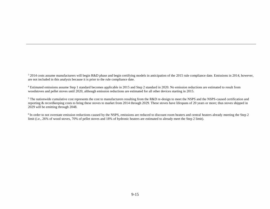
9-15
3 2014 costs assume manufacturers will begin R&D phase and begin certifying models in anticipation of the 2015 rule compliance date. Emissions in 2014, however,
are not included in this analysis because it is prior to the rule compliance date.
4 Estimated emissions assume Step 1 standard becomes applicable in 2015 and Step 2 standard in 2020. No emission reductions are estimated to result from
woodstoves and pellet stoves until 2020, although emission reductions are estimated for all other devices starting in 2015.
5 The nationwide cumulative cost represents the cost to manufacturers resulting from the R&D re-design to meet the NSPS and the NSPS-caused certification and
reporting & recordkeeping costs to bring these stoves to market from 2014 through 2029. These stoves have lifespans of 20 years or more; thus stoves shipped in
2029 will be emitting through 2048.
6 In order to not overstate emission reductions caused by the NSPS, emissions are reduced to discount room heaters and central heaters already meeting the Step 2
limit (i.e., 26% of wood stoves, 70% of pellet stoves and 18% of hydronic heaters are estimated to already meet the Step 2 limit).

9-16
9-17
United States
Environmental Protection
Agency
Office of Air Quality Planning and Standards
Health and Environmental Impacts Division
Research Triangle Park, NC
EPA-452/R-15-001
February, 2015