Regulations of Agricultural Markets and Economic

Performance: Evidence from Indian States

A thesis submitted to the University of Manchester for the degree of Doctor of Philosophy in the Faculty of Humanities

2013

Purnima Purohit

School of Environment and Development Institute for Development Policy and Management

2

ABSTRACT Regulations of Agricultural Markets and Economic Performance: Evidence from

Indian States

The thesis investigates the impact of a very specific state-led legislative institution of colonial lineage – the Agricultural Produce Markets Commission (APMC) Act & Rules – on uneven agricultural growth productivity and poverty outcomes across select fourteen Indian states over the post-independence period. It also studies political economy determinants of the APMC Act. This research offers the first most comprehensive empirical characterisation of agricultural marketing laws for the agriculture produce sector of the Indian economy. The thesis presents three substantive research outcomes. The first empirical chapter provides the construction of a composite multidimensional de jure time-varying index of the APMC Act & Rules for each state. The quantitative measure reveals the extent of variation in the form & trends of statutory clauses in the selected 14 Indian states from 1970-2008. Based on empirical analysis of nearly forty years of the regulatory framework of agricultural markets, the second empirical chapter demonstrates that variation in institutional market arrangements explain the marked differences in the use of modern farm inputs and growth patterns in agricultural productivity as well as rural poverty outcomes in the states of India. The results from 14 states show that states with improved regulatory arrangements in the agricultural markets have higher agricultural investment, productivity and fall in poverty. A difference of each one unit improvement in market regulations in a state is found to be associated with about 0.24 units average increase in the mean of agricultural yield productivity and an about 6.2 units average direct reduction in the mean of poverty incidence. Finally, the third chapter demonstrates presence of political economy activity in shaping of the differing APMC Act & Rules in Indian states. It suggests that ignoring potential influence of political economy factors in determining APMC Act can undermine the prospects of achieving desired policy objectives and may lead to miscalculated policy judgments. What the evidence in this thesis illustrates is that regulations matter in channelizing markets for efficiency effect on agricultural productivity and poverty reduction. It reveals that the APMC measure needs to be understood as a part of a wider political economy regulatory system and it cannot be viewed as a neutral tool which can be applied to produce predictable and consistent economic results. Agriculture growth and poverty reduction efforts would get a serious setback in states where effective institutional regulatory support was not provided as this assures vibrant market and remunerative price to farmers. The thesis’s fundamental finding is that efficient regulations encourage agricultural development which implies that any solution that looks to optimise the mechanisms around agricultural markets demands efficient and progressive evolution of the existing regulatory framework of the APMC Act. This challenges recent calls for complete dismantling of regulated markets, expressed by critics who view the current APMC Act as one of the main bottlenecks to managing food inflation and the national food security challenges in India. Given the heterogeneity of agrarian contexts, food systems and marketing dynamics being faced by the Indian farming community, well-regulated agricultural markets cannot be undermined for effective functioning of the domestic agricultural trade and development of farming community.

3

ACKNOWLEDGEMENTS

I would like to express my deep gratitude to my supervisors: Kunal Sen and Katsushi Imai for their guidance, invaluable support and constant motivation throughout the period of my researching and writing of this thesis. They have always generously found the time and patience to watch over its progress. It is for their untiring efforts, care and scholarly guidance that I could complete this thesis successfully. I would also like to thank my examiners: Sambit Bhattacharyya, University of Sussex and Adam Ozanne, University of Manchester for their constructive discussion and helpful comments on my thesis during my oral examination. The National Institute of Agricultural Marketing (NIAM), Government of India, Ministry of Agriculture, Jaipur, was much needed base for my field research and information collection. I owe thanks to Anurag Bhatnagar, Former Director General; R.P. Meena, the current Director General; Kamal Mathur, Director- Training; M.S Jairath, Director-Research, and other faculty members of NIAM for providing an intellectually stimulating and hospitable environment during my fieldwork in India. NIAM’s library was a great source of research information and data. My special thanks to M.S Jairath for sharing his invaluable knowledge, facilitating my research by providing important contacts that eased up the process of data collection from the library at the Directorate of Economics and Statistics, Ministry of Agriculture, New Delhi. I am also highly indebted to S.C. Khurana, Deputy Agricultural Marketing Adviser, for helpful discussions and his generous help in collecting of data from the library of the Directorate of Agricultural Marketing and Inspection (DMI), Ministry of Agriculture, Faridabad, Haryana. I would like to express my sincere thanks to S. Mahindra Dev, Director, Indira Gandhi Institute of Development Research (IGIDR), Mumbai, for stimulating discussions and reflections drawn from his experience. I am deeply grateful to Raghav Gaiha, University of Delhi, Amaresh Dubey, Jawaharlal Nehru University, Prema-Chandra Athukorala, Australian National University; Sukhpal Singh, Indian Institute of Management, Ahmedabad, B.K Pati, NIAM; L Rai, DMI, New Delhi and Malleswara Rao, DMI, Jaipur, for helpful discussions on my work. I am grateful for helpful comments and suggestions received at the European School on New Institutional Economics (ESNIE), France, in 2010 when this research also won the best PhD research project award. I am also thankful to Barbara Harriss-White for sharing articles on the topic and contacts of her students who were working on agricultural markets at the University of Oxford, UK. It is impossible to acknowledge individually my sense of gratefulness to the scores of individuals – my colleagues and contacts; my sister’s colleagues in her office: Indian Institute of Health Management and Research (IIHMR), Jaipur, and their contacts; NIAM’s network – who helped me to get hold of laws –APMC Act & Rules – of various states of India. The process was not easy at all and some who helped in the process have never met me; in spite of that it was done, making my research possible. My deepest thanks are due to all of them. Thanks are due to Pradeep S. Mehta, Secretary General and Bipul Chatterjee, Director, CUTS International, Jaipur, who have always been most generous in extending

4

guidance, support and opportunities that helped to shape my interest in policy research from the time I joined CUTS as a fresh graduate. Associating with CUTS during my data collection phase was more like home coming. CUTS provided me base during my field research in New Delhi. I am also grateful to Siddhartha Mitra, Former Research Director at CUTS International for his encouragement, guidance and support for my professional growth. I wish to thank all my research colleagues in IDPM and Department of Economics, University of Manchester, UK, for general discussions that helped me in my PhD study. Parts of my work were read by Christopher Foster, Carol Brunt, Samuel Hayes, Gemma Sou and my sister to check the clarity of my writing style. My sincere thanks are due to all of them. I owe special thanks to my fellow researcher and friend Gordon Abekah-Nkrumah for very fruitful discussions on econometrics on a regular basis. I would like to express my gratefulness for the generous support of the Commonwealth Scholarship that enabled me to complete my PhD research at the University of Manchester, UK. My deepest thanks are to the Institute for Development Policy and Management (IDPM), University of Manchester for sponsoring my field work in India and providing a supportive research environment throughout my research work at the University of Manchester.

The acknowledgements would not be complete without thanking to some very special people. Howard Nicholas and Arjun Bedi of International Institute of Social Studies, Netherlands, were my teachers and supervisory team during my masters’ study. Their excellent teaching helped to spark my intellectual interest to initiate this doctoral programme. And, I take this opportunity to express my heartfelt thanks to them. My dear friends, the way I address them – Chris, Gordon, Felix, Kasia, Marta, Miska, Nutch, Ob, Richa & Dhruv and Shamel – who were always around throughout the period of my study and made my PhD life surprisingly enjoyable! The love of my parents, sister, brother and his family, which was always there, was of special importance because it had nothing to do with whether I had done this PhD or not. And finally, the thesis is dedicated to my sister for her brutal honesty on my work and providing me that all-encompassing strength and support which I cannot express in words.

Manchester, UK September 2013

5

DECLARATION

No portion of the work referred to in the thesis has been submitted in support of an application for another degree or qualification of this or any other university or other institute of learning

COPYRIGHT STATEMENT

i The author of this thesis (including any appendices and/or schedules to this thesis) owns certain copyright or related rights in it (the “Copyright”) and s/he has given The University of Manchester certain rights to use such Copyright including for administrative purposes.

ii Copies of this thesis, either in full or in extracts and whether in hard or

electronic copy, may be made only in accordance with the Copyright, Designs and Patents Act 1988 (as amended) and regulations issued under it or, where appropriate, in accordance with licensing agreements which the University has from time to time. This page must form part of any such copies made.

iii The ownership of certain Copyright, patents, designs, trade marks and any

other intellectual property (the “Intellectual Property”) and any reproductions of copyright works in the thesis, for example graphs and tables (“Reproductions”), which may be described in this thesis, may not be owned by the author and may be owned by third parties. Such Intellectual Property and Reproductions cannot and must not be made available for use without the prior written permission of the owner(s) of the relevant Intellectual Property Rights and/or Reproductions.

iv. Further information on the conditions under which disclosure, publication and

commercialisation of this thesis, the Copyright and any Intellectual Property and/or Reproductions described in it may take place is available in the University IP Policy (see http://documents.manchester.ac.uk/DocuInfo.aspx?DocID=487), in any relevant Thesis restriction declarations deposited in the University Library, The University Library’s regulations (see http://www.manchester.ac.uk/library/aboutus/regulations) and in The University’s policy on Presentation of Theses.

6

Contents

1 Introduction ..................................................................................................................................... 10

2 Economic Performance of Indian Agriculture and Legal Framework for

Regulation of Agricultural Produce Markets: An Overview ............................................ 16

2.1 Significance of Agriculture, Agricultural Marketing and Regulations

of the Agricultural Produce Markets ........................................................................ 16

2.2 Legal and Administrative Framework for Regulation of Agricultural

Produce Markets in Indian states: The Genesis ....................................................... 23

2.3 Present Situation: Regulation of Agricultural Produce Markets ...................... 27

2.4 Annex .................................................................................................................... 30

3 Measurement of Regulations of the Agricultural Produce Markets: An

Application to Indian States ............................................................................................................. 31

3.1 Introduction ......................................................................................................... 32

3.2 Disputed Issues and Choices: Measurement Literature ................................... 36

3.3 The Meaning and Measurement Issues of the APMC Act and Rules ................ 39

3.4 Reading the Law: Background for Data Classification ...................................... 49

3.5 Variables ............................................................................................................... 57

3.6 Construction of Sub-indices ................................................................................ 71

3.7 Composite APMC Index Construction ................................................................ 84

3.8 The APMC Index 1970-2008: Results ................................................................ 86

3.9 Conclusion .......................................................................................................... 102

3.10 Annex ................................................................................................................ 105

4 Do Agricultural Marketing Laws Matter for Rural Growth in India? Evidence

from Indian States ................................................................................................................................ 116

4.1 Introduction ....................................................................................................... 116

4.2 Why should Legal Framework Regulating the Agricultural Markets

Matter for Economic Performance of Agriculture Sector? Conceptual

Literature .................................................................................................................. 118

4.3 Theory and Choice of Statistical Model Framework ....................................... 121

4.4 Empirical Analysis ............................................................................................. 126

4.5 The Data .............................................................................................................. 138

4.6 Econometric Results .......................................................................................... 144

7

4.7 Robustness and Alternative Model Specification ............................................ 158

4.8 APMC Measures and Poverty Reduction in Indian States .............................. 168

4.9 Data and Empirical Strategy ............................................................................. 171

4.10 Empirical Results ............................................................................................. 174

4.11 Conclusion ........................................................................................................ 180

4.12 Annex ................................................................................................................ 182

5 The Political Economy of Agricultural Marketing Laws: Evidence from the

Indian States ............................................................................................................................................ 196

5.1 Introduction ....................................................................................................... 196

5.2 APMC Act and Agricultural Produce Sector: Political Economy

Debate ....................................................................................................................... 200

5.3 The Determinants of the APMC Act: Literature............................................... 205

5.4 Econometric Specification and Methodology .................................................. 216

5.5 Data and Variables ............................................................................................. 217

5.6 Results and Discussion: The Determinants of Measures of the APMC

Act ............................................................................................................................. 224

5.7 Concluding Remarks .......................................................................................... 231

5.8 Annex .................................................................................................................. 234

6 Conclusion ....................................................................................................................................... 242

6.1 Summary of the Findings .................................................................................. 243

6.2 Relevance, Contribution and Limitation .......................................................... 247

6.3 Further Research ............................................................................................... 249

7 References ....................................................................................................................................... 253

Words: 82,281

8

LIST OF TABLES

Table 2.1: Share of Agriculture in GDP and Employment in Indian States ........................ 17 Table 2.2: Growth Rates of National State Domestic Product (NSDP) from Agriculture/hectare (States Ranked by % of Rainfed Area, lowest first)........................... 19 Table 2.3: Growth Rates of National State Domestic Product (NSDP) from Agriculture (rural) per person at 1980-81 prices ................................................................................................ 20 Table 3.1: Agricultural Produce Market (Regulation) Acts in force in (select) different states of India .............................................................................................................................................. 52 Table 3.2: Factor scores or weights, Eigenvalues and Cumulative variance from First Principle component entering the computation of the Sub-indices: Tetrachoric and Standard PCA .............................................................................................................................................. 81 Table 3.3: Correlation Table of APMC Index and sub-indices ................................................. 83 Table 3.4: Correlation Table of APMC Index (computed by three methods) .................... 86 Table 3.5: Summary Statistics of the Sub-indices and APMC Index, 1970-2008 ............. 88 Table 3.6: State-wise Summary Statistics (Mean and Std.Dev) of the Sub-indices and APMC Index ................................................................................................................................................. 92 Table 4.1: Summary Statistics, main variables ............................................................................ 141 Table 4.2: Use of Fertilizer, kg per hectare, 1970-2008 .......................................................... 145 Table 4.3: Proportion of Land Irrigated, 1970-2008 ................................................................ 145 Table 4.4: % Area under HVY Rice, 1984-2006 .......................................................................... 146 Table 4.5: % Area under HVY Wheat, 1984-2006 ...................................................................... 146 Table 4.6: Yield Productivity explained by APMC Act and Other Controls, 1970-2008: Results ......................................................................................................................................................... 150 Table 4.7: Wheat Yield Productivity explained by APMC Act and Other Controls, 1970-2008: Results ............................................................................................................................................ 154 Table 4.8: Rice Yield Productivity explained by APMC Act and Other Controls, 1970-2008:Results ............................................................................................................................................. 155 Table 4.9: Yield Productivity explained by Sub-components: Extended model, 1970-2008, FGLS ................................................................................................................................................. 159 Table 4.10: Instrumental Variable Estimation: Yield Productivity explained by APMC Act, 1970-2008 – Second Stage: IV Yield Productivity ............................................................. 167 Table 4.11: Summary Statistics: Poverty Measures, APMC measure and other control variables...................................................................................................................................................... 172 Table 4.12: Direct Effect, APMC measure and Poverty Reduction, 1970-1998 ............. 175 Table: 4.13 Direct and Indirect Effect, APMC measure and Poverty Reduction, 1970-1998 .............................................................................................................................................................. 175 Table 5.1a: Summary Statistics, 1970-2008 (Dependent Variable) ................................... 219 Table 5.1b: Summary Statistics, 1970-2008 (Independent Variables) ............................. 220 Table 5.2: State-wise Summary of Main Variables .................................................................... 223 Table 5.3: Main Results- Political Economy Determinants of the APMC Act .................. 226 Table 5.4: Political Economy Determinants: Six Sub-Indices of the APMC Act .............. 241

9

LIST OF BOXES

Box 1.1: Research Aim and Objectives of the Thesis ................................................................... 14 Box 3.1: Schema – Approach to Selection of Dimensions and Variables ............................ 45 Box 3.2: A Case of Political Activity behind APMC Act: Madhya Pradesh and Bihar ...... 93 Box 4.1: Major Rice and Wheat Producing States of India ...................................................... 148

LIST OF FIGURES

Figure 2.1: Growth Rates: GDP (overall) and GDP (Agriculture & Allied Sectors) ......... 18 Figure 2.2: Comparative Performance of Growth of GDP and Agri-GDP ............................ 21 Figure 2.3: Average Annual Growth Rate (%) of Gross State Domestic Product from Agriculture & Allied Sector, 1994-95 to 1999-2000 ................................................................... 22 Figure 3.1: APMC Composite Index by State .................................................................................. 90 Figure 3.2: Market Structure dimension of the APMC Index by State.................................. 95 Figure 3.3: Sales & Trading dimension of the APMC Index by State ..................................... 95 Figure 3.4: Market Infrastructure dimension of the APMC Index by State ........................ 96 Figure 3.5: Pro-Poor Regulatory dimension of the APMC Index by State .......................... 98 Figure 3.6: Scope of Regulated markets dimension of the APMC Index by State ............ 99 Figure 3.7: Alternative Market Channels dimension of the APMC Index by State ........ 101 Figure 4.1:State-wise Trend plots of Regulatory Measure and Agricultural Yields ..... 143

10

Chapter 1

1 Introduction

In his acceptance speech for the 1979 Nobel Prize in Economics, Theodore Schultz

observes:

“Most of the people in the world are poor, so if we knew the economics of being poor

we would know much of the economics that really matters. Most of the world's poor

people earn their living from agriculture, so if we knew the economics of agriculture we

would know much of the economics of being poor” (Shultz, 1979).

Three decades on since that prize lecture what has been learned and observed about

the economics of agriculture appears curiously paradoxical. People especially in

developing and least developing countries who depend on agriculture for their

livelihood are typically much poorer than people who work outside the agriculture

sector of an economy. They continue to represent a significant share, often the

majority, of the total number of poor people in the countries where they live. As the

general trend, productivity growth in the agricultural sector is low and less steady than

observed in other sectors of an economy. The agriculture sector’s potential on

reducing poverty contributes less in developing economies which has had traditionally

provided a good route out of poverty and formed the basis for the concurrent

industrial economic growth for a number of developed industrialised economies

(Johnston & Mellor, 1961; Hayami & Ruttan, 1970; Barrett et al., 2010).

India is one prominent case where almost three-fifths of the country’s workforce relies

on agriculture for its livelihood (Eleventh Five Year Plan 2007-2012, Planning

Commission, Government of India, 2008). However, the share of agriculture in the

country’s gross domestic product (GDP) is just one-fifth of the total (Ibid). With rapid

economic growth, agricultural growth has not responded to the accelerating income

Received 2010 Accessit Award of the Best Research Project, The European School on New Institutional Economics (ESNIE), Cargèse, France.

11

growth, and farm incomes visibly fell behind incomes earned in the rest of the

economy. Eighty percent of below poverty line families in India are rural, comprising

mainly tribal, small & marginal farmers and landless labour. Extremely wide differences

in agricultural productivity exist within the country and across the states. The lag in the

rate of productivity growth in agriculture across states and regions pose a serious

constraint on overall economic growth in the country (Ibid).

Among those concerned with performance of Indian agriculture, the unease is not

about a missing growth in the agriculture sector. The uneven performance of

agriculture, however, across the states is perplexing in its tendency for volatility and

regional growth disparity. Indian agriculture recorded high productivity growth and has

shown remarkable measures of socio-economic change in rural areas due to a

combination of policy changes, high rates of public investment in agricultural research

and new technology, supporting output prices, a regime of subsidised input prices,

infrastructure development, and so on (Ray, 2007:9). The beneficiaries of growth

productivity though were confined largely to a few states, and the poor states have

lagged behind. There is serious policy concern that the growth trends in the agriculture

sector are not uniform across states (Bajpai & Sachs, 1996; Purfield, 2006).

Furthermore, despite remarkable agricultural development, growth in Indian

agriculture has remained largely lopsided, lacking resilience. For instance, agricultural

growth in India started to slowdown in the 1990s. It decelerated from 3.5 percent

during 1981-97 to 2 percent during 1997-2005. There has been some revival in

agriculture from 2005 onwards. Agricultural growth was more than 4 percent during

2003-04 to 2007-08. At the current stage of India’s development, ensuring sustained

and inclusive growth of agriculture sector has been stated as one of the biggest

challenges for the country (Eleventh Five Year Plan 2007-2012, Planning Commission,

Government of India, 2008). Economists, using variety of tools and approaches, are

attempting to understand the relative importance of the sources of productivity

growth or productivity differences, explaining why such growth, as it occurs in the

agriculture sector remains cyclical and not linear. Thus, there is still a lack of

knowledge and clear policy advice as to what the government ought to do to promote

steady growth in agriculture productivity.

12

Since mid 1990s, debate has intensified on what explains the growth in agricultural

productivity which might occur by public support of agricultural factors to farming

community can rarely sustain and fail to transform the structure of the economy

through a process of long-term social or economic change. The key question is why

does growth, such as it takes place, remains fragile and short-lived? (Timmer, 1995;

Tomlinson, 1995; Binswanger & Deininger, 1997; Harriss et al., 2003; Dorward et al.,

2004; Rozelle & Swinnen, 2004). A consensus seems to have emerged agreeing that

the most important factor for sustained growth in agricultural productivity is the

‘nature of incentives offered to agricultural producers’ in agricultural markets (Bates,

1984:2; Schultz, 1976). Thus, the starting proposition in this research emerges from

this well-documented institutional conception. If the basic problem is failure to provide

proper incentives to farmers for raising agricultural productivity, then it follows that a

principal source of the problem in agricultural markets lies in its institutional

framework administered by the state, which determines returns to cultivators for their

produce in the markets (Bates, 1984; North, 1990). Following institutional historians, it

is assumed that an ineffective framework for regulations of agricultural marketing

system fail to provide outlets and revenue incentives for increased production. It, then,

might undercut the productive potential of the farming population and thus, shape the

nature of the growth process of agriculture in Indian states (Schultz, 1978a; Bates,

1984; North, 1990).

Today, most agricultural markets in India function under the framework of regulations

that evolved over the last sixty years, from a colonial state administrative and

regulatory structure to a later independent Indian state one. The question of poor

performance of regulatory institution of agricultural markets in the Indian states so far

is an increasingly complex and central question in the political economy of country’s

development in terms of its limited success in providing transparent marketing

practices, impersonal transaction norms, needs-based amenities and services, and an

environment conducive to growth-enhancing marketing (Expert Committee Report on

Agricultural Marketing Reforms, 2001; Shiva, 2007; Pal et al., 2008; Gopalkrishnan &

Sreenivasa, 2009; Gujral et al., 2011; Minten et al.,2012).

Additionally, a series of research studies of the political economy of agricultural

policies have highlighted the presence of political economy factors influencing the

13

institutional framework. These studies highlight that the economic institutions of food

markets are often skewed by the influential interest groups in their favour. This tends

to undermine the prospects of achieving policy objectives, introducing distortions, and

in turn, the efficiency of the market and agricultural sector (Bates, 1981; Mooij, 1998;

Harriss-White, 2005).

With a view to locating agriculture growth needs in a broader policy package, critical

question of non-functionality or even relevance of regulated agricultural markets at

the current stage of India’s development is receiving prominence. In response to the

criticism of existing problems in the regulated marketing system, states in India are

adopting varying policy approaches to improve the functioning of their agricultural

markets. Among others, it includes liberalising the agricultural market through repeal

or dismantling of the market regulations all together along with governing structure of

the agricultural markets in order to revive growth in the agricultural sector.

Hence, such implemented policy facts in the Indian states raise the obvious question: Is

inefficient functioning of agricultural markets or state neglect a sufficient ground to

recommend withdrawn of regulations by the state? It is unclear whether or not growth

and welfare will be improved either by reforming or repealing such regulations without

first analysing the growth and welfare implications of the existing regulatory laws of

the agricultural markets (Shaffer, 1979: 722). A clear understanding of existing events

and processes is the prerequisite to frame future strategic action plans to lead the

agriculture sector out of the present ‘confusion’ and ‘despair’ towards socio-economic

development of states of India ( Raul, 2001).

Events such as regional imbalances in agricultural production, high seasonality in

market arrivals and mass poverty are still the reality in India (Pal et al., 1990; Harriss-

White, 1995). It is important to recognise that if there is no clear diagnostic evaluation

of how existing rules frame, function and of the impact they have on agricultural

performance, effective evidence based policy development may not be possible and

‘anecdotal’ policy making may even lead to flawed conclusions (Cullinan 1999).

For these reasons, the aim of this thesis is to investigate whether the regulatory

institution plays a determining role in uneven economic growth in the agriculture

sector of Indian states? Does it have implications for poverty outcomes? And if so, why

does the agricultural market institution over time impact agricultural growth and

14

poverty reduction differently? Is the impact to do with the ‘form’ of the regulatory

institution and if so, why is the ‘form’ of institution so different in the different states.

What explains the emergence of such specific form of institution?

The thesis explores this enquiry through the study of a very specific regulatory

institution – the Agricultural Produce Markets Commission Act (APMC Act) – in 14

states of India for the period 1970-2008.1 As a regulatory institution, the APMC Act

evolved from a colonial administrative structure to a nationalised state one. The APMC

Act is the first exclusive statute on regulation of marketing of agricultural produce in

India whose history dates back to year 1886, when elements of regulation were first

introduced in the cotton market under the British rule.

With the above proposition, Box 1.1 sums-up the overarching research aim and

objectives of this research. The purpose of this research is to demonstrate how

variation in de jure detail of regulatory arrangements of agricultural markets has

consequences for regional lagged differences in sectoral growth and rural poverty

outcomes. By exploring political economy determinants of regulatory arrangements of

agricultural markets in Indian states, it seeks to reveal that institutional solutions to

current market problems in India are unlikely to result in predicted outcomes, if the

regulatory institution depends, to a large extent, on preference and influence of the

relevant interest groups.

Box 1.1: Research Aim and Objectives of the Thesis

1 In particular the states considered for the analysis are: Andhra Pradesh, Assam, Bihar, Gujarat, Haryana, Karnataka, Madhya Pradesh, Maharashtra, Orissa, Punjab, Rajasthan, Tamil Nadu, Uttar Pradesh and West Bengal. Together they represent around 95% of Indian population

Research Aim: To describe and explain differences in regulatory arrangements of agricultural markets and their causal linkage with economic performance of the agriculture sector. Research Objective 1: Describe and construct quantitative index measuring regulations of the agricultural markets in Indian states over the time. Research Objective 2: Empirically examine impact of regulations of agricultural markets on agricultural growth and poverty outcomes. Research Objective 3: Empirically determine and explain emergence of the specific form of regulations of the agricultural markets in Indian states.

15

This work is important because it is the first comprehensive empirical study of its kind

for the agricultural produce sector of the Indian economy. The research findings

contribute to an understanding of the effects of the legal framework for regulatory

institutions on economic performance of the agriculture sector in India. No

comprehensive empirical study has been undertaken on the ‘form’ and ‘trend’ of

regulatory legal framework within which agricultural produce marketing system of the

Indian states is structured for a period of 38 years.

The thesis is organised as follows. The next chapter provides an overview of India’s

present state of agriculture, agricultural markets, historical perspective on market

regulations and India’s economic policy challenges. Chapter three presents state-wise

quantitative measurement of the Agricultural Produce Markets Commission (APMC)

Act & Rules of post-harvest agricultural markets for major 14 states of India over the

time 1970-2008. Chapter four contains empirical analysis of the effects of APMC

measure on agricultural productivity and poverty reduction for 14 states over the time

1970-2008. In chapter five, political economy determinants of the APMC measure are

empirically explored, using the panel data econometric methods. Lastly, chapter six

summarizes the findings.

Since each main empirical chapter is an independent research task, some of the

relevant historical facts, current state positions and definitions are reiterated

selectively throughout the thesis to both substantiate the research and ease reading.

16

Chapter 2

2 Economic Performance of Indian Agriculture and Legal Framework for Regulation of Agricultural Produce Markets:

An Overview

The purpose of this chapter is to understand the present state of agricultural

development and related policy debate in India over the function and performance of

regulated markets of agricultural produce that concerns the well-being of the poorer

sections. The chapter provides in a nutshell an overview of significance, status and

growth performance of the agriculture sector, especially during the last two decades

when growth in the agriculture started to show deceleration. It introduces a specific

historical state-led regulation of agricultural produce markets: Agriculture Produce

Markets Commission Act & Rules (APMC Act), which from decades has provided legal

and administrative framework for regulation and management of agricultural produce

markets in Indian states.

2.1 Significance of Agriculture, Agricultural marketing and Regulations of the Agricultural Markets

Agriculture forms the backbone of India’s economic development by providing the

means of livelihood and employment to a majority of its workforce. Despite

contribution to the overall Gross Domestic Product (GDP) of the country having fallen

from about 30 percent in 1990-91 to less than 15 percent in 2011-12, agriculture

continues to provide employment to nearly 60 percent of working Indians, and more

than 70 percent of India’s population continues to live in rural areas. In other words,

while more than three-fifths of India’s population draws their livelihood from

agriculture, it contributes just one-fifth to GDP. These figures reflect an overall decline

and marginalization of Indian agriculture in the national economy. Table 2.1 shows

that in most Indian states, despite a drastic decline in agriculture’s share in GDP, the

employment pressure on agricultural continues to be high. Such critical economic

imbalance in the agriculture sector has serious consequences for poverty. Presently, 80

17

percent of below poverty line families in India are rural, comprising mainly tribal, small

& marginal farmers and landless labour (Eleventh Five Year Plan, 2007-2012, Planning

Commission, Government of India, 2008). For these reasons, performance of the

agriculture becomes one of the primary determinants of India’s socio-economic

progress and wellbeing of majority of its population. Steady growth with efficient

functioning of the agriculture sector, both in terms of food productivity and marketing

of agricultural produce has significant implications on poverty and livelihoods2 in India

(Bhaumik 2008). Nonetheless, for the last decade or so, the only mode in which

agriculture has been discussed in India is that of crises and distress (Jodhka, 2008).

Though in the literature context of this crisis are several, the most immediate and

urgent one has been cumulative case of inefficient and underdeveloped regulation of

agricultural marketing system.

Table 2.1: Share of Agriculture in GDP and Employment in Indian States State Share of agriculture in GDP (%) at

1993/94 prices Share of agriculture in total workforce (%)*

1981/83 2003/05 1981 2001

Bihar 43.6 30.7 79.1 77.6

Uttar Pradesh 44.4 30.4 74.5 69.2

Orissa 44.8 23.6 68.9 68.1

Rajasthan 43.7 24.9 55.0 67.8

West Bengal 27.3 21.6 76.2 47.7

Madhya Pradesh 36.4 24.4 65.9 75.5

Karnataka 40.0 17.3 70.8 58.1

Kerala 31.1 12.7 69.5 23.7

Tamil Nadu 23.8 12.9 60.9 52.1

Himachal Pradesh 31.1 17.8 70.8 69.7

Andhra Pradesh 38.4 23.5 69.5 65.2

Gujarat 36.3 16.2 60.1 52.7

Maharashtra 22.3 10.5 61.8 56.5

Haryana 47.9 27.8 60.8 52.6

Punjab 48.6 36.9 58.0 40.4

India (15 states) 37.2 21.3 66.5 58.2 Source, Birthal et al. 2011; *Compiled from Census of India, 1981 and 2001

2 Agriculture has strong linkages within agriculture sector and with the non-agricultural sectors crucial to economic growth. It has backward linkages through its demand for industrial outputs like fertilizer, machines, equipments and financial marketing other support services. On the consumption side, rural population provides huge market for domestically manufactured products and services. Agriculture also influences process of economic growth through its potential to stabilise domestic food production and enhance food security (Johnson and Mellor, 1961; Mellor, 1982; Hazell & Roell, 1983; Hazell & Haggblade, 1991; Timmer, 2005; Birthal et al., 2011).

18

In a current phase of India’s development, agriculture sector is facing multiple and

complex challenges of growth, sustainability, efficiency and equity (Chand, 2008). The

growth performance of the agriculture sector has been fluctuating across the plan

periods (Figure 2.1). The annual growth rate of agricultural GDP in India decelerated

from 4.8 percent per year during 1992–97 (Eighth plan period) to only about 2.4

percent during 1997–2002 (Ninth plan period) and 2.5 percent during 2002–07 (Tenth

plan period). The trend rate of growth during the period 1992-93 to 2010-11 is 2.8

percent while the average annual rate of growth in agriculture & allied sectors- GDP

during the same period is 3.2 percent (State of Indian Agriculture, Government of

India, 2011-12).

Figure 2.1: Growth Rates: GDP (overall) and GDP (Agriculture & Allied Sectors)

Note: * Figures for the Eleventh Plan show growth rates for the first four years of the Plan. Source: CSO./ State of Indian Agriculture 2011-12, Ministry of Agriculture, Government of India

The divergence between the growth trends of the total economy and that of

agriculture & allied sectors indicates an underperformance by agriculture (see Figure

2.1). Such fragile growth rate of 2.4 percent in agriculture as against a robust annual

average overall growth rate of 7.6 per cent for the economy during the tenth plan

period is a cause for concern. The prognosis is that stagnation in farm incomes in the

agricultural markets is largely responsible for slowdown in output growth and is

causing a lot of rural distress (Chand, 2008:42). The biggest policy challenge seems to

be to reverse the sharp decline in the growth rate of the agriculture sector

experienced after the mid-1990s.

Table 2.2 further suggests that the poor performance of agricultural GDP growth,

although most witnessed in rainfed areas, occurred in almost all states (Eleventh Five

19

Year Plan, 2007-2012, Government of India, 2008:4). These economic scenarios have

persuaded policy makers and planners to be particularly concerned about persisting

variation and fluctuation in productivity growth at state level, which recently varies

from -3.54 percent to 3.51 percent. The sharpest decline of agricultural growth is

observed in the case of Kerala where productivity growth declined from 4.70 percent

per annum during early 1990s to negative -3.54 percent during the late 1990s and

recent times. Other states which witnessed negative growth in recent time are

Madhya Pradesh and Tamil Nadu while growth rate in Orissa, Karnataka, Rajasthan and

Maharashtra are close to zero. Andhra Pradesh since 1990s and West Bengal for all

periods showed better growth among all states and is more than growth rate of the

country. Studies, however, suggest that even the states which are relatively faring well

in agricultural production are also not performing up to their full potential (Chand &

Chauhan, 1999).

Table 2.2: Growth Rates of National State Domestic Product (NSDP) from Agriculture/hectare (States Ranked by % of Rainfed Area, lowest first)

State Growth in NSDP Agriculture Rain-fed (%)

State Growth in NSDP Agriculture Rain-fed (%)

1980-81 to 1990-91

1990-91 to 1996-97

1995-96 to 2004-05

1980-81 to 1990-91

1990-91 to 1996-97

1995-96 to 2004-05

1 2 3 4 5 6 7 8 9 10

Pun 5.00 3.00 2.16 3 Guj -0.40 3.90 0.48 64

Har 4.60 2.70 1.98 17 Raj 4.10 4.20 0.30 70

UP 2.90 2.20 1.87 32 Ori 1.10 -1.30 0.11 73

TN 3.90 2.00 -1.36 49 MP 3.20 3.00 -0.23 74

WB 6.00 6.70 2.67 49 Kar 2.30 3.90 0.03 75

Bih 2.70 -2.20 3.51 52 Maha 3.60 6.10 0.10 83

AP 2.36 4.50 2.69 59 Keral 2.50 4.70 -3.54 85

All-India

2.77 3.14 1.85 60 Assa 1.70 0.20 0.95 86

Source: column 2, 3, 7 & 8 are from, ICAR Policy Brief, 8, 1999 (Indian Council of Agriculture Research, New Delhi) and column 4, 5, 9 &10 are from National Account Statistics, (State series) Central Statistical Organisation, Ministry of Statistics and Programme Implementation, New Delhi (cited in 11

th Five Year

Plan, Planning Commission, Government of India, 2007-2012:4) * AP: Andhra Pradesh; Assa: Assam; Bih: Bihar; Guj: Gujarat; Har: Haryana; Kar: Karnataka; MP: Madhya Pradesh; Maha: Maharashtra; Ori: Orissa; Pun: Punjab; Raj: Rajasthan; TN: Tamil Nadu; UP: Uttar Pradesh; WB: West Bengal

Such inter-state variation in agricultural progress can also be seen from variation in

National State Domestic Product (NSDP) agricultural per rural person (see Table 2.3).

Among states, agricultural income per rural person during early 1980s exceeded Rs.

20

1500 in Haryana and Punjab, whereas, it was below Rs.700 in the case of Bihar, Orissa,

West Bengal, Kerala and Tamil Nadu. By the year 1996-97, agricultural income per

person was below Rs. 400 in Bihar compared to Rs. 952 for the whole country at 1980-

81 prices. Orissa and Assam were second and third from the bottom.

Table 2.3: Growth Rates of National State Domestic Product (NSDP) from Agriculture (rural) per person at 1980-81 prices State*

Growth in NSDP Agriculture/person Rs

Growth Rate (%) State Growth in NSDP Agriculture/person Rs

Growth Rate (%)

1981-82 to 1990-91

1990-91 to 1996-97

1981-82 to 1990-91

1990-91 to 1996-97

1981-82 to 1990-91

1981-82 to 1990-91

1990-91 to 1996-97

1981-82 to 1990-91

Pun 1902 2749 3.40 1.50 Guj 1095 1103 -2.20 2.60

Har 1589 2103 2.30 0.50 Raj 795 1138 1.90 2.00

UP 776 852 0.80 0.10 Ori 665 539 -0.20 -3.10

TN 582 860 2.20 1.50 MP 737 963 1.80 1.80

WB 604 1062 3.60 5.10 Kar 969 1211 080 289

Bih 457 375 0.50 -520 Mah 917 1279 1.80 4.80

AP 866 967 060 160 Keral 624 994 2.40 4.20

All-India

797 952 0.99 1.44 Assa 734 643 -0.20 -1.90

Source: ICAR Policy Brief, 8, 1999 (Indian Council of Agriculture Research, New Delhi) * AP: Andhra Pradesh; Assa: Assam; Bih: Bihar; Guj: Gujarat; Har: Haryana; Kar: Karnataka; MP: Madhya Pradesh; Maha: Maharashtra; Ori: Orissa; Pun: Punjab; Raj: Rajasthan; TN: Tamil Nadu; UP: Uttar Pradesh; WB: West Bengal

The statistics reveal that there is tremendous variation in per hectare and per person

agricultural income across states. The calculated estimates suggest that regional

disparities in agricultural productivity increased from 36 percent during 1980-81 to

1984-85 to 40 percent during later half of 1980’s. During the 1990s regional divergence

further increased to around 43 percent (Chand & Chauhan, 1999).

21

Figure 2.2: Comparative Performance of Growth of GDP and Agri-GDP

Note: Figures are at 2004-05 prices. Source: CSO./ State of Indian Agriculture 2011-12, Ministry of Agriculture, Government of India

The pattern in inter-state agricultural growth indicates that geography is unlikely to be

a driving factor behind differences in regional growth in India. In India, landlocked

states like Punjab and Haryana almost maintained high performance in agricultural

growth throughout while geographically fertile region and some states situated near

the coast like Bihar, Orissa, Assam and eastern Uttar Pradesh have shown mostly weak

erratic agricultural growth performance. Differences in climatic conditions such as

altitude, soil quality in the region are also not the factors alone responsible for non-

uniform agricultural development, which may have left their mark but the differences

are the result of policy regimes supported. For example, though the state of

Uttarakhand has similar climate and agro ecological conditions as in the state of

Himachal Pradesh but it lags far behind in productivity compare to Himachal Pradesh.

Productivity level in various districts of Himachal Pradesh ranges between Rs. 33

thousand to Rs. 1.5 lakh whereas productivity level in various districts of Uttrakhand

ranges between less than Rs. 17.5 thousand to Rs. 60 thousand (Chand et al., 2009).

Furthermore, unlike the overall economic growth pattern, agricultural performance in

India has been quite volatile. The Coefficient of Variation (CV) during 2000-01 to 2010-

11 was 1.6 compared to 1.1 during 1992-93 to 1999-2000. This is almost six times

more than the CV observed in the overall GDP growth of the country indicating that

high and increasing volatility is a significant challenge in agriculture (See Figure 2.2 &

22

2.3) (State of Indian Agriculture 2011-12, Ministry of Agriculture, Government of

India).

Figure 2.3: Average Annual Growth Rate (%) of Gross State Domestic Product from Agriculture & Allied Sector, 1994-95 to 1999-2000

Source: CSO./ State of Indian Agriculture 2011-12, Ministry of agriculture, Government of India; Note: GSDP estimates are at 1993-94 prices.

Clearly, apart from overall dismal performance with regard to steady agriculture

growth, India has not been successful in reducing inter-state disparities by promoting

level of agricultural development in underdeveloped states (Sawant & Achutan; 1995;

Cashin & Sahay 1996; Bhalla & Singh, 1997). The Indian economy stands at a

crossroads at the current juncture and the main objective of India’s development

policy is to accelerating economic growth and reducing inter-personal and regional

disparities. India’s last two Five Year Plans estimate that for the overall economy to

grow at 9 percent, it is important that agriculture should grow at least by 4 percent per

annum. Achieving an 8-9 percent rate of growth in overall GDP may not deliver much

in terms of poverty reduction unless agricultural growth accelerates. The prognosis of

planners and policy makers is that the overall economic growth with inclusiveness in

India can be achieved only when agriculture growth accelerates and is also widely

shared amongst people and regions of the country. These policy challenges point one

thing which is that agriculture has to be kept at the centre of any reform agenda or

planning process in order to make a significant dent on poverty and record an overall

growth in the economy as a whole (Eleventh Five Year Plan, 2007-2012, Government

of India, 2008).

23

Extensive literature on India’s agricultural marketing documents that the performance

of the agricultural sector is, in turn, heavily dependent on the development of the

agricultural marketing system in the country, which is assumed to have a governing

impact on sustaining higher levels of agricultural productions in the states of India

(Riley & Staatz, 1981; Rajagopal, 1993; Gosh, 1999; Acharya, 2004; Acharya & Agarwal,

2009). Ability of the agricultural marketing system to bring steadiness and boost

agriculture growth depends on the regulatory framework for regulations of the

agricultural markets which are administered by the state government. In India, ,

spanning over more than five decades, marketing of agricultural produce has been

governed by the state level statutory bodies – the Agricultural Produce Marketing

Committees established under the Agricultural Produce Marketing Commission Act

(APMC Acts & Rules). India is a federal country composed of number of states with a

fairly high degree of political autonomy and legislative powers. The legislative powers

and jurisdiction between the Central and State Governments are demarcated under

the Constitution of India. Agriculture is a state subject, and therefore it means that

state government is sovereign as regards the enactment of laws and regulations in

relation to agriculture. Agricultural marketing regulations at the level of each state of

India thus play a key role in influencing performance in the agricultural sector.

Most states of India have their respective APMC Act and Rules, which govern, organise

and guide all transactions and conduct (market entry, movement, storage, processing,

sale and purchase) of post-harvest farm produce of the regulated markets in the states

of India.

2.2 Legal and Administrative Framework for Regulation of Agricultural Produce Markets in Indian states: The Genesis

Until before the Second World War, the system of marketing of agricultural and allied

produce that developed in India was reportedly the chaotic outcome of socio-

economic conditions prevalent from time to time. Each market centre initiated and

developed its own practices and code of business (Bhatia, 1990). A host of

functionaries and intermediaries deploying their services within market got involved in

the system, and exploited the ignorance and weak bargaining position of cultivator-

sellers, who has no say in disposal of their produce (Ibid). Exchange relations in the

market place varied systematically not only with the class position of sellers and

24

buyers but also determined by market structures in terms of prevalence of imperfect

competition throughout the agricultural markets (Harriss-White, 1995). It is against

this background that the legal and administrative arrangements were considered

essential by the government for regulations and management of agricultural produce

markets.

The objective and degree of government intervention in the agricultural markets have

undergone substantial changes over time in India. Inaccessibility to food due to

imperfect market condition was the prime reason for setting off government

regulations in the agricultural produce markets post-independence. From the planned

policy perspective, initially agriculture regulatory policy intervention was seen

primarily as a means to tackle food emergency situations through price stabilisations.

After 1957, the idea of providing food at reasonable prices to the poor came up. From

1964-65 onwards, protection of farmers’ income and thereby stimulating agricultural

production became policy objective (Mooij, 1998). Since then, accelerating the pace of

growth in foodgrain production by ensuring remunerative prices to farmers in the

regulated agricultural markets is the topmost priority of market regulations (Mooij,

1998; Acharya, 2004; Eleventh Five Year Plan, 2007-2012, Government of India, 2008).

The agricultural marketing law (APMC Act) accordingly provides for fair trading

practices, prohibition of unwanted and excessive deductions on account of market

charges. A sense of discipline is enforced among the trading community and other

functionaries through licensing system. The Act makes it mandatory to trade in

specified agricultural produce only at specified markets notified by the state

government and only with a trade license issued by the competent authority. This

enactment empowers state government to exercise its control over the purchase, sale,

storage and processing of agricultural produces in all such areas of its choices. The

state government is empowered for regulating agricultural marketing, to declare any

area as notified market area and to declare any enclosure, building or locality as

notified markets, popularly known as market yards. This enactment until very recently

(prior to 2005) did not allow any private market to be opened in or near the places

declared to be state regulated markets (Acharya & Agarwal, 2009).

25

In summary, the basic aim of agricultural market regulations in India has been to

regulate trading practices, increasing market efficiency through reduction in market

charges, elimination of superfluous intermediaries and to protect the interest of the

cultivator sellers. The key objective is to ensure remunerative prices to farmers for

inducing them to adopt new technology in order to accelerate the pace of growth in

foodgrain production and other agricultural commodities. The legal framework with a

well spread-out and regulated infrastructure of agricultural produce markets has ,

thus, formed the core of development strategy for improving livelihoods of farmer-

producers, to increase access to food for economically vulnerable people and

maintaining supply of raw material to the industry at reasonable prices, to even out

inter-year fluctuations in supply of foodgrains and stabilize prices, mainly cereals,

through buffer stocking operations and operating a public distribution system (Tyagi,

1990; Acharya, 2006)

However, the other side of the story is that apart from the establishment of state-led

regulations in agricultural markets for the need to arrest agricultural marketing

problems, these regulations were brought in at the first place by the British in India. It

is useful to note this part of the history of market regulations in order to comprehend

the research problem that this thesis is attempting to study. Although a detailed

historical background of the APMC Act will be analysed in Chapter 3 as a context to the

research objective, history of regulations is introduced here in brief for ease of

understanding the linkage between the instance of historical regulations and the

present-day outcomes. The first attempt to regulate agricultural markets in India was

made by the British in 1886. At the time, the sole motivation behind elements of

regulations by the then British rulers was to ensure supply of pure cotton at

reasonable prices to the textiles mills at Manchester, UK (Rajagopal, 1993). It is broadly

agreed that efforts for colonial policy was to serve the interests of colonialism rather

than planning the long-range development of the Indian agriculture or welfare of the

rural population of India (see Sir Henry Knight, 1954; Lele, 1971; Bhattacharya 1992).

Bhattacharya (1992) discusses that British officials were confronted with the

contradictory demands of colonialism and the need to resolve them. On the one hand

there was need to enhance revenue and augment the financial resources of the state,

and on the other hand the desire to maintain the purchasing power of the peasantry in

26

order to expand the market for British manufactures. This clearly suggests that the

market regulations for cotton were meant to enhance agrarian commercialisation and

its link to world trade. At the same time, regulations were meant to incentivise the

producers to keep them interested in cash crops production. This historical analysis

suggests that regulatory framework such as: (1) regulation of cotton markets led to

increase in the acreage under cotton; and (2) regulations helped in enhancing agrarian

commercialisation to flourish the colonial empire.3 Agricultural development had

nearly stagnated in India due to possible consequence of the colonial design of

development during two centuries of British rule in India. The colonial law, thus, had

limitations, which are highlighted in the next chapter that explores measurement of

the APMC Act for the select states of India.

In the thesis, this colonial history of the APMC Act has served as an important

reference for the purpose of undertaking an enquiry of present day legal framework of

APMC Act in the Indian states. The modern APMC Acts, whenever first passed were

based on general principles embodied in the colonial law (Bhatia, 1990). Subsequently

over decades, the APMC Acts have undergone many improvements and reforms. The

APMC Acts, administered by the State Governments, have been reviewed, debated

and amended from time to time. In a sense, the current agricultural marketing system

in India is the outcome of several years of government intervention through regulatory

framework (since 1950).

3 The long-range development of the Indian agriculture or welfare of the rural population of India was not as important as the interests of colonialism (see Sir Henry Knight, 1954; Lele, 1971, Bhattacharya, 1992). A general objective of colonial policy was to enhance agrarian commercialization and its link to world trade. The following changes are widely agreed among scholars to have been directed toward this objective: (1) the establishment in law of private, alienable property, not only in Bengal, with the zamidari settlement, but everywhere in British India and its client ‘princely’ regimes; (2) the reinforcement of class differentiations among rural people through legal and administrative protection to the richer section by privileged ownership-rights and local administrative offices; (3) the monetization of the heavy revenue demand and the timing of its collection in such way as to require a massive expansion in rural credit and money lending by professional lenders and rich peasants, which resulted in crises borrowing; debt traps and disadvantageous cash-cropping arrangements for small producers; (4) direct compulsion in the cultivation of indigo and opium, but even more widespread indirect pressure for the cultivation of cotton, jute, sugarcane, oil seeds and very important, irrigation schemes intended to increase the acreage under cash crops, the cash returns to the state and some private investors, such as those to the Madras Irrigation Company” (Stein, 1992: 17).

27

According to the literature, today realities of the agricultural markets are quite

different from the objectives of the APMC Act of agricultural markets. There is a view

that the system has failed to work and instead is having completely opposite effect of

market capture and uncontrolled price rise without real benefits to the cultivator

farmers (Gujral et al., 2011). The situation is described as one of underdeveloped and

inefficient marketing system in India which is not capable to handle marketing of the

surplus foodgrains.4 The need to address a huge backlog of development in the

marketing sector and providing efficient marketing system has never been felt as

severe as presently. The fallout of neglect of development of marketing system is that

the growth rate of agricultural production started to dwindle and became volatile,

particularly since the mid 1990s (Bhaumik, 2008).

The various committees and commissions set up recently by the government of India

as well as the Approach Paper to the Eleventh Five Year Plan outline a number of

demand and supply side reform measures to raise agricultural performance with a

focus on employment generation and poverty reduction. One of the key steps being

contemplated relates to development of post-harvest marketing and management

through reforms in the APMC Act.

2.3 Present Situation: Regulation of Agricultural Produce Markets

The success of any agricultural development programme rests ultimately on the

efficiency of the marketing system.5 Recently, government of India acknowledged that

the regulatory institutions of agricultural markets set up to strengthen and develop

4 A glimpse of emerging problems of agricultural marketing in India arising out of non-synergic structures may be illustrated by the post-harvest losses of agricultural produce in the country. The estimated loss of foodgrains in India is about 10 percent of the total production or about 20 million tones a year. It is roughly the amount of foodgrains Australia produces annually. India also wastes about 30 percent of its fruits and vegetables worth Rs 28810 crore annually which is more than what the United Kingdom consumes in a year (Singh et al., 2004). It is not out of the context to also mention here that the small farmers (cultivating less than 2 hectares of land per household) are the major producers of fruits and vegetables, contributing 51 percent of the production (in 1990-91) (Kumar, 2005). In the case of foodgrains, small size holdings accounted for 53 percent of incremental production between 1970 and 1990. The increasing importance of the small holders to national production and to food security is clearly discernable. (Ibid, 2005:199). This research focuses on regulations of foodgrains markets and less directly on horticulture produce markets. Nevertheless, the findings of the thesis have implication for entire food system of the country. 5 Marketing efficiency can be defined as marketing of agricultural produce with minimum cost ensuring maximum share of the producer in the consumer’s rupee (Acharya & Agarwal, 2009)

28

agricultural marketing in the country has achieved limited success in providing

transparent transaction/marketing practises, need-based amenities and services, and

environment conducive to efficient, growth-enhancing marketing (Expert Committee

Report on Agricultural Marketing Reforms, 2001).

The strongest criticism of the APMC Act is that it granted marketing monopoly to the

state, prevented private investment in agricultural market and restricted the farmer

from entering into direct contact with any processor or manufacturer as the produce is

required to be routed through regulated markets. Some provisions of this Act, like

purchase rights confined to licensed traders, have prevented new entrants and thus

reduced competition. Markets are reportedly characterised by several regulatory

bottlenecks and poor linkages in marketing channels that lead to fluctuating consumer

prices and small proportion of consumer rupee reaches the farmer. Over the last three

decades, a number of market-based studies in India have extensively documented the

level of insufficient infrastructure and lack of reliable public information systems, and

how other public goods often reduced market efficiency and lowered farmers’

incentives to specialise for market production (Lele, 1977; Rilay & Staatz, 1981;

Acharya 2006; 2009).

In response to the need for providing competitive choices of marketing to farmers and

to encourage private investment for the development of market infrastructure and

alternative marketing channels, a Model APMC Act on agricultural marketing had been

formulated and circulated in the respective state governments by the Ministry of

Agriculture, Government of India in 2003. The model APMC Act is a legal guide on the

removal of barriers and monopoly in the functioning of agricultural markets.

Seventeen states have already amended the APMC Act as per legal provisions of the

Model Act. Seven states have also notified APMC Rules under their state’s APMC Act.

However, there is variation in the content and direction of reforms in the APMC Act in

the states. Details regarding the present status of reforms in the APMC Act are

indicated in Annex 2.A1.

To what extent the agriculture sector in India responds to the new reform initiatives

and contributes towards attainment of a high rate of economic growth and poverty

reduction becomes an important issue for research. In any case, a consensus seems to

29

have emerged that for eradication of poverty and food shortage in India, the

agriculture sector would have to play a vital role (Ray, 2007). The agricultural sector is

the critical sector in the overall process of economic development of India. At this

stage of India’s economic growth, it is vital to reverse the deceleration of agricultural

growth which occurred in the Ninth & Tenth Plan and continued into the Eleventh

Plan. The success of any agricultural development programme rests ultimately on the

efficiency of the marketing system. Cultivator farmers need to be assured of

agriculture as a gainful occupation and that their production efforts will not go

unrewarded or ill-rewarded. It is here that the legal framework of the APMC Act of the

agricultural markets appears to be a potential policy tool for development of the

agriculture sector. It is also important to be aware of the limitation of the law as a tool

for market reform, as they can also undermine the performance of the agricultural

markets and stunt the growth prospects, as being witnessed in recent rigid regulatory

regime of the agricultural markets.

This section, thus, offers a case when a rigorous evaluation of legal provisions of the

APMC Act, regulating the agricultural markets in the states of India, seems important.

The next chapter evaluates the differences in APMC Act & Rules of the Indian states.

Utilising the study of differences in the agricultural regulations across Indian states,

this thesis in the subsequent chapters undertakes investigation of farm investment and

productivity differences in the period 1970-2008.

30

2.4 Annex

Annex 2.A1: Progress of Reforms in Agricultural Markets (APMC Act) as on 31.10.2011

Sl. No. Stage of Reforms Name of States/ Union Territories

1. States/ UTs where reforms to APMC Act has been done for Direct Marketing; Contract Farming and Markets in Private/ Coop Sectors

Andhra Pradesh, Arunachal Pradesh, Assam, Goa, Gujarat, Himachal Pradesh, Jharkhand, Karnataka, , Maharashtra, Mizoram, Nagaland, Orissa, Rajasthan, Sikkim and Tripura.

2. States/ UTs where reforms to APMC Act has been done partially

a) Direct Marketing: NCT of Delhi, Madhya Pradesh and Chhattisgarh b) Contract Farming: Chhattisgarh, Haryana, Punjab, Chandigarh. Madhya Pradesh c) Private Markets Punjab and Chandigarh

3. States/ UTs where there is no APMC Act and hence not requiring reforms

Bihar*, Kerala, Manipur, Andaman & Nicobar Islands, Dadra & Nagar Haveli, Daman & Diu, and Lakshadweep.

4. States/ UTs where APMC Act already provides for the reforms

Tamil Nadu

5. States/ UTs where administrative action is initiated for the reforms

Meghalaya, Haryana, J&K, Uttrakhand, West Bengal, Pondicherry, NCT of Delhi and Uttar Pradesh.

* APMC Act is repealed w.e.f. 1.9.2006. Status of APMC Rules The status of APMC reforms in different states is given below:— a) States where Rules have been framed completely: Andhra Pradesh, Rajasthan, Maharashtra, Orissa, Himachal Pradesh, Karnataka, b) States where Rules have been framed partially: i) Mizoram only for single point levy of market fee; ii) Madhya Pradesh for Contract Farming and special license for more than one market; iii) Haryana for Contract Farming.

Source: State of Indian Agriculture, Government of India, 2011-12

31

Chapter 3

3 Measurement of Regulations of the Agricultural Produce Markets: An Application to Indian States

“There are known aspects of our society which most of us wish

to improve, and new and different imperfections will continue

to appear. If we seek to correct these various deficiencies

without knowing how legal systems work and what effects they

actually have, we shall achieve improvements only by sheer

chance…The law and economics of public policy now poorly

serve, but can surely be brought to serve powerfully, our social

conscience” (Stigler, 1972, p.2)

The aim of this chapter is to construct a composite multidimensional index measuring

a very specific State level legislative institution – the Agricultural Produce Markets

Commission (APMC) Act & Rules – for select 14 states of India for the period 1970-

2008. The chapter begins by describing purpose and scope of the work. It

subsequently discusses literature on measurement issues in construction of the APMC

measure. It provides definition of key regulatory concept, followed by an explanation

on choice of statistical technique and approach to measure the APMC Act. It goes

through the methodological procedure in depth along with identification and

classification of the variables that are considered in the index construction.

Having done this exercise, the computed quantitative measure of the APMC Act &

Rules is utilised in the successive chapters of the thesis. It is employed to investigate

and draw reliable inferences about the impact of APMC Act & Rules on questions of

substantive interest such as use of modern agricultural inputs, uneven growth patterns

in agricultural productivity as well as rural poverty outcomes in the states of India.

32

3.1 Introduction

Over the twentieth century, economists have come up with a number of ways of

thinking about economic institutions. They often refer to institutional constructs that

cannot be observed directly (Treier & Jackman, 2008). On the one hand they attempt

to provide precise description of the mechanism through which institutions play a role

in determining economic development outcomes whilst on the other hand offering

quantification of institutional variables, whose measurement has been the subject of a

substantial amount of research in recent years (Calì, et al., 2011). Examples include

quantification of investor protection & employment policies (Pagano & Volpin, 2005),

business regulations (Lopez de Silanes et al., 1998; Djankov et al., 2002; Botero et al.,

2004), political freedom (Huber & Inglehart, 1995); democracy (Treier & Jackman,

2008), governance (Kaufmann & Kray, 2008); corruption (Murphy et al., 1993;

Transparency International) etc, to capture the heterogeneity of these institutions in

different countries or within country. In each case, technically the available data is

taken as a manifest of the latent indicator (e.g. institutions that are not tangible) and

the inferential problem is stated as follows: given observable objective data y, what

should be a well-informed deduction about latent measure x? (Treier & Jackman,

2008)

A distinct contribution of this kind – and the focus of this chapter – is the

measurement of a specific economic institution of post-harvest agricultural produce

markets: the Agricultural Produce Markets Commission Act (hereafter, APMC Act &

Rules)–, which has so far received relatively little attention in the measurement

literature.

The importance of agricultural marketing laws in the economic performance of

agricultural sector is well documented by the very diverse experiences in agricultural

performance in East Asia, compared with those in Africa, Eastern Europe and former

Soviet Union (e.g. Rozelle & Swinnen, 2004; Swinnen et al., 2010). For decades,

economic literature has conceptually emphasized that one of the most important

factors bedeviling the agricultural growth is the nature of intervention by the

government in farm sector through the establishment of rules and sanctions (see

33

Schultz, 1978b; Bates, 1981; Newman et al., 1988; Fafchamps, 2004; Fafchamps et al.,

2008; Minten et al., 2012).

The goal of government regulations overseeing the market is to offer incentives to

producer farmers, correcting market failures and augment social welfare. Thus,

regulated agricultural marketing system heavily determines agricultural sector

development. An economic argument can be made that if additional produce in the

market does not bring additional revenue to the cultivator farmer, then this lack of

increase in revenue may work as a disincentive to increased production. Necessarily,

regulations strengthen legal and administrative framework of agricultural produce

marketing system to efficiently provide outlets and incentives for increased

production. If the agricultural produce marketing system is inadequately developed, a

policy effort to increase production is likely to be negated. In sum, efficiently

functioning markets can add to welfare of producers as well as consumers (Cullinan,

1999).

In light of the present state of world food economy, this work assumes greater

importance. It is significant in a global context when inflation and price rises on food

items have become a major concern for policy makers worldwide, and particularly for

India and other developing countries. In India, the recent food inflation is largely due

to an inadequate supply response to increasing demand, aggravated by various market

imperfections and market-related logistic constraints. This is highlighted in official

analysis which notes that in India one of the principal factors behind the higher levels

of inflation in the recent period is constraints in food production, and distribution. It

concludes that the solution to price inflation lies in increasing productivity, production

and concomitantly decreasing market imperfections (see Eleventh Five Year Plan

Report 2007-2012, Government of India, 2008).

Against this backdrop, this chapter makes a major contribution. It represents the first

and the most comprehensive effort to date to construct multidimensional index that

systematically measures the post-harvest agricultural marketing state law, APMC Act &

Rules for select 14 out of the total 28 states of India for the period 1970-2008. In

particular the states considered for the analysis are: Andhra Pradesh, Assam, Bihar,

34

Gujarat, Haryana, Karnataka, Madhya Pradesh, Maharashtra, Orissa, Punjab,

Rajasthan, Tamil Nadu, Uttar Pradesh and West Bengal. The construction of this legal

measure has not been made for the states of Kerala, Manipur, Andaman & Nicobar

Islands, Dadra & Nagar Haveli, Daman & Diu and Lakshadweep. This relates to

limitations found in time-series data availability and missing records on variables

needed for robust index construction for 14 major states in this chapter and other

subsequent chapter of the thesis. This work is also in line with a number of earlier

studies which also make use of 14 states (Besley & Burgess 2004; Calì, et al., 2011).

However, even with only 14 states covered, it is argued that this index provides a

comprehensive perspective to analyse role of state-led institutions for agricultural

development. The 14 states covered account for over 88 percent of total value of

output from total agricultural and allied activities for each year in the country and the

states also comprise the bulk of the Indian population (around 94%) (IndiaStat.com).

India is an appropriate context for building sub-national indices as it is a federal

country composed of several states with a fairly high degree of political autonomy and

legislative powers. The legislative powers and jurisdiction between the Central and

State Governments are demarcated under the Constitution of India (Besley & Burgess

2004; Calì, et al., 2011). Agriculture is a state subject which means that the state

government is sovereign as regards the enactment of laws and regulations in relation

to agriculture. Laws and regulations at the level of each state thus play a key role in

influencing performance in the agriculture sector. Marketing of agricultural produce

(products) in India is governed by the state level statutory bodies –the Agricultural

Produce Marketing Committees (APMC) established under the Agricultural Produce

Markets Commission Act (APMC Acts & Rules). In other words, state agricultural

development is contingent upon efficient marketing systems, where the functional

legal blueprint is outlined by the respective state’s APMC Act, where state-led APMC

Act & Rules govern, organise and guide all transactions and conduct (market entry,

movement, storage, processing, sale & purchase of post-harvest farm produce) of the

regulated markets in the states of India (Acharya & Agarwal, 2009).

Further justification as to why the state is a key geographical unit of analysis also

comes from the fact the Indian agriculture growth pattern has been highly varied at

35

the state level (Eleventh Five Year Plan Report 2007-2012, Government of India, 2008)

There is a wide variation in the performance of different states and the computed

APMC index and its sub-indices per se may serve as useful measures to compare the

competitive situation of agricultural produce markets in 14 states of India, allowing the

identification of problematic states and dimensions of legal provisions that deserve

attention by policy makers for improvement.

This work can also offer useful pathways to investigate further and draw reliable

inferences about the impact of APMC Act and Rules, particularly on use of modern

agricultural inputs, uneven growth patterns in agricultural productivity and rural

poverty outcomes in the states of India. Following on from construction of this index,

implications of the APMC Act & Rules on agricultural growth and poverty will be

examined in the subsequent chapters of the thesis.

In terms of scope of this chapter, agricultural marketable surplus in India is disposed

off mainly in two ways: (a) sales in the unregulated village market directly to

merchants, agent or village consumers and b) sales into the designated regulated

market, which is a formal channel of marketing. The chapter concerns the marketing

operations in category (b) as these are the agricultural markets principally regulated by

APMC legislation, instituted by the state government. This focus also takes into

consideration the view that currently state governments are working towards to bring

all agricultural markets across the country under the formal channel of marketing

through market legislations (Acharya, 2006).

The chapter is divided into nine sections. The next section reviews the measurement

literature as the basis for the APMC measure. Section 3.3 states meaning of regulations

in terms of APMC Act, dimensional approach to APMC index, and introduce

measurement issues such as weighting, aggregation scheme and robustness check.

Section 3.4 describes approach to reading the APMC Act, including identification and

classification of legal variables, historical and present marketing system of the APMC

Act and provides a rationale behind state-wise codification of the law. Section 3.5

includes description of the variables and quantification of the variables in the index.

Section 3.6 explains the choice of statistical technique and approach used to construct

36

six single-dimensional measures of the APMC Act. It goes through the statistical

procedure in depth, with identification of normalization and standardization of the

selected variables in the index construction. Section 3.7 discusses approach to

construction of multi-dimensional measure of the APMC Act. Section 3.8 discusses the

results, describes the trends of the indices across Indian states at various points of

time, for each state over time; Section 3.9 concludes.

3.2 Disputed Issues and Choices: Measurement Literature

Empirical work studying the legal aspects of economic questions has become prevalent

in economics over the last couple of decades, and today might be regarded as a major

sub-discipline of economics. Tremendous amount of time and effort have been

devoted to measuring or more specifically, assigning quantitative scores to countries

or states on specific indicators of a law, legal environment or legal solutions to

problems in socio-economic areas of the economy. Numerous and diverse measures in

the literature use different approaches to capture state policies and regulation: rules

for shareholder protection; employment laws and job security/satisfaction,

pension/retirement plan, overtime etc; labour laws and rigidity of labour markets; land

reform acts as a measure of re-distribution policy and the like (e.g. Shleifer & Vishny,

1997; Besley & Burgess 2004; La Porta et al., 2006; Lele & Siems, 2007; Armour et al.,

2009 and so on). However, in some of the cases what scores or measures capture or

what is the ‘nature’ of underlying latent construct – institutional regulation – is

unclear? Questions have been raised in the literature that not much attention is paid

to the quality of the variables used for such measurement analysis.

Armour et al., (2009) extensively describe many of the deficiencies in the method or

approach of index constructions of laws. For instance, in selecting indicators,

researchers tend towards minimalist approach of not using comprehensive (wide) set

of variables to separate out distinct dimensions of a law. The work sometimes suffers

from ad hoc selection of the variables, without well-conceived view of indicators. They

also point at the problem as a result of fuzzy definition of variables. Some of the cross-

country works (e.g. La Porta et al., 1997) have been criticized on the choice of variables

suffering from particular country bias (Armour et al., 2009). All the more beyond issues

around indicators, problems of causal inference tends to ‘overshadow the equally

37

important problems of conceptualization and measurement’ (Munck & Verkuilen,

2002: 5).

Literature has made a distinction between de jure (in law) rules and de facto (in

practice) functioning of legal rules and regulations. A measure is considered objective

when it is constructed by scoring for existence and strength of formal (de jure) legal

rules and regulations (Savoia & Sen, 2012). On the other hand, a measure is considered

subjective when scoring relies on perceptions of the de facto function of rules, coming

from (i) experts’ opinion, e.g. risk-rating agencies, foreign investors, academics or

NGOs; and (ii) surveys of national respondents (firms and individuals) (ibid). Savoia &

Sen (2012) argue that de jure measures have some of the best properties in terms of

methodology. The advantage of rules-based indicators is that they are free from

personnel-specific political or ideological biases that, experts’ assessments may have.

Glaeser et al., (2004) add that measurement of ‘formal’ institutions by definition limits

methodological subjectivity as formal institutions evolve slowly and better suited to be

captured by objective measures. Williams & Siddiqui (2008) explore these issues in

terms of state governance measures, demonstrating conceptual problems and

researcher’s coarseness around distinguishing between objective and subjective

measures. They also raise validity issues that choice of variables and the measure

constructed can be an outcome of state ‘capacity’, rather an assessment of its ‘quality’.

Kaufmann & Kraay (2008) opine that measuring latent constructs such as governance

quality requires some degree of subjective judgment (for instance, when selecting the

elements of an objective measure).

Other literature has argued that de facto measures are still crucial. In the context of a

developing country (although conceivably also relevant in all countries), Anant et al.,

(2006) argue that regulations depend on the culture of governance and constructing

latent variables (regulation or law) directly from legal statutes could be misleading as

there are ‘intermediate factors’ (e.g. bribes, corruption, political interference) that

transform ‘enactment’ to ‘enforcement’ that could invalidate the intention of the

statutory law. Building on Williams & Siddique’s (2008) argument that the role of the

intermediate factors’ in measurement of law may lead to measurement error since not

considering de jure laws in ‘absolute’ terms would necessarily capture or measure the

38

de facto elements of malpractices, cultural and value judgments that change over time

(through education, globalization) rather than law itself or change in law. Savoia & Sen

(2012) notes that not considering de jure (statutory rules) but de facto indicators

(ground implementation) of a latent institution do not indicate which specific policy

intervention is actually responsible for observed change in outcome.

Within Indian experience, literature on legal measures is relatively scarce, with an

exception of extensive study of labour market regulations such as the Industrial

Disputes Act (IDA) ( see Sharma & Sasikumar, 1996; Besley & Burgess 2004; Deshpande

et al., 2004; Tapalova, 2004; Bhattacharjea, 2006; Hasan et al., 2007; Zilibotti et al.,

2008; Ahsan & Pages, 2009). Bhattacharjea (2006) provides a critical review of

methodology adopted and interpretation of the IDA amendments. For instance, the

labour laws are measured by computing a cumulative score of number of times a state

amends (undertakes reforms) the labour law. The approach ignores possibility of the

law being potentially progressive in a state from the inception as compared to other

states that need to amend the law as problems emerge. In such case, the state, with

progressive law, would need to amend the law fewer times or less drastically than the

other states would do. Thus, such a methodology does not capture the correct

attitude/intent of the law in the state and tend to favour those states that had an

inferior law to start with (Bhattacharjea, 2006).

Building on many of these shortcomings, Armour et al., (2009) demonstrates that it is

more appropriate that variables of law are selected on the basis of their economic

functions or objectives. And Lele & Siems (2007) explain that choice of variables should

be consistent and comprehensive enough to identify the appropriate attributes that

best typify law (latent variable). Treier & Jackman (2008) agree that a good measure of

latent variable “should identify appropriate attributes that constitute the measured

institution, each represented by multiple observed indicators, have a well-conceived

view of the appropriate level of measurement for the indicators and the resulting

scale; and should properly aggregate the indicators into a score without loss of

information” (p.202). Many applications which measure latent institutional entity are

deficient on at least one of these counts. Since all choices – in terms of selection of

39

indicators, technique etc- will significantly affect the resultant multidimensional index,

it is important to clarify them.

In sum, the literature review guards against spurious selection of variables and flawed

codification of the variables. In this work de jure choice of indicators over the de facto

choice of variables are preferred to construct a measure of the APMC Act & Rules. The

choice of de jure indicators controls biases both ‘for’ and ‘against’ a particular state. It

also limits selection of spurious indicators of the APMC Act, driven by individual

ideology or beliefs and it allows distinguishing objective indicators easily from the

outcome indicators. Discussion on the codification approach and choice of

methodology is taken-up in the sections later in the chapter.

3.3 The Meaning and Measurement Issues of the APMC Act and Rules

In this section, the definition of regulation in the context of the agricultural market

system is defined and other APMC Act related measurement considerations are noted,

given that Indian agricultural marketing system is well-known for being institutionally

complex from centuries (Harriss-White, 1995). This section leads to outlining a general

approach to the construction of the index of APMC Act & Rules for the select 14 states

of India, for the period 1970-2008.

3.3.1 Regulation in Agricultural Markets: Meaning

This sub-section is heavily based on Dahl’s (1979:767) review of regulatory economics

of the food system to understand and explain what is meant by the term regulation. I

start with clarifying the general agreement in the literature that there is no one single

definition of regulation.6 There is a spectrum of definitions of regulation ranging from

broad to narrow in conceptual scope, appeared at different times and there is no

accepted international definition of regulation.7 Hood et al., (2000:3) offers one of the

narrowest definitions stating that “regulation refers to the use of public authority to

6 See Shaffer (1979) and Gardner (1979) 7 More recently, much of the analysis in the literature on regulations surrounds characterizing of good and bad regulations, which is also driven by shift in development thinking. It relates to striking a balance between state and market based approaches to economic and development policy objectives. It concludes in general that ‘an appropriateness of regulatory regime depends upon economic and social impact on the regulated community’ (Ogus, 2002).

40

set and apply rules and standards”. Other simple definition refers to any government

measure or intervention that seeks to change the behaviour of individuals or groups

(Parker, 2000; Parker & Kirkpatrick, 2004).

At the broadest extreme, regulation refers to the “full pattern of government

intervention in the market” and includes “taxes and subsidies of all sorts as well as to

explicit legislative and administrative control over rates, entry and other facets of

economic activity” (Posner, 1974:336) According to Dahl (1979), a broad definition of

the term regulation encompasses the entire set of economic functions of government

as presented in the public choice literature. This would include: “(1) providing the legal

foundation and social environment conducive to the effective operation of the price

system, (2) maintaining competition, (3) redistributing income and wealth, (4)

adjusting the allocation of resources so as to alter the composition of the national

output, and (5) stabilizing the economy, that is, controlling unemployment and

inflation caused by the business cycle and promoting growth” (Ibid; McConnell et al.,

2011:102).

The conceptual definition of regulation understood in this research follows Dahl (1979)

which highlights three types of government involvement or activity in the economic

market system of agricultural produce:

(a) The full pattern of government intervention in markets through legislative and

administrative rules, whereby government defines the scope of economic transactions

in markets; attempting to encourage, constrain or facilitate operational aspects of the

market economy (i.e. establishment of regulated agricultural markets)

(b) Those political activities that cause government entities to be co-participants with

business as users of economic resources (e.g. buying and selling of the foodgrains for

food programmes); and

(c) The range of administrative government controls defining the operation of a private

market economy or direction of certain economic decisions (e.g. control over food

prices; assisting disadvantaged group, including licensing, taxes and subsidies) (Kahn,

1970; Dahl, 1979).

41

Within this definitional framework, it implies that APMC Act & Rules takes the centre-

stage in the establishment, organization and operation of the post-harvest agricultural

produce markets in Indian states to a considerable degree. It influences (directly and

indirectly) cost of exchange and production, alters preferences of actors and serves

interest group by provisions provided and enforced codes of conduct.

I study the evolution of this law from the scope of normative economics (as opposed

to positive economics) to consider the role of state functioning for economic and social

fairness. Within about 50 years, state agricultural markets evolved from a colonial

administrative structure to an Indian nationalist one. Present agricultural market

institutions have been steadily re-worked (through reforms) by the state as part of the

modernisation and capitalist growth of India. Therefore, in the conceptual institutional

framework of this research, institutions are meant to offer those arrangements that

promote broad-based growth by maximizing the growth potential of the society as a

whole (Acemoglu, 2003). As a starting point, the historical institutional context is used

as an evidence to problematise the research area (Harriss-White: 1995). Traditionally,

there is no agreement where and how much the state should intervene in an

economy. At the same time, institutions must have a dynamic feature since a good

institutional arrangement may later become obstructive to growth in a different time

and context (Acemoglu, 2003). However, over the time, political and economic

theories of regulations differ on both role and functions of the state tremendously (see

Stigler & Samuelson 1963; Stiglitz 1989 for contrasting theories of state regulations). I,

therefore, attempt to explore political economy of the APMC Act & Rules later in the

thesis (in chapter five).

Based on subscribed understanding of the regulation (Dahl, 1979) in this research, an

approach to selection of variables for index construction is taken-up in the next sub-

section.

3.3.2 Approach to Selection of Variables

Dhal’s (1979) description of types of government activity in the economic food market

system of agricultural produce offers a guide for identifying the scope of

42

multidimensional construct of the APMC Act. The APMC index is accordingly

conceptualized to be a multi-dimensional construct. It is obtained by combining the six

different regulatory indices that measure one distinct regulatory dimension of the

APMC Act and Rules. They are: (1) Scope of Regulated Markets; (2) Constitution of

Market and Market Structure; (3) Regulating Sales and Trading in Market; (4)

Infrastructure for Market Functions; (5) Pro-Poor Regulations; and (6) Channels of

Market Expansion.

Each of the six8 indices (sub-indices) is constructed based on variables classified from

state specific APMC Act & Rules and other supporting agricultural marketing related

information. The various APMC sub-indices are then combined to form an overall

state-wise composite index of APMC Act – (hereafter APMC index). I treat the APMC

index as a latent, continuous variable, where selected indicators are seen as a

functional characterisation of the APMC Act and Rules.

Measuring such regulated markets over space and time is complex and poses

challenges of statistical representativeness. An official state database recording the

marketing practices in the regulated markets across states over time is not available,

so there is no direct way to quantify if progressive marketing institutions over space

have come about, the extent and form of which shapes the agricultural marketing

system in the Indian states. To overcome this problem, I choose a strategy to pin

certain type of marketing features evident in the APMC laws as associated with specific

historical events.

The steps below explain the approach followed to identify and collect objective

dimensions and indicators characterising the APMC Act across 14 states over time .The

exact approach on selection of variables and their coding are explained with examples

in section 3.4.

8 A 7th dimension ‘Market Linking’ was also considered. It covered length of roads (kms) in the state to proxy for villages connected with the regulated markets but later it was decided to not to add the indicator in the composite index. Details are available in Annex 3.A13.

43

Step 1: The first historical colonial Act (1897) had limitations. The literature critiquing

the historical Act leads to a set of indicators on ‘deficiencies’ in the colonial marketing

system.

Step 2: Historical Act was dissolved. The central government of India introduced a new

nationalized model law (1939), overcoming the shortcoming of the colonial historical

law. Subsequently, states of independent India enacted the APMC law in their

respective states patterned on this new nationalized model bill (1939). Until date, the

form and extent of the same market law in the states is regulating the state marketing

system, which have been reviewed, debated and amended from time to time at the

state level. The critical variables missing in historical laws were cross-matched state-

wise with the existing state’s APMC Act for 14 states, for each year from 1970-2008.

One may expect that the law across the states would display much similarity, largely

due to the fact that law in all the states was patterned on the same model law of 1939.

Contrary to expectation, many of these state Acts differ in vital contents across the

states, indicating towards persisting tendency of underlying path dependency of

institutions. This provides for identification and variation in the variables across states

over time in the index construction.

Step 3: Expert Committee on agricultural marketing reforms (2001)and existing new

research on India’s agricultural markets have been highlighting growing problems

associated with present regulatory framework of agricultural produce market,

especially since the introduction of structural reforms in India in 1991 and India

becoming founder member of WTO in 1994.9 In response to criticism of the existing

regulated marketing system, the Union Ministry of agriculture introduced a new Model

Act: APMC Act 2003 incorporating new reform measures to make the present system

of agricultural marketing more efficient, competitive and modern. The state

governments have been urged to undertake various legislative reforms in their

respective state APMC Act & Rules, recommended in the new model APMC Act. In

accordance to the recommendations, some of the states have notified the amended

Act and Rules. In some states, content and coverage of new reforms vary. Some states

9 See Acharya & Agarwal, 2009:287-295 for details of various Expert Group committees on improving agricultural marketing.

44

have yet to initiate the reforms. Review of such non-uniform response of the states to

new legislative reform measures (based on the model Act of 2003) allows identifying

the additional dimension and indicators of measuring APMC Act & Rules10 across the

selected 14 states. The approach enables the selection of de jure variables to measure

the APMC Act & Rules.

Lastly, evidence of variations in legal features of the law was supplemented with other

marketing related information (mostly on regulated marketing infrastructure), which

was collected from the official records of the Directorate of the Agricultural Marketing,

Ministry of Agriculture, Government of India. The schema in Box 3.1 summarizes

approach to selection of dimensions and variables, featuring the APMC Act. More

details are discussed as the chapter progresses.

10 This research does not critically review the union government’s model APMC Act, 2003. Here, the model Act is viewed as one for promoting development and strengthening of agricultural marketing in the country. The model APMC Act & Rules mould economic outcomes with reference to how far they support or structure market-based economic activities of the agricultural markets by reducing uncertainly and establishing a predictable stable structure to human interaction. (e.g. North, 1990; La Porta et al., 1997; Hall & Jones, 1999; Rodrik et al., 2004; Cali` et al. 2011). The model Act is considered as the baseline ‘ideal’ Act & Rules.

45

Box 3.1: Schema – Approach to Selection of Dimensions and Variables

Step 1

Step 2

Step 3

Source: Author’s work.

Identify deficient legislative variables of the Historical Act (Critiques by Bhatia (1990); Acharya (2004), Government of India Research

Cross-matched identified deficient historical legislative variables with each of the APMC Act & Rules patterned on the Model APMC Act (1939) for 14 States over time, 1970-2008

Cross-matched new legislative reforms variables of the Model APMC Act (2003) with each of the existing APMC Act & Rules (patterned on the Model APMC Act (1939) for 14 States over time, 1970-2008

Indicators for Index dimensions (Historical Critique)

(1) Scope of Regulated Markets; (2) Constitution of Market and Market Structure; (3) Regulating Sales and Trading in Market; (4) Infrastructure for Market Functions; (5) Pro-Poor Regulations

Indicators for Index dimensions (Modern Model Act (2003)

(6) Channels of Market Expansion.

Select Problems / Critique from history (Bhatia, 1990, Government of India)

1) Slow progress of establishment of regulated markets; 2) No Farmer’s representation; Trader and state led market administration; 3) Malpractices, multiplicity of undefined/ illegal market charges, forced sale at unfavourable prices; 4) Net income from the market to the local municipal authority and no investment for further market development (market congestion, wastage, no grading, no storage etc); 5) Manipulation in sale prices, delayed or no payment after sale of produce to farmers;

Select Problems / Critique from present market system (partly, the basis is historical as well) (Report of Task Force on Agricultural Marketing Reforms, Government of India, 2001)

6) The state governments alone are empowered to initiate the process of setting up of markets for agricultural produce; processing industries cannot buy directly from farmers, except from notified markets; processed food derived from agricultural commodities suffer from multiple taxes from the harvest till the sale of final processed products; existence of stringent controls on storage and movement of agricultural produce; lack of modern marketing infrastructure and supporting services.

46

3.3.3 Composite Indexing: Aggregation and Weighting Scheme

3.3.3.1 Variable Reduction Procedure

In the literature, arbitrary approach to data selection to characterize features of APMC

Act may be prone to critique around possible redundancies arising from managing

between overlapping information and risk of losing information (Perez-Mayo, 2005).11

As per the literature, using a multivariate statistical tool (such as Principal Component

Analysis [PCA]) can be a partial solution to such issues as PCA allows researchers to

reduce the observed variables into smaller number of principal components (artificial

variable) that will reveal underlying correlation between indicators of regulations and

retain only the sub-set that best summarizes the available information (Njong &

Ningaye, 2008). I construct the six sub-indices measuring the APMC Act & Rules using

the statistical procedure of principal components to extract the common information

of the variables corresponding to each of the six identified sub-indices (Filmer &

Pritchett 2001).

3.3.3.2 Sub-index Weighting Scheme

As regards decision to assign weights to variables within a sub-index, I do not opt for

an equal weight scheme in construction of the six dimensions of the APMC index. It is

possible that functional importance of observed legal clauses (variables) of the APMC

Act & Rules is not even. Also, according to Roodman (2006), when using equal weights,

it may happen that by combining variables with a high degree of correlation – an

element of double counting may enter into the index. In other words, if two collinear

indicators are included in the index with a weight w1 and w2, the unique dimension

that the two indicators measure would have weight (w1+w2) in the summed-up index.

In the literature review of statistical methods for setting weights to the variables in the

measurement of multidimensional index, no settled method or justified rule regarding

how one choose an appropriate weighting structure was found. Some studies take the

approach of no weights or a priori specified equal weights, in the construction of the

composite indices, to avoid attaching different importance to the various dimensions

11 In this case, redundancy means that some variables are correlated with one another because they are measuring the same construct or share a common regulatory objective.

47

of the index (see Chakravarty, 2003; Nolan & Whelan, 1996). The particular problem

with a priori specified equal weighting scores noted in the studies is that it discards

much of the variation in the indicators (Treier & Jackman, 2008).

In a second approach, variables are combined using weights determined through a

consultative process involving subject experts and practitioners. Although this

approach is an improvement over the first option in terms of moving away from purely

arbitrary weights, it is based on subjective opinions regarding the relevance or

importance of each component. Also, the difficulty here relates to whose preference

will be used in the application of the weights, whether it would be the preferences of

policymakers, farming community, traders or the consumers (Smith, 2002). In a third

approach, studies rely on multivariate statistical methods to generate weights and

aggregate variables to generate indices. The exercise in this chapter follows this

statistical approach and relies on PCA statistics to extract and assign optimal weights

to each variable of sub-index and then technically summed to compute their score on a

component. In the section 3.6.3, significance and choice of the PCA technique is

discussed in detail.

More specifically, I apply a standard PCA on the continuous variables and a recently

developed tetrachoric PCA technique on the binary (0/1) variables of my dataset to

construct six sub-indices that measure each one dimension of agricultural produce

market regulations – (1) Scope of Regulated Markets; (2) Constitution of Market and

Market Structure; (3) Regulating Sales and Trading in Market; (4) Infrastructure for

Market Functions; (5) Pro-Poor Regulations; and (6) Channels of Market Expansion. I

show later in section 3.6.3 relevance of the choice of standard and tetrachoric PCA

technique with respect to type of variable.

3.3.3.3 Aggregation: Composite Index

When I combine the sub-indices to construct the composite APMC Index, I choose an

approach to capture multi-dimensionality of the APMC Act and Rules. The

methodological formula of computing the composite APMC index entails the use of a

non-linear aggregation of the six sub-indices rather linear aggregation (Giovannini,

2008). The choice of non-linear aggregation is made based on its features. The non-

48

linear aggregation obtains an overall composite index of APMC Act & Rules that allows

partial compensation for the sub-indices with low values, and yet it still incentivizes

the state to improve its position in the low score measure (Munda & Nardo, 2005).

One may argue that each of the six dimensions of the APMC measure are distinctly

important and therefore, an absolute non-compensatory aggregation method would

be better as it makes APMC measure more liable to be punished for being non-

progressive on one or more dimensions of the Act. However, I do not opt for an

absolute non-compensatory approach to compute the composite APMC measure. The

reason is that each dimension of the APMC Act & Rules regulating the market

functions and functionaries does not perform in isolation. Each of them serves the

market functionaries and consumers individually and together in tandem in the state

and society. These market dimensions interact and influence one another to achieve

the overall objective of the APMC Act & Rules (Munda & Nardo, 2009). They structure

the performance of a market in more than one way or more precisely in combination

within the premises of regulated market. For instance, a farmer could also be a trader

and consumer, playing a dual role at the same time. Thus, in essence, I choose the

approach that allows at least a partial compensation between dimensions. From the

viewpoint of policy approach, it seems to be penalizing moderately for the index with

low score and more incentivizing the state to improve the level of APMC Act & Rules.

3.3.4 Robustness Check

As a robustness check in index computation approach, simple arithmetic average is

also used to compute six indices of the APMC Act & Rules. In this option, weighting

score on each index is determined implicitly. According to literature, this alternative

way of index computation is also reliable as more implicit weights are given to good

quality data (Roodman, 2006). However, it has a significant weakness and can give

more emphasis to variables which are easier to measure and readily available rather

than more important regulatory indicators which may be more problematic to identify

with good data (Njong & Ningaye, 2008). The option, nevertheless, is used with an

objective to check the robustness of measurement results of the six sub-indices. It also

provides a check against eventual major measurement error in the composite index

(Calì, et al., 2011).

49

3.4 Reading the Law: Background for Data Classification

The interest of the study is to measure the evolution of the APMC Act & Rules of select

14 states for the period 1970-2008. As outlined above with a lack of direct measures of

marketing practices of the regulated markets set up under the APMC Act, I primarily

read and code the state-wise APMC Act & Rules, which capture the differences in

administrative design, ways of efficiency in trading, special protection to

disadvantaged farmers, and market orientation of agricultural sector as whole to

increase agricultural income and attain development.

A historical background of regulated markets in the states offer analytical guide in

reading the law and serves two purposes. First, historical narration allows one to

perceive the underlying rationale behind the British administration for bringing

agricultural markets under the legislative order. It instills the idea of why this

institution, established in the interwar period in India with enabling, disciplining and

constraining function, continues to vary over time and space in different states of

India. Second, it helps to understand, identify and classify the variables that link to

creation of institutions of the present day regulated markets. The choice of indicators

is also partly driven by existence of variation in the APMC Act & Rules in time-series

data, which is relevant to the latent regulation that the index is intended to measure

across the selected states.

History in Brief: The APMC Act

The history of establishment of regulated markets in India dates back to 1886, when

elements of regulation were introduced in the Karanja Cotton Market under the

Hyderabad Residency’s Order. The motive behind this regulatory measure by the then

British rule was to ensure supply of pure cotton at reasonable prices to the textile mills

in Manchester, UK, and so the first regulated market was established in India.

Subsequently in the year 1897, a special legislation known as “The Berar Cotton and

Grain Market Law” was enacted in Berar, then known as “Hyderabad Assigned District”

in 1897. Under the provisions of this Act, the British Resident acquired the authority to

declare any place in an assigned district a market for sale and purchase of agricultural

produce, and to form a committee to supervise these regulated markets. It was the

50

first exclusive statute on regulation of marketing of agricultural produce. Subsequent

Acts, whenever passed were generally modelled on the general principles embodied in

this law (Acharya & Agarwal, 2009).

The salient features of the colonial agricultural marketing law were as follows:12 All the

markets that existed on the date of enforcement of the law fall under the state’s law

fold; (i) The British Resident could declare any additional markets or bazaars for the

sale of agricultural produce. (ii) A Commissioner was to appoint from among the list of

eligible persons, a committee ordinarily of five members: two representing the

Municipal Authority with the remaining three from amongst the cotton traders for

enforcing the law. (iii) Unauthorised markets and bazaars were banned within five

miles of a notified market. (iv) Trade allowance or prevalent local market customs in

the Resident were abolished; (v) Market functionaries were required to take licenses.

(vi) The Resident was empowered to make rules for some specific matters such as levy

and collection of fees, licensing of brokers, weighmen and also for checking of weights

and measures (services), (vii) The Act was applicable to both cotton and grain markets.

(viii) Penalties for breach of certain provisions of the law were laid down.

The serious drawback of this law was that it provided no representation for the

growers/farmers on the market committee even though the grower would need

legislative protection (Bhatia, 1990). Though the Act provided for the regulation of

market for all agricultural produce, only markets for cotton were established. There

was no independent machinery for the settlement of disputes between the seller and

the buyer. Further, limitations emerged in the course of time, for instance, it was

found that regulated markets were turning into a source of municipal revenue as the

Act provided that after expenses has been paid out of revenue derived of the market

fees, surplus (if any) should be given to respective municipalities in which the market

was located. It was later recommended that revenue raised from the markets should

be spent in developing facilities and services in the markets that would benefit

producers etc. But the progress under the Act was very discouraging because the

12 The Berar Cotton and Grain Markets Law, 1897, vide Appendix VI to “Report of the India Cotton Committee, published in 1919, p. 236-38, cited by Gosh, 1999

51

process of obtaining necessary resolution from the District local Boards, municipalities

and other bodies was quite lengthy (Gosh, 1999).

The first colonial agricultural market (law) Act was repealed, and the new improved

model Act ‘Agricultural Produce Markets (Commission) Act’ (APMC Act) was

introduced in the year 1938. The states were urged to pattern their respective laws

based on the new model law prepared by the Indian Central Government, and to

establish regulated markets to help orderly marketing of all agricultural produce. The

subsequent agricultural market law, whenever passed by the states either immediately

or after an interval, was virtually based on the general principles embodied in the

original law (Bhatia, 1990). After independence, despite efforts by the central

government, the actual growth of regulated markets and their geographical

distribution remained highly uneven. The progress made with the regulated markets in

subsequent decades was slow and highly inadequate to cover large farmers’

population.

Another significant fact about these markets was their heavy concentration in the

cotton growing states. This largely explains why in 1964, 80 percent of the total 1000

regulated markets, then in existence, were located in the five western states, although,

they accounted for only 30 percent of India’s population. The markets did not embrace

other agricultural produce, and were largely confined to cotton marketing. Until late

60s, certain states of India such as Uttar Pradesh, West Bengal, and Assam hardly had

any regulated market (Rajagopal, 1993).

In gist, jurisdiction of market regulations were for the cash crops to serve the interest

of the colonial power.13 With the reorganization of the Indian states in 1956, more

than one Act became operative simultaneously in different regions of the reorganized

states. This called for unification of market laws, and most of the reorganized states

13 Further historical account of the evolution of law in the pre-independent period is given in Annex 3.A1.

52

thereafter enacted legislation for this purpose.14 (As narrated in Bhatia, 1990;

Rajagopal, 1993; Acharya & Agarwal, 2009).

The present-day Agricultural Produce Markets Act, thus, came into force in different

states as outlined in Table 3.1 to help orderly marketing of all agricultural produce. I

use these state-wise Acts to read and classify regulatory variables for the computation

of the sub-indices and the composite index. I classify the current state APMC Act &

Rules into six main sub-categories according to their purpose or function. The six

categories take the form of sub-index, as noted in section 3.3. I construct cross-state

database covering 14 states with 46 variables measuring the APMC index for the time

period of 38 years (1970-2008).

Table 3.1: Agricultural Produce Market (Regulation) Acts in force in (select) different states of India

S.no State Title of the APMC Act Rules

1. Andhra Pradesh

The Andhra Pradesh Agricultural Produce and Livestock Markets Act, 1966 (AP Act 16 of 1966)

1969

2. Assam The Assam Agricultural Produce Markets Act, 1972 (Assam Act 23 of 1974)

1975

3. Bihar The Bihar Agricultural Produce Markets Act, 1960 (Bihar Act 16 of 1960)

1975

4. Gujarat The Gujarat Agricultural Produce Markets Act, 1963 (Gujarat Act 20 of 1964)

1965

5. Haryana The Haryana Agricultural Produce Markets Act, 1961 (Haryana Act 23 of 1961)

1962

6. Karnataka The Karnataka Agricultural Produce Marketing (Regulation) Act, 1966 (Karnataka Act 27 of 1966)

1968

7. Madhya Pradesh

The Madhya Pradesh Krishi Upaj Mandi Adhiniyam, 1972 (Madhya Pradesh Act 24 of 1973)

1973

8. Maharashtra The Maharashtra Agricultural Produce Marketing (Regulation) Act, 1963 (Maharashtra Act 20 of 1964)

1967

9. Orissa The Orissa Agricultural Produce Markets Act, 1956 (Orissa Act 3 of 1957)

1958

10. Punjab The Punjab Agricultural Produce Markets Act, 1961 (Punjab Act 23 of 1961)

1962

11. Rajasthan The Rajasthan Agricultural Produce Markets Act, 1961 (Rajasthan Act 38 of 1961)

1963

12. Tamil Nadu The Tamil Nadu Agricultural Produce Markets Act, 1959 (Tamil Nadu Act 23 of 1959)

1962

13. Uttar Pradesh The Uttar Pradesh Krishi Utpadan Mandi Adhiniyam, 1964 (Uttar Pradesh Act 25 of 1964)

1965

14. West Bengal The West Bengal Agricultural Produce Marketing (Regulation) Act, 1972 ( West Bengal Act 35 of 1972)

1982

Source: Various State Laws

14 A few of the other states having no such legislation at the time of reorganization also enacted such legislation for their respective states.

53

APMC Act: Present System of the Agricultural Markets

In India, the APMC Act sets legislative clauses and rules for establishment of regulated

market for the sale and purchase of agricultural produce. Presently all the wholesale

markets in almost all the states and union territories of the country have been

regulated under their respective state APMC Acts. Under these Acts, geographical

regions within a state are divided and declared as market area under one or the other

regulated market. The markets are managed by the market committees constituted by

the state governments under these Acts. Within each markets area, marketing of

specified agricultural commodities is regulated in accordance with the provisions of

the market regulation Act. Once a particular area is declared as market area under the

APMC Act and falls under the jurisdiction of a particular market committee, only

licensed persons or association are allowed to carry on wholesale marketing. Thus,

APMC Act, at least in their initial stage can be seen to broadly mirror those established

institutions driven by colonial production concerns. Recently, states have started to

institute new legal provisions (under reforms) to legally permit setting up of an

alternative marketing system to operate in parallel to the state regulated markets run

by the private sector. The purpose of this ‘private’ marketing system is to establish

modern efficient trade practices, e.g. to function as a catalyst for changes in the

market system driving competition and efficiency (Acharya, 2006).

Ideally, the aim of enactment of the APMC Act & Rules has been to create uniform

conditions for efficient performance of trading in the agricultural markets through

facilitating functions of fair and free market competition. The specific objectives of the

APMC Act are to (i) ensuring remunerative prices to farmers, inducing them to adopt

new technology for increasing the production of food and other agricultural

commodities and in turn improving their livelihoods and food security; (ii) maintain

supply of essential foodgrains to consumers and raw material to the industry at

reasonable prices; (iii) reducing the inter-year fluctuations in supply of foodgrains,

mainly cereals, through buffer stocking operations and operating a public distribution

system; and (iv) promote an orderly marketing of agricultural produce by improving

the infrastructural facilities (Acharya, 2006:4; Acharya & Agarwal, 2009).

54

The Statutory Text of the APMC Act

Each state APMC ‘Act’ corresponds with state APMC ‘Rules’. The Rules are blueprint (a

practical specification) to implement the clauses of the Act which simply outlines how

regulated markets are establish and function (see Table 3.1 for the year of APMC Rules

in various states). This means that the Act is enforced only if the Rules exist. Each state

Act is modelled and customized based on the central government’s model Act & Rules.

The model Act15 is comprised of 14 chapters and 111 sections, covering clause for

declaration and establishment of markets to regulate notified agricultural produce,

constitution of market committee and marketing board, conduct of business and

power and duties of the market committee, regulation of trading, model specification

for contract farming, private market yard, penalty, budget etc and the schedule. The

schedule16 provides the list of agricultural produce in which sales and trade takes place

in the market of area. The state government makes set of rules corresponding to the

APMC Act for carrying out the purposes of the Act. In most agricultural regulated

markets, subject to the provisions of the APMC Act and the Rules, a market committee

may frame bye-laws on any matter for effectively implementing the provisions of the

APMC Act and Rules. This work focuses on State’s principal APMC Act and its main

Rules. It codes state-wise legislation based on readings of each APMC Act and Rules of

14 states of India for the period between 1970 and 2008. Although all states adapted

the APMC Act based on central government’s model Act, they diverged from one

another overtime.

15 A copy of the model Act and Rules, as the baseline Act, can be found at http://agmarknet.nic.in/amrscheme/modelact.htm and Rules: http://agmarknet.nic.in/amrscheme/FinalDraftRules2007.pdf 16 Historically, the colonial Act provided for the regulation of market for all agricultural produce but markets for cotton were only established (in which British rulers were interested). Today Acts in most states covers comprehensive list of agricultural commodities, and legal definition of the term ‘Agricultural produce’ is widening over time. However, regulation of trade is exercised only on commodities from amongst these included in the schedule as are specified in the Government notification in respect of each market, even when more agricultural commodities may be arriving in the market (as per the intended law). I could not take into account this feature of commodity coverage in the composition of the index because: legal definition of Commodity coverage under the existing Act has been revised in most states over time. The commodity coverage in schedule has also improved. And in some states (for example, Gujarat), markets for trade in livestock and poultry are separate from markets for cereals. The legal Act for livestock are also separate than APMC Act. So, the information on commodity coverage in the state regulated market was not possible without a primary visit to markets in the states.

55

As noted, the new Model APMC Act (2003) is used as the baseline Act to code State-

level APMC Act and Rules for all the selected states. At present, the important

legislative measures intended for improvement in agricultural marketing in the states

of India include (Acharya, 2004):

(a) Supervision of marketing practices by market committees consisting of farmer’s representatives; (b) Licensing of functionaries operating in the markets; (c) Open auction or close tender system of buying and selling; (d) Issue of sale slips showing quantity and price to the farmers; (e) Well-publicised time and days of auction; (f) Correct weightment of the produce by licensed weighman; (g) Prescription of rational market prices; (h) Provision of payment to farmers within stipulated period; (i) Mechanism of dispute settlement; (j) Dissemination of market related information; (k) Provision of amenities to the farmers in market yards; (l) Availability of cash loan against stored produce in some markets; and (m) Reduction of physical losses during buying and selling.

Keeping the New Model APMC Act 2003 as the reference model law, identified legal

clause in each of the states’ APMC Act is scored of either one (if a legal provision or

feature exists in the state’s APMC Act) or zero (if a legal provision or feature does not

exists in the state’s APMC Act). Such classification of legislative measures helps to

codify the level of the APMC Act & Rules across states. It distinguishes between states

having different level of APMC Act and Rules over the time.

It is useful to give a couple of examples to demonstrate this coding procedure. A

sample of good quality regulatory market clause is from Rajasthan on ‘terms and

procedure of buying and selling’ (Section 15-D (2 a-c) of the Act, 1961). The clause

reads the following:

Section 15-D(2-a) of the Act, 1961 reads: “The price of agricultural produce brought in

the principal market yard or sub-market yard or private sub-market yard shall be paid

on the same day to the seller in principal market yard or sub-market yard or as the case

may be, private market yard…”

56

Section 15-D (2-b) of the Act, 1961 reads: “In case purchaser does not make payment

as specified under clause (2-a), he shall be liable to make payment within five days

from the date of purchase with an additional amount at the rate of one percent per day

of the total price of the agricultural produce payable to the seller”

Section 15-D(2-c) of the Act, 1961 reads: In case the purchaser does not make payment

as specified in clause (b) within the said period of five days, his licence shall, without

prejudice to his liability under any other law, be deemed to have been cancelled on the

sixth day and he shall not be granted any licence or permitted to operate in a market

area as any other functionary under this Act for a period of one year from the date of

such cancellation.

Out of the Acts of the 14 states that I read, here the state of Rajasthan gets a code of

plus one in the data set since the 1963. The rules to enforce the Act were framed in

1963 satisfies three identified variables: (1) provision of payment to grower/seller on

the same day; (2) provision of interest payment over the delayed payment and (3)

penalty for default payment. In comparison, except for the state of Madhya Pradesh

and Karnataka that included similar clauses in 1986 and 2007 respectively, other

state’s Act excluded clauses on interest over the delayed payment and penalty for

default payment, and in this case these states included only provision on point (1) of

payment to grower/seller on the same day. So these states get zero on two of the

three legal aspects.

Another sample of good quality regulatory market clause is from Karnataka on

‘democratic farmer led market structure’ (Section 11-12 of the Act, 1966 and Section

41 of the Act, 1966). The clause in the Karnataka Act reads the following on

constitution of market committee and election of the market committee Chairman:

Section 11-12 of the Act, 1966: provides legal provision on ‘Constitution of second and

subsequent market committees’ in the state market area through election and Section

12 of the Act provides procedural provision for conducting the election. Section 41 of

the Act, 1966 states about the Election of Chairman and Vice-Chairman such as:- (1)

Subject to the provisions of sub-sections (2) and (3), every market committee shall

57

choose two members representing the agriculturists' constituencies of the market

committee to be the Chairman and Vice- Chairman thereof respectively”

The above provision captures two aspects about Karnataka Act: (a) market committee

of the regulated market is constituted in a democratic way through election and (b)

the law mandates that elected chairperson of the committee is one of the

agriculturalists member. So, Karnataka gets plus one since 1968 on two identified

variables: (1) appointment of market chairman by election and (b) agriculturalist as the

market chairman. Barring this solitary example of Karnataka, no State Act contained

specific provision in this respect until the year 1987. While both the clauses are missing

till date in the states of Uttar Pradesh and West Bengal, the states of Assam, Bihar,

Orissa, Gujarat and Madhya Pradesh only provided for a provision on constitution of

the market committee through election through reforms in later years. So these states

get zero for missing clause in the Act.17

Having obtained the score on status of principal APMC Act and Rules, I combine other

state-data on infrastructural facilities for agricultural marketing to the coded APMC

Act. The choice of continuous variables on marketing infrastructure is complimentary

as the Act prescribes the State Marketing Committee and Marketing Board to provide

and improve the infrastructural facilities of the market area of agricultural produce.

This provides more granular time series and cross-sectional variation on the legislation,

much more than if coded APMC variables were considered in isolation. This forms the

basic database of variables to generate the measure of the APMC Act & Rules.

3.5 Variables

I discuss below the complete list of choice of variables on regulations that are taken to

measure six dimensions of the APMC Act & Rules of 14 states of India. In this section,

discussion on the variables are mainly based upon two sources: (i) Government

commissioned research documents and (ii) semi-structured interviews-cum-

17 States with no provision of election system, the committee members and the Chairman are nominated by the State Government. The literature underscores that one of the principal functions of the market committee under each state Act is to protect the interest of the producer-seller. To facilitate better execution of this function each market committee should have an agriculturalist as the Chairman (Bhatia, 1990)

58

discussions with government officials at Directorate of Agricultural Marketing and

Inspection, Ministry of Agriculture, Government of India, New Delhi and National

Institute of Agricultural Marketing, Government of India, Jaipur, held during January

2011-July 2011. For explanatory discussions, this work refers a comprehensive study

on Agricultural Marketing (Acharya, 2004), Volume 17 of 27 Volumes, State of Indian

Farmer, A Millennium Study, Ministry of Agriculture, Government of India and Report

on Task Force on Agricultural Marketing Reforms, 2001.

Six Dimensions of the APMC Act & Rules

1) Scope of Regulated Markets: This dimension conceptually characterises the

spread of the regulated markets as well as the sufficiency (against shortage) of

the markets in the state. It is measured by the following two variables.

(i) Average area covered by each regulated market in Sq km measures the

density of market (Acharya & Agarwal, 2009). The National Commission on

Agriculture (1976) and National Commission on Farmers (2004) have

recommended that the facility of regulated market should be available to

the farmers within a radius of 5 Km. If this is considered a benchmark, the

command area of a market should not exceed 80 Sq. Km. However, in the

existing situation, except Delhi and Pondicherry, no State is even close to

the norm. The area served per market yard is as high as 823 Sq. Km. (radius

of 16 km) in Rajasthan and much higher in hilly states. Even the national

average area is quite high where one regulated market on an average

serves 435 Sq. Km area (radius of 12 km) in the country (Acharya & Agarwal,

2009). Farmers, thus, often have to travel far with their produce to avail the

facility of regulated market. The state having largest market area implies

that the travel distance to markets in that state is longest than ideally

recommended. Hence, the state receives lowest score on this variable

amongst all states after standardisation of raw score. Accordingly, the score

for each state is computed year-wise.

(ii) Population served by each market per thousand people measures the

adequacy of number of markets in a state to serve the public efficiently.

Larger population implies considerable congestion in market yards that may

lead to undue delays in the disposal of the farm produce resulting in long-

59

waiting period and low returns. Annex 3.A1 gives an overview of the

number of regulated markets during pre and post independence Indian

states. It is well known from the existing studies that there is considerable

gap in the infrastructural facilities available and needed in the market yards

and sub-yards. “Nearly two-third of market yards and sub-yards were laid

out initially on vast land area with such facilities as auction platforms,

shops, godowns, rest houses and parking lots. However, studies have

shown that facilities available in these yards are considerable short of

requirement and most of them have become congested” (Acharya, 2006:6).

Further, nearly 95% of rural market places have very little or almost no

facilities for trade to take place efficiently (Ibid). The state having largest

population in a market is taken to mean insufficient markets and facilities to

the service-users in the market area. Hence, the state receives lowest score

on the variable amongst all states after standardization of raw score.

Accordingly, the score for each state is computed year-wise.

2) Constitution of Market and Market Structure:18 This dimension conceptually

characterises the level of democracy in the regulatory set-up which equitably

represents diverse interests involved in sale and purchase of agricultural

produce. Under the current Act, market committees are corporate bodies, and

they seem to be closely modelled on India’s first legislation: the Berar Cotton and

Grain Market Act of 1897 in the states. It is measured by the following seven

variables.

18 A clause on dispute settlement provision in the APMC Act was also considered as a useful indicator of market structure. However, I did not find variation across the states. Each of the states provides for such provision in their respective APMC Act. It was found that a more appropriate variable in the context could be a number of cases filed or solved in a given time by the Dispute settlement sub-committee in a state. Unfortunately, such information was unavailable from the State departments. Further, whilst talking to experts in the field, I gathered that small farmers are not literate and informed enough about the clause and it is difficult for farmers to write and file an application against a trader or an agent in the market. Thus, this information could not be included due to lack of suitable data information. Another interesting variable is the number of market functionaries (Number of license holders: market commissions and traders) operating in the state. I chased for this variable very hard (through National Institute of Agricultural Marketing, Ministry of Agriculture) but I could get data only for Rajasthan and that only for the current year.

60

(i) Composition of market committee by election procedure measures if a

provision for the election of the non-official members of the market

committees in the state exists or not. A score of 1 is given in each year the

provision in the Act existed, 0 otherwise, for example, if in a state the

members of the market committee are appointed by the state government,

the state scores the value zero.

(ii) Agriculturalist as the Chairman of the market committee measures if a

specific clause for agriculturalist chairmanship of the market committee

exists or not. One of the principal functions of the market committee under

each Act is to protect the interest of the producer seller. To facilitate better

execution of this function each market committee should have an

agriculturalist as the chairman. In some states like Gujarat, Assam, Madhya

Pradesh, it is presumed that since majority of the members belong to

producer seller (grower) group in the market committee, there is a natural

likeliness that assures selection of a grower to be the Chairman of the

committee. However, according to the literature, this need not be true in all

situations, especially when the traders are resource-wise very powerful and

growers are usually indebted to such traders. Therefore, it is necessary to

have a specific provision in the Act itself for electing only a grower as the

Chairman (Bhatia, 1990). A score of 1 is given in each year the provision of

agriculturalist chairmanship in the Act exist, 0 otherwise.

(iii) Elected Chairman of the market committee measures if the chairman of

the market committee joins the office through an election procedure or by

direct appointment or nomination by the state government. A score of 1 is

given in each year the provision of electing the chairman in the Act exists, 0

otherwise.

(iv) Clause to dismiss market committee chairman measures if the chairman or

a member of the market committee can be dismissed or removed from the

office for misconduct or for neglect or incapacity to perform his duties. A

score of 1 is given in each year the provision of dismissal of appointment in

the Act exists, 0 otherwise.

(v) Clause to dismiss the market committee measures if a market committee

can be superseded by the state government if it is found not competent to

61

perform, abuses its powers, or makes persistent defaults in the discharge of

the duties under the Act. A score of 1 is given in each year the provision of

dismissal of market committee in the Act exists, 0 otherwise.

(vi) Legal status of the Agricultural Marketing Board measures if the

institution of Agricultural Marketing Board has a legal status or an advisory

status. The objective of the marketing board in the state has been to

expedite execution of the market development work. State boards having

advisory status have very limited functions such as reviewing the working of

regulated market, market committees and provision of advice to the state

government on the development of the regulated markets. Advisory

marketing boards do not hold power to ‘execute’ development work other

than advising the committees. On the other hand, the statutorily

established marketing boards cover wide area of activity. The statutory

boards are in charge of executing the development works. Some of the

functions include, inter-alia, superintendence and control over the market

committees with a view to ensure efficiency, approve proposals for new

market sites, building infrastructural facilities, market research, training of

market functionaries etc. A score of 1 is given in each year if legal status of

the agricultural marketing board in the Act exists, 0 otherwise.

(vii) Existence of State Marketing Board website measures if the directorate of

agricultural marketing or the agricultural marketing board has a website or

not. This variable is likely to proxy for dissemination of market schemes and

price information online.19 It is possible that a directorate or a state board

which has more organized and targeting functioning arrangements would

have a website in place for a longer time. A score of 1 is given in each year if

a website for the directorate or board of agricultural marketing exists, 0

otherwise.

19 Existing research notes that sometimes small farmers are unable to take advantage of an online information directly either because of their illiteracy or the non-availability of internet kiosks when they require them. However, given the close social network of the farming community, information is expected to travel or be shared. In some states like Karnataka, Marketing Boards has started SMS services for disseminating information on prices (Acharya & Agarwal, 2009).

62

3) Regulating Sales and Trading in the Market:20 This dimension conceptually

characterises the level of regulatory provisions of the regulated marketing system to

foster the market orientation for Indian farmers. The sales and trading sub-index is

measured by the following six variables.

(i) Single point levy in the market area measures if a provision of single point levy

of the market fee on the sale of notified agricultural commodities in the market

area exists or not. As a model legal provision, market fee should not be

collected by another market committee within the state if fee leviable on

agricultural produce has already been paid to a market committee of the State

and proof of payment of fees in this context has been furnished. A score of 1 is

given in each year if a provision of single point market fee levy in a prescribed

manner exists, 0 otherwise.

(ii) Open auction measures if the Act mandates the system of sale of notified

produce to take place in the market yard by tender bid or open auction system.

A score of 1 is given in each year if a provision of open auction of food in a

prescribed manner exists, 0 otherwise.

(iii) Payment to grower-seller on same day of sales measures if the Act mandates

to make payment of the price of the agricultural produce bought in the market

yard on the same day to the seller at the market yard. A score of 1 is given in

each year if a provision of payment to grower-seller in a prescribed manner

exists, 0 otherwise.

(iv) Sale-Slip measures if the Act mandates the commission agent to issue a sale

slip to the seller, duplicate copy to the buyer, triplicate to the officer of the

market committee to ensure payment to the farmer as soon as any sale is

effected. A score of 1 is given in each year if a provision of issue of sale-slip in a

prescribed manner exists, 0 otherwise.

20 I also considered the rate of Market Fee charged (percentage ad valorem) across states but dropped it due to lack of variation across years in the fee. Also, the report of taskforce on agricultural marketing reforms, notes that other state taxes on agricultural trade like sales tax on agricultural commodities are more problematic. For instance, in the state of Punjab, present incidence of tax on procurement of paddy and groundnut under a contract farming programme is stated to be 11.5% (purchase tax: 4%; cess:1%, Market fee 2%, Rural Development Fund:2%, Agent’s charges:1%, infrastructural costs: 1.5%). The tax varies with commodity across the states (Taskforce Report on market reforms, 2001). The time-series data on commodity-wise sales tax is not easily available. Thus, I could not include it in the analysis.

63

(v) Provision of input shop in the regulated market measures if market committee

facilitates additional services to support agricultural productivity such as sale of

agricultural inputs that include stocks of fertilizer, pesticides, insecticides,

improved seeds, agricultural equipments etc. A score of 1 is given in each year

if a legal provision of inputs-sale exists, 0 otherwise.

(4) Infrastructure for Market Functions: This dimension conceptually characterises

the level of physical marketing infrastructural facilities and services provided by

the State government in the states. Some of the infrastructural provisions

provided by central government are also included in the index. Corporations,

such as Food Corporations of India (FCI), Central Warehousing Corporation

(CWC) though union government’s organisation, serve all the states of India and

operates on behalf of both the Central and State governments to facilitate the

management of food procurement and distribution throughout the country.21

Under various arrangements determined by different state governments,

corporations could participate in the state trading (partial or complete) i.e.

procurement and distribution of foodgrains. Corporations’ marketing facilities

directly affects functions of the regulated markets in the states. As such, the

availability of marketing infrastructure affects the structure, conduct and

performance of the agricultural markets.

The spatial distribution of CWC and State WC and FCI storage capacity (godowns)

constructed in the country is uneven across the states with relatively poor

storage facilities in the eastern states of the country. The available storage

capacity is also poor in the hilly and desert areas. According to an index of

infrastructural facilities in the states as constructed by CMIE (Centre for

Monitoring Indian Economy), marketing infrastructure is better developed in the

21 The Government of India enacted the Agricultural Produce (Development and Warehousing) corporations Act, 1956. The Act provided for (a) the establishment of the Central Warehousing Corporation and the establishment of State Warehousing Corporation in all states in the country, other than the establishment of a National Co-operative Development and Warehousing Board. The areas of operations of the Central Warehouse include centres of all India and inter-state importance. State Warehousing corporations (SWC) are set up in different states of India and are centres of district importance. The Warehousing Centres are under the dual control of the state government and the central warehousing corporations.

64

states of Punjab, Tamil Nadu, Haryana and Gujarat but continues to be weak in

Eastern Uttar Pradesh, Bihar, West Bengal, Rajasthan, Orissa, Assam and parts of

Madhya Pradesh.

Also, marketing literature questions whether it is the traders or public agencies

more than the farmers who get to utilize the available marketing infrastructure

like warehouses, grading facilities etc. However, Acharya (2004) counters it and

argues that under-utilisation of these facilities by the farmers should be a lesser

matter of worry provided facilities are adequately available and utilized. Even if it

is the traders who store farm products in warehouses, or transport them through

railways or roads, it can be viewed as to farmers benefitting from the

infrastructure indirectly. Information on pre-determined procurement prices and

trading with public procurement agencies limits or prevent the speculative trader

from acting against the interest of farmer by assuring him a remunerative price

for his produce. This dimension is measured by the following six variables.

(i) Number of Central Warehouse available per 1000 sq km measures the

adequate availability of number of scientific storage facilities for foodgrains of

per thousand sq kms in the state. The state having higher number of storage

facility at a shorter distance implies that the market operation serves the

interests of both the farmers and consumers better as compared to other

states. In terms of market functions, warehouse facility allows procurement of

sizeable portion of marketable surplus of foodgrains at incentive prices from

the farmers. It also facilitates prompt and uninterrupted supply of foodgrains to

the vulnerable sections of society. The state where the storage facilities are

available at smallest travel distance receives highest score on the variable

amongst all states after standardization of raw score. Accordingly, the score for

each state is computed year-wise.

(ii) Central Warehouse capacity available in tonnes for per 1000 MT production

measures marketing function of availability of scientific storage capacity per

1000 MT production of agricultural produce in the state. The state having

highest storage capacity in relation to quantity of total agricultural production

implies that availability of the scientific storage facility is relatively better in

that state. Hence, the state receives highest score on the variable amongst all

65

states after standardization of raw score. Accordingly, the score for each state

is computed year-wise.

(iii) Number of State Warehouse availability per 1000 sq kms measures marketing

function of availability of number of state-run scientific stores within the area

of per thousand sq kms to the users in the state. The state where the storage

facilities are available at smallest travel distance receives highest score on the

variable amongst all states after standardization of raw score. Accordingly, the

score for each state is computed year-wise.

(iv) State Warehouse capacity available in tones for per 1000 MT production

measures marketing function of availability of state-run scientific storage

capacity for per 1000 MT production of agricultural produce in the state. The

state having highest storage capacity in relation to quantity of total agricultural

production implies that availability of the scientific storage facility is relatively

better in that state. Hence, the state receives highest score on the variable

amongst all states after standardization of raw score. Accordingly, the score for

each state is computed year-wise.

(v) FCI storage capacity per 1000 MT production: Apart from CWC and SWCs, the

Food Corporation of India also provides storage space. Most of this space is of

covered type which includes conventional but scientifically designed godowns

and silo complexes. The state having highest storage capacity in relation to

quantity of total agricultural production implies that availability of the scientific

storage facility is relatively better in that state. Hence, the state receives

highest score on the variable amongst all states after standardization of raw

score. Accordingly, the score for each state is computed year-wise.

(vi) Number of Grading Units available per 1000 sq kms22 measures number of

grading units functioning in the states within the area of per thousand sq kms

in the state. Grading offers many advantages to different groups of persons.

Research studies find that grading of the agricultural produce before its sale

22 Grading standard is a marketing function that establishes quality specification of model processes and methods of producing, handling and selling of agricultural produce based on certain characteristics such as weight, size, colour, appearance, texture, moisture content, staple length, amount of foreign matter, ripeness, chemical content etc. The function facilitates in making the quality specification uniform among buyers and sellers over space and over time to enhance business viability in agriculture (Acharya & Agarwal, 2009:93)

66

enables farmers to get a higher price for their produce. It also serves as an

incentive to producers to grow a farm produce of better quality. Grading

widens the market for the product, for buying can take place between parties

located at distant place on the telephone without inspection of quality of the

product (Acharya & Agarwal, 2009). The state having highest number of grading

units in closer distance implies that accessibility to the units is relatively better.

Hence, the state receives highest score on the variable amongst all states after

standardization of raw score. Accordingly, the score for each state is computed

year-wise.

(vii) Number of Grading Units available for per 1000 MT production measures

availability of grading facility for per 1000 MT production of agricultural

produce in the state. The state having highest number of grading units in

relation to agricultural production implies that availability of the grading

facilities is relatively better. Hence, the state receives highest score on the

variable amongst all states after standardization of raw score. Accordingly, the

score for each state is computed year-wise.

(5) Pro-Poor Regulations: This dimension conceptually characterises pro-poor

regulatory environment to ensure social justice to small and marginalised

farmers. The law recognizes that owing to unscrupulous practices by certain

sectors of traders, special regulations in the regulated markets are required. It is

measured by the following three variables.

(i) Provision of interest on delayed payment measures if a provision exists so that

a buyer is liable to make additional payment over the actual due amount as an

interest payment, if the buyer at first trade transactions fails to make

immediate cash payment to the seller. A score of 1 is given in each year if a

provision of interest payment over the principal amount in a prescribed

manner exists, 0 otherwise.

(ii) The provision of minimum period for payment (penalty) measures if a

provision of some form of penalty on a buyer who is a defaulter in making

payment (both principal and interest) to the seller within the specified period,

exists or not. A score of 1 is given in each year if a provision of penalty on a

67

buyer (such as cancellation /suspension of his license) for failure to make due

payment for the produce in accordance with market rules exists, 0 otherwise.

(iii) Provision of maintaining market stability23 measures if a provision allowing

the state government to adopt special measures by passing an order to correct

an immediate market problem or to give effect to the provisions of the Act,

subject to providing reasons in the order, exists or not. For instance, Section 64

B-C of the Act 2007 in the Act of Karnataka mandates that no bid during the

market auction shall be permitted to start below the price of notified

agricultural produce in the market yard, of which minimum support price (MSP)

has been declared by the state government. Section 17(2 xi), 1972 of Madhya

Pradesh Act, with a view to maintaining stability, seeks to ensure that traders

do not buy agricultural produce beyond their capacity and avoid risks to the

sellers in disposing off their produce (to avoid distress sale or price crash). A

score of 1 is given in each year if a provision of market stability in a prescribed

manner exists, 0 otherwise.

(6) Channels of Market Expansion: This dimension conceptually characterises

expansion of scope of agricultural market by recognizing the role of alternative

marketing channels such as contract farming, direct marketing, private

markets, e-markets etc in the State. It proxies for level of agri-business by

legally empowering the private sector to establish alternative agricultural

23 A variable clause on ‘Provision of Regulating informal advances to agriculturalist’ was also considered in the pro-poor regulatory index but was later dropped. I did not come across any case in the literature which shows that this clause is true in practice. I find the clause unique for the fact that state law acknowledges the problem of informal financing arrangements for the farmers during the period between the production and sale of their produce through marketing middleman (a licenced broker) and associated implications of such practice. According to the literature, many farmers in India sell their standing crops or borrow money in advance from local traders, commission agents against their crops and bind themselves to sell the crop through the commission agent/trader. This checks their freedom to sell the produce through open market (auctioned price). The APMC Act & Rules of Rajasthan is the sole example that mandates to correct this practice. Section 97 of APMC Rules provides such provision that reads “A licenced broker may give advance in cash or in kind to agriculturalists but such advances shall be made subject to following conditions: (1) if any agreement is entered into between the lender and the borrower, the lender shall supply a copy of the agreement to the borrower; (2) When the advances are given from time to time, on account book of advances given and repayments made shall be kept in the manner laid down in the bye-laws. The lender shall give a copy of such account book to the borrower and enter and attest with his signature every individual transaction of lending and recovery in the copy of the account book so given”

68

markets and encourages private-public partnership at the management level to

increase efficiency. This sub-index captures mostly revamped clauses of the

latest new Model Act entitled ‘The State Agricultural Produce Marketing

(Development and Regulation) Act, 2003 which was circulated to the States by

the Union Ministry of Agriculture to make amendment in their respective state

APMC Acts. This dimension is measured by the following eight variables.

(i) Single licence to trade in a state measures if a provision of single license facility

to operate trading in any market place within the entire state exists or not. For

example, Maharashtra is the only State that has a provision of granting single

license to operate in entire state. A score of 1 is given in each year if a provision

of single licence to do trade in entire state exists, 0 otherwise.

(ii) Licence for trade in more than one market measures if a provision allowing a

trader to operate in more than one notified market area falling under different

market committee with a single licence exists or not. A score of 1 is given in

each year if a provision of single licence to trade in multiple markets exists, 0

otherwise.

(iii) Legal provision and rules to set-up consumers-farmers market codes if a

provision of direct marketing by the farmers in the state exists or not.

Conceptually, direct sale of farm produce encourages system of marketing

without the role of middleman by the small and marginal producers. The Model

Act 2003 provides for establishment of farmers’ market. According to the

provisions, farmers are not charged market fee with a view to providing

opportunity to farmers to undertake sale of their farm produce directly to the

consumers. Such markets can be established either by APMCs or by any person

licensed by APMC for this purpose. Several states have instances of farmers’

market, such as, these include, Punjab (Apni Mandi), Haryana (Apni Mandi),

Rajasthan (Kisan Mandi), Andhra Pradesh (Rythu Bazar), Tamil Nadu (Uzhavar

Shandy), Maharashtra (Shetkari Bazar) and Orissa (Krushak Bazar).24 A score of

1 is given in each year if a provision of consumers-farmers’ market exists in a

state, 0 otherwise.

24 Studies find that these markets benefit both farmers and consumers. These markets need to be promoted. It also notes that total quantity of market surplus passing through this channel will continue to be small until traders and processors are allowed to procure from these markets (Acharya, 2006).

69

(iv) Legal provision and rules to set-up private agricultural produce market

measures if a provision of private markets or yards in the state exists or not.

The Model Act suggests provision for private markets or yards to be managed

by private provisions other than state APMCs. By the year 2009, out of 35

states and UTs, 17 states had the provision for private market yards, but rules

have not yet been formulated by all of them. The rules are critical to implement

this aspect of the new Act.25 A score of 1 is given in each year if a provision and

rules to set-up private markets exist in a state, 0 otherwise.

(v) Legal provision and corresponding rules to operationalise purchase centres or

direct procurement from farmers measures if state recognises the role of

private sector in terms of permitting agri-trading companies to undertake

procurement/purchase of agricultural commodities directly from the farmers

field and to establish effective linkage between the farm production and retail

chains. The legislative clause aims to gain momentum to improve the efficiency

of the marketing system, improving the market access to the farmers and

better price realisation for agriculture produce. The Model Act provides for

granting licenses to processors, exporters, graders, packers, etc for purchase of

agricultural produce directly from farmers. A score of 1 is given in each year if

both legal clause and rules of direct procurement from farmers exists in a state,

0 otherwise.

(vi) Legal provision and corresponding rules to legalise contract farming measures

if state formally recognises this form of alternative marketing in a state.

Literature shows that contract farming has potential framework for the delivery

of price incentives, technology and other agricultural inputs to farming

community (Singh & Asokan, 2005) The Modal Act provides for permitting

contract farming by registration of contracts with APMCs, allowing purchases of

contracted produce directly from farmers outside market yards, and exemption

of market fee on such purchases. By 2009, 17 states and UT have incorporated

25 Nevertheless, some states that have amended their respective APMC Acts in accordance with the new provision have not received encouraging response from private investors. For example, Andhra Pradesh has formulated rules, which stipulate a licence fee of Rs 50000 and minimum cost of Rs 10 crores for setting up of private markets. It appears that such conditions are excessively stringent to attract private players. Nonetheless, in the chapter, only information on the legal legislative measures allowing private players to establish agriculture markets is considered for index coding.

70

this provision, except the exemption of market fee. Only Punjab has recently

exempted the market fee on purchases under the contract agreements. Andhra

Pradesh’s amended Act requires the buyer to render a bank guarantee for the

entire value of the contracted produce. A score of 1 is given in each year if a

provision of contract farming exists in a state, 0 otherwise.

(vii) Provision of Spot Exchange26 in agricultural produce measures if the state

permits electronic spot exchange market option to trade in agriculture

commodities. The provision enables the farmers to sell their produce

electronically through competitive bidding to buyers spread across the country

in anonymous manner through ICT (Information and communication

technology) applications. It is a compulsory delivery based platform, which

enable the farmers and traders to realize the best possible price. The idea is

that such an option may help to reduce the cost of intermediation and to

enhance farmers’ price realization, whilst reducing the higher prices of

agricultural produce for the consumer by enhancing marketing efficiency and

bringing transparency in agriculture marketing. A score of 1 is given in each

year if a provision of electronic spot marketing exists in a state, 0 otherwise.

(viii) Provision of Public-Private Partnership Market function measures if a specific

provision in the Act exists in a state. The existing state APMC Act provides for

creation of market committee funds to meet expenses and cost of market

development. The market development fund is created at the level of SAMB

(State Agricultural Marketing Board) with contributions from APMCs (see Annex

3.A3). The development heads vary from market to market depending on the

volume of transactions and number of market players visiting and using the

26 The spot exchange is mainly regulated by three different regulators i.e. State Agriculture Marketing Board (SAMB), Forward Market Commission (FMC) and Warehouse Development Regulatory authority (WRDA). Since marketing of notified agricultural produce is regulated by Directorate of Marketing of respective State Government, National Spot Exchange Limited (NSEL) obtains licenses from State Governments under respective State APMC Acts, where it intends to launch Farmers Contracts for agricultural commodities. SAMB regulates the transaction involving farmers’ sales of agricultural commodities on electronic platforms. WRDA covers the aspect of negotiability of warehouse receipt thus trading of warehouse receipt of commodities in all the notified commodities. FMC regulates all the trade where netting of intraday transaction in the commodities contract is allowed by the Exchange. (http://www.nationalspotexchange.com/regulatory_set_up.htm/ http://www.fmc.gov.in/index3.aspx?sslid=27&subsublinkid=13&langid=2 , accessed on 13 July 2011).

71

market yards. There is no specific provision in the Act which prohibits spending

of market committee fund or development on purposes other than market

development. As a consequence, a considerable part of these funds built on

market fee is transferred to the general account of the state governments. To

check such practices, the Model Act provides for application of market

committee fund or development fund for creation and promotion, on its own

or through public-private partnership, infrastructure of post-harvest handling,

cold storage, pre-cooling facilities, pack houses, etc for modernizing the

marketing system. Out of the total states which have recently amended their

Act, only Maharashtra, Karnataka and Andhra Pradesh have included this

provision. A score of 1 is given in each year if a provision of public-private

partnership for market development exists in a state, 0 otherwise.

3.6 Construction of Sub-indices

The objective of the sub-indices is to provide summary measure for each dimension of

the APMC Act & Rules for each of the selected state. In every sub-index, I combine

variables that are taken to belong to one dimension, using the Principal Component

Analysis (PCA) as the procedure, which helps to reduce redundant or overlapped

information and assign weights to variables. For this, I follow three-step procedure.

The first step is the standardization and normalisation of the data by converting it to a

unitless scale for ease of state comparison. The second step is to check the statistical

association between the variables to verify redundancy in the variables, if any27. The

third step consists in aggregating the variables with PCA weighting scheme.

3.6.1 Normalisation of the Data for Comparison between Variables across

Time and States

To be able to make clear comparison between large and small states on chosen

variables, all raw data are normalised either by size of the state in terms of its area,

population or both in some cases. I also control the comparison between state

27 In this case, redundancy means that some variables are correlated with one another because they are measuring the same construct.

72

variables by using the total annual food production of the state. The application of

normalization approach on the list of variables is given in Annex 3.A4.

Next, I standarised the variables scaled on different measurement units in the dataset.

All variables that are not dichotomous variables (0 and 1) are adjusted to a unitless

measurement scale by the application of standard Min-Max normalisation method. It

scales the data within a range between 0 and 1. The approach offers certain desirable

characteristics, required in index construction of APMC Act & Rules. First, in particular,

the method widens the range of indicators lying within a small interval, increasing the

variation effect on the composite indicator more than any other transformation

methodology. This data property is very useful given that change or variation in the

APMC Act & Rules could be very gradual and marginal over the time. The method

allows us to capture even an iota of variation in the law quality over time across states.

Second, the method adjusts data in such way that subsequent comparison only reveals

difference in regulatory levels in the states that a legal variable intends to measure,

which is another relevant point for the index. More specifically, aggregate average

value of standarised variables/indicators is the same, which conveniently allows one to

spot if a specific indicator/variable score in the state is above or below average across

all states. Third, standarised variables have the same standard deviation such as z-

score and this allows a raw score 0 to scale to a normalized value of 0 (Roodman, 2006;

Giovannini, 2008; Calì, et al., 2011). The formula to calculate an identical range

between 0 and 1 is by subtracting the minimum value in series and dividing it by the

range of the indicator values. I employ the following min-max formula to ease

comparison between variables across states:

Each indicator xt

qs for a state s and time t is transformed in:

)()(

)(

xminxmax

xminxI t

qs

t

qs

t

qs

t

qst

qs

Where, )(min xt

qs and )(max x

t

qs are the minimum and the maximum value of x

t

qs

across all states s at time t. In this way, normalised indicators It

qs arrives at values

lying between 0 (laggard, xt

qs = )(min x

t

qs) and 1 (leader, x

t

qs = )(max x

t

qs).

73

xt

qs: Raw value of individual indicator q (marketing variable) for state s at time t, with

q = 1…Q and s=1…M (Giovannini, 2008). The approach ensures comparability of the

variables with their variation intact. The summary statistics of all the normalized

variables is given in Annex 3.A5. It presents a descriptive summary of the normalized

variables, looking at means, standard deviation (basically coefficient of variation) and

skewness. I present only the overall variation in the variables. Given that the data is in

panel format, the statistics show that for most variables in the data summary, within

variation is smaller than between variation.

3.6.2 Measuring the Association between variables and use of Principal

Component

Having obtained a uniform data structure on common scale for all the 38 years in the

14 Indian states, a total of 546 observations, I check the association between variables.

Pair-wise correlations between variables constituting six sub-indices is verified, as

shown in the Annex 3.A6 to Annex 3.A11, to ensure that each variable measures a

distinct feature of the dimensions with no case of duplication. This function is useful

for two aspects: (a) it can help to identify indicators that overlap significantly; and (b)

correlation analysis is the primary step before the application of Principal Component

technique. Principal Component Analysis (PCA) works best when indicators or variables

are correlated. PCA addresses not just redundancy issue in significantly correlated

variables and but also determines weighting scheme objectively for variables,

depending on underlying correlation between the observed variables (Mckenzie 2005;

Vyas & Kumaranayake, 2006).

3.6.3 Principal Component Analysis (PCA)

3.6.3.1 PCA Basics, Objectives and its Appropriateness

In this section, I discuss the relevance of the PCA application, considerations and what

does it achieve here? As mentioned, the key objectives of applying PCA in this work are

(1) data reduction and (2) statistical weight extraction. PCA is useful because intuitively

what PCA does is that it statistically extracts reduced number of orthogonal

(uncorrelated) linear combinations (dimensions) of the variables from a set of input

74

variables (correlated) that capture the common information most thoroughly. It

addresses the problem of data redundancy by taking into account univariate

contribution of an individual variable to the PC, irrespective of the other variables

(Njong & Ningaye 2008).

PCA is defined as a multivariate statistical procedure that explains the variance-

covariance structure of a set of variables through a few linear weighted combinations

of the variables (Jolliffe, 1990). So in procedural terms, from an initial total set of (x)

correlated variables, PCA creates a smaller number of uncorrelated principal

components (k), where each component is a linear combination of optimally-weighted

initial set of observed (x) variables. It means that there is as much information in the k

components as there is in the original n variables (Krishnakumar & Nagar, 2008).28 In

order to understand the definition, the process of how principal components are

mathematically computed and weights are processed is outlined below.

For the specification and mathematical process underlying PCA in the chapter, I

present a version of the PCA based on Njong & Ningaye (2008) who simplified the

process from Kolenikov & Angeles’s (2009) derivations of the main principles of PCA. If

x is a random variable of dimension q with finite q x q variance-covariance matrix

V[x]=∑, PCA solves the problem of finding directions of the greatest variance of the

linear combinations of weighted observed x’s. In other words, the principal

components (kj) of the variables x1,….,xq are linear combinations xaxa q ,....,1 . Below is

the general form of the formula to compute scores on the components extracted in a

PCA:

xak jj j=1,….,z (1)

Such that: )(...)()( 12121111 qq xaxaxak (2)

(2) represents the first component in a PCA analysis, where

1k = the state’s score on principal component 1 (the first component extracted)

28 ‘Optimally weighted’ means that the observed variables are weighted in such a way that the resulting components account for a maximal amount of variance in the data set (Jolliffe, 1990; 2002)

75

qa1= the regression coefficient (or weight) for observed variable x, as used in creating

principal components 1

qx = the state’s score on observed variable x

The main objective in equation 1 is that PCA seeks to configure the observed data in a

multidimensional space, measuring different dimensions/components in the data

(Manly, 1994). The estimated components are ordered so that the first PC will have

the maximum variance and extract the largest amount of information from the original

data, subject to the constraint imposed that the sum of the squared estimated weights

(a211 + a2

12 +…+ a21q) is equal to one. The first PC also gives a line such that the

projections of the data onto the line will have the smallest sum of squared deviations

of the residuals among all possible lines (Moser & Felton 2007b). The second

component will be orthogonal (uncorrelated) to the first component, and extract

additional but less variation in that sub-space than the first component; and so on.

The solution to equation (1) is given by the eigenvectors of the correlation matrix ∑, or

if the original data was standarised, the covariance matrix of ∑. This involves finding

variance (λ) for each principal component by the eigenvalue of the corresponding

eigenvector and weight (a) such that:

∑a= λ (3)

By solving the equation of eigenvectors (2) for the covariance matrix, the set of

principal components weights a (also called factor loadings)29, the linear combinations

a’x (referred to as factor scores) and eigenvalues q ......21 are computed.

Technically the procedure works by solving the equation V[a’x]= k so that the

eigenvalues are the variances of the linear combinations.30 As the sum of the

eigenvalues equals the number of the variables in the initial data set, the proportion of

the total variation in the original data set accounted by each PC is given by /q x. In

29 The component loadings in PCA are the correlation coefficients between the variables (rows) and factors (columns). 30 The eigenvalue for a given component measures the variance in all the variables which is accounted for by that component.

76

other words, Total variance = q ......21

and resultantly the proportion of total

variance explained by the k-th PC= q

k

......21

Kaiser-Guttman criterion (1954) is the most common stopping rule in PCA. One can

extract31 number of principal components as long as the associated eigenvalue is

greater than one. According to the Kaiser-Guttman method, eigenvalues greater than

the average eigenvalue (i.e., >1) in PCA are retained because these axes summarise

more information than any single original variable. Therefore, only components with

>1 are interpreted in the literature (Jackson, 1993:2205). This work was found to

meet the Kaiser-Guttman criterion of component selection. As standard practice in

PCA analysis, the first PC explains most of the variance in the original data set and is

often considered to represent the latent variable. In view of such intuition underlying

the first principal, all six indices (sub-indices of the APMC Act & Rules) are constructed

and interpreted based on first component of the PCA analysis, while ensuring that

eigenvalues of the component is greater than one.32 The computed index is thus a

weighted average of the variable scores with weights equal to the loadings of the first

PC (Houweling et al., 2003, Vyas & Kumaranayake, 2006).

3.6.4 Methodology Choice: Classical PCA and Tetrachoric PCA

The application of the factorial techniques such as PCA technique depends on type of

data available. In this work, I have two kinds of data-set. The variables used in the

index – (i) Scope of Regulated market, (ii) Infrastructure for market function which are

continuous numeric. On the other hand, variables used in the remaining indices: (iii)

Constitution of Market and market structure, (iv) Regulating Sales & Trade, (v) Pro-

31 Some statisticians recommend using all eigenvectors with eigenvalues greater than one; others suggest the ‘scree test’. However, these are more complex to interpret than using the first eigenvectors (Jolliffe, 2002) 32 Some literature has considered the use of additional principal components for characterisation or interpretation of results (e.g. Mckenzie, 2005, Tarantola, 2002). The reason I decide to retain results from the first PCA is that the computed weights for each variable in first PC was also positive implying that variables are measuring what it intends to measure (level of regulations). The second component of the PCA generated negative weight on certain variables and most weights were concentrated on sub-group of set of variables.

77

Poor Regulations, and (vi) Channels of market expansion –are binary data, (i.e. a

variable that takes one of two values, such as existence of a legal provision or not).

For the construction of index (i) & (ii) which use continuous numeric variables and the

relationships between variables are assumed to be linear, I apply the classical standard

PCA.

According to the recent literature, classical PCA technique is not appropriate for data

that is binary in nature (Dolan, 1994; DiStefano, 2002; Branisa et al., 2010). It has

statistical implications. The problem with use of binary variables in the standard PCA,

as explained in the literature, is that the discrete character of the data variables (0/1)

does not have unit of measurement and therefore means, variances and co-variances

have no real meaning. As PCA relies on estimating the co-variance (correlation) matrix,

the standard PCA model is inappropriate (Njong & Ningaye, 2008).

Another undesirable implication from using binary data directly in the standard PCA is

the fact that variables with low standard deviation would carry low weight from the

PCA. The PCA analysis is based on z-scores which has unit variance. The variables are

standardized by subtracting the sample mean and dividing them by the standard

deviation. Binary features tend to make data points concentrated in a single category

of the data classification, making the distribution of the data skewed. With skewed

distributions of the binary variables, regular PCA assign large weight to variables that

are most skewed, because skewness is associated with smaller standard deviation. To

illustrate this, consider a legal provision which exists in 90% of the state Acts or

alternatively no state’s Act provides it, here data would be concentrated at one of the

two variables (1 or 0). Then this variable would exhibit little or no variation between

the Acts across the states and would have a very small standard deviation.33

Accordingly for standardization, when the variable is divided by the small standard

deviation, the calculated value of the variable gets magnified. It receives a large weight

in the PCA, but this is misleading weight.

33 McKenzie (2005) refers to this as problem of ‘clumping’ and ‘truncation’ for PCA-based index may arise due to little variation in the data series. Clumping or clustering is described as states being grouped together in a small number of distinct clusters. Truncation implies a more even distribution of level of the APMC Act, but spread over a narrow range, making it difficult to differentiate between the level of regulation in the states (e.g. not being able to score between high or low level of legal environment in the states).

78

Following the literature, particularly, Kolenikov & Angeles (2009), I apply an alternative

approach of tetrachoric PCA to treat binary variables in the construction of index

noted above from (iii) to (vi). The tetrachoric PCA technique is especially appropriate

for binary variables. It improves upon the standard PCA in terms of recovering the

improved measure of correlations between the underlying continuous variables using

their discrete binary manifestations. For this purpose, it assumes that a latent bivariate

normal distribution (X1, X2) for each pair of variables (v1, v2), with a threshold model

for the manifest variables (vi = 1 if and only if Xi > 0). The means and variances of the

latent variables are not identified but the correlation of X1 and X2 (underlying

continuous latent variable) can be estimated from the joint distribution of v1 and v2

and is called the tetrachoric correlation coefficient. Tetrachoric PCA uses estimates of

the tetrachoric correlation coefficients of the variables to perform a principal

component analysis of binary variables (Kolenikov & Angeles, 2009; STATA tetrachoric

help file).

Generally, a number of studies have continued to use the standard PCA irrespective of

the nature of the data (Filmer & Pritchett 2001; Schellenberg et al., 2003; Vyas and

Kumaranayake, 2006). Jolliffe (2002:339) argues that there is no reason for the

variables in the PCA analysis to be of particular type (continuous, ordinal or binary

(0/1)) if PCA is used as a descriptive technique. The continuous character of variables

matters in variance, covariance and correlations analysis and possibly the discrete

variables are less easily interpretable than linear function of continuous variables.

However, the working behind PCA is to summarise most of the variation that is present

in the original set of variables using a smaller number of derived variables. This can be

achieved regardless of the nature of the original variables. In scientific terms,

modelling binary data (0/1 indicators) having continuous feature underneath provides

close to Pearson’s correlations coefficients. I, therefore, apply standard PCA also (in

addition to tetrachoric PCA) to combine binary and continuous variables – to construct

the six sub-indices of the APMC index.

As discussed earlier, an option of simple arithmetic averages to aggregate variables

into six sub-indices was also opted for robustness check. The three different ways

(Standard PCA, Tetrachoric PCA and arithmetic average aggregation) allow checking

79

the robustness of results. It provides a check against consistency about the relative

influence of different dimensions in the APMC measure.

A number of studies apply PCA to construct socio-economic status index (SES) e.g.

(Filmer & Pritchett 2001; Tarantola et al., 2002 (over time); McKensie 2005; Vyas and

Kumaranayake, 2006, Branisa et al., 2010). Index construction in most of the works

was based on household dataset at one time point, while in this chapter I follow

Tarantola et al., (2002) who apply PCA to construct a European Commission Internal

market index on macro data for 15 countries and 10 years time range. In line with this

work, I keep weights for the variables measuring the APMC Act for 14 states

unchanged for the period 1970-2008. The approach of unchanged weight over the

time is useful to analyse evolution of the different dimensions (sub-indices) of the

APMC Act & Rules over time in the State and to undertake comparison of level of

market regulations for both within state across time and between states over time.

The study by Moser & Felton (2007a) uses categorical data with multiple time periods

(1978/1992/2004) to construct asset index using polychoric PCA. The work applies PCA

analysis independently for each year, allowing weight on variables to alter every year.

It aggregates the data on a variable for each year of the total time period. Intuitively in

an asset index, such approach to PCA application makes sense. Assets like a TV model

can become outdated and lose value over time, so, changing weights for consumer

goods may make sense. In the case of interpreting evolution of market regulations

(APMC Act) over time, such approach, where weight of the variables alters every year,

is not appealing. Unfixed weights or moving weights on indicators permits comparative

analysis of level of regulation between the states only in a specific year. It restricts the

ability to undertake a comparative analysis of level of distinct regulation between

states across the years (over time). For instance, a variable, representing the law, is

weighted differently in different years will not be comparable because estimated

weights assigned to variables in the previous year are different from weight assigned

to variables in the following year.

In general, unfixed weight in application of PCA analysis might reveal divergence in

relationships between variables over time that were not initially suspected. However,

80

such approach would make it impossible to track true change in the key variables of

regulations over time. For the objective of this chapter, such feature is not desirable.

The objective of this work is to capture and study historically evolving State-run APMC

Act & Rules in the respective states from many years. By determining same weights

over time, as illustrated in Tarantola et al.,(2002), one can capture aspects of critical

junctures, or path dependency in the actual level of market regulations over the time

across the states. The weight that each variable gets as an outcome of this process is

shown in table 3.2.

3.6.5 Estimation of the PCA Model and Constructing sub-indices with PCA

I have used three statistical approaches (as discussed in section 3.6.4 above) to

aggregate variables in index form. I focus mainly on discussing features from the

chosen approaches, namely – standard PCA and tetrachoric PCA – in this chapter,

presenting the results from other approach in periphery. Table 3.2 presents the list of

variables used to estimate each of the six single dimensional sub-indices, with the

choice of standard PCA and tetrachoric PCA. In each of the estimations of the

correlation matrix, the first PC has associated eigenvalues larger than one; and

contributes individually to the explanation of overall variance from the range of 30%

up to 50% in the sub-indices. The leading eigenvector and total variance explained

from the first PC eigenvalue decomposition of the correlation matrix in each six sub-

indices is also presented in Table 3.2. The interpretation of the component

loadings/weights simply implies the relative contribution of each variable in the index.

These estimated weights are used to compute a state-specific composite indicator

(single dimension index) based on each state’s APMC variable value as described in

equation 2 in section 3.5.3.

81

Table 3.2: Factor scores or weights, Eigenvalues and Cumulative variance from First Principle component entering the computation of the Sub-indices: Tetrachoric and Standard Classic PCA .no Sub Indices Weight

Std. pca

Eigen

value

% total

variance

Weight

Tetra pca

Eigen

value

% total

variance

1. Scope of the Regulated Market 1.82181 0.9109

Area Covered by Each Market SqKms 0.7071

Population served by Each Market '000

population

0.7071

2. Constitution of Market and Market

Structure

2.31412 0.3306 2.99705 0.4281

Constitute market committee by election 0.3671 0.3063

Agriculturalist as market committee

Chairman

0.3289 0.3092

Elected market committee Chairman 0.5619 0.5016

Clause to dismiss market committee

chairman

0.4843 0.4977

Clause to dismiss the market committee 0.2302 0.2753

Legal Marketing Board Exist 0.2532 0.2630

State Marketing Board website 0.2994 0.4079

3. Channels of Market Expansion 5.17657 0.3982 8.6725 0.7227

Single license for trade in State 0.1807 0.3275

License for trade in more than one

market area

0.3178 0.2878

Provision for setting private market yard 0.3223 0.2944

Rules to procure license for setting

private market yard

0.2936 0.3114

Provision for private consumer-farmers

market

0.2605 0.2703

Rules for establishing Private consumer-

farmers market

0.2335 0.2366

Provision for direct procurement from

farmers

0.3465 0.3083

Rules for direct procurement from

farmers

0.3457 0.3155

Provision of contract farming 0.3070 0.2980

Rules for contract farming 0.2836 0.2818

Provision Public-Private Partnership

market function

0.1874 0.2231

State National Spot Exchange 0.2414 0.2910

4. Regulating Sales and Trading in

Market

1.89311 0.3155 3.01778 0.6036

Single Point levy in the market area 0.2103

Provision on open- auction 0.4991 0.5401

Payment to grower on same day of

trading/sales provision

0.5169 0.4833

Provision of input shop in the Regulated

market

0.3289 0.5089

Sale-slip provision 0.5483 0.4142

5. Pro-Poor Regulation 2.02511 0.5063 2.29397 0.7647

Interest on delayed payment 0.6668 0.6217

Minimum period for payment exist 0.6807 0.6492

Provision market stability 0.2983 0.4383

6. Infrastructure for Market Functions 3.12016 0.4457

No. of Central warehouse available per

1000 sq.km.

0.4632

Central Warehouse capacity available in

tonnes for per 1000 MT production

0.1029

FCI storage capacity '000tonnes 0.4260

No. of State warehouse available per

1000 sq.km.

0.4599

State Warehouse capacity available in

tonnes for per 1000 MT production

0.4093

No. of Grading Units available for per

1000MT production

0.4451

No. of Grading Units available per 1000

sq.km.

0.1279

Source: Author’s calculations

82

3.6.6 Rescaling value of the Sub-indices

As next step, the value of each PCA based sub-index is rescaled so that each index

ranges from 0 to 1 to ease interpretation. The technical output from a PCA is a table of

component/factor scores or weights for each variable in form of z-score. Generally a

variable with a positive factor score is associated with availability of higher level of

regulations and conversely a variable with a negative factor score is associated with

availability of low level of regulations in the agricultural markets.

I obtain the value of each sub-index by rescaling the first principal component by using

min-max approach so that it ranges from 0 to 1, as discussed in section 3.6.1 on

normalisation. A state’s sub-index that provides all selected regulatory and

administrative provisions in the agricultural market is assigned the value 1 and a

state’s sub-index that does not provide any regulatory and administrative provisions of

agricultural market gets the value 0 Hence, the sub-index values of all states lie

between the range of 0 and 1.

Each sub-index is intended as a measure of a distinct dimension of the APMC Act &

Rules regulating the agricultural markets. To check whether the sub-indices are

empirically non-redundant, (i.e. that they each provide additional information), I

conduct an empirical analysis of the statistical association between sub-indices and the

composite APMC measure. In table 3.3, column 1, I present the correlation statistics.

All six sub-indices are positively correlated with the composite APMC measure, which

indicates that each of the six sub-measures is related to a latent aspect of the APMC

Act & Rules of the agricultural markets. The correlations coefficients of each sub-index

are low which means that each sub-index measures a distinct aspect of APMC

framework.

In Table 3.3, the statistical associations amongst the six sub-index measures

constructed by using PCA also reveal an interesting pattern of relationship, which

appears to be consistent with underlying motivation of the APMC Act & Rules. The

expectations from the APMC Act & Rules vary from group to group in the agricultural

83

markets and generally the objectives of the different groups are in conflict.34 The

efficiency and success of the marketing system designed from the Act depends on how

best the conflicting objectives are reconciled. Thus, the government through the

means of APMC Act intervenes in the agricultural produce market to safeguard interest

of all groups.

Table 3.3: Correlation Table of APMC Index and sub-indices Comp

osite APMC Index

Constitution of Market and Market Structure

Channels of Market Expansion

Regulating Sales and Trading in Market

Pro-Poor Regulations

Infrastructure for Market Functions

Scope of Regulated Markets

Composite APMC Index

1.00

Constitution of Market and Market Structure

0.61* 1.00

Channels of Market Expansion

0.45* 0.31* 1.00

Regulating Sales and Trading in Market

0.73* 0.51* 0.33* 1.00

Pro-Poor Regulations 0.47* 0.38* 0.09 0.19* 1.00 Infrastructure for Market Functions

0.48* -0.07 0.16* 0.30* -0.20*

1.00

Scope of Regulated Markets

0.45* -0.04 0.06 0.14* -0.02 0.31* 1.00

Source: Author’s calculations. Please note *p<0.05

The diverse strategic functions of marketing system may explain negative correlations

amongst some of the sub-indices. For instance, sub-index on pro-poor regulation and

sub-index marketing infrastructure for market functions are significantly negatively

correlated. Such result can be understood by observing complexity of objectives of the

market system. Generally, prices in the agricultural produce market are determined

through free market process by negotiations at rural purchasing, wholesale and retail

34 For example, producer-farmers want marketing system to purchase their produce without loss of time and provide maximum share in the consumer’s rupee. They want the maximum possible price for their surplus produce from the system. They want the system to supply them the inputs at the lowest possible price. Consumers of agricultural products are interested in marketing system that can provide food and other items in the quantity and of quality required to them at the lowest price. The objective of marketing for consumer is contrary to the objective of marketing for farmer consumers. Traders or agents are interested in a marketing system which provides them steady and increasing income from the purchase and sale of agricultural commodities. This objective may be achieved by purchasing the agricultural products from the farmers at low price and selling them to the consumers at high price.

84

stages and represent a balance between consumers’ ability to pay and the farmers’

need for incentive to produce.

Through the minimum support price (MSP) policy, government tries to regulate market

stability and avoid distress sales by the farmers especially during the harvest season,

when prices of some commodities tend to fall drastically. It fixes procurement price

serving as MSP for ‘open ended procurement’ of the foodgrains. Sometime, these

prices for farmers are fixed very high even when the market conditions are adverse

(i.e. the system fails to take into account demand side factors), making the market

environment unprofitable for trading. The artificial price leaves no incentives for

private trade to operate in the agricultural market. Consequently, the private sector is

driven out of the agricultural trade and there is increase in market uncertainty

(Acharya & Agarwal, 2009). On the other hand, there is shortage of infrastructure

facilities in the markets across the states. Government is trying to persuade private

sector to invest more in marketing infrastructure expansion. The private sector

investment is needed to improve infrastructure facilities such as storage and

warehousing facilities. The private companies however would make investment in

marketing infrastructure only if they foresee prospects of profit in the market

(Chakraborty, 2009).

Thus, the six sub-indices measuring the APMC Act & Rules can function in conflicting

direction if regulations are not moderated in a reasonable fashion permitting margins

for all groups to operate in the market.

3.7 Composite APMC Index Construction

With the six sub-indices described in the above section as input, I compute a

multidimensional index termed as Agricultural Produce Markets Commission Index

(APMC Index) which reflects the level of regulations in agricultural produce markets in

the states of India.

The proposed index is easy to read and understand. As in the case of the variables and

of the sub-indices, the composite APMC measure is scaled on 0 to 1. The index value 1

corresponds to availability of optimum level of regulatory provisions and the index

85

value 0 or closer to 0 corresponds to availability of sub-optimum level of regulatory

provisions in the agricultural markets.

The APMC index is an unweighted average of a non-linear function of the sub-indices. I

use equal weights for the sub-indices, as I see no theoretical reason for valuing one of

the dimensions more or less than the others.35 The non-linear function arises because I

assume that APMC Act has a governing impact on sustaining higher levels of

agricultural productivity. In the absence of proper marketing machinery to ensure a

fair return to the producer, creditable success achieved by the post-independence

production programme suffer more than proportionately and thereby potentially

jeopardize country’s food security and well-being of majority of population in the

states. Thus, sub-optimal legal and administrative framework is penalized in every

dimension of the APMC Act. The non-linearity also means that the APMC measure

does not allow for total compensation among sub-indices, but permits partial

compensation. Partial compensation implies that low performance in one dimension

(sub-index) can only be partially compensated with better performance on another

dimension. To put differently, complete compensability implies that a strong legal and

administrative framework on one dimension can justify any type of weak legal and

administrative framework on the other dimensions, which is exactly what the

composite APMC index tries to avoid.

For the specific six sub-indices, the value of the APMC index is then calculated as

follows:

APMC Index = 1/6 (sub-index Regulating Sales and Trading in the Market)2 + 1/6 (sub-

index Constitution of Market and Market Structure)2 + 1/6 (sub-index Infrastructure

for Market Functions)2 + 1/6 (sub-index Channels of Market Expansion)2 + 1/6 (sub-

index Pro-Poor Regulations)2 + 1/6 (sub-index Scope of Regulated Markets)2

(4) 35 Empirically, even in the case of equal weights the ranking produced by a composite index is influenced by the different variances of its components. The component that has the highest variance has the largest influence on the composite index (Branisa et al., 2010). In the case of APMC index, the variances of the six components are reasonable close to each other, Scope of the Regulated Market having the largest (91%) and Regulating Sales and Trading in Market having the lowest variance (32%).

86

Where in (4) the formula of non-linear aggregation is used to allow for partial

compensation in the composite index, i.e. compensating for a lower value on one or

more sub-index (Branisa et al., 2010). In any sub-index value 0 is interpreted as the

absence of optimum level of legal and administrative framework and the value 1 is

interpreted as the existence of optimum level of legal and administrative framework.

Smaller values of sub-indices should lead to penalization in the APMC Index which

should increase as the distance to 1 in sub-index value gets higher. In the non-linear

aggregation, each sub-index is the square of the distance to 1. It implies that sub-index

with low values get much lower score on the composite than the sub-index with values

close to 1.36

Table 3.4 presents the statistical association between the three composite score of the

APMC index, calculated using the three aggregation procedures. The Pearson’s

correlation coefficient between the composite APMC index computed by (i) standard

classic PCA, (ii) Tetrachoric PCA and (iii) Arithmetic averages, shows a high and

statistically significant correlation.

Table 3.4: Correlation Table of APMC Index (computed by three methods) Composite Index Tetrachoric PCA

APMC Index Classic PCA APMC Index

Arithmetic Average APMC Index

Tetrachoric PCA APMC Index 1.00

Classic PCA APMC Index 0.99* 1.00

Arithmetic Average APMC Index 0.98* 0.97* 1.00

Source: Author’s calculations. Please note *p<0.05

3.8 The APMC Index 1970-2008: Results

3.8.1 APMC Index

The multi-dimensional APMC index is computed in three ways and a panel dataset for

14 states of India is constructed for the period 1970-2008. In the first approach, I

compute six sub-indices into APMC index (termed as PCAAPMC Index) by applying

36 The square function also has the advantage of easy interpretation. It satisfies the transfer principle which means here that an improvement in legal framework in one dimension and deterioration in legal framework in another dimension of the same magnitude will decrease value of the APMC measure (Branisa et al., 2010; Munda & Nardo, 2005).

87

standard classical PCA to aggregate both binary and continuous variables. In the

second approach, I computed six sub-indices into APMC index (termed as TetraAPMC

Index) by applying standard classical PCA to only continuous variables and tetrachoric

PCA is used for the binary variables. In the third approach, I compute six sub-indices

into APMC index (termed as AvgAPMC Index) by doing simple arithmetic averages. I

used non-linear aggregation to generate the composite index in each of the three

approaches.

Table 3.5 presents the overall summary statistics of the six sub-indices: (1) Scope of

Regulated Markets; (2) Constitution of Market and Market Structure; (3) Regulating

Sales and Trading in Market; (4) Infrastructure for Market Functions; (5) Pro-Poor

Regulations; and (6) Channels of Market Expansion and (7) the composite APMC index,

calculated using different statistical approaches.

The overall mean score of the APMC begins with very low score of 0.006 that improves

significantly over the time. Irrespective of the way in which I calculate the APMC index,

the increase in value of the APMC index over the period 1970-2008 periods (given by

the difference between ‘max’ and ‘min’ values) is significant and greater than 0.5.

Nevertheless, measure evolves very gradually over 38 years of time period and still it is

substantially lower than the optimum level.

The composite APMC measure, computed using three types of statistical approaches,

show variability between them, though the difference between them is minor. The

coefficient of variation shows that composite APMC Index, constructed by using the

tetrachoric PCA approach, has the highest mean variability as compared to the relative

dispersion in composite APMC Index constructed by using that standard classic PCA

method. It is possible that employing tetrachoric PCA technique on binary variables

preserved the variation in the data more precisely, while improving comparability of

the variables. Thus, the rest of the results and trends in the APMC measure are

discussed based on APMC measure computed by using tetrachoric PCA in this thesis.

88

Table 3.5: Summary Statistics of the Sub-indices and APMC Index by type of technique, 1970-2008 Index Variable Type of Technique Obs Mean Std.Dev Coefficient

of variance Min Max

Constitution of Market and Market Structure Tetrachoric PCA 546 .4693987 .2680749 0.571103 0 1

Constitution of Market and Market Structure Classic PCA 546 .4716543 .2680108 0.568236 0 1

Constitution of Market and Market Structure Arithmetic Average 546 .4905809 .2514237 0.512502 0 1

Channels of Market Expansion Tetrachoric PCA 546 .0803826 .1584917 1.971717 0 1

Channels of Market Expansion Classic PCA 546 .0538777 .1253923 2.327351 0 .9999999

Channels of Market Expansion Arithmetic Average 546 .0836386 .1611468 1.926704 0 1

Regulating Sales and Trading in Market Tetrachoric PCA 546 .5516117 .2505543 0.454222 0 1

Regulating Sales and Trading in Market Classic PCA 546 .6019063 .257508 0.427821 0 1

Regulating Sales and Trading in Market Arithmetic Average 546 .5212454 .2441745 0.468444 0 1

Pro-Poor Regulations Tetrachoric PCA 546 .1546828 .2896834 1.872758 0 1

Pro-Poor Regulations Classic PCA 546 .1442912 .2980881 2.065879 0 1

Pro-Poor Regulations Arithmetic Average 546 .1623932 .2980881 1.835595 0 1

Scope of Regulated Markets Classic PCA 546 .773865 .2654756 0.343052 0 1

Scope of Regulated Markets Arithmetic Average 546 .7735989 .265559 0.343277 0 1

Infrastructure for Market Functions Classic PCA 546 .2906956 .2293733 0.78905 0 1

Infrastructure for Market Functions Arithmetic Average 546 .290382 .186117 0.640938 .0157143 .8071429

Composite APMC Index Tetrachoric PCA 546 .2674108 .1222625 0.457209 .006668 .6097309

Composite APMC Index Classic PCA 546 .2761637 .1213891 0.439555 .006668 .6098919

Composite APMC Index Arithmetic Average 546 .2607179 .1133859 0.434899 .0056602 .6460373

Source: Author’s calculations. Tetrachoric PCA is applicable to sub-indices with binary variables only. Sub-index: Scope of Regulated Markets; and Sub-index: Infrastructure for Market Functions include only continuous variables

89

Figure 3.1 captures the movements of state-wise APMC measure in the period 1970-

2008. Table 3.6 provides state-wise means and standard deviations of the composite

and sub-indices, averaged for 1970-2008 period. The statistics demonstrates that there

is significant variation across the Indian states in terms of APMC index and sub-indices.

Amongst the 14 states considered in analysis, Maharashtra, Haryana, Punjab,

Karnataka, Andhra Pradesh, Madhya Pradesh and Rajasthan obtain the highest levels

of APMC measure, implying that pertinent regulatory provisions exist for agricultural

produce markets to function well in these states. Orissa is the state that occupies the

last position, followed by Assam, Bihar and Uttar Pradesh, which means that poor

regulatory marketing system is a major problem there.37 The mean value of the

remaining states Gujarat, Tamil Nadu and West Bengal score at intermediate level.

37 Bihar represents a case of interest as it repealed the APMC Act & Rules in 2006 with an objective to reap the benefits of market liberalization. On the basis of Bihar’s indices, the case of Bihar does not seem encouraging. Shaffer (1979) explains the context of repeal of regulation. The State can go wrong in its economic analysis of regulation if state Arithmetic Average implicitly measure regulations against the theoretical ideal of the unregulated, perfectly competitive market, and conclude that any regulation inconsistent with the perfect competition model will necessarily reduce welfare. In fact it is not possible to determine whether or not welfare will be improved by repealing such regulations without first analyzing the welfare implications of the existing laws. The conditions of perfect competition are not met in real world (Shaffer, 1979: 722).

90

Figure 3.1: APMC Composite Index by State

0.2

.4.6

0.2

.4.6

0.2

.4.6

0.2

.4.6

1970 1980 1990 2000 20101970 1980 1990 2000 2010

1970 1980 1990 2000 20101970 1980 1990 2000 2010

Andhra Pradesh Assam Bihar Gujarat

Haryana Karnataka Madhya Pradesh Maharashtra

Orissa Punjab Rajasthan Tamil Nadu

Uttar Pradesh West Bengal

AP

MC

In

de

x

yearGraphs by statename

Source: Author’s calculations.

In terms of levels and change in the APMC measure (see Figure 3.1), the states of

Maharashtra, Punjab, Haryana, Karnataka and Rajasthan start on a good footing. They

start from a level close to 0.20 and improve the levels to reach higher than 0.40 values

of the APMC measure. Madhya Pradesh, particularly, as well as Tamil Nadu and Andhra

Pradesh provide example of states that set off from a very low level score of the APMC

measure and over time demonstrate a leap positive change in their APMC measure.

For instance, Madhya Pradesh improves the measure from as low as 0.050 to as high

as 0.52 in the time period. Gujarat starts at medium level (0.199) and remains at

medium level (0.274). The states of West Bengal, Uttar Pradesh, Assam, Bihar, and

Orissa also demonstrate some positive change from very low levels in the APMC

measure, but APMC score in these states remains low over the period.

The poor trend in APMC measure for the eastern states, especially Orissa, Assam and

West Bengal is consistent with findings of a recent case study of agricultural marketing

system in some of these states, conducted by the National Institute of Agricultural

Marketing (NIAM), Government of India. The study by NIAM finds that regulations of

91

the agricultural markets are loosely enforced in the eastern states. Especially for the

case of Orissa, the study presents a unique case of ownership and management of

markets. The functioning of the Agricultural marketing system in the state of Orissa is

not fully under the control of the state administration. The markets are owned by

different agencies such as Municipalities, Panchayats, private persons, in addition to

the APMC regulated markets in the state. Therefore, the ownership and functioning of

the markets is not uniform. According to the study, as the marketing system in Orissa

is not fully under the control of the state, amended APMC Act according to the model

law shows no impact on the ground. The study recommends that the entire state

marketing system must fall under the administration of APMC Act to establish an

efficient marketing body, and boost production and productivity of Agricultural

produce.38 (Sharma, 2011).

38 Because APMC Act in Orissa is weak with no enforcement of code of business, accordingly the state can always claims to be a state with reformed APMC Act in accordance with parameters of the Model Act circulated by the Government of India. In Orissa, practically, there is no restriction on movement, and direct marketing of agriculture produce. There is also no enforcement for compulsory trading only in an APMC Market Yard. However, the case of Orissa indicates that it would be delusionary to view the state having free play of market forces in agricultural marketing, in the absence of functional institutional body. There are problems in absence of institutional body. Farmers may tend to become laggards, as the market signals have greater lag before it reaches them. Similarly, Agri-industry or businesses Industry will take a lot of time to develop, as the supply will be staggered and widely separated thus increasing the payback period of Agri-processors. It implies that the core of a strategy for development ought to be strengthening of legal and administrative framework with a well spread-out infrastructure of agricultural produce markets. From the findings and existing literature, it is uncertain if the case of Bihar could be matched with the case of Orissa.

92

Table 3.6: State-wise Summary Statistics (Mean and Std.Dev) of the Sub-indices and APMC Index, 1970-2008

Source: Author’s calculations. (Std.Dev) in parenthesis

1 2 3 4 5 6 7 8

State Composite APMC Index

Constitution of Market and Market Structure

Channels of Market Expansion

Regulating Sales and Trading in Market

Pro-Poor Regulations

Infrastructure for Market Functions

Scope of Regulated Markets

Andhra Pradesh

0.264 0.359 0.109 0.684 0.151 0.267 0.886

(0.055) (0.108) (0.243) (0.035) (0.127) (0.050) (0.111)

Assam 0.153 0.597 0.026 0.583 0 0.218 0.073

(0.069) (0.244) (0.092) (0.226) (0) (0.082) (0.219)

Bihar 0.169 0.236 0.096 0.357 0 0.084 0.856

(0.058) (0.114) (0.073) (0.169) (0) (0.081) (0.179)

Gujarat 0.223 0.668 0.039 0.257 0 0.219 0.857

(0.018) (0.093) (0.135) (0.020) (0) (0.100) (0.090)

Haryana 0.382 0.405 0.209 0.866 0 0.576 0.973

(0.087) (0.145) (0.137) (0.114) (0) (0.069) (0.019)

Karnataka 0.319 0.780 0.034 0.673 0.051 0.135 0.871

(0.059) (0.065) (0.132) (0.020) (0.223) (0.037) (0.071)

Madhya Pradesh

0.307 0.495 0.031 0.489 0.675 0.145 0.753

(0.143) (0.241) (0.070) (0.271) (0.399) (0.059) (0.158)

Maharashtra 0.374 0.763 0.071 0.703 0.261 0.388 0.886

(0.086) (0.165) (0.225) (0.044) (0.273) (0.077) (0.070)

Orissa 0.120 0.192 0.022 0.493 0 0.082 0.625

(0.034) (0.034) (0.081) (0.044) (0) (0.040) (0.181)

Punjab 0.452 0.418 0.128 0.815 0 0.901 1.000

(0.053) (0.052) (0.139) (0.141) (0) (0.098) (0.002)

Rajasthan 0.381 0.723 0.056 0.710 0.769 0.130 0.744

(0.063) (0.142) (0.183) (0.045) (0.078) (0.085) (0.165)

Tamil Nadu 0.241 0.481 0.184 0.275 0.256 0.368 0.767

(0.098) (0.388) (0.250) (0.283) (0) (0.082) (0.157)

Uttar Pradesh

0.153 0.172 0.015 0.421 0 0.193 0.745

(0.038) (0.150) (0.033) (0.205) (0) (0.087) (0.222)

West Bengal

0.201 0.283 0.104 0.398 0 0.365 0.800

(0.066) (0.194) (0.070) (0.269) (0) (0.104) (0.262)

Total 0.267 0.469 0.080 0.552 0.154 0.291 0.774

(0.122) (0.268) (0.158) (0.251) (0.289) (0.229) (0.265)

93

Further, the contrasting cases of Madhya Pradesh and Bihar indicate the role of

political responsiveness in determining trends in the APMC measure. Figure 3.1 shows

that APMC measure of both states starts from a very low level. But from there the

status of the APMC Act diverges completely into opposite direction. It is worth to note

the difference in strategy behind the common vision for agricultural sector in the two

states as detailed in box 3.2, which explains why the APMC measure evolves differently

in these states.

Box 3.2: A Case of Political Activity behind APMC Act: Madhya Pradesh and Bihar

Madhya Pradesh

0.1

.2.3

.4.5

TeT

PcaA

PM

CIn

dexn

ew

1970 1980 1990 2000 2010year

Bihar

0

.05

.1.1

5.2

TeT

PcaA

PM

CIn

dexn

ew

1970 1980 1990 2000 2010year

Source: Author’s calculation. Fieldwork information

3.8.2 APMC Sub-indices

Trends according to the sub-indices are as follows. For index on Constitution of Market

and Market Structure (Figure 3.2, Table 3.6, column 3), best performers are

Maharashtra, Gujarat, Madhya Pradesh, Karnataka, Rajasthan, Tamil Nadu and Assam.

The mean value of each of these states ranges above, or close to the overall mean 0.49

of Constitution of Market and Market Structure. Worst performers were Orissa and

Uttar Pradesh with sub-index measure falling below 0.20. The remaining states:

Madhya Pradesh’s Chief Minister made a statement during Agri-business meet on May 26, 2007, “Agriculture in Madhya Pradesh cannot grow unless we make agriculture profitable to the farmers. I am committed to make Agriculture a profitable venture to achieve this goal.” In order to reverse this cycle (of slow growth, low capital formation and agriculture sector becoming un-remunerative) and to rejuvenate agriculture economy, there has an urgent need to initiate some pro active reforms and to draw a strategy for implementation thereof with due support of trade and industry. The State opted to amend the APMC Act to include new reforms to encourage private sector involvement in agricultural sector.

Bihar’s Chief Minister opted to completely repeal the APMC Act and abolish the marketing boards in September 2006, as a strategy to boost production and productivity of Agricultural produce in the state. According to the State government, with the passage of time APMC Act has proven to be a hindrance to development of natural markets, prohibiting farmers from selling their produce to the best buyer available in the State. The repeal of the Act was thought would help to boost private sector investment and promote the marketing through measures as contract farming and direct marketing.

94

Andhra Pradesh, Bihar, Haryana, Punjab and West Bengal perform moderately with

measure scoring between 0.23 and 0.42.

In the dimension of Regulating sales and trading index (Figure 3.3, Table 3.6, column

5), best performers are Maharashtra, Andhra Pradesh, Haryana, Punjab, Assam,

Karnataka and Rajasthan. The mean value of each of these states’ ranges above or

closes to the overall mean 0.55 of Regulating Sales and Trading in Market. Worst

performers are Gujarat (0.25) and Tamil Nadu (0.27). Bihar, Madhya Pradesh, Orissa,

Uttar Pradesh and West Bengal score moderately ranging between 0.35 and 0.49.

Further observation of these two sub-indices (i) constitution of market and market

structure index (overall correlation coefficient 0.61) and (ii) Regulating sales and

trading index (overall correlation coefficient 0.73) (Figure 3.2 & 3.3) suggest that they

seem to influence most significantly initial level of the composite APMC index for the

states like Maharashtra, Andhra Pradesh, Karnataka and Rajasthan. These states

entrusted the regulatory and administrative management of the markets to the

elected committees as corporate bodies duly representing all the interests viz, traders,

co-operatives, local bodies and particularly the producers. Because these States

established the regulated markets based on the prescribed model law from the very

start, the initiative positioned these states a few points higher on index scale over the

target period 1970-2008 as compared to other states. The other interesting fact is that

APMC Act in these select states, that start on a good base, were enacted a few years

later than in other states like Tamil Nadu and Orissa (see table 3.1), which illustrates

that it is possible for less developed states to improve their marketing systems through

effective reforms.

95

Figure 3.2: Market Structure dimension of the APMC Index by State

0.5

10

.51

0.5

10

.51

1970 1980 1990 2000 20101970 1980 1990 2000 2010

1970 1980 1990 2000 20101970 1980 1990 2000 2010

Andhra Pradesh Assam Bihar Gujarat

Haryana Karnataka Madhya Pradesh Maharashtra

Orissa Punjab Rajasthan Tamil Nadu

Uttar Pradesh West Bengal

Mark

et S

tru

ctu

re

yearGraphs by statename

Source: Author’s calculations.

Figure 3.3: Sales & Trading dimension of the APMC Index by State

0.5

10

.51

0.5

10

.51

1970 1980 1990 2000 20101970 1980 1990 2000 2010

1970 1980 1990 2000 20101970 1980 1990 2000 2010

Andhra Pradesh Assam Bihar Gujarat

Haryana Karnataka Madhya Pradesh Maharashtra

Orissa Punjab Rajasthan Tamil Nadu

Uttar Pradesh West Bengal

Mark

et S

ale

s &

Tra

din

g

yearGraphs by statename

Source: Author’s calculations.

In the sub-index Infrastructure for Market Functions (Figure 3.4, Table 3.6, column 7),

there is considerable variation in regulated marketing infrastructure in the states.

96

Punjab, Haryana, Maharashtra, Tamil Nadu and West Bengal are the best scorers. The

mean value of each of these states’ is significantly above the overall mean 0.29 of

Infrastructure for Market Functions. Punjab’s mean score 0.901 tops all states. Worst

performers are Bihar (0.084), Orissa (0.082), Rajasthan (0.130), Karnataka (0.135),

Madhya Pradesh (0.145) and Uttar Pradesh (0.193). The remaining states: Andhra

Pradesh, Assam and Gujarat score between 0.21 and 0.267.

The trend movements over time in figure 3.4 show that Maharashtra and Andhra

Pradesh make an improvement in infrastructural facility over time. Trends for the

Gujarat show an improvement with fluctuations in availability of the infrastructure

facility. Later, it shows slightly downward trend movement in the index.

Figure 3.4: Market Infrastructure dimension of the APMC Index by State

0.5

10

.51

0.5

10

.51

1970 1980 1990 2000 20101970 1980 1990 2000 2010

1970 1980 1990 2000 20101970 1980 1990 2000 2010

Andhra Pradesh Assam Bihar Gujarat

Haryana Karnataka Madhya Pradesh Maharashtra

Orissa Punjab Rajasthan Tamil Nadu

Uttar Pradesh West Bengal

Mark

et In

frastr

uctu

re

yearGraphs by statename

Source: Author’s calculations.

States such as Orissa, Assam, Bihar, Uttar Pradesh, Rajasthan, and West Bengal show

almost a static to downward trend in terms of infrastructure facilities over time. The

trends in these states move at dismally low level from the start and show little

improvement. According to the literature, this imply that the farmers in these states

with poorly developed infrastructural facilities do not get adequate price signals for

97

adoption of new technology which may be a reason for lower economic status of

farmers in these states (Acharya, 2004: 127).

In the dimension of Pro-Poor Regulations (Figure 3.5, Table 3.6, column 6), best

performers are Madhya Pradesh (0.675) and Rajasthan (0.769). The mean value of

each of these states is well above the overall mean of 0.155 of Pro-Poor Regulations.

Andhra Pradesh, Maharashtra, and Tamil Nadu also score above the overall mean

score. The enforced market Acts in these states provide special provisions to step up

the efforts to benefit producer-farmers, beyond other marketing provisions to

incentivize farmers, improving the performance of the agricultural sector. The score on

this sub-index also indicates that though in the majority of the Acts, functions assigned

to the market committee more or less cover the objectives embodied in the model Act,

significant scope exists for making the provisions more exhaustive to ensure welfare of

the marginalized farmer producer (Bhatia, 1990). Notably, states of Assam, Bihar,

Gujarat, Haryana, Punjab, Orissa, Uttar Pradesh and West Bengal do not provide the

specific set of regulations and score zero value on dimension of ‘Pro-Poor Regulations

of the APMC Act. The remaining state: Karnataka scores 0.051, which is very low, yet

indicates some level of pro-poor provisions in the market as compared to the states

that have no explicit pro-poor provisions.

98

Figure 3.5: Pro-Poor Regulatory dimension of the APMC Index by State

0.5

10

.51

0.5

10

.51

1970 1980 1990 2000 20101970 1980 1990 2000 2010

1970 1980 1990 2000 20101970 1980 1990 2000 2010

Andhra Pradesh Assam Bihar Gujarat

Haryana Karnataka Madhya Pradesh Maharashtra

Orissa Punjab Rajasthan Tamil Nadu

Uttar Pradesh West Bengal

Mark

et P

ro-P

oor

yearGraphs by statename

Source: Author’s calculations.

In the dimension of Scope of Regulated Markets (Figure 3.6, Table 3.6, column 8), best

performers are Andhra Pradesh, Bihar, Gujarat, Haryana, Punjab, Karnataka,

Maharashtra, Tamil Nadu and West Bengal. The mean value of each of these states’

ranges above or closes to the overall mean of 0.77. Punjab’s mean score of 1 achieve

optimum, followed by 0.97 score of Haryana. The research studies reveal that farmers

on an average get 8 to 10 percent higher price and higher share in consumer’s rupee

by selling the produce in regulated markets compared to rural, village and unregulated

markets (Acharya, 2004). The trend in sub-index scope of regulated markets shows

that most of the states have started well and got better over time. Worst performer is

Assam (0.073). Madhya Pradesh, Orissa, Rajasthan and Uttar Pradesh score

moderately ranging between 0.62 and 0.75. Today, overall 7,161 markets are

regulated out of 7,293 wholesale assembling markets. Facilities in these regulated

markets vary extensively. Only 60 to 70 percent markets are laid out on vast land area

with all basic amenities (Ibid). Even in these regulated markets, lack of space for

auction, cleaning, and grading and non-availability of adequate storage facilities are a

common feature. States like Rajasthan, Tamil Nadu, Maharashtra and Madhya Pradesh

show downward trend in terms of proper spread-out markets in the state. The

99

shortage of markets in these states may mean poor market management, higher traffic

or congestion, poor service and low returns (see figure 3.6). The studies show that the

benefits received by the farmers by sale of agricultural produce vary from area to area

because of the variation on their spread over the states and availability of

infrastructural facilities in the yards of these regulated markets (Acharya, 2004: 146).

Figure 3.6: Scope of Regulated markets dimension of the APMC Index by State

0.5

10

.51

0.5

10

.51

1970 1980 1990 2000 20101970 1980 1990 2000 2010

1970 1980 1990 2000 20101970 1980 1990 2000 2010

Andhra Pradesh Assam Bihar Gujarat

Haryana Karnataka Madhya Pradesh Maharashtra

Orissa Punjab Rajasthan Tamil Nadu

Uttar Pradesh West Bengal

Ma

rke

t S

co

pe

yearGraphs by statename

Source: Author’s calculations.

In the dimension of Channels of Market Expansion (Figure 3.7, Table 3.6, column 4),

best performers are Andhra Pradesh, Tamil Nadu, Haryana, Punjab and West Bengal.

The mean values of each of these states’ ranges well above the overall mean 0.080 of

Channels of Market Expansion. Tamil Nadu (0.18) and Haryana (0.20) are the leading

states. These states provide legislative reforms in the Act and the corresponding Rules

that legally permit private agri-businesses, direct procurement and online trading in

agricultural commodities, which further drive the composite index a few points higher

100

for these states.39 Worst performers are Assam, Gujarat, Karnataka, Madhya Pradesh,

Maharashtra, Orissa, Rajasthan and Uttar Pradesh. The remaining state: Bihar scores

0.096, which is very low, yet above the mean score. It indicates alternative provisions

to expand marketing system through modern channels in the state.

As noted earlier, Bihar presents an exceptional case. The Chief Minister of Bihar Nitish

Kumar repealed the APMC Act in Bihar in 2006, a first state ever to do so, to open up

of agricultural trade and promote growth in agricultural sector by inviting private

business. Graphical trends in Bihar do not appeal in terms of legislative performance.

There is considerable downward trend and eventually a dip in movements of each of

the sub-indices. The deep dip post 2006 in the figure 3.7 is driven by repeal of the Act

altogether in Bihar. A recent study of Bihar’s post-reforms case finds that abolishment

of the APMC Act in the state has resulted in vacuum in terms of some institutional

body required to administer and promote the development of agricultural markets in

the state. In absence of an institutional agency to manage the functioning of the

markets, there is continuous decline in the facilities provided by these markets in spite

of the availability of basic infrastructure in these markets. According to NIAM’s study

(2011), Bihar had 95 regulated agricultural markets and out of them almost 53 markets

have basic marketing infrastructure in place. It finds that though the existing

infrastructure in the market yards can be strengthened for rest of the markets by

utilizing the subsidy under the scheme for development/strengthening of agricultural

marketing infrastructure, grading and standardization, it cannot be done (Government

39 State governments have shown mixed reactions towards reforms. Some states have reform the APMC Act but have not notified the amended Rules. From the 14 states, only the state of Andhra Pradesh, Rajasthan, Maharashtra, Orissa, Karnataka (single point levy of market fee), Madhya Pradesh (only for special license for more than one market) and Haryana (only for contract farming) have notified amended Rules. Such variation drives the changes in the Act, suggesting improvement. However, there is a downside here, which needs to be noted. In the states, the amended Rules vary in their content and coverage. In current form, many of the states seem to introduce new stringent conditions that are enforced on private businesses. They are not applicable on newly established state led APMCs. Such regulatory attitude make the entire private investment project extremely difficult to initiate (almost unviable). It may explain lukewarm response from private sector players in terms of making new investments in the agricultural markets, despite legislative reforms in the APMC Act & Rules. However, this dimension could not take into account these issues in the index construction, as reforms are presently being negotiated between the private sector and the state government.

101

of India Memo, 2010). In absence of an institutional structure for the promotion of

agricultural marketing in Bihar, the funds under the scheme cannot be utilized. The

study shows that in spite of the requirement of much needed capital in the state, there

has not been any private sector investment under the scheme due to absence of

regulatory institution like the APMC Act (Intodia, 2011).

Figure 3.7: Alternative Market Channels dimension of the APMC Index by State

0.5

10

.51

0.5

10

.51

1970 1980 1990 2000 20101970 1980 1990 2000 2010

1970 1980 1990 2000 20101970 1980 1990 2000 2010

Andhra Pradesh Assam Bihar Gujarat

Haryana Karnataka Madhya Pradesh Maharashtra

Orissa Punjab Rajasthan Tamil Nadu

Uttar Pradesh West Bengal

Altern

ative M

ark

et C

ha

nn

els

yearGraphs by statename

Source: Author’s calculations.

Annex 3.A12 presents ranking of various states in terms of the overall APMC index

over time. As can be seen, most states show a small positive upward movement in the

APMC index. In terms of rankings over time, not much fluctuation is witnessed. But it is

possible that some states have lost ground in terms of rankings and yet they register

an increase in the magnitude of the APMC index. Comparing the trend and movement

of ranks in the states over time, Maharashtra and Punjab appears to witness stable

and high ranking historically. The top gainers in terms of ranking are Karnataka and

Madhya Pradesh. The top losers in terms of ranking are Gujarat, Bihar, and Orissa.

Gujarat and Bihar ranked at 6th and 12th position respectively in 1970 but their ranks

deteriorated to 11th and 14th position in 2008. The states of Uttar Pradesh, West

Bengal and Assam show relative improvement in terms of magnitude of the APMC

102

index but continue to rank poorly. Haryana, Andhra Pradesh, Tamil Nadu and

Rajasthan maintained the ranks at higher side over time most of the time period.

3.9 Conclusion

In this chapter, I present composite index that offer a way to measure state-led

regulatory institution aiming to improve post-harvest agricultural market systems of 14

states of India in the period 1970-2008. The proposed measures proxy the underlying

regulatory agricultural marketing framework that are mirrored by de jure legal and

administrative norms together with level of regulated infrastructure of agricultural

produce markets that might have implications for agricultural growth and poverty

reduction in these states.

This exercise represents the first effort to systematically characterize APMC Act &

Rules across the states over time, without resorting to subjective surveys. The main

purpose of the exercise is to employ the computed measure in subsequent chapters of

the thesis to empirically investigate and draw reliable inferences about the impact of

APMC Act and rules on use of modern agricultural inputs, uneven growth patterns in

agricultural productivity as well as rural poverty outcomes in the states of India.

Based on 41 variables quantifying the APMC Act & Rules, I constructed six sub-indices

each measuring one dimension of the economic institution related to agricultural

markets at the state level. They are: (1) Scope of Regulated Markets; (2) Constitution

of Market and Market Structure; (3) Regulating Sales and Trading in Market; (4)

Infrastructure for Market Functions; (5) Pro-Poor Regulations; and (6) Channels of

Market Expansion. The Agricultural Produce Markets Commission Index (APMC Index)

combines the sub-indices into a multi-dimensional index of post-harvest de jure legal

and administrative framework of agricultural produce markets for 14 Indian states

from 1970 to 2008 time period. With these measures, select 14 states are compared

and ranked over time.

In constructing indices, drawing on previous critiques, indices have been produced

transparently with clear clarifications concerning the decisions and trade-offs

associated with choice and treatment of the variables included, the weighting scheme

and the aggregation method. This has resulted in six sub-indices into APMC index by

103

applying standard classical PCA to only continuous variables and tetrachoric PCA is

used for the binary variables, to extract common information of the included variables.

The methodology for constructing the multidimensional APMC index is an un-weighted

average of a non-linear function of the sub-indices. The non-linear function arises

because I assume that APMC Act has a governing impact on sustaining higher levels of

agricultural productivity. The Act has multiple effects. In the absence of proper

marketing machinery to ensure a fair return to the producer, creditable success

achieved by the post-independence production programme will suffer more than

proportionately and thereby potentially harm socio-economic well-being of majority of

population in the states. I use formula of non-linear aggregation and this has an

advantage of penalizing weak dimensions of agricultural marketing and only allowing

for partial compensation among the six dimensions.

Examining of the evolution of APMC index and its sub-indices across Indian states

suggests a few perspectives to understand agricultural growth prospects and

development, which will be explored more systematically in the next chapter. They

are:

First, APMC index over time shows an upward movement, which implies strengthening

of legal and administrative framework of agricultural produce markets. Yet, much

scope of improvement remains in the states. APMC begins with very low score of 0.006

in 1970 and reaches up to 0.609 in 2008. There are wide differences in the APMC

measures across the states.

Second, in terms of ranking of each of the selected states, based on state-wise

performance of annual APMC measure from 1970 to 2008 as shown in Annex 3.A12,

Maharashtra is the top performer in 2008 implying that pertinent regulatory provisions

exist for agricultural produce markets to function well in these states. Uttar Pradesh

and Bihar are the bottom performers, which mean that poor regulatory marketing

system is a major problem in these states.

As regards the average data for the 1970-2008 (table 3.6), Haryana, Punjab, Karnataka,

Maharashtra, Madhya Pradesh and Rajasthan obtain the highest levels of APMC

104

measure, scoring over 0.30. Orissa is the state that occupies the last position, followed

by Assam, Bihar and Uttar Pradesh. The mean value of the remaining states Gujarat,

Tamil Nadu, Andhra Pradesh and West Bengal score at intermediate level.

Third, much difference occurs in the APMC results when information pertaining to

infrastructure and pro-poor regulations are incorporated into the index. Punjab and

Haryana are the best performers both in terms of availability of number of markets

and regulated infrastructure facilities within the market yard of agricultural produce.

Karnataka, Maharashtra, Madhya Pradesh and Rajasthan particularly achieve better in

providing pro-poor legal provisions to safeguard the interest of producer-farmer.

Fourth, the magnitude and state-wise ranking of the APMC index post 2006 that show

a positive movement in a sudden jump are mostly driven by introducing latest reform

provisions in the APMC Act (i.e. based on Model APMC Act 2003) to allow

establishment of an alternative markets by the private sector (see Figure 3.1). In

overall terms, the improvement of APMC index over the time in Maharashtra, Madhya

Pradesh, Haryana, Punjab, and to some extent Tamil Nadu, has been faster than in

other states. Andhra Pradesh, Gujarat, Karnataka and Rajasthan have relatively steady

(consistent) growth than the rest. For Orissa, Uttar Pradesh and West Bengal - until

1990, the scores on APMC index are found to be low. The states like Karnataka, Andhra

Pradesh, Rajasthan and Assam witness sudden spiky growth in the index post 2000

(after revamping of the State Act on line of the latest model APMC Act 2003).

Fifth, in regional terms, southern and northern states perform better and eastern

states of India under-perform.

In the next chapter, as proposed, I undertake systematic empirical analysis to examine

whether this variation in the computed APMC measure across the 14 states over time

can explain the differences in the use of modern farm inputs and growth patterns in

agricultural productivity as well as rural poverty outcomes in these select 14 states of

India.

105

3.10 Annex

Annex 3.A1: Subsequent Historical Account of evolution of the APMC Act in the States of India

The Indian Cotton Committee (General Cotton Committee) was appointed by the

Government of India in 1917 to look into the problems of marketing of cotton. This

Committee had observed that in most of the cases the cotton growers were selling

cotton to a village trader-cum-money lender, under whose financial obligation they

were, at a price much below the ruling market rate and other agriculturalists were

seriously handicapped in securing adequate price for their produce because of long

chain of middleman in the marketing process. The Committee therefore,

recommended that markets for cotton on Berar system should be established in other

provinces having compact cotton tracts. This could be done by introduction of suitable

provisions in the Municipal Acts or under a special regulation as in the case of Berar.

The Government of Bombay presidency was the first to implement this

recommendation by enacting the Bombay Cotton Markets Act in 1927. This Act was an

improvement over the Berar Cotton and Grain Markets Law of 1897 as it provided for

representation to the growers on the market committee and also contained a

provision for spending the surplus funds of the marketing committee, which should be

transferred to the respective local bodies in whose jurisdiction the market was

established in 1929 and the first regulated market was established under this Act at

Dhulia during the year 1930-31.

The Royal Commission on Agriculture, in its report submitted in 1928, recommended

the regulation of market practices and the establishment of regulated markets in India

on the Berar pattern as modified by the Bombay Cotton Markets Act 1927, with special

emphasis on the application of the scheme of regulation to all agricultural

commodities instead of cotton alone. The Commission advised to include provisions

for establishment of machinery in the form of Board of Arbitration for the settlement

of disputes; prevention of brokers from acting for both buyers and sellers in the

markets; adequate storage facilities in the market yards; standarisation of weights and

measures under a single all pervading Provincial legislation. The Commission also

recommended that the Provincial Governments should take initiative in the

establishment of regulated markets and grant loans to market committees for meeting

106

initial expenditure on land and buildings. Its recommendations were subsequently

endorsed by the Central Banking Enquiry Committee, 1931. This recommendation had

an effect on the states as borne out from the fact that a number of states have

enacted regulated markets Acts thereafter.

In the year 1930, the Hyderabad Agricultural Markets Act, largely modelled on the

Bombay Agricultural Markets Act, 1927 was passed. The Central provinces (now

Madhya Pradesh) came next with the ‘Central Provinces Cotton market Act’, 1932. In

1935, another law called Central Provinces Agricultural Produce Markets Act’ was on

lines of ‘Central Provinces Cotton market Act’ 1932. According to this Act, markets

could be regulated for the sale and purchase of all kinds of agricultural produce other

than cotton as the latter was already covered by the Cotton Markets Act of 1932.

Market regulation was introduced in Madras (now Tamil Nadu) under the Madras

Commercial Crops Markets Act, 1933 and the first regulated market was established in

the State in 1936 at Tirupur in Coimbatore District.

In 1935, Government of India established the office of the Agricultural Marketing

Adviser (Directorate of Marketing and Inspection) under the Ministry of Food and

Agriculture to look into the problems of the marketing of agricultural produce. The

Directorate recommended to the State Governments that markets be regulated to

safeguard the interest of the producers and to remove prevalent malpractices in the

markets. In 1938, the Directorate of Marketing and Inspection prepared a model Bill,

on the lines of which several states drafted their own Bills. Since then, State

Governments have enacted legislation for the regulations of markets in their states.

They are: the Hyderabad Agriculture Market Act, 1930; The Madras Commercial Crops

Market Act, 1935. In 1939, the Government of Bombay enacted the Bombay

Agricultural Produce Markets Act and made it applicable to all the agricultural

commodities including cotton. As a result, the Cotton Market Act on 1927 was

repealed and all the market committees set up under this Act were declared deemed

to be the market committees under the new Act. In Mysore State (now Karnataka), the

‘Mysore Agricultural Produce Markets’ Act was passed in 1939. However, the first

regulated market at Tiptur could be established only about a decade later i.e. in

November, 1948. The outbreak of the Second World War in September 1939

107

dislocated the normal economic activities in the country. Controls on food grains and

other essential commodities were imposed and their free movement was restricted.

The levy system for direct procurement of food grain from producers was resorted to

and price control and statutory/informal rationing was introduced. As a result, very

limited progress could be achieved in the field of regulation during the war period.

Market regulation was introduced in the erstwhile Patiala State in January, 1948 under

the Patiala Agricultural Produce Markets Act, 1947. The Government of Madhya Bharat

passed the Madhya Bharat Agricultural Produce Markets Act in 1952. This was

modeled mostly on lines of Bombay Act. All regulated wholesale markets which were

governed by the previous laws of the respective merged states were declared as

regulated under the new Act. In the mean time, Andhra Pradesh adopted Madras Act,

Gujarat and Maharashtra States inherited the Bombay Act and Delhi and Tripura

passed legislation on the lines of Bombay Model Act. The Agricultural Produce Market

Acts, in force, in different states are given in the Table 3.1.

Regulation of markets for agricultural product was stressed by several Committees and

Commissions from time to time. The important ones are the Banking Enquiry

Committee, 1931; The Congress Agrarian Reforms Committee, 1947; The Rural

Marketing Committee of the National Congress, 1948; The Planning Commission, 1958;

The All India Rural Credit Committee, 1954, the Agricultural Production Team on Ford

Foundation and the Task Force on Agricultural Marketing Reforms, 2001.

Source: Acharya & Agarwal, 2009:268-270; Rajagopal, 1993:31-34

108

Annex 3.A2: Number of Markets Regulated pre and post Independent Indian states, 1931- 2010 S.no State 1931-

40 1941-50

1951-60

1961-70

1971-70

1985 2008 2010

1. Andhra Pradesh

10 35 86 123 525 568 891 901

2. Assam - - - - 14 32 224 226

3. Bihar* - - - 144 438 798 526 0

4. Gujarat - - - 236 297 324 414 414

5. Haryana - - - 150 177 255 284 284

6. Karnataka 5 23 72 168 318 372 498 501

7. Madhya Pradesh

- 3 86 246 317 514 501 513

8. Maharashtra 52 121 280 315 512 759 880 880

9. Orissa - - 15 54 67 129 314 314

10. Punjab - 92 132 243 481 665 437 488

11. Rajasthan - - - 152 297 380 428 430

12. Tamil Nadu 11 11 37 95 218 272 292 292

13. Uttar Pradesh

- - - 132 617 630 587 605

14. West Bengal - - - 1 1 2 684 687 Note: The number for Gujarat is included in Maharashtra up to 1960; The number for Haryana is included in Punjab up to 1960; *until 2006 Source: Directorate of Agriculture Marketing and Inspection, Ministry of Agriculture, Government of India

Annex 3.A3: Status of the State Agricultural Marketing Departments, Agricultural Marketing Boards, Rate of Market Fee Charges and contribution to Marketing Boards by Market Committee in the States, 2006 S.no State Rate of Market

fee (percentage ad valorem)

Contribution to Market Boards (%age of annual Income of Market Committees)

Whether separate Dte. Of Agricultural Marketing has been Established

Status of Agricultural Marketing Boards established

1. Andhra Pradesh 1 Upto 30% Yes Advisory

2. Assam 1 Upto 30% No Statutory

3. Bihar 1 (until 2006) 10-25% No Statutory

4. Gujarat 0.40 to 0.50 - No Statutory

5. Haryana 2 20-30% No Statutory

6. Karnataka 1 Upto 5% Yes Statutory

7. Madhya Pradesh 0.50 5 % Yes Statutory

8. Maharashtra 0.50 to 1 - Yes Statutory

9. Orissa 0.25 to 1 on Agricultural Produce and 1 to 2 on Livestock

Not specified No Advisory

10. Punjab 2 10-30% Yes Statutory

11. Rajasthan 1.60 Upto 10% Yes Statutory

12. Tamil Nadu 0.25 to 0.45 5% Yes Advisory until 1989, Statutory since 1991

13. Uttar Pradesh 1 Upto 10% Yes Statutory

14. West Bengal 1 Upto 20% Yes Statutory

Source: Marketing Statistics, National Institute of Agricultural Marketing, Ministry of agriculture, Government of India

109

Annex 3.A4: Normalisation of the Variables S.no Agricultural Regulatory Index Normalisation approach for state

size/comparison

Rational Scaling

0-1

Data

Source

1. Area Covered by each regulated

Market in sq kms

State Area in sq kms/Total

regulated markets in the state

Larger the market area, less

accessible (far from the

production area/village)

(x-max)/(min-max) Bulletin on Food Statistics, Dir. Of

Economics & Statistics, Min. of

Agriculture, Department of Agri &

Cooperation

2. Population served by each Market Total state population/ total

regulated markets

Larger the number of people,

means lesser markets, higher

traffic/congestion, poor service

(x-max)/(min-max) Bulletin on Food Statistics, Dir. Of

Economics & Statistics, Min. of

Agriculture, Department of Agri &

Cooperation

3. No. of Grading Units available per

1000 sq.km.

(No. of Grading Units at Producers

level/ Larea, Sq Kms) x 1000

More the number, the better it

is

(x-min)/max-min AGMARK Grading Statistics, Dir. Of

Marketing & Inspection, Min. of

Agriculture, Govt. of India

4. No. of Grading Units available for per

1000MT production

(No. of Grading Units/ Total

Agricultural Production) x 1000

More the number, the better it

is

(x-min)/max-min AGMARK Grading Statistics, Dir. Of

Marketing & Inspection, Min. of

Agriculture, Govt. of India

5. No. of Central warehouse available

per 1000 sq.km.

(No. of central warehouse/ Larea,

Sq Kms) x 1000

More the number, the better it

is

(x-min)/max-min Agricultural Statistical Compendium,

Vol I Foodgrains Part II P.C. Bansil

6. Central Warehouse capacity available

in tonnes for per 1000 MT production

(Central Warehouse capacity/ Total

Agricultural Production) x 1000

More the number, the better it

is

(x-min)/max-min Agricultural Statistical Compendium,

Vol I Foodgrains Part II P.C. Bansil

7. No. of State warehouse available per

1000 sq.km.

No. of state warehouse/ Larea,

Square Kms) x 1000

More the number, the better it

is

(x-min)/max-min Agricultural Statistical Compendium,

Vol I Foodgrains Part II P.C. Bansil

8. State Warehouse capacity available in

tonnes for per 1000 MT production

(State Warehouse capacity/ Total

Agricultural Production) x 1000

More the number, the better it

is

(x-min)/max-min Agricultural Statistical Compendium,

Vol I Foodgrains Part II P.C. Bansil

9. Storage available in thousand tonnes

with FCI per 1000MT production

(FCI storage capacity/ Total

Agricultural Production) x 1000

More the number, the better it

is

(x-min)/max-min Indian Agricultural in Brief, Min of

Agriculture

10. Storage available in thousand tonnes

with FCI per 1000MT production

with C.A.P

(FCI storage capacity with CAP/

Total Agricultural Production) x

1000

More the number, the better it

is

(x-min)/max-min Indian Agricultural in Brief, Min of

Agriculture

Source: Author’s calculations.

110

Annex 3.A5: Summary Statistics of all the variables used in the construction of APMC Index Variable Obs Mean Std. Dev. Coefficient of Variation Min Max Coefficient of Skewness Type

Scope of the Regulated Market

Population served by Each Market '000 population 546 .7889744 .2734242 0.346556 0 1 -1.21817 Continuous

Area Covered by Each Market SqKms 546 .7582234 .2830534 0.373311 0 1 -1.0787 Continuous

Infrastructure for Market Functions

No. of Grading Units available per 1000 sq.km. 546 .2250916 .2677718 1.189613 0 1 1.177401 Continuous

No. of Grading Units available for per 1000MT production 546 .2627289 .2839584 1.080804 0 1 1.138148 Continuous

No. of Central warehouse available per 1000 sq.km. 546 .3057326 .300786 0.983821 0 1 1.054563 Continuous

Central Warehouse capacity available in tonnes for per 1000 MT production 546 .318315 .314602 0.988335 0 1 1.128235 Continuous

No. of State warehouse available per 1000 sq.km. 546 .1931319 .2941844 1.52323 0 1 1.051707 Continuous

State Warehouse capacity available in tonnes for per 1000 MT production 546 .3657875 .2901993 0.793355 0 1 0.78347 Continuous

FCI storage capacity '000tonnes 546 .3618864 .2995169 0.827654 0 1 0.820185 Continuous

Regulating Sales and Trading in Market

Provision open- auction 546 .8772894 .3284056 0.374341 0 1 -1.12097 Binary

Payment to grower on same day of trading/sales 546 .6868132 .4642149 0.675897 0 1 -2.02398 Binary

Single Point levy in the market area 546 .2930403 .4555741 1.554647 0 1 1.929699 Binary

Sale-slip 546 .6336996 .4822347 0.760983 0 1 -2.27877 Binary

Provision of input shop in the Regulated market 546 .1153846 .3197785 2.771414 0 1 1.08248 Binary

Pro-Poor Regulation

Minimum period for payment exist 546 .1391941 .3464664 2.489088 0 1 1.205261 Binary

Interest on delayed payment 546 .1172161 .3219726 2.746829 0 1 1.092168 Binary

Provision market stability 546 .2307692 .4217114 1.827416 0 1 1.641662 Binary

Constitution of Market and Market Structure

Constitute market committee by election 546 .6428571 .4795968 0.74604 0 1 -2.23402 Binary

Agriculturalist as market committee Chairman 546 .2948718 .4564033 1.547802 0 1 1.938232 Binary

Elected market committee Chairman 546 .5457875 .4983557 0.913095 0 1 -2.73427 Binary

Clause to dismiss market committee chairman 546 .7161172 .4512941 0.630196 0 1 -1.88713 Binary

Clause to dismiss member of the market committee 546 .7435897 .4370513 0.587759 0 1 -1.76005 Binary

Legal Marketing Board Exist 546 .7234432 .4477055 0.618854 0 1 -1.85316 Binary

State Marketing Board website 543 .1197053 .324916 2.714299 0 1 1.105258 Binary

Channels of Market Expansion

Single license for trade in State 546 .003663 .0604672 16.50756 0 1 0.181735 Binary

License for trade in more than one market area 546 .0677656 .2515737 3.71241 0 1 0.8081 Binary

Provision for setting private market yard 546 .0915751 .2886897 3.152491 0 1 0.951628 Binary

Rules to procure license for setting private market yard 546 .018315 .1342109 7.327922 0 1 0.409393 Binary

Provision for private consumer-farmers market 546 .2380952 .4263083 1.790495 0 1 1.675514 Binary

Rules for establishing Private consumer-farmers market 546 .2216117 .415712 1.875858 0 1 1.599268 Binary

Provision for direct procurement from farmers 546 .0641026 .2451602 3.824497 0 1 0.784417 Binary

Rules for direct procurement from farmers 546 .032967 .178714 5.420997 0 1 0.553404 Binary

Provision contract farming 546 .1282051 .3346246 2.610072 0 1 1.149393 Binary

Rules for contract farming 546 .1025641 .3036669 2.960752 0 1 1.013256 Binary

Provision Public-Private Partnership market function 546 .0347985 .1834373 5.271414 0 1 0.569107 Binary

State National Spot Exchange 546 .0128205 .1126027 8.783019 0 1 0.341568 Binary

Source: Author’s calculations.

111

Annex 3.A6: Correlation Table of Scope of Regulated Markets Population served by Each

Market '000 population

Area Covered by Each Market

SqKms

Population served by Each Market '000

population

1.00

Area Covered by Each Market SqKms 0.82* 1.00

Source: Author’s calculations. Please note *p<0.05

Annex 3.A7: Correlation Table of Infrastructure for Market Functions (PCA)

No. of

Central warehouse

available

per 1000 sq.km.

Central

Warehouse capacity

available in

tonnes for per 1000 MT

production

No. of

State warehouse

available

per 1000 sq.km.

State

Warehouse capacity

available in

tonnes for per 1000 MT

production

FCI storage

capacity '000tonnes

No. of

Grading Units

available per

1000 sq.km.

No. of

Grading Units

available

for per 1000MT

production

No. of Central

warehouse available per

1000 sq.km.

1.00

Central Warehouse

capacity available

in tonnes for per 1000 MT

production

0.12*

1.00

No. of State

warehouse available per

1000 sq.km.

0.67*

-0.18*

1.00

State Warehouse capacity available

in tonnes for per

1000 MT

production

0.35*

0.07

0.63*

1.00

FCI storage

capacity '000tonnes

0.53*

0.36*

0.44*

0.54*

1.00

No. of Grading

Units available

per 1000 sq.km.

0.64*

0.05

0.57*

0.37*

0.41*

1.00

No. of Grading

Units available

for per 1000MT production

0.05

0.35*

-0.13*

0.06

0.12*

0.44*

1.00

Source: Author’s calculations. Please note *p<0.05

Annex 3.A8: Tetrachoric Correlation Table of Regulating Sales and Trading in Market for binary variables Single Point

levy in the

market area

Provisio

n open-

auction

Payment to grower

on same day of

trading/sales

Provision of input

shop in the

Regulated market

Sale-slip

Single Point levy in the

market area

1.00

Provision open- auction 0.33*

1.00

Payment to grower on same

day of trading/sales

0.18*

0.60* 1.00

Provision of input shop in

the Regulated market

0.22*

0.76* 0.86*

1.00

Sale-slip 0.09

0.81*

0.40*

0.35*

1.00

Source: Author’s calculations. Please note *p<0.05

112

Annex 3.A9: Tetrachoric Correlation Table of Pro-Poor Regulations for binary variables

Interest on delayed

payment

Minimum period for

payment exist

Provision market

stability

Interest on delayed payment 1.00

Minimum period for payment exist 0.98 * 1.00

Provision market stability 0.37* 0.51* 1.00

Source: Author’s calculations. Please note *p<0.05

Annex 3.A10: Tetrachoric Correlation Table of Constitution of Market and Market Structure for binary variables Constitute

market

committee

by

election

Agriculturalist

as market

committee

Chairman#

Elected

market

committee

Chairman

Clause to

dismiss

market

committee

chairman

Clause to

dismiss

member

of the

market

committee

Legal

Marketing

Board

Exist

State

Marketing

Board

website

Constitute market

committee by

election

1.00

Agriculturalist as

market committee

Chairman

-0.04 1.00

Elected market

committee

Chairman

0.83* 0.41*

1.00

Clause to dismiss

market committee

chairman

0.09 0.74*

0.61* 1.00

Clause to dismiss

member of the

market committee

0.22* -0.22*

0.31* 0.44*

1.00

Legal Marketing

Board Exist

0.05* -0.02*

0.25* 0.32* 0.18 1.00

State Marketing

Board website

0.19* 0.30*

0.39* 0.53* 0.30* 0.43* 1.00

Source: Author’s calculations. Please note *p<0.05 #Negative correlation is plausible as State APMC Act draws a line between bestowing powers and misuse of those powers by the Marketing Committees. Generally, the State Government oversees the proper functioning of the Marketing Committees in the agricultural markets of the State.

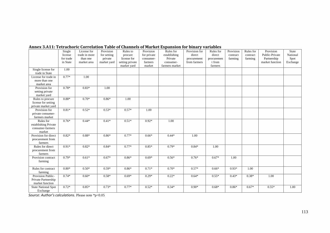
113

Annex 3.A11: Tetrachoric Correlation Table of Channels of Market Expansion for binary variables Single

license

for trade

in State

License for trade in more

than one

market area

Provision for setting

private

market yard

Rules to procure

license for

setting private market yard

Provision for private

consumer-

farmers market

Rules for establishing

Private

consumer-farmers market

Provision for direct

procurement

from farmers

Rules for direct

procuremen

t from farmers

Provision contract

farming

Rules for contract

farming

Provision Public-Private

Partnership

market function

State National

Spot

Exchange

Single license for

trade in State

1.00

License for trade in more than one

market area

0.77*

1.00

Provision for setting private

market yard

0.78*

0.83*

1.00

Rules to procure

license for setting private market yard

0.88*

0.70*

0.86*

1.00

Provision for

private consumer-farmers market

0.81* 0.52*

0.53* 0.57*

1.00

Rules for

establishing Private consumer-farmers

market

0.76* 0.44*

0.41* 0.51*

0.92*

1.00

Provision for direct

procurement from farmers

0.82* 0.88*

0.86*

0.77*

0.66*

0.44*

1.00

Rules for direct

procurement from farmers

0.91* 0.82*

0.84*

0.77*

0.85*

0.79*

0.84*

1.00

Provision contract

farming

0.79*

0.61*

0.67*

0.86*

0.69*

0.56*

0.76*

0.67* 1.00

Rules for contract

farming

0.80* 0.50*

0.59* 0.86*

0.71*

0.70*

0.57*

0.66* 0.93*

1.00

Provision Public-

Private Partnership market function

0.74* 0.60*

0.58* 0.69*

0.29*

0.22*

0.64*

0.55* 0.43* 0.38* 1.00

State National Spot

Exchange

0.72* 0.85*

0.73*

0.77*

0.52*

0.34*

0.90*

0.68* 0.86* 0.67*

0.55*

1.00

Source: Author’s calculations. Please note *p<0.05

114

Annex 3.A12: APMC Rankings, 1970-2008 Year AP As Bi Guj Har Kar MP Mah Ori Pun Raj TN UP WB

1970 7 13 12 6 5 4 10 2 9 1 3 8 14 11

1971 7 14 13 6 3 5 9 2 10 1 4 11 12 8

1972 7 14 12 6 4 5 9 2 11 1 3 10 8 13

1973 6 14 13 7 3 5 9 4 12 1 2 11 8 10

1974 6 14 11 7 3 5 10 4 12 1 2 9 8 13

1975 6 14 8 7 5 3 9 4 12 1 2 10 11 13

1976 6 13 8 7 5 3 9 4 11 1 2 10 12 14

1977 7 11 8 6 3 4 9 5 13 2 1 12 10 14

1978 6 11 8 7 3 4 10 5 14 1 2 12 9 13

1979 6 11 8 7 3 4 10 5 14 1 2 12 9 13

1980 6 11 8 7 3 4 13 5 14 1 2 10 9 12

1981 6 11 8 7 3 5 13 4 14 1 2 12 10 9

1982 7 11 8 9 3 5 13 4 14 1 2 10 12 6

1983 6 11 8 9 3 5 12 4 14 1 2 10 13 7

1984 6 11 8 9 3 5 10 4 14 1 2 12 13 7

1985 7 10 9 6 3 5 12 4 14 1 2 11 13 8

1986 7 11 9 8 2 6 5 4 14 1 3 12 13 10

1987 8 11 9 7 2 6 5 4 13 1 3 12 14 10

1988 7 11 9 8 2 6 5 4 14 1 3 12 13 10

1989 7 11 9 8 2 6 5 4 14 1 3 13 12 10

1990 7 11 10 8 2 6 5 4 14 1 3 12 13 9

1991 8 12 11 9 2 6 5 3 14 1 4 7 13 10

1992 8 12 11 9 2 6 5 4 14 1 3 7 13 10

1993 8 12 11 9 2 7 5 4 14 1 3 6 13 10

1994 8 12 11 9 2 6 5 3 14 1 4 7 13 10

1995 8 12 11 9 2 6 5 3 14 1 4 7 13 10

1996 8 12 11 10 2 6 5 3 14 1 4 7 13 9

1997 8 12 11 10 4 6 3 2 14 1 5 7 13 9

1998 8 12 11 10 4 6 3 2 14 1 5 7 13 9

1999 8 12 11 9 4 7 3 2 14 1 5 6 13 10

2000 8 12 11 9 5 7 1 3 14 2 4 6 13 10

2001 8 12 11 10 5 7 1 2 14 3 4 6 13 9

2002 8 13 11 10 5 7 3 2 14 1 4 6 12 9

2003 8 14 11 10 5 7 3 2 13 1 4 6 12 9

2004 8 14 13 9 5 7 3 2 12 1 4 6 11 10

2005 6 9 13 11 4 8 5 3 14 1 2 7 12 10

2006 6 8 13 11 4 7 5 3 14 1 2 9 12 10

2007 7 9 14 11 5 4 6 1 12 2 3 8 13 10

2008 7 9 14 11 5 2 6 1 12 4 3 8 13 10

Rank change

0 +4 -2 -5 0 +2 +4 +1 -3 -3 0 0 +1 +1

* AP: Andhra Pradesh; Assa: Assam; Bih: Bihar; Guj: Gujarat; Har: Haryana; Kar: Karnataka; MP: Madhya Pradesh; Maha: Maharashtra; Ori: Orissa; Pun: Punjab; Raj: Rajasthan; TN: Tamil Nadu; UP: Uttar Pradesh; WB: West Bengal

Source: Author’s calculations.

115

Annex 3.A13: Seventh APMC sub-dimension: Roads Linking Markets40

0.5

10

.51

0.5

10

.51

1970 1980 1990 2000 2010 1970 1980 1990 2000 2010

1970 1980 1990 2000 2010 1970 1980 1990 2000 2010

Andhra Pradesh Assam Bihar Gujarat

Haryana Karnataka Madhya Pradesh Maharashtra

Orissa Punjab Rajasthan Tamil Nadu

Uttar Pradesh West Bengal

scop

linkin

gm

ark

tnd

ex

YearGraphs by State Name

Source: Author’s calculations.

40 A 7th dimension ‘Market Linking’ was also considered in index construction. It covered length of roads (kms) in the state to proxy for villages connected with the regulated markets but later it was decided to not to add the indicator in the composite index. It was dropped because although State Agricultural Boards and marketing committees in the states are legally responsible to build small patches of roads officially termed as ‘linking roads’ to connect villages to the agricultural market area, the actual variables on ‘linking roads’ is not available. In each state Public Works Department (PWD) department is responsible to construct roads and other public infrastructure. Using the data on length of roads in Kms does not capture the correct intent of the APMC Act. The existing marketing literature informs that existing infrastructure in the states are far from adequate. Nearly half of the villages are still not connected by roads (time-series data is not available). The studies at IFPRI finds that investment in rural roads, both in terms of reduction of poverty and acceleration in economic growth are the highest compared to that in other rural development activities like irrigation, watershed development and education (cited in Acharya, 2006). I show the trends in index of ‘market linking’ measured by (i) Road density (construction/length of roads in the area of per thousand sq kms): It provides the intuition of connectivity of villages to available regulated markets and also points towards progress to achieve the concept of single national market ; (ii) Road length in kms per thousand people/population: It provides intuition for the adequacy of road in the state to serve the population efficiently. It may proxy for level of traffic or congestion on the road that may lead to undue delays in the disposal of the farm produce resulting in long-waiting period and low returns. I do not use it in the APMC index.

116

Chapter 4

4 Do Agricultural Marketing Laws Matter for Rural Growth in India? Evidence from Indian States

4.1 Introduction

In this chapter, I examine the effects of the post-harvest agricultural market

regulations i.e. the APMC Act & Rules, on agricultural development. The evolution of

APMC Act and its effect on agricultural growth is one of the primary issues in India’s

political economy of development. From decades, this specific state marketing

legislation remains central to strategise development of agricultural sector in Indian

states through development of an agricultural marketing system. The role of state in

ensuring market efficiency through institutional framework is regarded in many

historical and contemporary discussions as important as to providing the preconditions

for economic growth (Bardhan 1989; North, 1990; De Long & Shleifer, 1993; Rodrik,

2003; Djankov et al., 2006).

As described in chapter two and three, the issue of legal and administrative framework

of agricultural produce markets is particularly significant in India in the present post-

economic reform period. The agricultural marketing system in India is confronted with

cumulative complex issues associated with marketing of agricultural produce and the

fact that agricultural growth in India has started showing fluctuation and slowdown

since 1990s. Also, the literature on the growing regional divergence in India has failed

to convincingly identify which factor or set of factors may explain the differences in

rate of agricultural performance across Indian states. For instance, during 2000-01 to

2008-09, the growth performance of agriculture in the states of Rajasthan (8.2%), and

Gujarat (7.7%) was much higher than that of Uttar Pradesh (2.3%) and West Bengal

(2.4%) (Eleventh five Year Plan Report, Planning Commission, 2008). The issue of poor

economic performance of agriculture in the states of India is a matter of national

concern at present. The relevance of government interventions, the costs involved and

117

the potential benefits are a subject of heated debate in the policy circle. The opinion is

divided. On the one hand, it is emphasised that the legal and administrative

arrangements i.e. APMC Act, governing agricultural markets need to be strengthened

before growth can resume. On the other hand, a persuasive argument for dismantling

regulatory and administrative structure of the APMC Act altogether in the states is also

observed in a national debate. Though many earlier studies extensively study

agricultural markets of India, there is no contemporary empirical study in terms of

scope and extent to examine if relationship exists between agricultural development

and agricultural marketing regulations as a hypothesis and provide estimates of the

magnitude of such relationship across the Indian states.

In the previous chapter (Chapter three), a composite index is constructed that

quantitatively integrates the six key dimensions of the APMC Act & Rules: (1) Scope of

Regulated Markets; (2) Constitution of Market and Market Structure; (3) Regulating

Sales and Trading in Market; (3) Infrastructure for Market functions; (5) Pro-Poor

Regulations; and (6) Channels of Market Expansion, for select fourteen states between

1970 to 2008 period. Utilising the index, this work investigates the link between APMC

Act & Rules and agricultural productivity in cross-state panel data analysis. The

measure of state-led APMC Act & Rules displays sufficient variation across fourteen

states of India over time 1970-2008 to test whether APMC Act matter for farm

investment decisions and agricultural productivity and also, whether the variations in

APMC measure can explain observed variations in economic performance of

agriculture growth and poverty reduction in the states of India.41

I utilize the composite APMC measure to estimate its effects separately on investment

outcomes such as (i) proportion of gross cropped area which is irrigated; (ii) quantity of

fertilizer used per hectare of gross cropped area; and (iii) the proportion of high

yielding varieties (HYV) of rice and wheat. I also estimate the effects of APMC

regulations upon aggregated agricultural yield productivity, as well as yields for

important staple crops, rice and wheat. Some attempts towards robustness check are

41 In particular the states considered for the analysis are: Andhra Pradesh, Assam, Bihar, Gujarat, Haryana, Karnataka, Madhya Pradesh, Maharashtra, Orissa, Punjab, Rajasthan, Tamil Nadu, Uttar Pradesh and West Bengal. Together they represent around 94% of Indian population

118

made by using different model setting such as exploring the causal relationship using

APMC sub-indices and instrumental variable estimation. The impact of APMC measure

on poverty reduction is also investigated. A production function analysis which is

conventionally explored in the literature is modelled in determining the relationship of

APMC regulations with both agricultural investment and productivity yields variables

at the state level. Following Adams and Bumb (1979), it is assumed that economic

policy at a state level will affect individual farm decision in systematic ways. For

instance, a number of policy action – such as subsidy on irrigation and power or public

investment on farm infrastructure, cooperative credit provision and the like – reflect

policy choices of state authorities that influence inter-state yield comparison and

related farm decisions (Ibid).

The chapter is organised in nine sections. In the next section, I describe the conceptual

basis of why APMC measure i.e. regulations of agricultural markets may matter for

agricultural performance. In section 4.3, following Mundlak et al., (2012), theoretical

and statistical model predicting that agricultural outcomes are driven by variations in

the APMC regulations across the states is presented. Section 4.4 describes the

econometric methodology and discusses the empirical specification. In section 4.5, I

describe the data and variables used in the empirical analysis. Section 4.6 presents the

results of the empirical analysis. Section 4.7 presents results from robustness checks

such as using APMC sub-indices, and instrumental variable estimation. In section 4.8,

poverty implication of the APMC measure is explored. Section 4.9 concludes.

4.2 Why should legal Framework Regulating the Agricultural Markets Matter for Economic Performance of Agriculture sector? Conceptual Literature

The legal framework of regulations of the agricultural markets affects agricultural

productivity in a number of different ways (Schultz, 1978a,b; Acharya, 2004).

Regulations can be primary means of regulating the behaviour of participants in

agricultural markets and the consequences of their actions (Cullinan, 1999). They can

help in building capacity of individuals through collective action and can have

accelerating effect on agricultural productivity and economic growth (Acharya, 2003).

119

The literature describes that, first, good quality agricultural laws regulating the

agricultural markets channelize farmers to allocate the resources according to their

comparative advantage and to invest in modern farm inputs to obtain enhanced

agricultural productivity. This leads to increased market surplus of farm produce and

increased regional trade in turn creating demand for more markets, meaning

transformation of agriculture from subsistence vintage to an increased commercial

enterprise; and second, the adoption of improved agricultural technologies depends

also on marketing infrastructure. Thus, strengthening of legal and administrative

framework with a well spread-out and regulated infrastructure of agricultural produce

markets acts as an incentive to induce use of inputs and improved technologies all

resulting in increased agricultural productivity and economic growth (Rao et al., 1984).

Every market system generates impulses within the context of a given regulatory

institutional framework that may lead to increased output by releasing the forces of

production (Bhalla, 1988). To put in other way, if the additional produce in the

regulated agricultural markets does not move to bring additional revenue to the

farmers, it may send out wrong signal of production saturation and might work as a

disincentive to increase further production. If the system does not supply foodgrains

and other agricultural commodities at reasonable prices to the people at the time and

place needed by them, increased production has no meaning in the welfare society. It

may even cause a sort of disruption in social equilibrium of the society. Lastly, of all if

agricultural growth is affected, it has direct impact on sector’s progress to which the

overall growth of the Indian economy is linked (Chand, 2005a; Acharya & Agarwal,

2009).

The efficiency of the agricultural marketing may be understood as the effectiveness or

competence with which the market administration under the regulatory framework of

the APMC Act performs operations to accomplish the defined objective of providing

efficient services in the transfer of farm products and inputs from producers to

consumers, while safeguarding the interest of all three indispensible groups associated

in marketing, i.e. cultivator- farmer, consumer and trader. The whole marketing

mechanism functions in a way to provide the maximum share to the cultivator-farmer

in the consumer’s rupee; food and other farm products of required quality to

120

consumers at the lowest possible price; and enough margin to traders in the middle

that they remain in the trade (Acharya & Agarwal, 2009). The expectations of the three

groups from the system are in conflict. The efficiency and success of the system

depends on how best these conflicting objectives are reconciled. In view of an

important step to increasing efficiency of market channels is to promote regulations of

market places (Rao et al., 1984). Agricultural regulations can provide a structure

safeguarding the interest of all groups associated in marketing and to increase the

efficiency of farm investment and of overall agricultural productivity growth in the

economy.

The literature in economics of agricultural development shows numerous different

ways unveiling the role of agricultural institutions in economic behaviour. This includes

recognition of the importance of farm policies and food regulations in affecting crop

acres, asset management, intensive and extensive margin decisions, risk management

choices in agricultural production, land property rights and other transaction costs and

contractual arrangements (such as Binswanger & Rosenzweig, 1986; Stiglitz, 1988;

Bardhan, 1989; Nabli & Nugent, 1989; Harriss et al., 1995; Fafchamps, 2004; Rozelle &

Swinnen, 2004; LaFrance et al. 2011).

According to the literature, the challenge of ‘low level equilibrium trap’ of a low

income economy can be investigated by the study of regulatory arrangements of

agricultural marketing system. The mechanism by which inefficient law or institution

negatively impacts economic growth can be illustrated that a poor income state

suffering from ‘weak’ institutional environment tends to generate low economic

activity. Low levels of economic activity can on its own give way to thin markets,

inadequate coordination, high transaction costs and risks and high unit costs for

infrastructural development. The result can then easily be a low equilibrium trap

(Dorward et al., 2003). Similarly, the market players particularly those with little

financial and social resources or political leverage face high, often prohibitive, costs in

accessing information and in enforcing property right when the institutional

environment and arrangements are weak. The costs then inhibit both technological

adoption and economic development (Ibid; Dorward & Morrison, 2000; Dorward et al.,

2004; Dorward et al., 2005).

121

An absence or an inappropriate legal framework can undermine the prospects of

achieving desired policy objectives, introduce unnecessary distortion and reduce the

efficiency of the market, increase the cost to the participants and severely stunt the

development of a healthy agricultural sector (Cullinan, 1999). Regulations that

establishes the agricultural markets create channels to connect producers and

consumers overtime (storage) and space (transport), and along this channel the

agricultural product is transformed into a consumable product (processing) (Chand,

2005b). It helps in optimization of resource use, output management, increase in farm

incomes, widening of markets, growth of agro-based industry, addition to national

income through value addition and employment creation (Acharya, 2006). Thus,

regulatory framework of agricultural markets in Indian states can be expected to

increase the efficiency of farm investment and of overall productivity growth in the

agriculture sector.

4.3 Theory and Choice of Statistical Model Framework

Although literature on agricultural growth shows increasing role of research and

technological factors as driving source of both agricultural production and productivity,

much of the increase in knowledge and application of new techniques are adopted

unevenly in the countries. Agricultural techniques differ across and within countries.

For empirical analysis, it has been conceptually difficult to account for changes in

agricultural productivity as a function of usage of various agricultural inputs (Haley,

1991).

Much of the research studying the agricultural production function in low income

countries began with Schultz (1964). The main argument in his work stresses that

agricultural technology that drives agricultural growth always embodied in factors or

agricultural inputs. Technological change therefore should not be treated as residual

from econometric estimation of production function. In his future works, Schultz

(1978b) argued that difference in the productivity of the soils or other geographical

aspect is not a useful variable to explain why people are poor in long-settled parts of

the world. “What matters most in the case of farmland are the incentives and

associated opportunities that farm people have to augment the effective supply of

land by means of investments that include the contributions of agricultural research

122

and the improvements of human skills” (Schultz, 1979). These incentives are explicit in

the prices that farmers receive for their products they produce and in the prices they

pay for consumer goods and services that they purchase (Schultz, 1978a,b).

Hayami & Ruttan (1971) building upon Schultz’s work introduced a ‘metaproduction’

(aggregate homogeneous) function to measure the determinants of agricultural

development for all countries (developed and developing) in a sample. The approach

was based on the assumption that all countries have access to same technology but

each may operate on a different level of the function due to specific country situations.

Hayami & Ruttan (1971) described the metaproduction as an envelope of all

commonly conceived neoclassical production function. The research emphasized that

agriculture adapts to changes in profitability by adjusting to a more efficient point on

the metaproduction function. The readjustment acts through changes in the return to

factors which are specific to agriculture. If the changes in profitability are perceived to

be long lasting, then factor reallocation will take place. The reallocation of factors will

affect the nation’s ability to produce agricultural commodities. The metaproduction

function is thus like an efficiency frontier. The position on which a country finds itself

depends on factor price ratio in that country (Haley, 1991). They argue that

technological changes are therefore endogenous to the economic system.

Mundlak & his co-authors (1982; 1988; 1997; 2012) criticise the approach used by

Hayami & Ruttan. They argue that it is more than differing factor price ratios that can

explain differing input-output relationships. Mundlak’s starting point is that farmer-

producers face more than one technique of agricultural production. Because the

economic environments within which farmer-producers operate differ, they make

different choices from a given set of techniques. So the implemented technology of

agricultural production is heterogeneous (and not homogeneous). Technology is

therefore a collection of techniques which are available for implementation. The

motivation for changes in implemented techniques depends more importantly on the

economic environment which is predetermined by state variable such as economic

policy. Here in this research, it is regulatory institution i.e. APMC Act & Rules of the

agricultural markets.

123

According to the model, the adaption of a new technique does not exclude the

possibility that existing capital is already committed and therefore there can be

simultaneous use of differing techniques (use of traditional and modern technique) in

a country. Based on Mundlak’s analysis, this research conceptualised that the changes

in the level of APMC measure in a state can cause a reallocation of already committed

capital into forms which constitute techniques different from those previously used.

The strength of regulatory framework of the APMC measure determines state’s

(farmer-producer) capacity to absorb advances in agricultural technology. As the

objective of this chapter is to estimate role of APMC legal institutions in determining

agricultural output differences in the panel data form, Mundlak et al, 2012 (originally

Mundlak, 1988, 1997) approach fits well.

4.3.1 The Model Framework

Following the pioneering work of Mundlak (1988), variability of agricultural production

function across states in India is assumed to be based on a view that technology is

heterogeneous and the choice of technology is determined by the economic and

physical environment. In this chapter, I use a modified version of Mundlak et al (2012)

to formulate the problem in a way that allows to empirically estimate agricultural

productivity by integrating index of regulations of the agricultural markets (APMC

measure) into the function. The meaning of the production function is clear when it

describes a well defined process (Haley, 1991). In agriculture, this process could be the

production of a crop under a set of well defined conditions. But in agriculture, there

are many types of crops as well as livestock and many different sets of environmental

conditions. This observation implies that there are a myriad of agricultural production

functions. The estimation of a production function is then based on the assumption

that a well defined production function holds up to a random error which is associated

with a given input requirement set. The building block of this assumption is that

farmer-producers any time face more than one technique of production and their

economic problem is to choose the techniques to be employed along with the choice

of inputs )(X and output )(Y . A technique represents the most basic process of

production and it is denoted by a production function )(XFj associated with the

thj

124

technique, where jF is concave and twice differentiable42 function of input X . The

available technology )(Tn is collection of all possible techniques,

}....1);({ JjXFTn j and thus represents the threshold of knowledge in a state.

Firms choose the implemented techniques subject to their constraints and the

environment within which they operate.

I present motivation for the model’s solution and its implications, directing to Mundlak

(1988) for modelling derivative details. Let W and P be the prices of inputs and output

respectively. K represents policy or regional constraints on inputs such as APMC Act &

Rules. Let ),,,( TnWPKs represent the vector of state variables for this problem.43

The solution 0)(* sX jis the optimal level of inputs allocated to technique j. Given a

function, the optimal output of technique j is )*(*j

Xj

Fj

Y and the implemented

technology )(ITn is the collection of the implemented techniques, in symbol,

},0)*();({)( Tj

Fj

Xj

Fj

Xj

FsITn .

Simplifying the analysis, an available data shows inputs and output only at the firm

level and not by techniques. Therefore, a firm level represents the most basic

component. The aggregate production function expresses the aggregate of outputs,

produced by a set of microproduction functions, as a function of aggregate inputs. This

function is not uniquely defined because the set of micro functions actually

implemented and over which the aggregation is performed, depends on the state

variables and as such is endogeneous. Let’s assume that the optimal output over

techniques can be summarized by the following function:

)(),( ** ssXFY (1)

42 Twice differentiable function is a function that is differentiable and that has a differentiable derivative. A function whose second derivative is non-positive everywhere (for all x) is concave. The importance of concave in optimization theory comes from the fact that if the differentiable function (f) is concave then every point x (level of inputs) at which f '(x) = 0 is a global maximizer of output/profit. 43 Mundlak et al., (2012) refer to the State variables that characterise the initial economic conditions that influence producer choices but are exogenous from the perspective of the firm or households (2012:1).

125

Where, *X is the vector of the optimal inputs aggregated over the implemented

techniques. The function is defined conditional on s . Changes in s imply changes in

*X , as well as in ),( * sXF , and this is summarized by the reduced form )(s . The

dependence of the inputs and the implemented technology on is referred to as the

jointness property. The implication is that whenever the implemented technology is

affected by state variables, it is not possible to reveal empirically a stable production

function from a sample of observations taken over points with changing available

technology. Consequently, in general the aggregate production function is not

identifiable.44 Complicating empirical model, the planned solution values of the

optimisation problem are not observed because outcomes are stochastic. Thus, the

production function can be examined only with inexact observed data. The empirical

aggregate production function can be thought of as an approximation in a specific way.

00)()(ums eXsY

(2)

Where Y and X are observed over techniques, 0m is an idiosyncratic term known to

the firm, thus affecting the firm’s decision but unknown to the econometrician. The

random term 0u is unknown to both the econometrician and the firm at the time the

production decision is made and is uncorrelated with the inputs. nueEe 0 is constant,

and without a loss in generality, it is absorbed in )(s

It has been shown (Mundlak, 1988) that the efficiency frontier of the implemented

technology i.e. ),( * sXF can be approximated by a function which looks like a Cobb-

Douglas function, but where the elasticities are functions of the state variables and

possibly of the inputs:

XXssY ln),()(ln (3)

44 An important implication of defining the production function in this way is that total factor productivity and the marginal product of the choice variables depend on the state variables. This production function is defined conditional on s.

126

Where Y is the value added per hectare, ),( Xs and )(s are the slope and intercept of

the function respectively and is a stochastic term. In other words, from equation (2) and (3)

the expectation of output, conditional on sX , and 0m is )(sY e 0)( ms eX and the

choice criterion is )(max)|( WXPYsX e

x

e . It means output (P) is the price of X

measured in units of Y. The generic form of the first order condition yields the optimal

input *X conditional on s , 0m and P .45 This model implies that variation in the state

variables affect intercept )(s and slope ),( Xs of the function directly as well as

indirectly through their effect on inputs. The innovation in this formulation lies in the

response of the implemented technology to the state variables. When the available

technology consists of more than one technique, a change in the state variables may

cause a change in the composition of techniques in addition to a change in input used

in a given technique. In this case, the empirical function is a mixture of functions and

as such may violate the concavity property of production function.46

In next sub-section, the model is employed to investigate the role of the state

variable: APMC Act on agriculture performance using data.

4.4 Empirical Analysis

4.4.1 Empirical Model Specification and Estimation methods

Following Mundlak’s (2012) simplified solution of the system for panel data analysis,

reduced form of output equation (1) is estimated, which amounts to quasi-supply

function, in the sense that it allows for changes in the supply function. The

dependence of the implemented technology on the state variables (for example,

APMC measure) causes it to vary across states and over time in any given state. In

writing the system solution, it is assumed that the level effect of the APMC measure on

farm inputs and output is linear (Ibid). The model, indicating the dependence of

agricultural outcomes (such as yield productivity, input-investment decisions) on the

state variable: APMC Act & Rules of the agricultural markets, can be reformulated in

the reduced form panel data equation, such as equation A and B, as specified below.

45 Model focuses on p, but analytic detail applies to the ratio p/w (price of output/price of inputs) (Mundlak et al., 2012). 46

The procedure is described in detail in Mundlak (1988).

127

The empirical approach here is to run panel data regression to examine the temporal

effect of APMC measure independent of other factors that have been found to

determine agricultural growth across Indian states and over time. Two forms of panel

data approach is taken in the analysis: Standard Fixed Effects Model (FE), as shown in

equation (A) and Feasible Generalised Least Squares (FGLS) approach, as shown in

equation (B). Both are acceptable methods to deal with often encountered panel

issues such as panel heteroscedasticity, the subject that will be discussed later in the

methods section.

The generic inter-state panel equation for the two approaches can be formulated as

equation A (FE) and as equation B (FGLS):

ittiititit εμνAPMCβXββY 5210 (A)

ititititit statedummyyeardummyAPMCY 435210 (B)

Where in both equation (A) and (B) for state i at time t (denoting year), itY is some

log-linear or ratio measure of agricultural outcome. s' are the parameters to be

estimated. itX is a vector of variables in log-linear or ratio form that I treat as

exogeneous (detailed later).47 In equation (A) tμ and iν capture the time-invariant and

state-invariant components of the error term respectively, while it accounts for white

noise of the error component. In equation (B), taking the form of FGLS panel data

regression model, state dummy denotes a state fixed effects and a year dummy

variable denotes time fixed effects. it is the error term that allows for a

hetroskedasticity in error structure with each state having its own error variance.

Equations (A) and (B) are generic inter-state panel data econometric specification

47 Indian states vary in size and performance. Data set on some of the variables are needed to be proportionate to size of the state and therefore ratio (share in total) is used to obtain comparative data sets across the states. Given some variables are measured in ratio data and appear in decimals, it is desirable to avoid negative logarithms. Consequently, though consistent with earlier authors (Lin, 1992; Frisvold & Ingram, 1995; Appleton & Balihuta, 1996; Mundlak, et al. 2012) some non-conventional input variables are measured in proportions (as described in data section).

128

which forms the base to examine the effect of APMC measure on different input

investment decisions and yield productivity outcome variables in the chapter.

In all the regression equations, the key coefficient of interest is52 itAPMC (as

captured in chapter 3 which measures regulatory practices and rules that guide code

of business of agricultural produce markets in state i at time t ). Following Besley &

Burgess (2000 & 2004) who use time lags in their institutional variable (e.g. land

reform legislation and labour laws in context of Indian states) to study relationship

between legal institution and economic output, measure of the APMC Act is lagged by

five-year time periods. Five year period time lag in the APMC index is chosen for two

main reasons. First and foremost reason is that any legislation (even the effective one)

will take time to be implemented and to have an impact. Second, time lags help to

address econometric concerns that any form of shock (other policy treatment or

natural weather shock) to agricultural growth outcome will be correlated with APMC

reforms efforts. It implies that by taking lags, universal concern that APMC measure

could be endogenous to economic conditions and it is probably responding to the

same forces that drive agricultural outcomes is tackled, an issue to which I return in

sub-section 4.7.2. Different choices like discussions with experts during the field work,

review of literature and data structure guided in both to use lags as well as to

determine the 5-year time lag structure of the APMC measure in the analysis.48,49

48 Different form of lag structure is tried to make a careful selection. The results are robust to imposing different lag structure in all the outcome variables except in the case of aggregate foodgrain yields. With lag lesser than 5 year-period, I get significantly negative relationship between the APMC measure and the yield productivity, indicating reforms in market acts may take time to impact economic activities positively and initial phase of economic reforms may even cause some costs before economic growth respond to it optimally. Also, the risk response literature suggests that farmers can take time to make decision with respect to their farm management. The number of years ahead over which the farmer as a decision maker evaluates the consequences of alternative actions (invest now or postpone the decision) may influence the choice of the preferred decision alternative (Backus et al., 1997:312). This suggests that farmer looks for market environment to be conducive and predictable. The intermediate time period (time-span before the law is firmly enforced in the market) when a reform in the law is introduced might also create a situation of uncertainty in the market. Knight (1921) divided decision-making situations into risk and uncertainty. The risk situation is the one in which decision-maker knows both the alternative outcomes and the probability associated with each outcome. Under uncertainty, the decision maker does not know the probability of alternative outcomes. In this view, it is possible that immediate institution of the reformed APMC Act (associated with lesser time lag) might not lead towards positive outcomes. In anticipation of uncertainty or fear of an adverse effect of the reform may give rise to a speculative action disrupting the normal function of the law, and thus failing to do what the law is suppose to do.

129

4.4.1.1 Relationship between Farm Input Investment Decisions and APMC Act in Panel Data Model

Using the model specification (A) & (B), firstly, four empirical equations of farm

investment decisions are estimated. For all four equations, I applied least squares

dummy variable (LSDV) estimator, which is an alternative way to estimate parameters

of the fixed-effects models. LSDV estimator is applied mainly to retain the effects of

geographic variable which is fixed over time in the states. The coefficient estimates

and standard errors are exactly the same as those obtained from Fixed Effects (FE)

estimator. I also run the same regression using FGLS approach. I discuss the technique

of FE and FGLS model in sub-section on methods

Dependent Variable itY

Each time in equation A & B, itY is an outcome variable representing individual state

decision to make a farm investment, where itY represents:

itusesFertilizerLn )_( captured by natural logarithm of use of fertilizer in kilograms

per hectare of land in state i at time t ……………………..(Equation 1)

itAreaIrrigatedofproportion ___ captured by percentage of land irrigated of the

total gross cropped area in state i at time t…………………………….(Equation 2)

itHVYriceunderArea __% captured by percentage of land area under high yield

variety of Rice in state i at time t……………………………………… (Equation 3)

itHVYwheatunderArea __% captured by percentage of land area under high yield

variety of Wheat in state i at time t…………………………….. (Equation 4)

49 APMC index is lagged by five year time period in all the regressions that I run using various outcome variables (investment, yield and poverty). I get significant results and right sign for the input variables when shorter time lags are used. It is possible that some crops or inputs might respond quicker than others to regulatory conditions of the agricultural market. Nonetheless, same lag structure is kept throughout the analysis in order to maintain consistency and ensure robustness of the results.

130

Other Explanatory variables in itX vector

In the four empirical equations of farm investment 1-4, itX is a vector of explanatory

variables that may affect investment decision. Following the empirical literature on

farm investment decision and institution, specifically in line with Banerjee & Iyer

(2005), in the specification farm investments (such as use of fertilizer, irrigated land,

high yield variety crops), are posited to depend on institutional framework of the

APMC measure and variables of state level physical environment. Since use of farm

inputs depends on natural conditions of the state, I include a dummy on coastal

environment capturing whether the state has coastal environment or not, average

farm land measuring average farm size in hectare of land, and average rainfall, which is

a natural logarithm of annual average rainfall in millimetres.50 Mundlak et al., (2012)

controls for geographic variables in the set of ‘state variables’ in the model along with

the variable of agricultural economic policy. Here, measure of APMC index is the key

state variable as discussed in the model framework.

I also include a variable on state’s literacy rate in the model specification to control for

the role of education in adoption of modern farm practices and agricultural

innovations (Schultz, 1988; Feder et al., 1985; Appleton & Balihuta, 1996).51 The

dependent variables in the analysis of farm investment decisions represent the

modern commercial agricultural inputs (chemical fertilizer, machine irrigation, and use

of research based HYV crops). Literature discusses both cognitive and non-cognitive

effects of literacy on use of farm inputs to raise agricultural productivity. Literacy

enables one to follow written instructions for chemical inputs and other aspects of

modern farm technology that may increase productivity produced by a given

combination of inputs (Harma, 1979; Appleton & Balihuta, 1996). Feder et al, 1985

finds that educated farmers tends to adopt agricultural innovations, for example

modern inputs or new crops. Education may also have non-cognitive effects, changing

people’s attitudes and practices. Appleton & Balihuta (1996: 417) maintain that in a

50 Unlike Banerjee & Iyer (2005), I could not include some geographical variables such as type of top soil, latitude, altitude due to lack of ready availability of the state-wise data on them. 51 The working definition of literacy rate in the Indian census since 1991 is the total percentage of the population of an area at a particular time aged seven years or above who can read and write with understanding.

131

developing country, education increases people’s achievement orientation, with

greater awareness of the opportunity to improve one’s living standard. There may be

greater openness to new ideas and modern practices. Against this, it is also argued

that education leads to a disdain for agriculture, as students aspire to formal sector

employment. Also, the extent to which farmers are able to use new technologies to

their advantage depends on the learning about costs and benefits of using new

technologies (Antle, 1983). It is, therefore, possible to find a negative coefficient on

education variable in the regression.

4.4.1.2 Relationship between Farm Yield Productivity and APMC Act in Panel Data Model

Next, I investigate empirically implications of APMC Act on aggregate agricultural yield

productivity and yields for important staple crops, rice and wheat, using the model

specification (A) and (B) of panel regression.

Dependent Variable itY (Yield Productivity)

Each time in equation A & B, itY is the main agricultural outcome variable that

represents:

itYieldsLn )( measured as the natural logarithm of aggregate yield of principal

foodgrains per hectare in kilograms in state i at time t………………(Equation 5)

itYieldWheatLn )_( measured as the natural logarithm of wheat per hectare in

kilograms in state i at time t……………………………………………..(Equation 6)

itYieldRiceLn )_( measured as the natural logarithm of rice per hectare in kilograms in

state i at time t…………………………………………….(Equation 7)

132

Other Explanatory variables in itX vector

In the three empirical equations 5-7, itX is a vector of explanatory variables based on

the existing literature on agricultural growth regression. The earlier studies explain

sources of agrarian growth productivity in different parts of India by use of variables

that relates to investments ‘in’ farm inputs (such as irrigation; fertilizer) and

investments ‘for’ agriculture (such as research and development of technology,

infrastructure etc) (Dantwala, 1986; Chand, 2005a; Fan, Gulati & Thorat, 2007).

Literature shows that agricultural productivity can be brought through increase in

intensity of cultivation by use of modern inputs (Mundlak et al., 2012; Chand et al.,

2007; Adams & Bumb, 1979. In line with it, the baseline specification includes, use of

fertilizer, measured as the natural logarithm of use of fertilizer in kilograms per hectare

of land, area under irrigation, measured as a percentage of land irrigated of the total

gross cropped area and capital, measured as an index of number of pump-sets and

number of tractors per thousand hectares of land, computed by principle component

analysis (PCA technique); State-specific natural logarithm of average annual rainfall in

millimetres per year is also included to take into account the differential effects that

variations in rainfall across India for a particular year may have on state-level

agricultural productivity (Cali & Sen, 2011). I also include a variable on labour,

measured as natural logarithm of number of agricultural labourers per thousand

hectares of gross cropped area in the baseline specification. It controls for

economically active population in state agriculture in the year and proxies state’s

resource endowment (Bhalla & Singh, 1997; Chand et al.,2009).52

Some studies observe the use of technological innovations such as new crop varieties

specifically for rain-fed, dry-land and other ecological settings helps in picking up the

growth in low productivity area. It can narrow down regional differences in agricultural

productivity across states that occurred after initial phase of green revolution of 1960s

(Sawant & Achutan 1995; Bhalla and Singh, 1997). Chand (2005a) reports that even in

agriculturally advanced state like Punjab the actual yield of paddy can be raised by 87%

52 High correlation between farm inputs and literacy variable creates a potential problem of multi-collinearity in the regression using both farm inputs and literacy. Therefore, I control for key farm inputs and not education to affect agricultural productivity.

133

using the existing improved technology. In most of the crops, technologies are

available to double the actual yield in the various regions of India. Yield productivity

can be increased by investing in agricultural technology such as short duration

cropping seeds (Chand et al., 2007). To capture use of such technology innovation, I

account for cropping intensity which is measured as natural logarithm of gross cropped

area (GCA) subtracted by net cropped area (NCA) (based on Chand et al., 2007).

Intuitively, the measure of cropping intensity captures number of times land is sown by

using new variety seeds in a year.

In an expanded specification, based on earlier works I add three more variables:

landholdings (average farm-size), road density (length of the roads in kilometres per

thousand population) and annual per capita state expenditure on agriculture sector.

I control for size of the farm land to capture efficiency effects on productivity. In India,

the average size of operational holdings has diminished progressively from 2.28 ha in

1970-71 to 1.55 ha in 1990-91 to 1.23 ha in 2005-06. As per Agriculture Census 2005-

06, the proportion of marginal holdings (area less than 1 ha) has increased from 61.6

percent in 1995-96 to 64.8 percent in 2005-06. Fragmentation of operational holdings

has widened the base of the agrarian disparity in most states. Empirical studies have,

however, demonstrated that agricultural productivity is size neutral. Many modern

studies provide evidence specifically from a range of developing countries, including

India, demonstrating that small farms are more efficient in increasing farm productivity

(Berry & Cline, 1979; Saini, 1979).

Empirical works show the infrastructure effect (public-sector investments) is

associated with augmentation in agricultural productivity potential (Gulati & Bathla,

2001; Fan, Gulati & Thorat, 2007). Two variables are included to capture level of

infrastructure in a state: one, I include a variable on state budgetary expenditure on

agricultural and allied services in per capita terms that may proxy for government’s

efforts to develop infrastructure exclusive for state agricultural development; and two,

I take into account the role of road density measured as length of the roads in

134

kilometres per thousand population in influencing agricultural productivity.53 This

variable controls for returns from adequacy of road in the state to serve the

population efficiently. It may proxy for level of traffic or congestion on the road that

may lead to undue delays in the disposal of the farm produce resulting in long-waiting

period and low returns on quality grounds. It will ultimately influence the incentives to

increase farm productivity. Also, much of the cultivated area is remotely located from

the markets, which makes efforts to increase productivity strongly dependent on

infrastructure. Being far from the market helps to create local monopolies, decreases

the competitive process in the industries serving agriculture and increases the cost of

services. The weak market connection encourages production for self sufficiency. Such

production is expected to be less susceptible to market conditions (Mundlak, 2000:19).

Studies find that investment in rural roads, both in terms of reduction of poverty and

acceleration in economic growth are the highest compared to that in other rural

development activities like irrigation, watershed development and education

(Binswanger et al., 1993; Fan et al., 2000; Acharya, 2006).

Finally, in all regression equations (1-7), the year fixed effects are included to capture

any annual idiosyncratic national-level common shocks such as oil-price shocks and

other macroeconomic policy shocks that affect productivity output across all states in

a given year (Besley & Burgess, 2004; Cali & Sen, 2011).54 For instance, although

agricultural marketing is a state subject, the union government plays an important role

in designing its policy framework. In addition to the Planning Commission which

determines the sectoral and regional allocation of resources and the Ministry of

Finance which is responsible for fiscal and monetary policies that have direct bearing

on the agricultural sector, the three other union ministries have a predominant role in

the functioning of the agricultural marketing sector: The Ministry of Food; The Ministry

of Agriculture and the Ministry of Civil Supplies, Consumer Affairs and Public

53 I do not deflate road density variable with land area because such indicator would inadvertently measure the distance from the non-crop area or inhabitant area, which is less desirable when infrastructure is inadequately developed in the state to serve the population. 54 Statistical test for joint significance of time fixed effects with the full model specification (with all controls) is undertaken. STATA offers an option to test if time fixed effects are needed when running a FE model. The null hypothesis in the test is that dummies for all years are jointly equal to 0. If the test fails to reject the null, then time fixed effects are not needed. I get strongly significant results with overall statistics: F (33, 419) = 2.78 and p = 0.0000, which imply inclusion of the year time effects in the model

135

Distribution (Kohli & Smith, 1998). Therefore, it is likely that measures of relationship

between the APMC measure and agricultural productivity appear spurious if year

effects are not taken into the account.

The state fixed effects controls for unobserved, time invariant differences such as

specific cultural and geographic characteristics that may have impact on agricultural

performance across Indian states. The Indian states are known for their diversity in

terms of resource endowments, climate, geography and topography other than

institutional and socio economic factors (Chand et al., 2009).

4.4.2 Econometric Estimation Methods

To estimate equation (A) specified above, I use fixed effects panel data analysis. As

mentioned, the econometric interest lies in comparing long-run agricultural

investments and yield productivity levels across the Indian states on the basis of

difference in the respective state’s APMC Act. The panel data technique is the standard

econometric approach in research tasks like the one being dealt here. Here the

methodological concern is that estimates on the APMC measure or other explanatory

regressors used in the model for the agricultural outcome might be driven by some

omitted or unobserved state characteristics (such as history, culture or, differences in

farm traditions and practices across states, social norms, farm managerial skills, etc).

And as is well known, in such a case where individual unobserved state differences

might be correlated with both the APMC regulations and the agricultural outcome

variable, estimates would not reflect the true impact of APMC Act on agricultural

outcome.

The panel data fixed effect method subsides or limits the problem of omitted or

unobserved farm specific variables (assumed to be time- invariant over time) in

estimating common relationships across states. It is useful in the sense that the

technique, by virtue of its estimation process, takes into account the presence of

endogeneity of correlation between the unobserved state-specific heterogeineity and

the explanatory regressors. Thus, this econometric feature of FE panel data method

allows to predict economic phenomena, such as economic implications of the APMC

136

measure, more accurately. Observing fixed effects approach also likely to clean state-

specific idiosyncrasies in the dataset used to compute the APMC index by removing

time-invariant state-specific features (Judson & Owen, 1999; Hasio, 2003). Moreover,

the Hausman test also statistically confirms the use of fixed effects model technique

over an alternative panel data model: random effects model for the analysis. 55

As noted, an alternative form of panel data approach: Feasible Generalised Least

Squares (FGLS) approach is additionally used in the analysis. Equation (B) is estimated

using FGLS approach which also provides for testing of robustness of the results.

In present case, there is a need to take caution in the panel structure of the dataset,

especially a long panel dataset that this work uses for the analysis. In a long panel, like

the one used in the work, with many time periods for relatively few states (N is small

and T → ∞) non-identically distributed (iid) errors (hetroscedasticity) and identically

dependently distributed errors (autocorrelations) are often an issue in the analysis of

panel data. There could also be a correlation or dependency among the errors of the

same cross-sectional unit, though the errors from different cross-sectional units are

independent. For instance, in this specific case, a possibility of the presence of complex

patterns of mutual dependence between the cross-sectional units of the panel

datasets through social learning, herd behaviour and neighbourhood effects especially

thinking in context of rural settings in the Indian states can exists. Therefore,

erroneously ignoring possible correlation of regression disturbance over time and

between states (subjects) can lead to biased statistical inference (Driscoll & Kraay

1998; Baltagi, 2005; Hoechle, 2007).

As suspected, the requisite diagnostics (see Annex 4.A1) show that the panel

hetroscedasticity and cross-sectional dependency are statistically significant in the

data structure. Under the fixed effects classical OLS model that I undertake in this

55 Random effects panel data model are used when it is taken to assume that there is no correlation between the unobserved state-specific characteristics and the explanatory variables. In the present case, the overall test statistics for model selection: chi2(43) = (b-B)'[(V_b-V_B)^(-1)](b-B) = 34.78, Prob>chi2 = 0.8097 (comparing the coefficient estimates of the two model) rejects the null hypothesis of unique errors (unobserved individual effect) to be uncorrelated with the regressors (independent variables) included in the model (Hausman, 1978). Hence, statistically also, FE model estimation is preferred method for the analysis.

137

work, I still get unbiased and consistent estimator but it is inefficient under the class of

linear unbiased estimators. As regards detaching panel hetroscedasticity, there are

several acceptable estimation methods to deal with the problem of panel

hetroscedasticity. Following some of the existing panel data research analysis: Besley

& Burgess (2000); Lio & Liu (2006); Mundlak et al., (2012), a more-efficient Feasible

Generalised Least Squares (FGLS) estimation as a supplementary technique is used

which allows for richer models of error process than those specified in the short-panel

case to ensure validity of the statistical results (Wooldridge, 2002). It estimates a panel

model in the presence of panel heteroscedasticity.

The FGLS is recommended technique for a long panel that satisfies the classical

assumptions with modifications to allow stochastic regressors and non-normality of

errors (Amemiya, 1985; Greene, 2003; Frees, 2004). Estimation via FGLS method

allows the error it in the model to be correlated over i (individual state) and allows

for a hetroskedasticity in error structure with each state having its own error variance.

It also allows to model error term it as AR(1) process where the degree of auto-

correlation is state-specific, i.e. ititiit 1 . As noted, both state and time fixed

effects are controlled in the model by including dummy variables for each state as

regressors (Maddala, 2001, Torres-Reyna, 2012.56 In the literature, although FGLS

method is used in random effects models (RE) to account for particular type of

correlations among the errors in these models, Maddala (2001) explains that FGLS

method is consistent in fixed effects (within group estimation) whether the key

assumption under the RE model – ( i are not correlated with itx ) – is valid or not,

since all time-invariant effects are subtracted out and as T gets larger, FGLS and FE get

closer (Maddala, 2001:578).57 On general terms, after algebraic simplification, the FGLS

regression can be interpreted as a weighted linear regression of iy on ix with the

weight )(1 ii zw assigned to the thi observation.58 In practice, )( iz may depend

on unknown parameters leading to the feasible GLS estimator (Baltagi, 2005). Fuller

56 http://dss.princeton.edu/training/ (source) 57 Maddala (2001:578) gives the statistical derivative proof showing that estimates from the random effects model and fixed effects model are the same. 58 According to Maddala (2001), the OLS and LSDV estimators are special cases of the FGLS estimator.

138

and Battese (1973), show that the FGLS estimator is the same as the OLS estimator

from the transformed data.

In the empirical analysis, where data structure allowed, both FE and FGLS panel data

regression are run for the analysis. Regression results from use of both FE and FGLS

methods are reported in the results’ tables. In the work, according to the Gauss-

Markov theorem, FGLS transformation estimation is more efficient than FE OLS

estimation in the linear regression model, leading to smaller standard errors, narrower

confidence intervals and larger t-statistics (Wooldridge, 2002). I, therefore, discuss the

estimated results based on FGLS model estimation. All results are consistent with FE

model results, except that results from FE estimation method are larger in magnitude

than the results estimated through FGLS estimation method.

4.5 The Data

The data used in the empirical analysis are at the state level (sub-national unit) within

India. For the main analysis on yield productivity, the period of study ranges from 1970

to 2008. The data set is restricted to 14 out of the total 28 Indian states.59

The state-wise time-series data on agricultural foodgrains yields – both the aggregate

and crop-wise data – are obtained from various published issues of the Agriculture

database reports compiled by the Centre for Monitoring Indian Economy (CMIE). CMIE

sourced data from various reports such as: ‘Agricultural Situation in India’, ‘Season and

Crops Reports and Statistical Abstracts’ compiled by the Directorate of Economics and

Statistics (DES) of the Ministry of Agriculture, Government of India. Data on aggregate

agricultural yield is an index of foodgrains, which includes (i) Cereals – rice, wheat,

jowar, bajra, maize, ragi, barley and small millets (crops except rice and wheat

constitute the sub-group coarse cereals) and (ii) Pulses – Gram, tur and other pulses.

The weights assigned to different crops in the construction of the index are the

percentage share of each crop in the total value of output in the base period at fixed

prices. In the present study, the data coverage is limited to only foodgrains because

59 Chapter 3 explains selection of states for empirical analysis. The 14 states covered in the chapter account for over 88 percent of total value of output from total agricultural and allied activities for each year in the country. These states also comprise the bulk of the Indian population (around 94%).

139

marketing of food crops have been traditionally regulated by the state regulated

markets established under the APMC Act & Rules.

The data on agricultural input investment variables such as: fertilizer use, area under

HVY rice and area under HVY wheat are from the CMIE database, data on pumpsets

and tractors are from CMIE, aided by online database: IndiaStat. Data on Irrigation,

cropping intensity, gross/net cropped area data are obtained from the Land Utilisation

Statistics published by the Ministry of Agriculture, Government of India (GOI). The data

on landholdings (farm-size), agricultural workers (cultivators + agricultural labourers)

are from various issues of the Agricultural Statistics at a Glance and Indian Agricultural

in Brief, published by GOI and online database IndiaStat. The data on average annual

rainfall in millimetres was taken from online CMIE database –Agricultural Harvest.

The data on per capita state agriculture expenditures are collected from the Reserve

Bank of India Bulletin, online database Macroscan and the Public Finance Statistics

published by the Ministry of Finance, accessed from the library of National Institute of

Public Finance and Policy (NIPFP), New, Delhi. Data on Road length in km are from

CMIE database on Infrastructure and updated after 2001 from the online database:

IndiaStat

The data on state land area is obtained from the EOPP Indian states database at the

London School of Economics, which was sourced from the Statistical Abstract

published by the Central Statistical Organisation, Department of Statistics, Ministry of

Planning.60 The demographic data (population, literacy rate) are from the decennial

Census of India and have been interpolated to obtain annual data. The data on per

hectare value of agricultural production was calculated by dividing net state

agricultural domestic product in Indian Rupees at 1993-94 prices divided by Gross

sown area in hectares. The data on both the variables are obtained from EOPP

database, CMIE and updated from Agricultural Statistics at a Glance, published by the

Ministry of Agriculture, Government of India.

60 Economic Organisation and Public Policy Programme (EOPP, LSE); Available on http://sticerd.lse.ac.uk/eopp/_new/data/indian_data/default.asp

140

Finally, I use data from records of the number of seats won by different national parties

at each of the state elections as the instrumental variable for the APMC measure. The

data is obtained from Besley & Burgess (2004) and further updated by Cali & Sen

(2011) following the same approach. Besley & Burgess (2004) classify national political

parties under four broad groups. The four groups – (1) Congress Party; (2) Janata

Parties; (3) a hard left grouping; and (4) a soft left grouping –, are constructed as share

of the total number of seats won by parties in the state legislative assembly. The

political parties affiliated to each broad group include: (1) Congress Party (Indian

National Congress + Indian Congress Socialist + Indian National Urs + Indian National

Congress Organisation), (2) Janata Parties (Bhartiya Janata Party + Bartiya Jana Sangh);

(3) a hard left grouping (Communist Party of India + Communist Part of India Marxist);

(4) a soft left grouping (Socialist Party + Praja Socialist Party). The relevance of using

political grouping as an instrument for the APMC measure is explained in the section

4.7.2 where I discuss analysis of the IV estimation.

The data is standardised suitably for comparable state analysis by using either the land

area or the state population data. Annex 4.A2 provides the details on standardisation

of the variables.

4.5.1 APMC Measure and Yield Productivity: Trends in data

Table 4.1 shows the summary statistics of the key variables averaged over 1970-2008

for the full sample. In Annex 4.A3 to Annex 4.A6, I examine the pair-wise correlations

among the level of APMC index and other determinants of the agricultural productivity

controlled in the estimation, and between the dependent variables and the

independent variables for the whole period. The correlation between the measure of

the APMC Act and total agricultural yield productivity is positive and significant. The

preliminary visual evidence of the positive relationship of the APMC Act with

agricultural yield and modern inputs is helpful. It is helpful not just to refine the

econometric analysis in the work but also to get a preliminary diagnosis of the

relationship of interest. Since agricultural market is a complex system, policies and

programmes to liberalise agricultural marketing have to be based on adequate

understanding of relationship between law and function of the marketing system.

141

Table 4.1: Summary Statistics, main variables Variable Mean Std. Dev. Min Max Observations

Composite APMC Index overall .2674108 .1222625 0.006668 .6097309 N = 546

between .1039933 .1200582 .1200582 .4525169 n = 14

within .069911 .0102181 .0102181 .5538221 T = 39

Constitution of Market and Market Structure

overall 0.469399 0.268075 0 1 N = 546

between .2107443 0.210744 0.171688 0.780047 n = 14

within .1747789 0.174779 -0.12778 0.98824 T = 39

Channels of Market Expansion

overall 0.080383 0.158492 0 1 N = 546

between .0612565 0.061257 0.015381 0.209397 n = 14

within .1470676 0.147068 -0.12901 1.009441 T = 39

Regulating Sales and Trading in Market

overall 0.551612 0.250554 0 1 N = 546

between .1958812 0.195881 0.256977 0.865987 n = 14

within .1645701 0.16457 -0.03109 0.889074 T = 39

Pro-Poor Regulations overall .1546828 0.250554 0 1 N = 546

between .2591848 0.195881 0 .7698666 n = 14

within .1463679 0.16457 -.520539 1.103401 T = 39

Infrastructure for Market Functions

overall 0.290696 0.229373 0 1 N = 546

between .2240237 0.224024 0.082013 0.900523 n = 14

within .0769725 0.076973 -0.02556 0.639548 T = 39

Scope of Regulated Markets

overall 0.773865 0.265476 0 1 N = 546

between .2245226 0.224523 0.072973 0.999744 n = 14

within .1535634 0.153563 -0.02583 1.416151 T = 39

Irrigated % of gross cropped area

overall 37.96172 23.53948 0.557951 97.8804 N=546

Agricultural workers per ‘000 GCA (log)

overall 6.823341 0.506881 4.31696 8.00963 N=546

Cropping Intensity (log) overall 7.692027 0.64086 6.15909 11.3048 N=546

Fertilizers (kg/hec) (log) overall 3.71174 1.090916 0.04879 5.47943 N=546

Capital Index (no. of tractors and pumpsets per ‘000 hec land)

overall 0.058098 0.077354 0 1 N=546

Average land size (hec) (log)

overall 2.087445 1.156354 0.01 5.46 N=546

Road Density (Km/1000 popu)

overall 0.340348 0.258253 0 1 N=546

Agricultural Expenditure per capita (INR) (log)

overall 3.98619 2.685572 0.77 15.05 N=546

Average Actual annual Rain (mm, log)

overall 6.801804 0.623922 3.94061 8.09704 N=546

proportion of high yielding varieties (HYV) of rice

overall 70.18567 20.1323 24.12 100 N=282

proportion of high yielding varieties (HYV) of wheat

overall 82.07275 19.77883 28.56 100 N=269

Rice Yield (kg/hec) overall 1730.184 774.2812 370 4019 N=537

Wheat Yield (kg/hec) overall 1766.086 937.8195 310 4696 N=499

Rice Yield (kg/hec) (log) overall 7.355147 0.456585 5.913503 8.298788 N=537

Wheat Yield (kg/hec) (log) overall 7.330995 0.558874 5.736572 8.454467 N=499

Yield (kg/hec) (log) overall 7.140898 0.502102 4.49981 8.35585 N=546

Source: Author’s calculations

The correlation coefficients amongst the control regressors are also not large, which is

desirable for limiting the consequences of multicollinearity in empirical analysis. The

high degree of association between the agricultural input variables tends to affect the

standard errors of the estimates giving imprecise and unstable estimates61.

61 The estimates are imprecise because high standard errors reduce their statistical significance. They are unstable in the sense that they show wide, though spurious, variations from sample to sample (see J. Johnston, Econometric Methods, New York: McGrew-Hill Book Co., 1997), p. 159-63).

142

Annex 4.A7 displays bivariate scatter plots of all fourteen state annual averages of the

two main variables: aggregated agricultural yield productivity and the APMC measure.

The graph visually shows a positive relationship between the two variables of interest.

Although, slope of the fitted values appears less steep in certain years but it could be

due to sharp variation in the APMC measure between the states, influencing the

overall average relationship between the APMC measure and agricultural yields. The

plots in some years appear to have near-to-zero slope suggesting that there is no

change in yield productivity with the change in the APMC Act. A possible reason could

be that a time lag is expected in response to change in the APMC Act before a change

in agricultural outcomes can be observed. I will explore the view in the econometric

analysis of the data.

Figure 4.1 shows the trends in the evolution of APMC regulatory index and yield

productivity plotted together for each 14 state over the time period. An overview of

the plots suggests that the two variables have tendency to trend together most of the

times which effectively suggest that APMC Act could indeed be an important condition

for sustaining agrarian economic performance in the states of India. The state-wise

plots clearly show a huge variation across the states. Given the diversity of the Indian

states in terms of resource endowments, climate, geography and topography other

than institutional and socio economic factors (Chand et al., 2009), the plots are

informative. It provides enough motivation to examine the relationship between the

APMC measure and Agricultural outcome in a multivariate econometric setting.62

62 Statistical plots are based on simple annual averages of all states and an inference simply based on it could be quite spurious if in case some other factor (or factors,) is simultaneously driving the patterns in the aggregate plots of both the variables. We need advance technique to shed light on the true direction and magnitude of relationship.

143

Figure 4.1:State-wise Trend plots of Regulatory measure and Agricultural Yields, 1970-2008

.15

.2.2

5.3

.35

.4

pcaa

pm

cin

de

x

6.5

77

.58

lnyie

ldkg

ha

1970 1980 1990 2000 2010Year

lnyieldkgha pcaapmcindexnew

Andhra Pradesh

0.1

.2.3

pcaa

pm

cin

de

x

6.8

77

.27

.4

lnyie

ldkg

ha

1970 1980 1990 2000 2010Year

lnyieldkgha pcaapmcindexnew

Assam

0.0

5.1

.15

.2.2

5

pcaa

pm

cin

de

x

6.6

6.8

77

.27

.4

lnyie

ldkg

ha

1970 1980 1990 2000 2010Year

lnyieldkgha pcaapmcindexnew

Bihar

.2.2

2.2

4.2

6.2

8

pcaa

pm

cin

de

x

66

.57

7.5

lnyie

ldkg

ha

1970 1980 1990 2000 2010Year

lnyieldkgha pcaapmcindexnew

Gujarat

.25

.3.3

5.4

.45

pcaa

pm

cin

de

x

6.5

77

.58

8.5

lnyie

ldkg

ha

1970 1980 1990 2000 2010Year

lnyieldkgha pcaapmcindexnew

Haryana

.2.3

.4.5

.6

pcaa

pm

cin

de

x

6.6

6.8

77

.27

.4

lnyie

ldkg

ha

1970 1980 1990 2000 2010Year

lnyieldkgha pcaapmcindexnew

Karnataka

0.1

.2.3

.4.5

pcaa

pm

cin

de

x

66

.57

lnyie

ldkg

ha

1970 1980 1990 2000 2010Year

lnyieldkgha pcaapmcindexnew

Madhya Pradesh

.3.4

.5.6

pcaa

pm

cin

de

x

4.5

55

.56

6.5

7

lnyie

ldkg

ha

1970 1980 1990 2000 2010Year

lnyieldkgha pcaapmcindexnew

Maharashtra

.05

.1.1

5.2

pcaa

pm

cin

de

x

6.4

6.6

6.8

77

.27

.4

lnyie

ldkg

ha

1970 1980 1990 2000 2010Year

lnyieldkgha pcaapmcindexnew

Orissa

.35

.4.4

5.5

.55

pcaa

pm

cin

de

x

7.6

7.8

88

.28

.4

lnyie

ldkg

ha

1970 1980 1990 2000 2010Year

lnyieldkgha pcaapmcindexnew

Punjab

.3.3

5.4

.45

.5.5

5

pcaa

pm

cin

de

x

66

.57

7.5

lnyie

ldkg

ha

1970 1980 1990 2000 2010Year

lnyieldkgha pcaapmcindexnew

Rajasthan

0.1

.2.3

.4

pcaa

pm

cin

de

x

77

.27

.47

.67

.8

lnyie

ldkg

ha

1970 1980 1990 2000 2010Year

lnyieldkgha pcaapmcindexnew

Tamil Nadu

0.0

5.1

.15

.2.2

5

pcaa

pm

cin

de

x

6.5

77

.58

lnyie

ldkg

ha

1970 1980 1990 2000 2010Year

lnyieldkgha pcaapmcindexnew

Uttar Pradesh

.05

.1.1

5.2

.25

pcaa

pm

cin

de

x

77

.27

.47

.67

.8

lnyie

ldkg

ha

1970 1980 1990 2000 2010Year

lnyieldkgha pcaapmcindexnew

West Bengal

Note: dash line: ln(yield) kg hec and solid line: APMC regulatory measure

Source: Author’s calculation

144

4.6 Econometric Results

Results of the outcome variables in tables 4.2-4.9 are statistically robust under both

the techniques: FE panel model and FGLS panel model. The discussions of the results

are based on the FGLS estimated results (wherever applicable) throughout the

chapter. FGLS estimation method represents statistically more efficient estimation.

The results of FE estimation model are, in fact, slightly larger in magnitude (shown

here), but FGLS estimation technique controls for cross-sectional and temporal

dependencies between states over time, generating more valid standard errors.

Hence, FGLS results are discussed as they seem to be more accurate results.

4.6.1 Results on Agricultural Investments: Fixed Effects and GLS Estimation

Tables 4.2-4.5 show the results of FE and FGLS panel estimation models estimating

implication of APMC measure (lagged by 5 time period) on variables representing use

of the modern farm input investment. Table 4.2 (use of fertilizer kg per hec, 1970-

2008); Table 4.3 (proportion of land irrigated, 1970-2008); Table 4.4 (% area under HVY

rice, 1984-2008) and Table 4.5 (% Area under HVY wheat, 1984-2008) presents the

results on each outcome variable from separate regressions.

The effect of APMC regulatory measure ( 5itAPMC ) is positive and significant for the

use of fertilizer and irrigation. It suggests that APMC measure play an important role in

influencing farm investment decisions in the states. The estimated regression suggests

that one percentage point improvement (increase) in APMC measure leads to 0.3

percentage points higher level of fertilizer use (table 4.2, FGLS, column 2); 10.3

percentage points higher use of irrigated land proportion (table 4.3, FGLS, column 2).

145

Table 4.2: Use of Fertilizer, kg per hectare, 1970-2008 Variables (1) (2)

Dep. Var: Ln(Fertilizer use)

(kg/hec)

LSDV FGLS

APMC Index (t-5) 0.420* 0.337***

[0.243] [0.101]

Coastal region dummy -0.012 1.999***

[0.074] [0.107]

Ln(Landholding) (hec) -0.108*** -0.098***

[0.037] [0.018]

Ln(Rainfall) mm -0.034 0.013

[0.038] [0.014]

Literacy rate -0.009* -0.008***

[0.005] [0.003]

Constant 6.057*** 3.687***

[0.486] [0.255]

Time fixed effects Yes Yes

State fixed effects Yes Yes

R2 0.948

F 230.772***

chi2 674775.993***

N 476 476

No. of states 14 14

Standard errors in brackets; * p < 0.1, ** p < 0.05, *** p < 0.01 Source: Author’s calculation

Table 4.3: Proportion of Land Irrigated, 1970-2008 Variables (1) (2)

Dep var: Proportion of

irrigated area

LSDV FGLS

APMC Index (t-5) 11.006* 10.310***

[6.506] [1.893]

Coastal region dummy -30.102*** -28.829***

[2.657] [1.763]

Ln(Landholding) (hec) 1.479 1.437***

[0.916] [0.279]

Ln(Rainfall) mm 0.913 0.516**

[0.724] [0.253]

Literacy rate 0.328*** 0.253***

[0.107] [0.045]

Constant 38.337*** 46.114***

[9.451] [3.546]

Time fixed effects Yes Yes

State fixed effects Yes Yes

R2 0.940

F 394.487***

chi2 687943.448***

N 476 476

No. of states 14 14

Standard errors in brackets; * p < 0.1, ** p < 0.05, *** p < 0.01 Source: Author’s calculation

146

Table 4.4: % Area under HVY Rice, 1984-2006 Variables (1) (2)

Dep var: % Rice area under HVY LSDV$ FGLS

(1984-2006) (1984-1996)

APMC Index (t-5) -12.917 50.096***

[14.137] [4.689]

Coastal region dummy -34.612*** 39.379***

[7.889] [7.156]

Ln(Landholding) (hec) -0.462 0.730

[3.125] [2.745]

Ln(Rainfall) mm 0.641 -2.451***

[2.239] [0.672]

Literacy rate 2.204*** -1.574***

[0.316] [0.307]

Constant -27.991 130.302***

[19.548] [16.502]

Time fixed effects Yes Yes

State fixed effects Yes Yes

R2 0.849

F 96.676***

chi2 35666.601**

*

N 282 182

No. of states 14 14

Standard errors in brackets; * p < 0.1, ** p < 0.05, *** p < 0.01 $: unbalanced panel Source: Author’s calculation

Table 4.5: % Area under HVY Wheat, 1984-2006 Variables (1) (2)

Dep var: % Wheat area under HVY LSDV

1984-2006

LSDV

1984-1996

APMC Index (t-5) 6.454 67.328**

[20.374] [30.896]

Coastal region dummy 0.472 -11.133

[21.616] [31.370]

Ln(Landholding) (hec) -8.866 -9.271

[6.769] [11.219]

Ln(Rainfall) mm 0.932 -1.697

[2.009] [2.477]

Literacy rate -0.375 -2.033*

[0.408] [1.143]

Constant 50.877 156.813

[37.459] [95.299]

Time fixed effects Yes Yes

State fixed effects Yes Yes

R2 0.710 0.762

F 33.887*** 31.533***

N 237 158

No. of states# 13 13

Standard errors in brackets; * p < 0.1, ** p < 0.05, *** p < 0.01 # except Tamil Nadu/ unbalanced panel Source: Author’s calculation

147

The relationship of the APMC measure with use of both land area under HYV wheat

and HYV rice appear statistically insignificant, as shown in table 4.4 (column 2) and

table 4.5 (column 2). This result is counter-intuitive but it seems to be associated with

much criticised government intervention in states’ grain market. From decades, both

rice and wheat, which are the major cereals and staple food for the country, are main

beneficiaries of the government’s agricultural price policy. The decades old price policy

assures a guaranteed minimum support price to rice and wheat producers in the

regulated markets. However, it is grossly criticised that this state driven price

mechanism has failed to work for primary agricultural commodities like rice and wheat

as the government has ended up distorting the incentives for development and

functioning of relevant markets under the APMC Act by setting a floor price. The policy

works against the competitive demand and supply situation, affecting the economic

environment of the regulated markets in which farmers operate (Acharya, 2006). Also

the policy has come under criticism for its regional bias, which means farmers in all the

states’ regulated markets are not benefited from government’s price policy that

further represses incentive for investments in agriculture productivity (Chand, 2008).

Hence, other policy intervention in agricultural markets could be a reason for results

showing insignificant effect of APMC measure on investment in HYV wheat and rice.

Another explanation for the insignificant results can be drawn from the existing

literature on agricultural markets of Indian states that criticises APMC Act for its

colonial commodity bias. Harriss-White (1979; 1995;1999), based on study of

agricultural markets of southern India, argues that the APMC regulations are

historically biased towards commercially driven agricultural cash crops in the states

Map of Indian states in Box 4.1 shows an overview of major rice and wheat producing

states of India. The existing literature explains that in the states like Andhra Pradesh,

Tamil Nadu and Karnataka, regulated markets have developed for non-agricultural

commodities because the dominant trading class, who are also the educated business

class, were historically involved in exports & marketing of agricultural cash crops from

the states. The government almost failed to stimulate and implement modern APMC

law from regions of cash crop export to regions of subsistence staple agriculture such

as rice in these states (Ibid).

148

Box 4.1: Major Rice and Wheat Producing States of India

Source: http://www.mapsofindia.com/ as on January 2012

As regards other controls in the regression, the coefficient on coastal environment and

average farm size confirm the expected relationship in most of the empirical

estimations. In table 4.2 & 4.4, the negative coefficient on farm size indicates that

smaller farm are more efficient in use of inputs (use of fertilizer and HVY cropping) in

the Indian states suggesting that smaller farm makes better use of land for greater

productivity. The estimated coefficient on rainfall has mostly shown erratic impact on

the dependent variable in the regressions. It may be explained with the type of data

used to capture rainfall effect in the model. The variable on rainfall is aggregated

rainfall data for the entire state to capture annual weather behaviour. It does not

capture clearly the heterogeneous weather conditions of the state and therefore, fails

to show any consistent and significant impact. In other words, it is expected that a

normal and well spread-out rainfall would lead to more agricultural outcome whereas

both excessive and very low rainfall would adversely affect production decisions and

ultimately productivity (Bhalla & Singh, 2001).63

63 An alternative dataset on annual average rainfall measuring its distribution (deviation) from the normal pattern in a year in full time-series was not readily available.

149

Finally with respect to coefficient on time dummies in the model, I find that time

significantly and negatively affect the agricultural investment over the period. These

results are not surprising because year dummies control for common agricultural

related policy shocks, where India’s national agricultural policy is much criticised for its

‘lacked direction’ (Chand, 2005a). India’s agricultural policy scenario is specifically

characterised as ad hoc, myopic and mere reaction to the situation that lacks direction

as compared to its economic policy towards building competitiveness in the industry

sector (Ibid; 2009). The literature on Indian agriculture argues that domestic

agricultural policy of the country closely impacted the magnitude of agricultural

outputs and sources of its growth (Acharya, 2004; Chand 2005a). The results

nonetheless seem to indicate that agricultural laws (APMC measure) tend to

channelize farm investment decisions regarding the modern inputs in order to obtain

enhanced yield productivity. I explore these results further by examining the role of

APMC measure on agricultural yield productivity next.

4.6.2 Results on Agricultural Productivity: Fixed Effects and FGLS Estimation

Aggregate agricultural yield productivity per hectare

After establishing some robust differences in agricultural input usage across the states,

I expect to obtain similar implications of APMC law on the agricultural yield

productivity. I estimate the agricultural yield productivity equation (5-7) that relates

log of aggregate and crop-wise (rice and wheat) agricultural productivity yields per

hectare to the APMC measure lagged by five time periods.

Table 4.6 reports the result on aggregate yield productivity using both FE and FGLS

method.

150

Table 4.6: Yield Productivity explained by APMC Act and Other Controls, 1970-2008: Results (1) (2) (3) (4) (5) (6)

Dep. Var: Ln(Yield) kg/hec FE FE FE FGLS FGLS FGLS

(No APMC ) (APMC) (Extra controls) (No APMC ) (APMC) (Extra controls)

APMC Index (t-5) 0.289* 0.330* 0.244*** 0.205**

[0.168] [0.169] [0.082] [0.096]

Proportion of irrigated area 0.004*** 0.004*** 0.004*** 0.003*** 0.003*** 0.001**

[0.001] [0.001] [0.001] [0.001] [0.001] [0.001]

Ln(Labour) (000’/GCA) 0.139*** 0.147*** 0.148*** 0.099*** 0.101*** 0.084**

[0.048] [0.049] [0.050] [0.029] [0.031] [0.039]

Ln(Fertilizer use (kg/hec) 0.002*** 0.002*** 0.002*** 0.002*** 0.002*** 0.002***

[0.000] [0.000] [0.000] [0.000] [0.000] [0.000]

Ln(Cropping intensity) 0.153*** 0.129*** 0.129*** 0.165*** 0.146*** 0.155***

[0.028] [0.027] [0.028] [0.017] [0.017] [0.020]

Capital (tractors & pumpsets) ‘000/hec 0.090 -0.047 0.013 0.165 0.031 -0.072

[0.152] [0.142] [0.152] [0.146] [0.151] [0.150]

Ln(Rainfall) -0.007 -0.007 0.000 0.001 -0.001 0.004

[0.023] [0.022] [0.022] [0.012] [0.011] [0.012]

Ln(Landholding) (hec) 0.015 0.031*

[0.026] [0.017]

Road density (km/’000 popu) 0.123* 0.062*

[0.074] [0.032]

Ln( Agri Expenditure pc) -0.017 0.028**

[0.013] [0.013]

Constant 4.833*** 4.951*** 4.871*** 5.192*** 5.351*** 5.443***

[0.476] [0.483] [0.518] [0.290] [0.282] [0.386]

Time fixed effects Yes Yes Yes Yes Yes Yes

State fixed effects Yes Yes Yes Yes Yes Yes

R2 0.751 0.730 0.733

F 33.377*** 28.560*** 26.784***

chi2 183.74*** 202.39*** 307494.729***

No. of States 14 14 14 14 14 14

N 546 476 476 546 476 476

Standard errors in brackets * p < 0.1, ** p < 0.05, *** p < 0.01;

Source: Author’s calculation

151

In the Column 4 (FGLS) of the Table 4.6, except APMC measure, other conventionally

explored factors of agricultural production in the literature such as labour, fertilizers,

irrigation, machine capital (index of pumpsets and tractors), cropping intensity that

relates to yield per hectare are estimated. The coefficient on all the variables, except

machine capital, is positive and statistically significant. APMC measure is introduced in

column 5 (FGLS) to gauge its effect independently and through a change observed in

other controls on the yield productivity. In line with expectations, the coefficient on

APMC measure is positive, significant and largest of all the traditional factors

controlled in the equation. A one percentage point increase in the index measure of

APMC regulations is associated with a 0.24 percentage points increase in productivity

yield in the states. It is a significant effect and indicates that legal framework of the

APMC measure does influence the legal, material and economic environment in which

farmers operate to increase agricultural productivity (Vaidyanathan, 1996)

The estimated coefficient on other variables remains highly statistically significant at

the 1% level on inclusion of the APMC measure in the model but magnitude of two

important variables alters. Coefficient on cropping intensity (measuring, number of

times land is sown by using new variety short duration seeds) becomes smaller. It

indicates that variable on cropping intensity (investment in agricultural innovation) is

not purely exogenous to an extent of APMC measure influencing and orienting farmers

towards use of some of the modern farm innovations. The variation in result on

cropping intensity suggests that effect of APMC measure seems to transpire also

through the coefficient on cropping intensity. Moreover, coefficient on use of labour

shows a very large statistically significant change of 0.10 from 0.09 in its magnitude

(column 4 & 5, in table 4.6). It suggests that APMC measure has a complimentary

effect on economic structure of the sector in addition to its significant positive effect

on aggregate high yield productivity.

Column (6) of the table extends the base model and adds other farm controls such as

road density, average land holdings, and per capita state expenditure on agriculture to

check the robustness of the results. The coefficient on APMC measure remains robust

and significantly different from zero. I find positive and significant coefficient on effect

of road density (measured as road-length in km per thousand number of population)

152

on yield productivity (column 6). The result is consistent with earlier studies showing

the role of public investment on infrastructure in stimulating yield productivity in the

long run (Acharya, 2006; Fan, Gulati & Thorat, 2007). The results indicate that road

connectivity of the farm areas to the regulated markets would tend to encourage

commercialisation of the agricultural produce in orderly way, and this in turn means a

positive stimulation to raise yield productivity.

The coefficient estimate of labour remain highly significant as compared to that of

insignificant coefficient on capital, suggesting that labour continues to be a more

important input than capital in the state agriculture yield productivity. It is a quite

plausible result for a labour surplus economy of India and where more than fifty

percent of India’s workforce is engaged in agriculture as the principal occupation. Also,

rate of mechanisation in agriculture (especially use of tractors for ploughing) is ought

to be low owing to land-holdings getting smaller over time within the states. As per

Agriculture Census 2005-06, the proportion of marginal holdings (area less than 1 ha)

has increased from 61.6 percent in 1995-96 to 64.8 percent in 2005-06. This is

followed by about 18 percent small holdings (1-2 ha.), about 16 percent medium

holdings (more than 2 to less than 10 ha.) and less than 1 percent large holdings (10

ha. and above) (Eleventh Five Year Plan Report, Government of India, 2008)

For overall aggregate yield productivity, a positive but weakly significant coefficient on

farm size indicates that on an average an increase in farm size tends to increase yield

productivity. Bhalla & Singh (2001:29), however, demonstrate using dataset on Indian

states that agricultural productivity is becoming size neutral. The study analyses that

the agricultural growth can occur either through net sown area, where land size would

matter, or through increase in intensity of cultivation. With the increasing

fragmentation of land holdings, leading to decreasing availability of cultivated land

area per household, focus has moved to land productivity differences between farms

than the size of the farmland per se to increase agricultural output (Bhalla & Singh,

2001). The land productivity is being brought about by use of irrigation and through

short duration crops, i.e. by increasing the intensity of land cultivation (Ibid:29).

153

Empirically significant movement in results suggests the dependence of agricultural

yield and the use of inputs on the APMC regulatory measure.

Next, I consider the yields for important staple crops: rice and wheat for regression

analysis.

Wheat yield productivity per hectare and Rice yield productivity per hectare

This section reports on how the APMC measure impacts the important individual

stable crops: Rice and Wheat. Tables 4.7 and 4.8 show the results based on FE and

FGLS estimation method applied to both the crops. In the equation (6) for wheat

yields, coefficient on APMC measure is consistently positive and statistically significant

(FGLS, table 4.7, column 8), even after adding extra controls. An increase of one

percentage point in APMC measure is associated with a 0.409 percentage point

increase in the wheat yields per hectare of land area.

In the wheat model, as shown in table 4.7, the coefficient estimate of the capital index

is positive and significant and coefficient on labour is insignificant. This result is striking

because largest wheat producing states in India are Punjab, Haryana and Uttar

Pradesh, where cultivable land is comparably large and capital intensive. See Box 4.1

for major wheat producing states of India. It is true especially in the case of Punjab and

Haryana. Also, according to the government’s records, the main beneficiaries of wheat

procurement policy in India have been Punjab and Haryana and to some extent Uttar

Pradesh and Rajasthan (largest wheat producing states). It notes that more than three-

fourth of wheat that arrives in markets in Punjab and Haryana is procured by official

agencies (Chand, 2008). Without analysing the fall out of government’s procurement

policy here, the specific results do indicate a significant role of availability of

agricultural markets in providing outlets for increased marketable surplus of wheat,

which in turn might helping in stimulating yield productivity.

154

Table 4.7: Wheat Yield Productivity explained by APMC Act and Other Controls, 1970-2008: Results (1) (2) (3) (4) (5) (6)

Dep. Var: Ln(Wheat yield) kg/hec FE FE FE FGLS FGLS FGLS

(No APMC ) (APMC) (Extra controls) (No APMC ) (APMC) Extra controls)

APMC Index (t-5) 0.689*** 0.643*** 0.407*** 0.409***

[0.187] [0.190] [0.122] [0.099]

Proportion of irrigated area 0.008*** 0.005*** 0.006*** 0.005*** 0.004*** 0.004***

[0.001] [0.001] [0.001] [0.001] [0.001] [0.001]

Ln(Labour) (000’/GCA) -0.004 0.026 0.006 0.019 0.010 0.017

[0.053] [0.071] [0.051] [0.025] [0.027] [0.032]

Ln(Fertilizer use (kg/hec) 0.001 0.001** 0.001** -0.001 0.001*** 0.001***

[0.001] [0.001] [0.001] [0.001] [0.000] [0.000]

Ln(Cropping intensity) 0.154*** 0.127*** 0.116*** 0.134*** 0.128*** 0.113***

[0.031] [0.023] [0.031] [0.018] [0.017] [0.019]

Capital (tractors & pumpsets) ‘000/hec 0.857*** 0.605*** 0.591*** 1.317*** 0.921*** 0.720***

[0.288] [0.227] [0.160] [0.161] [0.149] [0.191]

Ln(Rainfall) -0.081*** -0.068*** -0.066*** -0.037*** -0.027** -0.035***

[0.019] [0.021] [0.023] [0.012] [0.012] [0.011]

Ln(Landholding) (hec) -0.057** -0.051***

[0.027] [0.013]

Road density (km/’000 popu) 0.035 -0.031

[0.081] [0.050]

Ln( Agri Expenditure pc) -0.010 -0.003

[0.014] [0.007]

Constant 6.192*** 5.963*** 6.289*** 6.364*** 6.462*** 6.604***

[0.507] [0.599] [0.533] [0.255] [0.264] [0.313]

Time fixed effects Yes Yes Yes Yes Yes Yes

State fixed effects Yes Yes Yes Yes Yes Yes

R2 0.605 0.584 0.590

F 21.482*** 17.907*** 12.640***

chi2 111.7***9 581.26*** 741.04***

No. of States 14 14 14 14 14 14

N 499 434 434 494 429 429

Standard errors in brackets; * p < 0.1, ** p < 0.05, *** p < 0.01; Source: Author’s calculation

155

Table 4.8: Rice Yield Productivity explained by APMC Act and Other Controls, 1970-2008:Results Variables (1) (2) (3) (4) (5) (6)

Dep. Var: Ln(Rice yield) kg/hec FE FE FE FGLS FGLS FGLS

(No APMC ) (APMC) (Extra controls) (No APMC ) (APMC) (Extra controls)

APMC Index (t-5) -0.353* -0.343** -0.477*** -0.449***

[0.188] [0.167] [0.127] [0.135]

Proportion of irrigated area 0.002* 0.002 0.002 0.002** 0.002** 0.001*

[0.001] [0.001] [0.001] [0.001] [0.001] [0.001]

Ln(Labour) (000’/GCA) 0.054 0.025 0.100** 0.068* -0.000 0.082*

[0.042] [0.046] [0.049] [0.039] [0.042] [0.043]

Ln(Fertilizer use (kg/hec) 0.002*** 0.001** 0.001 0.002*** 0.001*** 0.000

[0.000] [0.001] [0.000] [0.000] [0.000] [0.000]

Ln(Cropping intensity) 0.086** 0.067* 0.122*** 0.110*** 0.099*** 0.119***

[0.042] [0.038] [0.028] [0.021] [0.021] [0.021]

Capital (tractors & pumpsets) ‘000/hec -0.468*** -0.489*** -0.214 -0.641*** -0.548*** -0.152

[0.161] [0.178] [0.156] [0.186] [0.167] [0.159]

Ln(Rainfall) 0.079*** 0.075*** 0.075*** 0.058*** 0.047*** 0.053***

[0.028] [0.029] [0.021] [0.020] [0.018] [0.019]

Ln(Landholding) (hec) 0.168*** 0.147***

[0.026] [0.018]

Road density (km/’000 popu) 0.165** 0.256***

[0.075] [0.076]

Ln( Agri Expenditure pc) 0.059*** 0.059***

Constant 5.710*** 6.316*** 4.851*** 5.394*** 6.556*** 5.663***

[0.568] [0.554] [0.517] [0.379] [0.415] [0.442]

Time fixed effects Yes Yes Yes Yes Yes Yes

State fixed effects Yes Yes Yes Yes Yes Yes

R2 0.655 0.591 0.647

F 23.69*** 16.05*** 17.47***

chi2 135.13*** 995.98*** 864.58***

No. of States 14 14 13 14 14 14

N 537 467 467 532 462 462

Standard errors in brackets; * p < 0.1, ** p < 0.05, *** p < 0.01; Source: Author’s calculation

156

On the contrary, in the case of rice model (FGLS, table 4.8, column 9), APMC measure

is negative and significant. This result could be understood through several reasons

such as implementation issues of market regulations, bureaucratisation and conflicting

agricultural policies. As explained in the case of HVY rice area, negative coefficient

could be because– First, the enforcement of the modern Act fails to influence

positively the rice yields in the states despite the fact that the modern APMC Act

covers both food and non-food crops. This may be because the Act in the rice-

producing coastal states was historically not meant to regulate the markets for the

staple crops. It was established by the colonial rulers to regulate trading in the

commercial cash crops in these states (see chapter 2 & 3), a practice which seems to

continue in the coastal states of India. The literature in great deal criticises the

imposition of the then APMC legislation on domestic trading of India without

challenging its formulation at the first place (Harriss-White, 1999)

Second reasoning may get a support from the case study of West Bengal, which is the

largest rice producing state of India. According to Harriss (1995) on the case of West

Bengal, APMC Act is ‘hardly ever’ implemented as laid down. In other words, the

implementation of law is very weak for the poor in West Bengal and misused ‘to create

a system of appropriation of bureaucratic rent’, and that regulated markets favour the

powerful (Ibid: 589).64 This significantly seems to affect expectation of reliable

incentives for farmers.

Third, the effects of APMC on rice are not positive because some of the contemporary

state policies might be in conflict. For example, Andhra Pradesh is the second largest

rice-producing state after the West Bengal and historically it is called as the rice bowl

of India. However, the government of Andhra Pradesh since 1983 is implementing the

scheme to supply rice at subsidised rate of Rs 2/- per Kg (presently at Rs. 3.50 Kg) in

order to support the poor section of the population in the state. Because of the

scheme the farmers could get good quality rice at subsidised rate, it prompts farmers,

particularly in dry land regions of Andhra Pradesh, to opt for shifting cultivation

64 Harriss (1995) writes that regulated markets Act in West Bengal ‘may be creatively reinterpreted by verbal renegotiation to the mutual advantage of bureaucrats and traders (paddy and rice procurement, ‘formal’ credit to merchants).

157

towards commercial crops like groundnut, chillies etc. which have similar resource

requirements as they are historically more lucrative compared to food grains grown till

date (Kumar and Raju, 1999). The current statistics show that the relative decline of

coarse cereals in Andhra Pradesh has been faster than in the country as a whole.

Whereas the coarse cereals occupied nearly 40% of cropped area in the 1960s, it has

dropped to 11% in the late 1990s.

Fourth, negative effect of APMC Act on rice yield in the states may also be associated

with regional bias of government intervention in the regulated markets for rice

procurement at fixed price. The literature notes that states like Bihar, Gujarat,

Karnataka, Kerela, Madhya Pradesh and Orissa have substantial marketed surplus of

rice but farmers in these states hardly benefited from government procurement policy.

During recent years, there have been frequent reports from the states of Orissa,

Madhya Pradesh and Bihar about distress sale of rice and maize below minimum

support price (Chand 2008). It indicates that APMC law is ineffective (or

unconstructive) to provide outlets for increased production and fails to offer enough

incentive to encourage adoption of new technology for output growth in rice.

The evidence here illustrates more that regulations matter to channelize market for

efficiency effect on productivity. The results do not suggest that law is ineffective in

raising yield productivity of rice, but rather it reveals that the APMC measure needs to

be understood as a part of a wider political-economic regulatory system in a particular

state. The Act produces different results for agricultural produce in the states and it

essentially cannot be viewed as a neutral tool which can be applied to produce

predictable and consistent economic results (Cullian, 1999).

The overall results imply that agriculture growth gets a serious setback in such states

where institutional regulatory support, that assures vibrant market and remunerative

price, were not provided

158

4.7 Robustness and Alternative model specifications

For robustness and consistency checks of our results, different alternative model

specifications are explored.

4.7.1 APMC Sub-indices and Aggregate Yield Productivity

Results Sub-Index

Table 4.9 performs the yield productivity analysis using the six components of the

APMC Act measure as independent variables, using FGLS panel method, i.e. (1) Scope

of Regulated Markets; (2) Constitution of Market and Market Structure; (3) Regulating

Sales and Trading in Market; (3) Infrastructure for Market functions; (5) Pro-Poor

Regulations; and (6) Channels of Market Expansion. It investigates which of the

dimensions drive the impact of APMC measure on agricultural yield productivity.

All components of the APMC measure, except one, are lagged by five year time

periods, which is to keep in line with earlier analysis of the composite index. Index on

Channels of Market Expansion is lagged by two year time period because some of the

legal variables that characterise the measurement of this index (such as start date of a

new reform initiation in the state Act, based on model APMC Act of 2003) started to

enforce in the states around the year 2006. Columns 1-6 give the results of six

different measures of the APMC index that are included separately in each

specification with full controls, state and time fixed effects. Column (7) of the table

displays results on six regulatory components of the APMC measure controlled

together in a model, after including all other explanatory controls, state fixed effects

and year effects in the model.

The coefficient estimate on market expansion (column 3), pro-poor regulations

(column 8) and market infrastructure (column 6) is positive and significant. The table

4.9 shows that a one percentage point improvement in market expansion measure

leads to 0.25 percentage points higher yield productivity (column 3); a one percentage

point improvement in pro-poor regulations measure leads to 0.058 percentage points

higher yield productivity (column 5) and a one percentage point improvement in

Market infrastructure measure leads to 0.20 percentage points higher yield

159

productivity (column 6). These are large effect and imply that each of these regulatory

components of the markets individually impact the yield productivity of the state

independent of presence of other APMC components.

Table 4.9: Yield Productivity explained by Sub-components: Extended model, 1970-2008, FGLS Dep. Var: Ln(Yield)

kg/hec

(1) (2) (3) (4) (5) (6) (7)

Scope (t-5) 0.055 0.092**

[0.035] [0.040]

Structure (t-5) 0.018 0.013

[0.031] [0.049]

Expansion (t-2) 0.257*** 0.161**

[0.068] [0.082]

Sales & Trade (t-5) -0.016 -0.038

[0.028] [0.042]

Pro-poor (t-5) 0.058* 0.063*

[0.035] [0.037]

Infrastructure (t-5) 0.203**

*

0.204***

[0.055] [0.059]

Proportion of irrigated

area

0.003*** 0.003*** 0.004*** 0.002*** 0.003*** 0.001** 0.001

[0.001] [0.001] [0.001] [0.001] [0.001] [0.001] [0.001]

Ln(Labour)

(000’/GCA)

0.065** 0.067** 0.102*** 0.051 0.106*** 0.079** 0.110***

[0.032] [0.033] [0.032] [0.034] [0.036] [0.034] [0.042]

Ln(Fertilizer use

(kg/hec)

0.002*** 0.002*** 0.002*** 0.002*** 0.002*** 0.002**

*

0.001***

[0.000] [0.000] [0.000] [0.000] [0.000] [0.000] [0.000]

Ln(Cropping

intensity)

0.138*** 0.142*** 0.154*** 0.154*** 0.141*** 0.147**

*

0.154***

[0.019] [0.019] [0.019] [0.020] [0.019] [0.020] [0.020]

Capital (tractors &

pumpsets) ‘000/hec

0.059 0.067 0.040 -0.023 0.100 -0.107 -0.213

[0.206] [0.200] [0.200] [0.144] [0.201] [0.156] [0.176]

Ln(Rainfall) 0.012 0.011 0.011 0.012 0.011 0.006 0.002

[0.011] [0.011] [0.011] [0.012] [0.011] [0.011] [0.012]

Ln(Landholding)

(hec)

-0.016 -0.014 -0.012 0.022 0.000 0.032* 0.055***

[0.015] [0.015] [0.015] [0.017] [0.017] [0.017] [0.019]

Road density

(km/’000 popu)

0.084* 0.097** 0.141*** 0.067** 0.101** 0.066** 0.058*

[0.043] [0.044] [0.043] [0.031] [0.043] [0.033] [0.032]

Ln( Agri Expenditure

pc)

-0.010 -0.009 -0.015*** 0.027** -0.010 0.035** 0.037***

[0.007] [0.006] [0.005] [0.013] [0.006] [0.014] [0.014]

Constant 5.663*** 5.650*** 5.199*** 5.715*** 5.380*** 5.558**

*

5.244***

[0.307] [0.318] [0.323] [0.351] [0.321] [0.342] [0.395]

Time fixed effects Yes Yes Yes Yes Yes Yes Yes

State fixed effects Yes Yes Yes Yes Yes Yes Yes

chi2 229987.0

7

241155.4

0

240962.2

3

269859.6

0

190634.40 326418.

440

364274.2

8

N 476 476 518 476 476 476 476

No. of states 14 14 14 14 14 14 14

Standard errors in brackets; * p < 0.1, ** p < 0.05, *** p < 0.01; Source: Author’s calculation

160

Column 7 of the table 4.9, where all six components are regressed together in a single

specification, not only reconfirms the significant and positive role of market expansion,

pro-poor regulations and Market infrastructure on yield productivity of the states but

now also displays positive and significant coefficient on market scope. The coefficient

on constitution of market and market structure and regulating sales and trading in

market continue to appear insignificant. The coefficient on regulating sales and trading

in market also shows a negative correlation (column 7).

What sense do these results make? The results of column 7 indicate that both hard

(physical infrastructure) and soft (rules and administration infrastructure)

complements each other in order to efficiently structure the agricultural markets to

affect agriculture performance in the states.

Analysis of the Empirical Results

Role of Regulated Marketing Infrastructure Analysis

The results on Infrastructure for Market functions index are consistent with the

existing literature on marketing infrastructure. Studies on Indian experience finds that

physical infrastructure (such as roads, railways, transport facilities, electrification,

agricultural produce storage facilities, cold stores, grading, packing, processing and so

on) is instrumental in increasing the integration of spatially separated markets of the

country. They significantly enhance the performance of marketing functions and

expansion of the size of the markets (through increased horizontal and vertical

integration of agricultural produce markets), which improves the process of price

discovery and transmitting price signals from deficit to surplus areas (Acharya, 2003).

Literature finds that marketing infrastructure is important for transfer of technologies,

supply of modern inputs and marketing facilities within the yard for market clearance

particularly in peak marketing periods. Marketing infrastructure assume critical

importance at the current stage of India’s agricultural development since agricultural

performance depends almost entirely on the growth of land productivity and access to

modern technologies by farmers.

161

Role of Market Scope Analysis

Both the results on market scope (when examined alone without the other

components and together with other components) are consistent with the existing

literature. The benefits available to the farmers from regulated markets depend on the

facilities and amenities available rather than the number of regulated markets in the

area. A study by Rao et al., (1984:3) finds that the effect of number of regulated

markets establishment on productivity increases at a decreasing rate from a certain

point of saturation with markets of 132 to 161 markets per 100,000 sq. Km. Further

regulated markets have no productivity effects on aggregate level.

Annex 4.A8 shows the level of marketing amenities created in the regulated markets of

the country. There are acute infrastructure shortages and gaps across the states.

According to the existing records, both covered and open auction platforms exist in

only two-thirds of the regulated markets and only one-fourth of the markets have

common drying yards. To facilitate trading in the market yard, godown and platform

facility in front of a shop is available in only 63 percent of agricultural markets, the cold

storage units exists in only 9 percent of the markets and grading facilities exists in less

than one-third of the markets (Acharya, 2006). It is clearly evident that there is

considerable lack of sufficient marketing facilities available in the market yards. Also,

the Centre for Monitoring Indian Economy (CMIE) has constructed indices for

infrastructural facilities in the states of India at two points of time: 1980-81 and 1993-

94. Annex 4.A9 shows that there is a considerable regional variation in availability of

infrastructures in the states and also that there appear to be no change in the relative

position of states in terms of infrastructure facilities over time. The empirical results of

the chapter verify that infrastructure plays a significant role in enhancing agricultural

productivity.

Role of Pro-poor Regulations Analysis

The results indicate that the pro-poor component of legal framework of the APMC

plays a significant role to provide pro-poor incentives to small and marginal cultivators

to augment the production of agricultural commodities. It ensures protection to the

interest of farmers by monitoring the market conduct and establishes fair trading

162

practices to the advantage of weak farmers. The results suggest that some states seem

to be successful in using APMC Act as a development –cum-legal measure, that

significantly help to augment agricultural performance.

Role of Market’s Administrative Structure and Trading Practices

The results on both the indices: Constitution of Market and Market Structure and

Regulating Sales and Trading in Market reflect current market realities in the states of

India. The literature on Indian experience reveals the bureaucratization of the

management of regulated markets. The statistics suggests that more than 80 percent

of the market committees have been superseded and state administrators manages

the markets notified by the state governments (Acharya, 2004). The APMCs and

regulated markets until now (with exception where reforms are initiated since 2006)

are the sole providers of market places for transaction of agricultural produce and as a

consequence the system has become complacent. Literature criticizes that state-

officials are neither under compulsion to provide needed marketing services for

efficient trading nor could any other agency or private sector is allowed to enter this

venture (unless APMC reforms are suitably undertaken and implemented). The

restrictive legal provisions such as system of licensing affect the efficiency of the

marketing system. The barriers to entry provisions allows the traders, commission

agents and other functionaries to organize into lobby groups and obstructs entry of

new people for trade in the regulated markets. Such practice, over the time, has

evolved the marketing system of almost acquiring a monopoly status leading to lack of

competition and increase in marketing costs (Chand, 2005b). The insignificant

empirical results (table 4.9), implying ineffective role of market administration and

competitive trading practices, thus, confirms existing market realities in the states of

India.

Role of Channels of Market Expansion Analysis

As noted earlier in the chapter, Indian states initiated legislative reforms in the APMC

Act to improve efficiency and competitiveness of Indian agricultural from 2003

onwards. The main reform initiative in the Act across the states relates to liberalising

the regulated markets and allow for an alternative agricultural marketing system in

163

private sector, promoting direct marketing by farmers, legalizing contract farming etc.

There has been a lot of mistrust and debate over pros and cons of these new set of

regulatory reforms, which were initiated in 2003 across the states. The empirical result

on market expansion appears the most important contribution showing the effect of

these regulations on agricultural performance. At least, positive and significant result

on index of market expansion offers an indication of its potential impact for

agricultural growth, as to inform the public debate. Though, a more rigorous, with

longer time frame would be more useful for policy purpose. Nonetheless, in light of

this result, the case of repeal of the APMC Act in the state of Bihar in 2006, instead of

correcting it, with a view to facilitate private investment in the sector raises significant

apprehension for pro-poor agricultural growth in the state. The problem of Bihar’s

agriculture and for that matter of all the states in India is not absence of private

market, but that of its correction for efficiency of the system as a whole (balance

between well-functioning private market in agriculture and active state intervention in

their regulation) (Jha & Singh, 2010). According to Acharya (1994), the private trade

handles around 80% of the total marketed quantities of all agricultural commodities

taken together. The marketed surplus handled by cooperatives is estimated as 10%

and by public agencies 10%.

The results on components of the APMC Act together suggest that markets are

interactive and components of the system need to operate in tandem. Results show

that each of the components of the APMC Act reinforces and strengthens each other

for a resultant composite institutional engineering to be economically productive for

the agricultural productivity in Indian states.

4.7.2 Instrumental Variable Estimation

In this section, I estimate the fixed effects instrumental variable (IV) model for panel

data as a robustness check exercise than as a chosen modelling technique. One key

question in empirical literature related to effects of institutions on economic

performance is the issue of endogeneity. The first issue in this body of research is one

of reverse causality: states with higher per capita yield productivity, which means

higher per capita incomes, can devote more funds to improving regulatory institution

164

and thus have better regulated agricultural marketing system. The second issue is one

of unobservable omitted variables, which may contribute to both APMC measure and

agricultural economic outcomes, such as pessimism regarding a particular state’s

prospects, or the backwardness of another (Chemin, 2009).

By using time lag of five years on the index measure of the APMC Act, endogeneity

concern of causation gets minimized. I expect that agricultural outcomes at current

period in a state cannot affect prior events such long as five year back a legal structure

of regulated agricultural markets. However, a possible concern of biased estimation

may arise if some long-term positive policy shock to agricultural sector (productivity)

continues to affect agricultural regulatory measure and thus bias the estimated

relationship. For instance, with impressive agricultural development in the state of

Punjab due to green revolution, the state experienced flourishing of the regulated

agricultural markets (Sidhu, 1990, Maheshwari, 1997). Also, presence of measurement

error in a regressor (APMC measure) could also underestimate the results. The

estimated measure of the APMC Act & rules is a close representation of the Act. As

literature observes, it is incorrect to assume a completely deterministic and perfect

measurement process of a latent variable, such the APMC Act & Rules that cannot be

measured directly. Therefore an existence of possible random or systematic

measurement error in the APMC measure may provide an inaccurate estimation of the

relationship (Bollen & Paxton, 1998; Treier & Jackman, 2008:203) For these reasons, it

is important to identify exogeneous sources of variation in the APMC measure in order

to establish its relationship with economic performance of agricultural sector.

In order to address this last bit of statistical concern and as a final check, I resort to IV

methods and reconfirm that aggregate regulatory measure plays a significant role in

enhancing agricultural productivity in the Indian states. In the literature, IV methods

are most widely known as a solution to endogeneous regressors (explanatory variables

correlated with the regression error term). In the chapter, FGLS results would be an

overestimate of the impact of APMC measure if the regulated markets are determined

endogeneously. On the other hand in the case of presence of measurement error in

the construction of the APMC measure, FGLS results would be an underestimation of

the impact of regulations (the case that is suspected here). Hence, IV estimates helps

165

to resolve the type of endogeneity concern. When valid instruments are available,

instrumental variables can provide a way to obtain consistent parameter estimates.

However, weak instruments are also a common concern because one of the limitations

of IV strategy is the loss of efficiency. The precision of IV estimates is lower than that of

OLS estimates. According to the literature, IV estimators are innately biased, and their

finite-sample properties are often problematic. Thus, most of the justification for the

use of IV is asymptotic (Bound & Baker, 1993).

A valid exogenous instrumental variable for the APMC measure is needed to minimize

the loss of IV precision. A variable close to states’ political history of intervention in

foodgrain markets was found intuitively appealing. I use the results of the political

elections at the state level, drawing from the dataset of Besley & Burgess (2000) to

instrument the APMC measure. From decades, food policy reforms play an important

role in states’ politics (Mooij, 1998; Saiz & Sinha, 2010). For instance, various schemes

of food procurement, allotment and distribution in the states are used for different

party politics (leftist or right wing parties) mostly as vote garnering instrument (See Pal

et al., 1993; Mooij, 1998). Both state’s policy of food procurement and its distributions

have direct implications on structure of regulations of the marketing system, since

food is procured from the regulated markets.

Also, as indicated in chapter 1 and 2, in Indian states “the regulation of markets is

commonly understood as being a proper activity for the state” (Harriss-White, 1995).

State regulation of the agricultural markets are essentially designed and shaped by

political state will. The association between the regulatory measure and political

parties gets direct evidence considering the case of Bihar where the state government

of Bihar took decision to repeal the state’s APMC Act and disband of Bihar’s

Agricultural Produce Marketing Board in 2006. The political regime having its individual

approach about food policy in the state is identified as a good instrument for the

APMC measure. According to Besley & Burgess (2000), this instrument would be less

suitable if shocks to agriculture yields (e.g. bad weather) influence the election process

and contribute in political party winning the state election. In view of this concern,

three year lag is used on all the political groups that serve as a joint instrument

(congress, hard left, hindu party) for regulatory measure. The approach mitigates or

166

minimizes the worry of political variable being potentially endogenous. It is safe to

consider that any contemporaneous shocks to current agricultural yields are

uncorrelated with a shock that puts a particular group in power three years ago (Besley

& Burgess, 2000).

I use data from records of the number of seats won by different national parties at

each of the state elections under four board groups, classified by Besley & Burgess

(2000). The data is further updated to the most recent elections by Cali and Sen (2011).

The four groups are constructed as share of the total number of seats won by parties

in the state legislative assembly. The parties affiliated to each group are noted

alongside the name of the group. They read as follows: (1) Congress Party (Indian

National Congress + Indian Congress Socialist + Indian National Urs + Indian National

Congress Organisation), (2) Hindu Parties (Bhartiya Janata Party + Bartiya Jana Sangh);

(3) a hard left grouping (Communist Party of India + Communist Part of India Marxist);

(4) a soft left grouping (Socialist Party + Praja Socialist Party). The variable is described

as a share of total seats in the legislature. The excluded group in the analysis is

independent and regional parties of India.65

The first stage estimates for the composite and sub-indices of regulatory measure are

presented in Annex 4.A. The results suggest that political variables significantly

influence the APMC measure of the agricultural markets. Column 1 of the table shows

a positive and significant coefficient on all party variables (lagged by three year time):

Congress, Hard left Soft left, except the coefficient on Hindu party which appears

positively insignificant. The results, however, show variation on sub-indices. Coefficient

on congress, hard left, soft left suggest a positive impact on all sub-index, except on

pro-poor index and infrastructure index. Hindu parties show a negative coefficient on

most of the APMC’s sub-index except on pro-poor index. The results indicate presence

of differences in party approach towards agriculture market economy across the

groups. The results on political parties also show that none of the instruments has a

65 The election results over the time suggest that Congress parties appears to have dominant seats in the assemblies while hard left parties have been in power in Kerela and West Bengal and Janata Parties were mostly prevalent in Bihar, Haryana, Karnataka, Madhya Pradesh, Rajasthan and Uttar Pradesh.

167

statistically significant effect on state’ yields kg per hectare, thereby, confirming the

validity of the exclusion restriction of the instruments.

Table 4.10: Instrumental Variable Estimation: Yield Productivity explained by APMC Act, 1970-2008 – Second Stage: IV Yield Productivity

(1) (2) (3) (4) (5) (6)

Dep. Var: Ln(Yield)

kg/hec

FE FE FGLS FGLS IV IV

APMC Index (t-5) 0.363** 0.289* 0.385*** 0.244***

[0.144] [0.168] [0.066] [0.082]

Instrumented APMC

Index (IV)

1.386*** 0.665*

[0.503] [0.394]

Proportion of irrigated

area

0.005*** 0.004*** 0.004*** 0.003*** 0.005** 0.005***

[0.001] [0.001] [0.000] [0.001] [0.002] [0.001]

Ln(Labour)

(000’/GCA)

0.214*** 0.147*** 0.208*** 0.101*** 0.270*** 0.202

[0.044] [0.049] [0.024] [0.031] [0.068] [0.125]

Ln(Fertilizer use

(kg/hec)

0.003*** 0.002*** 0.003*** 0.002*** 0.003*** 0.002***

[0.000] [0.000] [0.000] [0.000] [0.000] [0.001]

Ln(Cropping intensity) 0.188*** 0.129*** 0.206*** 0.146*** 0.221*** 0.152*

[0.026] [0.027] [0.015] [0.017] [0.071] [0.086]

Capital (tractors &

pumpsets) ‘000/hec

-0.041 -0.047 -0.066 0.031 -0.361** -0.075

[0.143] [0.142] [0.110] [0.151] [0.150] [0.114]

Ln(Rainfall) -0.028 -0.007 -0.018* -0.001 -0.031 -0.011

[0.021] [0.022] [0.011] [0.011] [0.020] [0.017]

Constant 3.980*** 4.951*** 4.053*** 5.351***

[0.375] [0.483] [0.209] [0.282]

Time fixed effects No Yes No Yes No Yes

State fixed effects Yes Yes Yes Yes Yes Yes

R2 0.669 0.730 0.671 0.748

F 131.507*** 28.560*** 171.433 54.003

chi2 18050.612 202930.3

95

N 476 476 476 476 504 504

No. of States 14 14 14 14 14 14

Standard errors in brackets; * p < 0.1, ** p < 0.05, *** p < 0.01 Note: APMC instrumented by IV: l3congress l3hardleft l3softleft l3hindu and farm inputs by (internal instruments, lag by one period) Source: Author’s calculation

Table 4.10, column 6 displays the results for IV estimation on the full extended model

by a two-stage least square (2SLS) IV regression.66 All controls and time effects were

included in the model. IV estimation has been performed intrumenting three period

lagged political variables. The results confirm that instrumented regulatory measure

indeed has a large and significant impact on agricultural yields (172.5 % higher yields,

66 The user written command xtivreg2 (Schaffer 2010) in STATA 11 is used for heteroskedasticity-robust estimates. See Annex 4.A11 for diagnostic tests.

168

column 6). The standard errors are also larger now but coefficient on APMC measure

continues to be statistically significant for agricultural yield productivity. However,

strangely one of the diagnostic statistical test reveals that political instruments used in

the exercise is statistically weak. Nonetheless, the edogeneity test verifies that APMC

measure (lagged by 5 year period) is not endogenous. Rests of the other tests also give

fine results. Standard requisite IV tests: Sargan-Hanson test for overidentifying

restrictions, edogeneity test, tests of under-identification are passed by this

instrument except the test for weak identification. Please see Annex 4.A11 for IV

diagnostic test. As noted, the approach of IV method is exercised merely as a

robustness check of the findings rather than a core methodological choice to the

structural modelling. IV estimation reconfirms the results those obtained in the

standard fixed effects and FGLS model.

4.8 APMC Measures and Poverty Reduction in Indian States

In subsequent analysis, I empirically estimate how much India’s rural poor benefits

from the regulatory system of the agricultural markets. It would be surprising if APMC

measure that affect agricultural productivity does not impact on other aspects of rural

economy like poverty reduction.67 This sub-section does not intend to provide much

different story in terms of accepted relationship between agricultural growth and

poverty reduction that a large body of previous literature has told us especially in

Indian context but the question of role of APMC Act as a ladder out of poverty is a

significant one and needs an enquiry. The section is also kept brief for its only purpose

is to show empirical link between regulation and poverty. Probably, more important is

that some new data are used and that approach to the relationship between

regulation and poverty is referred to both as APMC measure having a direct and an

indirect effect on poverty.68 Conceptually, the role of APMC measure in affecting

67 In a market driven economic environment of India, any improvement in APMC measure and regulated marketing infrastructure is expected to help in reducing the marketing costs, which is critical for improving the realisation of farmers. As noted earlier, a key objective of establishing regulated markets has been to protect the interest of farmers and provide incentive prices to them for their produce and also the regulations of agricultural markets ensures physical and economic access to food at reasonable price (Pal et al., 1993). Thus, APMC measure is likely to impact poverty through an egalitarian income distribution and economic access to food at the lowest possible cost, whilst reducing price spread (Ibid) 68 As stated, the purpose of this section is to model in Indian context the effect of APMC Act on poverty both directly and indirectly through its effect on agricultural growth. Therefore, I

169

poverty reduction can be powerful, addressing the issue of regional variation in

agricultural performance across the states. The APMC Act may affect poverty

reduction in two ways.69 It can contribute in absolute poverty reduction by stimulating

economic growth in agriculture and also contribute in relative poverty reduction by

ensuring affordability and access to marketing services across the regions.70

4.8.1 Direct Effect

Since affordability of food and access to public services by the poor are directly under

the control of state regulators, APMC regulatory measure has direct effect on relative

poverty (Parker et al., (2005). It directly addresses a problem of social exclusion (in less

favoured regions) by improving food and infrastructure provision for the poor (Ibid).

In a typical peasant society of India, small farmers cover subsistence objectives, selling

only in years when there is a physical surplus over their needs; while marginal farmers

selectively review the literature showing evidence from India of agricultural led poverty reduction to motivate the empirical work of this chapter. Much of the scholarly debate on agricultural growth and rural poverty in India started with a seminal paper by Ahluwalia (1978) who found that higher agricultural output per head was associated with lower poverty between the period 1957 and 1974. There were subsequent research works broadly confirming the findings (Ahluwalia, 1985; Bell and Rich, 1994). Ever since the empirical study by Martin Ravallion & Gaurav Datt (1998a,b, 2002) it is common knowledge about India that agricultural growth is significantly effective in reducing poverty among the poor in India. Palmer-Jones & Sen (2006) provide extensive review and analytical assessment of the literature on Indian evidence on relationship between agricultural growth and poverty reduction. The work concludes “the evidence that agricultural growth has been important to poverty reduction seems fairly robust, even if often flawed; however, the nature and significance of its role will vary according to initial conditions, and it is not clear that agriculture led poverty reduction can be transferred to less favoured regions” Ibid:p.20. This section contributes further to this literature. 69 According to the literature, the causes of poverty are complex and its origin and types are dynamic (Sen, 1981, Alkire, 2002; Tsui, 2002). For instance, food grading services in the regulated markets reduce risks to public health and safety. The nutrition and safe food objective is important because unsafe food makes people ill which deepens the burden of poverty (Narain, 2013). It is realised that even success of the Millennium Development goals (MDGs) including that of poverty reduction, is in part depend on an effective reduction of foodborne diseases (Christiaensen et al., 2011). Given the ready data availability, two simple direct and indirect channels are considered to see a trace of impact of the APMC Act on poverty reduction in this section. 70 Literature makes distinction between absolute and relative poverty, the former being concerned with average real GDP per capita and the letter with the distribution of income and wealth in a country (the variance in real GDP per capita). Economic growth may be important in terms of reducing absolute poverty but may not, in itself, address relative poverty. Regulations, with effective implementation, can be an effective means of combating relative poverty (Jalilian et al., 2007)

170

produce insufficient grain to support their households, compensating this deficit by

selling their labour and buying grain with their wages (Harriss-White, 1996). By virtue

of the fact that small and marginal group of peasants is deeply involved in market

transactions and dependent as consumers upon markets for grain, market regulations

that correct market practices (such as correcting rise in food-price) directly contributes

in poverty reduction (Harriss-White, 1996). An efficient agricultural marketing system

under the APMC Act ensures food affordability and supply throughout the season even

in areas far away from production points. Existing literature on agricultural marketing

in India reveals that farmers on an average get 8 to 10 percent higher price and higher

share in a rupee on an average by selling the produce in regulated markets as

compared to selling it in unregulated village market (Acharya, 2004).

4.8.2 Indirect Effect

An indirect effect of APMC measure on poverty takes place through its impact on

economic growth of agriculture. APMC measure affects economic growth through its

role of promoting sound governance regime in agricultural markets and stimulating

investment in modern agricultural inputs and commercialisation of agricultural (as

evidenced in previous section), leading to faster agricultural income growth. The

modes through which efficient market regulations (APMC index) can indirectly impact

well-being of farmers are allowing farmers to: a) directly participating in the

productivity gains, by producing more on one’s own land. The incentive prices to

farmers will induce them to increase the production; or b) finding more employment,

either on someone else’s land or in some non-farm enterprise made possible by higher

farm yields (Dutt & Ravallion, 1998b). Also, rapid rise in agricultural output combined

with increasing intensity of cultivation increases the demand for labour (i.e. demand

for more employment grows from various sectors) including agricultural sector in turn

giving way to competitive wages (higher wages). It is also expected that states engaged

in private agri-businesses such as contract farming activities and production of high-

value commodities may result in better returns to the landless poor (better agricultural

opportunities) (Ibid). Availability of regulated marketing infrastructure drives

commercialisation of the agricultural produce. It not only affects the choice of

technology, reduces transaction costs and produces powerful impetus to production

171

but also affects income distribution in favour of small and marginal farmers by

increasing their access to the regulated markets (Ahmed & Donavan, 1992:14-15).

4.9 Data and Empirical Strategy

The data sample in the analysis is dictated by readily availability of data and consists of

the same set of 14 Indian states used in all the previous growth analysis, but for the

period 1970-1996. All poverty and inequality variables come from the World Bank data

set ‘A Database on Poverty and Growth in India’, prepared by Ozler, Datt & Ravallion

(1996) as part of the research project on Poverty in India, 1950-1990’ and further

updates are provided by Besley & Burgess (2000).71

Two types of poverty measures: (1) the head-count index (HC) and (2) the poverty gap

index (PG) are used in the analysis. HC indicates the incidence of poverty, and is given

by the proportion of the population below the poverty line. PG measures the depth of

poverty. It is the average poverty gap as a proportion of the poverty line, where the

average poverty gap itself is the mean consumption deficit below the poverty line,

counting a zero deficit for the non-poor, with the mean formed over the whole

population (Datt, 1998a: 3-4). Sources of the other variables are noted in the earlier

section. Table 4.11: provides state-wise summary statistics of the variables.

71 A detailed discussion on data can be found in Ozler, Datt & Ravallion (1996) and Datt (1998a). The primary sources for data are the tabulations from successive rounds of the National Sample survey on consumer expenditure during the period. Using per capita consumption expenditure as the individual welfare metric, a time series of poverty measures and other distributional indexes is constructed by the authors in their work.

172

Table 4.11: Summary Statistics: Poverty Measures, APMC measure and other control variables

Source: Author’s calculations. (Std.Dev) in parenthesis

State Rural Poverty gap

Rural Poverty headcount

APMC index

Road density

State literacy rate

Health Expenditure pc

Agricul Expenditure pc

Yield kg per hec

Net State domestic product (Agricul) pc

gini

Andhra Pradesh

11.99 42.17 0.26 .32 45.58 4.56 2.43 7.27 7.82 29.37

(4.28) (10.96) (0.055) (.061) (14.02) (1.84) (.51) (.35) (.20) (1.15)

Assam 11.18 50.91 0.15 .58 51.96 4.64 7.13 7.05 7.84 19.99

(2.17) (6.77) (0.069) (.23) ( 11.49) (1.98) (1.62) (.16) (.25) (1.38)

Bihar 20.05 64.61 0.169 .075 37.39 4.01 1.87 7.07 7.18 25.82

(3.34) (4.44) (0.058) (.12) (9.45) (1.95) (.39) (.25) (.16) (2.15)

Gujarat 13.41 46.53 0.223 .26 58.51 4.77 3.81 6.94 7.91 27.40

(4.21) (10.60) (0.018) (.06) (10.91) (1.85) (.90) (.31) (.27) (2.95)

Haryana 6.70) 28.71 0.382 .13 53.19 4.82 9.75 7.62 8.68 28.30

(1.96) (6.09) (0.087) (.06) (14.43) (1.83) (2.69) (.40) (.17) (2.87)

Karnataka 15.41 50.54 0.319 .56 54.03 4.69 3.54 6.95 8.01 29.21

(2.60) (7.16) (0.059) (.22) (12.11) (1.89) (.77) (.21) (.28) (1.92)

Madhya Pradesh

17.45 55.44 0.307 .27 46.53 4.43 2.56 6.75 7.65 30.73

(3.92) (8.08) (0.143) (.04) (15.92) (1.76) (.48) (.26) (.27) (1.81)

Maharashtra 18.25 59.89 0.374 .41 63.63 4.92 2.02 6.52 7.79 31.53

(4.35) (11.02) (0.086) (.11) (12.63) (1.85) (.50) (.52) (.34) (4.38)

Orissa 16.11 51.62 0.120 .92 49.04 4.47 4.96 6.88 8.06 27.87

(5.27) (11.61) (0.034) (.14) (13.37) (1.81) (.96) (.25) (.50) (1.86)

Punjab 4.45 20.79 0.452 .37 56.57 4.93 7.76 8.03 8.82 29.38

(1.81) (5.54) (0.053) (.15) (12.48) (1.81) (1.67) (.26) (.31) (1.82)

Rajasthan 16.17 51.83 0.381 .32 42.08 4.74 3.68 6.60 7.96 34.23

(3.82) (8.29) (0.063) (.05) (17.03) (1.81) (1.07) (.31) (.24) (5.17)

Tamil Nadu 16.23 50.75 0.241 .41 61.43 4.79 2.77 7.46 7.76 30.31

(3.67) (11.02) (0.098) (.12) (11.17) (1.85) (.44) (.23) (.34) (2.19)

Uttar Pradesh

11.65 44.05 0.153 .11 42.45 4.24 1.15 7.33 7.66 28.68

(2.20) (6.24) (0.038) (.04) (13.51) (1.88) (.282) (.32) (.25) (1.72)

West Bengal

13.77 44.74 0.201 .03 56.15 4.63 2.36 7.44 7.90 27.65

(5.62) (14.33) (0.066) ( .04) (12.13) (1.76) (.52) (.29) (.24) (2.15)

Total 13.77 47.33 0.267 .34 51.33 4.62 3.98 7.14 7.94 28.61

(5.54) (14.22) (0.122) (.25) (14.92) (1.85) (2.68) (.50) (.48) (4.03)

173

Direct Channel: Model of APMC Measure and Poverty Reduction in Indian

states

The empirical approach is to run the FGLS panel data regression model (as discussed in

the earlier section) of the following form:

ititititit statedummyyeardummyAPMCP 435210 (Equation 8)

Where for state i at time t (denoting year), itP represents two types of poverty

measure: (1) the head-count index (HC) and (2) the poverty gap index (PG). s' are the

parameters to be estimated. State dummy denotes a state fixed effects and a year

dummy variable denotes time fixed effects. it is the error term that allows for a

hetroskedasticity in error structure with each state having its own error variance. The

vector X contains a standard set of poverty determinants guided by various works of

Dutt & Ravallion and considerations of readily data availability. Although the existing

empirical work indicates importance of number of factors that may directly affect

poverty reduction, explanatory variables, it , in equation (8) include natural logarithm

of real per capita net state agricultural domestic product in INR, road density; state

literacy rate (lagged by 5 year time period); per capita state expenditure on health

services (lagged by 5 year time period); per capita state expenditure on agricultural

and allied services and state rural gini coefficient. APMC measure (lagged by 5 year

time periods) is the main variable of interest. It denotes the stock of past regulatory

measure that directly impacts poverty reduction.

Based on Datt & Ravallion (1996), all social and economic sector variable, which

include: road length in kms per thousand population, state literacy rate (lagged by 5

year time period), natural logarithm of per capita state expenditure on health services

(lagged by 5 year time period), natural logarithm of per capita state expenditure on

agriculture and allied services (lagged by 5 year time period) and rural GINI, account

for initial conditions determining human and physical capital stock. Sourced from

Besley & Burgess (2000), variable on natural logarithm of real per capita net state

174

agricultural domestic product in INR control for higher income gains through which

poor might benefit directly.

Indirect and Direct Channel: Model of APMC Measure and Poverty Reduction

in Indian states

Alternatively, the FE-2SLS panel model is estimated to examine both direct and indirect

effect of APMC measure on poverty. Using a parsimonious specification, in the first

stage, agricultural yield productivity is estimated by a proportion of land irrigated, log

use of fertilizer in kg/per hectare land, and log of average annual rainfall, as

instruments, APMC (lagged by 5 year time period), other controls including road length

in kms per thousand population, state literacy rate (lagged by 5 year time period),

natural logarithm of per capita state expenditure on health services (lagged by 5 year

time period), natural logarithm of per capita state expenditure on agriculture and

allied services (lagged by 5 year time period), rural GINI, variable on natural logarithm

of real per capita net state agricultural domestic product in INR and fixed time and

state effects. In the second stage, head-count index (H) is estimated by the same set of

variables except the instruments (i.e. a proportion of land irrigated, log use of fertilizer

in kg/per hectare land, and log of average annual rainfall).

Similarly, FE-2SLS panel model is also run on poverty gap index (PG). The section is

confined mainly to analysing regression results on APMC measure of the model.

4.10 Empirical Results

Direct Impact on Poverty Measures: Results

Table 4.12 reports the results that examine the direct impact of APMC measure on

rural poverty reduction. Two measures of poverty are used in the analysis: Rural

headcount index (HC) and Rural poverty gap (PG), both of which are estimated by Dutt

& Ravallion (1998b). The column (1) and (2) of the table 4.12 show the regression

results of APMC measure on HC and PG respectively. The results show a strong and

statistically significant effect of APMC measure on both types of poverty measures: HC

and PG. The results are consistent with the prediction that regulations of agricultural

markets (APMC measure) directly helps in reducing rural poverty in the states of India,

175

since APMC regulatory intervention in the agricultural markets ensures physical and

economic access to food and marketing infrastructure to rural poor. The estimated

regression coefficient on HC and PG suggests that one percentage point improvement

in APMC measure leads to 6.5 percentage points reduction in poverty incidence (HC)

(Table 4.12, column 1); 3 percentage points reduction in poverty depth (PG) (Table

4.12, column 2).

Table 4.12: Direct Effect, APMC measure and Poverty Reduction, 1970-1998 Variables (1) (2)

FGLS Rural Poverty

Headcount

1970-1998

Rural Poverty Gap

1970-1998

APMC Index (t-5) -6.5068*** -3.0464***

[0.6438] [0.4525]

Road length in kms per thousand

population

-10.5038*** -4.1078***

[0.4248] [0.3658]

Ln(nsdpAgri)pc in Rs -0.6805*** 0.5594***

[0.0987] [0.0546]

State literacy rate (t-5)

-2.5599*** -0.7143***

[0.0824] [0.0461]

Ln(state expenditure on health

services per capita) (t-5)

1.6251*** -0.3161***

[0.1243] [0.0767]

Ln(state expenditure on agricultural

and allied services per capita) (t-5)

-4.5031*** -2.4186***

[0.1872] [0.0683]

Rural GINI 0.2156*** 0.1634***

[0.0083] [0.0047]

constant 178.4570*** 44.6324***

[4.2269] [2.6111]

Time Fixed Effects Yes Yes

State Fixed Effects Yes Yes

chi2 13182314.8333 81293.1380

N 266 266

No. of states 14 14

Standard errors in brackets; * p < 0.1, ** p < 0.05, *** p < 0.01; Source: Author’s calculation

Indirect Impact of APMC measure on Poverty Measures: Results

Table 4.13 reports the FE-2SLS results that capture the indirect and direct impact of

APMC measure on rural poverty reduction. Use of two-stage estimation procedure first

corrects for the endogeneity of yield productivity per hectare and APMC measure, and

then estimates the effects of APMC measure on poverty. Estimated coefficient on

APMC measure of the first stage regression (column 1) and coefficient on APMC

176

measure and agricultural yield productivity of the second stage regression (column 2,

HC) (column 3, PG) provide estimates of direct and indirect impact of APMC measure

on poverty.

The estimated results in columns 1 & 2 of table 4.13, suggest that indirect effect of

APMC measure on poverty reduction via farm yields productivity (indirect channel

captured by [coefficient on APMC measure 1st stage] (multiply by) [coefficient on Yield

Productivity 2nd stage] is not effective in poverty reduction. The total indirect effect

via yield productivity on HC is 14.09 (0.6909*20.4033) and on PG is 2.49

(0.6909*3.6075). These estimated coefficients indicate that poverty reduction via yield

productivity is not making impact on poverty reduction. The results may mean that

higher agricultural income, by itself, does not make a dent on poverty reduction in

Indian states (Gaiha, 1995). The indirect effect via the effect of increased yield

productivity on poverty is negative. The results are, nonetheless, consistent with the

some of the literature, set in Indian context (e.g. Gaiha, 1995). According to the

literature, such unexpected result on effect of yield productivity on poverty reduction

is possible if higher yields do not have instantaneous effect on poverty reduction (Datt

& Ravallion, 1998b). There could be significant time lags before the process of higher

yield may affect poverty reduction positively. For instance, such result is also plausible

if expected effect of APMC measure on poverty reduction is to transpire via increased

wages and higher returns on increased food production. These are some of the

expected outcomes of rapid agricultural growth and higher yield productivity. In Indian

context, earlier literature analysed that labour markets are often found to exhibit

short-run stickiness in wages. Similarly, Food markets, in existing setting in the states,

may generate price stickiness. For example, government intervention in food markets,

through minimum support price, and storage, buffer the effects of food price on

poverty (Ibid: 3).72

72 According to literature, to the extent that higher farm yields put downward pressure on food prices, the poorest will gain. Against this, there may be poor net producer of food who would lose. Change in food price may heterogeneously impact the poor but according to literature on Indian poverty shows that the poorest in rural areas tend to gain from higher food output and hence, lower food prices (Dutt & Ravallion, 1998b:3).

177

Table: 4.13 Direct and Indirect Effect, APMC measure and Poverty Reduction, 1970-1998

Variables (1) (2) (3)

FE-2SLS FE-2SLS FE-2SLS

1st Stage 2nd Stage 2nd Stage

Ln(Yield)

kg/Hec

1970-1998

Rural Poverty

Headcount

1970-1998

Rural Poverty

Gap

1970-1998

lnyieldkgha 20.4033* 3.6075

[11.2417] [3.7252]

APMC Index (t-5) .6909** -20.2849* -6.6080*

[.3016] [11.1417] [3.6968]

Road length in kms per

thousand population

.6677*** -25.0237** -6.7169*

[.1946] [11.7917] [3.7606]

Ln(nsdpAgri)pc in Rs .2976*** -7.1739* -0.7698

[.0779] [4.1061] [1.3547]

State literacy rate (t-5)

-.0061 -2.4079*** -1.0490***

[.0283] [0.8121] [0.2532]

Ln(state expenditure on health

services per capita) (t-5)

.1941*** -2.0358 -0.3562

[.0687] [3.1963] [1.0210]

Ln(state expenditure on

agricultural and allied services

per capita) (t-5)

-.0617 -2.9018* -2.3051***

[.0508] [1.6686] [0.4954]

Rural GINI -.0050 0.2761 0.1066

[.0080] [0.2290] [0.0683]

% Irrigated area of gross

cropped area

.00161

[.0019]

Ln(Fertilizer use) kg/per hec

land

.0020***

[.0006]

Ln(Actual Rainfall) mm -.0008

[.0314]

Time Fixed Effects Yes Yes Yes

State Fixed Effects Yes Yes Yes

R2 0.5685 0.533 0.734

F 23.8934 30.7489

N 266 266 266

No. of states 14 14 14 Standard errors in brackets; * p < 0.1, ** p < 0.05, *** p < 0.01

Source: Author’s calculation

As regards direct effect channel in Table: 4.13, the regression results once again show a

statistically significant effect of APMC measure on both poverty measures: HC and PB,

consistent. The total direct effect of the APMC measure on HC is -20.28 (Table 4.13,

column 2) and on PG is -6.60 (Table 4.13, column 3). It implies that direct effect of

APMC measure on poverty reduction is huge, allowing for offsetting the immediate

178

adverse effect on poverty, of increase in yield productivity through possible

unfavourable distribution (leading to increase in poverty).

Net Effect of APMC measure on Poverty

The ‘net’ estimated coefficient on APMC measure of the model FE-2SLS (Table 4.13) is

comparable to the regression result of FGLS model (Table 4.12). Net calculated effect

of APMC measure on poverty reduction suggests 6.2 percentage points direct

reduction in poverty incidence (-20.28 + 14.09 = -6.2) and 4.1 percentage points direct

reduction in poverty depth (-6.60 + 2.49 = -4.1). This result seems to be consistent with

a recent research that observes convergence in absolute poverty rates in India even if

per capita GDP is diverging in the states. Existing literature explains such counter-

intuitive results. It suggests that poverty measures in Indian states are based on

consumption levels derived from household surveys. So, possibly consumption

numbers might be converging (for instance access to physical food and marketing

infrastructure) even if per capita GDP is diverging, calling this phenomena as GDP-

consumption disconnect (Ghani et al. 2010).

The direct effect of APMC on poverty reduction measure is much higher. The results in

the two tables: 4.12 & 4.13 indicate that the direct effects dominate in the short run,

while the indirect effect via high agricultural productivity would play an important role

in poverty reduction in the long run, provided efforts are put for favourable

distributional shifts. The results are consistent with existing literature that suggests

that trickle down effect of economic growth in agricultural sector may not work

instantaneously on its own in context of rural poor of India (see Gaiha, 1995). This

result is also consistent with Dutt & Ravalion (1998:b), who find much larger indirect

effect of higher farm yield on poverty via change in real agricultural wages and food

prices after a time lag in India.

In an agrarian economy, this implies improving the legal terms regulating the

agricultural markets for markets to benefit the poor, such as ensuring remunerative

prices to farmers for his produce, ensuring food at affordable prices by rural

population in general and ensuring access to marketing infrastructural facilities such as

storage facilities or food grading to avoid ‘distress’ sale or purchase of unhygienic food

179

by the small producer-farmer-consumer, as a strategy to directly and indirectly benefit

the poor.

The coefficient on other controls appears with expected sign and significant, except in

the case log per capita state expenditure on health, which appears with wrong sign.

The coefficient on state’s health spending implies that the public spending in health

sector does not benefit the poor. This result is consistent with the existing literature on

India (based on a case study of two states: Tamil Nadu, Orissa). The study indicates

that public spending on healthcare was not pro-poor a decade earlier (1995‐96), which

is a sample period of the analysis here. However, much relative improvement is

witnessed in this respect in these states by 2004‐05 (Acharya, et al., 2011). Other

literature studying poor countries also find that health spending favours mostly the

better-off rather than the poor. There are targeting problem and public health

subsidies are not effective in reaching the poor. There is a need to address the

constraints that prevent the poor from taking advantage of these health services

(Casto-Leal et al., 2000). Also positive coefficient on Ln(nsdpAgri) pc (i.e. natural

logarithm of real per capita net state agricultural domestic product in INR) indicates

adverse impact of agriculture growth on poverty depth, which clearly means possibilty

of the poorest to lose due to lack of egalitarian distribution of growth, i.e. increase in

inequality (Dutt & Ravallion, 1998b, Gaiha, 1995).

In summary, implication is that rural poverty reduction in the states of India is directly

influenced by the regulations of the agricultural markets. However, indirect effect of

APMC measure on poverty through its impact on economic growth of agriculture

unexpectedly shows a non-poverty reducing effect. The finding is consistent with the

literature and indicates that the overall effect of the AMPC measure on poverty could

be greater, provided poor are equally participating in the productivity gains and

redistribution of increase in economic growth in agriculture is attained as a matter of

policy in Indian states. The results of direct effect are nonetheless important as they

suggest that ensuring food at affordable prices and ensuring access to marketing

infrastructural facilities to rural population such as receipt based storage facilities to

avoid distress sale by the small producer-farmer-consumer play a significant role in

reducing rural poverty in states of India.

180

4.11 Conclusion

This chapter examines consequences of variation in agricultural marketing law –

specifically the APMC Act & Rules – on agricultural outcomes and poverty reduction for

14 Indian states over the period 1970-2008 in fixed effects panel form. Attempt is

made to provide statistically significant estimates of the magnitude of a much debated

relationship between the legal framework of the APMC Act and agricultural

productivity, based on comprehensive empirical exercise which is missing in the

current agricultural marketing literature of Indian experience.

The results show that APMC measure play a decisive role in farm investment decisions

and agricultural productivity, independent of other factors that have been found to be

important in explaining differences in agricultural performance across the states over

time. The results also highlights that the key components of APMC measure that

stimulates agricultural yield productivity seems to be related to market expansion

allowing private sector to set-up alternative agricultural marketing system,

emphasising pro-poor marketing regulations and regulated marketing infrastructure,

including roads that connect farm fields to regulated agricultural markets.

The finding of this chapter specifically on other regulatory components: constitution of

market & market structure and regulating sales and trading in market support the

conclusions of previous studies that notes flawed market administration or limited

enforcement of the law in the agricultural markets of Indian states impact the

agricultural sector to underperform or produce unpredictable outcome of the

regulations. The results substantiated with secondary studies stress the point that

market components need to function in tandem. Marketing infrastructures per se in

absence of effective regulations or state guidance would tend to reach a saturation

point having no productivity effects.

The results are also very clear on poverty reduction implications. The results shows

that the APMC Act contribute directly and significantly to poverty reduction by

ensuring physical and economic access to food and access to agricultural marketing

services.

181

The whole exercise in sum indicates that state led regulations are appropriate for well-

functioning markets of agricultural produce as it has economic growth enhancing

effect in the agriculture sector. The form of regulations of agricultural markets

assumes critical importance for market corrections, such as maintaining a degree of

rationality in price fixation, moderating trading practices and trade negotiations of

farmers with private traders and other functionaries and thus, thereby determining

the economic viability of not only relatively better off surplus producing classes but

also that of huge mass of subsistence farmers in the states. The findings support that

the APMC measure helps to foster aggregate productivity, improves investment in

modern farm inputs and accentuates potential for greater agricultural

commercialisation and degree of crop specialisation. It directly helps to reduce

poverty.

182

4.12 Annex

Annex 4. A1: Panel Data set: Diagnostics

The dataset has a long panel frame with many time periods for relatively few states. It

has small N (14 states) and T→∞ (1970-2008 = 38 years). It is strongly balanced panel

with no missing observation for any state in any time period (Ti = T for all i) for the

main yield regression. As standard recommended diagnostics for the panels with long

time series, I tested for hetroskedasiticity, serial correlation and cross-sectional

dependence in the error structure of the model. A modified Wald test for group-wise

hetroskedasticity is applied on full (all controls and year dummies) fixed effects

regression model concluded presence of hetroskedasticity of the residuals (Baum et al.

2001). The null hyothesis of homoskedasticity (constant variance) was significantly

rejected by: chi2 (14)= 404.08 and p-value = 0.0000. To control for the

hetroskedasticity in the model, I use option of robust standard errors in the FE

regression model. However, the use of robust command obtains standard errors with

minor - a point change - without affecting significance of the coefficients. The data

does not have first order autocorrelation in yield data. Serial correlation causes the

standard error of the coefficients to be smaller than they actually are and higher R-

squared (Wooldridge 2002). I applied the user-written Lagram-Multiplier test for serial

correlation in the idiosyncratic errors of a linear panel-data model (Drukker, 2003). The

test result fails to reject the null hypothesis of no first order autocorrelation. The test

statistics F(1, 13) = 0.025, p-value = 0.8756 show a significant result.

The literature discusses that actual information of long panel econometrics is often

overestimated since long panel data is likely to exhibit all sorts of cross-sectional and

temporal dependencies. Therefore, erroneously ignoring possible correlation of

regression disturbance over time and between states (subjects) can lead to biased

statistical inference (Driscoll & Kraay 1998; Baltagi 2005, Hoechle 2007). The Breusch-

Pagan LM test of cross sectional independence statistically confirms that residuals

across the states in the dataset are correlated. The test results: chi2 (91) = 209.039, P =

0.0000 for complete observations over panel units shows a highly significant cross-

sectional dependence in the data. Intuitively, logic of the problem can be grasped on

the basis of numerous studies on social learning, herd behaviour and neighbourhood

183

effects that clearly indicate how microeconometric panel datasets are likely to exhibit

complex patterns of mutual dependence between the cross-sectional units. Moreover,

the research is set in the context of agriculture and rural India. Because social norms

and psychological behaviour patterns typically enter panel regression as unobservable

common factors, complex forms of spatial and temporal dependence may even arise

when I assume having the cross sectional units sampled randomly and independently.

Provided (by assumption) that unobservable common factors are uncorrelated with

explanatory variables, the coefficients estimates from standard panel estimators are

still consistent (but inefficient). However standard errors of commonly applied

covariance matrix estimation techniques are biased and hence statistical inference

that is based on such standard errors is invalid (Driscoll & Kraay 1998; Hoechle 2007).

In order to address the issue of cross-sectional dependence and to ensure validity of

the statistical results we alternatively run more efficient generalised least squares

(FGLS) estimation under richer models of error process, commonly used in the

literature for long panel datasets. Estimation via FGLS allows the error in the model

to be correlated over i (individual state) and allow for a hetroskedasticity in error

structure with each state having its own error variance. It can also allow to model error

term i as AR(1) process where the degree of auto-correlation is state-specific, i.e.

ititiit 1

184

Annex 4.A2: Data Sources and standardisation of Variables Variables Variable Description Source

APMC Act Read and quantitatively code clauses of the state Agricultural Produce Markets Commission Act (APMC Act) of each 14 states that captures the differences in clause on accessibility of the markets (Market Scope); administrative design (Market Structure); Efficiency in trading (Market Sales n Trade); protection for farmers (Pro-poor Market); liberal market orientation (Market Expansion); and availability of the infrastructure (Market Infrastructure). We combined the codes ranging between 0 and 1 to generate regulatory measure of the quality of regulated agricultural markets.

State Act published by Law agency (procured from respective state or State’s agricultural marketing department/Board (SAMB)

Market Scope (Scope of the Regulated Market)

It uses the data on (i) average area covered by a regulated markets in square km, calculated by: state area in square kms/total regulated markets in the state; and (ii) population served by each regulated markets per thousand people, calculated by: total state population per thousand/ total number of regulated markets.

STRICERD, LSE, Rural Development statistics, NIRD, Land utilisation statistics, Ministry of Agriculture; Directorate of Agricultural Marketing and Inspection, Ministry of Agriculture

Market Structure (Constitution of Market and Market Structure)

Equals 1 if composition of market committee take place through a provision of direct election; otherwise 0 Equals 1 if the chairman of the market committee is agriculturalist; otherwise 0 Equals 1 if the chairman of the market committee is an elected chairman; otherwise 0 Equals 1 if a provision to dismiss the chairman of the market committee exists; otherwise 0 Equals 1 if a provision to suspend the market committee exists; otherwise 0 Equals 1 if a provision to suspend the market committee exists; otherwise 0 Equals 1 if the state marketing board has legal status; otherwise 0 Equals 1 if a website of the state marketing board exist; otherwise 0

State APMC Act and Rules

Market Expansion (Channels of Market Expansion)

Equals 1 if law allows single license to trade in the whole State; otherwise 0 Equals 1 if law allows License to trade in more than one market area; otherwise 0 Equals 1 if law has Provision for setting private market yard; otherwise 0 Equals 1 if law provides Rules to procure license for setting private market yard; otherwise 0 Equals 1 if law has Provision for private consumer-farmers market; otherwise 0 Equals 1 if law provides Rules for establishing Private consumer-farmers market; otherwise 0 Equals 1 if law has Provision for direct procurement from farmers; otherwise 0 Equals 1 if law has Rules for direct procurement from farmers; otherwise 0 Equals 1 if law has Provision of contract farming; otherwise 0 Equals 1 if law has Rules for contract farming; otherwise 0 Equals 1 if law has Provision of Public-Private Partnership market function; otherwise 0 Equals 1 if law permits State National Spot Exchange; otherwise 0

State APMC Act and Rules

Market Sales n Trade Equals 1 if law mandates sale by open auction in the market; otherwise 0 Equals 1 if law mandates payment to grower-seller on the day of sales in the market; otherwise 0 Equals 1 if law mandates issuance of sale-slip to the seller in the market; otherwise 0 Equals 1 if law mandates sale by open auction in the market; otherwise 0 Equals 1 if law offers provision of agricultural inputs for sale in the regulated produce market; otherwise 0 Equals 1 if law mandates for issuance of a sale-slip (receipt) to the seller; otherwise 0

State APMC Act and Rules

Pro-poor Market (Pro-Poor Regulation)

Equals 1 if law offers provision of imposing interest on delayed payment to seller; otherwise 0 Equals 1 if law offers provision of minimum period to settle payment to seller; otherwise 0 Equals 1 if law offers provision of regulating advance payment to agriculturalists; otherwise 0

State APMC Act and Rules

185

Market Infrastructure (Infrastructure for Market Functions)

It uses the data on: (i) number of central warehouse available per 1000 sq km, calculated as (No. Of central warehouse/Land area sq kms)x1000; (ii) Central warehouse capacity available in per 1000mt production (Central warehouse capacity/total agricultural productionx1000); (iii) number of state warehouse available per 1000 sq km, calculated as (No. of state warehouse/Land area sq kms)x1000; (iv) state warehouse capacity available in per 1000mt production (state warehouse capacity/total agricultural productionx1000); (v) FCI storage capacity per 1000mt production (FCI storage capacity/total agricultural productionx1000; (vi) number of grading units available per 1000 sq km, calculated as (No. of grading units/Land area sq kms)x1000; (ii) No. of grading units available in per 1000mt production (no. of grading units/total agricultural productionx1000)

Bulletin on Food Statistics, Directorate of Economics and Statistics, Ministry of Agriculture Directorate of Agricultural Marketing and Inspection, Ministry of Agriculture

Road Density, (Km/1000 popu) It uses the data on: length of roads per 1000 population, calculated as ( length of roads/total state population)

Indiastat

No. of tractors per ‘000 hec land (log)

It uses data on natural logarithm of number of tractors per 1000 hectares of land CMIE, various issues/Indiastat

No. of pumpsets per ‘000 hec land (log)

It uses data on natural logarithm of number of pumpsets per 1000 hectares of land CMIE, various issues/Indiastat

Irrigated % of gross cropped area

It uses data on percentage of land irrigated of the total gross cropped area Land Utilisation statistics, Ministry of Agriculture/ CMIE, various issues

Fertilizers (kg/hec) (log) It uses data on natural logarithm of use of fertilizer in kilograms per hectare of land; CMIE, various issues

Agricultural workers per’000 GCA (log)

It uses data on natural logarithm of number of agricultural workers per 1000 hectare of gross cropped area Indiastat

Total gross cropped area (‘000 hec) (log)

It uses data on natural logarithm of per 1000 hectare of gross cropped area Land Utilisation statistics, Ministry of Agriculture

Average landholding (hec) (log) It uses data on natural logarithm of average land holding (farm size) Agriculture at a Glance, Ministry of Agriculture/ CMIE, various issues/ Indiastat

Cropping Intensity (log) (GCA-NCA)

It uses data on natural logarithm of gross cropped area subtracted by net cropped area (number of times land is sown)

Land Utilisation statistics, Ministry of Agriculture

Literacy rate It uses data on percentage of population who is literate in the state NIRD

Agricultural Expenditure per capita (INR)

It uses data on per capita expenditure on agriculture sector as a share of total expenditure State Budget, Reserve Bank of India/ Macroscan

Average Actual annual Rain (mm, log)

It uses data on natural logarithm of annual average rainfall in millimetres CMIE, various issues

Aggregate Yield (kg/hec) (log) It uses data on natural logarithm of aggregate yield in kilogram per hectare of land CMIE, various issues

Rice Yield (kg/hec) (log) It uses data on natural logarithm of aggregate Rice yield in kilogram per hectare of land CMIE, various issues

Wheat Yield (kg/hec) (log) It uses data on natural logarithm of aggregate wheat yield in kilogram per hectare of land CMIE, various issues

proportion of high yielding varieties (HYV) of rice

It uses data on proportion of land under HYV of Rice production CMIE, various issues

proportion of high yielding varieties (HYV) of Wheat

It uses data on proportion of land under HYV of Wheat production CMIE, various issues

Source: Author’s work

186

Annex 4. A3: Pair-wise Correlation Coefficients between Ln(Yield) kg/hec, APMC Index and other controls APM

C

Index

Ln(Yield)

kg/hec

Proportio

n of

irrigated

area

Ln(Labour)

(000’/GCA)

Ln(Fertiliz

er use

(kg/hec)

Ln(Cropp

ing

intensity)

Capital

(tractors &

pumpsets)

‘000/hec

Ln(Rainfal

l)

Ln(Landholdi

ng) (hec)

Road

density

(km/’00

0 popu)

Ln( Agri

Expenditur

e pc)

APMC Index 1.00

Ln(Yield)

kg/hec

0.22* 1.00

Proportion of

irrigated area

0.30* 0.80* 1.00

Ln(Labour)

(000’/GCA)

-0.44* 0.17* -0.04 1.00

Ln(Fertilizer

use (kg/hec)

0.37* 0.79* 0.72* 0.26* 1.00

Ln(Cropping

intensity)

0.16* 0.24* 0.33* -0.04 0.23* 1.00

Capital (tractors

& pumpsets)

‘000/hec

0.50* 0.54* 0.55* -0.00 0.71* 0.20* 1.00

Ln(Rainfall) -0.48* -0.01 -0.27* 0.41* -0.10 -0.17* -0.21* 1.00

Ln(Landholding

) (hec)

0.53* -0.26* -0.01 -0.81* -0.18* -0.13* 0.05 -0.59* 1.00

Road density

(km/’000 popu)

-0.11* -0.27* -0.37* -0.17* -0.33* -0.32* -0.24* 0.21* 0.07 1.00

Ln( Agri

Expenditure pc)

0.15* 0.15* 0.23* -0.59* -0.15* -0.35* -0.01 -0.09 0.41* 0.23* 1.00

Source: Author’s calculations; *p<0.05

187

Annex 4. A4: Pair-wise Correlation Coefficients between Ln(Wheat yield) kg/hec, APMC Index and other controls APMC

Index

Ln(wheat

yield)

kg/hec

Proportion

of

irrigated

area

Ln(Labour)

(000’/GCA)

Ln(Fertilizer

use (kg/hec)

Ln(Cropping

intensity)

Capital

(tractors

&

pumpsets)

‘000/hec

Ln(Rainfall) Ln(Landholding)

(hec)

Road

density

(km/’000

popu)

Ln( Agri

Expenditure

pc)

APMC Index 1.00

Ln(wheat yield)

kg/hec

0.24* 1.00

Proportion of

irrigated area

0.30* 0.66* 1.00

Ln(Labour)

(000’/GCA)

-0.44* -0.25* -0.04 1.00

Ln(Fertilizer use

(kg/hec)

0.37* 0.39* 0.72* 0.26* 1.00

Ln(Cropping

intensity)

0.16* 0.39* 0.33* -0.04 0.23* 1.00

Capital (tractors

& pumpsets)

‘000/hec

0.50* 0.41* 0.55* -0.001 0.71* 0.20* 1.00

Ln(Rainfall) -0.48* -0.35* -0.27* 0.41* -0.10* -0.17* -0.21* 1.00

Ln(Landholding)

(hec)

0.53* 0.09* -0.01 -0.81* -0.18* -0.13* 0.05 -0.59* 1.00

Road density

(km/’000 popu)

-0.11* -0.34* -0.37* -0.17* -0.33* -0.32* -0.24* 0.21* 0.07* 1.00

Ln( Agri

Expenditure pc)

0.15* 0.26* 0.23* -0.59* -0.15* -0.35* -0.01 -0.09* 0.41* 0.23* 1.00

Source: Author’s calculations; *p<0.05

188

Annex 4. A5: Pair-wise Correlation Coefficients between Ln(Rice yield) kg/hec, APMC Index and other controls APMC

Index

Ln(rice

yield)

kg/hec

Proportion

of

irrigated

area

Ln(Labour)

(000’/GCA)

Ln(Fertilizer

use (kg/hec)

Ln(Cropping

intensity)

Capital

(tractors

&

pumpsets)

‘000/hec

Ln(Rainfall) Ln(Landholding)

(hec)

Road

density

(km/’000

popu)

Ln( Agri

Expenditure

pc)

APMC Index 1.00

Ln(rice yield)

kg/hec

0.39* 1.00

Proportion of

irrigated area

0.30* 0.62* 1.00

Ln(Labour)

(000’/GCA)

-0.44* 0.09* -0.04 1.00

Ln(Fertilizer use

(kg/hec)

0.37* 0.75* 0.72* 0.26 1.00

Ln(Cropping

intensity)

0.16* 0.02 0.33* -0.04 0.23* 1.00

Capital (tractors

& pumpsets)

‘000/hec

0.50* 0.50* 0.55* -0.001 0.71* 0.20* 1.00

Ln(Rainfall) -0.48* -0.08 -0.27* 0.41* -0.10* -0.17* -0.21* 1.00

Ln(Landholding)

(hec)

0.53* -0.07 -0.01 -0.81* -0.18* -0.13* 0.05 -0.59* 1.00

Road density

(km/’000 popu)

-0.11* -0.10* -0.37* -0.17* -0.33* -0.32* -0.24* 0.21* 0.07* 1.00

Ln( Agri

Expenditure pc)

0.15* 0.16* 0.23* -0.59* -0.15* -0.35* -0.01 -0.09* 0.41* 0.23* 1.00

Source: Author’s calculations; *p<0.05

189

Annex 4. A6: Pair-wise Correlation Coefficients between % Rice area under HVY, % Wheat area under HVY, APMC Index and other controls APMC

Index

% Wheat area

under HVY

% Rice area

under HVY

Ln(Rainfall) mm Ln(Landholding)

(hec)

Coastal region

dummy

Literacy

rate

APMC Index 1.00

% Wheat area under

HVY

-0.05 1.00

% Rice area under

HVY

0.20* 0.12* 1.00

Ln(Rainfall) mm -0.48* 0.02 0.02 1.00

Ln(Landholding)

(hec)

0.53* -0.07 0.04 -0.59* 1.00

Coastal region

dummy

-0.16* -0.09 0.28* 0.20* -0.21* 1.00

Literacy rate 0.41* 0.09 0.55* 0.02 -0.19* 0.27* 1.00

Source: Author’s calculations; *p<0.05

190

Annex 4.A7: Bi-variate Scatters of Regulatory Measure and Agricultural Yields and fitted lines

45

67

84

56

78

45

67

84

56

78

45

67

84

56

78

0 .2 .4 .6 0 .2 .4 .6 0 .2 .4 .6

0 .2 .4 .6 0 .2 .4 .6 0 .2 .4 .6 0 .2 .4 .6

1970 1971 1972 1973 1974 1975 1976

1977 1978 1979 1980 1981 1982 1983

1984 1985 1986 1987 1988 1989 1990

1991 1992 1993 1994 1995 1996 1997

1998 1999 2000 2001 2002 2003 2004

2005 2006 2007 2008

lnyieldkgha Fitted values

pcaapmcindexnew

Graphs by year

Source: Author’s calculations

191

Annex 4. A8: Facilities/Amenities in Regulated Markets Facilities Number of Markets with Facility

(%) Utilisation

Common Auction Platform (Covered)

64 84

Common Auction Platform (Open)

67 82

Common Drying Yards 26 87

Traders Modules 63 89

Retailer’s Shops 28 100

Storage Godowns 74 91

Cold Storages 9 100

Weighing Equipment 85 100

Processing Units 7 83

Grading Equipments 30 89

Pledge Financing 17 93

Bank 42 100

Post Office 28 100

Police Post 15 85

Security Post 42 97

Farmer’s Rest House 61 89

Agricultural Input shop 29 96

Bath Rooms 57 98

Toilets 88 98

Canteen 43 97

Drinking Water Taps 28 100

Loading, Unloading & Parking 100 100

Internal Roads 89 100

Boundary Wall 84 93

Electric Lights 89 100

Avenue & Shed Trees 57 98

Seating Benches 28 100

Price Display Boards 61 92

Public Address System 34 91

Public Telephone System 24 100

Garbage Disposal System 84 100

Drainage System 55 98

Source: Directorate of Marketing and Inspection, 1999

192

Annex 4. A9: Relative Infrastructure development Index in states of India, 1980-8/1993-94 S.no States 1980-81 1993-94

1. Andhra Pradesh 98.1 96.1

2. Assam 77.7 78.9

3. Bihar 83.5 81.1

4. Gujarat 123.0 122.4

5. Haryana 145.5 141.3

6. Himachal Pradesh 83.5 98.8

7. Jammu and Kashmir 88.7 84.0

8. Karnataka 94.8 96.9

9. Kerela 158.1 157.1

10. Madhya Pradesh 62.1 75.3

11. Maharashtra 120.1 107.0

12. Orissa 81.5 97.0

13. Punjab 207.3 191.4

14. Rajasthan 74.3 83.0

15. Tamil Nadu 158.6 144.0

16. Uttar Pradesh 97.7 103

17. West Bengal 110.6 94.2

18. India 100 100 Source: Centre for Monitoring Indian Economy (CMIE), March 1997

193

Annex 4.A10: Instrumental Variable Estimation of Yield Productivity, 1970-2008, 2SLS – First Stage, IV (1) (2) (3) (4) (5) (6) (7) (8)

APMC

Index

Ln(Yield) Scope Structure

Expansion Sales &

trade

Pro-poor Infrastructure

Congress (t-3) 0.050*** -0.026 0.079** 0.073* 0.054* 0.081** -0.043 -0.013

[0.015] [0.053] [0.036] [0.038] [0.029] [0.041] [0.043] [0.021]

Hard left (t-3) 0.258*** 0.499 0.209 0.803*** 0.335** 1.087*** -0.122 -0.102

[0.075] [0.303] [0.177] [0.186] [0.142] [0.199] [0.213] [0.103]

Soft left (t-3) 0.035** -0.066 0.049 0.104** 0.108*** 0.028 -0.060 -0.007

[0.018] [0.083] [0.042] [0.044] [0.034] [0.047] [0.050] [0.024]

Hindu (t-3) 0.024 -0.053 -0.154** -0.128** -0.001 -0.052 0.220*** -0.059*

[0.026] [0.084] [0.060] [0.063] [0.048] [0.068] [0.073] [0.035]

Constant 0.327*** 7.531*** 0.629*** 0.666*** 0.372*** 0.635*** 0.243*** 0.281***

[0.017] [0.049] [0.039] [0.041] [0.031] [0.044] [0.047] [0.023]

Time fixed

effects

Yes Yes Yes Yes Yes Yes Yes Yes

State fixed effects Yes Yes Yes Yes Yes Yes Yes Yes

R2 0.410 0.721 0.330 0.495 0.518 0.394 0.195 0.264

F 8.037 . 5.692 11.354 12.445 7.521 2.802 4.144

N 504 504 504 504 504 504 504 504

No. of States 14 14 14 14 14 14 14 14

Standard errors in brackets * p < 0.1, ** p < 0.05, *** p < 0.01 Source: Author’s calculations

194

Annex 4.A11: Diagnostic Tests: Instrumental Variable Estimation

Several diagnostic tests were run to test the significance of IV estimations. Sargan-

Hanson test for overidentifying restrictions was run. The joint null hypothesis is that

the instruments are valid instruments, i.e. they are uncorrelated with the error term

and the excluded instruments are correctly excluded from the estimated equation. The

test results 1.599 Chi-sq(4) P-value = 0.8089 verify the validity of the instruments as it

does not reject the null.

The edogeneity test was also implemented under the null hypothesis that the specified

endogeneous regressors can actually be treated as exogenous. Although under

conditional homoskedasticity, the test statistic is numerically equal to Durbin-Wu-

Hausman test statistic. However STATA 11 provides advanced test statistics that are

robust to various violations of conditional homoskedasticity unlike the Durbin-Wu-

Hausman test. The results statistics 4.418 Chi-sq(6) P-val = 0.6203 favours that

suspected regressors can be treated as exogeneous. I tested for APMC measure

(lagged by 5 year time) along with agricultural inputs: Irrigation, labour, cropping

intensity fertilizer, capital (pumps and tractors). The IV estimation is performed by

instrumenting not only the APMC measure (using the variable on political parties), but

all the farm input variables (using each variable’s own one-period lag as instruments

mainly to address reverse causality issue usually raised in the farm literature).

The IV regression reports tests of both under-identification and weak identification.

The Anderson (1984) canonical correlations test is a likelihood-ratio test which

examines whether the equation is identified. It means that the excluded instruments

are relevant and correlated with the endogenous regressors. The null hypothesis of the

test is that the matrix of reduced form coefficients has rank = k-1 where k =number of

regressors, i.e. that the equation is under-identified. The test results (Kleibergen-Paap

rk LM statistic): 23.939 Chi-sq (5) P-val = 0.0002) rejects the null hypothesis. The test

results verify that the IV model is identified. However the test for weak identification

based on Cragg-Donald (F) statistics reports as (Cragg-Donald Wald F statistic): 1.554

(Kleibergen-Paap rk Wald F statistic): 2.052 suggest the model suffers from weak

instrument problem. Weak identification arises when the excluded instruments are

correlated with the endogenous regressors but only weakly.

195

The literature finds that estimators can perform poorly when instruments are weak. In

the presence of weak instruments (excluded instruments are only weakly correlated

with included endogeneous regressor) the loss of precision will be severe. Bound et

al.,(1993), (1995) argue against the case of weak instruments that ‘the cure can be

worse than the disease’. Staiger & Stock (1997) formalised the definition of weak

instruments. Many researchers conclude from their work that if the first stage F-

statistic exceeds 10, their instruments are sufficiently strong. In the present first stage

regression, F-test statistic is just close to 8, which indicated a case of weak instruments

(Baum, 2009).

196

Chapter 5

5 The Political Economy of Agricultural Marketing Laws: Evidence from the Indian States

5.1 Introduction

In this chapter, I study the political economy determinants of the Agricultural Produce

Markets Commission Act (APMC Act & Rules) across states of India.73

The measurement results of the state-wise APMC Act presented in chapter three

reveal the extent of heterogeneity in the APMC Act both in form and trends in

statutory clauses across the selected 14 states of India. The evidence in chapter three

indicates that the Act in the states evolved extremely slowly over the period and some

states are more conservative than others to take-up reforms in the APMC Act. Chapter

four empirically establishes that APMC measure has significant implications for the

aggregated agricultural productivity and development in the states. The differing

institutional market arrangements explain the marked differences in the use of

modern inputs and growth patterns in agricultural productivity as well as rural poverty

outcomes in the states of India. These findings motivate one more enquiry, which is of

the – APMC Act – itself. If, according to these results, the APMC Act matters (in reality

or in perception) for performance of the agriculture sector, it is important to

understand the factors which influence design and operation of this regulatory

economic institution. In this chapter, I explore, what determines the APMC Act? Why

does it vary across states of India? How can we explain diverging trends of APMC Act

73 In particular the states considered for the analysis are: Andhra Pradesh, Bihar, Gujarat, Haryana, Karnataka, Madhya Pradesh, Maharashtra, Orissa, Punjab, Rajasthan, Tamil Nadu, Uttar Pradesh and West Bengal. Assam is dropped from the analysis in this chapter due to lack of data. Also, as noted in chapter 3, the conceptual definition of the term regulatory institutions used in this research refers to the “full pattern of government intervention in the markets” and includes explicit range of legislative and administrative rules that attempts to encourage, constrain or facilitate economic activity of the agricultural post-harvest market systems of the Indian states (Posner, 1974:336; Kahn, 1970; Dahl, 1979). Presumably, this definition would mean that the state takes the centre-stage in designing and operating the institutions (APMC Act) that we are particularly interested in for this work. Note: The term APMC Act is interchangeably used with APMC Act & Rules.

197

between states? Are there any structured mechanisms which influence reforms in the

APMC Act?

From the existing literature on theory of regulations, it is difficult to identify a clear-cut

consistent theoretical framework determining the agricultural regulatory system in the

Indian states. Traditional economic theories of regulation offer contrasting and

disputable (evolving) framework to explain state regulations. For instance, according to

the standard public interest theoretical literature, active intervention of the

government in an economic sector or markets is in order to correct market failure and

augment social welfare (Pigou, 1932; Boehm, 2007). This literature of public interest

theory of regulation assumes the government to be a benevolent social planner,

whose goal is to maximize the sum of all individual utilities (Garfinkel & Lee 2000). It

explains that administrative volume of regulations in an economic sector or industry

exists to check or avert potential market failure. The objectives of state action are

noble and in public interests. The state arrives at a policy-option independently driven

by overall societal interest to adopt particular policies. It predicts that state regulation

is associated with higher measured consumer welfare (Grindle & Thomas 1991). Based

on this approach of public interest theory of regulation, it can be explained that the

state uses autonomy in determining the nature of problems in agricultural markets and

developing solutions through reforms in the APMC Act. In the last three decades,

research studies on impact of regulated markets in India have brought out several

positive features of the regulatory system. These include visibly open price discovery;

more accurate and reliable weighing; standardised market charges; payment of cash to

farmers without undue deductions; dispute settlement mechanism, timing and

sequencing of auctions; reductions in physical losses of the produce; availability of

several amenities in market yards (Acharya, 1985; 2001; Suryawanshi et al., 1995;

Agrawal & Meena, 1997).

On the other hand, high volatility to stagnant growth in the agricultural sector and

other well-documented problems in agricultural sector such as productive

inefficiencies, anti-competitive malpractices, corruption and so on, few scholars today

endorse without qualification the assertion that the state statutory law is efficient and

social welfare maximising. This other view on government stresses rent-seeking and

198

rent extracting behaviour in explaining the state’s productive and planning capacities.

The literature in this group maintains that the state favours the powerful at the

expense of citizens, at large (Buchanann & Tullock, 1965; Tullock, 1967; Stigler, 1971;

Krueger, 1974; 2002; Peltzmen, 1976; Bates, 1981; McChesney, 1987; Tullock, 2005;

Besley, 2006). Regulatory system is viewed as a tool to create rents and also to extract

them by the state officials, predicting that regulations do not protect the public at

large but only interest of groups. The rationale they put forward is that regulators have

their own self-interest associated with the need to garner their political support, and

this can be accomplished by obtaining resources (consisting of votes, campaign

contributions, future employment opportunities and so on) from the interest group

whose wealth is affected by their regulatory decisions( Nowell & Tschirhart, 1993). The

self-interested individuals, in turn, also form coalitions and compete to acquire

benefits from government (Stigler, 1971; Kuregar, 1974; Bates, 1981;). In sum, the

theory sees government as less benign and regulations as socially inefficient. In line

with this public choice theory, scholars and economists argue that state regulations

follow from the narrow self interests of politicians rather than from a pursuit of the

public interest. Fairly new literature on functioning of the regulated agricultural

markets in India argue that instead of acting as effective regulators in the procurement

and marketing of agricultural produce, the regulated marketing system of agricultural

produce is distorted by the people it was created to regulate (e.g. Harriss, 1981; Kohli

& Smith, 1998; Acharya, 2004; Mattoo et al.; 2007; Banerji & Meenakshi, 2008; Minten

et al., 2012).

In sum, it occurs that characterisation of theories of regulation explains existence of

two contending theories of regulation. In general terms, rationale for regulations and

their reforms are explained by welfare interests of public at large. Also, self interest

behaviour is considered a strong predictor of regulation (Nowell & Tschirhart, 1993).

The existing literature on regulation does not prove or deny an idea of welfare as an

argument for different forms of regulation (Hantke-Domas, 2003). The literature on

these contrasting theories of regulation largely indicates a debate of market

liberalisation, privatisation versus the role of state intervention in a market economy,

which is not the chapter’s focus. The attempt in this chapter is to find determinants of

the APMC Act across the states of India. In context of the current research, the state

199

government in the Indian states holds power in designing regulatory and

administrative framework of the agricultural markets in the public interest and the

extent of government power in this area is controlled by the people through elections

(Chang, 1994; Hantke-Domas, 2003; Harriss- White, 2010: 178). The public choice

model to an extent may be employed to examine “why things are the way they are”

but the approach does not explain “how, why or when progressive reforms occur”.

Likewise, the models of ‘capture’ or private interest theories do not provide a

convincing explanation of how policy elites acquire particular preference for a reform

(Grindle & Thomas, 1991). It is, therefore, difficult to settle on a conclusive theoretical

framework on the determinants of APMC Act & Rules within the public choice

paradigm. Nailing a single approach gets further complicated when I begin to

comprehend inter-relationships of the pertinent law: APMC Act with other economic

policies, which I discuss in the next section. For the approach, I do not dwell on testing

contrasting theoretical sides because the subject-matter seems both sensitive and

murky from the empirical point of view. It is difficult to clearly establish empirically

either a welfare maximisation motive, or a rent seeking/extracting behaviour behind

enactment of the APMC Act, as this information is private to the political candidate or

state government. However, the existing literature strongly emphasizes that any

change in legal and administrative framework for regulation of the agricultural markets

(APMC Act & Rules) will be determined by the actions of political actors, groups and

strata which have an interest in creating regulatory structures (Shaffer, 1979; Brett,

1995).

I, therefore, decide to review analytically a set of literature on political economy of

regulations and government policy to motivate factors that might be determining the

variability in the APMC measure across the Indian states. The chapter helps to

investigate the presence and significance of political economy factors in shaping the

legal arrangements of the APMC Act in the Indian states. It assists to understand not

just why the APMC Act varies across states but also sheds light on what may drive the

rigidity or the flexibility of this institution amongst the 13 states of India. To note, I find

it quite surprising that despite ongoing vigorous debate on the pros and cons of

market regulations of the agricultural markets in Indian states, no empirical research

has been done on the determinants of the APMC Act, as to inform the public debate.

200

Therefore, in addition to addressing its main objective, the chapter attempts to

contribute to reducing this information gap as well.

In the next section, I present from the existing literature a concentrated snap-shot

illustrating the political economy inter-linkages in the agricultural produce sector of

the Indian economy. The rest of the outline of this chapter is as follows. Section 5.3

discusses the literature to explore potential determinants of the APMC Act, focussing

on political economy factors.74 Section 5.4 explains the empirical specification and the

data and talks about some of the descriptive statistics. Section 5.5 presents and

discusses the results. Finally, concluding remarks are drawn in section 5.6.

5.2 APMC Act and Agricultural Produce Sector: Political Economy Debate

The literature on political economy around India’s food policy provides analytical

insights of the regulated marketing system of agricultural produce. It illustrates some

of the themes of this chapter, which analyses that the economic projects, especially

food related programmes of the government are economically and politically driven. In

this section, I seek to provide in brief, a selective account of political circumstances

under which India’s food management policy and associated APMC Act seems to have

evolved.

74 It is worthwhile to point out that the estimated measure of the APMC Act & rules is an imperfect representation or a close proxy of the Act because of the possible random or systematic measurement error. As literature observes, it is incorrect to assume a completely deterministic and perfect measurement process of a latent variable, such the APMC Act & Rules that cannot be measured directly (Bollen & Paxton, 1998; Treier & Jackman, 2008:203). In view of the possible measurement error, I need to be cautious about choosing explanatory variable. The consequences of measurement error in regression models are well known (see Green, 2003, 83-86). In general, there is no adverse effect when the dependent variable is measured with error as the additional error is subsumed in the regression error, as in the present case. My results are acceptable as long as long as these errors are un-correlated with explanatory variables. In this case, only efficiency will be affected (that is, variances may be biased). But if the measurement errors are correlated with explanatory variables for some unknown reason (e.g. it is possible that the quality of original laws may be affected by the state income in the year), the coefficient estimates may be biased and inconsistent (Carrol, Rupert, & Stefanski, 1995). I therefore do not take into account those explanatory variables that are likely to be endogenous such as the share of agriculture expenditure in State gross domestic product in the model. Any bias would tend to be magnified particularly if the independent variable/s correlates with error term of the model. Also as double caution, the measure of APMC Act & Rules is forwarded by two-period time difference in the regression.

201

India has food a distribution policy which is commonly called a public distribution

system (PDS), which is to increase food security across the nation. It is a heavily

subsidised food rationing programme of the Indian government that evolved

historically dating back to 1939. Initially, food policy was seen primarily as a means to

tackle food emergency situations through price stabilisations. After 1957, the idea of

providing food at reasonable prices to the poor came up. From 1964-65 onwards,

protection of farmers’ income and thereby stimulating agricultural production became

third policy objective (Mooij, 1998). At present, it is one of the largest public sector

undertakings in terms of financial expenditure. In the mid 1990s, the PDS system had

cost approximately 50,000 million rupees per year, or about one billion pounds (Ibid).

The PDS system is operational through the medium of state trading. The government

enters the agricultural market and purchases foodgrains at a pre-announced

‘procurement prices’ to meet multiple policy objectives mentioned above such as price

stability, ensuring equitable distribution of foodgrains to the vulnerable section of

society, build and maintain buffer stock of foodgrains for emergency needs in

agriculturally lean years etc.75

PDS is one of the major buyer/client in the state regulated markets. Each year the

share of PDS varies between 9 and 14 percent of total food production in India (all

states together) (Kohli & Smith, 1998). The responsibility of the food procurement

from state regulated markets is with the Central Government’s agency, the Food

Corporation of India (FCI).76 FCI makes its purchases of food (wheat and rice) at fixed

price through state’s commission agents, designated agencies in the state or directly

from farmers in the regulated markets. The purchased stocks of rice and wheat are

75 The term ‘procurement prices’ refers to prices at which procurement of foodgrains operation is carried out by the government or its agencies to meet the policy objectives. 76 During the seventies and eighties, the required quantity of foodgrains was procured at the pre-announced procurement prices in the internal regulated markets. Till 1990-91, procurement system was in operation for cereals. The government would announce procurement prices for important foodgrains before or at the time of harvest season on the recommendations of the Commission for Agricultural Costs and Prices after considering the prevailing conditions of demand and supply in the economy. The government agencies would procure pre-decided quantities at these prices. If it is felt that targets of procurement would not met, inter-state or inter-district movement restrictions would be imposed which had resulted in depressing the prices in surplus regions enabling the public agencies to procure desired quantities. The procurement prices were treated a support prices from 1971. (Kohli & Smith, 1998)

202

stored in at central godowns from where they are lifted by the State administration

and sold to people through Fair Price Shops (FPS). Thus, consumers are subsidised in

this channel as the selling price for food in the FPS is below the open market price; in

part it is producers’ subsidy as the procurement price of food from the regulated

markets is above the open market price.

Since the start of India’s structural adjustment policies from 1990s, the necessity and

size of the food distribution programme is under constant question at the policy level.

There are debates on whether the costs of food subsidy are really worth the benefits

(Pal et al., 1993). Concerns over growing subsidy burden of the Indian government are

frequently expressed. Nonetheless, some of the political parties in India have been in

defence of the PDS despite growing budgetary constraints and economic implication of

the budget deficit in the long run. Their standpoint is that market based food

distribution is unreliable and state-support food distribution system should continue to

help the poor (Mooij, 1998:2). Interestingly, the literature notes that despite food

becoming an increasingly important issue in the political processes of many states of

India from decades, the PDS has not eradicated persistent hunger and malnutrition in

the country (Tyagi, 1990; Bhalla 1994; Mooij, 1998). This literature implies that food

policies in India are not set by those who seek to maximise economic efficiency but are

set in political contexts where the objectives of the policy-makers are different from

that of aggregate welfare maximisation and therefore food policies such as PDS is less

effective in achieving policy objectives (Gawande & Krishna, 2003)

Some literature presents the role of farm elites in determination of food policy. It

notes that as early as 1960s, agricultural lobbies had formed and had started to

influence policies in several states. It mainly happened with the adoption of much

more conscious food procurement policy which granted price related incentives to the

farmers. Literature documents that powerful capitalist agriculturalists formed strong

lobbies and they represented in almost all political parties. Varshney (1993:183) writes

that not only did they become influential in almost all political parties, they also

succeeded in penetrating into various policy institutions, such as the Commission on

Agricultural Costs and Prices and from this channel, the large farmers pressured state

governments to pursue their self-interest who profit from high procurement prices. De

203

Janvry & Subbarao (1986: 96) and Mooij (1998) record that between 1990-91 and

1994-95, procurement prices increased by 60 percent in the case of rice and 66

percent in the case of wheat whereas the issue price (selling price) of the FCI to the

states had gone up by more than 40%. The result has been that the price difference

between PDS food grains and open market foodgrains has become small. Both

procurement prices and distribution prices have become more or less equal to the

open market prices. So, in effect the subsidy became more a producers’ subsidy (i.e.

rich farmers’ subsidy) than a consumers’ subsidy (Mooij, 1998):12). Tyagi (1990:220),

in this context writes “the food policy has not been successful in protecting the

interest of the most vulnerable sections of the population whether amongst the

consumers or amongst the producers”.

The emergence of such powerful lobbies provides indication of the political

circumstances under which APMC Act might have evolved due to its interaction with

other policy instruments, such as PDS system, used at a different point of time.77 This

body of literature also points out that at times the retail prices at the PDS are higher

than the price at which state administration procures foodgrains from the FCI depots.

Overall control of the PDS rests with the administration of the State. The state

governments are allowed to add on ‘state taxes’ and ‘incidental costs’ to the price

charged by FCI. There is considerable variability in the retail prices of different states

which means that economic access by the poor is not uniform across the states. A

related political analysis, noted in the literature, is that those states with very large

numbers of poor and tribal population, Orissa and Bihar for example, account for a

very small share of the distribution through the PDS. A large proportion of PDS

foodgrains are sold in the states of Kerala, Gujarat, Tamil Nadu, West Bengal and

Andhra Pradesh. In principle almost the whole of India is covered in the programme. In

reality, some states receive much more foodgrains from the system than others

77 Not only in the separate states but also at the level of union state, big farmers became increasingly dominant in politics. “While the ratio of representation of agricultural to business and industrial interest was 2:1 in favour of the agriculturalists in the first Lok Sabha in 1951, it increased steadily to 3:1 in the second (1957), 4:1 in 1976 as the Green Revolution was gaining momentum, 5:1 in 1971, and 9:1 in 1977 under the Janata government. It returned to 4:1 in 1980 as the Congress Party boosted the representation of business and industry under the influence of the late Sanjay Gandhi. The system seems to persist to accommodate this increasingly powerful class of wealthy agriculturists (Mooij 1998:12).]

204

because of their influential coordination with the Central government (Kohli & Smith,

1998).

The review of political economy literature emphasises that food procurement and

distribution programmes in the Indian states are used strategically. It suggests that

food policy in India remains one of the ways in which politicians and political parties

try to establish the legitimacy of their claim to state power. From the 1980s onwards,

food in India has been among the political factor with which politicians or political

parties try to win the favour of the electorate (Mooij, 1998). For instance, literature

cites specific states’ cases. In Karnataka, the overall political climate as well as the

immediate threat of losing the 1985 election was instrumental in the expansion of the

PDS system in the state. Also, in Kerala (though the state of Kerala is not considered in

the analysis) electoral considerations prompted politicians to promise and organise

expansions of the food distribution schemes. Similar situations are documented in

other states like Andhra Pradesh and Tamil Nadu wherein politicians initiated special

food schemes for electoral reasons (see Vanaik, 1990; Mooij, 1998).

For the purpose of research exercise of this chapter, instances of politically driven food

programmes in the Indian states suggest that reforms in the APMC Act regulating the

agricultural markets do not make political sense. The existing system of regulated

markets seems to be influenced by political motives by the states. The literature,

however, also indicates that since 1991 despite using the food programmes in vote-

winning practices, the development trajectory of food marketing and distribution is

also closely linked to wider issues of development and planned state intervention. The

development of food policy in 1990s cannot be understood through politics alone.

There is also a link with structural adjustment policies having to bring in reforms

motivated by economic policies for long run benefits (Mooij, 1998:13). Thus, this

extracted sketch from the literature on India’s food policy provides a broad context to

study the political economy determinants of the APMC Act in the states. It reveals that

the process of getting an appropriate implementable model of the APMC Act is

complex and it works within several interlocking contextual issues that set limits on

what ‘exactly’ determines institutional design of the APMC regulatory framework in

different states of India (Grindle & Thomas, 1991).

205

I now turn to laying out potential determinants of the APMC Act based on theoretical

conjectures.

5.3 The Determinants of the APMC Act: Literature This section discusses the broad set of political economy factors that are conjectured

to explain determinants of the APMC Act. It is to be noted that general theoretical

developments in the existing political economy literature seem more suggestive than

definitive in explaining regulations. Also, some of the theoretical discussions extracted

in the section originally form the theoretical basis of a public policy in a different area

such as trade policy or industrial policy. Relevant arguments are inferred to explain the

APMC Act. There are several hypotheses of various degrees of theoretical rigour

offered in the literature of regulations and public policy that may explain the question

of what determines the APMC Act.

Agricultural Growth Crises: The model framework on government’s responsiveness to

economic shocks by Besley & Burgess (2002) explains that state governments are

responsive to agricultural crises such as fall in food production and crop damage

through measures including public food distribution and calamity relief programs,

where electoral accountability is greater. Government is expected to be responsive to

agricultural crises because the purpose of the elected government in power is

motivated by its role as acting in the public interest, for example by committing to

redistributive policies (Grindle & Thomas, 1991). Building up on the model by Besley &

Burgess (2002), it is hypothesised in current context of the chapter that during the

agricultural crises such as when it is envisaged that slowdown in output growth is

largely driven by stagnation in farm incomes and causing rural distress in general

(Chand 2008), state would be responsive through reforms in APMC regulations in

agricultural markets in a way to address prevalent market anomalies and promoting

market competition.

State would likely to address agricultural crises by taking measures such as improving

the legal framework of APMC regulations for making the marketing system effective

and efficient so that farmers receive incentive prices for their produce and are induced

206

to increase the agricultural production. Based on the hypothesis, a positive coefficient

is expected between a proxy of agricultural crises and APMC measure in the data

analysis.

Apparently in the literature, the relationship between agricultural crisis and reforms in

agrarian policies is contested area in context of India, which also gets reflected in

previous section 5.2 of the chapter. It is possible to witness a negative coefficient

instead of a positive one on agricultural crises in the data analysis. Agrarian policy

including food marketing policy in India has witnessed different phases during the last

five decades and has been viewed as ‘directionless’ and ‘confused’ (Chand, 2005a,

2008). For instance, several committees and commissions from time to time have

recommended reforms in the regulatory framework of agricultural produce but actual

progress of state reforms of the regulatory framework of agricultural produce markets

remains slow and sparse (Acharya, 2006). An alternative prediction of policy practice in

India is drawn from the Status Quo model, originally defended by Corden (1974) and

Lavergne (1983) in the literature on trade policy-making. The model underlines a form

of governance mechanism by the state. It suggests that policy practice in India displays

“conservative respect” for the status quo which is based either on protection of

existing regulatory framework for steady functioning of the agricultural marketing

system or on cautious response to the uncertainty associated with changes in legal and

administrative framework of the regulated markets. According to this alternative

hypothesis, a negative coefficient is expected on a variable: agricultural crises in the

data analysis

In the states of India, legal reforms in the APMC Act are under consideration. There is a

strong pressure on the governments to provide direction to agriculture in the

emerging complex scenario of world food market, yet the process of reforms is slow

and diverse.78 With such case, an effect of agricultural crises on the APMC Act can

move in two opposite directions which makes this relationship ambiguous a priori. I

investigate this relationship through data.

78 Added attention of government to the regulatory framework of agricultural produce markets started to receive during the last twelve years. The first Expert Group on Agricultural Marketing (Acharya Group) for a new phase of reforms was constituted by the Union Ministry of Rural Development in 1998.

207

Land-lorded farmers-cum-traders: The Pressure Group or Interest Group model in the

literature allows to account for the role of powerful farmers-cum-traders to influence

APMC Act & Rules in a direction that would favour them. Here, a negative coefficient is

expected in the data analysis. For instance, according to the pressure group model

framework, in a regulated market where bargaining power is traditionally stacked

towards rich traders or big farmers, these mercantile agents would lobby governments

for barriers in the existing APMC Act against the new entrants in the marketing system

to discourage or limit competition that agricultural laws are primarily aiming for to

create in the market. This general analysis emerges from Stigler (1971), Peltzman

(1976), Becker (1983), Rajan & Zingales (2004) and Benmelech & Moskowitz (2010),

which I take to understand that it can explain trends in APMC Act states with powerful

agriculturalists. According to their core argument, states respond less to economic

forces when powerful pressure groups operating in the regulated markets exert

political influence to protect their interests because they do not need market

efficiency and competition. These groups get their wishes according to an "influence

function" that takes into account the factors such as: the amount of pressure exerted

by those favouring a food subsidy (e.g. rich farmers to sell their food to FCI), the

amount of pressure from those opposing the competition (e.g. traders trading in the

regulated markets) and those favouring the competition (e.g. new agribusinesses),

and, the relative sizes of these different interests groups.

The model implies that the concentration of market power determines the nature of

competition and consequently of market conduct and performance. The market power

of a group, in turn, is measured by the number and size of firms existing in the market.

The extent of concentration represents the control of an individual farmer-cum-trader

or group of traders over buying and selling of the produce. A high degree of market

concentration restricts the movements of goods between buyers and sellers at fair and

competitive price and creates tendencies of monopsony power (Acharya & Agarwal,

208

2009).79 Though large in number, small and marginal farmers in India are not organised

enough to bargain with the government independently. In fact, as per the literature,

small farmers (majority) in the markets are into tied trade dealings with the traders

and licensed agents due to the range of interlocked transactions. This market reality

implies that traders (powerful farm community) who are resource-wise powerful and

small grower are indebted to such traders, would presumably influence the structure

of the regulated markets. Within the marketing system, trade linkages of a powerful

interests group with small farmers is expected to shape the organisation of markets,

and the extent of resistance against efforts to regulate, reform or remove regulatory

measures of the APMC Act (Krishnamurthy, 2011).

Section 5.2 describes the involvement of interests groups (rich farmers and traders)

operating within the regulated markets and their influence on state policy. It provides

a foundation for understanding lobbying by this interests group to be stronger in

influencing the APMC Act in a state. It can, therefore, be hypothesised that the rich

farm community who operates in the regulated markets and is benefited from the

existing system would resist reform or change in marketing structures. Based on the

analysis, the measure of the APMC Act in the data is expected to be negatively related

to lobby or interests groups operating in the regulated agricultural markets.

Sensitivity to Agricultural Crises: A powerful argument, initiated by Becker (1983),

extended and modelled by Benmelach & Moskowitz (2010), contends that in an open

economy, economic loss of interests group, such as farm traders in present case,

reduces the pressure on the state for continuing restrictive regulatory framework in

the agricultural markets. According to the argument, interests group (e.g. licensed

79 The monopsony structure in the agricultural market can be identified with large number of small-sized peasant cultivators and limited number of buyers. By definition, a monoposonist is a single buyer just as a monopolist is a single seller. The monopsonistic power can also arise when there is more than one buyer. This situation is called oligopsony. Typically there may be a few large buyers in an oligopsonistics market, where each has some degree of monopsonistic power (Sivaramkrishna & Jyotishi, 2008). In an imperfect unregulated or inefficiently regulated market, farmers can be subject to exploitation of both monopolists (who raise prices of farm inputs) and monopsonists (who lower prices of farm produce). The farm producers buy inputs – feed, seed, fertilizer, etc. – from one set of suppliers and typically sell to traders/processors. As noted, when farmers are locked-in in imperfect competition (monopsony situation in the regulated market), it is purposely maintained by traders/agents who find themselves making profit out of it.

209

functionaries/traders) in the regulated markets would start to favour reforms of the

APMC Act of the agricultural produce market, when the benefits from market

competition are higher than closed regulated markets. For instance, reforms of the

APMC Act & Rules are undertaken when the benefits of establishment of an alternative

marketing system outweigh the benefits of an existing structure of the state-led

restrictive regulated markets.

Many studies on India’s food policy in an open economy apparatus criticises the

government’s policy of pan-seasonal and pan-territorial food procurement prices

offered by the Food Corporation of India (FCI), Government of India for its

procurement operations to support lowest income group through PDS system. The

literature argues that, one, such government intervention in food markets constraints

the normal functioning of private trade in the regulated markets because state’s

artificial price announcement distort the production and sales decision of producers

with respect to place and season (farmers favour FCI over traders if procurement price

is higher than open market price).80 Under the system, there is no incentive for traders

and farmers to store grain for better market deal in future/off-season. Two, the

procurement prices for the foodgrains (artificially influenced by few rich farmers) are

sometimes more than the market-driven prices. Such operations drive out the private

sector trading from grain trade and make the agricultural business unprofitable even

for the traders in regulated markets (Acharya, 2007). And consequently, it is expected

that licensed traders (especially powerful group of traders and millers) would support

demand for reforms in the APMC Act. Based on sensitivity to prolonged agricultural

crises in the agricultural markets, a positive causal relationship between the APMC Act

and the loss in lobby group’s benefits as a consequence of agricultural crises is

expected in the data analysis.

80 The empirical results of the Chapter 4 verify this argument.

210

Other Direct Political Determinants of the APMC Act

A number of recent literature looks at the political variables such as Political Cycles and

Political Party Competition to identify determinants of public policies in developing

country contexts (see Bernhard & Leblang, 2002; Khemani, 2004; Chibber &

Nooruddin, 2004; Saez & Sinha, 2010; Chibber et al, 2012). The core conceptual

argument in this framework is that regulations or policy reforms are directly voted

upon or alternatively that the government chooses policies in a manner that reflects

opinion of the majority on the issue (Gawande & Krishna, 2003).

In the chapter, following Besley & Burgess (2002), understanding of policy-makers as

in-charge and holding power to decide legal framework for APMC Act of agricultural

markets is consolidated not on the basis of a net welfare gain or loss of rural

population caused by the effects of regulated agricultural markets. On the contrary,

the argument about influences of political electoral factors on the APMC Act & Rules

gets the strength from a key that the three-fifths of India’s population, who draws

their livelihood from agriculture, holds enough electoral power to ‘swing’ electoral

outcomes. The electoral strength persuades politicians to be attentive to public needs;

otherwise politicians will not have an incentive to be responsive to people’s demands.

Thus, the state chooses policies in a manner that reflects opinion of the majority on

the issue (Besley & Burgess, 2002).

Some of the existing research studies in the area are criticised because the treatment

of political process in these studies is partial and incomplete (see Saez & Sinha 2010).

They tend to offer fragmented conclusions in terms of explaining the role of the

political factors in determining public policy. For instance, many of these studies either

consider the effect of election cycles or they consider the role of party competition –

two party versus multi-party – to understand the motivation behind choice of public

policy.

In the chapter, the approach to selection of electoral variables follows Saez & Sinha

(2010) to understand the role of political factors in determining the APMC Act. It

considers that elected political parties are faced with trade-off between the political

supply side and the political demand side. The key understanding of the political

211

demand side can be observed in the processes concerning the societal demand on

government to mitigate risks, instabilities and inequalities arising from the downside of

globalisation of agriculture sector. The political supply side is concerned with declining

revenues and fiscal pressures, political dilemmas rising out of strong anti-incumbency

patterns and re-election imperatives.81 According to this view, it can be hypothesized

that the APMC Act and its reform is shaped out of an attempt to balance the trade offs

of ‘office seeking or policy-seeking’ (Saez & Sinha, 2010). Both, how a policy might be a

result of a political process and also as an instrument of governments and ruling

parties to win the favour of the electorate are considered on an empirical level

(Bardhan & Mookherjee 1998; Besley & Burgess, 2002; Khemani, 2004; Chibber &

Nooruddin, 2004; Allcott et al., 2006; Saez & Sinha, 2010; Chibber et al., 2012).

Based on review of literature, I take into account variables on political cycles and

political competition to determine the APMC Act. 82 Political party competition

variables refer to the key characteristics of the political system such as (1) extent of

party competition captured by the effective number of political parties and (2) margin

of victory of the winning political party. Cyclical variables are understood as those

81 Mooij (1998) notes that despite the economic ideology of the 1990s that stresses the virtues of the market and failure of planning, it is still through government food programmes and schemes that politicians try to woo the voters, who generally tend to prefer – and vote for – direct material benefits, instead of economic policies with potentially positive long term effects but with a possible detrimental short-term impact on employment and prices (p:12) 82 The effect of political parties’ ideologies is not considered, although the literature notes that in parliamentary and federal democracies like India, party ideologies are likely to influence policy provisions. In the chapter, both argument of economic globalisation and recent empirical evidence motivate the decision. In the context of economic globalisation, literature argues that in an open economy, policy-makers and politicians retain less autonomy over some policies, so that partisan cycles (based on ideology) will be less pronounced than in the closed or less exposed period (Garrett, 1998; Saez and Sinha, 2010:94). According to the modelling by Besley and Burgess (2000:4), a candidate’s reputation as being either benevolent or corrupt (unresponsive) is more important than a candidate’s ideology for (vulnerable) voters. The electoral outcomes are more likely to determine by a candidate’s public image of protecting the vulnerable citizens from market-generated inequalities or future shocks through good policies than the ideology that voters would share with him. Empirically, Saez & Sinha (2010) find no significant role of ideological variables on the public provision for agriculture and irrigation. In their study looking at the causal relationship between political variables and public expenditure on agriculture and irrigation, only cyclical variables were found to have played any significant role. Harriss (1981) finds abundant policy confusion and ‘ideological obfuscation’ both within and between political parties in a case-study of the political economy of agricultural markets of Tamil Nadu, a southern state of India. It is, therefore, decided to exclude party ideological variables in the empirical analysis.

212

variables that deal with the timing of an election or those instances when there is

alteration of power (i.e. a one election cycle is followed by a different political party’s

rule than prior to the election) (Saez & Sinha 2010).

In particular, the following four types of interconnected electoral determinants are

considered to explain trends in the APMC measure.

Margin of victory: On the basis of literature review, a positive relationship between

APMC measure and variable on victory margin is predicted. The literature shows a

debate between a ‘winner-takes all’ electoral system and a proportional

representation system to determine the candidates’ expected payoff. It argues that

the margin of victory is not relevant in a ‘winner-takes all’ electoral system, such as the

one at India’s sub-national level (Lizzeri & Persico, 2001). However, in India’s sub

national winner-takes all system, it can be hypothesised that political parties that win

with a large margin of victory are likely to introduce the latest ‘second generation’

progressive reforms in the APMC Act as a political party which wins with a clear

majority faces no electoral threats of competition from the opposition. It is expected

that a clear winning party would regulate the market with well-grounded decisions

about public affairs in the presence of policy space and absence of political

uncertainty, as compared to those of the political parties that have obtained a slim

victory. Mooij (1998:13) on food policy of India states that ‘it is not only opportunistic

politics that forms the wider context in which food policy is shaped, but also economic

policy’. I expect a positive relationship between the victory margin and the APMC Act.

Number of political parties (party competition): Further, extent of party competition

in an electoral system could affect the type of legal intervention in the regulated

markets through reforms in the APMC Act. Here, a negative coefficient is expected. It is

tested whether an increase in the number of political parties reflects a causal factor for

more intervention in agricultural markets through reform mechanism. I anticipate that

the extent of party competition increases political uncertainty, not allowing candidates

or parties to risk the election outcome by introducing new reforms in the APMC Act. It

is in contrast to an argument forwarded by Saez & Sinha (2010) that shows that party

competition increases political pressures and uncertainty which lead to increase in

public expenditure to gain public favour.

213

Alteration of power in political cycles: Nonetheless, an alteration of power in political

cycles can have a positive relationship with the APMC Act. In the literature, political

models seek to examine consequences of systematic alteration of different political

parties implementing different policies, either by focussing on the policy constraints

faced by the candidate/party in power’s (incumbent) policy space (Kramer, 1977; Saez

& Sinha 2010) or by the candidate/party running for the electoral seat (non-

incumbent’s) adaptive strategy in search of an electoral advantage over the incumbent

(Bendor et al., 2006; Saez & Sinha, 2010:100). Based on India’s experience of anti-

incumbency voting at the sub-national level, I expect that a rapid alteration of power is

likely to introduce more reforms in the APMC Act. It can be assumed that if or when a

new government assesses that outgoing government lost the elections from its

insufficient response to issues of agricultural sector, the new government might

attempt to reconcile with agricultural community through reform measures in the

APMC Act. Response by the new government may also mean no more new reforms if

the last government had taken up reforms and consequently, has had lost the election

seat.

Election timing: According to political business cycle models, election timing is also

likely to determine the APMC Act in parliamentary and federal democracies like India.

Here, a positive coefficient is expected. Saez & Sinha (2010) in their study find that

public expenditure increases during election year in India in anticipation of a potential

alteration in power in the electoral cycle. Likewise, here it is expected that the

government holding the office (in power) is likely to be responsive towards the

agricultural sector (and introduce APMC reforms) during the year in which election is

scheduled.

Newspaper Circulation and Corruption Coverage: A number of recent studies have

proposed the role of news media in influencing policy (Besley & Burgess, 2002;

Gentzkow et al., 2006; Glaeser & Goldin, 2007; Benmelech & Moskowitz, 2010). The

idea that a key role of the press is to inform the electorate is central to most models

proposed in the literature on the role of mass media (Mondak, 1995). It emphasises

that mass media can enable the citizens to monitor actions of the policy-makers and

may provide a mechanism to promote public interests through influencing public

214

policy. According to Besley & Burgess (2002), mass media helps citizens to make their

voting decisions based on reputational image (responsive or non-responsiveness) of

politicians, reported in the newspaper. Freedom of media development can, therefore,

considerably strengthen incentives for the political candidates to ‘build reputations of

a responsive candidate. An informed electorate will have much greater power to

punish unresponsive candidates than an uninformed electorate’ (Ibid).

Glaeser & Goldin (2007), followed by Benmelech & Moskowitz (2010) and Ramirez

(2012) focus exclusively on newspaper coverage of politics and corruption as a proxy

for public interest policies. The studies examine measures for political coverage by

constructing a series that provides a count on the number of newspaper articles

containing the keyword “corruption” for each year.83 One can view the link between

access to media and a change in the APMC Act through this growing literature.

According to this framework in the literature, mass media triggers greater policy

attention and perhaps also accountability. It is expected that during periods of intense

public scrutiny, demand for public policy to assist the general population will be

greatest. Based on the literature however, direction of state responsiveness through

media would also depend on type of public issue. Besley & Burgess (2002) find

newspapers to be positively correlated with both food distribution and calamity relief

expenditures used as proxies of social protection measures. Particularly, they find local

regional newspapers circulation driving results for both measures of positive response

to shocks of droughts and floods in a state at a time. It is possible that local language

newspapers are more effective in reaching out to poor voters and influencing

government accountability towards the poor (Ibid).

However, particularly in the context of the APMC Act, the influence of nationally

circulated Hindi newspapers might appear much more pronounced. The reason is that

APMC Act affects the trade functioning of the domestic marketing ‘network’ across the

83 The constructed series is then deflated by the number of newspaper articles that contain the keywords “January” or “political”. Deflating by “January” is a way of normalizing the series by the size of the newspapers. Deflating by “politic” is a way of normalizing the series by all articles that are politically relevant. The analogy that Glaeser & Goldin (2007) offer is that deflating by “politic” is like trying to look at corruption relative to the size of the government, while deflating by “January” is like trying to look at corruption relative to the size of the economy.

215

Indian states and the Act interacts with a number of other centre and state’s

interventions in food markets. Hindi is the only common language newspaper amongst

key players of the regulated markets across the Indian states. It is expected to play a

more vital role in reaching out to farm voters and influencing government

accountability towards the rural population. Moreover, policy responsiveness in terms

of public goods provision or managing one-off calamity/shock is quite a different

challenge or policy response as compared to a long-term policy response associated

with regulation of agricultural markets to both stimulate and manage agricultural

growth, while alleviating poverty through rural development. The analysis requires a

much more cautious approach.

With the present case, an effect of media on the APMC Act can move in two opposite

directions which makes this relationship ambiguous a priori. On the one hand, a

greater circulation of mass media is likely to make it more difficult for private interests

to maintain old self-serving policies and provide a mechanism to dismantle the existing

system and introduce reforms. This effect is likely to lead to positive causal reforms in

the APMC Act. On the other hand, mass media likely makes it difficult for private

interests to push their own policies forward and provide a mechanism to be responsive

to more intense protection of the vulnerable farming community. This effect would

cause rigidity of the APMC Act, which is reflected in a negative causal relation between

the variables on mass media and the APMC measure. I investigate this theoretical

argument in the data.

216

5.4 Econometric Specification and Methodology This section models the role of political economy factors in determining the APMC

measure and trends in it, as discussed in the previous section. The empirical approach

is to run panel data regression of the following form for 13 states for the period

ranging from 1980 to 1997:

(1)

itititit statedummyyeardummyAPMC 3210 (Equation 1)

Where for state i at time t (denoting year), itAPMC is the variable of interest –

computed itAPMC regulatory measure at the state level – and is forwarded by two

year time period. It is assumed that regulatory framework such as the APMC Act is not

influenced instantaneously and a two-year forward of the APMC measure accounts for

legislative response inertia. State dummy denotes a state fixed effects and a year

dummy variable denotes time fixed effects. The vector of X contains the choice of

political economy factors at the state level such as variable on agricultural crises, Land-

lorded power dummy, sensitivity to agricultural crises captured by (Land-lorded power

dummy (multiply by) agricultural crises), election timing dummy, party competition,

margin of victory in election, Alternative political party rule, scam-cum-corruption

news reporting dummy, English newspaper circulation per capita, Hindi newspapers

circulation per capita and other regional language newspaper circulation per capita.

The descriptive statistics and exact definition of the variables is discussed in the next

section on Data and variables.

it is the idiosyncratic error term, which is modelled as AR(1) process where degree of

auto-correlation is state-specific, i.e. ititiit 1 . As outlined in chapter 4, once

again a Feasible Generalised Least Squares (FGLS) estimation technique is used, which

also allow for hetroskedasticity in error structure with each state having its own error

variance (Wooldridge, 2002). The panel structure of the dataset is affected by the

presence of hetroskedasticity, identically dependently distributed errors (serial

correlations) and cross-sectional dependency among the errors. In chapter 4, the FGLS

approach is explained. It is a standard technique for panel data that satisfies the

classical assumptions with modifications to allow stochastic regressors and non-

217

normality of errors (Harvey et al., 1976; Amemia, 1985; Greene, 2000). Various

conceptual frameworks indicate that the motives of political economy choice variables

at a state level needs to be investigated in the same regression equation against the

APMC measure, where significant coefficients on the array of factors would indicate

prima facie evidence of political economy activity. Considering the political economy

variables together in the analysis would then allow drawing analytical process of what

factors over time drive the APMC Act in the states of India. With this in view, a

multivariable panel form regression is run to identify the role of political economy

factors in determining composite APMC measure and its sub-indices measuring

different dimensions of the regulated agricultural markets.

5.5 Data and Variables Table 5.1a,b outlines the variables used in the panel data analysis of all states in the

period between 1970 and 2008. Table 5.2 provides state-wise means and standard

deviations of the main variables, averaged for 1970-2008. The state-wise variables in

table 5.2 demonstrate a significant variation across the states in terms of the APMC

measure, sub-indices, political outcomes and newspaper coverage. I also look at pair-

wise correlation coefficients between the dependent variables and explanatory

variables in the basic model, for the entire period (see Annex 5.A1.). The relationships

are significantly intuitive and motivate the theoretical arguments as discussed in the

earlier section. As regards to the source of data used in this chapter, they are drawn

from various sources and the sample sizes vary. However, I ensure that the number of

observations of each variable is the same in each of the model specifications, to ensure

a robust analysis. This helps to circumvent the common concern that using varying

sample sizes is not helpful to gauge comparatively the determining effect of each

variable on the APMC measure in the model.

The main measure of agricultural crises used in the analysis is a dummy which is

constructed using data on per hectare value of agricultural production (1970-2008) in

INR, from the Agriculture database reports published by the Centre for Monitoring

Indian Economy (CMIE) and Land Utilisation Statistics published by the Ministry of

Agriculture, Government of India (GOI). I follow one of the frequently used approaches

218

in the literature that captures the idea of agriculture crises or shock to proxy for the

marginal cost of regulations, (e.g. Rao et al., 1984; Besley & Burgess, 2002). I compute

annual averages of per hectare value of production across all fourteen states by

dividing net state agricultural domestic product in Indian Rupees at 1993-94 prices

with the gross sown area in hectares in a state. Agricultural crises indicator is a dummy

variable which takes the value of 1 for a state if the state’s per hectare value of

agricultural production is far below average in that year – where, ‘far below average’

per hectare production value of a state is described as 0.6 standard deviation point

below the all-state (national) average annual per hectare production value, and is 0

(non crises dummy) otherwise.

219

Table 5.1a: Summary Statistics, 1970-2008 (Dependent Variable)

Variable

Mean Std. Dev. Min Max Observations Composite APMC Index overall .2674108 .1222625 0.006668 .6097309 N = 546

between .1039933 .1200582 .1200582 .4525169 n = 14

within .069911 .0102181 .0102181 .5538221 T = 39 Constitution of Market and Market Structure

overall 0.469399 0.268075 0 1 N = 546

between .2107443 0.210744 0.171688 0.780047 n = 14

within .1747789 0.174779 -0.12778 0.98824 T = 39 Channels of Market Expansion

overall 0.080383 0.158492 0 1 N = 546

between .0612565 0.061257 0.015381 0.209397 n = 14

within .1470676 0.147068 -0.12901 1.009441 T = 39 Regulating Sales and Trading in Market

overall 0.551612 0.250554 0 1 N = 546

between .1958812 0.195881 0.256977 0.865987 n = 14

within .1645701 0.16457 -0.03109 0.889074 T = 39 Pro-Poor Regulations overall .1546828 0.250554 0 1 N = 546

between .2591848 0.195881 0 .7698666 n = 14

within .1463679 0.16457 -.520539 1.103401 T = 39 Infrastructure for Market Functions

overall 0.290696 0.229373 0 1 N = 546

between .2240237 0.224024 0.082013 0.900523 n = 14

within .0769725 0.076973 -0.02556 0.639548 T = 39 Scope of Regulated Markets

overall 0.773865 0.265476 0 1 N = 546

between .2245226 0.224523 0.072973 0.999744 n = 14

within .1535634 0.153563 -0.02583 1.416151 T = 39

Source: Author’s calculation

220

Table 5.1b: Summary Statistics (Independent Variables)

Variable Mean Std. Dev. Min Max Observations No of states

Main Determinants of APMC Act dummy for state Agri-production 0.6 sd

below all-India average (crises) 0.194139 0.395899 0 1 546 14

dummy Proportion land-lorded 0.384615 0.486985 0 1 507 13

dummy Proportion land-lorded x Crises 0.116371 0.320986 0 1 507 13

Margin of Victory 14.03616 10.26051 0.15 40.59 294 14

Political Party Competition (Effective number of parties: seats) 3.922415 1.299783 1.58 7.77 294 14

Alternation Political Party Rule 0.540816 0.499181 0 1 294 14

Dummy Election timing 0.231293 0.422378 0 1 294 14

Dummy scam/corruption reporting in a year 0.09707 0.296324 0 1 546 14

English newspapers circulation per capita 0.008684 0.013325 6.51E-05 0.065531 333 14

Hindi newspapers circulation per capita 0.01729 0.021317 0 0.12375 307 14

Other regional newspapers circulation per capita 0.002205 0.004014 1.76E-05 0.034292 210 14

Source: Author’s calculation

221

Following the Banerjee & Iyer (2005) article on the relation between state’s colonial

land revenue system and agricultural development, I use the historical state’s land lord

system as a proxy for incumbent elite power (rich farming community). Banerjee & Iyer

(2005) show that areas assigned to British landlord have higher levels of land and

wealth inequality. The study however qualified that historical land inequality is not a

significant predictor of subsequent investments and productivity. The study’s evidence

in fact indicates that the intervening mechanism affecting the current growth outcome

(in terms of agricultural investment and productivity) in states is determined by the

past differential state policies operating through historical institutions (landlord based

land-revenue system). I use the database constructed by Banerjee & Iyer (2005) on the

classification of Indian states on the basis of a state’s colonial land revenue system

falling under the landlord system or non-landlord system. Using this state-wise data on

proportion of Landlord area, I generate a dummy variable that differentiates between

states. A state with more than 50% of the area assigned to landlords takes the value of

1, otherwise a state is given the non-landlorded dummy 0. The variable is called as

land-lorded power dummy

An interaction variable (agricultural crises (multiply by) land-lorded power dummy) is

employed to proxy for elites’ sensitivity to agricultural-crises, to capture role of

political activity in determining the trends in APMC measure.

Key proxy to incentivise a state’s accountability is the level of newspapers in

circulation, disaggregated by language and corruption coverage. Data on newspaper

circulation (1970-1997) broken down by language of circulation come from online

EOPP Indian states database at the London School of Economics. It includes newspaper

circulation in English, Hindi and a bulk of 17 regional newspapers classified as ‘other

newspapers’ in circulation.84 Data on English and Hindi newspapers circulation are

national in scope whereas the other regional languages newspaper circulation is

specific to particular states.

84 Category of other newspapers includes newspaper circulated in Assamese, Bengali, Gujarati, Kannada, Kashmiri, Konkani, Malayalam, Marathi, Nepali, Oriya, Punjabi, Sanskrit, Sindhi, Tamil, Telgu and Urdu (Besley & Burgess, 2002).

222

Although the official national language of India is Hindi with English as an additional

language for official work, states in India can legislate their own official language. In

this sense, data information on the circulation of newspapers published in local state

languages may add value to the analysis.

Literature notes that the Indian press is pluralistic, assertive and independent in “all

the Third World” (Ram, 1991:188). Besley & Burgess (2000) emphasises the point of

plurality and press freedom through ownership structure. Their study points out that

over the period 1958-1992 roughly 2% of newspaper titles were owned by central or

state government. Ownership of the rest of the titles belonged to mostly (roughly 70%)

private individuals and to a lesser extent, owners who were quasi-independent from

the state. Therefore, free press in India plays a central role in highlighting government

failure or state capacity. Table 5.2 makes clear that the level of mass media varies

across states. Circulation levels are relatively higher in progressive states such as Tamil

Nadu, Maharashtra, Karnataka, Punjab where as they are low in less developed states

such as Bihar, Uttar Pradesh, Orissa, Madhya Pradesh and Rajasthan.

Information on scams and scandals in Indian states ( receiving national coverage on

topics include political, financial, corporate and others, 1970-2008) is obtained from an

Indian national political magazine: India Today, Issue July 03, 2006 http://www.india-

today.com/itoday/20060703/scams.html and further confirmed by a list of news items

on alleged scandals since independence from various news-items, compiled at

http://en.wikipedia.org/wiki/List_of_scandals_in_India. A dummy variable takes the

value of one (1) for the year a scam is reported in the newspaper. Both, the year

preceding and the year following the scam reporting year are also scored as one (1) to

take into account ripple effect of pre and post scam investigation.

223

Table 5.2: State-wise Summary of Main Variables

Standard deviation in parenthesis; Source: Author’s calculation

State APMC Structure Expansion Sales

&Trade

Pro-

poor

Infrastr

ucture

Scope Election Political

Party

Competition

Vote

margin

Alternative

Power

Scam

reporting

English

newspapers

circulation

pc

Hindi

newspapers

circulation

pc

Other

regional

newspapers

circulation

pc

Andhra 0.264 0.359 0.109 0.684 0.151 0.267 0.886 0.238 2.000 13.905 0.571 0.128 0.004 0.000 0.002

Pradesh (0.055) (0.108) (0.243) (0.035) (0.127) (0.050) (0.111) (0.436) (0.230) (8.941) (0.507) (0.339) (0.002) (0.000) (0.003)

Assam 0.153 0.597 0.026 0.583 0 0.218 0.073 0.190 2.973 19.349 0.524 0.000 0.005 0.001 0.007

(0.069) (0.244) (0.092) (0.226) (0) (0.082) (0.219) (0.402) (0.604) (14.709) (0.512) (0.000) (0.003) (0.001) (0.007)

Bihar 0.169 0.236 0.096 0.357 0 0.084 0.856 0.238 3.416 13.921 0.476 0.231 0.002 0.020 0.001

(0.058) (0.114) (0.073) (0.169) (0) (0.081) (0.179) (0.436) (0.868) (8.837) (0.512) (0.427) (0.000) (0.009) (0.002)

Gujarat 0.223 0.668 0.039 0.257 0 0.219 0.857 0.238 2.016 19.584 0.619 0.179 0.003 0.001 0.002

(0.018) (0.093) (0.135) (0.020) (0) (0.100) (0.090) (0.436) (0.694) (15.478) (0.498) (0.389) (0.001) (0.001) (0.003)

Haryana 0.382 0.405 0.209 0.866 0 0.576 0.973 0.238 2.683 9.678 0.857 0.077 0.003 0.017 0.004

(0.087) (0.145) (0.137) (0.114) (0) (0.069) (0.019) (0.436) (0.918) (4.539) (0.359) (0.270) (0.002) (0.008) (0.008)

Karnataka 0.319 0.780 0.034 0.673 0.051 0.135 0.871 0.238 2.258 9.677 0.667 0.000 0.010 0.000 0.002

(0.059) (0.065) (0.132) (0.020) (0.223) (0.037) (0.071) (0.436) (0.615) (6.074) (0.483) (0.000) (0.002) (0.000) (0.003)

Madhya 0.307 0.495 0.031 0.489 0.675 0.145 0.753 0.238 1.894 9.450 0.619 0.000 0.001 0.039 0.003

Pradesh (0.143) (0.241) (0.070) (0.271) (0.399) (0.059) (0.158) (0.436) (0.375) (7.315) (0.498) (0.000) (0.000) (0.030) (0.002)

Maharashtra 0.374 0.763 0.071 0.703 0.261 0.388 0.886 0.238 3.362 20.980 0.190 0.282 0.050 0.015 0.002

(0.086) (0.165) (0.225) (0.044) (0.273) (0.077) (0.070) (0.436) (1.145) (6.847) (0.402) (0.456) (0.012) (0.003) (0.001)

Orissa 0.120 0.192 0.022 0.493 0 0.082 0.625 0.238 1.778 18.385 0.762 0.000 0.001 0.001 0.003

(0.034) (0.034) (0.081) (0.044) (0) (0.040) (0.181) (0.436) (0.562) (9.858) (0.436) (0.000) (0.001) (0.002) (0.003)

Punjab 0.452 0.418 0.128 0.815 0 0.901 1.000 0.190 2.579 13.050 0.762 0.128 0.002 0.016 0.004

(0.053) (0.052) (0.139) (0.141) (0) (0.098) (0.002) (0.402) (0.994) (10.798) (0.436) (0.339) (0.001) (0.007) (0.004)

Rajasthan 0.381 0.723 0.056 0.710 0.769 0.130 0.744 0.238 2.392 14.782 0.524 0.077 0.001 0.045 0.003

(0.063) (0.142) (0.183) (0.045) (0.078) (0.085) (0.165) (0.436) (0.526) (10.512) (0.512) (0.270) (0.000) (0.023) (0.003)

Tamil Nadu 0.241 0.481 0.184 0.275 0.256 0.368 0.767 0.238 2.145 18.201 0.571 0.000 0.019 0.003 0.002

(0.098) (0.388) (0.250) (0.283) (0) (0.082) (0.157) (0.436) (0.393) (7.870) (0.507) (0.000) (0.003) (0.001) (0.003)

Uttar 0.153 0.172 0.015 0.421 0 0.193 0.745 0.286 2.829 13.362 0.429 0.128 0.003 0.043 0.000

Pradesh (0.038) (0.150) (0.033) (0.205) (0) (0.087) (0.222) (0.463) (0.854) (4.650) (0.507) (0.339) (0.001) (0.024) (0.001)

West 0.201 0.283 0.104 0.398 0 0.365 0.800 0.190 2.312 2.181 0.000 0.128 0.018 0.009 0.001

Bengal (0.066) (0.194) (0.070) (0.269) (0) (0.104) (0.262) (0.402) (0.283) (0.541) (0.000) (0.339) (0.004) (0.003) (0.002)

Total 0.267 0.469 0.080 0.552 0.154 0.291 0.774 0.231 2.474 14.036 0.541 0.097 0.009 0.016 0.003

(0.122) (0.268) (0.158) (0.251) (0.289) (0.229) (0.265) (0.422) (0.851) (10.261) (0.499) (0.296) (0.013) (0.020) (0.004)

224

The dataset on political variables (1980-2000), which is called as POLEX-India version

2008.1 is obtained from Saez (2008), available at https://eprints.soas.ac.uk/4341. The

variables included are described as:

Election: A dummy takes the value of (1) when an election was held in a given state

assembly in India. A dummy takes the value of (0) when no election was held;

Party competition: The effective number of parties in a state assembly in India, using

seats (nSEATS), calculated using the Laakso & Taagepera’s index (N). N =1/∑p2 where N

represents the effective number of parties and p represents the proportion of seats

obtained by all the political parties in a given state assembly election;

Margin of victory: Percentage difference between the largest recipient of votes and

the second largest recipient of votes in all state assembly elections in India, 1980–

2000;

Alternation: A dummy takes the value of (1) when a state assembly is ruled by a

political party that is different from the political party that ruled the state prior to the

last state assembly election in that state. A dummy takes the value of (0) when a state

assembly is ruled by the same political party that ruled in that state prior to the

election.

Finally, the APMC Act measure for the 14 states for 1970-2008 period, which measures

regulatory practices and rules that guide exchanges (or marketing) of agricultural

produce markets, comes from chapter 3.

5.6 Results and Discussion: The Determinants of Measures of the APMC Act The primary aim is to identify the determinants of a latent measure of the APMC Act.

In this respect, the estimated model formally demonstrates the role of political

economy factors to explain the APMC measure at the state level over time with annual

data. Below, I discuss the results of the FGLS estimated model.

225

Main Results: APMC Act’s Response to Political Economy Variables

Table 5.3 presents the main results on the determinants of APMC measure in Indian

states. The results display how regulation of agricultural markets changes in response

to factors: agricultural crises indicator, land-lorded power dummy, sensitivity to

agricultural crises (i.e. land-lorded power dummy (multiply by) agricultural crises

dummy), all remaining political and media factors: Political Party Competition, Election

timing, margin of victory, Alternate political power, Scam reporting, English newspaper

circulation per capita, Hindi newspaper circulation per capita and other regional

newspaper circulation per capita, and provide evidence of trade off between political-

economic variables. Time and state fixed effects through dummy variables are

controlled for in the specification.

The variables are regressed on the aggregate APMC measure forwarded by two

periods [(t+2), i.e. two years from the treatment of political economy factor] to

account for a potential gap in legislative response.85 It implies that when influence or

impact of political economy factor strikes in year t, states undertake reforms in the

market regulations in year t + 2. In contrast to the expectation, the coefficient of

agricultural crises is negative and statistically significant, which indicates that when

agricultural crises strike in a year, it does not invoke positive reform changes in the

APMC measure, at least, in a short span of time. This finding confirms more of state’s

conservative respect for existing institutional system of regulated agricultural markets.

Agriculture has always been a sensitive and protected sector in India. It is possible that

state in order to avoid uncertain disruption in the steady functioning of the agricultural

market, choose to follow a measured approach to new reforms in the APMC Act.

85 The response of the APMC Act to agricultural crises is reconfirmed by using different time lags such as, a year after, 2 year after, 3 year and 4 year after. Coefficient results year after year remain significant and become larger. I report APMC’s response to crises from the period of two years to crises (t+2).

226

Table 5.3: Main Results- Political Economy Determinants of the APMC Act (FGLS)

Independent Variables APMC (t+2)

( 1980-1997)

agriculture crises -0.0033*

[0.0018]

dummy land-lorded state -0.0768***

[0.0114]

dummy land-lorded state * 0.0191**

agricultural crises [0.0084]

Political Party Competition -0.0101***

[0.0013]

Dummy Election timing 0.0021*

[0.0011]

Margin of victory 0.0004***

[0.0001]

Alternative Political Party Rule 0.0251***

[0.0020]

Dummy scam reporting -0.0170***

[0.0030]

English newspapers circulation pc -0.3716*

[0.1908]

Hindi newspapers circulation pc 0.8270***

[0.0826]

Other newspapers circulation pc 0.3619

[0.4257]

Constant 0.4096***

[0.0140]

Time fixed effects Yes

State fixed effects Yes

chi2 39828.5969

No. of States# 13

N 221

#Except Assam/ Standard errors in brackets * p < 0.1, ** p < 0.05, *** p < 0.01

Source: Author’s calculation

The results are conceptually consistent and illuminating. At the state level, a gradual

and partial approach to reforms is witnessed in the state-led APMC Act in the states.

On current agricultural crises, both in term of falling growth output and adverse

market conditions for agricultural produce, central and state governments are taking

several welfare programme initiatives in response to political pressures and demands.

As food being an important issue in the political processes of Indian states, substantial

funds are being spent on various welfare and employment oriented programmes.

From the regression results and the past traditional policy practices in the states, it is

possible that more of the welfare programmes than prompt regulatory reforms in the

APMC Act are likely to increase significantly in the near future with the introduction of

227

the currently debated Food Security Bill (Eleventh Five Year Plan, Planning

Commission, 2008).86

A negative and significant coefficient is observed on land-lorded power dummy

variable. It appears that states with land-lord control (a rich farm community in the

current context) seem much more reserved towards reforms in the APMC Act (land-

lorded power dummy: negative and significant). The results may also indicate that a

well-off rich farm community is not directly affected by agricultural crises. They enjoy

the monopsony situation, arising from existing market regulations, giving rise to

exploitative relationship between buyer and seller not just because there are few

buyers with market power but also small cultivators are put in a situation from where

they cannot afford to opt alternative options for their sustenance (owing to

information costs/ asymmetric information and search constraints) (Ellis, 1992).

Small farmers are locked-in in imperfect competition which is deliberately maintained

by land-lorded rich farm community who find themselves making profit out of it. So

they would not prefer the APMC Act to be reformed. According to the regression

results, the average APMC measure is 0.29 percentage points lower when land-lord

based control or elite influence in APMC Act is present in the state.

And this leads us to examine the response of the interaction of the rich farm

community dummy variable (land-lord power proportion dummy) with the agricultural

crises variable. The result of the interaction term is telling and significant (land-lorded

86 Nonetheless, it is argued that without addressing the problem of ill-designed regulatory marketing framework in the states, problem of adverse market conditions such as rise in food prices will only worsen in the country. The Five Year Plan Document of India analyses the current agricultural crises situation and reports that the enduring solution to price inflation lies in increasing productivity, production and decreasing market imperfections. At present, country is facing food supply shortages. The welfare food programmes infuses substantial amounts of liquidity and purchasing power generating increased demand for food items. When growth picks up at low income levels the demand for food items would increase as income elasticity of demand for food is higher at lower levels of income. Thus, lower per capita availability of food grains and structural shortage of key agricultural commodities like oilseeds and pulses combined with the rising demand would continue to food price inflation high. This process gets further accentuated by spikes in global food prices through international transmission. Also, the empirical analysis of growth and APMC measure in chapter 4 indicates that APMC measure (when examined as composite measure and when broken down into sub-index, especially: market scope, market expansion and market infrastructure) – significantly positively influence the agricultural yield productivity growth.

228

power dummy (multiply by) agricultural crises: positive and significant). It shows that

landlord states are less resistant to reforms when there is an agrarian crisis. This

suggests that a rich farm community may be one of the powerful determinants of the

APMC measure.

Rest of regression coefficients shows some more interesting results on a range of

political factors, after controlling for economic and media factors. All of the results

significantly confirm the theoretical expectations, and are quite revealing. Following

Saez & Sinha (2010), the argument was made that political parties are faced with a

trade-off between a political supply side (political uncertainty arising out of re-election

possibility) and a political demand-side (demand for greater insurance, protection)

imperatives. The relationship between the APMC measure and party competition (in

terms of percentage of seats attained by all political parties in the state assembly) is

found to be negative and significant, confirming the expectation that an uncertain

political environment for a number of political parties is associated with low (negative)

average change in the APMC measure.

This result contrasts with Saez and Sinha’s findings. Their study finds that increased

party competition increases state’s budgetary expenditure on education. It argues that

political uncertainty impels each party to ‘overbid’ in terms of increased education

investment that appeals to the voters. They find no effect of party competition on the

expenditure on agriculture though. However, the two results are not comparable since

clearly an outcome of the APMC reform is less pronounced in liberal economic

environment, than an outcome of allocating development funds, even if there are tight

fiscal constraints. Thus, I think that it is plausible that increased party competition

tends to be less responsive in the case of the APMC Act and it is consistent with the

idea that electoral threats will prevent political candidates in the states from

undertaking statutory reforms in the existing APMC regulatory framework.

Nonetheless, if a new (alternate) party comes to power (different from the political

party that ruled the state prior to the last state assembly election in the state), the

APMC measure tends to increase by 0.018 basis points in states. This result suggests

that the alternate party takes up reforms in the APMC Act & Rules because it possibly

229

perceives non-responsiveness towards agrarian community as a reason for the last

ruling party to have lost the election

Likewise, the results on election timing indicate that state governments are more

responsive in terms of reforms in the APMC measure during election years, possibly

because it needs to show its commitment to agricultural development to win the

election in an uncertain political environment. The significant and positive coefficient

corresponds to a 0.21% increase in the APMC measure. The results on both alternate

power and election timing are partly consistent with Besley & Burgess (2002) and Saez

& Sinha (2010). Besley & Burgess (2002) find that state governments are more

responsive to public food distribution policy during an election year and a pre-election

year. Saez & Sinha’s (2010) results show an interesting rift within the agricultural

sector, with alternate power having a positive effect on agricultural investment, which

indicates, as they argue, that all parties signal their commitment to agriculture sector

as soon as they come to power. In the case of election timing, there is significant

negative effect on agricultural investment, but a significant positive effect on

irrigation. Their work finds that during elections, public officials take money away from

agriculture sector and move it to irrigation, given that irrigation is an expensive

necessity for farmers. It is a visible good and likely to win voters’ favour. As expected,

here the coefficient on the margin of victory is positive and statistically significant,

which indicates that where political parties are more secure due to a larger winning

gap (a large margin of victory), they are a likely to have a positive response for reforms

in the APMC regulatory framework.

Mass media is a channel to incentivise political accountability. Accordingly, the

coefficients on types of newspaper circulation, disaggregated by language of

circulation, and dummy variable on scam-reporting to explain the average level of

APMC measure appear dynamic. In the theoretical argument, the relationship between

media variables and the APMC measure was not clear a priori and I left it to investigate

it in the data. The results are in one way quite divided between three categories of

newspaper circulation: English, Hindi and a third category of ‘others’, comprising 17

languages regional newspapers, along with coefficient on scam reports.

230

Out of three variables on newspaper circulation by language, the coefficient on Hindi

newspaper circulation is the only one which is positively and significantly correlated

with the APMC measure. As conjectured, the national scope of the Hindi media, which

is present in the states seems, on an average, to be the most important determinant of

the APMC measure, out of the media variables that has been tested. A one percentage

point increase in Hindi newspaper circulation is associated with a 0.83 percentage

points increase in the APMC measure. It is a large effect and is consistent with the

literature in which the development of mass media may make a government more

accountable, through impartial information dissemination. The relationship with

English newspaper circulation is significantly negative. It is difficult to think of many

reasons why English language newspaper circulation shows a negative correlation.

One, it may be due to a smaller readership of English newspapers, especially by the

farming community. Two, the English newspapers appear to have more of a national

and international outlook for a country’s economic policy than the Hindi newspapers,

which reflects more of a state-specific outlook. Currently, several questions relating to

the functioning and even relevance of the regulated markets have been raised. It

seems the results reflect the national discontent with the current functioning of the

regulated markets. I find no significant impact of the regional local language press,

categorised as ‘other’ newspaper circulation’ on the APMC measure, though it shows

positive correlation sign.

With regards to the coefficient on the scam reporting dummy, it is negative and highly

significant in the specification. From the results, I interpret that when the public

reporting of corruption/ scam events is high, reforms in the APMC measures tighten. A

one percentage point increase in the extent of coverage of corruption news in the

states (either because recent corruption activity has been high or because the

monitoring of corruption has improved) is associated with .017 basis points lower

measure of the APMC Act.

Results broken down by type of index (sub-index) in Annex 5.A.2

I replicate the regressions on type of sub-index, such as: Constitution of Market and

Market Structure (Column 2), Channels of Market Expansion (Column 3), Regulating

231

Sales and Trading in Market (Column 4), Pro-Poor Regulations (Column 5),

Infrastructure for Market functions (Column 6), and Scope of Regulated Markets

(Column 7) in table 5.4

I examine role of the same set of determining factors: agricultural crises, elite power,

politics and mass-media, which may affect a government’s rationale to undertake

reforms in different dimensions of the APMC Act. After controlling for agricultural

crises, economic, political and media indicators, results broken down by type of index

(sub-index) are consistent with results on composite APMC index measure. Some of

the results are yet revealing. Results are discussed and reported in Annex 5.A.2 of this

chapter.

5.7 Concluding Remarks

This chapter examines the political economy determinants of one of the oldest

agricultural marketing regulation, the APMC Act & Rules (Agricultural Produce Market

Commission Act), with the use of a newly constructed multi-dimensional measure of

the APMC Act & Rules, covering 13 states of India, during the period 1980-1997.87 I

find that the tension between an array of factors, ranging from economic

performance, state politics, to mass media, can explain the variation in regulations

across the Indian states and over time during this period.

First, I find that despite a considerable setback in economic performance of the

agricultural sector, state government does not respond to agricultural crises by reform

measures in the APMC Act. Based on analysis of past reforms practices of agricultural

policy in India, it is surmised that state governments are cautious on the uncertainty

associated with changes in legal and administrative framework of the regulated

markets and prefer other visible options of direct support to farm community.

Second, evidence suggests that farm elites with economic and political power seem to

continue lobbying for rigid ways of the APMC Act (i.e. restrictive regulated markets) in

order to restrain or impede competition, typically coming from technologically

87 Main regression model considers 13 states. The state of Assam was dropped because of lack of data.

232

superior rivals who are more efficient. This self-interested farm trader group whose

wealth is affected by states’ regulatory decisions in agricultural market system put

pressure to maintain or create inefficient regulations to extract rents from the

regulated industry. However, during the agricultural crises, when elites experience loss

on their income themselves, the APMC Acts undergo reforms.

I also find that states’ political electoral cycles and political preferences determine

reforms in the APMC Act. Consistent with the literature, the findings confirm (drawn

from theoretical argument in Saez & Sinha, 2010) that both economic pressures (in the

context of agricultural crises, greater pressure on agriculture expenditure – market

infrastructure – alongside declining revenues), and political uncertainty pertaining to

re-election risk, shape public officials’ decisions about initiating legal reforms in the

APMC measure. The findings show that there is a significant link between legal

framework of the APMC Act and political party competition, which intensifies with

political uncertainty, due to a frequent anti-incumbency factor in India. Such political

dilemma seems to make politicians conscious of the timing of elections and to be

concerned with losing the power to an alternative party. In conclusion, findings on

political variables suggest that the APMC Act, and reforms in it, is shaped out of an

attempt to balance the trade offs of ‘office seeking or policy-seeking’ (Saez & Sinha,

2010).

I also find that mass media, especially, the circulation of Hindi newspapers and the

reporting of corruption/scam, are important mechanisms which prompt the

accountability of state in all dimensions of the APMC Act.

Overall, from the findings it seems that the APMC Act evolves in an iterative process of

lobby, tensions, response and initiative. These empirical findings contribute to

discussions on the political economy determinants of the APMC Act. In my assessment,

the real issue is the lack of ‘virtuous order’ which determines the APMC Act.

Conversely, the APMC Act is determined by a continuing influence of interest groups

who have conflicting expectations of the Act and there is no equilibrium. The pattern

and implementation of the APMC’s legal arrangements therefore seems to depend on

how best the conflicting objectives are reconciled.

233

The analysis also serves to raise additional questions and challenges. The state of Bihar

emerges as an unresolved case in light of the set of theoretical models and scholarly

arguments for the determinants of the APMC Act. The case of Bihar is puzzling because

instead of the state showing response to the APMC Act & Rules, it chooses to repeal

the APMC Act. Drawing from the findings, the efficiency and success of the marketing

system designed from the Act may depend, in part, on its resistance to illegal

subversion by private individuals and how much order the state has in the first place

(see Glaeser & Shleifer 2003). There is ample scope for further work to explore the

results in the context of specific state/s. These quantitative findings may provide

guidance to broadly understand the APMC reforms in the current agricultural policy

objective.

234

5.8 Annex Annex 5.A1: Pair-wise Correlation Coefficients (Averages)

APMC

Composi

te

Agricultu

ral Crises

Manufa

cturing

output

per

capita

dummy

Proportio

n land-

lorded

Electio

n

timing

Politica

l Party

Compet

ition

Vote

Margin

Altern.

Politica

l Power

Scam

Repor

ting

English

newspapers

circulation

per capita

Hindi

newspap

ers

circulatio

n per

capita

Other

newspap

ers

circulatio

n per

capita

APMC Composite 1.00

Agricultural Crises -0.23* 1.00

Manufacturing

output per capita

0.58* -0.28* 1.00

dummy Proportion

land-lorded

-0.41* 0.21* -0.59* 1.00

Election timing -0.03 0.01 -0.00 -0.01 1.00

Political Party

Competition

0.12* 0.21* 0.05 -0.07 0.04 1.00

Vote Margin -0.10 0.01 -0.05 -0.15 -0.04 -0.28* 1.00

Altern. Political

Power

0.16* -0.07 0.13* -0.10* 0.02 -0.08 0.03 1.00

Scam Reporting 0.14* -0.00 0.12* -0.04 -0.03 0.16* -0.03 -0.13* 1.00

English newspapers

circulation per capita

0.14* -0.07 0.50* -0.26* -0.03 0.16* 0.07 -0.28* 0.20* 1.00

Hindi newspapers

circulation per capita

0.07 0.17* -0.17* 0.29* 0.02 0.20* -0.22* -0.04 -0.04 -0.19* 1.00

Other newspapers

circulation per capita

0.10 -0.10 -0.03 -0.05 0.05 -0.06 0.03 0.05 -0.08 -0.05 -0.10 1.00

* p < 0.05

Source: Author’s calculation

235

Annex 5.A2: Results broken down by type of index (sub-index)

In column 2-7 of table 5.4, I replicate the regressions on type of sub-index, such as:

Constitution of Market and Market Structure (Column 2), Channels of Market

Expansion (Column 3), Regulating Sales and Trading in Market (Column 4), Pro-Poor

Regulations (Column 5), Infrastructure for Market functions (Column 6), and Scope of

Regulated Markets (Column 7). I examine role of the same set of determining factors:

agricultural crises, elite power, politics and mass-media, which may affect a

government’s rationale to undertake reforms in different dimensions of the APMC Act.

After controlling for agricultural crises, economic, political and media indicators,

results broken down by type of index (sub-index) are consistent with results on

composite APMC index measure. Some of the results are yet revealing.

Agricultural Crises

Most interesting is the result on Channels of markets expansion (Columns two), a sub-

index measuring the alternative marketing channels (including new legal reform

initiation in the APMC Act in the states). The finding on it is consistent with the

previous finding on composite APMC measure confirming that government has

“conservative respect” for the status quo, mostly based on cautious response to the

uncertainty associated with changes in legal and administrative framework of the

regulated markets. According to the result, states choose not to take new reforms in

the APMC measure by allowing alternative marketing options (Column 2, Channels of

Market Expansion: positive and insignificant) to recover from the agricultural crises

situation.

Also, the coefficient on physical infrastructure (Column 7, Infrastructure for Market

functions: positive and insignificant) is insignificant, which implies state’s pays less

attention to physical marketing infrastructure at the time of agricultural crises. This

result is not surprising. The existing literature finds that regulated marketing

infrastructure is grossly inadequate in many markets of the Indian states. Literature on

Indian agriculture documents the decline in public investments in agriculture with

increase in subsidies to tackle agricultural related problems, such as price guarantee

236

on agricultural produce under the system of MSP-minimum support price, subsidizing

farm inputs to varying extents or token amount paid directly to farmers based on

acreage under different crops during severe natural disasters etc (Chand, 2008).88

The Report on the Task Force on Agricultural Marketing Reform (2001) recommends

that the APMC regulatory framework in the states needs to address market

infrastructure limitations through regulatory reforms. It recommends the role of the

private sector in establishing an alternative marketing system to encourage investment

in physical infrastructure and increase the efficiency of agricultural markets. However,

as per the current reform status in the states, progress in the APMC Act’s reform is not

very encouraging, particularly in terms of providing the legal space to the private

sector (agri-businesses) in the Act. The same is also confirmed by statistically

insignificant regression coefficient on Channels of Market Expansion above.

Remaining results in columns (2-7) indicate that when states are hit by the agriculture

crises, states seem to amend market administration (Column 2, Constitution of Market

and Market Structure: positive and significant), improve trading practices within the

yard (Column 4, Regulating Sales and Trading in Market: positive and significant), and

enhance support to marginal farmers (Column 5, Pro-Poor Regulations: positive and

significant) but become less focussed on increasing the number of regulated

agriculture markets (Column 8, Scope of Regulated Markets: negative and significant)

in response to the crises.

Land-lorded power dummy (Farm-Elite Power) and interaction term: Land-lorded

power dummy * agricultural crises

The results in Columns (2-7) highlight an interesting picture. They indicate, as also

found on composite APMC index measure, that on an average states with a greater

88 There has been criticism that since mid 1980, public investment has failed to keep pace with the growth of GDP of the agricultural sector and their level also declines, causing an adverse impact on the creation of infrastructure in agriculture and on long term growth of farm output (Chand and Kumar, 2004; Fan et al. 2004). In early 1980, more than 4 percent of GDP agriculture was used in public investments. In recent years, this has fallen to 1.54 percent (Chand, 2008:52)

237

influence of farm-elites show resistant to alter existing market structure (market

administration) (Column 2, Constitution of Market and Market Structure: negative and

significant). This result is consistent with existing critique in the literature which finds

that marketing administrative functions are grossly inefficient in many markets of the

Indian states (Acharya, 2004).

Land-lorded states (elite power) also seems to be reluctant to support reform in

trading practices (Column 3, Regulating Sales and Trading in Market: negative and

significant); and reluctant to strengthening support to poor and marginal farmers

(Column 4, Pro-Poor Regulations: negative and significant). However, the results

indicate that they are significantly interested: in an alternative marketing system

(Column 2, Channels of Market Expansion: positive and significant); improvement in

marketing infrastructure (Column 7, Infrastructure for Market functions: positive and

significant); and to increase of the number of regulated markets (Column 8, Scope of

Regulated Markets: positive and significant).

A contrasting finding is observed on interaction term: land-lorded power dummy *

agricultural crises variable, which implies the dynamic nature of the working of

regulated agricultural marketing. The results reveal that when an elite group in the

regulated markets is hit by agricultural crises, it supports improving market

infrastructure (Column 7, Infrastructure for Market functions: positive and significant)

and seems to be less responsive towards legal reform for an alternative marketing

system (Column 2, Channels of Market Expansion: negative and significant). The

coefficients on the remaining sub-indices appear statistically insignificant, though the

correlation sign of them does not alter, except for Constitution of Market and Market

Structure.

Political Variables

Disaggregated results by type of index (sub-index) further confirm the argument made

in the literature for the range of political factors (column 2-7). The coefficient on the

margin of victory holds a significantly positive relationship with all sub-indices,

238

excluding the index of scope of regulated Markets. This suggests that political parties

that win the election with a large majority seem to enjoy sufficient policy space to

adopt a wider planned intervention in the APMC regulatory framework. Similarly,

coefficient on alternate party rule appears to be positively and significantly related to

all sub-indices. Thus, rapid alteration of power is also an important determinant of all

dimensions of the APMC Act in the states.

With regards to the coefficient on party competition (in terms of % of seats attained by

all political parties in the state assembly), and parallel with the composite APMC, I find

that it is significantly negatively correlated with all of the sub-indices, except for

coefficient on infrastructure. These results are interesting because they show out two

distinct responses by the political variables.

It was incorrect to note earlier that the findings contrast with Saez & Sinha’s (2010).

First, results re-confirm the key argument made that uncertain political environment

for political parties is associated with a low (negative) average response. Second, it

also confirms, what has been stated by Saez & Sinha (2010), that political uncertainty

impels each party to ‘overbid’ in terms of increased investment in a bid to gather

voters’ favour. In the results, I find that party competition is positively and significantly

correlated to marketing infrastructure.

Coefficients concerning the election timing are positively correlated, but statistically

insignificant for all the sub-indices, except in the case of sub-index: ‘scope’, I find

coefficient on sub index scope negative and significant. The results on election dummy

are also affected by time lag of two years in the six sub-index measure.

Mass-media Variables

The results in Columns (2-7) show an interesting divide in concerning the effect of the

circulation of newspapers of different languages on six sub-indices of the APMC

measure. Once again, the most striking results are impacted by the Hindi newspaper

circulation. They suggest that on an average, states with a higher circulation of Hindi

239

newspapers seem to lead to a positive reform in market administration (Column 2,

Constitution of Market and Market Structure: positive and significant), an

improvement in trading practices within the yard (Column 4, Regulating Sales and

Trading in Market: positive and significant), and lead to an enhancement of support to

marginalised farmers (Column 5, Pro-Poor Regulations: positive and significant).

Both, coefficients on English and Hindi language newspaper circulation indicate less

emphasis on increasing number of regulated agriculture markets (Column 8, Scope of

Regulated Markets: negative and significant). English language newspaper circulation

is also negatively related to market administration (Column 2, Constitution of Market

and Market Structure: negative and significant). The results are plausible. Recent

research on the traditional marketing system in India concludes that efficient

functioning of the markets is neglected and that benefits available to the farmers from

regulated markets depend on the facilities/functioning rather than the number of

regulated markets (Minten et al., 2012).

Also, the literature (including national debate in the media) notes the problem of

bureaucratisation in the management of the regulated markets over time, preventing

them to become farmers-dominated managerial bodies. More than 80% of the market

committees have become superseded and administrators are managing the markets

notified by the state government. It is being criticised that the staff of the APMCs

remain occupied by the collection of fees and construction work, rather than market

development for agricultural growth. Thus, it is quite plausible that English newspaper,

which represents more of a national outlook, display significantly negative impact on

the sub-index of market structure.

Interestingly, the coefficient on English language newspaper circulation is positively

and significantly correlated with an alternative marketing system (Column 2, Channels

of Market Expansion: positive and significant). Whereas, Hindi newspaper circulation is

significantly negatively correlated with alternative marketing system (Column 2,

Channels of Market Expansion: negative and significant). On the face of the two main

newspapers' circulation with national scope, these contrasting results seem difficult to

240

explain, until one evaluates the ideological outlook of the publisher and readership

clients. Firstly, in India in general, English newspapers seem to adopt more of a

national and international outlook in economic policy analysis. Secondly, the new

reforms (captured in Channels of Market Expansion) are proposed by the Central

government in connection with economy-wide structural adjustment policies. Thirdly,

by answering ‘who is financing the newspapers’ this may shed some light. Most of the

advertisements by national and multi-national companies attract substantial finance

for English newspapers. So, it is possible that English newspaper circulation opts for a

private alternative marketing system. I expect that Hindi newspapers relatively to be

more state- focus, despite being national in its scope. In view of its response to other

sub-indices, results on Channels of Market Expansion indicate that Hindi newspapers

seem to guard a cautious approach towards new generation reforms of traditional

agricultural markets in Indian states. I find no statistically significant impact of the

regional local language press, categorised as ‘other’ newspaper circulation’ on any of

the sub-index measures.

As regards to the coefficient on scam reports dummy, it is negative and highly

significant for all six sub-indices, in line with the composite APMC measure. This

finding makes sense as it is possible for state governments to be less responsive to the

commercial side of the agricultural markets when public reporting of scams or

corruption is high. It is likely for state to amplify its protectionist’s role and make

farmers’ interest more prominent in the public sphere.

241

Table 5.4: Political Economy Determinants: Six Sub-Indices of the APMC Act Variables (1) (2) (3) (4) (5) (6) (7)

APMC

( 1980-1997)

(t+2)

structure

( 1980-1997)

(t+2)

expansion

( 1980-1997)

(t+2)

sales&trade

(1980-1997)

(t+2)

pro-poor

( 1980-1997)

(t+2)

infrastrc

( 1980-1997)

(t+2)

scope

( 1980-1997)

(t+2)

agriculture crises -0.0033* 0.0134*** 0.0035 0.0357*** 0.0357*** -0.0078 -0.0097***

[0.0018] [0.0047] [0.0032] [0.0081] [0.0081] [0.0077] [0.0016]

dummy land-lorded state -0.0768*** -0.2805*** 0.1759*** -0.2587*** -0.2587*** 0.1704*** 0.0819***

[0.0114] [0.0152] [0.0072] [0.0323] [0.0323] [0.0128] [0.0107]

dummy land-lorded state * agri crises 0.0191** 0.0139 -0.0268*** -0.0273 -0.0273 0.0263*** 0.0040

[0.0084] [0.0116] [0.0035] [0.0177] [0.0177] [0.0102] [0.0035]

Party competition -0.0101*** -0.0081*** -0.0212*** -0.0197*** -0.0197*** 0.0036* -0.0045***

[0.0013] [0.0016] [0.0009] [0.0031] [0.0031] [0.0021] [0.0006]

Election dummy 0.0021* 0.0029 0.0012 0.0065 0.0065 -0.0039 -0.0024***

[0.0011] [0.0019] [0.0009] [0.0050] [0.0050] [0.0028] [0.0009]

Margin of victory 0.0004*** 0.0034*** 0.0005*** 0.0023*** 0.0023*** 0.0003* -0.0002***

[0.0001] [0.0002] [0.0001] [0.0002] [0.0002] [0.0002] [0.0000]

Alternative Party Rule 0.0251*** 0.1012*** 0.0365*** 0.0596*** 0.0596*** 0.0098** 0.0106***

[0.0020] [0.0029] [0.0011] [0.0051] [0.0051] [0.0044] [0.0011]

Dummy scam reports -0.0170*** -0.0062 -0.0029** -0.0171** -0.0171** -0.0402*** -0.0047**

[0.0030] [0.0044] [0.0014] [0.0069] [0.0069] [0.0089] [0.0018]

English newspapers circulation pc -0.3716* -2.1609*** 0.5893*** 0.5664 0.5664 -0.3344 -0.7372***

[0.1908] [0.2574] [0.1220] [0.3746] [0.3746] [0.5169] [0.0792]

Hindi newspapers circulation pc 0.8270*** 0.7632*** -0.1756*** 2.2924*** 2.2924*** -0.1428 -0.2345***

[0.0826] [0.0774] [0.0484] [0.2580] [0.2580] [0.1747] [0.0400]

Other newspapers circulation pc 0.3619 -1.2590* -0.2410 -2.4646 -2.4646 -0.0666 0.0952

[0.4257] [0.7257] [0.2817] [1.5463] [1.5463] [0.6787] [0.2306]

Constant 0.4096*** 0.7753*** 0.0698*** 0.6957*** 0.6957*** 0.1328*** 0.8378***

[0.0140] [0.0215] [0.0096] [0.0235] [0.0235] [0.0129] [0.0069]

Time fixed effects Yes Yes Yes Yes Yes Yes Yes

State fixed effects Yes Yes Yes Yes Yes Yes Yes

chi2 39828.5969 146531.5458 300745.9032 143948.5617 143948.5617 95847.858 254771.947

No. of States# 13 13 13 13 13 13 13

N 221 221 221 221 221 221 221

# except Assam/ Standard errors in brackets * p < 0.1, ** p < 0.05, *** p < 0.01; Source: Author’s calculation

242

Chapter 6

6 Conclusion

The purpose of this thesis has been to empirically investigate the effects of regulatory

institution of post-harvest agricultural markets on uneven agricultural growth

productivity in select fourteen Indian states over the post-independence period.89 It

also sets out with an objective to explore the political economy factors that determine

this specific regulatory institution of the agricultural markets.

The thesis began by providing a primer on India’s current state of agriculture,

agricultural marketing and policy challenges being faced by the country. It then

presented three self-contained substantive chapters, each of them aiming to address

the key question and research objectives of the thesis. The empirical chapters

attempted to answer questions relating to existence of variation in the regulatory

arrangements of agricultural markets of Indian states over time, followed by how

variation in these regulatory arrangements of agricultural markets impact economic

performance of agriculture and poverty outcomes. And, lastly, the question of what

explains form and variation in these regulatory arrangements of the agricultural

markets in Indian states was explored in the thesis.

The findings of the three analytical chapters are summarized below, along with a

description of the linkages between them and how they relate to the key area of

investigation of this thesis. Thesis’s contribution, limitations, and further research

extension are also noted.

89 In particular the states considered for the analysis were: Andhra Pradesh, Assam, Bihar, Gujarat, Haryana, Karnataka, Madhya Pradesh, Maharashtra, Orissa, Punjab, Rajasthan, Tamil Nadu, Uttar Pradesh and West Bengal. Together they represent around 94% of Indian population

243

6.1 Summary of the Findings

The first empirical chapter (chapter 3) describes the construction of quantitative

measurement of a very specific regulatory institution of post-harvest agricultural

markets of colonial lineage– the Agricultural Produce Markets Commission Act & Rules

(APMC Acts & Rules) – for Indian states in the period between 1970 and 2008. In the

chapter, legal text of APMC Act & Rules of each fourteen Indian states is studied and

quantified without resorting to subjective surveys. With application of standard

classical Principal Component Analysis (PCA) and Tetrachoric PCA techniques, six single

dimension sub-indices of de jure APMC legal and administrative framework are

computed. The six single dimension sub-indices: (1) Scope of Regulated Markets; (2)

Constitution of Market and Market Structure; (3) Regulating Sales and Trading in

Market; (4) Infrastructure for Market Functions; (5) Pro-Poor Regulations; and (6)

Channels of Market Expansion, are combined to construct a multi-dimensional

composite APMC index for each of the 14 Indian states over the period of 38 years.

This provides the construction of a new time varying dataset, which quantitatively

measures the APMC Act & Rules for the states. With these measures, select 14 states

are compared and ranked over time in the chapter.

Trends in this computed measure of the APMC Act in the states show that APMC index

over time moves upward, which is taken to imply strengthening (improvement) of legal

and administrative framework of agricultural produce markets in the states. Yet, the

measured score of the APMC Act & Rules over time moves very slowly and rigidly,

indicating that a huge scope remains for improvement in the legal regulatory

framework of the agricultural produce markets of the states. Also, this exercise reveals

that wide differences in the APMC measure exist across the states. Based on 1970-

2008 period average of the states’ annual composite APMC measure, states of

Haryana, Punjab, Karnataka, Maharashtra, Madhya Pradesh and Rajasthan obtain the

highest levels of APMC measure, implying that pertinent regulatory provisions have

been used to allow agricultural produce markets to function well in these states, as

compared to the rest of the states. Orissa is the state that occupies the last position,

followed by Assam, Bihar and Uttar Pradesh, which implies that poor regulatory

marketing system is a major problem in these states. The remaining states: Gujarat,

Tamil Nadu, Andhra Pradesh and West Bengal show a stable and intermediate score

244

over time. The findings of this chapter provided the basis to take up other proposed

enquiry in subsequent chapters of the thesis such as whether regulatory framework of

the agricultural markets is an important condition for sustaining economic

development in agriculture or not.

The second empirical chapter (Chapter 4), utilising variation in the de jure measure of

APMC Act & Rules (both composite index and the six sub-components) across states,

examines the impact of APMC Act & Rules on farm investment decisions, agricultural

productivity and poverty outcomes using cross-state panel data analysis. Results show

that APMC measure plays a decisive role in farm investment decisions and agricultural

productivity, independent of other factors that have been found to be important in

explaining differences in agricultural performance across the states over time. States

with improved regulatory arrangements in the agricultural markets have higher

agricultural investments and productivity: these differences are found to be large,

statistically significant, and arise mainly because of the predictable incentives in the

regulated marketing system for increased production from the adoption of new farm

technologies. The chapter establishes that these differences in agricultural

performance are not the result of unobserved state characteristics or possible

endogeneity of the APMC Act & Rules.

The conclusion that performance of the agricultural sector is heavily dependent on

legal framework regulating the agricultural markets is further strengthened when the

results were investigated additionally using six sub-components of the APMC measure.

It is found that the key components of the APMC measure that stimulate agricultural

yield productivity seems to be related to market expansion through alternative

agricultural marketing system in the private sector, dedicated pro-poor marketing

regulations in the agricultural markets and regulated marketing infrastructure,

including roads that connect farm fields to regulated agricultural markets. Moreover,

findings on other regulatory components: constitution of market & market structure;

and regulating sales and trading in market are found to be reflective of an

uncompetitive situation due to flawed market administration or limited enforcement

of the law in the agricultural markets of Indian states. Such aspect of regulatory

problem gets evidence when statistically insignificant results are observed on both

245

investment in wheat and rice and their productivity outcomes (especially rice). These

results indicate that there can be incompatibility or conditions of regulatory friction

between the APMC Act and other direct government intervention in grain markets,

that can distort the incentives for agricultural markets defined in the APMC Act, for

instance price mechanism of setting a floor price in the regulated grain markets. This

finding is supported by previous case studies on India which indicated that the impact

of the regulatory law in agricultural markets has been asymmetrical and produces

differing outcomes with respect to economic performance. Various research by Harriss

(1983, 1984, 1991, 1995) argue that in general, “the marketing committee has had

weak authority in dealing with other state institutions. When regulated market law

clashes with other laws such as that governing the trading of parastatals, the former is

invariably subordinated. The market committees are internally weak, representing

unequal interests, conflicting interests groups and conflicts between the public and

private interests of individuals” 1995:588. The other argument of the literature also

holds which criticised that market committees are practically inactive in most states.

State administrators manage the functions of the regulated markets who are under no

compulsion to provide needed marketing services for efficient trading. Hence, the

agricultural sector underperforms or produces unpredictable outcome of the

regulations (Acharya, 2004).

As regards implications of the latest APMC’s reforms allowing private sector in market

development, empirical findings in the chapter link to the conclusion of other recent

studies which have indicated that market deregulation (private sector involvement)

may improve the competitive nature of agricultural markets. According to Minten et

al., (2012), the likelihood (or fear) of monopsonistic or oligopolistic power structures

arising in the market through deregulation seems to be rather low because of likely

increase in large number of players in the liberalized food markets. Moreover, there is

lack of convincing empirical evidence to support the argument that private sector

establishment of alternative marketing system would really hurt suppliers of

agricultural produce (Swinnen & Vandeplas, 2010; Minten et al., 2012:882).

Another important contribution of the thesis is to show that there is robust evidence

of link between poverty reduction and APMC measure. The results indicate that the

246

direct effect of APMC on poverty reduction measure is much higher. The indirect

effect via high agricultural productivity of APMC measure can play an important role in

poverty reduction in the long run, provided efforts are put for favourable distributional

shifts. The results are consistent with existing literature that suggests that trickle down

effect of economic growth in agricultural sector may not work instantaneously on its

own in context of rural poor of India (see Gaiha, 1995). This result is also consistent

with Dutt & Ravalion (1998:b), who find much larger indirect effect of higher farm yield

on poverty via change in real agricultural wages and food prices after a time lag in

India. A recent study by Eswaran et al,.(2009) also shows agricultural wages, as a proxy

measure of poverty, to be strongly correlated with increase in agricultural productivity

(through better farm inputs). It demonstrates the pivotal role of agricultural

productivity in increasing agricultural wages and mechanism of growth to trickle down

to poor through sectoral labour flow that underlies economic development in Indian

states.

In an agrarian economy of India, this implies improving the legal terms regulating the

agricultural markets for markets to benefit the poor both directly and indirectly, such

as ensuring remunerative prices to farmers for his produce, ensuring access to

marketing infrastructural facilities like storage facilities to avoid distress sale by the

small producer-farmer and ensuring food at affordable prices by rural population in

general.

In third empirical chapter (chapter 5), political-economy determinants of the APMC

measure were empirically explored, using the panel data econometric method. In this

chapter, it was examined whether form and trends in the state-led APMC measure are

determined by the conditions of economic and political friction, and action of the

political actors, groups and strata which have an interest in such form and structures of

the agricultural markets. Results revealed the tension between an array of factors,

ranging from economic performance, state politics, to mass media, which explain the

differences in regulations across the Indian states over the period. The empirical

analysis demonstrated that states’ political electoral cycles and political preferences

determine reforms in the APMC Act. This chapter sheds light on presence of political-

economy activity in shaping of the differing APMC Act & Rules in 14 states over time,

247

despite that these state-led regulations claim to pursue similar goals of committing to

redistributive policies, ensuring competitive markets and remunerative prices to the

farmers and welfare of the agrarian community. The key purpose of the chapter was

to suggest that political economy does play an important role in managing the

outcomes of regulations in accordance with an overall strategy of agricultural

development. Ignoring potential of political economy factors in determining APMC Act

and reforms can undermine the prospects of achieving desired policy objectives and

may lead to miscalculated policy judgments.

By showing significant impact of state-led legal regulation of agricultural markets on

economic performance of agriculture sector, the thesis has attempted to shed light on

a long puzzling question of why considerable change in agricultural growth productivity

continues to be ‘circular than linear’ in India. Since effects of regulatory interventions

on growth and poverty are not known a priori, the thesis underlines that the empirical

effects of regulatory intervention may vary depending on the exact form that the

intervention takes across space and time and that regulatory policy intervention of the

agricultural market form an important component of a country’s growth path. Future

efforts should take into account the conditioning role of a specific regulatory

framework of agricultural markets in search for the determinants of economic

development of agricultural sector.

6.2 Relevance, Contribution and Limitation

The research study contributes to an understanding of the effects of the legal

framework for regulatory institutions on economic performance of agricultural sector

and rural poverty reduction in India. The study is important because it is the first

comprehensive empirical study of its kind, and the research findings present fresh

evidence. The study offers one of the first comprehensive empirical exercises for the

agriculture produce sector of the Indian economy. Agricultural marketing research in

India is dominated by descriptive rather than an analytical orientation. While such an

orientation enables the reader to understand ‘what’ the system is, it does not

contribute to an understanding of ‘why’ it is the way it is. Thus the structural inter-

relationships among various regulatory parameters of the system have remained

largely a matter of guess work. And as being witnessed currently in Indian states,

248

regulatory approach to reform agricultural markets are based on inadequate

understanding of the relationship between law, its functioning role and the resultant

performance of the agricultural sector.

Based on extensive literature review, no comprehensive empirical study has been

undertaken on the ‘form’ and ‘trend’ of legal framework of the agricultural markets for

set of states over the time. The absence of a comprehensive empirical study similar to

that undertaken here has been perhaps because the regulatory effects, though

significant, are often difficult to quantify (Cullinan, 1999). In this sense, the research

study is useful in that it utilizes a method of quantification of regulatory institutions

that is relevant to the study of agricultural development, and includes an examination

of the political economy of these regulatory institutions, administrative frameworks

and regulated market infrastructures.

The outcome of this new approach is new evidence to explain why agricultural growth

remains fragile and isolated in the states under examination. It provides indications of

a potential future role for regulated markets to the development of an effective

marketing system for agricultural growth in the state. The study has adopted a clear

policy set of implications to identify which component of agricultural marketing

institution can be prioritized to ensure agricultural growth and therefore, which set of

regulatory dimensions of the institution deserves attention by policy makers for

growth efficiency gains.

Although, overall results found in the research are clear and show robust evidence of a

link between agricultural productivity growth, poverty reduction and APMC regulatory

measure, a note of caution is needed especially as far as some possible limitation of

the sub-indices of the APMC index are concerned. First, a composite index depends on

quality of the data and choice of variables used as input in each sub-component of the

APMC measure (Branisa et al., 2010). Substantial efforts are made in the thesis to

characterize each component of the APMC measure through the most appropriate

variables, this choice, however, is still inherently subjective, and to an extent it has

been driven by the possibility to access the data. In this sense, the estimated measure

of the APMC Act & rules is an imperfect representation and proxy of the Act because

249

of the possible random or systematic measurement error. Literature has invariably

suggested not to assume a completely deterministic and perfect measurement process

of a latent variable; the APMC Act & Rules is one of such variables (Bollen & Paxton,

1998; Treier & Jackman, 2008:203). Regulations in general are hard to measure and

thus, this first effort of measuring the APMC Act & Rules is an important step forward

to opening a debate. The construction of quantitative APMC indices overcomes the

major constraint of lack of adequate measurement of agricultural market regulations

over time, the measure, however, with more data coverage especially by use of

qualitative information, could be further improved.

Second, although index measure has the advantage of synthesizing formal institutional

and policy elements into one single aggregate regulatory institutional index, by

aggregating variables and sub-indices, some information will inevitably get concealed.

Figures, correlations and rankings according to the APMC index and its sub-indices

should not substitute a careful investigation of the variables from the database and

market practices at the ground (Branisa et al., 2010:17). Third, only 14 states are

included in the sample because of data constraint, but, marketing regulation is

relevant for other states as well, and developing appropriate measures would be

useful for all the states in the country. Nonetheless, as well as being important to

ongoing policy debates in India, this research may help to diffuse the fallacy or general

pessimism about multifaceted regulations of the agricultural markets. Lack of policy

understanding about regulations being an important condition for economic

development can severely undermine effort to enhance economic growth in

agriculture and poverty reduction in nation states.

6.3 Further Research

The work holds immense scope for further research investigations and potential

extensions. First, considerable implication of regulations on poverty reduction has

emerged in the thesis that makes a strong case to study this relationship extensively

using the latest data and alternatively with the use of multidimensional measure of

poverty. Impact of regulations of agricultural markets on changes in magnitude of

poverty can also be examined through other channels like wage rates and, food prices

usually emphasized in the literature. Second, following Baltagi et al. (2005), the static

250

agricultural production model used in this research can be augmented to dynamic

model by including one period or two period lagged dependent variable (log state yield

productivity) as the right hand side variable. Option of dynamic modelling approach

may help to gauge path dependence in productivity growth experiences, a

phenomenon generally observed in most historical account of economic growth (Barro

& Sala-i-Martin, 1992; Rodrik, 2003; Cali & Sen, 2011). Third, a very useful attempt

would be to test the link of APMC measure with the farm gate prices at the state level.

In addition, a relationship of APMC measure could be explored with various crop

arrivals as a proportion of the total state production in the regulated markets for

trading as the outcome variables. Efficient performance of regulated markets, in a way,

is indicated by its ability to attract larger quantum of market arrivals of notified

agricultural commodities.

Since, the evolution of legal institutions and their effect on growth are central issues in

the growing literature of political economy of development, a very useful extension of

this work would be an impact evaluation of pre-reform APMC Act and post-reform

APMC Act on questions of substantive interest such as agricultural growth, private

sector investment, employment generation etc. The current reforms in India’s

marketing laws are aimed to liberalise the agricultural marketing system and

encourage private sector investment for the market development. Both, modification

of APMC Act and liberalisation of other legal provisions aim to enhance level of agri-

business in India (Chakraborty, 2009). The general notion of current reforms is that

most states in India have notified amended laws and rules to legalise private sector

activities in the agricultural markets. Despite the reforms, there is hardly any

investment by the private sector in the agricultural markets. Almost all large Indian

companies such as Reliance, Bharati, Future Group, Aditya Birla Group, Godrej and

others have been in retail sector for several years. In almost seventeen states of India,

where APMC Act has been fully amended, private businesses have not made any

significant investment in back-end of agri-food supply chain. The present research

could be expanded to explore and understand the reason behind lack of private sector

investments. Why do the large agri-businesses continue to source the supply of

agricultural produce largely from traditional regulated agricultural markets rather than

251

making an investment in establishment of their own direct private procurement

centres in the states?

It has emerged out of the present findings of the thesis that many of the amended and

new legal clauses and rules in the marketing laws differ in their contents and business

scope in the states. There are conditions enforced on private business, which are not

enforced on state led regulated markets. Apparently, reformed APMC Act appear to

make the entire private investment extremely difficult and costly to initiate (almost

unviable) and it could be a possible reason behind lukewarm response from private

sector players in terms of making new investments in the agricultural markets. An in-

depth study of current undertaken ‘modern’ reforms in the post-harvest marketing law

may be an important additional source of evidence on policy incidence to understand

the political economy of APMC Act across the states. It will help to get behind broad

brush policy that masks important question of political willingness, form of policy

intervention that links with current economic outcomes in the agriculture sector.

While this research overall adds to a general understanding of effective link between

regulations of the agricultural produce market and economic performance of the

agriculture sector, difficulties of finding reliable cross-country regulatory measure of

post-harvest agricultural produce sector is a significant drawback in this research

agenda. Nonetheless, the fact that findings of the thesis are based on differences in

regulatory framework across states at different levels of development within a

country, clearly offers avenues of applying similar approach to some other developing

countries with federal structures to obtain an important additional source of evidence

on market regulations and economic performance of the agriculture sector.

In sum, the evidence in the thesis has illustrated a public policy perspective which

supports regulations as they play a role in channelizing market for efficiency effect on

agricultural productivity and poverty reduction. The overall results do not suggest that

law is ineffective in raising yield productivity of crops, but rather they reveal that the

APMC measure needs to be understood as a part of a wider political-economic

regulatory system in a particular state. The Act produces different results for

agricultural produce in the states and it essentially cannot be viewed as a neutral tool

252

which can be applied to produce predictable and consistent economic results.

Agriculture growth would get a serious setback and undermine efforts to reduce

poverty in such states where institutional regulatory support is not provided as that

assures vibrant market and remunerative price to farmers.

One of the fundamental contributions of this research is that any solution that looks to

optimise the mechanisms around agricultural markets including post-harvest

management by the private sector, demands efficient and progressive evolution of the

existing regulatory framework of the APMC Act. Regulations of agricultural markets

evidently remain a critical instrument of agricultural growth and rural development in

Indian states. This challenges recent calls for the complete dismantling of regulated

markets, expressed by critics that view the current APMC Acts as one of the main

bottlenecks to managing food inflation and the national food security challenges.

Given the heterogeneity of agrarian contexts, food systems and marketing dynamics

being faced by the Indian farming community, well-regulated agricultural markets

cannot be undermined for effective functioning of domestic agricultural trade and

development of farming community.

253

7 References

Acemoglu, D. (2003), Why Not a Political Coase Theorem? Social Conflict, Commitment,

and Politics. Journal of Comparative Economics, 31(4), p. 620-652. Acemoglu, D. & Robinson, J.A. (2006), Persistence of Power, Elites and Institutions.

NBER Working Paper No. 12108, available on http://www.nber.org/papers/w12108.

Acharya D, V.G., Muraleedharan VR, Dheenadayalan DS; Dash U (2011), Do the Poor Benefit from Public Spending on Healthcare in India? Results from Benefit (Utilisation) Incidence Analysis in Tamil Nadu and Orissa. In: (CREHS), (ed.). Chennai: Department of Humanities and Social Sciences, Indian Institute of Technology Madras.

Acharya, S.S. (1985), Regulation of Agricultural Produce Markets: Some Observations on Its Impact. Development Policy and Administration Review, 11(2).

Acharya, S.S. (2001), Domestic Agricultural Marketing Policies, Incentives and Integration. Indian Agricultural Policy at the Crossroads, Rawat Publications, Jaipur.

Acharya, S.S. (2003), Analytical Framework for Review of Agricultural Marketing Institutions. In: Pal, S., Mruthyunjaya, Joshi, P.K. & Saxena, R. (eds.) Institutional Change in Indian Agriculture. New Delhi: National Centre for Agricultural Economics and Policy Research (NACAP).

Acharya, S.S. (2004), Agricultural Marketing: No. 17 (Vol. 27 Volumes). New Delhi: Academic Foundation.

Acharya, S.S. (2006), Agricultural Marketing Reforms: Status and Road Map. A Paper for National Institute for Agricultural Marketing, Jaipur. For use by the Working Group on Agricultural Marketing Reforms, Contract Farming and Agro Processing, Constituted by the Sub-Committee of National Development Council, Government of India. . Jaipur: National Institute for Agricultural Marketing.

Acharya, S.S. & Agarwal, N.L. (2009), Agricultural Marketing in India. New Delhi: Oxford and IBH Publishing Co. Pvt. Ltd.

Adams, J. & Bumb, B. (1979), Determinants of Agricultural Productivity in Rajasthan: The Impact of Inputs, Technology, and Context on Land Productivity. Economic Development and Cultural Change, Vo. 27(4), p. 705-722.

Agarwal, N. & Meena, B. (1997), Agricultural Marketing in India Performance of Cumin Marketing in Rajasthan. Bihar Journal of Agricultural Marketing, 5(3), 319.

Agriculture, M.o. (2011), State of Indian Agriculture, Available on Http://Agricoop.Nic.In/Sia111213312.Pdf. In: Department of Agriculture & Cooperation, M.o.A., Government of India (ed.). New Delhi.

Ahluwalia, M.S. (1978), Rural Poverty and Agricultural Performance in India. The Journal of Development Studies, 14(3), p. 298-323.

Ahluwalia, M.S. (1985), Rural Poverty, Agricultural Production, and Prices: A Reexamination. In: Mellor, J. & Desai, G. (eds.) Agricultural Change and Rural Poverty. Baltimore, Md., USA: Johns Hopkins University Press.

Ahmed, R. & Donavan, C. (1992), Issues of Infrastructural Development : A Synthesis of the Literature. Washington, DC: International Food Policy Research Institute.

Ahsan, A. & Pagés, C. (2009), Are All Labor Regulations Equal? Evidence from Indian Manufacturing. Journal of Comparative Economics, 37(1), p. 62-75.

254

Alkire, S. (2002), Dimensions of Human Development. World development, 30(2), p. 181-205.

Allcott, H., Lederman, D. & López, R. (2006), Political Institutions, Inequality, and Agricultural Growth: The Public Expenditure Connection (Vol. 3902): World Bank Publications.

Amemiya, T. (1985), Advanced Econometrics Cambridge, Massachusetts: Harvard University Press.

Anant, T.C.A., Hasan, R., Mohapatra, P., Nagaraj, R. & Sasikumar, S.K. (2006), Labor Markets in India: Issues and Perspectives. In: Felipe, J. & Hasan, R. (eds.) Labor Markets in Asia: Issues and Perspectives. Palgrave Macmillan, ADB, p.205-300.

Anderson, T.W. (1984), An Introduction to Multivariate Statistical Analysis 2nd Edn New York: John Wiley.

Antle, J.M. (1983), Infrastructure and Aggregate Agricultural Productivity: International Evidence. Economic Development and Cultural Change, Vol. 31(3), p. 609-619.

Appleton, S. & Balihuta, A. (1996), Education and Agricultural Productivity: Evidence from Uganda. Journal of International Development Vol. 8(3), p. 415-444.

Armour, J., Deakin, S., Sarkar, P., Siems, M. & Singh, A. (2009), Shareholder Protection and Stock Market Development: An Empirical Test of the Legal Origins Hypothesis. Journal of Empirical Legal Studies, 6(2), 343-380.

Backus, G.B.C., Eidman, V.R. & Dijkhuizen, A.A. (1997), Farm Decision Making under Risk and Uncertainty. Netherlands Journal of Agricultural Science, 45, p.307-328.

Bajpai, N. & Sachs, J.D. (1996), Trends in Inter-State Inequalities of Income in India. Development Discussion Paper No. 528, Harvard Institute for International Development, Harvard University.

Baltagi, B.H. (2005), Econometric Analysis of Panel Data (3rd Edition ed.). Chichester, United Kingdom: John Wiley & Sons Ltd.

Banerjee, A. & Iyer, L. (2005), History, Institutions, and Economic Performance: The Legacy of Colonial Land Tenure Systems in India. The American Economic Review, 95(4), p. 1190-1213.

Banerji, A. & Meenakshi, J. (2008), Millers, Commission Agents and Collusion in Grain Markets: Evidence from Basmati Auctions in North India. The BE Journal of Economic Analysis & Policy, 8(1), p. 1-27.

Bardhan, P. & Mookherjee, D. (1998), Expenditure Decentralization and the Delivery of Public Services in Developing Countries. Boston University, Institute for Economic Development.

Bardhan, P.K. (ed.) (1989), The Economic Theory of Agrarian Institutions Oxford: Oxford University Press.

Barrett, C.B., Carter, M.R. & Timmer, C.P. (2010), A Century-Long Perspective on Agricultural Development. American Journal of Agricultural Economics, 92(2), p. 447-468.

Barro, R.J. & Sala-i-Martin, X. (1992), Convergence. Journal of Political Economy, 100(2), p. 223-251.

Bates, R.H. (1981), Markets and States in Tropical Africa: The Political Basis of Agricultural Policy. Berkeley and Los Angeles, California: University of California Press.

Baum, C.F. (2009), An Introduction to Stata Programming, 1 Edition Texas: Stata Press Baum, C.F., Cox, N.J. & Wiggins, V. (2001 ), Tests for Heteroskedasticity in Regression

Error Distribution. Stata Technical Bulletin, StataCorp LP, vol. 10(55).

255

Becker, G.S. (1983), A Theory of Competition among Pressure Groups for Political Influence. The Quarterly Journal of Economics, 98(3), p. 371-400.

Bell, C. & Rich, R. (1994), Rural Poverty and Aggregate Agricultural Performance in Post-Independence India. Oxford Bulletin of Economics and Statistics, 56(2), p. 111-133.

Bendor, J., Mookherjee, D. & Ray, D. (2006), Satisficing and Selection in Electoral Competition. Quarterly Journal of Political Science, 1(2), p. 171-200.

Benmelech, E. & Moskowitz, T.J. (2010), The Political Economy of Financial Regulation: Evidence from Us State Usury Laws in the 19th Century. The Journal of Finance, 65(3), p. 1029-1073.

Bernhard, W. & Leblang, D. (2002), Political Parties and Monetary Commitments. International Organization, 56(04), p. 803-830.

Berry, R.A. & Cline, W.R. (1979), Agrarian Structure and Productivity in Developing Countries: A Study Prepared for the International Labour Office within the Framework of the World Employment Programme: Johns Hopkins Univ. Press.

Besley, T. (2007), Principled Agents?: The Political Economy of Good Government. The Lindahl Lectures, OUP Catalogue.

Besley, T. & Burgess, R. (2000), Land Reform, Poverty Reduction and Growth: Evidence from India. The Quarterly Journal of Economics, vol. 115(2), p. 389-430.

Besley, T. & Burgess, R. (2002), The Political Economy of Government Responsiveness: Theory and Evidence from India. The Quarterly Journal of Economics, 117(4), p. 1415-1451.

Besley, T. & Burgess, R. (2004), Can Labor Regulation Hinder Economic Performance? Evidence from India. The Quarterly Journal of Economics, Vol. 119(1), p. 91-134.

Bhalla, G. (1994), Policy for Food Security in India. Economic liberalization and Indian agriculture, Institute for Studies in Industrial Development, New Delhi.

Bhalla, G.S. (1988), The Nature of Agricultural Development in India. The Monthly Commentary, Annual Number, Vo. XXX (5).

Bhalla, G.S. & Singh, G. (1997), Recent Development in Indian Agriculture: A State Level Analysis. Economic and Political Weekly, Vol. 32(13) March 29., p. A2-A18.

Bhalla, G.S. & Singh, G. (2001), Indian Agriculture: Four Decades of Development New Delhi, London: Sage Publications.

Bhatia, G.R. (1990), Legal and Administrative Framework for Regulation and Management of Agricultural Produce Markets in India. Agricultural Marketing- A National Level Quarterly Journal of Agricultural Marketing. New Delhi: Directorate of Marketing & Inspection, Department of Rural Development, Ministry of Agriculture, Government of India

Bhattacharjea, A. (2006), Labour Market Regulation and Industrial Performance in India: A Critical Review of the Empirical Evidence. Indian Journal of Labour Economics, 49(2), p. 211-232.

Bhattacharya, N. (1992), Colonial State and Agrarian Society. In: Stein, B. (ed.) The Making of Agrarian Policy in British India, 1770-1900. Oxford: Oxford University Press.

Bhaumik, S.K. (2008), Introduction. Reforming Indian Agriculture: Towards Employment Generation and Poverty Reduction: Essays in Honour of Gk Chadha. London: Sage Publications India Ltd p. XVIII-XXXVI.

Binswanger, H.P. & Deininger, K. (1997), Explaining Agricultural and Agrarian Policies in Developing Countries. Journal of economic literature, 35(4), p. 1958-2005.

256

Binswanger, H.P., Khandker, S.R. & Rosenzweig, M.R. (1993), How Infrastructure and Financial Institutions Affect Agricultural Output and Investment in India Journal of Development Economics, Vol. 41(2), p. 337-366.

Binswanger, H.P. & Rosenzweig, M.R. (1986), Behavioral and Material Determinants of Production Relations in Agriculture. Journal of Development Studies, Vol. 22(No. 3 (April)), p. 503-539.

Birthal, P.S., Singh, H. & Kumar, S. (2011), Agriculture, Economic Growth and Regional Disparities in India. Journal of International Development, 23(1), p. 119-131.

Boehm, F. (2007), Regulatory Capture Revisited–Lessons from Economics of Corruption. Internet Centre for Corruption Research (ICGG) Working Paper, Available on http://www.icgg.org/downloads/Boehm%20-%20Regulatory%20Capture%20Revisited.pdf.

Bollen, K.A. & Paxton, P. (1998), Detection and Determinants of Bias in Subjective Measures. American Sociological Review, 63(3), p. 465-478.

Botero, J.C., Djankov, S., La Porta, R., Lopez-de-Silanes, F. & Shleifer, A. (2004), The Regulation of Labor. The Quarterly Journal of Economics, 119(4), p. 1339-1382.

Bound, J., Jaeger, D.A. & Baker, R. (1993), The Cure Can Be Worse Than the Disease: A Cautionary Tale Regarding Instrumental Variables. National Bureau of Economic Research Cambridge, Mass., USA.

Bound, J., Jaeger, D.A. & Baker, R.M. (1995), Problems with Instrumental Variables Estimation When the Correlation between the Instruments and the Endogenous Explanatory Variable Is Weak. Journal of the American Statistical association, 90(430), p. 443-450.

Branisa, B., Ziegler, M. & Klasen, S. (2010), The Institutional Basis of Gender Inequality. Research Committee Development Economics., (Göttingen: Verein für Socialpolitik, Ausschuss für Entwicklungsländer).

Brett, E.A. (1993), Institutional Theory and Social Change in Uganda In: Harriss, J., Hunter, J. & Lewis, C. (eds.) The New Institutional Economics and Third World Development. New York: Routledge, p. 200-214.

Buchanan, J.M. & Tullock, G. (1965), The Calculus of Consent: Logical Foundations of Constitutional Democracy (Vol. 100): University of Michigan Press.

Calì, M., Mitra, S. & Purohit, P. (2011), Measuring State–Business Relations within Developing Countries: An Application to Indian States. Journal of International Development, 23(3), p. 394-419.

Calì, M. & Sen, K. (2011), Do Effective State Business Relations Matter for Economic Growth? Evidence from Indian States. World Development, 39(9), p. 1542-1557.

Carroll, R., Ruppert, D. & Stefanski, L. (1995), Measurement Error in Nonlinear Models. London: Chapman & Hall

Cashin, P. & Sahay, R. (1996), Internal Migration, Center-State Grants, and Economic Growth in the States of India. Staff Papers-International Monetary Fund, Palgrave Macmillan Journals, Vol. 43(1) p. 123-171.

Castro-Leal, F., Dayton, J., Demery, L. & Mehra, K. (2000), Public Spending on Health Care in Africa: Do the Poor Benefit? Bulletin of the World Health Organization: the International Journal of Public Health 78(1), p. 66-74.

Chakraborty, D. (2009), Contract Farming in India Unique Solution to Multilayer Agricultural Problems? Review of Market Integration, 1(1), p. 83-102.

Chand, R. (2005:a), India's National Agricultural Policy: A Critique. In: Chand, R. (ed.) India's Agricultural Challenges: Reflections on Policy, Technology and Other

257

Issues. New Delhi: CENTAD, New Concept Information Systems Pvt. Ltd., p. 19-46.

Chand, R. (2005:b), Agricultural Markets in India: Implications for Competition. In: Mehta, P.S. (ed.) Towards a Functional Competition for India: An Overview. New Delhi: Academic Foundation.

Chand, R. (2008), Domestic Policy Measures and Challenges in Indian Agriculture In: Bhaumik, S.K. (ed.) Reforming Indian Agriculture: Towards Employment Generation and Poverty Reduction: Essays in Honour of Gk Chadha London: Sage Publications India Ltd.

Chand, R. & Chauhan, S. (1999), Are Disparities in Indian Agricultural Growing? . National Centre for Agricultural Economics and Policy Research, Indian Council of Agricultural Research, New Delhi, ICAR Policy Brief, No. 8.

Chand, R., Garg, S. & Pandey, L. (2009), Regional Variations in Agricultural Productivity: A District Level Study. National Centre for Agricultural Economics and Policy Research, Indian Council of Agricultural Research, New Delhi, Discussion Paper NPP 01.

Chand, R. & Kumar, P. (2004), Determinants of Capital Formation and Agriculture Growth: Some New Explorations. Economic and Political Weekly, 39(52), p. 5611-5625.

Chand, R., Raju, S. & Pandey, L.M. (2007), Growth Crisis in Agriculture: Severity and Options at National and State Levels. Economic and Political Weekly, Vol. 42(26), p. 2528-2533, June 30.

Chang, H.-J. (1994), State, Institutions and Structural Change. Structural Change and Economic Dynamics, 5(2), p. 293-313.

Chemin, M. (2009), Do Judiciaries Matter for Development? Evidence from India. Journal of Comparative Economics, 37(2), p. 230-250.

Chhibber, P., Jensenius, F.R. & Suryanarayan, P. (2012), Party Organization and Party Proliferation in India. Party Politics, p. 1-27.

Chhibber, P. & Nooruddin, I. (2004), Do Party Systems Count? The Number of Parties and Government Performance in the Indian States. Comparative Political Studies, 37(2), 152-187.

Christiaensen, L., Demery, L. & Kuhl, J. (2011), The (Evolving) Role of Agriculture in Poverty Reduction—an Empirical Perspective. Journal of development economics, 96(2), p. 239-254.

Corden, W.M. (1974), Trade Policy and Economic Welfare: Oxford University Press, USA. Cullinan, C. (1999), Improving the Legal Environment for Agricultural Marketing. FAO

Agricultural Services Bulletin, Available on http://www.fao.org/waicent/faoinfo/agricult/ags/AGSM/legal.htm Rome: Food and agricultural Organisation of the United Nations.

Dahl, D.C. (1979), Regulation Analysis as a Research Focus in Agricultural Economics. American Journal of Agricultural Economics, 61(4 Part 2), p. 766-774.

Dantwala, M.L. (1986), Strategy of Agricultural Development since Independence: A Collection of Essays. New Delhi: Oxford and IBH Publishing Company.

Datt, G. (1998:a), Poverty in India and Indian States: An Update. Food Consumption and Nutrition Division. Washington (DC): International Food Policy Research Institute.

Datt, G. & Ravallion, M. (1996), Why Have Some Indian States Done Better Than Others at Reducing Rural Poverty? Economica, 65(257), p. 17-38.

258

Datt, G. & Ravallion, M. (1998:b), Farm Productivity and Rural Poverty in India. The Journal of Development Studies, 34(4), p. 62-85.

De Long, J.B. & Shleifer, A. (1993), Princes and Merchants: European City Growth before the Industrial Revolution. National Bureau of Economic Research, No. w4274.

Deshpande, L., Sharma, A.N., Karan, A.K. & Sarkar, S. (2004), Liberalisation and Labour: Labour Flexibility in Indian Manufacturing (New Delhi, Institute for Human Development).

DiStefano, C. (2002), The Impact of Categorization with Confirmatory Factor Analysis. Structural Equation Modeling, 9(3), p. 327-346.

Djankov, S., La Porta, R., Lopez-de-Silanes, F. & Shleifer, A. (2002), The Regulation of Entry. The Quarterly Journal of Economics, 117(1), p. 1-37.

Djankov, S., McLiesh, C. & Ramalho, R.M. (2006), Regulation and Growth. Economic Letters, 92(3), p. 395–401.

Dolan, C.V. (1994), Factor Analysis of Variables with 2, 3, 5 and 7 Response Categories: A Comparison of Categorical Variable Estimators Using Simulated Data. British Journal of Mathematical and Statistical Psychology, 47(2), p. 309-326.

Dorward, A., Fan, S., Kydd, J., Lofgren, H., Morrison, J., Poulton, C., Rao, N., Smith, L., Tchale, H. & Thorat, S. (2004), Institutions and Policies for Pro‐Poor Agricultural Growth. Development Policy Review, 22(6), p. 611-622.

Dorward, A. & Morrison, J.A. (2000), The Agricultural Development Experience of the Past 30 Years: Lessons for Ldcs. Wye: Imperial College for FAO. Available at (www.wye.ic.ac.uk/AgEcon/ADU/research/projects/faoagdev/agsucc1.pdf).

Dorward, A.K., Jonathan; Morrison, Jamie; Poulton, Colin (2005), Institutions, Markets and Economic Co-Ordination: Linking Development Policy to Theory and Praxis. Development and Change, 36(1), p. 1-25.

Dorward, A.P., Nigel; Morrison, Jamie; Kydd, Jonathan; Urey, Ian (2003), Markets, Institutions and Technology: Missing Links in Livelihoods Analysis. Development Policy Review, 21(3), p. 319-332.

Driscoll, J.C. & Kraay, A.C. (1998 ), Consistent Covariance Matrix Estimation with Spatially Dependent Panel Data. The Review of Economics and Statistics, Vol. 80(4), p. 549-560, November.

Drukker, D.M. (2003 ), Testing for Serial Correlation in Linear Panel–Data Models Stata Journal, Vol. 3(2).

Ellis, F. (1992), Agricultural Policies in Developing Countries. Cambridge: Cambridge University Press.

Eswaran, M., Kotwal, A., Ramaswami, B. & Wadhwa, W. (2009), Sectoral Labour Flows and Agricultural Wages in India, 1983-2004: Has Growth Trickled Down? Economic and Political Weekly, p. 46-55.

Expert Committee, (2001), Report of Task Force on Agricultural Marketing Reforms. In: The Ministry of Agriculture, G.o.I., Available on: http://agmarknet.nic.in/taskrep.htm (ed.). New Delhi: The Ministry of Agriculture, Government of India.

Fafchamps, M. (2004), Market Institutions in Sub-Saharian Africa: Theory and Evidence (Vol. 3). Massachusetts: MIT Press.

Fafchamps, M., Hill, R.V. & Minten, B. (2008), Quality Control in Nonstaple Food Markets: Evidence from India. Agricultural Economics, 38(3), 251-266.

259

Fan, S., Gulati, A. & Thorat, S. (2007), Investment, Subsidies and Pro-Poor Growth in Rural India. International Food Policy Research Institute, IFPRI Discussion Paper 00716.

Fan, S., Hazell, P. & Thorat, S. (2000), Government Spending, Growth and Poverty in Rural India. American Journal of Agricultural Economics, 82(4), p. 1038-1051.

Feder, G., Just, R.E. & Zilberman, D. (1985), Adoption of Agricultural Innovations in Developing Countries: A Survey. Economic development and cultural change, 33(2), p. 255-298.

Filmer, D. & Pritchett, L.H. (2001), Estimating Wealth Effects without Expenditure Data—or Tears: An Application to Educational Enrollments in States of India. Demography, 38(1), 115-132.

Frees, E.W. (2004), Longitudinal and Panel Data: Analysis and Applications in the Social Sciences. Cambridge, UK: Cambridge University Press.

Frisvold, G. & Ingram, K. (1995), Sources of Agricultural Productivity Growth and Stagnation in Sub-Saharan Africa. Agricultural Economics, 13(1), 51-61.

Fuller, W.A. & Battese, G.E. (1973), Transformations for Estimation of Linear Models with Nested-Error Structure. Journal of the American Statistical association, 68(343), p. 626-632.

Gaiha, R. (1995), Does Agricultural Growth Matter in Poverty Alleviation? Development and Change, 26(2), p. 285-304.

Gardner, B.L. (1979), Economic Analysis of the Regulation of Agriculture. American Journal of Agricultural Economics, 61(4), p. 732-740.

Garfinkel, M.R. & Lee, J. (2000), Political Influence and the Dynamic Consistency of Policy. The American Economic Review, 90(3), p. 649-666.

Garrett, G. (1998), Partisan Politics in the Global Economy: Cambridge University Press. Gawande, K. & Krishna, P. (2003), The Political Economy of Trade Policy: Empirical

Approaches. Handbook of international trade, 1, p. 139-152. Gentzkow, M., Glaeser, E.L. & Goldin, C. (2006), The Rise of the Fourth Estate. How

Newspapers Became Informative and Why It Mattered. Corruption and Reform: Lessons from America's Economic History. University of Chicago Press.

Ghani, E., Iyer, L. & Mishra, S. (2010), Are Lagging Regions Catching up with Leading Regions? HALF BILLION, 64.

Ghosh, M.M. (1999), Growth and Development of Regulated Markets in India In: Prasad, J. (ed.) Encyclopedia of Agricultural Marketing: Market Regulation and Development. New Delhi: Mittal Publications.

Giovannini, E. (2008), Handbook on Constructing Composite Indicators: Methodology and User Guide: Organisation for Economic Cooperation and Development (OECD).

Glaeser, E.L. & Goldin, C. (2007), Corruption and Reform: Lessons from America's Economic History: University of Chicago Press.

Glaeser, E.L., La Porta, R., Lopez-de-Silanes, F. & Shleifer, A. (2004), Do Institutions Cause Growth? Journal of Economic Growth, 9(3), p. 271-303.

Glaeser, E.L. & Shleifer, A. (2003), The Rise of the Regulatory State. The Journal of Economic Literature, 41(2), p. 401-425.

Gopalakrishnan, S. & Sreenivasa, P. (2009), Corporate Retail: Dangerous Implications for India's Economy. Economic and Political Weekly, p. 48-55.

Government of India, (2010 ), Agricultural Market Reforms Required for Availing Assistance for Creation of Market Infrastructure under Schemes of Department of Agriculture and Cooperation, 25th February, 2010. In: Ministry of Agriculture

260

Department of Agriculture & Cooperation, K.B. (ed.). New Delhi: F.No. 2743/Dir(M)/2009.

Greene, W.H. (2003), Econometric Analysis, 5th Edition. New Delhi: Pearson Education India.

Grindle, M.S. & Thomas, J.W. (1991), Public Choices and Policy Change: The Political Economy of Reform in Developing Countries: Johns Hopkins University Press Baltimore, MD.

Gujral, J., Joshi, P. & Anuradha, R.V. (2011), Facilitating Legislative and Administrative Reforms in Agriculture Marketing by Laveraging the Competition Commission of India. Available on: http://www.ncaer.org/popuppages/EventDetails/E16Feb2011/Jyoti-Gujraj-Piyush-anuradha.pdf. New Delhi: National Council of Applied Economic Research (NCAER).

Gulati, A. & Bathla, S. (2001), Capital Formation in Indian Agriculture: Re-Visiting the Debate. Economic and Political Weekly, Vol. 36(36), p. 1697-1708, May 19-25.

Haley, S.L. (1991), Capital Accumulation and the Growth of Aggregate Agricultural Production. Agricultural Economics, 6(2), p. 129-157.

Hall, R.E. & Jones, C.I. (1999), Why Do Some Countries Produce So Much More Output Per Worker Than Others? The Quarterly Journal of Economics, 114(1), p. 83-116.

Hantke-Domas, M. (2003), The public interest theory of regulation: non-existence or misinterpretation? European Journal of Law and Economics, 15(2), 165-194.

Harma, R. (1979 ), The Farmer Entrepreneur and His Prerequisites Prior Education in Agricultural Development. World Bank mimeo, Washington D.C.

Harriss, B. (1981), Agricultural Mercantile Politics and Policy: A Case Study of Tamil Nadu. Economic and Political Weekly, p. 441-458.

Harriss, B. (1983), Coarse Grains, Coarse Interventions. Twenty-First Century Publishing Trust, New Delhi.

Harriss, B. (1984), State and Market: State Intervention in Agricultural Exchange in a Dry Region of Tamil Nadu, South India. New Delhi: Concept Publishing Company.

Harriss, B. (1991), Markets, Society and the State; Problems of Marketing under Conditions of Smallholder Agriculture in West Bengal. Report to WIDER, Helsinki, Queen Elizabeth House. Oxford: The University of Oxford.

Harriss, J., Hunter, J. & Lewis, C.M. (eds.) (1995), The New Institutional Economics and Third World Development, London and New York: Routledge.

Harriss-White, B. (1979), There Is Method in My Madness: Or Is It Vice-Versa? Measuring Agricultural Market Performance. Food Research Institute Studies, Vol. 17(2), p. 197-218.

Harriss-White, B. (1995), The Changing Public Role in Services to Food and Agriculture: The Legal Regulation of Food Markets in India. Food Policy, 20(6), p. 585-596.

Harriss-White, B. (1996), Introduction: The Case for a Political Economy of Markets, Institutions and Policy Reform. In: Harriss-White, B. (ed.) A Political Economy of Agricultural Markets in South India: Masters of the Countryside. London: Sage Publications India Ltd.

Harriss-White, B. (1999), Order, Order...Agro-Commercial Micro-Structures and the State: The Experience of Regulation. In: Stein, B. & Subrahmanyam, S. (eds.) Institutions and Economic Change in South Asia. USA: Oxford University Press.

Harriss-White, B. (2005), India's Market Society: Three Essays in Political Economy (Vol. 20). New Delhi: Elsevier.

261

Harriss-White, B. (2010), Work and Wellbeing in Informal Economies: The Regulative Roles of Institutions of Identity and the State. World Development, Vol. 38(2), p. 170-183.

Harvey, A.C. (1976), Estimating Regression Models with Multiplicative Heteroscedasticity. Econometrica: Journal of the Econometric Society, p. 461-465.

Hasan, R., Mitra, D. & Ramaswamy, K. (2007), Trade Reforms, Labor Regulations, and Labor-Demand Elasticities: Empirical Evidence from India. The Review of Economics and Statistics, 89(3), p. 466-481.

Hausman, J.A. (1978), Specification Tests in Econometrics. Econometrica, Vol. 46(6), p.1251-1271, November.

Hayami, Y. & Ruttan, V.W. (1970), Agricultural Productivity Differences among Countries. The American Economic Review, 60(5), p. 895-911.

Hayami, Y. & Ruttan, V.W. (1971), Agricultural Development: An International Perspective: Baltimore, Md/London: The Johns Hopkins Press.

Hazell, P.B. & Haggblade, S. (1991), Rural-Urban Growth Linkages in India. Journal of Agricultural Economics, 46(4), p. 512-529.

Hazell, P.B. & Roell, A. (1983), Rural Growth Linkages: Household Expenditure Patterns in Malaysia and Nigeria. International Food Policy Research Institute Research Washington, DC Report No. 41

Hoechle, D. (2007 ), Robust Standard Errors for Panel Regressions with Cross–Sectional Dependence. The Stata Journal, Vol. 7(3), p. 281-312.

Hood, C., James, O. & Scott, C. (2000), Regulation of Government: Has It Increased, Is It Increasing, Should It Be Diminished? Public Administration, 78(2), p. 283-304.

Houweling, T.A., Kunst, A.E. & Mackenbach, J.P. (2003), Measuring Health Inequality among Children in Developing Countries: Does the Choice of the Indicator of Economic Status Matter? International Journal for Equity in Health, 2(1), 8.

Hsiao, C. (2003), Analysis of Panel Data, Second Edition. Cambridge, UK: Cambridge University Press.

Huber, J. & Inglehart, R. (1995), Expert Interpretations of Party Space and Party Locations in 42 Societies. Party Politics, 1(1), p. 73-111.

Intodia, V. (2011), Investment Inagricultural Marketing and Market Infrastructure - a Case Study of Bihar (Http://Www.Ccsniam.Gov.In/Report/Final%20report%20of%20bihar%20research%20study.Pdf). In: (NIAM), N.I.o.A.M. (ed.) Research Report. Jaipur: National Institute of Agricultural Marketing (NIAM).

Jackson, D.A. (1993), Stopping Rules in Principal Components Analysis: A Comparison of Heuristical and Statistical Approaches. Ecology, p. 2204-2214.

Jalilian, H., Kirkpatrick, C. & Parker, D. (2007), The Impact of Regulation on Economic Growth in Developing Countries: A Cross-Country Analysis. World Development Vol. 35(1), p. 87–103.

Janvry, A.d. & Subbarao, K. (1986), Agricultural Price Policy and Income Distribution in India. Oxford: Oxford University Press.

Jha, P. & Singh, A.K. (2010), Deconstructing Bihar's Growth "Miracle". Accessed on Http://Www.Bihartimes.In/Newsbihar/2010/March/Newsbihar12march7.Html, 2 August 2012. The Bihar Times [Online].

Jodhka, S.S. (2008), The Decline of Agriculture. In: Bhaumik, S.K. (ed.) Reforming Indian Agriculture: Towards Employment Generation and Poverty Reduction: Essays in Honour of G.K. Chadha. London Sage Publications India Ltd, p. 96-116.

262

Johnston, B.F. & Mellor, J.W. (1961), The Role of Agriculture in Economic Development. The American Economic Review, 51(4), p. 566-593.

Johnston, J.D. (1997), Econometric Methods. New York: McGrew-Hill Book Co. Jolliffe, I.T. (1990), Principal Component Analysis: A Beginner's Guide—I. Introduction

and Application. Weather, 45(10), 375-382. Jolliffe, I.T. (2002), Principal Component Analysis: Springer verlag. Judson, R.A. & Owen, A.L. (1999), Estimating Dynamic Panel Data Models: A Guide for

Macroeconomists. Economics Letters, Elsevier, vol. 65, October(1), p. 9-15. Kahn, A.E. (1970), The Economics of Regulation: Principles and Institutions: Institutional

Issues (Vol. 1-2). New York: John Wiley & Sons. Kaufmann, D. & Kraay, A. (2008), Governance Indicators: Where Are We, Where

Should We Be Going? The World Bank Research Observer, 23(1), p. 1-30. Khemani, S. (2004), Political Cycles in a Developing Economy: Effect of Elections in the

Indian States. Journal of Development Economics, 73(1), p. 125-154. Kirkpatrick, C., Parker, D. & Zhang, Y.-F. (2005), Price and Profit Regulation in

Developing and Transition Economies: A Survey of the Regulators. Public Money and Management, 25(2), p. 99-105.

Knight, F.H. (1921), Risk, Uncertainty and Profit. Boston: Houghton Mifflin Co. Knight, H. (1954), Food Administration in India, 1939-47: Stanford University Press. Kohler, U. & Kreuter, F. (2009), Data Analysis Using Stata. Texas: Stata Press Books Kohli, R. & Smith, M. (1998), The Role of the State and Agricultural Marketing Reform

in India In: Group, D.A. (ed.) School of Public Policy, The University of Birmingham. Birmingham, UK.

Kolenikov, S. & Angeles, G. (2009), Socioeconomic Status Measurement with Discrete Proxy Variables: Is Principal Component Analysis a Reliable Answer? Review of Income and Wealth, 55(1), p. 128-165.

Kramer, G.H. (1977), A Dynamical Model of Political Equilibrium. Journal of Economic Theory, 16(2), p. 310-334.

Krishnakumar, J. & Nagar, A. (2008), On Exact Statistical Properties of Multidimensional Indices Based on Principal Components, Factor Analysis, Mimic and Structural Equation Models. Social Indicators Research, 86(3), p. 481-496.

Krishnamurthy, M. (2011), Harda Mandi: Experiencing Change in an Agricultural Market in Central India (1980-2010). UCL (University College London).

Krueger, A.O. (1974), The Political Economy of the Rent-Seeking Society. The American Economic Review, 64(3), p. 291-303.

Krueger, A.O. (1990), Government Failures in Development. The Journal of Economic Perspectives, 4(3), p. 9-23.

Krueger, A.O. (2002), Political Economy of Policy Reform in Developing Countries (Vol. 4): The MIT Press.

Kumar Bhaumik, S. (2008), Introduction. In: Bhaumik, S.K. (ed.) Reforming Indian Agriculture: Towards Employment Generation and Poverty Reduction: Essays in Honour of G.K. Chadha. London: Sage Publications India Ltd, p. xix-xxvi.

Kumar, K.N.R. & Raju, V.T. (1999), Trends in Production and Arrivals of Important Agricultural Commodities into the Regulated Markets of Andhra Pradesh. Indian Journal of Agricultural Marketing, Vol. 13(3), p. 82-86.

Kumar, P. (2005), Empowering the Small Farmers Towards a Food Secure India. In: Chand, R. (ed.) India's Agricultural Challenges: Reflections on Policy, Technology

263

and Other Issues. New Delhi: New Concept Information Systems Pvt. Ltd., p.197-225.

La Porta, R., Lopez‐de‐Silanes, F. & Shleifer, A. (2006), What Works in Securities Laws? The Journal of Finance, 61(1), p. 1-32.

La Porta, R., Lopez‐de‐Silanes, F., Shleifer, A. & Vishny, R.W. (1997), Legal Determinants of External Finance. The journal of finance, 52(3), p. 1131-1150.

LaFrance, J., Pope, R. & Tack, J. (2011), Risk Response in Agriculture. National Bureau of Economic Research (NBER), (Working Paper 16716), p. 1-48.

Lavergne, R.P. (1983), The Political Economy of Us Tariffs: An Empirical Analysis: Academic Press New York.

Lele, P. & Siems, M. (2007), Shareholder Protection: A Leximetric Approach. Journal of Corporate Law Studies, 7, p. 17-50.

Lele, U.J. (1971), Food Grain Marketing in India. Private Performance and Public Policy: Ithaca, NY/London: Cornell University Press.

Lin, J. Y. (1992), Rural Reforms and Agricultural Growth in China. The American Economic Review, 34-51.

Lio, M. & Liu, M.-C. (2006), Ict and Agricultural Productivity: Evidence from Cross‐Country Data. Agricultural Economics, 34(3), p. 221-228.

Lizzeri, A. & Persico, N. (2001), The Provision of Public Goods under Alternative Electoral Incentives. American Economic Review, p. 225-239.

López de Silanes, F., La Porta, R., Shleifer, A. & Vishny, R. (1998), Law and Finance. Journal of Political Economy, 106, p. 1113-1155.

Maddala, G.S. (2001), Introduction to Econometrics, 3rd Edition. Chichester, New York: John Wiley & Sons Ltd.

Maheswari, A. (1997), Green Revolution, Market Regulation and Agricultural Productivity in South India. Journal of International Food & Agribusiness Marketing, Vol. 9(2), p. 73-96.

Manly, B. (1994), Multivariate Statistical Methods: A Primer. 2nd Edition. London: Chapman and Hall.

Mattoo, A., Mishra, D. & Narain, A. (2007), From Competition at Home to Competing Abroad: A Case Study of India's Horticulture: Oxford University Press.

McChesney, F.S. (1987), Rent Extraction and Rent Creation in the Economic Theory of Regulation. The Journal of Legal Studies, 16(1), p. 101-118.

McConnell, C., Brue, S. & Flynn, S. (2011), Economics: Principles, Problems and Policies. Boston: Irwin McGraw-Hill Publishing.

McKenzie, D.J. (2005), Measuring Inequality with Asset Indicators. Journal of Population Economics, 18(2), p. 229-260.

Mellor, J.W. (1982), Third World Development: Food, Employment, and Growth Interactions. American journal of agricultural economics, 64(2), p. 304-311.

Minten, B., Vandeplas, A. & Swinnen, J. (2012), Regulations, Brokers, and Interlinkages: The Institutional Organization of Wholesale Markets in India. Journal of Development Studies, 48(7), p. 864-886.

Mondak, J.J. (1995), Newspapers and Political Awareness. American Journal of Political Science, p. 513-527.

Mooij, J. (1998), Food Policy and Politics: The Political Economy of the Public Distribution System in India. The Journal of Peasant Studies, 25(2), p. 77-101.

Moser, C. & Felton, A. (2007), The Construction of an Asset Index Measuring Asset Accumulation in Ecuador. Chronic poverty research centre working paper, (87).

264

Moser, C. & Felton, A. (2007), Intergenerational Asset Accumulation and Poverty Reduction in Guayaquil Ecuador (1978-2004). Reducing global poverty: The case for asset accumulation. Brookings Institution Press.

Munck, G.L. & Verkuilen, J. (2002), Conceptualizing and Measuring Democracy Evaluating Alternative Indices. Comparative Political Studies, 35(1), p. 5-34.

Munda, G. & Nardo, M. (2005), Constructing Consistent Composite Indicators: The Issue of Weights. EUR 21834 EN.

Munda, G. & Nardo, M. (2009), Noncompensatory/Nonlinear Composite Indicators for Ranking Countries: A Defensible Setting. Applied Economics, 41(12), 1513-1523.

Mundlak, Y. (1988), Endogeneous Technology and the Measurement of Productivity. In: Capalbo, S.M. & Antle, J.M. (eds.) Agricultural Productivity: Measurement and Explanation Washington D.C: Earthscan LLC.

Mundlak, Y. (2000), Agriculture and Economic Growth: Theory and Measurement. Cambridge, Massachusetts; London England Harvard University Press.

Mundlak, Y., Butzer, R. & Larson, D.F. (2012), Hetrogeneous Technology and Panel Data: The Case of the Agricultural Production Function. Journal of Development Economics, Vol. 99(1 (September)), p. 139-149.

Mundlak, Y. & Hellinghausen, R. (1982), The Intercountry Agricultural Production Function: Another View. American Journal of Agricultural Economics, 64(4), p. 664-672.

Mundlak, Y., Larson, D. & Butzer, R. (1997), The Determinants of Agricultural Production: A Cross Country Analysis. World Bank Policy Research Working Paper 1827 (September).

Murphy, K.M., Shleifer, A. & Vishny, R.W. (1993), Why Is Rent-Seeking So Costly to Growth? The American Economic Review, 83(2), p. 409-414.

Nabli, M.K. & Nugent, J.B. (1989), The New Institutional Economics and Economic Development: An Introduction. The New Institutional Economics and Development: Theory and Applications to Tunisia. Amsterdam North-Holland.

Newman, M.D., Sow, A. & Ndoye, O. (1988), Regulatory Uncertainty and Government Objectives for the Organization and Performance of Cereal Markets: The Case of Senegal: Department of Agricultural Economics, Michigan State University.

Njong, A.M. & Ningaye, P. (2008), Characterizing Weights in the Measurement of Multidimensional Poverty: An Application of Data-Driven Approaches to Cameroonian Data. Retrieved from Oxford Poverty and Human Development Initiative (OPHI) website: http://www.ophi.org.uk/wp-content/uploads/OPHI-wp21.pdf.

North, D.C. (1990), Institutions, Institutional Change and Economic Performance. Cambridge, UK: Cambridge University Press.

Nowell, C. & Tschirhart, J. (1993), Testing Theories of Regulatory Behavior. Review of Industrial Organization, 8(6), p. 653-668.

Ogus, A. (2002), Regulatory Institutions and Structures. Annals of Public and Cooperative Economics, 73(4), p. 627-648.

Özler, B., Datt, G. & Ravallion, M. (1996), A Database on Poverty and Growth in India, Mimeo. Policy Research Department, World Bank. Washington, DC

Pagano, M. & Volpin, P.F. (2005), The Political Economy of Corporate Governance. American Economic Review, p. 1005-1030.

Pal, S., Bahl, D. & Mruthyunjaya (1993), Government Interventions in Foodgrain Markets: The Case of India. Food Policy, 18(5), p. 414-427.

265

Palmer-Jones, R. & Sen, K. (2006), Did Agricultural Growth Trickle Down in India? What Do We Really-Really Know? India Macroeconomics Annual 2006, p. 126-167.

Parker, D. (2002), Economic Regulation: A Review of Issues. Annals of Public and Cooperative Economics, 73(4), p. 493-519.

Parker, D. & Kirkpatrick, C. (2004), Economic Regulation in Developing Countries: A Framework for Critical Analysis. Leading issues in competition, regulation and development, p. 92-113.

Parker, D., Kirkpatrick, C. & Figueira-Theodorakopoulou, C. (2008), Infrastructure Regulation and Poverty Reduction in Developing Countries: A Review of the Evidence and a Research Agenda. The Quarterly Review of Economics and Finance, 48(2), p. 177-188.

Peltzman, S. (1976), Toward a More General Theory of Regulation. Journal of Law and Economics, 19(2), p. 211-240.

Pérez–Mayo, J. (2005), Identifying Deprivation Profiles in Spain: A New Approach. Applied Economics, 37(8), p. 943-955.

Pigou, A. (1932), The Economics of Welfare, 1920. McMillan&Co., London. Planning Commission, (2008), Eleventh Five Year Plan (2007–2012) Agriculture, Rural

Development, Industry, Services and Physical Infrastructure. In: Planning Commission, G.o.I. (ed.) Eleventh Five Year Plan (2007–2012) Vol I-III, Available on http://planningcommission.nic.in/plans/planrel/fiveyr/welcome.html ed. New Delhi: Oxford University Press, New Delhi.

Posner, R.A. (1974), Theories of Economic Regulation. Bell Journal of Economics, 5(2), p. 335-358.

Purfield, C. (2006), Mind the Gap-Is Economic Growth in India Leaving Some States Behind? IMF Working paper WP/06/103, International Monetary Fund, Washington DC.

Rajagopal. (1993), Indian Rural Marketing. Jaipur: Rawat Publications. Rajan, R.G. & Zingales, L. (2004), Saving Capitalism from the Capitalists: Unleashing the

Power of Financial Markets to Create Wealth and Spread Opportunity: Princeton University Press.

Ram, N. (1991), An Independent Press and Anti-Hunger Strategies: The Indian Experience In: Drčze, J. & Sen, A. (eds.) The Political Economy of Hunger: Volume 1: Entitlement and Well-Being. Clarendon Press.

Ramirez, C. (2012), Is Corruption in China'out of Control'? A Comparison with the US in Historical Perspective.

Rao, P.P., Rao, K V S, and Oppen, M von (1984), A Study on Impact of Regulated Markets and Roads on Productivity and Market Arrivals in Andhra Pradesh. The National Workshop on Regulation and Management of Agricultural Produce Markets. Jaipur: ICRISAT.

Raul, C. (2001), Bitter to Better Harvest: Post Green Revolution. New Delhi: Northern Book Centre.

Ravallion, M. & Datt, G. (2002), Why Has Economic Growth Been More Pro-Poor in Some States of India Than Others? Journal of development economics, 68(2), p. 381-400.

Ray, S. (2007), Economic Policy and Agriculture. In: Ray, S. (ed.) Handbook of Agriculture in India. New Delhi: Oxford University Press, p. 34-56.

Ray, S. (2007), Overview. In: Ray, S. (ed.) Handbook of Agriculture in India. New Delhi: Oxford University Press, p.1-33.

266

Riley, H. & Staatz, J. (1981), Food System Organisation Problems in Developing Countries. Agricultural Development Council Report, Michigan State University, New York ADC Report no. 23.

Rodrik, D. (2003 ), In Search of Prosperity: Analytic Narratives on Economic Growth. Princeton: Princeton University Press.

Rodrik, D., Subramanian, A. & Trebbi, F. (2004), Institutions Rule: The Primacy of Institutions over Geography and Integration in Economic Development. Journal of economic Growth, 9(2), p. 131-165.

Roodman, D. (2006), Building and Running an Effective Policy Index: Lessons from the Commitment to Development Index. Center for Global Development. http://www.cgdev.org/content/publications/detail/6661.

Rozelle, S. & Swinnen, J.F.M. (2004), Success and Failure of Reform: Insight from Transition of Agriculture. Journal of Economic Literature, June 2004 42(2 ), p.404-456

Russell, S.H. (1974), Agricultural Law-Federal Administrative Procedures. South Dakota Law Review, 19, p. 603-621.

Saez, L. & Sinha, A. (2010), Political Cycles, Political Institutions, and Public Service Expenditure in India, 1980–2000. British Journal of Political Science, 40(1), p. 91-113.

Saini, G. (1979), Farm Size, Resource-Use Efficiency, and Income Distribution: A Study in Indian Agriculture with Special Reference to Uttar Pradesh and Punjab (Vol. 23). Bombay: Allied.

Savoia, A. & Sen, K. (2012), Measurement and Evolution of State Capacity: Exploring a Lesser Known Aspect of Governance. Effective States and Inclusive Development Research Centre Working Paper, 10.

Sawant, S. & Achuthan, C. (1995), Agricultural Growth across Crops and Regions: Emerging Trends and Patterns. Economic and Political Weekly, Vol. 30(12) March 25., p. A2-A13.

Schellenberg, J.A., Victora, C.G., Mushi, A., de Savigny, D., Schellenberg, D., Mshinda, H. & Bryce, J. (2003), Inequities among the Very Poor: Health Care for Children in Rural Southern Tanzania. The Lancet, 361(9357), p. 561-566.

Schultz, T.P. (1988), Education Investment and Returns. In: Chenery, H. & Srinivasan, T.N. (eds.) Handbook of Development Economics, Edition 1. Amsterdam: Elsevier.

Schultz, T.W. (1964), Transforming Traditional Agriculture. New Haven, CT: Yale University Press.

Schultz, T.W. (1976), Transforming Traditional Agriculture: New York: Arno Press. Schultz, T.W. (1978), Distortions of Agricultural Incentives: Indiana University Press

Bloomington, IN. Schultz, T.W. (1978), On Economics and Politics of Agriculture. Bulletin of the American

Academy of Arts and Sciences, p. 10-31. Schultz, T.W. (1979), The Economics of Being Poor. The Sveriges Riksbank Prize in

Economic Sciences in Memory of Alfred Nobel 1979. Stockholm City Hall, Sweden: www.nobelprize.org/nobel_prizes/economic.../1979/schultz-lecture.html .

Sen, A. (1981), Poverty and Famines: An Essay on Entitlement and Deprivation. Oxford: Clarendon Press.

Shaffer, J.D. (1979), Observations on the Political Economics of Regulations. American Journal of Agricultural Economics, 61(4), p. 721-731.

267

Sharma, A. & Sasikumar, S. (1996), Structural Adjustment and Labour. VV Giri National Labour Institute, NOIDA (mimeo).

Sharma, P. (2011), A Study on Agricultural Marketing System in Odisha (Http://Www.Ccsniam.Gov.In/Report/Odisha%20report.Pdf). In: National Institute of Agricultural Marketing (NIAM), J. (ed.) Research Report. Jaipur.

Shiva, V. (2007), Corporate Hijack of Retail: Retail Dictatorship Vs. Retail Democracy. A Report by Navdanya/Research Foundation for Science, Technology and Ecology. New Delhi, India.

Shleifer, A. & Vishny, R.W. (1997), A Survey of Corporate Governance. The Journal of Finance, 52(2), p. 737-783.

Sidhu, D.S. (1990), Some Aspects of Agricultural Marketing and Pricing Policies in India. Indian Journal of Agricultural Economics, Vol. 45(4), p. 433-447

Singh, A., Vasisht, A. K., Atteri, B. R. & Singh, D. (2004), Indian Journal of Agricultural Marketing. Indian Journal of Agricultural Marketing Vol. 18(3) (Conference Special)

Singh, G. & Asokan, S.R. (2005), Contract Farming in India. In: Chand, R. (ed.) India's Agricultural Challenges: Reflections on Policy, Technology and Other Issues. New Delhi: CENTAD, New Concept Information Systems Pvt. Ltd., p. 79-103.

Sivramkrishna, S. & Jyotishi, A. (2008), Monopsonistic Exploitation in Contract Farming: Articulating a Strategy for Grower Cooperation. Journal of International Development, 20(3), p. 280-296.

Smith, P. (2002), Developing Composite Indicators for Assessing Health System Efficiency. In: OECD (ed.) Measuring Up: Improving the Performance of Health Systems in Oecd Countries Paris. OECD.

Staiger, D. & Stock, J.H. (1997), Instrumental Variables Regression with Weak Instruments. Econometrica, 65(3), p. 557-586.

Stein, B. (1992), Introduction. In: Stein, B. (ed.) The Making of Agrarian Policy in British India, 1770-1900. Oxford Oxford University Press, p.1-32.

Stigler, G.J. (1971), The Theory of Economic Regulation. The Bell Journal of Economics and Management Science, p. 3-21.

Stigler, G.J. (1972), The Law and Economics of Public Policy: A Plea to the Scholars. Journal of Legal Studies, 1, p. 1-12.

Stigler, G.J. & Samuelson, P.A. (1963), A Dialogue on the Proper Economic Role of the State (Vol. Selected Papers No. 7): Graduate School of Business, University of Chicago, 3rd Edition.

Stiglitz, J.E. (1988), Rational Peasants, Efficient Institutions, and the Theory of Rural Organization: Methodological Remarks for Development Economics. Woodrow Wilson School - Discussion Paper 18(Princeton).

Stiglitz, J.E. & Heertje, A. (1989), The Economic Role of the State: Wiley-Blackwell. Suryawanshi, R., Pawar, B. & Deshmukh, P. (1995), Marketable Surplus and Marketing

Cost of Oilseeds and Pulses in Western Maharashtra. Bihar Journal of Agricultural Marketing, 3(2), 201.

Swinnen, J.F. & Vandeplas, A. (2010), Market Power and Rents in Global Supply Chains. Agricultural Economics, 41(s1), p. 109-120.

Swinnen, J.F., Vandeplas, A. & Maertens, M. (2010), Liberalization, Endogenous Institutions, and Growth: A Comparative Analysis of Agricultural Reforms in Africa, Asia, and Europe. The World Bank Economic Review, 24(3), p. 412-445.

Tarantola, S. (2002), Statistical Techniques and Participatory Approaches for the Composition of the European Internal Market Index 1992-2001: European

268

Commission, Joint Research Centre, Institute for the Protection and the Security of the Citizen, Technological and Economic Risk Management Unit.

Tarantola, S., Saisana, M. & Saltelli, A. (2002), Internal Market Index 2002: Technical Details of the Methodology. European Commission Joint Research Centre, Italy. [http://www.edis.sk/ekes/im-index-2002_en.pdf].

Timmer, C.P. (1995), Getting Agriculture Moving: Do Markets Provide the Right Signals? Food Policy, 20(5), p. 455-472.

Timmer, C.P. (2005), Food Security and Economic Growth: An Asian Perspective. Asian-Pacific Economic Literature, 19(1), p. 1-17.

Tomlinson, B.R. (1995), Productivity and Power: Institutional Structures and Agricultural Performance in India and China, 1900-50. In: Harriss, J., Hunter, J. & Lewis, C.M. (eds.) The New Institutional Economics and Third World Development. New York: Routledge, p. 172-181.

Topalova, P. (2004), Trade Liberalization and Firm Productivity: The Case of India. IMF Working Papers, 2004(28), p. 1-37.

Torres-Reyna, O. (2012), Panel Data Analysis: Fixed & Random Effects (Using Stata 10.X) (Ver.4.1) Data & Statistical Services, Princeton University. Available on http://dss.princeton.edu/training/Panel101.pdf.

Treier, S. & Jackman, S. (2008), Democracy as a Latent Variable. American Journal of Political Science, 52(1), p. 201-217.

Tsui, K.-y. (2002), Multidimensional Poverty Indices. Social Choice and Welfare, 19(1), p. 69-93.

Tullock, G. (1967), Toward a Mathematics of Politics: University of Michigan Press Ann Arbor.

Tullock, G. (2005), Public Goods, Redistribution and Rent Seeking: Edward Elgar Cheltenham and Northampton.

Tyagi, D.S. (1990), Managing India's Food Economy: Problems and Alternatives. New Delhi: Sage Publications.

Vaidyanathan, A. (1996), Agricultural Development: Imperatives of Institutional Reform. Economic and Political Weekly, 31(35/37), September, 1996, p. 2451-2458.

Vanaik, A. (1990), The Painful Transition: Bourgeois Democracy in India: Verso London. Varshney, A. (1993), Self-Limited Empowerment: Democracy, Economic Development

and Rural India. The Journal of Development Studies, 29(4), p. 177-215. Vyas, S. & Kumaranayake, L. (2006), Constructing Socio-Economic Status Indices: How

to Use Principal Components Analysis. Health Policy and Planning, 21(6), p. 459-468.

Williams, A. & Siddique, A. (2008), The Use (and Abuse) of Governance Indicators in Economics: A Review. Economics of Governance, 9(2), p. 131-175.

Wooldridge, J.M. (2002 ), Econometric Analysis of Cross Section and Panel Data: The MIT Press.

Zilibotti, F., Redding, S., Burgess, R. & Aghion, P. (2008), The Unequal Effects of Liberalization: Evidence from Dismantling the License Raj in India. American Economic Review, 98(4), p. 1397-1412.