Regularized risk minimization

Usman Roshan

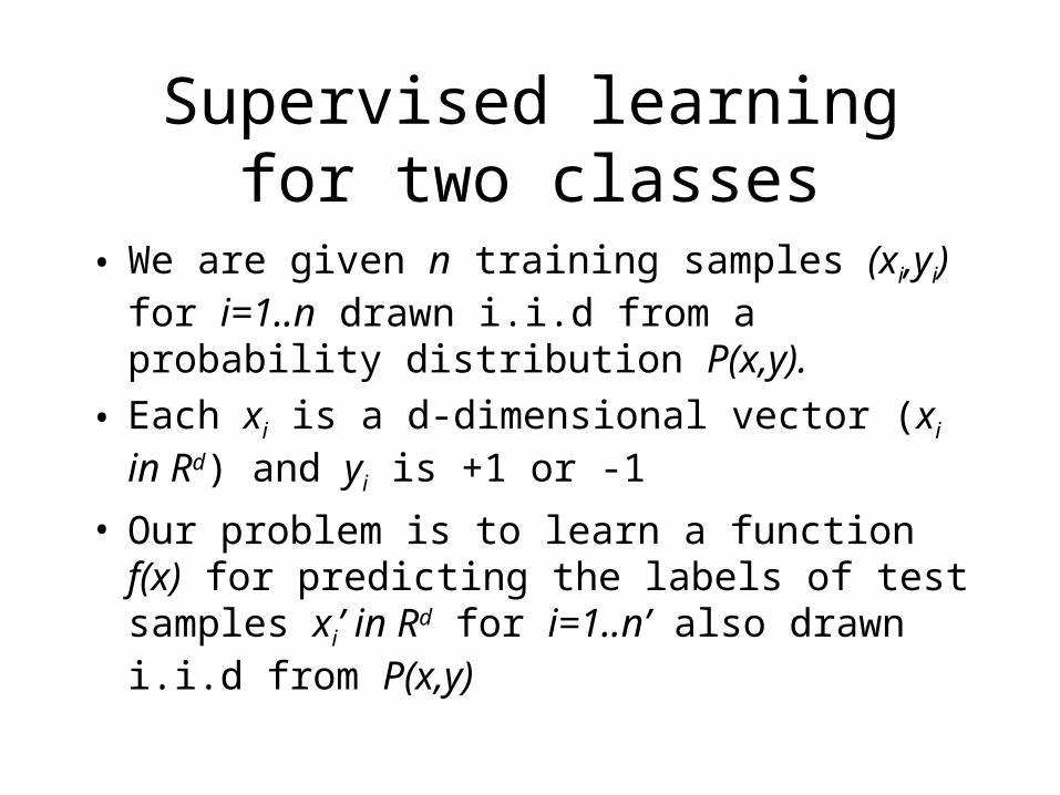
Supervised learning for two classes

• We are given n training samples (xi,yi) for i=1..n drawn i.i.d from a probability distribution P(x,y).

• Each xi is a d-dimensional vector (xi in Rd) and yi is +1 or -1

• Our problem is to learn a function f(x) for predicting the labels of test samples xi’ in Rd for i=1..n’ also drawn i.i.d from P(x,y)

Loss function

• Loss function: c(x,y,f(x))

• Maps to [0,inf]

• Examples:

c(x, y, f (x)) 0 if y f (x)1 otherwise

c(x, y, f (x)) 0 if y f (x)c '(x) otherwise

c(x, y, f (x)) (y f (x))2

Test error

• We quantify the test error as the expected error on the test set (in other words the average test error). In the case of two classes:

• We’d like to find f that minimizes this but we need P(y|x) which we don’t have access to.

Rtest[ f ] 1

n 'c(xi ', y j , f (xi ')

j1

2

)P(y j | xi ')i1

n '

Expected risk

• Suppose we didn’t have test data (x’). Then we average the test error over all possible data points x

• We want to find f that minimizes this but we don’t have all data points. We only have training data.

R[ f ] c(x, y j , f (x)j1

2

)P(y j , x)xX

Empirical risk

• Since we only have training data we can’t calculate the expected risk (we don’t even know P(x,y)).

• Solution: we approximate P(x,y) with the empirical distribution pemp(x,y)

• The delta function δx(y)=1 if x=y and 0 otherwise.

pemp (x, y) 1

n xi (x) yi (y)

i1

n

Empirical risk

• We can now define the empirical risk as

• Once the loss function is defined and training data is given we can then find f that minimizes this.

Remp[ f ] c(x, y j , f (x)j1

2

)pemp (y j , x)xX

1

nc(xi , yi , f (xi )

i1

n

)

Example of minimizing empirical risk (least squares)

• Suppose we are given n data points (xi,yi) where each xi in Rd and yi in R. We want to determine a linear function f(x)=ax+b for predicting test points.

• Loss function c(xi,yi,f(xi))=(yi-f(xi))2

• What is the empirical risk?

Empirical risk for least squares

Remp[ f ] c(xi , yi , f (xi )i1

n

)

(yi f (xi )i1

n

)2

(yi axi b)i1

n

)2

Now finding f has reduced to finding a and b.Since this function is convex in a and b we know thereis a global optimum which is easy to find by settingfirst derivatives to 0.

Maximum likelihood and empirical risk

• Maximizing the likelihood P(D|M) is the same as maximizing log(P(D|M)) which is the same as minimizing -log(P(D|M))

• Set the loss function to

• Now minimizing the empirical risk is the same as maximizing the likelihood

c(xi , yi , f (xi )) log(P(yi | xi , f ))

Empirical risk

• We pose the empirical risk in terms of a loss function and go about to solve it.

• Input: n training samples xi each of dimension d along with labels yi

• Output: a linear function f(x)=wTx+w0 that minimizes the empirical risk

Empirical risk examples

• Linear regression

• How about logistic regression?

1

n(yi f (xi ))

2

i1

n

Logistic regression

• Recall the logistic regression model:

• Let y=+1 be case and y=-1 be control.• The sample likelihood of the training data is

given by

Pr(Dcase |G) 1

1 e (wTGw0 )

Likelihood (1

1 e (wTGi w0 )i1

n _ cases

) (1 1

1 e (wTGi w0 )in _ cases1

n

)

Logistic regression

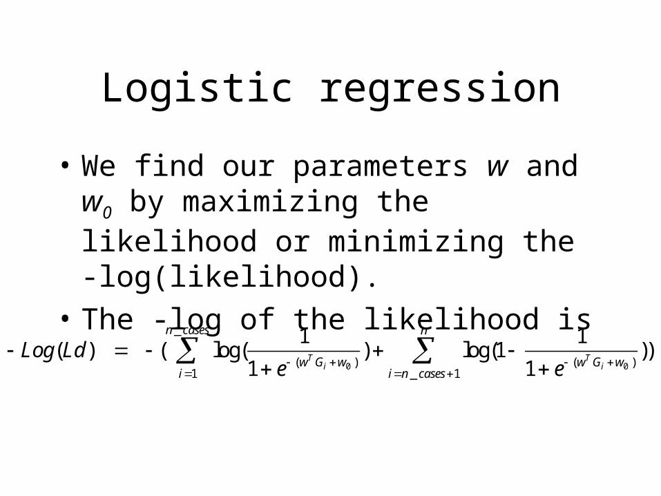
• We find our parameters w and w0 by maximizing the likelihood or minimizing the -log(likelihood).

• The -log of the likelihood is

Log(Ld) ( log(1

1 e (wTGi w0 ))

i1

n _ cases

log(1 1

1 e (wTGi w0 )in _ cases1

n

))

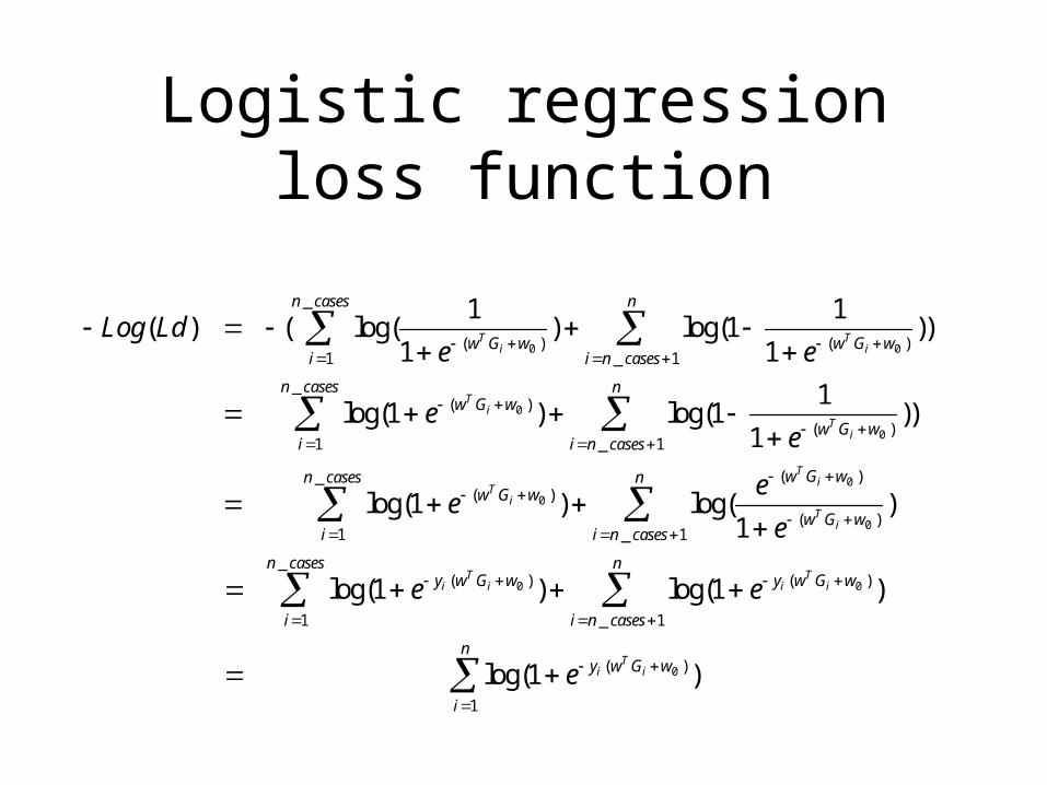
Logistic regression loss function

Log(Ld) ( log(1

1 e (wTGi w0 ))

i1

n _ cases

log(1 1

1 e (wTGi w0 )in _ cases1

n

))

log(1 e (wTGi w0 ) )i1

n _ cases

log(1 1

1 e (wTGi w0 )in _ cases1

n

))

log(1 e (wTGi w0 ) )i1

n _ cases

log(e (wTGi w0 )

1 e (wTGi w0 )in _ cases1

n

)

log(1 e yi (wTGi w0 ) )

i1

n _ cases

log(1 e yi (wTGi w0 )

in _ cases1

n

)

log(1 e yi (wTGi w0 ) )

i1

n

SVM loss function

• Recall the SVM optimization problem:

• The loss function (second term) can be written as

minw,w0 ,i(1

2w

2+C i

i ) subject to yi (w

T xi w0 ) 1 i , for all i

max(0, yi (wT xi w0 )

i1

n

)

Different loss functions

• Linear regression

• Logistic regression

• SVM1

nmax(0, yi (w

T xi w0 )i1

n

)

1

n(yi (wT xi w0 ))2

i1

n

1

nlog(1 e yi (w

TGi w0 ) )i1

n

Regularized risk minimization

• Minimize

• Note the additional term added to the empirical risk.

minimizew (w) Remp (w)

where Remp (w) 1

nl(xi , yi ,w)

i1

n

and (w) w

2 (common setting).

We can use a different norm as well.

Representer theorem

Plays a central role in statistical estimation

Taken from Learning with Kernels by Scholkopf and Smola

Other loss functions

• From “A Scalable Modular Convex Solver for Regularized Risk Minimization”, Teo et. al., KDD 2007

Regularizer

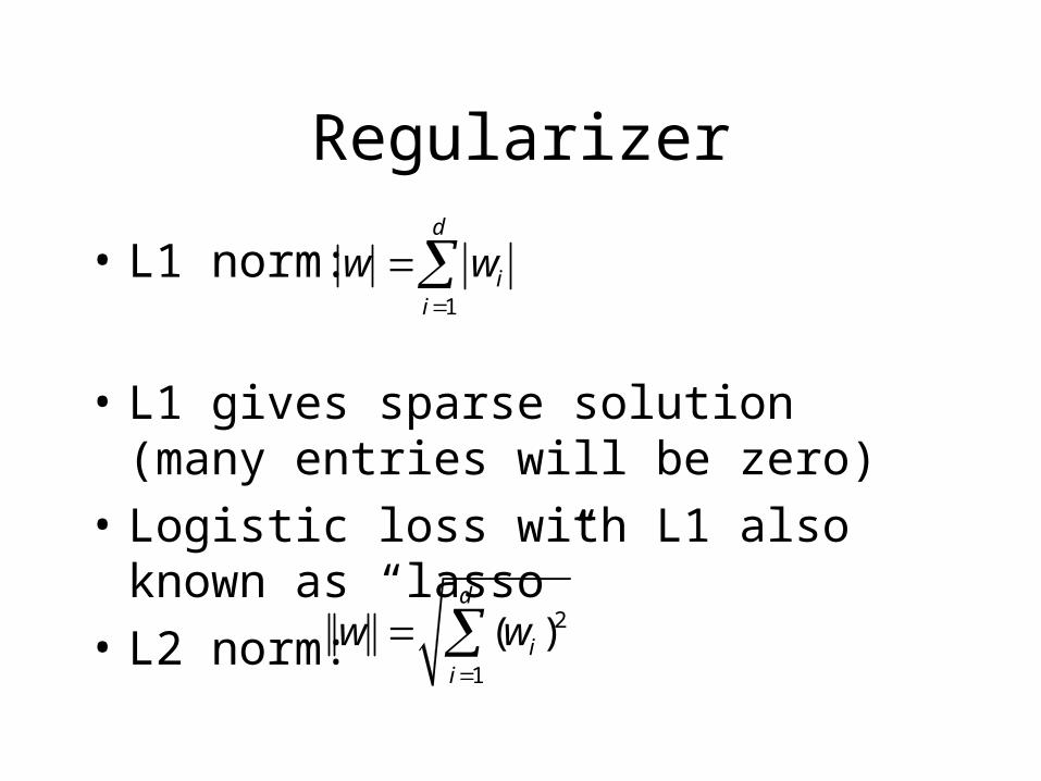
• L1 norm:

• L1 gives sparse solution (many entries will be zero)

• Logistic loss with L1 also known as “lasso”

• L2 norm:

w wii1

d

w (wi )2

i1

d

Regularized risk minimizerexercise

• Compare SVM to regularized logistic regression

• Software: http://users.cecs.anu.edu.au/~chteo/BMRM.html

• Version 2.1 executables for OSL machines available on course website