
Regularization and renormalization - Tata Institute of...
27
Outline Loops EFT End Regularization and renormalization Sourendu Gupta SERC Main School 2014, BITS Pilani Goa, India Effective Field Theories December, 2014 Sourendu Gupta Effective Field Theories 2014: Lecture 2
-
Upload
vuongnguyet -
Category
Documents
-
view
222 -
download
0
Transcript of Regularization and renormalization - Tata Institute of...

Outline Loops EFT End
Regularization and renormalization
Sourendu Gupta
SERC Main School 2014, BITS Pilani Goa, India
Effective Field TheoriesDecember, 2014
Sourendu Gupta Effective Field Theories 2014: Lecture 2

Outline Loops EFT End
Outline
Outline
Spurious divergences in Quantum Field Theory
Wilsonian Effective Field Theories
End matter
Sourendu Gupta Effective Field Theories 2014: Lecture 2

Outline Loops EFT End
Outline
Spurious divergences in Quantum Field Theory
Wilsonian Effective Field Theories
End matter
Sourendu Gupta Effective Field Theories 2014: Lecture 2
Outline Loops EFT End
Outline
Outline
Spurious divergences in Quantum Field Theory
Wilsonian Effective Field Theories
End matter
Sourendu Gupta Effective Field Theories 2014: Lecture 2

Outline Loops EFT End
Perturbation theory: expansion of amplitudes in loops
Any amplitude in a QFT can be expanded in the number of loops.
Sourendu Gupta Effective Field Theories 2014: Lecture 2

Outline Loops EFT End
Perturbation theory: expansion of amplitudes in loops
Born 1 loop 3 loopI=1, V=2 I=4, V=4
2 loop I=7, V=6 I=10, V=8
Any amplitude in a QFT can be expanded in the number of loops.
L = 1 + I − V
Sourendu Gupta Effective Field Theories 2014: Lecture 2

Outline Loops EFT End
Perturbation theory: expansion of amplitudes in loops
Born 1 loop 3 loopI=1, V=2 I=4, V=4
2 loop I=7, V=6 I=10, V=8
Any amplitude in a QFT can be expanded in the number of loops.
L = 1 + I − V
Problem 2.1
Prove the equation. Prove that the expansion in loops is anexpansion in ~, so is a semi-classical expansion. The number ofunconstrained momenta is equal to the number of loops, giving anintegral over each loop momenta. (Hint: See section 6.2 ofQuantum Field Theory , by Itzykson and Zuber.)
Sourendu Gupta Effective Field Theories 2014: Lecture 2

Outline Loops EFT End
Ultraviolet divergences
Typical loop diagrams give rise to integrals of the form
Imn =
∫
d4k
(2π)4k2m
(k2 + ℓ2)n
where k is the loop momentum and ℓ may be some function of theother momenta and the masses. When 2m + 4 ≥ 2n, then theintegral diverges.This can be regularized by putting an UV cutoff, Λ.
Imn =Ω4
(2π)4
∫ Λ
0
k2m+3dk
(k2 + ℓ2)n=
Ω4
(2π)4ℓ2(m−n)+4F
(
Λ
ℓ
)
,
where Ω4 is the result of doing the angular integration. The cutoffmakes this a completely regular integral. As a result, the last partof the answer can be obtained entirely by dimensional analysis.What can we say about the limit Λ → ∞?
Sourendu Gupta Effective Field Theories 2014: Lecture 2

Outline Loops EFT End
Ultraviolet divergences
Typical loop diagrams give rise to integrals of the form
Imn =
∫
d4k
(2π)4k2m
(k2 + ℓ2)n
where k is the loop momentum and ℓ may be some function of theother momenta and the masses. When 2m + 4 ≥ 2n, then theintegral diverges.This can be regularized by putting an UV cutoff, Λ.
Imn =Ω4
(2π)4
∫ Λ
0
k2m+3dk
(k2 + ℓ2)n=
Ω4
(2π)4ℓ2(m−n)+4F
(
Λ
ℓ
)
,
where Ω4 is the result of doing the angular integration. The cutoffmakes this a completely regular integral. As a result, the last partof the answer can be obtained entirely by dimensional analysis.What can we say about the limit Λ → ∞? ???
Sourendu Gupta Effective Field Theories 2014: Lecture 2

Outline Loops EFT End
The old renormalization
We start with a Lagrangian, for example, the 4-Fermi theory:
L =1
2ψ/∂ψ − 1
2mψψ + λ(ψψ)2 + · · ·
Here all the parameters are finite, but the perturbative expansiondiverges, as we saw. We add counter-terms
Lc =1
2Aψ/∂ψ − 1
2Bmψψ + λC (ψψ)2 + · · ·
where A, B , C , etc., are chosen to cancel all divergences inamplitudes. This gives the renormalized Lagrangian
Lr =1
2ψr/∂ψr −
1
2mrψrψr + λr (ψrψr )
2 + · · ·
Clearly, ψr = Zψψ where ψr =√1 + A, mr = m(1 + B)/(1 + A),
λr = λ(1 + C )/(1 + A)2, etc.. The 4-Fermi theory is anunrenormalizable theory since an infinite number of counter-termsare needed to cancel all the divergences arising from L.
Sourendu Gupta Effective Field Theories 2014: Lecture 2

Outline Loops EFT End
Review problems: understanding the old renormalization
Problem 2.2: Self-study
Study the proof of renormalizability of QED to see how one identifies all
the divergences which appear at fixed-loop orders, and how it is shown
that taking care of a fixed number of divergences (through
counter-terms) is sufficient to render the perturbation theory finite. The
curing of the divergence requires fitting a small set of parameters in the
theory to experimental data (a choice of which data is to be fitted is
called a renormalization scheme). As a result, the content of a QFT is to
use some experimental data to predict others.
Problem 2.3
Follow the above steps in a 4-Fermi theory and find a 4-loop diagram
which cannot be regularized using the counter-terms shown in Lc . Would
your arguments also go through for a scalar φ4 theory? Unrenormalizable
theories require infinite amount of input data.
Sourendu Gupta Effective Field Theories 2014: Lecture 2

Outline Loops EFT End
Dimensional regularization
The UV divergences we are worried about can be cured if D < 4.So, instead of the four-dimensional integral, try to perform anintegral in 4 + δ dimensions, and then take the limit δ → 0−. Sinceeverything is to be defined by analytic continuation, we will notworry about the sign of δ until the end.
The integrals of interest are
Imn =
∫
d4k
(2π)4k2m
(k2 + ℓ2)n→
∫
d4+δk
µδ(2π)4+δ(k2δ + k2)m
(k2δ + k2 + ℓ2)n,
where we have introduced an arbitrary mass scale, µ, in the secondform of the integral in order to keep the dimension of Inunchanged. Also, the square of the 4 + δ dimensional momentum,k , has been decomposed into its four dimensional part, k2, and theremainder, k2δ .
Sourendu Gupta Effective Field Theories 2014: Lecture 2

Outline Loops EFT End
Doing the integral in one step
Usually one does the integral in 4 + δ dimensions in one step:
Imn = µ4−D
∫
dDk
(2π)Dk2m
(k2 + ℓ2)n
= ℓ2m+4−2n
(
ℓ
µ
)D−4 ΩD
(2π)DΓ(m + D/2)Γ(n −m − D/2)
2Γ(n),
where ΩD = Γ(D/2)/(2π)D/2 is the volume of an unit sphere in D
dimensions.
For m = 0 and n = 1, setting D = 4− 2ǫ, the ǫ-dependent termsbecome
(
ℓ2
4πµ2
)
−ǫ
Γ(−1 + ǫ) = −1
ǫ+ γ − 1 + log
[
ℓ2
4πµ2
]
+O(ǫ),
where γ is the Euler-Mascheroni constant.Sourendu Gupta Effective Field Theories 2014: Lecture 2

Outline Loops EFT End
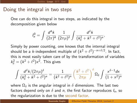
Doing the integral in two steps
One can do this integral in two steps, as indicated by thedecomposition given below
I 0n =
∫
d4k
(2π)41
(2πµ)δ
∫
dδk
(k2δ + k2 + ℓ2)n,
Simply by power counting, one knows that the internal integralshould be a k-independent multiple of (k2 + ℓ2)−n+δ/2. In fact,this is most easily taken care of by the transformation of variablesk2δ = (k2 + ℓ2)x2. This gives
∫
dδk/(2πµ)δ
(k2δ + k2 + ℓ2)n=
1
(k2 + ℓ2)n
(
k2 + ℓ2
2πµ
)δ
Ωδ
∫
xδ−1dx
(1 + x2)n
where Ωδ is the angular integral in δ dimensions. The last twofactors depend only on δ and n, the first factor reproduces In, sothe regularization is due to the second factor.
Sourendu Gupta Effective Field Theories 2014: Lecture 2
Outline Loops EFT End
Doing the integral in two steps
One can do this integral in two steps, as indicated by thedecomposition given below
I 0n =
∫
d4k
(2π)41
(2πµ)δ
∫
dδk
(k2δ + k2 + ℓ2)n,
Simply by power counting, one knows that the internal integralshould be a k-independent multiple of (k2 + ℓ2)−n+δ/2. In fact,this is most easily taken care of by the transformation of variablesk2δ = (k2 + ℓ2)x2. This gives
∫
dδk/(2πµ)δ
(k2δ + k2 + ℓ2)n=
1
(k2 + ℓ2)n
(
k2 + ℓ2
2πµ
)δ
Ωδ
∫
xδ−1dx
(1 + x2)n
where Ωδ is the angular integral in δ dimensions. The last twofactors depend only on δ and n, the first factor reproduces In, sothe regularization is due to the second factor.
Sourendu Gupta Effective Field Theories 2014: Lecture 2

Outline Loops EFT End
Recognizing the regularization
The regulation becomes transparent by writing
(
k2 + ℓ2
2πµ
)δ
= exp
[
δ log
(
k2 + ℓ2
2πµ
)]
.
For fixed µ, the logarithm goes to a constant when k → 0. Also,the logarithm goes to −∞ when k → ∞. As a result, theregulating factor goes to zero provided δ < 0. This is exactly theintuition we started from.
In the context of dimensional regularization, the quantity µ iscalled the renormalization scale. We have seen that it gives anultraviolet cutoff. The important thing is that the scale µ iscompletely arbitrary, and has nothing to do with the range ofapplicability of the QFT.
Sourendu Gupta Effective Field Theories 2014: Lecture 2

Outline Loops EFT End
Outline
Outline
Spurious divergences in Quantum Field Theory
Wilsonian Effective Field Theories
End matter
Sourendu Gupta Effective Field Theories 2014: Lecture 2

Outline Loops EFT End
The old renormalization
In 1929, Heisenberg and Pauli wrote down a general formulationfor QFT and noted the problem of infinities in using perturbationtheory. After 1947 the problem was considered solved. The generaloutline of the method is the following:
Analyze perturbation theory for the loop integrals which haveultraviolet divergences.
Regulate these divergences by putting an ultraviolet cutoff insome consistent way.
Identify the independent sources of divergences, and add tothe Lagrangian counter-terms which precisely cancel thesedivergences.
QFTs are called renormalizable if there are a finite number ofcounter-terms needed to render perturbation theory useful.
Use only renormalizable Lagrangians as models for physicalphenomena.
Sourendu Gupta Effective Field Theories 2014: Lecture 2

Outline Loops EFT End
Unrenormalizable terms
In this view, the unrenormalizable Lagrangian
Lint = −λ(ψψ)2,was deemed impossible as a model for physical phenomena, since itneeds an infinite number of counter-terms.
q
k k
Examine its contribution to the fermion mass:
imλ
∫
d4q
(2π)41
q2 −m2∝ λmΛ2,
where the integral is regulated by cutting it off at the scale Λ. Athigher loop orders the dependence on Λ would be even stronger. Inthe modern view, this analysis is mistaken because it confuses twodifferent things.
Sourendu Gupta Effective Field Theories 2014: Lecture 2

Outline Loops EFT End
Unrenormalizable terms
In this view, the unrenormalizable Lagrangian
Lint = −λ(ψψ)2,was deemed impossible as a model for physical phenomena, since itneeds an infinite number of counter-terms.
q
k k
k k
+ 1 − log(4 )γ1ε − π
Examine its contribution to the fermion mass:
imλ
∫
d4q
(2π)41
q2 −m2∝ λmΛ2,
where the integral is regulated by cutting it off at the scale Λ. Athigher loop orders the dependence on Λ would be even stronger. Inthe modern view, this analysis is mistaken because it confuses twodifferent things.
Sourendu Gupta Effective Field Theories 2014: Lecture 2

Outline Loops EFT End
Irrelevant terms
Today the same Lagrangian is written as
Lint = − λ
Λ2(ψψ)2,
where Λ is interpreted as a scale below which one should apply thetheory.The contribution to the mass is
imλ
Λ2
∫
d4q
(2π)41
q2 −m2=
m3
16π2Λ2
(
−1
ǫ+ γ − 1 + log
[
m2
4πµ2
])
,
where the integral regulated by doing it in 4− 2ǫ dimensions. Inthe MS renormalization scheme the counter-term subtracts thepole and the finite parts γ − 1− log 4π, leaving
δm
m=
λ
16π2
(m
Λ
)2log
[
m2
µ2
]
.
Sourendu Gupta Effective Field Theories 2014: Lecture 2

Outline Loops EFT End
Separation of scales
The cutoff scale in the problem, Λ, is dissociated from therenormalization scale, µ, in dimensional regularization. This is nottrue in cutoff regularization. This separation of scales allows us torecognize two things:
There is no divergence in the limit Λ → ∞; instead thecoupling becomes irrelevant. The theory remains predictive,because the effect of these terms is bounded.
There are no large logarithms such as log(m/Λ). Theamplitudes, computed to all orders are independent of µ,although fixed loop orders are not. In practical fixedloop-order computations, it is possible to choose µ ≃ m, andreduce the dependence on this spurious scale.
Regularization schemes which do this are called mass-independentregularization. They are a crucial technical step in the newWilsonian way of thinking about renormalization.
Sourendu Gupta Effective Field Theories 2014: Lecture 2

Outline Loops EFT End
Is cutoff regularization wrong?
All regularizations must give the same results when theperturbation theory is done to all orders. Cutoff regularization isjust more cumbersome.
Cutoff regularization retains all the problems of the old view: sincethe cutoff and renormalization scales are not separated, higherdimensional counter-terms are needed to cancel the worseningdivergences at higher loop orders. When all is computed andcancelled, the m2/Λ2 and log(m/Λ) emerge.
In mass-independent regularization schemes, higher dimensionalterms give smaller corrections because of larger powers of m/Λ.
In a renormalizable theory, since the number of counter-terms isfinite and small, the equivalence of different regularizations iseasier to see.
Sourendu Gupta Effective Field Theories 2014: Lecture 2

Outline Loops EFT End
Chiral symmetry: an important secondary issue
In this example we find that δm ∝ m; if the bare mass were zero,then the renormalized mass remains zero. There is a symmetryreason behind this.
A Dirac spinor can be resolved into left and right handedcomponents using the projection operators 1± γ5. The twocomponents are decoupled in the kinetic term, but coupled by themass term. In the absence of the mass term at the tree level, thetheory has chiral symmetry: ψ → γ5ψ.
If chiral symmetry is not broken by Lint, then the massrenormalization must vanish as m → 0. Chiral Ward identities cansay which terms in Lint are allowed by chiral symmetry.
Sourendu Gupta Effective Field Theories 2014: Lecture 2
Outline Loops EFT End
Outline
Outline
Spurious divergences in Quantum Field Theory
Wilsonian Effective Field Theories
End matter
Sourendu Gupta Effective Field Theories 2014: Lecture 2

Outline Loops EFT End
Keywords and References
Keywords
Loop integrals; ultraviolet cutoff scale; cutoff regularization; largelogarithms; dimensional regularization; mass-independentregularization; counter-terms; renormalization scheme;renormalization scale; msbar renormalization scheme;un-renormalizable theory; renormalizable Lagrangians;super-renormalizable couplings; Chiral Ward identities;
References
David B. Kaplan, Effective Field Theories, arxiv: nucl-th/9506035;Aneesh Manohar, Effective Field Theories, arxiv: hep-ph/9606222;S. Weinberg, The Quantum Theory of Fields Vol II.
Sourendu Gupta Effective Field Theories 2014: Lecture 2

Outline Loops EFT End
Copyright statement
Copyright for this work remains with Sourendu Gupta. However,teachers are free to use them in this form in classrooms withoutchanging the author’s name or this copyright statement. They arefree to paraphrase or extract material for legitimate classroom oracademic use with the usual academic fair use conventions.
If you are a teacher and use this material in your classes, I wouldbe very happy to hear of your experience. I will also be very happyif you write to me to point out errors.
This material may not be sold or exchanged for service, orincorporated into other media which is sold or exchanged forservice. This material may not be distributed on any other websiteexcept by my written permission.
Sourendu Gupta Effective Field Theories 2014: Lecture 2


![Wonderful Renormalization - Institut für Mathematikkreimer/wp-content/uploads/Berghoff... · Wonderful Renormalization ... [FM94], serve as a ... inition of the wonderful renormalization](https://static.fdocuments.us/doc/165x107/5aefc8817f8b9a8b4c8cb959/wonderful-renormalization-institut-fr-kreimerwp-contentuploadsberghoffwonderful.jpg)
