
Regression Models for Ordinal and Nominal Dependent Variables
76
I n d i a n a U n i v e r s i t y University Information Technology Services Regression Models for Ordinal and Nominal Dependent Variables Using SAS, Stata, LIMDEP, and SPSS * Hun Myoung Park, Ph.D. © 2003-2009 Last modified on September 2009 University Information Technology Services Center for Statistical and Mathematical Computing Indiana University 410 North Park Avenue Bloomington, IN 47408 (812) 855-4724 (317) 278-4740 http://www.indiana.edu/~statmath * The citation of this document should read: “Park, Hun Myoung. 2009. Regression Models for Ordinal and Nominal Dependent Variables Using SAS, Stata, LIMDEP, and SPSS. Working Paper. The University Information Technology Services (UITS) Center for Statistical and Mathematical Computing, Indiana University.” http://www.indiana.edu/~statmath/stat/all/cdvm/index_nomial.html
Transcript of Regression Models for Ordinal and Nominal Dependent Variables
I n d i a n a U n i v e r s i t y U n i v e r s i t y I n f o r m a t i o n T e c h n o l o g y S e r v i c e s
Regression Models for Ordinal and Nominal Dependent Variables Using SAS, Stata, LIMDEP, and SPSS*
Hun Myoung Park, Ph.D.
© 2003-2009 Last modified on September 2009
University Information Technology Services Center for Statistical and Mathematical Computing
Indiana University 410 North Park Avenue Bloomington, IN 47408
(812) 855-4724 (317) 278-4740 http://www.indiana.edu/~statmath
* The citation of this document should read: “Park, Hun Myoung. 2009. Regression Models for Ordinal and Nominal Dependent Variables Using SAS, Stata, LIMDEP, and SPSS. Working Paper. The University Information Technology Services (UITS) Center for Statistical and Mathematical Computing, Indiana University.” http://www.indiana.edu/~statmath/stat/all/cdvm/index_nomial.html
© 2003-2009, The Trustees of Indiana University Regression Models for Ordinal and Nominal DVs: 2
http://www.indiana.edu/~statmath 2
This document summarizes logit and probit regression models for ordinal and nominal dependent variables and illustrates how to estimate individual models using SAS 9.2, Stata 11, LIMDEP 9, and SPSS 17. 1. Introduction 2. Ordinal Logit and Probit Models 3. Multinomial Logit Model 4. Conditional Logit Model 5. Nested Logit Model 6. Conclusion References
1. Introduction
A categorical variable here refers to a variable that is binary, ordinal, or nominal. Event count data are discrete (categorical) but often treated as continuous variables. When a dependent variable is categorical, the ordinary least squares (OLS) method can no longer produce the best linear unbiased estimator (BLUE); that is, OLS is biased and inefficient. Consequently, researchers have developed various regression models for categorical dependent variables. The nonlinearity of categorical dependent variable models makes it difficult to fit the models and interpret their results. 1.1 Regression Models for Categorical Dependent Variables In categorical dependent variable models, the left-hand side (LHS) variable or dependent variable is neither interval nor ratio, but rather categorical. The level of measurement and data generation process (DGP) of a dependent variable determine a proper model for data analysis. Binary responses (0 or 1) are modeled with binary logit and probit regressions, ordinal responses (1st, 2nd, 3rd, …) are formulated into (generalized) ordinal logit/probit regressions, and nominal responses are analyzed by the multinomial logit (probit), conditional logit, or nested logit model depending on specific circumstances. Independent variables on the right-hand side (RHS) are interval, ratio, and/or binary (dummy). Table 1.1 Ordinary Least Squares and Categorical Dependent Variable Models Model Dependent (LHS) Estimation Independent (RHS)
OLS Ordinary least squares
Interval or ratio Moment based method
Binary response Binary (0 or 1)
Ordinal response Ordinal (1st, 2nd , 3rd…) Nominal response Nominal (A, B, C …)
Categorical DV Models
Event count data Count (0, 1, 2, 3…)
Maximum likelihood method
A linear function of interval/ratio or binary variables
...22110 XX
Categorical dependent variable models adopt the maximum likelihood (ML) estimation method, whereas OLS uses the moment based method. The ML method requires an assumption about probability distribution functions, such as the logistic function and the complementary log-log
© 2003-2009, The Trustees of Indiana University Regression Models for Ordinal and Nominal DVs: 3
http://www.indiana.edu/~statmath 3
function. Logit models use the standard logistic probability distribution, while probit models assume the standard normal distribution. This document focuses on logit and probit models only, excluding regression models for event count data (e.g., negative binomial regression model and zero-inflated or zero-truncated regression models). Table 1.1 summarizes categorical dependent variable models in comparison with OLS. 1.2 Logit Models versus Probit Models How do logit models differ from probit models? The core difference lies in the distribution of errors (disturbances). In the logit model, errors are assumed to follow the standard logistic
distribution with mean 0 and variance 3
2, 2)1(
)(
e
e
. The errors of the probit model are
assumed to follow the standard normal distribution, 2
2
2
1)(
e with variance 1.
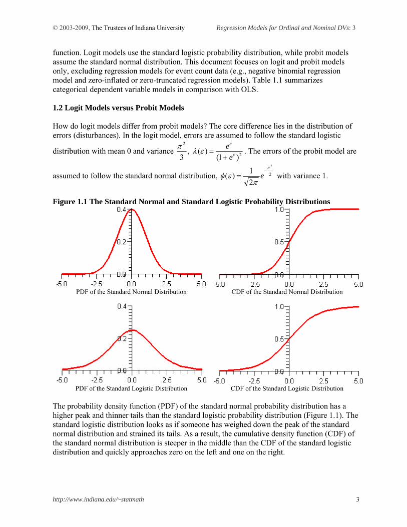
Figure 1.1 The Standard Normal and Standard Logistic Probability Distributions
PDF of the Standard Normal Distribution CDF of the Standard Normal Distribution
PDF of the Standard Logistic Distribution CDF of the Standard Logistic Distribution The probability density function (PDF) of the standard normal probability distribution has a higher peak and thinner tails than the standard logistic probability distribution (Figure 1.1). The standard logistic distribution looks as if someone has weighed down the peak of the standard normal distribution and strained its tails. As a result, the cumulative density function (CDF) of the standard normal distribution is steeper in the middle than the CDF of the standard logistic distribution and quickly approaches zero on the left and one on the right.
© 2003-2009, The Trustees of Indiana University Regression Models for Ordinal and Nominal DVs: 4
http://www.indiana.edu/~statmath 4
The two models, of course, produce different parameter estimates. In binary response models,
the estimates of a logit model are roughly 3 times larger than those of the probit model. These estimators, however, end up with almost the same standardized impacts of independent variables (Long 1997). The choice between logit and probit models is more closely related to estimation and familiarity rather than theoretical and interpretive aspects. In general, logit models reach convergence fairly well. Although some (multinomial) probit models may take a long time to reach convergence, a probit model works well for bivariate models. As computing power improves and new algorithms are developed, importance of this issue is diminishing. For discussion on choosing logit and probit models, see Cameron and Trivedi (2009: 471-474).
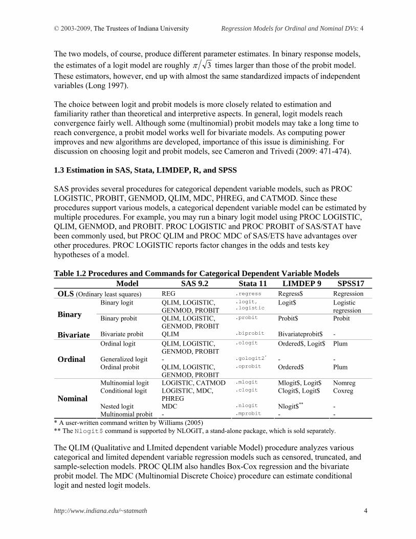
1.3 Estimation in SAS, Stata, LIMDEP, R, and SPSS SAS provides several procedures for categorical dependent variable models, such as PROC LOGISTIC, PROBIT, GENMOD, QLIM, MDC, PHREG, and CATMOD. Since these procedures support various models, a categorical dependent variable model can be estimated by multiple procedures. For example, you may run a binary logit model using PROC LOGISTIC, QLIM, GENMOD, and PROBIT. PROC LOGISTIC and PROC PROBIT of SAS/STAT have been commonly used, but PROC QLIM and PROC MDC of SAS/ETS have advantages over other procedures. PROC LOGISTIC reports factor changes in the odds and tests key hypotheses of a model. Table 1.2 Procedures and Commands for Categorical Dependent Variable Models
Model SAS 9.2 Stata 11 LIMDEP 9 SPSS17 OLS (Ordinary least squares) REG .regress Regress$ Regression
Binary logit QLIM, LOGISTIC, GENMOD, PROBIT
.logit,
.logistic Logit$ Logistic
regression Binary Binary probit QLIM, LOGISTIC, GENMOD, PROBIT
.probit Probit$ Probit
Bivariate Bivariate probit QLIM .biprobit Bivariateprobit$ -
Ordinal logit QLIM, LOGISTIC, GENMOD, PROBIT
.ologit Ordered$, Logit$ Plum
Generalized logit - .gologit2* - - Ordinal Ordinal probit QLIM, LOGISTIC,
GENMOD, PROBIT .oprobit Ordered$ Plum
Multinomial logit LOGISTIC, CATMOD .mlogit Mlogit$, Logit$ Nomreg Conditional logit LOGISTIC, MDC,
PHREG .clogit Clogit$, Logit$ Coxreg
Nested logit MDC .nlogit Nlogit$** - Nominal
Multinomial probit - .mprobit - - * A user-written command written by Williams (2005) ** The Nlogit$ command is supported by NLOGIT, a stand-alone package, which is sold separately. The QLIM (Qualitative and LImited dependent variable Model) procedure analyzes various categorical and limited dependent variable regression models such as censored, truncated, and sample-selection models. PROC QLIM also handles Box-Cox regression and the bivariate probit model. The MDC (Multinomial Discrete Choice) procedure can estimate conditional logit and nested logit models.
© 2003-2009, The Trustees of Indiana University Regression Models for Ordinal and Nominal DVs: 5
http://www.indiana.edu/~statmath 5
Another advantage of using SAS is the Output Delivery System (ODS), which makes it easy to manage SAS output. ODS enables users to redirect the output to HTML (Hypertext Markup Language) and RTF (Rich Text Format) formats. Once SAS output is generated in a HTML document, users can easily handle tables and graphics especially when copying and pasting them into a wordprocessor document. Unlike SAS, Stata has individualized commands for corresponding categorical dependent variable models. For example, the .logit and .probit commands respectively fit the binary logit and probit models, while .mlogit and .nlogit estimate the mulitinomial logit and nested logit models. Stata enables users to perform post-hoc analyses such as marginal effects and discrete changes in an easy manner. The LIMDEP Logit$ and Probit$ commands support a variety of categorical dependent variable models that are addressed in Greene’s Econometric Analysis (2003). The output format of LIMDEP 9 is slightly different from that of previous version, but key statistics remain unchanged. The nested logit model and multinomial probit model in LIMDEP are estimated by NLOGIT, a separate package. In R, glm() fits binary logit and probit models in the object- oriented programming concept. SPSS also supports some categorical dependent variable models and its output is often messy and hard to read. Stata and R are case-sensitive, but SAS, LIMDEP, and SPSS are not. Table 1.2 summarizes the procedures and commands used for categorical dependent variable models. 1. 4 Long and Freese’s SPost Stata users may benefit from user-written commands such as J. Scott Long and Jeremy Freese’s SPost. This collection of user-written commands conducts many follow-up analyses of various categorical dependent variable models including event count data models (See section 2.2). In order to install SPost, execute the following commands consecutively. Visit J. Scott Long’s Web site at http://www.indiana.edu/~jslsoc/ to get further information. . net from http://www.indiana.edu/~jslsoc/stata/ . net install spost9_ado, replace . net get spost9_do, replace
If a Stata command, function, or user-written command does not work in version 11, run the .version command to switch the interpreter to old one and execute that command again. For example, normal() was norm() in old versions. Also you may update Stata or reinstall user-written models to get their latest version installed. . version 9
You may use Vincent Kang Fu’s gologit (1998) and Richard Williams’ gologit2 (2005) for the generalized ordinal logit model. .mfx2 is a related command written by Williams to compute marginal effects (discrete changes) in (generalized) ordinal logit and multinomial logit models. Visit http://www.nd.edu/~rwilliam/gologit2/tsfaq.html for more information. . net install gologit, from(http://www.stata.com/users/jhardin) replace . ssc install gologit2, replace . ssc install mfx2, replace
© 2003-2009, The Trustees of Indiana University Regression Models for Ordinal and Nominal DVs: 6
http://www.indiana.edu/~statmath 6
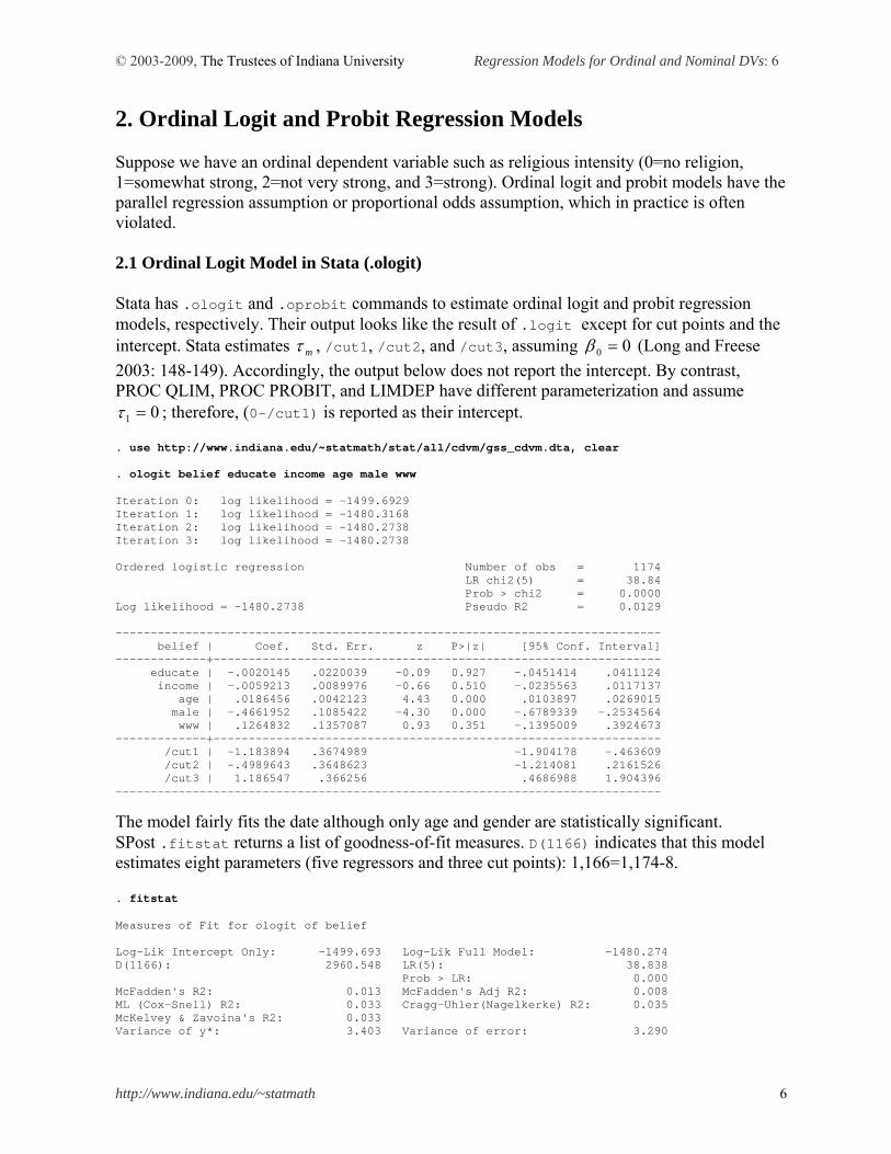
2. Ordinal Logit and Probit Regression Models Suppose we have an ordinal dependent variable such as religious intensity (0=no religion, 1=somewhat strong, 2=not very strong, and 3=strong). Ordinal logit and probit models have the parallel regression assumption or proportional odds assumption, which in practice is often violated. 2.1 Ordinal Logit Model in Stata (.ologit) Stata has .ologit and .oprobit commands to estimate ordinal logit and probit regression models, respectively. Their output looks like the result of .logit except for cut points and the intercept. Stata estimates m , /cut1, /cut2, and /cut3, assuming 00 (Long and Freese
2003: 148-149). Accordingly, the output below does not report the intercept. By contrast, PROC QLIM, PROC PROBIT, and LIMDEP have different parameterization and assume
01 ; therefore, (0-/cut1) is reported as their intercept. . use http://www.indiana.edu/~statmath/stat/all/cdvm/gss_cdvm.dta, clear . ologit belief educate income age male www Iteration 0: log likelihood = -1499.6929 Iteration 1: log likelihood = -1480.3168 Iteration 2: log likelihood = -1480.2738 Iteration 3: log likelihood = -1480.2738 Ordered logistic regression Number of obs = 1174 LR chi2(5) = 38.84 Prob > chi2 = 0.0000 Log likelihood = -1480.2738 Pseudo R2 = 0.0129 ------------------------------------------------------------------------------ belief | Coef. Std. Err. z P>|z| [95% Conf. Interval] -------------+---------------------------------------------------------------- educate | -.0020145 .0220039 -0.09 0.927 -.0451414 .0411124 income | -.0059213 .0089976 -0.66 0.510 -.0235563 .0117137 age | .0186456 .0042123 4.43 0.000 .0103897 .0269015 male | -.4661952 .1085422 -4.30 0.000 -.6789339 -.2534564 www | .1264832 .1357087 0.93 0.351 -.1395009 .3924673 -------------+---------------------------------------------------------------- /cut1 | -1.183894 .3674989 -1.904178 -.463609 /cut2 | -.4989643 .3648623 -1.214081 .2161526 /cut3 | 1.186547 .366256 .4686988 1.904396 ------------------------------------------------------------------------------
The model fairly fits the date although only age and gender are statistically significant. SPost .fitstat returns a list of goodness-of-fit measures. D(1166) indicates that this model estimates eight parameters (five regressors and three cut points): 1,166=1,174-8. . fitstat Measures of Fit for ologit of belief Log-Lik Intercept Only: -1499.693 Log-Lik Full Model: -1480.274 D(1166): 2960.548 LR(5): 38.838 Prob > LR: 0.000 McFadden's R2: 0.013 McFadden's Adj R2: 0.008 ML (Cox-Snell) R2: 0.033 Cragg-Uhler(Nagelkerke) R2: 0.035 McKelvey & Zavoina's R2: 0.033 Variance of y*: 3.403 Variance of error: 3.290
© 2003-2009, The Trustees of Indiana University Regression Models for Ordinal and Nominal DVs: 7
http://www.indiana.edu/~statmath 7
Count R2: 0.407 Adj Count R2: 0.031 AIC: 2.535 AIC*n: 2976.548 BIC: -5280.941 BIC': -3.497 BIC used by Stata: 3017.093 AIC used by Stata: 2976.548
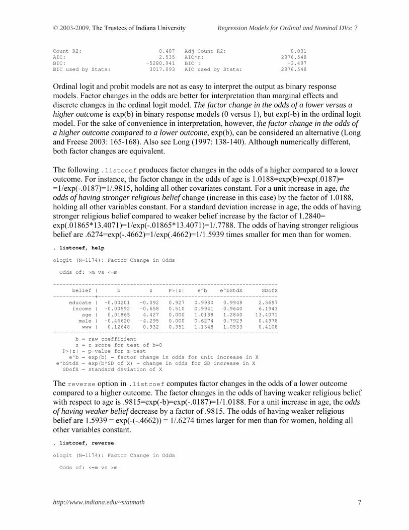
Ordinal logit and probit models are not as easy to interpret the output as binary response models. Factor changes in the odds are better for interpretation than marginal effects and discrete changes in the ordinal logit model. The factor change in the odds of a lower versus a higher outcome is exp(b) in binary response models (0 versus 1), but exp(-b) in the ordinal logit model. For the sake of convenience in interpretation, however, the factor change in the odds of a higher outcome compared to a lower outcome, exp(b), can be considered an alternative (Long and Freese 2003: 165-168). Also see Long (1997: 138-140). Although numerically different, both factor changes are equivalent. The following .listcoef produces factor changes in the odds of a higher compared to a lower outcome. For instance, the factor change in the odds of age is 1.0188=exp(b)=exp(.0187)= =1/exp(-.0187)=1/.9815, holding all other covariates constant. For a unit increase in age, the odds of having stronger religious belief change (increase in this case) by the factor of 1.0188, holding all other variables constant. For a standard deviation increase in age, the odds of having stronger religious belief compared to weaker belief increase by the factor of 1.2840= exp(.01865*13.4071)=1/exp(-.01865*13.4071)=1/.7788. The odds of having stronger religious belief are .6274=exp(-.4662)=1/exp(.4662)=1/1.5939 times smaller for men than for women. . listcoef, help ologit (N=1174): Factor Change in Odds Odds of: >m vs <=m ---------------------------------------------------------------------- belief | b z P>|z| e^b e^bStdX SDofX -------------+-------------------------------------------------------- educate | -0.00201 -0.092 0.927 0.9980 0.9948 2.5697 income | -0.00592 -0.658 0.510 0.9941 0.9640 6.1943 age | 0.01865 4.427 0.000 1.0188 1.2840 13.4071 male | -0.46620 -4.295 0.000 0.6274 0.7929 0.4978 www | 0.12648 0.932 0.351 1.1348 1.0533 0.4108 ---------------------------------------------------------------------- b = raw coefficient z = z-score for test of b=0 P>|z| = p-value for z-test e^b = exp(b) = factor change in odds for unit increase in X e^bStdX = exp(b*SD of X) = change in odds for SD increase in X SDofX = standard deviation of X
The reverse option in .listcoef computes factor changes in the odds of a lower outcome compared to a higher outcome. The factor changes in the odds of having weaker religious belief with respect to age is .9815=exp(-b)=exp(-.0187)=1/1.0188. For a unit increase in age, the odds of having weaker belief decrease by a factor of .9815. The odds of having weaker religious belief are 1.5939 = exp(-(-.4662)) = 1/.6274 times larger for men than for women, holding all other variables constant. . listcoef, reverse ologit (N=1174): Factor Change in Odds Odds of: <=m vs >m
© 2003-2009, The Trustees of Indiana University Regression Models for Ordinal and Nominal DVs: 8
http://www.indiana.edu/~statmath 8
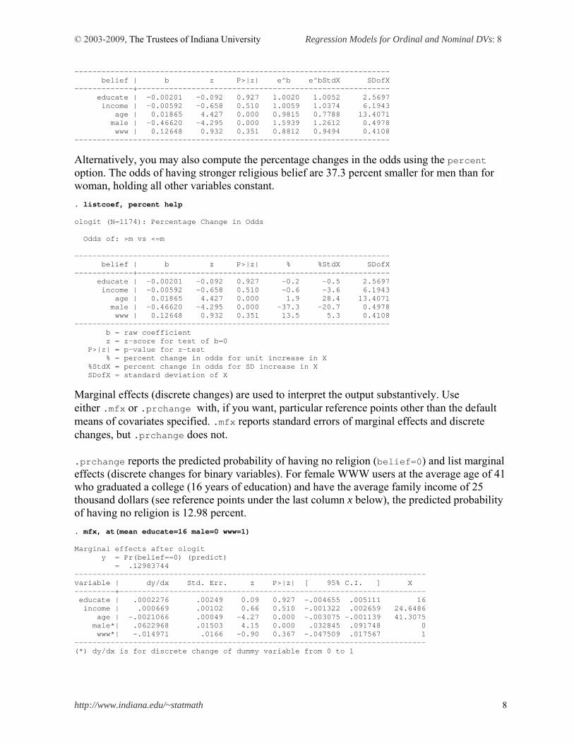
---------------------------------------------------------------------- belief | b z P>|z| e^b e^bStdX SDofX -------------+-------------------------------------------------------- educate | -0.00201 -0.092 0.927 1.0020 1.0052 2.5697 income | -0.00592 -0.658 0.510 1.0059 1.0374 6.1943 age | 0.01865 4.427 0.000 0.9815 0.7788 13.4071 male | -0.46620 -4.295 0.000 1.5939 1.2612 0.4978 www | 0.12648 0.932 0.351 0.8812 0.9494 0.4108 ----------------------------------------------------------------------
Alternatively, you may also compute the percentage changes in the odds using the percent option. The odds of having stronger religious belief are 37.3 percent smaller for men than for woman, holding all other variables constant. . listcoef, percent help ologit (N=1174): Percentage Change in Odds Odds of: >m vs <=m ---------------------------------------------------------------------- belief | b z P>|z| % %StdX SDofX -------------+-------------------------------------------------------- educate | -0.00201 -0.092 0.927 -0.2 -0.5 2.5697 income | -0.00592 -0.658 0.510 -0.6 -3.6 6.1943 age | 0.01865 4.427 0.000 1.9 28.4 13.4071 male | -0.46620 -4.295 0.000 -37.3 -20.7 0.4978 www | 0.12648 0.932 0.351 13.5 5.3 0.4108 ---------------------------------------------------------------------- b = raw coefficient z = z-score for test of b=0 P>|z| = p-value for z-test % = percent change in odds for unit increase in X %StdX = percent change in odds for SD increase in X SDofX = standard deviation of X
Marginal effects (discrete changes) are used to interpret the output substantively. Use either .mfx or .prchange with, if you want, particular reference points other than the default means of covariates specified. .mfx reports standard errors of marginal effects and discrete changes, but .prchange does not. .prchange reports the predicted probability of having no religion (belief=0) and list marginal effects (discrete changes for binary variables). For female WWW users at the average age of 41 who graduated a college (16 years of education) and have the average family income of 25 thousand dollars (see reference points under the last column x below), the predicted probability of having no religion is 12.98 percent. . mfx, at(mean educate=16 male=0 www=1) Marginal effects after ologit y = Pr(belief==0) (predict) = .12983744 ------------------------------------------------------------------------------ variable | dy/dx Std. Err. z P>|z| [ 95% C.I. ] X ---------+-------------------------------------------------------------------- educate | .0002276 .00249 0.09 0.927 -.004655 .005111 16 income | .000669 .00102 0.66 0.510 -.001322 .002659 24.6486 age | -.0021066 .00049 -4.27 0.000 -.003075 -.001139 41.3075 male*| .0622968 .01503 4.15 0.000 .032845 .091748 0 www*| -.014971 .0166 -0.90 0.367 -.047509 .017567 1 ------------------------------------------------------------------------------ (*) dy/dx is for discrete change of dummy variable from 0 to 1

© 2003-2009, The Trustees of Indiana University Regression Models for Ordinal and Nominal DVs: 9
http://www.indiana.edu/~statmath 9
Marginal effects and discrete changes are more intuitive than factor changes in the odds. For 10 unit increase in age from its mean 41, the probability of having no religion is expected to decrease by 2.1 percent (.21*10), holding all other variables constant at the reference points. Men are 6.23 percent more likely than women to have no religion at the same reference points.
.prchange reports predicted probabilities of four religious intensity and produces marginal effects (-+1/2 or MargEfct) and discrete changes (0->1) of covariates in probabilities of all four outcomes. This command computes marginal effects for a standard deviation change (-+sd/2) as well. . prchange age male, x(educate=16 male=0 www=1) rest(mean) ologit: Changes in Probabilities for belief age Avg|Chg| No_relig Somewhat Not_very Strong Min->Max .1509029 -.12637663 -.07334894 -.10208026 .30180579 -+1/2 .00220756 -.00210658 -.00117922 -.00112933 .00441512 -+sd/2 .02956489 -.02826677 -.01577979 -.01508322 .05912977 MargEfct .00220758 -.00210658 -.00117923 -.00112935 .00441516 male Avg|Chg| No_relig Somewhat Not_very Strong 0->1 .05150692 .06229679 .02986491 .01085213 -.10301384 No_relig Somewhat Not_very Strong Pr(y|x) .12983744 .09854499 .3865383 .38507926 educate income age male www x= 16 24.6486 41.3075 0 1 sd_x= 2.56971 6.19427 13.4071 .497765 .410755
Find the same marginal effect of age -.0021 at the MargEfct or -+1/2 row under the label No_relig. Interestingly, only marginal effects on having strong intensity are positive. For a standard deviation increases in age (13.4071) from the mean 41, the probability of having strong religious belief is expected to increase by 5.91 percent, holding all other variables constant at their reference points. By contrast, signs of discrete changes of gender are opposite. The probability that men WWW users have strong belief is 10.30 percent lower than that of women counterparts, holding all other variables at their reference points. Williams’ .mfx2 is very useful especially for ordinal and multinomial response models. This command produces marginal effects (discrete changes) and their standard errors for all outcomes, whereas .mfx reports marginal effects for the first outcome (0 in this case) only. But they share the same output format. Therefore, .prchange in fact summarizes the output of .mfx2. Compare the following output with what .prchange produced above. . mfx2, at(mean educate=16 male=0 www=1) Frequencies for belief... Religious | Intensity | Freq. Percent Cum. ----------------+----------------------------------- No religion | 192 16.35 16.35 Somewhat strong | 134 11.41 27.77 Not very strong | 456 38.84 66.61 Strong | 392 33.39 100.00 ----------------+-----------------------------------
© 2003-2009, The Trustees of Indiana University Regression Models for Ordinal and Nominal DVs: 10
http://www.indiana.edu/~statmath 10
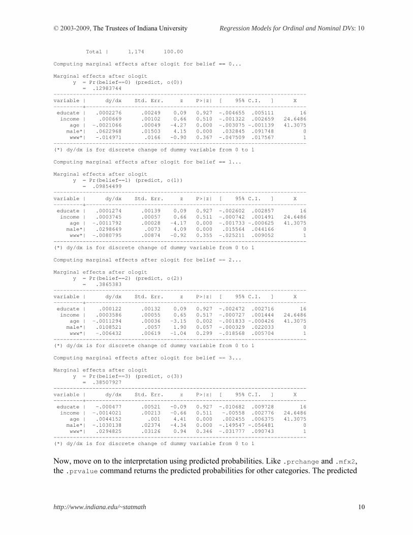
Total | 1,174 100.00 Computing marginal effects after ologit for belief == 0... Marginal effects after ologit y = Pr(belief==0) (predict, o(0)) = .12983744 ------------------------------------------------------------------------------ variable | dy/dx Std. Err. z P>|z| [ 95% C.I. ] X ---------+-------------------------------------------------------------------- educate | .0002276 .00249 0.09 0.927 -.004655 .005111 16 income | .000669 .00102 0.66 0.510 -.001322 .002659 24.6486 age | -.0021066 .00049 -4.27 0.000 -.003075 -.001139 41.3075 male*| .0622968 .01503 4.15 0.000 .032845 .091748 0 www*| -.014971 .0166 -0.90 0.367 -.047509 .017567 1 ------------------------------------------------------------------------------ (*) dy/dx is for discrete change of dummy variable from 0 to 1 Computing marginal effects after ologit for belief == 1... Marginal effects after ologit y = Pr(belief==1) (predict, o(1)) = .09854499 ------------------------------------------------------------------------------ variable | dy/dx Std. Err. z P>|z| [ 95% C.I. ] X ---------+-------------------------------------------------------------------- educate | .0001274 .00139 0.09 0.927 -.002602 .002857 16 income | .0003745 .00057 0.66 0.511 -.000742 .001491 24.6486 age | -.0011792 .00028 -4.17 0.000 -.001733 -.000625 41.3075 male*| .0298649 .0073 4.09 0.000 .015564 .044166 0 www*| -.0080795 .00874 -0.92 0.355 -.025211 .009052 1 ------------------------------------------------------------------------------ (*) dy/dx is for discrete change of dummy variable from 0 to 1 Computing marginal effects after ologit for belief == 2... Marginal effects after ologit y = Pr(belief==2) (predict, o(2)) = .3865383 ------------------------------------------------------------------------------ variable | dy/dx Std. Err. z P>|z| [ 95% C.I. ] X ---------+-------------------------------------------------------------------- educate | .000122 .00132 0.09 0.927 -.002472 .002716 16 income | .0003586 .00055 0.65 0.517 -.000727 .001444 24.6486 age | -.0011294 .00036 -3.15 0.002 -.001833 -.000426 41.3075 male*| .0108521 .0057 1.90 0.057 -.000329 .022033 0 www*| -.006432 .00619 -1.04 0.299 -.018568 .005704 1 ------------------------------------------------------------------------------ (*) dy/dx is for discrete change of dummy variable from 0 to 1 Computing marginal effects after ologit for belief == 3... Marginal effects after ologit y = Pr(belief==3) (predict, o(3)) = .38507927 ------------------------------------------------------------------------------ variable | dy/dx Std. Err. z P>|z| [ 95% C.I. ] X ---------+-------------------------------------------------------------------- educate | -.000477 .00521 -0.09 0.927 -.010682 .009728 16 income | -.0014021 .00213 -0.66 0.511 -.00558 .002776 24.6486 age | .0044152 .001 4.41 0.000 .002455 .006375 41.3075 male*| -.1030138 .02374 -4.34 0.000 -.149547 -.056481 0 www*| .0294825 .03126 0.94 0.346 -.031777 .090743 1 ------------------------------------------------------------------------------ (*) dy/dx is for discrete change of dummy variable from 0 to 1
Now, move on to the interpretation using predicted probabilities. Like .prchange and .mfx2, the .prvalue command returns the predicted probabilities for other categories. The predicted
© 2003-2009, The Trustees of Indiana University Regression Models for Ordinal and Nominal DVs: 11
http://www.indiana.edu/~statmath 11
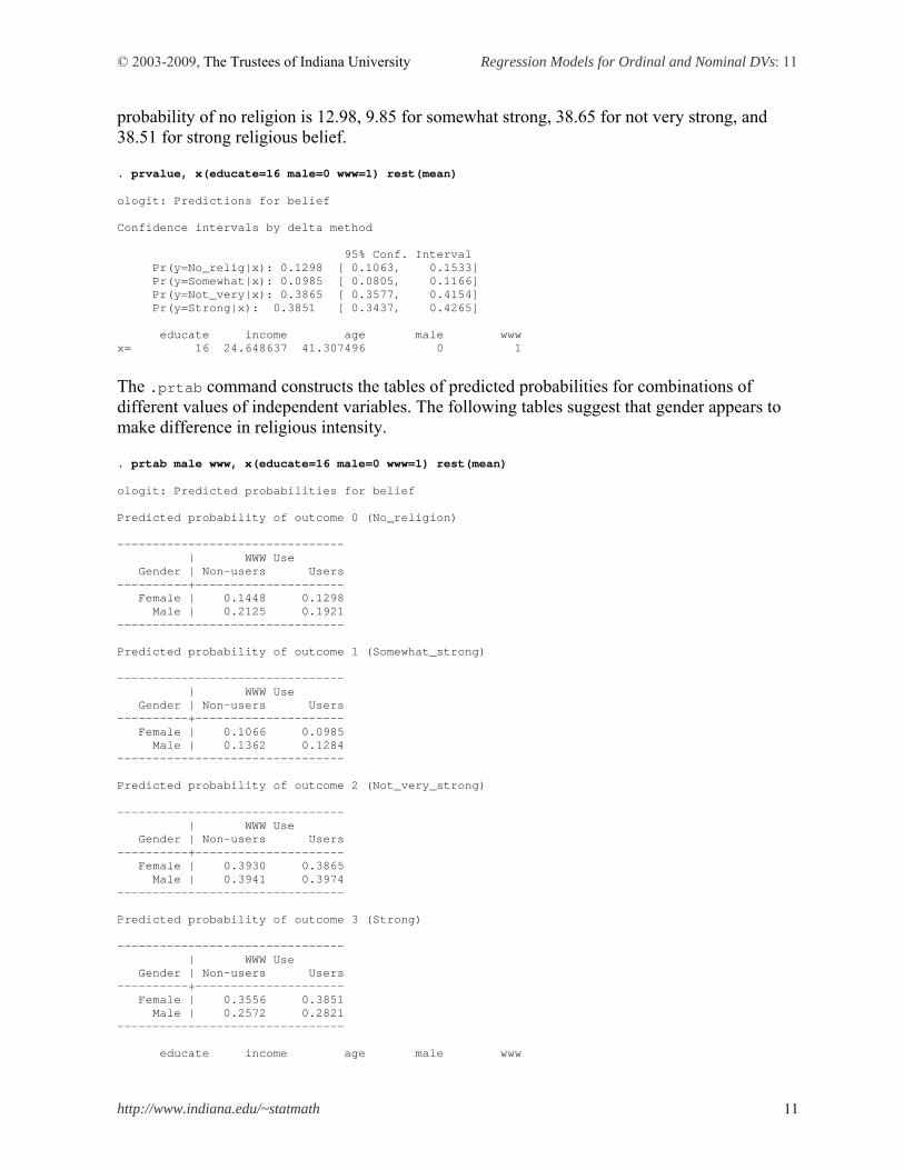
probability of no religion is 12.98, 9.85 for somewhat strong, 38.65 for not very strong, and 38.51 for strong religious belief. . prvalue, x(educate=16 male=0 www=1) rest(mean) ologit: Predictions for belief Confidence intervals by delta method 95% Conf. Interval Pr(y=No_relig|x): 0.1298 [ 0.1063, 0.1533] Pr(y=Somewhat|x): 0.0985 [ 0.0805, 0.1166] Pr(y=Not_very|x): 0.3865 [ 0.3577, 0.4154] Pr(y=Strong|x): 0.3851 [ 0.3437, 0.4265] educate income age male www x= 16 24.648637 41.307496 0 1
The .prtab command constructs the tables of predicted probabilities for combinations of different values of independent variables. The following tables suggest that gender appears to make difference in religious intensity. . prtab male www, x(educate=16 male=0 www=1) rest(mean) ologit: Predicted probabilities for belief Predicted probability of outcome 0 (No_religion) -------------------------------- | WWW Use Gender | Non-users Users ----------+--------------------- Female | 0.1448 0.1298 Male | 0.2125 0.1921 -------------------------------- Predicted probability of outcome 1 (Somewhat_strong) -------------------------------- | WWW Use Gender | Non-users Users ----------+--------------------- Female | 0.1066 0.0985 Male | 0.1362 0.1284 -------------------------------- Predicted probability of outcome 2 (Not_very_strong) -------------------------------- | WWW Use Gender | Non-users Users ----------+--------------------- Female | 0.3930 0.3865 Male | 0.3941 0.3974 -------------------------------- Predicted probability of outcome 3 (Strong) -------------------------------- | WWW Use Gender | Non-users Users ----------+--------------------- Female | 0.3556 0.3851 Male | 0.2572 0.2821 -------------------------------- educate income age male www
© 2003-2009, The Trustees of Indiana University Regression Models for Ordinal and Nominal DVs: 12
http://www.indiana.edu/~statmath 12
x= 16 24.648637 41.307496 0 1
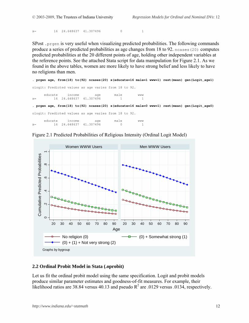
SPost .prgen is very useful when visualizing predicted probabilities. The following commands produce a series of predicted probabilities as age changes from 18 to 92. ncases(20) computes predicted probabilities at the 20 different points of age, holding other independent variables at the reference points. See the attached Stata script for data manipulation for Figure 2.1. As we found in the above tables, women are more likely to have strong belief and less likely to have no religions than men. . prgen age, from(18) to(92) ncases(20) x(educate=16 male=1 www=1) rest(mean) gen(Logit_age1) ologit: Predicted values as age varies from 18 to 92. educate income age male www x= 16 24.648637 41.307496 1 1 . prgen age, from(18) to(92) ncases(20) x(educate=16 male=0 www=1) rest(mean) gen(Logit_age0) ologit: Predicted values as age varies from 18 to 92. educate income age male www x= 16 24.648637 41.307496 0 1
Figure 2.1 Predicted Probabilities of Religious Intensity (Ordinal Logit Model)
0.2
.4.6
.81
20 30 40 50 60 70 80 90 20 30 40 50 60 70 80 90
Women WWW Users Men WWW Users
No religion (0) (0) + Somewhat strong (1)
(0) + (1) + Not very strong (2)
Cum
ula
tive
Pre
dic
ted
Pro
bab
ilitie
s
Age
Graphs by bygroup
2.2 Ordinal Probit Model in Stata (.oprobit)
Let us fit the ordinal probit model using the same specification. Logit and probit models produce similar parameter estimates and goodness-of-fit measures. For example, their likelihood ratios are 38.84 versus 40.13 and pseudo R2 are .0129 versus .0134, respectively.
© 2003-2009, The Trustees of Indiana University Regression Models for Ordinal and Nominal DVs: 13
http://www.indiana.edu/~statmath 13
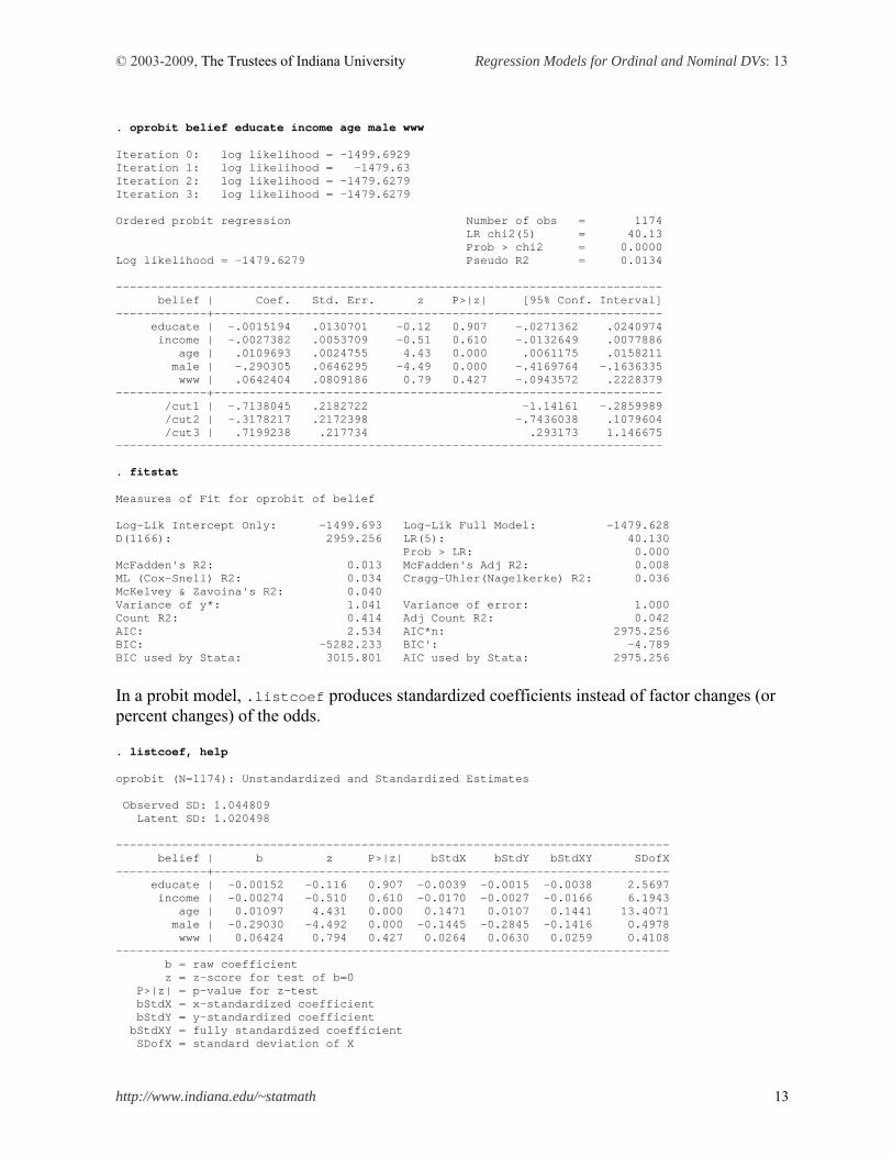
. oprobit belief educate income age male www Iteration 0: log likelihood = -1499.6929 Iteration 1: log likelihood = -1479.63 Iteration 2: log likelihood = -1479.6279 Iteration 3: log likelihood = -1479.6279 Ordered probit regression Number of obs = 1174 LR chi2(5) = 40.13 Prob > chi2 = 0.0000 Log likelihood = -1479.6279 Pseudo R2 = 0.0134 ------------------------------------------------------------------------------ belief | Coef. Std. Err. z P>|z| [95% Conf. Interval] -------------+---------------------------------------------------------------- educate | -.0015194 .0130701 -0.12 0.907 -.0271362 .0240974 income | -.0027382 .0053709 -0.51 0.610 -.0132649 .0077886 age | .0109693 .0024755 4.43 0.000 .0061175 .0158211 male | -.290305 .0646295 -4.49 0.000 -.4169764 -.1636335 www | .0642404 .0809186 0.79 0.427 -.0943572 .2228379 -------------+---------------------------------------------------------------- /cut1 | -.7138045 .2182722 -1.14161 -.2859989 /cut2 | -.3178217 .2172398 -.7436038 .1079604 /cut3 | .7199238 .217734 .293173 1.146675 ------------------------------------------------------------------------------ . fitstat Measures of Fit for oprobit of belief Log-Lik Intercept Only: -1499.693 Log-Lik Full Model: -1479.628 D(1166): 2959.256 LR(5): 40.130 Prob > LR: 0.000 McFadden's R2: 0.013 McFadden's Adj R2: 0.008 ML (Cox-Snell) R2: 0.034 Cragg-Uhler(Nagelkerke) R2: 0.036 McKelvey & Zavoina's R2: 0.040 Variance of y*: 1.041 Variance of error: 1.000 Count R2: 0.414 Adj Count R2: 0.042 AIC: 2.534 AIC*n: 2975.256 BIC: -5282.233 BIC': -4.789 BIC used by Stata: 3015.801 AIC used by Stata: 2975.256
In a probit model, .listcoef produces standardized coefficients instead of factor changes (or percent changes) of the odds. . listcoef, help oprobit (N=1174): Unstandardized and Standardized Estimates Observed SD: 1.044809 Latent SD: 1.020498 ------------------------------------------------------------------------------- belief | b z P>|z| bStdX bStdY bStdXY SDofX -------------+----------------------------------------------------------------- educate | -0.00152 -0.116 0.907 -0.0039 -0.0015 -0.0038 2.5697 income | -0.00274 -0.510 0.610 -0.0170 -0.0027 -0.0166 6.1943 age | 0.01097 4.431 0.000 0.1471 0.0107 0.1441 13.4071 male | -0.29030 -4.492 0.000 -0.1445 -0.2845 -0.1416 0.4978 www | 0.06424 0.794 0.427 0.0264 0.0630 0.0259 0.4108 ------------------------------------------------------------------------------- b = raw coefficient z = z-score for test of b=0 P>|z| = p-value for z-test bStdX = x-standardized coefficient bStdY = y-standardized coefficient bStdXY = fully standardized coefficient SDofX = standard deviation of X
© 2003-2009, The Trustees of Indiana University Regression Models for Ordinal and Nominal DVs: 14
http://www.indiana.edu/~statmath 14
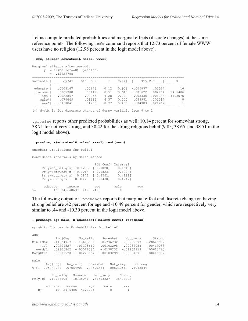
Let us compute predicted probabilities and marginal effects (discrete changes) at the same reference points. The following .mfx command reports that 12.73 percent of female WWW users have no religion (12.98 percent in the logit model above). . mfx, at(mean educate=16 male=0 www=1) Marginal effects after oprobit y = Pr(belief==0) (predict) = .12727708 ------------------------------------------------------------------------------ variable | dy/dx Std. Err. z P>|z| [ 95% C.I. ] X ---------+-------------------------------------------------------------------- educate | .0003167 .00273 0.12 0.908 -.005037 .00567 16 income | .0005708 .00112 0.51 0.610 -.001622 .002764 24.6486 age | -.0022867 .00053 -4.28 0.000 -.003335 -.001238 41.3075 male*| .070649 .01616 4.37 0.000 .038981 .102317 0 www*| -.0138841 .01793 -0.77 0.439 -.04903 .021262 1 ------------------------------------------------------------------------------ (*) dy/dx is for discrete change of dummy variable from 0 to 1
.prvalue reports other predicted probabilities as well: 10.14 percent for somewhat strong, 38.71 for not very strong, and 38.42 for the strong religious belief (9.85, 38.65, and 38.51 in the logit model above). . prvalue, x(educate=16 male=0 www=1) rest(mean) oprobit: Predictions for belief Confidence intervals by delta method 95% Conf. Interval Pr(y=No_relig|x): 0.1273 [ 0.1028, 0.1518] Pr(y=Somewhat|x): 0.1014 [ 0.0823, 0.1204] Pr(y=Not_very|x): 0.3871 [ 0.3561, 0.4182] Pr(y=Strong|x): 0.3842 [ 0.3438, 0.4247] educate income age male www x= 16 24.648637 41.307496 0 1
The following output of .prchange reports that marginal effect and discrete change on having strong belief are .42 percent for age and -10.49 percent for gender, which are respectively very similar to .44 and -10.30 percent in the logit model above. . prchange age male, x(educate=16 male=0 www=1) rest(mean) oprobit: Changes in Probabilities for belief age Avg|Chg| No_relig Somewhat Not_very Strong Min->Max .14324967 -.13683906 -.06736732 -.08229297 .28649932 -+1/2 .00209527 -.00228667 -.00103298 -.00087088 .00419053 -+sd/2 .02806862 -.03066584 -.0138232 -.01164818 .05613723 MargEfct .00209528 -.00228667 -.00103299 -.00087091 .00419057 male Avg|Chg| No_relig Somewhat Not_very Strong 0->1 .05242721 .07064901 .02597284 .00823256 -.1048544 No_relig Somewhat Not_very Strong Pr(y|x) .12727708 .10135041 .38713527 .38423723 educate income age male www x= 16 24.6486 41.3075 0 1
© 2003-2009, The Trustees of Indiana University Regression Models for Ordinal and Nominal DVs: 15
http://www.indiana.edu/~statmath 15
sd_x= 2.56971 6.19427 13.4071 .497765 .410755
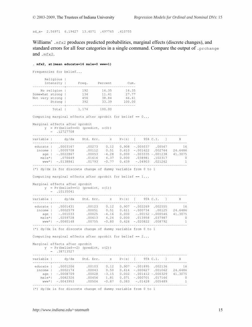
Williams’ .mfx2 produces predicted probabilities, marginal effects (discrete changes), and standard errors for all four categories in a single command. Compare the output of .prchange and .mfx2. . mfx2, at(mean educate=16 male=0 www=1) Frequencies for belief... Religious | Intensity | Freq. Percent Cum. ----------------+----------------------------------- No religion | 192 16.35 16.35 Somewhat strong | 134 11.41 27.77 Not very strong | 456 38.84 66.61 Strong | 392 33.39 100.00 ----------------+----------------------------------- Total | 1,174 100.00 Computing marginal effects after oprobit for belief == 0... Marginal effects after oprobit y = Pr(belief==0) (predict, o(0)) = .12727708 ------------------------------------------------------------------------------ variable | dy/dx Std. Err. z P>|z| [ 95% C.I. ] X ---------+-------------------------------------------------------------------- educate | .0003167 .00273 0.12 0.908 -.005037 .00567 16 income | .0005708 .00112 0.51 0.610 -.001622 .002764 24.6486 age | -.0022867 .00053 -4.28 0.000 -.003335 -.001238 41.3075 male*| .070649 .01616 4.37 0.000 .038981 .102317 0 www*| -.0138841 .01793 -0.77 0.439 -.04903 .021262 1 ------------------------------------------------------------------------------ (*) dy/dx is for discrete change of dummy variable from 0 to 1 Computing marginal effects after oprobit for belief == 1... Marginal effects after oprobit y = Pr(belief==1) (predict, o(1)) = .10135041 ------------------------------------------------------------------------------ variable | dy/dx Std. Err. z P>|z| [ 95% C.I. ] X ---------+-------------------------------------------------------------------- educate | .0001431 .00123 0.12 0.907 -.002269 .002555 16 income | .0002579 .00051 0.51 0.611 -.000734 .00125 24.6486 age | -.001033 .00025 -4.16 0.000 -.00152 -.000546 41.3075 male*| .0259728 .00613 4.24 0.000 .013958 .037987 0 www*| -.0060148 .00755 -0.80 0.426 -.020822 .008792 1 ------------------------------------------------------------------------------ (*) dy/dx is for discrete change of dummy variable from 0 to 1 Computing marginal effects after oprobit for belief == 2... Marginal effects after oprobit y = Pr(belief==2) (predict, o(2)) = .38713527 ------------------------------------------------------------------------------ variable | dy/dx Std. Err. z P>|z| [ 95% C.I. ] X ---------+-------------------------------------------------------------------- educate | .0001206 .00103 0.12 0.907 -.001895 .002136 16 income | .0002174 .00043 0.50 0.614 -.000627 .001062 24.6486 age | -.0008709 .00028 -3.15 0.002 -.001412 -.000329 41.3075 male*| .0082326 .00456 1.81 0.071 -.000701 .017166 0 www*| -.0043953 .00504 -0.87 0.383 -.01428 .005489 1 ------------------------------------------------------------------------------ (*) dy/dx is for discrete change of dummy variable from 0 to 1
© 2003-2009, The Trustees of Indiana University Regression Models for Ordinal and Nominal DVs: 16
http://www.indiana.edu/~statmath 16
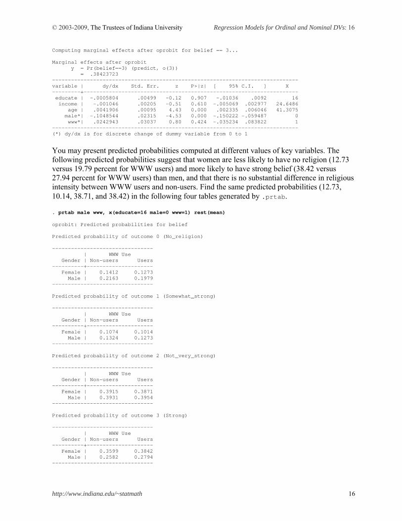
Computing marginal effects after oprobit for belief == 3... Marginal effects after oprobit y = Pr(belief==3) (predict, o(3)) = .38423723 ------------------------------------------------------------------------------ variable | dy/dx Std. Err. z P>|z| [ 95% C.I. ] X ---------+-------------------------------------------------------------------- educate | -.0005804 .00499 -0.12 0.907 -.01036 .0092 16 income | -.001046 .00205 -0.51 0.610 -.005069 .002977 24.6486 age | .0041906 .00095 4.43 0.000 .002335 .006046 41.3075 male*| -.1048544 .02315 -4.53 0.000 -.150222 -.059487 0 www*| .0242943 .03037 0.80 0.424 -.035234 .083822 1 ------------------------------------------------------------------------------ (*) dy/dx is for discrete change of dummy variable from 0 to 1
You may present predicted probabilities computed at different values of key variables. The following predicted probabilities suggest that women are less likely to have no religion (12.73 versus 19.79 percent for WWW users) and more likely to have strong belief (38.42 versus 27.94 percent for WWW users) than men, and that there is no substantial difference in religious intensity between WWW users and non-users. Find the same predicted probabilities (12.73, 10.14, 38.71, and 38.42) in the following four tables generated by .prtab. . prtab male www, x(educate=16 male=0 www=1) rest(mean) oprobit: Predicted probabilities for belief Predicted probability of outcome 0 (No_religion) -------------------------------- | WWW Use Gender | Non-users Users ----------+--------------------- Female | 0.1412 0.1273 Male | 0.2163 0.1979 -------------------------------- Predicted probability of outcome 1 (Somewhat_strong) -------------------------------- | WWW Use Gender | Non-users Users ----------+--------------------- Female | 0.1074 0.1014 Male | 0.1324 0.1273 -------------------------------- Predicted probability of outcome 2 (Not_very_strong) -------------------------------- | WWW Use Gender | Non-users Users ----------+--------------------- Female | 0.3915 0.3871 Male | 0.3931 0.3954 -------------------------------- Predicted probability of outcome 3 (Strong) -------------------------------- | WWW Use Gender | Non-users Users ----------+--------------------- Female | 0.3599 0.3842 Male | 0.2582 0.2794 --------------------------------
© 2003-2009, The Trustees of Indiana University Regression Models for Ordinal and Nominal DVs: 17
http://www.indiana.edu/~statmath 17
educate income age male www x= 16 24.648637 41.307496 0 1
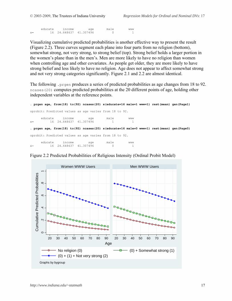
Visualizing cumulative predicted probabilities is another effective way to present the result (Figure 2.2). Three curves segment each plane into four parts from no religion (bottom), somewhat strong, not very strong, to strong belief (top). Strong belief holds a larger portion in the women’s plane than in the men’s. Men are more likely to have no religion than women when controlling age and other covariates. As people get older, they are more likely to have strong belief and less likely to have no religion. Age does not appear to affect somewhat strong and not very strong categories significantly. Figure 2.1 and 2.2 are almost identical. The following .prgen produces a series of predicted probabilities as age changes from 18 to 92. ncases(20) computes predicted probabilities at the 20 different points of age, holding other independent variables at the reference points. . prgen age, from(18) to(92) ncases(20) x(educate=16 male=1 www=1) rest(mean) gen(Page1) oprobit: Predicted values as age varies from 18 to 92. educate income age male www x= 16 24.648637 41.307496 1 1 . prgen age, from(18) to(92) ncases(20) x(educate=16 male=0 www=1) rest(mean) gen(Page0) oprobit: Predicted values as age varies from 18 to 92. educate income age male www x= 16 24.648637 41.307496 0 1 Figure 2.2 Predicted Probabilities of Religious Intensity (Ordinal Probit Model)
0.2
.4.6
.81
20 30 40 50 60 70 80 90 20 30 40 50 60 70 80 90
Women WWW Users Men WWW Users
No religion (0) (0) + Somewhat strong (1)
(0) + (1) + Not very strong (2)
Cum
ula
tive
Pre
dic
ted
Pro
bab
ilitie
s
Age
Graphs by bygroup
© 2003-2009, The Trustees of Indiana University Regression Models for Ordinal and Nominal DVs: 18
http://www.indiana.edu/~statmath 18
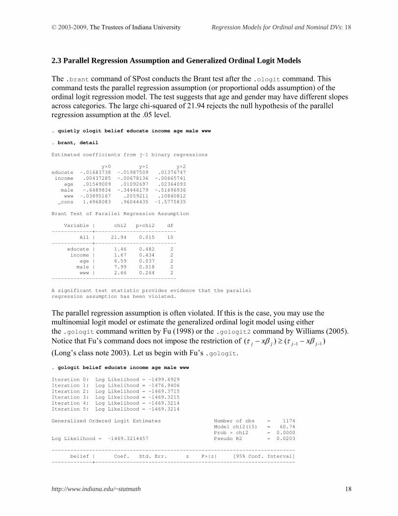
2.3 Parallel Regression Assumption and Generalized Ordinal Logit Models The .brant command of SPost conducts the Brant test after the .ologit command. This command tests the parallel regression assumption (or proportional odds assumption) of the ordinal logit regression model. The test suggests that age and gender may have different slopes across categories. The large chi-squared of 21.94 rejects the null hypothesis of the parallel regression assumption at the .05 level. . quietly ologit belief educate income age male www . brant, detail Estimated coefficients from j-1 binary regressions y>0 y>1 y>2 educate -.01683738 -.01987509 .01376747 income .00437285 -.00678136 -.00665741 age .01549009 .01092697 .02364093 male -.6489834 -.34446179 -.51696936 www -.03895167 .2059211 .10840812 _cons 1.4968083 .96044435 -1.5775835 Brant Test of Parallel Regression Assumption Variable | chi2 p>chi2 df -------------+-------------------------- All | 21.94 0.015 10 -------------+-------------------------- educate | 1.46 0.482 2 income | 1.67 0.434 2 age | 6.59 0.037 2 male | 7.99 0.018 2 www | 2.66 0.264 2 ---------------------------------------- A significant test statistic provides evidence that the parallel regression assumption has been violated.
The parallel regression assumption is often violated. If this is the case, you may use the multinomial logit model or estimate the generalized ordinal logit model using either the .gologit command written by Fu (1998) or the .gologit2 command by Williams (2005). Notice that Fu’s command does not impose the restriction of )()( 11 jjjj xx
(Long’s class note 2003). Let us begin with Fu’s .gologit. . gologit belief educate income age male www Iteration 0: Log Likelihood = -1499.6929 Iteration 1: Log Likelihood = -1476.9406 Iteration 2: Log Likelihood = -1469.3715 Iteration 3: Log Likelihood = -1469.3215 Iteration 4: Log Likelihood = -1469.3214 Iteration 5: Log Likelihood = -1469.3214 Generalized Ordered Logit Estimates Number of obs = 1174 Model chi2(15) = 60.74 Prob > chi2 = 0.0000 Log Likelihood = -1469.3214457 Pseudo R2 = 0.0203 ------------------------------------------------------------------------------ belief | Coef. Std. Err. z P>|z| [95% Conf. Interval] -------------+----------------------------------------------------------------
© 2003-2009, The Trustees of Indiana University Regression Models for Ordinal and Nominal DVs: 19
http://www.indiana.edu/~statmath 19
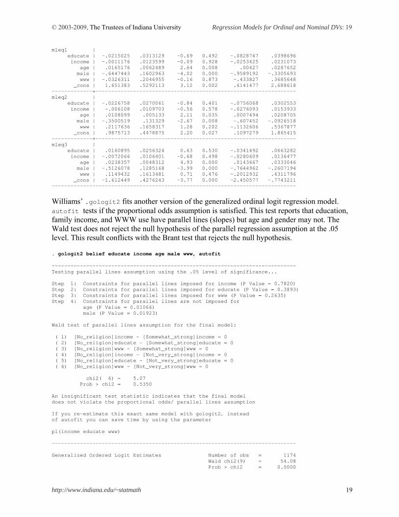
mleq1 | educate | -.0215025 .0313129 -0.69 0.492 -.0828747 .0398696 income | -.0011176 .0123599 -0.09 0.928 -.0253425 .0231073 age | .0165176 .0062489 2.64 0.008 .00427 .0287652 male | -.6447443 .1602963 -4.02 0.000 -.9589192 -.3305693 www | -.0326311 .2046955 -0.16 0.873 -.433827 .3685648 _cons | 1.651383 .5292113 3.12 0.002 .6141477 2.688618 -------------+---------------------------------------------------------------- mleq2 | educate | -.0226758 .0270061 -0.84 0.401 -.0756068 .0302553 income | -.006108 .0109703 -0.56 0.578 -.0276093 .0153933 age | .0108099 .005133 2.11 0.035 .0007494 .0208705 male | -.3500519 .131329 -2.67 0.008 -.607452 -.0926518 www | .2117636 .1658317 1.28 0.202 -.1132606 .5367877 _cons | .9875713 .4478875 2.20 0.027 .1097279 1.865415 -------------+---------------------------------------------------------------- mleq3 | educate | .0160895 .0256324 0.63 0.530 -.0341492 .0663282 income | -.0072066 .0106401 -0.68 0.498 -.0280609 .0136477 age | .0238357 .0048312 4.93 0.000 .0143667 .0333046 male | -.5126078 .1285168 -3.99 0.000 -.7644962 -.2607194 www | .1149432 .1613481 0.71 0.476 -.2012932 .4311796 _cons | -1.612449 .4276243 -3.77 0.000 -2.450577 -.7743211 ------------------------------------------------------------------------------
Williams’ .gologit2 fits another version of the generalized ordinal logit regression model. autofit tests if the proportional odds assumption is satisfied. This test reports that education, family income, and WWW use have parallel lines (slopes) but age and gender may not. The Wald test does not reject the null hypothesis of the parallel regression assumption at the .05 level. This result conflicts with the Brant test that rejects the null hypothesis. . gologit2 belief educate income age male www, autofit ------------------------------------------------------------------------------ Testing parallel lines assumption using the .05 level of significance... Step 1: Constraints for parallel lines imposed for income (P Value = 0.7820) Step 2: Constraints for parallel lines imposed for educate (P Value = 0.3893) Step 3: Constraints for parallel lines imposed for www (P Value = 0.2635) Step 4: Constraints for parallel lines are not imposed for age (P Value = 0.01066) male (P Value = 0.01923) Wald test of parallel lines assumption for the final model: ( 1) [No_religion]income - [Somewhat_strong]income = 0 ( 2) [No_religion]educate - [Somewhat_strong]educate = 0 ( 3) [No_religion]www - [Somewhat_strong]www = 0 ( 4) [No_religion]income - [Not_very_strong]income = 0 ( 5) [No_religion]educate - [Not_very_strong]educate = 0 ( 6) [No_religion]www - [Not_very_strong]www = 0 chi2( 6) = 5.07 Prob > chi2 = 0.5350 An insignificant test statistic indicates that the final model does not violate the proportional odds/ parallel lines assumption If you re-estimate this exact same model with gologit2, instead of autofit you can save time by using the parameter pl(income educate www) ------------------------------------------------------------------------------ Generalized Ordered Logit Estimates Number of obs = 1174 Wald chi2(9) = 54.08 Prob > chi2 = 0.0000
© 2003-2009, The Trustees of Indiana University Regression Models for Ordinal and Nominal DVs: 20
http://www.indiana.edu/~statmath 20
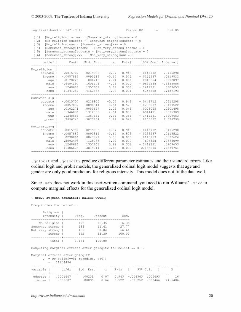
Log likelihood = -1471.9949 Pseudo R2 = 0.0185 ( 1) [No_religion]income - [Somewhat_strong]income = 0 ( 2) [No_religion]educate - [Somewhat_strong]educate = 0 ( 3) [No_religion]www - [Somewhat_strong]www = 0 ( 4) [Somewhat_strong]income - [Not_very_strong]income = 0 ( 5) [Somewhat_strong]educate - [Not_very_strong]educate = 0 ( 6) [Somewhat_strong]www - [Not_very_strong]www = 0 ------------------------------------------------------------------------------ belief | Coef. Std. Err. z P>|z| [95% Conf. Interval] -------------+---------------------------------------------------------------- No_religion | educate | -.0015707 .0219905 -0.07 0.943 -.0446712 .0415298 income | -.0057882 .0090514 -0.64 0.523 -.0235287 .0119522 age | .0170225 .006218 2.74 0.006 .0048354 .0292097 male | -.6494197 .1601173 -4.06 0.000 -.9632438 -.3355956 www | .1248686 .1357661 0.92 0.358 -.1412281 .3909653 _cons | 1.341287 .4162863 3.22 0.001 .5253808 2.157193 -------------+---------------------------------------------------------------- Somewhat_s~g | educate | -.0015707 .0219905 -0.07 0.943 -.0446712 .0415298 income | -.0057882 .0090514 -0.64 0.523 -.0235287 .0119522 age | .0102271 .0050627 2.02 0.043 .0003045 .0201498 male | -.346836 .1312805 -2.64 0.008 -.6041411 -.0895309 www | .1248686 .1357661 0.92 0.358 -.1412281 .3909653 _cons | .7696745 .3873154 1.99 0.047 .0105502 1.528799 -------------+---------------------------------------------------------------- Not_very_s~g | educate | -.0015707 .0219905 -0.07 0.943 -.0446712 .0415298 income | -.0057882 .0090514 -0.64 0.523 -.0235287 .0119522 age | .0238896 .0047821 5.00 0.000 .0145169 .0332624 male | -.5092498 .128288 -3.97 0.000 -.7606898 -.2578099 www | .1248686 .1357661 0.92 0.358 -.1412281 .3909653 _cons | -1.406625 .3819714 -3.68 0.000 -2.155275 -.6579751 ------------------------------------------------------------------------------
.gologit and .gologit2 produce different parameter estimates and their standard errors. Like ordinal logit and probit models, the generalized ordinal logit model suggests that age and gender are only good predictors for religious intensity. This model does not fit the data well. Since .mfx does not work in this user-written command, you need to run Williams’ .mfx2 to compute marginal effects for the generalized ordinal logit model. . mfx2, at(mean educate=16 male=0 www=1) Frequencies for belief... Religious | Intensity | Freq. Percent Cum. ----------------+----------------------------------- No religion | 192 16.35 16.35 Somewhat strong | 134 11.41 27.77 Not very strong | 456 38.84 66.61 Strong | 392 33.39 100.00 ----------------+----------------------------------- Total | 1,174 100.00 Computing marginal effects after gologit2 for belief == 0... Marginal effects after gologit2 y = Pr(belief==0) (predict, o(0)) = .11904434 ------------------------------------------------------------------------------ variable | dy/dx Std. Err. z P>|z| [ 95% C.I. ] X ---------+-------------------------------------------------------------------- educate | .0001647 .00231 0.07 0.943 -.004363 .004693 16 income | .000607 .00095 0.64 0.522 -.001252 .002466 24.6486
© 2003-2009, The Trustees of Indiana University Regression Models for Ordinal and Nominal DVs: 21
http://www.indiana.edu/~statmath 21
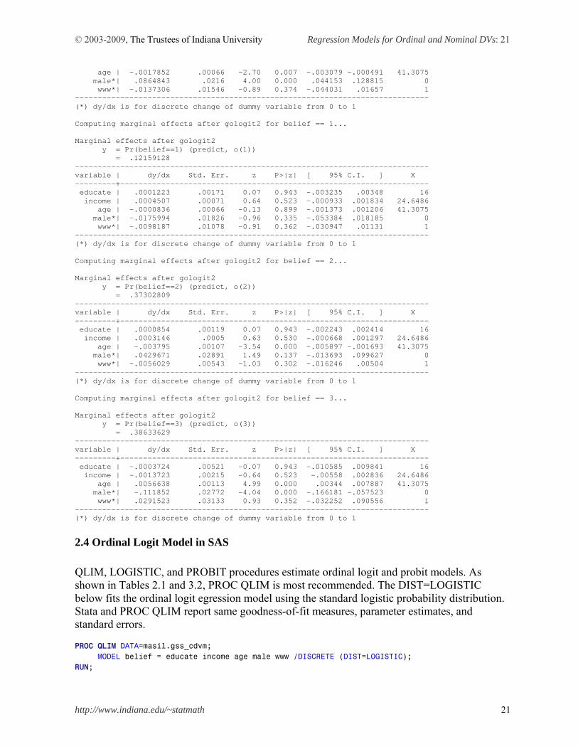
age | -.0017852 .00066 -2.70 0.007 -.003079 -.000491 41.3075 male*| .0864843 .0216 4.00 0.000 .044153 .128815 0 www*| -.0137306 .01546 -0.89 0.374 -.044031 .01657 1 ------------------------------------------------------------------------------ (*) dy/dx is for discrete change of dummy variable from 0 to 1 Computing marginal effects after gologit2 for belief == 1... Marginal effects after gologit2 y = Pr(belief==1) (predict, o(1)) = .12159128 ------------------------------------------------------------------------------ variable | dy/dx Std. Err. z P>|z| [ 95% C.I. ] X ---------+-------------------------------------------------------------------- educate | .0001223 .00171 0.07 0.943 -.003235 .00348 16 income | .0004507 .00071 0.64 0.523 -.000933 .001834 24.6486 age | -.0000836 .00066 -0.13 0.899 -.001373 .001206 41.3075 male*| -.0175994 .01826 -0.96 0.335 -.053384 .018185 0 www*| -.0098187 .01078 -0.91 0.362 -.030947 .01131 1 ------------------------------------------------------------------------------ (*) dy/dx is for discrete change of dummy variable from 0 to 1 Computing marginal effects after gologit2 for belief == 2... Marginal effects after gologit2 y = Pr(belief==2) (predict, o(2)) = .37302809 ------------------------------------------------------------------------------ variable | dy/dx Std. Err. z P>|z| [ 95% C.I. ] X ---------+-------------------------------------------------------------------- educate | .0000854 .00119 0.07 0.943 -.002243 .002414 16 income | .0003146 .0005 0.63 0.530 -.000668 .001297 24.6486 age | -.003795 .00107 -3.54 0.000 -.005897 -.001693 41.3075 male*| .0429671 .02891 1.49 0.137 -.013693 .099627 0 www*| -.0056029 .00543 -1.03 0.302 -.016246 .00504 1 ------------------------------------------------------------------------------ (*) dy/dx is for discrete change of dummy variable from 0 to 1 Computing marginal effects after gologit2 for belief == 3... Marginal effects after gologit2 y = Pr(belief==3) (predict, o(3)) = .38633629 ------------------------------------------------------------------------------ variable | dy/dx Std. Err. z P>|z| [ 95% C.I. ] X ---------+-------------------------------------------------------------------- educate | -.0003724 .00521 -0.07 0.943 -.010585 .009841 16 income | -.0013723 .00215 -0.64 0.523 -.00558 .002836 24.6486 age | .0056638 .00113 4.99 0.000 .00344 .007887 41.3075 male*| -.111852 .02772 -4.04 0.000 -.166181 -.057523 0 www*| .0291523 .03133 0.93 0.352 -.032252 .090556 1 ------------------------------------------------------------------------------ (*) dy/dx is for discrete change of dummy variable from 0 to 1
2.4 Ordinal Logit Model in SAS
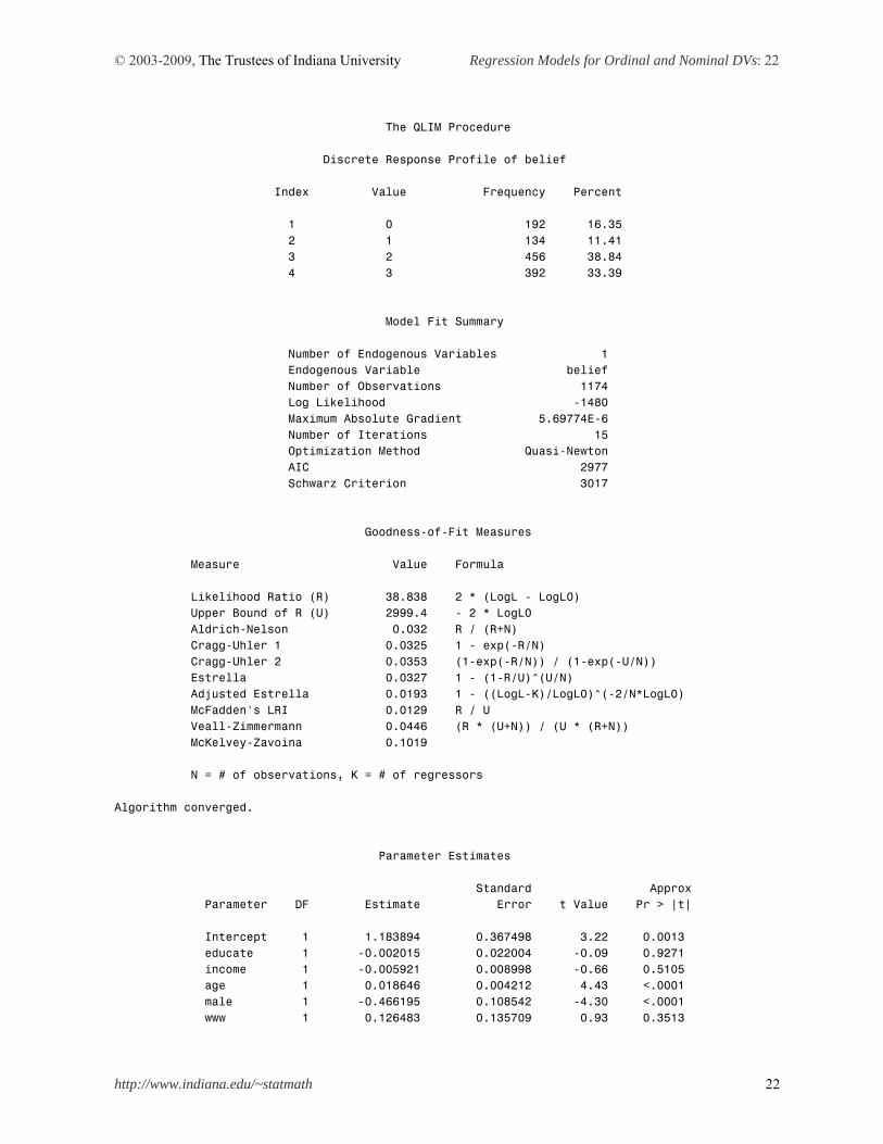
QLIM, LOGISTIC, and PROBIT procedures estimate ordinal logit and probit models. As shown in Tables 2.1 and 3.2, PROC QLIM is most recommended. The DIST=LOGISTIC below fits the ordinal logit egression model using the standard logistic probability distribution. Stata and PROC QLIM report same goodness-of-fit measures, parameter estimates, and standard errors. PROC QLIM DATA=masil.gss_cdvm; MODEL belief = educate income age male www /DISCRETE (DIST=LOGISTIC); RUN;
© 2003-2009, The Trustees of Indiana University Regression Models for Ordinal and Nominal DVs: 22
http://www.indiana.edu/~statmath 22
The QLIM Procedure Discrete Response Profile of belief Index Value Frequency Percent 1 0 192 16.35 2 1 134 11.41 3 2 456 38.84 4 3 392 33.39 Model Fit Summary Number of Endogenous Variables 1 Endogenous Variable belief Number of Observations 1174 Log Likelihood -1480 Maximum Absolute Gradient 5.69774E-6 Number of Iterations 15 Optimization Method Quasi-Newton AIC 2977 Schwarz Criterion 3017 Goodness-of-Fit Measures Measure Value Formula Likelihood Ratio (R) 38.838 2 * (LogL - LogL0) Upper Bound of R (U) 2999.4 - 2 * LogL0 Aldrich-Nelson 0.032 R / (R+N) Cragg-Uhler 1 0.0325 1 - exp(-R/N) Cragg-Uhler 2 0.0353 (1-exp(-R/N)) / (1-exp(-U/N)) Estrella 0.0327 1 - (1-R/U)^(U/N) Adjusted Estrella 0.0193 1 - ((LogL-K)/LogL0)^(-2/N*LogL0) McFadden's LRI 0.0129 R / U Veall-Zimmermann 0.0446 (R * (U+N)) / (U * (R+N)) McKelvey-Zavoina 0.1019 N = # of observations, K = # of regressors Algorithm converged. Parameter Estimates Standard Approx Parameter DF Estimate Error t Value Pr > |t| Intercept 1 1.183894 0.367498 3.22 0.0013 educate 1 -0.002015 0.022004 -0.09 0.9271 income 1 -0.005921 0.008998 -0.66 0.5105 age 1 0.018646 0.004212 4.43 <.0001 male 1 -0.466195 0.108542 -4.30 <.0001 www 1 0.126483 0.135709 0.93 0.3513
© 2003-2009, The Trustees of Indiana University Regression Models for Ordinal and Nominal DVs: 23
http://www.indiana.edu/~statmath 23
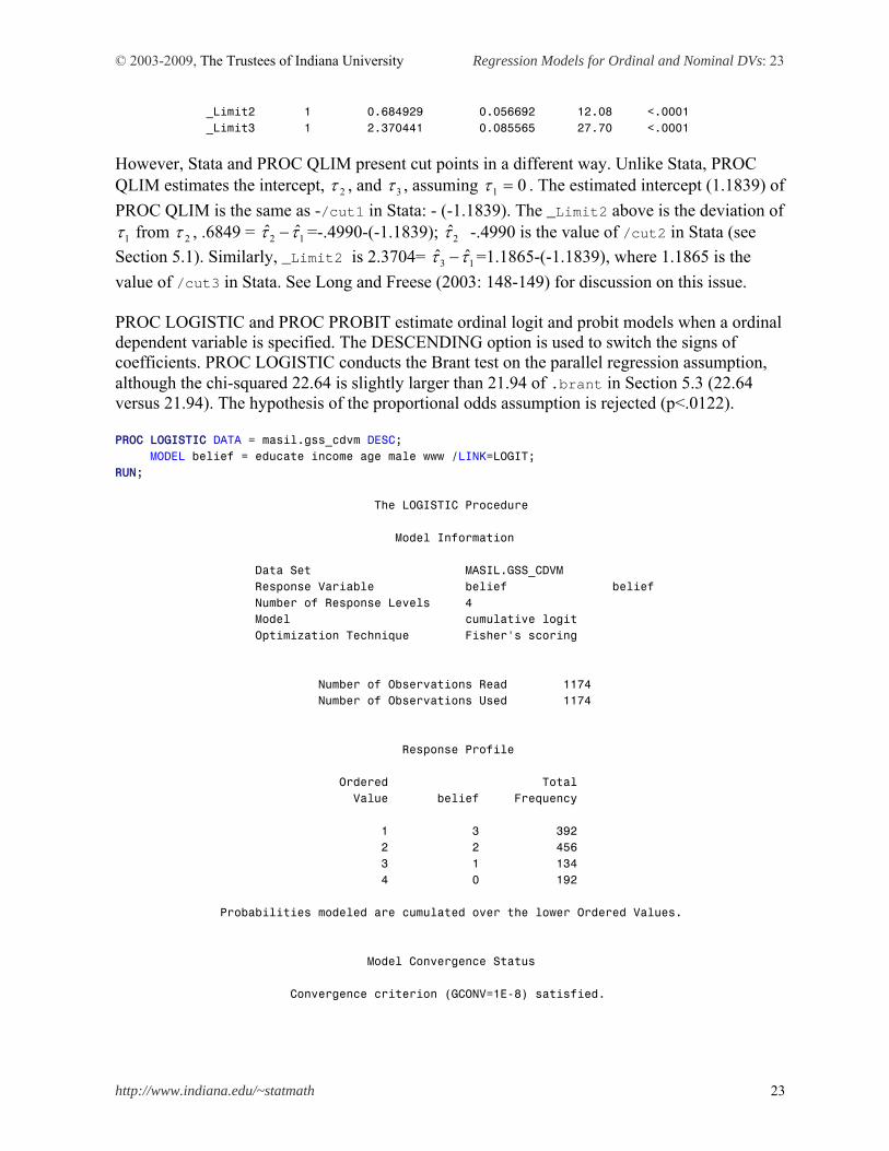
_Limit2 1 0.684929 0.056692 12.08 <.0001 _Limit3 1 2.370441 0.085565 27.70 <.0001
However, Stata and PROC QLIM present cut points in a different way. Unlike Stata, PROC QLIM estimates the intercept, 2 , and 3 , assuming 01 . The estimated intercept (1.1839) of
PROC QLIM is the same as -/cut1 in Stata: - (-1.1839). The _Limit2 above is the deviation of
1 from 2 , .6849 = 12 ˆˆ =-.4990-(-1.1839); 2̂ -.4990 is the value of /cut2 in Stata (see
Section 5.1). Similarly, _Limit2 is 2.3704= 13 ˆˆ =1.1865-(-1.1839), where 1.1865 is the
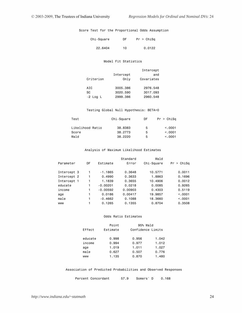
value of /cut3 in Stata. See Long and Freese (2003: 148-149) for discussion on this issue. PROC LOGISTIC and PROC PROBIT estimate ordinal logit and probit models when a ordinal dependent variable is specified. The DESCENDING option is used to switch the signs of coefficients. PROC LOGISTIC conducts the Brant test on the parallel regression assumption, although the chi-squared 22.64 is slightly larger than 21.94 of .brant in Section 5.3 (22.64 versus 21.94). The hypothesis of the proportional odds assumption is rejected (p<.0122). PROC LOGISTIC DATA = masil.gss_cdvm DESC; MODEL belief = educate income age male www /LINK=LOGIT; RUN; The LOGISTIC Procedure Model Information Data Set MASIL.GSS_CDVM Response Variable belief belief Number of Response Levels 4 Model cumulative logit Optimization Technique Fisher's scoring Number of Observations Read 1174 Number of Observations Used 1174 Response Profile Ordered Total Value belief Frequency 1 3 392 2 2 456 3 1 134 4 0 192 Probabilities modeled are cumulated over the lower Ordered Values. Model Convergence Status Convergence criterion (GCONV=1E-8) satisfied.
© 2003-2009, The Trustees of Indiana University Regression Models for Ordinal and Nominal DVs: 24
http://www.indiana.edu/~statmath 24
Score Test for the Proportional Odds Assumption Chi-Square DF Pr > ChiSq 22.6404 10 0.0122 Model Fit Statistics Intercept Intercept and Criterion Only Covariates AIC 3005.386 2976.548 SC 3020.590 3017.093 -2 Log L 2999.386 2960.548 Testing Global Null Hypothesis: BETA=0 Test Chi-Square DF Pr > ChiSq Likelihood Ratio 38.8383 5 <.0001 Score 38.2773 5 <.0001 Wald 38.2220 5 <.0001 Analysis of Maximum Likelihood Estimates Standard Wald Parameter DF Estimate Error Chi-Square Pr > ChiSq Intercept 3 1 -1.1865 0.3648 10.5771 0.0011 Intercept 2 1 0.4990 0.3633 1.8863 0.1696 Intercept 1 1 1.1839 0.3655 10.4906 0.0012 educate 1 -0.00201 0.0218 0.0085 0.9265 income 1 -0.00592 0.00903 0.4303 0.5119 age 1 0.0186 0.00417 19.9857 <.0001 male 1 -0.4662 0.1088 18.3660 <.0001 www 1 0.1265 0.1355 0.8704 0.3508 Odds Ratio Estimates Point 95% Wald Effect Estimate Confidence Limits educate 0.998 0.956 1.042 income 0.994 0.977 1.012 age 1.019 1.011 1.027 male 0.627 0.507 0.776 www 1.135 0.870 1.480 Association of Predicted Probabilities and Observed Responses Percent Concordant 57.9 Somers' D 0.168
© 2003-2009, The Trustees of Indiana University Regression Models for Ordinal and Nominal DVs: 25
http://www.indiana.edu/~statmath 25
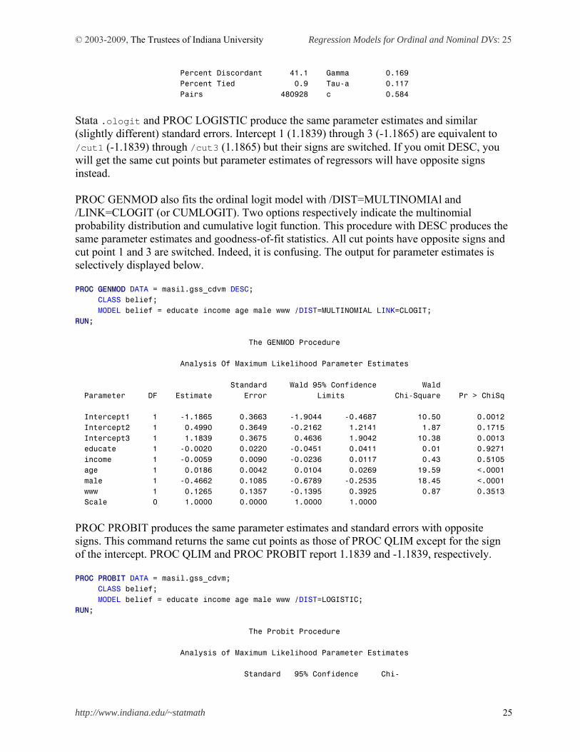
Percent Discordant 41.1 Gamma 0.169 Percent Tied 0.9 Tau-a 0.117 Pairs 480928 c 0.584 Stata .ologit and PROC LOGISTIC produce the same parameter estimates and similar (slightly different) standard errors. Intercept 1 (1.1839) through 3 (-1.1865) are equivalent to /cut1 (-1.1839) through /cut3 (1.1865) but their signs are switched. If you omit DESC, you will get the same cut points but parameter estimates of regressors will have opposite signs instead. PROC GENMOD also fits the ordinal logit model with /DIST=MULTINOMIAl and /LINK=CLOGIT (or CUMLOGIT). Two options respectively indicate the multinomial probability distribution and cumulative logit function. This procedure with DESC produces the same parameter estimates and goodness-of-fit statistics. All cut points have opposite signs and cut point 1 and 3 are switched. Indeed, it is confusing. The output for parameter estimates is selectively displayed below. PROC GENMOD DATA = masil.gss_cdvm DESC; CLASS belief; MODEL belief = educate income age male www /DIST=MULTINOMIAL LINK=CLOGIT; RUN; The GENMOD Procedure Analysis Of Maximum Likelihood Parameter Estimates Standard Wald 95% Confidence Wald Parameter DF Estimate Error Limits Chi-Square Pr > ChiSq Intercept1 1 -1.1865 0.3663 -1.9044 -0.4687 10.50 0.0012 Intercept2 1 0.4990 0.3649 -0.2162 1.2141 1.87 0.1715 Intercept3 1 1.1839 0.3675 0.4636 1.9042 10.38 0.0013 educate 1 -0.0020 0.0220 -0.0451 0.0411 0.01 0.9271 income 1 -0.0059 0.0090 -0.0236 0.0117 0.43 0.5105 age 1 0.0186 0.0042 0.0104 0.0269 19.59 <.0001 male 1 -0.4662 0.1085 -0.6789 -0.2535 18.45 <.0001 www 1 0.1265 0.1357 -0.1395 0.3925 0.87 0.3513
Scale 0 1.0000 0.0000 1.0000 1.0000
PROC PROBIT produces the same parameter estimates and standard errors with opposite signs. This command returns the same cut points as those of PROC QLIM except for the sign of the intercept. PROC QLIM and PROC PROBIT report 1.1839 and -1.1839, respectively. PROC PROBIT DATA = masil.gss_cdvm; CLASS belief; MODEL belief = educate income age male www /DIST=LOGISTIC; RUN; The Probit Procedure Analysis of Maximum Likelihood Parameter Estimates Standard 95% Confidence Chi-
© 2003-2009, The Trustees of Indiana University Regression Models for Ordinal and Nominal DVs: 26
http://www.indiana.edu/~statmath 26
Parameter DF Estimate Error Limits Square Pr > ChiSq Intercept 1 -1.1839 0.3675 -1.9042 -0.4636 10.38 0.0013 Intercept2 1 0.6849 0.0567 0.5738 0.7960 145.97 <.0001 Intercept3 1 2.3704 0.0856 2.2027 2.5381 767.49 <.0001 educate 1 0.0020 0.0220 -0.0411 0.0451 0.01 0.9271 income 1 0.0059 0.0090 -0.0117 0.0236 0.43 0.5105 age 1 -0.0186 0.0042 -0.0269 -0.0104 19.59 <.0001 male 1 0.4662 0.1085 0.2535 0.6789 18.45 <.0001 www 1 -0.1265 0.1357 -0.3925 0.1395 0.87 0.3513
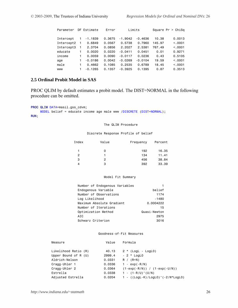
2.5 Ordinal Probit Model in SAS PROC QLIM by default estimates a probit model. The DIST=NORMAL in the following procedure can be omitted. PROC QLIM DATA=masil.gss_cdvm; MODEL belief = educate income age male www /DISCRETE (DIST=NORMAL); RUN; The QLIM Procedure Discrete Response Profile of belief Index Value Frequency Percent 1 0 192 16.35 2 1 134 11.41 3 2 456 38.84 4 3 392 33.39 Model Fit Summary Number of Endogenous Variables 1 Endogenous Variable belief Number of Observations 1174 Log Likelihood -1480 Maximum Absolute Gradient 0.0004222 Number of Iterations 15 Optimization Method Quasi-Newton AIC 2975 Schwarz Criterion 3016 Goodness-of-Fit Measures Measure Value Formula Likelihood Ratio (R) 40.13 2 * (LogL - LogL0) Upper Bound of R (U) 2999.4 - 2 * LogL0 Aldrich-Nelson 0.0331 R / (R+N) Cragg-Uhler 1 0.0336 1 - exp(-R/N) Cragg-Uhler 2 0.0364 (1-exp(-R/N)) / (1-exp(-U/N)) Estrella 0.0338 1 - (1-R/U)^(U/N) Adjusted Estrella 0.0204 1 - ((LogL-K)/LogL0)^(-2/N*LogL0)
© 2003-2009, The Trustees of Indiana University Regression Models for Ordinal and Nominal DVs: 27
http://www.indiana.edu/~statmath 27
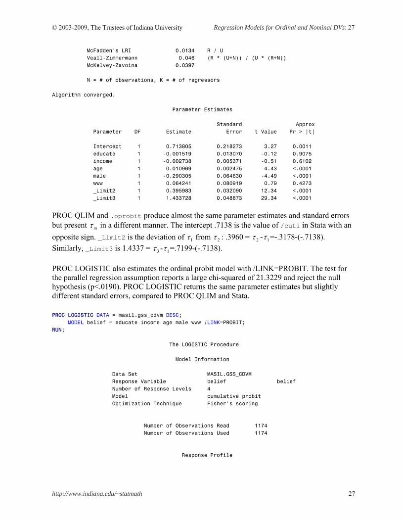
McFadden's LRI 0.0134 R / U Veall-Zimmermann 0.046 (R * (U+N)) / (U * (R+N)) McKelvey-Zavoina 0.0397 N = # of observations, K = # of regressors Algorithm converged. Parameter Estimates Standard Approx Parameter DF Estimate Error t Value Pr > |t| Intercept 1 0.713805 0.218273 3.27 0.0011 educate 1 -0.001519 0.013070 -0.12 0.9075 income 1 -0.002738 0.005371 -0.51 0.6102 age 1 0.010969 0.002475 4.43 <.0001 male 1 -0.290305 0.064630 -4.49 <.0001 www 1 0.064241 0.080919 0.79 0.4273 _Limit2 1 0.395983 0.032090 12.34 <.0001 _Limit3 1 1.433728 0.048873 29.34 <.0001 PROC QLIM and .oprobit produce almost the same parameter estimates and standard errors but present m in a different manner. The intercept .7138 is the value of /cut1 in Stata with an
opposite sign. _Limit2 is the deviation of 1 from 2 : .3960 = 2 - 1 =-.3178-(-.7138).
Similarly, _Limit3 is 1.4337 = 3 - 1 =.7199-(-.7138).
PROC LOGISTIC also estimates the ordinal probit model with /LINK=PROBIT. The test for the parallel regression assumption reports a large chi-squared of 21.3229 and reject the null hypothesis (p<.0190). PROC LOGISTIC returns the same parameter estimates but slightly different standard errors, compared to PROC QLIM and Stata.
PROC LOGISTIC DATA = masil.gss_cdvm DESC; MODEL belief = educate income age male www /LINK=PROBIT; RUN; The LOGISTIC Procedure Model Information Data Set MASIL.GSS_CDVM Response Variable belief belief Number of Response Levels 4 Model cumulative probit Optimization Technique Fisher's scoring Number of Observations Read 1174 Number of Observations Used 1174 Response Profile
© 2003-2009, The Trustees of Indiana University Regression Models for Ordinal and Nominal DVs: 28
http://www.indiana.edu/~statmath 28
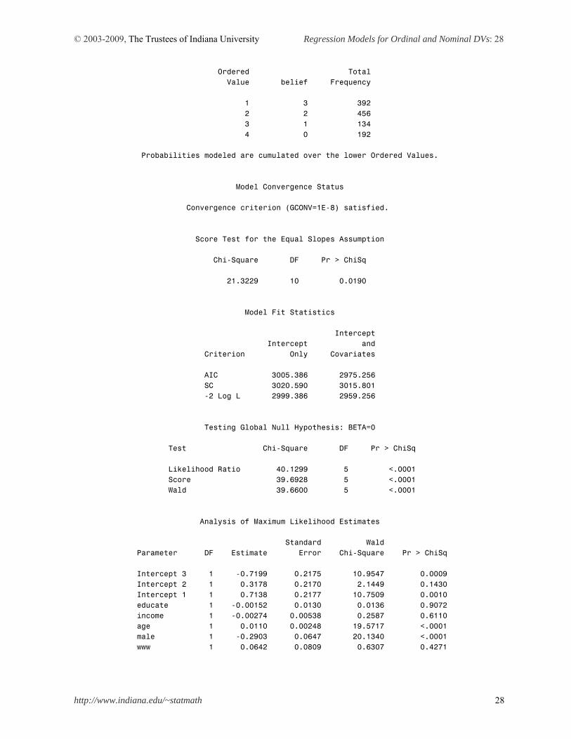
Ordered Total Value belief Frequency 1 3 392 2 2 456 3 1 134 4 0 192 Probabilities modeled are cumulated over the lower Ordered Values. Model Convergence Status Convergence criterion (GCONV=1E-8) satisfied. Score Test for the Equal Slopes Assumption Chi-Square DF Pr > ChiSq 21.3229 10 0.0190 Model Fit Statistics Intercept Intercept and Criterion Only Covariates AIC 3005.386 2975.256 SC 3020.590 3015.801 -2 Log L 2999.386 2959.256 Testing Global Null Hypothesis: BETA=0 Test Chi-Square DF Pr > ChiSq Likelihood Ratio 40.1299 5 <.0001 Score 39.6928 5 <.0001 Wald 39.6600 5 <.0001 Analysis of Maximum Likelihood Estimates Standard Wald Parameter DF Estimate Error Chi-Square Pr > ChiSq Intercept 3 1 -0.7199 0.2175 10.9547 0.0009 Intercept 2 1 0.3178 0.2170 2.1449 0.1430 Intercept 1 1 0.7138 0.2177 10.7509 0.0010 educate 1 -0.00152 0.0130 0.0136 0.9072 income 1 -0.00274 0.00538 0.2587 0.6110 age 1 0.0110 0.00248 19.5717 <.0001 male 1 -0.2903 0.0647 20.1340 <.0001 www 1 0.0642 0.0809 0.6307 0.4271
© 2003-2009, The Trustees of Indiana University Regression Models for Ordinal and Nominal DVs: 29
http://www.indiana.edu/~statmath 29
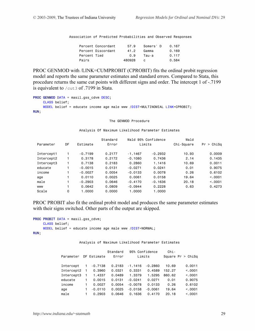
Association of Predicted Probabilities and Observed Responses Percent Concordant 57.9 Somers' D 0.167 Percent Discordant 41.2 Gamma 0.169 Percent Tied 0.9 Tau-a 0.117 Pairs 480928 c 0.584
PROC GENMOD with /LINK=CUMPROBIT (CPROBIT) fits the ordinal probit regression model and reports the same parameter estimates and standard errors. Compared to Stata, this procedure returns the same cut points with different signs and order. The intercept 1 of -.7199 is equivalent to /cut3 of .7199 in Stata. PROC GENMOD DATA = masil.gss_cdvm DESC; CLASS belief; MODEL belief = educate income age male www /DIST=MULTINOMIAL LINK=CPROBIT; RUN; The GENMOD Procedure Analysis Of Maximum Likelihood Parameter Estimates Standard Wald 95% Confidence Wald Parameter DF Estimate Error Limits Chi-Square Pr > ChiSq Intercept1 1 -0.7199 0.2177 -1.1467 -0.2932 10.93 0.0009 Intercept2 1 0.3178 0.2172 -0.1080 0.7436 2.14 0.1435 Intercept3 1 0.7138 0.2183 0.2860 1.1416 10.69 0.0011 educate 1 -0.0015 0.0131 -0.0271 0.0241 0.01 0.9075 income 1 -0.0027 0.0054 -0.0133 0.0078 0.26 0.6102 age 1 0.0110 0.0025 0.0061 0.0158 19.64 <.0001 male 1 -0.2903 0.0646 -0.4170 -0.1636 20.18 <.0001 www 1 0.0642 0.0809 -0.0944 0.2228 0.63 0.4273 Scale 0 1.0000 0.0000 1.0000 1.0000 PROC PROBIT also fit the ordinal probit model and produces the same parameter estimates with their signs switched. Other parts of the output are skipped. PROC PROBIT DATA = masil.gss_cdvm; CLASS belief; MODEL belief = educate income age male www /DIST=NORMAL; RUN; Analysis of Maximum Likelihood Parameter Estimates Standard 95% Confidence Chi- Parameter DF Estimate Error Limits Square Pr > ChiSq Intercept 1 -0.7138 0.2183 -1.1416 -0.2860 10.69 0.0011 Intercept2 1 0.3960 0.0321 0.3331 0.4589 152.27 <.0001 Intercept3 1 1.4337 0.0489 1.3379 1.5295 860.62 <.0001 educate 1 0.0015 0.0131 -0.0241 0.0271 0.01 0.9075 income 1 0.0027 0.0054 -0.0078 0.0133 0.26 0.6102 age 1 -0.0110 0.0025 -0.0158 -0.0061 19.64 <.0001 male 1 0.2903 0.0646 0.1636 0.4170 20.18 <.0001
© 2003-2009, The Trustees of Indiana University Regression Models for Ordinal and Nominal DVs: 30
http://www.indiana.edu/~statmath 30
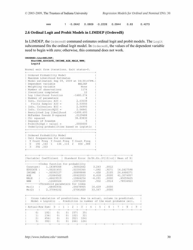
www 1 -0.0642 0.0809 -0.2228 0.0944 0.63 0.4273 2.6 Ordinal Logit and Probit Models in LIMDEP (Ordered$) In LIMDEP, the Ordered$ command estimates ordinal logit and probit models. The Logit subcommand fits the ordinal logit model. In Ordered$, the values of the dependent variable need to begin with zero; otherwise, this command does not work. ORDERED;Lhs=BELIEF; Rhs=ONE,EDUCATE,INCOME,AGE,MALE,WWW; Logit$ Normal exit from iterations. Exit status=0. +---------------------------------------------+ | Ordered Probability Model | | Maximum Likelihood Estimates | | Model estimated: Sep 09, 2009 at 04:30:47PM.| | Dependent variable BELIEF | | Weighting variable None | | Number of observations 1174 | | Iterations completed 12 | | Log likelihood function -1480.274 | | Number of parameters 8 | | Info. Criterion: AIC = 2.53539 | | Finite Sample: AIC = 2.53550 | | Info. Criterion: BIC = 2.56993 | | Info. Criterion:HQIC = 2.54841 | | Restricted log likelihood -1499.693 | | McFadden Pseudo R-squared .0129488 | | Chi squared 38.83830 | | Degrees of freedom 5 | | Prob[ChiSqd > value] = .0000000 | | Underlying probabilities based on Logistic | +---------------------------------------------+ +---------------------------------------------+ | Ordered Probability Model | | Cell frequencies for outcomes | | Y Count Freq Y Count Freq Y Count Freq | | 0 192 .163 1 134 .114 2 456 .388 | | 3 392 .333 | +---------------------------------------------+ +--------+--------------+----------------+--------+--------+----------+ |Variable| Coefficient | Standard Error |b/St.Er.|P[|Z|>z]| Mean of X| +--------+--------------+----------------+--------+--------+----------+ ---------+Index function for probability Constant| 1.18389368 .36502662 3.243 .0012 EDUCATE | -.00201453 .02200365 -.092 .9271 14.2427598 INCOME | -.00592127 .00899848 -.658 .5105 24.6486371 AGE | .01864562 .00422023 4.418 .0000 41.3074957 MALE | -.46619519 .10864254 -4.291 .0000 .45059625 WWW | .12648324 .13572220 .932 .3514 .78534923 ---------+Threshold parameters for index Mu(1) | .68492936 .04678905 14.639 .0000 Mu(2) | 2.37044102 .07061820 33.567 .0000 +---------------------------------------------------------------------------+ | Cross tabulation of predictions. Row is actual, column is predicted. | | Model = Logistic . Prediction is number of the most probable cell. | +-------+-------+-----+-----+-----+-----+-----+-----+-----+-----+-----+-----+ | Actual|Row Sum| 0 | 1 | 2 | 3 | 4 | 5 | 6 | 7 | 8 | 9 | +-------+-------+-----+-----+-----+-----+-----+-----+-----+-----+-----+-----+ | 0| 192| 0| 0| 157| 35| | 1| 134| 0| 0| 102| 32| | 2| 456| 0| 0| 352| 104| | 3| 392| 0| 0| 266| 126| +-------+-------+-----+-----+-----+-----+-----+-----+-----+-----+-----+-----+
© 2003-2009, The Trustees of Indiana University Regression Models for Ordinal and Nominal DVs: 31
http://www.indiana.edu/~statmath 31
|Col Sum| 1174| 0| 0| 877| 297| 0| 0| 0| 0| 0| 0| +-------+-------+-----+-----+-----+-----+-----+-----+-----+-----+-----+-----+
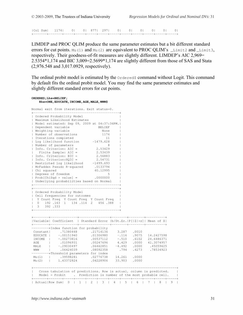
LIMDEP and PROC QLIM produce the same parameter estimates but a bit different standard errors for cut points. Mu(1) and Mu(2) are equivalent to PROC QLIM’s _Limit2 and _Limit3, respectively. Their goodness-of-fit measures are slightly different. LIMDEP’s AIC 2,969= 2.5354*1,174 and BIC 3,009=2.5699*1,174 are slightly different from those of SAS and Stata (2,976.548 and 3,017.0929, respectively). The ordinal probit model is estimated by the Ordered$ command without Logit. This command by default fits the ordinal probit model. You may find the same parameter estimates and slightly different standard errors for cut points. ORDERED;Lhs=BELIEF; Rhs=ONE,EDUCATE,INCOME,AGE,MALE,WWW$ Normal exit from iterations. Exit status=0. +---------------------------------------------+ | Ordered Probability Model | | Maximum Likelihood Estimates | | Model estimated: Sep 09, 2009 at 04:37:36PM.| | Dependent variable BELIEF | | Weighting variable None | | Number of observations 1174 | | Iterations completed 11 | | Log likelihood function -1479.628 | | Number of parameters 8 | | Info. Criterion: AIC = 2.53429 | | Finite Sample: AIC = 2.53439 | | Info. Criterion: BIC = 2.56883 | | Info. Criterion:HQIC = 2.54731 | | Restricted log likelihood -1499.693 | | McFadden Pseudo R-squared .0133794 | | Chi squared 40.12995 | | Degrees of freedom 5 | | Prob[ChiSqd > value] = .0000000 | | Underlying probabilities based on Normal | +---------------------------------------------+ +---------------------------------------------+ | Ordered Probability Model | | Cell frequencies for outcomes | | Y Count Freq Y Count Freq Y Count Freq | | 0 192 .163 1 134 .114 2 456 .388 | | 3 392 .333 | +---------------------------------------------+ +--------+--------------+----------------+--------+--------+----------+ |Variable| Coefficient | Standard Error |b/St.Er.|P[|Z|>z]| Mean of X| +--------+--------------+----------------+--------+--------+----------+ ---------+Index function for probability Constant| .71380448 .21714136 3.287 .0010 EDUCATE | -.00151940 .01306980 -.116 .9075 14.2427598 INCOME | -.00273816 .00537112 -.510 .6102 24.6486371 AGE | .01096931 .00247696 4.429 .0000 41.3074957 MALE | -.29030497 .06462851 -4.492 .0000 .45059625 WWW | .06424039 .08092358 .794 .4273 .78534923 ---------+Threshold parameters for index Mu(1) | .39598281 .02776738 14.261 .0000 Mu(2) | 1.43372824 .04228906 33.903 .0000 +---------------------------------------------------------------------------+ | Cross tabulation of predictions. Row is actual, column is predicted. | | Model = Probit . Prediction is number of the most probable cell. | +-------+-------+-----+-----+-----+-----+-----+-----+-----+-----+-----+-----+ | Actual|Row Sum| 0 | 1 | 2 | 3 | 4 | 5 | 6 | 7 | 8 | 9 |
© 2003-2009, The Trustees of Indiana University Regression Models for Ordinal and Nominal DVs: 32
http://www.indiana.edu/~statmath 32
+-------+-------+-----+-----+-----+-----+-----+-----+-----+-----+-----+-----+ | 0| 192| 0| 0| 158| 34| | 1| 134| 0| 0| 101| 33| | 2| 456| 0| 0| 359| 97| | 3| 392| 0| 0| 265| 127| +-------+-------+-----+-----+-----+-----+-----+-----+-----+-----+-----+-----+ |Col Sum| 1174| 0| 0| 883| 291| 0| 0| 0| 0| 0| 0| +-------+-------+-----+-----+-----+-----+-----+-----+-----+-----+-----+-----+
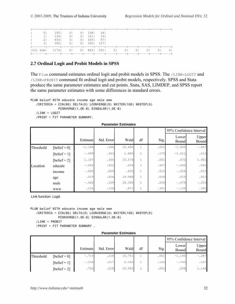
2.7 Ordinal Logit and Probit Models in SPSS The Plum command estimates ordinal logit and probit models in SPSS. The /LINK=LOGIT and /LINK=PROBIT command fit ordinal logit and probit models, respectively. SPSS and Stata produce the same parameter estimates and cut points. Stata, SAS, LIMDEP, and SPSS report the same parameter estimates with some differences in standard errors. PLUM belief WITH educate income age male www /CRITERIA = CIN(95) DELTA(0) LCONVERGE(0) MXITER(100) MXSTEP(5) PCONVERGE(1.0E-6) SINGULAR(1.0E-8) /LINK = LOGIT /PRINT = FIT PARAMETER SUMMARY.
Parameter Estimates
95% Confidence Interval
Estimate Std. Error Wald df Sig.Lower Bound
Upper Bound
[belief = 0] -1.184 .366 10.490 1 .001 -1.900 -.467
[belief = 1] -.499 .363 1.886 1 .170 -1.211 .213
Threshold
[belief = 2] 1.187 .365 10.578 1 .001 .472 1.902
educate -.002 .022 .009 1 .927 -.045 .041
income -.006 .009 .430 1 .512 -.024 .012
age .019 .004 19.988 1 .000 .010 .027
male -.466 .109 18.365 1 .000 -.679 -.253
Location
www .126 .136 .871 1 .351 -.139 .392
Link function: Logit.
PLUM belief WITH educate income age male www /CRITERIA = CIN(95) DELTA(0) LCONVERGE(0) MXITER(100) MXSTEP(5) PCONVERGE(1.0E-6) SINGULAR(1.0E-8) /LINK = PROBIT /PRINT = FIT PARAMETER SUMMARY .
Parameter Estimates
95% Confidence Interval
Estimate Std. Error Wald df Sig.Lower Bound
Upper Bound
[belief = 0] -.714 .218 10.751 1 .001 -1.140 -.287
[belief = 1] -.318 .217 2.145 1 .143 -.743 .107
Threshold
[belief = 2] .720 .218 10.955 1 .001 .294 1.146
© 2003-2009, The Trustees of Indiana University Regression Models for Ordinal and Nominal DVs: 33
http://www.indiana.edu/~statmath 33
educate -.002 .013 .014 1 .907 -.027 .024
income -.003 .005 .259 1 .611 -.013 .008
age .011 .002 19.572 1 .000 .006 .016
male -.290 .065 20.134 1 .000 -.417 -.164
Location
www .064 .081 .631 1 .427 -.094 .223
Link function: Probit.
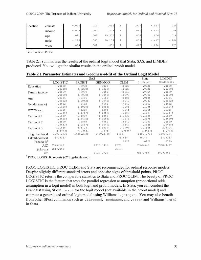
Table 2.1 summarizes the results of the ordinal logit model that Stata, SAS, and LIMDEP produced. You will get the similar results in the ordinal probit model.
Table 2.1 Parameter Estimates and Goodness-of-fit of the Ordinal Logit Model SAS Stata LIMDEP LOGISTIC PROBIT GENMOD QLIM (.ologit) (Ordered$)
Education -.0020 (.0218)
.0020 (.0220)
-.0020 (.0220)
-.0020 (.0220)
-.0020 (.0220)
-.0020 (.0220)
Family income -.0059 (.0090)
.0059 (.0090)
-.0059 (.0090)
-.0059 (.0090)
-.0059 (.0090)
-.0059 (.0090)
Age .0186 (.0042)
-.0186 (.0042)
.0186 (.0042)
.0186 (.0042)
.0186 (.0042)
.0186 (.0042)
Gender (male) -.4662 (.1088)
.4662 (.1085)
-.4662 (.1085)
-.4662 (.1085)
-.4662 (.1085)
-.4662 (.1086)
WWW use .1265 (.1355)
-.1265 (.1357)
.1265 (.1357)
.1265 (.1357)
.1265 (.1357)
.1265 (.1357)
Cut point 1 1.1839 (.3655)
-1.1839 (.3675)
-1.1865 (.3663)
1.1839 (.3675)
-1.1839 (.3675)
1.1839 (.3650)
Cut point 2 .4990 (.3633)
.6849 (.0567)
.4990 (.3649)
.6849 (.0567)
-.4990 (.3649)
.6849 (.0468)
Cut point 3 -1.1865 (.3648)
2.3704 (.0856)
1.1839 (.3675)
2.3704 (.0856)
1.1865 (.3663)
2.3704 (.0762)
Log likelihood -1480.2738 -1480.2738 -1480.2738 -1480. -1480.2738 -1480.274
Likelihood test 38.8383 38.838 38.84 38.8383
Pseudo R2 .0129 .0129 .0129
AIC 2976.548 2976.5475 2977. 2976.548 2968.9417
Schwarz 3017.093 3017.
BIC 3017.0929 3017.093 3009.388 * PROC LOGISTIC reports (-2*Log-likelihood).
PROC LOGISTIC, PROC QLIM, and Stata are recommended for ordinal response models. Despite slightly different standard errors and opposite signs of threshold points, PROC LOGISTIC returns the comparable statistics to Stata and PROC QLIM. The beauty of PROC LOGISTIC is the feature that tests the parallel regression assumption (proportional odds assumption in a logit model) in both logit and probit models. In Stata, you can conduct the Brant test using SPost .brant for the logit model (not available in the probit model) and estimate a generalized ordinal logit model using Williams’ .gologit2. You may also benefit from other SPost commands such as .listcoef, .prchange, and .prgen and Williams’ .mfx2 in Stata.
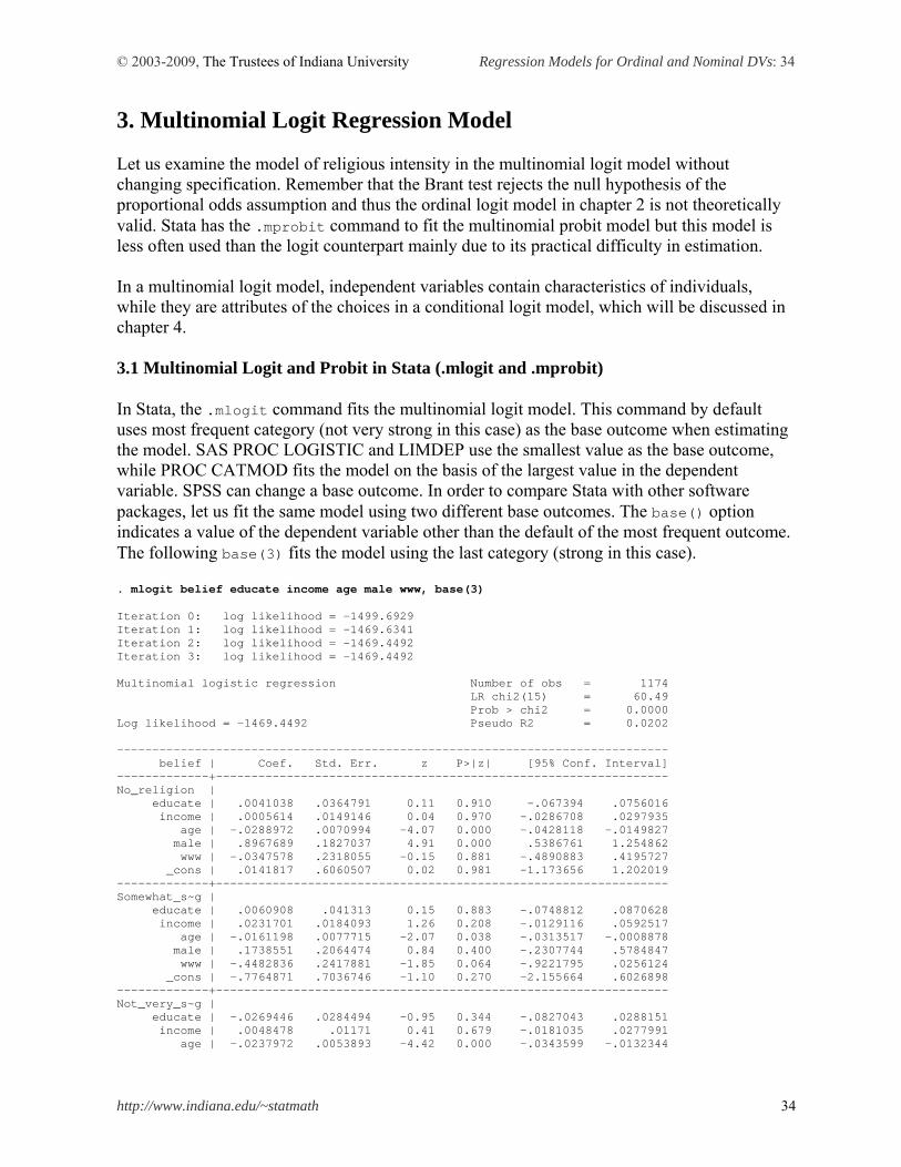
© 2003-2009, The Trustees of Indiana University Regression Models for Ordinal and Nominal DVs: 34
http://www.indiana.edu/~statmath 34
3. Multinomial Logit Regression Model Let us examine the model of religious intensity in the multinomial logit model without changing specification. Remember that the Brant test rejects the null hypothesis of the proportional odds assumption and thus the ordinal logit model in chapter 2 is not theoretically valid. Stata has the .mprobit command to fit the multinomial probit model but this model is less often used than the logit counterpart mainly due to its practical difficulty in estimation. In a multinomial logit model, independent variables contain characteristics of individuals, while they are attributes of the choices in a conditional logit model, which will be discussed in chapter 4. 3.1 Multinomial Logit and Probit in Stata (.mlogit and .mprobit) In Stata, the .mlogit command fits the multinomial logit model. This command by default uses most frequent category (not very strong in this case) as the base outcome when estimating the model. SAS PROC LOGISTIC and LIMDEP use the smallest value as the base outcome, while PROC CATMOD fits the model on the basis of the largest value in the dependent variable. SPSS can change a base outcome. In order to compare Stata with other software packages, let us fit the same model using two different base outcomes. The base() option indicates a value of the dependent variable other than the default of the most frequent outcome. The following base(3) fits the model using the last category (strong in this case). . mlogit belief educate income age male www, base(3) Iteration 0: log likelihood = -1499.6929 Iteration 1: log likelihood = -1469.6341 Iteration 2: log likelihood = -1469.4492 Iteration 3: log likelihood = -1469.4492 Multinomial logistic regression Number of obs = 1174 LR chi2(15) = 60.49 Prob > chi2 = 0.0000 Log likelihood = -1469.4492 Pseudo R2 = 0.0202 ------------------------------------------------------------------------------ belief | Coef. Std. Err. z P>|z| [95% Conf. Interval] -------------+---------------------------------------------------------------- No_religion | educate | .0041038 .0364791 0.11 0.910 -.067394 .0756016 income | .0005614 .0149146 0.04 0.970 -.0286708 .0297935 age | -.0288972 .0070994 -4.07 0.000 -.0428118 -.0149827 male | .8967689 .1827037 4.91 0.000 .5386761 1.254862 www | -.0347578 .2318055 -0.15 0.881 -.4890883 .4195727 _cons | .0141817 .6060507 0.02 0.981 -1.173656 1.202019 -------------+---------------------------------------------------------------- Somewhat_s~g | educate | .0060908 .041313 0.15 0.883 -.0748812 .0870628 income | .0231701 .0184093 1.26 0.208 -.0129116 .0592517 age | -.0161198 .0077715 -2.07 0.038 -.0313517 -.0008878 male | .1738551 .2064474 0.84 0.400 -.2307744 .5784847 www | -.4482836 .2417881 -1.85 0.064 -.9221795 .0256124 _cons | -.7764871 .7036746 -1.10 0.270 -2.155664 .6026898 -------------+---------------------------------------------------------------- Not_very_s~g | educate | -.0269446 .0284494 -0.95 0.344 -.0827043 .0288151 income | .0048478 .01171 0.41 0.679 -.0181035 .0277991 age | -.0237972 .0053893 -4.42 0.000 -.0343599 -.0132344
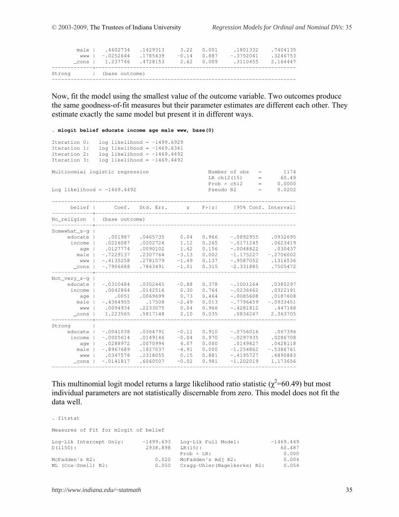
© 2003-2009, The Trustees of Indiana University Regression Models for Ordinal and Nominal DVs: 35
http://www.indiana.edu/~statmath 35
male | .4602734 .1429313 3.22 0.001 .1801332 .7404135 www | -.0252644 .1785439 -0.14 0.887 -.3752041 .3246753 _cons | 1.237746 .4728153 2.62 0.009 .3110455 2.164447 -------------+---------------------------------------------------------------- Strong | (base outcome) ------------------------------------------------------------------------------
Now, fit the model using the smallest value of the outcome variable. Two outcomes produce the same goodness-of-fit measures but their parameter estimates are different each other. They estimate exactly the same model but present it in different ways. . mlogit belief educate income age male www, base(0) Iteration 0: log likelihood = -1499.6929 Iteration 1: log likelihood = -1469.6341 Iteration 2: log likelihood = -1469.4492 Iteration 3: log likelihood = -1469.4492 Multinomial logistic regression Number of obs = 1174 LR chi2(15) = 60.49 Prob > chi2 = 0.0000 Log likelihood = -1469.4492 Pseudo R2 = 0.0202 ------------------------------------------------------------------------------ belief | Coef. Std. Err. z P>|z| [95% Conf. Interval] -------------+---------------------------------------------------------------- No_religion | (base outcome) -------------+---------------------------------------------------------------- Somewhat_s~g | educate | .001987 .0465735 0.04 0.966 -.0892955 .0932695 income | .0226087 .0202724 1.12 0.265 -.0171245 .0623419 age | .0127774 .0090102 1.42 0.156 -.0048822 .030437 male | -.7229137 .2307764 -3.13 0.002 -1.175227 -.2706002 www | -.4135258 .2781579 -1.49 0.137 -.9587052 .1316536 _cons | -.7906688 .7863491 -1.01 0.315 -2.331885 .7505472 -------------+---------------------------------------------------------------- Not_very_s~g | educate | -.0310484 .0352445 -0.88 0.378 -.1001264 .0380297 income | .0042864 .0142516 0.30 0.764 -.0236462 .0322191 age | .0051 .0069699 0.73 0.464 -.0085608 .0187608 male | -.4364955 .17508 -2.49 0.013 -.7796459 -.0933451 www | .0094934 .2233075 0.04 0.966 -.4281812 .447168 _cons | 1.223565 .5817148 2.10 0.035 .0834247 2.363705 -------------+---------------------------------------------------------------- Strong | educate | -.0041038 .0364791 -0.11 0.910 -.0756016 .067394 income | -.0005614 .0149146 -0.04 0.970 -.0297935 .0286708 age | .0288972 .0070994 4.07 0.000 .0149827 .0428118 male | -.8967689 .1827037 -4.91 0.000 -1.254862 -.5386761 www | .0347578 .2318055 0.15 0.881 -.4195727 .4890883 _cons | -.0141817 .6060507 -0.02 0.981 -1.202019 1.173656 ------------------------------------------------------------------------------
This multinomial logit model returns a large likelihood ratio statistic (χ2=60.49) but most individual parameters are not statistically discernable from zero. This model does not fit the data well. . fitstat Measures of Fit for mlogit of belief Log-Lik Intercept Only: -1499.693 Log-Lik Full Model: -1469.449 D(1150): 2938.898 LR(15): 60.487 Prob > LR: 0.000 McFadden's R2: 0.020 McFadden's Adj R2: 0.004 ML (Cox-Snell) R2: 0.050 Cragg-Uhler(Nagelkerke) R2: 0.054
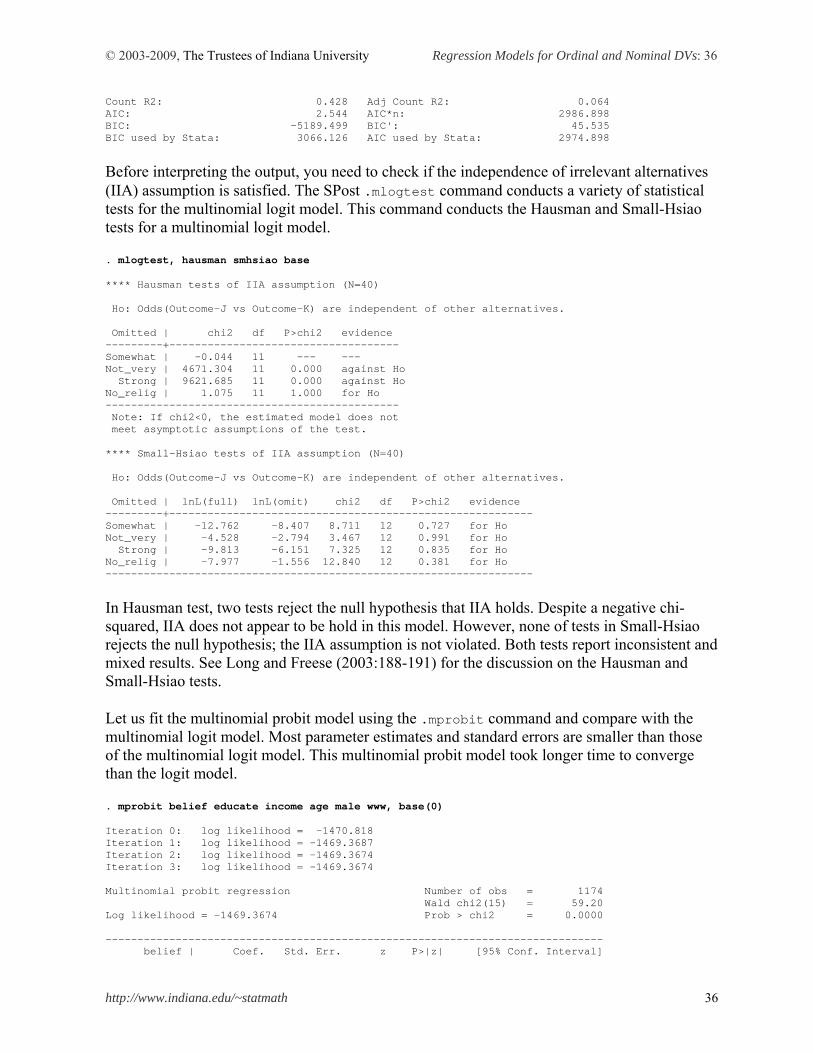
© 2003-2009, The Trustees of Indiana University Regression Models for Ordinal and Nominal DVs: 36
http://www.indiana.edu/~statmath 36
Count R2: 0.428 Adj Count R2: 0.064 AIC: 2.544 AIC*n: 2986.898 BIC: -5189.499 BIC': 45.535 BIC used by Stata: 3066.126 AIC used by Stata: 2974.898
Before interpreting the output, you need to check if the independence of irrelevant alternatives (IIA) assumption is satisfied. The SPost .mlogtest command conducts a variety of statistical tests for the multinomial logit model. This command conducts the Hausman and Small-Hsiao tests for a multinomial logit model. . mlogtest, hausman smhsiao base **** Hausman tests of IIA assumption (N=40) Ho: Odds(Outcome-J vs Outcome-K) are independent of other alternatives. Omitted | chi2 df P>chi2 evidence ---------+------------------------------------ Somewhat | -0.044 11 --- --- Not_very | 4671.304 11 0.000 against Ho Strong | 9621.685 11 0.000 against Ho No_relig | 1.075 11 1.000 for Ho ---------------------------------------------- Note: If chi2<0, the estimated model does not meet asymptotic assumptions of the test. **** Small-Hsiao tests of IIA assumption (N=40) Ho: Odds(Outcome-J vs Outcome-K) are independent of other alternatives. Omitted | lnL(full) lnL(omit) chi2 df P>chi2 evidence ---------+--------------------------------------------------------- Somewhat | -12.762 -8.407 8.711 12 0.727 for Ho Not_very | -4.528 -2.794 3.467 12 0.991 for Ho Strong | -9.813 -6.151 7.325 12 0.835 for Ho No_relig | -7.977 -1.556 12.840 12 0.381 for Ho -------------------------------------------------------------------
In Hausman test, two tests reject the null hypothesis that IIA holds. Despite a negative chi-squared, IIA does not appear to be hold in this model. However, none of tests in Small-Hsiao rejects the null hypothesis; the IIA assumption is not violated. Both tests report inconsistent and mixed results. See Long and Freese (2003:188-191) for the discussion on the Hausman and Small-Hsiao tests. Let us fit the multinomial probit model using the .mprobit command and compare with the multinomial logit model. Most parameter estimates and standard errors are smaller than those of the multinomial logit model. This multinomial probit model took longer time to converge than the logit model. . mprobit belief educate income age male www, base(0) Iteration 0: log likelihood = -1470.818 Iteration 1: log likelihood = -1469.3687 Iteration 2: log likelihood = -1469.3674 Iteration 3: log likelihood = -1469.3674 Multinomial probit regression Number of obs = 1174 Wald chi2(15) = 59.20 Log likelihood = -1469.3674 Prob > chi2 = 0.0000 ------------------------------------------------------------------------------ belief | Coef. Std. Err. z P>|z| [95% Conf. Interval]
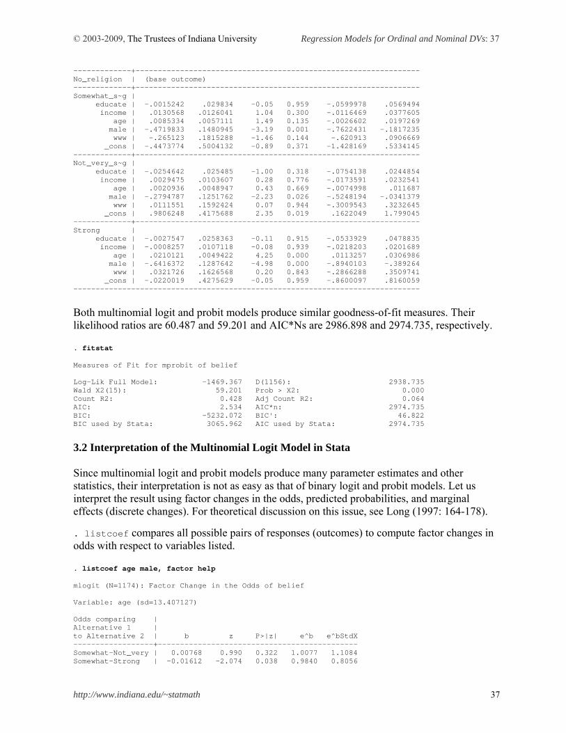
© 2003-2009, The Trustees of Indiana University Regression Models for Ordinal and Nominal DVs: 37
http://www.indiana.edu/~statmath 37
-------------+---------------------------------------------------------------- No_religion | (base outcome) -------------+---------------------------------------------------------------- Somewhat_s~g | educate | -.0015242 .029834 -0.05 0.959 -.0599978 .0569494 income | .0130568 .0126041 1.04 0.300 -.0116469 .0377605 age | .0085334 .0057111 1.49 0.135 -.0026602 .0197269 male | -.4719833 .1480945 -3.19 0.001 -.7622431 -.1817235 www | -.265123 .1815288 -1.46 0.144 -.620913 .0906669 _cons | -.4473774 .5004132 -0.89 0.371 -1.428169 .5334145 -------------+---------------------------------------------------------------- Not_very_s~g | educate | -.0254642 .025485 -1.00 0.318 -.0754138 .0244854 income | .0029475 .0103607 0.28 0.776 -.0173591 .0232541 age | .0020936 .0048947 0.43 0.669 -.0074998 .011687 male | -.2794787 .1251762 -2.23 0.026 -.5248194 -.0341379 www | .0111551 .1592424 0.07 0.944 -.3009543 .3232645 _cons | .9806248 .4175688 2.35 0.019 .1622049 1.799045 -------------+---------------------------------------------------------------- Strong | educate | -.0027547 .0258363 -0.11 0.915 -.0533929 .0478835 income | -.0008257 .0107118 -0.08 0.939 -.0218203 .0201689 age | .0210121 .0049422 4.25 0.000 .0113257 .0306986 male | -.6416372 .1287642 -4.98 0.000 -.8940103 -.389264 www | .0321726 .1626568 0.20 0.843 -.2866288 .3509741 _cons | -.0220019 .4275629 -0.05 0.959 -.8600097 .8160059 ------------------------------------------------------------------------------
Both multinomial logit and probit models produce similar goodness-of-fit measures. Their likelihood ratios are 60.487 and 59.201 and AIC*Ns are 2986.898 and 2974.735, respectively. . fitstat Measures of Fit for mprobit of belief Log-Lik Full Model: -1469.367 D(1156): 2938.735 Wald X2(15): 59.201 Prob > X2: 0.000 Count R2: 0.428 Adj Count R2: 0.064 AIC: 2.534 AIC*n: 2974.735 BIC: -5232.072 BIC': 46.822 BIC used by Stata: 3065.962 AIC used by Stata: 2974.735
3.2 Interpretation of the Multinomial Logit Model in Stata Since multinomial logit and probit models produce many parameter estimates and other statistics, their interpretation is not as easy as that of binary logit and probit models. Let us interpret the result using factor changes in the odds, predicted probabilities, and marginal effects (discrete changes). For theoretical discussion on this issue, see Long (1997: 164-178).
. listcoef compares all possible pairs of responses (outcomes) to compute factor changes in odds with respect to variables listed. . listcoef age male, factor help mlogit (N=1174): Factor Change in the Odds of belief Variable: age (sd=13.407127) Odds comparing | Alternative 1 | to Alternative 2 | b z P>|z| e^b e^bStdX ------------------+--------------------------------------------- Somewhat-Not_very | 0.00768 0.990 0.322 1.0077 1.1084 Somewhat-Strong | -0.01612 -2.074 0.038 0.9840 0.8056
© 2003-2009, The Trustees of Indiana University Regression Models for Ordinal and Nominal DVs: 38
http://www.indiana.edu/~statmath 38
Somewhat-No_relig | 0.01278 1.418 0.156 1.0129 1.1869 Not_very-Somewhat | -0.00768 -0.990 0.322 0.9924 0.9022 Not_very-Strong | -0.02380 -4.416 0.000 0.9765 0.7268 Not_very-No_relig | 0.00510 0.732 0.464 1.0051 1.0708 Strong -Somewhat | 0.01612 2.074 0.038 1.0163 1.2413 Strong -Not_very | 0.02380 4.416 0.000 1.0241 1.3758 Strong -No_relig | 0.02890 4.070 0.000 1.0293 1.4732 No_relig-Somewhat | -0.01278 -1.418 0.156 0.9873 0.8426 No_relig-Not_very | -0.00510 -0.732 0.464 0.9949 0.9339 No_relig-Strong | -0.02890 -4.070 0.000 0.9715 0.6788 ---------------------------------------------------------------- Variable: male (sd=.49776532) Odds comparing | Alternative 1 | to Alternative 2 | b z P>|z| e^b e^bStdX ------------------+--------------------------------------------- Somewhat-Not_very | -0.28642 -1.426 0.154 0.7509 0.8671 Somewhat-Strong | 0.17386 0.842 0.400 1.1899 1.0904 Somewhat-No_relig | -0.72291 -3.133 0.002 0.4853 0.6978 Not_very-Somewhat | 0.28642 1.426 0.154 1.3316 1.1532 Not_very-Strong | 0.46027 3.220 0.001 1.5845 1.2575 Not_very-No_relig | -0.43650 -2.493 0.013 0.6463 0.8047 Strong -Somewhat | -0.17386 -0.842 0.400 0.8404 0.9171 Strong -Not_very | -0.46027 -3.220 0.001 0.6311 0.7952 Strong -No_relig | -0.89677 -4.908 0.000 0.4079 0.6399 No_relig-Somewhat | 0.72291 3.133 0.002 2.0604 1.4331 No_relig-Not_very | 0.43650 2.493 0.013 1.5473 1.2427 No_relig-Strong | 0.89677 4.908 0.000 2.4517 1.5626 ---------------------------------------------------------------- b = raw coefficient z = z-score for test of b=0 P>|z| = p-value for z-test e^b = exp(b) = factor change in odds for unit increase in X e^bStdX = exp(b*SD of X) = change in odds for SD increase in X
Sample interpretations are as follows. For a unit increase in age, the odds of having strong belief (3) versus no religion (0) is expected to increase by a factor of 1.0293=exp(.0289) or the odds of having no religion relative to strong belief will decrease by a factor of .9715=exp(-.0289) =1/1.0293, holding all other variables constant. For a standard deviation increase in age, the odds of having somewhat strong belief (1) relative to not very strong belief (2) will increase by a factor of 1.1084=exp(.0077*13.4071) or the odds of having not very strong belief versus somewhat strong belief is expected to decrease by a factor of .9022= exp(.0077*13.4071)= 1/1.1084. The odds of having strong belief relative to no religion are .4079=exp(-.8968) times smaller for men than for women, holding all other covariates constant; the odds of having no religion relative strong belief are 2.4517 (=1/.4079) times larger for men than for women. Alternative way is to report percent changes of the odds. For a unit increase in age, the odds of having strong belief relative to no religion is expected to increase by 2.9 percent or the odds of having no religion versus strong belief will decrease by 2.8 percent. The odds of having strong belief versus no religion are 59.2 percent smaller for men than for women; the odds of having no religion relative to strong belief are 145.2 percent larger for men than for women. Women are more likely to have religion and, if any, have strong belief than men. . listcoef age male, percent help mlogit (N=1174): Percentage Change in the Odds of belief Variable: age (sd=13.407127)
© 2003-2009, The Trustees of Indiana University Regression Models for Ordinal and Nominal DVs: 39
http://www.indiana.edu/~statmath 39
Odds comparing | Alternative 1 | to Alternative 2 | b z P>|z| % %StdX ------------------+--------------------------------------------- Somewhat-Not_very | 0.00768 0.990 0.322 0.8 10.8 Somewhat-Strong | -0.01612 -2.074 0.038 -1.6 -19.4 Somewhat-No_relig | 0.01278 1.418 0.156 1.3 18.7 Not_very-Somewhat | -0.00768 -0.990 0.322 -0.8 -9.8 Not_very-Strong | -0.02380 -4.416 0.000 -2.4 -27.3 Not_very-No_relig | 0.00510 0.732 0.464 0.5 7.1 Strong -Somewhat | 0.01612 2.074 0.038 1.6 24.1 Strong -Not_very | 0.02380 4.416 0.000 2.4 37.6 Strong -No_relig | 0.02890 4.070 0.000 2.9 47.3 No_relig-Somewhat | -0.01278 -1.418 0.156 -1.3 -15.7 No_relig-Not_very | -0.00510 -0.732 0.464 -0.5 -6.6 No_relig-Strong | -0.02890 -4.070 0.000 -2.8 -32.1 ---------------------------------------------------------------- Variable: male (sd=.49776532) Odds comparing | Alternative 1 | to Alternative 2 | b z P>|z| % %StdX ------------------+--------------------------------------------- Somewhat-Not_very | -0.28642 -1.426 0.154 -24.9 -13.3 Somewhat-Strong | 0.17386 0.842 0.400 19.0 9.0 Somewhat-No_relig | -0.72291 -3.133 0.002 -51.5 -30.2 Not_very-Somewhat | 0.28642 1.426 0.154 33.2 15.3 Not_very-Strong | 0.46027 3.220 0.001 58.5 25.7 Not_very-No_relig | -0.43650 -2.493 0.013 -35.4 -19.5 Strong -Somewhat | -0.17386 -0.842 0.400 -16.0 -8.3 Strong -Not_very | -0.46027 -3.220 0.001 -36.9 -20.5 Strong -No_relig | -0.89677 -4.908 0.000 -59.2 -36.0 No_relig-Somewhat | 0.72291 3.133 0.002 106.0 43.3 No_relig-Not_very | 0.43650 2.493 0.013 54.7 24.3 No_relig-Strong | 0.89677 4.908 0.000 145.2 56.3 ---------------------------------------------------------------- b = raw coefficient z = z-score for test of b=0 P>|z| = p-value for z-test % = percent change in odds for unit increase in X %StdX = percent change in odds for SD increase in X
Predicted probabilities are more intuitive than changes in the odds. You may report predicted probabilities in a table or a plot. .prvalue computes the predicted probabilities of all outcome categories given a set of reference points. For example, the predicted probability that female WWW users with 16 years of education have strong religious belief (belief=3) is 39.41 percent, holding family income and age at their means (25 thousands and age 41). The predicted probability of having no religion is 12.67 percent, 11.61 for somewhat strong, and 36.30 for not very strong. . prvalue, x(educate=16 male=0 www=1) rest(mean) mlogit: Predictions for belief Confidence intervals by delta method 95% Conf. Interval Pr(y=Somewhat|x): 0.1161 [ 0.0871, 0.1451] Pr(y=Not_very|x): 0.3630 [ 0.3193, 0.4068] Pr(y=Strong|x): 0.3941 [ 0.3490, 0.4392] Pr(y=No_relig|x): 0.1267 [ 0.0971, 0.1564] educate income age male www x= 16 24.648637 41.307496 0 1
© 2003-2009, The Trustees of Indiana University Regression Models for Ordinal and Nominal DVs: 40
http://www.indiana.edu/~statmath 40
The following .prtab command returns a series of tables of predicted probabilities for the combination of WWW use and gender. Find the four predicted probabilities above in the following tables. There appear to be significant gender difference in intensity of religious belief but WWW use does not make any significant difference. . prtab male www, x(educate=16 male=0 www=1) rest(mean) mlogit: Predicted probabilities for belief Predicted probability of outcome 1 (Somewhat_strong) -------------------------------- | WWW Use Gender | Non-users Users ----------+--------------------- Female | 0.1684 0.1161 Male | 0.1421 0.0974 -------------------------------- Predicted probability of outcome 2 (Not_very_strong) -------------------------------- | WWW Use Gender | Non-users Users ----------+--------------------- Female | 0.3449 0.3630 Male | 0.3876 0.4056 -------------------------------- Predicted probability of outcome 3 (Strong) -------------------------------- | WWW Use Gender | Non-users Users ----------+--------------------- Female | 0.3651 0.3941 Male | 0.2589 0.2779 -------------------------------- Predicted probability of outcome 0 (No_religion) -------------------------------- | WWW Use Gender | Non-users Users ----------+--------------------- Female | 0.1215 0.1267 Male | 0.2113 0.2191 -------------------------------- educate income age male www x= 16 24.648637 41.307496 0 1
Now, let us see how predicted probabilities change as a continuous covariate increases. The .prgen command makes it easy to generate such predicted probabilities. The following commands generate a series of predicted probabilities that male and female WWW users, who graduated a college, fall in each category of religious intensity at the average family income. . quietly mlogit belief educate income age male www, base(3) . prgen age, from(18) to(92) ncases(20) x(educate=16 male=1 www=1) rest(mean) gen(age1) mlogit: Predicted values as age varies from 18 to 92. educate income age male www x= 16 24.648637 41.307496 1 1
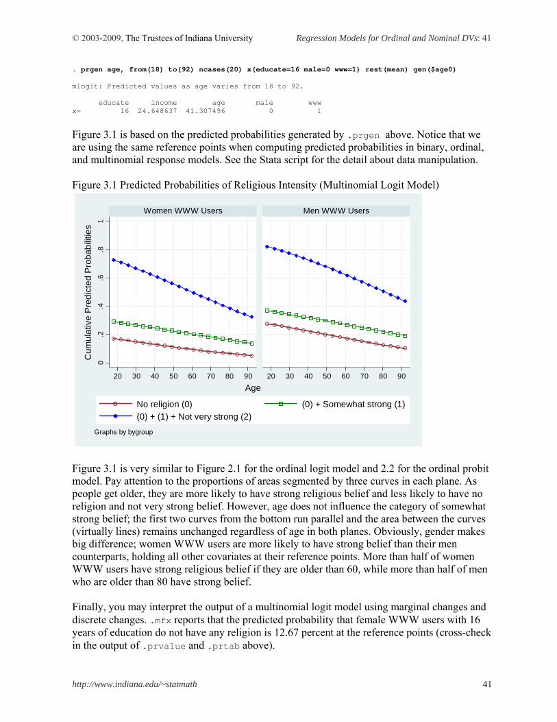
© 2003-2009, The Trustees of Indiana University Regression Models for Ordinal and Nominal DVs: 41
http://www.indiana.edu/~statmath 41
. prgen age, from(18) to(92) ncases(20) x(educate=16 male=0 www=1) rest(mean) gen($age0) mlogit: Predicted values as age varies from 18 to 92. educate income age male www x= 16 24.648637 41.307496 0 1
Figure 3.1 is based on the predicted probabilities generated by .prgen above. Notice that we are using the same reference points when computing predicted probabilities in binary, ordinal, and multinomial response models. See the Stata script for the detail about data manipulation. Figure 3.1 Predicted Probabilities of Religious Intensity (Multinomial Logit Model)
0.2
.4.6
.81
20 30 40 50 60 70 80 90 20 30 40 50 60 70 80 90
Women WWW Users Men WWW Users
No religion (0) (0) + Somewhat strong (1)
(0) + (1) + Not very strong (2)
Cum
ula
tive
Pre
dic
ted
Pro
bab
ilitie
s
Age
Graphs by bygroup
Figure 3.1 is very similar to Figure 2.1 for the ordinal logit model and 2.2 for the ordinal probit model. Pay attention to the proportions of areas segmented by three curves in each plane. As people get older, they are more likely to have strong religious belief and less likely to have no religion and not very strong belief. However, age does not influence the category of somewhat strong belief; the first two curves from the bottom run parallel and the area between the curves (virtually lines) remains unchanged regardless of age in both planes. Obviously, gender makes big difference; women WWW users are more likely to have strong belief than their men counterparts, holding all other covariates at their reference points. More than half of women WWW users have strong religious belief if they are older than 60, while more than half of men who are older than 80 have strong belief. Finally, you may interpret the output of a multinomial logit model using marginal changes and discrete changes. .mfx reports that the predicted probability that female WWW users with 16 years of education do not have any religion is 12.67 percent at the reference points (cross-check in the output of .prvalue and .prtab above).
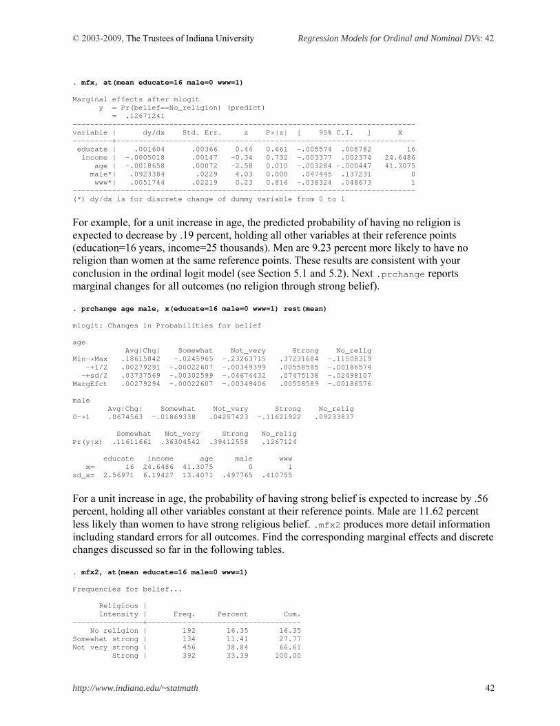
© 2003-2009, The Trustees of Indiana University Regression Models for Ordinal and Nominal DVs: 42
http://www.indiana.edu/~statmath 42
. mfx, at(mean educate=16 male=0 www=1) Marginal effects after mlogit y = Pr(belief==No_religion) (predict) = .12671241 ------------------------------------------------------------------------------ variable | dy/dx Std. Err. z P>|z| [ 95% C.I. ] X ---------+-------------------------------------------------------------------- educate | .001604 .00366 0.44 0.661 -.005574 .008782 16 income | -.0005018 .00147 -0.34 0.732 -.003377 .002374 24.6486 age | -.0018658 .00072 -2.58 0.010 -.003284 -.000447 41.3075 male*| .0923384 .0229 4.03 0.000 .047445 .137231 0 www*| .0051744 .02219 0.23 0.816 -.038324 .048673 1 ------------------------------------------------------------------------------ (*) dy/dx is for discrete change of dummy variable from 0 to 1
For example, for a unit increase in age, the predicted probability of having no religion is expected to decrease by .19 percent, holding all other variables at their reference points (education=16 years, income=25 thousands). Men are 9.23 percent more likely to have no religion than women at the same reference points. These results are consistent with your conclusion in the ordinal logit model (see Section 5.1 and 5.2). Next .prchange reports marginal changes for all outcomes (no religion through strong belief). . prchange age male, x(educate=16 male=0 www=1) rest(mean) mlogit: Changes in Probabilities for belief age Avg|Chg| Somewhat Not_very Strong No_relig Min->Max .18615842 -.0245965 -.23263715 .37231684 -.11508319 -+1/2 .00279291 -.00022607 -.00349399 .00558585 -.00186574 -+sd/2 .03737569 -.00302599 -.04674432 .07475138 -.02498107 MargEfct .00279294 -.00022607 -.00349406 .00558589 -.00186576 male Avg|Chg| Somewhat Not_very Strong No_relig 0->1 .0674563 -.01869338 .04257423 -.11621922 .09233837 Somewhat Not_very Strong No_relig Pr(y|x) .11611661 .36304542 .39412558 .1267124 educate income age male www x= 16 24.6486 41.3075 0 1 sd_x= 2.56971 6.19427 13.4071 .497765 .410755
For a unit increase in age, the probability of having strong belief is expected to increase by .56 percent, holding all other variables constant at their reference points. Male are 11.62 percent less likely than women to have strong religious belief. .mfx2 produces more detail information including standard errors for all outcomes. Find the corresponding marginal effects and discrete changes discussed so far in the following tables. . mfx2, at(mean educate=16 male=0 www=1) Frequencies for belief... Religious | Intensity | Freq. Percent Cum. ----------------+----------------------------------- No religion | 192 16.35 16.35 Somewhat strong | 134 11.41 27.77 Not very strong | 456 38.84 66.61 Strong | 392 33.39 100.00
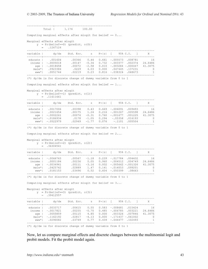
© 2003-2009, The Trustees of Indiana University Regression Models for Ordinal and Nominal DVs: 43
http://www.indiana.edu/~statmath 43
----------------+----------------------------------- Total | 1,174 100.00 Computing marginal effects after mlogit for belief == 0... Marginal effects after mlogit y = Pr(belief==0) (predict, o(0)) = .1267124 ------------------------------------------------------------------------------ variable | dy/dx Std. Err. z P>|z| [ 95% C.I. ] X ---------+-------------------------------------------------------------------- educate | .001604 .00366 0.44 0.661 -.005573 .008781 16 income | -.0005018 .00147 -0.34 0.732 -.003377 .002374 24.6486 age | -.0018658 .00072 -2.58 0.010 -.003284 -.000447 41.3075 male*| .0923384 .0229 4.03 0.000 .047445 .137231 0 www*| .0051744 .02219 0.23 0.816 -.038324 .048673 1 ------------------------------------------------------------------------------ (*) dy/dx is for discrete change of dummy variable from 0 to 1 Computing marginal effects after mlogit for belief == 1... Marginal effects after mlogit y = Pr(belief==1) (predict, o(1)) = .11611661 ------------------------------------------------------------------------------ variable | dy/dx Std. Err. z P>|z| [ 95% C.I. ] X ---------+-------------------------------------------------------------------- educate | .0017006 .00398 0.43 0.669 -.006091 .009493 16 income | .0021654 .00175 1.24 0.216 -.001267 .005598 24.6486 age | -.0002261 .00074 -0.31 0.760 -.001677 .001225 41.3075 male*| -.0186934 .0178 -1.05 0.294 -.05358 .016193 0 www*| -.0522979 .02949 -1.77 0.076 -.1101 .005504 1 ------------------------------------------------------------------------------ (*) dy/dx is for discrete change of dummy variable from 0 to 1 Computing marginal effects after mlogit for belief == 2... Marginal effects after mlogit y = Pr(belief==2) (predict, o(2)) = .36304541 ------------------------------------------------------------------------------ variable | dy/dx Std. Err. z P>|z| [ 95% C.I. ] X ---------+-------------------------------------------------------------------- educate | -.0066763 .00567 -1.18 0.239 -.017784 .004432 16 income | .0001184 .00236 0.05 0.960 -.004512 .004749 24.6486 age | -.0034941 .00111 -3.16 0.002 -.005662 -.001326 41.3075 male*| .0425742 .02889 1.47 0.141 -.014053 .099201 0 www*| .0181153 .03496 0.52 0.604 -.050399 .08663 1 ------------------------------------------------------------------------------ (*) dy/dx is for discrete change of dummy variable from 0 to 1 Computing marginal effects after mlogit for belief == 3... Marginal effects after mlogit y = Pr(belief==3) (predict, o(3)) = .39412557 ------------------------------------------------------------------------------ variable | dy/dx Std. Err. z P>|z| [ 95% C.I. ] X ---------+-------------------------------------------------------------------- educate | .0033717 .00615 0.55 0.583 -.008681 .015424 16 income | -.0017821 .00255 -0.70 0.485 -.006785 .003221 24.6486 age | .0055859 .00115 4.85 0.000 .003326 .007846 41.3075 male*| -.1162192 .02817 -4.13 0.000 -.171437 -.061002 0 www*| .0290082 .03749 0.77 0.439 -.044477 .102493 1 ------------------------------------------------------------------------------ (*) dy/dx is for discrete change of dummy variable from 0 to 1
Now, let us compare marginal effects and discrete changes between the multinomial logit and probit models. Fit the probit model again.
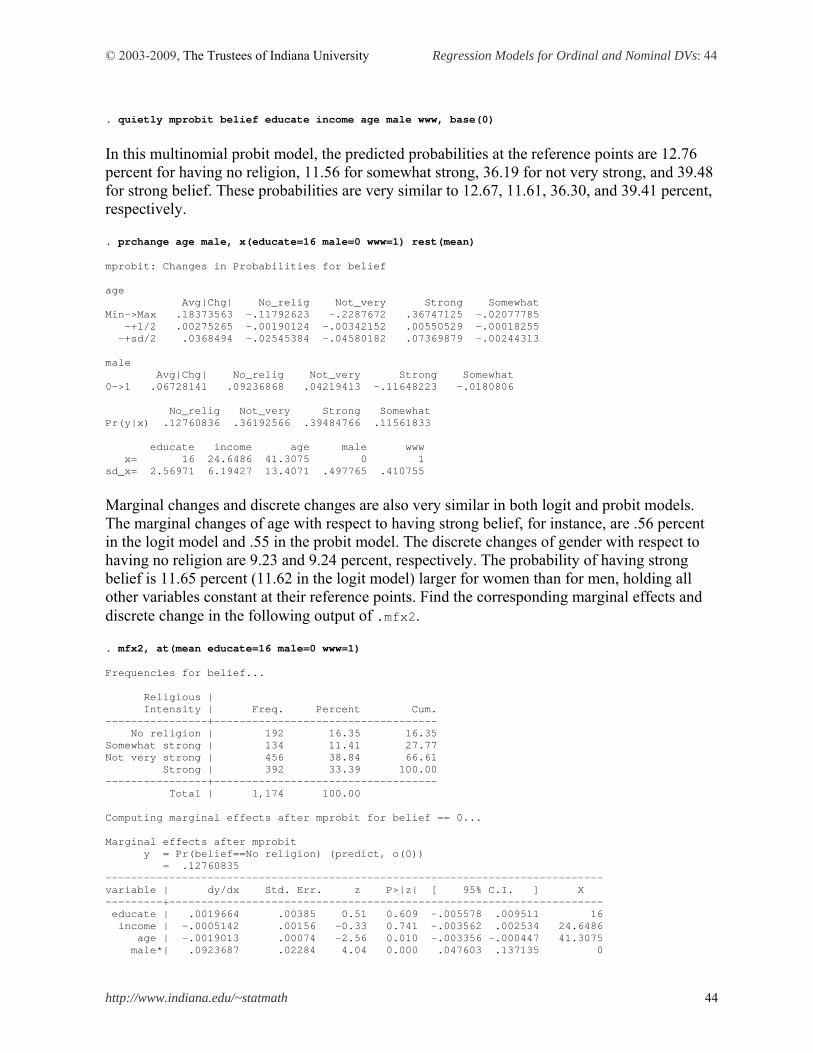
© 2003-2009, The Trustees of Indiana University Regression Models for Ordinal and Nominal DVs: 44
http://www.indiana.edu/~statmath 44
. quietly mprobit belief educate income age male www, base(0)
In this multinomial probit model, the predicted probabilities at the reference points are 12.76 percent for having no religion, 11.56 for somewhat strong, 36.19 for not very strong, and 39.48 for strong belief. These probabilities are very similar to 12.67, 11.61, 36.30, and 39.41 percent, respectively. . prchange age male, x(educate=16 male=0 www=1) rest(mean) mprobit: Changes in Probabilities for belief age Avg|Chg| No_relig Not_very Strong Somewhat Min->Max .18373563 -.11792623 -.2287672 .36747125 -.02077785 -+1/2 .00275265 -.00190124 -.00342152 .00550529 -.00018255 -+sd/2 .0368494 -.02545384 -.04580182 .07369879 -.00244313 male Avg|Chg| No_relig Not_very Strong Somewhat 0->1 .06728141 .09236868 .04219413 -.11648223 -.0180806 No_relig Not_very Strong Somewhat Pr(y|x) .12760836 .36192566 .39484766 .11561833 educate income age male www x= 16 24.6486 41.3075 0 1 sd_x= 2.56971 6.19427 13.4071 .497765 .410755
Marginal changes and discrete changes are also very similar in both logit and probit models. The marginal changes of age with respect to having strong belief, for instance, are .56 percent in the logit model and .55 in the probit model. The discrete changes of gender with respect to having no religion are 9.23 and 9.24 percent, respectively. The probability of having strong belief is 11.65 percent (11.62 in the logit model) larger for women than for men, holding all other variables constant at their reference points. Find the corresponding marginal effects and discrete change in the following output of .mfx2. . mfx2, at(mean educate=16 male=0 www=1) Frequencies for belief... Religious | Intensity | Freq. Percent Cum. ----------------+----------------------------------- No religion | 192 16.35 16.35 Somewhat strong | 134 11.41 27.77 Not very strong | 456 38.84 66.61 Strong | 392 33.39 100.00 ----------------+----------------------------------- Total | 1,174 100.00 Computing marginal effects after mprobit for belief == 0... Marginal effects after mprobit y = Pr(belief==No religion) (predict, o(0)) = .12760835 ------------------------------------------------------------------------------ variable | dy/dx Std. Err. z P>|z| [ 95% C.I. ] X ---------+-------------------------------------------------------------------- educate | .0019664 .00385 0.51 0.609 -.005578 .009511 16 income | -.0005142 .00156 -0.33 0.741 -.003562 .002534 24.6486 age | -.0019013 .00074 -2.56 0.010 -.003356 -.000447 41.3075 male*| .0923687 .02284 4.04 0.000 .047603 .137135 0
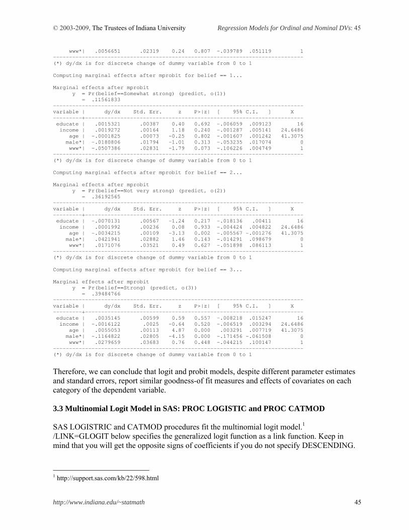
© 2003-2009, The Trustees of Indiana University Regression Models for Ordinal and Nominal DVs: 45
http://www.indiana.edu/~statmath 45
www*| .0056651 .02319 0.24 0.807 -.039789 .051119 1 ------------------------------------------------------------------------------ (*) dy/dx is for discrete change of dummy variable from 0 to 1 Computing marginal effects after mprobit for belief == 1... Marginal effects after mprobit y = Pr(belief==Somewhat strong) (predict, o(1)) = .11561833 ------------------------------------------------------------------------------ variable | dy/dx Std. Err. z P>|z| [ 95% C.I. ] X ---------+-------------------------------------------------------------------- educate | .0015321 .00387 0.40 0.692 -.006059 .009123 16 income | .0019272 .00164 1.18 0.240 -.001287 .005141 24.6486 age | -.0001825 .00073 -0.25 0.802 -.001607 .001242 41.3075 male*| -.0180806 .01794 -1.01 0.313 -.053235 .017074 0 www*| -.0507386 .02831 -1.79 0.073 -.106226 .004749 1 ------------------------------------------------------------------------------ (*) dy/dx is for discrete change of dummy variable from 0 to 1 Computing marginal effects after mprobit for belief == 2... Marginal effects after mprobit y = Pr(belief==Not very strong) (predict, o(2)) = .36192565 ------------------------------------------------------------------------------ variable | dy/dx Std. Err. z P>|z| [ 95% C.I. ] X ---------+-------------------------------------------------------------------- educate | -.0070131 .00567 -1.24 0.217 -.018136 .00411 16 income | .0001992 .00236 0.08 0.933 -.004424 .004822 24.6486 age | -.0034215 .00109 -3.13 0.002 -.005567 -.001276 41.3075 male*| .0421941 .02882 1.46 0.143 -.014291 .098679 0 www*| .0171076 .03521 0.49 0.627 -.051898 .086113 1 ------------------------------------------------------------------------------ (*) dy/dx is for discrete change of dummy variable from 0 to 1 Computing marginal effects after mprobit for belief == 3... Marginal effects after mprobit y = Pr(belief==Strong) (predict, o(3)) = .39484766 ------------------------------------------------------------------------------ variable | dy/dx Std. Err. z P>|z| [ 95% C.I. ] X ---------+-------------------------------------------------------------------- educate | .0035145 .00599 0.59 0.557 -.008218 .015247 16 income | -.0016122 .0025 -0.64 0.520 -.006519 .003294 24.6486 age | .0055053 .00113 4.87 0.000 .003291 .007719 41.3075 male*| -.1164822 .02805 -4.15 0.000 -.171456 -.061508 0 www*| .0279659 .03683 0.76 0.448 -.044215 .100147 1 ------------------------------------------------------------------------------ (*) dy/dx is for discrete change of dummy variable from 0 to 1
Therefore, we can conclude that logit and probit models, despite different parameter estimates and standard errors, report similar goodness-of fit measures and effects of covariates on each category of the dependent variable. 3.3 Multinomial Logit Model in SAS: PROC LOGISTIC and PROC CATMOD SAS LOGISTRIC and CATMOD procedures fit the multinomial logit model.1 /LINK=GLOGIT below specifies the generalized logit function as a link function. Keep in mind that you will get the opposite signs of coefficients if you do not specify DESCENDING.
1 http://support.sas.com/kb/22/598.html
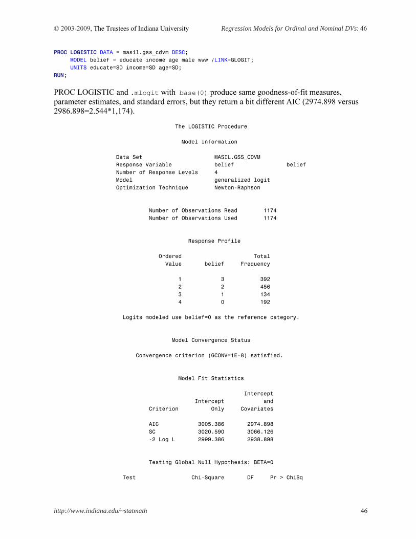
© 2003-2009, The Trustees of Indiana University Regression Models for Ordinal and Nominal DVs: 46
http://www.indiana.edu/~statmath 46
PROC LOGISTIC DATA = masil.gss_cdvm DESC; MODEL belief = educate income age male www /LINK=GLOGIT; UNITS educate=SD income=SD age=SD; RUN;
PROC LOGISTIC and .mlogit with base(0) produce same goodness-of-fit measures, parameter estimates, and standard errors, but they return a bit different AIC (2974.898 versus 2986.898=2.544*1,174). The LOGISTIC Procedure Model Information Data Set MASIL.GSS_CDVM Response Variable belief belief Number of Response Levels 4 Model generalized logit Optimization Technique Newton-Raphson Number of Observations Read 1174 Number of Observations Used 1174 Response Profile Ordered Total Value belief Frequency 1 3 392 2 2 456 3 1 134 4 0 192 Logits modeled use belief=0 as the reference category. Model Convergence Status Convergence criterion (GCONV=1E-8) satisfied. Model Fit Statistics Intercept Intercept and Criterion Only Covariates AIC 3005.386 2974.898 SC 3020.590 3066.126 -2 Log L 2999.386 2938.898 Testing Global Null Hypothesis: BETA=0 Test Chi-Square DF Pr > ChiSq
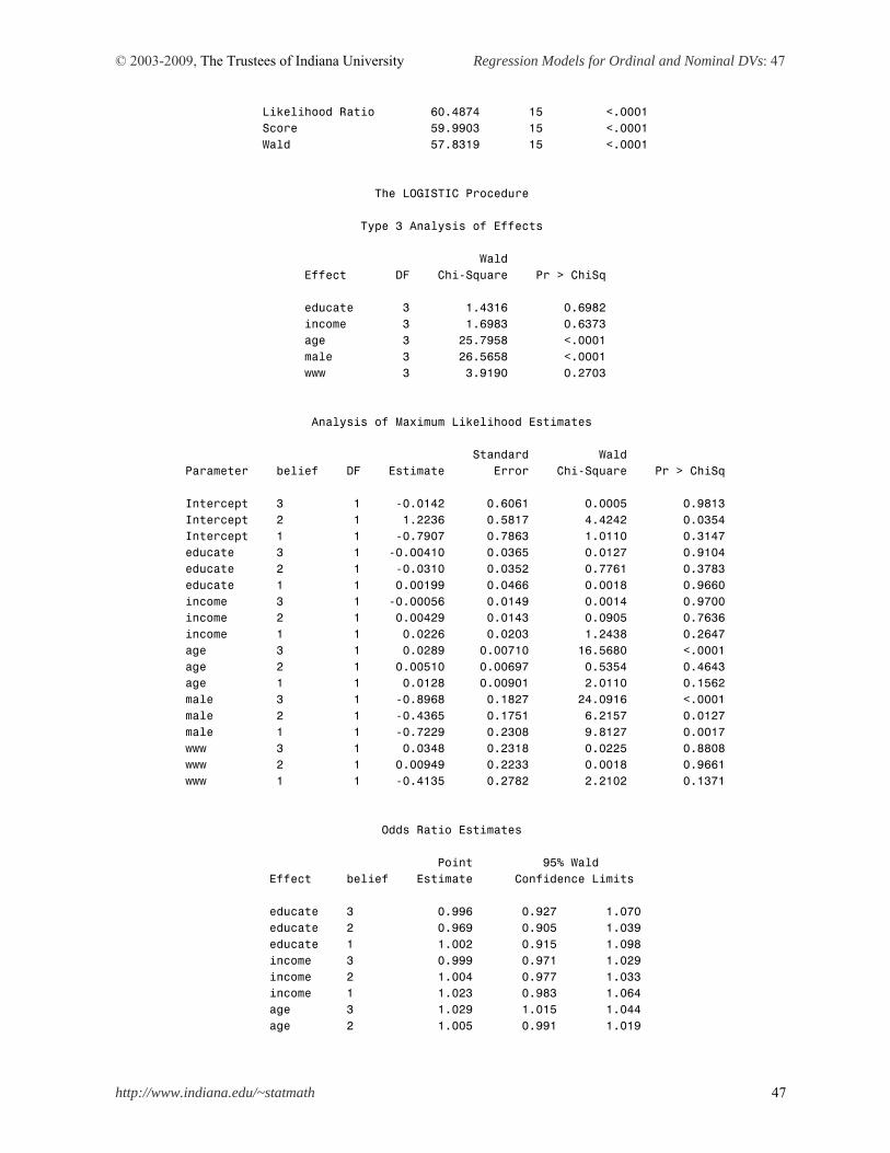
© 2003-2009, The Trustees of Indiana University Regression Models for Ordinal and Nominal DVs: 47
http://www.indiana.edu/~statmath 47
Likelihood Ratio 60.4874 15 <.0001 Score 59.9903 15 <.0001 Wald 57.8319 15 <.0001 The LOGISTIC Procedure Type 3 Analysis of Effects Wald Effect DF Chi-Square Pr > ChiSq educate 3 1.4316 0.6982 income 3 1.6983 0.6373 age 3 25.7958 <.0001 male 3 26.5658 <.0001 www 3 3.9190 0.2703 Analysis of Maximum Likelihood Estimates Standard Wald Parameter belief DF Estimate Error Chi-Square Pr > ChiSq Intercept 3 1 -0.0142 0.6061 0.0005 0.9813 Intercept 2 1 1.2236 0.5817 4.4242 0.0354 Intercept 1 1 -0.7907 0.7863 1.0110 0.3147 educate 3 1 -0.00410 0.0365 0.0127 0.9104 educate 2 1 -0.0310 0.0352 0.7761 0.3783 educate 1 1 0.00199 0.0466 0.0018 0.9660 income 3 1 -0.00056 0.0149 0.0014 0.9700 income 2 1 0.00429 0.0143 0.0905 0.7636 income 1 1 0.0226 0.0203 1.2438 0.2647 age 3 1 0.0289 0.00710 16.5680 <.0001 age 2 1 0.00510 0.00697 0.5354 0.4643 age 1 1 0.0128 0.00901 2.0110 0.1562 male 3 1 -0.8968 0.1827 24.0916 <.0001 male 2 1 -0.4365 0.1751 6.2157 0.0127 male 1 1 -0.7229 0.2308 9.8127 0.0017 www 3 1 0.0348 0.2318 0.0225 0.8808 www 2 1 0.00949 0.2233 0.0018 0.9661 www 1 1 -0.4135 0.2782 2.2102 0.1371 Odds Ratio Estimates Point 95% Wald Effect belief Estimate Confidence Limits educate 3 0.996 0.927 1.070 educate 2 0.969 0.905 1.039 educate 1 1.002 0.915 1.098 income 3 0.999 0.971 1.029 income 2 1.004 0.977 1.033 income 1 1.023 0.983 1.064 age 3 1.029 1.015 1.044 age 2 1.005 0.991 1.019
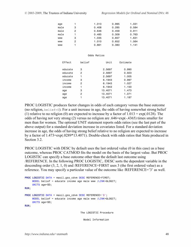
© 2003-2009, The Trustees of Indiana University Regression Models for Ordinal and Nominal DVs: 48
http://www.indiana.edu/~statmath 48
age 1 1.013 0.995 1.031 male 3 0.408 0.285 0.584 male 2 0.646 0.459 0.911 male 1 0.485 0.309 0.763 www 3 1.035 0.657 1.631 www 2 1.010 0.652 1.564 www 1 0.661 0.383 1.141 Odds Ratios Effect belief Unit Estimate educate 3 2.5697 0.990 educate 2 2.5697 0.923 educate 1 2.5697 1.005 income 3 6.1943 0.997 income 2 6.1943 1.027 income 1 6.1943 1.150 age 3 13.4071 1.473 age 2 13.4071 1.071 age 1 13.4071 1.187
PROC LOGISTIC produces factor changes in odds of each category versus the base outcome (no religion, belief=0). For a unit increase in age, the odds of having somewhat strong belief (1) relative to no religion (0) are expected to increase by a factor of 1.013 = exp(.0128). The odds of having not very strong (2) versus no religion are .646=exp(-.4365) times smaller for men than for women. The optional UNIT statement reports odds ratios (see the last part of the above output) for a standard deviation increase in covariates listed. For a standard deviation increase in age, the odds of having strong belief relative to no religion are expected to increase by a factor of 1.473=exp(.0289*13.4071). Double-check with odds ratios that Stata produced in Section 3.2. PROC LOGISTIC with DESC by default uses the last ordered value (0 in this case) as a base outcome, whereas PROC CATMOD fits the model on the basis of the largest value. But PROC LOGISTIC can specify a base outcome other than the default last outcome using /REFERENCE. In the following PROC LOGISTIC, /DESC sorts the dependent variable in the descending order (3, 2, 1, 0) and /REFERENCE=FIRST uses 3 (the first ordered value) as a reference. You may specify a particular value of the outcome like /REFERENCE=’3’ as well. PROC LOGISTIC DATA = masil.gss_cdvm DESC REFERENCE=FIRST; MODEL belief = educate income age male www /LINK=GLOGIT; UNITS age=SD; RUN; PROC LOGISTIC DATA = masil.gss_cdvm DESC REFERENCE='3'; MODEL belief = educate income age male www /LINK=GLOGIT; UNITS age=SD; RUN; The LOGISTIC Procedure Model Information
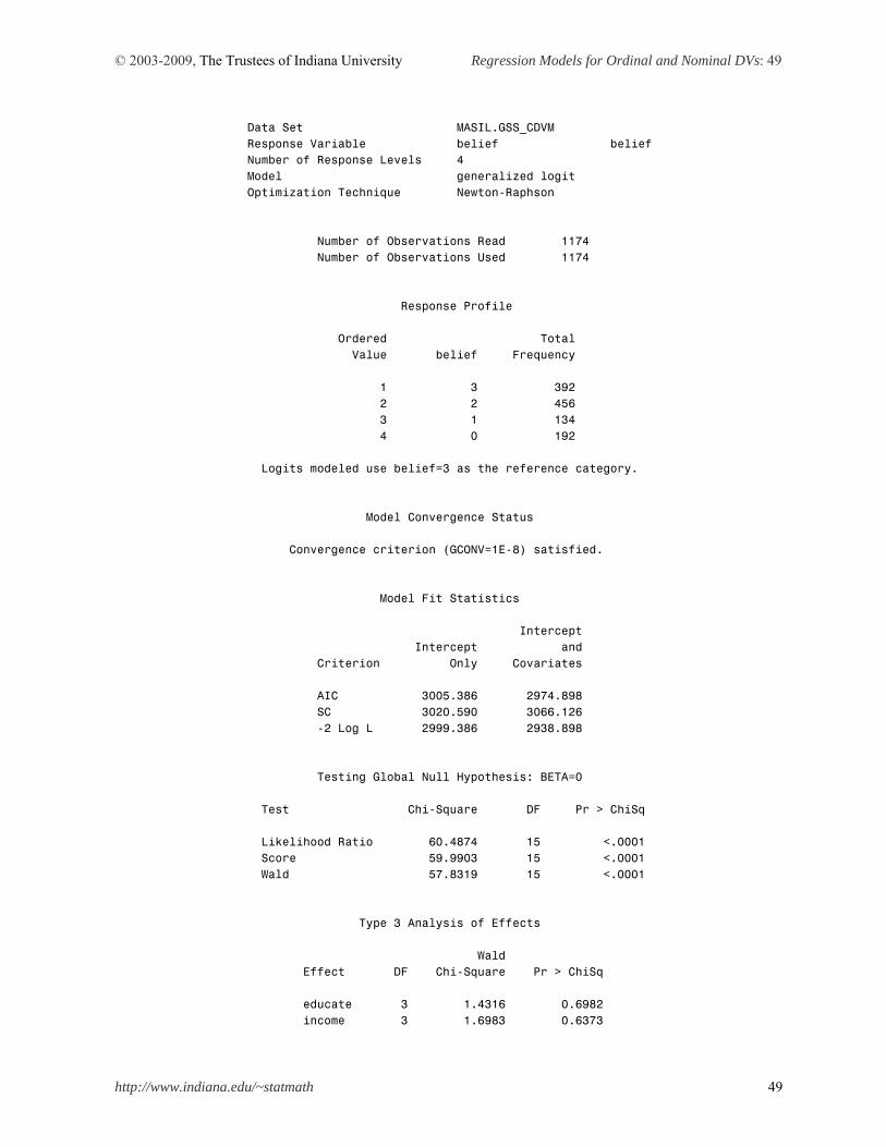
© 2003-2009, The Trustees of Indiana University Regression Models for Ordinal and Nominal DVs: 49
http://www.indiana.edu/~statmath 49
Data Set MASIL.GSS_CDVM Response Variable belief belief Number of Response Levels 4 Model generalized logit Optimization Technique Newton-Raphson Number of Observations Read 1174 Number of Observations Used 1174 Response Profile Ordered Total Value belief Frequency 1 3 392 2 2 456 3 1 134 4 0 192 Logits modeled use belief=3 as the reference category. Model Convergence Status Convergence criterion (GCONV=1E-8) satisfied. Model Fit Statistics Intercept Intercept and Criterion Only Covariates AIC 3005.386 2974.898 SC 3020.590 3066.126 -2 Log L 2999.386 2938.898 Testing Global Null Hypothesis: BETA=0 Test Chi-Square DF Pr > ChiSq Likelihood Ratio 60.4874 15 <.0001 Score 59.9903 15 <.0001 Wald 57.8319 15 <.0001 Type 3 Analysis of Effects Wald Effect DF Chi-Square Pr > ChiSq educate 3 1.4316 0.6982 income 3 1.6983 0.6373
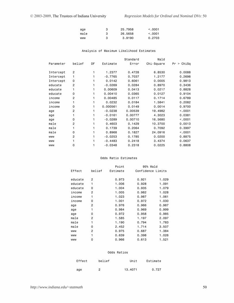
© 2003-2009, The Trustees of Indiana University Regression Models for Ordinal and Nominal DVs: 50
http://www.indiana.edu/~statmath 50
age 3 25.7958 <.0001 male 3 26.5658 <.0001 www 3 3.9190 0.2703 Analysis of Maximum Likelihood Estimates Standard Wald Parameter belief DF Estimate Error Chi-Square Pr > ChiSq Intercept 2 1 1.2377 0.4728 6.8530 0.0088 Intercept 1 1 -0.7765 0.7037 1.2177 0.2698 Intercept 0 1 0.0142 0.6061 0.0005 0.9813 educate 2 1 -0.0269 0.0284 0.8970 0.3436 educate 1 1 0.00609 0.0413 0.0217 0.8828 educate 0 1 0.00410 0.0365 0.0127 0.9104 income 2 1 0.00485 0.0117 0.1714 0.6789 income 1 1 0.0232 0.0184 1.5841 0.2082 income 0 1 0.000561 0.0149 0.0014 0.9700 age 2 1 -0.0238 0.00539 19.4982 <.0001 age 1 1 -0.0161 0.00777 4.3023 0.0381 age 0 1 -0.0289 0.00710 16.5680 <.0001 male 2 1 0.4603 0.1429 10.3700 0.0013 male 1 1 0.1739 0.2064 0.7092 0.3997 male 0 1 0.8968 0.1827 24.0916 <.0001 www 2 1 -0.0253 0.1785 0.0200 0.8875 www 1 1 -0.4483 0.2418 3.4374 0.0637 www 0 1 -0.0348 0.2318 0.0225 0.8808 Odds Ratio Estimates Point 95% Wald Effect belief Estimate Confidence Limits educate 2 0.973 0.921 1.029 educate 1 1.006 0.928 1.091 educate 0 1.004 0.935 1.079 income 2 1.005 0.982 1.028 income 1 1.023 0.987 1.061 income 0 1.001 0.972 1.030 age 2 0.976 0.966 0.987 age 1 0.984 0.969 0.999 age 0 0.972 0.958 0.985 male 2 1.585 1.197 2.097 male 1 1.190 0.794 1.783 male 0 2.452 1.714 3.507 www 2 0.975 0.687 1.384 www 1 0.639 0.398 1.026 www 0 0.966 0.613 1.521 Odds Ratios Effect belief Unit Estimate age 2 13.4071 0.727
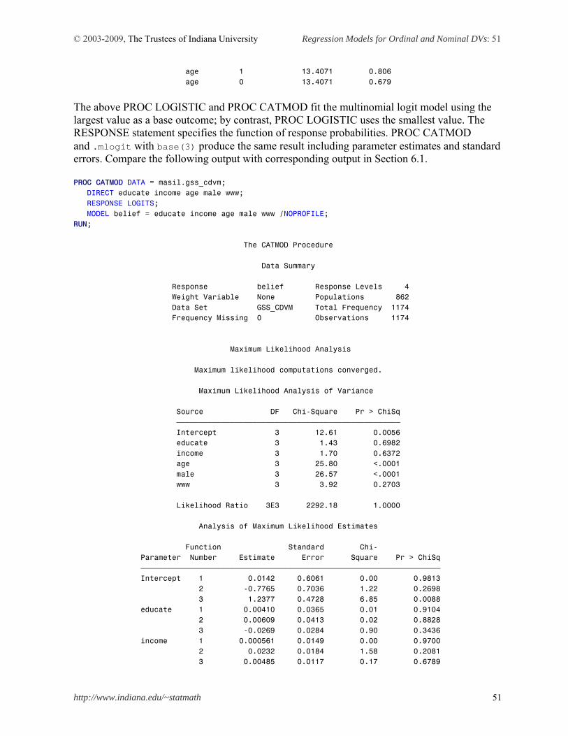
© 2003-2009, The Trustees of Indiana University Regression Models for Ordinal and Nominal DVs: 51
http://www.indiana.edu/~statmath 51
age 1 13.4071 0.806 age 0 13.4071 0.679
The above PROC LOGISTIC and PROC CATMOD fit the multinomial logit model using the largest value as a base outcome; by contrast, PROC LOGISTIC uses the smallest value. The RESPONSE statement specifies the function of response probabilities. PROC CATMOD and .mlogit with base(3) produce the same result including parameter estimates and standard errors. Compare the following output with corresponding output in Section 6.1. PROC CATMOD DATA = masil.gss_cdvm; DIRECT educate income age male www; RESPONSE LOGITS; MODEL belief = educate income age male www /NOPROFILE; RUN; The CATMOD Procedure Data Summary Response belief Response Levels 4 Weight Variable None Populations 862 Data Set GSS_CDVM Total Frequency 1174 Frequency Missing 0 Observations 1174 Maximum Likelihood Analysis Maximum likelihood computations converged. Maximum Likelihood Analysis of Variance Source DF Chi-Square Pr > ChiSq ƒƒƒƒƒƒƒƒƒƒƒƒƒƒƒƒƒƒƒƒƒƒƒƒƒƒƒƒƒƒƒƒƒƒƒƒƒƒƒƒƒƒƒƒƒƒƒƒƒƒ Intercept 3 12.61 0.0056 educate 3 1.43 0.6982 income 3 1.70 0.6372 age 3 25.80 <.0001 male 3 26.57 <.0001 www 3 3.92 0.2703 Likelihood Ratio 3E3 2292.18 1.0000 Analysis of Maximum Likelihood Estimates Function Standard Chi- Parameter Number Estimate Error Square Pr > ChiSq ƒƒƒƒƒƒƒƒƒƒƒƒƒƒƒƒƒƒƒƒƒƒƒƒƒƒƒƒƒƒƒƒƒƒƒƒƒƒƒƒƒƒƒƒƒƒƒƒƒƒƒƒƒƒƒƒƒƒƒƒƒƒƒƒƒƒƒ Intercept 1 0.0142 0.6061 0.00 0.9813 2 -0.7765 0.7036 1.22 0.2698 3 1.2377 0.4728 6.85 0.0088 educate 1 0.00410 0.0365 0.01 0.9104 2 0.00609 0.0413 0.02 0.8828 3 -0.0269 0.0284 0.90 0.3436 income 1 0.000561 0.0149 0.00 0.9700 2 0.0232 0.0184 1.58 0.2081 3 0.00485 0.0117 0.17 0.6789
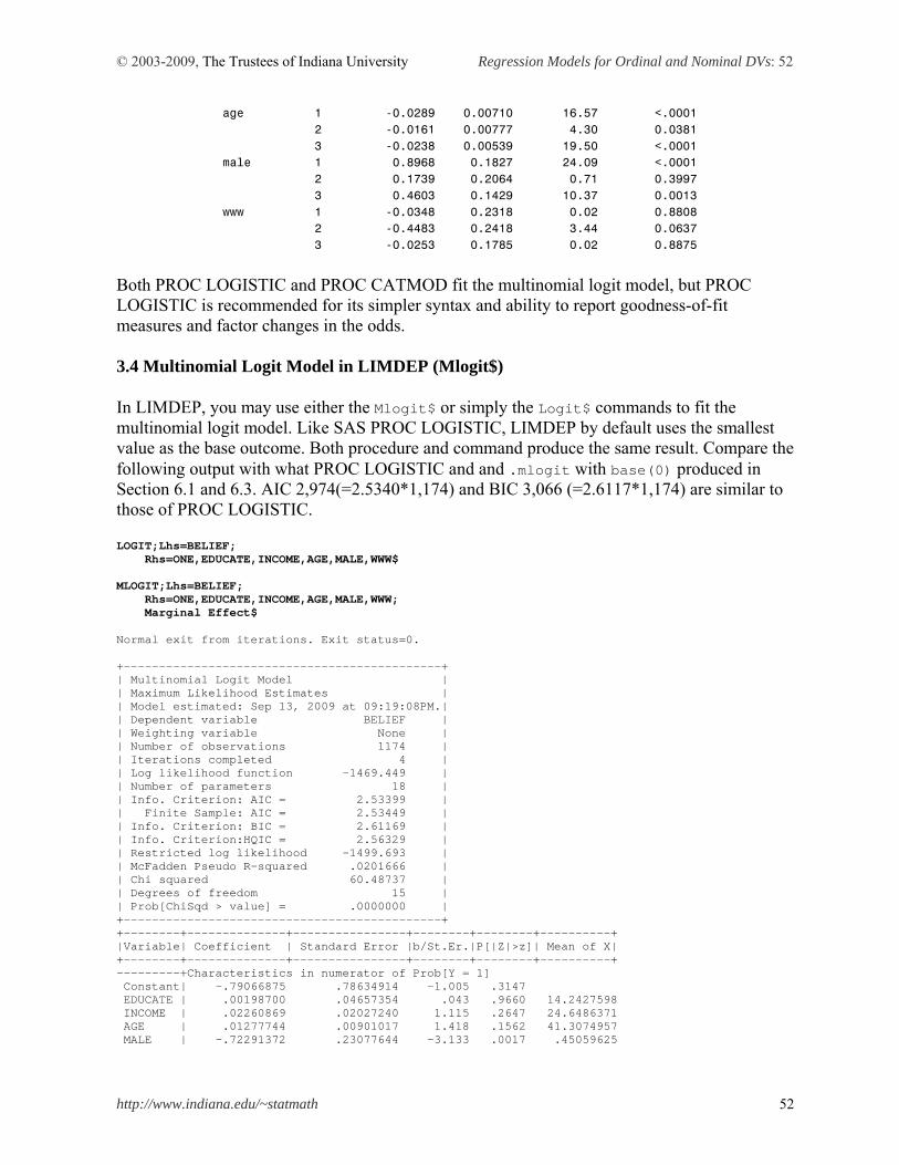
© 2003-2009, The Trustees of Indiana University Regression Models for Ordinal and Nominal DVs: 52
http://www.indiana.edu/~statmath 52
age 1 -0.0289 0.00710 16.57 <.0001 2 -0.0161 0.00777 4.30 0.0381 3 -0.0238 0.00539 19.50 <.0001 male 1 0.8968 0.1827 24.09 <.0001 2 0.1739 0.2064 0.71 0.3997 3 0.4603 0.1429 10.37 0.0013 www 1 -0.0348 0.2318 0.02 0.8808 2 -0.4483 0.2418 3.44 0.0637 3 -0.0253 0.1785 0.02 0.8875
Both PROC LOGISTIC and PROC CATMOD fit the multinomial logit model, but PROC LOGISTIC is recommended for its simpler syntax and ability to report goodness-of-fit measures and factor changes in the odds. 3.4 Multinomial Logit Model in LIMDEP (Mlogit$) In LIMDEP, you may use either the Mlogit$ or simply the Logit$ commands to fit the multinomial logit model. Like SAS PROC LOGISTIC, LIMDEP by default uses the smallest value as the base outcome. Both procedure and command produce the same result. Compare the following output with what PROC LOGISTIC and and .mlogit with base(0) produced in Section 6.1 and 6.3. AIC 2,974(=2.5340*1,174) and BIC 3,066 (=2.6117*1,174) are similar to those of PROC LOGISTIC. LOGIT;Lhs=BELIEF; Rhs=ONE,EDUCATE,INCOME,AGE,MALE,WWW$ MLOGIT;Lhs=BELIEF; Rhs=ONE,EDUCATE,INCOME,AGE,MALE,WWW; Marginal Effect$ Normal exit from iterations. Exit status=0. +---------------------------------------------+ | Multinomial Logit Model | | Maximum Likelihood Estimates | | Model estimated: Sep 13, 2009 at 09:19:08PM.| | Dependent variable BELIEF | | Weighting variable None | | Number of observations 1174 | | Iterations completed 4 | | Log likelihood function -1469.449 | | Number of parameters 18 | | Info. Criterion: AIC = 2.53399 | | Finite Sample: AIC = 2.53449 | | Info. Criterion: BIC = 2.61169 | | Info. Criterion:HQIC = 2.56329 | | Restricted log likelihood -1499.693 | | McFadden Pseudo R-squared .0201666 | | Chi squared 60.48737 | | Degrees of freedom 15 | | Prob[ChiSqd > value] = .0000000 | +---------------------------------------------+ +--------+--------------+----------------+--------+--------+----------+ |Variable| Coefficient | Standard Error |b/St.Er.|P[|Z|>z]| Mean of X| +--------+--------------+----------------+--------+--------+----------+ ---------+Characteristics in numerator of Prob[Y = 1] Constant| -.79066875 .78634914 -1.005 .3147 EDUCATE | .00198700 .04657354 .043 .9660 14.2427598 INCOME | .02260869 .02027240 1.115 .2647 24.6486371 AGE | .01277744 .00901017 1.418 .1562 41.3074957 MALE | -.72291372 .23077644 -3.133 .0017 .45059625
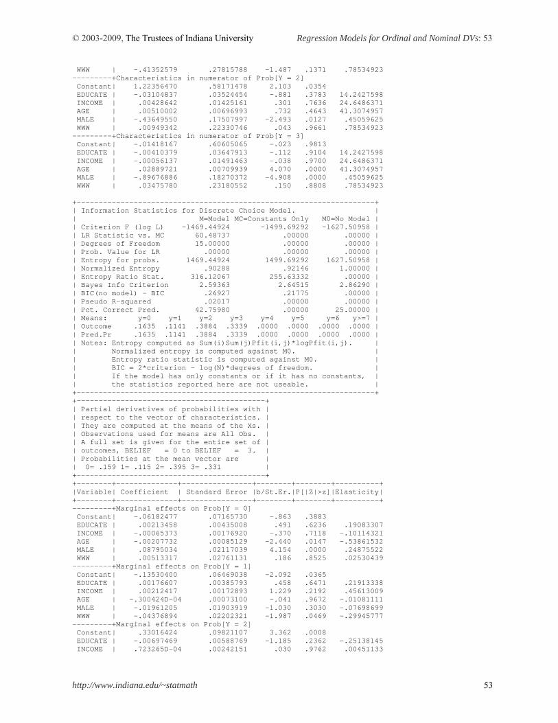
© 2003-2009, The Trustees of Indiana University Regression Models for Ordinal and Nominal DVs: 53
http://www.indiana.edu/~statmath 53
WWW | -.41352579 .27815788 -1.487 .1371 .78534923 ---------+Characteristics in numerator of Prob[Y = 2] Constant| 1.22356470 .58171478 2.103 .0354 EDUCATE | -.03104837 .03524454 -.881 .3783 14.2427598 INCOME | .00428642 .01425161 .301 .7636 24.6486371 AGE | .00510002 .00696993 .732 .4643 41.3074957 MALE | -.43649550 .17507997 -2.493 .0127 .45059625 WWW | .00949342 .22330746 .043 .9661 .78534923 ---------+Characteristics in numerator of Prob[Y = 3] Constant| -.01418167 .60605065 -.023 .9813 EDUCATE | -.00410379 .03647913 -.112 .9104 14.2427598 INCOME | -.00056137 .01491463 -.038 .9700 24.6486371 AGE | .02889721 .00709939 4.070 .0000 41.3074957 MALE | -.89676886 .18270372 -4.908 .0000 .45059625 WWW | .03475780 .23180552 .150 .8808 .78534923 +--------------------------------------------------------------------+ | Information Statistics for Discrete Choice Model. | | M=Model MC=Constants Only M0=No Model | | Criterion F (log L) -1469.44924 -1499.69292 -1627.50958 | | LR Statistic vs. MC 60.48737 .00000 .00000 | | Degrees of Freedom 15.00000 .00000 .00000 | | Prob. Value for LR .00000 .00000 .00000 | | Entropy for probs. 1469.44924 1499.69292 1627.50958 | | Normalized Entropy .90288 .92146 1.00000 | | Entropy Ratio Stat. 316.12067 255.63332 .00000 | | Bayes Info Criterion 2.59363 2.64515 2.86290 | | BIC(no model) - BIC .26927 .21775 .00000 | | Pseudo R-squared .02017 .00000 .00000 | | Pct. Correct Pred. 42.75980 .00000 25.00000 | | Means: y=0 y=1 y=2 y=3 y=4 y=5 y=6 y>=7 | | Outcome .1635 .1141 .3884 .3339 .0000 .0000 .0000 .0000 | | Pred.Pr .1635 .1141 .3884 .3339 .0000 .0000 .0000 .0000 | | Notes: Entropy computed as Sum(i)Sum(j)Pfit(i,j)*logPfit(i,j). | | Normalized entropy is computed against M0. | | Entropy ratio statistic is computed against M0. | | BIC = 2*criterion - log(N)*degrees of freedom. | | If the model has only constants or if it has no constants, | | the statistics reported here are not useable. | +--------------------------------------------------------------------+ +-------------------------------------------+ | Partial derivatives of probabilities with | | respect to the vector of characteristics. | | They are computed at the means of the Xs. | | Observations used for means are All Obs. | | A full set is given for the entire set of | | outcomes, BELIEF = 0 to BELIEF = 3. | | Probabilities at the mean vector are | | 0= .159 1= .115 2= .395 3= .331 | +-------------------------------------------+ +--------+--------------+----------------+--------+--------+----------+ |Variable| Coefficient | Standard Error |b/St.Er.|P[|Z|>z]|Elasticity| +--------+--------------+----------------+--------+--------+----------+ ---------+Marginal effects on Prob[Y = 0] Constant| -.06182477 .07165730 -.863 .3883 EDUCATE | .00213458 .00435008 .491 .6236 .19083307 INCOME | -.00065373 .00176920 -.370 .7118 -.10114321 AGE | -.00207732 .00085129 -2.440 .0147 -.53861532 MALE | .08795034 .02117039 4.154 .0000 .24875522 WWW | .00513317 .02761131 .186 .8525 .02530439 ---------+Marginal effects on Prob[Y = 1] Constant| -.13530400 .06469038 -2.092 .0365 EDUCATE | .00176607 .00385793 .458 .6471 .21913338 INCOME | .00212417 .00172893 1.229 .2192 .45613009 AGE | -.300424D-04 .00073100 -.041 .9672 -.01081111 MALE | -.01961205 .01903919 -1.030 .3030 -.07698699 WWW | -.04376894 .02202321 -1.987 .0469 -.29945777 ---------+Marginal effects on Prob[Y = 2] Constant| .33016424 .09821107 3.362 .0008 EDUCATE | -.00697469 .00588769 -1.185 .2362 -.25138145 INCOME | .723265D-04 .00242151 .030 .9762 .00451133
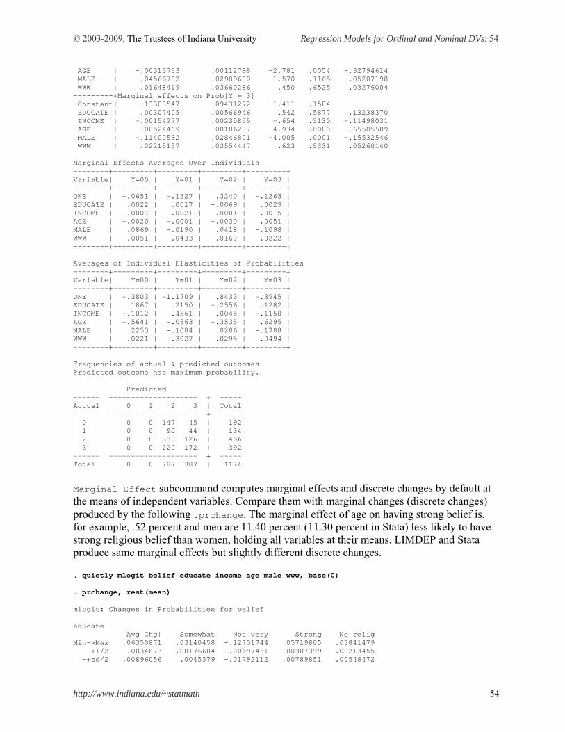
© 2003-2009, The Trustees of Indiana University Regression Models for Ordinal and Nominal DVs: 54
http://www.indiana.edu/~statmath 54
AGE | -.00313733 .00112798 -2.781 .0054 -.32794614 MALE | .04566702 .02909600 1.570 .1165 .05207198 WWW | .01648419 .03660286 .450 .6525 .03276004 ---------+Marginal effects on Prob[Y = 3] Constant| -.13303547 .09431272 -1.411 .1584 EDUCATE | .00307405 .00566946 .542 .5877 .13238370 INCOME | -.00154277 .00235855 -.654 .5130 -.11498031 AGE | .00524469 .00106287 4.934 .0000 .65505589 MALE | -.11400532 .02846801 -4.005 .0001 -.15532546 WWW | .02215157 .03554447 .623 .5331 .05260140 Marginal Effects Averaged Over Individuals --------+---------+---------+---------+---------+ Variable| Y=00 | Y=01 | Y=02 | Y=03 | --------+---------+---------+---------+---------+ ONE | -.0651 | -.1327 | .3240 | -.1263 | EDUCATE | .0022 | .0017 | -.0069 | .0029 | INCOME | -.0007 | .0021 | .0001 | -.0015 | AGE | -.0020 | -.0001 | -.0030 | .0051 | MALE | .0869 | -.0190 | .0418 | -.1098 | WWW | .0051 | -.0433 | .0160 | .0222 | --------+---------+---------+---------+---------+ Averages of Individual Elasticities of Probabilities --------+---------+---------+---------+---------+ Variable| Y=00 | Y=01 | Y=02 | Y=03 | --------+---------+---------+---------+---------+ ONE | -.3803 | -1.1709 | .8433 | -.3945 | EDUCATE | .1867 | .2150 | -.2556 | .1282 | INCOME | -.1012 | .4561 | .0045 | -.1150 | AGE | -.5641 | -.0363 | -.3535 | .6295 | MALE | .2253 | -.1004 | .0286 | -.1788 | WWW | .0221 | -.3027 | .0295 | .0494 | --------+---------+---------+---------+---------+ Frequencies of actual & predicted outcomes Predicted outcome has maximum probability. Predicted ------ -------------------- + ----- Actual 0 1 2 3 | Total ------ -------------------- + ----- 0 0 0 147 45 | 192 1 0 0 90 44 | 134 2 0 0 330 126 | 456 3 0 0 220 172 | 392 ------ -------------------- + ----- Total 0 0 787 387 | 1174
Marginal Effect subcommand computes marginal effects and discrete changes by default at the means of independent variables. Compare them with marginal changes (discrete changes) produced by the following .prchange. The marginal effect of age on having strong belief is, for example, .52 percent and men are 11.40 percent (11.30 percent in Stata) less likely to have strong religious belief than women, holding all variables at their means. LIMDEP and Stata produce same marginal effects but slightly different discrete changes. . quietly mlogit belief educate income age male www, base(0) . prchange, rest(mean) mlogit: Changes in Probabilities for belief educate Avg|Chg| Somewhat Not_very Strong No_relig Min->Max .06350871 .03140458 -.12701744 .05719805 .03841479 -+1/2 .0034873 .00176604 -.00697461 .00307399 .00213455 -+sd/2 .00896056 .0045379 -.01792112 .00789851 .00548472
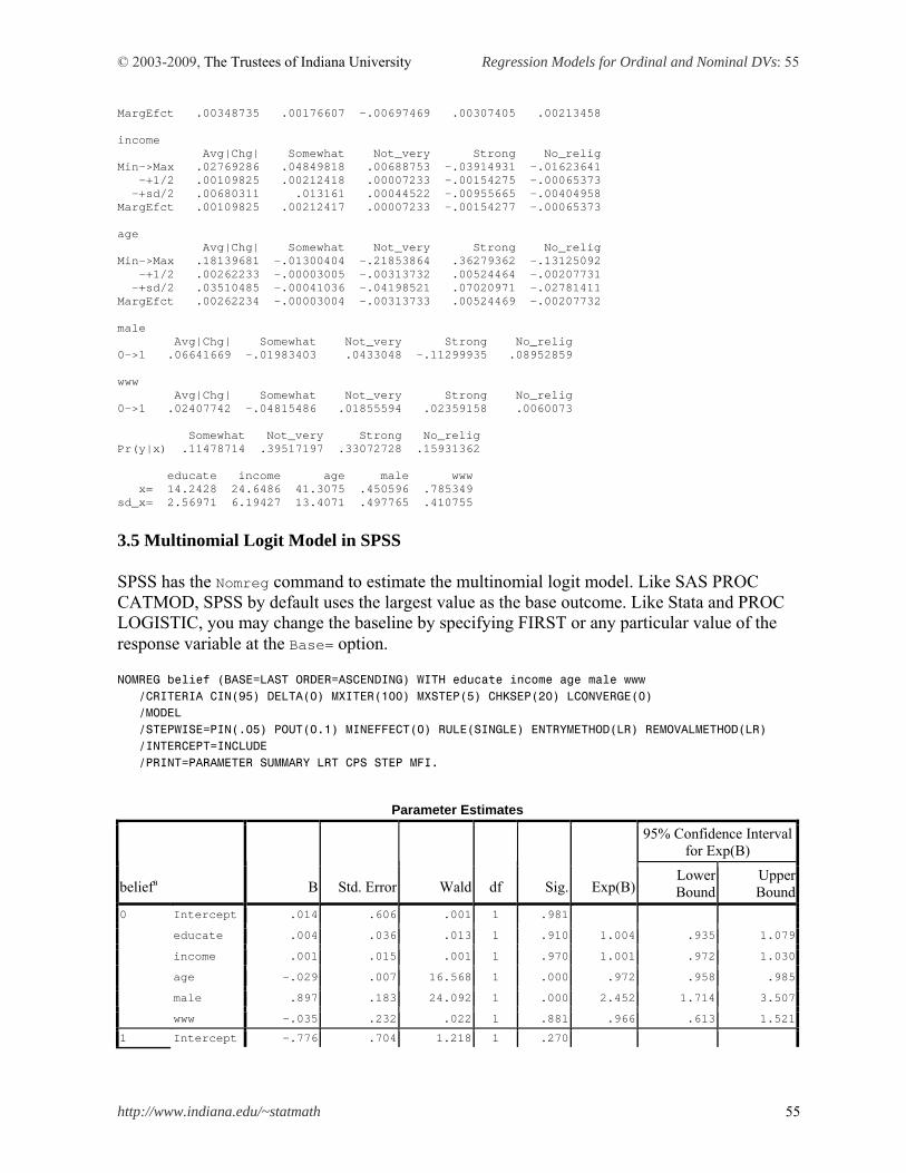
© 2003-2009, The Trustees of Indiana University Regression Models for Ordinal and Nominal DVs: 55
http://www.indiana.edu/~statmath 55
MargEfct .00348735 .00176607 -.00697469 .00307405 .00213458 income Avg|Chg| Somewhat Not_very Strong No_relig Min->Max .02769286 .04849818 .00688753 -.03914931 -.01623641 -+1/2 .00109825 .00212418 .00007233 -.00154275 -.00065373 -+sd/2 .00680311 .013161 .00044522 -.00955665 -.00404958 MargEfct .00109825 .00212417 .00007233 -.00154277 -.00065373 age Avg|Chg| Somewhat Not_very Strong No_relig Min->Max .18139681 -.01300404 -.21853864 .36279362 -.13125092 -+1/2 .00262233 -.00003005 -.00313732 .00524464 -.00207731 -+sd/2 .03510485 -.00041036 -.04198521 .07020971 -.02781411 MargEfct .00262234 -.00003004 -.00313733 .00524469 -.00207732 male Avg|Chg| Somewhat Not_very Strong No_relig 0->1 .06641669 -.01983403 .0433048 -.11299935 .08952859 www Avg|Chg| Somewhat Not_very Strong No_relig 0->1 .02407742 -.04815486 .01855594 .02359158 .0060073 Somewhat Not_very Strong No_relig Pr(y|x) .11478714 .39517197 .33072728 .15931362 educate income age male www x= 14.2428 24.6486 41.3075 .450596 .785349 sd_x= 2.56971 6.19427 13.4071 .497765 .410755
3.5 Multinomial Logit Model in SPSS SPSS has the Nomreg command to estimate the multinomial logit model. Like SAS PROC CATMOD, SPSS by default uses the largest value as the base outcome. Like Stata and PROC LOGISTIC, you may change the baseline by specifying FIRST or any particular value of the response variable at the Base= option. NOMREG belief (BASE=LAST ORDER=ASCENDING) WITH educate income age male www /CRITERIA CIN(95) DELTA(0) MXITER(100) MXSTEP(5) CHKSEP(20) LCONVERGE(0) /MODEL /STEPWISE=PIN(.05) POUT(0.1) MINEFFECT(0) RULE(SINGLE) ENTRYMETHOD(LR) REMOVALMETHOD(LR) /INTERCEPT=INCLUDE /PRINT=PARAMETER SUMMARY LRT CPS STEP MFI.
Parameter Estimates
95% Confidence Interval for Exp(B)
beliefa B Std. Error Wald df Sig. Exp(B)Lower Bound
Upper Bound
Intercept .014 .606 .001 1 .981
educate .004 .036 .013 1 .910 1.004 .935 1.079
income .001 .015 .001 1 .970 1.001 .972 1.030
age -.029 .007 16.568 1 .000 .972 .958 .985
male .897 .183 24.092 1 .000 2.452 1.714 3.507
0
www -.035 .232 .022 1 .881 .966 .613 1.521
1 Intercept -.776 .704 1.218 1 .270
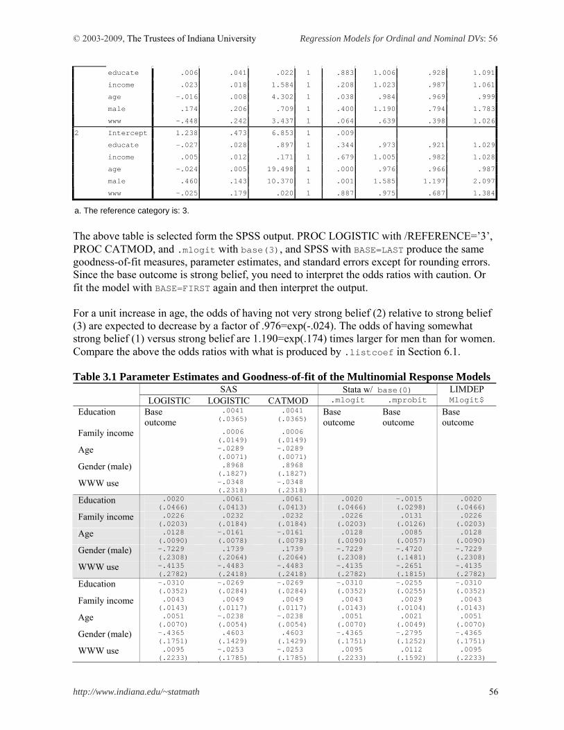
© 2003-2009, The Trustees of Indiana University Regression Models for Ordinal and Nominal DVs: 56
http://www.indiana.edu/~statmath 56
educate .006 .041 .022 1 .883 1.006 .928 1.091
income .023 .018 1.584 1 .208 1.023 .987 1.061
age -.016 .008 4.302 1 .038 .984 .969 .999
male .174 .206 .709 1 .400 1.190 .794 1.783
www -.448 .242 3.437 1 .064 .639 .398 1.026
Intercept 1.238 .473 6.853 1 .009
educate -.027 .028 .897 1 .344 .973 .921 1.029
income .005 .012 .171 1 .679 1.005 .982 1.028
age -.024 .005 19.498 1 .000 .976 .966 .987
male .460 .143 10.370 1 .001 1.585 1.197 2.097
2
www -.025 .179 .020 1 .887 .975 .687 1.384
a. The reference category is: 3.
The above table is selected form the SPSS output. PROC LOGISTIC with /REFERENCE=’3’, PROC CATMOD, and .mlogit with base(3), and SPSS with BASE=LAST produce the same goodness-of-fit measures, parameter estimates, and standard errors except for rounding errors. Since the base outcome is strong belief, you need to interpret the odds ratios with caution. Or fit the model with BASE=FIRST again and then interpret the output. For a unit increase in age, the odds of having not very strong belief (2) relative to strong belief (3) are expected to decrease by a factor of .976=exp(-.024). The odds of having somewhat strong belief (1) versus strong belief are 1.190=exp(.174) times larger for men than for women. Compare the above the odds ratios with what is produced by .listcoef in Section 6.1. Table 3.1 Parameter Estimates and Goodness-of-fit of the Multinomial Response Models
SAS Stata w/ base(0) LIMDEP LOGISTIC LOGISTIC CATMOD .mlogit .mprobit Mlogit$
Education Base outcome
.0041 (.0365)
.0041 (.0365)
Base outcome
Base outcome
Base outcome
Family income .0006 (.0149)
.0006 (.0149)
Age -.0289 (.0071)
-.0289 (.0071)
Gender (male) .8968 (.1827)
.8968 (.1827)
WWW use -.0348 (.2318)
-.0348 (.2318)
Education .0020 (.0466)
.0061 (.0413)
.0061 (.0413)
.0020 (.0466)
-.0015 (.0298)
.0020 (.0466)
Family income .0226 (.0203)
.0232 (.0184)
.0232 (.0184)
.0226 (.0203)
.0131 (.0126)
.0226 (.0203)
Age .0128 (.0090)
-.0161 (.0078)
-.0161 (.0078)
.0128 (.0090)
.0085 (.0057)
.0128 (.0090)
Gender (male) -.7229 (.2308)
.1739 (.2064)
.1739 (.2064)
-.7229 (.2308)
-.4720 (.1481)
-.7229 (.2308)
WWW use -.4135 (.2782)
-.4483 (.2418)
-.4483 (.2418)
-.4135 (.2782)
-.2651 (.1815)
-.4135 (.2782)
Education -.0310 (.0352)
-.0269 (.0284)
-.0269 (.0284)
-.0310 (.0352)
-.0255 (.0255)
-.0310 (.0352)
Family income .0043 (.0143)
.0049 (.0117)
.0049 (.0117)
.0043 (.0143)
.0029 (.0104)
.0043 (.0143)
Age .0051 (.0070)
-.0238 (.0054)
-.0238 (.0054)
.0051 (.0070)
.0021 (.0049)
.0051 (.0070)
Gender (male) -.4365 (.1751)
.4603 (.1429)
.4603 (.1429)
-.4365 (.1751)
-.2795 (.1252)
-.4365 (.1751)
WWW use .0095 (.2233)
-.0253 (.1785)
-.0253 (.1785)
.0095 (.2233)
.0112 (.1592)
.0095 (.2233)
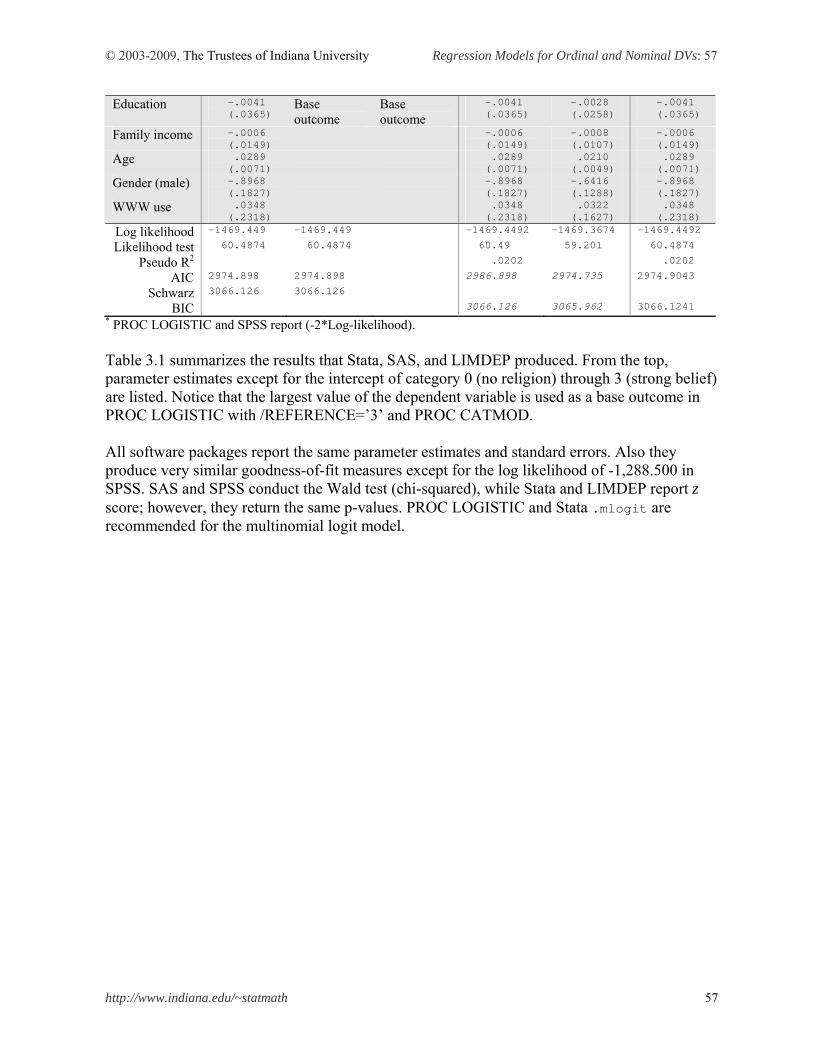
© 2003-2009, The Trustees of Indiana University Regression Models for Ordinal and Nominal DVs: 57
http://www.indiana.edu/~statmath 57
Education -.0041 (.0365)
Base outcome
Base outcome
-.0041 (.0365)
-.0028 (.0258)
-.0041 (.0365)
Family income -.0006 (.0149)
-.0006 (.0149)
-.0008 (.0107)
-.0006 (.0149)
Age .0289 (.0071)
.0289 (.0071)
.0210 (.0049)
.0289 (.0071)
Gender (male) -.8968 (.1827)
-.8968 (.1827)
-.6416 (.1288)
-.8968 (.1827)
WWW use .0348 (.2318)
.0348 (.2318)
.0322 (.1627)
.0348 (.2318)
Log likelihood -1469.449 -1469.449 -1469.4492 -1469.3674 -1469.4492
Likelihood test 60.4874 60.4874 60.49 59.201 60.4874
Pseudo R2 .0202 .0202
AIC 2974.898 2974.898 2986.898 2974.735 2974.9043
Schwarz 3066.126 3066.126
BIC 3066.126 3065.962 3066.1241 * PROC LOGISTIC and SPSS report (-2*Log-likelihood). Table 3.1 summarizes the results that Stata, SAS, and LIMDEP produced. From the top, parameter estimates except for the intercept of category 0 (no religion) through 3 (strong belief) are listed. Notice that the largest value of the dependent variable is used as a base outcome in PROC LOGISTIC with /REFERENCE=’3’ and PROC CATMOD. All software packages report the same parameter estimates and standard errors. Also they produce very similar goodness-of-fit measures except for the log likelihood of -1,288.500 in SPSS. SAS and SPSS conduct the Wald test (chi-squared), while Stata and LIMDEP report z score; however, they return the same p-values. PROC LOGISTIC and Stata .mlogit are recommended for the multinomial logit model.
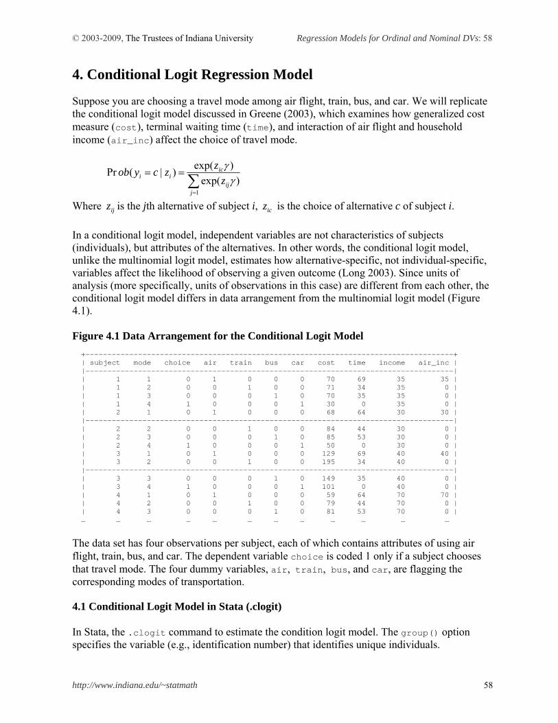
© 2003-2009, The Trustees of Indiana University Regression Models for Ordinal and Nominal DVs: 58
http://www.indiana.edu/~statmath 58
4. Conditional Logit Regression Model Suppose you are choosing a travel mode among air flight, train, bus, and car. We will replicate the conditional logit model discussed in Greene (2003), which examines how generalized cost measure (cost), terminal waiting time (time), and interaction of air flight and household income (air_inc) affect the choice of travel mode.
1
)exp(
)exp()|(Pr
jij
icii z
zzcyob
Where ijz is the jth alternative of subject i, icz is the choice of alternative c of subject i.
In a conditional logit model, independent variables are not characteristics of subjects (individuals), but attributes of the alternatives. In other words, the conditional logit model, unlike the multinomial logit model, estimates how alternative-specific, not individual-specific, variables affect the likelihood of observing a given outcome (Long 2003). Since units of analysis (more specifically, units of observations in this case) are different from each other, the conditional logit model differs in data arrangement from the multinomial logit model (Figure 4.1). Figure 4.1 Data Arrangement for the Conditional Logit Model +------------------------------------------------------------------------------------+ | subject mode choice air train bus car cost time income air_inc | |------------------------------------------------------------------------------------| | 1 1 0 1 0 0 0 70 69 35 35 | | 1 2 0 0 1 0 0 71 34 35 0 | | 1 3 0 0 0 1 0 70 35 35 0 | | 1 4 1 0 0 0 1 30 0 35 0 | | 2 1 0 1 0 0 0 68 64 30 30 | |------------------------------------------------------------------------------------| | 2 2 0 0 1 0 0 84 44 30 0 | | 2 3 0 0 0 1 0 85 53 30 0 | | 2 4 1 0 0 0 1 50 0 30 0 | | 3 1 0 1 0 0 0 129 69 40 40 | | 3 2 0 0 1 0 0 195 34 40 0 | |------------------------------------------------------------------------------------| | 3 3 0 0 0 1 0 149 35 40 0 | | 3 4 1 0 0 0 1 101 0 40 0 | | 4 1 0 1 0 0 0 59 64 70 70 | | 4 2 0 0 1 0 0 79 44 70 0 | | 4 3 0 0 0 1 0 81 53 70 0 | … … … … … … … … … … … …
The data set has four observations per subject, each of which contains attributes of using air flight, train, bus, and car. The dependent variable choice is coded 1 only if a subject chooses that travel mode. The four dummy variables, air, train, bus, and car, are flagging the corresponding modes of transportation. 4.1 Conditional Logit Model in Stata (.clogit) In Stata, the .clogit command to estimate the condition logit model. The group() option specifies the variable (e.g., identification number) that identifies unique individuals.
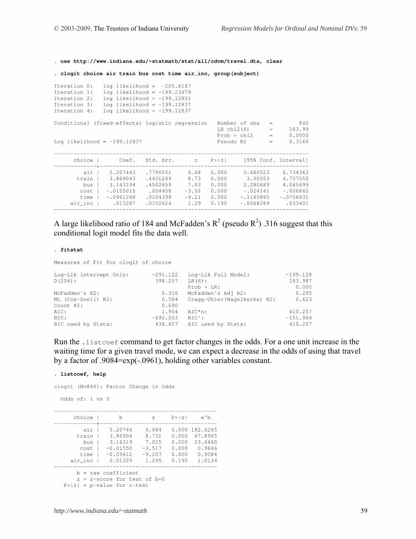
© 2003-2009, The Trustees of Indiana University Regression Models for Ordinal and Nominal DVs: 59
http://www.indiana.edu/~statmath 59
. use http://www.indiana.edu/~statmath/stat/all/cdvm/travel.dta, clear . clogit choice air train bus cost time air_inc, group(subject) Iteration 0: log likelihood = -205.8187 Iteration 1: log likelihood = -199.23679 Iteration 2: log likelihood = -199.12851 Iteration 3: log likelihood = -199.12837 Iteration 4: log likelihood = -199.12837 Conditional (fixed-effects) logistic regression Number of obs = 840 LR chi2(6) = 183.99 Prob > chi2 = 0.0000 Log likelihood = -199.12837 Pseudo R2 = 0.3160 ------------------------------------------------------------------------------ choice | Coef. Std. Err. z P>|z| [95% Conf. Interval] -------------+---------------------------------------------------------------- air | 5.207443 .7790551 6.68 0.000 3.680523 6.734363 train | 3.869043 .4431269 8.73 0.000 3.00053 4.737555 bus | 3.163194 .4502659 7.03 0.000 2.280689 4.045699 cost | -.0155015 .004408 -3.52 0.000 -.024141 -.006862 time | -.0961248 .0104398 -9.21 0.000 -.1165865 -.0756631 air_inc | .013287 .0102624 1.29 0.195 -.0068269 .033401 ------------------------------------------------------------------------------
A large likelihood ratio of 184 and McFadden’s R2 (pseudo R2) .316 suggest that this conditional logit model fits the data well. . fitstat Measures of Fit for clogit of choice Log-Lik Intercept Only: -291.122 Log-Lik Full Model: -199.128 D(204): 398.257 LR(6): 183.987 Prob > LR: 0.000 McFadden's R2: 0.316 McFadden's Adj R2: 0.295 ML (Cox-Snell) R2: 0.584 Cragg-Uhler(Nagelkerke) R2: 0.623 Count R2: 0.690 AIC: 1.954 AIC*n: 410.257 BIC: -692.553 BIC': -151.904 BIC used by Stata: 438.657 AIC used by Stata: 410.257
Run the .listcoef command to get factor changes in the odds. For a one unit increase in the waiting time for a given travel mode, we can expect a decrease in the odds of using that travel by a factor of .9084=exp(-.0961), holding other variables constant. . listcoef, help clogit (N=840): Factor Change in Odds Odds of: 1 vs 0 -------------------------------------------------- choice | b z P>|z| e^b -------------+------------------------------------ air | 5.20744 6.684 0.000 182.6265 train | 3.86904 8.731 0.000 47.8965 bus | 3.16319 7.025 0.000 23.6460 cost | -0.01550 -3.517 0.000 0.9846 time | -0.09612 -9.207 0.000 0.9084 air_inc | 0.01329 1.295 0.195 1.0134 -------------------------------------------------- b = raw coefficient z = z-score for test of b=0 P>|z| = p-value for z-test
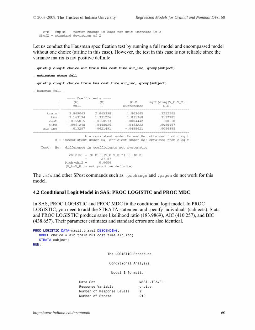
© 2003-2009, The Trustees of Indiana University Regression Models for Ordinal and Nominal DVs: 60
http://www.indiana.edu/~statmath 60
e^b = exp(b) = factor change in odds for unit increase in X SDofX = standard deviation of X
Let us conduct the Hausman specification test by running a full model and encompassed model without one choice (airline in this case). However, the test in this case is not reliable since the variance matrix is not positive definite . quietly clogit choice air train bus cost time air_inc, group(subject) . estimates store full . quietly clogit choice train bus cost time air_inc, group(subject) . hausman full . ---- Coefficients ---- | (b) (B) (b-B) sqrt(diag(V_b-V_B)) | full . Difference S.E. -------------+---------------------------------------------------------------- train | 3.869043 2.065398 1.803645 .3252505 bus | 3.163194 1.331226 1.831968 .3137705 cost | -.0155015 -.0150573 -.0004442 .00118 time | -.0961248 -.0498026 -.0463222 .0080997 air_inc | .013287 .0621491 -.0488621 .0056885 ------------------------------------------------------------------------------ b = consistent under Ho and Ha; obtained from clogit B = inconsistent under Ha, efficient under Ho; obtained from clogit Test: Ho: difference in coefficients not systematic chi2(5) = (b-B)'[(V_b-V_B)^(-1)](b-B) = 27.87 Prob>chi2 = 0.0000 (V_b-V_B is not positive definite)
The .mfx and other SPost commands such as .prchange and .prgen do not work for this model. 4.2 Conditional Logit Model in SAS: PROC LOGISTIC and PROC MDC In SAS, PROC LOGISTIC and PROC MDC fit the conditional logit model. In PROC LOGISTIC, you need to add the STRATA statement and specify individuals (subjects). Stata and PROC LOGISTIC produce same likelihood ratio (183.9869), AIC (410.257), and BIC (438.657). Their parameter estimates and standard errors are also identical. PROC LOGISTIC DATA=masil.travel DESCENDING; MODEL choice = air train bus cost time air_inc; STRATA subject; RUN; The LOGISTIC Procedure Conditional Analysis Model Information Data Set MASIL.TRAVEL Response Variable choice Number of Response Levels 2 Number of Strata 210
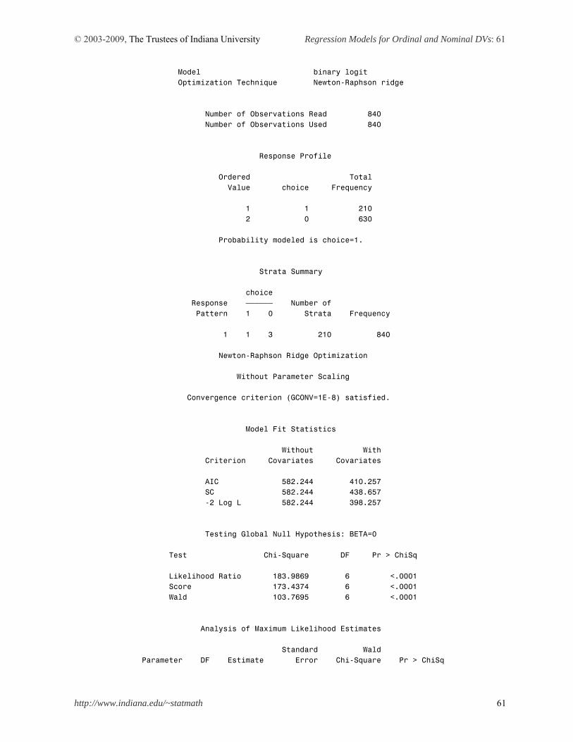
© 2003-2009, The Trustees of Indiana University Regression Models for Ordinal and Nominal DVs: 61
http://www.indiana.edu/~statmath 61
Model binary logit Optimization Technique Newton-Raphson ridge Number of Observations Read 840 Number of Observations Used 840 Response Profile Ordered Total Value choice Frequency 1 1 210 2 0 630 Probability modeled is choice=1. Strata Summary choice Response ƒƒƒƒƒƒ Number of Pattern 1 0 Strata Frequency 1 1 3 210 840 Newton-Raphson Ridge Optimization Without Parameter Scaling Convergence criterion (GCONV=1E-8) satisfied. Model Fit Statistics Without With Criterion Covariates Covariates AIC 582.244 410.257 SC 582.244 438.657 -2 Log L 582.244 398.257 Testing Global Null Hypothesis: BETA=0 Test Chi-Square DF Pr > ChiSq Likelihood Ratio 183.9869 6 <.0001 Score 173.4374 6 <.0001 Wald 103.7695 6 <.0001 Analysis of Maximum Likelihood Estimates Standard Wald Parameter DF Estimate Error Chi-Square Pr > ChiSq
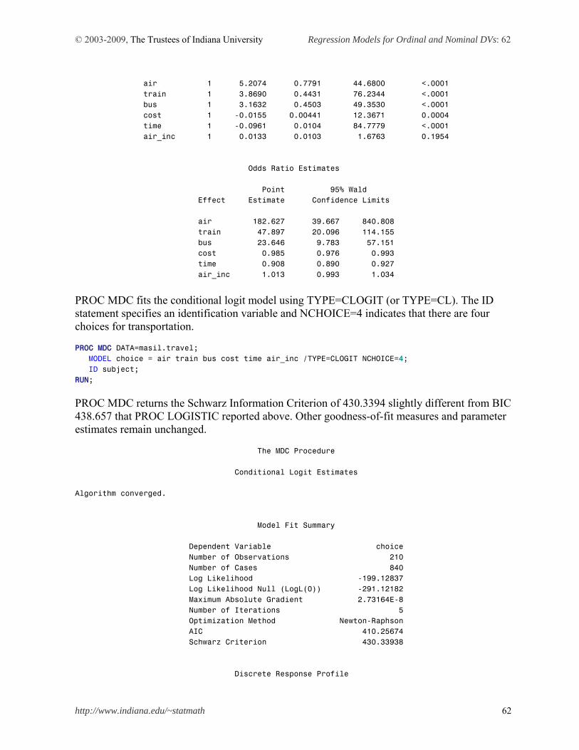
© 2003-2009, The Trustees of Indiana University Regression Models for Ordinal and Nominal DVs: 62
http://www.indiana.edu/~statmath 62
air 1 5.2074 0.7791 44.6800 <.0001 train 1 3.8690 0.4431 76.2344 <.0001 bus 1 3.1632 0.4503 49.3530 <.0001 cost 1 -0.0155 0.00441 12.3671 0.0004 time 1 -0.0961 0.0104 84.7779 <.0001 air_inc 1 0.0133 0.0103 1.6763 0.1954 Odds Ratio Estimates Point 95% Wald Effect Estimate Confidence Limits air 182.627 39.667 840.808 train 47.897 20.096 114.155 bus 23.646 9.783 57.151 cost 0.985 0.976 0.993 time 0.908 0.890 0.927 air_inc 1.013 0.993 1.034
PROC MDC fits the conditional logit model using TYPE=CLOGIT (or TYPE=CL). The ID statement specifies an identification variable and NCHOICE=4 indicates that there are four choices for transportation. PROC MDC DATA=masil.travel; MODEL choice = air train bus cost time air_inc /TYPE=CLOGIT NCHOICE=4; ID subject; RUN;
PROC MDC returns the Schwarz Information Criterion of 430.3394 slightly different from BIC 438.657 that PROC LOGISTIC reported above. Other goodness-of-fit measures and parameter estimates remain unchanged. The MDC Procedure Conditional Logit Estimates Algorithm converged. Model Fit Summary Dependent Variable choice Number of Observations 210 Number of Cases 840 Log Likelihood -199.12837 Log Likelihood Null (LogL(0)) -291.12182 Maximum Absolute Gradient 2.73164E-8 Number of Iterations 5 Optimization Method Newton-Raphson AIC 410.25674 Schwarz Criterion 430.33938 Discrete Response Profile
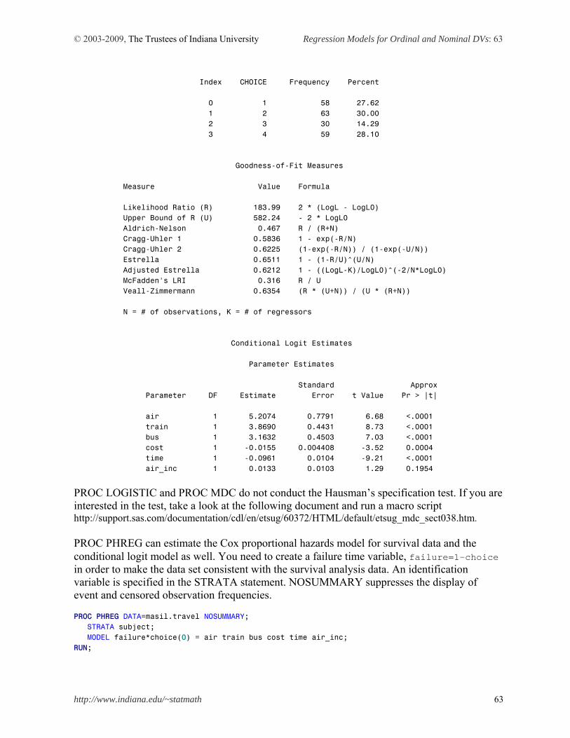
© 2003-2009, The Trustees of Indiana University Regression Models for Ordinal and Nominal DVs: 63
http://www.indiana.edu/~statmath 63
Index CHOICE Frequency Percent 0 1 58 27.62 1 2 63 30.00 2 3 30 14.29 3 4 59 28.10 Goodness-of-Fit Measures Measure Value Formula Likelihood Ratio (R) 183.99 2 * (LogL - LogL0) Upper Bound of R (U) 582.24 - 2 * LogL0 Aldrich-Nelson 0.467 R / (R+N) Cragg-Uhler 1 0.5836 1 - exp(-R/N) Cragg-Uhler 2 0.6225 (1-exp(-R/N)) / (1-exp(-U/N)) Estrella 0.6511 1 - (1-R/U)^(U/N) Adjusted Estrella 0.6212 1 - ((LogL-K)/LogL0)^(-2/N*LogL0) McFadden's LRI 0.316 R / U Veall-Zimmermann 0.6354 (R * (U+N)) / (U * (R+N)) N = # of observations, K = # of regressors Conditional Logit Estimates Parameter Estimates Standard Approx Parameter DF Estimate Error t Value Pr > |t| air 1 5.2074 0.7791 6.68 <.0001 train 1 3.8690 0.4431 8.73 <.0001 bus 1 3.1632 0.4503 7.03 <.0001 cost 1 -0.0155 0.004408 -3.52 0.0004 time 1 -0.0961 0.0104 -9.21 <.0001 air_inc 1 0.0133 0.0103 1.29 0.1954 PROC LOGISTIC and PROC MDC do not conduct the Hausman’s specification test. If you are interested in the test, take a look at the following document and run a macro script http://support.sas.com/documentation/cdl/en/etsug/60372/HTML/default/etsug_mdc_sect038.htm. PROC PHREG can estimate the Cox proportional hazards model for survival data and the conditional logit model as well. You need to create a failure time variable, failure=1–choice in order to make the data set consistent with the survival analysis data. An identification variable is specified in the STRATA statement. NOSUMMARY suppresses the display of event and censored observation frequencies. PROC PHREG DATA=masil.travel NOSUMMARY; STRATA subject; MODEL failure*choice(0) = air train bus cost time air_inc; RUN;
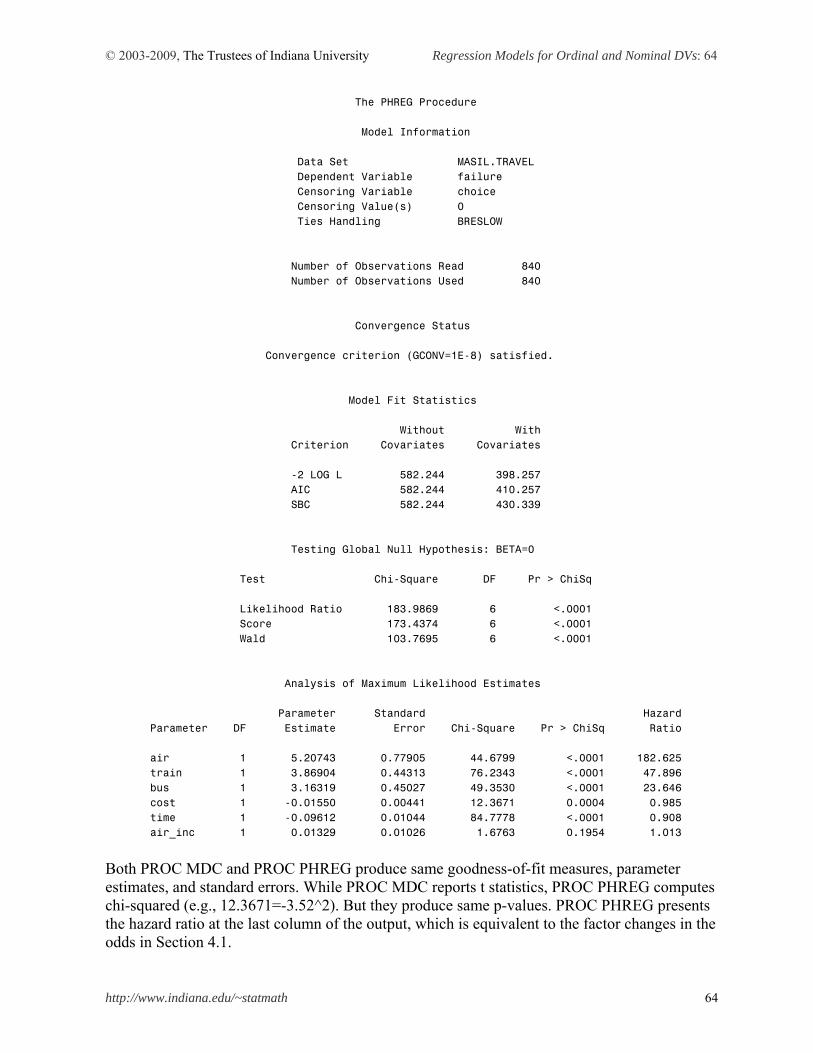
© 2003-2009, The Trustees of Indiana University Regression Models for Ordinal and Nominal DVs: 64
http://www.indiana.edu/~statmath 64
The PHREG Procedure Model Information Data Set MASIL.TRAVEL Dependent Variable failure Censoring Variable choice Censoring Value(s) 0 Ties Handling BRESLOW Number of Observations Read 840 Number of Observations Used 840 Convergence Status Convergence criterion (GCONV=1E-8) satisfied. Model Fit Statistics Without With Criterion Covariates Covariates -2 LOG L 582.244 398.257 AIC 582.244 410.257 SBC 582.244 430.339 Testing Global Null Hypothesis: BETA=0 Test Chi-Square DF Pr > ChiSq Likelihood Ratio 183.9869 6 <.0001 Score 173.4374 6 <.0001 Wald 103.7695 6 <.0001 Analysis of Maximum Likelihood Estimates Parameter Standard Hazard Parameter DF Estimate Error Chi-Square Pr > ChiSq Ratio air 1 5.20743 0.77905 44.6799 <.0001 182.625 train 1 3.86904 0.44313 76.2343 <.0001 47.896 bus 1 3.16319 0.45027 49.3530 <.0001 23.646 cost 1 -0.01550 0.00441 12.3671 0.0004 0.985 time 1 -0.09612 0.01044 84.7778 <.0001 0.908 air_inc 1 0.01329 0.01026 1.6763 0.1954 1.013 Both PROC MDC and PROC PHREG produce same goodness-of-fit measures, parameter estimates, and standard errors. While PROC MDC reports t statistics, PROC PHREG computes chi-squared (e.g., 12.3671=-3.52^2). But they produce same p-values. PROC PHREG presents the hazard ratio at the last column of the output, which is equivalent to the factor changes in the odds in Section 4.1.
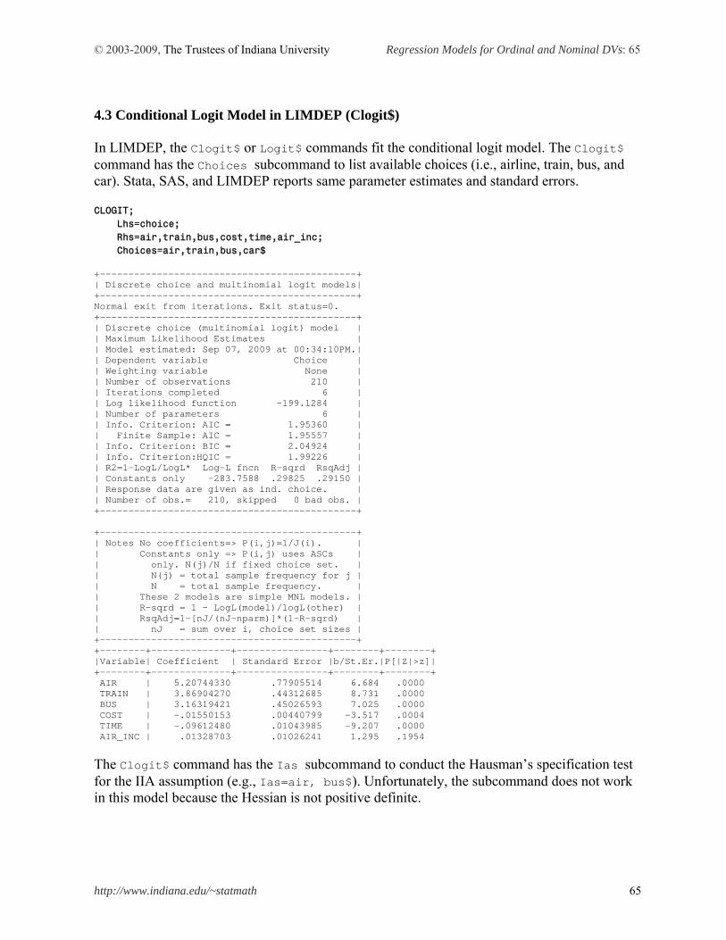
© 2003-2009, The Trustees of Indiana University Regression Models for Ordinal and Nominal DVs: 65
http://www.indiana.edu/~statmath 65
4.3 Conditional Logit Model in LIMDEP (Clogit$) In LIMDEP, the Clogit$ or Logit$ commands fit the conditional logit model. The Clogit$ command has the Choices subcommand to list available choices (i.e., airline, train, bus, and car). Stata, SAS, and LIMDEP reports same parameter estimates and standard errors. CLOGIT; Lhs=choice; Rhs=air,train,bus,cost,time,air_inc; Choices=air,train,bus,car$ +---------------------------------------------+ | Discrete choice and multinomial logit models| +---------------------------------------------+ Normal exit from iterations. Exit status=0. +---------------------------------------------+ | Discrete choice (multinomial logit) model | | Maximum Likelihood Estimates | | Model estimated: Sep 07, 2009 at 00:34:10PM.| | Dependent variable Choice | | Weighting variable None | | Number of observations 210 | | Iterations completed 6 | | Log likelihood function -199.1284 | | Number of parameters 6 | | Info. Criterion: AIC = 1.95360 | | Finite Sample: AIC = 1.95557 | | Info. Criterion: BIC = 2.04924 | | Info. Criterion:HQIC = 1.99226 | | R2=1-LogL/LogL* Log-L fncn R-sqrd RsqAdj | | Constants only -283.7588 .29825 .29150 | | Response data are given as ind. choice. | | Number of obs.= 210, skipped 0 bad obs. | +---------------------------------------------+ +---------------------------------------------+ | Notes No coefficients=> P(i,j)=1/J(i). | | Constants only => P(i,j) uses ASCs | | only. N(j)/N if fixed choice set. | | N(j) = total sample frequency for j | | N = total sample frequency. | | These 2 models are simple MNL models. | | R-sqrd = 1 - LogL(model)/logL(other) | | RsqAdj=1-[nJ/(nJ-nparm)]*(1-R-sqrd) | | nJ = sum over i, choice set sizes | +---------------------------------------------+ +--------+--------------+----------------+--------+--------+ |Variable| Coefficient | Standard Error |b/St.Er.|P[|Z|>z]| +--------+--------------+----------------+--------+--------+ AIR | 5.20744330 .77905514 6.684 .0000 TRAIN | 3.86904270 .44312685 8.731 .0000 BUS | 3.16319421 .45026593 7.025 .0000 COST | -.01550153 .00440799 -3.517 .0004 TIME | -.09612480 .01043985 -9.207 .0000 AIR_INC | .01328703 .01026241 1.295 .1954
The Clogit$ command has the Ias subcommand to conduct the Hausman’s specification test for the IIA assumption (e.g., Ias=air, bus$). Unfortunately, the subcommand does not work in this model because the Hessian is not positive definite.
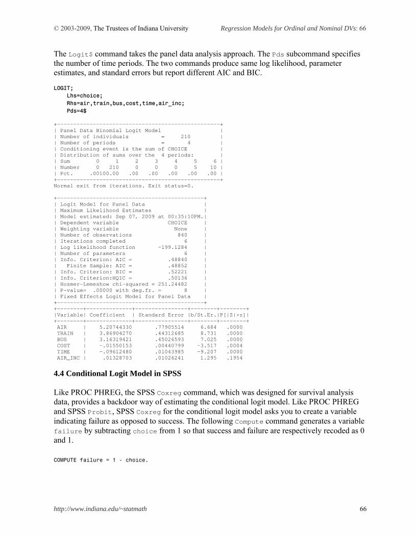
© 2003-2009, The Trustees of Indiana University Regression Models for Ordinal and Nominal DVs: 66
http://www.indiana.edu/~statmath 66
The Logit$ command takes the panel data analysis approach. The Pds subcommand specifies the number of time periods. The two commands produce same log likelihood, parameter estimates, and standard errors but report different AIC and BIC. LOGIT; Lhs=choice; Rhs=air,train,bus,cost,time,air_inc; Pds=4$ +--------------------------------------------------+ | Panel Data Binomial Logit Model | | Number of individuals = 210 | | Number of periods = 4 | | Conditioning event is the sum of CHOICE | | Distribution of sums over the 4 periods: | | Sum 0 1 2 3 4 5 6 | | Number 0 210 0 0 0 5 10 | | Pct. .00100.00 .00 .00 .00 .00 .00 | +--------------------------------------------------+ Normal exit from iterations. Exit status=0. +---------------------------------------------+ | Logit Model for Panel Data | | Maximum Likelihood Estimates | | Model estimated: Sep 07, 2009 at 00:35:10PM.| | Dependent variable CHOICE | | Weighting variable None | | Number of observations 840 | | Iterations completed 6 | | Log likelihood function -199.1284 | | Number of parameters 6 | | Info. Criterion: AIC = .48840 | | Finite Sample: AIC = .48852 | | Info. Criterion: BIC = .52221 | | Info. Criterion:HQIC = .50136 | | Hosmer-Lemeshow chi-squared = 251.24482 | | P-value= .00000 with deg.fr. = 8 | | Fixed Effects Logit Model for Panel Data | +---------------------------------------------+ +--------+--------------+----------------+--------+--------+ |Variable| Coefficient | Standard Error |b/St.Er.|P[|Z|>z]| +--------+--------------+----------------+--------+--------+ AIR | 5.20744330 .77905514 6.684 .0000 TRAIN | 3.86904270 .44312685 8.731 .0000 BUS | 3.16319421 .45026593 7.025 .0000 COST | -.01550153 .00440799 -3.517 .0004 TIME | -.09612480 .01043985 -9.207 .0000 AIR_INC | .01328703 .01026241 1.295 .1954
4.4 Conditional Logit Model in SPSS Like PROC PHREG, the SPSS Coxreg command, which was designed for survival analysis data, provides a backdoor way of estimating the conditional logit model. Like PROC PHREG and SPSS Probit, SPSS Coxreg for the conditional logit model asks you to create a variable indicating failure as opposed to success. The following Compute command generates a variable failure by subtracting choice from 1 so that success and failure are respectively recoded as 0 and 1.
COMPUTE failure = 1 - choice.
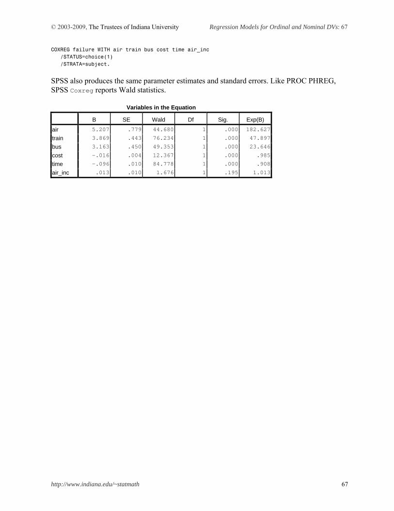
© 2003-2009, The Trustees of Indiana University Regression Models for Ordinal and Nominal DVs: 67
http://www.indiana.edu/~statmath 67
COXREG failure WITH air train bus cost time air_inc /STATUS=choice(1) /STRATA=subject. SPSS also produces the same parameter estimates and standard errors. Like PROC PHREG, SPSS Coxreg reports Wald statistics.
Variables in the Equation
B SE Wald Df Sig. Exp(B)
air 5.207 .779 44.680 1 .000 182.627
train 3.869 .443 76.234 1 .000 47.897
bus 3.163 .450 49.353 1 .000 23.646
cost -.016 .004 12.367 1 .000 .985
time -.096 .010 84.778 1 .000 .908
air_inc .013 .010 1.676 1 .195 1.013
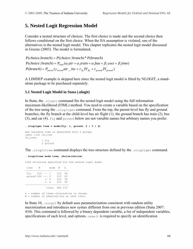
© 2003-2009, The Trustees of Indiana University Regression Models for Ordinal and Nominal DVs: 68
http://www.indiana.edu/~statmath 68
5. Nested Logit Regression Model Consider a nested structure of choices. The first choice is made and the second choice then follows conditional on the first choice. When the IIA assumption is violated, one of the alternatives is the nested logit model. This chapter replicates the nested logit model discussed in Greene (2003). The model is formulated,
)(*)|(),( branchPbranchchoicePbranchchoiceP
)cos()|( 21321 timetbustrainairPbranchchoiceP child
)_()( groundgroundflyflyincomeparent IVIVincairPbranchP A LIMDEP example is skipped here since the nested logit model is fitted by NLOGIT, a stand-alone package to be purchased separately. 5.1 Nested Logit Model in Stata (.nlogit) In Stata, the .nlogit command fits the nested logit model using the full information maximum-likelihood (FIML) method. You need to create a variable based on the specification of the tree using the .nlogitgen command. From the top, the parent-level has fly and ground branches; the fly branch at the child-level has air flight (1); the ground branch has train (2), bus (3), and car (4). fly and ground below are not variable names but arbitrary names you prefer. . nlogitgen tree = mode(fly: 1, ground: 2 | 3 | 4) new variable tree is generated with 2 groups label list lb_tree lb_tree: 1 fly 2 ground
The .nlogittree command displays the tree-structure defined by the .nlogitgen command. . nlogittree mode tree, choice(choice) tree structure specified for the nested logit model tree N mode N k ----------------------------- fly 210 --- 1 210 58 ground 630 --- 2 210 63 |- 3 210 30 +- 4 210 59 ----------------------------- total 840 210 k = number of times alternative is chosen N = number of observations at each level
In Stata 10, .nlogit by default uses parameterization consistent with random utility maximization and introduces new syntax different from one in previous edition (Stata 2007: 434). This command is followed by a binary dependent variable, a list of independent variables, specifications of each level, and options. case() is required to specify an identification
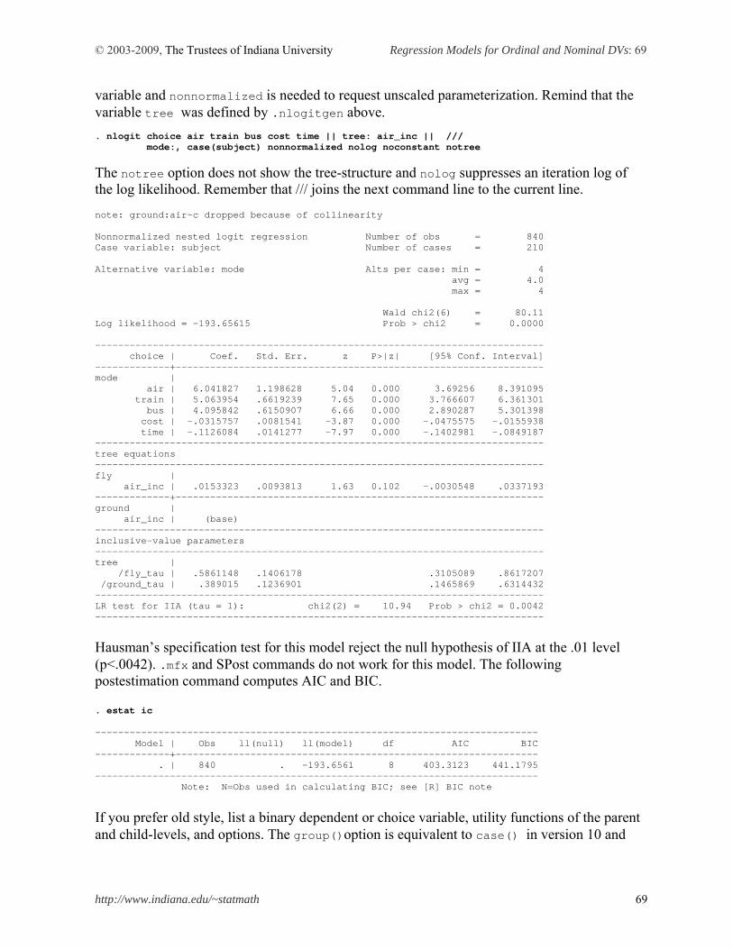
© 2003-2009, The Trustees of Indiana University Regression Models for Ordinal and Nominal DVs: 69
http://www.indiana.edu/~statmath 69
variable and nonnormalized is needed to request unscaled parameterization. Remind that the variable tree was defined by .nlogitgen above. . nlogit choice air train bus cost time || tree: air_inc || /// mode:, case(subject) nonnormalized nolog noconstant notree
The notree option does not show the tree-structure and nolog suppresses an iteration log of the log likelihood. Remember that /// joins the next command line to the current line. note: ground:air~c dropped because of collinearity Nonnormalized nested logit regression Number of obs = 840 Case variable: subject Number of cases = 210 Alternative variable: mode Alts per case: min = 4 avg = 4.0 max = 4 Wald chi2(6) = 80.11 Log likelihood = -193.65615 Prob > chi2 = 0.0000 ------------------------------------------------------------------------------ choice | Coef. Std. Err. z P>|z| [95% Conf. Interval] -------------+---------------------------------------------------------------- mode | air | 6.041827 1.198628 5.04 0.000 3.69256 8.391095 train | 5.063954 .6619239 7.65 0.000 3.766607 6.361301 bus | 4.095842 .6150907 6.66 0.000 2.890287 5.301398 cost | -.0315757 .0081541 -3.87 0.000 -.0475575 -.0155938 time | -.1126084 .0141277 -7.97 0.000 -.1402981 -.0849187 ------------------------------------------------------------------------------ tree equations ------------------------------------------------------------------------------ fly | air_inc | .0153323 .0093813 1.63 0.102 -.0030548 .0337193 -------------+---------------------------------------------------------------- ground | air_inc | (base) ------------------------------------------------------------------------------ inclusive-value parameters ------------------------------------------------------------------------------ tree | /fly_tau | .5861148 .1406178 .3105089 .8617207 /ground_tau | .389015 .1236901 .1465869 .6314432 ------------------------------------------------------------------------------ LR test for IIA (tau = 1): chi2(2) = 10.94 Prob > chi2 = 0.0042 ------------------------------------------------------------------------------
Hausman’s specification test for this model reject the null hypothesis of IIA at the .01 level (p<.0042). .mfx and SPost commands do not work for this model. The following postestimation command computes AIC and BIC. . estat ic ----------------------------------------------------------------------------- Model | Obs ll(null) ll(model) df AIC BIC -------------+--------------------------------------------------------------- . | 840 . -193.6561 8 403.3123 441.1795 ----------------------------------------------------------------------------- Note: N=Obs used in calculating BIC; see [R] BIC note
If you prefer old style, list a binary dependent or choice variable, utility functions of the parent and child-levels, and options. The group()option is equivalent to case() in version 10 and
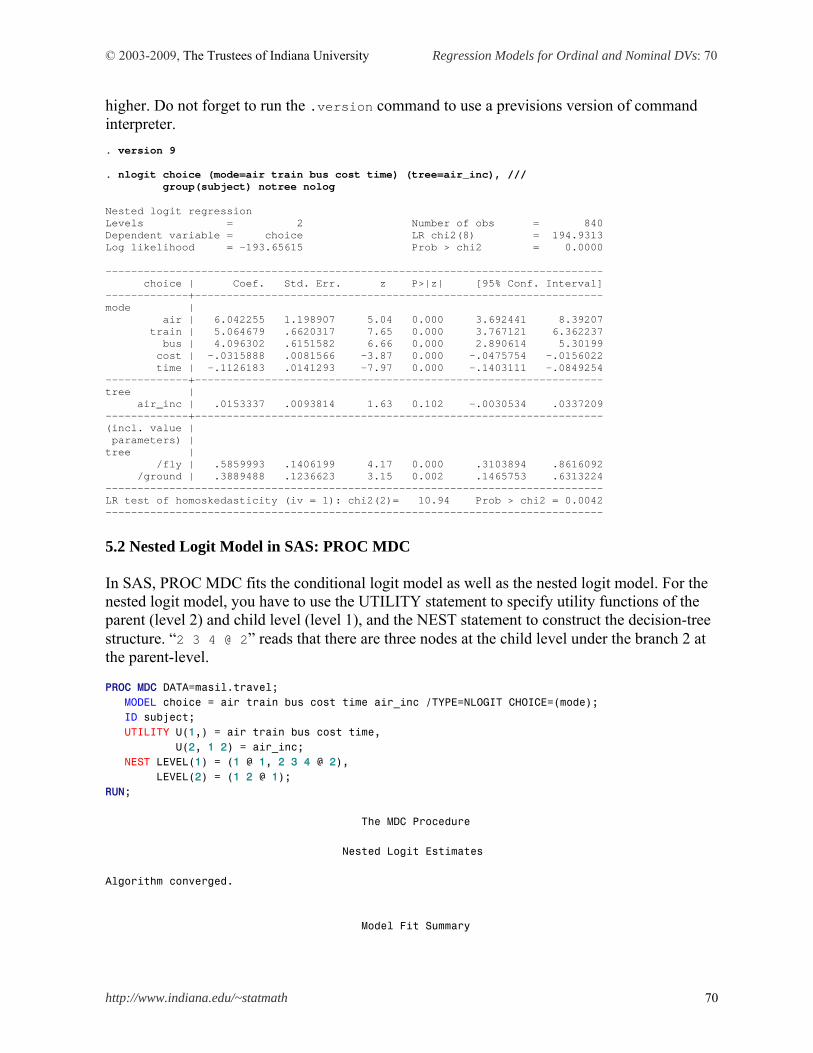
© 2003-2009, The Trustees of Indiana University Regression Models for Ordinal and Nominal DVs: 70
http://www.indiana.edu/~statmath 70
higher. Do not forget to run the .version command to use a previsions version of command interpreter. . version 9 . nlogit choice (mode=air train bus cost time) (tree=air_inc), /// group(subject) notree nolog Nested logit regression Levels = 2 Number of obs = 840 Dependent variable = choice LR chi2(8) = 194.9313 Log likelihood = -193.65615 Prob > chi2 = 0.0000 ------------------------------------------------------------------------------ choice | Coef. Std. Err. z P>|z| [95% Conf. Interval] -------------+---------------------------------------------------------------- mode | air | 6.042255 1.198907 5.04 0.000 3.692441 8.39207 train | 5.064679 .6620317 7.65 0.000 3.767121 6.362237 bus | 4.096302 .6151582 6.66 0.000 2.890614 5.30199 cost | -.0315888 .0081566 -3.87 0.000 -.0475754 -.0156022 time | -.1126183 .0141293 -7.97 0.000 -.1403111 -.0849254 -------------+---------------------------------------------------------------- tree | air_inc | .0153337 .0093814 1.63 0.102 -.0030534 .0337209 -------------+---------------------------------------------------------------- (incl. value | parameters) | tree | /fly | .5859993 .1406199 4.17 0.000 .3103894 .8616092 /ground | .3889488 .1236623 3.15 0.002 .1465753 .6313224 ------------------------------------------------------------------------------ LR test of homoskedasticity (iv = 1): chi2(2)= 10.94 Prob > chi2 = 0.0042 ------------------------------------------------------------------------------
5.2 Nested Logit Model in SAS: PROC MDC In SAS, PROC MDC fits the conditional logit model as well as the nested logit model. For the nested logit model, you have to use the UTILITY statement to specify utility functions of the parent (level 2) and child level (level 1), and the NEST statement to construct the decision-tree structure. “2 3 4 @ 2” reads that there are three nodes at the child level under the branch 2 at the parent-level. PROC MDC DATA=masil.travel; MODEL choice = air train bus cost time air_inc /TYPE=NLOGIT CHOICE=(mode); ID subject; UTILITY U(1,) = air train bus cost time, U(2, 1 2) = air_inc; NEST LEVEL(1) = (1 @ 1, 2 3 4 @ 2), LEVEL(2) = (1 2 @ 1); RUN; The MDC Procedure Nested Logit Estimates Algorithm converged. Model Fit Summary
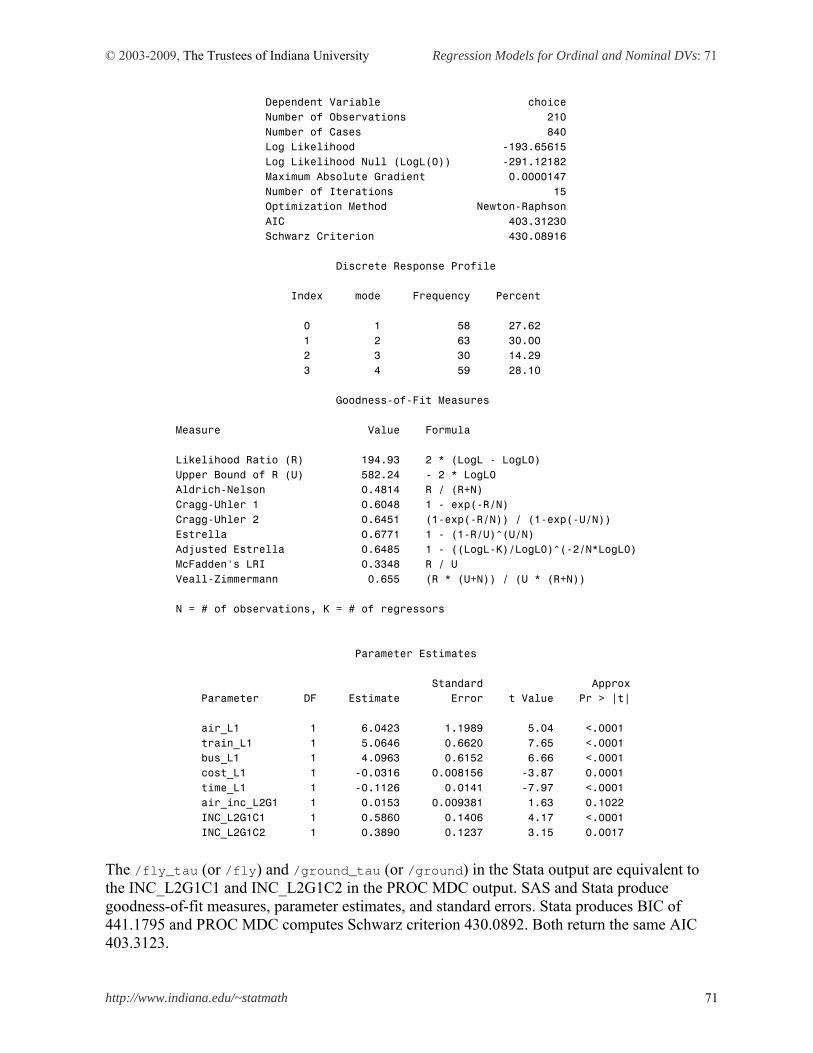
© 2003-2009, The Trustees of Indiana University Regression Models for Ordinal and Nominal DVs: 71
http://www.indiana.edu/~statmath 71
Dependent Variable choice Number of Observations 210 Number of Cases 840 Log Likelihood -193.65615 Log Likelihood Null (LogL(0)) -291.12182 Maximum Absolute Gradient 0.0000147 Number of Iterations 15 Optimization Method Newton-Raphson AIC 403.31230 Schwarz Criterion 430.08916 Discrete Response Profile Index mode Frequency Percent 0 1 58 27.62 1 2 63 30.00 2 3 30 14.29 3 4 59 28.10 Goodness-of-Fit Measures Measure Value Formula Likelihood Ratio (R) 194.93 2 * (LogL - LogL0) Upper Bound of R (U) 582.24 - 2 * LogL0 Aldrich-Nelson 0.4814 R / (R+N) Cragg-Uhler 1 0.6048 1 - exp(-R/N) Cragg-Uhler 2 0.6451 (1-exp(-R/N)) / (1-exp(-U/N)) Estrella 0.6771 1 - (1-R/U)^(U/N) Adjusted Estrella 0.6485 1 - ((LogL-K)/LogL0)^(-2/N*LogL0) McFadden's LRI 0.3348 R / U Veall-Zimmermann 0.655 (R * (U+N)) / (U * (R+N)) N = # of observations, K = # of regressors Parameter Estimates Standard Approx Parameter DF Estimate Error t Value Pr > |t| air_L1 1 6.0423 1.1989 5.04 <.0001 train_L1 1 5.0646 0.6620 7.65 <.0001 bus_L1 1 4.0963 0.6152 6.66 <.0001 cost_L1 1 -0.0316 0.008156 -3.87 0.0001 time_L1 1 -0.1126 0.0141 -7.97 <.0001 air_inc_L2G1 1 0.0153 0.009381 1.63 0.1022 INC_L2G1C1 1 0.5860 0.1406 4.17 <.0001 INC_L2G1C2 1 0.3890 0.1237 3.15 0.0017 The /fly_tau (or /fly) and /ground_tau (or /ground) in the Stata output are equivalent to the INC_L2G1C1 and INC_L2G1C2 in the PROC MDC output. SAS and Stata produce goodness-of-fit measures, parameter estimates, and standard errors. Stata produces BIC of 441.1795 and PROC MDC computes Schwarz criterion 430.0892. Both return the same AIC 403.3123.
© 2003-2009, The Trustees of Indiana University Regression Models for Ordinal and Nominal DVs: 72
http://www.indiana.edu/~statmath 72
6. Conclusion The regression models discussed so far are of categorical dependent variables (binary, ordinal, and nominal responses). An appropriate regression model is determined largely by the measurement level of a categorical dependent variable of interest. The level of measurement should be, however, considered in conjunction with your theory and research questions (Long 1997). You must also examine the data generation process (DGP) of a dependent variable to understand its “behavior.” Experienced researchers pay special attention to censoring, truncation, sample selection, and other particular patterns of the DGP although these limited dependent variable issues are not addressed here. Generally speaking, if your dependent variable is a binary variable, you may use the binary logit or probit regression model. For ordinal responses, try to fit either ordered logit or probit regression model. If you have a nominal response variable, investigate the DGP carefully and then choose one of the multinomial logit, conditional logit, and nested logit models. In order to use the conditional logit and nested logit, you need to reshape the data set in advance. You should check key assumptions of a model when fitting the model. Examples are the parallel regression assumption in ordered logit and probit models and the independence of irrelevant alternatives (IIA) assumption in the multinomial logit model. You may respectively conduct the Brant test and Hausman test for these assumptions. If an assumption of an ordered or nominal response model is violated, find alternative models or think carefully if a dependent variable can be explored in a binary response model by dichotomizing the variable. Since logit and probit models are nonlinear, their parameter estimates are difficult to interpret intuitively. The situation becomes even worse in generalized ordered logit and multinomial logit models, where many parameter estimates and related statistics are produced. Consequently, researchers need to spend more time and effort interpreting the results substantively. Simply reporting parameter estimates and goodness-of-fit statistics is not sufficient. J. Scott Long (1997) and Long and Freese (2003) provide good examples of meaningful interpretations using predicted probabilities, factor changes in odds, and marginal effects (discrete changes) of predicted probabilities. It is highly recommended to visualize marginal effects and discrete changes using a plot of predicted probabilities. In general, logit and probit models require larger N than do linear regression models. Like the Bayesian estimation method, the maximum likelihood estimation method depends on data. You need to check if you have sufficient valid observations especially when your data contain many missing values. Scott Long’s rule of thumb says 500 observations and at least additional 10 per independent variable are required in ML estimation. If you have small N, DO NOT include a large number of independent variables. This is the so called “small N and large parameter” problem; you may not be able to reach convergence in estimation (you are just torturing SAS or Stata to get nothing) and/or may not get reliable results with desirable asymptotic ML properties. What if 10 parameters are estimated on the basis of 50 observations? By contrast, an extremely large N, say millions to estimate only two parameters, is not always a virtue since it absurdly boosts the statistical power of a test without adding new information. Even a tiny
© 2003-2009, The Trustees of Indiana University Regression Models for Ordinal and Nominal DVs: 73
http://www.indiana.edu/~statmath 73
effect, which should have been negligible in a normal situation, may be mistakenly reported as statistically significant. Regarding statistical software packages, I would recommend the SAS LOGISTIC, QLIM, and MDC procedures of SAS/ETS (see Table 2.1 and 3.1). SAS also has PROC GENMOD and PROC PROBIT, but PROC LOGISTIC and PROC QLIM appear to be best for binary and ordinal response models, and PROC MDC is good for nominal dependent variable models. ODS is another advantage of using SAS. I also strongly recommend Stata since it provides handy ways to fit various models and also can be assisted by SPost, which has various useful commands such as .fitstat, .prchange, .listcoef, .prtab, and .prgen. I encourage SAS Institute to develop additional statements similar to, in particular, .prchange and .prgen. LIMDEP supports various regression models for categorical dependent variables addressed in Greene (2003) but does not seem as user-friendly and stable as SAS and Stata. However, LIMDEP computes direct and indirect effects in the recursive bivariate probit model and helps researchers interpret the result in more detail. You may benefits from R’s object-oriented programming concept and analyze data flexibly in your own way. SPSS is least recommended mainly due to its limited support for categorical dependent variable models and messy syntax and output. If you are interested in logit and probit models for binary outcome variables, see Park, Hun Myoung. 2009. Regression Models for Binary Dependent Variables Using Stata, SAS, R, LIMDEP, and SPSS. Working Paper. The University Information Technology Services (UITS) Center for Statistical and Mathematical Computing, Indiana University.” http://www.indiana.edu/~statmath/stat/all/cdvm/index.html
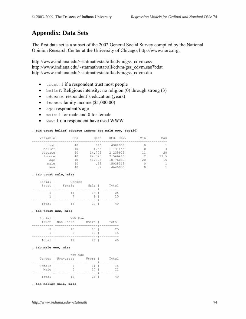
© 2003-2009, The Trustees of Indiana University Regression Models for Ordinal and Nominal DVs: 74
http://www.indiana.edu/~statmath 74
Appendix: Data Sets The first data set is a subset of the 2002 General Social Survey compiled by the National Opinion Research Center at the University of Chicago, http://www.norc.org. http://www.indiana.edu/~statmath/stat/all/cdvm/gss_cdvm.csv http://www.indiana.edu/~statmath/stat/all/cdvm/gss_cdvm.sas7bdat http://www.indiana.edu/~statmath/stat/all/cdvm/gss_cdvm.dta
trust: 1 if a respondent trust most people belief: Religious intensity: no religion (0) through strong (3) educate: respondent’s education (years) income: family income ($1,000.00) age: respondent’s age male: 1 for male and 0 for female www: 1 if a respondent have used WWW
. sum trust belief educate income age male www, sep(20) Variable | Obs Mean Std. Dev. Min Max -------------+-------------------------------------------------------- trust | 40 .375 .4902903 0 1 belief | 40 1.55 1.131144 0 3 educate | 40 14.775 2.235925 11 20 income | 40 24.325 7.566415 2 27.5 age | 40 41.825 10.76053 20 65 male | 40 .55 .5038315 0 1 www | 40 .7 .4640955 0 1 . tab trust male, miss Social | Gender Trust | Female Male | Total -----------+----------------------+---------- 0 | 11 14 | 25 1 | 7 8 | 15 -----------+----------------------+---------- Total | 18 22 | 40 . tab trust www, miss Social | WWW Use Trust | Non-users Users | Total -----------+----------------------+---------- 0 | 10 15 | 25 1 | 2 13 | 15 -----------+----------------------+---------- Total | 12 28 | 40 . tab male www, miss | WWW Use Gender | Non-users Users | Total -----------+----------------------+---------- Female | 7 11 | 18 Male | 5 17 | 22 -----------+----------------------+---------- Total | 12 28 | 40 . tab belief male, miss
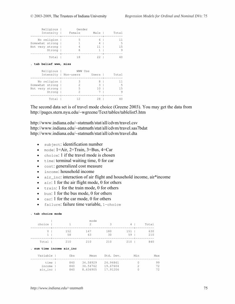
© 2003-2009, The Trustees of Indiana University Regression Models for Ordinal and Nominal DVs: 75
http://www.indiana.edu/~statmath 75
Religious | Gender Intensity | Female Male | Total ----------------+----------------------+---------- No religion | 5 6 | 11 Somewhat strong | 1 4 | 5 Not very strong | 4 11 | 15 Strong | 8 1 | 9 ----------------+----------------------+---------- Total | 18 22 | 40 . tab belief www, miss Religious | WWW Use Intensity | Non-users Users | Total ----------------+----------------------+---------- No religion | 3 8 | 11 Somewhat strong | 2 3 | 5 Not very strong | 5 10 | 15 Strong | 2 7 | 9 ----------------+----------------------+---------- Total | 12 28 | 40
The second data set is of travel mode choice (Greene 2003). You may get the data from http://pages.stern.nyu.edu/~wgreene/Text/tables/tablelist5.htm http://www.indiana.edu/~statmath/stat/all/cdvm/travel.csv http://www.indiana.edu/~statmath/stat/all/cdvm/travel.sas7bdat http://www.indiana.edu/~statmath/stat/all/cdvm/travel.dta
subject: identification number mode: 1=Air, 2=Train, 3=Bus, 4=Car choice: 1 if the travel mode is chosen time: terminal waiting time, 0 for car cost: generalized cost measure income: household income air_inc: interaction of air flight and household income, air*income air: 1 for the air flight mode, 0 for others train: 1 for the train mode, 0 for others bus: 1 for the bus mode, 0 for others car: 1 for the car mode, 0 for others failure: failure time variable, 1-choice
. tab choice mode | mode choice | 1 2 3 4 | Total -----------+--------------------------------------------+---------- 0 | 152 147 180 151 | 630 1 | 58 63 30 59 | 210 -----------+--------------------------------------------+---------- Total | 210 210 210 210 | 840 . sum time income air_inc Variable | Obs Mean Std. Dev. Min Max -------------+-------------------------------------------------------- time | 840 34.58929 24.94861 0 99 income | 840 34.54762 19.67604 2 72 air_inc | 840 8.636905 17.91206 0 72
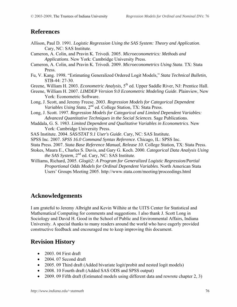
© 2003-2009, The Trustees of Indiana University Regression Models for Ordinal and Nominal DVs: 76
http://www.indiana.edu/~statmath 76
References Allison, Paul D. 1991. Logistic Regression Using the SAS System: Theory and Application.
Cary, NC: SAS Institute. Cameron, A. Colin, and Pravin K. Trivedi. 2005. Microeconometrics: Methods and
Applications. New York: Cambridge University Press. Cameron, A. Colin, and Pravin K. Trivedi. 2009. Microeconometrics Using Stata. TX: Stata
Press. Fu, V. Kang. 1998. “Estimating Generalized Ordered Logit Models,” Stata Technical Bulletin,
STB-44: 27-30. Greene, William H. 2003. Econometric Analysis, 5th ed. Upper Saddle River, NJ: Prentice Hall. Greene, William H. 2007. LIMDEP Version 9.0 Econometric Modeling Guide. Plainview, New
York: Econometric Software. Long, J. Scott, and Jeremy Freese. 2003. Regression Models for Categorical Dependent
Variables Using Stata, 2nd ed. College Station, TX: Stata Press. Long, J. Scott. 1997. Regression Models for Categorical and Limited Dependent Variables:
Advanced Quantitative Techniques in the Social Sciences. Sage Publications. Maddala, G. S. 1983. Limited Dependent and Qualitative Variables in Econometrics. New
York: Cambridge University Press. SAS Institute. 2004. SAS/STAT 9.1 User's Guide. Cary, NC: SAS Institute. SPSS Inc. 2007. SPSS 16.0 Command Syntax Reference. Chicago, IL: SPSS Inc. Stata Press. 2007. Stata Base Reference Manual, Release 10. College Station, TX: Stata Press. Stokes, Maura E., Charles S. Davis, and Gary G. Koch. 2000. Categorical Data Analysis Using
the SAS System, 2nd ed. Cary, NC: SAS Institute. Williams, Richard, 2005. Glogit2: A Program for Generalized Logistic Regression/Partial
Proportional Odds Models for Ordinal Dependent Variables. North American Stata Users’ Groups Meeting 2005. http://www.stata.com/meeting/proceedings.html
Acknowledgements I am grateful to Jeremy Albright and Kevin Wilhite at the UITS Center for Statistical and Mathematical Computing for comments and suggestions. I also thank J. Scott Long in Sociology and David H. Good in the School of Public and Environmental Affairs, Indiana University. A special thanks to many readers around the world who have eagerly provided constructive feedback and encouraged me to keep improving this document. Revision History
2003. 04 First draft 2004. 07 Second draft 2005. 09 Third draft (Added bivariate logit/probit and nested logit models) 2008. 10 Fourth draft (Added SAS ODS and SPSS output) 2009. 09 Fifth draft (Estimated models using different data and rewrote chapter 2, 3)


![6 Multilevel Models for Ordinal and Nominal Variables · [52] described an extension of the multilevel ordinal logistic regression model to allow for non-proportional odds for a set](https://static.fdocuments.us/doc/165x107/5e8abb285fb7bf31e54d874f/6-multilevel-models-for-ordinal-and-nominal-variables-52-described-an-extension.jpg)