Regression Models for Binary

Time Series with Gaps

Bernhard Klingenberg

Department of Mathematics and Statistics

Williams College, Williamstown, MA 01267

email: bklingen@williams.edu

November 15, 2007

Abstract

Time series of discrete random variables present unique statistical challenges due to

serial correlation and uneven sampling intervals. While regression models for a series of

counts are well developed, only few methods are discussed for the analysis of moderate

to long (e.g. from 20 to 152 observations) binary or binomial time series. This article

suggests generalized linear mixed models with autocorrelated random effects for a

parameter driven approach to such series. We use a Monte Carlo EM algorithm to

jointly obtain maximum likelihood estimates of regression parameters and variance

components. The likelihood approach, although computationally extensive, allows

estimation of marginal joint probabilities of two or more serial events. These are

crucial in checking the goodness of fit, whether the model adequately captures the

serial correlation and for predicting future responses. The model is flexible enough to

allow for missing observations or unequally spaced time intervals. We illustrate our

approach and model assessment tools with an analysis of the series of winners in the

traditional boat race between the universities of Oxford and Cambridge, re-evaluating

a long-held belief about the effect of the weight of the crew on the odds of winning.

We also show how our methods are useful in modeling trends based on the General

Social Survey database.

KEY WORDS: Autocorrelated random effects; Correlated binary data; Discrete time

series; Generalized linear mixed models; Logistic regression

1

1 Introduction

Generalized Linear Mixed models (GLMMs) are now a well established class to model

correlated discrete data from clustered or longitudinal studies. In general, however,

such studies are only concerned with a few repeated measurements and often assume

exchangeable correlation structures where the time lag between observations is not

accounted for. In this article we develop GLMMs for much longer (e.g. 152 obser-

vations) and unequally spaced time series of discrete observations with a decaying

correlation pattern.

Let Yt be a discrete response at time t, t = 1, . . . , T , observed together with a

vector of covariates denoted by xt, whose effect is described by a parameter vector β.

A basic generalized linear model (GLM) models the mean of Yt through a link function

l(.) depending on a linear predictor x′tβ, but assumes independent observations. To

accommodate time series, extensions of basic GLMs are characterized by the way serial

correlation is built into them. In marginal models, a (working) correlation is specified

directly while in transitional, observation-driven or Markov chain models correlation is

introduced by including functions of past responses in the linear predictor. The mean

is then modeled conditional on these past responses. In contrast, random effects or

parameter-driven models such as the GLMM induce correlation by including random

effects and model the conditional mean of Yt given these random effects.

The way serial correlation is built into a model also determines the type of infer-

ence. Typically, marginal models for discrete time series are fit by a quasi-likelihood

approach using generalized estimating equations (GEE). Estimation in transitional

models is based on a conditional or partial likelihood and inference in random effects

models often relies on a computationally intensive full likelihood approach. This is

exemplified by the analysis of a data set on 168 monthly counts of cases of poliomyeli-

tis in the United States. All three major modeling approaches were used to analyze

1

this time series of counts, starting with Zeger (1988), who used GEE methodology

to fit a marginal Poisson model. Li (1994), Fahrmeir and Tutz (2001) and Benjamin

et al. (2003) proposed transitional models based on a conditional Poisson or negative

binomial assumption. Chan and Ledolter (1995) developed GLMMs with AR(1) ran-

dom effects (see also Kuk and Cheng, 1999). Davis et al. (2000) discussed testing and

estimation in these parameter driven models further and Davis and Rodriguez-Yam

(2005) fitted state space models (Durbin and Koopman, 2000) to the polio data, a

model class closely related to GLMMs. Jung et al. (2006) compared many of these

models and proposed efficient estimation routines. Chen and Ibrahim (2000) consid-

ered a Bayesian analysis of the basic model by Zeger (1988), focusing on constructing

informative priors from historical data and evaluating the predictive ability of com-

peting models. Hay and Pettitt (2001) gave a fully Bayesian treatment for series of

counts, using AR(1) and alternative distributional assumptions for the random effects.

Regression models for binary time series received less attention and are confined

to methods developed for a small number of repeated observations in a longitudinal

context, see Diggle et al. (2002) or Fitzmaurice et al. (2004) for a detailed discussion.

Kedem and Fokianos (2002) and Fokianos and Kedem (2004) discuss transitional

models for long binary time series, using a partial likelihood approach. However, two

drawbacks of these models are that unequally spaced time series cannot be routinely

handled and interpretation of regression parameters depends on and changes with the

number of past responses conditioned on. MacDonald and Zucchini (1997) describe

Hidden Markov models which assume a discrete-state Markov chain for the evolution of

random effects over time. An advantage of these models over a GLMM or state space

approach is that maximum likelihood estimation is relatively straightforward, but

methods for unequally spaced data are also not available. In the Bayesian literature,

Sun et al. (1999, 2000) explore models with autoregressive random effects for discrete

time series. One of their results applied to Poisson or binary data states that the

2

posterior might be improper when Yt = 0 in the Poisson case and cannot be proper in

the binary case when common improper priors on the autoregressive random effects

are used. Hence the binary time series considered in this article can only be fit by their

methods when a proper prior on the random effects is used. Czado (2000) and Liu

(2001) also describe Bayesian models for binary time series, based on the multivariate

probit model developed in Chib and Greenberg (1998). In a spatial context, Pettitt et

al. (2002) model the latent variable that leads to the probit model via tresholding by a

Gaussian conditional autoregressive process, maintaining computational simplicity for

simulating from the posterior via MCMC. They consider irregularly spaced observation

sites and allow for covariates in the mean of the latent variable.

Although all approaches above incorporate the serial dependence in one way or

another, (i) unequally spaced time intervals or missing observations, (ii) the appro-

priateness of the assumed serial correlation structure, (iii) the fit of the model and

(iv) forecasting future observations are usually not discussed in a single framework.

This is natural for longitudinal data and a marginal approach, where the correlation is

considered a nuisance and scientific interest focuses on marginal parameters, which are

robust to misspecification of the correlation. Similarly, for time series, the main focus

is on describing its trend, but emphasis must also be on an appropriate model for the

serial correlation and its interpretation. The contribution of this paper is to address

these goals together with points (i) − (iv). We propose GLMMs with autoregressive

random effects as a general framework of modeling discrete time series. The model and

its implied higher order marginal properties, useful for model checking and forecasting,

are derived in Section 2. Algorithmic details of obtaining maximum likelihood esti-

mates, incorporating unequally spaced observations, are given in Section 3, together

with a simulation study. In Section 4, time series from two different backgrounds are

analyzed and procedures for model checking and forecasting are developed. Section 5

concludes with a summary and brief discussion.

3

2 GLMMs with autoregressive random effects

In this section, we allow for multiple observations Yit, i = 1, . . . , k at a common

time point t, although later we will focus on the case k = 1, but see the example

in Section 4.2. To incorporate serial dependence in a discrete time series model,

we initially follow the parameter driven approach of Chan and Ledolter (1995) by

including a latent autoregressive process {ut} in the linear predictor of a GLMM (see

also Diggle et al. 2002, Chpt. 11.2). Conditional on this latent process, observations

Y t = (Y1t, . . . , Ykt) at time points t = 1, . . . , T (not necessarily equally spaced) are

assumed independent with distributions f(yt|ut) =∏k

i=1 f(yit|ut) in the exponential

family. With inverse link function l−1(.), the model for the conditional mean has form

µit = E[Yit|ut] = l−1(x′itβ + ut),

and we establish a link between successive means through ut+1 = ρdtut + εt, t =

1, . . . , T − 1, where ρ is an autocorrelation parameter, dt is the time lag between ob-

serving Yit and Yi(t+1), εt ind. N(0, σ2[1−ρ2dt ]) and u1 ∼ N(0, σ2). The AR(1) process

{ut}, parameterized such that Var(ut) = σ2 for all t and Corr(ut, ut′) = ρ∑t′

k=t dk ,

describes unobserved factors that induce heterogeneity and serial correlation. In the

following, we will focus on GLMMs with AR(1) random effects for a single binary time

series, but similar results can be derived for binomial, Poisson or negative binomial

outcomes. Further, we will consider the logit link, as it is the natural parameter to

model when it comes to interpreting effects and correlation over time.

2.1 Binary time series

Conditional on time specific random effects {ut}Tt=1, let {Yt}T

t=1 be independent binary

random variables with conditional success probabilities πt(ut) = P (Yt = 1|ut). Using

a logit link, a GLMM with AR(1) random effects (AR-GLMMs) allowing for serially

4

correlated log-odds is given by

logit[πt(ut)] = x′tβ + ut, ut+1 = ρdtut + εt. (1)

Marginally, observations {Yt} have means E[Yt] = πMt = E[πt(ut)] and variances

Var[Yt] = πMt (1 − πM

t ). Because Cov[Yt, Yt+h] = Cov [πt(ut), πt+h(ut+h)], correlated

random effects induce a marginal serial correlation among observations. For binary

time series, especially those with gaps, it is more intuitive to measure this association

with the Lorelogram (Heagerty and Zeger, 1998), defined as the log odds ratio between

two binary observations h time units apart,

θt(h) = log

[P (Yt = 1, Yt+h = 1)× P (Yt = 0, Yt+h = 0)

P (Yt = 1, Yt+h = 0)× P (Yt = 0, Yt+h = 1)

]. (2)

Evaluating these marginal expressions is important for model interpretation and

for assessing the appropriateness of the assumed correlation structure, but no closed

forms exist. However, they can be approximated through Monte Carlo integration or,

analytically, by exploiting connections between (conditional) logit and probit links.

For any subsequence of p responses {Ytk}pk=1 (not necessarily consecutive) with out-

comes a1, . . . , ap ∈ {0, 1}, rewrite the linear predictor in (1) as ηtk = x′tkβ + σztk ,

where σ is interpreted as a regression parameter for the standardized random effect

ztk . Conditional on z = (zt1 , . . . , ztp), we wish to determine coefficients c1, . . . , cp such

that the joint p−dimensional probabilities are approximately equal under the logit

and probit models, i.e.,

p∏

k=1

exp(akηtk)/[1 + exp(ηtk)] ≈p∏

k=1

Φ[(−1)1−akηtk/ck

], (3)

where Φ denotes the standard normal cdf. Note that for (ηt1 , . . . , ηtp) = 0, both

the left and right hand side in (3) are, in fact, equal to 1/2p for all possible ak’s.

One way to determine c1 through cp through a first order approximation is to equate

the gradients, evaluated at (ηt1 , . . . , ηtp) = 0. It is straightforward to show that this

5

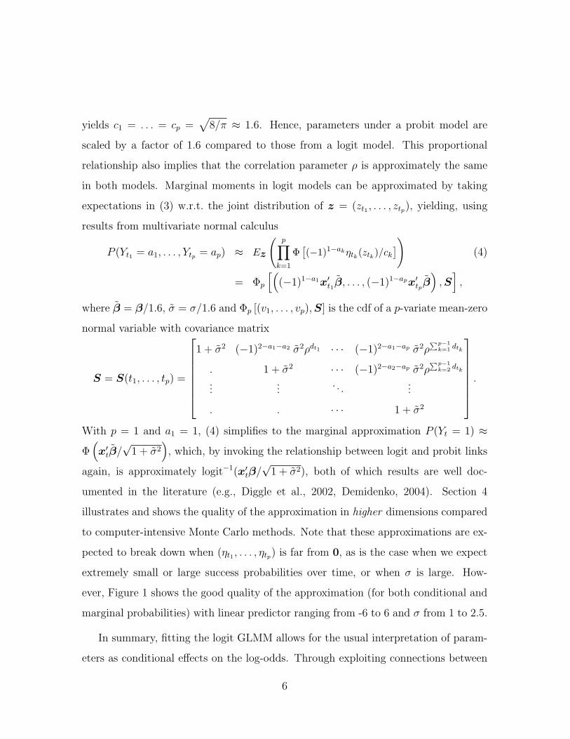
yields c1 = . . . = cp =√

8/π ≈ 1.6. Hence, parameters under a probit model are

scaled by a factor of 1.6 compared to those from a logit model. This proportional

relationship also implies that the correlation parameter ρ is approximately the same

in both models. Marginal moments in logit models can be approximated by taking

expectations in (3) w.r.t. the joint distribution of z = (zt1 , . . . , ztp), yielding, using

results from multivariate normal calculus

P (Yt1 = a1, . . . , Ytp = ap) ≈ Ez

(p∏

k=1

Φ[(−1)1−akηtk(ztk)/ck

])

(4)

= Φp

[((−1)1−a1x′t1β, . . . , (−1)1−apx′tpβ

),S

],

where β = β/1.6, σ = σ/1.6 and Φp [(v1, . . . , vp),S] is the cdf of a p-variate mean-zero

normal variable with covariance matrix

S = S(t1, . . . , tp) =

1 + σ2 (−1)2−a1−a2 σ2ρdt1 · · · (−1)2−a1−ap σ2ρ∑p−1

k=1 dtk

. 1 + σ2 · · · (−1)2−a2−ap σ2ρ∑p−1

k=2 dtk

......

. . ....

. . · · · 1 + σ2

.

With p = 1 and a1 = 1, (4) simplifies to the marginal approximation P (Yt = 1) ≈Φ

(x′tβ/

√1 + σ2

), which, by invoking the relationship between logit and probit links

again, is approximately logit−1(x′tβ/√

1 + σ2), both of which results are well doc-

umented in the literature (e.g., Diggle et al., 2002, Demidenko, 2004). Section 4

illustrates and shows the quality of the approximation in higher dimensions compared

to computer-intensive Monte Carlo methods. Note that these approximations are ex-

pected to break down when (ηt1 , . . . , ηtp) is far from 0, as is the case when we expect

extremely small or large success probabilities over time, or when σ is large. How-

ever, Figure 1 shows the good quality of the approximation (for both conditional and

marginal probabilities) with linear predictor ranging from -6 to 6 and σ from 1 to 2.5.

In summary, fitting the logit GLMM allows for the usual interpretation of param-

eters as conditional effects on the log-odds. Through exploiting connections between

6

logit and probit links, we can give accurate closed form approximations for marginal

probabilities, odds and correlations, useful for model interpretation, checking and fore-

casting. This is in the spirit of Lee and Nelder (2004), who regard the conditional

model as the fundamental formulation from which marginal predictions are derived.

3 Maximum likelihood fitting of AR-GLMMs

Maximum likelihood estimation of β and variance components ψ = (σ, ρ) in AR-

GLMMs is a challenging task, because it involves integrals with dimension equal to

T . Let y = (y1, . . . , yT ) and u = (u1, . . . , uT ) be the vector of all observations and

random effects, with densities f(y|u; β) =∏T

t=1 f(yt|ut; β) and g(u; ψ), respectively.

The likelihood function L(β, ψ; y) is given by the marginal density of y, obtained by

integrating over the AR(1) random effects,

L(β,ψ; y) =

∫f(y1|u1; β)g(u1; ψ)

T∏t=2

f(yt|ut; β)g(ut|ut−1; ψ)du. (5)

This integral has no closed-form solution and numerical procedures are necessary to

calculate and maximize it. Let β(k−1) and ψ(k−1) denote current (at the end of iteration

k− 1) estimates of parameter vectors β and ψ. With the Monte Carlo EM (MCEM)

algorithm, (5) is indirectly maximized by maximizing the Monte Carlo approximation

Qm(β,ψ|β(k−1), ψ(k−1)) =1

m

m∑j=1

log f(y|u(j); β) +1

m

m∑j=1

log g(u(j); ψ). (6)

of the so-called Q function (Wei and Tanner, 1990). This approximation uses a sample

u(1), . . . , u(m) from the conditional distribution h(u|y; β(k−1),ψ(k−1)) of the random

effects given the observed data, which is described in Appendix A.

Let Q1m and Q2

m be the first and second sum in (6). Maximizing Q1m with respect

to β is equivalent to fitting an augmented GLM with known offsets u(j). We duplicate

7

the original data set m times and attach the known offset u(j) to the jth replicate.

The log-likelihood equations for this augmented GLM are proportional to Q1m and

maximization can follow along the lines of well known, iterative Newton-Raphson or

Fisher scoring algorithms. Maximizing Q2m with respect to ψ is equivalent to finding

MLEs of σ and ρ for the sample of u(1), . . . , u(m), pretending they are independent.

With unequally spaced time series, this is more involved. For fixed ρ, maximizing Q2m

with respect to σ is possible in closed form, but iteration has to be used for finding the

MLE of ρ, except in the case of equally spaced time series. Appendix B gives details.

3.1 Convergence criteria

Due to the stochastic nature of the algorithm, parameter estimates of two successive it-

erations can be close together just by chance, although convergence is not yet achieved.

To reduce the risk of stopping prematurely we declare convergence if the maximum

relative change in parameter estimates λ(k) = (β(k)′,ψ(k)′)′ is less than some ε1, i.e.,

maxi

(|λ(k)

i − λ(k−1)i |/|λ(k−1)

i |)≤ ε1 for c (e.g. 4) consecutive times. An exception to

this rule occurs when the estimated standard error of a parameter is substantially

larger than the change from one iteration to the next (Booth and Hobert, 1999). Es-

timated standard errors for the MLE λ are obtained by approximating the observed

information matrix I(λ) = −∂2 log L(λ; y)/∂λ∂λ′|λ=

ˆλ. Louise (1982) showed that

I(λ) can be written in terms of the first and second derivative of the complete data

likelihood, i.e., I(λ) = −Eu|y[l′′(λ; y,u)|y] − Varu|y[l′(λ; y,u)|y]. An approxima-

tion to this matrix uses the sample u(1), . . . , u(m) from the current MCEM iteration.

To further safeguard against stopping prematurely, we use a second convergence

criterion based on the Qm function (which is guaranteed to increase in deterministic

EM). We declare convergence only if successive values of Q(k)m are within a small

neighborhood. More importantly, however, is that we accept the k-th parameter

8

update λ(k) only if the relative change in the Qm function is larger than some small

negative constant, e.g.,(Q

(k)m −Q

(k−1)m

)/Q

(k−1)m ≥ ε2, which avoids a step in the wrong

direction. Whenever this is not met, we re-run iteration k with a bigger sample size. If

this still doesn’t improve the Q−function, we continue, possibly letting the algorithm

temporarily move into a lower likelihood region.

3.2 A simulation study

We conducted simulation studies to evaluate the performance and convergence of the

proposed MCEM algorithm. Among others, we generated 100 time series of T = 152

(the number of observation in the first example of Section 4) unequally spaced binary

observations and then used the MCEM algorithm to fit the logistic AR-GLMM (1). As

expected with likelihood based methods, Table 1 shows that parameter estimates and

standard errors are close to the true parameters and empirical standard deviations,

for the combinations of σ and ρ we considered. This is in contrast to some efficiency

loss with pseudo-likelihood inference such as the pairwise likelihood method reported

by Renard et al. (2004).

For each simulation, we also computed estimates under a GLM, assuming inde-

pendence. The simulations clearly show that although the GLM estimates agree well

with the implied marginal estimates from the AR-GLMM (i.e., scaled by a factor of√

1 + σ2), standard errors are severely underestimated. Simulations with longer (e.g.,

T = 300) time series, including ones with negative correlation, showed similar results.

We can predict random effects through a Monte Carlo approximation of their con-

ditional mean u = E[u|y], using the generated sample from the last iteration of the

MCEM algorithm. In our simulations and examples we noted that the temporal struc-

ture of the estimated random effects {ut} reflects the dynamics of the data. Estimated

positive random effects are usually associated with successes and negative ones with

9

failures. The magnitude of the estimated random effects increases (decreases) the

closer the start (end) of a sequence of previous and future successes or failures. This

behavior can be explained with the form of the full univariate conditional distribution

of ut, which depends on yt, ut−1 and ut+1, which, in turn, depend on yt−1 and yt+1.

4 Examples

The boat race between rowing teams representing the Universities of Cambridge and

Oxford has a long history. The first race took place in 1829 and was won by Oxford, but

overall Cambridge holds a slight edge by winning 79 out of currently 153 races. There

are 26 years, such as during both world wars, when the race did not take place. No spe-

cial handling of these missing data is required with our methods of maximum likelihood

estimation. In 1877, the race was ruled a dead heat, which we treat as another missing

value in the sense that for this year no winner could be determined. The data are avail-

able online at http://www.theboatrace.org/article/introduction/pastresults

and plotted in the first panel of Figure 2.

Boat race legend has it that the heavier crew has an advantage when it comes to

race day. In fact, an estimate of a weight effect in a simple logistic model equals 0.118,

with a s.e. of 0.036. However, the odds of winning are potentially correlated over the

years, due to hard to quantify factors such as overlapping crew members, physical

and psychological training methods, rowing techniques, experience, etc., questioning

the significance of the results obtained with the logistic model. For example, cross-

classifying races one, two or three years apart, with Wt and Lt denoting Cambridge

wins and losses in year t,

10

lag 1 Lt Wt

Lt−1 43 25

Wt−1 25 48

lag 2 Lt Wt

Lt−2 44 23

Wt−2 24 46

lag 3 Lt Wt

Lt−3 40 25

Wt−3 29 44

the sample log-odds ratios (asympt. s.e.) are given by 1.19 (0.35), 1.30 (0.36) and 0.89

(0.35), respectively. Figure 3 shows a smooth estimate of the sample Lorelogram and

the strong associations at these first few lags. This motivates the use of a logistic AR-

GLMM, where the autoregressive random effects {ut} account for the unobserved

factors mentioned earlier that induce the serial correlation. Let yt equal 1 for a

Cambridge win in year t, and 0 otherwise. We model the conditional log-odds of

a Cambridge win as

logit[πt(ut)] = α + βxt + ut, ut+1 = ρdtut + εt, εtind∼ N(0, σ2[1− ρ2dt ]),

where dt is the gap (in years) between race t and t+1 and xt denotes the average (per

crewman) weight difference between the Cambridge and Oxford team. (A quadratic

weight effect proved insignificant.) Durbin and Koopman (2001) model these log-odds

as a random walk, estimating parameters via an approximating Gaussian model, while

Varin and Vidoni (2006) use pseudo-likelihood methods to fit a stationary time series

for the corresponding probits. Neither considers the effect of weight or checks the

implied correlation structure and fit of the model.

The MCEM algorithm for a full likelihood analysis yields MLEs (s.e.’s) α =

0.250 (0.436), β = 0.139 (0.060), σ = 2.03 (0.81) and ρ = 0.69 (0.12), with a fi-

nal Monte Carlo sample size of m = 32, 714. The maximized log likelihood increases

from -98 for the logistic model to an estimated -80 for the AR-GLMM, using the

harmonic mean approximation (Newton and Raftery, 1994). While the asymptotic

distribution of likelihood ratio tests in mixed models with one or several (often inde-

pendent) random effects are known to be mixtures of Chi-squares (Stram and Lee,

1994, Molenberghs and Verbeke, 2007), this theory is not easily extended to the special

11

structure of AR random effects. However, an increase of 36 in twice the log-likelihood

at the cost of two additional parameters in the marginal model seems like a substantial

improvement. To evaluate the Monte Carlo error in the MLEs and in the marginal

likelihood approximation, we continued sampling from the posterior h(u|y), evalu-

ated at the MLEs and re-estimating these quantities using each sample. The results

indicate that the Monte Carlo error in the MLEs is negligible (less than 0.5 × 10−4

for β and ρ and less than 0.5 × 10−3 for α and σ). Also, the marginal likelihood

approximation showed relative small variability, with a Monte Carlo standard error of

1.5.

The weight effect in the AR-GLMM is still significant, translating (using (4)) into

an increase of 54% in the estimated marginal odds of a Cambridge win for every 5

pounds the average Cambridge crewman weighs more. The marginal 95% confidence

interval of [9%, 110%] (obtained via the Delta method) for this increase is shifted to

the left relative to [27%, 157%] for the effect under the logistic regression model and

shows a more moderate effect. Still, headlines such as “Cambridge sets course record

with heaviest and tallest crew in Boat Race history” in 1998 and “Oxford won despite

heaviest crew of all times” in 2005 are not as contradictory as they may seem.

The significant correlation for races one year apart indicates a strong association

between successive outcomes. The model based estimate of the Lorelogram at lag 1

is 1.30. That is, the odds of a Cambridge win over an Oxford win are estimated to

be 3.7 times higher if Cambridge had won the previous race than if they had lost it

(assuming equal crew weights). The estimated conditional (using u) and marginal

winning probabilities for the Cambridge crew are plotted in Figure 2.

12

4.1 Model assessment, prediction and forecasting

Before interpreting these estimates we should check if the AR-GLMM is capable of

reproducing the correlation found in the data and if it fits well. Note that contrary

to marginal or transitional models for time series, or pseudo-likelihood inference in

GLMMs, our full likelihood approach specifies marginal joint probabilities, such as

the probability of a sequence of two or three successive outcomes. With the inclusion

of a time varying covariate, these probabilities are not stationary. Figure 4 shows

the non-stationary behavior of the estimated marginal probabilities of two successive

outcomes in dependence on the weight differences at time t and t+1, computed using

approximation (4) with p = 2. These probabilities appear in the definition of the

Lorelogram (2). For now, we set xt equal to the median observed weight difference of

−0.9 lbs for all t to compute these probabilities. Figure 3, comparing smoothed sample

and model implied Lorelograms, shows good agreement between the two, especially

at the most important first three lags, implying that the model adequately captures

the associations observed in the data.

Using (4) with p = 3, we can estimate 3-dimensional transition probabilities, such

as the probability of a Cambridge win immediately followed by a loss and another win.

This probability is estimated as 0.081 (assuming xt = xt+1 = xt+2 = −0.9 lbs). We

will use this computations for a goodness of fit analysis, something that is impossible

with marginal or transitional approaches. To this end, we multiply the approximate

joint probability of a particular sequence with the number of all possible sequences of

same length to obtain a predicted count for that sequence, e.g. 134× 0.081 = 10.8 for

the sequence above. Table 2 shows good agreement between observed and predicted

counts for sequences of wins and losses up to order three, an indication that the model

fits well. As a reference, predicted counts obtained from a Monte Carlo integration

of joint probabilities based on the logit model are also shown, closely agreeing with

13

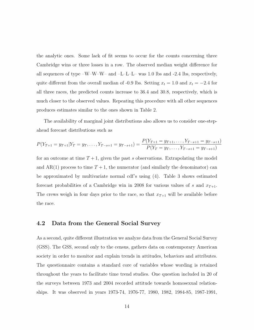
the analytic ones. Some lack of fit seems to occur for the counts concerning three

Cambridge wins or three losses in a row. The observed median weight difference for

all sequences of type –W–W–W– and –L–L–L– was 1.0 lbs and -2.4 lbs, respectively,

quite different from the overall median of -0.9 lbs. Setting xt = 1.0 and xt = −2.4 for

all three races, the predicted counts increase to 36.4 and 30.8, respectively, which is

much closer to the observed values. Repeating this procedure with all other sequences

produces estimates similar to the ones shown in Table 2.

The availability of marginal joint distributions also allows us to consider one-step-

ahead forecast distributions such as

P (YT+1 = yT+1|YT = yT , . . . , YT−s+1 = yT−s+1) =P (YT+1 = yT+1, . . . , YT−s+1 = yT−s+1)

P (YT = yT , . . . , YT−s+1 = yT−s+1)

for an outcome at time T +1, given the past s observations. Extrapolating the model

and AR(1) process to time T + 1, the numerator (and similarly the denominator) can

be approximated by multivariate normal cdf’s using (4). Table 3 shows estimated

forecast probabilities of a Cambridge win in 2008 for various values of s and xT+1.

The crews weigh in four days prior to the race, so that xT+1 will be available before

the race.

4.2 Data from the General Social Survey

As a second, quite different illustration we analyze data from the General Social Survey

(GSS). The GSS, second only to the census, gathers data on contemporary American

society in order to monitor and explain trends in attitudes, behaviors and attributes.

The questionnaire contains a standard core of variables whose wording is retained

throughout the years to facilitate time trend studies. One question included in 20 of

the surveys between 1973 and 2004 recorded attitude towards homosexual relation-

ships. It was observed in years 1973-74, 1976-77, 1980, 1982, 1984-85, 1987-1991,

14

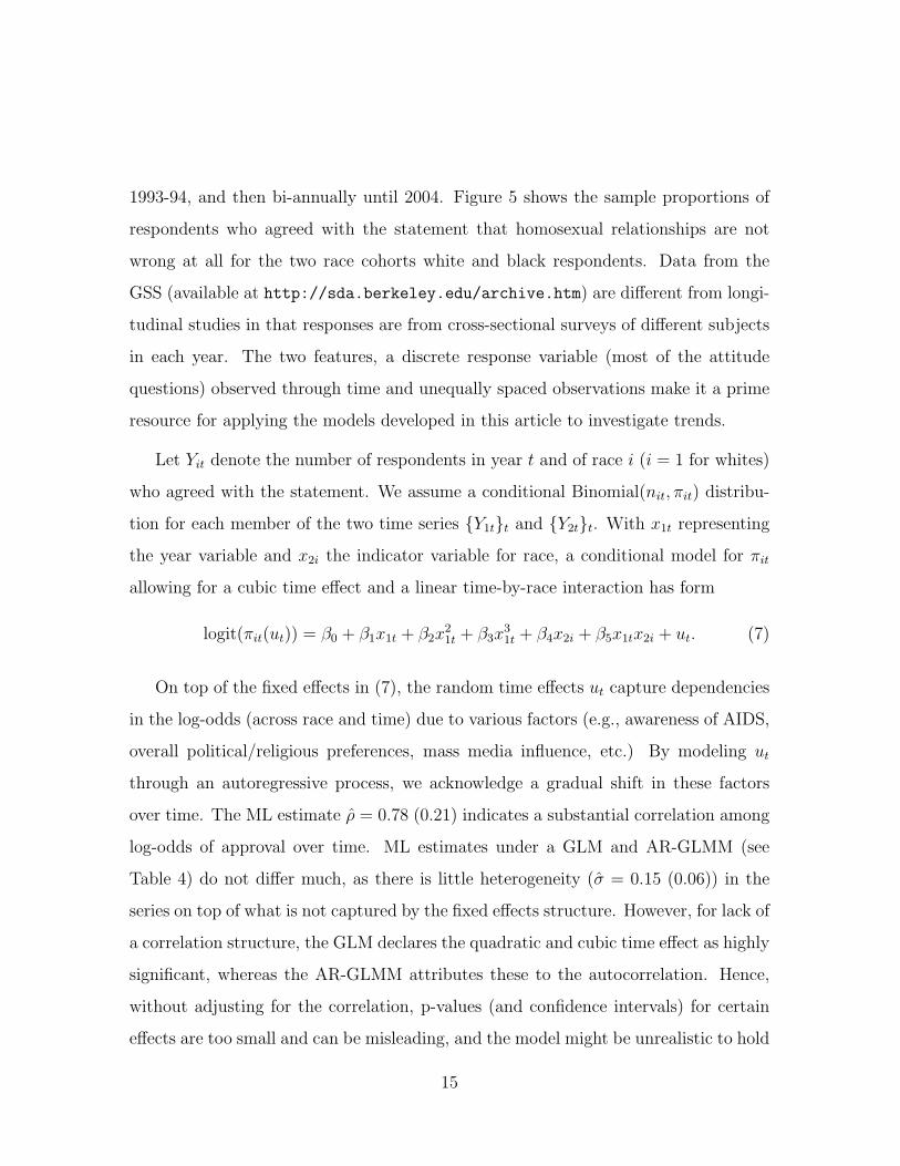
1993-94, and then bi-annually until 2004. Figure 5 shows the sample proportions of

respondents who agreed with the statement that homosexual relationships are not

wrong at all for the two race cohorts white and black respondents. Data from the

GSS (available at http://sda.berkeley.edu/archive.htm) are different from longi-

tudinal studies in that responses are from cross-sectional surveys of different subjects

in each year. The two features, a discrete response variable (most of the attitude

questions) observed through time and unequally spaced observations make it a prime

resource for applying the models developed in this article to investigate trends.

Let Yit denote the number of respondents in year t and of race i (i = 1 for whites)

who agreed with the statement. We assume a conditional Binomial(nit, πit) distribu-

tion for each member of the two time series {Y1t}t and {Y2t}t. With x1t representing

the year variable and x2i the indicator variable for race, a conditional model for πit

allowing for a cubic time effect and a linear time-by-race interaction has form

logit(πit(ut)) = β0 + β1x1t + β2x21t + β3x

31t + β4x2i + β5x1tx2i + ut. (7)

On top of the fixed effects in (7), the random time effects ut capture dependencies

in the log-odds (across race and time) due to various factors (e.g., awareness of AIDS,

overall political/religious preferences, mass media influence, etc.) By modeling ut

through an autoregressive process, we acknowledge a gradual shift in these factors

over time. The ML estimate ρ = 0.78 (0.21) indicates a substantial correlation among

log-odds of approval over time. ML estimates under a GLM and AR-GLMM (see

Table 4) do not differ much, as there is little heterogeneity (σ = 0.15 (0.06)) in the

series on top of what is not captured by the fixed effects structure. However, for lack of

a correlation structure, the GLM declares the quadratic and cubic time effect as highly

significant, whereas the AR-GLMM attributes these to the autocorrelation. Hence,

without adjusting for the correlation, p-values (and confidence intervals) for certain

effects are too small and can be misleading, and the model might be unrealistic to hold

15

outside the observation window. For instance, over the period of 20 years from 1984

to 2004, the estimated marginal odds of approval increased by a factor of 2.5 (95%

C.I.: [1.77, 3.25]) for white respondents and by a factor of 1.7 [1.17, 2.41] for black

respondents. These estimates are based on the MLEs for the AR-GLMM without

the insignificant quadratic and cubic effect (see Table 4). The point estimate and

confidence intervals are shifted and wider than their GLM counterparts of [3.03, 3.88]

and [1.94, 3.08], respectively, which is mostly due to the fact that the ratio of the

estimate of β1 to its s.e. is 2.7 times larger under the AR-GLMM. The marginal odds

of approval for white respondents in 1984 are estimated to be 1.36 [1.27, 1.61] times

those for black respondents in that year. Twenty years later, in 2004, this factor

increases to 2.04 [1.69, 2.47]. As these contrasts don’t involve the quadratic or cubic

effects, results are similar to a GLM. Finally, the estimated odds of approval for black

respondents in 2004 are almost equal to the estimated odds for white respondents 16

years back in 1988.

Since sample sizes nit are large for these data, a normal approximation of the log

odds could be sensitive. However, the right panel in Figure 5 clearly shows the non-

constant behavior of the empirical standard deviations [nitpit(1 − pit)]−1/2 of the log

odds, where pit = yit/nit are the sample proportions. This is due to the trend in the

probabilities (sample proportions range from 0.05 to 0.35) and non-constant sample

sizes (e.g., n1t is much larger than n2t and only half as many subjects were sampled in

1988 to 1993). For fitting a normal linear mixed model (LMM), we therefore introduce

weights ωit which are the inverse of these empirical standard deviations and model the

standardized log-odds (we fix the residual standard error from the normal mixed model

at 1). Such weighted LMM can be fitted in e.g., SAS, which also allows for unequally

spaced autocorrelated random effects. Estimates in Table 4 show that results are

almost identical to the AR-GLMM analysis, albeit computationally much simpler to

obtain. However, the inability of the LMM to model the variance as a function of

16

the mean (which we circumvented by considering standardized log-odds) renders this

model class not suitable for analyzing binomial time series in general.

5 Summary and Discussion

Ignoring correlation in discrete time series can lead to wrong inference (based on wrong

standard errors) which was apparent for the two examples and the simulations. At

the cost of increased computational time and complex algorithms (MCEM with Gibbs

sampling), we based inferential procedures for AR-GLMMs on the joint likelihood of

the T serially correlated observation, leading to efficient estimation and enabling ap-

proximations to marginal higher-order moments. These are useful for assessing the

parametric correlation assumption, constructing tables for checking the fit and pre-

dicting future observations. Further, our models and estimation routines are flexible

enough to handle gaps in the series without any additional procedures or adjustments,

such as ignoring the gaps and artificially treating the series as equally spaced or try-

ing to impute values. Unlike GEE, our methodology should be practical when not all

subjects are measured at common time points or missing at random.

It is not accidental that certain sequences, such as –W–L– and –L–W– or –W–W–

L– and –L–W–W– in Table 2 have equal expected marginal probabilities (and hence

predicted counts) when a time dependent covariate is held at a constant level. This

is due to the symmetry in the bi- and trivariate normal distribution of (ut−1, ut) and

(ut−2, ut−1, ut) which dictates that φ2(ut−1, ut) ≡ φ2(ut, ut−1) and φ3(ut−2, ut−1, ut) ≡φ3(ut, ut−1, ut−2), where φk is the k-dim. normal density of {ul}t

l=t−k, k = 2, 3. (Note,

however, that φ3(ut−2, ut−1, ut) 6= φ3(ut−2, ut, ut−1) and hence sequences –W–W–L–

and –W–L–W– are not modeled as exchangeable. They, indeed, have a different

dynamical structure.) Hence, AR-GLMMs for binary time series possess reasonable

17

exchangeability properties for certain sequences of successes and failures when the

mean is held constant.

In an influential article in the political science literature, Beck et al. (1998) include

dummy variables or cubic splines to model temporal association in binary time series

cross-sectional data, but note that this “cannot provide a satisfactory explanation

[of an event] by itself, but must, instead, be the consequence of some important, but

unobserved, variable”. AR-GLMMs, which have less stringent assumptions and model

this unobserved variable seem to be an attractive alternative.

Acknowledgements

The author would like to thank Drs. Agresti, Booth and Casella for serving on

his Ph. D. committee under which part of this work was done. Most computations

and graphs were carried out in the fast program language OX, developed by Jurgen

Doornik at the Univ. of Oxford.

18

Appendix A: Generating Samples from h(u|y)

Let yt = (y1t, . . . , ykt) denote the vector of i = 1, . . . , k binomial (nit, πit(ut)) obser-

vations at time point t. For a single binary time series, k = 1 and n1t = 1 for all t.

In the following, we suppress dependencies on parameters β and ψ as densities are

always evaluated at their current estimates. The full univariate conditionals for the

AR(1) random effects depend only on their immediate neighbors ut−1 and ut+1, i.e.,

g(ut|u1, . . . , ut−1, ut+1, . . . , uT ) ∝ g(ut|ut−1)g(ut+1|ut), t = 2, . . . , T − 1, and, for t = 1

and t = T , only on u2 and uT−1, respectively. The full univariate conditionals can

be expressed as ht(ut|ut−1, ut+1, yt) ∝ f(yt|ut) gt(ut|ut−1, ut+1), where, using standard

multivariate normal theory results,

g1(u1|u2) = N(ρd1u2, σ

2[1− ρ2d1 ])

gt(ut|ut−1, ut+1) = N

(ρdt−1 [1− ρ2dt−1 ]ut−1 + ρdt [1− ρ2dt−1 ]ut+1

1− ρ2(dt−1+dt),

σ2[1− ρ2dt−1 − ρ2dt + ρ2(dt−1+dt)]

1− ρ2(dt−1+dt)

), t = 2, . . . , T − 1

gT (uT |uT−1) = N(ρdT−1uT−1, σ

2[1− ρ2dT−1 ]).

For equally spaced data (without loss of generality dt = 1 for all t) these distributions

reduce to the ones derived in Chan and Ledolter (1995).

Direct sampling from ht is not possible. However, it is straightforward to imple-

ment an accept-reject algorithm with candidate density gt, since ht/gt < L(yt) with

L(yt) =∏k

i=1(yit/nit)yit(1 − yit/nit)

nit−yit . Given u(j−1) =(u

(j−1)1 , . . . , u

(j−1)T

)from

the previous iteration, the Gibbs sampler with accept-reject sampling from the full

univariate conditionals generates components u(j)t ∼ ht(u

(j)t |u(j)

t−1, u(j−1)t+1 ,yt) through

generating ut from candidate density gt(ut|u(j)t−1, u

(j−1)t+1 ) and w ∼ Unif[0, 1] and then

setting u(j)t = ut if w ≤ f(yt|ut)/L(yt) or repeating the process otherwise. The sample

u(1), . . . , u(m) (after allowing for burn-in) is then used to approximate the E-step in

the kth- iteration of the MCEM algorithm.

19

Appendix B: MLEs for σ and ρ for unequally spaced time series

For unequally spaced AR(1) random effects and a sample u(1), . . . , u(m) from h(u|y),

Q2m has form

Q2m(σ, ρ) ∝ −T log σ − 1

2

T−1∑t=1

log(1− ρ2dt)− 1

2σ2

1

m

m∑j=1

u(j)1

2

− 1

2σ2

1

m

m∑j=1

T−1∑t=1

[u

(j)t+1 − ρdtu

(j)t

]2

1− ρ2dt,

where u(j)t is the t-th component of the j-th sampled vector u(j). Denote the parts

depending on ρ and the generated sample u(1), . . . , u(m) by

at(ρ, u) =1

m

m∑j=1

(u

(j)t+1 − ρdtu

(j)t

)2

and bt(ρ,u) =1

m

m∑j=1

(u

(j)t+1 − ρdtu

(j)t

)u

(j)t .

Then the MLE of σ at iteration k of the MCEM algorithm has form

σ(k) =

(1

Tm

m∑j=1

u(j)1

2+

1

T

T−1∑t=1

1

1− ρ2dtat(ρ, u)

)1/2

.

No closed form solutions exist for ρ(k) when random effects are unequally spaced. Let

ct(ρ) =dtρ

dt−1

1− ρ2dtand et(ρ) =

ρ

dt

[ct(ρ)]2

be terms depending on ρ but not on u. Then,

∂

∂ρQ2

m =T−1∑t=1

ρdtct(ρ) +1

σ2

T−1∑t=1

[ct(ρ)bt(ρ, u)− et(ρ)at(ρ,u)] .

Since the range of ρ is restricted to (−1, 1), we suggest the simple interval-halving

method on ∂∂ρ

Q2m|σ=σ(k) to find the root ρ(k). For the special case of equidistant time

points, all dt are equal and ρ(k) is the closed-form solution of a third degree polynomial.

20

References

Beck, N., Katz, J. N., Tucker, R., 1998. Taking time seriously: Time-serious-cross-

section analysis with a binary dependent variable. Amer. J. Political Science 42,

1260–1288.

Benjamin, M. A., Rigby, R. A., Stasinopoulos, M. D., 2003. Generalized autoregressive

moving average models. J. Amer. Statist. Assoc. 98, 214–223.

Booth, J. G., Hobert, J. P., 1999. Maximizing generalized linear mixed model likeli-

hoods with an automated Monte Carlo EM algorithm. J. Roy. Statist. Soc. Ser. B

61, 265–285.

Chan, K. S., Ledolter, J., 1995. Monte Carlo EM estimation for time series models

involving counts. J. Amer. Statist. Assoc. 90, 242–252.

Chen, M.-H., Ibrahim, J., 2000. Bayesian predictive inference for time series count

data. Biometrics 56, 678–685.

Chib, S., Greenberg, E., 1998. Analysis of multivariate probit models. Biometrika 85,

347–361.

Czado, C., 2000. Multivariate regression analysis of panel data with binary outcomes

applied to unemployment data. Statist. Papers 41, 281–304.

Davis, R. A., Dunsmuir, W. T. M., Streett, S. B., 2000. On autocorrelation in a

Poisson regression model. Biometrika 87, 491–505.

Davis, R. A., Rodriquez-Yam, G., 2005. Estimation of state-space models; an approx-

imate liklihood approach. Statist. Sinica 15, 381–406.

Demidenko, E., 2004. Mixed Models: Theory and Applications. Wiley, New York.

21

Diggle, P., Heagerty, P., Liang, K.-Y., Zeger, S. L., 2002. Analysis of Longitudinal

Data, 2nd Edition. Oxford University Press, Oxford.

Durbin, J., Koopman, S. J., 2000. Time series analysis of non-Gaussian observations

based on state space models from both classical and Bayesian perspectives. J. Roy.

Statist. Soc. Ser. B 62, 3–56.

Durbin, J., Koopman, S. J., 2001. Time Series Analysis by State Space Methods.

Oxford: Oxford University Press.

Fahrmeir, L., Tutz, G., 2001. Multivariate Statistical Modelling Based on Generalized

Linear Models, 2nd Edition. Springer, New York.

Fitzmaurice, G. M., Laird, N. M., Ware, J. H., 2004. Applied Longitudinal Analysis.

Wiley, Hoboken, N.J.

Fokianos, K., Kedem, B., 2004. Partial likelihood inference for time series following

generalized linear models. J. Time Ser. Anal. 25, 173–197.

Hay, J. L., Pettitt, A., 2001. Bayesian analysis of time series of counts. Biostatistics

2, 433–444.

Heagerty, P. J., Zeger, S. L., 1998. Lorelogram: A regression approach to exploring

dependence in longitudinal categorical responses. J. Amer. Statist. Assoc. 93 (441),

150–162.

Jung, R. C., Kukuk, M., Liesenfeld, R., 2006. Time series of counts data: modeling,

estimation and diagnostics. Comput. Statist. Data Anal. 51, 2350–2364.

Kedem, B., Fokianos, K., 2002. Regression Models for Time Series Analysis. Wiley,

New York.

22

Kuk, A. Y. C., Cheng, Y. W., 1999. Pointwise and functional approximations in Monte

Carlo maximum likelihood estimation. Statist. and Comput. 9, 91–99.

Lee, Y., Nelder, J. A., 2004. Conditional and marginal models: Another view. Statist.

Science 19, 219–238.

Li, W. K., 1994. Time series models based on generalized linear models: Some further

results. Biometrics 50, 506–511.

Liu, S.-I., 2001. Bayesian model determination for binary-time-series data with appli-

cations. Comput. Statist. Data Anal. 36, 461–473.

Louis, T. A., 1982. Finding the observed information matrix when using the EM

algorithm. J. Roy. Statist. Soc. Ser. B 44, 226–233.

MacDonald, I. L., Zucchini, W., 1997. Hidden Markov and other Models for Discrete-

Valued Time Series. Chapman & Hall, New York.

Molenberghs, G., Verbeke, G., 2007. Likelihood ratio, score and Wald tests in a con-

strained parameter space. The Amer. Statist. 61, 22–27.

Newton, M. A., Raftery, A. E., 1994. Approximate Bayesian inference with the

weighted likelihood bootstrap. J. Roy. Statist. Soc. Ser. B 56, 3–48.

Pettitt, A., Weir, I., Hart, A., 2002. A conditional autoregressive Gaussian process

for irregularly spaced multivariate data with application to modelling large sets of

binary data. Statist. and Comput. 12, 353–367.

Renard, D., Molenberghs, G., Geys, H., 2004. A pairwise likelihood approach to esti-

mation in multilevel probit models. Comput. Statist. Data Anal. 44, 649–667.

Stram, D. O., Lee, J. W., 1994. Variance components testing in the longitudinal mixed

effects model. Biometrics 50, 1171–1177.

23

Sun, D., Speckman, P. L., Tsutakawa, R. K., 2000. Random effects in generalized

linear mixed models. In: Dey, D., Ghosh, S., Mallick, B. (Eds.), Generalized Linear

Models: A Bayesian perspective. Marcel-Dekker, New York.

Sun, D., Tsutakawa, R. K., Speckman, P. L., 1999. Posterior distribution of hierar-

chical models using CAR(1) distributions. Biometrika 86, 341–350.

Varin, C., Vidoni, P., 2006. Pairwise likelihood inference for ordinal categorical time

series. Comput. Statist. Data Anal. 51, 2365–2373.

Wei, G. C. G., Tanner, M. A., 1990. A Monte Carlo implementation of the EM

algorithm and the poor man’s data augmentation algorithms. J. Amer. Statist.

Assoc. 85, 699–704.

Zeger, S. L., 1988. A regression model for time series of counts. Biometrika 75, 621–

629.

24

Table 1: A simulation study to assess properties of the proposed MCEM algorithm

and compare standard errors (s.e.) from GLM and AR-GLMM fits. For each set of

true parameters, 100 binary time series with T = 152 and 27 random gaps of size dt

from 2 to at most 6 were generated according to the model logit[πt(ut)] = α+βxt +ut,

with xt ∼ N(0, 1) and ut+1 = ρdt ut + εt, εt ∼ N(0, σ2[1− ρ2dt ]). Avg. and Std. denote

simulation average and standard deviation.

α β σ ρ s.e.(α) s.e.(β) s.e.(σ) s.e.(ρ)

True: 1 1 2 0.8

GLM Avg.: 0.62 0.66 0.18 0.21

Std.: 0.30 0.21 0.01 0.02

AR-GLMM Avg.: 1.01 1.08 2.08 0.76 0.65 0.42 1.03 0.15

Std.: 0.51 0.37 0.65 0.16 0.34 0.22 0.68 0.21

True: 1 1 2 0.5

GLM Avg.: 0.64 0.65 0.20 0.20

Std.: 0.25 0.26 0.01 0.02

AR-GLMM Avg.: 0.98 1.04 2.09 0.46 0.63 0.48 0.92 0.21

Std.: 0.54 0.36 0.59 0.21 0.25 0.26 0.71 0.18

True: 1 1 1.5 0.8

GLM Avg.: 0.79 0.76 0.19 0.21

Std.: 0.33 0.24 0.02 0.02

AR-GLMM Avg.: 1.05 1.04 1.54 0.78 0.56 0.44 0.61 0.14

Std.: 0.49 0.34 0.44 0.15 0.23 0.14 0.49 0.11

True: 1 1 1.5 0.5

GLM Avg.: 0.78 0.75 0.20 0.21

Std.: 0.21 0.21 0.01 0.02

AR-GLMM Avg.: 0.95 0.97 1.42 0.47 0.51 0.41 0.64 0.22

Std.: 0.45 0.31 0.39 0.19 0.12 0.16 0.47 0.43

Note: Starting values for fixed effects were regular GLM estimates and for σ and ρ thevariance and correlation of the empirical log-odds. For 4 of the 100 generated time series,the Monte Carlo sample size at parameter convergence was not large enough to give a positivedefinite estimate of the covariance matrix. In these cases, the algorithm continued until apositive definite estimate was found. The median Monte Carlo sample size at convergencewas 9683 (IQR: 12,945). The median computation time to convergence was 1.2 hours (IQR:3 hours) on a Pentium 4 processor with 2Ghz of RAM.

25

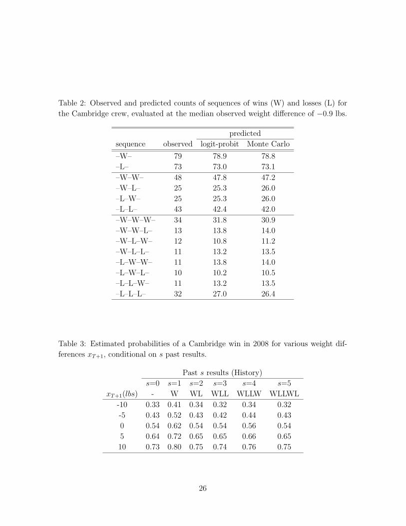
Table 2: Observed and predicted counts of sequences of wins (W) and losses (L) for

the Cambridge crew, evaluated at the median observed weight difference of −0.9 lbs.

predicted

sequence observed logit-probit Monte Carlo

–W– 79 78.9 78.8

–L– 73 73.0 73.1

–W–W– 48 47.8 47.2

–W–L– 25 25.3 26.0

–L–W– 25 25.3 26.0

–L–L– 43 42.4 42.0

–W–W–W– 34 31.8 30.9

–W–W–L– 13 13.8 14.0

–W–L–W– 12 10.8 11.2

–W–L–L– 11 13.2 13.5

–L–W–W– 11 13.8 14.0

–L–W–L– 10 10.2 10.5

–L–L–W– 11 13.2 13.5

–L–L–L– 32 27.0 26.4

Table 3: Estimated probabilities of a Cambridge win in 2008 for various weight dif-

ferences xT+1, conditional on s past results.

Past s results (History)

s=0 s=1 s=2 s=3 s=4 s=5

xT+1(lbs) - W WL WLL WLLW WLLWL

-10 0.33 0.41 0.34 0.32 0.34 0.32

-5 0.43 0.52 0.43 0.42 0.44 0.43

0 0.54 0.62 0.54 0.54 0.56 0.54

5 0.64 0.72 0.65 0.65 0.66 0.65

10 0.73 0.80 0.75 0.74 0.76 0.75

26

Table 4: MLEs for modeling the log-odds of approval in the GSS data set via a

GLM and AR-GLMM. Results are also displayed for fitting a linear mixed model

with autocorrelated random effects (AR-LMM) to the standardized log-odds. The

last two columns present the result of the AR-LMM and AR-GLMM when dropping

the insignificant quadratic and cubic time effect.

GLM AR-LMM AR-GLMM AR-LMM AR-GLMM

β0 -1.53 (0.03) -1.49 (0.10) -1.49 (0.19) -1.38 (0.11) -1.38 (0.09)

β1 0.95 (0.07) 0.81 (0.22) 0.80 (0.24) 0.65 (0.13) 0.66 (0.14)

β2 0.33 (0.05) 0.22 (0.15) 0.20 (0.29) − −β3 -0.32 (0.09) -0.16 (0.24) -0.15 (0.27) − −β4 -0.46 (0.05) -0.43 (0.05) -0.45 (0.05) -0.43 (0.05) -0.45 (0.05)

β5 -0.25 (0.08) -0.30 (0.09) -0.27 (0.08) -0.29 (0.09) -0.27 (0.08)

σ − 0.15 (0.04) 0.15 (0.06) 0.19 (0.02) 0.19 (0.07)

ρ − 0.77 (0.15) 0.78 (0.21) 0.86 (0.09) 0.86 (0.10)

27

Figure 1: Conditional (grey) and marginal (black) success probabilities based on logit

(solid) and scaled probit (dashed) links, for linear predictor values ranging from -6 to

6. Each pair of grey (solid,dashed)-curves in each panel corresponds to one out of 6

randomly sampled random effects zt. The two black lines in each panel represent the

implied marginal probability, the true one (obtained by a Monte Carlo sum, averaging

over 100,000 randomly sampled zt’s) represented as a solid line, and the one based

on approximation (4) by a dashed one. The four panels correspond to four different

values of the random effects standard deviation, σ = 1, 1.5, 2 and 2.5.

−5.0 −2.5 0.0 2.5 5.0

0.25

0.50

0.75

1.00σ= 1

−5.0 −2.5 0.0 2.5 5.0

0.25

0.50

0.75

1.00σ= 1.5

−5.0 −2.5 0.0 2.5 5.0

0.25

0.50

0.75

1.00σ= 2

−5.0 −2.5 0.0 2.5 5.0

0.25

0.50

0.75

1.00σ= 2.5

28

Figure 2: Plot of the Oxford vs. Cambridge boat race data. Observed series (first

panel, 1 denotes a Cambridge win, 0 a loss) and estimated conditional (second panel)

and marginal (third panel) probabilities of a Cambridge win.

1840 1860 1880 1900 1920 1940 1960 1980 2000

0.5

1.0

1840 1860 1880 1900 1920 1940 1960 1980 2000

0.5

1.0

π t

1840 1860 1880 1900 1920 1940 1960 1980 2000

0.5

1.0

π tm

29

Figure 3: Comparison of sample and model based Lorelogram.

1 3 5 7 9 11 13 15

−0.25

0.00

0.25

0.50

0.75

1.00

1.25

1.50

Lorelogram

Log−

odds

Rat

io

Lag

Smooth Sample Sample

Model 2 × ASE

30

Figure 4: Estimated marginal probabilities P (Yt = yt, Yt+1 = yt+1) of two successive

Cambridge wins (–W–W–), a win and a loss (–W–L–), a loss and a win (–L–W–) and

two Cambridge losses in a row (–L–L–), for combination of crew weight differences

(xt, xt+1) ranging from (-15,-15) lbs to (15,15) lbs. The probability axis (labeled Prob.)

ranges from 0 to 1.

xtxt+1

Prob.

−W−W−

xtxt+1

Prob.

−W−L−

xtxt+1

Prob.

−L−W−

xtxt+1

Prob.

−L−L−

31

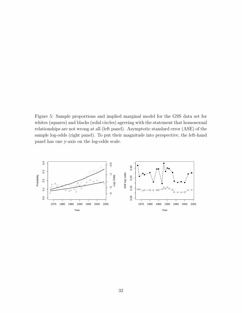
Figure 5: Sample proportions and implied marginal model for the GSS data set for

whites (squares) and blacks (solid circles) agreeing with the statement that homosexual

relationships are not wrong at all (left panel). Asymptotic standard error (ASE) of the

sample log-odds (right panel). To put their magnitude into perspective, the left-hand

panel has one y-axis on the log-odds scale.

1975 1980 1985 1990 1995 2000 2005

0.0

0.1

0.2

0.3

0.4

Year

Pro

babi

lity

−3

−2

−1

−0.

5Lo

g−O

dds

1975 1980 1985 1990 1995 2000 2005

0.00

0.10

0.20

0.30

Year

AS

E lo

g−od

ds

32