REGIONAL VARIATION IN WORK ABSENCE CULTURES

IN THE UNITED STATES

BY

JORGE IVAN HERNANDEZ

DISSERTATION

Submitted in partial fulfillment of the requirements

for the degree of Doctor of Philosophy in Psychology

in the Graduate College of the

University of Illinois at Urbana-Champaign, 2015

Urbana, Illinois

Doctoral Committee:

Associate Professor Daniel A. Newman, Chair

Professor Dov Cohen

Professor James Rounds

Associate Professor Patrick Vargas

Professor Emeritus Charles L. Hulin

ii

ABSTRACT

This paper offers a cultural perspective to the work absenteeism literature, by conceptualizing

work absence at the U.S. state level of analysis, and by assessing absenteeism as a manifestation

of regional cultures. First, I establish that absenteeism is a spatially dependent phenomenon, and

demonstrate that the retest reliability of absenteeism increases at higher levels of aggregation

(from individual-level to city-level to state-level), to provide evidence for absence as a state-level

construct. Second, I hypothesize main effects of regional cultures on state-level work

absenteeism (i.e., in the U.S. West). Third, I assess whether observed regional differences in

state-level absence cultures in the West are attributable to (mediated by) regional differences in

state-level social disorganization/anomie, while controlling for state-level variance in work

industry (e.g., manufacturing), personality (Extraversion, Neuroticism), unemployment rates, and

physical disabilities. Analyzing data spanning over 4 years and over 3 million people per year,

this paper explains how absenteeism varies across states in the U.S.

iii

TABLE OF CONTENTS

CHAPTER 1: INTRODUCTION ................................................................................................ 1

CHAPTER 2: METHOD .............................................................................................................21

CHAPTER 3: RESULTS .............................................................................................................30

CHAPTER 4: REPLICATION OF STATE-LEVEL EFFECTS AT THE CITY LEVEL ............33

CHAPTER 5: DISCUSSION .......................................................................................................39

REFERENCES ............................................................................................................................45

FIGURES AND TABLES ............................................................................................................58

1

CHAPTER 1

INTRODUCTION

Absenteeism is commonly defined as the failure to report for scheduled work over a

given time interval (Johns, 1995). From an economic perspective, absenteeism leads to large

financial losses in companies. For example, total absenteeism has been estimated to represent

roughly 5.8% of payroll (Kronos Incorporated, 2010), with estimated costs on the order of $650

to $850 per employee per year just for sickness absenteeism alone (Barham & Leonard, 2002). In

addition to the cost of accommodating absent employees, the employees left behind to do the

work are 21-29% less efficient (Kronos Incorporated, 2014). In all, productivity losses from

absenteeism in the United States have been estimated in the hundreds of billions of dollars (e.g.,

$225.8 billion per year; Stewart, Ricci, Chee, Hahn, & Morganstein, 2003). Further, in a national

survey, 33%of responding organizations reported that absenteeism was a “serious problem”

(CCH Incorporated, 2006). Beyond these practical considerations, research that enhances our

understanding of the antecedents of absenteeism will advance basic science in the domain of

organizational behavior.

The current paper proposes to make three contributions to the study of regional variation

in work absenteeism in the U.S. First, I seek to establish the existence of reliable variation in

workplace absence at the U.S. state level of analysis. Second, I test whether state-level absence

displays geographic regional variation, with absenteeism concentrated in the Western U.S. Third,

I propose that the tendency for Western states to exhibit higher absenteeism rates can be

explained by the relatively high levels of social disorganization/anomie in the U.S. West.

2

Theoretical Models of Absence

One of the most influential theoretical frameworks used to explain absenteeism is the

Steers and Rhodes (1978; Rhodes & Steers, 1990) model. This model specifies that absenteeism

is most proximally influenced by the interaction between two factors—attendance ability and

attendance motivation. The first factor, ability to attend, was conceptualized for the purpose of

distinguishing voluntary from involuntary absence, and is exemplified by three categories of

variables: (a) sickness and accidents, (b) family responsibilities, and (c) transportation problems.

The second factor, attendance motivation, is proposed to be driven by two factors (a) job

satisfaction (which is the result of job situation characteristics like the scope, level, and

experienced stress of a job), and (b) pressures to attend (including economic/market conditions,

incentives/rewards, work group norms, organizational commitment, and personal work ethic). A

key implication of the Steers and Rhodes model is the necessity, but not sufficiency, of

attendance motivation. Employees with the motivation to attend are more likely to attend,

provided they also have the ability to attend.

This classic model of absenteeism underscored the complexity of attendance behavior,

emphasizing that it is a multiply-determined behavior, which incorporates concepts from a

variety of disciplines. Although the larger model itself has not been tested in its entirety, several

of its premises stimulated research (for a review, see Rhodes & Steers, 1990). Many of the

proposed antecedents in the model have been the focus of subsequent investigation.

Indeed, most of the central variables in Steers and Rhodes’ (1978) model have some

empirical support as predictors of absenteeism. Job satisfaction is one of the most commonly

studied variables in the absenteeism literature (Hackett, 1989; Harrison, Newman, & Roth,

2006), where it is posited that absenteeism is a response to negative job attitudes (March &

3

Simon, 1958). Empirical studies have found mixed support for the job satisfaction-absenteeism

link, with the overall meta-analytic effect size between rcorrected = -0.21 and -0.11; (Hackett, 1989;

McShane, 1984, Scott & Taylor, 1985). Related to job satisfaction, the rewards one receives from

the organization, as well as workplace characteristics, are suggested in the Steers and Rhodes

model to also affect absenteeism. Social exchange theory (Blau, 1964; Cropanzano & Mitchell,

2005; Gouldner, 1960; Thibault & Kelley, 1959) has been used to argue that the rewards and

costs an employee receives affect one’s organizational contributions. One example of how social

exchange theory explains absenteeism is that an employees’ perceived organizational support

(POS) influences their absence frequency (Eisenberger, Huntington, Hutchison, Sowa,

Eisenberger, & Huntington, 1986). Further, the relationship between employees’ POS and

absenteeism is stronger for individuals with high exchange ideology (Hutchison & Sowa, 1986).

Still other research supports the importance of ability to attend, suggesting that

absenteeism is caused by people’s not being able to meet the physical/mental demands of their

work (Diestel & Schmidt, 2010; Schaufeli, Bakker, & Rhenen, 2009; Swider & Zimmerman,

2010). Supporting evidence finds that physical ailments such as lower back pain (r = .18;

Martocchio, Harrison, & Berkson, 2000) and illness (r = .14; Darr & Johns, 2008) increase

absence rates. Further, external factors such as greater travel distance and time from work

(Martin, 1971; Stockford, 1944, Knox, 1961) are associated with higher rates of absenteeism.

Nonetheless, Steers and Rhodes’ (1978) proposed interaction effect, in which motivation to

attend is more predictive of attendance under conditions of high ability to attend, has not been

clearly supported. Perhaps one reason for this unsupported interaction effect is indicated in

Smith’s (1977) classic finding that, when absence was measured on the day after a major

snowstorm (i.e., when perceived ability to attend was low) department-level job satisfaction

4

facets correlated between r = .4 and r = .6 with department-level attendance. This finding

suggests that motivation to attend can sometimes be more predictive of attendance when ability

to attend is low, not high (contrary to Steers and Rhodes’ prediction). One possible reason for

this finding is that, when ability to attend is low, then attendance norms are relaxed (i.e., a weak

situation/low situational constraint; Herman, 1973) and job attitudes become a more important

driver of attendance behavior.

In addition to the above motivational and ability explanations, absenteeism is also linked

to social norms of the office/team. That is, the collective/group-level attitudes toward absence in

an organization, or absence cultures (Hill & Trist, 1955), may influence individual employee

attendance. A variety of research finds that employees’ initial estimates of their groups’

absenteeism rates (as well as their groups’ actual absenteeism rates) predict future individual-

level absence, above and beyond prior individual absenteeism (Martocchio, 1992, Harrison &

Shaffer, 1994, Gellatly, 1995, Markham & McKee, 1995). Last, individual differences have also

been implicated in absenteeism (Steers & Rhodes, 1978). However, a meta-analysis by Salgado

(2002) finds that the Big Five personality traits exhibit near-zero relationships with

absenteeism—the most predictive traits being Conscientiousness (rcorrected = .06) and

Extraversion (rcorrected = -.08).

For the sake of completeness, I also mention that some scholars have conceptualized

absenteeism as a manifestation of a broader underlying construct of work withdrawal (Hanisch &

Hulin, 1990; 1991; Hanisch, Roznowski, & Hulin, 1998). According to these researchers,

absenteeism is part of a general syndrome of withdrawal behaviors, alongside lateness and break-

taking. Although lateness, absence, and turnover have been characterized as common responses

to a dissatisfying work situation (Hulin, 1991), more recent meta-analytic evidence suggests that

5

the bivariate relationships amongst these so-called withdrawal behaviors cannot be accounted for

by their common association with job satisfaction (Berry, Lelchook, & Clark, 2012). Indeed, it is

plausible that the absence construct plays a role in a progression-of-withdrawal pattern (Rosse &

Miller, 1984), such that absence resides in a sequentially intermediate role between lateness and

turnover (i.e., lateness leads to increased absence, which leads to increased probability of

turnover; Berry et al., 2012; Harrison et al., 2006).

Group-level Absenteeism

Whereas most previous studies have conceptualized absenteeism as an individual-level

phenomenon, other researchers have proposed also treating it as a group-level phenomenon (for a

review of this literature, see Hausknecht, Hiller, & Vance, 2008). That is, the aggregate of

individual employee absences—averaged up to the level of the team, organization, firm, or

location/context--may represent its own distinct construct, with its own unique nomological

network. The process of moving a construct from a lower level of analysis up to a higher level of

analysis invokes a redefinition of that construct (Chan, 1998; Kozlowski & Klein, 2000;

Morgeson & Hofmann, 1999; Ostroff, 1993; Roberts, Hulin, & Rousseau, 1978; Thorndike,

1939).Once absenteeism is aggregated up to the unit level, we can no longer assume that it

occupies the same set of nomological relationships with other constructs—to do so would be to

commit an atomistic fallacy (Kozlowski & Klein, 2000; Robinson, 1950).

One benefit of studying absenteeism at a higher level of analysis is that it can provide

insights separate from individual-level absenteeism. This changes the focus to investigations of

group-level absenteeism rates and how they relate to various group characteristics. To date, there

is a small empirical literature supporting this distinction between the two concepts: individual

absence and unit-level absence. Terborg (1982) found that different retail stores, within the same

6

company, had significantly different levels of absence. Markham and McKee (1995) replicated

this finding, and in addition showed that different workplaces may have their own absenteeism

climates, where groups vary in terms of what they consider acceptable levels of absenteeism.

Chadwick-Jones, Nicholson, and Brown (1982) studied absenteeism rates in 16 different

organizations and found that the range of absence activity within each organization was restricted

relative to the range of absence activity between organizations. Collectively, these findings

suggest that absenteeism may not only be an individual-level construct, but also a distinct

construct at the group-level.

Because different workplaces can each have unique levels of absenteeism and

absenteeism norms, researchers have attempted to explain how this variance in absenteeism at

the group level of analysis arises. One proposed factor is normative social influence. This

explanation suggests that people conform to the behaviors of others because they want to be

liked and accepted by them. Referred to as the ‘deviance model’ of absenteeism (Johns, 1997), it

suggests that absenteeism can be viewed negatively by an entire group, and to avoid the negative

evaluation, all individuals experience a pressure to act similarly to each other. Indeed, Nicholson

(1975) found that negative stereotypes of other people's absence were widely held. Also

consistent with a deviance model, people tend to underreport their own actual absences, and to

see their attendance records as superior to those of their coworkers (Harrison & Shaffer, 1994).

Further, Gellatly (1995) found that perceived absence norms of a group (measured by asking

employees from 13 nursing units to estimate the average numbers of days people were absent)

predicted individual level absence in the future (r = .35), even after controlling for current levels

of absence. As mentioned previously, other research finds similar associations between the

perceived absence in an organizational unit and subsequent absenteeism of an individual

7

(Martocchio, 1992, Harrison & Shaffer, 1994, Markham & McKee, 1995). Additionally, in a

social network study using a classroom sample, the prior absences of one's friends predicted

one's own absences during subsequent weeks (r = .33, Yu & Newman, 2006). The study also

found that those students with perfect attendance had higher centrality in the network, and those

with lower rates of attendance were more likely to be on the periphery. In sum, these results

suggest one possible origin of group-level absenteeism: group-differences of absence may arise

partly from the social influence of (and contagion among) close peers.

Another proposed factor is group mood or group affect. George (1990) hypothesized that

group-level absenteeism (averaged across an entire organization) can be affected by factors also

at the organizational level, such as how enjoyable it is to work in one organization compared to

another (i.e., collective mood). Thus, being in an organizational climate that is more positive may

be more rewarding for employees, compared to being in a group characterized by negative mood

states. Thus, according to George’s (1990) theoretical propositions, all employees in an office

can be subject to the same group-level affective influences, which should lead to more absences

for the office as a whole (i.e., meaningful between-group variance in absence taking). That is,

absenteeism at the aggregate level (i.e., the average absence frequency for an organization) is

predicted by the average negative tone of the individuals in that organization.

Multilevel Considerations for Group-level Absenteeism

Level of Aggregation.

Although several researchers have examined absenteeism at the group-level, these

researchers have varied in what level of aggregation they study. Most of the examples previously

discussed have occurred at either the organization-level or the team-level. Mathieu and Kohler

(1990) examined a cross-level model of individual-level absenteeism predicting that, in a small

8

sample of bus mechanics, city-level absence (which was confounded with organization-level

absence in their design) predicted individual absence, over and above prior individual-level

absence. That is, the average absence of a particular city/garage 6 months prior to the study

predicted the amount of time an individual lost 6 months later, even after accounting for the

individual’s previous absence time lost. These preliminary results open the possibility for models

of absenteeism that consider organization-level (and perhaps city-level) absence as its own

unique phenomenon.

Composition model for group-level absenteeism.

If one is to conceptualize absenteeism as a group-level construct, then a natural question

that emerges involves specifying the composition model for the group-level absence construct

(Chan, 1998; Kozlowski & Klein, 2000). According to Chan’s (1998) typology of composition

models, group-level constructs can be conceptualized using either a consensus model or an

additive model to compose the group-level concept. Defining a construct as emerging from either

a consensus model or additive model is important, because it implies the type of evidence that

would support whether the construct exists at the group-level.

Consensus models pertain to group-level constructs that require a high degree of within-

group agreement in order to claim that the group-level concept exists (James, Demaree, & Wolf,

1984; 1993; George & James, 1993). If the substantive definition of the construct involves some

form of collective judgment, evaluation, or perception, then a consensus model is implied by the

theory, and therefore a high level of within-group agreement is expected. Classic examples of

consensus models include organizational climate and team efficacy. These constructs exist at the

group level and require everyone within each distinct group to hold similar views to the other

group members. In contrast, an additive model is defined as a higher level construct that is a

9

summation of the lower level inputs. In these models, individual-level variability (i.e., within-

group agreement) is not a theoretical concern for justifying the existence of the aggregate-level

construct.

In the current paper, I conceptualize unit-level absenteeism as an additive construct

(Chan, 1998; cf. George & James, 1993), suggesting that the underlying phenomenon is

represented as the summation of individual behaviors, and occurs regardless of whether every

person engages in similar levels of the behavior. Similar to constructs such as organizational

sales performance, or the number of points scored by a basketball team, the notion of group

absence does not require that all members of a unit exhibit similar contributions or similar levels

of absence. Further, group-level constructs dealing with rare or highly skewed events may be

more appropriate for additive models, because high “agreement” (i.e., behavioral uniformity

across individuals within the group) is unlikely due to the low base rate/low frequency of the

event. As such, using an additive model is advantageous for studying deviant behaviors, due to

the low base rates of these behaviors. Previous research examining murders, domestic violence,

and rape at the group-level all treat the deviant construct as an additive model, where the

occurrences of the behavior within a unit do not need to be endorsed or performed in equal

amounts (i.e., within-group agreement is irrelevant to additive composition models of group-

level constructs).

Temporal Aggregation in Absenteeism.

In addition to aggregating absenteeism across individuals in the same organization or city

to form a group-level construct, aggregating over time also represents another level to be

considered. As one partial solution to the problem that absence tends to have a low base-rate and

is often severely skewed (Hammer & Landau, 1981), absenteeism researchers tend to aggregate

10

over longer time periods, such as an entire year (Mitra, Jenkins, & Gupta, 1992). Prior research

suggests that aggregating behavior over multiple occurrences increases the stability of the

measure, as well as the potential to detect systematic trends in the behavior, compared to when a

single instance of the behavior is used (Epstein, 1979). Epstein (1979) showed that when

behaviors such as self-ratings, emotion-ratings, heart rate, lateness, and many others were

measured each day for a month, the retest correlation between a participants’ scores on a

particular day and another day were much lower (typically only half as large) compared to when

the scores were averaged over longer periods (e.g., 6 odd-numbered days and 6 even-numbered

days). Increasing the aggregation interval (i.e., the temporal aggregation period) almost

invariably led to large increases in retest stability. Further, increasing periods of aggregation also

increased the probability of observing statistically significant correlations between the measures

and personality traits (Epstein 1979). Thus, single-time-point measures of behavior can be

expected, like single items in a test, to be low in reliability; which impairs the researcher’s ability

to adequately estimate relationships between that behavior and dispositions. (Epstein, 1980).In

situations where a single instance of behavior is expected to have a high level of measurement

error, aggregating over longer periods of time increases the ability to examine relationships with

that behavior, by avoiding unreliability attenuation. Behaviors such as absenteeism are a central

example, given that they have a low base rate and the underlying process is partially stochastic.

Therefore, both individual-level and group-level absenteeism may be better characterized when

these absenteeism rates are aggregated over longer periods of time. For the current project,

absenteeism will be examined at the highest level of aggregation possible (by averaging across

all time periods observed; i.e., averaging the 4 measures, taken across 4 years) to increase the

11

reliability and potential validity of the measure, as well as to reduce potential problems of low

base rate and skewness (see Hulin, 1991).

Current Theoretical Framework

The current paper proposes a framework that conceptualizes absenteeism as existing at

the group level of analysis, and specifies a unique set of precursors. Much of the previous work

on group-level absenteeism has examined other group-level predictors, such as workplace norms

and overall attitudes of the employees, to explain group-level absenteeism (see review above). In

contrast, the current paper will draw upon a deviance model from sociology, called social

disorganization theory (Shaw & McKay, 1942), to explain absenteeism rates at the U.S. state

level. Additionally, because social disorganization is tied to regional characteristics, this paper

proposes that there are distinct cultures of absenteeism across the U.S., where regions that are

more disorganized should have higher rates of absenteeism.

The social disorganization perspective of absenteeism extends a process commonly used

to described rates of deviant behavior in a community (e.g., violent crime, domestic abuse, arrest

rates), to include another form of deviant behavior, absenteeism (i.e., intentionally not fulfilling

workplace responsibilities). The contemporary social disorganization model says that three

community-level variables—residential mobility, family instability, and non-religiosity—lead to

more socially disorganized communities (Crutchfield, Geerken, and Grove, 1982; Petee &

Kowalski, 1993; Bouffard & Muftic, 2006). In a disorganized community, members lack a strong

sense of belonging to the community, receive less public scrutiny, and also feel a greater sense of

normlessness. As a result, the members are more likely to engage in deviant behavior. Because

absenteeism has negative effects for an entire group (e.g., a company, a city, a family), I suggest

that absenteeism is another example of community-related deviant behavior that could be

12

affected by the aforementioned conditions of social disorganization. Additionally, because of

geographic differences in social disorganization (i.e. the Western United States is more

disorganized compared to the Southern and Northern U.S.; as reviewed below), group-level

absenteeism is proposed to be a regional variable. Different regions of the United States will

have their own levels of disorganization, and these regional differences should lead to average

absenteeism rates that are similar to neighboring regions (as well as more distinct from farther

locations), producing regional variation in absenteeism.

Before I proceed to describe the tenets of the model, a caveat is in order. Although the

current model specifies group-level absenteeism as an outcome of social disorganization, another

possible explanation is that absenteeism is merely a symptom of disorganization. That is,

absenteeism may be another indicator of social disorganization, reflecting the unstructured

conditions of a community. These alternative specifications (i.e., absence as an endogenous

outcome versus absence as a reflective indicator) cannot be differentiated empirically. Therefore,

the distinction must be drawn on theoretical grounds. For the current work, because previous

examinations of social disorganization have consistently restricted their definitions of

disorganization to include residential mobility, family instability, and religiosity—and have

tended to treat deviant behaviors as outcomes, rather than indicators, of social disorganization--

we likewise specify absenteeism as an outcome of social disorganization, consistent with past

theory on social disorganization.

Social Disorganization

The current model proposes that one factor linking regional community characteristics

with regional absenteeism is social disorganization—a collection of conditions that undermines

the ability of traditional institutions (e.g., the community, the family, friends) to control social

13

behavior (Bursik & Grasmick, 1993; Baron & Straus, 1989). Social disorganization is often used

to explain why deviant behavior happens at the group-level of analysis. According to this

viewpoint, traditional institutions create an environment conducive for enacting some form of

real or perceived pressure and/or intervention on all of the individual members. Specifically, by

fostering community commitment, encouraging public vigilance, or maintaining normative

standards, a cohesive and organized neighborhood has the necessary conditions to deter

community-threatening behavior (Sampson, Raudenbush, & Earls, 1997; Sampson & Bartusch,

1998; Baumer, 2002). This perspective of deviance is especially appropriate to address the

central research question of group-level absenteeism, because social disorganization is inherently

a group-level phenomenon and specifically addresses deviant behavior at regional levels (Braga

& Clarke, 2014; Sampson & Groves, 1989). In other words, absenteeism at the group-level may

be explained by factors that affect an entire region, but not other regions. Thus social

disorganization offers a perspective that suggests why an entire group experiences more deviance

than others. Moreover, advances in spatial analysis now allow more sophisticated examinations

of regional variation in deviance (Kubrin & Weitzer, 2003).

History of Social Disorganization Theory

The idea that deviance results from a lack of group-level cohesion was first suggested by

Durkheim in The Division of Labor in Society, who posited that because crime is a deviant

behavior, it is the manifestation of people behaving non-normatively (1933). He posited that

there is a collective-conscience that encourages individuals to act for the benefit of a society.

However, when social structures change rapidly, the collective conscience is weakened bringing

about a state of normlessness that he refers to as anomie. A non-cohesive society cannot

effectively socialize and enforce its norms, and thus is unable to maintain a standard that can

14

keep individuals in line with the society’s standards of behavior. The concept of anomie

provoked a related theoretical tradition that formed the basis of social disorganization theory.

This theory argues that lack of consensus on values and norms, the very essence of anomie,

undermines attempts at community control, and thus permits a wide range of deviant behavior

that is normally withheld due to that control (Komhauser 1959). Shaw and McKay (1942)

suggested that lack of cohesion threatens neighborhood integration, thus making it difficult for

neighborhoods to come together to solve problems. Societies without integration are theorized to

experience less dense friendship networks, less involvement in the community, less attachment to

others, more anonymity, and fewer community organizations; all of which deters the fostering

and bolstering of norms (Bellair & Browning, 2010; Sampson, 1991). Additionally, scholars

contend that because social disorganization threatens normative control and leads to group-wide

deviance, such widespread deviance could lead to its own observed norm of violence and further

deviance (Baron & Strauss, 1989; Wolfgang, Ferracuti, & Mannheim, 1967).

Antecedents of Social Disorganization

Although there is not one agreed-upon set of conditions that is commonly theorized to

diminish group-cohesion (and thus social control), most conceptualizations of this phenomenon

contain three key features proposed to threaten cohesion: residential stability, stability of family,

and the restraining influence of religion (Cohen, 1998; Baron & Strauss, 1986). These factors are

hypothesized to each make it more difficult to have a persistent sense of community via

neighbors, family, and others with a shared identity. Regions lower on these factors are said to

experience social disorganization (Baron & Strauss, 1989; Shaw and McKay, 1942). More

specifically, community stability, most often framed as residence tenure (Park and Burgess 1921;

Park, Burgess and McKenzie 1967), is hypothesized to reduce crime due to the attachment

15

members of a community feel towards one another (Kasarda & Janokv, 1974). This

conceptualization posits that networks of friends and kin develop those bonds over time and in a

cycle. Members from communities with a high rate of turnover do not have the needed time to be

assimilated as friends, and therefore should show less attachment to the group. Further,

surveillance should be more difficult when mobility increases, simply due to people’s

movements’ being more unpredictable. The effect of a stable family is proposed to reduce crime

in a community via two paths. The first benefit is that stable families should have more success

than divorced families at socializing their children and transmitting cultural values (Elshtain,

1996). The second benefit stable families can confer is that the typical perpetrators of deviant

behavior, men, are more likely to be domesticated in the process of marriage (Rauch, 1996).

Finally, the lack of religion in a region is said to increase social instability, because religion often

creates social solidarity, bringing together otherwise disparate people as members of a single

congregation (Bainbridge, 1990; Wortham, 2006). This cohesion of the religious is hypothesized

to diminish crime through any of several mechanisms: (a) creating a moral climate (Stark &

Bainbridge, 1985), (b) its impact on family structure (Pettersson, 1991), and (c) beliefs in God,

which can diminish deviance in the absence of public vigilance (Bering & Johnson, 2005;

Johnson & Bering, 2006). A variety of research has examined these proposed factors under a

social disorganization framework. In the subsequent section, I review evidence suggesting that a

collection of individuals who experience the conditions associated with social disorganization

should also exhibit more deviant behavior.

Empirical Associations between Social Disorganization and Deviance

Research examining different regions of the United States finds an association between

indices of social disorganization and deviant behavior. Much of the past research focuses on

16

residential mobility, typically operationalized as the proportion of residents in a

state/county/city/neighborhood who were previously living in a different region or different

dwelling in the past 5 years. Research examining social disorganization in terms of residential

mobility finds that the more mobile a region is, the more deviant behavior occurs in that region.

Crutchfield, Geerken, and Grove (1982) found that mobility rates are associated with rape,

burglary, larceny, and property crimes; at the SMSA-level of analysis (Standard Metropolitan

Statistical Area). In a study examining Chicago neighborhoods, residential mobility was

positively associated with perceived violence in the neighborhood and with whether people

reported being the victims of violent crimes (Sampson, 1997). When the effect of collective

efficacy (e.g., self-reported willingness to help neighbors, trust in neighbors, neighbors share

same values) is controlled for, residential stability no longer predicts crime rates, further

strengthening the argument that residential mobility’s effect on crime is mediated by

disorganization. Other research finds a similar relationship between residential mobility and

community attachment (Theordori, 2004). That is, individuals who moved often from city to city,

were less likely to feel connected to the residents and also less likely to be concerned with their

neighbors’ affairs. This finding is consistent with social disorganization theory’s explanation for

why cities with high residential mobility rates experience increased crime. Prior work in

psychology finds that high residential mobility leads to more emphasis on an independent versus

a collective sense of self, where people who have moved recently are more likely to mention

personal traits rather than group affiliations (Oishi, Lun, & Sherman, 2007). Additional

psychological research finds that those who are geographically mobile are more likely to have

“duty-free”/exchange friendships rather than obligatory/communal friendships and group

memberships (Oishi, 2010). These “duty-free” relationships differ from “traditional” friendships

17

in their lack of obligation towards others and their lacking sense of shared need. Some argue that

residential mobility may be the strongest factor in explaining social disorganization’s effect on

deviance. In a sample of 630 rural counties, residential mobility (percent of people in county

having moved to a new dwelling in the past 5 years) predicted robbery and assault rates (r = .42)

better than other commonly used disorganization variables (e.g., single parent households, racial

heterogeneity), even after controlling for income and population density (Petee & Kowalski,

1993).

In addition to residential mobility, family stability plays an important role in explaining

how community cohesion relates to deviant behavior. Buffard and Muftic (2006) found that

violent offenses (robberies and assaults) were associated with both family disruption and

residential instability, at the county level. Similarly, Blau and Golden (1986) found that

metropolitan areas with a greater number of marital conflicts and disruptions (proportion of

divorced and separated) had higher rates of crime, independent of poverty level. Bachman (1991)

further found that high levels of disorganization (indexed with female-headed households and

mobility rates/movement to new household or new state within the past 5 years) at the Native

American reservation county-level are associated with lethal violence in those communities.

Rape is also higher in places with more marital disruption [number of divorced and separated

persons] (Baron and Straus, 1987; Blau & Blau, 1982; Blau & Golden, 1986; Simpson, 1985).

These deviance effects seem to manifest most strongly in violence against only weakly-to-

moderately close others. Williams and Flewelling (1988) found that the divorce rate of cities

relates to homicides rates, but most strongly for homicides of acquaintances and strangers, versus

homicides of family members.

18

Last, research finds support for the hypothesized restraining influence of community-

level religion in on deviance. In a study examining Chicago neighborhoods, the number of

religious institutions per capita predicted the number of neighborhood based multi-issue

organizations (r = .45), even after controlling for neighborhood poverty and residential mobility

(p< .05)(Rose, 2000). In a sample of 298 zip codes from 6 different counties in Florida, the

number of religious establishments per capita is negatively correlated (r = -.34) with the percent

of juvenile criminals classified as high risk (by their probation officers) in the zip-code (i.e.,

minors containing a prior criminal record) (Cooke, 2013). This relationship was true for most

types of offenses. The number of religious establishments in an area was positively related to the

percent of youth with prior violent crimes (r = .18), prior felonies (r = .33), and prior

misdemeanors (r = .44).

Regional Variation in Absenteeism

Because group-level absenteeism is proposed to stem from socially disorganized

communities, regional differences in social disorganization should lead to regional differences in

absenteeism. In the United States, regional lines are commonly drawn between the North, South,

and Western regions. Researchers studying these regions find that the West, and to a lesser extent

the South, tends to be higher on social disorganization (Baron & Straus, 1987). Using a

composite index of geographical mobility, divorce, lack of religious affiliation, female headed

households, households headed by males with no female present, and the ratio of tourists to

residents in each state; they found that the 10 states with the highest scores on this measure were

all in the western region. Further, states with higher scores on this social disorganization index

were more likely to have high rates of deviant behavior such as rape (r = .40), pornography

19

subscriptions (r=.66), and endorsement of violence as a legitimate method of retaliation (r=.47).

Thus, social disorganization varies across states, with highest rates found in the West.

Absenteeism and Deviance

Although regional rates of violent deviance have been extensively examined from a social

disorganization perspective, non-violent forms of deviance have not been examined extensively.

It has been argued that deviant workplace behaviors should receive more attention from a social

disorganization perspective (Pfohl, 1985). The current project seeks to extend the findings of

social disorganization to occupational deviance (i.e., absenteeism) at the state-level. The primary

hypothesis is that because social disorganization leads to a lack of particular community

conditions—community cohesion, public vigilance, and well-socialized and enforced norms—it

should facilitate deviant behaviors that are affected by those community conditions. According to

the models of absenteeism, attendance/absence is thought to be due in part to motivation to

attend work (Steers & Rhodes, 1990), group-level attitudes toward absenteeism, and attendance

norms in a workplace (Nicholson & Johns, 1985). Because these causes of absenteeism

correspond to the conditions listed above that are undermined by social disorganization (i.e.,

community cohesion, public vigilance, and socialized norms), I hypothesize an association

between the social disorganization and absenteeism, at the state level of analysis. A further

implication of this proposed association between social disorganization and absenteeism is that

regional patterns of absenteeism should be expected. Past research finds that the Western United

states is much higher on social disorganization than the Southern and Northern regions.

Therefore, due to greater residential mobility, family disruption, and irreligiosity, it would be

expected that the Western United States will be more likely to experience collective absenteeism

(occupational deviant behavior) under the proposed model. Thus, I hypothesize that

20

Hypothesis 1. States with greater rates of social disorganization will experience higher rates

of absenteeism.

Hypothesis 2. Western states will be higher in their levels of social disorganization than

Northern and Southern states

Hypothesis 3. Western states will exhibit higher state-level absenteeism rates, compared to

Northern and Southern states.

Hypothesis 4. The effect of Western region on state level differences in absenteeism can be

explained by state-level social disorganization.

21

CHAPTER 2

METHOD

Dataset

The primary source of data was the Integrated Public Use Microdata Series (IPUMS;

Ruggles, Alexander, Genadek, Goeken, Schroeder, & Matthew Sobek, 2010), which provides a

variety of datasets from the United States Census and the American Community Surveys (ACS).

The ACS itself is administrated by different investigators at different times, and with a wide

variety of record layouts, coding schemes, and documentation. The IPUMS assigns uniform

codes across all the samples and creates a coherent dataset to facilitate data analysis. For this

particular project, I used IPUMS data pertaining to the ACS collected during the four available

years from the most recent 5-year sampling period (2009-2012; i.e., 2013 data were not yet

available as of October 2014). This data collection follows a sample of approximately 3 million

housing unit addresses (and group quarters) in the United States, providing a record in the dataset

for every individual person in every household sampled (N2009 = 14,874,168; N2010 = 15,057,480;

N2011 = 15,199,756; N2012 = 15,318,124). This survey is legally mandatory according to Title 18

U.S.C Section 3571 and Section 3559, because it is the U.S. decennial census, replacing the

longer format that was previously administered. Amongst the households given the survey,

approximately 98% respond in one of the acceptable media (e.g., mail, internet, etc.).

(http://www.census.gov/acs/www/Downloads/library/2014/2014_Baumgardner_03.pdf).

Similar to the U.S. Census, data from the ACS were collected primarily by U.S. mail,

with follow-ups by telephone and personal visit. The Department of Commerce has stated that

those who receive a survey form are legally obligated to answer all the questions as accurately as

possible. Those who decline to complete the survey may receive follow-up phone calls and/or

22

visits to their homes from Census Bureau personnel. If an individual willfully refuses or neglects

to complete the survey, s/he is given a fine of $100; and if s/he lies, then a fine of $500 is levied.

For the current project, the relevant variables were taken from this dataset, and aggregated to

higher levels of analysis.

Definition of Regions: U.S. North, South, and West

This paper examines regional differences in absenteeism between states in the U.S. Each

participant in the ACS data reported on the state and city of their occupation, if applicable

(e.g., children and the unemployed are excluded). Responses for all participants within a state

were then averaged to compute that state’s score on the relevant index. Further, to examine

regional variation, the states were assigned into one of three possible regions: North, South,

and West. These regional categories followed common regional definitions of the North,

South and West used in earlier psychological work examining regional differences in deviance

(Cohen, 1996, 1998; Cohen & Nisbett, 1994, 1997, Nisbett & Cohen, 1996). In particular, the

cultural “South” was defined as Census Divisions 5-7. This included Delaware, Maryland,

Virginia, West Virginia, North Carolina, South Carolina, Georgia, Florida, Kentucky,

Tennessee, Alabama, Mississippi, Arkansas, Oklahoma, Louisiana, and Texas. The “West” was

defined as Census Divisions 8 and 9. This included New Mexico, Arizona, Colorado, Utah,

Nevada, Wyoming, Idaho, Montana, California, Oregon, and Washington. Consistent with prior

research (Cohen, 1996, 1998; Cohen & Nisbett, 1994, 1997; Nisbett & Cohen, 1996), Alaska,

Hawaii, and Washington D.C. were excluded from analysis. I created two dummy variables, to

represent both the South (coded South = 1, other = 0) and the West (coded West = 1, other = 0).

23

Absenteeism

Data on the outcome variable, state-level absenteeism, were obtained from the IPUMS

ACS dataset (as noted above, for the years 2009-2012). Specifically, each individual in the

survey was asked, “LAST WEEK, was this person TEMPORARILY absent from a job or

business?” The respondent could then choose between 4 possible response options: “No”, “Yes,

on vacation, temporary illness, labor dispute, etc.”, “Yes, laid off”, or “Not applicable.” To

construct a measure of absenteeism that paralleled that of previous research, answers were coded

dichotomously, where all participants who answered “Yes” due to vacation, illness, or labor

dispute were coded as 1, and all participants who answered “No” were coded as 0. Participants

who did not respond, were absent due to being laid off, or for whom the question did not apply

were coded as missing.

The state-level absenteeism variable for each state was then calculated as the mean of the

responses for the variable [i.e., the proportion of individuals who responded “Yes”; proportion =

# of 1’s / (# of 1’s + # of 0’s)]. Each employee’s U.S. state was determined by the self-reported

state of occupation. Thus each state has an estimated average level of absenteeism across all

workers (Figure 1).

Not surprisingly (i.e., given the observation window of only 1 week per year; cf. Epstein,

1980), year-to-year retest correlations at the individual level were weak across all pairs of years

(average retest r = .00). However, as expected, increasing the level of aggregation from the

individual level to the city-level resulted in much higher reliability from year to year (average

retest r = .85). Increasing the level of aggregation to the state-level led to further increases in the

correlation between absenteeism, from year-to-year (r = .96; See Table 1). As such, absenteeism

24

at the state-level is a stable construct, in terms of rank-order stability. This reliability evidence

suggests that there could be distinct and consistent correlations with other state level constructs.

Social Disorganization

Our construct of social disorganization was assessed using a composite index of state-

level variables meant to match those used in previous conceptualizations of social

disorganization (Baron & Strauss, 1989; Cohen, 1998). In particular, we conceptualized social

disorganization as representing three broad facets: (a) residential mobility, (b) family disruption,

and (c) religiosity. We operationalized these three facets at the state-level with six metrics that

have been used by previous authors to index social disorganization: irreligiosity (i.e., percentage

of people in a state who report being atheist, agnostic, humanist, or not belonging to an organized

religion), movement into a new state (i.e., the percentage of people who have recently moved

from one state to another), movement into a new household (the percentage of people who have

recently moved to a different home), percentage of people living alone (i.e., percentage of people

in a state who are single and do not have children), percentage of residents who are single or

unmarried and who have children, and percentage of residents who are divorced. These six

metrics are described below. All social disorganization metrics were averaged across the same 4-

year period as the absenteeism data, with the exception of irreligiosity, as described below.

State-level irreligiosity. State-level irreligiosity was calculated from the 2008 American

Religious Identification Survey (Kosmin & Keysar, 2008) that uses a random digit dialed (RDD)

nationally representative sample of 54,461 adults (response rate not reported). Because much of

the nation does not have a landline but uses cellular telephones mainly or exclusively, the RDD

sample was supplemented with a separate national cell phone survey. The ARIS 2008 was carried

out from February through November 2008, and respondents were questioned in English or

25

Spanish with a variety of questions pertaining to their religious beliefs. All participants in the

survey were asked, “What is your religion, if any?” People who responded with “none,”

“atheist,” “agnostic,” “secular,” or “humanist” in that dataset were classified as irreligious, and

the percentage of those non-religious people was calculated for each state by the survey

organization.

Residential Mobility. Average residential mobility within a state was measured with two

variables from the ACS dataset. During the ACS, individuals were asked if they had lived in the

"same house” or a "different house" one year earlier. Persons who had moved were then asked to

indicate the foreign country or the state, county, and place of their normal residence during the

reference year. From these responses, the IPUMS codes whether the person was living in the

same house one year ago and whether that person was living in the same state one year ago. The

proportion of people who are living in a different house, and the proportion of people who are

living in a different state (both from 1 year ago), served as two state-level indicators of

residential mobility. Although these indicators are logically related (i.e., a person living in a

different state is also living in a different house), there are potentially different reasons for why

each occurs, and therefore these two indicators are each providing unique/non-redundant

information. The correlation between these two variables at the state-level supports this

interpretation (r = .54).

Family Instability. We used three measures of family instability, which past researchers

have used and that were available from the ACS dataset. The first measure represents the

proportion of adults in the state who are living alone. The second measure represents the

proportion of adults who are female and have children and are single or divorced. The third

measure represents the proportion of residents who are divorced.

26

Social Disorganization Index. The internal consistency for the composite across the six

items listed above (with each item standardized to a z-score metric) was unacceptably low

(α=.53; See Table 2). Reliability analysis reveals that one indicator in particular—the percent of

single female heads-of-family—had a small, negative item-total correlation (r = -.15). Therefore,

I removed this item from the scale to increase the reliability of the measure. With that item

deleted, the internal consistency of the remaining 5 items in the social disorganization index

showed a more acceptable level of internal consistency (α = .67; See Table 3 for state-level social

disorganization index scores).

Because the item pertaining to single female heads of household was removed from the

index for psychometric reasons, and not for theoretical reasons, it is important to demonstrate

that the composite measure is still a valid measure of social disorganization. Previously, Baron

and Strauss (1987) published a state-level index of social disorganization. Their index was a

composite six-item scale that included measures of geographic mobility, divorce, lack of

religious affiliation, female-headed households, households headed by males with no females

present, and the ratio of tourists to residents in each state (Baron & Straus’s α=.86). The 5-item

index used in the current study correlated strongly with Baron and Strauss’s (1987) index (r =

.88), consistent with our interpretation that the two indices indeed measure the same underlying

construct of social disorganization at the state-level (i.e., convergent validity).

Control Variables

State-level Big Five Personality.

State-level scores of personality were taken from Rentfrow, Gosling, Jokela, Stillwell, Kosinski,

and Potter (2012). These researchers reported state-level personality scores that were estimated

by combining data from five national samples of various self-reported personality inventories;

27

which varied in their methods, Big Five trait inventories used, data collection periods, and

recruitment strategies. Across all five samples, a total of 1,596,704 individuals participated, each

reporting the current state where they resided (Alaskan and Hawaiian residents were excluded).

These five samples are described in detail by Rentfrow et al. (2012).

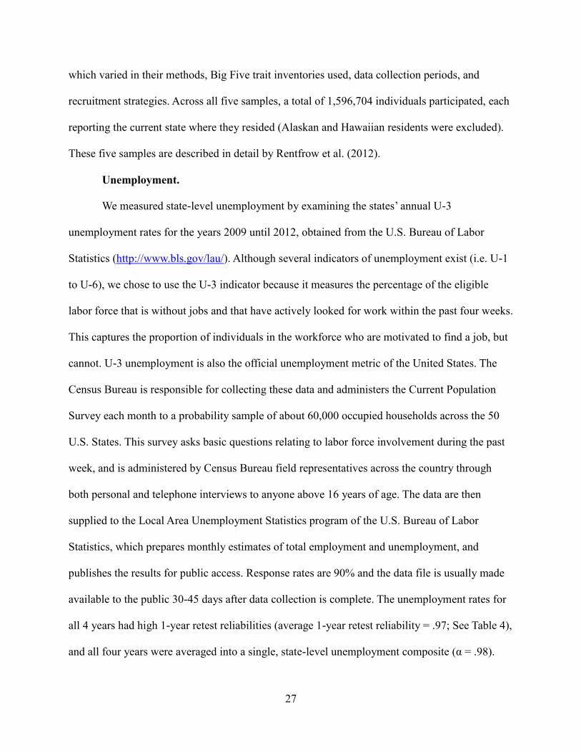
Unemployment.

We measured state-level unemployment by examining the states’ annual U-3

unemployment rates for the years 2009 until 2012, obtained from the U.S. Bureau of Labor

Statistics (http://www.bls.gov/lau/). Although several indicators of unemployment exist (i.e. U-1

to U-6), we chose to use the U-3 indicator because it measures the percentage of the eligible

labor force that is without jobs and that have actively looked for work within the past four weeks.

This captures the proportion of individuals in the workforce who are motivated to find a job, but

cannot. U-3 unemployment is also the official unemployment metric of the United States. The

Census Bureau is responsible for collecting these data and administers the Current Population

Survey each month to a probability sample of about 60,000 occupied households across the 50

U.S. States. This survey asks basic questions relating to labor force involvement during the past

week, and is administered by Census Bureau field representatives across the country through

both personal and telephone interviews to anyone above 16 years of age. The data are then

supplied to the Local Area Unemployment Statistics program of the U.S. Bureau of Labor

Statistics, which prepares monthly estimates of total employment and unemployment, and

publishes the results for public access. Response rates are 90% and the data file is usually made

available to the public 30-45 days after data collection is complete. The unemployment rates for

all 4 years had high 1-year retest reliabilities (average 1-year retest reliability = .97; See Table 4),

and all four years were averaged into a single, state-level unemployment composite (α = .98).

28

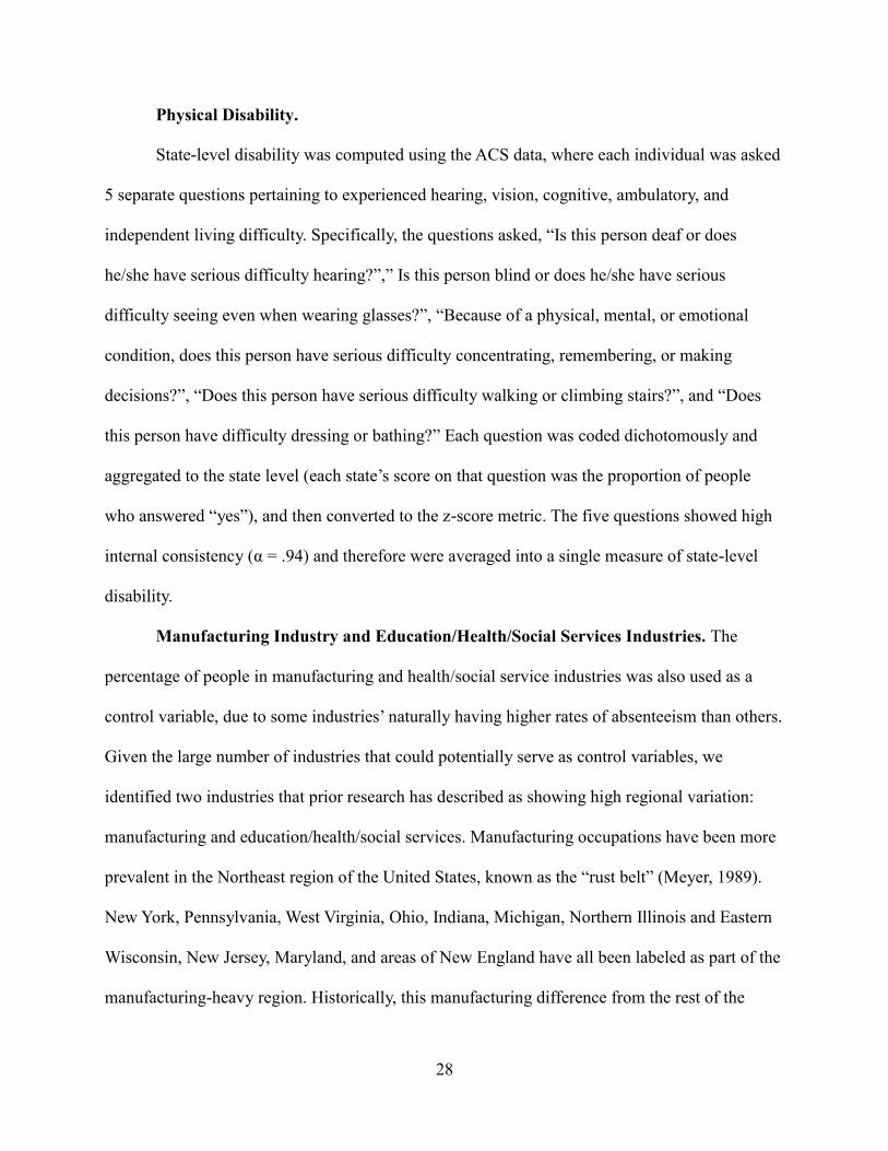
Physical Disability.

State-level disability was computed using the ACS data, where each individual was asked

5 separate questions pertaining to experienced hearing, vision, cognitive, ambulatory, and

independent living difficulty. Specifically, the questions asked, “Is this person deaf or does

he/she have serious difficulty hearing?”,” Is this person blind or does he/she have serious

difficulty seeing even when wearing glasses?”, “Because of a physical, mental, or emotional

condition, does this person have serious difficulty concentrating, remembering, or making

decisions?”, “Does this person have serious difficulty walking or climbing stairs?”, and “Does

this person have difficulty dressing or bathing?” Each question was coded dichotomously and

aggregated to the state level (each state’s score on that question was the proportion of people

who answered “yes”), and then converted to the z-score metric. The five questions showed high

internal consistency (α = .94) and therefore were averaged into a single measure of state-level

disability.

Manufacturing Industry and Education/Health/Social Services Industries. The

percentage of people in manufacturing and health/social service industries was also used as a

control variable, due to some industries’ naturally having higher rates of absenteeism than others.

Given the large number of industries that could potentially serve as control variables, we

identified two industries that prior research has described as showing high regional variation:

manufacturing and education/health/social services. Manufacturing occupations have been more

prevalent in the Northeast region of the United States, known as the “rust belt” (Meyer, 1989).

New York, Pennsylvania, West Virginia, Ohio, Indiana, Michigan, Northern Illinois and Eastern

Wisconsin, New Jersey, Maryland, and areas of New England have all been labeled as part of the

manufacturing-heavy region. Historically, this manufacturing difference from the rest of the

29

country is thought to have arisen from the seaport access where raw materials could arrive, be

processed, and then shipped to the rest of the country through railroad (Kunstler, 1998).

Therefore, because of the manufacturing difference between regions, particularly between the

Western and Eastern parts of the U.S., we would want to control for the absenteeism rates

associated with this industry. Additionally, prior research suggests that Education and Health

related jobs are more prevalent per capita in the Northern part of the U.S., relative to the South

and the West. The point-biserial correlation between Western region and number of teachers per

capita is -.45 (http://nces.ed.gov/programs/stateprofiles/). Additionally, the point-biserial

correlation between Western regions and number of active physicians per capita is -.19 (AAMC,

2011). These data suggest regional differences in manufacturing and education/health services

industries in particular, and therefore these two industry codes would serve as natural candidates

when controlling for industry differences in absenteeism. To get these two industry codes, the

IPUMS provides codes for the industry of a worker using the 15 industry categories in the U.S.

Census: Agriculture, Utilities, Construction, Manufacturing, Wholesale, Retail, Transportation,

Information and Communication, Finance, Professional, Education/Health/Social Services,

Entertainment, Public Administration, Armed Forces, Other. People’s self-reported occupations

were classified by the IPUMS into one of these industries. For each industry, I calculated the

percentage of the workforce within a state who are in that industry.

30

CHAPTER 3

RESULTS

The four main hypotheses of this paper were tested by examining (H1) the correlation

between a state-level social disorganization and absenteeism, (H2) the state-level correlation

between region and social disorganization, (H3) the correlation between a state’s region (West

vs. Non-West) and absenteeism and (H4) whether the association between region and state-level

absenteeism is mediated by social disorganization at the state-level. The first of these hypotheses

suggests that states with higher levels of social disorganization should experience higher rates of

absenteeism. Indeed, the zero-order correlation between the two variables supports this

prediction (r = .67, p < .05; supporting H1; see Table 5 for state-level correlations between all

variables). Hypothesis 2 predicts that, replicating prior research (Baron & Strauss, 1987), states

in the Western region of the United States should be higher in social disorganization. The zero-

order correlation between the two variables is consistent with this prediction (r = .53, p < .05).

Hypothesis 3 predicts that Western states experience greater levels of absenteeism. This

prediction is supported by the point-biserial zero-order correlation between Western region and

absenteeism (r= .49, p<.05). Therefore, the zero-order correlations provide support for the first

three hypotheses that describe the general pattern of associations between a state’s region, social

disorganization, and absenteeism.

To examine the fourth hypothesis, which suggests that the relationship between Western

region and absenteeism can be explained/mediated by that region’s level of social

disorganization, I used both Baron and Kenny’s (1986) regression approach (Table 6) as well as a

test of the indirect effect (bias-corrected bootstrap confidence interval; Preacher & Hayes, 2008;

Hayes & Scharkow, 2013). Regressions are commonly used by researchers to examine: (a) the

31

effect of X on M, and (b) the reduction of the direct effect between X and Y due to including the

proposed mediator (M). As previously discussed in the correlation analysis, the standardized

regression coefficient for the total effect between Western region and social disorganization is β

= .53, p < .05. Further, when social disorganization is included in the model, the coefficient for

Western region predicting Absenteeism falls from β = .49 (p < .05) down to β = .20 (n.s.). This

decrease is consistent with the proposed meditational model, and suggests that the direct effect of

Western region on absenteeism is .20 (n.s.). Including the proposed control variables (state-level

unemployment, disability, extraversion, neuroticism, manufacturing industry,

education/health/social services industry) further decreases the direct effect of Western region on

Absenteeism to β = .08 (n.s.).

To complete the test of mediation, the indirect effect was calculated by multiplying the

coefficient for the path from X to M by the coefficient for the path from M to Y. This product of

coefficients represents the part of the X-Y effect that operates through the mediator. Dividing the

indirect effect by the total effect describes the proportion of the directed effect that is mediated,

and can therefore describe whether the relationship between X and Y is fully (i.e. the proportion

is 1.0) versus partially mediated (i.e., the proportion is less than 1.0) by M.

When conducting a significance test of the indirect effect in mediation, the researcher

must use a sampling distribution for the product, which is often asymmetric. However, there are

various approaches to constructing such a sampling distribution, which may lead to more/less

accurate results. Hayes and Scharkow (2013) compared the performance of various tests of the

mediation indirect effect by simulating a three-variable mediation model with known indirect

effects. Each mediation test was examined for its Type I error rate, Type II error rate, confidence

interval narrowness, and agreement with the other tests. Their results advised against the Sobel

32

test (1982) due its lower power. Rather, they recommended that researchers use bootstrap

confidence intervals when testing mediation. Specifically, when power is a concern, researchers

should use a bias-corrected bootstrapped confidence interval to estimate the variability of the

effect. Simulations found that constructing the sampling distribution of the indirect effect using

bias corrected bootstrapped confidence intervals performs the best at detecting non-zero effects

out of the most common mediation test methods, and can perform well at estimating the true

effect with smaller sample sizes. Due to the limited sample size (i.e., 48 states), power is a

primary concern of testing for mediation here and therefore, the bias corrected bootstrap method

was used to construct confidence intervals for the indirect effect. Because it is a bootstrap

method, it does not assume a sampling distribution when estimating the standard error or

constructing confidence intervals, but rather uses the distribution observed in the dataset.

Therefore, these tests tend to be more robust against deviations from normality.

The mediation model I hypothesized was that the effect of region (West vs. non-West) on

state-level absenteeism is mediated by state-level social disorganization. The indirect effect was

estimated to be .22 (95% bootstrapped CI = [.07, .40]; p < .05). The total effect of region on

absenteeism was .49 (95% bootstrapped CI = [.11, 1.18]; p < .05). Therefore, .22/.49 = 52% of

the total effect of Western region on absenteeism is mediated by social disorganization (Figure

2).

33

CHAPTER 4

REPLICATION OF STATE-LEVEL EFFECTS AT THE

CITY LEVEL

Although social disorganization is a phenomenon that occurs at the regional level, there is

no unanimity from past research on which level-of-analysis (e.g., state, county, city, zip code,

neighborhood, etc.) most naturally corresponds to regional variation in anomie. Although many

arguments could be made for how both state-level and city-level governments, laws, social

histories, and norms systematically differ, it is not obvious which level of analysis is most

theoretically appropriate in the study of absenteeism [cf. Baron & Strauss (1987) posited social

disorganization phenomena at the state level; whereas Shaw & McKay (1942) theorized social

disorganization at the city level]. The current dissertation conceptualized the original hypotheses

at the state-level, primarily because the past research that has implicated regional geographic

differences in social disorganization (Baron & Strauss, 1987; 1989) also used states. The benefit

of having past research to draw upon is that using states allows parts of the current dissertation to

be cross-validated against the previous findings that also used states. Therefore, some aspects of

the current research such as the state-level measure of social disorganization, and the relationship

between Western region and social disorganization, can be checked for consistency against

previous measures and findings. Additionally, when aggregating the absenteeism response up to

higher levels, the measure showed the highest amount of the year-to-year reliability at the state-

level, suggesting that the aggregated scores are most likely to be stable across time—and the

effects are least likely to be attenuated—at the state level of analysis.

Despite the advantages conferred by examining the main variables at the state-level, there

are nonetheless certain disadvantages to using states compared to using other regional levels that

34

have also been studied in social disorganization research. State-level analyses ignore within-state

variation. Thus, people in a politically/geographically/demographically diverse state (e.g., Texas)

will experience varying levels of disorganization (i.e., some regions are high and some are low)

in their daily life, and the state average will not necessarily reflect the typical experience or

social pressures encountered by its residents in more local communities.

As discussed, the state level is not the only level at which social disorganization pressures

can exist, and in fact much social disorganization research has relied on using smaller regions

such as cities, zip codes, or metropolitan areas. That is, when a community experiences

conditions that undermine the ability for its residents to enact social control, the community also

tends to exhibit higher levels of deviant behavior (see Introduction, for a review). Thus, although

the hypotheses were originally conceptualized at the state-level, the underlying theory has also

been applied to lower levels. Because the effect of social disorganization is commonly discussed

as also occurring at the city level and zip code level, examining the current hypotheses in smaller

regions provides another opportunity to test the proposed relationships in ways that can address

some of the methodological disadvantages encountered by using states. One of the major

advantages of analyzing a lower level, such as a city, is that the scores obtained from a city

provide a much more nuanced view of a region. According to Tobler’s “First Law of Geography”

(1970), which states that nearby things are more similar than distant things, responses coming

from a concentrated area in a city should show more homogeneity than responses that come from

different, spread-out areas in a state. As such, the social disorganization index value assigned to

Chicago, for example, could be more representative of that region (i.e., contain less within-

region variability) than the social disorganization index of the entire state of Illinois. A second,

and perhaps more important, advantage of city-level analysis is that using states to study the

35

effects of social disorganization and absenteeism will limit the available sample size (e.g., 48

continental United States), crippling statistical power.

Due to the disadvantages encountered from examining states, and the potential

advantages of examining social disorganization at lower, more local levels, I attempted to

replicate the findings found at the state-level, using analyses at the Metropolitan Statistical Area

(MSA) level. The ACS questionnaire asks participants to report the city of their occupation, and

this allows many of the key variables to be constructed at the city level of analysis.

Method

For the city-level analyses, I attempted to use the same data sources as those used in the

state-level analyses that are the focus of this dissertation. The city-level analyses are based upon

N = 292 Metropolitan Statistical Areas (MSAs), which we simply refer to as “cities”. To examine

the city-level associations among region (West vs. non-West), social disorganization, and

absenteeism; the same variables previously computed at the state-level were recreated for each

city. However, city-level geographic status is only reported for the years 2009-2011 in the ACS

dataset, and therefore only three years are available for aggregation to the city level. In the ACS

data, participants were asked to identify the metropolitan area of their occupation. This

metropolitan area of occupation was then used as the grouping variable for computing the city-

level means of the other variables in the analyses. Specifically, the variables used were

geographic region, absenteeism, social disorganization (same indicator variables as those used in

the state-level analyses, with the exception of irreligiosity, which is not available at the city

level), disability (same indicator variables as those used in the state-level analyses),

unemployment, and industry of occupation. Each city’s region (West vs. Non-West) was coded

36

dichotomously by whether the city was located in a Western (coded as a 1) versus non-Western

(coded as a 0) state (NWest = 51, Nnon-West = 241).

Results

Similar to state-level absenteeism, city-level absenteeism showed high re-test reliability

from year to year (average r = .85; as reported in the Method section, Table 1), and I therefore

averaged it into a single composite measure of city-level absenteeism for the years 2009 to 2011

(see Figure 3 for a depiction of city-level absenteeism rates). To construct the social

disorganization index at the city-level, all the subfacets present at the city-level in the ACS data

were used (i.e., moved home, moved state, single, divorced, and single female head of

household), whereas the one subfacet not recorded in the IPUMS data (i.e. irreligiosity) could

not be included in the social disorganization index. Prior to creating the composite index, I

standardized all items at the city level by transforming them into z-scores. As with the state-level

social disorganization items, the proportion of single mothers with children did not correlate

highly with the other items (item-total correlation = .13), and was thus dropped from the social

disorganization scale (the same as was done at the state level). The remaining scale showed city-

level internal consistency of α = .62, which is slightly lower than the α = .67 reliability found at

the state level; this is likely due to the fact that the city-level social disorganization scale has only

4 items, as opposed to the 5-item measure used at the state level (i.e., irreligiousity scores were

not available at the city level). Indeed, by applying the Spearman-Brown prophecy formula to the

scale, the city-level reliability would increase to .67 if another parallel item were added, which is

the same as the reliability obtained at the state-level. For each city, these 4 items were then

averaged into a single index of social disorganization (see Table 7 for city-level social

disorganization index scores).

37

I recreated the control variables that could be computed from the ACS data or from

publically available information during the period covered by the ACS in which they reported the

metropolitan area of each respondent’s occupation (i.e., from 2009-2011). These included city-

level unemployment, city-level disability, and city-level industries. The only regional variables

that could not be recreated at the city level were the Big Five personality variables. City-level

unemployment was obtained from the U.S. Bureau of Labor Statistics, which provides the

average U-3 unemployment rate for each metropolitan statistical area for a given year (i.e., for

2009, 2010, and 2011). Unemployment rates showed high retest reliability (average r = .97), and

were averaged into a single index of city-level unemployment. City-level disability was

computed in the same manner as at the state level (city-level α = .88) (see Table 8 for correlation

matrix among all variables).

I re-examined the four state-level hypotheses that were previously made (but this time, at

the city level), using the same steps described in the previous section. Hypothesis 1 was

supported at the city level (social disorganization positively relates to absenteeism; r = .35, p <

.05). The second hypothesis was also supported at the city level (cities in the Western region of

the U.S. were higher in social disorganization; r = .19, p < .05). Hypothesis 3 predicts that

Western cities experience greater levels of absenteeism, and was also supported (r= .22, p<.05).

Therefore, the zero-order correlations at the city level supported the first three hypotheses, and

were consistent with the findings at the state-level of analysis.

To examine the fourth hypothesis, which specifies that the relationship between Western

region and absenteeism can be explained by that region’s level of social disorganization, I used

both a regression approach (Table 9) as well as a more specific mediation analysis of the indirect

effect. The standardized regression coefficient for the total effect between Western region and

38

social disorganization is β = .19 (p < .05). Further, when social disorganization is included in the

model, the coefficient for Western region predicting Absenteeism decreases from β = .22 (p <

.05) to β = .15 (p < .05). Including the proposed control variables (city-level unemployment,

disability, manufacturing industry, and education/health/social services industry) yields a similar

direct effect of Western region on Absenteeism of β = .17 (p < .05). For the city-level mediation

analysis, the indirect effect was estimated to be .06 (95% CI = [.03, .11]; p < .05). The total effect

of region on absenteeism was .22, and therefore .06/.22 = 28%, of the total effect of Western

region on absenteeism is mediated, at the city level of analysis (Figure 4). In sum, all of the

hypothesized effects found at the state level of analysis were also supported at the city level of

analysis, in terms of both the directions of the effects and the statistical significance tests for the

effects.

39

CHAPTER 5

DISCUSSION

The state-level hypotheses made in the introduction were all supported. States with

higher levels of social disorganization experienced higher levels of absenteeism. This state-level

social disorganization was higher in the Western region of the United States, which replicated the

findings of past research (Baron & Strauss, 1987). Additionally, this project found evidence that

Western states tend to experience higher levels of absenteeism. This effect of heightened Western

regional state-level absenteeism was explained/mediated by state-level social disorganization.

The current project offers many novel insights that have implications for research pertaining to

both social disorganization and group-level absenteeism.

Whereas prior research on social disorganization has primarily focused on explaining

violent deviant behavior (e.g., rape, homicide, and assault), the current research demonstrates

that social disorganization is associated with a non-violent form of deviant behavior: work

absenteeism. This relationship between social disorganization and absenteeism, however, is

consistent with the underlying process suggested by social disorganization theory, where

disorganization enables anti-social behaviors that would otherwise be deterred by public

vigilance, family socialization, and a collectivist mindset (see Introduction for further

elaboration). Therefore, future conceptualizations of social disorganization may prefer to use

broader terms when describing the types of behaviors that can be affected by weakened social

control.

This research also represents one of the first examinations of absenteeism at the

geographic (i.e., state) level. Although group-level absenteeism has been studied at the team- or

office-level by other researchers, few (if any) have conceptualized it at the level of an entire state

40

or city. In the present study, state-level absenteeism showed high retest-reliability (r = .96),

which provides some evidence that it reflects a stable construct that has the potential to be

predicted by other variables. As such, absenteeism may exist at higher levels than those

previously explored in the group-absenteeism literature, and this higher level may not share the

same predictors/precursors as absenteeism at a lower group-level. Thus, state-level absenteeism

phenomena may provide new theoretical opportunities for researchers studying group-level

absence.

Further, the current research not only suggests that states exhibit a consistent rank-order

of absenteeism over time, but that this state-level variation can be explained by structural factors

specific to those states. Specifically, this project highlights the role of social disorganization

(e.g., family stability, residential mobility, irreligiosity) as one explanation. This work therefore

contributes to psychological understanding of regional differences, particularly in the Western

U.S. The findings suggest that there exist regional cultures of absence, where Western states tend

to experience higher rates of absenteeism compared to non-Western states. The difference in

these regional cultures of absence can be partially accounted for by the social disorganization of

the region. This novel regional difference adds to the body of psychological research that has

examines the unique characteristics of Western regions. Some prior research finds that the

Western region (compared to the Northern and Southern regions) is more likely to endorse

statements of legitimate violence, and to support retribution (Baron & Strauss, 1987; Cohen,

1996). Research examining state-level personality differences finds that Western states are

particularly low on neuroticism and extraversion—a temperament the researchers refer to as

“relaxed and creative” (Rentfrow, Gosling, Jokela, Stillwell, Kosinski, & Potter, 2012). The

41

current work supplements those prior findings by implicating an additional region difference—

absenteeism.

It is also important to address the limitations of the current research. Caution must be

taken when making claims about any causal effect that living in a Western region has on social

disorganization and absenteeism. All three variables were measured cross-sectionally, and

therefore no temporal precedence of one variable over another (i.e., X occurred before Y) can be

assumed. One explanation for the pattern of correlations observed in this project is that states

with higher rates of social disorganization may have less ability to enact social control, thereby

leading to reduced normative pressure on absence. This explanation is consistent with how prior

social disorganization research conceptualizes the process. However, an alternative explanation

could be that people with poor work attendance are more likely to congregate in regions (i.e., the

West) that have occupations more tolerant of absenteeism. This migration/gravitational

explanation requires Western state residents to have a high rate of mobility and a loose family

structure, which could lead to greater observed social disorganization in those regions. However,

nearly all social disorganization research suffers from this limitation, because social

disorganization is typically measured based on archival datasets, and it is difficult if not

impossible for researchers to randomly assign communities to be more socially disorganized than

others. Therefore the current findings are meant to be interpreted only as correlational, and

consistent with the pattern one would expect according to the common social disorganization

process model.

Another limitation is the lack of information available at the state-level. That is, this

project could only include variables that were measured by the IPUMS or that have been

previously aggregated to the state-level within the timeframe of the study. Therefore, there could

42

be theoretically relevant variables that past research suggests influence absenteeism (e.g., job

satisfaction), but which could not be included in the current study as control variables. Given that

this project is one of the first to examine absenteeism at the state-level of analysis, there was no

clear indication of what variables should be included in the model (i.e., because homologous

bivariate relationships between the individual and state-level cannot be assumed). Therefore

future research that has different datasets, and a different selection of variables, may wish to

examine how robust the findings are when other covariates and explanatory mechanisms are

included.

An additional limitation of the study is the measure that was used to index absence. The

absenteeism measure was taken directly from the ACS, which asked about a person’s absence

only during the prior week. This short observation window will lead to greater unreliability,

because of the low base rate of absences during a single week. Because of this anticipated

unreliability, I aggregated up to the state level and across years to form a more reliable measure.

However, because the average year-to-year retest correlation of absenteeism at the individual

level is only r = .00, aggregating across 3 or 4 years would not be expected to increase the

reliability of the individual-level absence measure to an acceptable level. This low reliability

would have greatly attenuated the observed effect sizes/correlations between variables, and

therefore prohibits examining hypotheses involving individual-level absence, including cross-

level relationships. Further, the individual-level measure of absence was self-reported. Self-

reported measures may suffer from measurement error due to forgetting, and may be biased due

to self-presentation and norms (Harrison & Shaffer, 1994). Whereas the short retrospective

window minimizes measurement error which might have been due to people not remembering

whether they were absent during the past week, the results could potentially be biased.

43

Respondents may underreport their actual absence to preserve their public image. If there are

regional differences in people’s social desirability biases, such as absence norms, then it is

possible that the differing absence rates across regions are the result of respondents’ selectively

reporting better absences in locations where the residents view absenteeism as more deviant.

This possibility may be minimized by the anonymity of the questionnaire, the legal repercussions

one could face by falsifying information, and the lack of ambiguity of the question (i.e., absence

was defined as missing work for any non-dismissal related reason).

These results provide some direction for future research. One question that could be

further explored is whether other related deviant behaviors at the regional level can also be

explained by the social disorganization in a region. Specifically, absenteeism is sometimes

treated as a subfacet of a broader category of deviant behaviors referred to as “counterproductive

work behavior” (CWB; Robinson & Bennett, 1995; Sackett, 2002). This category groups

together employee behaviors that go against the legitimate interests of an organization. Some

examples of CWBs include destruction of property, theft, gossiping, harassment of other

employees, intentionally working slowly, poor quality of work, among others (Robinson &

Bennett, 1995; Gruys & Sackett, 2003). Future research may choose to examine whether there

are regional cultures not only of absence, but of other CWBs.

In summary, the current project found support for the central hypotheses that predicted an

association between Western regions of the United States, regional rates of social

disorganization, and rates of absenteeism in those regions. Additionally, results provided

evidence that the association between Western region and absenteeism at the state-level is

mediated by the amount of social disorganization in the region. This research attempts to

44

integrate ideas from multiple disciplines in a novel way that provides insight into a traditionally

individual-level outcome, using a cultural/sociological perspective.

45

REFERENCES

American Association of Medical Colleges (2011, November). 2011 State Physician Workforce

Data Book. Retrieved October 2014, from

https://www.aamc.org/download/263512/data/statedata2011.pdf

Bachman, R. (1991). An analysis of American Indian homicide: A Test of social disorganization

and economic deprivation at the reservation county level. Journal of Research in Crime

and Delinquency, 28, 456–471.

Bainbridge, W. S. (1990). Explaining the church member rate. Social Forces, 68, 1287–1296.

Barham, C., & Leonard, J. (2002). Trends and sources of data on sickness absence. Labour

Market Trends, 110, 177–185.

Baron, L., & Straus, M. A. (1987). Four Theories of Rape: A macrosociological analysis. Social

Problems, 34, 467–489.

Baron, L., & Straus, M. A. (1989). Four theories of rape in American society: A state-level

analysis. Yale University Press.

Baron, R. M., & Kenny, D. A. (1986). The moderator–mediator variable distinction in social

psychological research: Conceptual, strategic, and statistical considerations. Journal of

Personality and Social Psychology, 51, 1173.

Baumer, E. P. (2002). Neighborhood disadvantage and police notification by victims of

violence. Criminology, 40, 579–616.

Bellair, P. E., & Browning, C. R. (2010). Contemporary disorganization research: An

assessment and further test of the systemic model of neighborhood crime. Journal of

Research in Crime and Delinquency, 47, 496–521.

46

Bering, J. M., & Johnson, D. D. (2005). “O Lord You Perceive my Thoughts from Afar”:

Recursiveness and the evolution of supernatural agency. Journal of Cognition and Culture,

5, 1–2.

Berry, C. M., Lelchook, A. M., & Clark, M. A. (2012). A meta-analysis of the interrelationships

between employee lateness, absenteeism, and turnover: Implications for models of

withdrawal behavior: Withdrawal Behaviors: A meta-analysis. Journal of Organizational

Behavior, 33, 678–699.

Blau, J. R., & Blau, P. M. (1982). The cost of inequality: Metropolitan structure and violent

crime. American Sociological Review, 114–129.

Blau, P. M. (1964). Exchange and power in social life. New York: J. Wiley.

Blau, P. M., & Golden, R. M. (1986). Metropolitan structure and criminal violence. The

Sociological Quarterly, 27, 15–26.

Bouffard, L. A., & Muftic, L. R. (2006). The “rural mystique”: Social disorganization and

violence beyond urban communities. Western Criminology Review, 7, 56–66.

Braga, A. A., & Clarke, R. V. (2014). Explaining high-risk concentrations of crime in the city:

Social disorganization, crime opportunities, and important next steps. Journal of Research

in Crime and Delinquency, 51, 480–498.

Burgess, E. W., McKenzie, R. D., Park, R. E., & others. (1967). The city. Chicago: University of

Chicago Press.

Bursik Jr, R. J., & Grasmick, H. G. (1993). Economic deprivation and neighborhood crime rates,

1960-1980. Law & Society Rev., 27, 263.

47

CCH Incoporated. (2006, October). Unscheduled absences rising at U.S. workplaces. Retrieved

July 2014, from http://www.agi.com/downloads/media-center/in-the-news/HRMN_641-

06_PIN.pdf

Chadwick-Jones, J. K., Nicholson, N., & Brown, C. (1982). Social psychology of absenteeism.

Praeger New York.

Chan, D. (1998). Functional relations among constructs in the same content domain at different

levels of analysis: A typology of composition models. Journal of Applied Psychology, 83,

234.

Cohen, D. (1996). Law, social policy, and violence: The impact of regional cultures. Journal of

Personality and Social Psychology, 70, 961.

Cohen, D. (1998). Culture, social organization, and patterns of violence. Journal of Personality

and Social Psychology, 75, 408.

Cohen, D., & Nisbett, R. E. (1994). Self-protection and the culture of honor: Explaining

southern violence. Personality and Social Psychology Bulletin, 20, 551–567.

Cohen, D., & Nisbett, R. E. (1997). Field experiments examining the culture of honor: The Role

of Institutions in Perpetuating Norms about Violence. Personality and Social Psychology

Bulletin, 23, 1188–1199.

Cooke, L. N. (2013). Religious establishments, public housing, and liquor stores: Their

prediction of juvenile system behavior. (Unpublished doctoral dissertation). City University

of New York.

Cropanzano, R. (2005). Social Exchange Theory: An Interdisciplinary Review. Journal of

Management, 31, 874–900.

48

Crutchfield, R. D., Geerken, M. R., & Gove, W. R. (1982a). Crime rate and social integration

The impact of metropolitan mobility. Criminology, 20, 467–478.

Crutchfield, R. D., Geerken, M. R., & Gove, W. R. (1982b). Crime Rate and Social Integration

The Impact of Metropolitan Mobility. Criminology, 20, 467–478.

Diestel, S., & Schmidt, K.-H. (2010). Interactive effects of emotional dissonance and self-

control demands on burnout, anxiety, and absenteeism. Journal of Vocational Behavior, 77,

412–424.

Durkheim, É. (1933). The Division of Labor in Society. Free Press.

Elshtain, J. B. (1996). Democracy on trial. New York: Basic Books.

Epstein, S. (1979). The stability of behavior: I. On predicting most of the people much of the

time. Journal of Personality and Social Psychology, 37, 1097.

Epstein, S. (1980). The stability of behavior: II. Implications for psychological research.

American Psychologist, 35, 790.

Evans, T. D., Cullen, F. T., Dunaway, R. G., & Burton, V. S. (1995). Religion and crime

reexamined: The impact of religion, secular controls, and social ecology on adult

criminality. Criminology, 33, 195–224.

Gellatly, I. R. (1995). Individual and group determinants of employee absenteeism: Test of a

causal model. Journal of Organizational Behavior, 16, 469–485.

George, J. M., & James, L. R. (1993). Personality, affect, and behavior in groups revisited:

Comment on aggregation, levels of analysis, and a recent application of within and between

analysis.

Gouldner, A. W. (1960). The norm of reciprocity: A preliminary statement. American

Sociological Review, 161–178.

49

Gruys, M. L., & Sackett, P. R. (2003). Investigating the dimensionality of counterproductive

work behavior. International Journal of Selection and Assessment, 11, 30–42.

Hacket, R. D. (1989). Work attitudes and employee absenteeism: A synthesis of the literature*.

Journal of Occupational Psychology, 62, 235–248.

Hammer, T. H., & Landau, J. C. (1981). Methodological issues in the use of absence data.

Journal of Applied Psychology, 66, 574.

Hanisch, K. A., & Hulin, C. L. (1990). Job attitudes and organizational withdrawal: An

examination of retirement and other voluntary withdrawal behaviors. Journal of Vocational

Behavior, 37, 60–78.

Hanisch, K. A., & Hulin, C. L. (1991). General attitudes and organizational withdrawal: An

evaluation of a causal model. Journal of Vocational Behavior, 39, 110–128.

Hanisch, K. A., Hulin, C. L., & Roznowski, M. (1998). The importance of individuals’

repertoires of behaviors: The scientific appropriateness of studying multiple behaviors and

general attitudes. Journal of Organizational Behavior, 19, 463–480.

Harrison, D. A., Newman, D. A., & Roth, P. L. (2006). How important are job attitudes? Meta-

analytic comparisons of integrative behavioral outcomes and time sequences. Academy of

Management Journal, 49, 305–325.

Harrison, D. A., & Shaffer, M. A. (1994). Comparative examinations of self-reports and

perceived absenteeism norms: Wading through Lake Wobegon. Journal of Applied

Psychology, 79, 240.

Hausknecht, J. P., Hiller, N. J., & Vance, R. J. (2008). Work-unit absenteeism: Effects of

satisfaction, commitment, labor market conditions, and time. Academy of Management

Journal, 51, 1223–1245.

50

Hayes, A. F., & Scharkow, M. (2013). The relative trustworthiness of inferential tests of the

indirect effect in statistical mediation analysis: Does method really matter? Psychological

Science, 24, 1918–1927.

Herman, J. B. (1973). Are situational contingencies limiting job attitude-job performance

relationships? Organizational Behavior and Human Performance, 10, 208-224.

Hill, J. M. M. (1955). Changes in accidents and other absences with length of service: A further

study of their incidence and relation to each other in an iron and steel works. Human

Relations, 8, 121–152.

Hulin, C.L. (1991). Adaptation, persistence, and commitment in organizations. In Dunnette,

M.D. & Hough, L.M. (Eds.), Handbook of industrial and organizational psychology (2nd

ed., Vol. 2, pp. 445–505). Palo Alto, CA: Consulting Psychologists Press.

Hutchison, S., Sowa, D., Eisenberger, R., & Huntington, R. (1986). Perceived organizational

support. Journal of Applied Psychology, 71, 500–507.

James, L. R., Demaree, R. G., & Wolf, G. (1984). Estimating within-group interrater reliability

with and without response bias. Journal of Applied Psychology, 69, 85.

James, L. R., Demaree, R. G., & Wolf, G. (1993). rwg: An assessment of within-group interrater

agreement. Journal of Applied Psychology, 78, 306.

Johns, G. (1997). Contemporary research on absence from work: Correlates, causes and

consequences. International Review of Industrial and Organizational Psychology, 12, 115–

174.

Johnson, D., & Bering, J. (2009). Hand of God, mind of man. The Believing Primate: Scientific,

Philosophical, and Theological Reflections on the Origin of Religion, 26–44.

51

Kasarda, J. D., & Janowitz, M. (1974). Community attachment in mass Society. American

Sociological Review, 39, 328.

Knox, J. B. (1961). Absenteeism and turnover in an Argentine factory. American Sociological

Review, 424–428.

Komhauser, W. (1946). The Politics of Mass Society. Cf. Duncan MacRae, Jr., Parliament,

Parties and Society in France, 1958, 28–32.

Kosmin, B. A., & Keysar, A. (2008). Unitarian-Universalists in the United States 1990-2008:

Socio-demographic Trends and Religious Patterns. Retrieved from

http://digitalrepository.trincoll.edu/cgi/viewcontent.cgi?article=1061&context=facpub

Kozlowski, S. W., & Klein, K. J. (2000). A multilevel approach to theory and research in

organizations: Contextual, temporal, and emergent processes.

Kronos Incorporated. (2010, June). Total Financial Impact of Employee Absences in the U.S.

Retrieved July 2014, from http://www.kronos.com/pr/unplanned-absence-costs-

organizations-over-8-percent-of-payroll.aspx

Kronos Incorporated. (2014, August). Total Financial Impact of Employee Absences in the U.S.

Retrieved July 2014, from http://www.shrm.org/research/surveyfindings/documents/14-

0531%20exsummary_impactabsence_final.pdf

Kubrin, C. E., & Weitzer, R. (2003). New directions in social disorganization theory. Journal of

Research in Crime and Delinquency, 40, 374–402.

Kunstler, J. H. (1998). Home from nowhere: remaking our everyday world for the twenty-first

Century. New York: Simon & Schuster.

March, J., & Simon, H. (1993). Organizations. Cambridge, Mass., USA: Blackwell.

52

Markham, S. E., & McKee, G. H. (1995). Group absence behavior and standards: A multilevel

analysis. Academy of Management Journal, 38, 1174–1190.

Martin , J. (1971). Some aspects of absence in a light engineering factory. Occupational

Psychology, 45, 77-89.

Martocchio, J. J. (1992). The financial cost of absence decisions. Journal of Management, 18,

133–152.

Martocchio, J. J. (1994). The effects of absence culture on individual absence. Human Relations,

47, 243–262.

Martocchio, J. J., Harrison, D. A., & Berkson, H. (2000). Connections between lower back pain,

interventions, and absence from work: A time-based meta-analysis. Personnel Psychology,

53, 595–624.

McShane, S. L. (1984). Job satisfaction and absenteeism. Canadian Journal of Administrative

Sciences/Revue Canadienne Des Sciences de l’Administration, 1, 61–77.

Meyer, D. R. (1989). Midwestern industrialization and the American manufacturing belt in the

nineteenth century. The Journal of Economic History, 49, 921.

Mitra, A., Jenkins, G. D., & Gupta, N. (1992). A meta-analytic review of the relationship

between absence and turnover. Journal of Applied Psychology, 77, 879.

Morgeson, F. P., & Hofmann, D. A. (1999). The structure and function of collective constructs:

Implications for multilevel research and theory development. Academy of Management

Review, 24, 249–265.

Nicholson, N. (1975). Industrial absence as an indicant of employee motivation and job

satisfaction. Unpublished doctoral thesis. University of Wales, Cardiff

53

Nicholson, N., & Johns, G. (1985). The Absence culture and the Poychological Contract-Who’s

in control of absence? The Academy of Management Review, 10, 397.

Nisbett, R. E., & Cohen, D. (1996). Culture of honor: The psychology of violence in the South.

Westview Press.

Oishi, S. (2010). The psychology of residential mobility implications for the self, social

relationships, and well-being. Perspectives on Psychological Science, 5, 5–21.

Oishi, S., Lun, J., & Sherman, G. D. (2007). Residential mobility, self-concept, and positive

affect in social interactions. Journal of Personality and Social Psychology, 93, 131.

Ostroff, C. (1993). The effects of climate and personal influences on individual behavior and

attitudes in organizations. Organizational Behavior and Human Decision Processes, 56,

56–90.

Park, R. E., Burgess, E. W., & Janowitz, M. (1921). Introduction to the Science of Sociology.

University of Chicago Press Chicago.

Petee, T. A., & Kowalski, G. S. (1993). Modeling rural violent crime rates: A test of social

disorganization theory. Sociological Focus, 26, 87–89.

Pettersson, T. (1991). Religion and criminality: Structural relationships between church

involvement and crime rates in contemporary Sweden. Journal for the Scientific Study of

Religion, 279–291.

Pfohl, S. (1985). Toward a sociological deconstruction of social problems. Social Problems,

228–232.

Rauch, J. (1996, May 6). For better or worse. New Republic, pp. 18-23.

54

Preacher, K. J., & Hayes, A. F. (2008). Asymptotic and resampling strategies for assessing and

comparing indirect effects in multiple mediator models. Behavior Research Methods, 40,

879–891.

Rentfrow, P. J. (2010). Statewide differences in personality: Toward a psychological geography

of the United States. American Psychologist, 65, 548–558.

Rentfrow, P. J., Gosling, S. D., Jokela, M., Stillwell, D. J., Kosinski, M., & Potter, J. (2013).

Divided we stand: Three psychological regions of the United States and their political,

economic, social, and health correlates.

Rhodes, S. R., & Steers, R. M. (1990). Managing employee absenteeism. Addison-Wesley

Reading, MA.

Roberts, K. H., Hulin, C. L., & Rousseau, D. M. (1978). Developing an interdisciplinary science

of organizations. San Francisco: Jossey-Bass.

Robinson, W. (1950). Ecological Correlations and the Behavior of Individuals. American

Sociological Review, 15, 351–357.

Robinson, S. L., & Bennett, R. J. (1995). A typology of deviant workplace behaviors: A

multidimensional scaling study. Academy of Management Journal, 38, 555–572.

Rose, D. R. (2000). Social disorganization and parochial control: Religious institutions and their

communities. In Sociological Forum (Vol. 15, pp. 339–358). Springer.

Rosse, J. G., & Miller, H. E. (1984). Relationship between absenteeism and other employee

behaviors. Absenteeism, 1, 194–228.

Ruggles, S., & Alexander, J. T., Genadek, K., Goeken, R., Schroeder, M.B., & Sobek, M.

(2010). Integrated Public Use Microdata Series: Version 5.0.

55

Salgado, J. F. (2002). The Big Five personality dimensions and counterproductive behaviors.

International Journal of Selection and Assessment, 10, 117–125.

Sampson, R. J. (1991). Linking the micro-and macrolevel dimensions of community social

organization. Social Forces, 70, 43–64.

Sampson, R. J. (1997). The Embeddedness of Child and Adolescent Development. In J. McCord

(Ed.), Violence and Childhood in the Inner City (pp. 31–77). Cambridge: Cambridge

University Press. Retrieved from http://dx.doi.org/10.1017/CBO9780511571015

Sampson, R. J., & Bartusch, D. J. (1998). Legal cynicism and (subcultural?) tolerance of

deviance: The neighborhood context of racial differences. Law and Society Review, 777–

804.

Sampson, R. J., & Groves, W. B. (1989). Community structure and crime: Testing social-

disorganization theory. American Journal of Sociology, 774–802.

Sampson, R. J., Raudenbush, S. W., & Earls, F. (1997). Neighborhoods and violent crime: A

multilevel study of collective efficacy. Science, 277, 918–924.

Schaufeli, W. B., Bakker, A. B., & Van Rhenen, W. (2009). How changes in job demands and

resources predict burnout, work engagement, and sickness absenteeism. Journal of

Organizational Behavior, 30, 893–917.

Scott, K. D., & Taylor, G. S. (1985). An examination of conflicting findings on the relationship

between job satisfaction and absenteeism: A meta-analysis. Academy of Management

Journal, 28, 599–612.

Shaw, C. R., & McKay, H. D. (1942). Juvenile delinquency and urban areas. Chicago, Ill.

Simpson, M. E. (1985). Violent crime, income inequality, and regional culture: Another look.

Sociological Focus, 199–208.

56

Smith, F. J. (1977). Work attitudes as predictors of attendance on a specific day. Journal of

Applied Psychology, 62, 16-19.

Sobel, M. E. (1982). Asymptotic confidence intervals for indirect effects in structural equation

models. Sociological Methodology, 13(1982), 290–312.

Stark, R., & Bainbridge, W. S. (1985). The future of religion: secularization, revival, and cult

formation. Berkeley: University of California Press.

Steers, R. M., & Rhodes, S. R. (1978). Major influences on employee attendance: A process

model. Journal of Applied Psychology, 63, 391.

Stewart, W. F., Ricci, J. A., Chee, E., Hahn, S. R., & Morganstein, D. (2003). Cost of lost

productive work time among US workers with depression. Journal of the American

Medical Association, 289, 3135–3144.

Stockford, L. (1944). Chronic absenteeism and good attendance. Personnel Journal, 23, 202–

207.

Swider, B. W., & Zimmerman, R. D. (2010). Born to burnout: A meta-analytic path model of

personality, job burnout, and work outcomes. Journal of Vocational Behavior, 76, 487–

506.

Terborg, J. R. Organizational climate and organizational performance: An empirical

investigation of key issues. Paper presented at the 42nd Annual Meeting of the Academy of

Management, New York 1982.

Theodori, G. L. (2004). Exploring the association between length of residence and community

attachment: A research note. Southern Rural Sociology, 20, 107–122.

Thibaut, J. W. (1986). The social psychology of groups. New Brunswick, U.S.A: Transaction

Books.

57

Thorndike, E. L. (1939). On the fallacy of imputing the correlations found for groups to the

individuals or smaller groups composing them. The American Journal of Psychology, 122–

124.

Tobler, W. R. (1970). A computer movie simulating urban growth in the Detroit region.

Economic Geography, 46, 234–240.

Williams, K. R., & Flewelling, R. L. (1988). The social production of criminal homicide: A

comparative study of disaggregated Rates in American Cities. American Sociological

Review, 53, 421.

Wolfgang, M. E., Ferracuti, F., & Mannheim, H. (1967). The subculture of violence: Towards

an integrated theory in criminology (Vol. 16). Tavistock Publications London.

Wortham, S. E. F. (2006). Learning identity: The joint emergence of social identification and

academic learning. Cambridge University Press Cambridge.

Yu, J., & Newman, D. A. (August, 2006). Social influence and absenteeism: Norms, networks,

and the role of guilt. In T. R. Lituchy (Chair), Predicting Withdrawal: Turnover Intentions

and Absenteeism. Symposium presented at the 66th annual meeting of the Academy of

Management, Atlanta, GA.

58

FIGURES AND TABLES

Figure 1: Map of Absenteeism rates at the State-level

Note: Absenteeism rates were z-scored prior to plotting. Darker colors signify higher

absenteeism rates.

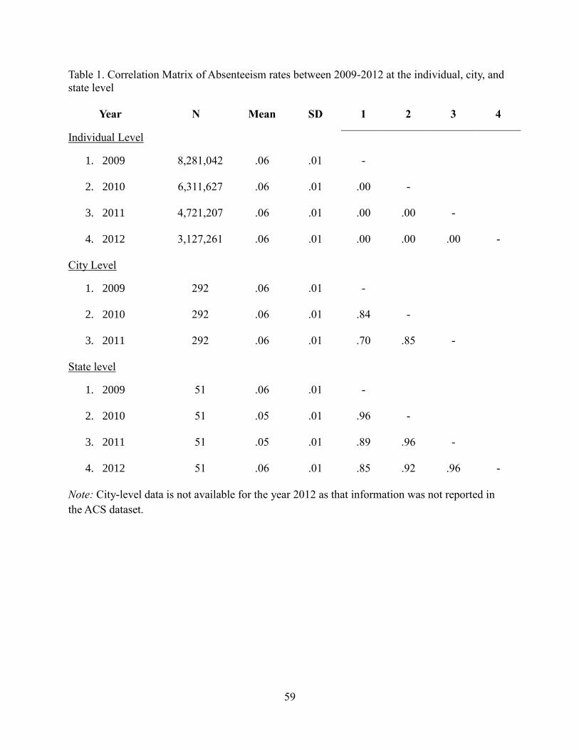
59

Table 1. Correlation Matrix of Absenteeism rates between 2009-2012 at the individual, city, and

state level

Year N Mean SD 1 2 3 4

Individual Level

1. 2009

8,281,042 .06 .01 -

2. 2010

6,311,627 .06 .01 .00 -

3. 2011

4,721,207 .06 .01 .00 .00 -

4. 2012

3,127,261 .06 .01 .00 .00 .00 -

City Level

1. 2009

292 .06 .01 -

2. 2010

292 .06 .01 .84 -

3. 2011

292 .06 .01 .70 .85 -

State level

1. 2009

51 .06 .01 -

2. 2010

51 .05 .01 .96 -

3. 2011

51 .05 .01 .89 .96 -

4. 2012

51 .06 .01 .85 .92 .96 -

Note: City-level data is not available for the year 2012 as that information was not reported in

the ACS dataset.

60

Table 2. Correlation Matrix of State-Level Social Disorganization Index Indicators

Indicator Mean SD 1 2 3 4 5 6

1. Divorce

.11 .01 -

2. Single with

Children

.05 .01 .46 -

3. Irreligious

.16 .06 .21 -.39 -

4. Living Alone

.24 .06 .02 -.27 .45 -

5. Moved House .15 .03 .32 -.12 .15 .33 -

6. Moved State .03 .01 -.01 -.18 .29 .57 .54 -

Note: State-level data are expressed as rates, and represent the proportion of respondents in each

state who met the criterion for each indicator.

61

Table 3: Standardized State-level scores on Social Disorganization Index

State Social

Disorganization State

Social

Disorganization

1. Alaska 2.4827962 26. Utah -0.2575459

2. Nevada 1.9132535 27. South Carolina -0.2592348

3. Wyoming 1.833509 28. Iowa -0.2718205

4. Colorado 1.5760206 29. North Carolina -0.3312461

5. Washington 1.3054594 30. Missouri -0.3438688

6. Oregon 1.2617651 31. Texas -0.4173707

7. Vermont 1.1993313 32. Kentucky -0.4515289

8. Arizona 0.998277 33. Georgia -0.4618437

9. Hawaii 0.6677085 34. Wisconsin -0.5354523

10. North Dakota 0.6602065 35. Minnesota -0.5597457

11. Montana 0.618004 36. Maryland -0.5824003

12. Idaho 0.4360114 37. Indiana -0.7224143

13. New Hampshire 0.3898507 38. Ohio -0.7419766

14. Maine 0.2487415 39. Arkansas -0.777199

15. Massachusetts 0.1562916 40. Tennessee -0.8268487

16. Virginia 0.1317452 41. Michigan -0.8327287

17. South Dakota 0.1221987 42. Illinois -0.8868814

18. New Mexico 0.1168902 43. New York -0.8955323

19. Florida 0.0371088 44. Louisiana -0.9807064

20. Nebraska 0.0179654 45. Alabama -1.0329053

21. Rhode Island 0.0020076 46. Connecticut -1.0720403

22. Kansas -0.0053909 47. West Virginia -1.11887

23. Oklahoma -0.1118446 48. Pennsylvania -1.1675057

24. Delaware -0.1513366 49. Mississippi -1.4765015

25. California -0.2432772 50. New Jersey -1.7048576

62

Table 4. Correlation Matrix of State-level U-3 Unemployment rates, 2009-2012

Year Mean SD 1 2 3 4

1. 2009

8.46 1.94 -

2. 2010

8.76 2.03 .96 -

3. 2011

8.13 1.95 .91 .98 -

4. 2012

7.33 1.73 .87 .95 .98 -

N = 50

63

Table 5: Correlation Matrix of State-level Absenteeism with Region, Social Disorganization, and

Control Variables

Mean SD 1 2 3 4 5 6 7 8 9

1. Absenteeism .054 .05 -

2. Western Region .23 .42 .49* -

3. Social

Disorganization†

1.00 .00 .67* .53* -

4. Unemployment 8.19 1.90 -.09 .15 -.08 -

5. Disability† 1.00 .00 .17 .06 -.09 -.27 -

6.

Education/Health/

Social Service

Industry

.23 .02 -.32* -.40* -.47* -.28 .19 -

7. Manufacturing

Industry

.11 .04 -.58* -.42* -.62* .16 .13 .30* -

8. Extraversion†

49.7

0 9.86 -.36* -.43* -.33* .15 .34* -.25 .31* -

9. Neuroticism†

50.1

6 10.03 -.28 -.51* -.41* -.06 .18 .97* -.20 -.18 -

*p < .05

†These composite variables are computed from standardized variables.

N = 48

64

Table 6: Regression Models Predicting State-level Absenteeism from Region, Social

Disorganization, and Control Variables

Absenteeism

I II III

Western Region

.49* .20 .08

Social Disorganization .44* .41*

Control Variables

Unemployment

.07

Disability

.28

Education/Health/

Social Service Industry

-.03

Manufacturing Industry

-.25

Extraversion

-.06

Neuroticism

-.06

R2 .24 .41 .50

Adj-R2 .23 .38 .40

*p < .05

Note: Values represent standardized regression coefficients.

65

Figure 2: State-level mediation model

*p < .05

Note: Values represent standardized regression coefficients

Social Disorganization

Western Region Absenteeism

.53* .67*

.49* (.20)

66

Figure 3: Map of Absenteeism rates at the City-level (Metropolitan Statistical Area-level)

Note: Absenteeism rates were z-scored prior to plotting. Larger circles signify higher

absenteeism rates

67

Table 7: Standardized City-level scores on Social Disorganization Index

Metropolitan Statistical

Area

Social

Disorganization

Metropolitan Statistical

Area

Social

Disorganization

1. Jacksonville, NC 5.0379945 21. Medford, OR 1.4768305

2. Columbus, GA/AL 2.5446137 22. Sarasota, FL 1.4544768

3. Fayetteville, NC 2.4181455 23. Columbia, MO 1.4342485

4. Las Vegas, NV 2.3469461 24. Iowa City, IA 1.4340424

5. Bloomington, IN 2.2359763 25. Tampa-St. Petersburg-

Clearwater, FL 1.424185

6. Pensacola, FL 2.1390755 26. Flagstaff, AZ-UT 1.4172585

7. Killeen-Temple, TX 1.8826828 27. Lexington-Fayette, KY 1.4017418

8. Pama City, FL 1.8378255 28. Charleston, SC 1.3881626

9. Reno, NV 1.8357967 29. Eugene-Springfield,

OR 1.3678328

10. Auburn-Opekika, AL 1.7549941 30. Fort Myers-Cape Coral,

FL 1.3256881

11. Gainesville, FL 1.7190118 31. Chico, CA 1.2925294

12. Wichita Falls, TX 1.7010218 32. Phoenix, AZ 1.2723434

13. Tucson, AZ 1.5734553 33. Asheville, NC 1.2505495

14. Tallahassee, FL 1.5704503 34. Anchorage, AK 1.2323107

15. Austin, TX 1.5436019 35. Savannah, GA 1.2209877

16. Fort Walton Beach, FL 1.5216039 36. Lubbock, TX 1.2149632

17. Fort Collins-Loveland,

CO 1.5172291 37. Wilmington, NC 1.2066566

18. Colorado Springs, CO 1.4989971 38. Charlottesville, VA 1.2041184

19. Bryan-College Station,

TX 1.4773511

39. West Palm Beach-Boca

Raton-Delray Beach,

FL

1.1859484

20. Santa Fe, NM 1.4771427 40. San Luis Obispo-

Atascad, CA 1.1600124

68

Table 7: Cont.

41. Biloxi-Gulfport, MS 1.1492711 61. Champaign-Urbana-

Rantoul, IL 0.8746549

42. Jacksonville, FL 1.1316075 62. Seattle-Everett, WA 0.8402911

43. Columbia, SC 1.1092014 63. Lafayette-W.

Lafayette,IN 0.8392196

44. Tacoma, WA 1.0809007 64. Punta Gorda, FL 0.8264408

45. Las Cruces, NM 1.0688841 65. San Diego, CA 0.816082

46. Yolo, CA 1.067825 66. Bremerton, WA 0.8105538

47. Portland-Vancouver,

OR 1.052897

67. Norfolk-VA Beach-

Newport News, VA 0.7612828

48. Oklahoma City, OK 1.0462738 68. Muncie, IN 0.7524893

49. Daytona Beach, FL 1.0289972 69. Yuma, AZ 0.7444004

50. Clarksville-

Hopkinsville, TN/KY 1.0160973 70. New Orleans, LA 0.7405754

51. Naples, FL 1.0108854 71. Boise City, ID 0.7174857

52. Orlando, FL 0.9945307 72. Spokane, WA 0.713191

53. Fort Lauderdale, FL 0.9513594 73. Shreveport, LA 0.7121596

54. Springfield, MO 0.9401724 74. San Antonio, TX 0.7042475

55. Fort Pierce, FL 0.9382127 75. Santa Barbara-Santa

Maria-Lompoc, CA 0.6865424

56. Abilene, TX 0.9273598 76. Albany, GA 0.683783

57. Galveston-Texas City,

TX 0.9105501 77. Amarillo, TX 0.6773095

58. Myrtle Beach, SC 0.9099337 78. Bellingham, WA 0.6464403

59. Albuquerque, NM 0.8913656 79. Fayetteville-

Springdale, AR 0.6018186

60. Greenville, NC 0.8842623 80. Hattiesburg, MS 0.5920179

69

Table 7: Cont.

81. Santa Cruz, CA 0.5873374 101. Portland, ME 0.3602052

82. Melbourne-Titusville-

Cocoa-Palm Bay, FL 0.5737526

102. Dothan, AL 0.3597606

83. Nashville, TN 0.5684151 103. Macon, GA 0.3436768

84. Augusta-Aiken, GA-

SC 0.5447952

104. Olympia, WA 0.3339484

85. San Francisco-

Oakland-Vallejo, CA 0.5389015

105. Dallas-Fort Worth,

TX 0.3338481

86. Lakeland-

Winterhaven, FL 0.536001

106. Tuscaloosa, AL 0.2880432

87. Ocala, FL 0.5335413 107. Salem, OR 0.279093

88. Athens, GA 0.5306978 108. Kansas City, MO-KS 0.2548827

89. Memphis, TN/AR/MS 0.5202782

109. Fort Worth-

Arlington, TX 0.2242758

90. Columbus, OH 0.5061467 110. Montgomery, AL 0.2222759

91. Little Rock-North

Little Rock, AR 0.4946523

111. Washington, DC 0.2156899

92. Raleigh-Durham, NC 0.4672945 112. Joplin, MO 0.2136772

93. Tulsa, OK 0.4591854 113. Roanoke, VA 0.1941731

94. Atlanta, GA 0.4552461

114. Charlotte-Gastonia-

Rock Hill, SC 0.1668978

95. Santa Rosa-Petaluma,

CA 0.4492161

115. Waterloo-Cedar

Falls, IA 0.1563849

96. Billings, MT 0.4458063 116. Fort Smith, AR/OK 0.1550587

97. Knoxville, TN 0.4312522 117. Greeley, CO 0.1367085

98. Sacramento, CA 0.4216044 118. Terre Haute, IN 0.1227621

99. Indianapolis, IN 0.4155881

119. Richmond-

Petersburg, VA 0.1142493

100. Springfield, IL 0.3602251 120. Ann Arbor, MI 0.1041586

70

Table 7: Cont.

121. Des Moines, IA 0.0847679 141. Louisville, KY/IN -0.0278552

122. Lincoln, NE 0.080384 142. Vallejo-Fairfield, CA -0.028151

123. Dayton, OH 0.0733001 143. Dover, DE -0.0302695

124. Chattanooga, TN/GA 0.0689034 144. Benton Harbor, MI -0.0416073

125. Wichita, KS

0.0678151

145. Greensboro-Winston

Salem-High Point,

NC

-0.0559302

126. Goldsboro, NC 0.05029

146. Houston-Brazoria,

TX -0.0591305

127. Baton Rouge, LA 0.0477577 147. Alexandria, LA -0.0731738

128. Johnson City-

Kingsport-Bristol,

TN/VA

0.0446287 148. Kalamazoo-Portage,

MI

-0.0762791

129. Manchester, NH 0.0402127 149. Odessa, TX -0.08563

130. Topeka, KS 0.0349345 150. Birmingham, AL -0.0859163

131. Lake Charles, LA 0.0335927 151. Corpus Christi, TX -0.091642

132. Waco, TX 0.0309738

152. Lansing-E. Lansing,

MI -0.100083

133. Jackson, MS 0.0140802 153. Monroe, LA -0.1161765

134. Madison, WI 0.0125218 154. Lafayette, LA -0.123895

135. Mobile, AL 0.0065393 155. Cincinti, OH/KY/IN -0.1432101

136. South Bend-

Mishawaka, IN 0.0041922

156. Fargo-Moorhead,

ND/MN -0.1495927

137. Tyler, TX -0.0046714

157. Davenport, IA-Rock

Island-Moline, IL -0.1543395

138. Omaha, NE/IA -0.0063507

158. Longview-Marshall,

TX -0.1652714

139. Yuba City, CA -0.0111826 159. Brazoria, TX -0.1742332

140. Huntsville, AL -0.0245204 160. Anniston, AL -0.1790181

71

Table 7: Cont.

161. Hamilton, OH -0.1869271 181. El Paso, TX -0.4216132

162. Redding, CA -0.1997981 182. Bakersfield, CA -0.4368409

163. Beaumont-Port

Arthur-Orange, TX -0.20594

183. Honolulu, HI -0.4415373

164. Evansville, IN/KY -0.2272529 184. St. Louis, MO -0.4601883

165. Flint, MI -0.229351 185. Sioux Falls, SD -0.46367

166. Riverside-San

Berdino,CA -0.2296809

186. Mansfield, OH -0.4779394

167. Oakland, CA -0.2349827

187. Los Angeles-Long

Beach, CA -0.4819545

168. Bloomington-Normal,

IL -0.2438107

188. Richland-Kennewick-

Pasco, WA -0.4820814

169. St. Joseph, MO -0.2936711 189. Jackson, MI -0.4831433

170. Greenville , SC -0.3200008 190. Akron, OH -0.4845295

171. Albany-Schenectady-

Troy, NY -0.3295528

191. Sumter, SC -0.4953268

172. Baltimore, MD -0.3375047 192. Kankakee, IL -0.5037852

173. Cedar Rapids, IA -0.3480486 193. Nashua, NH -0.5116275

174. Binghamton, NY -0.3484191

194. New York-

Northeastern NJ -0.5243936

175. Toledo, OH/MI -0.365697 195. Kokomo, IN -0.5269376

176. Florence, AL -0.3758946

196. Springfield-Holyoke-

Chicopee, MA -0.5304192

177. Lynchburg, VA -0.3866926 197. Decatur, IL -0.5315478

178. Syracuse, NY -0.3872494 198. Stockton, CA -0.5326322

179. Boston, MA -0.4116971 199. Wilmington, DE -0.5413999

180. Danville, VA -0.4211789

200. Providence-

Pawtuckett, MA -0.5452184

72

Table 7: Cont.

201. Kenosha, WI -0.5463753 221. Fort Wayne, IN -0.7281331

202. Canton, OH -0.5565174 222. Rockford, IL -0.7297971

203. Rochester, NY -0.5695589 223. Sioux City, IA/NE -0.7376179

204. New Haven-Meriden,

CT -0.5718738

224. Barnstable-Yarmouth,

MA -0.7658509

205. Cleveland, OH -0.5802821

225. Gary-Hammond-East

Chicago, IN -0.7693752

206. Orange County, CA -0.5900864 226. Worcester, MA -0.7717637

207. Milwaukee, WI -0.5921974 227. Ventura, CA -0.7778418

208. Racine, WI -0.5936286 228. Hagerstown, MD -0.779093

209. Gadsden, AL -0.6156329 229. Chicago-Gary, IL -0.7793081

210. New Bedford, MA -0.6392429

230. Youngstown-Warren,

OH-PA -0.7828256

211. Buffalo-Niagara

Falls, NY -0.6522913

231. York, PA -0.7874545

212. Erie, PA -0.6548305 232. Rocky Mount, NC -0.7958273

213. Modesto, CA -0.6691149

233. Houma-Thibodoux,

LA -0.796007

214. Hickory, NC -0.6766619 234. Jackson, TN -0.8033621

215. State College, PA -0.6776307 235. Elkhart-Goshen, IN -0.8083944

216. Minneapolis-St. Paul,

MN -0.6791242

236. Glens Falls, NY -0.8334866

217. San Jose, CA

-0.6960022

237. Hartford-Bristol-

Middleton-New

Britian, CT

-0.8343759

218. Salt Lake City-

Ogden, UT -0.7002346

238. Detroit, MI -0.836807

219. Yakima, WA -0.714418 239. Utica-Rome, NY -0.8390982

220. Duluth-Superior, MN -0.7174739 240. Dutchess Co., NY -0.8497149

73

Table 7: Cont.

241. Atlantic City, NJ -0.851475 261. Reading, PA -1.1516261

242. Provo-Orem, UT -0.8578507

262. Salis-Sea Side-

Monterey, CA -1.1541924

243. Pittsburgh, PA -0.8615171 263. Philadelphia, PA/NJ -1.1616556

244. Stamford, CT -0.8676719

264. Sagiw-Bay City-

Midland, MI -1.1798563

245. Jersey City, NJ -0.8812025 265. Trenton, NJ -1.2378924

246. Peoria, IL -0.9047838 266. Green Bay, WI -1.240031

247. Fresno, CA -0.9444546 267. Waterbury, CT -1.2420124

248. Newburgh-

Middletown, NY -0.9906957

268. Scranton-Wilkes-

Barre, PA -1.2754268

249. Merced, CA -0.995021

269. Vineland-Milville-

Bridgetown, NJ -1.2867678

250. Grand Rapids, MI -1.0011907 270. Bridgeport, CT -1.4119164

251. Fitchburg, MA -1.011345 271. Laredo, TX -1.4199877

252. Allentown-Bethlehem-

Easton, PA/NJ -1.0221465

272. Lancaster, PA -1.4611977

253. Harrisburg-Lebanon-

Carlisle, PA -1.023336

273. Visalia-Tulare –

Porterville, CA -1.4782587

254. Eau Claire, WI -1.0459473

274. Appleton-Oskosh-

Neeh, WI -1.5097902

255. Decatur, AL -1.0509 275. Lowell, MA/NH -1.5123184

256. LaCrosse, WI -1.0546623 276. Altoo, PA -1.5135125

257. Brockton, MA -1.0762345 277. Williamsport, PA -1.5453165

258. Janesville-Beloit, WI -1.0930438 278. Newark, NJ -1.5669915

259. Jamestown, NY -1.1313318 279. Lima, OH -1.5723641

260. Lawrence-Haverhill,

MA/NH -1.1448277

280. Sharon, PA -1.646379

74

Table 7: Cont.

281. Middlesex-Somerset-

Hunterdon, NJ -1.6562561

282. Monmouth-Ocean,

NJ -1.6563314

283. Brownsville -

Harlingen-San

Benito, TX

-1.6687955

284. Danbury, CT -1.687872

285. McAllen-Edinburg-

Pharr-Mission, TX -1.708655

286. Bergen-Passaic, NJ -1.8080463

287. Johnstown, PA -1.8581954

288. Rochester, MN -1.8839172

289. Wausau, WI -1.9157575

290. Sheboygan, WI -2.0600392

291. St. Cloud, MN -2.096721

292. Nassau-Suffolk, NY -2.4903429

75

Table 8: Correlation Matrix of City-level Absenteeism with Region, Social Disorganization, and

Control Variables

Mean SD 1 2 3 4 5 6 7

1. Absenteeism .05 .01 -

2. Region West .17 .38 .22* -

3. Social

Disorganization†

.00 1.00 .35* .19* -

4. Unemployment 9.11 2.57 .02 .34* -.09 -

5. Disability† .00 1.00 .00 -.08 .23* .11* -

6. Education/Health/

Social Services Industry

.24 .05 -.19* -.13* -.08 -.14* .01 -

7. Manufacturing

Industry

.12 .06 -.22* -.24* -.46* .07 -.09 -.14* -

†These variables are computed from standardized variables.

N = 292

76

Table 9: Regression Models Examining the City-level Relationship among Absenteeism with

Region, Social Disorganization, and Control Variables

Absenteeism

I II III

West Region

.22* .15* .17*

Social Disorganization .32* .25*

Control Variables

Unemployment

-.02

Disability

.01

Education/Health/

Social Service Industry

-.12*

Manufacturing Industry

-.14*

R2

.05

.14

.19

Adj-R2 .04 .14 .17

*p < .05

Note: Values represent standardized regression coefficients.

77

Figure 4: City-level mediation model

*p < .05

Note: Values represent standardized regression coefficients.

Social Disorganization

Western Region Absenteeism

.19* .35*

.22* (.15*)