Regional stabilization and H control of time-delay systems ...emilia/papers/spec.pdf ·...

INTERNATIONAL JOURNAL OF ROBUST AND NONLINEAR CONTROLInt. J. Robust Nonlinear Control 2003; 13:885–907 (DOI: 10.1002/rnc.852)

Regional stabilization and H1 control of time-delay systemswith saturating actuators

E. Fridman1,n,y, A. Pila2 and U. Shaked1

1Department of Electrical Engineering-Systems, Tel-Aviv University, Tel-Aviv 69978, Israel2 IMI Central Labs, P.O.B. 1044/87, Ramat-Hasharon 47100, Israel

SUMMARY

A linear parameter varying approach is introduced for the design of a constant state-feedback controllerthat locally stabilizes linear systems with state time-varying delays and saturating actuators and achieves aprescribed performance level for all disturbances with uniformly bounded magnitudes. A polytopicrepresentation is used to describe the saturation behaviour. Delay-dependent sufficient conditions in termsof linear matrix inequalities (LMIs) are obtained for the existence of such a controller. An estimate is madeof the domain of attraction for the disturbance-free system. The conditions for the stabilizability and H1performance of the system apply the Lyapunov–Krasovskii functional and the recent descriptor approachto the control of time-delay systems, whereas the conditions for finding an ellipsoid that bounds the set ofthe states (in the Euclidean space) that are reachable from the origin in finite time are obtained via theRazumikhin approach. The resulting conditions are expressed in terms of linear matrix inequalities, withsome tuning parameters, and they apply a different Lyapunov function to each of the vertex points thatstem from the polytopic description of the saturation in the actuators. Copyright # 2003 John Wiley &Sons, Ltd.

1. INTRODUCTION

Systems with actuator constraints were extensively studied during the 1960s due to theirintimate connection with optimal control. Concurrently, design approaches, such as thedescribing function method, which dealt specifically with nonlinearities such as saturation weredeveloped. Only very limited research into actuator saturation was carried out during the 1970sand 1980s with the emphasis being placed mostly on the development of the Linear State Spaceapproach and its numerous offshoots. This situation changed during the late 1980s and early1990s (see Reference [1] for an extensive bibliography of the work carried out during thisperiod), and has continued apace to the present time (see Reference [2] for recent developments).In terms of stabilizability, current research can be classified as: global, semi-global

Received 1 September 2002Revised 2 January 2003

Accepted 12 February 2003Copyright # 2003 John Wiley & Sons, Ltd.

yE-mail: [email protected]

Contract/grant sponsor: Tel Aviv University

nCorrespondence to: E. Fridman, Department of Electrical Engineering Systems, Tel-Aviv University, Tel-Aviv 69978,Israel.

(that guarantees that any given compact set of initial conditions, no matter how large,can be included in the domain of attraction of the closed-loop system) and local or regional(that estimates the domain of attraction). The main drawback with the global and thesemi-global stabilizability approach lies in the requirement for the open-loop poles to belocated in the closed left-half plane (see e.g. References [3, 4]). Relaxing these assumptionshas led to investigations into regional stabilization (see e.g. References [5, 6]). The emphasisin this paper, in terms of stabilization in the face of actuator saturation, is therefore onregional stabilization. An effort will however be made to enlarge the estimate of the domain ofattraction.

As for linear systems with both bounded controls and state delays, some of the previousresearch effort was concentrated on regional or global stabilization via state feedback and usedeither matrix measures (see Reference [7]), or the Lyapunov–Razumikhin approach for delayedsystems (see Reference [10]). A Lyapunov–Krasovskii approach (which usually leads to lessconservative results than Razumikhin approach) was developed for regional stabilization, bothin the delay-independent and delay-dependent cases [11–13].

The present paper utilizes the method of References [6] and [13], of transforming a systemwith actuator saturation non-linearities into a convex polytope of linear systems. Thestabilization and H1 control of systems with state delay is treated by the Lyapunov–Krasovskiiapproach via a descriptor model transformation [17, 18], and results in a new system equivalentto the original one which allows for the application of fewer bounds and uses the methodintroduced by Moon et al. [19] for less conservative bounding of cross terms. When uniformlybounded disturbances are present, the issue of finding an ellipsoid that bounds the set ofstates reachable from the origin in finite time (in Euclidean space) is treated via aLyapunov–Razumikhin function, along with an S procedure and an application of the firstorder and parameterizing model transformations (see Reference [20]). Note that whendisturbances are present, this seems to be the only approach possible within the Lyapunovframework.

The paper, divided into four sections, begins by formulating the problem in Section 2.A sufficient, delay-dependent state-feedback stabilizing design for the disturbance freesituation is presented at the start of Section 3. Both delay-dependent and delay-independent designs which are optimal in the H1 sense are then postulated (Theorem 2and Corollary 1, respectively). The problem with this approach, however, is the over-designdue to the quadratic stabilizability inherent in the design procedure (see Reference [16]).In its place, a procedure, allowing for the assignment of a different Lyapunov functionfor each vertex of the polytope is presented, in order to reduce the conservatism of theformer method. Sufficient conditions for H1 performance and stabilization at each of thevertices of the polytope are formulated in Theorem 3. Two numerical examples are given whichillustrate the effectiveness of the method. The solution procedures are all formulated in terms ofLMIs.

Notation: Throughout the paper the superscript ‘T’ stands for matrix transposition, Rn

denotes the n dimensional Euclidean space with vector norm j � j;Rn�m is the set of all n� m realmatrices, and the notation P > 0; for P 2 Rn�n means that P is symmetric and positive definite.The space of the continuously differentiable vector functions f over ½�h; 0� is denoted byC1½�h; 0�: The space of functions in Rq that are square integrable over ½0;1Þ is denoted byL

q2½0;1Þ with the norm jj � jjL2 and for a matrix G; Gi denotes the ith row and %ssðGÞ denotes the

largest singular value of G: For any vector u 2 Rm satðui; %uuiÞ ¼ signðuiÞminðui; %uuiÞ; 05 %uui;

Copyright # 2003 John Wiley & Sons, Ltd. Int. J. Robust Nonlinear Control 2003; 13:885–907

E. FRIDMAN, A. PILA AND U. SHAKED886

i ¼ 1; . . . ;m: The convex hull of a set X is the minimal convex set containing X: For a group ofpoints x1; x2; . . . ; xn 2 Rn; the convex hull of these points is: Cofx1; x2; . . . ; xng ¼ f

Pni¼1 aixi :Pn

i¼1 ai ¼ 1; ai50g:

2. PROBLEM FORMULATION

We consider the following linear system

’xxðtÞ ¼AxðtÞ þ Ahxðt � tÞ þ B1wðtÞ þ B2uðtÞ

xðyÞ ¼fðyÞ y 2 ½�h; 0� ð1Þ

with the objective vector

zðtÞ ¼ CxðtÞ þ D12uðtÞ ð2Þ

where xðtÞ 2 Rn is the system state vector, wðtÞ 2 Lq2½0;1Þ is the exogenous disturbance signal,

u 2 Rm is the control input and zðtÞ 2 Rp is the state combination (objective function signal) tobe attenuated. The matrices A; Ah; B1; B2; C and D12 are constant matrices of appropriatedimensions.

While the time delay t is not known exactly and may be time-varying, it and its correspondingrate are known to lie within the regions defined by

04t4h ð3aÞ

and

04’ttðtÞ4d51 ð3bÞ

where h and d are given. The theory given below can easily be extended to the case of multiplestate delays.

The input vector u ¼ colfu1; . . . ; umg is subject to the following amplitude constraints:

juiðtÞj4 %uui; 05 %uui; i ¼ 1; . . . ;m ð4Þ

and it is assumed that the disturbance vector w 2 W where

W ¼ fw 2 Rq;wTw4 %ww�1; 05 %wwg ð5Þ

We consider the following state-feedback control law

uðtÞ ¼ KxðtÞ ð6Þ

where K is a constant gain matrix. We now address two related issues, namely stabilizability andH1 control.

Denoting the state trajectory of (1) with the initial condition x0 ¼ f 2 C1½�h; 0� by xðt;fÞ;the domain of attraction of the origin of the closed-loop system (1), (6) with w ¼ 0 is thenthe set

A ¼ f 2 C1½�h; 0�: limt!1

xðt;fÞ ¼ 0

� �


REGIONAL STABILIZATION AND H1 CONTROL 887

For stabilizability, we seek conditions for the existence of a gain matrix K which leads to anasymptotically stable closed-loop for w ¼ 0 and for all t satisfying (3a) and (3b). Having metthese conditions, a simple procedure for finding the gain K shall be presented. Moreover, weobtain an estimate Xd � A of the domain of attraction, where

Xd ¼ f 2 C1½�h; 0�: max½�h;0�

jfj4d1;max½�h;0�

j ’ffj4d2

� �ð7Þ

and where di > 0; i ¼ 1; 2 are scalars that will be maximized in the sequel.For H1 control, we seek a gain matrix K in (6) such that, the resulting closed-loop system is

internally stable (i.e. asymptotically stable for w ¼ 0), and for a prescribed scalar g; thefollowing holds:

J ¼4 jjzjj22 � g2jjwjj2250 8w=0 2 W; x0 ¼ f � 0 ð8Þ

3. STABILIZATION AND CONTROL

3.1. Preliminaries

Applying the control law of (6) the closed-loop system obtained is

’xxðtÞ ¼ AxðtÞ þ Ahxðt � tÞ þ B2 satðKxðtÞ; %uuÞ þ B1wðtÞ; xðyÞ ¼ fðyÞ y 2 ½�h; 0� ð9Þ


zðtÞ ¼ CxðtÞ þ D12 satðKxðtÞ; %uuÞ ð10Þ

Denoting the ith row of K by ki; we define the polyhedron

LðK; %uuÞ ¼ fx 2 Rn: jkixj4 %uui; i ¼ 1; . . . ;mg

If the control and the disturbance are such that x 2 LðK; %uuÞ; then the system (9) admits thefollowing linear representation

’xxðtÞ ¼ AxðtÞ þ Ahxðt � tÞ þ B2KxðtÞ þ B1wðtÞ; xðyÞ ¼ fðyÞ y 2 ½�h; 0� ð11Þ


zðtÞ ¼ CxðtÞ þ D12KxðtÞ ð12Þ

Let U be the set of all diagonal matrices in Rm�m with diagonal elements that are either 1 or 0.For example, if m ¼ 2; then

U ¼ fD1;D2;D3;D4g ¼0 0

0 0

" #;

0 0

0 1

" #;

1 0

0 0

" #;

1 0

0 1

" #( )

There are 2m elements Di in U; and for every i ¼ 1; . . . ; 2m D�i ¼4 Im � Di is also an element

in U:Our goal is to embed satðKxðtÞ; %uuÞ within a convex hull of a group of linear feedbacks. Given

two gain matrices K;H 2 Rm�n; the matrix set fDiK þ D�i H ; i ¼ 1; . . . ; 2mg is formed by

choosing some rows of K and the rest from H : The following lemma establishes the desiredresult:



Lemma 1 (Cao et al. [8])Given K and H in Rm�n: Then

satðKxðtÞ; %uuÞ 2 CofDiKxþ D�i Hx; i ¼ 1; . . . ; 2mg

for all x 2 Rn that satisfy jhixj4 %uui; i ¼ 1; . . . ;m:

3.2. Transformation of the nonlinear system to a linear system with polytopic type uncertainty

Having transformed the saturation nonlinearity into a convex hull of linear feedbacks, we canproceed to establish a convex polytope whose vertices consist of the closed loop system matrixpairs ½Aj Cj�; j ¼ 1; . . . ; 2m to be defined in the sequel (see Lemma 2). Furthermore in order toreduce the notational complexity, we resort to using %AA and %CC; both of which are an arbitrarilychosen matrix pair from within the convex polytope. The following stems from Lemma 1.

Lemma 2Given any convex compact set Sc 2 Rn; assume that there exists H in Rm�n such that jhixj4 %uuifor all xðtÞ 2 Sc: Then for xðtÞ 2 Sc the system (9) and (10) admits the following representation:

’xxðtÞ ¼X2mj¼1

ljðtÞAjxðtÞ þ Ahxðt � tÞ þ B1wðtÞ ð13aÞ

zðtÞ ¼X2mj¼1

ljðtÞCjxðtÞ ð13bÞ

where

Aj ¼ Aþ B2ðDjK þ D�j H Þ ð14aÞ

Cj ¼ C þ D12ðDjK þ D�j H Þ; j ¼ 1; . . . ; 2m ð14bÞ

X2mj¼1

ljðtÞ ¼ 1; 04ljðtÞ; 805t ð14cÞ

We denote the polytope by

Oa ¼X2mj¼1

ljOj for all 04lj41;X2mj¼1

lj ¼ 1 ð15Þ

where its vertices are described by

Oj ¼ ½Aj Cj�; j ¼ 1; . . . ; 2m

The problem becomes one of findingSc and a corresponding H such that the state of the system

’xxðtÞ ¼ %AAðtÞxðtÞ þ Ahxðt � tÞ þ B1wðtÞ ð16aÞ

zðtÞ ¼ %CCðtÞxðtÞ ð16bÞ



is inSc for wðtÞ 2 W; with delay t satisfying (3a) and (3b), jhixj4 %uui; i ¼ 1; . . . ;m and the controlrequirements are satisfied for an %AA& %CC residing within Oa:

3.3. Stabilization

Applying the method of References [17] and [18], the system of (16a) may be represented in thefollowing equivalent descriptor form (for f 2 C1½�h; 0�):

’xxðtÞ ¼ yðtÞ; 0 ¼ �yðtÞ þ ð %AAþ AhÞxðtÞ � Ah

Z t

t�tðtÞyðsÞ dsþ B1wðtÞ

xðsÞ ¼ fðsÞ; yðsÞ ¼ ’ffðsÞ; s 2 ½�h; 0� ð17Þ

Application of the Lyapunov–Krasovskii functional of the form:

V ðtÞ ¼ %xxTðtÞE *PP %xxðtÞ þ V2 þ V3 ð18Þ

where

%xxðtÞ ¼ colfxðtÞ; yðtÞg ð19aÞ

E ¼In 0

0 0

" #ð19bÞ

*PP ¼P1 0

P2 P3

" #ð19cÞ

P1 ¼ PT1 > 0 ð19dÞ

and

V2 ¼Z 0

�h

Z t

tþyyTðsÞR�1yðsÞ ds dy ð19eÞ

V3 ¼Z t

t�tðtÞxTðsÞS�1xðsÞ ds ð19fÞ

and where for a positive scalar b; we choose Sc of Section 3.2 to be an ellipsoid of the form:

XP1;b ¼ fxðtÞ: xTðtÞP1xðtÞ4b�1g ð20Þ

We obtain the following result by adopting the method of References [11, 12, 8] and [21]:

Theorem 1When wðtÞ � 0; the system (9) with the delay t and its rate _tt satisfying (3a) and (3b) isasymptotically stable with Xd inside the domain of attraction if, for some positive scalar e; there



exist 05Q1; S; Q2; Q3; Z1; Z2; Z3; R 2 Rn�n; Y ; G 2 Rm�n and b 2 R1 that satisfy the followingset of inequalities:

Q2 þ QT2 þ hZ1

Pj hQ2 0 Q1

* �Q3 � QT3 þ hZ3 hQ3 ðe� 1ÞAhS 0

* * �hR 0 0

* * * �ð1� dÞS 0

* * * * �S

2666666664

377777777550; j ¼ 1; . . . ; 2m ð21aÞ

R 0 eRATh

* Z1 Z2

* * Z3

2664

377550 ð21bÞ

b gi

* %uu2i Q1

" #50; i ¼ 1; . . . ;m ð22Þ

and

d21½ %ssðQ�11 Þ þ h %ssðS�1Þ� þ

h2

2d22 %ssðR

�1Þ4b�1 ð23Þ

where Pj¼ Q3 � QT

2 þ Q1ðAT þ eATh Þ þ ðY TDj þ GTD�

j ÞBT2 þ hZ2 ð24Þ

and where gi denote the ith row of G: The feedback gain matrix which stabilizes the system isgiven by

K ¼ YQ�11 ð25Þ

ProofConditions are sought to ensure that

’VV50 ð26Þ

for any xðtÞ 2 XP1;b where XP1;b is defined in (20).The inequalities (22) guarantee that jhixj4 %uui; 8x 2 XP1;b; i ¼ 1; . . . ;m: This results from the

fact that when x 2 XP1;b; the following inequalities

2 %uui5 %uuið1þ bxTP1xÞ52jhixj; i ¼ 1; . . . ;m

imply that jhixj4 %uui; i ¼ 1; . . . ;m: The latter inequality, which can be written as

½1� xT�%uui hi

* b %uuiP1

" #1

�x

" #50; i ¼ 1; . . . ;m



is satisfied by (22), where gi ¼4hiQ1; i ¼ 1; . . . ;m and Q1 ¼

4P�11 ; and the polytopic system

representation of (16) is thus valid. Similar results have been obtained in Reference [9]. In whatfollows, we shall show that (21)–(22) guarantee that ’VV50 and that the bound (inequality (23))on the initial condition Xd leads to xðtÞ remaining within the ellipsoid defined by (20).

Differentiating (18) with respect to t and using a similar line of reasoning as in Reference [21],we find that (26) holds if the following inequalities in *PP and *ZZ 2 R2n�2n; *WW 2 Rn�2n andR 2 Rn�n are feasible:

C � *PPT0

Ah

" #� *WWT

* �ð1� dÞS�1

2664

377550 ð27aÞ

R�1 *WW

* *ZZ

" #50 ð27bÞ

where

C ¼ *PPT0 I

Aj �I

" #þ

0 ATj

I �I

" #*PPþ

S�1 0

0 hR�1

" #þ h *ZZ

þ*WW

0

" #þ ½ *WWT 0� ð27cÞ

From the requirement that 05P1 (inequality (19d)), and the fact that in (27) �ðP3 þ PT3 Þ must

be negative definite, it follows that *PP is non-singular. Choosing

*WW ¼ eATh ½P2 P3� ð28Þ

we define

*PP�1 ¼ Q ¼Q1 0

Q2 Q3

" #; Z ¼

Z1 Z2

ZT2 Z3

" #¼ QT *ZZQ ð29aÞ

and

D ¼ diagfQ; Ig ð29bÞ

and then multiply (27a) by DT and D; on the left and on the right, respectively. Finally, applyingSchur’s formula to the quadratic term in Q in the resulting inequality and denoting KQ1 by Yand HQ1 by G; (21) is obtained, Similarly, (21b) is obtained by multiplying (27b), from the leftand the right, by diagfR;QTg and diagfR;Qg; respectively, and using (28). Since (22) guaranteesthe validity of the polytopic system representation of (16), the LMIs (21) and (22) imply that’VV50:From ’VV50 it follows that V ðtÞ5V ð0Þ and therefore

xTðtÞP1xðtÞ4V ðtÞ5V ð0Þ

4 maxy2½�h;0�

jfðyÞj2½ %ssðQ�11 Þ þ h %ssðS�1Þ� þ max

y2½�h;0�j ’ffðyÞj2 h2

2%ssðR�1Þ4b�1: ð30Þ



Inequality (23) then guarantees that for all initial functions f 2 Xd; the trajectories of xðtÞremain within XP1;b; and the polytopic system representation (16) is valid. Thus xðtÞ is atrajectory of the linear system (16) and ’VV50 along the trajectories of the latter system whichimplies that limt!1 xðtÞ ¼ 0: &

3.4. An ellipsoid bound on the set of the states

The situation when w=0 is treated next. Conditions are sought such that the trajectory xðtÞ ofthe closed-loop system remains within the ellipsoid XP ;b defined by (20), when the initialfunction f is zero. With Razumikhin’s approach to the stability of time-delay systems (see e.g.Reference [22]), it has been shown in Reference [15] that by defining the function

V ðxÞ ¼ xTPx ð31Þ

it is sufficient that, for some positive scalars l1 and l2d

dtV þ l1ðV � b�1Þ þ l2ð %ww� wTwÞ40 ð32Þ

along trajectories satisfying

xTðt þ yÞPxðt þ yÞ4xTðtÞPxðtÞ; 8y 2 ½�h; 0� ð33Þ

in order to guarantee that the trajectory xðtÞ remains within XP ;b: Requiring that

ðl2 þ g3hÞ %wwb� l140 ð34Þ

for some positive scalar g3; conditions were derived in Reference [15] for satisfying inequality(32) by solving for

d

dtV þ l1V � l2wTw� hg3 %ww40 ð35Þ

for all xðtÞ satisfying inequality (33). The following result was obtained in Reference [15] via thefirst order and the parameterizing model transformations [20]:

Lemma 3 (Fridman and Shaked [15])Consider the system (16) with a zero initial function f; a given %AA and also 05P 2 Rn�n and05b 2 R1: The trajectories of xðtÞ remain within the ellipsoid XP ;b of (20) for all wðtÞ 2 W anddelays t satisfying (3a), if, for some positive scalars gk ; k ¼ 0; . . . ; 3; l1 and l2 that satisfy (34),there exists a W in Rn�n that satisfies the following inequality:

C PB1 PAh � W hW %AA hWAh hWB1

* �l2I 0 0 0 0

* * �g0P 0 0 0

* * * �hg1P 0 0

* * * * �hg2P 0

* * * * * �hg3I

2666666666664

377777777777540 ð36aÞ

where

C ¼ W þ W T þ P %AAþ %AATP þ ðl1 þ g0 þ hg1 þ hg2ÞP ð36bÞ



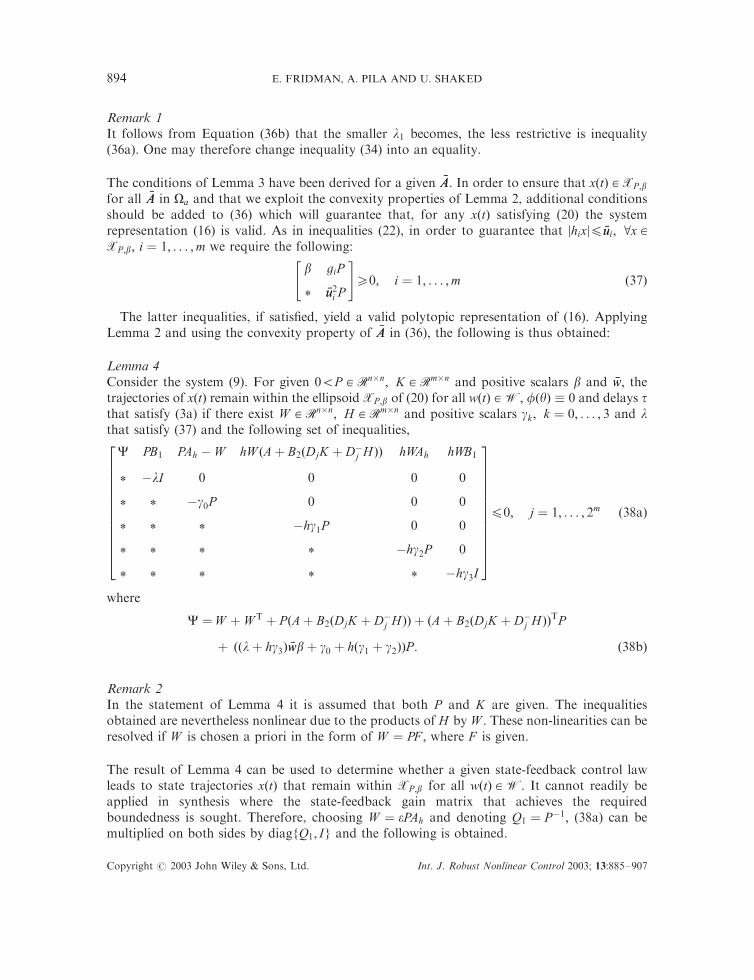
Remark 1It follows from Equation (36b) that the smaller l1 becomes, the less restrictive is inequality(36a). One may therefore change inequality (34) into an equality.

The conditions of Lemma 3 have been derived for a given %AA: In order to ensure that xðtÞ 2 XP ;b

for all %AA in Oa and that we exploit the convexity properties of Lemma 2, additional conditionsshould be added to (36) which will guarantee that, for any xðtÞ satisfying (20) the systemrepresentation (16) is valid. As in inequalities (22), in order to guarantee that jhixj4 %uui; 8x 2XP ;b; i ¼ 1; . . . ;m we require the following:

b giP

* %uu2i P

" #50; i ¼ 1; . . . ;m ð37Þ

The latter inequalities, if satisfied, yield a valid polytopic representation of (16). ApplyingLemma 2 and using the convexity property of %AA in (36), the following is thus obtained:

Lemma 4Consider the system (9). For given 05P 2 Rn�n; K 2 Rm�n and positive scalars b and %ww; thetrajectories of xðtÞ remain within the ellipsoid XP ;b of (20) for all wðtÞ 2 W; fðyÞ � 0 and delays tthat satisfy (3a) if there exist W 2 Rn�n; H 2 Rm�n and positive scalars gk ; k ¼ 0; . . . ; 3 and lthat satisfy (37) and the following set of inequalities,

C PB1 PAh � W hW ðAþ B2ðDjK þ D�j H ÞÞ hWAh hWB1

* �lI 0 0 0 0

* * �g0P 0 0 0

* * * �hg1P 0 0

* * * * �hg2P 0

* * * * * �hg3I

2666666666664

377777777777540; j ¼ 1; . . . ; 2m ð38aÞ

where

C ¼W þ W T þ P ðAþ B2ðDjK þ D�j H ÞÞ þ ðAþ B2ðDjK þ D�

j H ÞÞTP

þ ððlþ hg3Þ %wwbþ g0 þ hðg1 þ g2ÞÞP : ð38bÞ

Remark 2In the statement of Lemma 4 it is assumed that both P and K are given. The inequalitiesobtained are nevertheless nonlinear due to the products of H by W : These non-linearities can beresolved if W is chosen a priori in the form of W ¼ PF ; where F is given.

The result of Lemma 4 can be used to determine whether a given state-feedback control lawleads to state trajectories xðtÞ that remain within XP ;b for all wðtÞ 2 W: It cannot readily beapplied in synthesis where the state-feedback gain matrix that achieves the requiredboundedness is sought. Therefore, choosing W ¼ ePAh and denoting Q1 ¼ P�1; (38a) can bemultiplied on both sides by diagfQ1; Ig and the following is obtained.



Lemma 5Consider the system (9) with the feedback control law (6). Given positive scalars b and %ww; thetrajectories of xðtÞ remain within the ellipsoid XP ;b of (20), for some 05P 2 Rn�n and for allwðtÞ 2 W; fðyÞ � 0 and delays t that satisfy (3a) if there exist 05Q1 2 Rn�n; Y and G 2 Rm�n

and positive scalars gk ; k ¼ 0; . . . ; 3 and l that satisfy (22) and the following set of inequalities:

C1j B1 ð1� eÞAh ehðAQ1 þ B2ðDjY þ D�j GÞÞ ehAhQ1 ehB1

* �lI 0 0 0 0

* * �g0Q1 0 0 0

* * * �hg1Q1 0 0

* * * * �hg2Q1 0

* * * * * �hg3I

2666666666664

3777777777775

40; j ¼ 1; . . . ; 2m ð39aÞ

where

C1j ¼ ðAþ eAhÞQ1 þ Q1ðAT þ eATh Þ þ B2ðDjY þ D�

j GÞ þ ðY TDj þ GTD�j ÞB

T2

þ ððlþ hg3Þ %wwbþ g0 þ hðg1 þ g2ÞÞQ1 ð39bÞ

The matrix P is then given by P ¼ Q�11 and the feedback gain matrix which leads to xðtÞ 2 XP ;b is

given by K ¼ YQ�11 :

3.5. H1 control

The H1 performance is achieved if

d

dtV þ zTðtÞzðtÞ � g2wTðtÞwðtÞ50

where V is given by (18). Similarly to Theorem 1, we obtain the following.

Lemma 6The inequality (8) holds for a given K 2 Rm�n if the conditions of Lemma 5 are satisfied andthere exist *PP; of the form of (19), and *ZZ 2 R2n�2n; S; R 2 Rn�n; %WW 2 Rn�2n and H 2 Rm�n thatsatisfy the following.

%CCj *PPT0

B1

" #*PPT

0

Ah

" #� %WWT

CTj

0

" #

* �g2I 0 0

* * �ð1� dÞS�1 0

* * * �1

2666666664

377777777550; j ¼ 1; . . . ; 2m ð40aÞ

R�1 %WW

**ZZ

" #50 ð40bÞ



where

%CCj ¼ *PPT0 I

Aj þ B2ðDjK þ D�j H Þ �I

" #þ

0 ATj þ ðKTDj þ HTD�

j ÞBT2

I �I

" #*PP

þS�1 0

0 hR�1

" #þ ½ %WWT 0 � þ

%WW

0

" #

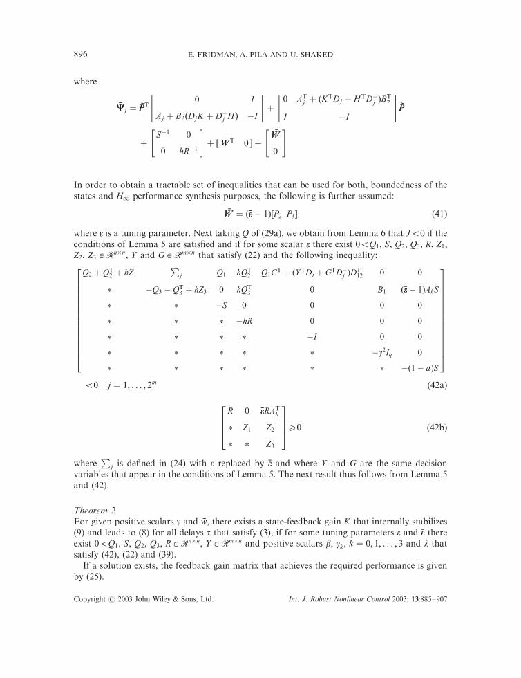
In order to obtain a tractable set of inequalities that can be used for both, boundedness of thestates and H1 performance synthesis purposes, the following is further assumed:

%WW ¼ ð%ee� 1Þ½P2 P3� ð41Þ

where %ee is a tuning parameter. Next taking Q of (29a), we obtain from Lemma 6 that J50 if theconditions of Lemma 5 are satisfied and if for some scalar %ee there exist 05Q1; S; Q2; Q3; R; Z1;Z2; Z3 2 Rn�n; Y and G 2 Rm�n that satisfy (22) and the following inequality:

Q2 þ QT2 þ hZ1

Pj Q1 hQT

2 Q1CT þ ðY TDj þ GTD�j ÞD

T12 0 0

* �Q3 � QT3 þ hZ3 0 hQT

3 0 B1 ð%ee� 1ÞAhS

* * �S 0 0 0 0

* * * �hR 0 0 0

* * * * �I 0 0

* * * * * �g2Iq 0

* * * * * * �ð1� dÞS

2666666666666664

3777777777777775

50 j ¼ 1; . . . ; 2m ð42aÞ

R 0 %eeRATh

* Z1 Z2

* * Z3

2664

377550 ð42bÞ

whereP

j is defined in (24) with e replaced by %ee and where Y and G are the same decisionvariables that appear in the conditions of Lemma 5. The next result thus follows from Lemma 5and (42).

Theorem 2For given positive scalars g and %ww; there exists a state-feedback gain K that internally stabilizes(9) and leads to (8) for all delays t that satisfy (3), if for some tuning parameters e and %ee thereexist 05Q1; S; Q2; Q3; R 2 Rn�n; Y 2 Rm�n and positive scalars b; gk ; k ¼ 0; 1; . . . ; 3 and l thatsatisfy (42), (22) and (39).

If a solution exists, the feedback gain matrix that achieves the required performance is givenby (25).



The conditions of Theorem 2 depend on the upper-bound of the delay length h: Correspondingdelay-independent conditions that provide a result that is valid for all 05h and ’tt4d are readilyobtained from Theorem 2 by letting e ¼ %ee ¼ 0; R ¼ r�1In; Z ¼ 0 and r; g1; g2; g3 ! 0: Thefollowing result is obtained.

Corollary 1For given positive scalars g and %ww; there exists a state-feedback gain K which for zero initialconditions leads to (8) for all wðtÞ 2 W; independently of the delay length and for ’tt4d; if thereexist if for some scalar e there exist 05Q1; S; Q2; Q3; R 2 Rn�n; Y and G 2 Rm�n and positivescalars b; g0 and l that satisfy (22) and the following set of inequalities:

Q2 þ QT2

Pj 0 0 Q1 Q1CT þ ðY TDj þ GTD�

j ÞDT12

* �Q3 � QT3 B1 AhS 0 0

* * �g2Iq 0 0 0

* * * �ð1� dÞS 0 0

* * * * �S 0

* * * * * �I

2666666666664

377777777777550 ð43aÞ

and

AQ1 þ Q1AT þ B2ðDjY þ D�j GÞ þ ðY TDj þ GTD�

j ÞBT2 þ ðl %ooþ g0ÞQ1 B1 AhQ1

* �lI 0

* * �g0Q1

2664

3775

40; j ¼ 1; . . . ; 2m ð43bÞ

ðl %wwþ g0Þ40 ð43cÞ

whereP

j is defined in (24), with e replaced by zero.If a solution exists, the feedback gain matrix that achieves the required performance is given

by (25).

Remark 3The results of Theorem 2 assume that except for the time-delay, which satisfies (3), the matricesof the system model of (9) are all known. Treating the scalar parameters in the inequalities of thetheorem as tuning parameters, these inequalities become LMIs that are affine in the system’smatrices. These LMIs can thus be used to solve the H1 control problem in the case whenuncertainty is encountered in the matrices of the system. Assuming that this uncertainty is of thepolytopic type [16], a solution to the control problem is obtained by solving the inequalities ofTheorem 2 at each vertex of the uncertainly polytope.

3.6. Parameter varying solution

In (42a) the same Q1; Q2 and Q3 appear in all of the 2m inequalities. The solution to all of theinequalities in Theorem 2, if it exists, will lead to a local quadratic stability condition. The



requirement for quadratic stability imposes a serious constraint on the solution which will nowbe alleviated.

It is readily verified that (42a) is equivalent to

#QQT #AATj þ #AAj

#QQþ diagfhZ; 0g QTI 0

0 hI

" #0 0

B1 ð%ee� 1ÞAhS

" #

* �S 0

* hR

" #0

* * �g2Iq 0

* ð1� dÞS

" #

2666666666664

3777777777775

40; j ¼ 1; . . . ; 2m ð44aÞ

where

#QQ ¼ diagfQ; 12Ipg ð44bÞ

#AAj ¼ #AA0 þ

0

B2

D12

2664

3775ðDjK þ D�

j H Þ½In 0� ð44cÞ

#AA0 ¼

0 In 0

Aþ eAh �In 0

C 0 �Ip

2664

3775 ð44dÞ

Similarly, (39a) is equivalent to

##AA#AAj*QQþ *QQ ##AA#AAT

j

In

0

" #B1 ð1� eÞAh ehAhQ1 ehB1

� �

* �diagflIq; g0Q1; hg2Q1; g3Iqg

2664

377540; j ¼ 1; . . . ; 2m ð45aÞ

where

*QQ ¼ diagfQ1;Q1g ð45bÞ

##AA#AAj ¼##AA#AA0 þ

I

0

" #B2ðDjK þ D�

j H Þ½In In� ð45cÞ

##AA#AA0 ¼Aþ eAh þ f1In ehA

0 �h2g1In

" #ð45dÞ

and

f1 ¼12ððlþ hg3Þ %wwbþ g0 þ hðg1 þ g2ÞÞ ð45eÞ

The following is applied to (44) and (45).



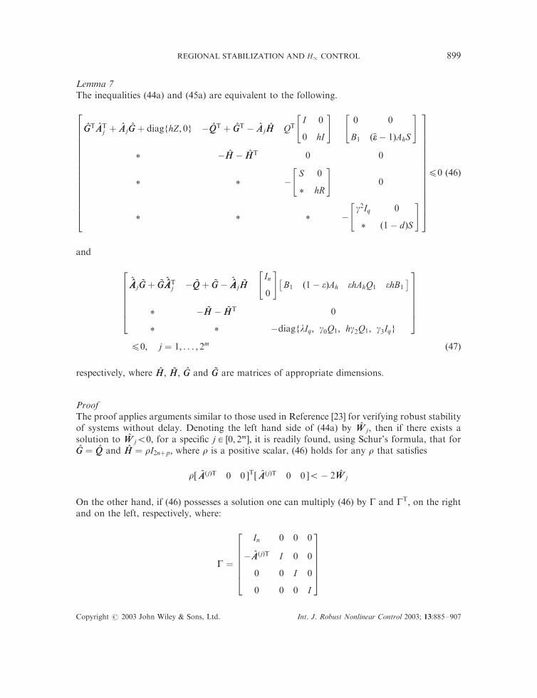
Lemma 7The inequalities (44a) and (45a) are equivalent to the following.

#GGT #AATj þ #AAj #GGþ diagfhZ; 0g � #QQT þ #GGT � #AAj #HH QT

I 0

0 hI

" #0 0

B1 ð%ee� 1ÞAhS

" #

* � #HH � #HHT 0 0

* * �S 0

* hR

" #0

* * * �g2Iq 0

* ð1� dÞS

" #

26666666666666664

37777777777777775

40 ð46Þ

and

##AA#AAj*GGþ *GG ##AA#AAT

j � *QQþ *GG� ##AA#AAj *HHIn

0

" #B1 ð1� eÞAh ehAhQ1 ehB1

� �

* � *HH � *HHT 0

* * �diagflIq; g0Q1; hg2Q1; g3Iqg

2666664

3777775

40; j ¼ 1; . . . ; 2m ð47Þ

respectively, where #HH; *HH; #GG and *GG are matrices of appropriate dimensions.

ProofThe proof applies arguments similar to those used in Reference [23] for verifying robust stabilityof systems without delay. Denoting the left hand side of (44a) by #WW j; then if there exists asolution to #WW j50; for a specific j 2 ½0; 2m�; it is readily found, using Schur’s formula, that for#GG ¼ #QQ and #HH ¼ rI2nþp; where r is a positive scalar, (46) holds for any r that satisfies

r½ #AAðjÞT 0 0 �T½ #AAðjÞT 0 0 �5� 2 #WW j

On the other hand, if (46) possesses a solution one can multiply (46) by G and GT; on the rightand on the left, respectively, where:

G ¼

In 0 0 0

� #AAðjÞT I 0 0

0 0 I 0

0 0 0 I

2666664

3777775



The resulting LMI is then

#WW j

� #QQþ #GGT þ #AAðjÞ #HHT

0

" #

* � #HH � #HHT

2664

377550 ð48Þ

and (44a) clearly follows. Similar arguments are applied to (47) and (45). &

The inequalities of Lemma 7 are now ready to be applied to the uncertain case. In the case wherethe matrices of the system are not exactly known, we assume that they belong toO 2 CofOj; j ¼ 1; . . . ; %NNg; where,

O ¼X%NN

j¼1

fj %OOj for some 04fj41;X%NN

j¼1

fj ¼ 1 ð49Þ

where the %NNð %NN > 2mÞ vertices of the polytope are described by

Oj ¼ ½AðjÞ AðjÞh BðjÞ

1 CðjÞ Dj �

It is assumed, for simplicity, that the matrices B2 and D12 in (9) and (10) are known.Defining the structures:

#GGj ¼G1 0

GðjÞ2 GðjÞ

3

" #ð50aÞ

#HHj ¼a1G1 0

H ðjÞ2 H ðjÞ

3

" #ð50bÞ

*GGj ¼a2G1 0

*GGðjÞ2

*GGðjÞ3

" #ð50cÞ

*HHj ¼a3G

ðjÞ1 0

*HHðjÞ2

*HHðjÞ3

24

35 ð50dÞ

Qj ¼QðjÞ

1 0

QðjÞ2 QðjÞ

3

24

35 ð50eÞ

for some positive scalars ai; i ¼ 1; 2; 3; we apply Lemma 7 to Theorem 2 and obtain thefollowing.

Theorem 3For given positive scalars g and %ww; there exists a state-feedback gain K that internally stabilizes(9), over the uncertainty polytope O and leads to (8) for all delays t that satisfy (3), if for somepositive tuning parameters e; %ee and ai; i ¼ 1; 2; 3 there exist Qj 2 R2n�2n of the structure (50e),with 05QðjÞ

1 ; #GGj; #HHj 2 Rð2nþpÞ�ð2nþpÞ of the structure (50a) and (50b), with 05G1; *GGj; *HHj 2R2n�2n of the structure (50c) and (50d), Zj 2 Rð2nþpÞ�ð2nþpÞ; 05Q1j; Rj 2 Rn�n; j ¼ 1; . . . ; %NN;



positive scalars l; %ll; b; gi; i ¼ 0; . . . ; 3; S 2 Rn�n and Y ; G 2 Rm�n that satisfy the following forj ¼ 1; . . . ; %NN:

PðjÞ1 � #QQT

j þ #GGTj � #AA

ðjÞ0

#HHj � a1

0

B2

D12

2664

3775ðDjY þ D�

j GÞ½In 0� QTj

I 0

0 hI

" #0 0

BðjÞ1 ð%ee� 1ÞAðjÞ

h S

" #

* � #HHj � #HHj 0 0

* * �S 0

* hRj

" #0

* * * �g2Iq 0

* ð1� dÞS

" #

26666666666666666664

37777777777777777775

40

ð51aÞ

PðjÞ1

¼ #GGTj#AAðjÞT0 þ #AA

ðjÞ0

#GGj þ

0

B2

D12

2664

3775ðDjY þ D�

j GÞ½In 0� þIn

0

" #ðY TDj þ GTD�

j Þ

0

B2

D12

2664

3775T

þ diagfhZj; 0g ð51bÞ

PðjÞ2 �diagfQ1j;Q1jg þ *GGj �

##AA#AAðjÞ0

*HHj � a2In

0

" #B2ðDjY þ D�

j GÞIn

In

" #TIn

0

" #BðjÞ1 ð1� eÞAh ehAhQ1j ehBðjÞ

1

h i

* � *HHj � *HHTj 0

* * �diagflIq; g0Q1j; hg2Q1j; g3Iqg

26666664

3777777540

ð52aÞ

PðjÞ2

¼ ##AA#AAðjÞ0

*GGj þ *GGj##AA#AAðjÞT0 þ

In

0

" #B2ðDjY þ D�

j GÞ½In In� þIn

In

" #ðY TDj þ GTD�

j ÞBT2 ½In 0� ð52bÞ

b gi

* ~uu2i QðjÞ1

" #50 ð53aÞ

and

QðjÞ1 I

*%llI

24

3550 ð53bÞ



where %ll is minimized and where

#AAðjÞ0 ¼

0 In 0

AðjÞ þ eAðjÞh �In 0

CðjÞ 0 �Ip

26664

37775 and ##AA#AA

ðjÞ0 ¼

AðjÞ þ eAðjÞh þ f1In ehAðjÞ

0 �h2g1In

" #

The feedback gain matrix which achieves the required performance is given by:

K ¼ Y ðG1Þ�1 ð54Þ

4. EXAMPLES

4.1. Stabilization

We consider the stabilization example of Reference [8]. The system of (9) was considered therewhere

A ¼0:5 �1

0:5 �0:5

" #; Ad ¼

0:6 0:4

0 �0:5

" #; B2 ¼

1

1

" #

and where %uu ¼ 5:In Reference [8] stabilization via state-feedback was obtained for delays that are less than or

equal to h ¼ 0:35: For t ¼ 0:35 the maximum radius of the stability ball achieved was 0.968.Applying the theory of Theorem 1 a stabilizing state-feedback controller has been obtained forall delays that are less than or equal to h ¼ 1:854: For the latter delay, with d ¼ 0; namelyconstant delay of t ¼ 1:854 the stabilizing gain was K ¼ �½25:8809 4:9315� with a stability ballradius of d1 ¼ d2 ¼ 0:091: This result was obtained for e ¼ 0:89 and b ¼ 1: The latter radiusincreases significantly when h decreases. For, say, h ¼ 0:35; 1; 1:8 the corresponding radii were(again d1 ¼ d2Þ 2:852; 1:7442; 0:8032; respectively. The stabilization theory of Theorem 1 resultsin state trajectories, for h ¼ 0:35; which begin on the periphery of the inner circle, never leave theouter ellipse and end up at the origin (see Figure 1).

4.2. H1 control

We consider the example that appeared in References [11] and [8]. The system (1) is describedby:

A ¼1 1:5

0:3 �2

" #; Ah ¼

0 �1

0 0

" #; B2 ¼

10

1

" #ð55Þ

We assume that h ¼ 1 s; d ¼ 0 and u0 ¼ 15: In Reference [11], quadratically local stabilizationwas achieved for all initial conditions in wd (and b ¼ 0 in their paper) with a dmax558:395:

Application of Theorem 1 (in the present paper), resulted in a value of d1 ¼ d2 ¼ dmax ¼79:43; which was obtained for e ¼ 1 and b ¼ 1: The corresponding state-feedback gain and Hwere:

K ¼ �7:913 0:7323� �

and H ¼ � 0:1534 0:0164� �



At this juncture we note the following points:

* The above value of H implies that the input to the actuators may exceed %uu during operation.* As should be expected, the result is insensitive to the value of b: The task of the latter

parameter is to scale the elements in P :* The result we obtained for dmax is better than the one obtained by Tarbouriech et al. [11] and

Cao et al. [8] for initial functions with small enough derivatives. Taking for example d2 ¼ 0; amaximum value of d1 ¼ 97:19 is achieved. The improvement in dmax is partially due to thedelay-dependent criterion used.

* The strength of the descriptor approach lies in its delay-dependent conditions. The theorydeveloped in Reference [11] is, however, delay-independent. Applying our delay-independentversion of Theorem 1 (letting e ¼ 0 in (21)), values of d1 ¼ d2 ¼ 63:79 were achieved alongwith a gain vector of

K ¼ �109½5:223 2:596�

-6 -4 -2 0 2 4 6

-5

-4

-3

-2

-1

0

1

2

3

4

5

x1

x2

Figure 1. Stabilization result: delay ¼ 0:35 s; inner circle radius ¼ d1 ¼ d2 ¼ 2:852;outer ellipse xTP1x4b�1 ¼ 1:



Even this delay-independent result compares favourably to the one which appeared inReference [11].

* The above numerical results were obtained for d ¼ 0; namely for the situation where thedelay t can reside anywhere in ½0 h� but is time invariant. The fact that our solution wasobtained for e ¼ 1 implies, however, that it holds true for any time varying delay whichsatisfies (3a) [21].

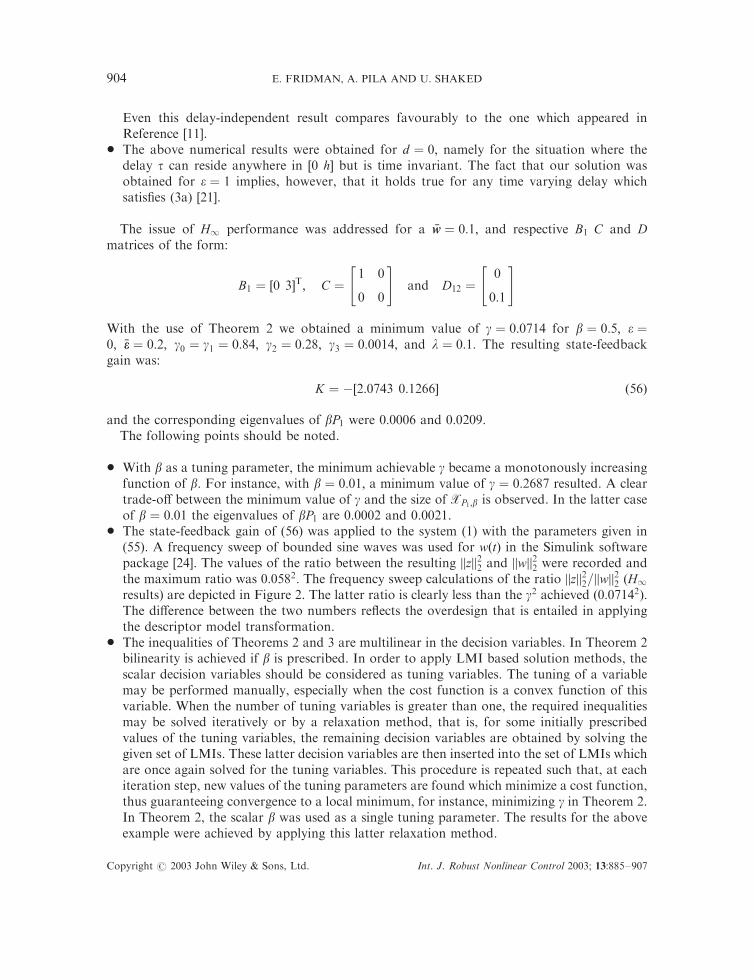
The issue of H1 performance was addressed for a %ww ¼ 0:1; and respective B1 C and Dmatrices of the form:

B1 ¼ ½0 3�T; C ¼1 0

0 0

" #and D12 ¼

0

0:1

" #

With the use of Theorem 2 we obtained a minimum value of g ¼ 0:0714 for b ¼ 0:5; e ¼0; %ee ¼ 0:2; g0 ¼ g1 ¼ 0:84; g2 ¼ 0:28; g3 ¼ 0:0014; and l ¼ 0:1: The resulting state-feedbackgain was:

K ¼ �½2:0743 0:1266� ð56Þ

and the corresponding eigenvalues of bP1 were 0:0006 and 0:0209:The following points should be noted.

* With b as a tuning parameter, the minimum achievable g became a monotonously increasingfunction of b: For instance, with b ¼ 0:01; a minimum value of g ¼ 0:2687 resulted. A cleartrade-off between the minimum value of g and the size of XP1;b is observed. In the latter caseof b ¼ 0:01 the eigenvalues of bP1 are 0.0002 and 0.0021.

* The state-feedback gain of (56) was applied to the system (1) with the parameters given in(55). A frequency sweep of bounded sine waves was used for wðtÞ in the Simulink softwarepackage [24]. The values of the ratio between the resulting jjzjj22 and jjwjj22 were recorded andthe maximum ratio was 0:0582: The frequency sweep calculations of the ratio jjzjj22=jjwjj

22 (H1

results) are depicted in Figure 2. The latter ratio is clearly less than the g2 achieved ð0:07142Þ:The difference between the two numbers reflects the overdesign that is entailed in applyingthe descriptor model transformation.

* The inequalities of Theorems 2 and 3 are multilinear in the decision variables. In Theorem 2bilinearity is achieved if b is prescribed. In order to apply LMI based solution methods, thescalar decision variables should be considered as tuning variables. The tuning of a variablemay be performed manually, especially when the cost function is a convex function of thisvariable. When the number of tuning variables is greater than one, the required inequalitiesmay be solved iteratively or by a relaxation method, that is, for some initially prescribedvalues of the tuning variables, the remaining decision variables are obtained by solving thegiven set of LMIs. These latter decision variables are then inserted into the set of LMIs whichare once again solved for the tuning variables. This procedure is repeated such that, at eachiteration step, new values of the tuning parameters are found which minimize a cost function,thus guaranteeing convergence to a local minimum, for instance, minimizing g in Theorem 2.In Theorem 2, the scalar b was used as a single tuning parameter. The results for the aboveexample were achieved by applying this latter relaxation method.



5. CONCLUSIONS

In the present paper, a delay-dependent LMI based sufficient condition has been proposed forstabilization and H1 control of linear systems with time varying delay. This feat wasaccomplished by combining the transformation of a single linear system with m possiblysaturated actuator channels into a set of 2m linear systems embedded within a convex polytopewith the Lyapunov-Krasovskii technique via descriptor model transformation. The merits of thedescriptor model approach lie in the fact that a smaller number of cross terms require bounding,thus resulting in a reduction of the over-design. The boundedness of the trajectories for systemswith bounded peak inputs has been treated by Razumikhin approach via first order modeltransformation.

In both the designs for stabilization and performance satisfaction, a serious source ofover-design arises from the quadratic stabilizability inherent in the design procedurefor polytopic systems. In order to alleviate this problem, a method wherein a differentLyapunov candidate function is assigned to each vertex of the polytope, was used, thus resultingin a further reduction of the conservativeness of the design. For the express purpose ofcomparing delay-dependent and delay-independent designs, a tuning parameter e was

0 0.5 1 1.5 2 2.5 3 3.5 4 4.5 50.025

0.03

0.035

0.04

0.045

0.05

0.055

0.06

freq [rad/sec]

max

z /

max

w

Figure 2. Deterministic frequency sweep from 0 to 5 rad=s with 20 random phase values at each frequency.



introduced which facilitates the switch between delay-dependent ðe=0Þ and delay-independentdesigns ðe ¼ 0Þ:

One of the drawbacks of the proposed method is that the domain of attraction depends on thederivative of the initial function. The proposed method for regional stabilization may thus beuseful in the case of neutral type systems where it is natural to consider initial functions from thespace C1:

ACKNOWLEDGEMENTS

This work was supported by the C&M Maus Chair at Tel Aviv University.

REFERENCES

1. Bernstein DS, Michel AN (eds). Special issue on saturating actuators. International Journal of Robust and NonlinearControl 1995; 5:375–540.

2. Saberi A, Stoorvogel AA (eds). Special issue on control problems with constraints. International Journal of Robustand Nonlinear Control 1999; 9:583–734.

3. Saberi A, Lin Z, Teel AR. Control of linear systems with saturating actuators. IEEE Transactions on AutomaticControl 1996; 41:368–378.

4. Lin Z. H1-Almost disturbance decoupling with internal stability for linear systems subject to input saturation. IEEETransactions on Automatic Control 1997; 42:992–995.

5. Gomes da Silva J, Fischman A, Tarbouriech S, Dion J, Dugard L. Synthesis of state feedback for linear systemssubject to control saturation by an LMI-based approach. Proceedings of ROCOND, Budapest, Hungary, June1997:219–234.

6. Hu T, Lin Z, Chen B. An analysis and design method for linear systems subject to actuator saturation anddisturbance. Automatica 2002; 38:351–359.

7. Chen BS, Wang SS, Lu HC. Stabilization of time-delay systems containing saturating actuators. InternationalJournal of Control 1988; 47:867–881.

8. Cao Y, Lin Z, Hu T. Stability analysis of linear time-delay systems subject to input saturation. IEEE Transactions onCircuits and Systems-I 2002; 49:233–240.

9. Hindi H, Boyd S. Analysis of linear systems with saturating using convex optimization. Proceedings of the 37thCDC, Florida, USA, December 1998:903–908.

10. Niculescu SI, Dion JM, Dugard L. Robust stabilization for uncertain time-delay systems containing saturatingactuators. IEEE Transactions on Automatic Control 1996:41:742–747.

11. Tarbouriech S, Gomes da Silva J. Synthesis of controllers for continuous-time delay systems with saturating controlsvia LMI’s. IEEE Transactions on Automatic Control 2000; 45:105–111.

12. Tarbouriech S, Peres PLD, Garcia G, Queinnic I. Delay-dependent stabilization of time-delay systems withsaturating actuators. 39th IEEE Conference on Decision and Control, Sidney, Australia, December 2000:3248–3254.

13. Cao Y, Lin Z, Hu T. Stability analysis of linear time-delay systems subject to input saturation. IEEE Transactions onCircuits and Systems 2002; 49:233–240.

14. Molchanov A, Pyatnitskii E. Criteria of asymptotic stability of differential and difference inclusions encountered incontrol theory. Systems & Control Letters 1989; 13:59–64.

15. Fridman E, Shaked U. On reachable sets for linear systems with delay and bounded peak inputs. Automatica, toappear.

16. Boyd S, El Ghaoui L, Feron E, Balakrishnan V. Linear Matrix Inequality in Systems and Control Theory. SIAMFrontier Series: Philadelphia, April 1994.

17. Fridman E. New Lyapunov-Krasovskii functionals for stability of linear retarded and neutral type systems. Systems& Control Letters 2001; 43:309–319.

18. Fridman E, Shaked U. A descriptor system approach to H1 control of linear time-delay systems. IEEE Transactionson Automatic Control 2002; 47:253–270.

19. Moon YS, Park P, Kwon WH, Lee YS. Delay-dependent robust stabilization of uncertain state-delayed systems.International Journal of Control 2001; 74:1447–1455.

20. Niculescu SI. Delay Effects on Stability: A Robust Control Approach. Lecture Notes in Control and InformationSciences. Vol. 269, Springer, London: 2001.



21. Fridman E, Shaked U. An improved stabilization method for linear time-delay systems. IEEE Transactions onAutomatic Control 2002; 47:1931–1937.

22. Hale J, Lunel S. Introduction to Functional Differential Equations. Springer: New York, 1993.23. Peaucelle D, Arzelier D, Bachelier O, Bernussou J. A new robust D-stability condition for real convex polytopic

uncertainty. Systems & Control Letters 2000; 40:21–30.24. Simulink. Dynamic System Simulation for Matlab. The Math Works, Inc. 1999.



Regional stabilization and H control of time-delay systems ...emilia/papers/spec.pdf ·...

Documents

Transcript of Regional stabilization and H control of time-delay systems ...emilia/papers/spec.pdf ·...