ORI GIN AL PA PER

Regional landslide susceptibility: spatiotemporalvariations under dynamic soil moisture conditions

Ram L. Ray • Jennifer M. Jacobs • Thomas P. Ballestero

Received: 15 February 2011 / Accepted: 25 April 2011� Springer Science+Business Media B.V. 2011

Abstract Quantification of landslide susceptibility variability in space and time in

response to static and dynamic conditions is a fundamental research challenge. Here, we

identify and apply new modeling and remote sensing observation techniques to statistically

characterize susceptibility distributions under dynamic moisture conditions. The methods

are applied at two study regions: Cleveland Corral, California, US and Dhading, Nepal.

The results show that the temporal variability of safety factors is lower during the wet

season than the dry season, but this variability, when scaled by mean seasonal stability, is

constant annually. Relative variability differs by region with lower variability in Nepal, the

highly susceptible region. L-Moment evaluations indicate that Nepal has a consistent,

regional probability distribution, but that California has two distinct distributions. The

variability in time is not normally distributed for either region. For both regions, transi-

tional characteristic of safety factors show a strong power law relationship between the

average duration and number of periods during which sites are highly susceptible. Because

the mapped landslide locations typically had frequent crossings with brief unstable con-

ditions, a consistent physical mechanism is pointed to as a possible cause of slope failure.

Keywords Landslide � Transitional � Safety factor � Variability � Spatiotemporal

1 Introduction

Shallow slope failures are common throughout the world in mountainous regions (Borga

et al. 1998; Gulla et al. 2008). Landslides, whether they are large or small in size, occur

every year in mountainous regions of the world (Li et al. 2010). Intrinsic variables

R. L. Ray (&)Department of Civil, Construction and Environmental Engineering, San Diego State University,5500 Campanile Dr., San Diego, CA 92182, USAe-mail: ramlakhan37@gmail.com

J. M. Jacobs � T. P. BallesteroEnvironmental Research Group, Department of Civil Engineering,University of New Hampshire, 35 Colovos Rd., Durham, NH 03824, USA

123

Nat HazardsDOI 10.1007/s11069-011-9834-4

(topography, geology, soil regolith and engineering properties) and extrinsic variables

(rainfall, fire, glacier outbursts, earthquakes and volcanoes) play critical roles in slope

stability (Dai and Lee 2002; Dahal et al. 2008; Cepeda et al. 2010).

To understand the physical and dynamic processes of instability, it is necessary to

quantify a region’s landslide susceptibility both in time and in space (Wu and Sidle 1995;

Glade 1998; Guzzetti et al. 1999; Stefanini 2004). Extrinsic variable changes can cause a

stable slope to become unstable. Of the extrinsic variables, rainfall is of interest because it

evolves as a transitional process that is highly variable at multiple scales in space and time

and has a strong interaction with the near surface. Rainfall-induced landslides are triggered

by wetting soils which effect a slope’s shear strength and the shear stress (Caine 1980;

Iverson and Major 1987; Rahardjo 2000; Lee 2005; Adler et al. 2006; Meisina and

Scarabelli 2007; Cepeda et al. 2010; Ray et al. 2010a).

Most studies only provide a static representation of landslide susceptibility (Li et al.

2010) or use rainfall characteristics that are indicative of soil wetting dynamics (e.g. spatial

distribution, duration and intensity) to predict landslide initiation (Iverson 2000; Lan et al.

2005; Dahal et al. 2008; Lee et al. 2008; Jaiswal and van Westen 2009; Turner et al. 2010;

Xu and Zhang 2010). However, rainfall alone is not adequate to identify slope instability.

For example, in order for Zezere et al. (2005) to identify the appropriate number of days

used to determine antecedent precipitation, they explicitly differentiated their method

based on landslide type and geo-environmental characteristics. Even for the shallow debris

slide investigated by Jaiswal and van Westen (2009), their envelope curves show con-

siderable variability across a modest-sized region. While these methods have advanced

considerably in regions that have a complete historical database on landslides and rainfall,

it remains a challenge to directly transfer site-specific methods using precipitation data to

other locations.

As a first-order process, slopes can become unstable when intense rainfall rapidly

increases soil water storage (Pelletier et al. 1997). Currently, the characteristics of land-

slide-prone regions’ soil moisture, the resulting evolution of slope instability in time and

the relative value of additional complexity are areas of active research for hill slope studies

(Jaiswal and van Westen 2009). For example, Talebi et al. (2008) used a hill slope model to

demonstrate that profile curvature effects slope stability magnitude and rates of change

during rain events.

Over longer periods and larger scales, soil moisture dynamics are linked to local veg-

etation and soil states that may be important to slope stability. While limited data exist for

steep terrain, a few studies have shown that vegetation type and rooting zone depths are

controlled by the evolution of soil moisture (Schwarz et al. 2010; Bathurst et al. 2010) and

the frequency of droughts (Oberhuber et al. 2001; Tosattig 2006). Soil wetting and drying

may also modify soil properties (Pires et al. 2008; Dorner et al. 2009) including cohesion

and porosity (Seguel and Horn 2006; Zemenu et al. 2009). Some of these effects have been

used in dynamic, distributed, physically based models to characterize the evolution of

quasi-static variables, vegetation strength and surcharge and their effects on landslide

susceptibility variability at monthly and annual time scales (Wu and Sidle 1995; Gorsevski

et al. 2006). While challenges remain in the prediction of susceptibility in space and time

because of soil and land cover heterogeneity as well as soil moisture variability (Saha et al.

2005), modelling and observational advancements are progressively reducing that uncer-

tainty (Davis and Keller 1997; Gorsevski et al. 2006).

This study seeks to use a dynamic, distributed, physically based model to capture the

large-scale, temporal evolution of safety factors for hazard-prone regions due to soil water

dynamics. Here, we propose that the characterization of daily soil water and attendant

Nat Hazards

123

safety factor variations over a multi-year period will show distinct slope stability spatio-

temporal patterns reflecting regional geo-environmental as well as climatic variables. This

characterization of landslide-prone slopes includes standard statistical moments,

L-moment methods and transition properties of threshold values. Two landslide-prone

regions, Cleveland Corral, California, US and Dhading, Nepal, are used to demonstrate and

contrast these metrics (Fig. 1a, b). Both sites include stable and unstable regions, but differ

by location, terrain, soils and climate.

2 Theory

This paper uses the modified infinite slope stability model to develop landslide suscepti-

bility that directly links vadose zone soil moisture and groundwater (Ray et al. 2010a). The

infinite slope method (Skempton and DeLory 1957) calculates safety factors as the ratio of

resisting forces to driving forces. The infinite slope stability model as adapted by the

several researchers (e.g. Montgomery and Dietrich 1994; van Westen and Terlien 1996;

Acharya et al. 2006; Ray and De Smedt 2009) is

FS ¼ Cs þ Cr

ceH sin hþ 1� m

cw

ce

� �tan utan h

ð1Þ

where Cs and Cr are the effective soil and root cohesion [kN/m2], ce is the effective unit

soil weight [kN/m3], H is the total depth of the soil above the failure plane [m], h is the

slope angle [�], m is the wetness index [dimensionless], / is the angle of internal friction of

the soil [�], and cw is the unit weight of water [kN/m3]. The effective unit weight is

estimated as

Fig. 1 a Mapped landslide (top) and slope movement (bottom) locations at Cleveland Corral, California in2006 and b a major catastrophic landslide along Prithvi Highway, Nepal (picture was taken in August, 2003)

Nat Hazards

123

ce ¼q cos h

Hþ ð1� mÞcd þ mcs ð2Þ

where q is any additional load on the soil surface [kN/m2] and cd is dry unit soil weight

[kN/m3] for the unsaturated soil layer.

Here, the wetness index follows Ray et al. (2010a) where

m ¼ hþ ðH � hÞ � Sw

Hð3Þ

where h is the saturated thickness of the soil [m] above the failure plane and Sw is the

degree of soil saturation [cm3/cm3] or vadose zone soil moisture.

The estimated safety factor (FS) values are categorized into stability classes using Pack

et al.’s (1998) and Acharya et al.’s (2006) stability classification system where the four

susceptibility classes are highly susceptible (FS B 1), moderately susceptible

(1 \ FS \ 1.25), slightly susceptible (1.25 \ FS \ 1.5) and not susceptible (stable)

(FS C 1.5). The critical threshold for slope failure occurs when the resisting force equals

the sliding force and the FS = 1 (Skempton and DeLory 1957; van Westen and Terlien

1996; Burton and Bathurst 1998; Acharya et al. 2006; Ray and De Smedt 2009).

Depending on the soil, vegetation and climatic characteristics of the region, a slope may or

may not fail at this critical safety factor value.

Application of the modified infinite slope stability model to time series analyses requires

a dynamic, distributed, physically based model. For this study, we use the VIC-3L model

(Liang et al. 1994) to estimate soil moisture in the unsaturated zone. VIC-3L is a mac-

roscale land surface model that was used to simulate the water budget based on the

climatic, soil and vegetation characteristics. Model details, application and validation are

provided in Ray et al. (2010b). The primary model output are daily, spatially distributed

predictions of saturated zone and vadose zone soil moisture that can be directly used to

determine the wetness index in Eq. 3 (Ray et al. 2010a).

3 Application

3.1 California, United States

The Cleveland Corral study region in the Highway 50 corridor is located in the Sierra

Nevada Mountains, California, USA (Reid et al. 2003). The study area is about 22 by

28 km or 616 km2. Highway 50 is a major road located between Sacramento and South

Lake Tahoe in California (Spittler and Wagner 1998). About 600 landslides were cat-

alogued along the 24-km-long corridor (Spittler and Wagner 1998; Reid et al. 2003). One

major catastrophic landslide occurred in 1983 (Spittler and Wagner 1998). Since 1996,

slope movement and landslides occur infrequently during the winter months. Slope

movement is defined as the transitional slow movement of slope without any slope

failures or landslides. Figure 1a shows one Cleveland Corral hill slope having mapped

landslide and slope movement. Since 1997, the United State Geological Survey (USGS)

has monitored this region using real-time data acquisition systems. The USGS obser-

vations found that elevated pore-water pressures and wet soils were coincident with

enhanced slope movement and landslides during the winter (rainy) season (Reid et al.

2003).

Nat Hazards

123

Elevations in this study area range from about 902–2,379 m. Based on the 90-m SRTM

digital elevation model (DEM), slopes in this region range from 0 to 48� with 1.27% of the

area possessing slopes greater than 30�. This study region has considerable variability in

soil texture ranging from clay loam to sandy loam (Table 1). The soil is predominantly

sandy loam (72%). The total soil depth ranges from 0.6 to 1.4 m. The assumed potential

failure plane underneath the soil layer is bedrock. Conifer and wooded grassland are the

dominant land covers: 80 and 14% of the study region, respectively. Some rock outcrops

were also observed along the Highway 50 corridor during the field observation.

The climatic data were obtained from the National Climatic Data Centre (NCDC) from

2003 to 2006 (Table 1). This region has average annual rainfall of 1,101 mm and maxi-

mum and minimum temperatures of 19.6 and 5.5�C, respectively. The majority of rainfall

occurs during the winter (725 mm) in this region. This region’s wet season is defined as

January to May.

Table 1 Soil, vegetation, slopeand climatic characteristics of theCalifornia and Nepal studyregions

Area (%)

California Nepal

Land cover

Evergreen forest 3.3 1.0

Conifer 79.9 –

Deciduous forest 2.7 –

Woodland – 50.3

Wooded grassland 14.1 18.2

Grassland – 1.7

Cropland – 28.8

Soil texture

Loamy sand – 16.2

Sandy loam 72.0 22.5

Loam 16.0 9.8

Sandy clay 3.0 15.0

Sandy clay loam – 36.5

Clay loam 9.0 –

Slope (�)

0–15 71.2 19.0

15–30 27.5 53.2

30–45 1.2 27.0

45–60 0.0 0.8

Climate

Average annual rainfall (mm) 1,101 1,624

Average rainfall wet season (mm)

(Jan–May, CA and Jun–Sep, Nepal) 725 1,287

Average daily max. temperature (�C) 19.6 27.0

Average daily min. temperature (�C) 5.5 16.6

Nat Hazards

123

3.2 Dhading, Nepal

The Nepal study area in the Dhading region is one of the seventy-five Nepalese districts.

The transnational Prithvi highway, connecting Kathmandu and Pokhara, runs through the

southern part of the district and parallels the Trishuli River. The study area is about 25 by

14 km or 350 km2. Landslides are frequent during the monsoon season (June to Sep-

tember). Numerous major landslides have occurred along the Prithvi highway over the past

decade (2000–2008) with a major catastrophic landslide at Krishna Bhir in August 2003

(Fig. 1b).

The Nepal study region has distinctly different topography, soil, vegetation and climatic

characteristics from the California region. The Nepal study region is 83% mountainous

terrain and 17% southern alluvial plains. Based on the SRTM DEM, elevations range from

256 to 1,918 m. Slopes in this region range from 0 to 57� with 27.8% of the study region’s

slopes exceeding 30�. The soils are predominantly sandy clay loam (36%) and sandy loam

(22%). Woodland and cropland are the dominant land covers: 50 and 29% of the study

region, respectively. The total soil depth ranges from 1.0 to 1.5 m. The assumed potential

failure plane underneath the soil layer is bedrock.

Rainfall, temperature and wind speed measurements were obtained from the Depart-

ment of Hydrology, Nepal (Table 1). This region is warmer and wetter than the California

study region. The monsoon season, June to September, averages 1,287 mm of the

1,624 mm average annual rainfall. Nepal’s wet season is defined as June to September.

3.3 Model data

For the California study region, the soil and vegetation data required for the three-layer

variable infiltration capacity (VIC-3L) hydrologic model and the slope stability model

were obtained from States Soil Geographic (STATSGO) database (Soil Survey Staff 2008),

Land Data Assimilation System (LDAS; Mitchell et al. 2004) and from the literature

(Table 2). The STATSGO soil data were obtained in vector format (polygon) and con-

verted into a 90-m raster (grid). For Nepal, soil depth and soil texture were assigned the

values from global and local databases as developed by Ray and De Smedt (2009). The

unit soil weight values (saturated and moist) were calculated from VIC-3L model soil

moisture estimates and literature values of soil porosity and specific gravity of the soils

(Table 2) using methods adapted by Ray et al. (2010a). For both regions, each land cover

class was assigned a root cohesion value adapted from Sidle and Ochiai (2006). Each soil

type was assigned soil cohesion and friction angle values from Deoja et al. (1991). The

slope of the retention curve is from Clapp and Hornberger (1978). Soil bulk density, field

capacity, wilting point and saturated hydraulic conductivity values are from Miller and

White (1998) and Dingman (2002). Slope angle was determined from a 90-m SRTM

digital elevation model (DEM). For both study regions, landslides locations were mapped

in the field using global positioning system (GPS). The field observations identified ten and

twelve landslides locations in California and Nepal, respectively.

4 Analysis methods

For these study regions, the VIC-3L model was applied at a daily time-step from October

2003 to September 2006 using a 0.0083� (*900-m) resolution. The Cleveland Corral,

California, US study region has 900 pixels sized at 0.7 km2 and Dhading, Nepal has 450

Nat Hazards

123

pixels sized at 0.75 km2. The VIC-3L soil moisture values were assigned to the 90-m DEM

pixels using a nearest neighbour approach. This study used soil moisture values approxi-

mately at 900-m and all other model parameters at 90-m scales. Using the VIC modelled

soil moisture, groundwater and geotechnical parameters, daily safety factors were calcu-

lated for each 90-m DEM pixels using Eqs. 1–3. In total, daily safety factors were

determined for 75,988 pixels in California and 41,800 pixels in Nepal from 1 October 2003

to September 30, 2006. The maximum modelled wetness was determined at each 90-m

pixel and used to classify the pixel’s susceptibility classes as highly, moderately, slightly

susceptible or not susceptible (stable). For each region and susceptibility class, a daily

average susceptibility was calculated to present dynamic susceptibility during the study

period.

Safety factor variations were characterized using a suite of descriptive statistics,

probability distributions analyses and crossing properties for the critical slope failure

threshold. Descriptive statistics included mean, standard deviation (SD), coefficient of

variation (CV) and skewness. Statistics were calculated for the entire year as well as for the

wet season. Statistics were mapped to indentify spatial patterns.

Probability distributions were examined using histograms, and goodness of fit was

considered using L-moment diagrams (Hosking 1990). While the method of moment

method is the traditional approach to fitting distributions, L-moment diagrams are often an

improvement because they are approximately unbiased and are particularly relevant when

samples are skewed (Vogel and Fennessey 1993). L-Moment diagrams, L-skewness (s3)

versus L-kurtosis (s4) and theoretical relationships for five probability distributions were

Table 2 List of model parameters and sources by model

Parameters Sources Model

Soil cohesion Deoja et al. (1991) Slope stability

Soil porosity Dingman (2002) Slope stability and VIC-3L

Soil texture STATSGO Slope stability and VIC-3L

Soil depth STATSGO Slope stability and VIC-3L

Hydraulic conductivity STATSGO VIC-3L

Soil bulk density Dingman (2002) Slope stability and VIC-3L

Angle of internal friction Deoja et al. (1991) Slope stability

Additional load (surcharge) Ray (2004) Slope stability

Land cover University of Maryland Slope stability and VIC-3L

Root cohesion Sidle and Ochiai (2006) Slope stability

Root depth LDAS VIC-3L

Root fraction LDAS VIC-3L

Vegetation roughness LDAS VIC-3L

Vegetation height LDAS VIC-3L

Leaf Area Index (LAI) LDAS VIC-3L

Rainfall NCDC, DOH-NP VIC-3L

Groundwater USGS Slope stability

Temperature NCDC, DOH-NP VIC-3L

Wind speed NCDC, DOH-NP VIC-3L

STATSGO States Soil Geographic, LDAS Land Data Assimilation System, USGS United States GeologicalSurvey, VIC-3L variable infiltration capacity-3 layers, NCDC National Climatic Data Center, DOH-NPDepartment of Hydrology, Nepal

Nat Hazards

123

constructed using the theory presented by Stedinger et al. (1993), Vogel and Wilson (1996)

and Hosking and Wallis (1997). L-Moment analysis is used to compare if the region has a

consistent probability distribution and, if so, which potential theoretical probability dis-

tribution best matches the observed probability distributions of the safety factors in highly

susceptible regions.

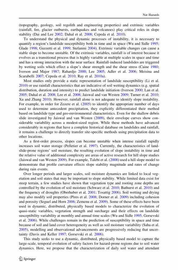
Crossing properties have been used extensively in soil moisture studies to identify

critical thresholds of plant water stress (e.g. Porporato et al. 2001). This concept is applied

to slope stability in order to present a statistical analysis of the duration and frequency of

instability. A crossing property analysis determines the number of crossings and the

average duration of all crossings. For this study, the critical crossing threshold is defined as

the transition from moderately susceptible to highly susceptible (Fig. 2). The crossing

duration corresponds to a single crossing and is the number of days that a pixel remains

classified as highly susceptible before returning to a moderately susceptible state. The

crossing properties are mapped and evaluated using observed landslide events.

5 Results and discussion

5.1 Dynamic landslide susceptibilities

Using the VIC modeled soil moisture, groundwater and geotechnical parameters, daily

safety factors were calculated for the study period (2003–2006) in the Nepal and California

study regions. The maximum modeled wetness was determined at each 90-m pixel and

used to classify the pixel’s susceptibility classes as highly, moderately, slightly susceptible

or not susceptible (stable). Regionally, Nepal has a much greater proportion of susceptible

area than California (Table 3).

For each region and susceptibility class, a daily average susceptibility was calculated as

the average safety factor value for all pixels in each study region and susceptibility class.

Figure 3 shows the time evolution of these average safety factors by region and class as

well as the threshold (FS = 1) indicating when a typical hazard-prone area becomes

Fig. 2 Demonstration of crossing and duration properties based on safety factor transitions from stable tounstable and return to stable

Nat Hazards

123

susceptible. The parallel time evolution across susceptibility classes is likely due to similar

climatic patterns for the regions. While hazardous seasons in California and Nepal differ,

the transition from dry (high FS) to wet conditions (low FS) occurs over a short period in

both regions. Intense rainfall, increasing vadose zone wetness and rising groundwater

levels, rapidly decrease safety factors. The regions’ safety factor variations during the wet

and dry seasons also differ. The California slopes have fairly large variations when they are

unstable, and, on average, a region is typically unstable for a short period of time. In Nepal,

once regions become unstable, they tend to stay unstable for the remainder of the monsoon

season with more limited variations. During stable periods, California’s slope stability is

fairly consistent due to relatively constant dry conditions. Nepal’s stable periods differ by

year. Some years have constant stability similar to California, while other years have

variations that are not markedly different than its unstable periods.

Descriptive statistics of the safety factors, mean, SD, CV and skewness, were calculated

for each pixel from the time series of daily safety factors at that pixel. The average and

standard deviation of these statistics are summarized by susceptibility category (Table 3).

On an annual basis, the average, SD and CV statistics are lower in Nepal than California.

Results show that these differences are not notable for the highly susceptible areas, but that

the range of conditions is much greater in California than Nepal. The SD typically

increases with decreasing susceptibility. The CV is nearly identical for all susceptible

classes. Statistics differ during the wet season as compared to the annual period. The

average, SD, and CV of the estimated safety factors are all lower during the wet season

than on an annual basis. The negative and positive skew during the annual period and wet

season, respectively, suggest that there are two distinct populations of safety factors

depending on the period of interest.

Table 3 Safety factor statistics for the 2003–2006 study period and wet season (Jan–May) for Californiaand (Jun–Sep) for Nepal

Statisticalparameter

California Nepal

Highlysusceptible

Moderatelysusceptible

Slightlysusceptible

Highlysusceptible

Moderatelysusceptible

Slightlysusceptible

Area (%) 0.49 1.69 2.89 11.59 23.30 21.12

Number of pixels 339 1,169 2,007 4,748 9,545 8,653

Annual

Average 1.09 (0.12) 1.44 1.75 1.02 (0.13) 1.30 1.57

SD 0.14 (0.03) 0.18 0.23 0.11 (0.03) 0.12 0.14

Skewness 0.03 (0.23) -0.05 -0.05 -0.09 (0.05) -0.09 -0.09

CV 0.13 (0.02) 0.12 0.13 0.10 (0.03) 0.09 0.08

Wet season

Average 0.98 (0.10) 1.29 1.56 0.92 (0.11) 1.19 1.43

SD 0.08 (0.02) 0.11 0.13 0.04 (0.01) 0.05 0.06

Skewness 1.10 (0.19) 1.10 1.12 1.37 (0.14) 1.39 1.39

CV 0.08 (0.02) 0.09 0.09 0.05 (0.01) 0.04 0.04

Parentheses indicate standard deviation. Classifications are based on maximum modeled susceptibility on8 May 2005 for California and 18 August 2004 for Nepal

CV coefficient of variance

Nat Hazards

123

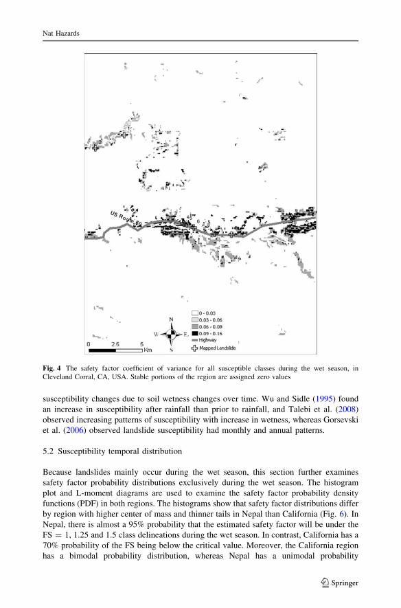
The spatial distribution of CV values for all susceptibility classes differs by location,

and there is some spatial coherence (Figs. 4, 5). The California study region has a higher

CV throughout the study area as compared to Nepal. This relative high variability may be

an indicator of regions with localized susceptible areas. Both study regions have a highway

and a river passing through the center of their study region. While the DEM scales make it

difficult to discern how the highway impacted regional susceptibility, the CVs along the

highway are very different between the two regions. In Nepal, a highway divides the steep

southern region from the modest slopes in the northern region which includes the river.

Very low CV values are found in the North along the river and highway with higher

variability along the steep southern terrain. In California, steep slopes border the highway,

and high CV values occur along the highway and stream. Thus, there is a strong geo-

morphic control that appears to be independent of the river or highway presence on

stability variations. The California study region also has lower CV values in the highly

susceptible class (Fig. 4) near to the natural water body (mapped landslide no. 1).

These landslide susceptibility variability results are comparable to the 3-day study by

Wu and Sidle (1995), the 20-day study by Talebi et al. (2008) and the 30-year temporal

susceptibility analysis by Gorsevski et al. (2006). These studies also identified landslide

0

50

100

150

2000.00

0.50

1.00

1.50

2.00

2.50

O-03 D-03 F-04 A-04 J-04 A-04 O-04 D-04 F-05 A-05 J-05 A-05 O-05 D-05 F-06 A-06 J-06 A-06

Rai

nfa

ll (m

m)

Saf

ety

Fact

or

RainfallHighly SusceptibleModerately SusceptibleSlightly Susceptible(b)

0

50

100

150

2000.00

0.50

1.00

1.50

2.00

2.50

O-03 D-03 F-04 A-04 J-04 A-04 O-04 D-04 F-05 A-05 J-05 A-05 O-05 D-05 F-06 A-06 J-06 A-06

Rai

nfa

ll (m

m)

Saf

ety

Fact

or

Rainfall

High Susceptible

Moderately Susceptible

Slightly Susceptible(a)

Fig. 3 a Average safety factors and rainfall distribution by susceptibility class at the Cleveland Corral, CA,USA study region; b average safety factors and rainfall distribution by susceptibility class at the Dhading,Nepal study region

Nat Hazards

123

susceptibility changes due to soil wetness changes over time. Wu and Sidle (1995) found

an increase in susceptibility after rainfall than prior to rainfall, and Talebi et al. (2008)

observed increasing patterns of susceptibility with increase in wetness, whereas Gorsevski

et al. (2006) observed landslide susceptibility had monthly and annual patterns.

5.2 Susceptibility temporal distribution

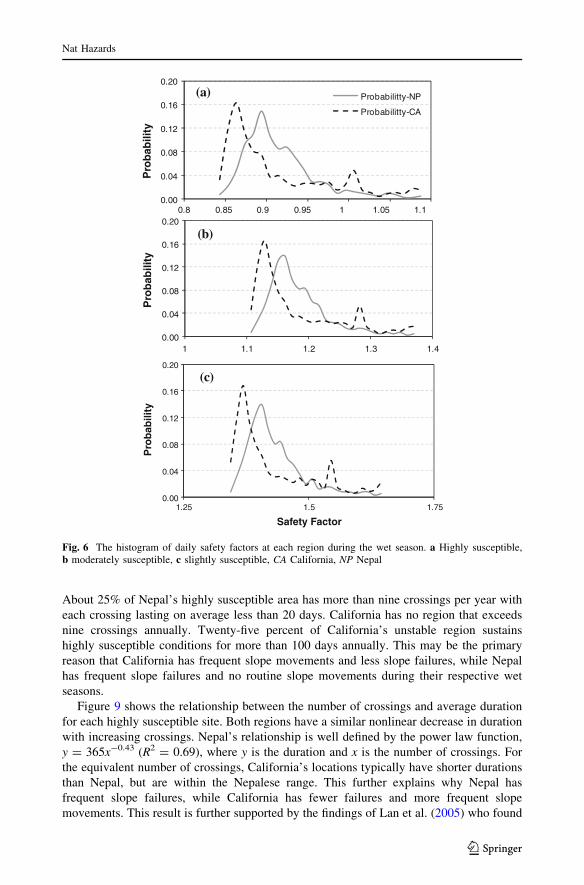
Because landslides mainly occur during the wet season, this section further examines

safety factor probability distributions exclusively during the wet season. The histogram

plot and L-moment diagrams are used to examine the safety factor probability density

functions (PDF) in both regions. The histograms show that safety factor distributions differ

by region with higher center of mass and thinner tails in Nepal than California (Fig. 6). In

Nepal, there is almost a 95% probability that the estimated safety factor will be under the

FS = 1, 1.25 and 1.5 class delineations during the wet season. In contrast, California has a

70% probability of the FS being below the critical value. Moreover, the California region

has a bimodal probability distribution, whereas Nepal has a unimodal probability

Fig. 4 The safety factor coefficient of variance for all susceptible classes during the wet season, inCleveland Corral, CA, USA. Stable portions of the region are assigned zero values

Nat Hazards

123

distribution. Results clearly show two populations of safety factors in California, and

therefore, this mode cannot be considered the best measure of central tendency as for

Nepal. Although both study regions have positively skewed safety factors, the California

region has less variability in susceptibility than Nepal.

For each highly susceptible site, the safety factors’ L-Skewness s3 and L-Kurtosis

s4 were computed and plotted for the wet season values. Figure 7 compares theoretical

probability distribution relationships to the individual L-moment values for each site as

well as the mean s3 and s4 values for each region. Nepal’s susceptible areas have a

consistent distribution that is distinctly different from the California region. For Nepal, the

clustering of sites indicates the region has a common probability distribution. The three-

parameter lognormal (LN3) distribution does a reasonable job of capturing the temporal

variability of safety factors for Nepal’s highly susceptible sites. The unstable areas in

California have one of three distinct populations. The two populations having a relatively

high kurtosis and following a generalized Pareto distribution are located near the natural

water body (mapped landslide no. 1). The region along the CA highway has a different,

distinct pattern with a much lower kurtosis. While the normal or gamma distributions are

frequently associated with hydrological processes, neither distribution fits the observed

variability for these landslide-prone regions. Thus, a single underlying distribution for

landslide susceptibility cannot be used for different locations.

5.3 Crossing properties of landslide safety factors

The crossing properties associated with the time evolution of stability were quantified for

each highly susceptible location (339 locations/pixels in California, 4,748 in Nepal).

Boxplots used to summarize these values show that California and Nepal have nearly equal

median crossing and duration values, but have different ranges (Fig. 8). The median

duration under the threshold is slightly shorter in California (18 days) than in Nepal

(26 days), whereas the median number of crossings is the same in Nepal and California.

Fig. 5 The safety factor coefficient of variance for all susceptible classes during the wet season in Dhading,Nepal. Stable portions of the region are assigned zero values

Nat Hazards

123

About 25% of Nepal’s highly susceptible area has more than nine crossings per year with

each crossing lasting on average less than 20 days. California has no region that exceeds

nine crossings annually. Twenty-five percent of California’s unstable region sustains

highly susceptible conditions for more than 100 days annually. This may be the primary

reason that California has frequent slope movements and less slope failures, while Nepal

has frequent slope failures and no routine slope movements during their respective wet

seasons.

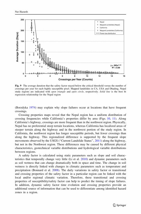
Figure 9 shows the relationship between the number of crossings and average duration

for each highly susceptible site. Both regions have a similar nonlinear decrease in duration

with increasing crossings. Nepal’s relationship is well defined by the power law function,

y = 365x-0.43 (R2 = 0.69), where y is the duration and x is the number of crossings. For

the equivalent number of crossings, California’s locations typically have shorter durations

than Nepal, but are within the Nepalese range. This further explains why Nepal has

frequent slope failures, while California has fewer failures and more frequent slope

movements. This result is further supported by the findings of Lan et al. (2005) who found

0.00

0.04

0.08

0.12

0.16

0.20

0.8 0.85 0.9 0.95 1 1.05 1.1

Pro

bab

ility

Probabilitty-NP

Probabilitty-CA

(a)

0.00

0.04

0.08

0.12

0.16

0.20

1 1.1 1.2 1.3 1.4

Pro

bab

ility

(b)

0.00

0.04

0.08

0.12

0.16

0.20

57.15.152.1

Pro

bab

ility

Safety Factor

(c)

Fig. 6 The histogram of daily safety factors at each region during the wet season. a Highly susceptible,b moderately susceptible, c slightly susceptible, CA California, NP Nepal

Nat Hazards

123

that while some slopes can fail rapidly, others can take a long time to fail under similar

saturation.

Landslide locations were mapped by each region (Figs. 4, 5), and their crossing

properties are indicated in Fig. 9. Interestingly, most of these highly susceptible regions

and mapped landslides have frequent crossings and briefly unstable conditions. Of the ten

mapped landslides in California, seven have short duration, unstable conditions and fre-

quent crossings. In Nepal, eleven out of the twelve slide locations have the same short

unstable conditions and frequent crossings. A gradual decrease or increase in stress over

time that causes cyclic stress relaxation associated with subsequent material failures

-0.20

0.00

0.20

0.40

0.00 0.10 0.20 0.30 0.40 0.50 0.60

L-K

urt

osi

s, τ

4

L-Skewness, τ3

Generalized Pareto (GPA)

Gamma (P3)

Lognormal (LN3)

Gumbel

Normal

California

Nepal

Mean SF-CA

Mean SF-NP

Fig. 7 L-Moment diagrams for each highly susceptible location by region and potential probabilitydistribution functions during the wet season for generalized Pareto (GPA), gamma (P3), normal, Gumbel andthree parameter lognormal (LN3) distributions

0

5

10

15

20

Nepal California

Nu

mb

er o

f cro

ssin

gs

0

50

100

150

200

250

Nepal California

Ave

rag

e d

ura

tion

(day

s)

(a) (b)

Fig. 8 The quantile box plots of a the number of transitions (crossings) below the safety factor thresholdvalue and b the average duration that the safety factor stayed below the threshold on an annual basis byregion (complete year)

Nat Hazards

123

(Borzdyka 1974) may explain why slope failures occur at locations that have frequent

crossings.

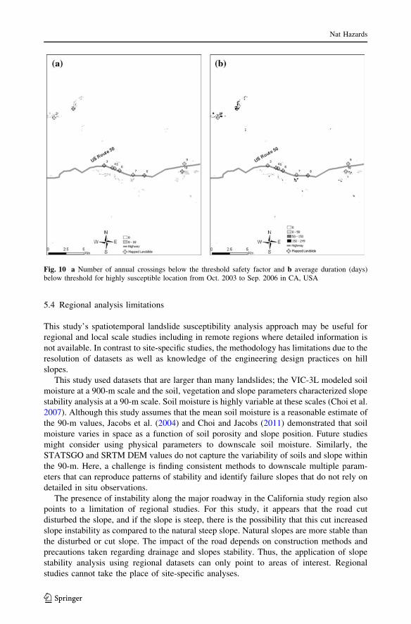
Crossing properties maps reveal that the Nepal region has a uniform distribution of

crossing frequencies while California’s properties differ by area (Figs. 10, 11). Along

California’s highway, crossings are more frequent than in the northwest region. Physically,

Nepal has no preferential steep terrain locations, whereas California has localized areas of

steeper terrain along the highway and in the northwest portion of the study region. In

California, the northwest region has longer susceptible periods, but fewer crossings than

along the highway. This regionalized difference is supported by the frequent slope

movements observed by the USGS (‘‘Current Landslide Status’’, 2011) along the highway,

but not in the Northwest region. These differences may be caused by different physical

characteristics, geotechnical variable distributions and hydrological variable distributions

between regions.

A safety factor is calculated using static parameters such as slope and soil charac-

teristics that temporally change very little (Li et al. 2010) and dynamic parameters such

as soil wetness that can change dramatically both in space and time. The change in soil

wetness is directly linked with changes in climatic parameters such as temperature and

precipitation (Bonnard et al. 2008). The daily variations in safety factor or transitional

and crossing properties of the safety factor in a particular region can be linked with the

local and/or regional climatic variation. Therefore, these transitional and crossing

properties of susceptibility/safety factor can help to predict the timing of slope failures.

In addition, dynamic safety factor time evolution and crossing properties provide an

additional source of information that can be used to differentiate among identified hazard

zones in a region.

y = 365x-0.43

R2 = 0.69

0

50

100

150

200

250

0 2 4 6 8 10 12 14 16

Ave

rag

e D

ura

tio

n (

Day

s)

Crossings per Year (Counts)

Nepal

Mapped Landslides (Nepal)

California

Mapped Landslides (California)

Power-law distribution

Fig. 9 The average duration that the safety factor stayed below the critical threshold versus the number ofcrossings per year for each highly susceptible pixel. Mapped landslides in CA, USA and Dhading, Nepalstudy regions are indicated with open triangle and open circle, respectively. Solid line is the best fitregression relationship for the Nepal region

Nat Hazards

123

5.4 Regional analysis limitations

This study’s spatiotemporal landslide susceptibility analysis approach may be useful for

regional and local scale studies including in remote regions where detailed information is

not available. In contrast to site-specific studies, the methodology has limitations due to the

resolution of datasets as well as knowledge of the engineering design practices on hill

slopes.

This study used datasets that are larger than many landslides; the VIC-3L modeled soil

moisture at a 900-m scale and the soil, vegetation and slope parameters characterized slope

stability analysis at a 90-m scale. Soil moisture is highly variable at these scales (Choi et al.

2007). Although this study assumes that the mean soil moisture is a reasonable estimate of

the 90-m values, Jacobs et al. (2004) and Choi and Jacobs (2011) demonstrated that soil

moisture varies in space as a function of soil porosity and slope position. Future studies

might consider using physical parameters to downscale soil moisture. Similarly, the

STATSGO and SRTM DEM values do not capture the variability of soils and slope within

the 90-m. Here, a challenge is finding consistent methods to downscale multiple param-

eters that can reproduce patterns of stability and identify failure slopes that do not rely on

detailed in situ observations.

The presence of instability along the major roadway in the California study region also

points to a limitation of regional studies. For this study, it appears that the road cut

disturbed the slope, and if the slope is steep, there is the possibility that this cut increased

slope instability as compared to the natural steep slope. Natural slopes are more stable than

the disturbed or cut slope. The impact of the road depends on construction methods and

precautions taken regarding drainage and slopes stability. Thus, the application of slope

stability analysis using regional datasets can only point to areas of interest. Regional

studies cannot take the place of site-specific analyses.

Fig. 10 a Number of annual crossings below the threshold safety factor and b average duration (days)below threshold for highly susceptible location from Oct. 2003 to Sep. 2006 in CA, USA

Nat Hazards

123

6 Conclusion

An infinite slope stability model coupled with a hydrologic model was used to develop

dynamic landslide susceptibility maps in Cleveland Corral, California, US and Dhading

Nepal. We presented a spatiotemporal slope stability model that assessed the daily safety

factor variation in two different study regions. Spatial analysis predicts highly susceptible

zone, whereas temporal analysis compares daily, seasonal and annual variability in safety

factors or in susceptibility among predicted highly susceptible pixels/locations. We also

compared the transition property of safety factor or susceptibility in highly susceptible

pixels. The mean, standard deviation, skewness and coefficient of variation of safety

factors and L-moments were calculated to characterize the temporal variability and

Fig. 11 a Number of annual crossings below the threshold safety factor and b average duration (days)below threshold for highly susceptible location from Oct. 2003 to Sep. 2006 in Dhading, Nepal

Nat Hazards

123

probability distribution of safety factors. The statistical results show higher relative vari-

ability in California than in Nepal. Both study regions’ safety factors are positively

skewed; however, for the wet season, Nepal’s safety factors are more positively skewed

than California’s. The Nepal study region, which has low spatial and temporal variability

in susceptibility, is more prone to failure than California.

A strong relationship was observed between the number of crossings and the average

duration, which follows a power law. Results show that the safety factors may fluctuate

around the critical threshold, but a slope does not always fail when the safety factor is

below the critical threshold. This study provides preliminary insights as to how slopes

reach and sustain potential hazardous conditions not revealed by static spatial distribution

studies.

In summary, this paper presents two important findings derived from stability analysis

over a multi-year period based on two study regions. In landslide-prone regions, the joint

spatial and temporal analysis of susceptibility shows regional patterns with distinct sta-

tistical characteristics that are consistent across years but change seasonally. The longer-

term data sets, which allowed transitional characteristics of susceptibility to be quantified,

demonstrate a consistent relationship between crossing properties below the critical

threshold (FS = 1) value. The crossing property and transitional characteristics analysis of

safety factor or susceptibility and dynamic time evolution can be used in landslide hazard

forecasting using relative simple models and limited climatic data. It is recommended that

these metrics be extended beyond the two study regions to sites having longer and more

robust records of landslide to understand the global spatiotemporal patterns of suscepti-

bility across different landslide-prone regions.

Acknowledgments We acknowledge NASA’s research funding through Earth System Science Fellow-ship, Grant No: NNG05GP66H, for this research. We would also like to thank Dr. M. E. Reid for providinginformation about Cleveland Corral Landslide area and in situ groundwater measurements. We are alsoindebted to three reviewers whose extensive comments greatly improved the manuscript.

References

Acharya G, De Smedt F, Long NT (2006) Assessing landslide hazard in GIS: a case study from Rasuwa,Nepal. Bull Eng Geol Environ 65(1):99–107

Adler R, Hong Y, Huffman GJ (2006) An experimental global prediction system for rainfall-triggeredlandslides. In: Proceedings of the international symposium on landslide risk analysis and sustainabledisaster management (IPL 2007), 21–25 Jan 2007, United Nations University, Tokyo

Bathurst JC, Bovolo CI, Cisneros F (2010) Modelling the effect of forest cover on shallow landslides at theriver basin scale. Ecol Eng 36:317–327

Bonnard CH, Tacher L, Beniston M (2008) Prediction of landslide movements caused by climate change:modelling the behaviour of a mean elevation large slide in the Alps and assessing its uncertainties. In:Chen et al. (eds) Proceedings of 10th international symposium on landslides and engineered slopes,Xi’an, vol 1, pp 217–227

Borga M, Dalla Fontana G, Da Ros D, Marchi L (1998) Shallow landslide hazard assessment usingphysically based model and digital elevation data. Env Geol 35(2–3):81–88

Borzdyka AM (1974) Failure of austenitic steel under conditions of cyclic stress relaxation at 750�C.Strength Mater 6(1):47–50

Burton A, Bathurst JC (1998) Physically based modeling of shallow landslide sediment yield at a catchmentscale. Env Geol 35(2–3):89–99

Caine N (1980) The rainfall intensity-duration control of shallow landslides and debris flows. GegrafiskaAnnaler Ser A Phys Geogr 62(1–2):23–27

Cepeda J, Hoeg K, Nadim F (2010) Landslide-triggering rainfall thresholds: a conceptual framework. Q JEng Geol Hydrogeol 43:69–84

Nat Hazards

123

Choi M, Jacobs JM (2011) Soil moisture structure for different topographies during Soil Moisture Exper-iment 2005 (SMEX05). Hydrol Process 25(6):926–932

Choi M, Jacobs JM, Cosh M (2007) Scaled spatial variability of soil moisture fields. Geophys Res Lett34:L01401. doi:10.1029/2006GL028247

Clapp RB, Hornberger GM (1978) Empirical equations for some soil hydrologic properties. Water ResourRes 14(4):601–604

‘‘Current Landslide Status’’. USGS Landslide Hazards Program. 21 Jan 2011. \http://landslides.usgs.gov/monitoring/hwy50/status.php[

Dahal RK, Hasegawa S, Nonomura A, Yamanaka M (2008) Predictive modelling of rainfall-inducedlandslide hazard in the Lesser Himalaya of Nepal based on weights-of-evidence. Geomorphology102:496–510

Dai FC, Lee CF (2002) Landslide characteristics and slope instability modeling using GIS, Lantau Island,Hong Kong. Geomorphology 42:213–238

Davis TJ, Keller CP (1997) Modelling uncertainty in natural resource analysis using fuzzy sets and MonteCarlo simulation: slope stability prediction. Int J Geogr Inf Sci 11(5):409–434

Deoja BB, Dhital M, Thapa B, Wagner A (1991) Mountain risk engineering handbook. International Centrefor Integrated Mountain Development (ICIMOD), Kathmandu, p 875

Dingman SL (2002) Physical hydrology. Prentice Hall, Upper Saddle River, p 646Dorner J, Dec D, Peng X, Horn R (2009) Change of shrinkage behavior of an Andisol in southern Chile:

effects of land use and wetting/drying cycles. Soil Tillage Res 106:45–53Glade T (1998) Establishing the frequency and magnitude of landslide-triggering rainstorm events in New

Zealand. Env Geol 35(2–3):160–174Gorsevski PV, Gessler PE, Boll J, Elliot WJ, Foltz RB (2006) Spatially and temporally distributed modelling

of landslide susceptibility. Geomorphology 80:178–198Gulla G, Antronico L, Iaquinta P, Terranova O (2008) Susceptibility and triggering scenarios at a regional

scale for shallow landslides. Geomorphology 99:39–58Guzzetti F, Carrara A, Cardinali M, Reichenbach P (1999) Landslide hazard evaluation: a review of current

techniques and their application in a multi-scale study, Central Italy. Geomorphology 31(1–4):181–216Hosking JRM (1990) L-moments: analysis and estimation of distributions using linear combinations of order

statistics. J R Stat Soc B 52:105–124Hosking JRM, Wallis JR (1997) Regional frequency analysis. An approach based on L-moments.

Cambridge University Press, CambridgeIverson RM (2000) Landslide triggering by rain infiltration. Water Resour Res 36(7):1897–1910Iverson RM, Major JJ (1987) Rainfall, ground-water flow, and seasonal movement at Minor Creek landslide,

northwestern California: physical interpretation of empirical relations. Geol Soc Am Bull 99:579–594Jacobs JM, Mohanty BP, Hsu E, Miller DA (2004) Field scale soil moisture variability and similarity from

point measurements during SMEX02. Remote Sens Environ 92:436–446Jaiswal P, van Westen CJ (2009) Estimating temporal probability of landslide initiation along transportation

routes based on rainfall thresholds. Geomorphology 112:96–105Lan HX, Zhou CH, Martin CD (2005) Dynamic characteristics analysis of shallow landslides in response to

rainfall event using GIS. Env Geol 47:254–267Lee S (2005) Application of logistic regression model and its validation for landslide susceptibility mapping

using GIS and remote sensing data. Int J Remote Sens 26(7):1477–1491Lee CT, Huang CC, Lee JF, Pan KL, Lin ML, Dong JJ (2008) Statistical approach to storm event-induced

landslides susceptibility. Nat Hazards Earth Syst Sci 8:941–960Li C, Ma T, Zhu X (2010) aiNet- and GIS-based regional prediction system for the spatial and temporal

probability of rainfall-triggered landslides. Nat Hazards 52:57–78Liang X, Lettenmaier DP, Wood EF, Burges SJ (1994) A simple hydrologically based model of land surface

water and energy fluxes for GSMs. J Geophys Res 99(D7):14415–14428Meisina C, Scarabelli S (2007) A comparative analysis of terrain stability models for predicting shallow

landslides in colluvial soils. Geomorphology 87:207–223Miller DA, White RA (1998) A conterminous United States multi-layer soil characteristics data set for

regional climate and hydrology modeling. Earth Interact 2. Available on-line at http://EarthInteractions.org

Mitchell KE, Lohman D, Houser PR, Wood EF, Schaake JC, Robock A, Cosgrove BA, Sheffield J, Duan Q,Luo L, Higgins RW, Pinker RT, Tarpley JD, Lettenmaier DP, Marshall CH, Entin JK, Pan M, Shi W,Koren V, Meng J, Ramsay BH, Bailey AA (2004) The multi-institution North American Land DataAssimilation System (NLDAS): utilizing multiple GCIP products and parameters in a continentaldistributed hydrological modeling system. J Geophys Res 109:Do7S90. doi:1029/2003JD003823

Nat Hazards

123

Montgomery DR, Dietrich WE (1994) A physically based model for the topographic control on shallowlandsliding. Water Resour Res 30(4):1153–1171

Oberhuber W, Hofbauer W, Kofler W (2001) Mortality and growth anomalies of Scots pine (Pinus sylvestrisL.) growing on drought exposed sites at the Tschirgant Landslide (Tyrol). Ber Nat Med 88:87–97

Pack RT, Tarboton DG, Goodwin CN (1998) The SINMAP approach to terrain stability mapping. In: MooreDP, Hungr O (eds) Proceedings of international congress of the international association for engi-neering geology and the environment 8, v. 2, A.A. Balkema, Rotterdam, pp 1157–1165

Pelletier JD, Malamud BD, Blodgett T, Turcotte DL (1997) Scale-invariance of soil moisture variability andits implications for the frequency-size distribution of landslides. Eng Geol 48(3–4):255–268

Pires LF, Cooper M, Cassaro FAM, Reichardt K, Bacchi OOS, Dias NMP (2008) Micromorphologicalanalysis to characterize structure modifications of soil samples submitted to wetting and drying cycles.Catena 72:297–304

Porporato A, Laio F, Ridolfi L, Rodriguez-Iturbe I (2001) Plants in water-controlled ecosystems: active rolein hydrologic processes and response to water stress III. Vegetation water stress. Adv Water Resour24:725–744

Rahardjo H (2000) Rainfall-induced slope failures. Research Rep. No. NSTB 17/6/16. Nanyang Techno-logical University, Singapore

Ray RL (2004) Slope stability analysis using GIS on a Regional Scale: a case study from Dhading, Nepal.MSc. thesis in Physical Land Resources, Vrije Universiteit Brussel, p 98

Ray RL, De Smedt F (2009) Slope Stability Analysis using GIS on a Regional Scale: a case study fromDhading, Nepal. Env Geol 57(7):1603–1611

Ray RL, Jacobs JM, de Alba P (2010a) Impact of unsaturated zone soil moisture and groundwater table onslope instability. J Geotech Geoenviron Eng 136(10):1448–1458

Ray RL, Jacobs JM, Cosh M (2010b) Landslide susceptibility mapping using downscaled AMSR-E soilmoisture: a case study from Cleveland Corral, California, US. Remote Sens Environ 114:2624–2636

Reid ME, Brien DL, LaHusen RG, Roering JJ, de la Fuente J, Ellen SD (2003) Debris-flow initiation fromlarge, slow-moving landslides. In: Rickenmann and Chen (eds) Debris-flow hazards mitigation:mechanics, prediction, and assessment. Millpress, Rotterdam, ISBN 90 77017 78X

Saha AK, Gupta RP, Arora MK, Csaplovics E (2005) An approach for GIS-based statistical landslidesusceptibility zonation-with a case study in the Himalayas. Landslides 2(1):61–69

Schwarz M, Lehmann P, Or D (2010) Quantifying lateral root reinforcement in steep slopes—from a bundleof roots to tree stands. Earth Surf Proc Land 35:354–367

Seguel O, Horn R (2006) Structure properties and pore dynamics in aggregate beds due to wetting—dryingcycles. J Plant Nutr Soil Sci 169:221–232

Sidle RC, Ochiai H (2006) Landslides: processes, prediction, and land use. American Geophysical Union.Water Resour Monogr 18:312

Skempton AW, DeLory FA (1957) Stability of natural slopes in London clay. In: Proceedings 4th inter-national conference on soil mechanics and foundation engineering, London, vol 2, pp 378–381

Soil Survey Staff, Natural Resources Conservation Service, United States Department of Agriculture. USGeneral Soil Map (STATSGO) for CA, 4 Jan 2008, http://soildatamart.nrcs.usda.gov

Spittler TE, Wagner DL (1998) Geology and slope stability along highway 50. Calif Geol 51(3):3–14Stedinger JR, Vogel RM, Foufoula-Georgiou E (1993) Frequency analysis of extreme events. In: Maidment

DR (ed) Handbook of hydrology. McGraw-Hill, New York, pp 18.1–18.66Stefanini MC (2004) Spatio-temporal analysis of a complex landslide in the Northern Apennines (Italy) by

means of dendrochronology. Geomorphology 63:191–202Talebi A, Uijlenhoet R, Troch PA (2008) A low-dimensional physically based model of hydrologic control

of shallow landsliding on complex hillslopes. Earth Surf Proc Land 33:1964–1976Tosattig G (2006) The unusual Ca’ Bonettini landslide (Province of Modena, Italy). Atti Soc Nat Mat

Modena 137:145–156Turner TR, Duke SD, Fransen BR, Reiter ML, Kroll AJ, Ward JW, Bach JL, Justice TE, Bilby RE (2010)

Landslide densities associated with rainfall, stand age, and topography on forested landscapes,southwestern Washington, USA. For Ecol Manag 259:2233–2247

van Westen CJ, Terlien TJ (1996) An approach towards deterministic landslide hazard analysis in GIS: acase study from Manizales (Colombia). Earth Surf Proc Land 21:853–868

Vogel RM, Fennessey NM (1993) L moment diagrams should replace product moment diagrams. WaterResour Res 29(6):1745–1752

Vogel RM, Wilson I (1996) Probability distribution of annual maximum, mean, and minimum streamflowsin the United States. J Hydrol Eng 1(2):69–76

Wu W, Sidle RC (1995) A distributed slope stability model for steep forested basins. Water Resour Res31(8):2097–2110

Nat Hazards

123

Xu Q, Zhang L (2010) The mechanism of a railway landslide caused by rainfall. Landslides 7:149–156Zemenu G, Martine A, Roger C (2009) Analysis of the behaviour of a natural expansive soil under cyclic

drying and wetting. Bull Eng Geol Environ 68:421–436Zezere JL, Trigo RM, Trigo IF (2005) Shallow and deep landslides induced by rainfall in the Lisbon region

(Portugal): assessment of relationships with the North Atlantic Oscillation. Nat Hazards Earth Syst Sci5:331–344

Nat Hazards

123