Regional Fertility Differences in India
39
Working Paper No. 2020- Regional Fertility Differences in India Esha Chatterjee Department of Sociology, University of Maryland College Park [email protected] Sonalde Desai Department of Sociology, University of Maryland College Park [email protected] WP2020-01 February 2020
Transcript of Regional Fertility Differences in India

Working Paper No. 2020-
Regional Fertility Differences in India
Esha Chatterjee Department of Sociology,
University of Maryland College Park [email protected]
Sonalde Desai Department of Sociology,
University of Maryland College Park [email protected]
WP2020-01
February 2020

Regional Fertility Differences in India
Esha Chatterjee1 and Dr. Sonalde Desai2
1 Corresponding Author. PhD Candidate, University of Maryland, College Park. Email: [email protected] Postal
Address: 7528 Penn Avenue, Apt 1, Pittsburgh PA 15208.
2 Professor, Department of Sociology, University of Maryland, and Professor, National Council of Applied
Economic Research, New Delhi. Email: [email protected] Postal Address: 3119 Parren Mitchell Art-Sociology
Building, 3834 Campus Dr, College Park, MD 20742.
1
ABSTRACT _________________________________________________________________ 2
1. Introduction _____________________________________________________________ 3
2. Fertility Preferences Vs. Ability to Implement Preferences ________________________ 4
3. Socio-Economic Diversity in India ___________________________________________ 5
4. Demographic Diversity in India _____________________________________________ 7
5. India Human Development Survey (IHDS) ____________________________________ 8
6. Conceptual Framework for Explaining India’s Demographic Diversity _____________ 9
6.1. Ideal Family Size in 2005: _____________________________________________________ 9
6.2. Undesired births between 2005 and 2012: ______________________________________ 10
7. Statistical Model: ________________________________________________________ 10
8. Individual Level Determinants of Fertility ____________________________________ 12
8.1. Ideational Factors __________________________________________________________ 12
8.2. Intra-Household Bargaining Power ___________________________________________ 14
8.3. Contact with Health Systems _________________________________________________ 15
8.4. Socio-economic Individual and Household Characteristics ________________________ 15
9. Descriptive Statistics _____________________________________________________ 16
10. Results from Multi-level Regressions ______________________________________ 22
10.1. Desired Family Size. ________________________________________________________ 22
10.2. Unplanned Birth ___________________________________________________________ 25
11. Discussion and Conclusion ______________________________________________ 29
2
ABSTRACT
While theoretical literature distinguishes between factors that affect individual preferences
regarding fertility and their ability to achieve these preferences, empirical literature often tends to
conflate the two by focusing on completed family size. This chapter uses unique longitudinal
data for India to distinguish between factors that affect fertility preferences, and those that affect
ability to implement these preferences. India, with its tremendous regional heterogeneity in
socioeconomic conditions as well as service delivery systems, offers a unique laboratory for this
analysis. The results show that while socioeconomic characteristics of individuals account for
substantial proportion of regional differences in fertility preferences, they only account for a
small proportion of regional differences in unintended births. This suggests that unobserved
factors, potentially those associated with regional health systems, have a far greater role in
explaining underlying differences in unintended births than in explaining fertility preferences.
3
1. Introduction
Theoretical literature on fertility tends to differentiate between three sets of processes. First,
individuals take into account their own social, and economic circumstances to develop a mental
map of how many children (if any) they would like to have. Second, they negotiate with
significant others in their lives and begin to develop a life plan for crystalizing their preferences,
and finally they negotiate on the use of family planning services to find ways of implementing
these preferences (Easterlin 1978, 1983; Easterlin and Crimmins 1985; Bulatao and Lee 1983,
Hirschman 1994, Bongaarts 1978; Schoen et al. 1999).
Empirical literature has failed to keep up with this theoretical sophistication, resulting in
strident debates in the field regarding the importance of family planning service delivery (see
debates surrounding Pritchett 1994), or the role of innovation and diffusion vis-à-vis
development, in shaping fertility outcomes (Cleland and Wilson, 1987). Part of the problem
arises from the fact that much of the literature is based on cross-sectional data from large survey
programs such as the World Fertility Survey, or Demographic and Health Surveys where we
observe the ultimate culmination of all of these processes into achieved fertility, but do not have
a step-by-step glimpse into how these factors play out in women’s reproductive lives.
In this chapter we try to fill this niche by using unique longitudinal data for India to
distinguish between factors that shape reproductive preferences from those that enable women to
carry out their preferences. India provides an ideal laboratory to study the interplay between
individual choices, and health services due to its geographic, economic, and cultural diversity
overlaid with differences in state capacity and effectiveness.
Indian constitution divides up various functions of governance between the central, and
the state governments; and health is under the portfolio of the state governments. While central
government provides funding for many health, and family welfare programs including delivering
contraception, and maternal and child health, ultimate administrative responsibilities lie with the
states. State capacity varies substantially across states with some states carrying out their
responsibilities with relative efficiency while others are unable to efficiently deliver services
(Dreze and Sen, 2013).
Regional variation in fertility in India is well recognized; while fertility in many states is
well below replacement level, in several large states it is still above replacement level, resulting
in tremendous heterogeneity. In this chapter, we examine regional heterogeneity in fertility
preferences, as well as women’s ability to carry out these preferences to identify the extent to
which this heterogeneity may be a function of individual characteristics such as education, and
intra-household processes vis-à-vis that of a deeper systemic nature. An understanding of
regional differences in fertility in India has tremendous policy significance. India’s ability
achieve demographic transition rests on the ability of large states in North Central India such as
Bihar, Uttar Pradesh and Madhya Pradesh to achieve fertility decline. Moreover, Indian
government is in a process of changing the formulae for revenue sharing between in the center
and the states with increased weightage being given to population share of individual states. This
has led to complaints from the Southern states with claims that they are being punished for
achieving demographic targets while the laggards are benefiting from their numerical superiority.
A better understanding of the extent to which different parts of fertility are associated with state

4
performance vis-à-vis differences in the characteristics of the people who reside in these states
may have important policy implications.
Using longitudinal data for the 19,132 women interviewed in both 2005 and 2012, we
show that:
1. Regional differences in desired fertility as well as probability of having unplanned births are
vast. In the so-called lagging states, desired fertility is 2.74 and probability of exceeding
fertility preferences expressed in 2005 interviews in the subsequent seven years3 is 0.25; in
contrast, for the states more advanced in demographic transition, desired fertility is 2.21 and
probability of exceeding fertility preferences is 0.12.
2. A substantial proportion of the regional difference in desired fertility can be attributed to
individual characteristics such as education and economic status. However, the likelihood of
having an unplanned birth is only weakly associated with individual characteristics, leaving a
far greater role for regional influences.
This chapter is organized into the following sections: section 2 includes discussion of
fertility preferences, and ability to implement these preferences, sections 3 and 4 describe the
sociocultural and demographic diversity of India, section 5 discusses the data used in the
analyses, section 6 describes our conceptual framework for examining regional differences in
fertility preferences, and behaviors, and section 7 focuses on statistical techniques, and
construction of dependent variables. Section 8 describes the key independent variables used in
this analysis, while sections 9, and 10 present descriptive and multivariate results respectively.
Section 11 offers discussion of the results and concluding remarks.
2. Fertility Preferences Vs. Ability to Implement Preferences
In this chapter we focus on two dimensions of fertility – fertility preferences, and ability to
implement these preferences. Both quantitative and qualitative studies find that fertility
preferences are important in determining contraception usage, and fertility behavior (England et
al.,2016; Hayford and Agadjanian, 2012; Moreau et al., 2013; Schoen et al., 1999; Yoo, Guzzo,
and Hayford, 2014; Edin and Kefalas, 2011), however, this relationship is mediated by various
factors. The translation of fertility preferences into behavior depends on context specific
experiences faced by women (Dommaraju and Agadjanian,2009; Agadjanian 2005; Johnson-
Hanks, 2007).
The capacity of women to translate their fertility preferences into actual fertility is often
constrained by a variety of factors – both within and outside the household. In particular, factors
that affect crystallization of her preferences include ability to convince other household
members, as well as knowledge about, and ability to obtain and effectively use contraception.
Despite the various cross-sectional studies on fertility and family planning focusing on proximate
determinants of contraceptive use such as socio-economic factors, and supply of family planning,
longitudinal studies that examine the fertility preferences, and subsequent behavior are limited in
number (Islam & Bairagi, 2003; Roy et al. 2008, Koenig et al. 2006; Kodzi et al. 2010; Vlassoff,
2012, Speizer et al. 2013, Kastor & Chatterjee 2018).
3 Sample size for this is 13,128 women who had children less than or equal to ideal family size in 2005.

5
Using longitudinal data, we first examine the correlates of women’s fertility preferences
measured by their response to questions regarding ideal family size. Then, we restrict our sample
to women who are at, or below their ideal family size, and observe them seven years later to see
how many exceed their preferred ideal, and factors that are associated with this phenomenon. We
focus on these two processes to better understand regional diversity in fertility across Indian
states.
3. Socio-Economic Diversity in India
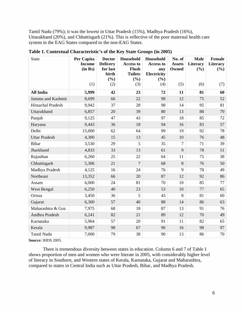
Indian states are characterized by tremendous socioeconomic diversity. Table 1 shows
some of the key characteristics of Indian states (aggregated from IHDS 2005 data). Because the
IHDS samples are not designed to be representative at state level and in case of union territories,
and north-eastern states are relatively small (Desai et al. 2009), we combine the 34 states and
union territories into 22 groups where smaller states or Union Territories are combined with
adjacent states. We present data on five indicators, average per capita income (in 2005 Rs.),
percent of doctor assisted deliveries, percent households with access to flush toilets, percent
households with access to electricity, and average number of consumer durables owned by a
household.4
The primarily urban union territory of Delhi has the highest per capita income (Rs
15,000), followed by the Northeastern States (Rs 13,350), Kerala (Rs 9,987) and Himachal
Pradesh (Rs 9,942). The poorest regions in the sample in 2005, that have the lowest per capita
income are Orissa (Rs 3,450), followed by Bihar (Rs 3,530), Madhya Pradesh (Rs 4,125), and
Uttar Pradesh (Rs 4,300). Household assets show the long-term economic standing of
households. Together, assets and amenities such as electricity depict the overall quality of life.
Column 5 in table 1 aggregates data from IHDS 2005 to the State level and we can see that
Bihar, Chhattisgarh, Orissa, Jharkhand and Madhya Pradesh are the poorest States, and Delhi,
Punjab, Haryana, and Kerala are the richest. From measures of per capita income/average
number of assets owned, all of the poorest States are “Empowered Action Group (EAG)” States
(greater explanation in section 4).
In terms of access to electricity, about 72% households in the IHDS 2005 sample had
electricity in 2005 (column 4, Table 3). States where the lowest percentage households had
access to any electricity were: Bihar (35%), Orissa (43%), Uttar Pradesh (45%, and West Bengal
(53%). Only 23% households all over India (in the sample) had access to flush toilets. There was
a wide state-wise variation in percentage households with access to flush toilets; while in Kerala
and Delhi, it was more than 60%; in some of the poor States (Bihar, Orissa and, Chhattisgarh), it
is below 10%. Finally, column (2), shows the percentage women in each state group who had a
doctor assisted delivery (for their last birth). Physician assisted delivery is an indicator of the
larger maternal care system in the state. In the IHDS 2005 sample, 42% women had a doctor
assisted delivery, however there was a large state level variation in doctor assisted deliveries.
While, it was the highest in the Southern States of Kerala (98%), Andhra Pradesh (82%) , and
4 The IHDS asked questions on the goods households owned and quality of the household (on 30 items that include:
a) ownership of goods such as television, refrigerator, chair/table etc.; and b) quality of housing (such as pucca wall,
roof, electricity etc.).
6
Tamil Nadu (79%); it was the lowest in Uttar Pradesh (15%), Madhya Pradesh (16%),
Uttarakhand (20%), and Chhattisgarh (21%). This is reflective of the poor maternal health care
system in the EAG States compared to the non-EAG States.
Table 1. Contextual Characteristic’s of the Key State Groups (in 2005)
State Per Capita
Income
(in Rs)
Doctor
Delivery
for last
birth
(%)
Household
Access to
Flush
Toilets
(%)
Household
Access to
any
Electricity
(%)
No. of
Assets
Owned
Male
Literacy
(%)
Female
Literacy
(%)
(1) (2) (3) (4) (5) (6) (7)
All India 5,999 42 23 72 11 81 60
Jammu and Kashmir 8,699 66 22 98 12 75 52
Himachal Pradesh 9,942 37 28 98 14 95 81
Uttarakhand 6,857 20 39 80 13 88 70
Punjab 9,125 47 43 97 18 85 72
Haryana 9,443 36 18 94 16 83 57
Delhi 15,000 62 64 99 19 92 78
Uttar Pradesh 4,300 15 13 45 10 76 48
Bihar 3,530 29 5 35 7 71 39
Jharkhand 4,833 33 13 61 9 78 51
Rajasthan 6,260 25 22 64 11 75 38
Chhattisgarh 5,306 21 7 68 8 76 50
Madhya Pradesh 4,125 16 24 76 9 78 49
Northeast 13,352 66 20 87 12 92 86
Assam 6,000 24 81 70 10 85 77
West Bengal 6,250 40 23 53 10 77 65
Orissa 3,450 36 5 43 8 81 60
Gujarat 6,300 57 40 88 14 86 63
Maharashtra & Goa 7,975 68 18 87 13 91 76
Andhra Pradesh 6,241 82 21 89 12 70 49
Karnataka 5,964 57 20 91 11 82 65
Kerala 9,987 98 67 90 16 98 97
Tamil Nadu 7,000 79 38 90 13 86 70
Source: IHDS 2005.
There is tremendous diversity between states in education. Column 6 and 7 of Table 1
shows proportion of men and women who were literate in 2005, with considerably higher level
of literacy in Southern, and Western states of Kerala, Karnataka, Gujarat and Maharashtra,
compared to states in Central India such as Uttar Pradesh, Bihar, and Madhya Pradesh.
7
4. Demographic Diversity in India
Socioeconomic diversity of India is also reflected in its demography. India is expected to
surpass China by 2027, to become the most populous country in the World (United Nations
Population Division, 2019). India's contribution to the yearly world population growth is higher
than that of any other country (approximately 19 million out of 89 million). As in other
developing countries, population growth in India is largely based in the poorest areas with high
populations (PRB report on Census 2011).
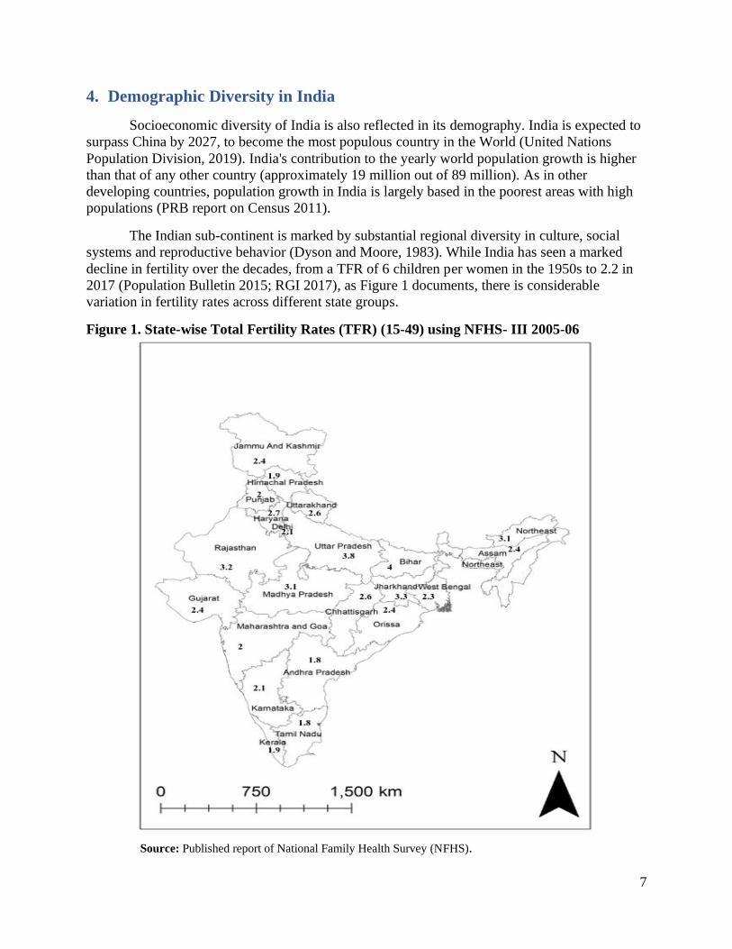
The Indian sub-continent is marked by substantial regional diversity in culture, social
systems and reproductive behavior (Dyson and Moore, 1983). While India has seen a marked
decline in fertility over the decades, from a TFR of 6 children per women in the 1950s to 2.2 in
2017 (Population Bulletin 2015; RGI 2017), as Figure 1 documents, there is considerable
variation in fertility rates across different state groups.
Figure 1. State-wise Total Fertility Rates (TFR) (15-49) using NFHS- III 2005-06
Source: Published report of National Family Health Survey (NFHS).

8
While a group of Northern States with high population, a larger prevalence of traditional
norms and beliefs, lesser educational attainment, and less effective administration termed as
“Empowered Action Group (EAG)” States (Bihar, Chhattisgarh, Jharkhand, Madhya Pradesh,
Orissa, Rajasthan, Uttarakhand, and Uttar Pradesh), accounted for 46 percent of India’s
population in 2011 and 53% of the growth in population, the Southern States comprised of 21%
of India's total population in 2011 but contributed to just 15% of the national population growth
from 2001 onwards.
Fertility rates are lower than the replacement level of 2.1 in 12 States, and union
territories. Amongst the districts, 28% of all Indian districts (174 out of 621) have a fertility level
below 2.1. It is anticipated that 12 districts all over India could achieve the lowest low fertility
rates by 2020 (Guilmoto and Rajan, 2013). On the other hand, there are 72 districts that have
fertility rates above 4. These districts are spread across the Northern and Northeastern region.
The fall in fertility in these regions in the last decade has been lower than the national average.
5. India Human Development Survey (IHDS)
This chapter relies on data from the from the first nationally representative panel data
from the India Human Development Survey (IHDS). IHDS is a nationally representative survey
of 41,554 households (includes 215,754 individuals) that are spread across all the States and
Union Territories of India (except for Andaman Nicobar and Lakshadweep), covering 384
districts, 1503 villages and 971 urban blocks. This survey was first conducted in 2005 and with
the same households being re-interviewed with an 83% re-contact rate . Survey questions
included information on income, consumption, education and morbidity experiences of various
household members.
Additionally, ever-married women aged 15-49 were interviewed in Wave 1 (2004-5)
about gender relations, fertility history, contraceptive use and number of ideal children. These
women were again interviewed in 2011-12, presenting us with a longitudinal panel in which we
can examine women’s ability to carry out their fertility preferences over a period of about 7
years. In the present study our sample is restricted to 20,464 ever married women aged 18-40 in
2005 who were interviewed in both rounds. We further restrict our focus to women aged 40 and
below to ensure that early menopause, or infecundity does not bias our results. In addition
sample size is limited (for descriptive results in Appendix Table 1, Tables 3,4), to non-missing
data for each of the dependent, independent, and control variables. Specifically for the key
dependent variables, descriptive analyses for a) ideal family size in 2005 is non-missing for
19,132 women; whereas the variable measuring b) unintended births between 2005 and 2012 is
limited to 13,128 women (for whom the number of living children in 2005 was less than or equal
to ideal family size in 2005). Finally, regression analyses presented in tables 5 and 6 is limited
only to women who had at least one birth between January 2000, and their interview date in
2005; this is because data on maternal healthcare utilization is available only for these women.
Thus, the sample size for the regression analysis in case of ideal family size as reported in 2005
is limited to 8,348 women. In addition, since the sample size for the binary outcome variable
measuring at least one unintended birth between 2005 and 2012 is further limited to only those

9
who had children less than or equal to ideal family size in 2005, the sample size for the second
regression analyses is limited to 5,903 women.5
6. Conceptual Framework for Explaining India’s Demographic Diversity
India’s demographic diversity, combined with longitudinal data, allows us to understand
the role of socioeconomic development vis-à-vis state policy, and infrastructure in shaping
fertility differentials between Indian states. Two separate processes may account for
demographic diversity between states. As Table 1 indicates, north-central states are home to
some of the poorest, and the least educated populations in India. They are also characterized by
poorly functioning public health systems. Hence, we first examine the extent to which individual
characteristics such as education, wealth, and intra-household relationships explain inter-state
differences in fertility preferences. Thereafter, we examine the extent to which these same
characteristics explain women’s ability to implement their preferences, and avoid unwanted
birth. We hypothesize that individual factors will play a greater role in explaining inter-state
variation in fertility preferences, than in explaining unplanned and possibly unwanted births. The
latter may be a function of state level public health systems, and family planning service
delivery.
Research on fertility argues that both demand for children, and ability to avoid unwanted
fertility (Bongaarts,1994) form key components of total completed fertility; with socio-economic
and ideational factors playing an important role in shaping demand for children, and
contraceptive knowledge and availability shaping unwanted fertility. Unfortunately, empirical
research often finds it difficult to distinguish neatly between the two. Demand for children,
typically measured by questions regarding ideal family size, is affected by ex post rationalization
(Lightbourne 1985; Bongaarts 1990, 2011; Westoff 1991; Bhushan and Hill 1996), i.e. ideal
family size is adjusted in a way that it is closer to actual family size (even when desired family
size is actually lower than actual family size). Consequently, measures of unwanted fertility are
typically derived at the population level rather than at individual levels, making it difficult to
examine factors driving individual women to have more children than they may consider ideal.
Using longitudinal data we are able to partially address this shortcoming, and try to
distinguish between factors that may affect ideal family size, from those that affect unwanted
fertility in subsequent years. In the present study, we focus on two indicators of fertility
preferences and subsequent behavior.
6.1. Ideal Family Size in 2005:
International (Bulatao, 1981; Bulatao & Lee, 1983; Bankole, 1995) as well as India
specific literature (Bongaarts, 2001; Dharmalingam et al., 2014) argues that demand for children
plays an important role in shaping fertility. Ideal family size is often used as an indicator of
demand for children in research focusing on India (for example Roy et al. 2008; Chatterjee and
5 In analyses not reported here, we removed the restriction women with a birth in the five years preceding the 2005
interview to expand the sample size. Our conclusions did not change. Hence, for parsimony only the final regression
results are presented on the restricted sample.

10
Kastor 2018). We measure ideal family size using the following questions, administered to
eligible women respondents at Wave 1 of the IHDS survey:
‘If you could go back to the time you did not have any children and could choose
the number of children to have in your life, how many would that be?’
This is a continuous variable that ranges from 0-12 in our data.
6.2. Undesired births between 2005 and 2012:
Unwanted fertility is far more difficult to measure due to ex-post rationalization and its
aggregate measures have led to considerable debate (Pritchett, 1994; Bongaarts, 1994). Instead
of relying on aggregate measures, we exploit longitudinal data to measure unplanned fertility. In
order to construct the measure, we use the ideal family size variable in 2005; and limit our
sample to those women who had living children fewer than, or equal to ideal family size in 2005.
As the next step, we go on to see whether these women exceeded their ideal family size as
reported in 2005 by 2012. If the total number of living children in 2012, is greater than the ideal
family size in 2005, then the binary variable measuring unplanned births takes a value of 1; and
the variable takes a value of 0 if the total number of living children as reported in 2012 is less
than or equal to ideal family size in 2005.
7. Statistical Model:
Results presented in the paper are based on the hierarchical linear models which view
individuals as being nested in within a state. Multilevel (random effects) models can be
conveniently expressed as a system of equations at separate levels (Bryk and Raudenbush 1992;
Goldstein 1995).
First, for the dependent variable measuring ideal family size in 2005, we consider a simple, two
level random intercept model,
𝒴𝒾𝒿 = 𝛽 + 𝔲𝒿(2)
+ 𝜖𝒾𝒿(1)
------------ (1)
for the measurements i (level 1 observations)= 1, 2, …..𝒏𝓳; and level 2 (state groups) j=1,
2,….,M. 𝒴𝒾𝒿 is the outcome variable: ideal family size in 2005 for the 𝒾th person in the 𝒿𝑡ℎ state,
𝛽 an unknown fixed intercept, 𝔲𝒿(2)
is a random intercept, and 𝜖𝒾𝒿(1)
is a level 1 error term. The
assumption is that the errors are distributed normally with mean 0, and variance 𝜎12 ; random
intercepts are assumed to be normally distributed with mean 0 and variance 𝜎22, and to be
independent of error terms (StataCorp LP, 2013). The interclass correlation coefficient (ICC)
denoted by 𝝆 for this model and is calculated as follows:
𝜌 = 𝐶𝑜𝑟𝑟(𝒴𝒾𝒿, 𝒴𝒾′𝒿 ) = 𝜎22/(𝜎1
2 + 𝜎22)………..(2)
In model 1 we include only state level random effects; and in models 2 and 3 we add the other
individual/household level variables of interest such as education, asset quintile, etc.; and
variables indicating a woman’s connection with the maternal and child health system (whether
she obtained any ANC or PNC) in 2005.

11
Next, going on to the second dependent variable: a binary variable indicating whether a woman
had an unintended birth between 2005 and 2012, we used mixed effects logistic regression. The
most basic equation partitions the variance in unintended births across individuals, and states is:
ln (P𝑖𝑗
1−P𝑖𝑗))= 𝛽0𝑗;-------- (3)
𝛽0𝑗 = 𝛿00 + 𝜇0𝑗
Where p𝒾𝑗 reflects the probability of ith woman in jth state having an unintended birth. The logit
of unintended birth is a function of a randomly varying state specific component 0j. The state
specific component is determined by the size of the random effects term µ0j. The ICC can be
calculated to estimate the importance of clustering in unintended births (Snijders and Bosker
2000) using the following formula:
ICC=0/(0+2/3)------ (4)
Where 0 is the estimated variance of the random effects term µ0j, and is the quantity 3.14159.
Using IHDS data, we find that without including any covariates, the ICC is 0.10. This suggests
that for unintended births, about 10% of the variance lies between states and 90% is between
women in a state. The goal is to reduce this unexplained between-state variance through
inclusion of individual, and household factors that account for compositional differences
between states.
The next step adds a series of individual and household level control variables, to take
into account the compositional differences between districts. This equation includes:
ln (P𝑖𝑗
1−P𝑖𝑗))= 𝛽0𝑗 + 𝛽1𝑗𝑋1𝑖--------(5)
Where X1i represents woman specific characteristics such as birth cohort (age), parity, and
education; and the other substantive variables of interest that are operationalized at an individual
level (e.g. household wealth). In the final model 3 we add variables indicating a woman’s
contact with the maternal and child health system.
Change in the between-state variance reflects the importance of compositional
differences across states. The above example describes our modeling strategy for the bivariate
variable, unplanned fertility.
In summary, we estimate hierarchical regression models for two dependent variables: a)
ideal family size in 2005; and b) women who have at least one unintended birth between 2005
and 2012. For each of these dependent variables, we run two sets of model: i) model 1: with only
random intercepts for state groups; and ii) model 2: model 1+ all other individual and household
characteristics (except ANC/ PNC use in 2005); and iii) model 3: model 2+ ANC and PNC use
as reported in 2005. Model 3 is indicative of a woman’s connection with the maternal and child
health system, which in turn reflects availability of maternal healthcare facilities in the region.
These hierarchical models that take into account geographical clustering at state level; and thus
regional heterogeneity is taken into account (for e.g. these models account for the fact that
women's ideal family size within states, are not independent, since women residing in different
states could have different exposure to characteristics specific to that state). All analyses is done
using Stata 15. The hierarchical models are estimated using Mixed command in STATA, and it
includes random intercepts for the state of residence. Finally, for both sets of regressions we

12
calculate the Intra-Class Correlation Coefficient (ICC) in STATA, in order to estimate the
importance of state-wise clustering in fertility intentions and behavior (Snijders and Bosker
2000; Desai and Wu 2010).
Since data on ANC/PNC is limited to women who had a child in the five years preceding
the 2005 survey, sample for model 3 is smaller than that for model 2 ( i) 8,348 compared to
19,132 for the dependent variable: ideal family size; and ii) 5,903 compared to 13,128 for the
dependent variable measuring unintended births). In order to consistently analyze changes in
ICC, we present all three models for the final smaller sample, but models estimated on the larger
sample (i.e. 13,128 and 19,132 women respectively for the two dependent variables) show
qualitatively similar results and do not affect the discussion in Section 10.6
8. Individual Level Determinants of Fertility
Our focus on examining inter-state differences in fertility relies on examining changes in
inter-state variance by adding controls for known individual level correlates of fertility
preferences and behaviors. While we control for a range of individual characteristics such as
education and household income, we also control for somewhat more distal factors that have
been hypothesized to shape both demand for children, and individuals’ ability to implement their
preferences:
8.1. Ideational Factors
Theories from sociology, psychology, cognitive sciences and communication studies
propose various processes through which people form attitudes. Some of these processes would
include socialization, processing social information, social learning and social influence. These
theories focus on structural (such as an individual's position in a given network) and ideational
(such as attitudes and beliefs of other members in a network) forces. Theories further stress on
the importance of disseminating new information and putting them in practice amongst
individuals belonging to various networks. Mead (1967) emphasized on the importance of role
taking, and interaction with network members in the shaping of an individual's self (including
his/her attitude). Various studies examine the impact of media on an individuals' development of
their behavior and self-identity (e.g. Barber and Axinn, 2004; Bennett,1975; Gamson et. al.,
1992; Gamson and Modigliani,1989).
The idea that smaller family size is preferable is often spread through various
communication networks that may or may not be a part of family planning program initiatives.
Under the thesis of ideational forces (Cleland and Wilson, 1987) empirical work may be
categorized into research on a) diffusion; b) impact of mass media and c) social interaction of
ideas about fertility and actual fertility behavior (Freedman, 1997). Bongaarts and Watkins
(1996), Watkins (1992) and Watkins et al., (1995), studied diffusion through social interactions,
in different types of natural groups. They emphasize the importance of social networks in the
dissemination of ideas on fertility, and thus in shaping fertility preferences.
6 Tables available on request from authors.

13
Studies have suggested that newspaper, radio and television campaigns lead to a rise in
available knowledge and communication on use of contraceptives and family planning issues,
declines in fertility desires and rise in use of sterilization. These relationships have been found in
contexts of various countries such as Iran, Brazil, Guatemala, Nigeria, Zambia, Columbia,
Gambia etc. (review by Hornik and McAnany, 2001).
Technological innovation, and access to effective contraception has been an important
determinant in bringing about declines in unintended pregnancy and fertility especially for those
with comparatively bigger families (Ryder 1973; Westoff 1972; Westoff and Bankole 1996). \
Barber and Axinn, 2004 examine the role of mass media (as a means of social change) that
impacts an individuals’ behavior principally through ideational mechanisms. They use data for
1091 couples in the Chitwan Valley Family Study and find that exposure to mass media is
associated with fertility behavior, inclination towards have smaller families, weaker son
preferences and greater toleration of contraceptive use.
The first demographic transition in Europe, and the ongoing fertility decline in the
developing countries can be somewhat attributable to the diffusion of new ideas and types of
contraception (Bongaarts and Watkins, 1996). When individuals communicate on new ideas
about fertility, family size, gender roles, information on experience and acceptance towards
modern contraceptives their exposure to available information and their interaction with others
impacts their attitudes towards their acceptability of high fertility and ways to restrict births
(Montgomery and Casterline 1993,1996, Kohler 2001; Kohler et al. 2001; Buhler and Kohler
2004). Qualitative research conducted in Italy and Germany show that interpersonal
communication is also seen as an important factor in determining fertility behavior (Bernadi
2003; Bernadi et al.2005).
The framework of the diffusion theory has been studied in the context of India
particularly to falls in fertility in South India. In regions where fertility decline began earlier, the
rate of diffusion was faster across social and cultural groups compared to regions where fertility
decline begun later (Guilmoto and Rajan 2001). Dommaraju and Agadjanian (2009) find that the
rate of diffusion in the Southern States was faster compared to the Northern States where it was
almost absent. Appel et. al (2002) found that in southern India diffusion of low fertility took
place across caste, religious and economic groups.
While a host of factors have been identified to promote diffusion of ideas regarding
importance of family limitation and knowledge about contraceptive use (see National Research
Council 1999), we focus on two key determinants. The first set of factors relate to the exposure
of women to mass-media and the second relates to the connection of households with formal
institutions. Role of newspapers, television and radios is often seen as key force promoting
ideational change (Faria and Potter 1999). The second set of factors identifies connections to
formal institutions. Studies (e.g. Basu and Sunder 1988) also document that social networks, and
connections to individuals who travel in the larger world and may be exposed to what has come
to be known as “developmental idealism” (Thornton et al. 2015), a complex of ideas regarding
value of delayed marriage, smaller families and use of contraception.

14
Following is a description of how we operationalize these variables:
Exposure of women in the household to mass media: The IHDS survey asks whether women in
the household were exposed to television, radio and newspaper. The response to this question
was, none, sometimes, and regularly. We recode this to, no exposure, and at least some exposure
(this combines the categories sometimes and regularly). Next, we recode the missing values on
this question, to no exposure to any form of mass media. The index for exposure of women in the
household to mass media is an additive index (ranging from 0-3), that takes a value of 0 if
women in the household have no exposure to any form of mass media, and takes a value 3 if
women in the household have at least some exposure to all 3 forms of mass media. The missing
responses were recoded to 0 (indicating no exposure to mass media). We create dummy variables
for each category of the index and take no exposure to mass media as the reference group.
Number of formal social networks: The household questionnaire in 2005 asked:
‘Do you or any members of your household have personal acquaintance with someone who
works in any of the following occupation. a) Medical profession, b) Schools, and c) Government
services.’ Each of these had a binary no (0), yes (1) response. We construct an additive index that
counts the total number of formal social networks, and ranges from 0 (no formal social networks)
to 3 (all three formal social networks). The missing responses were recoded to 0. We create
dummy variables for each category of this index, and take no formal social networks as the
reference group. A limitation of this variable is that we only look at whether the family member
knows anyone in the formal sector, but does not capture the type of the network, this is because
for a large proportion of our sample, data on type of network is missing, and we did not want to
lose those cases.
8.2. Intra-Household Bargaining Power
Research and public policies assume that women’s ability to implement their fertility
preferences is dependent upon their ability to obtain cooperation from other family members.
Past studies have found that women’s empowerment influences her fertility intentions, and her
ability to implement her intentions into actual behavior (for e.g. Upadhyay and Karasek 2012;
Kishor and Subaiya 2008, Balk 1994, Hindin 2000, Upadhyay et al. 2014). In an extensive
review article based on 60 studies examining the relationship between women’s empowerment
and fertility, Upadhyay et al. 2014, find that the most commonly used measure of women’s
empowerment was women’s role in household decision making (used in 37 of the 60 articles). In
the present study, along the lines of assumptions by Upadhyay and Karasek 2012, we assume
that, as a woman is more empowered, she will have higher aspirations for herself and her
children, which would lead to her lowering the ideal number of children she wants, and the
actual number of children she has, so that she has more resources to spend on herself and her
children. We include markers of women’s decision-making authority in the household as a
marker of gender empowerment.
Household Decision Making Ability: In the IHDS survey, eligible women in 2005 were asked
who (respondent, husband, senior male, senior female, other, or no one) had the most say in the
following household decisions: a) what to cook on a daily basis, b) whether to buy an expensive
item such as television or refrigerator) how many children to have; if they have children: d) what
to do if a child falls sick, e) whom should ones’ child marry. The response to each of these
questions takes a value of 1 if the respondent (the eligible woman) has the most say, and takes a

15
value of 0 otherwise. We recode the missing values on this question, to 0. In order to construct
this variable we look into all decisions except the decision on what to cook on a daily basis, since
this is usually a decision that is taken by women. We construct an additive index for the number
of decisions in which the respondent has the most say. This ranges from 0 (indicating that the
woman doesn’t have the most say in any of the household decisions), to 4 (indicating that the
woman has the most say in all four decisions). We create dummy variables for each category of
this index, and take most say in no decision as the reference group.
8.3. Contact with Health Systems
The next two variables measure a woman’s contact with the maternal and child health
care system, and is limited only to those who had a birth between January 2000, and the time
when she was interviewed in 2005, and had valid data on maternal healthcare utilization for their
last birth. If women have availed antenatal and postanatal check-ups in the past, it would mean
that they have had a connection with reproductive health workers in the recent past.
Antenatal checkup (ANC): This is a binary variable measuring whether a woman obtained any
antenatal checkup during her last pregnancy (as reported in 2005). It takes a value ‘1’ if a woman
obtained at least one antenatal check-up during her last pregnancy, and takes a value of ‘0’ if a
woman had obtained no antenatal checkup during her last pregnancy.
Postnatal checkup (PNC) index: This index takes a value ranging from 0 to 2. This variable
takes a value of 0 if a woman and her child obtained no postnatal check-up, a value of 1 if at
least one of them obtained a postnatal check-up, but more than 24 hours after birth but within 2
months of birth, and takes a value of 2 if at least one of them obtained a postnatal checkup within
24 hours of birth as per WHO recommendations (WHO 2014).
8.4. Socio-economic Individual and Household Characteristics
In addition to the more distal factors influencing fertility behaviors such as social
networks and exposure to mass media, we also control for some of the key socio-economic
household and individual level characteristics that have been shown in the past literature to affect
fertility. These include:
Education, parity, and age: woman’s education level (dummy variables are constructed for six
categories namely: illiterate, some primary education, primary complete, secondary complete,
higher secondary complete, and college or higher); number of living children in 2005 (parity in
2005); and age group (dummy variables are constructed for 5 age categories: 18-20, 21-25, 26-
30, 31-35, and 36-40 respectively).
Household Wealth: Household asset quintile (dummy variables are constructed for 5 categories,
ranging from the poorest to the richest households);
Caste and Religion: Caste and religion are frequently identified as primary axes along which
social intercourse as well as social stratification takes place (Desai and Dubey, 2011; Desai et al.
2010). A salient characteristic of the Hindu religion is the division into castes. This
classification is hierarchal in nature, and was historically based on occupation. Under article 341
of the Indian constitution, the lowest ranking castes are now part of an official list or schedule,
and are referred to as Scheduled Castes (SC). In a similar manner, all indigenous tribes of India

16
are part of an official schedule under article 342 of the Indian constitution, and are referred to as
Scheduled Tribes (ST). Historically both groups have lived on the margins of the mainstream
Indian society. Scheduled Tribes, often live in isolated regions where employment and
occupational opportunities as well as health services are limited. While Scheduled Castes are not
geographically isolated, they also suffer from exclusion, particularly in access to health services
(Sabharwal et al. 2014).
Hence we control for caste and religion of individuals by including indicators for caste
group (dummy variables constructed for 4 categories namely, Forward Caste groups (such as
Brahmins, Kayasthas, Kshatriyas, etc.); and lower caste groups: Scheduled Castes (SC),
Scheduled Tribes (ST), and Other Backward Classes (OBC)); and indicator for religious group
(dummy variables are created for each of the following categories: Hindu, Muslim and Other
Religions).
While an increase in education is expected to be associated with lower fertility (for e.g.
Jejeebhoy, 1995; Murthi et. al, 1995); some studies in the Indian context have shown that
Muslim women are likely to have higher fertility and lower contraception use compared to Hindu
women (for e.g. Dharmalingam and Morgan 2004; Kulkarni and Algarajan, 2005). On the other
hand the hypothesized relationship between caste and fertility is not very clear (Malhotra et al.
1995). While on one hand people belonging to lower castes are poorer, and people belonging to
poorer families will be expected to have more children in order to obtain an additional source of
labor income; on the other hand literature on social stratification indicates that ‘status’ concerns
might lead to higher fertility amongst upper caste groups (Malhotra et al. 1995; Miller 1981).
Area of residence: This is a variable with 4 different categories namely: metro cities, other urban
areas, more developed villages and less developed villages. There is a lot of variation in terms of
urban and rural areas in India. While some large Indian cities have global influence, some other
urban areas are hardly different from bigger villages (Desai et al. 2009). Therefore, the IHDS
classifies urban regions into: a) metro cities (Mumbai, Kolkata, Delhi, Chennai, Hyderabad, and
Bangalore), b) other urban areas. Similarly, rural areas are divided into two groups based on an
index of infrastructural development. Villages that have ample infrastructure (such as paved
roads, access to urban centers, postal and telephone connections, access to electricity that powers
lights and television) are coded as more developed villages; and villages that have poor
infrastructure are coded as less developed villages.
9. Descriptive Statistics
Two-child norm seems to have taken a firm hold in India. In the overall national sample,
about 1 per cent women said they didn't want any children. Figure 2 shows that 4.1% had an
ideal family size of 1, 58.9% women had an ideal family size of 2, 23.1% women had an ideal
family size of 3, and about 12.8% had an ideal family size of 4 or more.

17
Figure 2 Distribution of ideal family size in 2005 (weighted)
Sample size, n=19,132, using IHDS-1 data
Table 2 shows the distribution of ideal family size across different states. This table also
shows a strong preference for two-child families in most states. The two States that are
exceptions with respect to this are Bihar and Uttar Pradesh. In Bihar, majority women had an
ideal family size of 4 or more children (36.29%), followed by an ideal family size of 3 children
for 36.29%; whereas in Uttar Pradesh, majority women (35.42 %) had an ideal family size of 3,
and the second highest preferred family size was 2 children (for 33.92% women).
Table 2 Distribution of state-wise ideal family size in 2005# (weighted)
State 0 1 2 3 4+ Missing
All India 1.04 3.9 55.53 21.84 12.01 5.68
Jammu and Kashmir 2.31 1.36 37.7 35.32 13.16 10.14
Himachal Pradesh 0.92 15.39 76.68 4.75 1.29 0.97
Uttarakhand 0 3.58 53.35 25.55 15.16 2.36
Punjab 12.43 4.54 61.07 15.03 4.21 2.72
Haryana 0.73 1.85 61.61 23.49 1.66 10.65
Delhi 0.41 0.38 71.17 17.43 6.49 4.12
Uttar Pradesh 1.23 1.56 33.92 35.42 21.57 6.29
Bihar 0 2.79 22.05 35.93 36.29 2.93
Jharkhand 0 1.35 43.53 35.1 17.07 2.94
Rajasthan 0.39 1.91 61.99 22.51 6.7 6.51
Chhattisgarh 0 0.55 53.03 32.68 8.38 5.36
Madhya Pradesh 0.06 0.96 57.99 20.88 16.85 3.25
Northeast 1.43 9.65 42.37 9.11 22.66 14.78
Assam 2.22 0.61 39.65 26.22 11.59 19.71
West Bengal 0.63 11.59 68.54 9.35 3.61 6.28
0
1%
1
4%
2
59%
3
23%
4 and more
13%

18
State 0 1 2 3 4+ Missing
Orissa 0 4.71 62.2 21.01 8.2 3.88
Gujarat 0.24 4.27 72.22 14.97 0.77 7.54
Maharashtra & Goa 0.52 2.59 61.5 17.44 10.62 7.33
Andhra Pradesh 1.71 4.03 65.35 19.71 4.87 4.34
Karnataka 3.61 3.68 67.15 10.11 8.79 6.66
Kerala 0.29 3.48 71.26 14.1 4.65 6.21
Tamil Nadu 0.5 8.98 75.75 8.32 3.68 2.77
#Indicates proportion with ideal family size 0,1,2,3,4 and more, across States.
n=20,464
Table 3 shows average ideal family size in 2005 (column 1), and the percentage women,
who had at least one unintended birth between 2005, and 2012 (column 2) across 22 state groups.
The average ideal family size in 2005 in India was 2.45, the average in EAG states was higher
than the all India average at 2.74, while the average ideal family size for non-EAG states was
lower (2.21) than the all India average. While looking separately at the 22 States, it can be seen
that average ideal family size in 2005, was greater than the all India average in the States of
Jammu and Kashmir, Uttarakhand, Uttar Pradesh, Bihar, Jharkhand, Chhattisgarh, Madhya
Pradesh, Assam and other Northeastern States. There was only one state: Bihar (3.18),where
average ideal family size in 2005 was above 3 children.
Table 3 Ideal family size in 2005 and Unintended Births between 2005 and 2012*
State Average Ideal
Family size
Percentage women who have
atleast one unintended birth
between 2005 and 2012+
TFR 2005-
06
(1) (2) (3)
All India 2.45 17.56 2.7
EAG States 2.74 25.42 3.1
Non-EAG States 2.21 11.7 2.4
Jammu and Kashmir 2.64 14.8 2.4
Himachal Pradesh 1.9 23.33 1.9
Uttarakhand 2.57 36.61 2.6
Punjab 1.95 15.39 2
Haryana 2.26 22.97 2.7
Delhi 2.31 29.28 2.1
Uttar Pradesh 2.85 23.99 3.8
Bihar 3.18 33.51 4
Jharkhand 2.74 25.42 3.3
Rajasthan 2.37 23.98 3.2
Chhattisgarh 2.54 20.74 2.6
Madhya Pradesh 2.57 23.03 3.1
Northeast 2.67 15.05 3.1

19
State Average Ideal
Family size
Percentage women who have
atleast one unintended birth
between 2005 and 2012+
TFR 2005-
06
(1) (2) (3)
Assam 2.57 13.78 2.4
West Bengal 2.04 14.76 2.3
Orissa 2.34 17.66 2.4
Gujarat 2.13 23.38 2.4
Maharashtra & Goa 2.39 10.74 2
Andhra Pradesh 2.24 8.57 1.8
Karnataka 2.2 9.73 2.1
Kerala 2.22 3.75 1.9
Tamil Nadu 2.06 4.5 1.8
Sample Size 19,132 13,128
* Calculations for columns (1) and (2) based on data for ever-married women aged 18-40 from IHDS 2005, and
2012. TFRs reported in column (3) come from National Family Health Survey III, 2005-06 report for women aged
15-49. Average TFR for EAG and non-EAG States based on State-groups used from NFHS.
Column 2 in Table 3 shows the state-wise distribution of the percentage women who had
at least one unintended birth between 2005 and 2012. As mentioned earlier, this is limited to a
smaller sample size of 13,128 women, who had children less than or equal to ideal family size in
2005. We find that almost 18% of women in this sample had at least one unintended birth
between 2005 and 2012, i.e. exceeded ideal family size as expressed in Wave 1 interview. The
percentage of women who had unintended births was much higher in EAG States (more than
25%), and lower in non-EAG States (almost 12%) compared to the national average. Proportion
of women who had at least one unintended births between 2005 and 2012 were the lowest in
Kerala (less than 4%), followed by Tamil Nadu (less than 5%), Andhra Pradesh (less than 9%),
and Karnataka (less than 10%); and the highest in Uttarakhand (36.6%), followed by Bihar
(33.5%), Delhi (29.3%), Jharkhand (25.4%), and Uttar Pradesh (24%). It is important to
remember, that the IHDS is not designed to be representative at the state level and small samples
render state-wise ranking indicative rather than definitive. Column 3 in Table 3 shows the total
fertility rates (TFR) for women aged 15-49 aggregated from National Family Survey (NFHS III,
2005-06) report, and as depicted in figure 1.
Summary statistics for the independent variables in this analysis are presented in
Appendix Table 1. We present the distribution of our two primary fertility outcomes, desired
fertility, and unplanned fertility across different independent variables in Table 4. Bivariate
statistics show a wide variation in fertility intentions (column 1), and behavior (column 2) across
education levels, income, area of residence, number of decisions in which a woman has the most
say, exposure to mass media, any connection to formal social networks, and maternal health care
utilization during the last birth, as reported in 2005.

20
Table 4 Distribution of indicators of Fertility intentions and behavior by key independent
variables (%)
Ideal
Family size
in 2005
Has an unintended
birth between 2005
and 2012+
(1) (2)
Education in 2005
Illiterate 2.69 20.95
Pre Primary 2.45 16.61
Primary 2.27 17.41
Secondary 2.1 10.83
High Secondary 2.07 11.21
College 1.92 8.96
Asset Quintile
Poorest 2.82 24.22
Second Quintile 2.66 21.72
Third Quintile 2.4 17.8
Fourth Quintile 2.25 13.57
Richest 2.1 10.91
Area of Residence
Metro Cities 2.07 10.81
Other Urban 2.25 14.22
More Developed Villages 2.4 14.52
Less Developed Village 2.63 22.7
Number of decisions in the household where the woman has the most say
0 2.48 18.84
1 2.45 17.28
2 2.28 12.69
3 2.38 15.17
4 2.33 8
Number of Social Networks in the Formal Sector
0 2.47 18.67
1 2.47 16.26
2 2.47 18.7
3 2.34 15.09
Score on Exposure to Mass media
0 2.73 23.95
1 2.45 16.95
2 2.34 16.42
3 2.17 11.12
Any ANC during the last birth#
Yes 2.35 23.89
No 3.04 39.11

21
Ideal
Family size
in 2005
Has an unintended
birth between 2005
and 2012+
(1) (2)
Postnatal Checkup during last birth#
No Postnatal check-up 2.66 29.83
First check-up after 24 hours of birth 2.26 21.92
First check-up within 24 hours of birth 2.29 23.93 # Limited to those who have a birth between Jan 2000-interview date in 2005
+ Limited to those who had children less than, or equal to ideal family size in 2005.
It can be seen that ideal family size in 2005 (column 1) decreases with an increase in
education, and is the highest for illiterate women (about 2.7), and the lowest for college educated
women (below 2). Column (2) shows that while only about 9% women with college education
have at least one unintended birth, almost 21% women who are illiterate have at least one
unintended birth. A similar pattern is observed by household socio-economic status. The ideal
family size decreases with an increase in household assets, while for women belonging to
poorest families ideal family size is 2.8, for women belonging to richest families it is 2.1.
Percentage women having an unintended birth decrease significantly as household wealth
increases. While more than 24% women belonging to poorest households have at least one
unintended birth between 2005 and 2012; less than 11 % women belonging to the richest
households have at least one unintended birth.
Differences in ideal family size across areas of residence, show that ideal family size is
highest in less developed villages (2.6), followed by more developed villages ( 2.4), other urban
areas (2.3), and lowest in metro cities (2.1). Percentage women having at least one unintended
birth, is the highest in less developed villages (almost 23%), and the lowest in metro cities (less
than 11%).
Next we look at the relationship between the number of decisions in which women
relatively have the most say, and fertility intentions and behavior. Women who do not have the
most say in any household decisions have the highest average ideal family size in 2005,
compared to women who have the most say in all 4 major household decisions. A greater
percentage of women who didn't have the most say in any household decision were likely to
have an unintended birth between 2005 and 2012, compared to women who had the most say in
all 4 household decisions.
Both ideal family size in 2005, and percentage women who had unintended births
between 2005 and 2012 did not vary much by the number of social networks in the formal
sector; though those who had connections with all three social networks had a lower ideal family
size; and also a smaller percentage of women with all three social networks had unintended
births, compared to those with no connections in the formal sector.
Ideal family size in 2005 is higher on an average for women who reside in households
that have exposure to fewer forms of mass media. Percentage women having unintended births
between 2005 and 2012 is also higher if women reside in households that have no exposure to
mass media (about 24%), compared to women who reside in households where women have
exposure to all forms of mass media (about 11%).

22
Finally, variables measuring exposure to maternal healthcare utilization during the last
birth are indicative of connectivity with the maternal and child health system, and thus the
availability of healthcare facilities in the region of residence. Women who had obtained at least
one ANC during her last birth (as reported in 2005), was likely to have a lower average ideal
family size in 2005 (2.4), compared to women who received no ANC (3) during her last birth. A
larger percentage of women who didn't receive any ANC during their last birth were likely to
have at least one unintended birth (more than 39%), compared to those who received at least one
checkup (about 24%). Similarly, for PNC use during the last birth (as reported in 2005), average
ideal family size in 2005 was lower for women who received any postnatal checkup, compared
to those who did not. Also, a higher percentage of women didn’t obtain any postnatal checkup
during their last birth (as reported in 2005) were likely to have at least one unintended birth
between 2005 and 2012.
10. Results from Multi-level Regressions
Results from hierarchical multi-level regressions are presented in Tables 5 and 6. Each
table contains three columns. Column 1 includes only state-level variation at the second level
without any independent variables; column 2 adds individual level correlates of fertility
preferences, and behaviors; and column 3 adds contact with health services for antenatal and post
natal care.
As the discussion of statistical models in section 7 notes, this approach allows us to
partition the variance into two components, within and between states. The Intraclass Correlation
Coefficient describes the component of variance that can be attributed to between state variance.
In as much as between state differences are a function of individual characteristics such as
education and economic status, addition of these factors should reduce the size of ICC between
models 1, 2 and 3.
10.1. Desired Family Size.
Table 5 shows the results from the hierarchical linear regression model for the family size
women would have wanted had they been able to choose their family at the start of their
reproductive career. This variable was reported at Wave 1 interview in 2005. Model 1 is the
basic model without any individual/household level predictors. This model enables us to obtain
the baseline ICC, with the goal of decreasing it's magnitude upon adding other individual and
household variables (in model 2), and variables indicative of maternal healthcare utilization
(model 3). ICC of 0.13 in model 1 suggests that 13% of the variation in ideal family size in 2005
is between states, and 87% of the variation in ideal family size in 2005 is between women
residing in the same state. Model 2 adds the individual, and household level independent, and
other control variables to model 1. Note that the within state component includes both systematic
variation between women based on their education, economic status, social networks and a host
of other individual characteristics identified in the literature reviewed above as determinants of
fertility preferences as well an unmeasured component reflecting idiosyncratic variation between
individuals. Adding individual /household level factors reduces the ICC from about 0.13 to 0.09,
which indicates a 35% decline between model 1 and 2. This means that a substantial part of the
inter-state variation in ideal family size is explained by the variables included in model 2. In

23
Model 3, we add contact with the health system during prior delivery. Addition of these variables
reduces the ICC to 0.08, which indicates a 39% decline from the null model. Thus, individual
and household level factors; and connection that women have with maternal and child health
workers explains a significant part of inter-state variation in ideal family size.
Table 5 Beta coefficients from hierarchical linear regression examining women's ideal
number of children in 2005
Model 1 Model 2 Model 3
Education (Reference group: Illiterate)
Incomplete primary -0.037 -0.030
(0.0341) (0.0341)
Primary -0.124*** -0.113***
(0.0226) (0.0226)
Secondary -0.162*** -0.149***
(0.0347) (0.0347)
Higher secondary -0.135** -0.119**
(0.0440) (0.0440)
College and higher -0.179*** -0.166***
(0.0498) (0.0498)
Asset Quintile(Reference group: Poorest)
Second quintile -0.110*** -0.103***
(0.0268) (0.0268)
Third quintile -0.186*** -0.172***
(0.0293) (0.0293)
Fourth quintile -0.241*** -0.222***
(0.0343) (0.0344)
Richest -0.231*** -0.208***
(0.0416) (0.0417)
Area of Residence(Reference group:Metro Cities)
Other Urban 0.019 0.029
(0.0470) (0.0469)
More Developed Villages 0.059 0.064
(0.0475) (0.0474)
Less Developed Village 0.134** 0.135**
(0.0481) (0.0480)
Religion(Reference group:Hindu)
Muslim 0.353*** 0.356***
(0.0274) (0.0274)
Other Religion 0.114** 0.120**
(0.0395) (0.0395)
Caste Group(Reference group: Forward Caste Groups)
Scheduled Castes (SC) 0.036 0.036
(0.0260) (0.0260)
Scheduled Tribes (ST) 0.253*** 0.241***
(0.0368) (0.0368)
Other Backward Classes (OBC) 0.067** 0.065**
(0.0223) (0.0222)

24
Model 1 Model 2 Model 3
Number of living children 0.218*** 0.213***
(0.0102) (0.0102)
Age Category(Reference group: 18-20)
21-25 -0.084* -0.083*
(0.0328) (0.0328)
26-30 -0.122*** -0.120***
(0.0363) (0.0363)
31-36 -0.045 -0.044
(0.0383) (0.0382)
36-40 0.021 0.016
(0.0476) (0.0476)
Number of household decisions where the woman has most say
(Reference Group: no decisions)
1 -0.046* -0.045*
(0.0204) (0.0203)
2 -0.092** -0.090**
(0.0324) (0.0324)
3 -0.094 -0.090
(0.0600) (0.0599)
4 -0.045 -0.027
(0.0617) (0.0617)
Number of formal social networks(Reference Group: no connection)
1 0.033 0.035
(0.0221) (0.0221)
2 0.005 0.005
(0.0252) (0.0252)
3 -0.077** -0.076**
(0.0272) (0.0272)
Exposure of women in to household to mass media
(Reference Group: no exposure)
1 -0.002 0.002
(0.0234) (0.0233)
2 -0.013 -0.009
(0.0265) (0.0265)
3 0.004 0.009
(0.0353) (0.0353)
Any antenatal check-up -0.111***
(0.0236)
Postnatal Checkup (Reference Group: No post natal checkup)
First check-up after 24 hours of birth -0.028
(0.0221)
First check-up within 24 hours of birth -0.075**
(0.0267)
Constant 2.411*** 2.047*** 2.136***
(0.0694) (0.0807) (0.0814)

25
Model 1 Model 2 Model 3
Random effects Parameters
Constant (level 2 State of Residence)) -1.137*** -1.485*** -1.517***
(0.1540) (0.1572) (0.1580)
Constant (residual) -0.191*** -0.297*** -0.299***
(0.0077) (0.0077) (0.0077)
ICC 0.131 0.085 0.08
Observations 8,348 8,348 8,348
Number of State Groups 22 22 22 Standard errors in parentheses
*** p<0.001, ** p<0.01, * p<0.05, + p<0.10
Results from model 2 show that, of key socio-economic and demographic variables;
being illiterate (compared to having primary or higher level education); belonging to poorest
households (compared to that for richer households); belonging to Muslim and other religious
groups (compared to Hindu groups); residing in a less developed village (compared to a metro
city); belonging to ST and OBC caste groups (compared to forward caste groups); having a
higher number of living children; and being 18-20 (compared to being 21-30 is associated with
having higher ideal family size in 2005. Having three formal social networks (compared to no
social networks in the formal sector), and, having the most say in more number of household
decisions (having the most say in one or two decisions compared to not having the most say in
any decision) is linked to having smaller ideal family size. Finally, in model 3 ANC, and PNC
use in 2005 are added to model 2, while the significance level and directions for all other
independent and control variables remain similar to that in model 2, model 3 shows that
obtaining at least one ANC (compared to obtaining none), and the first PNC within 24 hours of
birth (compared to obtaining none), during the last birth is associated with having a smaller ideal
family size.
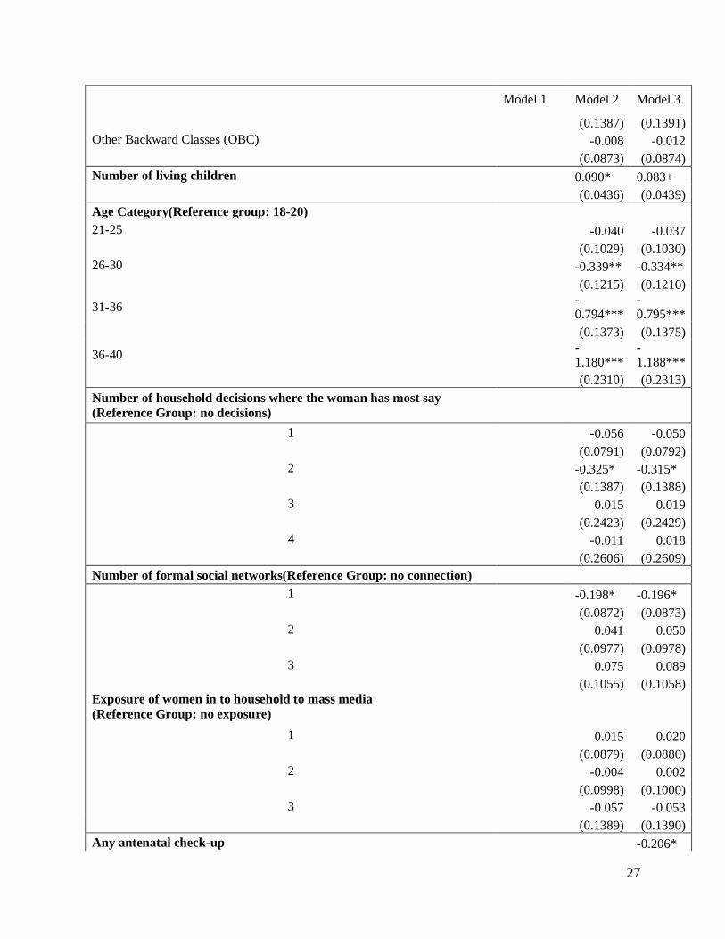
10.2. Unplanned Birth
Table 6 shows the results from the hierarchical logistic regression model examining the
likelihoods of having at least one unintended birth between 2005 and 2012. Model 1 is the basic
model without any individual/household level predictors. ICC of about 0.10 in this model.7
Adding individual, and household level variables in model 2, reduces the variance of the random
effects coefficient and reduced the ICC from 0.101 to 0.095 i.e. about 6% decline between model
1 and model 2. Adding the ANC, and PNC use variables in model 3, reduces the variance of the
random effects coefficients and reduced the ICC to 0.092, a 9% decline from the null model.
Comparison of changes in ICC between the two dependent variables, desired fertility and
unplanned births is striking. Whereas a vast proportion of inter-state variation in desired fertility
appears to be related to differing composition of women living in these states, the same cannot
7 Interpretation of ICC for logistic regressions is not strictly comparable to the one for multilevel linear models
continuous since it depends on the prevalence of outcome in clusters of interest. Furthermore, the between‐cluster
variance is defined on a different scale (e.g., the log‐odds scale in a logistic regression), than the binary response
scale (Austin and Merlo 2017).

26
be said of unintended fertility. This is more evident as we look at the variation in unintended
fertility between women with different characteristics.
Table 6 Beta coefficients from hierarchical logistic regression examining likelihoods of a
woman having at least one unwanted birth++
Model 1 Model 2 Model 3
Education (Reference group: Illiterate)
Incomplete primary -0.124 -0.117
(0.1303) (0.1304)
Primary -0.127 -0.109
(0.0844) (0.0848)
Secondary -0.171 -0.158
(0.1327) (0.1331)
Higher secondary -0.258 -0.239
(0.1731) (0.1737)
College and higher -0.465* -0.448*
(0.2085) (0.2089)
Asset Quintile (Reference group: Poorest)
Second quintile -0.074 -0.066
(0.0999) (0.1001)
Third quintile -0.199+ -0.186+
(0.1109) (0.1117)
Fourth quintile -0.376** -0.354**
(0.1321) (0.1331)
Richest -
0.576***
-
0.554***
(0.1637) (0.1648)
Area of Residence (Reference group: Metro Cities)
Other Urban -0.152 -0.138
(0.1956) (0.1958)
More Developed Villages -0.343+ -0.335+
(0.1969) (0.1970)
Less Developed Village -0.239 -0.235
(0.1981) (0.1982)
Religion (Reference group: Hindu)
Muslim 0.676*** 0.682***
(0.1044) (0.1045)
Other Religion 0.127 0.130
(0.1504) (0.1503)
Caste Group (Reference group: Forward Caste Groups)
Scheduled Castes (SC) 0.371*** 0.370***
(0.0990) (0.0991)
Scheduled Tribes (ST) 0.309* 0.297*
27
Model 1 Model 2 Model 3
(0.1387) (0.1391)
Other Backward Classes (OBC) -0.008 -0.012
(0.0873) (0.0874)
Number of living children 0.090* 0.083+
(0.0436) (0.0439)
Age Category(Reference group: 18-20)
21-25 -0.040 -0.037
(0.1029) (0.1030)
26-30 -0.339** -0.334**
(0.1215) (0.1216)
31-36 -0.794***
-0.795***
(0.1373) (0.1375)
36-40 -
1.180***
-
1.188***
(0.2310) (0.2313)
Number of household decisions where the woman has most say
(Reference Group: no decisions)
1 -0.056 -0.050
(0.0791) (0.0792)
2 -0.325* -0.315*
(0.1387) (0.1388)
3 0.015 0.019
(0.2423) (0.2429)
4 -0.011 0.018
(0.2606) (0.2609)
Number of formal social networks(Reference Group: no connection)
1 -0.198* -0.196*
(0.0872) (0.0873)
2 0.041 0.050
(0.0977) (0.0978)
3 0.075 0.089
(0.1055) (0.1058)
Exposure of women in to household to mass media
(Reference Group: no exposure)
1 0.015 0.020
(0.0879) (0.0880)
2 -0.004 0.002
(0.0998) (0.1000)
3 -0.057 -0.053
(0.1389) (0.1390)
Any antenatal check-up -0.206*

28
Model 1 Model 2 Model 3
(0.0884)
Postnatal Checkup (Reference Group: No post natal checkup)
First check-up after 24 hours of birth -0.030
(0.0868)
First check-up within 24 hours of birth 0.109
(0.1024)
Constant -1.155*** -0.613* -0.481+
(0.1354) (0.2789) (0.2851)
Random effects Parameters
Var(_Constant (level 2 State of Residence)) 0.369** 0.345** 0.332**
(0.1258) (0.1216) (0.1187)
ICC 0.101 0.095 0.092
Observations 5,903 5,903 5,903
Number of State Groups 22 22 22 Standard errors in parentheses
*** p<0.001, ** p<0.01, * p<0.05, + p<0.10
++ Limited to those who had children less than or equal to ideal family size in 2005, and those who had at least one
birth between Jan 2000 and interview date in 2005. The dependent variable measure whether these women exceed
their ideal family size in 2005, and go on to have at least one unwanted birth between 2005 and 2012.
Results from model 2 show that while education, and income reduce the likelihood of
having unplanned births, women need to reach very high levels of education or income before
this effect is large enough to be significant. Whereas for desired fertility, even a small amount of
education has a large and significant effect, for unplanned births, college education is required
before we see any impact. Similarly, there is only a small reduction in likelihood of unplanned
births between women in the bottom 60 percent of household wealth index.
Age, however, appears to have an interesting relationship with unplanned births. Younger
women seem to be particularly susceptible to experiencing unplanned birth. Since they are also
most likely to desire smaller families, this is clearly a niche where unmet need for contraception
appears to be the greatest. Unplanned births appear to be higher among Muslim, Scheduled Caste
and Scheduled Tribe households, identifying another population that seem to be poorly served by
existing service delivery infrastructure. Among other factors we control for, having no
connections in the formal sector (compared to having one connection), and having the most say
in no household decisions (compared to having the most say in a couple of household decisions)
is associated with greater likelihoods of at least one unintended birth between 2005 and 2012.
Results from model 3 add variables indicating a woman’s connection with the maternal and child
health system. Results from model 3 show that obtaining at least one antenatal checkup during
their last birth (as reported in 2005) is associated with lower likelihoods of unintended birth
between 2005 and 2012.

29
11. Discussion and Conclusion
This chapter has examined regional differences in fertility in India through the prism of
desired and unintended fertility using prospective data. Descriptive statistics presented in Table 3
show tremendous variation between states. Whereas Southern state of Karnataka had desired
family size of 2.2 children with less than 10% women having an unintended birth, Bihar in
Northern India had desired fertility of 3.18 with about a third of the women reporting unintended
birth. While these results highlight well established regional differences in fertility with states in
the Hindi speaking heartland of India showing greatest desired as well as unintended fertility,
they also shed interesting light on possible processes through which these differences emerge.
States in India are almost like mini nations, they differ tremendously in social, political
and economic culture and have tremendous independence in running their health programs. Even
when central government pays for some the major schemes such as maternal protection schemes,
its operation is left to states creating very different service delivery climate with some states able
to efficiently administer these schemes and others being lackadaisical in their governance.
Our results suggest that a substantial proportion of variation in fertility preferences
between states can be explained by individual factors such as education, and income. Poorer
states with less educated populations such as, Bihar and Uttar Pradesh have higher desired family
size. Almost 40 percent of inter-state variation in fertility preferences is reduced once we take
into account differences in these individual attributes. However, this same, well established
pathway to reduced fertility does not apply easily to unintended fertility. Education, and income
reduce unintended births, but only after they reach a very high threshold. Whereas, even
secondary enrolment reduces desired family size, it requires college education to make a
significant dent in the likelihood of unintended births. This lack of association at individual level
translates into the fact that between state variance in unintended births remains impervious to
addition of individual variables with only 9 percent decline in between-state ICC.
This suggests that the unobserved component of interstate variance is very strong, and not
easily explainable through individual factors. Some of this could be attributed to the exclusion of
socio-cultural differences across regions such as differences in kinship patterns, extent of
coresidence with parents, and gender relations (Desai et al. 2010; Dyson and Moore 1983). It is
also possible that regional differences in the quality of family planning services may result in
large inter-state variation. Although we tried to capture state provision of health services through
variables that capture use of antenatal and postnatal care, addition of these variables do not seem
to make a dent in interstate variance. We argue that this is because the measures of service
delivery we have access to are focused on maternal and child health services and may be quite
distinct from provision of family planning services. While the same health workers are supposed
to provide maternal and child health services as well as family planning services, these are two
distinct activities and it is not possible to assume that the providers who prioritize one activity
will also prioritize the other.
Our results also highlight two types of populations that seem to most at risk of having
unintended fertility. Young women below 25 have a preference for having smaller families, but
they also seem to be most at risk of being unable to implement their preferences. Muslims,
Scheduled Castes, and Scheduled Tribes also seem to be most at risk of having unintended
30
births. These observations identify niche populations that may be most at risk of being excluded
from the service delivery systems may require special programming.
At a broader level, these results document an interesting puzzle. Individual factors that
have been long established in fertility research, education, economic status, gender relations in
the household and social networks, seem to play an important role in shaping fertility
preferences. However, our ability to predict unintended fertility seems to be far more limited.
Even education, the greatest weapon in the armory of demographic research, seems to be only
weakly correlated with unintended births. This should be an important area of future research.
It is important to note possible limitations of this analysis as we interpret the results.
Firstly, for measuring fertility preferences we use ‘ideal family size’ as the key dependent
variable, this measure could be subject to ex-post rationalization, whereby women adjust their
ideal family size to be near their actual family size, which causes an overestimation of wanted
fertility (for e.g. Bongaarts, 1990,2011; Bhushan and Hill, 1995; Lightbourne, 1985; Westoff,
1991). However, by limiting our sample to those who had children lower than, or equal to ideal
family size in 2005; and subsequently checking whether this sub-group of women had more
number of living children in 2012, than their ideal family size in 2005, enables us to partially
address this limitation. Secondly, we have assumed that fertility preferences as expressed at
Wave 1 interview reflect long term predisposition on the part of individuals towards having a
particular number of children and taken deviation from over the subsequent eight years as
unintended fertility. However, individuals may have adjusted their fertility preferences upwards,
and what we define as unintended fertility may well reflect a change in preference rather than
inability to implement preferences. In spite of this caveat, we suggest that longitudinal data on
preferences and their implementation provide us with a way of looking at regional differences in
fertility that has not been feasible to date with cross-sectional data and deserves further attention.
In conclusion, our study uses data from the first nationally representative panel survey in
India, and examines factors that impact regional differences in fertility preferences, and on the
ability to crystallize these preferences. Results highlight that while socio-economic traits of
individuals and their household’s account for a significant portion of regional differentials in
fertility preferences, they account for a much smaller proportion of differentials in unintended
births across regions. Our study implies that unobserved factors such as cultural norms, social
structure, and particularly the quality of regional healthcare systems could play a much bigger
part in explaining differences in unintended births compared to fertility preferences.

31
References
Agadjanian, V. (2005). Fraught with ambivalence: Reproductive intentions and contraceptive
choices in a sub-Saharan fertility transition. Population Research and Policy
Review, 24(6), 617-645.
Austin, P. C., & Merlo, J. (2017). Intermediate and advanced topics in multilevel logistic
regression analysis. Statistics in medicine, 36(20), 3257–3277.
Bocquet-Appel, J. P., Rajan, I. S., Bacro, J. N., & Lajaunie, C. (2002). The onset of India's
fertility transition. European Journal of Population/Revue européenne de
Démographie, 18(3), 211-232.
Balk, D. (1994). Individual and community aspects of women's status and fertility in rural
Bangladesh. Population Studies, 48(1), 21-45.
Bankole, A. (1995). Desired fertility and fertility behaviour among the Yoruba of Nigeria: a
study of couple preferences and subsequent fertility. Population Studies, 49(2), 317-328.
Barber, J. S., & Axinn, W. G. (2004). New ideas and fertility limitation: The role of mass
media. Journal of marriage and family, 66(5), 1180-1200.
Basu, A., & Sundar, R. (1988). The Domestic Servant as Family Planning Innovator: An Indian
Case Study. Studies in Family Planning, 19(5), 292-298.
Bennett, W. L. (1975). The political mind and the political environment: An investigation of
public opinion and political consciousness (pp. 4-25). Lexington, MA: Lexington Books.
Bernardi, L. (2003). Channels of social influence on reproduction. Population research and
policy review, 22(5-6), 427-555.
Bernardi, L., von der Lippe, H., & Keim, S. (2005). Mapping social influence on fertility: a mix-
method approach to data collection. Max Planck Institute for Demographic Research
(Working Paper 2005–015).
Bongaarts, J. (1978). A framework for analyzing the proximate determinants of
fertility. Population and development review, 105-132.
Bongaarts, J. (1990). The measurement of wanted fertility. Population and development review,
487-506.
Bongaarts, J. (1994). Population policy options in the developing world. Science, 263(5148),
771-776.
Bongaarts, J., & Watkins, S. C. (1996). Social interactions and contemporary fertility
transitions. Population and development review, 639-682.
Bongaarts, J. (2001). Fertility and reproductive preferences in post-transitional
societies. Population and development review, 27, 260-281.
Bongaarts, J. (2011). Can family planning programs reduce high desired family size in sub-
Saharan Africa?. International perspectives on sexual and reproductive health, 37(4),
209-216.
Bulatao, R. A. (1981). Values and disvalues of children in successive childbearing
decisions. Demography, 18(1), 1-25.
Bulatao RA, Lee. RD, eds. 1983. Determinants of Fertility in Developing Countries. 2 vols. New
York: National Academy Press.
Bühler, C., & Kohler, HP (2004). The influence of strong ties on the use of modern
contraceptives in Kenya. Journal of Sociology , 33 (1), 5-25.

32
Campbell-White, A., Merrick, T. W., & Yazbeck, A. S. (2006). Reproductive health--the missing
Millennium Development Goal: poverty, health, and development in a changing world.
The World Bank.
Chatterjee, S., & Kastor, A. (2018). To what extent do couples’pre-marital communications
affect their post-marital fertility behaviour in india?. Journal of biosocial science, 50(4),
435-450.
Cleland, J., & Wilson, C. (1987). Demand theories of the fertility transition: An iconoclastic
view. Population studies, 41(1), 5-30.
Desai, Sonalde, and Amaresh Dubey. 2011. 'Caste in 21st Century India: Competing Narratives',
Economic and Political Weekly, 46: 40-49.
Desai, S., Dubey, A., Joshi, B. L., Sen, M., Shariff, A., & Vanneman, R. (2009). India human
development survey: Design and data quality. IHDS technical paper, 1.
Desai, S. B., Dubey, A., Joshi, B. L., Sen, M., Shariff, A., & Vanneman, R. (2010). Human
development in India. New York: Oxford University.
Desai, S., & Wu, L. (2010). Structured inequalities—factors associated with spatial disparities in
maternity care in India. Margin: The Journal of Applied Economic Research, 4(3), 293-
319.
Dharmalingam, A., & Morgan, S. P. (2004). Pervasive Muslim-Hindu fertility differences in
India. Demography, 41(3), 529-545.
Dharmalingam, A., Rajan, S., & Morgan, S. P. (2014). “The determinants of low fertility in
India.” Demography, 51(4), 1451-1475.
Dommaraju, P., & Agadjanian, V. (2009). India’s North–South divide and theories of fertility
change. Journal of Population Research, 26(3), 249..
Drèze, J., & Sen, A. (2013). An uncertain glory: India and its contradictions. Princeton
University Press.
Dyson, T., & Moore, M. (1983). On kinship structure, female autonomy, and demographic
behavior in India. Population and development review, 35-60.
Easterlin, R. A. (1978). The economics and sociology of fertility: A synthesis. Center for
Advanced Study in the Behavioral Sciences.
Easterlin, R. A. (1983). Modernization and fertility: a critical essay. Determinants of fertility in
developing countries, 2, 562-586.
Easterlin, R. A., & Crimmins, E. M. (1985). The fertility revolution: A supply-demand analysis.
University of Chicago Press.
Edin, K., & Kefalas, M. (2011). Promises I can keep: Why poor women put motherhood before
marriage. Univ of California Press.
Faria, V. E. & Potter, J. E. (1999). “Television, telenovelas and fertility change in north-east
Brazil,” in Leete, Richard (ed.) Dynamics of Values in Fertility Change (Pp. 252-274)
New York: Oxford University Press.
England, P., Caudillo, M. L., Littlejohn, K., Bass, B. C., & Reed, J. (2016). Why do young,
unmarried women who do not want to get pregnant contracept inconsistently? Mixed-
method evidence for the role of efficacy. Socius, 2, 2378023116629464.
Freedman, R. (1997). Do family planning programs affect fertility preferences? A literature
review. Studies in family Planning, 1-13.
Gamson, W. A., Croteau, D., Hoynes, W., & Sasson, T. (1992). Media images and the social
construction of reality. Annual review of sociology, 18(1), 373-393.

33
Gamson, W. A., & Modigliani, A. (1989). Media discourse and public opinion on nuclear power:
A constructionist approach. American journal of sociology, 95(1), 1-37.
Guilmoto, C. Z., & Rajan, S. I. (2001). Spatial patterns of fertility transition in Indian
districts. Population and development review, 27(4), 713-738.
Guilmoto, C. Z., & Rajan, S. I. (2013). Fertility at the district level in India: Lessons from the
2011 census. Economic and Political weekly, 59-70.
Hayford, S. R., & Agadjanian, V. (2012). “From desires to behavior: Moderating factors in a
fertility transition.” Demographic research, 26, 511.
Hindin, M. J. (2000). Women's autonomy, women's status and fertility-related behavior in
Zimbabwe. Population Research and Policy Review, 19(3), 255-282.
Hirschman, C. (1994). Why fertility changes. Annual review of sociology, 20(1), 203-233.
Hornik, R., & McAnany, E. (2001). Mass media and fertility change. Diffusion processes and
fertility transition: Selected perspectives, 208, 239.
Islam, M. M. & Bairagi, R. (2003) “Fertility intentions and subsequent behaviour in Matlab. Do
fertility intentions matter?” Journal of Biosocial Science 35, 615–619.
Jejeebhoy, S. J. (1995). Women's education, autonomy, and reproductive behaviour: Experience
from developing countries. OUP Catalogue.
Johnson-Hanks, J. (2007). Natural intentions: fertility decline in the African Demographic and
Health Surveys. American Journal of Sociology, 112(4), 1008-1043.
Kishor, S., & Subaiya, L. (2008). Understanding women's empowerment: a comparative analysis
of Demographic and Health Surveys (DHS) data (No. 20). Calverton, MD: Macro
International.
Kodzi, I. A., Johnson, D. R., & Casterline, J. B. (2010). “Examining the predictive value of
fertility preferences among Ghanaian women.” Demographic research, 22, 965.
Koenig, M. A., Acharya, R., Singh, S., & Roy, T. K. (2006). Do current measurement
approaches underestimate levels of unwanted childbearing? Evidence from rural
India. Population studies, 60(3), 243-256.
Kohler, Hans-Peter (2001) Fertility and Social Interactions: An Economic Perspective,Oxford:
Oxford University Press.
Kohler, Hans-Peter, Behrman, Jere R. and Watkins, Susan C. (2001) ‘The Structure of
SocialNetworks and Fertility Decisions: Evidence from South Nyanza District Kenya’,
Demography 38: 43-58.
Kulkarni, P. M., & Alagarajan, M. (2005). Population growth, fertility, and religion in
India. Economic and Political weekly, 403-410.
Malhotra, A., Vanneman, R., & Kishor, S. (1995). Fertility, dimensions of patriarchy, and
development in India. Population and development review, 281-305.
Mead, G. H. (1967). [Works]; Works of George Herbert Mead. 1. Mind, self, and society: from
the standpoint of a social behaviorist. University of Chicago Press.
Miller, Barbara D. 1981. The Endangered Sex: Neglect of Female Children in Rural India.
Ithaca: Cornell University Press.
Montgomery, M. R., & Casterline, J. B. (1996). Social learning, social influence, and new
models of fertility. Population and Development Review, 22, 151-175.
Montgomery, M. R., & Casterline, J. B. (1993). The diffusion of fertility control in Taiwan:
Evidence from pooled cross-section time-series models. Population studies, 47(3), 457-
479.

34
Moreau, C., Bohet, A., Hassoun, D., Teboul, M., Bajos, N., & FECOND Working Group.
(2013). Trends and determinants of use of long-acting reversible contraception use
among young women in France: results from three national surveys conducted between
2000 and 2010. Fertility and sterility, 100(2), 451-458.
Murthi, M., Guio, A. C., & Dreze, J. (1995). Mortality, fertility, and gender bias in India: A
district-level analysis. Population and development review, 745-782.
Population Bulltein, 2015 Haub, C. and Sharma, O.P. Vol. 70, No.1. Population Reference
Bureau, Washington, DC.
PRB 2011, Haub, C., Gribble, J., & Jacobsen, L. World Population Data Sheet 2011. Population
Reference Bureau, Washington, DC.
Pritchett, L. H. (1994). Desired fertility and the impact of population policies. Population and
development review, 1-55.
Rodriguez, G., & Cleland, J. (1980). Socio-economic determinants of marital fertility in twenty
countries: A multivariate analysis. In World Fertility Survey conference 1980, record of
proceedings, Vol. 2. London: International Statistical Institute.
Roy, T. K., Sinha, R. K., Koenig, M., Mohanty, S. K., & Patel, S. K. (2008). Consistency and
predictive ability of fertility preference indicators: Longitudinal evidence from rural
India. International Family Planning Perspectives, 138-145.
Ryder, N. B. (1973). Contraceptive failure in the United States. Family Planning Perspectives,
133-142.
Sabharwal, N. S., S. Sharma, D. Diwakar, and A. K. Naik. 2014. 'Caste Discrimination As A
Factor in Poor Access to Public Health Service System: A Case Study of Janani Suraksha
Yojana Scheme', Journal of Social Inclusion Studies, 1: 148-68.
Schoen, R., Astone, N.M., Kim, Y.J., Nathanson, C.A. and Fields, J.M., (1999). “Do fertility
intentions affect fertility behavior?”. Journal of Marriage and the Family, 790-799.
Singh, A., Kumar, K., Pathak, P. K., Chauhan, R. K., & Banerjee, A. (2017). Spatial patterns and
determinants of fertility in India. Population, 72(3), 505-526.
Snijders, Tom; Bosker, Roel. Discrete dependent variables. Multilevel analysis: an introduction
to basic and advanced multilevel modelling. London: Sage Publications; 2000.
Speizer, I. S., Calhoun, L. M., Hoke, T., & Sengupta, R. (2013). Measurement of unmet need for
family planning: longitudinal analysis of the impact of fertility desires on subsequent
childbearing behaviors among urban women from Uttar Pradesh,
India. Contraception, 88(4), 553-560.
StataCorp, L. P. (2013). Stata multilevel mixed-effects reference manual. College Station, TX:
StataCorp LP.
Thornton, Arland, Shawn F. Dorius, and Jeffrey Swindle. 2015. 'Developmental Idealism', The
Cultural Foundations of World Development Programs, Sociology of Development, Vol.
1 No. 2, Pp. 277-320.
United Nations, Department of Economic and Social Affairs, Population Division. 2019. World
Population Prospects 2019: Highlights.
Upadhyay, U. D., & Karasek, D. (2012). Women's empowerment and ideal family size: an
examination of DHS empowerment measures in Sub-Saharan Africa. International
perspectives on sexual and reproductive health, 78-89.
Upadhyay, U. D., Gipson, J. D., Withers, M., Lewis, S., Ciaraldi, E. J., Fraser, A., ... & Prata, N.
(2014). Women's empowerment and fertility: a review of the literature. Social Science &
Medicine, 115, 111-120.

35
Vlassoff, C. (2012). Desire for sons and subsequent fertility in rural India. A 20-year longitudinal
study. Journal of biosocial science, 44(03), 345-356.
Watkins, Susan Cotts. 1992. "More lessons from the past: Women's informal networks and
fertility decline, a research agenda." Pa- per presented at the seminar on Fertility in Sub-
Saharan Africa, Harare, November 1991, revised January 1992.
Watkins, Susan C., Naomi Rutenberg, and David Wilkinson. 1995. "Orderly theories, disorderly
women." Paper presented at the John Caldwell Seminar on "The Continuing
Demographic Tran- sition." Canberra, Australia, 14-17 August.
Westoff, C. F. (1972). The modernization of US contraceptive practice. Family Planning
Perspectives, 4(3), 9.
Westoff, C. F., & Bankole, A. (1996). The potential demographic significance of unmet
need. International Family Planning Perspectives, 16-20.
Yoo, S. H., Guzzo, K. B., & Hayford, S. R. (2014). Understanding the complexity of
ambivalence toward pregnancy: Does it predict inconsistent use of
contraception? Biodemography and social biology, 60(1), 49-66.
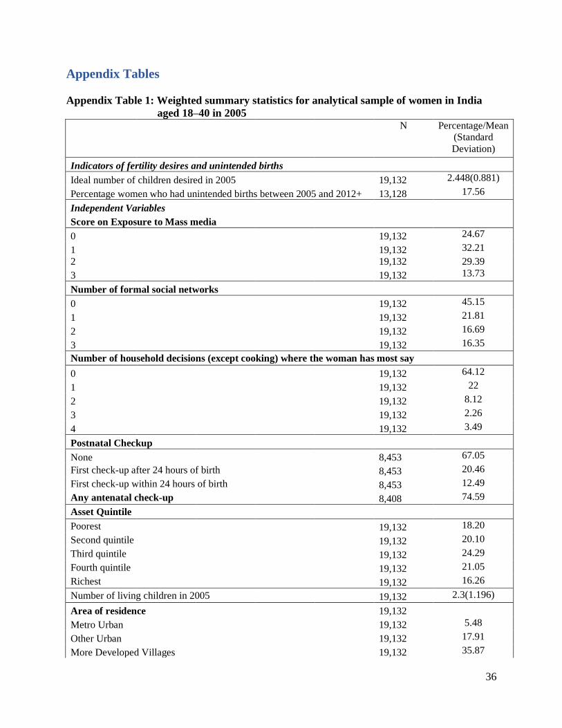
36
Appendix Tables
Appendix Table 1: Weighted summary statistics for analytical sample of women in India
aged 18–40 in 2005 N Percentage/Mean
(Standard
Deviation)
Indicators of fertility desires and unintended births
Ideal number of children desired in 2005 19,132 2.448(0.881)
Percentage women who had unintended births between 2005 and 2012+ 13,128 17.56
Independent Variables
Score on Exposure to Mass media
0 19,132 24.67
1 19,132 32.21
2 19,132 29.39
3 19,132 13.73
Number of formal social networks
0 19,132 45.15
1 19,132 21.81
2 19,132 16.69
3 19,132 16.35
Number of household decisions (except cooking) where the woman has most say
0 19,132 64.12
1 19,132 22
2 19,132 8.12
3 19,132 2.26
4 19,132 3.49
Postnatal Checkup
None 8,453 67.05
First check-up after 24 hours of birth 8,453 20.46
First check-up within 24 hours of birth 8,453 12.49
Any antenatal check-up 8,408 74.59
Asset Quintile
Poorest 19,132 18.20
Second quintile 19,132 20.10
Third quintile 19,132 24.29
Fourth quintile 19,132 21.05
Richest 19,132 16.26
Number of living children in 2005 19,132 2.3(1.196)
Area of residence 19,132
Metro Urban 19,132 5.48
Other Urban 19,132 17.91
More Developed Villages 19,132 35.87

37
N Percentage/Mean
(Standard
Deviation)
Less Developed Villages 19,132 40.73
Religion
Hindu 19,132 83.73
Muslim 19,132 11.23
Other Religion 19,132 5.04
Caste Group
Forward Castes (FC) 19,132 26.80
Scheduled Castes (SC) 19,132 23.10
Scheduled Tribes (ST) 19,132 7.17
Other Backward Classes (OBC) 19,132 42.93
Age Category
18-20 19,132 8.31
21-25 19,132 21.87
26-30 19,132 16.16
31-36 19,132 31.03
36-40 19,132 22.63
Education
Illiterate 19,132 47.85
Incomplete primary 19,132 7.73
Primary 19,132 28.67
Secondary 19,132 8.54
Higher secondary 19,132 4.04
College and higher 19,132 3.17
+ Limited to those who had children less than or equal to ideal family size in 2005.