
Regional Evolutions - Scholars at Harvard · OLIVIER JEAN BLANCHARD Massachusetts Institute of...
75
OLIVIER JEAN BLANCHARD Massachusetts Institute of Technology LAWRENCE F. KATZ Harvard University Regional Evolutions IN 1987, the unemployment ratein Massachusetts averaged 3.2 percent, threepercentage pointsbelow the national rate. Onlyfouryears later, in 1991, it stood at 9.0 percent, more than two points above the national rate. For firms taking investment decisions andfor unemployed workers thinkingabout relocating, the obvious question is whether and when things will return to normal in Massachusetts.This is the issue that we take up in our paper. However, insteadof lookingonly at Massachusetts,we examine the general featuresof regional booms and slumps,studying the behavior of U.S. states over the last 40 years . We attempt to answerfour questions. Whena typical U.S. state over the postwarperiodhas been affectedby an adverse shock to employment,how has it adjusted? Did wages de- cline relative to the rest of the nation? Wereotherjobscreated to replace those jobs destroyed by the shock? Or did workers move out of the state? Ourinterestin these questions extends beyond regional economics. Blocs of countries, notably those in the EuropeanCommunity, are in- creasingly eliminating barriers to the mobilityof goods and factors and movingtoward adopting a common currency. Once these institutional changesare in place, economic interactions amongthese countrieswill moreclosely resemblethose of U.S. states. This paperoffers at least a We thank Rachel Friedberg, Jae Woo Lee, and especially Bill Miracky for research assistance. We thank Timothy Bartik, Hugh Courtney, Steve Davis, Jim Poterba, Xavier Sala-i-Martin, Bill Wheaton, and DRI for data. We thank Timothy Bartik, Rudiger Dorn- busch, Barry Eichengreen, Carol Heim, Ariel Pakes, Danny Quah, Sherwin Rosen, An- drei Shleifer, and participants in many seminars for comments and suggestions. We thank the National Science Foundation for financial support. I
Transcript of Regional Evolutions - Scholars at Harvard · OLIVIER JEAN BLANCHARD Massachusetts Institute of...
OLIVIER JEAN BLANCHARD Massachusetts Institute of Technology
LAWRENCE F. KATZ Harvard University
Regional Evolutions
IN 1987, the unemployment rate in Massachusetts averaged 3.2 percent, three percentage points below the national rate. Only four years later, in 1991, it stood at 9.0 percent, more than two points above the national rate. For firms taking investment decisions and for unemployed workers thinking about relocating, the obvious question is whether and when things will return to normal in Massachusetts. This is the issue that we take up in our paper.
However, instead of looking only at Massachusetts, we examine the general features of regional booms and slumps, studying the behavior of U.S. states over the last 40 years . We attempt to answer four questions. When a typical U.S. state over the postwar period has been affected by an adverse shock to employment, how has it adjusted? Did wages de- cline relative to the rest of the nation? Were otherjobs created to replace those jobs destroyed by the shock? Or did workers move out of the state?
Our interest in these questions extends beyond regional economics. Blocs of countries, notably those in the European Community, are in- creasingly eliminating barriers to the mobility of goods and factors and moving toward adopting a common currency. Once these institutional changes are in place, economic interactions among these countries will more closely resemble those of U.S. states. This paper offers at least a
We thank Rachel Friedberg, Jae Woo Lee, and especially Bill Miracky for research assistance. We thank Timothy Bartik, Hugh Courtney, Steve Davis, Jim Poterba, Xavier Sala-i-Martin, Bill Wheaton, and DRI for data. We thank Timothy Bartik, Rudiger Dorn- busch, Barry Eichengreen, Carol Heim, Ariel Pakes, Danny Quah, Sherwin Rosen, An- drei Shleifer, and participants in many seminars for comments and suggestions. We thank the National Science Foundation for financial support.
I
2 Br-ookings Papers on Economic Activity, 1:1992
glimpse of the nature and the strength of the macroeconomic adjustment mechanisms upon which these countries increasingly will rely.
We start by drawing a general picture of state evolutions over the last 40 years. The most striking feature is the range of employment growth rates across states. Over the last 40 years, some states have consistently grown at 2 percent above the national average, while some states have barely grown, with rates 2 percent below the national average. Rather than leading to fluctuations around trends, employment shocks typically have permanent effects. A state that experiences an acceleration or a slowdown in growth can expect to return to the same growth rate, but on a permanently different path of employment. The picture is very dif- ferent when one looks at unemployment rates. Relative unemployment rates have exhibited no trend; moreover, shocks to relative unemploy- ment rates have lasted for only one-half decade or so. Thus unemploy- ment patterns present an image of vacillating state fortunes as states move from above to below the national unemployment rate, and vice versa. Finally, the last 40 years have been characterized by a steady con- vergence of relative wages, a fact documented recently by Robert Barro and Xavier Sala-i-Martin (using personal income per capita rather than wages).1 As for unemployment, the effects of shocks to relative wages appear to be transitory, disappearing within a decade or so.
We next develop a simple model that can account for these facts. We think of states as producing different bundles of goods, all sold on the national market. We assume that production takes place under constant returns and that there is infinite long-run mobility of both workers and firms. Under these two assumptions, our model implies that differences in the amenities offered by states to either workers or firms lead to per- manent differences in growth rates. However, while employment growth rates differ, labor and product mobility lead to a stable structure of unemployment and wage differentials. Thus the model can explain the observed trends. Moreover, the model can help us think about the shocks and mechanisms underlying regional slumps and booms. As states produce different bundles of goods, they experience different shocks to labor demand and thus experience state-specific fluctuations. Shocks to labor demand first lead to movements in relative wages and unemployment. These in turn trigger adjustments through both labor
1. Barro and Sala-i-Martin (1991).
Olivier Jean Blanchard and Lawrence F. Katz 3
and firm mobility, until unemployment and wages have returned to nor- mal. By then, however, employment is permanently affected; to what extent depends on the relative speed at which workers and firms adjust to changes in wages and unemployment. In the rest of the paper, we use this model as a guide to interpreting the joint movements in relative em- ployment, unemployment, wages, and prices.2
Our third section clears some empirical underbrush. First, we exam- ine the issue of how much of the movement in state employment is com- mon to states and how much is state-specific. The answer is simple. Ag- gregate fluctuations account for most of the year-to-year movement in state employment, but their importance declines steadily over longer horizons. We then address the practical issue of how one should define and construct state relative variables. After considering alternatives, we define all variables as logarithmic deviations from the national average.
We then look at joint movements in employment, unemployment, and participation. We find very similar results across states. A negative shock to employment leads initially to an increase in unemployment and a small decline in participation. Over time, the effect on employment in- creases, but the effect on unemployment and participation disappears after approximately five to seven years. Put another way, a state typi- cally returns to normal after an adverse shock not because employment picks up, but because workers leave the state. These results raise an ob- vious set of questions: does employment fail to pick up because wages have not declined enough or because lower wages are not enough to boost employment?
We take up that question in the next section, where we examine joint fluctuations in employment, unemployment, wages, and prices. We find that in response to an adverse shock in employment, nominal wages de- cline strongly before returning to normal after approximately 10 years. This decline triggers some recovery in employment, but the response of job creation to wage declines is not sufficient to fully offset the initial shock. Using prices as well as wages, we characterize the response of consumption wages to employment shocks. We find that consumption wages decline little in response to such shocks because housing prices, in particular, respond strongly to employment shocks. Thus migration
2. To our knowledge, such a description is not available in the regional literature. An important exception is Bartik (1991), which covers some of the same ground as we do and provides a careful literature survey. We relate our conclusions to Bartik's below.
4 Brookings Paper-s on Economic Activity, 1:1992
in response to shocks appears to result more from changes in unemploy- ment than from changes in relative consumption wages.
Throughout our paper, we identify innovations in employment with shocks to labor demand. Because we consistently find that positive shocks to employment increase wages and reduce unemployment, we are comfortable with this identification assumption. At the end of the pa- per, we follow an alternative and more conventional approach. We ex- amine the effects of two observable and plausibly exogenous demand shocks: defense contracts, and predicted growth rates of employment, using the state industry shares and the national growth rates for each in- dustry. We characterize their effects on employment and unemploy- ment. The picture that emerges is consistent with our earlier findings: the effects on unemployment of employment changes predicted by changes in defense spending and by our industry mix instrument are quite similar to those we estimated for overall innovations in em- ployment.
In the conclusion, we summarize the mechanisms underlying typical regional slumps and booms. Having done so, we return to the case of Massachusetts. We then take up three larger issues. First, we ask whether the adjustment process that we have characterized is efficient. In response to shocks, should workers or jobs move? Our empirical work, which is largely descriptive, cannot answer the question, but the results provide a few hints. We indicate how sharper conclusions could result from further micro-empirical work on the nature of the labor mi- gration and on the ways in which shocks affect the process of job cre- ation and destruction. We then draw the implications of our findings for an understanding of differences in regional growth, because we think- and our model formalizes-that the dynamic mechanisms at work are largely the same. Finally, we discuss the implications and limits of our analysis for European countries as they move to form a common cur- rency area.
Background
We begin by laying out basic facts about regional evolutions of em- ployment, unemployment, and wages in the postwar period.
Olivier Jean Blanchard and Lawrence F. Katz 5
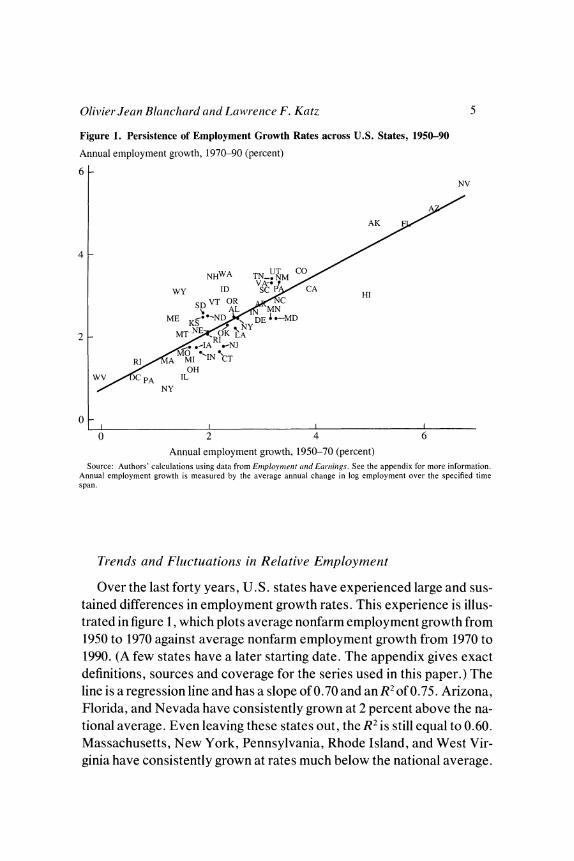
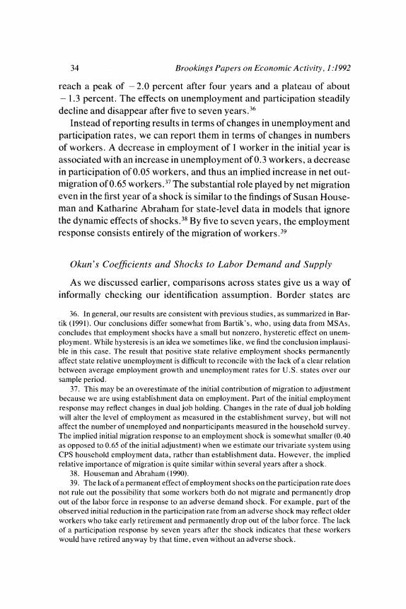
Figure 1. Persistence of Employment Growth Rates across U.S. States, 1950-90
Annual employment growth, 1970-90 (percent)
6 NV
AK
4
NHWA TN2UM CO
WY ID S AHI
SM D VT DE MD
0~~~~~~~~0 A
2 MT AI I]
RI M?I '~O',IN "'CT OH
WV IL
/ ~~NY
0 2 4 6 Annual employment growth, 1950-70 (percent)
Source: Authors' calculations using data from Employment anid Earninlgs. See the appendix for more information. Annual employment growth is measured by the average annual change in log employment over the specified time span.
Trends and Fluctuations in Relative Employment
Over the last forty years, U.S. states have experienced large and sus- tained differences in employment growth rates. This experience is illus- trated in figure 1, which plots average nonfarm employment growth from 1950 to 1970 against average nonfarm employment growth from 1970 to 1990. (A few states have a later starting date. The appendix gives exact definitions, sources and coverage for the series used in this paper.) The line is a regression line and has a slope of 0.70 and an R2 of 0.75. Arizona, Florida, and Nevada have consistently grown at 2 percent above the na- tional average. Even leaving these states out, the R2 is still equal to 0.60. Massachusetts, New York, Pennsylvania, Rhode Island, and West Vir- ginia have consistently grown at rates much below the national average.
6 Brookings Papers on Economic Activity, 1:1992
The variation in growth rates is substantially greater among large U.S. states than among European countries.3
It is true that, over much longer periods, trends in state relative em- ployment growth have changed. The Northeast grew before relatively declining, the South stagnated before growing, and so on. However, over the postwar period, those trends have been surprisingly stable.4 Thus figure 1 puts such stories as the turnaround of the South after the introduction of civil rights in the 1960s and the "Massachusetts miracle" of the early 1980s in the proper perspective.
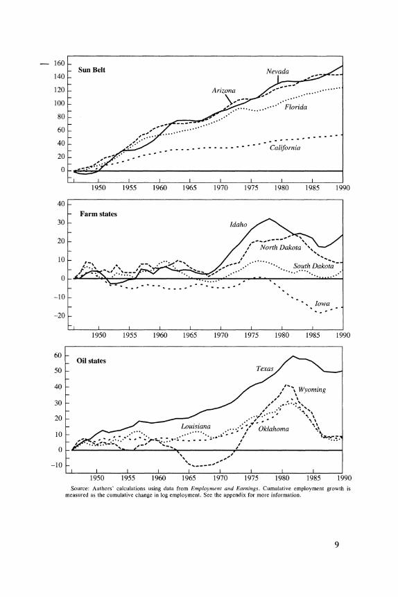
Figure 2 gives a sense of regional trends as well as fluctuations by showing the evolution of employment for a number of states. It plots em- ployment for New England, the Mid-Atlantic states, the Rust Belt, the Sun Belt, the farm states, and the oil states since 1947, measured relative to U.S. aggregate employment. The Massachusetts miracle of the 1980s is little more than a blip on a downward trend. The experience of New York is similarly depressing. Ohio and Illinois also display steady rela- tive employment losses, with losses accelerating in the late 1970s. Mich- igan's substantial postwar relative employment decline is concentrated in two sharp adverse shocks that affected the auto industry in 1956-58 and 1979-82. In contrast to those states, the Sun Belt states have grown consistently since 1947; note the size of the scale of the vertical axis. Two sets of states-not surprisingly, the farm and the oil states-exhibit a different behavior. The farm states do not exhibit a trend, but rather large fluctuations, culminating in the farm crisis of the 1980s.5 The oil states exhibit a boom in the 1970s, followed by a bust in the 1980s.
Having displayed our findings graphically, we turn to a formal charac- terization of the stochastic behavior of relative employment move- ments. We define nit as the logarithm of employment in state i in year t minus the logarithm of U.S. employment in year t. Because most states clearly have a trend in relative employment, and we do not find the hy- pothesis of deterministic trends appealing, our assumption is that their process contains a unit root. We nevertheless test for evidence against a unit root by running for each state
3. See, for example, Krugman (1992). 4. In fact, an influential article by Borts (1960) documents that state employment
growth trends were fairly persistent from 1909 to 1953. 5. However, in looking at farm states, remember that our data measure nonfarm em-
ployment.
Olivier Jean Blanchar-d atnd Lawrence F. Katz 7
(1) Anit = Oli + -2i (L) Ani,tl I+ ? a3i ni,t- I+ ?t4i T + rit,
where T is time and nit is a disturbance term. We allow for four lags in O2i (L).6 The period of estimation is 1952-90.
The evidence from augmented Dickey-Fuller tests, which look at the t statistic on (3i, the coefficient associated with the lagged level, is mixed. In all states, the coefficient on the lagged level is negative. But in only three states-Massachusetts, South Dakota, and Wyoming-is it sig- nificant at the 5 percent level. Thus, given our prior, we impose from here on the hypothesis of a unit root in relative employment.7
We then estimate the univariate process for employment by running from 1952 to 1990: (2) A\nit =Oli + t2i (L) A\ni, l- + q it
We allow for four lags in O2i (L). From these estimated coefficients, we derive the associated impulse response, which gives the response of the level of relative employment to an innovation in -q implied by equation 2. Regression coefficients and impulse responses are given in table 1.
The results in table 1 are obtained by pooling all states together, allowing for state effects. Throughout the paper, we take advantage of the cross section and time series dimensions of our data by estimating equations not only state-by-state but also for pooled sets of states. When pooling, we either pool all 50 states and the District of Columbia together as in table 1, or pool them by Census division.8 There are nine such divi- sions; they are relatively homogeneous and thus provide a natural way to pool states.9 Because of their different patterns, we also often look separately at farm states and oil and mineral states. We define farm states as those states in which earnings from agriculture accounted for
6. We include a time trend to allow the process to have a deterministic trend under the alternative hypothesis. For further discussion, see, for example, Campbell and Perron (1991).
7. We have checked the robustness of our results below to relaxing this assumption. The impulse responses obtained from estimating a univariate process assuming stationar- ity of relative employment around a deterministic trend are very similar to those reported in table 1, at least for the first 15 years or so.
8. For the sake of brevity, in the rest of this paper, we refer to the 50 U.S. states and the District of Columbia as the 51 states.
9. The Census uses two classification levels, regions and divisions. The four regions- the Northeast, the Midwest, the South, and the West-are very heterogenous and are not an appealing way of grouping states.
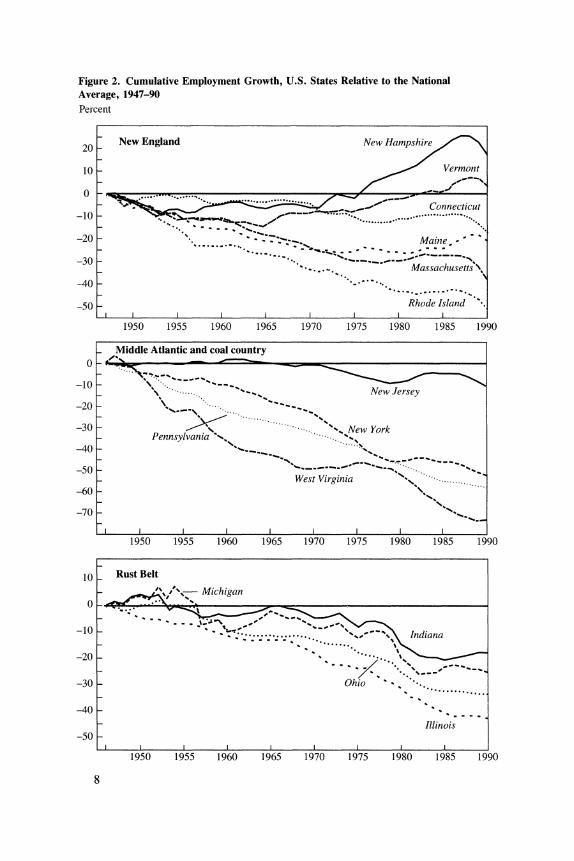
Figure 2. Cumulative Employment Growth, U.S. States Relative to the National Average, 1947-90 Percent
20 - New England New Hampshir
10 Vermont 10
-10 ... .......... -20 .........-...~~~~~~~~~~~~~~.........
-20 - M ai-.e. - a Massachusetts\
-40 -
-50 Rhode Island
1950 1955 1960 1965 1970 1975 1980 1985 1990
_Middle Atlantic and coal country 0-
-10 - \\' 's
-20
-30 New York 40 k ~Pennsylvania >
-40-
-50- _ West Virginia
-60 -
-70
1950 1955 1960 1965 1970 1975 1980 1985 1990
10 Rust Belt
-10 O L i- .: l~% % ndiana
-20
-30 Ohio *..
-40
Illinois -50
1950 1955 1960 1965 1970 1975 1980 1985 1990
8
_ 160 - - Sun Belt Nevada
140_ .
120Arzn
100 ?? 0 ,>. ./ ~~~~~~ ~ ~~~~~Floridal
80
60 -
40 - - - --- -- - -- - California
20-
1950 1955 1960 1965 1970 1975 1980 1985 1990
40 - Farm states
30 - Idaho
20 t / Nor-th Dakota
10 F , " , South Dakota
-10 Iowa
-20
- I I I I I, I _
1950 1955 1960 1965 1970 1975 1980 1985 1990
60 Oil states
50 Texas
40 t,,yoming
30
20 Louisiana Oklhom
10 15 Oklahom
-10 -
F l I I I ~~~~~~~~~~~~~~~~~~~~II I
1950 1955 1960 1965 1970 1975 1980 1985 1990 Source: Authors' calculations using data from Employment atnd Earninlgs. Cumulative employment growth is
measured as the cumulative change in log employment. See the appendix for more information.
10 Br-ookings Papers on Economic Activity, 1:1992
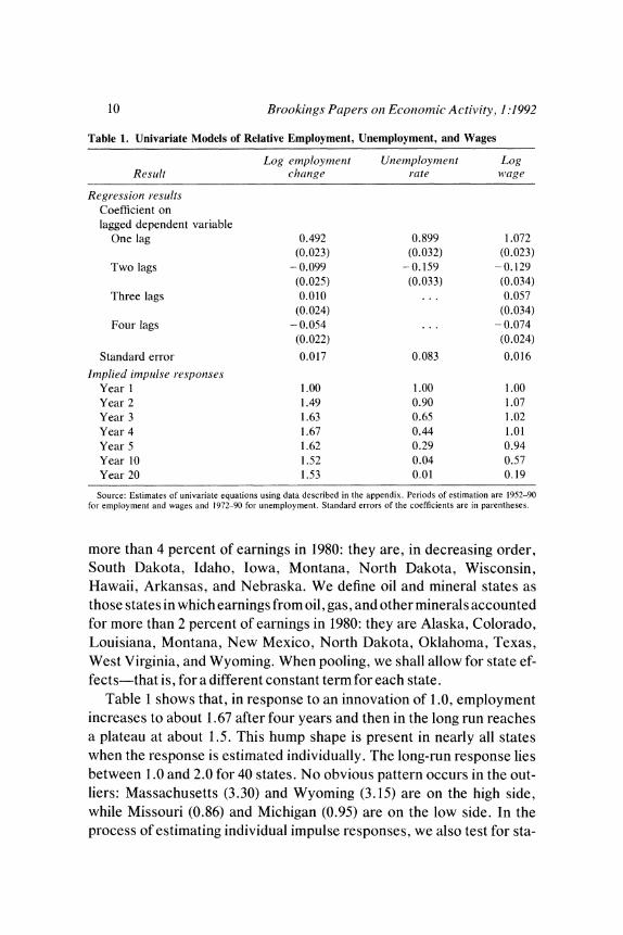
Table 1. Univariate Models of Relative Employment, Unemployment, and Wages
Log employment Uneemploymenit Log Result change rate w,age
Regression results Coefficient on lagged dependent variable
One lag 0.492 0.899 1.072 (0.023) (0.032) (0.023)
Two lags -0.099 -0.159 -0.129 (0.025) (0.033) (0.034)
Three lags 0.010 .. . 0.057 (0.024) (0.034)
Four lags - 0.054 .. . -0.074 (0.022) (0.024)
Standard error 0.017 0.083 0.016
Implied impulse responises Year 1 1.00 1.00 1.00 Year 2 1.49 0.90 1.07 Year 3 1.63 0.65 1.02 Year 4 1.67 0.44 1.01 Year 5 1.62 0.29 0.94 Year 10 1.52 0.04 0.57 Year 20 1.53 0.01 0.19
Source: Estimates of univariate equations using data described in the appendix. Periods of estimation are 1952-90 for employment and wages and 1972-90 for unemployment. Standard errors of the coefficients are in parentheses.
more than 4 percent of earnings in 1980: they are, in decreasing order, South Dakota, Idaho, Iowa, Montana, North Dakota, Wisconsin, Hawaii, Arkansas, and Nebraska. We define oil and mineral states as those states in which earnings from oil, gas, and other minerals accounted for more than 2 percent of earnings in 1980: they are Alaska, Colorado, Louisiana, Montana, New Mexico, North Dakota, Oklahoma, Texas, West Virginia, and Wyoming. When pooling, we shall allow for state ef- fects-that is, for a different constant term for each state.
Table 1 shows that, in response to an innovation of 1.0, employment increases to about 1.67 after four years and then in the long run reaches a plateau at about 1.5. This hump shape is present in nearly all states when the response is estimated individually. The long-run response lies between 1.0 and 2.0 for 40 states. No obvious pattern occurs in the out- liers: Massachusetts (3.30) and Wyoming (3.15) are on the high side, while Missouri (0.86) and Michigan (0.95) are on the low side. In the process of estimating individual impulse responses, we also test for sta-
Olivier Jean Blanchard and Lawrence F. Katz 11
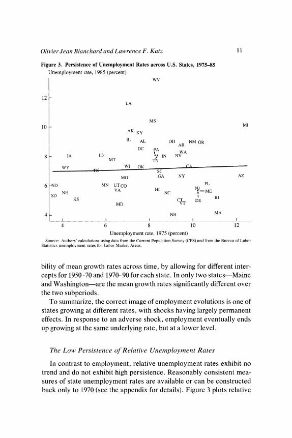
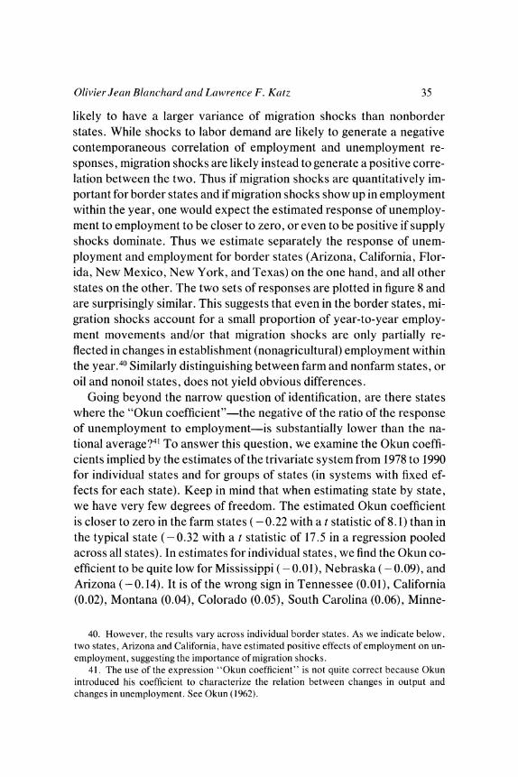
Figure 3. Persistence of Unemployment Rates across U.S. States, 1975-85 Unemployment rate, 1985 (percent)
WV
12 - LA
MS
10 _ Ml AK KY
IL AL OH NMOR AR
DC PA WA
8 - IA ID *IN NV MT TN
WY WI OK CA
MO GA NY AZ
6 AD MN UT CO FL VA HI NJ M
SD NE NC I*-ME KS CT DE RI
MD VT
4 NH MA I IIII
4 6 8 10 12
Unemployment rate, 1975 (percent) Source: Authors' calculations using data from the Current Population Survey (CPS) and from the Bureau of Labor
Statistics unemployment rates for Labor Market Areas.
bility of mean growth rates across time, by allowing for different inter- cepts for 1950-70 and 1970-90 for each state. In only two states-Maine and Washington-are the mean growth rates significantly different over the two subperiods.
To summarize, the correct image of employment evolutions is one of states growing at different rates, with shocks having largely permanent effects. In response to an adverse shock, employment eventually ends up growing at the same underlying rate, but at a lower level.
The Low Persistence of Relative Unemployment Rates
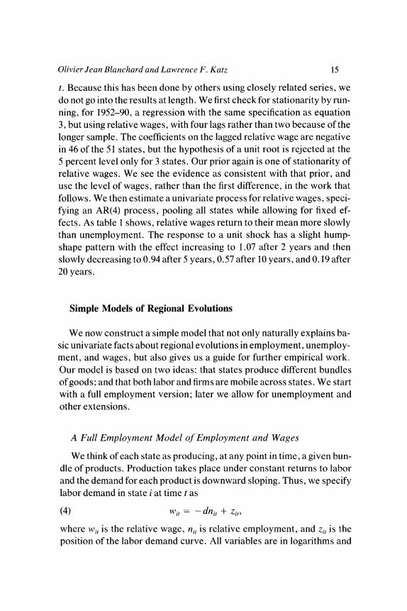
In contrast to employment, relative unemployment rates exhibit no trend and do not exhibit high persistence. Reasonably consistent mea- sures of state unemployment rates are available or can be constructed back only to 1970 (see the appendix for details). Figure 3 plots relative
12 Brookings Paper-s oni Economic Activity, 1 :1992
unemployment rates 10 years apart, in 1975 and in 1985. The line is a regression line with a slope of 0.03, a t statistic of 0.2, and an R2 of 0.00. The fact that relative unemployment rates show low persistence was al- ready mentioned by Stephen Marston and Lawrence Summers.'0 It is probably this fact that underlies the frequently stated account of fluctu- ating state fortunes; however, as we have seen, a different picture is given by employment evolutions.
We must admit that the two dates used in figure 3 yield a unusually low correlation. Had we used, say, relative unemployment rates in 1970 and 1990, the regression coefficient would be 0.41, with a t statistic of 3.8 and an R2 of 0.23.11 This positive correlation has two potential origins. The first is that relative unemployment rates have different means across states. The second is that deviations from means are very persistent. It turns out that the positive correlation comes mostly from the means, not from the persistence of the effect of shocks. As a simple exercise, for example, one can exclude the farm states from the regres- sion, because they clearly have lower average unemployment rates. The coefficient then drops to 0.24, with an R2 of 0.11.
To go further, we more formally examine the stochastic behavior of relative unemployment rates. We define uit as the unemployment rate in state i at time t minus the U.S. unemployment rate. We first check for stationarity by running, for the period 1972-90,
(3) Auit = oxli + o1x2i (L) uiu,t-1 + X3L ui,t1 I + qit-
Because relative unemployment rates do not exhibit a trend, we do not allow for one in the regression. Because the sample period is shorter than for employment, we allow for only two lags in cv2i (L). The results from augmented Dickey-Fuller tests are again mixed. In all states, coef- ficients on the lagged level are negative, usually between -0.2 and
10. Marston (1985); Summers (1986). 11. Neumann and Topel (1991) report substantially higher intertemporal correlations
of relative state unemployment rates for the 1970-85 period using labor-force-weighted correlations of three-year moving averages of relative state insured unemployment rates. The differences between their results and ours do not reflect their use of labor force weights or smoothed unemployment rates (three year averages); rather, they reflect the differences between insured and overall unemployment rates. Differences in the generos- ity and administration of state unemployment insurance systems lead to persistent mean differences in insured unemployment rates across states that lead to much higher intertem- poral correlations of insured, than of overall, state unemployment rates.
Olivier Jean Blanchard and Lawrence F. Katz 13
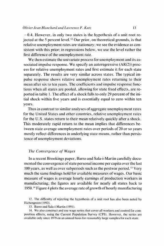
- 0.4. However, in only two states is the hypothesis of a unit root re- jected at the 5 percent level. 12 Our prior, on theoretical grounds, is that relative unemployment rates are stationary; we see the evidence as con- sistent with this prior; in regressions below, we use the level rather the first difference of the unemployment rate.
We then estimate the univariate process for unemployment and its as- sociated impulse response. We specify an autoregressive (AR(2)) proc- ess for relative unemployment rates and first estimate it for each state separately. The results are very similar across states. The typical im- pulse response shows relative unemployment rates returning to their mean after six to ten years. The coefficients and impulse response func- tions when all states are pooled, allowing for state fixed effects, are re- ported in table 1. The effect of a shock falls to only 29 percent of the ini- tial shock within five years and is essentially equal to zero within ten years.
Thus in contrast to similar analyses of aggregate unemployment rates for the United States and other countries, relative unemployment rates for the U.S. states return to their mean relatively quickly after a shock. This moderately rapid return to the mean implies that differences be- tween state average unemployment rates over periods of 20 or so years mostly reflect differences in underlying state means, rather than persis- tence of unemployment deviations.
The Convergence of Wages
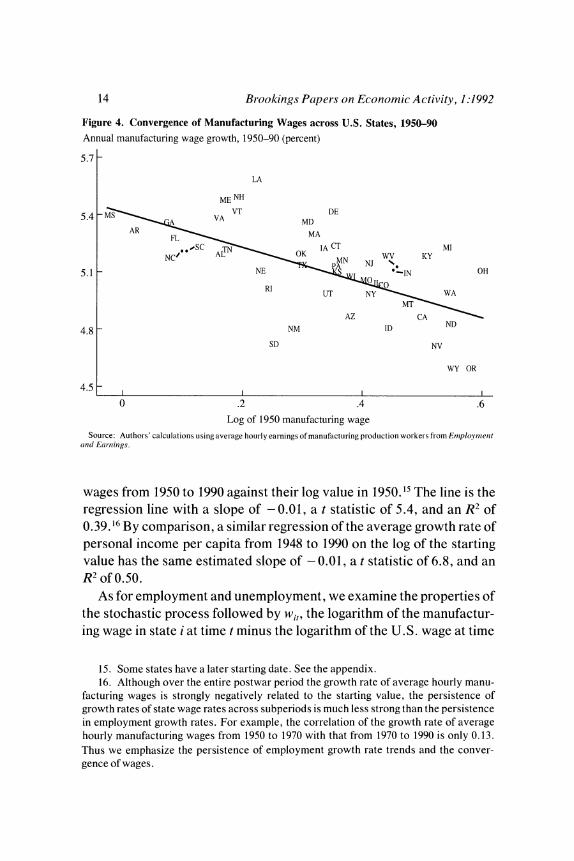
In a recent Brookings paper, Barro and Sala-i-Martin carefully docu- mented the convergence of state personal income per capita over the last 100 years, as well as over subperiods such as the postwar period. 13 Very much the same findings hold for available measures of wages. Our basic measure of wages is average hourly earnings of production workers in manufacturing; the figures are available for nearly all states back to 1950.14 Figure 4 plots the average rate of growth of hourly manufacturing
12. The difficulty of rejecting the hypothesis of a unit root has also been noted by Eichengreen (1992).
13. Barro and Sala-i-Martin (1991). 14. We also construct and use wage series that cover all workers and control for com-
position effects, using the Current Population Survey (CPS). However, the series are available only since 1979 on an annual basis for reasonably large samples for each state.
14 Br-ookings Paper-s on Economic Activity, 1:1992
Figure 4. Convergence of Manufacturing Wages across U.S. States, 1950-90 Annual manufacturing wage growth, 1950-90 (percent)
5.7 -
LA
ME NH
5.48- VA VT DE
SD DN
FL MA
F
z S~C .A5--E WV KY
RI UT NY WA
AZ CA
4.8 ~~ ~ ~ ~ ~~~NM ID ND
SD NV
WY OR
4.5
0 .2 .4 .6
Log of 1950 manufacturing wage Source: Authors' calculations using average hourly earnings of manufacturing production workers from Em7ploymi71ent
antid Eanssinzgs.
wages from 1950 to 1990 against their log value in 1950.15 The line is the regression line with a slope of - 0.01, a t statistic of 5.4, and an R2 of 0.39. 16 By comparison, a similar regression of the average growth rate of personal income per capita from 1948 to 1990 on the log of the starting value has the same estimated slope of - 0.01, a t statistic of 6.8, and an R2 of 0.50.
As for employment and unemployment, we examine the properties of the stochastic process followed by w,t, the logarithm of the manufactur- ing wage in state i at time t minus the logarithm of the U.S. wage at time
15. Some states have a later starting date. See the appendix. 16. Although over the entire postwar period the growth rate of average hourly manu-
facturing wages is strongly negatively related to the starting value, the persistence of growth rates of state wage rates across subperiods is much less strong than the persistence in employment growth rates. For example, the correlation of the growth rate of average hourly manufacturing wages from 1950 to 1970 with that from 1970 to 1990 is only 0.13. Thus we emphasize the persistence of employment growth rate trends and the conver- gence of wages.
Olivier Jean Blanchard and Lawrence F. Katz 15
t. Because this has been done by others using closely related series, we do not go into the results at length. We first check for stationarity by run- ning, for 1952-90, a regression with the same specification as equation 3, but using relative wages, with four lags rather than two because of the longer sample. The coefficients on the lagged relative wage are negative in 46 of the 51 states, but the hypothesis of a unit root is rejected at the 5 percent level only for 3 states. Our prior again is one of stationarity of relative wages. We see the evidence as consistent with that prior, and use the level of wages, rather than the first difference, in the work that follows. We then estimate a univariate process for relative wages, speci- fying an AR(4) process, pooling all states while allowing for fixed ef- fects. As table 1 shows, relative wages return to their mean more slowly than unemployment. The response to a unit shock has a slight hump- shape pattern with the effect increasing to 1.07 after 2 years and then slowly decreasing to 0.94 after 5 years, 0.57 after 10 years, and 0.19 after 20 years.
Simple Models of Regional Evolutions
We now construct a simple model that not only naturally explains ba- sic univariate facts about regional evolutions in employment, unemploy- ment, and wages, but also gives us a guide for further empirical work. Our model is based on two ideas: that states produce different bundles of goods; and that both labor and firms are mobile across states. We start with a full employment version; later we allow for unemployment and other extensions.
A Full Employment Model of Employment and Wages
We think of each state as producing, at any point in time, a given bun- dle of products. Production takes place under constant returns to labor and the demand for each product is downward sloping. Thus, we specify labor demand in state i at time t as
(4) wit = - dnit + zit
where wit is the relative wage, nit is relative employment, and zit is the position of the labor demand curve. All variables are in logarithms and
16 Brookings Papers on Economic Activity, 1:1992
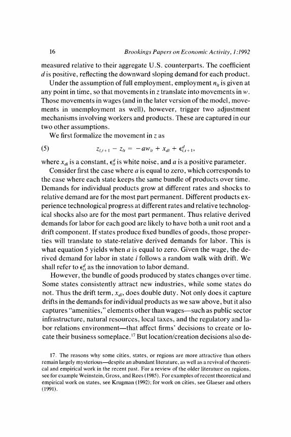
measured relative to their aggregate U.S. counterparts. The coefficient d is positive, reflecting the downward sloping demand for each product.
Under the assumption of full employment, employment nit is given at any point in time, so that movements in z translate into movements in w. Those movements in wages (and in the later version of the model, move- ments in unemployment as well), however, trigger two adjustment mechanisms involving workers and products. These are captured in our two other assumptions.
We first formalize the movement in z as
(5) zi,t+ - - -awit + Xdi + ?-,t+ I
where xdi is a constant, Ed is white noise, and a is a positive parameter. Consider first the case where a is equal to zero, which corresponds to
the case where each state keeps the same bundle of products over time. Demands for individual products grow at different rates and shocks to relative demand are for the most part permanent. Different products ex- perience technological progress at different rates and relative technolog- ical shocks also are for the most part permanent. Thus relative derived demands for labor for each good are likely to have both a unit root and a drift component. If states produce fixed bundles of goods, those proper- ties will translate to state-relative derived demands for labor. This is what equation 5 yields when a is equal to zero. Given the wage, the de- rived demand for labor in state i follows a random walk with drift. We shall refer to d as the innovation to labor demand.
However, the bundle of goods produced by states changes over time. Some states consistently attract new industries, while some states do not. Thus the drift term, Xdi, does double duty. Not only does it capture drifts in the demands for individual products as we saw above, but it also captures "amenities," elements other than wages-such as public sector infrastructure, natural resources, local taxes, and the regulatory and la- bor relations environment-that affect firms' decisions to create or lo- cate their business someplace. 17 But location/creation decisions also de-
17. The reasons why some cities, states, or regions are more attractive than others remain largely mysterious-despite an abundant literature, as well as a revival of theoreti- cal and empirical work in the recent past. For a review of the older literature on regions, see for example Weinstein, Gross, and Rees (1985). For examples of recent theoretical and empirical work on states, see Krugman (1992); for work on cities, see Glaeser and others (1991).
Olivier Jean Blanchard and Lawrence F. Katz 17
pend on wages. This is what is captured by the parameter a: everything else being equal, lower wages make a state more attractive.'8 One im- portant question is whether in response to an adverse shock that de- creases wages, everything else would indeed remain equal. This matter will be easier to discuss when we introduce unemployment to our model below. Note that the above formulation implies a short-run elasticity of a and a long-run elasticity of infinity.
We formalize the movement in the labor force, n, as
(6) nit+1 - nit - bwit + Xsi + Esi1t+,
where xsi is a constant, Es is white noise, and b is a positive parameter. Most of the differences in average employment growth rates across
states are due to migration, rather than to differences in natural popula- tion growth rates. 19 In fact, the correlation of state employment growth and net migration rates is 0.84 for the 1950-87 period and 0.91 for the 1970-87 period.20 Thus we can think of the equation as characterizing migration of workers.
Equation 6 allows migration to depend on three terms: the relative wage, a drift term, and a stochastic component. The drift term, xsi, cap- tures amenities, those nonwage factors that affect migration. Stories about the attractiveness of the California lifestyle and Sun Belt weather are common features of descriptions of regional migration patterns. By assuming that these amenities-and the amenities affecting firms, Xdi, in equation 5-are time-invariant, we ignore such factors as the introduc- tion of air conditioning, which clearly increased the attractiveness of the South. Allowing amenities to evolve would, in our model, lead to changes in the underlying growth rate of a state. But as we showed ear- lier, little evidence exists of changes in underlying state growth rates
18. A straightforward extension would be to make firms' location decisions a function of current and future expected wages. The obvious implication is that firms will respond less to current wages if (as is the case in this model) wages are expected to return to their state-specific mean.
19. See Turek (1985) for an analysis of the roles played by net migration and natural population increase in differences in regional population growth in the twentieth century.
20. The net migration rates refer to averages of rates for the subperiods 1950-60, 1960- 70, 1970-80, and 1980-87, weighted by the lengths of the subperiod. The rate for each subperiod is the annual average rate of net migration divided by state population at the start of the subperiod. The migration data include the entire population, not only the work- ing age population. Further information appears in the appendix.
18 Brookings Papers on Economic Activity, 1:1992
over the postwar period, so that we do not pursue that extension. The term, Ei +i, captures those clearly transitory movements in exogenous migration, such as boat lifts, changes in immigration laws, or deteriora- tions of economic conditions in Mexico, that lead to increased migra- tion. We shall refer to Ei as the innovation in labor supply. The wage term captures the effects of wages on migration: everything else being equal, lower wages decrease in-migration.21 Again, the research on mi- gration has emphasized the fact that, in response to an adverse shock, everything else may not be equal; for example, unemployment is an im- portant determinant of migration. We return to this when we introduce unemployment. Lastly, note that the above formulation implies a short- run elasticity of migration to the wage of b and a long-run elasticity of infinity.
Wages and Employment
Under our assumptions, states indeed exhibit different growth rates. Supply and demand innovations permanently affect employment. Aver- age relative wages differ across states, but relative wages are stationary. To see this, we can solve for wages to get
wijt+I = (1 - db - a)wit + (xdi- dxsi) + (E6't+I - dEi t+ )
so that the average relative wage is given by
wi= (1/(a + db))xdi - (dl(a+db))xsi.
We can also solve for employment to get
\ni,t +I = (1 - db - a) Anit + (bxdi + axsi)
? (bEt+j + ? Et+ -(I -a) Es)
so that trend employment growth is given by
Ani = (bl(a + db))Xdi + (al(a + db)) xsi.
As long as there is either labor or product mobility (a or b > 0), rela- tive wages follow a stationary process around state-specific means, with the innovations to labor demand and to labor supply as forcing terms.
21. A useful extension would be to make worker migration decisions a function of cur- rent and future expected wages, as in Braun (1992) and Topel (1986).
Olivier Jean Blanchar-d and Lawr-ence F. Katz 19
Thus, starting from any distribution of relative wages, the distribution of relative wages will converge to a stationary distribution over time.22
In contrast, relative employment grows or declines at an average rate determined by both drifts. In states attractive to workers, states where xsi is positive, the steady flow of workers leads to a lower wage, which in turn triggers a steady flow of new jobs and sustains growth. In states attractive to firms, states where Xdi is positive, the steady flow of firms leads to a higher wage, which in turn triggers an inflow of workers and sustains growth. In contrast to wages, innovations to both labor demand and labor supply permanently affect the level of employment.
The Effects of an Innovation in Labor Demand
Most of our focus below will be on what happens to states that face a shock, adverse or favorable, to the demand for their goods. More for- mally, we examine the effects of an innovation in labor demand. Con- sider, for example, the effects of an adverse shock to employment. De- note by a hat the deviation of a variable from its base (no shock) path. Then, from the equations above, the effects of an innovation of - 1 in period 0 in Ei on wages and employment at time t are given by
wit= -(1 - a - db)t->O,
nit =-b(1 - (1 - a - db)t)/(a + db) -bl(a + db).
A negative innovation to labor demand initially decreases wages. Over time, wages return to normal as net out-migration of workers and job creation reestablish the initial equilibrium. The speed at which wages return to normal is an increasing function of both short-run elas- ticities, a and b.
The response of employment is the more interesting of the two. Ini- tially, employment remains unchanged as wages absorb the adverse shift in demand (by the assumption of full employment). Over time, however, employment decreases relative to its base path to end asymp- totically lower by an amount equal to - bl(a + db). Thus, the long-run decrease in employment depends on the relative values of the short-run elasticities of firms and workers.
22. This is what Barro and Sala-i-Martin (1991) have called a-convergence.
20 Brookings Papers on Economic Activity, 1:1992
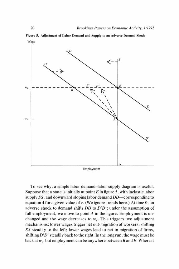
Figure 5. Adjustment of Labor Demand and Supply to an Adverse Demand Shock
Wage
D
wo ~ ~ ~ ~ ~ ~ ' E" E
Wa ~A D'
s
Employment
To see why, a simple labor demand-labor supply diagram is useful. Suppose that a state is initially at point E in figure 5, with inelastic labor supply SS, and downward sloping labor demand DD-corresponding to equation 4 for a given value of z. (We ignore trends here.) At time 0, an adverse shock to demand shifts DD to D'D'; under the assumption of full employment, we move to point A in the figure. Employment is un- changed and the wage decreases to wa. This triggers two adjustment mechanisms: lower wages trigger net out-migration of workers, shifting SS steadily to the left; lower wages lead to net in-migration of firms, shifting D'D' steadily back to the right. In the long run, the wage must be back at wo, but employment can be anywhere between B and E. Where it
Olivier Jean Blanchard and Lawrence F. Katz 21
ends up depends on the speed at which the two loci shift, on the relative speeds at which workers leave and firms come. If workers leave faster than firms come, the outcome is E'. If workers move more slowly, the outcome is E".
The importance of the relative speeds in the adjustment process is best illustrated by an example, which also shows the many aspects of reality hidden in a and b. The computer manufacturer Wang is located in Lowell, Massachusetts. Because the relative demand for minicom- puters fell sharply, the unemployment rate in Lowell has sharply in- creased, to an average of 9.7 percent in 1991. Lowell is thus a potentially attractive place for firms, say, in the microcomputer industry, to relo- cate: if they come, they could hire from a pool of qualified workers at lower wages than firms could have a few years ago. Will those firms come and come in time? Will workers, many of them unemployed, and many probably liquidity-constrained, be able to wait for firms to come? Or will workers have to move before new jobs have been created, thus negating the reasons for firms to come in the first place? Such different outcomes are captured by points such as E' and E" in figure 5.
We have concentrated on innovations in labor demand. A symmetri- cal analysis applies to innovations in labor supply. A positive innovation to labor supply decreases wages. Over time, wages return to normal. And in the process, employment increases relative to its base path to end up asymptotically higher by al(a + db). Again, the long-run effect de- pends on the ratio of the two elasticities. If, for example, a is equal to zero, the initial increase in labor supply is fully offset by out-migration in the long run.
Allowing for Unemnployment
We now relax the assumption that wages adjust so as to maintain full employment. Under any realistic description of wage determination, the adjustment process is likely to involve movements in unemployment, as well as in wages. To capture that, we modify the model as follows:
Wit = - d(n,* - Uit) + zit;
cwit Uit;
n*+I- n* bwit - guit + X,i
+ E5t+l;
7 - zit ?a
Xwit ? E/+1-
22 Brookings Papers on Econiomic Activity, 1:1992
The variable n* stands for the logarithm of the labor force in state i at time t, and uit is the unemployment rate in state i at time t, defined as the ratio of unemployment to employment, so that the logarithm of employ- ment is approximately given by n* - uit.23
Our specification of labor demand in the first equation is the same as before, but is now expressed as a relation between unemployment and the wage, given the labor force. The second equation is new: it states, in the simplest possible way, that higher unemployment leads to lower wages. A more sophisticated specification would allow for the fact that wages are likely to depend on vacancies as well, and thus on the trend in z; we shall not explore this specification. The semi-elasticity of wages with respect to the unemployment rate is given by (1/c).
The important modifications are in the specification of the last two equations. Research on labor migration emphasizes the importance of unemployment and job availability in determining migration.24 Thus the third equation allows labor mobility to depend not only on relative wages, but also on relative unemployment. How does unemployment- given wages-affect job creation and the decisions of firms to migrate? As the example of Lowell suggests, higher unemployment implies a larger pool of workers to choose from and thus makes firms more likely to come. But higher unemployment also implies potentially higher tax rates, lower quality public services, or fiscal crises and their attending uncertainty. These factors are likely to deter firms from coming to de- pressed states. As a first approximation, we assume in the last equation that firms' decisions do not depend on unemployment-although we would be as willing to assume that firms are reluctant to locate in areas with high unemployment. The algebra is straightforward and the conclu- sions can be stated in words.
An underlying positive drift in relative labor demand, xdi, leads to a positive relative trend in employment, higher-than-average wages, and lower-than-average unemployment.25 An underlying positive drift in rel-
23. To see that, let U, E, and L denote the levels of unemployment, employment, and the labor force. Note that it = UIE ln(l + (UIE)) = ln(L)-ln(E). Thus (n1* - it) ln(L) - ln(L) + ln(E) = ln(E).
24. See, for example, DaVanzo (1978) and Greenwood (1985). 25. This is one place where a more elaborate specification of wage determination could
lead to different correlations. High employment growth may lead to more vacancies and higher wait unemployment.
Olivier Jean Blanchard and Lawrence F. Katz 23
ative labor supply, x,i, leads to a positive relative trend in employment, lower-than-average wages, and higher-than-average unemployment.
An adverse shock in the relative demand for labor initially increases unemployment and decreases wages. Over time, net out-migration of workers and net in-migration of firms lead to a decline in unemployment and an increase in wages. How much of the adjustment occurs through the creation of new jobs and how much occurs through the migration of workers depends again on the short-run elasticities. However, an im- portant difference exists, compared to our earlier, full employment, story. While both high unemployment and low wages lead to labor mi- gration, only lower wages induce firms to come. Thus the more the initial decline in demand is reflected in unemployment, rather than wages, the larger the long-run effect of adverse shocks on employment.
Other Extensions
The model can easily accommodate a number of extensions. One is to allow for capital accumulation by existing firms.26 The effects of capital accumulation by existing firms are very different from those induced by the movement of new firms. While adverse shocks to demand may lead, through lower wages, to the in-migration of firms, they decrease the re- turn to capital in existing firms. This in turn leads to capital decumula- tion and the amplification of the initial shock. This makes it more likely that an adverse shock in demand leads to a larger effect on employment in the long run than in the short run. Another extension we have already mentioned would be to recognize that mobility decisions are likely to be forward looking, so that the speed at which unemployment and wages return to normal will affect the initial mobility decisions.
However, other extensions would more drastically change the nature of the model. Two such extensions are the introduction of land as a scarce factor and the presence of externalities. One of the main implica- tions of our model is thatfixed differences in amenities, either for work- ers or for firms, lead to sustained differences in growth rates. This result comes in turn from the underlying assumptions of constant returns in production and infinite long-run mobility of firms and workers. If we were to introduce scarce land, the model would lose its property of con-
26. See Blanchard (1991).
24 Brookings Paper s on Economic Activity, 1:1992
stant returns. Fixed amenities would no longer lead to permanent differ- ences in growth rates, but instead to differences in employment levels and land prices.27 If we were instead to introduce externalities (a theme explored recently by Paul Krugman and others), for example by making the attractiveness of a state, Xdi, no a longer a constant, but an increasing function of the number of products in the state, the model would gener- ate instead accelerating growth.28 We have no doubt that scarcity of land and various forms of externalities associated with population density are relevant, although perhaps more for cities than for states; we see the constant returns assumptions and its implication of constant growth dif- ferentials as a convenient simplification and a good approximation to the data over the postwar period.
Identification: Labor Demand or Labor Supply Shocks?
In our empirical work, we estimate the reduced forms-vector auto- regressions (VAR)-corresponding to our model in its different incarna- tions and trace the effects of adverse shocks to demand, the Ed, on such factors as employment, unemployment, and wages. This raises the issue of how we identify Ed.
Our basic approach to identification is simple: we associate unfore- castable movements in employment with innovations in labor demand. This assumption is approximately correct if most of the year-to-year un- expected movements in employment are caused by shifts in labor de- mand, rather than by shifts in labor supply (an assumption we find highly plausible). However, we realize that readers may question our identifi- cation restrictions. Thus we pursue two alternative routes.
Our first method is to exploit cross sectional differences in the joint behavior of employment, unemployment, and wages in the data. The relative importance of migration shocks surely varies across states; they are more likely to be important for border states in the South than for states in the Midwest, for example. Thus we examine those border states separately as we go along, looking for systematic differences.29
27. See Roback (1982) for a clear analysis of the joint long-run spatial equilibrium of local land and labor markets in a model with mobile firms and workers.
28. Krugman (1991). 29. A precursor paper, which exploits correlations between employment changes and
wages to identify the role of supply and demand shocks in different urban areas, is Wheaton (1979).
Olivier Jean Blanchard and Lawsrence F. Katz 25
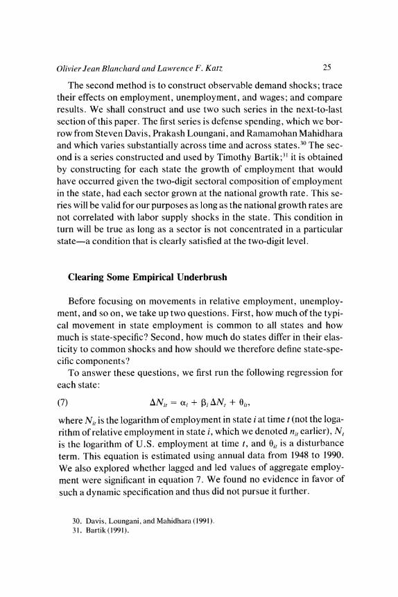
The second method is to construct observable demand shocks; trace their effects on employment, unemployment, and wages; and compare results. We shall construct and use two such series in the next-to-last section of this paper. The first series is defense spending, which we bor- row from Steven Davis, Prakash Loungani, and Ramamohan Mahidhara and which varies substantially across time and across states.30 The sec- ond is a series constructed and used by Timothy Bartik;3' it is obtained by constructing for each state the growth of employment that would have occurred given the two-digit sectoral composition of employment in the state, had each sector grown at the national growth rate. This se- ries will be valid for our purposes as long as the national growth rates are not correlated with labor supply shocks in the state. This condition in turn will be true as long as a sector is not concentrated in a particular state-a condition that is clearly satisfied at the two-digit level.
Clearing Some Empirical Underbrush
Before focusing on movements in relative employment, unemploy- ment, and so on, we take up two questions. First, how much of the typi- cal movement in state employment is common to all states and how much is state-specific? Second, how much do states differ in their elas- ticity to common shocks and how should we therefore define state-spe- cific components?
To answer these questions, we first run the following regression for each state:
(7) ANi, = (i + ?i AN, + ?i,
where Nit is the logarithm of employment in state i at time t (not the loga- rithm of relative employment in state i, which we denoted ni, earlier), N, is the logarithm of U.S. employment at time t, and Oi, is a disturbance term. This equation is estimated using annual data from 1948 to 1990. We also explored whether lagged and led values of aggregate employ- ment were significant in equation 7. We found no evidence in favor of such a dynamic specification and thus did not pursue it further.
30. Davis, Loungani, and Mahidhara (1991). 31. Bartik(1991).
26 Br ookinigs Papers on Economic Activity, 1:1992
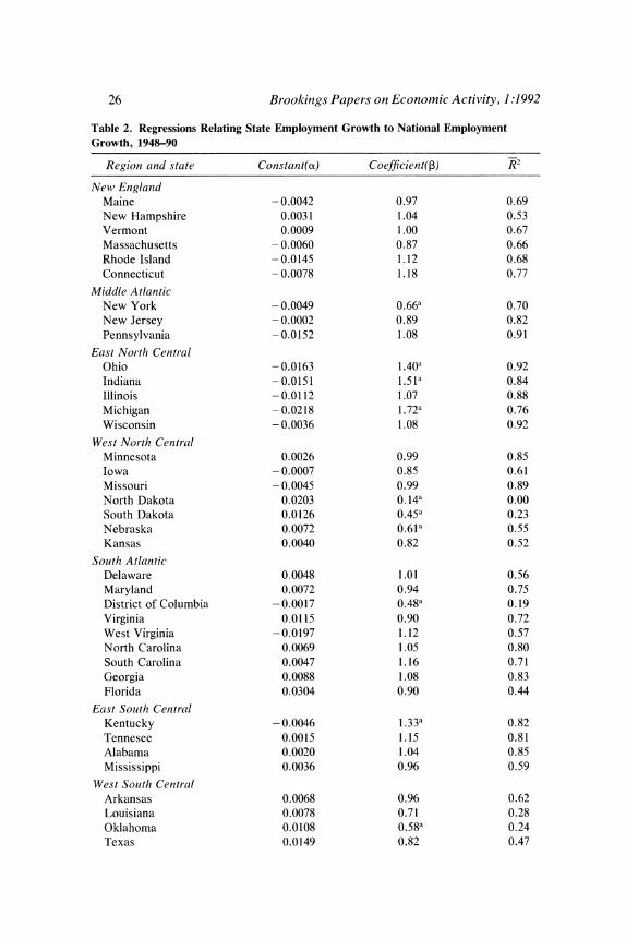
Table 2. Regressions Relating State Employment Growth to National Employment Growth, 1948-90
Region and state Constant(cx) Coefficient(3 )
NewX Englanid Maine - 0.0042 0.97 0.69 New Hampshire 0.0031 1.04 0.53 Vermont 0.0009 1.00 0.67 Massachusetts -0.0060 0.87 0.66 Rhode Island - 0.0145 1.12 0.68 Connecticut - 0.0078 1.18 0.77
Middle Atlantic New York - 0.0049 0.66a 0.70 New Jersey -0.0002 0.89 0.82 Pennsylvania -0.0152 1.08 0.91
East North Central Ohio - 0.0163 1 40a 0.92 Indiana -0.0151 1.51a 0.84 Illinois - 0.0112 1.07 0.88 Michigan -0.0218 1. 72a 0.76 Wisconsin -0.0036 1.08 0.92
West Nor-th Centrcal Minnesota 0.0026 0.99 0.85 Iowa - 0.0007 0.85 0.61 Missouri - 0.0045 0.99 0.89 North Dakota 0.0203 0.14a 0.00 South Dakota 0.0126 0.45a 0.23 Nebraska 0.0072 0.61a 0.55 Kansas 0.0040 0.82 0.52
Solth Atlantic Delaware 0.0048 1.01 0.56 Maryland 0.0072 0.94 0.75 District of Columbia -0.0017 0.48a 0.19 Virginia 0.0115 0.90 0.72 West Virginia -0.0197 1.12 0.57 North Carolina 0.0069 1.05 0.80 South Carolina 0.0047 1.16 0.71 Georgia 0.0088 1.08 0.83 Florida 0.0304 0.90 0.44
East Soutth Central Kentucky -0.0046 1.33a 0.82 Tennesee 0.0015 1.15 0.81 Alabama 0.0020 1.04 0.85 Mississippi 0.0036 0.96 0.59
West South Centr4al Arkansas 0.0068 0.96 0.62 Louisiana 0.0078 0.71 0.28 Oklahoma 0.0108 0.58a 0.24 Texas 0.0149 0.82 0.47
Olivier Jean Blatnclar-d and Lawrence F. Katz 27
Table 2. (Continued)
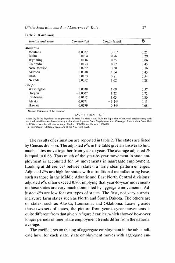
Regioni and state Constant((x) Coefficieit(p) R2
Moluntain Montana 0.0072 0.5 la 0.25 Idaho 0.0104 0.76 0.29 Wyoming 0.0116 0.55 0.06 Colorado 0.0173 0.82 0.43 New Mexico 0.0252 0.50 0.16 Arizona 0.0318 1.04 0.43 Utah 0.0153 0.81 0.54 Nevada 0.0352 1.02 0.28
Pacific Washington 0.0038 1.09 0.57 Oregon - 0.0007 1.22 0.72 California 0.0112 1.03 0.80 Alaska 0.0771 -1.24a 0.13 Hawaii 0.0299 0.34a 0.08
Source: Estimates of the equation
ANi, + PAN, + Oi,, where Ni, is the logarithm of employment in state i at time t, and N, is the logarithm of national employment; both are total establishment-based nonagricultural employment from E,nployment anid Earnlinzgs. Annual data from 1948 to 1990 are used for all states except Alaska (1961-90) and Hawaii (1956-90).
a. Significantly different from one at the 5 percent level.
The results of estimation are reported in table 2. The states are listed by Census division. The adjusted R2s in the table give an answer to how much states move together from year to year. The average adjusted R2 is equal to 0.66. Thus much of the year-to-year movement in state em- ployment is accounted for by movements in aggregate employment. Looking at differences between states, a fairly clear pattern emerges. Adjusted R2s are high for states with a traditional manufacturing base, such as those in the Middle Atlantic and East North Central divisions; adjusted R2s often exceed 0.80, implying that year-to-year movements in those states are very much dominated by aggregate movements. Ad- justed R2s are low for two types of states. The first, not very surpris- ingly, are farm states such as North and South Dakota. The others are oil states, such as Alaska, Louisiana, and Oklahoma. Leaving aside those two sets of states, the picture from year-to-year movements is quite different from that given in figure 2 earlier, which showed how over longer periods of time, state employment trends differ from the national average.
The coefficients on the log of aggregate employment in the table indi- cate how, for each state, state employment moves with aggregate em-
28 Br ookings Paper-s on Economic Activity, 1:1992
ployment. Here, obviously, the proper weighted average is equal to one; of interest is the distribution of Ps across states. Thirteen states have elasticities significantly different from 1. On the high side are manufac- turing states, producing durables such as cars, which have a high elastic- ity with respect to aggregate fluctuations. This is the case for Michigan and Indiana, which have elasticities of 1.72 and 1.51, respectively. On the low side (again, not surprisingly) are farm states and oil states: North Dakota and South Dakota have elasticities of 0.14 and 0.45, respec- tively. From 1961 to 1990, the period for which we have data, Alaska has an elasticity of - 1.24!
Within the context of equation 7, we also explored a number of hypotheses that regularly surface in discussions of regional fortunes. Given that we found little evidence in support of these hypotheses, we shall merely summarize these results in words.
A frequently mentioned hypothesis is that the share of tradables in total production has declined over time and that states are thus less de- pendent on aggregate fluctuations. We thus tested whether the strength of the relation between aggregate employment and state employment has declined over time. We did so by splitting the sample into pre-1970 and post- 1970 components and comparing R2s for the pre- and post- 1970 samples for each state. There was no evidence of a decrease in R2s.
We explored whether the response of state employment was different for some states with respect to increases and decreases in aggregate em- ployment. We found no such evidence, except for Alaska, where both decreases and increases in aggregate employment were associated, dur- ing the sample period, with increases in employment in Alaska. This clearly reflects the fact that Alaska did well during the two oil shock re- cessions.
We explored the idea that aggregate recessions have stronger adverse effects on those states that are already experiencing adverse idiosyn- cratic shocks. Such a hypothesis has most recently emerged in connec- tion with the depth of the current slump in Massachusetts. We thus al- lowed for a different effect of increases and decreases in aggregate employment on state employment and for the coefficients on those in- creases and decreases to depend on the lagged state unemployment rate. We found no evidence in favor of such a hypothesis-no consistent pat- tern in the coefficients on the interaction terms over states or Census divisions. The effect is of the wrong sign and significant for New Eng-
Olivier Jean Blanchard and Lawrence F. Katz 29
land, of the right sign and significant for Mountain and Pacific divisions, and insignificant elsewhere.
The choice we face in the rest of the paper is whether to construct state-specific variables as simple log differences, or as (-differences, us- ing either a common set of estimated Ps for all variables or using Ps esti- mated for each variable (employment as above, unemployment, wages, and so on). Given that for most states, an elasticity of 1 is not rejected by the data, we use simple log differences as measures of state-specific or relative variables in the remainder of the paper. We have checked the robustness of many of our results using (-differences, instead; we found that the results were not very sensitive to the choice of simple log differ- ences or (-differences. For example, the univariate relative employ- ment processes examined earlier are quite similar for simple log differ- ences and for (-differences using the estimated Ps reported in table 2.
The final issue we consider in this section is that of the correlation of state-specific movements in employment within Census divisions or regions. If most of the variation in state relative employment move- ments were common to states in a Census division, then not much would be gained by working with the 51 states individually, rather than with divisions directly. We thus examined the share of the variation in annual state relative employment changes that is common to broader regions. We ran pooled regressions for the 51 states for the 1948 to 1990 period on a full set of region-year interaction dummy variables for regions defined either as Census division or region. The regressions indicate that about 38 percent of annual state relative employment variation is common to Census divisions and about 26 percent is common to Census regions. We conclude from these regressions that the majority of state employment variation is idiosyncratic (after accounting for common national fluctu- ations) and that examining individual states is a fruitful approach. We now turn to characterizing state-specific fluctuations.
Employment, Unemployment, and Participation
Our model implies and the evidence supports the notion that trends in employment do not lead to trends in unemployment. However, a cor- relation may exist between employment trends and average unemploy- ment rates. We first briefly examine whether such a correlation exists;
30 Brookings Papers on Economic Activity, 1:1992
no clear pattern emerges. We then turn to the characterization of the joint fluctuations of employment, unemployment, and participation.
Average Unemployment and Employment Growth Rates
In our model the correlation between mean unemployment rates and employment growth rates depends on the relative importance of the un- derlying sources of growth. It implies that if growth comes from labor demand, a negative correlation should occur between average unem- ployment and employment growth; the opposite should hold if growth comes from labor supply caused by workers' migration. As we pointed out already, our model is likely to be too simple here. Clearly, the equi- librium level of unemployment also depends on the industrial composi- tion of nonfarm production and on the share of agricultural employment. Clearly also, richer and more realistic formalizations of migration be- havior may lead to "wait unemployment," and thus to a positive corre- lation between unemployment and employment growth even when de- mand trends dominate: workers may prefer to be unemployed in a state in which many vacancies occur and high wages prevail, because work- ers' expected future earnings would be higher at any unemployment rate.32
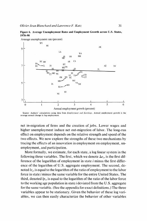
The evidence is given in figure 6, which plots average unemployment rates versus employment growth rates for the period 1970-90.'No clear pattern emerges. The slope of the regression line is equal to - 0.06, with a t statistic of 0.04. The clustering of some states is of interest. The low employment growth states of the Rust Belt have high unemployment rates. Three out of the four states with very high growth rates-Arizona, Florida, and Nevada-have unemployment rates close to the national mean. The farm states have low unemployment rates. While one could explore those relations further, we do not. Instead, we turn to the dy- namic effects of shocks.
Dynamic Responses
Our model points out that two adjustment mechanisms come into play in response to an adverse shock in demand. Lower wages induce
32. This line of reasoning traces back to the Harris-Todaro model of unemployment and has recently been explored under the heading of wait unemployment.
Olivier Jean Blanchard and Law)rence F. Katz 31
Figure 6. Average Unemployment Rates and Employment Growth across U.S. States, 1970-90 Average unemployment rate (percent)
WV MI AK
9 LA
WA AL OR NM
MS
DC OH AR CA PA N..-IL IN KY 7 NY * *-IL IN METN AZ NV
NJ MI t- ?_ , IP -2 -FL RI M1 LGA -
MACT MO WI HI . CO VT TX- *CO
OK ND NC *UT
MN WY 5 IA VA NH
KS- -
SD NE
3 I l 0 1 2 3 4 5 6
Annual employment growth (percent)
Source: Authors' calculations using data from Emnployment anid Earninigs. Annual employment growth is the average annual change in log employment.
net in-migration of firms and the creation of jobs. Lower wages and higher unemployment induce net out-migration of labor. The long-run effect on employment depends on the relative strength and speed of the two effects. We now explore the strengths of these two mechanisms by tracing the effects of an innovation in employment on employment, un- employment, and participation.
More formally, we estimate, for each state, a log linear system in the following three variables. The first, which we denote \ei, is the first dif- ference of the logarithm of employment in state i minus the first differ- ence of the logarithm of U.S. aggregate employment. The second, de- noted lei, is equal to the logarithm of the ratio of employment to the labor force in state i minus the same variable for the entire United States. The third, denoted Ipi, is equal to the logarithm of the ratio of the labor force to the working age population in state i deviated from the U.S. aggregate for the same variable. (See the appendix for exact definitions.) The three variables appear to be stationary. Given the behavior of these log vari- ables, we can then easily characterize the behavior of other variables
32 Br-ookings Papers on Economic Activity, 1:1992
such as the unemployment rate and the participation rate, or changes in the numbers of workers employed, unemployed, or out of the labor force.33 We estimate
eit= otilO + xi, I (L) A 1ei,t- I+ 0ti12 (L) lei,t- I + (Xic3 (L) lip t - I + f iet
= ?i2O + 0Xi21 (L) \eit + oi22 (L) lei,t- + Oti23 (L) 1pipt- I+ Ei,t,
Pit =t i3O + ti31 (L) Aeit + Oi32 (L) lei,t- 1 + Ot33 (L) 'Pi,t- 1 + Eipt
We allow for two lags for each variable. Our approach to estimating this and other systems below is to first estimate them separately for each state, then to do pooled estimation, first by pooling states within Census divisions, then by pooling all states together, allowing in each case for state-fixed effects-that is, state-specific constant terms in each equa- tion. This gives a sense of both commonalities and differences across states.34 In some cases, however, the time dimension is too small to allow for reliable estimation for each state. This is the case here. Our estimation period is limited by the unavailability of information on labor force participation rates from the Current Population Survey (CPS) for most states prior to 1976. Since we include two lags of each variable, we can estimate the system only over the 1978 to 1990 period. In such cases, we perform our estimates only at the Census division and U.S. national levels.3
Our specification of the lag structure, allowing for current changes in \eit to affect current values of leit and Ipit, but not vice versa, and our
33. The unemployment and participation rates are obtained for example using the rela- tions d(U/L) =(E/L)(dln(L/E)) and d(L/P) = (L/P)(dln(L/P)), where U, L, E, and P are unemployment, the labor force, employment, and working age population, respectively. The mean value for the sample of EIL is 0.936; for LIP, it is 0.655.
34. We also have experimented with alternative weighting schemes in our estimates of models pooled across groups of states. We have run unweighted ordinary least squares (OLS) regressions and regressions in which observations for each state are weighted by the level of state employment or population in a base year. Although our unit of observa- tion is a state, one might worry that unweighted OLS results place too much emphasis on small states relative to their importance to the national economy. Because it turns out that our estimates are rather insensitive to whether we do or do not weight by some measure of state size, we report only estimates of the unweighted models.
35. We also have estimated the bivariate system in the first two variables, dropping the third; this requires only data on unemployment and employment and allows estimation using data from 1970 to 1990. The estimated impulse responses for employment and unem- ployment from the bivariate system are nearly identical to those estimated from the trivari- ate system.
Olivier Jean Blanchard and Lawrence F. Katz 33
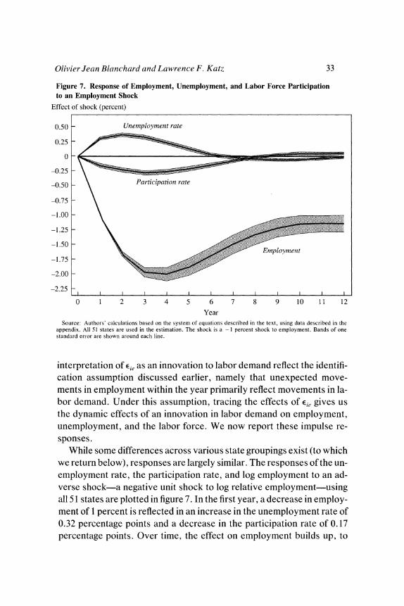
Figure 7. Response of Employment, Unemployment, and Labor Force Participation to an Employment Shock
Effect of shock (percent)
0.50 - Unemployment rate
0.25 -
0 M
-025 - "
-0.50 - Participation tate
-0.75 -
-1.00
-1.25
-1.50 - \ ~~~~~~~~~~~Emplovnieztt
-1.75 -
-2.00 -
-2.25 F l l l l l l l l l l
0 1 2 3 4 5 6 7 8 9 10 I 1 12
Year Source: Authors' calculations based on the system of equations described in the text, using data described in the
appendix. All 51 states are used in the estimation. The shock is a - I percent shock to employment. Bands of one standard error are shown around each line.
interpretation Of E,e as an innovation to labor demand reflect the identifi- cation assumption discussed earlier, namely that unexpected move- ments in employment within the year primarily reflect movements in la- bor demand. Under this assumption, tracing the effects of Eie gives us the dynamic effects of an innovation in labor demand on employment, unemployment, and the labor force. We now report these impulse re- sponses.
While some differences across various state groupings exist (to which we return below), responses are largely similar. The responses of the un- employment rate, the participation rate, and log employment to an ad- verse shock-a negative unit shock to log relative employment-using all 51 states are plotted in figure 7. In the first year, a decrease in employ- ment of 1 percent is reflected in an increase in the unemployment rate of 0.32 percentage points and a decrease in the participation rate of 0.17 percentage points. Over time, the effect on employment builds up, to
34 Brookings Papers on Economic Activity, 1:1992
reach a peak of - 2.0 percent after four years and a plateau of about - 1.3 percent. The effects on unemployment and participation steadily decline and disappear after five to seven years.36
Instead of reporting results in terms of changes in unemployment and participation rates, we can report them in terms of changes in numbers of workers. A decrease in employment of 1 worker in the initial year is associated with an increase in unemployment of 0.3 workers, a decrease in participation of 0.05 workers, and thus an implied increase in net out- migration of 0.65 workers.37 The substantial role played by net migration even in the first year of a shock is similar to the findings of Susan House- man and Katharine Abraham for state-level data in models that ignore the dynamic effects of shocks.38 By five to seven years, the employment response consists entirely of the migration of workers.39
Okun's Coefficients and Shocks to Labor Demand and Supply
As we discussed earlier, comparisons across states give us a way of informally checking our identification assumption. Border states are
36. In general, our results are consistent with previous studies, as summarized in Bar- tik (1991). Our conclusions differ somewhat from Bartik's, who, using data from MSAs, concludes that employment shocks have a small but nonzero, hysteretic effect on unem- ployment. While hysteresis is an idea we sometimes like, we find the conclusion implausi- ble in this case. The result that positive state relative employment shocks permanently affect state relative unemployment is difficult to reconcile with the lack of a clear relation between average employment growth and unemployment rates for U.S. states over our sample period.
37. This may be an overestimate of the initial contribution of migration to adjustment because we are using establishment data on employment. Part of the initial employment response may reflect changes in dual job holding. Changes in the rate of dual job holding will alter the level of employment as measured in the establishment survey, but will not affect the number of unemployed and nonparticipants measured in the household survey. The implied initial migration response to an employment shock is somewhat smaller (0.40 as opposed to 0.65 of the initial adjustment) when we estimate our trivariate system using CPS household employment data, rather than establishment data. However, the implied relative importance of migration is quite similar within several years after a shock.
38. Houseman and Abraham (1990). 39. The lack of a permanent effect of employment shocks on the participation rate does
not rule out the possibility that some workers both do not migrate and permanently drop out of the labor force in response to an adverse demand shock. For example, part of the observed initial reduction in the participation rate from an adverse shock may reflect older workers who take early retirement and permanently drop out of the labor force. The lack of a participation response by seven years after the shock indicates that these workers would have retired anyway by that time, even without an adverse shock.
Olivier Jean Blanchard and Lawrence F. Katz 35
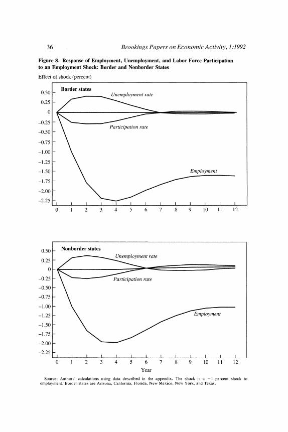
likely to have a larger variance of migration shocks than nonborder states. While shocks to labor demand are likely to generate a negative contemporaneous correlation of employment and unemployment re- sponses, migration shocks are likely instead to generate a positive corre- lation between the two. Thus if migration shocks are quantitatively im- portant for border states and if migration shocks show up in employment within the year, one would expect the estimated response of unemploy- ment to employment to be closer to zero, or even to be positive if supply shocks dominate. Thus we estimate separately the response of unem- ployment and employment for border states (Arizona, California, Flor- ida, New Mexico, New York, and Texas) on the one hand, and all other states on the other. The two sets of responses are plotted in figure 8 and are surprisingly similar. This suggests that even in the border states, mi- gration shocks account for a small proportion of year-to-year employ- ment movements and/or that migration shocks are only partially re- flected in changes in establishment (nonagricultural) employment within the year.40 Similarly distinguishing between farm and nonfarm states, or oil and nonoil states, does not yield obvious differences.
Going beyond the narrow question of identification, are there states where the "Okun coefficient"-the negative of the ratio of the response of unemployment to employment-is substantially lower than the na- tional average?41 To answer this question, we examine the Okun coeffi- cients implied by the estimates of the trivariate system from 1978 to 1990 for individual states and for groups of states (in systems with fixed ef- fects for each state). Keep in mind that when estimating state by state, we have very few degrees of freedom. The estimated Okun coefficient is closer to zero in the farm states ( - 0.22 with a t statistic of 8.1) than in the typical state ( - 0.32 with a t statistic of 17.5 in a regression pooled across all states). In estimates for individual states, we find the Okun co- efficient to be quite low for Mississippi (- 0.01), Nebraska (- 0.09), and Arizona (- 0.14). It is of the wrong sign in Tennessee (0.01), California (0.02), Montana (0.04), Colorado (0.05), South Carolina (0.06), Minne-
40. However, the results vary across individual border states. As we indicate below, two states, Arizona and California, have estimated positive effects of employment on un- employment, suggesting the importance of migration shocks.
41. The use of the expression "Okun coefficient" is not quite correct because Okun introduced his coefficient to characterize the relation between changes in output and changes in unemployment. See Okun (1962).
36 Br ookings Papers on Economic Activity, 1:1992
Figure 8. Response of Employment, Unemployment, and Labor Force Participation to an Employment Shock: Border and Nonborder States
Effect of shock (percent)
Border states U employym ent rate
0
-0.25 Unmlyetrt
-0.25 Participation rate -0.50 -
-0.75 -
-1.00 -
-1.25-
-1.50 - Employment
-1.75 -
-2.00-
-2.25 ll 0 1 2 3 4 5 6 7 8 9 10 11 12
0.50 e Nonborder states
0.25 - Uninlonitt r-ate
-0.25 - Prticipation reate
-0.50 -\
-0.75 -\
-1.00 - \
-1.75 - \~=
-2.25_
0 1 2 3 4 5 6 7 8 9 10 l 1 12
Year
Source: Authors' calculations using data described in the appendix. The shock is a - I percent shock to employment. Border states are Arizona, California, Florida, New Mexico, New York, and Texas.
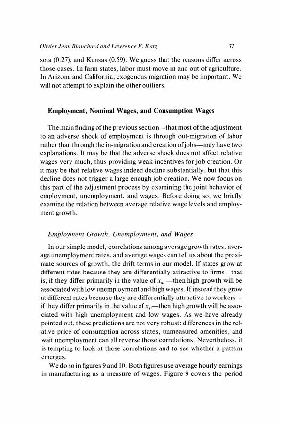
Olivier Jean Blanchard and Lawrence F. Katz 37
sota (0.27), and Kansas (0.59). We guess that the reasons differ across those cases. In farm states, labor must move in and out of agriculture. In Arizona and California, exogenous migration may be important. We will not attempt to explain the other outliers.
Employment, Nominal Wages, and Consumption Wages
The main finding of the previous section-that most of the adjustment to an adverse shock of employment is through out-migration of labor rather than through the in-migration and creation ofjobs-may have two explanations. It may be that the adverse shock does not affect relative wages very much, thus providing weak incentives for job creation. Or it may be that relative wages indeed decline substantially, but that this decline does not trigger a large enough job creation. We now focus on this part of the adjustment process by examining the joint behavior of employment, unemployment, and wages. Before doing so, we briefly examine the relation between average relative wage levels and employ- ment growth.
Employment Growth, Unemployment, and Wages
In our simple model, correlations among average growth rates, aver- age unemployment rates, and average wages can tell us about the proxi- mate sources of growth, the drift terms in our model. If states grow at different rates because they are differentially attractive to firms-that is, if they differ primarily in the value of Xdi -then high growth will be associated with low unemployment and high wages. If instead they grow at different rates because they are differentially attractive to workers- if they differ primarily in the value of xs,-then high growth will be asso- ciated with high unemployment and low wages. As we have already pointed out, these predictions are not very robust: differences in the rel- ative price of consumption across states, unmeasured amenities, and wait unemployment can all reverse those correlations. Nevertheless, it is tempting to look at those correlations and to see whether a pattern emerges.
We do so in figures 9 and 10. Both figures use average hourly earnings in manufacturing as a measure of wages. Figure 9 covers the period
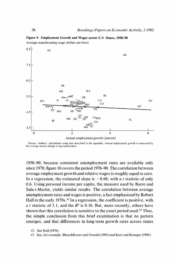
38 Brookings Paper-s on Economic Activity, 1:1992
Figure 9. Employment Growth and Wages across U.S. States, 1950-90
Average manufacturing wage (dollars per hour)
8.5- DC
AK
7.5 -
6.5 -
MI
OH WA
5.5 - IN-. .MT OR HI
WV IL IA LI~~ CA NV
FA-w ; N ) e14 AZ
VT
RI ME SD TN VANM FL RI ~~~~GA
ARSC 3.5 - MS NC
0 4 6
Annual employment growth (percent)
Source: Authors' calculations using data described in the appendix. Annual employment growth is measured by the average annual change in log employment.
1950-90; because consistent unemployment rates are available only since 1970, figure 10 covers the period 1970-90. The correlation between average employment growth and relative wages is roughly equal to zero. In a regression, the estimated slope is - 0.68, with a t statistic of only 0.6. Using personal income per capita, the measure used by Barro and Sala-i-Martin, yields similar results. The correlation between average unemployment rates and wages is positive, a fact emphasized by Robert Hall in the early 1970s.42 In a regression, the coefficient is positive, with a t statistic of 3. 1, and the R2 is 0.16. But, more recently, others have shown that this correlation is sensitive to the exact period used.43 Thus, the simple conclusion from this brief examination is that no pattern emerges, and that differences in long-term growth rates across states
42. See Hall (1970). 43. See, for example, Blanchflower and Oswald (1991) and Katz and Krueger (1991).
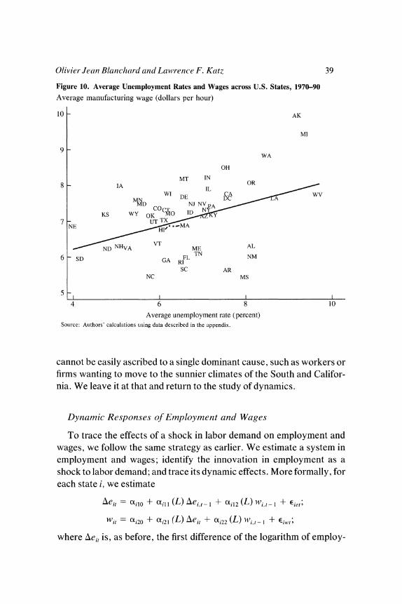
Olivier Jean Blanchard and Lawrence F. Katz 39
Figure 10. Average Unemployment Rates and Wages across U.S. States, 1970-90
Average manufacturing wage (dollars per hour)
10 AK
MI
9 WA
OH
MT IN OR
| ~ ~ ~ ~ W CAc WV
7NE M
NNHA VT
ME AL
6 SD GA RI NM
SC AR NC MS
5 I I l 4 6 8 10
Average unemployment rate (percent) Source: Authors' calculations using data described in the appendix.
cannot be easily ascribed to a single dominant cause, such as workers or firms wanting to move to the sunnier climates of the South and Califor- nia. We leave it at that and return to the study of dynamics.
Dynamic Responses of Employment and Wages
To trace the effects of a shock in labor demand on employment and wages, we follow the same strategy as earlier. We estimate a system in employment and wages; identify the innovation in employment as a shock to labor demand; and trace its dynamic effects. More formally, for each state i, we estimate
eit= otilO + otill (L) z\ei,- + Otil2 (L) li,t-1 + 'iet;
Wit= ti2O + Oti21 (L) leit + Oi22 (L) "i ,- I + Filt;
where leit is, as before, the first difference of the logarithm of employ-
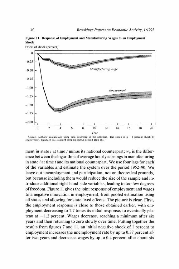
40 Brookings Papers on Economic Activity, 1:1992
Figure 11. Response of Employment and Manufacturing Wages to an Employment Shock Effect of shock (percent)
0
-0.25
-0.50 - Manzufactut-ing wage
-0.75 -
-1.00 \ ~~~~~~~~~Employment
-1.25 -
-1.50
-1.75-
-2.00 -
0 2 4 6 8 10 12 14 16 18 20
Year Source: Authors' calculations using data described in the appendix. The shock is a - I percent shock to
employment. Bands of one standard error are shown around each line.
ment in state i at time t minus its national counterpart; wit is the differ- ence between the logarithm of average hourly earnings in manufacturing in state i at time t and its national counterpart. We use four lags for each of the variables and estimate the system over the period 1952-90. We leave out unemployment and participation, not on theoretical grounds, but because including them would reduce the size of the sample and in- troduce additional right-hand-side variables, leading to too few degrees of freedom. Figure 11 gives the joint response of employment and wages to a negative innovation in employment, from pooled estimation using all states and allowing for state fixed effects. The picture is clear. First, the employment response is close to those obtained earlier, with em- ployment decreasing to 1.7 times its initial response, to eventually pla- teau at - 1.2 percent. Wages decrease, reaching a minimum after six years and then returning to zero slowly over time. Putting together the results from figures 7 and 11, an initial negative shock of 1 percent to employment increases the unemployment rate by up to 0.37 percent af- ter two years and decreases wages by up to 0.4 percent after about six
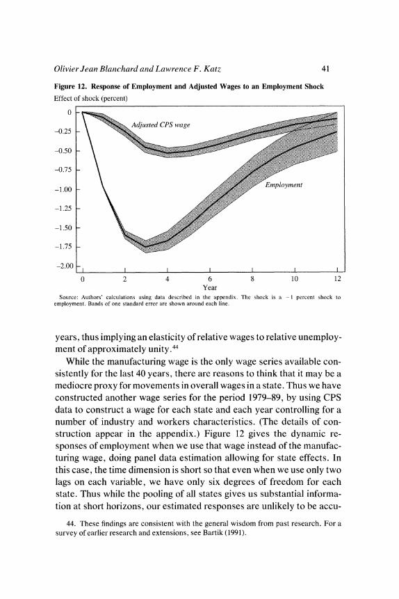
Olivier Jean Blanchard and Lawrence F. Katz 41
Figure 12. Response of Employment and Adjusted Wages to an Employment Shock
Effect of shock (percent)
0
-0.25
-0.50-
-0.75-
SO f X >t Emp~~~~~~~~~~loyment
-1.00
-1.25-
-1.50-
-1.75 -
-2.00 _ I I I I I I
0 2 4 6 8 10 12 Year
Source: Authors' calculations using data described in the appendix. The shock is a - I percent shock to employment. Bands of one standard error are shown around each line.
years, thus implying an elasticity of relative wages to relative unemploy- ment of approximately unity.44
While the manufacturing wage is the only wage series available con- sistently for the last 40 years, there are reasons to think that it may be a mediocre proxy for movements in overall wages in a state. Thus we have constructed another wage series for the period 1979-89, by using CPS data to construct a wage for each state and each year controlling for a number of industry and workers characteristics. (The details of con- struction appear in the appendix.) Figure 12 gives the dynamic re- sponses of employment when we use that wage instead of the manufac- turing wage, doing panel data estimation allowing for state effects. In this case, the time dimension is short so that even when we use only two lags on each variable, we have only six degrees of freedom for each state. Thus while the pooling of all states gives us substantial informa- tion at short horizons, our estimated responses are unlikely to be accu-
44. These findings are consistent with the general wisdom from past research. For a survey of earlier research and extensions, see Bartik (1991).
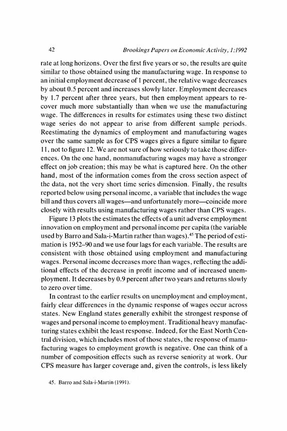
42 Brookings Papers on Economic Activity, 1:1992
rate at long horizons. Over the first five years or so, the results are quite similar to those obtained using the manufacturing wage. In response to an initial employment decrease of 1 percent, the relative wage decreases by about 0.5 percent and increases slowly later. Employment decreases by 1.7 percent after three years, but then employment appears to re- cover much more substantially than when we use the manufacturing wage. The differences in results for estimates using these two distinct wage series do not appear to arise from different sample periods. Reestimating the dynamics of employment and manufacturing wages over the same sample as for CPS wages gives a figure similar to figure 1 1, not to figure 12. We are not sure of how seriously to take those differ- ences. On the one hand, nonmanufacturing wages may have a stronger effect on job creation; this may be what is captured here. On the other hand, most of the information comes from the cross section aspect of the data, not the very short time series dimension. Finally, the results reported below using personal income, a variable that includes the wage bill and thus covers all wages-and unfortunately more-coincide more closely with results using manufacturing wages rather than CPS wages.
Figure 13 plots the estimates the effects of a unit adverse employment innovation on employment and personal income per capita (the variable used by Barro and Sala-i-Martin rather than wages).45 The period of esti- mation is 1952-90 and we use four lags for each variable. The results are consistent with those obtained using employment and manufacturing wages. Personal income decreases more than wages, reflecting the addi- tional effects of the decrease in profit income and of increased unem- ployment. It decreases by 0.9 percent after two years and returns slowly to zero over time.
In contrast to the earlier results on unemployment and employment, fairly clear differences in the dynamic response of wages occur across states. New England states generally exhibit the strongest response of wages and personal income to employment. Traditional heavy manufac- turing states exhibit the least response. Indeed, for the East North Cen- tral division, which includes most of those states, the response of manu- facturing wages to employment growth is negative. One can think of a number of composition effects such as reverse seniority at work. Our CPS measure has larger coverage and, given the controls, is less likely
45. Barro and Sala-i-Martin (1991).
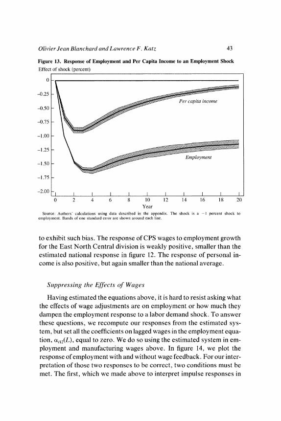
Olivier Jean Blanchard and Lawrenice F. Katz 43
Figure 13. Response of Employment and Per Capita Income to an Employment Shock
Effect of shock (percent)
0
-0.25
-050 L5 ~~~~~~~~~~~~~~~Per capita iticottie -0.50-
-0.75-
-1.00 -
-1.25
\ ~~~~~~~~~~
~~Emiploymentt -1.50
-1.75
-2.00
0 2 4 6 8 10 12 14 16 18 20 Year
Source: Authors' calculations using data described in the appendix. The shock is a - I percent shock to employment. Bands of one standard error are shown around each line.
to exhibit such bias. The response of CPS wages to employment growth for the East North Central division is weakly positive, smaller than the estimated national response in figure 12. The response of personal in- come is also positive, but again smaller than the national average.
Suppressing the Effects of Wages
Having estimated the equations above, it is hard to resist asking what the effects of wage adjustments are on employment or how much they dampen the employment response to a labor demand shock. To answer these questions, we recompute our responses from the estimated sys- tem, but set all the coefficients on lagged wages in the employment equa- tion, UM12(L), equal to zero. We do so using the estimated system in em- ployment and manufacturing wages above. In figure 14, we plot the response of employment with and without wage feedback. For our inter- pretation of those two responses to be correct, two conditions must be met. The first, which we made above to interpret impulse responses in
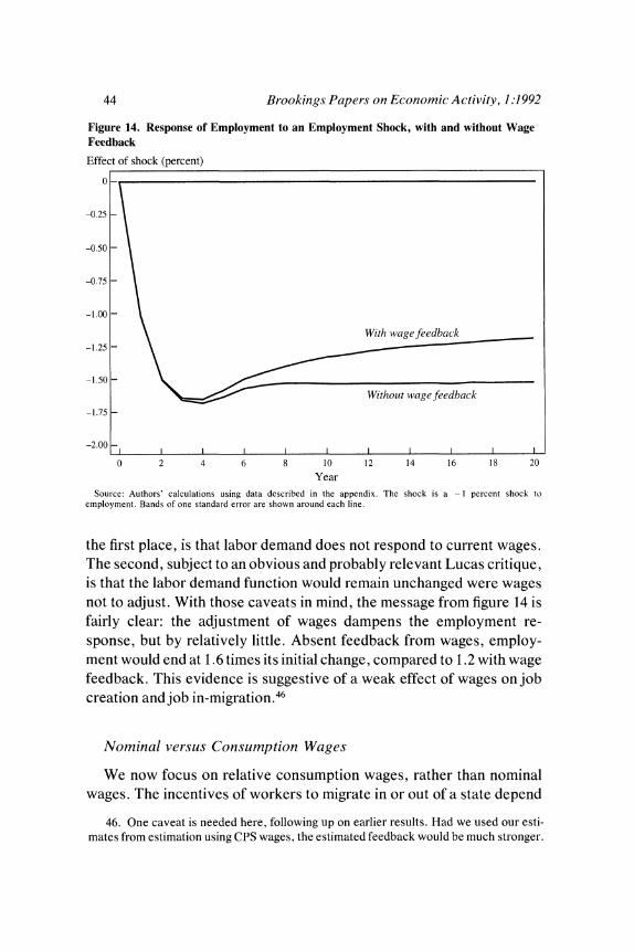
44 Brookings Papers on Economic Activity, 1:1992
Figure 14. Response of Employment to an Employment Shock, with and without Wage Feedback
Effect of shock (percent)
0 -0.25 -
-0.50 -
-0.75 -
-1.00 -
\ ~~~~~~~~~With wagefeedback -1.25 -
-1.50 -
-1.75 -
-2.00 - I I
0 2 4 6 8 10 12 14 16 18 20
Year Source: Authors' calculations using data described in the appendix. The shock is a - I percent shock to
employment. Bands of one standard error are shown around each line.
the first place, is that labor demand does not respond to current wages. The second, subject to an obvious and probably relevant Lucas critique, is that the labor demand function would remain unchanged were wages not to adjust. With those caveats in mind, the message from figure 14 is fairly clear: the adjustment of wages dampens the employment re- sponse, but by relatively little. Absent feedback from wages, employ- ment would end at 1.6 times its initial change, compared to 1.2 with wage feedback. This evidence is suggestive of a weak effect of wages on job creation and job in-migration.46
Nominal versus Consumption Wages
We now focus on relative consumption wages, rather than nominal wages. The incentives of workers to migrate in or out of a state depend
46. One caveat is needed here, following up on earlier results. Had we used our esti- mates from estimation using CPS wages, the estimated feedback would be much stronger.
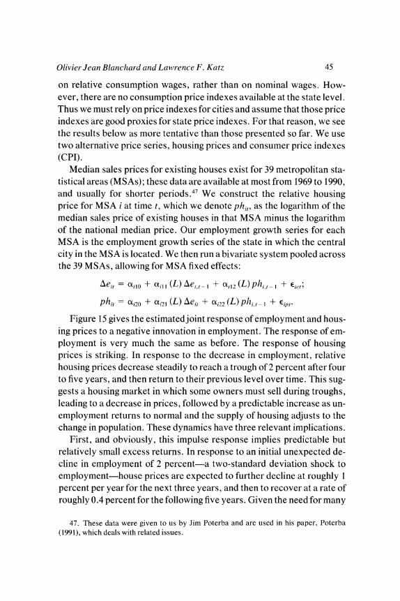
Olivier Jean Blanchard and Lawrence F. Katz 45
on relative consumption wages, rather than on nominal wages. How- ever, there are no consumption price indexes available at the state level. Thus we must rely on price indexes for cities and assume that those price indexes are good proxies for state price indexes. For that reason, we see the results below as more tentative than those presented so far. We use two alternative price series, housing prices and consumer price indexes (CPI).
Median sales prices for existing houses exist for 39 metropolitan sta- tistical areas (MSAs); these data are available at most from 1969 to 1990, and usually for shorter periods.47 We construct the relative housing price for MSA i at time t, which we denote phi,, as the logarithm of the median sales price of existing houses in that MSA minus the logarithm of the national median price. Our employment growth series for each MSA is the employment growth series of the state in which the central city in the MSA is located. We then run a bivariate system pooled across the 39 MSAs, allowing for MSA fixed effects:
\eit = otilO + till (L) Aei,t- + oil2 (L) phit- + Eiet;
P = hti2O + -i2l (L) eit + ?ti22 (L) phit-I + Eipt
Figure 15 gives the estimated joint response of employment and hous- ing prices to a negative innovation in employment. The response of em- ployment is very much the same as before. The response of housing prices is striking. In response to the decrease in employment, relative housing prices decrease steadily to reach a trough of 2 percent after four to five years, and then return to their previous level over time. This sug- gests a housing market in which some owners must sell during troughs, leading to a decrease in prices, followed by a predictable increase as un- employment returns to normal and the supply of housing adjusts to the change in population. These dynamics have three relevant implications.
First, and obviously, this impulse response implies predictable but relatively small excess returns. In response to an initial unexpected de- cline in employment of 2 percent-a two-standard deviation shock to employment-house prices are expected to further decline at roughly 1 percent per year for the next three years, and then to recover at a rate of roughly 0.4 percent for the following five years. Given the need for many
47. These data were given to us by Jim Poterba and are used in his paper, Poterba (1991), which deals with related issues.
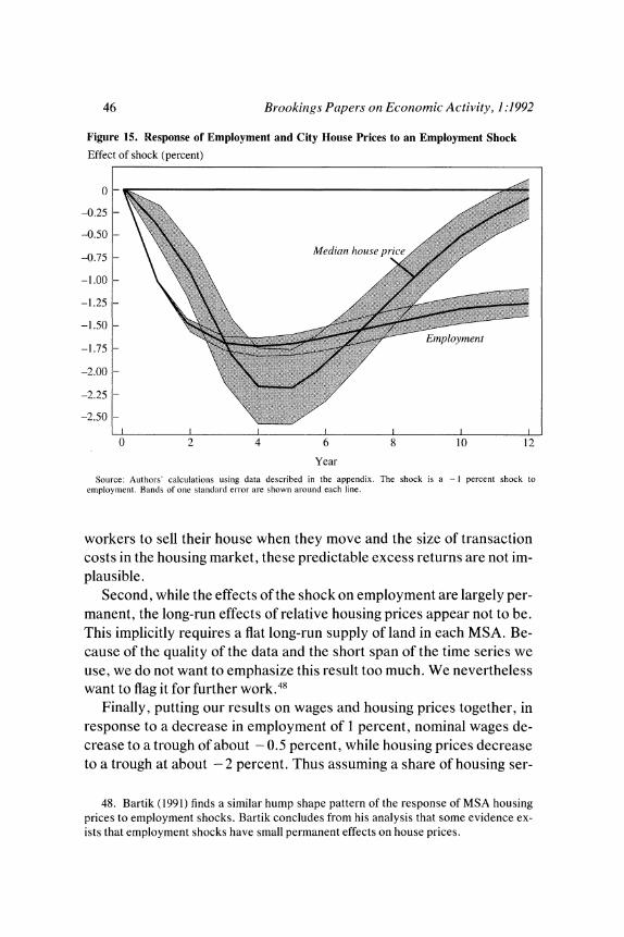
46 Br-ookings Paper-s on Economic Activity, 1:1992
Figure 15. Response of Employment and City House Prices to an Employment Shock
Effect of shock (percent)
O)7 - Median house price *
-1.25 -e
0
-1.50 -
emplymen. Bads o on stadarderro areshon Eruploachente
-1.75rs to-sell their house when they move and the size of transaction
-2.25-
plausible.~ ~ ~ ~~~Mdinhosep'-c
-2.50 -
Secod, wile he ffecs ofthe hoc on mplomentareloymelyn er
0 2 4 6 8 10 12
Year
Source: Authors' calculations using data described in the appendix. The shock is a - I percent shock to
employment. Bands of one standard error are shown around each line.
workers to sell their house when they move and the size of transaction costs in the housing market, these predictable excess returns are not im- plausible.
Second, while the effects of the shock on employment are largely per- manent, the long-run effects of relative housing prices appear not to be. This implicitly requires a flat long-run supply of land in each MSA. Be- cause of the quality of the data and the short span of the time series we use, we do not want to emphasize this result too much. We nevertheless want to flag it for further work.4
Finally, putting our results on wages and housing prices together, in response to a decrease in employment of 1 percent, nominal wages de- crease to a trough of about - 0.5 percent, while housing prices decrease to a trough at about - 2 percent. Thus assuming a share of housing ser-
48. Bartik (1991) finds a similar hump shape pattern of the response of MSA housing prices to employment shocks. Bartik concludes from his analysis that some evidence ex- ists that employment shocks have small permanent effects on house prices.
Oliv'ier Jean Blanchard and Lawrence F. Katz 47
vices of 15 percent and ignoring the fact that the price of other nontrada- bles probably also goes down, consumption wages decrease only by about 0.2 percent, or 40 percent of the decrease in nominal wages. For both renters and house owners, the drop in prices reduces incentives to migrate, but through different channels. In response to an adverse shock, rents are likely to decrease with house prices, dampening the de- cline in renters' consumption wages, and thus the incentive for renters to migrate. For owners, on the other hand, lower housing prices mean a capital loss; if they expect housing prices to pick up again when eco- nomic conditions improve (and our evidence, as well as James Poterba's evidence suggests that this may be rational), those workers may decide to stay rather than to leave and realize a loss.49
We can directly look at the behavior of local CPIs for the 23 MSAs for which they are available for a reasonably long time period. Thus we construct the relative consumer price at time t for MSA i as the logarithm of the CPI for MSA i at time t minus the logarithm of the national coun- terpart. We then estimate a bivariate system in relative consumer prices and employment growth analogous to the one above for the 1968-88 pe- riod. The implied impulse responses of consumer prices and employ- ment to a unit shock to employment are given in figure 16. Consumer prices respond slowly to a shock to employment and eventually de- crease by 0.38 percent after six years in response to an initial 1 percent decrease in employment. The effect on local prices slowly dissipates and is essentially gone after 15 years or so. These responses of overall local prices are fairly consistent with house price changes playing the key role in changes in local prices.50
Altogether, our results imply a small response of real consumption wages in response to relative shocks to employment. These findings re- inforce our view that unemployment rather than relative wages explains the adjustment of the local labor force to changes in labor market condi- tions. A strong response of migration to changes in unemployment and weak sensitivity to wage differentials is consistent with slow conver- gence of wages and income per capita across states and the evidence on
49. Poterba(1991). 50. We report these results with some hesitation. While results from pooled estimation
are sensible, results vary substantially across subsets of MSAs. For example, for MSAs in the East region, we find a negative contemporaneous effect of employment innovations on CPIs.

48 Brookings Papers on Economic Activity, 1:1992
Figure 16. Response of Employment and City Consumer Prices to an Employment Shock
Effect of shock (percent)
-0.25 -
-0.50 Consumer price index
-0.75 -
-1.00
-1.25-
-1.50-
-1.75
-2.00
0 2 4 6 8 10 12 14 16 18 20
Year Source: Authors' calculations using data described in the appendix. The shock is a -I percent shock to
employment. Bands of one standard error are shown around each line.
the weak effect of wage differentials on decadal migration rates found by Barro and Sala-i-Martin.51
The Effects of Observable Demand Shocks
Throughout this paper, we have associated innovations in employ- ment with innovations in labor demand. In this section, we take the al- ternative course of relying on observable shifts in demand. To this end, we construct two variables. Both are plausibly exogenous and move enough to have a noticeable effect on labor demand.
The first is defense spending, or more precisely the real value of mili- tary prime contract awards by state, a variable that has been used by Davis, Loungani, and Mahidhara in a related context (see appendix for
51. Barro and Sala-i-Martin (1991).
Olivier Jean Blanchar-d and Lawrence F. Katz 49
details of construction).52 It exhibits substantial movements across states and time. On average, from 1951 to 1988 (the period for which we can construct the series) it accounts for more than 6 percent of state in- come for four states-California, Connecticut, Massachusetts, and Mis- souri-and the District of Columbia. For those states and the District, the standard deviation of forecast errors from a simple univariate proc- ess is on average equal to 14 percent; some forecast errors exceed 30 percent.
The second variable is a mix variable that gives the employment growth in a state predicted by the growth of its industries nationally; it has been constructed and used by Bartik in a similar context.53 The se- ries is generated for each state and each year, from 1970 to 1989, as a weighted average of the growth rates of national industry employment (aggregated to two-digit SIC categories) with the weights calculated as the previous year share of state employment in each industry. This vari- able will be a valid instrument in a given state if industry national growth rates are uncorrelated with labor supply shocks in the state. This in turn will be true if sectoral employment at the two-digit level is not too con- centrated in any state, a condition that appears satisfied in the data. Be- cause we shall use the deviation of this variable from the national growth rate of employment, this deviation will be a good instrument if states dif- fer sufficiently in their sectoral employment composition. This condi- tion also appears to be satisfied.
In a previous section, we characterized the joint movement in em- ployment and unemployment traced by an innovation in employment.54 Under our identifying assumptions, this innovation reflected only labor demand shocks. The question we ask here is whether the relation be- tween employment and unemployment traced by each of our two ob- servable variables is indeed similar to that characterized before.55 To that end, we specify the following equation:
leit = ?tio + o-il(L) Aeit + Oli2 (L) leit I + E:il(
52. Davis, Loungani, and Mahidhara (1991). 53. Bartik (1991). 54. We shall ignore participation here. 55. One could clearly do more, such as tracing the effects of each of the two variables
on employment, unemployment, wages, and so on. To some extent, this has been done by the authors cited above. But our focus here is in potentially validating our earlier identifi- cation assumption; we limit ourselves to that here.
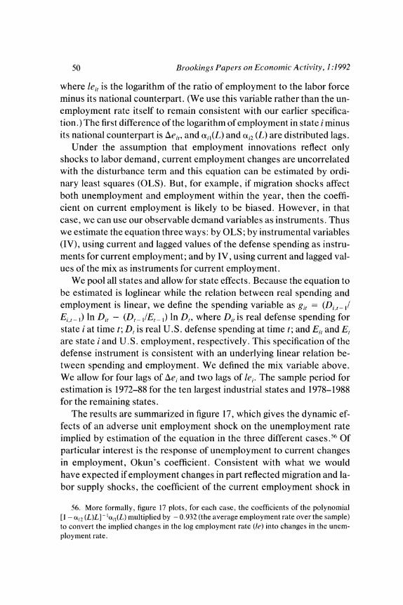
50 Brookings Papers on Economic Activity, 1:1992
where leit is the logarithm of the ratio of employment to the labor force minus its national counterpart. (We use this variable rather than the un- employment rate itself to remain consistent with our earlier specifica- tion.) The first difference of the logarithm of employment in state i minus its national counterpart is leit, and cxil(L) and CXi2 (L) are distributed lags.
Under the assumption that employment innovations reflect only shocks to labor demand, current employment changes are uncorrelated with the disturbance term and this equation can be estimated by ordi- nary least squares (OLS). But, for example, if migration shocks affect both unemployment and employment within the year, then the coeffi- cient on current employment is likely to be biased. However, in that case, we can use our observable demand variables as instruments. Thus we estimate the equation three ways: by OLS; by instrumental variables (IV), using current and lagged values of the defense spending as instru- ments for current employment; and by IV, using current and lagged val- ues of the mix as instruments for current employment.
We pool all states and allow for state effects. Because the equation to be estimated is loglinear while the relation between real spending and employment is linear, we define the spending variable as git = (Di t- I/
Eit - ,) ln Dit - (Dt- I/Et_ I) ln Dt, where Dit is real defense spending for state i at time t; Dt is real U.S. defense spending at time t; and Eit and Et are state i and U.S. employment, respectively. This specification of the defense instrument is consistent with an underlying linear relation be- tween spending and employment. We defined the mix variable above. We allow for four lags of Aei and two lags of lei. The sample period for estimation is 1972-88 for the ten largest industrial states and 1978-1988 for the remaining states.
The results are summarized in figure 17, which gives the dynamic ef- fects of an adverse unit employment shock on the unemployment rate implied by estimation of the equation in the three different cases.56 Of particular interest is the response of unemployment to current changes in employment, Okun's coefficient. Consistent with what we would have expected if employment changes in part reflected migration and la- bor supply shocks, the coefficient of the current employment shock in
56. More formally, figure 17 plots, for each case, the coefficients of the polynomial [1 - cOi2 (L)L] - loxil(L) multiplied by - 0.932 (the average employment rate over the sample) to convert the implied changes in the log employment rate (le) into changes in the unem- ployment rate.
Olivier Jean Blanchard and Lawrence F. Katz 51
Figure 17. Response of Unemployment to an Employment Shock, Ordinary Least Squares and Instrumental Variables Estimates
Effect of shock (percent)
.36 -
IV (inidustty mix)
.30 - OLS
.24-
.18-
.12 -IV (mnilitaty contracts)
.06-
l I I I I I I I I
0 1 2 3 4 5 6 7 8 Year
Source: Authors' calculations using data described in the appendix. The shock is a - I percent shock to employment.
the unemployment equation is slightly larger when we use the industry- mix instrument than when we use OLS. On the other hand, the coeffi- cient is slightly smaller when we use the military contracts instrument. Overall, the shapes of the estimated response of unemployment to an employment shock are rather similar for all three approaches, although the two instrumental variables approaches lead to substantially less pre- cise estimates. We see these results as providing support for our identi- fication assumptions.
Conclusion
Over the postwar period, some U.S. states have consistently grown faster than the national average, while some have grown more slowly. Booms and slumps for states are best described as transitory accelera- tions or slowdowns of employment growth. Growth eventually returns
52 Brookings Papers on Economic Activity, 1:1992
to normal, but the path of employment is permanently affected. These transitory changes in growth lead to transitory fluctuations in relative unemployment and wages. The dominant adjustment mechanism is la- bor mobility, rather than job creation or job migration. Labor mobility, in turn, appears to be primarily a response to changes in unemployment, rather than in consumption wages.
The Case of Massachusetts
It is in this light that one must view the travails of Massachusetts since the early 1980s. Over the postwar period, Massachusetts has been among the states in which relative employment has steadily declined. Employment growth in Massachusetts was below the U.S. rate for all but four years from 1948 to 1979. In the early 1980s, however, a number of industries experienced a boom in demand, and from 1980 to 1985 an- nual employment growth was 2.0 percent-0.6 percent higher than the national average. To many, it appeared that the underlying trend was changing-an occurrence which, as we have documented, does not ap- pear to have happened to more than a couple of states over the postwar period. The unemployment rate, which was equal to the national rate in 1979, stood at 3.6 percent below the national average in 1985. Relative wages in manufacturing, which were 11 percent below the national aver- age in 1979, were only 5 percent below the national average by 1985. CPS wages showed a similar evolution, increasing from about 3 percent below the national average in 1979 to 1 percent above in 1985. Housing prices in Boston increased from 17 percent above the national average in 1979 to 57 percent above the national average in 1985.
By 1985, however, relative employment growth had already turned sharply lower. In every year from 1985 to 1991, employment growth was lower than the national average, averaging - 0.1 percent a year, or about 2.2 percent below the national average. The decline in employment was particularly sharp in 1990 and 1991: - 4 percent and - 6 percent, respec- tively. Relative unemployment increased steadily; by 1991, the unem- ployment rate stood at 2 percent above the national average. Not until 1990 were relative wages in manufacturing stabilized. By then, they had increased another 10 percent from their 1985 value to stand at 5 percent above average. CPS relative wages followed a similar pattern; by 1990, they were 10 percent above the national average. The turnaround in
Olivier Jean Blanchard and Lawrence F. Katz 53
housing prices was faster, with relative housing prices in Boston peaking at 72 percent above the national average in 1987 and decreasing to 60 percent above average in 1990.
The debate in Massachusetts has centered on the question of whether the bust of the late 1980s was caused by the boom of the early 1980s and thus was, in effect, "home grown."57 If the experience of Massachusetts were typical of what we found, the answer would clearly be negative. Our tracing of typical responses did not show signs of oscillations-of movements in wages leading to overshooting of employment responses, or of busts following booms. We would conclude that first, a sharp exog- enous increase in demand occurred in the early 1980s, in particular for minicomputers and various forms of financial services, followed by a sharp exogenous decrease in demand, for roughly the same products, in the late 1980s. We would forecast that Massachusetts would return to normal over the next half decade through a steady increase in net outmi- gration of workers.
However, there are signs that the Massachusetts experience of the 1980s has been atypical. The numbers above about wage and housing price growth appear large; we indicated earlier that the responses of New England states of wages to employment appeared to be stronger than the standard response. Thus we perform a simple exercise: we sim- ulate the response of wages and housing prices to the actual employment path, using the equations estimated above from pooled data; we then compute the prediction errors. We find that manufacturing wage growth from 1979 to 1986 was consistent with the evolution of employment, but substantially exceeded its predicted value after 1986. From 1986 to 1990, actual nominal wage growth was 20 percent, twice its predicted value of 10 percent. Our simulation exercise also shows that housing prices increased much more than in a typical regional boom. From 1979 to 1986, the actual increase in housing prices was 87 percent, compared to a predicted 47 percent. From 1986 to 1990, both the actual and predicted increases were 9 percent. Thus the evidence points to a stronger re- sponse of wages and housing prices than is typically the case and sug- gests that the bust may have been partially caused by the earlier boom. Thus, somewhat unfortunately, the experience that partly motivated our study turns out to be atypical. Further progress on separating the
57. See Sass (1992).
54 Br-ookings Paper-s on Economic Activity, 1:1992
role of the previous boom and of adverse shocks requires a more de- tailed look at disaggregated employment; we do not pursue that here. Instead, we turn to three larger issues raised by our findings.
Is the Adjustment Process Efficient?
We have shown that most of the adjustment of states to shocks is through movements of labor, rather than through job creation orjob mi- gration. U.S. states affected by an adverse shock may find this adjust- ment unappealing. However, if firms' and workers' private costs and benefits of moving reflect social costs and benefits, the adjustment is ef- ficient. Do private costs and benefits reflect social costs and benefits? Many reasons exist to suspect that they do not. Wages may not be re- sponsive enough to labor market conditions, leading to excess unem- ployment and (as our model shows) too large a long-run response of em- ployment to shocks. Liquidity constraints may force workers who become unemployed to leave the state rather than borrow and wait for the upturn, leading to excessive labor out-migration (although we have seen that the behavior of housing prices, which may come from a thin housing market, may induce owners to stay). Increasing fiscal burdens and fiscal crises in states that experience adverse shocks may deter firms from coming, despite lower wages. Our paper, which is largely descrip- tive, cannot answer those questions. However, further, more micro- based work can provide answers and thus give a richer picture of the ad- justment process. Two directions of empirical research strike us as promising. The first is the integration of our results with micro-evidence about who moves and who is left behind.58 The second is a characteriza- tion of the separate responses of job creation and job destruction to shocks. The data base on the distribution of employment changes by es- tablishment compiled by Steven Davis and John Haltiwanger seems well adapted to the task.59
Implications for Growth
We argued earlier that any model of regional fluctuations must be at least consistent with the existence of large differences in rates of growth across states. The model we developed could explain (admittedly in
58. See Topel (1986) and Bartik (1991) for a start. 59. Davis and Haltiwanger (1990). See also Papke (1989).

Olivier Jean Blanchar-d and Lawrence F. Katz 55
black-box fashion) both trends and fluctuations. Our empirical work fo- cused on fluctuations, and our somewhat casual examination of the rela- tion between average growth rates, unemployment rates, and relative wages did not yield any sharp conclusions. Does what we have learned from fluctuations provide hints about trends?
Research on regional growth has focused on this question at two lev- els. The first is whether differences in state growth have been caused primarily by movements of workers, which trigger an inflow of firms, or from movements of firms, which trigger an inflow of workers. In the ter- minology of our model, the first question has been whether growth was primarily caused by differences in x,i or Xdi. The second question is what makes firms or workers prefer one state to another-what lies behind the x's. Focusing on firms, two main hypotheses have been developed. The "footloose" hypothesis holds that the postwar period has been a pe- riod of adjustment; costs of being some distance from major markets or major industrial centers have steadily decreased, inducing firms to move from the old manufacturing regions to the South and the West. The sec- ond hypothesis is that some states have offered industrial structures that have been consistently more conducive to growth. Those states have had young growing industries; have been able to attract new young in- dustries; or simply have been able to attract a steady flow of new firms.60 As a result, these states have been able to grow faster than oth- ers. Our results can shed no light on the second set of issues; that would require more disaggregated data.61 But our results can shed some light on the first. If steady movement of workers to more pleasant regions of the South and West was the causal mechanism, the change would have had to have worked through lower wages resulting from migration of workers, which in turn triggered a movement of firms. However, our analysis shows that the response ofjob creation to movements in wages appears weak. This suggests that the primary cause of differences in em- ployment growth across states is movements of firms, which triggered movements of workers.
Implications for Europe
What are the implications of our findings for those countries that are moving toward a fixed exchange rate zone with few or no barriers to
60. See Miracky (1992). 61. See Glaeser and others (1991) and Garcia-Mila and McGuire (1991).
56 Brookings Papers on Economic Activity, 1:1992
goods and factor mobility? A common argument raised during discus- sions of a common currency area for Europe is that, once the common currency is introduced and exchange rates are thus irrevocably fixed, firms and workers will no longer expect to be bailed out by monetary expansion and depreciation. Faced with a decline in competitiveness, firms will find that wage concessions and productivity improvements will be quicker, leading to a faster return to full employment. The experi- ence of the United States clearly shows the limits of this argument. In response to an adverse shock in demand, relative nominal wages indeed decline, but they do not decline by a large enough amount to prevent in- creases in unemployment. What they trigger is mostly labor out-migra- tion, rather than job in-migration orjob creation.
Furthermore, European countries are likely to remain quite different from U.S. states in a number of ways. First, in the United States, sub- stantial interstate transfers operating through the federal tax and trans- fer system help cushion the impact of regional shocks.62 Such a system of transfers is unlikely to be implemented on the same scale in Europe. Labor mobility across European countries is also likely to remain lower than labor mobility across U.S. states.63 To the extent that labor mobil- ity is the main source of adjustment in the United States, this suggests that shocks will have larger and longer lasting effects on relative unem- ployment in Europe.64 This conclusion must be qualified to allow for the possibility that lower labor mobility in Europe than in the United States may lead to more wage flexibility on the part of workers in Europe than in the United States. Absent this high wage flexibility, our paper thus warns, the adjustment to relative shocks in the European common cur- rency area may turn out to be a painful and protracted process.
62. See Sala-i-Martin and Sachs (1991). 63. Eichengreen (1992) finds that net migration is much less sensitive to shocks to re-
gional wages and unemployment in Italy and Great Britain than in the United States. Houseman and Abraham (1990) find that regional employment shocks generate substan- tially more net migration in the United States than in Germany.
64. The importance of labor mobility for the desirability of common currency areas dates at least back to the work of Mundell (1961).
Olivier Jean Blanchard and Lawrence F. Katz 57
APPENDIX
Description of Data
IN THIS APPENDIX, we describe the state and U.S. aggregate time series used in our paper.
Employment
The basic measure of employment is the establishment-based total nonagricultural employment series, taken from the Bureau of Labor Sta- tistics (BLS) Employment and Earnings. The data range from 1947 to 1990 for the United States as a whole and for all states (except Alaska and Hawaii; their data begin in 1960 and 1955, respectively).
Unemployment and Labor Force Participation Rates
The basic measures of unemployment and participation come from the Current Population Survey (CPS). These series, taken from the BLS Geographic Profile of Employment and Unemployment, are available for all states from 1976 to 1990 and for 10 large states from 1970. Data on unemployment for the other 40 states and the District of Columbia for years prior to 1976 were constructed from BLS unemployment rates for Labor Market Areas (LMAs) and were provided by Hugh Courtney. The construction of unemployment rates for LMAs is described in chap- ter 4 of the BLS Handbook of Methods, 1988. These rates were normal- ized to equal the CPS figure for 1976 in each state.
The estimation of the dynamic responses of employment, unemploy- ment, and participation uses establishment employment, which is likely to be more accurate for small states than its CPS counterpart. The labor force is defined as the sum of establishment employment and of unem- ployment from the CPS. We normalize the establishment-based series, which includes only nonagricultural employment, by multiplying it by a state-specific constant so that it is equal to the CPS number in a base
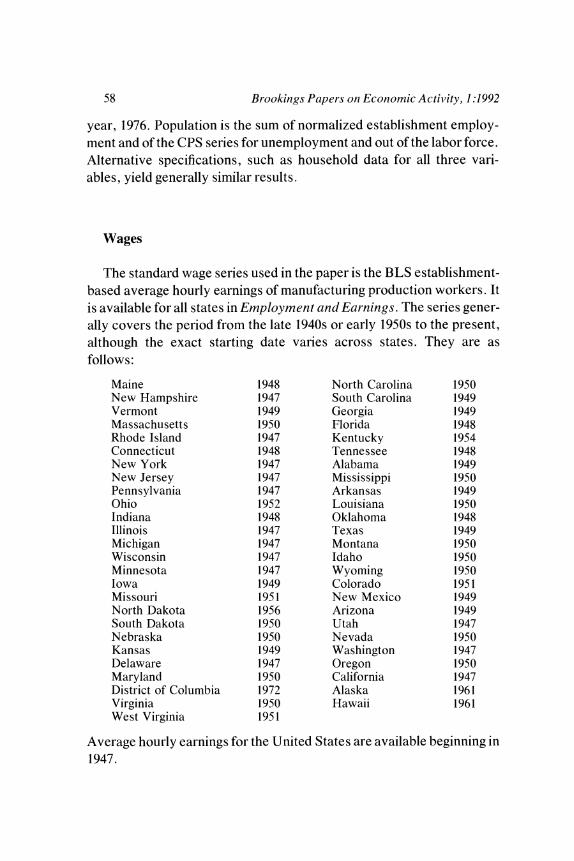
58 Brookings Papers on Economic Actiity, 1:1992
year, 1976. Population is the sum of normalized establishment employ- ment and of the CPS series for unemployment and out of the labor force. Alternative specifications, such as household data for all three vari- ables, yield generally similar results.
Wages
The standard wage series used in the paper is the BLS establishment- based average hourly earnings of manufacturing production workers. It is available for all states in Employment and Earnings. The series gener- ally covers the period from the late 1940s or early 1950s to the present, although the exact starting date varies across states. They are as follows:
Maine 1948 North Carolina 1950 New Hampshire 1947 South Carolina 1949 Vermont 1949 Georgia 1949 Massachusetts 1950 Florida 1948 Rhode Island 1947 Kentucky 1954 Connecticut 1948 Tennessee 1948 New York 1947 Alabama 1949 New Jersey 1947 Mississippi 1950 Pennsylvania 1947 Arkansas 1949 Ohio 1952 Louisiana 1950 Indiana 1948 Oklahoma 1948 Illinois 1947 Texas 1949 Michigan 1947 Montana 1950 Wisconsin 1947 Idaho 1950 Minnesota 1947 Wyoming 1950 Iowa 1949 Colorado 1951 Missouri 1951 New Mexico 1949 North Dakota 1956 Arizona 1949 South Dakota 1950 Utah 1947 Nebraska 1950 Nevada 1950 Kansas 1949 Washington 1947 Delaware 1947 Oregon 1950 Maryland 1950 California 1947 District of Columbia 1972 Alaska 1961 Virginia 1950 Hawaii 1961 West Virginia 1951
Average hourly earnings for the United States are available beginning in 1947.
Olivier Jean Blanchard and Lawrence F. Katz 59
The wage measure that controls for industry and worker characteris- tics was constructed annually from 1979 to 1989 from the CPS. Each month, the CPS collects wage information from one-quarter of its sam- ple. Using these wages, we estimated earnings equations each year for men and women separately. Log usually hourly wages were regressed on linear, quadratic, cubic, and quartic experience terms and dummy variables capturing an individual's education level, racial background, urban-rural residence, and full-time or part-time work status, as well as the occupation and industry in which the individual is employed. We then constructed the worker-characteristic-controlled wage for each year in each state as the average residual across all males and females in the state for that year. Results of the earnings function estimation are available upon request.
Per Capita Income
State per capita income is constructed using personal income from the Bureau of Economic Analysis Survey of Current Business for 1948- 90 (except for the District of Columbia, Alaska, and Hawaii series, which begin in 1958); and total resident population from the Census Bu- reau' s P-25 publication for 1948-90.
City House Prices
City house prices are median house prices of existing single family homes for 39 cities and the United States published in the National Asso- ciation of Realtors Home Sales Yearbook and taken from Poterba (1991). The data cover the period up to 1990; start dates vary across cit- ies. The cities and start dates are as follows:
Boston, MA 1969 Akron, OH 1980 Providence, RI 1979 Columbus, OH 1979 Hartford, CT 1980 Indianapolis, IN 1979 Albany, NY 1979 Chicago, IL 1969 New York, NY 1969 Detroit, MI 1969 Rochester, NY 1979 Grand Rapids, MI 1980 Syracuse, NY 1980 Milwaukee, WI 1973 Philadelphia, PA 1969 Minneapolis, MN 1969
60 Brookings Papers on Economic Actiity, 1:1 992
Des Moines, IA 1980 Tulsa, OK 1980 Kansas City, MO 1979 El Paso, TX 1980 St. Louis, MO 1973 Houston, TX 1969 Baltimore, MD 1969 San Antonio, TX 1979 Washington, DC 1973 Albuquerque, NM 1980 Atlanta, GA 1969 Salt Lake City, UT 1979 Ft. Lauderdale, FL 1979 Los Angeles, CA 1969 Tampa, FL 1979 Riverside, CA 1979 Louisville, KY 1980 Sacramento, CA 1980 Memphis, TN 1979 San Diego, CA 1979 Nashville, TN 1980 San Francisco, CA 1969 Birmingham, AL 1979
City Consumer Prices
Consumer prices used in the paper are consumer price indexes for all urban consumers and all items. These data range from 1965 to 1988 for the following 23 cities:
Atlanta, GA Dallas, TX Miami, FL San Diego, CA Baltimore, MD Denver, CO Milwaukee, WI San Francisco, CA Boston, MA Detroit, MI Minneapolis, MN Seattle, WA Chicago, IL Houston, TX New York, NY St. Louis, MO Cincinnati, OH Kansas City, MO Philadelphia, PA Washington, DC Cleveland, OH Los Angeles, CA Pittsburgh, PA
Net Migration
Net migration figures are from Barro and Sala-i-Martin (1991). They are averages of annual net migration, divided by initial state population for the periods 1950-60, 1960-70, 1970-80, and 1980-87.
Defense Spending
The measure of defense spending used in the paper is the real value of military prime contract awards by state from Davis, Loungani, and Mahidhara (1991). The series is deflated using the 1982 GNP deflator and ranges from 1951 to 1988 in calendar years (except for Alaska and Hawaii, whose observations begin in 1960).

Olivier Jean Blanchard and Lawrence F. Katz 61
Mix Variable
The mix variable was constructed and given to us by Timothy Bartik along the lines of Bartik (1991). The variable measures the predicted em- ployment growth rate for each state in each year under the assumption that each of the state's two-digit industries had the same employment growth rate as the national average employment growth rate for that sector.
Comments and Discussion
Robert E. Hall: Olivier Blanchard and Lawrence Katz provide an ex- traordinarily careful and insightful investigation of labor-market dynam- ics at the level of the states of the United States. The paper reaches sur- prisingly strong conclusions about the predominance of migration over other forms of adjustment to changing economic fundamentals at the state level in the longer run. After seven years, they find, an increase in demand results entirely in an increase in employment, with no increase in labor force participation or decrease in unemployment. In the longer run, quantities, not prices, make the adjustment.
My first comment is that the longer run is pretty long. The responses at the state level are at considerably lower frequencies than the national business cycle. A state or regional cycle at roughly the five-year fre- quency is superimposed on the generally faster national cycle. Thus the best forecast of national unemployment three years from now is full em- ployment, but unemployment in any particular state would be forecast to be lower than now if conditions are worse in the state than the nation this year.
The economic model supported by the results is easy to describe. The supply of labor to any state is perfectly elastic in the longer run. Any shift in labor demand at the state level causes a movement along a hori- zontal labor supply schedule. In the theoretical model, equation 6 com- pels perfectly elastic long-run labor supply because labor supply keeps growing as long as there is any wage differential. However, the empirical work does not build in this assumption; it is a derived conclusion.
The core evidence on labor supply is summarized right at the begin- ning of the paper: large and persistent differences in employment growth occur across states. Figure 2 shows these differences dramatically. By
62
Olivier Jean Blanchard and Lawrence F. Katz 63
contrast, relative unemployment rates show only transitory departures from an underlying structure of relative rates dictated by employment mix. The annual mean reversion coefficients generally lie in the range from 20 percent to 40 percent. Individually, these are not significantly different from zero.
To complete the story, the authors should also investigate the persis- tence of changes in labor force participation. The only evidence on this point is later, in the fourth section ("Employment, Unemployment, and Participation"), where we find the simple statement that labor force par- ticipation in a state (relative to the national average), along with employ- ment growth and unemployment, "appear to be stationary." It would be useful to see a bit more of the evidence.
The conclusion favoring perfectly elastic long-run labor supply is in- evitable, given the behavior of the three variables. If employment in a state can change a great deal and tends to remain at the new level, but unemployment and labor force participation return to normal, then no other possible conclusion exists but that the population has changed to accommodate the higher employment.
The detailed study of this issue in the fourth section, based on a three- variable VAR, is useful confirmation of the proposition that unemploy- ment and labor force participation do not absorb state-level shocks in the longer run. In a sense, the VAR is unnecessary. It could show that even though there were persistent movements in unemployment and participation, those movements were exogenous and not associated with the persistent movements in employment. But in fact there are no persistent movements in unemployment and participation, so we never reach the question that the VAR could answer. The univariate proper- ties of the three variables dictate the findings of the VAR.
An important econometric shortcoming infects the methods used to reach the basic conclusion of the paper. The samples are extremely short by the standards of time-series econometrics. The VAR has only 13 observations and the univariate analysis of unemployment has only 19 observations. A dictum of time-series statistics holds that the persis- tence of a time-series is understated by estimation in short samples. The replication across states does nothing to relieve the downward bias, al- though it reduces the sampling error of the estimates. Samples as short as those used by Blanchard and Katz are strictly terra incognita within time-series econometrics.
64 Br ookings Paipers on Economic Activity, 1.:1992
Because a downward bias occurs in the estimates of the persistence of employment as well, I suspect that the stark difference between the high persistence of employment and the low persistence of unemploy- ment and participation at the state level will withstand corrections for small-sample bias. The question is then what to make of the finding, within the supply-demand framework. The authors argue aggressively that the finding that unemployment and participation do not track em- ployment in the longer run supports the perfectly-elastic-labor-supply view because the employment changes are the result exclusively of shifts of the demand schedule, without shifts of the supply schedule.
The authors always state this identification hypothesis in terms of the innovations in employment, which they interpret as shocks to demand, rather than supply. In their model, employment is the moving average of its own current and past innovations and of past innovations in the labor force and participation rate. The paper does not reveal the relative importance of the demand shock, on the one hand, and the lagged labor force and participation shocks, on the other hand. To the extent that most of the action comes from the demand shock, the authors actually are saying that the persistent, as well as the unexpected, movements in employment are caused by shifts in demand and not in supply. I found it useful to ponder the panels of figure 2 in thinking about this issue. The panel for the oil states is pretty convincing. Be sure to keep your eye on the different vertical scales of the graphs in figure 2. By far the biggest fact in the figure is the extreme growth of the Sun Belt states. The identi- fying hypothesis says that demand shifts in the national economy for products in which California and Florida have comparative advantages caused the extreme excess growth of the Sun Belt. It is essential to stress that the conditions that might affect labor supply-the favorable cli- mates of the Sun Belt states-are permanent and could not have a role in changes in employment, except for chronic differences in growth rates. One would have to assert a shift of preferences toward sunny states to get a supply shift.
I would accept Blanchard and Katz's conclusion that labor supply is highly elastic to a particular state in the longer run. I would add that la- bor demand is also highly elastic, as in the theoretical model in this pa- per. The state distribution of employment is then a matter of a fragile equilibrium: very small changes in either supply or demand cause large changes in employment in the longer run. The spatial distribution of em-
Olivier Jean Blanchard and Lawrence F. Katz 65
ployment is close to indeterminate. Because of increasing returns in the types of activities that occur in cities, large cities develop in natural ag- glomeration points. A significant part of the overall findings of this paper has to do with the explosive growth of huge modern metropolitan areas in Arizona, California, and Florida.
Running through the paper is a suggestion that the persistent effect of a demand shock tells us something about the strength of economic forces that counteract the shock. For example, the authors argue that most of the adjustment to an adverse shock of employment is through out-migration of labor, rather than through the in-migration or creation of jobs. At this point, the only evidence they have marshaled in favor of the proposition is the extreme persistence of the effects of what they consider demand shocks. They seem to assume that demand shifts are inherently one-time random-walk shifts, so that the effects a year later and after are the result of endogenous responses. But no basis exists for this implicit assumption. The demand shift itself could have any form of persistence. All that is observed in the data used in this paper and dis- played in the impulse response diagrams is the net effect of a possibly persistent demand change and the offsetting adjustment through wage changes.
Later in the paper, the authors support their view by showing that there is little feedback in their model through wages. If we accept all of their identifying assumptions, we must conclude that there is relatively little shock absorption by wages. Even in the short run, labor supply is effectively highly wage elastic, possibly because of wage rigidity.
The authors deserve congratulations for pulling together an impres- sive body of evidence on the joint behavior of employment, unemploy- ment, wages, and housing prices. By and large, the data support current ideas about the determinants of economic activity. States do not have natural levels of employment, dictated by a neoclassical long-run equi- librium with diminishing returns to crowding extra labor in a given state. Instead, agglomeration efficiencies are great enough to make the distri- bution of employment across states indeterminate. Temporary shocks leave permanent legacies.
Barry Eichengreen: Olivier Blanchard and Larry Katz have done a sig- nal service by helping to awaken the profession to the importance of re- gional economics. In the same sense that all politics is local, it might be
66 Br-ookings Papers on Economic Activity, 1:1992
said that all macroeconomics is regional. It is important to think harder than we traditionally have about the market area or region to which a particular macroeconomic analysis applies.
The appeal of the paper lies in the simple and intuitive story it tells. (I will introduce its elements in a different sequence than the authors.) Adjustments to regional labor demand shocks occur mainly through in- terregional migration. If labor demand falls in a depressed region such as Massachusetts, unemployment rises there. Workers emigrate to lower unemployment regions. During this transition, aggregate employment grows more slowly in depressed regions than in other regions. After sev- eral years-six to ten years, in the case of Massachusetts-the unem- ployment rate has returned to the national average. However, the level of employment is permanently lower in the depressed region and perma- nently higher elsewhere. (For the rest of this commentary, I will refer to Massachusetts as a shorthand for depressed regions.)
This story as I have told it has two obvious limitations, one of which the authors deal with more satisfactorily than the other. The first is wage adjustment. Implicit in the summary of the previous paragraph is the as- sumption that wages in Massachusetts do not decline sufficiently to ra- tion all of the unemployed back into work. Blanchard and Katz show that some decline of relative wages occurs in Massachusetts, but that it is slow and does little to shift the adjustment burden away from migra- tion. Just why wage relativities across regions should be so inflexible as to permit regional unemployment rates to diverge for six to ten years is unclear. I will return to this question in another context.
The second limitation of this story is that it is not clear, as I have de- scribed it, why employment growth rates (as opposed to levels) should continue to differ across states or regions for at least four decades, and perhaps longer, as figure 1 in the paper suggests they do. After six years or so, migration should be complete and unemployment in Massachu- setts should have returned to the national average. The labor force will have contracted permanently in Massachusetts (relative to its underly- ing trend) and expanded permanently elsewhere. Thereafter, all states should grow at the same rate as before and, in the absence of additional complications, at the same rate as one another. Yet figure 1 shows that employment persistently grows at different rates in different states.
Blanchard and Katz explain this finding by adding, somewhat arbi- trarily, region-specific effects to their migration and labor demand equa-
Olivier Jean Blanchard and Lawrence F. Katz 67
tions. Thus they replicate the persistent employment growth differen- tials across regions found in the data by assuming particular processes for the forcing variables, not through the intrinsic dynamics of their model. In a reference ideally designed to disarm their discussants, they justify the extra term in the migration equation by appealing to the at- tractiveness of the California lifestyle. They justify the additional term in the labor demand equation by asserting that the supply and demand curves for the different goods in which different regions specialize per- sistently shift outward at different rates.
Let me suggest two additional sources of long-term employment growth differentials across regions. One is the settlement patterns of im- migrants. Immigrants from Asia or Mexico are more likely to arrive in California than, say, Iowa, and once there, to settle, because prior immi- grants who have not yet moved away from the port of entry provide a natural network through which social and economic information can be transmitted. One might argue that, in response to immigration from Asia to California, wages in California should decline and unemployment there should rise, discouraging in-migration from other states and main- taining the equality of long-term employment growth rates between them. Alternatively, native and immigrant workers may be comple- ments rather than substitutes, in which case these implications do not follow. 1 Either way, the neglect of immigration from abroad is one of the more serious limitations of Blanchard and Katz's paper and a prominent omission from their research agenda.
A second category of explanation would build on the literature on hysteresis in unemployment. There has been a fair amount of work at- tempting to test-not very successfully, one must admit-reasons why a one-time shock to labor demand might have permanent effects on the level of unemployment. Some of these arguments might be adapted to explain persistent differences across regions in the growth of employ- ment. One is struck by the absence of such issues from a paper that has as one of its coauthors the godfather of much of the hysteresis literature. An advantage of pursuing this tack is that it would provide an opening to the literature in regional economics, much of which emphasizes more than the authors do the absence of self-correcting responses to regional employment decline.2
1. So Keynes argues for the United States. See Thomas (1958, p. 382). 2. See Heim (1992).
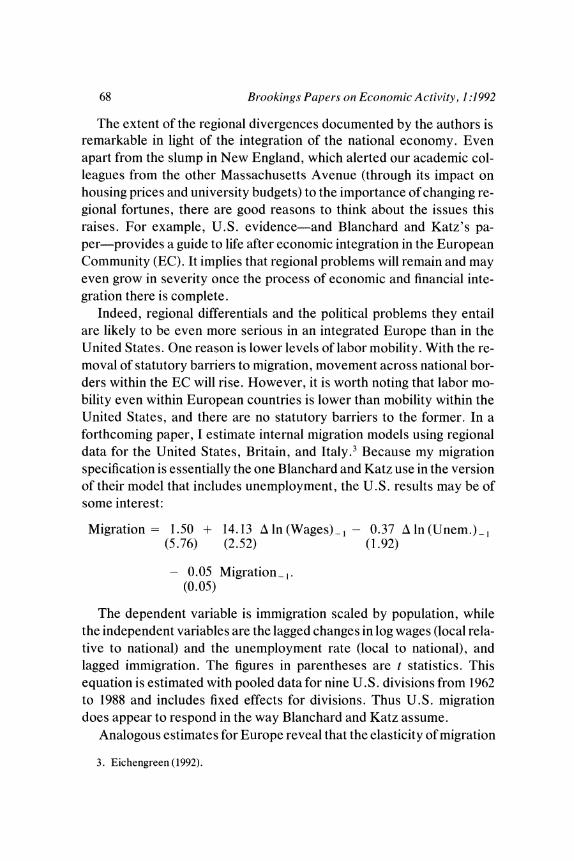
68 Brookings Papers on Economic Activity, 1:1992
The extent of the regional divergences documented by the authors is remarkable in light of the integration of the national economy. Even apart from the slump in New England, which alerted our academic col- leagues from the other Massachusetts Avenue (through its impact on housing prices and university budgets) to the importance of changing re- gional fortunes, there are good reasons to think about the issues this raises. For example, U.S. evidence-and Blanchard and Katz's pa- per-provides a guide to life after economic integration in the European Community (EC). It implies that regional problems will remain and may even grow in severity once the process of economic and financial inte- gration there is complete.
Indeed, regional differentials and the political problems they entail are likely to be even more serious in an integrated Europe than in the United States. One reason is lower levels of labor mobility. With the re- moval of statutory barriers to migration, movement across national bor- ders within the EC will rise. However, it is worth noting that labor mo- bility even within European countries is lower than mobility within the United States, and there are no statutory barriers to the former. In a forthcoming paper, I estimate internal migration models using regional data for the United States, Britain, and Italy.3 Because my migration specification is essentially the one Blanchard and Katz use in the version of their model that includes unemployment, the U.S. results may be of some interest:
Migration = 1.50 + 14.13 A ln (Wages)1 - 0.37 Iln (Unem.)_ (5.76) (2.52) (1.92)
- 0.05 Migration-,. (0.05)
The dependent variable is immigration scaled by population, while the independent variables are the lagged changes in log wages (local rela- tive to national) and the unemployment rate (local to national), and lagged immigration. The figures in parentheses are t statistics. This equation is estimated with pooled data for nine U.S. divisions from 1962 to 1988 and includes fixed effects for divisions. Thus U.S. migration does appear to respond in the way Blanchard and Katz assume.
Analogous estimates for Europe reveal that the elasticity of migration
3. Eichengreen (1992).
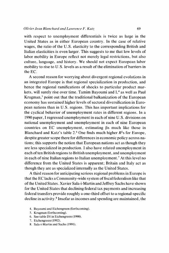
Olivier Jean Blanchard and Lawrence F. Katz 69
with respect to unemployment differentials is twice as large in the United States as in either European country. In the case of relative wages, the ratio of the U.S. elasticity to the corresponding British and Italian elasticities is even larger. This suggests to me that low levels of labor mobility in Europe reflect not merely legal restrictions, but also culture, language, and history. We should not expect European labor mobility to rise to U.S. levels as a result of the elimination of barriers in the EC.
A second reason for worrying about divergent regional evolutions in an integrated Europe is that regional specialization in production, and hence the regional ramifications of shocks to particular product mar- kets, will surely rise over time. Tamim Bayoumi and I,' as well as Paul Krugman,5 point out that the traditional balkanization of the European economy has sustained higher levels of sectoral diversification in Euro- pean nations than in U.S. regions. This has important implications for the cyclical behavior of unemployment rates in different regions. In a 1990 paper, I regressed unemployment in each of nine U.S. divisions on national unemployment and unemployment in each of nine European countries on EC unemployment, estimating Ps much like those in Blanchard and Katz's table 2.6 One finds much higher R2s for Europe, despite greater scope there for differences in economic policy across na- tions; this supports the notion that European nations act as though they are less specialized in production. I also have related unemployment in each of ten British regions to British unemployment, and unemployment in each of nine Italian regions to Italian unemployment.7 At this level no difference from the United States is apparent; Britain and Italy act as though they are as specialized internally as the United States.
A third reason for anticipating serious regional problems in Europe is that the EC lacks a Community-wide system of fiscal federalism like that of the United States. Xavier Sala-i-Martin and Jeffrey Sachs have shown for the United States that declining federal tax payments and increasing federal transfers provide roughly a one-third offset to a regional-specific decline in activity.8 Insofar as incomes and spending are maintained, the
4. Bayoumi and Eichengreen (forthcoming). 5. Krugman (forthcoming). 6. See table DI in Eichengreen (1990). 7. Eichengreen (1992). 8. Sala-i-Martin and Sachs (1991).
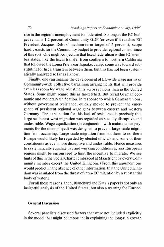
70 Brookings Papers on Economic Activity, 1:1992
rise in the region's unemployment is moderated. So long as the EC bud- get remains 1.2 percent of Community GDP (or even if it reaches EC President Jacques Delors' medium-term target of 2 percent), scope hardly exists for the Community budget to provide regional coinsurance of this sort. One might conjecture that fiscal federalism within EC mem- ber states, like the fiscal transfer from southern to northern California that followed the Loma Prieta earthquake, can go some way toward sub- stituting for fiscal transfers between them, but this has not been system- atically analyzed so far as I know.
Finally, one can imagine the development of EC-wide wage norms or Community-wide collective bargaining arrangements that will provide even less room for wage adjustments across regions than in the United States. Some might regard this as far-fetched. But recall German eco- nomic and monetary unification, in response to which German unions, without government resistance, quickly moved to prevent the emer- gence of persistent regional wage gaps between eastern and western Germany. The explanation for this lack of resistance is precisely that large-scale east-west migration was regarded as socially disruptive and undesirable. Wage equalization (in conjunction with maintenance pay- ments for the unemployed) was designed to prevent large-scale migra- tion from occurring. Large-scale migration from southern to northern Europe would likely be regarded by elected officials and some of their constituents as even more disruptive and undesirable. Hence measures to systematically equalize pay and working conditions across European regions might be encouraged to limit the incentive to migrate. We see hints of this in the Social Charter embraced at Maastricht by every Com- munity member except the United Kingdom. (From this argument one would predict, in the absence of other information, that the United King- dom was insulated from the threat of intra-EC migration by a substantial body of water.)
For all these reasons, then, Blanchard and Katz's paper is not only an insightful analysis of the United States, but also a warning for Europe.
General Discussion
Several panelists discussed factors that were not included explicitly in the model that might be important in explaining the long-run growth
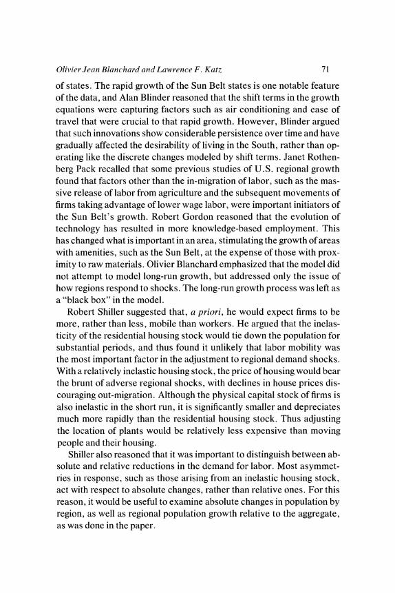
Olivier Jean Blanchard and Lawrence F. Katz 71
of states. The rapid growth of the Sun Belt states is one notable feature of the data, and Alan Blinder reasoned that the shift terms in the growth equations were capturing factors such as air conditioning and ease of travel that were crucial to that rapid growth. However, Blinder argued that such innovations show considerable persistence over time and have gradually affected the desirability of living in the South, rather than op- erating like the discrete changes modeled by shift terms. Janet Rothen- berg Pack recalled that some previous studies of U.S. regional growth found that factors other than the in-migration of labor, such as the mas- sive release of labor from agriculture and the subsequent movements of firms taking advantage of lower wage labor, were important initiators of the Sun Belt's growth. Robert Gordon reasoned that the evolution of technology has resulted in more knowledge-based employment. This has changed what is important in an area, stimulating the growth of areas with amenities, such as the Sun Belt, at the expense of those with prox- imity to raw materials. Olivier Blanchard emphasized that the model did not attempt to model long-run growth, but addressed only the issue of how regions respond to shocks. The long-run growth process was left as a "black box" in the model.
Robert Shiller suggested that, a priori, he would expect firms to be more, rather than less, mobile than workers. He argued that the inelas- ticity of the residential housing stock would tie down the population for substantial periods, and thus found it unlikely that labor mobility was the most important factor in the adjustment to regional demand shocks. With a relatively inelastic housing stock, the price of housing would bear the brunt of adverse regional shocks, with declines in house prices dis- couraging out-migration. Although the physical capital stock of firms is also inelastic in the short run, it is significantly smaller and depreciates much more rapidly than the residential housing stock. Thus adjusting the location of plants would be relatively less expensive than moving people and their housing.
Shiller also reasoned that it was important to distinguish between ab- solute and relative reductions in the demand for labor. Most asymmet- ries in response, such as those arising from an inelastic housing stock, act with respect to absolute changes, rather than relative ones. For this reason, it would be useful to examine absolute changes in population by region, as well as regional population growth relative to the aggregate, as was done in the paper.
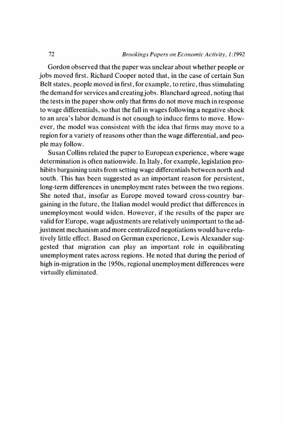
72 Brookings Papers on Economic Activity, 1:1992
Gordon observed that the paper was unclear about whether people or jobs moved first. Richard Cooper noted that, in the case of certain Sun Belt states, people moved in first, for example, to retire, thus stimulating the demand for services and creatingjobs. Blanchard agreed, noting that the tests in the paper show only that firms do not move much in response to wage differentials, so that the fall in wages following a negative shock to an area's labor demand is not enough to induce firms to move. How- ever, the model was consistent with the idea that firms may move to a region for a variety of reasons other than the wage differential, and peo- ple may follow.
Susan Collins related the paper to European experience, where wage determination is often nationwide. In Italy, for example, legislation pro- hibits bargaining units from setting wage differentials between north and south. This has been suggested as an important reason for persistent, long-term differences in unemployment rates between the two regions. She noted that, insofar as Europe moved toward cross-country bar- gaining in the future, the Italian model would predict that differences in unemployment would widen. However, if the results of the paper are valid for Europe, wage adjustments are relatively unimportant to the ad- justment mechanism and more centralized negotiations would have rela- tively little effect. Based on German experience, Lewis Alexander sug- gested that migration can play an important role in equilibrating unemployment rates across regions. He noted that during the period of high in-migration in the 1950s, regional unemployment differences were virtually eliminated.
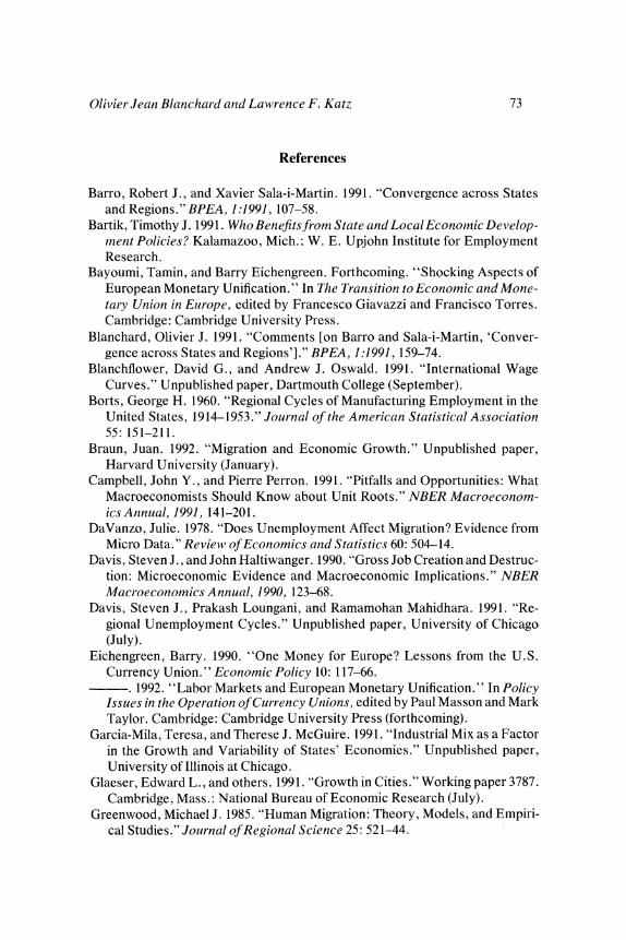
Olivier Jean Blanchar-d anid Lawrence F. Katz 73
References
Barro, Robert J., and Xavier Sala-i-Martin. 1991. "Convergence across States and Regions." BPEA, 1:1991, 107-58.
Bartik, Timothy J. 1991. Who Benefitsfrom State and Local Economic Develop- ment Policies? Kalamazoo, Mich.: W. E. Upjohn Institute for Employment Research.
Bayoumi, Tamin, and Barry Eichengreen. Forthcoming. "Shocking Aspects of European Monetary Unification." In The Transition to Economic and Mone- taly Union in Eirope, edited by Francesco Giavazzi and Francisco Torres. Cambridge: Cambridge University Press.
Blanchard, Olivier J. 1991. "Comments [on Barro and Sala-i-Martin, 'Conver- gence across States and Regions']." BPEA, 1:1991, 159-74.
Blanchflower, David G., and Andrew J. Oswald. 1991. "International Wage Curves." Unpublished paper, Dartmouth College (September).
Borts, George H. 1960. "Regional Cycles of Manufacturing Employment in the United States, 1914-1953." Journal of the American Statistical Association 55: 151-211.
Braun, Juan. 1992. "Migration and Economic Growth." Unpublished paper, Harvard University (January).
Campbell, John Y., and Pierre Perron. 1991. "Pitfalls and Opportunities: What Macroeconomists Should Know about Unit Roots." NBER Macroeconom- ics Annual, 1991, 141-201.
DaVanzo, Julie. 1978. "Does Unemployment Affect Migration? Evidence from Micro Data." Review of Economics and Statistics 60: 504-14.
Davis, Steven J., and John Haltiwanger. 1990. "Gross Job Creation and Destruc- tion: Microeconomic Evidence and Macroeconomic Implications." NBER Macroeconomics Annual, 1990, 123-68.
Davis, Steven J., Prakash Loungani, and Ramamohan Mahidhara. 1991. "Re- gional Unemployment Cycles." Unpublished paper, University of Chicago (July).
Eichengreen, Barry. 1990. "One Money for Europe? Lessons from the U.S. Currency Union." Economic Policy 10: 117-66.
. 1992. "Labor Markets and European Monetary Unification." In Policy Issues in the Operation of Currency Unions, edited by Paul Masson and Mark Taylor. Cambridge: Cambridge University Press (forthcoming).
Garcia-Mila, Teresa, and Therese J. McGuire. 1991. "Industrial Mix as a Factor in the Growth and Variability of States' Economies." Unpublished paper, University of Illinois at Chicago.
Glaeser, Edward L., and others. 1991. "Growth in Cities." Working paper 3787. Cambridge, Mass.: National Bureau of Economic Research (July).
Greenwood, Michael J. 1985. "Human Migration: Theory, Models, and Empiri- cal Studies." Jolurnal ofRegional Science 25: 521-44.
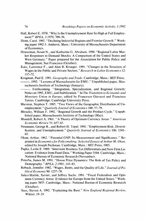
74 Brookin2s PaDers on Economic Activity, 1:1992
Hall, Robert E. 1970. "Why Is the Unemployment Rate So High at Full Employ- ment?" BPEA, 3:1970, 709-56.
Heim, Carol. 1992. "Declining Industrial Regions and Frontier Growth." Work- ing paper 1992-5. Amherst, Mass.: University of Massachusetts Department of Economics.
Houseman, Susan N., and Katharine G. Abraham. 1990. "Regional Labor Mar- ket Responses to Demand Shocks: A Comparison of the United States and West Germany." Paper prepared for the Association for Public Policy and Management, San Francisco (October).
Katz, Lawrence F., and Alan B. Krueger. 1991. "Changes in the Structure of Wages in the Public and Private Sectors." Research in Labor Economics 12: 137-72.
Krugman, Paul E. 1991. Geography and Trade. Cambridge, Mass.: MIT Press. . 1992. "Lessons of Massachusetts for EMU." Unpublished paper, Mas-
sachusetts Institute of Technology (January). . Forthcoming. "Integration, Specialization, and Regional Growth:
Notes on 1992, EMU, and Stabilization." In The Transition to Economic and Monetary Union in Europe, edited by Francesco Giavazzi and Francisco Torres. Cambridge: Cambridge University Press.
Marston, Stephen T. 1985. "Two Views of the Geographic Distribution of Un- employment." Quarterly Journal of Economics 100: 57-79.
Miracky, William F. 1992. "Regional Growth and the Product Cycle." Unpub- lished paper, Massachusetts Institute of Technology (May).
Mundell, Robert A. 1961. "A Theory of Optimum Currency Areas." American Economic Review 51: 657-65.
Neumann, George R., and Robert H. Topel. 1991. "Employment Risk, Diversi- fication, and Unemployment." Quarterly Jour-nal of Economics 106: 1341- 65.
Okun, Arthur. 1962. "Potential GNP: Its Measurement and Significance." Re- printed in Economics for Policymaking: Selected Essays of Arthlur M. Oklun, edited by Joseph Pechman. Cambridge, Mass.: MIT Press, 1983.
Papke, Leslie E. 1989. "Interstate Business Tax Differentials and New Firm Lo- cation: Evidence from Panel Data. " Working Paper 3184. Cambridge, Mass.: National Bureau of Economic Research (November).
Poterba, James M. 1991. "House Price Dynamics: The Role of Tax Policy and Demography." BPEA, 2:1991, 143-83.
Roback, Jennifer. 1982. "Wages, Rents, and the Quality of Life." Journal of Po- litical Economy 90: 1257-78.
Sala-i-Martin, Xavier, and Jeffrey Sachs. 1991. "Fiscal Federalism and Opti- mum Currency Areas: Evidence for Europe from the United States." Work- ing paper 3855. Cambridge, Mass.: National Bureau of Economic Research (October).
Sass, Steven A. 1992. "Explaining the Bust." New England Regional Review, Winter, 19-24.
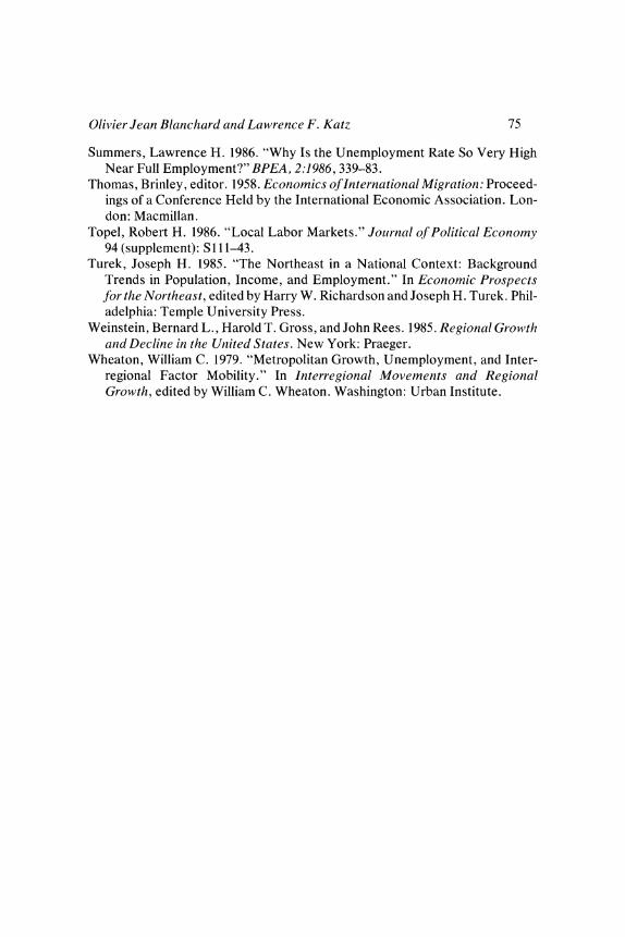
Olivier Jean Blanchard and Lawrence F. Katz 75
Summers, Lawrence H. 1986. "Why Is the Unemployment Rate So Very High Near Full Employment?" BPEA, 2:1986, 339-83.
Thomas, Brinley, editor. 1958. Economics of International Migration: Proceed- ings of a Conference Held by the International Economic Association. Lon- don: Macmillan.
Topel, Robert H. 1986. "Local Labor Markets." Joiurnal of Political Economy 94 (supplement): S 1 1-43.
Turek, Joseph H. 1985. "The Northeast in a National Context: Background Trends in Population, Income, and Employment." In Economic Prospects for the Northeast, edited by Harry W. Richardson and Joseph H. Turek. Phil- adelphia: Temple University Press.
Weinstein, Bernard L., Harold T. Gross, and John Rees. 1985. Regional Growth and Decline in the United States. New York: Praeger.
Wheaton, William C. 1979. "Metropolitan Growth, Unemployment, and Inter- regional Factor Mobility." In Interregional Movements and Regional Growth, edited by William C. Wheaton. Washington: Urban Institute.