1

Working Paper No. 03-07

Regional employment growth and the persistence of regional unemployment disparities

William Mitchell and Ellen Carlson

June 2003

Centre of Full Employment and Equity The University of Newcastle, Callaghan NSW 2308, Australia

Home Page: http://e1.newcastle.edu.au/coffee Email: coffee@newcastle.edu.au

2

1. Introduction A contested issue in regional economic debate concerns the relative importance of regional-specific versus macroeconomic factors in determining regional employment outcomes. The theoretical impasse is also evident in regional development policy (Rissman, 1999). Keynesian macroeconomics typically argues that regional employment variations are caused by the impact of the national business cycle on growth rates across industries, which reflect changes in aggregate factors, such as fiscal and monetary policy settings, business and consumer confidence and productivity trends. Thus, the cyclical sensitivity of regional outcomes reflects the impact of common aggregate shocks and the specific regional industry mix. Regions dominated by goods-production allegedly lose employment share in recessions relative to service-providing regions. The solution is for aggregate policy to maintain strong growth with industry policy attenuating structural shifts.

The current Australian Government has pursued a different interpretation of the “macro” view and has eschewed both stimulatory macro policy and specific regional policy. Its low-inflation policy with fiscal restraint is designed to create a macro environment within which economic growth will flourish. Supplementary microeconomic reforms of the labour market and the welfare system aim to provide market incentives to promote individual participation in economic activity. Rather than introduce regionally-targetted policies, this strategy places faith in market forces to redress the regional problems - through labour mobility away from and firm relocation into areas of low labour utilisation response to falling wages and improved local labour skills.

While the national economy has demonstrated relatively robust output growth over the 1990s, it is clear that regional disparities in unemployment persist. The tight macro policy has sustained high unemployment and mobility patterns and relative wage movements have not promoted regional convergence (Martin, 1997; Debelle and Vickery, 1999). Disparities in regional incomes and employment are persistent and in many cases increasing (ALGA, 2002). For such reasons, the “macro” view (irrespective of the guise it takes) is now under challenge.

There is growing anecdotal evidence that regional development agencies are adopting a paradigm that has been termed new regionalism, which emerged in the mid-1980s and was inspired by case studies documenting economic successes in regions such as Silicon Valley and Baden Württemberg. Scott and Storper (1989) posited that regions had displaced nation states as sites of successful economic organisation. The upshot is that there is now an emphasis on localised institutions and collaborations. The status of macroeconomic policy is now considered peripheral to the growth potential of any particular region (Castells and Hall, 1994; Cooke and Morgan, 1998). Despite the growing popularity of new regionalism, the claim that the region offers a convincing theoretical explanation of recent and future economic development is under-researched and has weak empirical underpinnings. There is little known about how the national economy interacts with the regions. Further, no empirical evidence exists to verify assumptions of, first, the emergence of capitalism centred on spatialised, autonomous economies, and, second, a hollowed out, macro-weakened nation state (Lovering, 1999; Markusen, 1996).

In this paper we seek to develop an understanding of the linkages between regions with respect to employment growth and to determine the extent to which national

3

trends dominate location-specific dynamics. The empirical analysis of the business cycle impact on regions typically focuses on co-movements in employment or output across industries, which may obscure the co-movements across regions. To fully understand regional employment growth, the co-movements across regional economies also have to be studied. There is very little research on this issue. Regional research in Australia has also concentrated on state-level analysis, which is insufficient, given the significant intra-state disparity of labour markets. For example, Dixon and Shepherd (2001) study trends and cycles in State and Territory unemployment rates to test whether region-specific shocks dominated national factors. If national factors dominate then policies designed to reduce regional unemployment rates would be indistinguishable from equivalent national policies. They find that regional unemployment rates exhibit independent paths. Conversely, Debelle and Vickery (1999) conclude that national factors dominated movements in state unemployment rates. Dixon and Shepherd (2001), however, outline several statistical problems with their approach.

Clark (1998) quantified the roles of national, regional, and industry-specific shocks on U.S. regional employment growth (also Altonji and Ham, 1990; Blanchard and Katz, 1992). He found that 40 per cent of any regional cyclical innovation reflected region-specific factors although he was unable to estimate the underlying causes of the regional shocks. Rissman (1999) also found that both national and local shocks were important influences on regional employment growth. She found that regionally-specific shocks did not impact uniformly on employment growth across regions.

The paper is laid out as follows. Section 2 introduces some data and definitional issues. Section 3 provides motivation for the research by examining regional unemployment disparities and tests whether the unemployment ranking is inversely related to a region’s employment growth rate. Section 4 presents a detailed analysis of regional employment growth in terms of national industry trends and location-specific variation. Regression analysis is used and it is concluded that regional employment dynamics are the result of complex interactions between variations in the national business cycle and regionally-specific variations. There is also considerable disparity between the regions. Section 5 reinforces this conclusion with a shift-share analysis which decomposes regional employment growth into national industry effects and location-specific effects. Both are found to be important. Section 6 uses contingency table analysis to test the proposition that regional employment growth cycles are closely linked. The results indicate that there are clusters of related regions with several other regions exhibiting disconnected outcomes. Concluding remarks follow.

2. Data issues The typical unit of analysis for Australian regional studies, particularly in cross-national studies, has been the State/Territory (see Dixon and Shepherd, 2001). This is due to deficiencies in the available data. For example, it is difficult to obtain data for consistently defined regions at a lower level of aggregation. More detailed regional labour force data for Major Statistical Regions (MSRs) was first collected in 1986 through the Australian Labour Force Survey. There are currently 64 such regions in Australia. In this paper, the higher aggregation of capital city and rest of State is used with the ACT and NT being treated as complete regions. The use of the data at this level of aggregation reflects an attempt to refine our methodology, which will then be applied at the more disaggregated MSR level for all States/Territories in further

4

research. It should also be noted that data for capital city/rest of state are available from 1978, whereas the more disaggregated data are available only from 1986.

In this paper, regional employment growth (annualised) is defined as:

(1) 4100*log( / )it it ite E E −=

where Eit is the level of employment at time t in the ith region.

Similarly, national employment growth (annualised) is defined as:

(2) 4100*log( / )t t te E E −=

where Et is the total national employment level at time t.

Net regional employment growth is the difference between regional employment growth and national employment growth:

(3) netit it te e e= −

The net employment growth rate for each region thus indicates the changing share that each region has in total national employment.

The net unemployment rate is similarly defined as the difference between the regional unemployment rate (URi) and the national rate (UR):

(4) it it tur UR UR= −

Positive values indicate that the regional unemployment rate is below the national rate while for negative values the regional unemployment rate is above the national rate.

3. Regional distribution of unemployment

3.1 Regional unemployment rankings Dixon and Shepherd (2001) examine quarterly unemployment rates for the six Australian states and two territories from 1978:Q2 to 1999:Q1 and find no evidence of common trends between regions but do identify common cycles among the larger states with TAS and the Territories appearing to be disconnected. Their results suggest that there is no tendency towards convergence in “regional” unemployment rates even though, in the main, they are all influenced by broader cyclical forces. This contrasts with Debelle and Vickrey (1999: 262) who say there is “evidence of permanent (or at least very persistent) differences between state unemployment rates” and that state unemployment rates “are largely explained by national (aggregate) factors rather than region-specific factors” (Dixon and Shepherd, 2001: 258). However, both studies use the states/territories aggregation to depict a region. In this paper, we take the analysis to the next level of disaggregation as outlined in Section 2.

In Tables 1 and 2 summary statistics for the ranked unemployment rates (lowest to highest) are presented. Data are shown for the entire period 1978 to 2003 and for sub-periods of 1983:2 to 1990:3 and 1991:4 to 2003:1 (the sub-periods correspond to the dated business cycles identified in Mitchell, 2001). The sub-periods are used to highlight any differences in performance between the two recessions (1982 and 1991) and the growth period following the 1990s recession. The ranked unemployment rates are accompanied by the annual change in employment growth for each region for comparison. Employment growth is examined in detail in Section 4.

5

Over the entire period, the highest mean unemployment rates were in TAS, the regional areas of NSW and QLD and in Adelaide. The NT and the ACT had the lowest mean unemployment rates, followed by regional WA, Sydney, VIC, Melbourne and NSW.

Table 1 Regional unemployment rates and employment growth rates

1978:1-2003:1 1983:2-1990:3 1991:4-2003:1

UR %E UR %E UR %E

NT 6.06 3.21 NT 5.31 3.70 ACT 6.19 1.49

ACT 6.40 2.43 VIC_C 6.30 2.71 NT 6.30 2.23

WA_R 6.51 2.16 WA_R 6.55 2.79 NSW_C 6.82 1.77

NSW_C 6.74 1.67 NSW_C 7.24 2.43 WA_R 6.95 1.97

VIC_C 7.38 1.60 ACT 7.28 4.69 WA_C 7.95 2.51

AUS 7.70 1.83 VIC_R 7.37 2.81 AUS 8.12 1.71

SA_R 7.84 0.64 AUS 7.77 2.80 SA_R 8.28 0.27

VIC_R 7.90 1.25 QLD_C 8.40 3.31 QLD_C 8.43 2.92

QLD_C 8.08 2.84 SA_R 8.42 1.39 VIC_C 8.50 1.72

WA_C 8.14 2.62 WA_C 8.47 3.69 VIC_R 9.04 0.88

QLD_R 8.91 2.93 SA_C 8.83 2.45 QLD_R 9.38 2.46

TAS_C 9.11 0.76 TAS_C 8.94 2.58 SA_C 9.63 0.81

SA_C 9.17 1.03 QLD_R 9.42 4.14 NSW_R 9.69 1.05

NSW_R 9.28 1.48 TAS_R 9.75 2.44 TAS_C 9.89 0.35

TAS_R 9.64 0.73 NSW_R 10.04 2.04 TAS_R 10.65 -0.15 Note: UR is the region’s unemployment rate in percent and %E is the region’s annual employment growth rate defined in Section 2. _C refers to the metropolitan region, while _R is the balance of the State. AUS is Australia. The UR’s are ranked from lowest to highest.

When the data are examined for the two separate periods we see that, in general, the areas that were below the Australian average over the whole period were also below it in each of the sub-periods. In all periods, the bottom positions are occupied by TAS, regional NSW, regional QLD and Adelaide. In the period between the 1980s and 1990s recession (middle columns), the Australian unemployment rate was similar to that for the period as a whole. Of the metropolitan regions, only Sydney and Melbourne experienced below average unemployment in that period. In the 1990s growth phase, the fortunes of Perth and Melbourne are reversed. The position of VIC is striking. Through the whole period and between the two recessions, VIC as a whole (not shown) and Melbourne performed better than the national average. Since the 1991 recession however, Melbourne (unemployment from 6.30 per cent to 8.50 per cent) and regional VIC (unemployment from 7.37 per cent between recessions to 9.04 per cent after) has performed poorly. The 1991 recession had a very serious and prolonged negative impact on VIC relative to other regions.

In Table 2, the dispersion of these unemployment rates (measured by the coefficient of variation) is shown. When examining the two separate periods (Columns 2 and 3), the position of each column relative to position in the unemployment rate rankings, is almost inversed. That is, the areas which had the highest unemployment rates tend

6

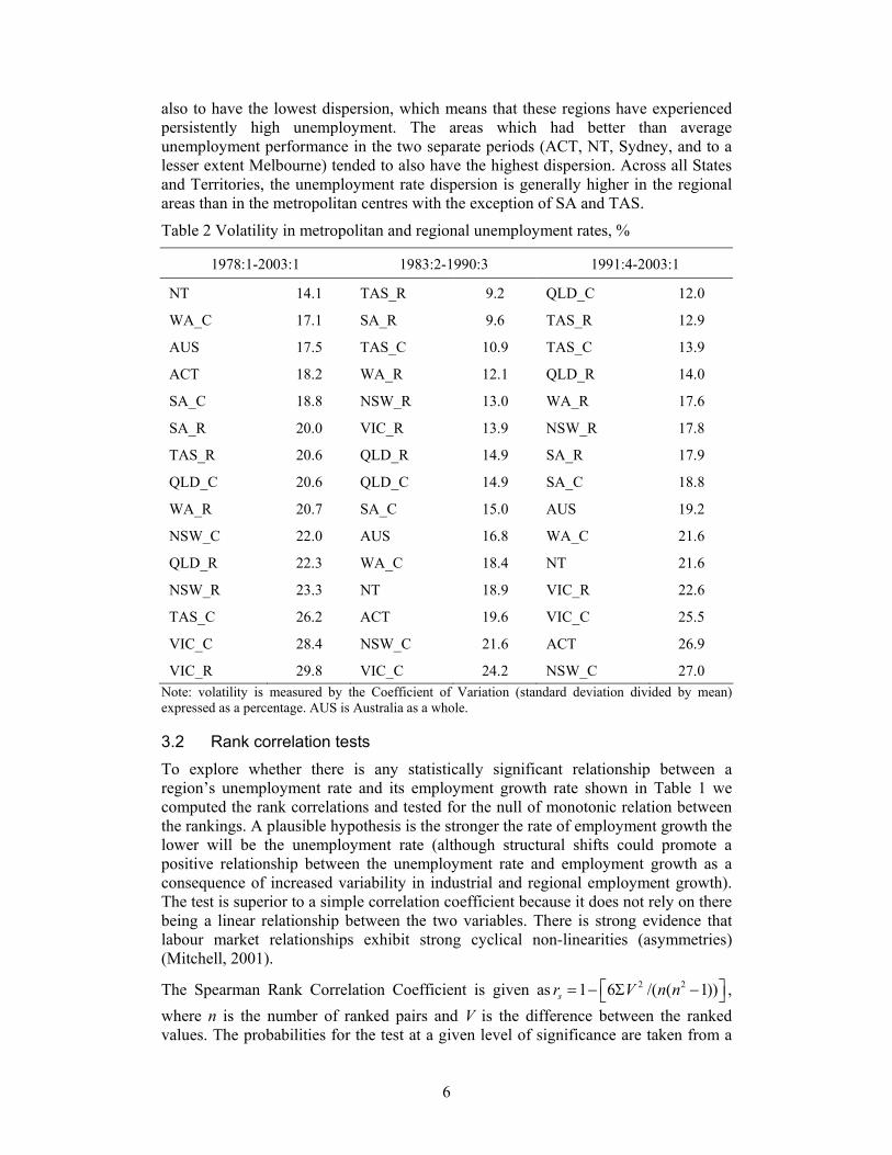
also to have the lowest dispersion, which means that these regions have experienced persistently high unemployment. The areas which had better than average unemployment performance in the two separate periods (ACT, NT, Sydney, and to a lesser extent Melbourne) tended to also have the highest dispersion. Across all States and Territories, the unemployment rate dispersion is generally higher in the regional areas than in the metropolitan centres with the exception of SA and TAS.

Table 2 Volatility in metropolitan and regional unemployment rates, %

1978:1-2003:1 1983:2-1990:3 1991:4-2003:1

NT 14.1 TAS_R 9.2 QLD_C 12.0

WA_C 17.1 SA_R 9.6 TAS_R 12.9

AUS 17.5 TAS_C 10.9 TAS_C 13.9

ACT 18.2 WA_R 12.1 QLD_R 14.0

SA_C 18.8 NSW_R 13.0 WA_R 17.6

SA_R 20.0 VIC_R 13.9 NSW_R 17.8

TAS_R 20.6 QLD_R 14.9 SA_R 17.9

QLD_C 20.6 QLD_C 14.9 SA_C 18.8

WA_R 20.7 SA_C 15.0 AUS 19.2

NSW_C 22.0 AUS 16.8 WA_C 21.6

QLD_R 22.3 WA_C 18.4 NT 21.6

NSW_R 23.3 NT 18.9 VIC_R 22.6

TAS_C 26.2 ACT 19.6 VIC_C 25.5

VIC_C 28.4 NSW_C 21.6 ACT 26.9

VIC_R 29.8 VIC_C 24.2 NSW_C 27.0 Note: volatility is measured by the Coefficient of Variation (standard deviation divided by mean) expressed as a percentage. AUS is Australia as a whole.

3.2 Rank correlation tests To explore whether there is any statistically significant relationship between a region’s unemployment rate and its employment growth rate shown in Table 1 we computed the rank correlations and tested for the null of monotonic relation between the rankings. A plausible hypothesis is the stronger the rate of employment growth the lower will be the unemployment rate (although structural shifts could promote a positive relationship between the unemployment rate and employment growth as a consequence of increased variability in industrial and regional employment growth). The test is superior to a simple correlation coefficient because it does not rely on there being a linear relationship between the two variables. There is strong evidence that labour market relationships exhibit strong cyclical non-linearities (asymmetries) (Mitchell, 2001).

The Spearman Rank Correlation Coefficient is given as 2 21 6 /( ( 1))sr V n n = − Σ − , where n is the number of ranked pairs and V is the difference between the ranked values. The probabilities for the test at a given level of significance are taken from a

7

(Olds, 1938). In our case, for n = 15, at the 5 per cent level for a one-sided test (given our a priori conjecture of a negative relationship), we reject the null ρ = 0 in favour of

0ρ ≠ if the test statistic, rs > 0.411.

We conducted the test on rankings (unemployment ranked from low to high and employment growth from high to low) for three periods: (a) the full sample, 1978:1 to 2003:1; (b) the growth period following the 1983 recession, 1983:2 to 1990:3; and (c) the growth period following the 1991 recession, 1991:4 to 2003:1. The results are shown in Table 3. There is significant correlation between the ranks for the whole period which is driven by the strong correlation in the 1990s. In the 1980s growth cycle, there is no significant relationship between the regional rankings. The explanation for this is unclear and requires further investigation.

We conclude that since the early 1990s, a region’s unemployment ranking will be significantly (negatively) influenced by its employment growth ranking. Strong regional employment growth is associated with lower unemployment rates.

Table 3 Rank correlation tests between unemployment and employment growth

Time Period Test Statistic Conclusion

1978:1-2003:1 -0.47 reject null of no relationship

1983:2-1990:3 -0.31 accept null of no relationship

1991:4-2003:1 -0.52 reject null of no relationship Critical value for n = 15 at 0.05 significance is 0.44.

3.3 Net regional unemployment rates To examine these cyclical movements in a different way, net regional unemployment rates were computed (see Section 2). In Figure 1, the net regional unemployment rates are shown for city and rest of state (except for the Territories which are treated as one region). The shaded areas correspond to the peak-trough quarters for each of the cyclical episodes in real GDP growth identified in Mitchell (2001), 1982:1 1983:2; 1990:4 1991:3; and 2000:3 2000:4. A very disparate pattern emerges. Metropolitan NSW has clearly experienced below average unemployment rates over almost all of the period in contrast to regional NSW. The 1982 recession impacted severely on both regions, whereas the 1991 was less severe. Regional NSW has never full recovered from the prolonged 1982 recession experience. By contrast, the VIC regions improved their relative positions in the 1982 recession but were very severely impacted upon by the 1991 recession and have both improved steadily over the 1990s growth phase. While the NSW regions have diverged considerably, the VIC regions have broadly followed a similar path. The same can almost be said for Brisbane and regional QLD. Both regions were negatively impacted (relatively) by the 1982 recession but experienced improving fortunes over the 1991 downturn. While they are typically “above-average” unemployment regions, the explanation lies in strong labour force growth outstripping strong employment growth, as we will see in the next section.

TAS in general has experienced above-average unemployment rates over the entire period although during the major cyclical contractions the relatively low variability of their unemployment has meant that they come closer to the increasing average. There does not appear to be any separation between the fortunes of Hobart and the rest of TAS.

8

Figure 1 Regional net unemployment rates, 1978:1 to 2003:1, per cent

-4

-3

-2

-1

0

1

2

3

1980 1985 1990 1995 2000

Sydney Regional NSW

-3

-2

-1

0

1

2

3

1980 1985 1990 1995 2000

Melbourne Regional Victoria

-3

-2

-1

0

1

2

1980 1985 1990 1995 2000

Brisbane Regional Queensland

-4

-3

-2

-1

0

1

2

3

1980 1985 1990 1995 2000

Adelaide Regional Sth Australia

-3

-2

-1

0

1

2

3

4

5

1980 1985 1990 1995 2000

Perth Regional West Australia

-5

-4

-3

-2

-1

0

1

2

1980 1985 1990 1995 2000

Tasmania Regional Tasmania

-4

-3

-2

-1

0

1

2

3

4

5

1980 1985 1990 1995 2000

ACT NT

Source: ABS Labour Force, Australia and Selected Tables. The plots are for uri = UR – URi, where UR is the national unemployment rate and URi is the region-specific unemployment rate.

9

Interestingly, the VIC regions, the SA regions, and the Territories, have shown a tendency to converge towards the national average in the latter part of the 1990s, whereas, the other states maintain disparate regional patterns with the QLD and TAS regions delivering persistent above average unemployment rates. In the next section it will be shown that the factors driving the similar unemployment performance in QLD and TAS are quite different. QLD is a very dynamic economy with strong labour force growth and employment growth, whereas TAS is stagnant with relatively low employment growth.

In Table 4 autocorrelation functions (ACF) for the net unemployment rates are reported and provide some measure of how the rates react to shocks (changes). If the ACF lags are close to one and decline slowly then shocks persist. If the ACF dies away quickly (towards zero) then any shocks are quickly dissipated and mean-reversion is rapid. The evidence is that the net unemployment rates are relatively persistent to shocks. A region that is below the national average will not quickly improve towards the average especially following a national contraction.

Table 4 Persistence in net regional unemployment rates, 1978:1 to 2003:1

NSW_C NSW_R VIC_C VIC_R QLD_C QLD_R SA_C ACF(1) 0.87 0.87 0.95 0.88 0.84 0.88 0.84 ACF(2) 0.79 0.73 0.90 0.78 0.70 0.77 0.69 ACF(3) 0.72 0.62 0.86 0.69 0.57 0.66 0.57 ACF(4) 0.64 0.53 0.82 0.62 0.41 0.60 0.46 SA_R WA_C WA_R TAS_C TAS_R NT ACT ACF(1) 0.81 0.90 0.80 0.73 0.85 0.77 0.91 ACF(2) 0.67 0.81 0.56 0.54 0.74 0.57 0.81 ACF(3) 0.58 0.72 0.37 0.42 0.63 0.42 0.71 ACF(4) 0.47 0.60 0.21 0.32 0.55 0.31 0.63

Note: The net unemployment rate is defined in Section 2. ACF(i) is the ith autocorrelation function coefficient and SD is the standard deviation.

4. Regional employment patterns

4.1 Indexed employment levels To provide more insight into the behaviour of regional unemployment, we now turn our attention to regional employment patterns. The employment levels at the State/Territory level indexed to 100 at February 1978 are shown in Figure 2. In Figure 3, the exercise is repeated for the metropolitan/rest of state disaggregation. The shaded areas are defined the same as for Figure 1.

From Figure 2 we observe distinct three regional groupings: (a) high employment growth regions (NT, QLD, WA, and the ACT); (b) moderate employment growth regions (NSW and VIC); and (c) low employment growth regions (SA and TAS). In general, the high growth group suffered relatively smaller contractions in size and duration during the 1982 and 1991 recessions than the other regions. In Figure 3, the finer regional disaggregation confirms this overall pattern and shows that with the exception of regional QLD, the capital cities have fared better than their regional areas over the period examined. The most erratic pattern in employment growth has been in the NT and to a lesser extent in the ACT.

10

Figure 2 Employment indexes, States and Territories, 1978:1 = 100

80

100

120

140

160

180

200

220

240

1980 1985 1990 1995 2000

NT

SA

TAS

NSWVIC

WAACT

QLD

AUS

Source: ABS Labour Force, Australia.

Figure 3 Employment indexes, Cities and Regions, 1978:1 = 100

80

100

120

140

160

180

200

220

240

1980 1985 1990 1995 2000

NT

NSW_R

SA_C

SA_R

QLD_CQLD_R

TAS_C, TAS_R

VIC_C

WA_C

NSW_C

WA_R

ACT

VIC_R

AUS

Source: ABS Labour Force, Australia and Selected Tables. _C signifies metropolitan area, _R is rest of state.

11

The impact of the 1982 and 1991 contractions is variable across the regions. Some areas appear to have shown greater resilience to recession, with QLD, in particular, and WA and rest of WA experiencing only relatively slight declines following these episodes. TAS and SA seem to have particularly suffered during these cyclical episodes. NSW and VIC and their constituent regions also suffered during the 1982 recession. There are some differences apparent in the influence of the 1991 recession however, with VIC appearing to be much more affected than NSW at this time. The effect is particularly noticeable in regional VIC. So the pattern shown here is one of relatively strong employment growth and resilience during the recessions in QLD and WA and low growth in TAS and SA with a stronger recessionary impact. NSW and VIC display fairly similar patterns of employment growth but with a differing recessionary impact and different metropolitan/regional relationships. The analysis by industry later in Section 5 may shed some light on the reasons for these differences.

4.2 Regional employment growth rates To focus on the growth performance underlying the movements in the index employment levels, graphs of the States’ growth rates by capital city and “rest of State” are shown in Figure 4 (using the definitions in Section 2). Mean values ranked highest to lowest are shown in Table 5. The data are broken down into the sub-periods of 1983:2 to 1990:3 and 1991:4 to 2003:1 as in Table 1. The most erratic State pattern is in the NT, TAS, Hobart and the rest of TAS and the ACT. For each State, the growth rates in the rest of the State are far more erratic than those of the capital cities. Mean growth across the period for Australia was 1.83 per cent. Interestingly the NT showed the highest mean growth across the period (3.2 per cent). This was largely influenced by extremely high increases in 1986 and 1989 and 1995 and overall the growth pattern in the NT is highly erratic.

QLD generated the highest consistent annual growth rates across the period (2.88 per cent) with the 1982 and 1991 recessions causing only modest negative growth. Regional QLD (2.93 per cent) slightly outstripped mean growth in Brisbane (2.84 per cent). In all other States the regional areas drag down the total growth to a much greater extent. Following QLD, WA and its regions, and the ACT, also had mean growth well above that for Australia. Growth in NSW (1.6 per cent) and Sydney (1.67 per cent) was closest to that for Australia as a whole (1.83 per cent), closely followed by Melbourne (1.6 per cent) and VIC (1.51 per cent) with slower growth in the regional area of both of those states. TAS and SA generated the lowest mean growth across the period. Regional SA was the lowest (0.64 per cent) and was influenced by extremely large contractions in the 1982 and 1991 recessions, as well as a dramatic fall in 1998. Adelaide (mean growth of 0.92 per cent) also stagnated during two recessions. The TAS regions suffered from low growth across the period (rest of TAS 0.73 per cent and Hobart 0.75 per cent). TAS employment growth was particularly damaged by 1991 recession.

The regional areas, while negatively influenced by the two recessions also display variations outside of these episodes. This tendency is less obvious for the metropolitan areas. Interestingly Table 5, ranking the mean growth, shows that States and their regions tend to be “clustered” when ranked by their mean growth– that is they tend to be clumped either at the lower (SA and TAS), middle (VIC and NSW) or upper (QLD and WA) parts of ranking. Notwithstanding the variability noted above, this indicates consistency of relative reaction in each State and its composite areas.

12

Figure 4 Annual employment growth, state, city and region, 1978:1 to 2003:1

-10

-5

0

5

10

1980 1985 1990 1995 2000

NSW

-10

-5

0

5

10

1980 1985 1990 1995 2000

Sy dney

-10

-5

0

5

10

1980 1985 1990 1995 2000

Regional NSW

-10

-5

0

5

10

1980 1985 1990 1995 2000

Victoria

-10

-5

0

5

10

1980 1985 1990 1995 2000

Melbourne

-10

-5

0

5

10

1980 1985 1990 1995 2000

Regional Victoria

-10

-5

0

5

10

1980 1985 1990 1995 2000

Queensland

-10

-5

0

5

10

1980 1985 1990 1995 2000

Brisbane

-10

-5

0

5

10

1980 1985 1990 1995 2000

Regional Queensland

-10

-5

0

5

10

1980 1985 1990 1995 2000

South Australia

-10

-5

0

5

10

1980 1985 1990 1995 2000

Adelaide

-10

-5

0

5

10

1980 1985 1990 1995 2000

Regional South Australia

-10

-5

0

5

10

1980 1985 1990 1995 2000

Western Australia

-10

-5

0

5

10

1980 1985 1990 1995 2000

Perth

-10

-5

0

5

10

1980 1985 1990 1995 2000

Regional Western Australia

13

Figure 4 (cont) Annual employment growth, state, city and region, 1978:1 to 2003:1

-10

-5

0

5

10

1980 1985 1990 1995 2000

Tasmania

-10

-5

0

5

10

1980 1985 1990 1995 2000

Hobart

-10

-5

0

5

10

1980 1985 1990 1995 2000

Regional Tasmania

-10

0

10

20

1980 1985 1990 1995 2000

Northern Territory

-10

-5

0

5

10

1980 1985 1990 1995 2000

Australian Capital Territory

Source: ABS Labour Force, Australia and Selected Tables. The scale of NT is different to accommodate much larger growth swings.

Table 5 Ranked average annual employment growth rates, various periods, % p.a.

1978:1-2003:1 1983:2-1990:3 1991:4-2003:1

NT 3.21 ACT 4.69 QLD_C 2.92 QLD_R 2.93 QLD_R 4.14 QLD 2.68 QLD 2.89 QLD 3.75 WA_C 2.51 QLD_C 2.84 NT 3.70 QLD_R 2.46 WA_C 2.62 WA_C 3.69 WA 2.36 WA 2.49 WA 3.43 NT 2.23 ACT 2.43 QLD_C 3.31 WA_R 1.97 WA_R 2.16 VIC_R 2.81 NSW_C 1.77 AUST 1.83 AUST 2.80 VIC_C 1.72 NSW_C 1.67 WA_R 2.79 AUST 1.71 VIC_C 1.60 VIC 2.74 NSW 1.53 NSW 1.60 VIC_C 2.71 VIC 1.50 VIC 1.51 TAS_C 2.58 ACT 1.49 NSW_R 1.48 TAS 2.50 NSW_R 1.05 VIC_R 1.25 SA_C 2.45 VIC_R 0.88 SA_C 1.03 TAS_R 2.44 SA_C 0.81 SA 0.92 NSW_C 2.43 SA 0.67 TAS_C 0.76 NSW 2.30 TAS_C 0.35 TAS 0.74 SA 2.16 SA_R 0.27 TAS_R 0.73 NSW_R 2.04 TAS 0.05 SA_R 0.64 SA_R 1.39 TAS_R -0.15

14

4.3 Net regional employment growth rates The analysis in Section 4.2 indicates that the business cycle impacts directly on regional employment growth rates. However, the national economy may influence regional outcomes in more indirect ways. This leads us to consider the changes in regional employment shares which are computed for each region as its employment growth rate net of aggregate (Australian) employment growth. A negative number indicates that the region’s share of the aggregate is shrinking (movements across Australia net to zero). A positive number shows that the region’s employment is growing relative to the aggregate. The question of importance is whether these regional shares behave in a cyclical fashion. In other words, is a “given region’s relative importance in the composition of aggregate employment … affected systematically by the business cycle” (Rissman, 1999: 23).

This is a major issue because studies of employment at the industry level indicate that goods-producing sectors lose share in a contraction to service-providing sectors. This is the conduit that economists assert the national cycle produces differential regional impacts.

The time series are shown in Figure 5. There are expansionary and contractionary cycles evident in the net regional employment growth cycles although it is difficult to relate the patterns in any systematic way to a national business cycle. The striking point that emerges is the differences in resilience during the recessionary periods. This is particularly notable in the early 1990s recession where at a State level all areas gained or maintained share at the expense of VIC which suffered significantly at that time.

From this evidence, it is difficult to clearly identify that there is synchronised cyclical behaviour – that is, a given areas’ relative importance to the composition of aggregate employment does not appear to be affected systematically by the business cycle. This will be further investigated by analysing industry structure in the following section.

15

Figure 5 Annual net employment growth, state, city and region, 1978:1 to 2003:1

-10

-5

0

5

10

1980 1985 1990 1995 2000

NSW

-10

-5

0

5

10

1980 1985 1990 1995 2000

Sy dney

-10

-5

0

5

10

1980 1985 1990 1995 2000

Regional NSW

-10

-5

0

5

10

1980 1985 1990 1995 2000

Victoria

-10

-5

0

5

10

1980 1985 1990 1995 2000

Melbourne

-10

-5

0

5

10

1980 1985 1990 1995 2000

Regional Victoria

-10

-5

0

5

10

1980 1985 1990 1995 2000

Queensland

-10

-5

0

5

10

1980 1985 1990 1995 2000

Brisbane

-10

-5

0

5

10

1980 1985 1990 1995 2000

Regional Queensland

-10

-5

0

5

10

1980 1985 1990 1995 2000

South Australia

-10

-5

0

5

10

1980 1985 1990 1995 2000

Adelaide

-10

-5

0

5

10

1980 1985 1990 1995 2000

Regional South Australia

-10

-5

0

5

10

1980 1985 1990 1995 2000

Western Australia

-10

-5

0

5

10

1980 1985 1990 1995 2000

Perth

-10

-5

0

5

10

1980 1985 1990 1995 2000

Regional Western Australia

16

Figure 5 (cont) Annual net employment growth, state, city and region, 1978:1 to 2003:1

-10

-5

0

5

10

1980 1985 1990 1995 2000

Tasmania

-10

-5

0

5

10

1980 1985 1990 1995 2000

Hobart

-10

-5

0

5

10

1980 1985 1990 1995 2000

Regional Tasmania

-10

0

10

1980 1985 1990 1995 2000

Northern Territory

-10

-5

0

5

10

1980 1985 1990 1995 2000

Australian Capital Territory

Source: ABS Labour Force, Australia and Selected Tables. The scale of NT is different to accommodate much larger growth swings.

4.4 National effects on net employment growth To further examine the extent to which regional dynamics are independent of the national business cycles, net regional employment growth rates for each region were regressed on their own past history (sufficient lags to eliminate serial correlation) and a dummy variable intended to capture the extra impact of the contracting economy. Two forms of dummy variable are tried. First, separate dummies are defined for each of the major contractions (peak to trough), Recession1 (unity from 1982:1 to 1983:2 and zero otherwise) and Recession2 (unity from 1990:4 to 1991:3 and zero otherwise). Second, a single dummy (Recession = Recession1 + Recession2) was created. The definitions of the contractions are noted above. Significant dummy coefficients indicate that the national economy has an additional impact on a region’s employment share after taking into account its own employment dynamics (contracting share if negative and expanding share if positive). The results of the OLS regressions are shown in Table 6 with row one for each region showing the OLS regression with a constant and 4 own-lags and the Recession dummy and row two for each region substituting the single dummy for Recession1 and Recession2.

The results conform that business cycle contractions do not provide much extra information about net employment growth evolution once we account for its own history. Most of the coefficients are statistically insignificant with notable exceptions. The tendency for Melbourne’s employment share to contract in the 1991 recession (by an additional 1 per cent) is well defined. The negative impact of the 1982 recession for Sydney is also significant (at 10 per cent level). The only other notable impacts suggest a tendency for the employment shares to rise in a national contraction for regional NSW and regional Tasmania (1991 recession). The mid-range R2 for most of the regressions add weight to the conclusion that national contractions do not add much to our explanation of the net regional employment growth dynamics.

17

Table 6 The impact of national contractions on net regional employment growth, 1980:1 to 2003:1

Region recession t-stat recession1 t-stat recession2 t-stat R2

NSW_C -0.20 -0.94 0.48 -0.44 -1.62 0.15 0.45 0.49

NSW_R 0.32 0.91 0.75 -0.10 -0.24 1.08 1.89 0.75

VIC_C -0.57 -2.27 0.61 -0.31 -1.02 -1.02 -2.61 0.62

VIC_R -0.29 -0.64 0.55 0.08 0.15 -0.89 -1.26 0.56

QLD_C 0.51 1.42 0.65 0.62 1.32 0.36 0.67 0.65

QLD_R 0.03 0.08 0.54 0.18 0.37 -0.18 -0.32 0.54

SA_C 0.17 0.51 0.61 0.04 0.10 0.36 0.70 0.61

SA_R 0.62 0.97 0.60 0.57 0.72 0.70 0.70 0.60

WA_C -0.10 -0.29 0.51 -0.02 -0.04 -0.26 -0.45 0.51

WA_R 0.50 0.91 0.61 1.35 1.96 -0.76 -0.91 0.63

TAS_C 0.14 0.21 0.48 0.04 0.05 0.30 0.27 0.48

TAS_R 0.62 1.08 0.55 -0.69 -0.98 2.61 3.01 0.59

NT 1.02 0.71 0.60 2.25 1.24 -0.81 -0.37 0.61

ACT 0.63 1.24 0.76 0.51 0.79 0.81 1.04 0.76 Note: R2 is the coefficient of determination. Each regression contained a constant and four lags of the dependent variable.

4.5 Summary The analysis in this section suggests that the national business cycle impacts directly on regional employment growth. Indirect impacts on the distribution of employment across regions are less defined. Rissman (1999) found similar results for the US. The cyclical behaviour is well-defined although (although not for all regions). The next issue to explore is whether this behaviour reflects the fact that “certain regions are dominated by specific industries” so that “the regional cycles found in employment growth merely mirror the effects of the business cycle on the regional industry mix and, thus, there is relatively little role for regional fluctuations or shocks to explain the patterns in the data” (Rissman, 1999: 26).

18

5. Decomposing regional employment growth for industry effects

5.1 Industry-region decomposition In this section standard shift-share analysis is used to examine the proposition (that the cyclical sensitivity of regional employment growth cycles mirror the effects of the business cycle on industry growth rates, given the industry mix across regions). Under this hypothesis, the disparate regional employment growth patterns reflect the fact that certain regions are dominated by specific industries which are more cyclically sensitive than others industries. To test the claim, regional employment changes are separated into an industry effect, a region effect and a cross (interaction) effect. The industry effect identifies growth in regional employment arising from growth of industry employment with the industry employment mix in each region constant. The region effect identifies the impact of changes in the industry mix across regions. A large region effect would indicate the strength of regionally-specific variations. Rissman (1999: 27) notes that if region effects “are not important, then an analysis of employment growth by geographical region is unlikely to yield any insight into business cycles. If, however, a significant portion of the change in employment within a state is state-specific, a regional analysis is likely to provide further information.”

Let rite be the level of employment in industry i in region r at time t. The share of

industry i’s employment in region r is given as:

(5) r

r itit

it

ese

=

The shares sum to unity across all regions for each industry.

Total regional employment at time t is the sum of employment in all industries in that region and is given as:

(6) r rt it it

i

e s e=∑

To examine changes in regional employment, Equation (6) is written in difference form as:

(7) r r r rt it it it it it it

i i ie s e s e s eτ τ τ τ τ∆ = ∆ + ∆ − ∆ ∆∑ ∑ ∑

where the difference operator ∆ denotes the change between t and t – τ, which in this paper is defined as the period August 1994 to February 2003. Equation (7) decomposes the change in employment in region r into the three components summarised in Table 7. The shares and levels existing at February 2003 were used to quantify the decomposition.

With the cross effect expected to be smaller than the region and industry effect, Equation (7) is rearranged and normalised to unity:

(8) 1

r rit it it it

i ir r r rt it it t it it

i i

s e s e

e s e e s e

τ τ

τ τ τ τ τ τ

∆ ∆= +∆ + ∆ ∆ ∆ + ∆ ∆

∑ ∑∑ ∑

The sums on the right-hand side thus facilitate an easy assessment of the relative importance of the region and industry effects.

19

Table 7 Decomposition of regional employment growth

Decomposition Formula Explanation

Region effect rit it

is eτ∆∑ The impact of changes in employment

shares in industry i in region r with total employment constant

Industry effect rit it

i

s eτ∆∑ The impact of changing levels of industry employment with the employment shares in industry i in region r held constant. In other words, the distribution of industry is held constant while changing industry employment levels are analysed.

Cross effect rit it

is eτ τ∆ ∆∑ The interactive effect of both shares and

levels of industry employment changing

The decomposition of industry and region effects for the period August 1994 to February 2003 are shown in Table 8. Industry employment data at the regional level are not available prior to August 1994 due to a change in the industry classification and as a result the analysis is confined to a period of economic expansion. Indeed, Rissman (1999: 27-28) limits her own shift-share analysis to “avoid evaluating employment over two different phases of the business cycle.”

The analysis reveals interesting differences between and within the States. In all States except TAS, the industry effects dominate the region effects. Those areas with the strongest positive industry effects have benefited most from national trends in employment by industry. That is, they have benefited from the industry structure of employment growth. The region effects show to what extent regions have been affected by changes in employment shares between industries and the results suggest the region-specific effects are also important.

In the NT for example, about 84 per cent of the increase in employment is attributable to within-industry employment growth. The remaining 15 per cent is the result of a shifting industrial mix within the Territory. QLD had a similar pattern with gains from within-industry employment growth at 87 per cent for Brisbane and 80 per cent for the rest of QLD, with the remaining growth in each area attributable to shifting industrial mix (between industry movements). WA showed similar proportions although in Perth and WA as a whole the effect from shifting industrial mix (region effect) was smaller.

In contrast, SA and its two constituent areas showed strong positive industry employment effects over the period but also strong negative region effects. This indicates that while there was considerable employment growth in industry sectors that are located in SA, at the same time employment share was lost. So these areas would have experienced an even larger increase in employment over the period except that employment shares shifted adversely. This pattern is also evident in the ACT, and to a lesser extent in regional VIC, Sydney and NSW as a whole.

TAS stands apart from the other States. In Hobart, the industry effect was strongly positive, but the negative region effect indicates that share was lost to other areas.

20

That is employment gains were offset to a large extent by shifts in employment shares. Regional TAS and TAS as a whole showed an opposite pattern, with negative industry effects but a gain in share (positive region effect). This reveals that while the industry structure has been unfavourable in terms of growth over the period, there has been a positive increase in between-industry shares of employment. This is a reflection of the decreased employment in areas such as forestry, electricity and growth in service sectors (perhaps tourism and the like).

Table 8 Decomposition of industry and region effects, August 1994 to February 2003

Change in Industry Region

Employment Effect Effect NSW 519.6 1.011 -0.011 NSW city 369.4 1.017 -0.017 Rest of NSW 150.2 0.997 0.003 VIC 425.9 0.914 0.086 Melbourne 352.8 0.859 0.141 Rest of Vic 73.1 1.213 -0.213 QLD 357.2 0.836 0.164 Brisbane 174.2 0.872 0.128 Rest of Qld 183.0 0.802 0.198 SA 64.8 2.009 -1.009 Adelaide 52.6 2.042 -1.042 Rest of SA 12.2 1.865 -0.865 WA 176.6 0.927 0.073 Perth 136.6 0.961 0.039 Rest of WA 40.0 0.816 0.184 TAS 6.2 -21.423 22.423 Hobart 3.8 484.589 -483.589 Rest of TAS 2.4 -10.036 11.036 ACT 18.3 2.433 -1.433 NT 21.9 0.842 0.158

In conclusion, there is no doubting the dominance of industry effects but region-specific influences are not unimportant. This means that regional employment outcomes do not merely work through the local industry composition but also reflect a regionally-specific dynamics. The future research task is then to try to trace these location-specific factors.

21

6. Co-movement of employment growth by regions

6.1 Contingency table analysis of regional employment cycles In this section, we examine the degree of co-movement that exists between the annualised employment growth rates across regions. In doing so we only consider whether the growth in each period is positive or negative and thus ignore the magnitudes involved (see Artis et al, 1997). The analysis is based on the Pearson contingency coefficient approach to determining the extent to which rows in a contingency table are associated.

To construct the contingency tables, dummy variables were computed for each region such that:

(9) 1 if 00 if 0

itit

it

ed

e>

= ≤

where di is the dummy for region i in time t and eit is the annual employment growth rate for region i at time t from Equation (1). So for each quarter, a binary classification for each region is defined based on whether its employment was expanding or contracting. For any pair of regions (i, j) the dummy variables of each can be used to assemble a 2 x 2 contingency table which shows the frequencies of these cyclical episodes as indicated in Table 9. The contingency element n00 indicates the frequency of joint occurrences of positive employment growth in region i and region j, and so on for the rest of the cells.

Table 9 Contingency table for regional employment growth cycles

Region j

Expansion Contraction Sub-total

Expansion n00 n01 n0.

Contraction n10 n11 n1. Region i

Sub-total n.0 n.1 N Note: Artis et al. (1997) employ this approach to analysis the extent to which business cycles in G7 and European countries are related.

The degree of association between the cyclical episodes of the different regions can be examined using Pearson’s contingency coefficient, which is written as:

(10) 2

2

ˆˆccP

Nχχ

=+

where N is the total sample and 2

1 1. .2

0 0 . .

/ˆ

/ij i j

i j i j

n n n Nn n N

χ= =

− =∑∑ .

To aid interpretation, the Pcc statistic is normalised to lie between 0 and 1. The maximum value is ( 1) /r r− , where r is the number of rows and columns being

compared and so in a 2 x 2 contingency table, this value is 0.707 or 0.5 . The adjusted Pcc is thus computed as CPcc = Pcc/0.707. It is easy to interpret CPcc in the same way as a correlation coefficient. If the employment growth rates for two regions were always in the same regime (having the same turning points into expansion and

22

contraction) then the CPcc would compute as unity. Alternatively, if they were totally dissonant, then the CPcc would equal zero. So independence increases as the corrected Pearson contingency coefficient approaches zero.

The exercise was conducted for the regional employment growth rates and net regional employment growth rates. The results are presented in Tables 10 and 11, respectively. Table 10 reports the corrected Pearson contingency coefficients for regional employment growth cycles. The story is very complicated. There is in fact considerable regional diversity revealed that is hidden by unreported State/Territory level analysis. At the State/Territory level there is a strong NSW-VIC link (CPcc = 0.97) but Table 10 shows that this operates between Sydney and VIC and regional NSW is disconnected. There is some hint that SA and TAS, NT, ACT

The lack of association between the two territories and the rest of the States is immediately evident. The employment cycles in NSW and VIC are very strongly associated (CPcc = 0.97). Of the States, there is some hint that SA and TAS are less connected with the other states.

When the cycles in net employment growth are examined the degree of interconnectedness falls substantially and idiosyncrasy reigns (see Table 11). These results support the earlier conclusion that while national trends are important, location-specific factors are also not insignificant and require analysis.

The question that arises is to what extent are these results economically meaningful. The problem is that the ABS statistical regions may not reflect meaningful local economies and so the lack of concordance between the employment growth cycles detected in this Section does not necessarily establish the case that regions are have separate dynamics to those of the national economy.

To help simplify the analysis of Table 10, Figures 6 to 12 plots the associations of each region in terms of, first, some of the major cities, and second, some regions of interest. For example, Figure 10 expresses the CPcc of all regions with Sydney against the CPcc of all regions with Melbourne. The scatter diagrams are divided into four zones segmented by a 50 per cent association with each of the two axis regions. The upper right hand zone thus indicates regions that are strongly associated with both the axis regions. Working through the different representations (Figures 6 to 9) based on the major capital cities (Sydney, Melbourne, Brisbane and Perth) a pattern emerges where employment cycles in Sydney, Melbourne, Brisbane, Perth, and regional areas in VIC, QLD and WA are, generally, strongly associated. The grouping of regional NSW and SA, TAS, the Territories and often Adelaide are detached from this pattern.

In Figures 10 to 12, the cross plots between the regional areas in NSW, QLD and WA and the major cities are shown and highlight the pattern of disparity. The employment growth cycle in regional NSW is quite different in its pattern when compared to regional areas in VIC, QLD and WA. The latter grouping move sympathetically with the cycles of the major capital cities. Regional NSW is detached from this association and behaves somewhat idiosyncratically.

The conclusion is that strong employment growth in the Sydney or Melbourne economies will not be reflected in regional NSW, regional SA, or the Territories. It is also noticeable that the employment cycles in the regional areas in NSW and SA are detached from their capital cities.

23

6.2 Causality analysis As a final exercise pair-wise Granger-causality tests were conducted to test the null hypothesis that there is no statistical causation linking employment growth rates between regions. Granger causality tests formulate the problem in the following way:

x is a Granger cause of y (denoted as yx → ), if present y can be predicted with better accuracy by using past values of x rather than by not doing so, other information being identical (Granger, 1969).

The issue is whether knowledge of the past employment growth in Sydney helps explain employment growth in Melbourne. If it does then it is concluded that Sydney employment growth ‘causes’ Melbourne employment growth. In technical terms, in a general Autoregressive-Distributed lag model, the rejection of Granger causality amounts to the acceptance of the restriction that all the coefficients of the distributed lag (starting at lag one) are zero. Unit root tests were conducted and the regional employment growth rates were found to be stationary (results not reported). The pair-wise testing procedure regressed the annual employment growth in region i on lagged changes in this growth rate and lagged changes in employment growth in region j. The results are reported for 4 lags although the conclusions drawn were not sensitive to other lag structures (2, 6 and 8 were examined).

The probability values associated with the null hypothesis are reported in Table 12 and reveal complex causal patterns. The null hypothesis is that the region i (column) does not cause region j (row) and so probability values are read down each column to determine the significance of the pair-wise relationships. The dominance of national growth dynamics (rejection of null that national employment growth causes growth in region j) is shown (last column) with only Brisbane, regional WA and the ACT following independent paths.

Knowledge of the past employment growth for Sydney helps us understand the evolution of employment growth in regional NSW, VIC, regional SA and WA, Hobart and the NT. However, the employment growth path of regional NSW is relatively disconnected from other regions. Melbourne employment growth, by contrast, is highly connected and causes growth in Sydney, QLD, SA and TAS and influences the national outcome. It is interesting that employment growth in Perth causes growth in Sydney, VIC, QLD and regional WA but is only caused by the past fortunes of QLD, regional WA and the ACT. Brisbane and regional QLD and Melbourne exhibit bi-directional causality, which is also the case between QLD and Perth. Many more patterns are evident.

Overall, there appears to be some interesting causality clusters linking the regions. Employment growth in the regional areas of the NSW, SA, TAS and to a lesser extent VIC do not appear to cause employment growth elsewhere. This is in contrast to the results for regional QLD and WA. Of the capital cities, only Sydney, Perth and Hobart cause employment growth in their regional areas. While Sydney and Melbourne are clearly bi-causal, this does not extend to Brisbane. Melbourne and Brisbane are bi-causal but Sydney and Brisbane are not related at all. Similarly, Perth causes Sydney but is not caused by Sydney. There is no simple pattern of causality. Mitchell and Carlson (2003) use these results to test the existence and pattern of regional cointegration. They find evidence of several cointegrating clusters between selected regions which is consistent with the view that regions have to be studied at a more disaggregated level to fully understand the labour market outcomes that we observe.

24

Conclusion In this paper the relationship between the business cycle and regional employment growth has been explored as part of a wider study seeking to explain the persistence of regional unemployment differentials. The metropolitan/rest of state disaggregation has been used and separates the data analysis from previous studies of regional unemployment, which have used the States/Territories to define the region.

It is clear that a region’s unemployment ranking is negatively influenced by its employment growth and this in turn is significantly influenced by aggregate fluctuations. However, region-specific fluctuations also appear to play a role and require further analysis. This paper has not sought to determine what these factors might be. The regions examined appear to respond to aggregate fluctuations in different ways and also have diverse region-specific dynamics. National contractions impact differently on the regions and in some cases regions have resisted the negative consequences entirely.

There is also evidence of groupings of regions into high growth, moderate growth and low growth in terms of employment outcomes. The high employment growth regions resist the negative impacts of the national contractions more effectively than the other regions. The low growth regions are stuck with stagnant labour markets and negative shocks appear to endure for long periods.

In terms of policy implications, the research tentatively provides a rationale to reject both the traditional Keynesian viewpoint that aggregate demand expansion will improve the circumstances for all regions and the alternative view that macroeconomic policy settings are not important.

There is clearly a need for the Federal Government to maintain aggregate levels of spending sufficient to underpin full employment. However, the distribution of that spending, given the diversity and interconnectedness between the regions, particularly the chronic low employment growth, high unemployment regions, requires a more creative solution. In this context, the evidence in this paper is consistent with the view that direct public sector job creation is the best way to ensure that the higher aggregate demand (from budget deficit spending) is directly translated into positive, regionally-specific employment outcomes. In this vein, Mitchell (1998) develops a model of a Job Guarantee which ensures that demand expansion is regionally-focused.

As a final note, further research is being done to assess whether the ABS statistical regions represent meaningful economic divisions. It is possible that the lack of connectedness that is found among some regions is a statistical artefact and does not provide reliable economic information.

25

Table 10 Pearson contingency coefficients – employment growth, nation, metropolitan and balance of state regions, 1978:1 to 2003:1

NSW VIC QLD SA WA TAS NT ACT AUST

City Region City Region City Region City Region City Region City Region

NSW City 1.00 0.57 0.88 0.80 0.64 0.69 0.56 0.26 0.73 0.42 0.35 0.55 0.22 0.32 0.91

Region 0.57 1.00 0.44 0.63 0.27 0.42 0.37 0.42 0.38 0.14 0.32 0.52 0.04 0.61 0.54

VIC City 0.88 0.44 1.00 0.70 0.58 0.64 0.49 0.33 0.70 0.47 0.30 0.49 0.11 0.37 0.84

Region 0.80 0.63 0.70 1.00 0.39 0.61 0.39 0.08 0.48 0.32 0.52 0.55 0.02 0.31 0.74

QLD City 0.64 0.27 0.58 0.39 1.00 0.79 0.56 0.20 0.80 0.27 0.13 0.37 0.09 0.10 0.65

Region 0.69 0.42 0.64 0.61 0.79 1.00 0.32 0.15 0.66 0.24 0.17 0.41 0.17 0.12 0.71

SA City 0.56 0.37 0.49 0.39 0.56 0.32 1.00 0.22 0.53 0.21 0.17 0.39 0.27 0.41 0.59

Region 0.26 0.42 0.33 0.08 0.20 0.15 0.22 1.00 0.29 0.13 0.06 0.35 0.36 0.24 0.29

WA City 0.73 0.38 0.70 0.48 0.80 0.66 0.53 0.29 1.00 0.40 0.37 0.26 0.07 0.13 0.77

Region 0.42 0.14 0.47 0.32 0.27 0.24 0.21 0.13 0.40 1.00 0.27 0.33 0.01 0.27 0.45

TAS City 0.35 0.32 0.30 0.52 0.13 0.17 0.17 0.06 0.37 0.27 1.00 0.37 0.12 0.31 0.42

Region 0.55 0.52 0.49 0.55 0.37 0.41 0.39 0.35 0.26 0.33 0.37 1.00 0.16 0.45 0.55

NT Territory 0.22 0.04 0.11 0.02 0.09 0.17 0.27 0.36 0.07 0.01 0.12 0.16 1.00 0.31 0.10

ACT Territory 0.32 0.61 0.37 0.31 0.10 0.12 0.41 0.24 0.13 0.27 0.31 0.45 0.31 1.00 0.27

AUST Nation 0.91 0.54 0.84 0.74 0.65 0.71 0.59 0.29 0.77 0.45 0.42 0.55 0.10 0.27 1.00

26

Table 11 Pearson contingency coefficients – net regional employment growth, metropolitan and balance of state regions, 1978:1 to 2003:1

NSW VIC QLD SA WA TAS NT ACT

City Region City Region City Region City Region City Region City Region

NSW City 1.00 0.11 0.25 0.20 0.21 0.26 0.07 0.02 0.16 0.04 0.09 0.08 0.06 0.29

Region 0.11 1.00 0.37 0.28 0.26 0.17 0.09 0.15 0.01 0.05 0.06 0.03 0.09 0.21

VIC City 0.25 0.37 1.00 0.02 0.34 0.01 0.17 0.08 0.04 0.13 0.05 0.08 0.07 0.46

Region 0.20 0.28 0.02 1.00 0.06 0.03 0.35 0.12 0.07 0.02 0.21 0.19 0.00 0.08

QLD City 0.21 0.26 0.34 0.06 1.00 0.09 0.05 0.01 0.02 0.01 0.04 0.15 0.31 0.03

Region 0.26 0.17 0.01 0.03 0.09 1.00 0.42 0.17 0.05 0.15 0.07 0.02 0.49 0.50

SA City 0.07 0.09 0.17 0.35 0.05 0.42 1.00 0.08 0.23 0.08 0.04 0.06 0.16 0.31

Region 0.02 0.15 0.08 0.12 0.01 0.17 0.08 1.00 0.10 0.25 0.10 0.01 0.07 0.10

WA City 0.16 0.01 0.04 0.07 0.02 0.05 0.23 0.10 1.00 0.19 0.14 0.22 0.06 0.17

Region 0.04 0.05 0.13 0.02 0.01 0.15 0.08 0.25 0.19 1.00 0.21 0.18 0.01 0.29

TAS City 0.09 0.06 0.05 0.21 0.04 0.07 0.04 0.10 0.14 0.21 1.00 0.28 0.35 0.05

Region 0.08 0.03 0.08 0.19 0.15 0.02 0.06 0.01 0.22 0.18 0.28 1.00 0.07 0.16

NT Territory 0.06 0.09 0.07 0.00 0.31 0.49 0.16 0.07 0.06 0.01 0.35 0.07 1.00 0.24

ACT Territory 0.29 0.21 0.46 0.08 0.03 0.50 0.31 0.10 0.17 0.29 0.05 0.16 0.24 1.00

27

Figure 6 Regional employment growth associations, NSW (Sydney) to rest

0.0

0.2

0.4

0.6

0.8

1.0

0.0 0.2 0.4 0.6 0.8 1.0

NSW - Sydney

VIC

- M

elbo

urne

0.0

0.2

0.4

0.6

0.8

1.0

0.0 0.2 0.4 0.6 0.8 1.0

NSW - Sydney

QLD

- B

risba

ne

0.0

0.2

0.4

0.6

0.8

1.0

0.0 0.2 0.4 0.6 0.8 1.0

NSW - Sydney

SA -

Ade

laid

e

0.0

0.2

0.4

0.6

0.8

1.0

0.0 0.2 0.4 0.6 0.8 1.0

NSW - Sydney

WA

- Per

th

0.0

0.2

0.4

0.6

0.8

1.0

0.0 0.2 0.4 0.6 0.8 1.0

NSW - Sydney

Tas

- H

obar

t

0.0

0.2

0.4

0.6

0.8

1.0

0.0 0.2 0.4 0.6 0.8 1.0

NSW - Sydney

ACT

NSW_R

NSW_R

NSW_RNSW_R

NSW_C

NSW_C

NSW_C

NSW_C

VIC_C

VIC_C

VIC_C

VIC_C

VIC_R

VIC_R VIC_R

SA_C

SA_C

SA_C

SA_C

SA_R

SA_R

SA_R

SA_R

WA_C

WA_C

WA_C

WA_C

TAS_C

TAS_C

TAS_C

TAS_C

TAS_R

TAS_R

TAS_R

TAS_R

QLD_C

QLD_C

QLD_C

QLD_C

QLD_R

QLD_R

QLD_R

QLD_R

NT NT

NTNT

ACT

ACT

ACT

ACT

WA_R

WA_R

WA_R

WA_R

VIC_R

NSW_C

NSW_C

NSW_R

NSW_R

VIC_C

VIC_R

VIC_R

VIC_C

QLD_C

QLD_C

WA_C

WA_C

WA_R

WA_R

QLD_R

QLD_R

ACT

ACT

NT

NT

SA_R

SA_R

SA_C

SA_C

TAS_C

TAS_C

TAS_R

TAS_R

28

Figure 7 Regional employment growth associations, VIC (Melbourne) to rest

0.0

0.2

0.4

0.6

0.8

1.0

0.0 0.2 0.4 0.6 0.8 1.0

VIC - Melbourne

NSW

- S

ydne

y

0.0

0.2

0.4

0.6

0.8

1.0

0.0 0.2 0.4 0.6 0.8 1.0

VIC - Melbourne

QLD

- B

risba

ne

0.0

0.2

0.4

0.6

0.8

1.0

0.0 0.2 0.4 0.6 0.8 1.0

VIC - Melbourne

SA -

Ade

laid

e

0.0

0.2

0.4

0.6

0.8

1.0

0.0 0.2 0.4 0.6 0.8 1.0

VIC - Melbourne

WA

- Per

th

0.0

0.2

0.4

0.6

0.8

1.0

0.0 0.2 0.4 0.6 0.8 1.0

VIC - Melbourne

Tas

- H

obar

t

0.0

0.2

0.4

0.6

0.8

1.0

0.0 0.2 0.4 0.6 0.8 1.0

VIC - Melbourne

ACT

NSW_C

NSW_CNSW_C

NSW_C

NSW_C

NSW_C

NSW_R

NSW_RNSW_R

NSW_RNSW_R

NSW_R

VIC_C

VIC_C

VIC_C

VIC_CVIC_C

VIC_C

VIC_R

VIC_R

VIC_R

VIC_RVIC_R

VIC_R

QLD_C

QLD_C

QLD_C

QLD_C

QLD_C

QLD_C

QLD_RQLD_R

QLD_R

QLD_R

QLD_R

QLD_R

SA_R

SA_R

SA_R

SA_RSA_RSA_R

SA_C

SA_C

SA_C

SA_C

SA_C

SA_C

WA_C

WA_C

WA_C

WA_C

WA_C

WA_C

WA_R

WA_R

WA_RWA_R

WA_R

WA_R

TAS_C

TAS_C

TAS_C

TAS_CTAS_C

TAS_C

TAS_RTAS_R

TAS_R

TAS_RTAS_R

TAS_R

ACT

ACT

ACT

ACT

ACT

ACT

NT

NTNT

NT

NT

NT

29

Figure 8 Regional employment growth associations, QLD (Brisbane) to rest

0.0

0.2

0.4

0.6

0.8

1.0

0.0 0.2 0.4 0.6 0.8 1.0

QLD - Brisbane

NSW

- S

ydne

y

0.0

0.2

0.4

0.6

0.8

1.0

0.0 0.2 0.4 0.6 0.8 1.0

QLD - Brisbane

VIC

- M

elbo

urne

0.0

0.2

0.4

0.6

0.8

1.0

0.0 0.2 0.4 0.6 0.8 1.0

QLD - Brisbane

WA

- Per

th

0.0

0.2

0.4

0.6

0.8

1.0

0.0 0.2 0.4 0.6 0.8 1.0

QLD - Brisbane

SA -

Ade

laid

e

0.0

0.2

0.4

0.6

0.8

1.0

0.0 0.2 0.4 0.6 0.8 1.0

QLD - Brisbane

Tas

- H

obar

t

0.0

0.2

0.4

0.6

0.8

1.0

0.0 0.2 0.4 0.6 0.8 1.0

QLD - Brisbane

ACT

NSW_C

NSW_C

NSW_C

NSW_CNSW_C

NSW_C

NSW_R

NSW_RNSW_R

NSW_R

NSW_RNSW_R

VIC_C

VIC_C

VIC_C

VIC_C

VIC_C

VIC_C

VIC_R

VIC_R

VIC_R

VIC_R

VIC_RVIC_R

QLD_CQLD_C

QLD_C

QLD_C

QLD_CQLD_C

QLD_R

QLD_RQLD_R

QLD_R

QLD_RQLD_R

SA_R

SA_R

SA_R

SA_RSA_R

SA_R

WA_C

WA_C

WA_C

WA_C

WA_CWA_C

WA_RWA_RWA_R

WA_RWA_R

WA_R

TAS_C

TAS_C

TAS_C

TAS_C

TAS_C

TAS_C

TAS_R

TAS_R

TAS_R

TAS_R

TAS_RTAS_R

ACT

ACTACT

ACT

ACT

ACT

NT

NT

NTNT

NT

NT

SA_C

SA_C

SA_CSA_C

SA_C

SA_C

30

Figure 9 Regional employment growth associations, WA (Perth) to rest

0.0

0.2

0.4

0.6

0.8

1.0

0.0 0.2 0.4 0.6 0.8 1.0

WA - Perth

NSW

- Sy

dney

0.0

0.2

0.4

0.6

0.8

1.0

0.0 0.2 0.4 0.6 0.8 1.0

WA - Perth

VIC

- M

elbo

urne

0.0

0.2

0.4

0.6

0.8

1.0

0.0 0.2 0.4 0.6 0.8 1.0

WA - Perth

QLD

- B

risba

ne

0.0

0.2

0.4

0.6

0.8

1.0

0.0 0.2 0.4 0.6 0.8 1.0

WA - Perth

SA -

Ade

laid

e

0.0

0.2

0.4

0.6

0.8

1.0

0.0 0.2 0.4 0.6 0.8 1.0

WA - Perth

Tas

- H

obar

t

0.0

0.2

0.4

0.6

0.8

1.0

0.0 0.2 0.4 0.6 0.8 1.0

WA - Perth

ACT

NSW_C

NSW_C

NSW_C

NSW_C

NSW_CNSW_C

NSW_R

NSW_RNSW_R

NSW_R

NSW_R

NSW_R

VIC_C

VIC_C

VIC_C

VIC_C

VIC_C

VIC_C

VIC_R

VIC_R

VIC_R

VIC_R

VIC_R

VIC_R

QLD_CQLD_C

QLD_C

QLD_C

QLD_CQLD_C

QLD_RQLD_R

QLD_R

QLD_R

QLD_RQLD_R

SA_R

SA_R

SA_R

SA_R

SA_RSA_R

SA_C

SA_C

SA_C

SA_CSA_C

SA_C

WA_C

WA_C

WA_C

WA_CWA_CWA_C

WA_RWA_R

WA_R

WA_R

WA_R

WA_R

TAS_C

TAS_C

TAS_C

TAS_C

TAS_CTAS_C

TAS_RTAS_R

TAS_R

TAS_R

TAS_RTAS_R

ACT

ACT

ACT

ACT

ACT

ACT

NT

NT

NT

NT

NT

NT

31

Figure 10 Regional employment growth associations, regional NSW to rest

0.0

0.2

0.4

0.6

0.8

1.0

0.0 0.2 0.4 0.6 0.8 1.0

NSW - Region

NSW

- S

ydne

y

0.0

0.2

0.4

0.6

0.8

1.0

0.0 0.2 0.4 0.6 0.8 1.0

NSW - Region

VIC

- M

elbo

urne

0.0

0.2

0.4

0.6

0.8

1.0

0.0 0.2 0.4 0.6 0.8 1.0

NSW - Region

QLD

- B

risba

ne

0.0

0.2

0.4

0.6

0.8

1.0

0.0 0.2 0.4 0.6 0.8 1.0

NSW - Region

SA -

Ade

laid

e

0.0

0.2

0.4

0.6

0.8

1.0

0.0 0.2 0.4 0.6 0.8 1.0

NSW - Region

WA

- Per

th

0.0

0.2

0.4

0.6

0.8

1.0

0.0 0.2 0.4 0.6 0.8 1.0

NSW - Region

Tas

- H

obar

t

NSW_C

NSW_C

NSW_C

NSW_C

NSW_C

NSW_CNSW_R

NSW_RNSW_R

NSW_R

NSW_R

NSW_R

SA_R

SA_RSA_R

SA_R

SA_RSA_R

SA_C

SA_C

SA_C

SA_C

SA_C

SA_C

TAS_C

TAS_C

TAS_C

TAS_CTAS_C

TAS_C

TAS_R

TAS_R

TAS_R

TAS_R

TAS_R

TAS_R

VIC_C

VIC_C

VIC_C

VIC_C

VIC_CVIC_C

VIC_RVIC_R

VIC_R

VIC_R

VIC_R

VIC_R

WA_C

WA_C

WA_C

WA_C

WA_CWA_C

WA_R

WA_R

WA_R

WA_R

WA_RWA_R

ACT

ACT

ACT

ACT

ACTACT

NTNT

NT

NTNT

NT

QLD_C

QLD_C

QLD_C

QLD_C

QLD_C

QLD_C

QLD_R

QLD_R

QLD_R

QLD_R

QLD_R

QLD_R

32

Figure 11 Regional employment growth associations, regional QLD to rest

0.0

0.2

0.4

0.6

0.8

1.0

0.0 0.2 0.4 0.6 0.8 1.0

QLD - Region

NSW

- S

ydne

y

0.0

0.2

0.4

0.6

0.8

1.0

0.0 0.2 0.4 0.6 0.8 1.0

QLD - Region

VIC

- M

elbo

urne

0.0

0.2

0.4

0.6

0.8

1.0

0.0 0.2 0.4 0.6 0.8 1.0

QLD - Region

QLD

- B

risba

ne

0.0

0.2

0.4

0.6

0.8

1.0

0.0 0.2 0.4 0.6 0.8 1.0

QLD - Region

SA -

Ade

laid

e

0.0

0.2

0.4

0.6

0.8

1.0

0.0 0.2 0.4 0.6 0.8 1.0

QLD - Region

WA

- Per

th

0.0

0.2

0.4

0.6

0.8

1.0

0.0 0.2 0.4 0.6 0.8 1.0

QLD - Region

Tas

- Hob

art

NSW_C

NSW_C

NSW_C

NSW_C

NSW_C

NSW_C

NSW_RNSW_RNSW_R

NSW_R

NSW_R

NSW_R

VIC_C

VIC_C

VIC_C

VIC_C

VIC_C

VIC_C

VIC_R

VIC_R

VIC_R

VIC_RVIC_R

VIC_R

QLD_C

QLD_C

QLD_C

QLD_C

QLD_CQLD_C

QLD_R

QLD_R

QLD_R

QLD_R

QLD_RQLD_R

SA_R

SA_RSA_R

SA_R

SA_R

SA_RSA_R

SA_C

SA_C

SA_CSA_CSA_C

SA_C

WA_C

WA_C

WA_C

WA_C

WA_CWA_C

WA_R

WA_R

WA_R

WA_R

WA_RWA_R

TAS_C

TAS_C

TAS_C

TAS_C

TAS_CTAS_C

TAS_R

TAS_R

TAS_R

TAS_R

TAS_RTAS_R

ACT

ACT

ACT

ACT

ACTACT

NT

NT

NT

NTNT

NT

33

Figure 12 Regional employment growth associations, regional WA to rest

0.0

0.2

0.4

0.6

0.8

1.0

0.0 0.2 0.4 0.6 0.8 1.0

WA - Region

NSW

- S

ydne

y

0.0

0.2

0.4

0.6

0.8

1.0

0.0 0.2 0.4 0.6 0.8 1.0

WA - Region

VIC

- M

elbo

urne

0.0

0.2

0.4

0.6

0.8

1.0

0.0 0.2 0.4 0.6 0.8 1.0

WA - Region

QLD

- B

risba

ne

0.0

0.2

0.4

0.6

0.8

1.0

0.0 0.2 0.4 0.6 0.8 1.0

WA - Region

SA -

Ade

laid

e

0.0

0.2

0.4

0.6

0.8

1.0

0.0 0.2 0.4 0.6 0.8 1.0

WA - Region

WA

- Per

th

0.0

0.2

0.4

0.6

0.8

1.0

0.0 0.2 0.4 0.6 0.8 1.0

WA - Region

Tas

- Hob

art

NSW_C

NSW_C

NSW_C

NSW_C

NSW_C

NSW_C

NSW_RNSW_RNSW_R

NSW_R

NSW_R

NSW_R

VIC_C

VIC_C

VIC_C

VIC_C

VIC_CVIC_C

VIC_R

VIC_R

VIC_R

VIC_R

VIC_R

VIC_R

QLD_C

QLD_C

QLD_C

QLD_C

QLD_CQLD_C

QLD_R

QLD_R

QLD_R

QLD_R

QLD_R

QLD_R

SA_R

SA_RSA_R

SA_R

SA_RSA_R

SA_C

SA_C

SA_C

SA_CSA_CSA_C

WA_C

WA_C

WA_C

WA_CWA_C

WA_C

WA_R

WA_R

WA_R

WA_R

WA_RWA_R

TAS_C

TAS_C

TAS_C

TAS_C

TAS_CTAS_C

TAS_R

TAS_R

TAS_R

TAS_R

TAS_RTAS_R

ACT

ACT

ACT

ACT

ACTACT

NT

NTNT

NT

NT

NT

34

Table 12 Granger causality tests for annual employment growth, city and balance of state – probability values, 1978:1 to 2003:1

NSW VIC QLD SA WA TAS NT ACT AUST

City Region City Region City Region City Region City Region City Region

NSW City 0.08 0.00* 0.00* 0.36 0.14 0.30 0.13 0.01* 0.01* 0.67 0.69 0.03* 0.78 0.00*

Region 0.01* 0.24 0.22 0.19 0.01* 0.49 0.66 0.12 0.13 0.06 0.09 0.02* 0.91 0.00*

VIC City 0.05* 0.97 0.02* 0.01* 0.00* 0.38 0.59 0.00* 0.01* 0.25 0.28 0.08 0.18 0.01*

Region 0.02* 0.73 0.07 0.21 0.04* 0.03* 0.16 0.00* 0.04* 0.09 0.35 0.00* 0.02* 0.02*

QLD City 0.17 0.27 0.03* 0.65 0.76 0.28 0.63 0.02* 0.21 0.04* 0.73 0.53 0.59 0.10

Region 0.10 0.28 0.00* 0.36 0.38 0.28 0.89 0.01* 0.01* 0.01* 0.37 0.23 0.09 0.00*

SA City 0.06 0.76 0.01* 0.17 0.08 0.03* 0.09 0.25 0.08 0.00* 0.22 0.98 0.03* 0.02*

Region 0.03* 0.02* 0.03* 0.00* 0.11 0.28 0.06 0.08 0.43 0.01* 0.00* 0.39 0.57 0.01*

WA City 0.16 0.22 0.25 0.06 0.00* 0.01* 0.17 0.75 0.01* 0.60 0.42 0.58 0.02* 0.00*

Region 0.01* 0.71 0.07 0.10 0.08 0.02* 0.19 0.87 0.00* 0.70 0.02* 0.42 0.33 0.06

TAS City 0.01* 0.30 0.01* 0.11 0.26 0.27 0.01* 0.55 0.06 0.72 0.10 0.71 0.10 0.02*

Region 0.12 0.02* 0.03* 0.16 0.85 0.51 0.06 0.24 0.08 0.07 0.02* 0.10 0.04* 0.03*

NT 0.01* 0.01* 0.38 0.05* 0.22 0.02* 0.40 0.12 0.01* 0.19 0.08 0.20 0.47 0.01*

ACT 0.54 0.03* 0.23 0.21 0.13 0.56 0.63 0.00* 0.57 0.02* 0.50 0.09 0.06 0.15

Australia 0.10 0.10 0.01* 0.47 0.33 0.01* 0.66 0.13 0.01* 0.00* 0.65 0.41 0.02* 0.64 Note: Null hypothesis is that region i (column) does not cause region j (row). Probability values are shown. 4 lags were used and the results were not sensitive to the lag order in the VAR. * indicates significance at least at the 5 per cent level.

35

References Australian Local Government Association (ALGA) (2002) The State of the Regions, October 2002.

Altonji, J.G, and Ham, J.C. (1990) ‘Variation in employment growth in Canada: The role of external, national, regional, and industrial factors’, Journal of Labor Economics, 8(1), S198-S236. Artis, M., Kontolemis, Z. and Osborn, D. (1997) ‘Business Cycles for G7 and European Countries’, Journal of Business, 70(2), 249-279.

Blanchard, O.J. and Katz, L.F. (1992) ‘Regional evolutions’, Brookings Papers on Economic Activity, 1, 1- 61. Castells, M. and Hall, P. (1994) Technopoles of the world: the making of the twenty first century industrial complexes, Routledge, London. Clark, T.E. (1998) ‘Employment fluctuations in U.S. regions and industries: The roles of national, region-specific, and industry-specific shocks’, Journal of Labor Economics, 16(1), 202-229. Cooke, P. and Morgan, K. (1998) The associational economy: firms, regions and innovation, OUP, Oxford. Debelle, G. and Vickery, J. (1999) ‘Labour market adjustment: Evidence on interstate labour mobility’, Australian Economic Review, 32(3), 249-63. Dixon, R. and Shepherd, D. (2001) ‘Trends and Cycles in Australian State and Territory Unemployment Rates’, The Economic Record, 77(238), September, 252-269.

Granger, C.W.J. (1969). “Investigating causal relations by econometric models and cross-spectral methods”, Journal of Econometrics, 39, pp. 199-221.

Lovering, J. (1999) ‘Theory led by policy: the inadequacies of the new regionalism’, International Journal of Urban and Regional Research, 23, 379-395. Markusen, A. (1996) ‘Sticky places in slippery space - a typology of industrial districts’, Economic Geography, 72, 293-313. Martin, R. (1997) ‘Regional unemployment disparities and their dynamics’, Regional Studies, 31(3), 237-52. W.F. Mitchell (1998) ‘The Buffer Stock Employment Model - Full Employment without a NAIRU’, Journal of Economic Issues, 32(2), 547-55. Mitchell, W.F. (2001) ‘The unemployed cannot find jobs that are not there!’, in Mitchell, W.F. and Carlson, E. (eds.) (2001) Unemployment: the tip of the iceberg, CAER, UNSW Press, Sydney, 85-116. Mitchell, W.F. and Carlson, E. (2003) ‘Common trends and cycles in disaggregated regional employment growth rates’, Working Paper 03-08, Centre of Full Employment and Equity, University of Newcastle. Olds, E.G. (1938) ‘Distribution of Sums of Squares of Ranked Differences for Small Samples’, Annals of Mathematical Statistics, 9.

Rissman, E. (1999) ‘Regional employment growth and the business cycle’, Economic Perspectives, Federal Reserve Bank of Chicago, Quarter 4, 21-39.

36

Scott, A.J. and Storper, M. (1989) ‘The geographical foundations and social regulation of flexible production systems’, in Wolch, J. and Dear, M. (eds.), The Power of Geography: How Territory Shapes Social Life, Unwin, Boston, 21-40.